noise2noise: learning image restoration without … · jaakko lehtinen1 2 jacob munkberg 1jon...

Noise2Noise: Learning Image Restoration without Clean Data

Jaakko Lehtinen 1 2 Jacob Munkberg 1 Jon Hasselgren 1 Samuli Laine 1 Tero Karras 1 Miika Aittala 3

Timo Aila 1

Abstract

We apply basic statistical reasoning to signal re-construction by machine learning — learning tomap corrupted observations to clean signals —with a simple and powerful conclusion: undercertain common circumstances, it is possible tolearn to restore signals without ever observingclean ones, at performance close or equal to train-ing using clean exemplars. We show applicationsin photographic noise removal, denoising of syn-thetic Monte Carlo images, and reconstruction ofMRI scans from undersampled inputs, all basedon only observing corrupted data.

1. IntroductionSignal reconstruction from corrupted or incomplete mea-surements is an important subfield of statistical data analysis.Recent advances in deep neural networks have sparked sig-nificant interest in avoiding the traditional, explicit a prioristatistical modeling of signal corruptions, and instead learn-ing to map corrupted observations to the unobserved cleanversions. This happens by training a regression model, e.g.,a convolutional neural network (CNN), with a large numberof pairs (xi, yi) of corrupted inputs xi and clean targets yiand minimizing the empirical risk

argminθ

∑i

L (fθ(xi), yi) , (1)

where fθ is a parametric family of mappings (e.g., CNNs),under the loss function L. We use the notation x to un-derline the fact that the corrupted input x ∼ p(x|yi) is arandom variable distributed according to the clean target.Training data may include, for example, pairs of short andlong exposure photographs of the same scene, incompleteand complete k-space samplings of magnetic resonance im-ages, fast-but-noisy and slow-but-converged Monte Carlorenderings of a synthetic scene, etc. Significant advances

1NVIDIA 2Aalto University 3MIT CSAIL. Correspondence to:Jaakko Lehtinen <[email protected]>.

Under review at ICML 2018.

have been reported in several applications, including Gaus-sian denoising, de-JPEG, text removal (Mao et al., 2016),super-resolution (Ledig et al., 2017), colorization (Zhanget al., 2016), and image inpainting (Iizuka et al., 2017). Yet,obtaining clean training targets is often difficult or tedious.A noise-free photograph requires a long exposure; full MRIsampling is slow enough to preclude dynamic subjects, etc.

In this work, we observe that under suitable, common cir-cumstances, we can learn to reconstruct signals from onlycorrupted examples, without ever observing clean signals,and often do this just as well as if we were using clean ex-amples. As we show below, our conclusion is almost trivialfrom a statistical perspective, but in practice, it significantlyeases learning signal reconstruction by lifting requirementson the availability of clean data.

2. Theoretical backgroundAssume that we have a set of unreliable measurements(y1, y2, ...) of the room temperature. A common strategyfor estimating the true unknown temperature is to find anumber z that has the smallest average deviation from themeasurements according to some loss function L:

argminz

Ey{L(z, y)}. (2)

For the L2 loss L(z, y) = (z − y)2, this minimum is foundat the arithmetic mean of the observations:

z = Ey{y}. (3)

The L1 loss, the sum of absolute deviations L(z, y) =|z − y|, in turn, has its optimum at the median of the obser-vations. The general class deviation-minimizing estimatorsare known as M-estimators (Huber, 1964). From a statisticalviewpoint, summary estimation using these common lossfunctions can be seen as ML estimation by interpreting theloss function as the negative log likelihood.

Training neural network regressors is a generalization ofthis point estimation procedure. Observe the form of thetypical training task for a set of input-target pairs (xi, yi),where the network function fθ(x) is parameterized by θ:

argminθ

E(x,y){L(fθ(x), y)}. (4)

arX

iv:1

803.

0418

9v1

[cs

.CV

] 1

2 M

ar 2

018


Indeed, if we remove the dependency on input data, anduse a trivial fθ that merely outputs a learned scalar, the taskreduces to (2). Conversely, the full training task decomposesto the same minimization problem at every training sample;simple manipulations show that (4) is equivalent to

argminθ

Ex{Ey|x{L(fθ(x), y)}}. (5)

The network can, in theory, minimize this loss by solving thepoint estimation problem separately for each input sample.Hence, the properties of the underlying loss are inherited byneural network training.

The usual process of training regressors by Equation 1 overa finite number of input-target pairs (xi, yi) hides a subtlepoint: instead of the 1:1 mapping between inputs and tar-gets (falsely) implied by that process, in reality the mappingis multiple-valued. For example, in a superresolution task(Ledig et al., 2017) over all natural images, a low-resolutionimage x can be explained by many different high-resolutionimages y, as knowledge about the exact positions and ori-entations of the edges and texture is lost in decimation. Inother words, p(y|x) is the highly complex distribution ofnatural images consistent with the low-resolution x. Train-ing a neural network regressor using training pairs of low-and high-resolution images using the L2 loss, the networklearns to output the average of all plausible explanations(e.g., edges shifted by different amounts), which results inspatial blurriness for the network’s predictions. A signif-icant amount of work has been done to combat this wellknown tendency, for example by using learned discriminatorfunctions as losses (Ledig et al., 2017; Isola et al., 2017).

Our observation is that for certain problems this tendencyhas an unexpected benefit. A trivial, and, at first sight, use-less, property of L2 minimization is that on expectation, theestimate remains unchanged if we replace the targets withrandom numbers whose expectations match the targets. Thisis easy to see: Equation (3) holds, no matter what particu-lar distribution the ys are drawn from. Consequently, theoptimal network parameters θ of Equation (5) also remainunchanged, if input-conditioned target distributions p(y|x)are replaced with arbitrary distributions that have the sameconditional expected values. This implies that we can, inprinciple, corrupt the training targets of a neural networkwith zero-mean noise without changing what the networklearns. Combining this with the corrupted inputs from Equa-tion 1, we are left with the empirical risk minimization task

argminθ

∑i

L (fθ(xi), yi) , (6)

where both the inputs and the targets are now drawn froma corrupted distribution (not necessarily the same), condi-tioned on the underlying, unobserved clean target yi suchthat E{yi|xi} = yi. Given infinite data, the solution is the

same as that of (1). For finite data, the variance of the esti-mate is the average variance of the corruptions in the targets,divided by the number of training samples (see supplemen-tal material for proof). Note that in typical denoising tasksthe effective number of training samples is large, even ifthe number of image pairs is limited, because every pixelneighborhood contributes.

In many image restoration tasks, the expectation of the cor-rupted input data is the clean target that we seek to restore.Low-light photography is an example: a long, noise-free ex-posure is the average of short, independent, noisy exposures.The above findings indicate, that in these cases, and barpotential numerical issues, we can dispose of the clean tar-gets entirely, as long as we are able to observe each sourceimage twice – a task that is often significantly less costlythan acquiring the clean target.

Similar observations can be made about other loss functions.The L1 loss recovers the median of the targets, meaningthat neural networks can be trained to repair images withsignificant (up top 50%) outlier content, again only requiringaccess to pairs of such corrupted images.

In the next sections, we present a wide variety of examplesdemonstrating that these theoretical capabilities are alsoefficiently realizable in practice, allowing one to “blindly”learn signal reconstruction models on par with state-of-the-art methods that make use of clean examples — using pre-cisely the same training methodology, and often withoutappreciable drawbacks in training time or performance.

3. Practical experimentsWe now experimentally study the practical properties ofnoisy-target training and identify various cases where cleantargets are not needed. We start with standard, simple noisedistributions in Sections 3.1 and 3.2, and continue to themuch harder, analytically intractable Monte Carlo noise inimage synthesis in Section 3.3. In Section 3.4, we observethat image reconstruction from sub-Nyquist spectral sam-plings in magnetic resonance imaging (MRI) can be learnedfrom corrupted observations only.

3.1. Additive Gaussian noise

We will first study the effect of corrupted targets usingadditive Gaussian noise. This is a simple distribution, fromwhich we can draw samples and thus generate an unlimitedamount of synthetic training data by corrupting clean images.As the noise has zero mean, we use the L2 loss for trainingto recover the mean.

Here our baseline is a recent state-of-the-art method”RED30” (Mao et al., 2016), a 30-layer hierarchical residualnetwork with 128 feature maps, which has been demon-


30.5

31

31.5

32

32.5

33

0 20 40 60 80 100 120 140

Additive Gaussian noise (σ=25)

clean targets noisy targets

29.5

30.5

31.5

32.5

29

29.5

30

30.5

31

31.5

32

32.5

0 50 100 150 200 250 300 350 400 450

Low-pass filtered Gaussian

2 pix 5 pix 10 pix 20 pix 40 pix

(a) (b) (c)

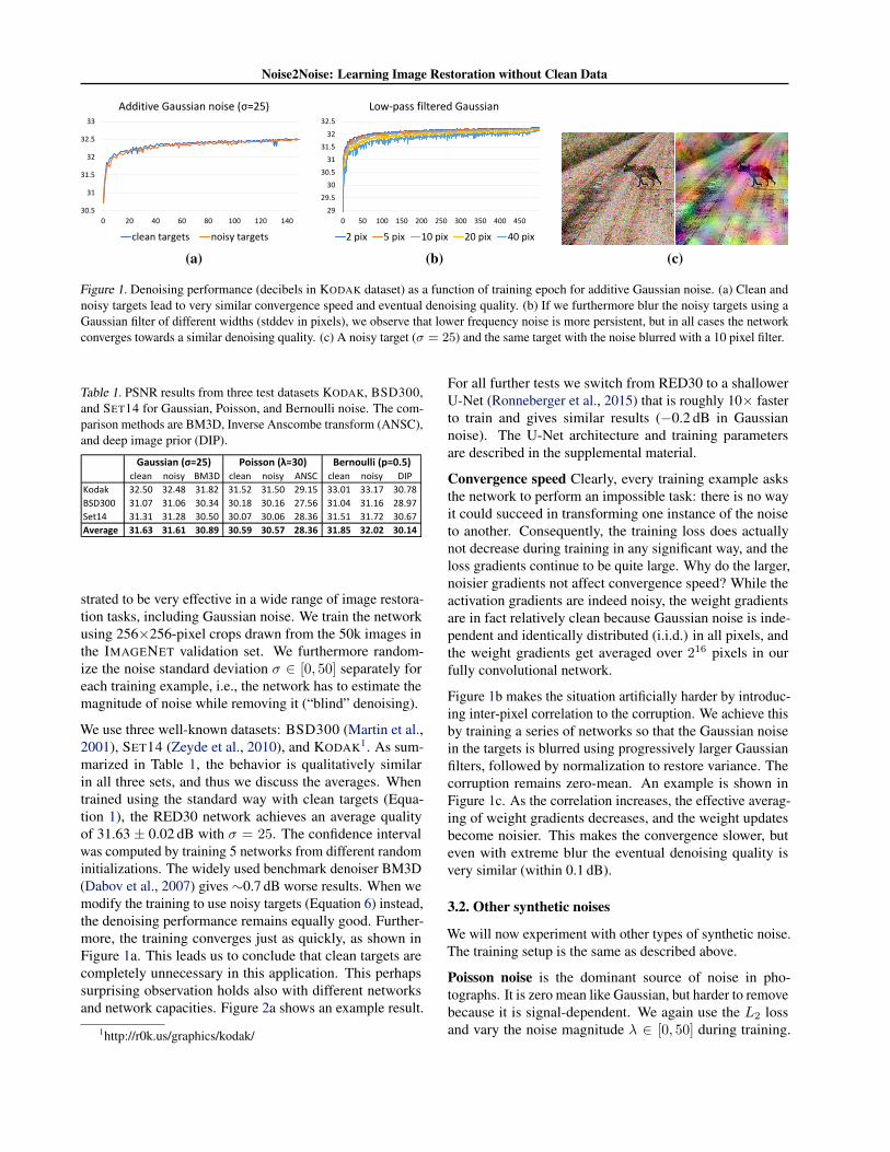
Figure 1. Denoising performance (decibels in KODAK dataset) as a function of training epoch for additive Gaussian noise. (a) Clean andnoisy targets lead to very similar convergence speed and eventual denoising quality. (b) If we furthermore blur the noisy targets using aGaussian filter of different widths (stddev in pixels), we observe that lower frequency noise is more persistent, but in all cases the networkconverges towards a similar denoising quality. (c) A noisy target (σ = 25) and the same target with the noise blurred with a 10 pixel filter.

Table 1. PSNR results from three test datasets KODAK, BSD300,and SET14 for Gaussian, Poisson, and Bernoulli noise. The com-parison methods are BM3D, Inverse Anscombe transform (ANSC),and deep image prior (DIP).

clean noisy BM3D clean noisy ANSC clean noisy DIP

Kodak 32.50 32.48 31.82 31.52 31.50 29.15 33.01 33.17 30.78

BSD300 31.07 31.06 30.34 30.18 30.16 27.56 31.04 31.16 28.97

Set14 31.31 31.28 30.50 30.07 30.06 28.36 31.51 31.72 30.67

Average 31.63 31.61 30.89 30.59 30.57 28.36 31.85 32.02 30.14

Bernoulli (p=0.5)Gaussian (σ=25) Poisson (λ=30)

strated to be very effective in a wide range of image restora-tion tasks, including Gaussian noise. We train the networkusing 256×256-pixel crops drawn from the 50k images inthe IMAGENET validation set. We furthermore random-ize the noise standard deviation σ ∈ [0, 50] separately foreach training example, i.e., the network has to estimate themagnitude of noise while removing it (“blind” denoising).

We use three well-known datasets: BSD300 (Martin et al.,2001), SET14 (Zeyde et al., 2010), and KODAK1. As sum-marized in Table 1, the behavior is qualitatively similarin all three sets, and thus we discuss the averages. Whentrained using the standard way with clean targets (Equa-tion 1), the RED30 network achieves an average qualityof 31.63 ± 0.02 dB with σ = 25. The confidence intervalwas computed by training 5 networks from different randominitializations. The widely used benchmark denoiser BM3D(Dabov et al., 2007) gives ∼0.7 dB worse results. When wemodify the training to use noisy targets (Equation 6) instead,the denoising performance remains equally good. Further-more, the training converges just as quickly, as shown inFigure 1a. This leads us to conclude that clean targets arecompletely unnecessary in this application. This perhapssurprising observation holds also with different networksand network capacities. Figure 2a shows an example result.

1http://r0k.us/graphics/kodak/

For all further tests we switch from RED30 to a shallowerU-Net (Ronneberger et al., 2015) that is roughly 10× fasterto train and gives similar results (−0.2 dB in Gaussiannoise). The U-Net architecture and training parametersare described in the supplemental material.

Convergence speed Clearly, every training example asksthe network to perform an impossible task: there is no wayit could succeed in transforming one instance of the noiseto another. Consequently, the training loss does actuallynot decrease during training in any significant way, and theloss gradients continue to be quite large. Why do the larger,noisier gradients not affect convergence speed? While theactivation gradients are indeed noisy, the weight gradientsare in fact relatively clean because Gaussian noise is inde-pendent and identically distributed (i.i.d.) in all pixels, andthe weight gradients get averaged over 216 pixels in ourfully convolutional network.

Figure 1b makes the situation artificially harder by introduc-ing inter-pixel correlation to the corruption. We achieve thisby training a series of networks so that the Gaussian noisein the targets is blurred using progressively larger Gaussianfilters, followed by normalization to restore variance. Thecorruption remains zero-mean. An example is shown inFigure 1c. As the correlation increases, the effective averag-ing of weight gradients decreases, and the weight updatesbecome noisier. This makes the convergence slower, buteven with extreme blur the eventual denoising quality isvery similar (within 0.1 dB).

3.2. Other synthetic noises

We will now experiment with other types of synthetic noise.The training setup is the same as described above.

Poisson noise is the dominant source of noise in pho-tographs. It is zero mean like Gaussian, but harder to removebecause it is signal-dependent. We again use the L2 lossand vary the noise magnitude λ ∈ [0, 50] during training.


When clean target images are used, we get an average of30.59± 0.02 dB, while noisy targets give an equally good30.57 ± 0.02 dB, again at similar convergence speed. Acomparison method based on Ascombe transform (Makitalo& Foi, 2011) — which first transforms the input so thatPoisson noise turns into Gaussian noise, removes it usingBM3D, and finally does an inverse transform — gives over2 dB lower quality than our method.

The other forms of noise in cameras, e.g. dark current andquantization, are small compared to Poisson noise, can bemade zero-mean (Hasinoff et al., 2016), and hence pose noproblems for training with noisy targets. We conclude thatnoise-free training data is unnecessary in this application.

That said, saturation (gamut clipping) does break our as-sumptions, as parts of the noise distribution are discardedand the expectation of the remaining part is no longer cor-rect. Saturation is unwanted for other reasons as well, sothis is not a significant practical limitation.

Multiplicative Bernoulli noise (aka binomial noise) con-structs a random mask m that is 1 for valid pixels and 0 forzeroed/missing pixels. To avoid backpropagating gradientsfrom missing pixels, we exclude them from the loss usingthat mask:

argminθ

∑i

(m� (fθ(xi)− yi))2, (7)

as described by Ulyanov et al. (2017) in the context of theirdeep image prior (DIP).

The probability of corrupted pixels is denoted with p; in ourtraining we vary p ∈ [0.0, 0.95] and during testing p = 0.5.Training with clean targets gives an average of 31.85 ±0.03 dB, noisy targets (separate m for input and target) givea slightly higher 32.02 ± 0.03 dB, possibly because noisytargets effectively implement a form of dropout (Srivastavaet al., 2014) at the network output. DIP was almost 2 dBworse – DIP is not a learning-based solution, and as suchvery different from our approach, but it shares the propertythat neither clean examples nor an explicit model of thecorruption is needed. We used the “Image reconstruction”setup as described in the DIP supplemental material.2

Text removal Figure 3 demonstrates blind text removal.The corruption consists of a large, varying number of ran-dom strings in random places, also on top of each other, andfurthermore so that the font size and color are randomizedas well. The font and string orientation remain fixed.

The network is trained using independently corrupted inputand target pairs. The probability of corrupted pixels p isapproximately [0, 0.5] during training, and p ≈ 0.25 duringtesting. In this test the mean (L2 loss) is not the correctanswer because the overlaid text has colors unrelated to the

2https://dmitryulyanov.github.io/deep image prior

(a) Gaussian (σ = 25)

BM

3D

(b) Poisson (λ = 30)

AN

SC

OM

BE

(c) Bernoulli (p = 0.5)

DE

EP

IMA

GE

PR

IOR

Ground truth Input Our Comparison

Figure 2. Example results for Gaussian, Poisson, and Bernoullinoise. Our result was computed by using noisy targets — thecorresponding result with clean targets is omitted because it isvirtually identical in all three cases, as discussed in the text. Adifferent comparison method is used for each noise type.

actual image, and the resulting image would incorrectly tendtowards a linear combination of the right answer and theaverage text color (medium gray). However, with any rea-sonable amount of overlaid text, a pixel retains the originalcolor more often than not, and therefore the median is thecorrect statistic. Hence, we use L1 = |fθ(x)− y| as the lossfunction. Figure 3 shows an example result.

Random-valued impulse noise replaces some pixels withnoise and retains the colors of others. Instead of the standardsalt and pepper noise (randomly replacing pixels with blackor white), we study a harder distribution where each pixelis replaced with a random color drawn from the uniformdistribution [0, 1]3 with probability p and retains its colorwith probability 1− p. The pixels’ color distributions are aDirac at the original color plus a uniform distribution, withrelative weights given by the replacement probability p. Inthis case, neither the mean nor the median yield the correctresult; the desired output is the mode of the distribution(the Dirac spike). The distribution remains unimodal. Forapproximate mode seeking, we use an annealed version


p ≈ 0.04 p ≈ 0.42

Example training pairs Input (p ≈ 0.25) L2 L1 Clean targets Ground truth17.12 dB 26.89 dB 35.75 dB 35.82 dB PSNR

Figure 3. In case of text removal the mean (L2 loss) is not the correct answer but median (L1) is.

p = 0.22 p = 0.81

Example training pairs Input (p = 0.70) L2 / L1 L0 Clean targets Ground truth8.89 dB 13.02 dB / 16.36 dB 28.43 dB 28.86 dB PSNR

Figure 4. In case of random-valued impulse noise the mode (L0) produces unbiased results, unlike mean (L2) or median (L1).

-10

-5

0

10% 20% 30% 40% 50% 60% 70% 80% 90%

PSNR delta from clean targets

L0 L1

Figure 5. PSNR of noisy-target training relative to clean targetswith a varying percentage of target pixels corrupted by RGB im-pulse noise. In this test a separate network was trained for each cor-ruption level, and the graph was averaged over the KODAK dataset.

of the “L0 loss” function defined as (|fθ(x) − y| + ε)γ ,where ε = 10−8, where γ is annealed linearly from 2 to 0during training. This annealing did not cause any numericalissues in our tests. The relationship of the L0 loss and modeseeking is analyzed in the supplement.

We again train the network using noisy inputs and noisytargets, where the probability of corrupted pixels is random-ized separately for each pair from [0, 0.95]. Figure 4 showsthe inference results when 70% input pixels are randomized.Training with L2 loss biases the results heavily towards gray,because the result tends towards a linear combination thecorrect answer and and mean of the uniform random corrup-

tion. As predicted by theory, the L1 loss gives good resultsas long as fewer than 50% of the pixels are randomized,but beyond that threshold it quickly starts to bias dark andbright areas towards gray (Figure 5). L0, on the other hand,shows little bias even with extreme corruptions (e.g. 90%pixels), because of all the possible pixel values, the correctanswer (e.g. 10%) is still the most common.

3.3. Monte Carlo rendering

Physically accurate renderings of virtual environments aremost often generated through a process known as MonteCarlo path tracing. This amounts to drawing random se-quences of scattering events (“light paths”) in the scene thatconnect light sources and virtual sensors, and integratingthe radiance carried by them over all possible paths (Veach& Guibas, 1995). The Monte Carlo integrator is constructedsuch that the intensity of each pixel is the expectation ofthe random path sampling process, i.e., the sampling noiseis zero-mean. However, despite decades of research intoimportance sampling techniques, little else can be said aboutthe distribution. It varies from pixel to pixel, heavily de-pends on the scene configuration and rendering parameters,and can be arbitrarily multimodal. Some lighting effects,


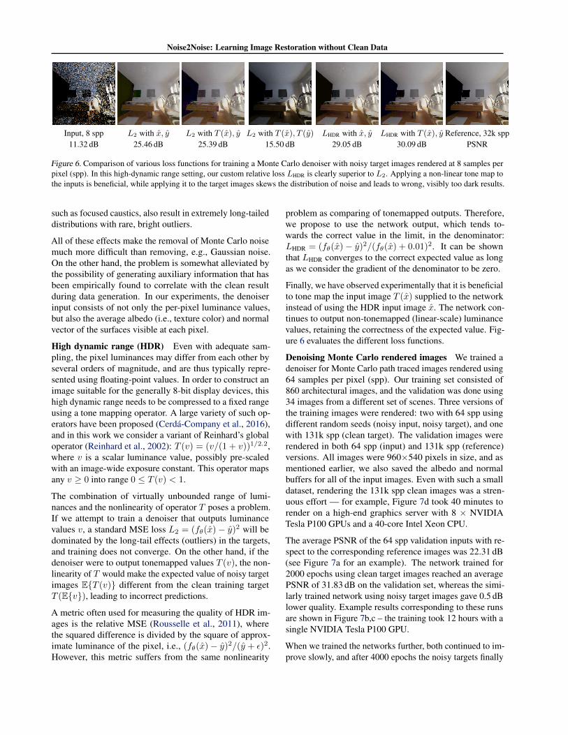
Input, 8 spp L2 with x, y L2 with T (x), y L2 with T (x), T (y) LHDR with x, y LHDR with T (x), y Reference, 32k spp11.32 dB 25.46 dB 25.39 dB 15.50 dB 29.05 dB 30.09 dB PSNR

Figure 6. Comparison of various loss functions for training a Monte Carlo denoiser with noisy target images rendered at 8 samples perpixel (spp). In this high-dynamic range setting, our custom relative loss LHDR is clearly superior to L2. Applying a non-linear tone map tothe inputs is beneficial, while applying it to the target images skews the distribution of noise and leads to wrong, visibly too dark results.

such as focused caustics, also result in extremely long-taileddistributions with rare, bright outliers.

All of these effects make the removal of Monte Carlo noisemuch more difficult than removing, e.g., Gaussian noise.On the other hand, the problem is somewhat alleviated bythe possibility of generating auxiliary information that hasbeen empirically found to correlate with the clean resultduring data generation. In our experiments, the denoiserinput consists of not only the per-pixel luminance values,but also the average albedo (i.e., texture color) and normalvector of the surfaces visible at each pixel.

High dynamic range (HDR) Even with adequate sam-pling, the pixel luminances may differ from each other byseveral orders of magnitude, and are thus typically repre-sented using floating-point values. In order to construct animage suitable for the generally 8-bit display devices, thishigh dynamic range needs to be compressed to a fixed rangeusing a tone mapping operator. A large variety of such op-erators have been proposed (Cerda-Company et al., 2016),and in this work we consider a variant of Reinhard’s globaloperator (Reinhard et al., 2002): T (v) = (v/(1 + v))1/2.2,where v is a scalar luminance value, possibly pre-scaledwith an image-wide exposure constant. This operator mapsany v ≥ 0 into range 0 ≤ T (v) < 1.

The combination of virtually unbounded range of lumi-nances and the nonlinearity of operator T poses a problem.If we attempt to train a denoiser that outputs luminancevalues v, a standard MSE loss L2 = (fθ(x)− y)2 will bedominated by the long-tail effects (outliers) in the targets,and training does not converge. On the other hand, if thedenoiser were to output tonemapped values T (v), the non-linearity of T would make the expected value of noisy targetimages E{T (v)} different from the clean training targetT (E{v}), leading to incorrect predictions.

A metric often used for measuring the quality of HDR im-ages is the relative MSE (Rousselle et al., 2011), wherethe squared difference is divided by the square of approx-imate luminance of the pixel, i.e., (fθ(x)− y)2/(y + ε)2.However, this metric suffers from the same nonlinearity

problem as comparing of tonemapped outputs. Therefore,we propose to use the network output, which tends to-wards the correct value in the limit, in the denominator:LHDR = (fθ(x)− y)2/(fθ(x) + 0.01)2. It can be shownthat LHDR converges to the correct expected value as longas we consider the gradient of the denominator to be zero.

Finally, we have observed experimentally that it is beneficialto tone map the input image T (x) supplied to the networkinstead of using the HDR input image x. The network con-tinues to output non-tonemapped (linear-scale) luminancevalues, retaining the correctness of the expected value. Fig-ure 6 evaluates the different loss functions.

Denoising Monte Carlo rendered images We trained adenoiser for Monte Carlo path traced images rendered using64 samples per pixel (spp). Our training set consisted of860 architectural images, and the validation was done using34 images from a different set of scenes. Three versions ofthe training images were rendered: two with 64 spp usingdifferent random seeds (noisy input, noisy target), and onewith 131k spp (clean target). The validation images wererendered in both 64 spp (input) and 131k spp (reference)versions. All images were 960×540 pixels in size, and asmentioned earlier, we also saved the albedo and normalbuffers for all of the input images. Even with such a smalldataset, rendering the 131k spp clean images was a stren-uous effort — for example, Figure 7d took 40 minutes torender on a high-end graphics server with 8 × NVIDIATesla P100 GPUs and a 40-core Intel Xeon CPU.

The average PSNR of the 64 spp validation inputs with re-spect to the corresponding reference images was 22.31 dB(see Figure 7a for an example). The network trained for2000 epochs using clean target images reached an averagePSNR of 31.83 dB on the validation set, whereas the simi-larly trained network using noisy target images gave 0.5 dBlower quality. Example results corresponding to these runsare shown in Figure 7b,c – the training took 12 hours with asingle NVIDIA Tesla P100 GPU.

When we trained the networks further, both continued to im-prove slowly, and after 4000 epochs the noisy targets finally


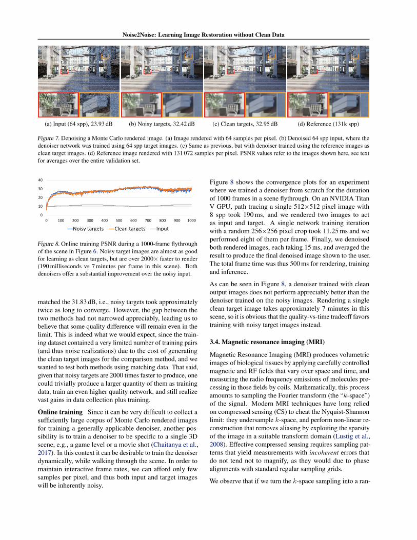
(a) Input (64 spp), 23.93 dB (b) Noisy targets, 32.42 dB (c) Clean targets, 32.95 dB (d) Reference (131k spp)

Figure 7. Denoising a Monte Carlo rendered image. (a) Image rendered with 64 samples per pixel. (b) Denoised 64 spp input, where thedenoiser network was trained using 64 spp target images. (c) Same as previous, but with denoiser trained using the reference images asclean target images. (d) Reference image rendered with 131 072 samples per pixel. PSNR values refer to the images shown here, see textfor averages over the entire validation set.

0

10

20

30

40

0 100 200 300 400 500 600 700 800 900 1000

PSNR

Noisy targets Clean targets Input

Figure 8. Online training PSNR during a 1000-frame flythroughof the scene in Figure 6. Noisy target images are almost as goodfor learning as clean targets, but are over 2000× faster to render(190 milliseconds vs 7 minutes per frame in this scene). Bothdenoisers offer a substantial improvement over the noisy input.

matched the 31.83 dB, i.e., noisy targets took approximatelytwice as long to converge. However, the gap between thetwo methods had not narrowed appreciably, leading us tobelieve that some quality difference will remain even in thelimit. This is indeed what we would expect, since the train-ing dataset contained a very limited number of training pairs(and thus noise realizations) due to the cost of generatingthe clean target images for the comparison method, and wewanted to test both methods using matching data. That said,given that noisy targets are 2000 times faster to produce, onecould trivially produce a larger quantity of them as trainingdata, train an even higher quality network, and still realizevast gains in data collection plus training.

Online training Since it can be very difficult to collect asufficiently large corpus of Monte Carlo rendered imagesfor training a generally applicable denoiser, another pos-sibility is to train a denoiser to be specific to a single 3Dscene, e.g., a game level or a movie shot (Chaitanya et al.,2017). In this context it can be desirable to train the denoiserdynamically, while walking through the scene. In order tomaintain interactive frame rates, we can afford only fewsamples per pixel, and thus both input and target imageswill be inherently noisy.

Figure 8 shows the convergence plots for an experimentwhere we trained a denoiser from scratch for the durationof 1000 frames in a scene flythrough. On an NVIDIA TitanV GPU, path tracing a single 512×512 pixel image with8 spp took 190 ms, and we rendered two images to actas input and target. A single network training iterationwith a random 256×256 pixel crop took 11.25 ms and weperformed eight of them per frame. Finally, we denoisedboth rendered images, each taking 15 ms, and averaged theresult to produce the final denoised image shown to the user.The total frame time was thus 500 ms for rendering, trainingand inference.

As can be seen in Figure 8, a denoiser trained with cleanoutput images does not perform appreciably better than thedenoiser trained on the noisy images. Rendering a singleclean target image takes approximately 7 minutes in thisscene, so it is obvious that the quality-vs-time tradeoff favorstraining with noisy target images instead.

3.4. Magnetic resonance imaging (MRI)

Magnetic Resonance Imaging (MRI) produces volumetricimages of biological tissues by applying carefully controlledmagnetic and RF fields that vary over space and time, andmeasuring the radio frequency emissions of molecules pre-cessing in those fields by coils. Mathematically, this processamounts to sampling the Fourier transform (the “k-space”)of the signal. Modern MRI techniques have long reliedon compressed sensing (CS) to cheat the Nyquist-Shannonlimit: they undersample k-space, and perform non-linear re-construction that removes aliasing by exploiting the sparsityof the image in a suitable transform domain (Lustig et al.,2008). Effective compressed sensing requires sampling pat-terns that yield measurements with incoherent errors thatdo not tend not to magnify, as they would due to phasealignments with standard regular sampling grids.

We observe that if we turn the k-space sampling into a ran-


dom process with a known probability density p(k) over thefrequencies k, our main idea applies. In particular, we modelthe k-space sampling operation as a Bernoulli process whereeach individual frequency has a probability p(k) = e−λ|k|

of being selected for acquisition.3 The frequencies that areretained are weighted by the inverse of the selection proba-bility, and non-chosen frequencies are set to zero. Clearly,the expectation of this “Russian roulette” process is thecorrect spectrum. The parameter λ controls the overall frac-tion of k-space retained; in the following experiments, wechoose it so that 10% of the samples are retained relative to afull Nyquist-Shannon sampling. The undersampled spectraare transformed to the primal image domain by the standardinverse Fourier transform. An example of an undersam-pled input/target picture, the corresponding fully sampledreference, and their spectra, are shown in Figure 9(a, d).

Now we simply set up a regression problem of the form (6)and train a convolutional neural network using pairs of twoindependent undersampled images x and y of the same vol-ume. As the spectra of the input and target are correct on ex-pectation, and the Fourier transform is linear, we use the L2

loss. Additionally, we improve the result slightly by enforc-ing the exact preservation of frequencies that are present inthe input image x by Fourier transforming the result fθ(x),replacing the frequencies with those from the input, andtransforming back to the primal domain before computingthe loss: the final loss reads (F−1(Rx(F(fθ(x)))) − y)2,where R denotes the replacement of non-zero frequenciesfrom the input. This process is trained end-to-end.

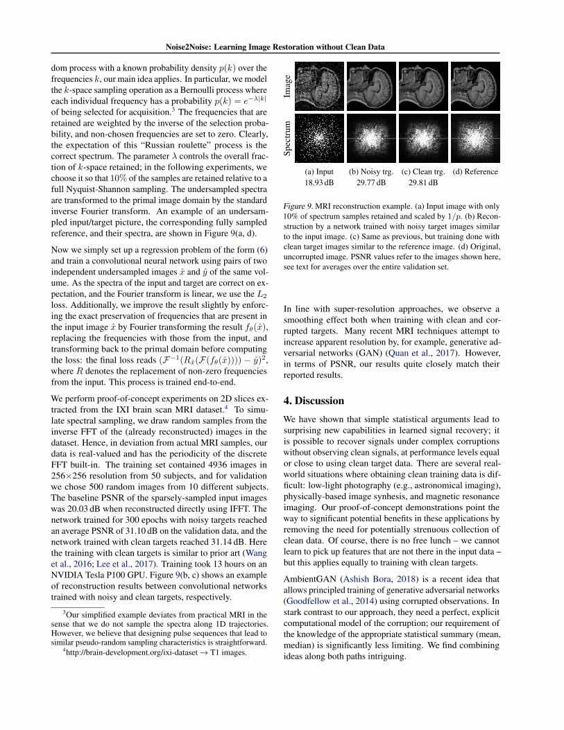
We perform proof-of-concept experiments on 2D slices ex-tracted from the IXI brain scan MRI dataset.4 To simu-late spectral sampling, we draw random samples from theinverse FFT of the (already reconstructed) images in thedataset. Hence, in deviation from actual MRI samples, ourdata is real-valued and has the periodicity of the discreteFFT built-in. The training set contained 4936 images in256×256 resolution from 50 subjects, and for validationwe chose 500 random images from 10 different subjects.The baseline PSNR of the sparsely-sampled input imageswas 20.03 dB when reconstructed directly using IFFT. Thenetwork trained for 300 epochs with noisy targets reachedan average PSNR of 31.10 dB on the validation data, and thenetwork trained with clean targets reached 31.14 dB. Herethe training with clean targets is similar to prior art (Wanget al., 2016; Lee et al., 2017). Training took 13 hours on anNVIDIA Tesla P100 GPU. Figure 9(b, c) shows an exampleof reconstruction results between convolutional networkstrained with noisy and clean targets, respectively.

3Our simplified example deviates from practical MRI in thesense that we do not sample the spectra along 1D trajectories.However, we believe that designing pulse sequences that lead tosimilar pseudo-random sampling characteristics is straightforward.

4http://brain-development.org/ixi-dataset→ T1 images.

Imag

eSp

ectr

um

(a) Input (b) Noisy trg. (c) Clean trg. (d) Reference18.93 dB 29.77 dB 29.81 dB

Figure 9. MRI reconstruction example. (a) Input image with only10% of spectrum samples retained and scaled by 1/p. (b) Recon-struction by a network trained with noisy target images similarto the input image. (c) Same as previous, but training done withclean target images similar to the reference image. (d) Original,uncorrupted image. PSNR values refer to the images shown here,see text for averages over the entire validation set.

In line with super-resolution approaches, we observe asmoothing effect both when training with clean and cor-rupted targets. Many recent MRI techniques attempt toincrease apparent resolution by, for example, generative ad-versarial networks (GAN) (Quan et al., 2017). However,in terms of PSNR, our results quite closely match theirreported results.

4. DiscussionWe have shown that simple statistical arguments lead tosurprising new capabilities in learned signal recovery; itis possible to recover signals under complex corruptionswithout observing clean signals, at performance levels equalor close to using clean target data. There are several real-world situations where obtaining clean training data is dif-ficult: low-light photography (e.g., astronomical imaging),physically-based image synhesis, and magnetic resonanceimaging. Our proof-of-concept demonstrations point theway to significant potential benefits in these applications byremoving the need for potentially strenuous collection ofclean data. Of course, there is no free lunch – we cannotlearn to pick up features that are not there in the input data –but this applies equally to training with clean targets.

AmbientGAN (Ashish Bora, 2018) is a recent idea thatallows principled training of generative adversarial networks(Goodfellow et al., 2014) using corrupted observations. Instark contrast to our approach, they need a perfect, explicitcomputational model of the corruption; our requirement ofthe knowledge of the appropriate statistical summary (mean,median) is significantly less limiting. We find combiningideas along both paths intriguing.


AcknowledgmentsBill Dally, David Luebke, Aaron Lefohn for discussions andsupporting the research; NVIDIA Research staff for sugges-tions and discussion; Runa Lober and Gunter Sprenger forsynthetic off-line training data; Jacopo Pantaleoni for theinteractive renderer used in on-line training; Samuli Vuori-nen for initial photography test data; Koos Zevenhoven fordiscussions on MRI basics.

ReferencesAshish Bora, Eric Price, Alexandros G. Dimakis. Ambi-

entGAN: Generative models from lossy measurements.ICLR, 2018.

Cerda-Company, Xim, Parraga, C. Alejandro, and Otazu,Xavier. Which tone-mapping operator is the best?A comparative study of perceptual quality. CoRR,abs/1601.04450, 2016.

Chaitanya, Chakravarty R. Alla, Kaplanyan, Anton S.,Schied, Christoph, Salvi, Marco, Lefohn, Aaron,Nowrouzezahrai, Derek, and Aila, Timo. Interactivereconstruction of Monte Carlo image sequences using arecurrent denoising autoencoder. ACM Trans. Graph., 36(4):98:1–98:12, 2017.

Dabov, K., Foi, A., Katkovnik, V., and Egiazarian, K. Imagedenoising by sparse 3-D transform-domain collaborativefiltering. IEEE Trans. Image Process., 16(8):2080–2095,2007.

Goodfellow, Ian, Pouget-Abadie, Jean, Mirza, Mehdi, Xu,Bing, Warde-Farley, David, Ozair, Sherjil, Courville,Aaron, and Bengio, Yoshua. Generative Adversarial Net-works. In NIPS, 2014.

Hasinoff, Sam, Sharlet, Dillon, Geiss, Ryan, Adams, An-drew, Barron, Jonathan T., Kainz, Florian, Chen, Jiawen,and Levoy, Marc. Burst photography for high dynamicrange and low-light imaging on mobile cameras. ACMTrans. Graph., 35(6):192:1–192:12, 2016.

He, Kaiming, Zhang, Xiangyu, Ren, Shaoqing, and Sun,Jian. Delving deep into rectifiers: Surpassing human-level performance on imagenet classification. CoRR,abs/1502.01852, 2015.

Huber, Peter J. Robust estimation of a location parameter.Ann. Math. Statist., 35(1):73–101, 1964.

Iizuka, Satoshi, Simo-Serra, Edgar, and Ishikawa, Hiroshi.Globally and locally consistent image completion. ACMTrans. Graph., 36(4):107:1–107:14, 2017.

Isola, Phillip, Zhu, Jun-Yan, Zhou, Tinghui, and Efros,Alexei A. Image-to-image translation with conditionaladversarial networks. In Proc. CVPR 2017, 2017.

Kingma, Diederik P. and Ba, Jimmy. Adam: A method forstochastic optimization. In ICLR, 2015.

Ledig, Christian, Theis, Lucas, Huszar, Ferenc, Caballero,Jose, Aitken, Andrew P., Tejani, Alykhan, Totz, Johannes,Wang, Zehan, and Shi, Wenzhe. Photo-realistic singleimage super-resolution using a generative adversarial net-work. In Proc. CVPR, pp. 105–114, 2017.

Lee, D., Yoo, J., and Ye, J. C. Deep residual learning forcompressed sensing MRI. In Proc. IEEE 14th Interna-tional Symposium on Biomedical Imaging (ISBI 2017),pp. 15–18, 2017.

Lustig, Michael, Donoho, David L., Santos, Juan M., andPauly, John M. Compressed sensing MRI. In IEEE SignalProcessing Magazine, volume 25, pp. 72–82, 2008.

Maas, Andrew L, Hannun, Awni Y, and Ng, Andrew. Recti-fier nonlinearities improve neural network acoustic mod-els. In Proc. International Conference on Machine Learn-ing (ICML), volume 30, 2013.

Mao, Xiao-Jiao, Shen, Chunhua, and Yang, Yu-Bin. Im-age restoration using convolutional auto-encoders withsymmetric skip connections. In Proc. NIPS, 2016.

Martin, D., Fowlkes, C., Tal, D., and Malik, J. A databaseof human segmented natural images and its applicationto evaluating segmentation algorithms and measuringecological statistics. In Proc. ICCV, volume 2, pp. 416–423, 2001.

Makitalo, Markku and Foi, Alessandro. Optimal inversionof the Anscombe transformation in low-count Poissonimage denoising. IEEE Trans. Image Process., 20(1):99–109, 2011.

Quan, Tran Minh, Nguyen-Duc, Thanh, and Jeong, Won-Ki. Compressed sensing MRI reconstruction withcyclic loss in generative adversarial networks. CoRR,abs/1709.00753, 2017.

Reinhard, Erik, Stark, Michael, Shirley, Peter, and Ferwerda,James. Photographic tone reproduction for digital images.ACM Trans. Graph., 21(3):267–276, 2002.

Ronneberger, Olaf, Fischer, Philipp, and Brox, Thomas.U-net: Convolutional networks for biomedical imagesegmentation. MICCAI, 9351:234–241, 2015.

Rousselle, Fabrice, Knaus, Claude, and Zwicker, Matthias.Adaptive sampling and reconstruction using greedy errorminimization. ACM Trans. Graph., 30(6):159:1–159:12,2011.

Srivastava, Nitish, Hinton, Geoffrey, Krizhevsky, Alex,Sutskever, Ilya, and Salakhutdinov, Ruslan. Dropout:


A simple way to prevent neural networks from overfitting.Journal of Machine Learning Research, 15:1929–1958,2014.

Ulyanov, Dmitry, Vedaldi, Andrea, and Lempitsky, Victor S.Deep image prior. CoRR, abs/1711.10925, 2017.

Veach, Eric and Guibas, Leonidas J. Optimally combiningsampling techniques for Monte Carlo rendering. In Proc.ACM SIGGRAPH 95, pp. 419–428, 1995.

Wang, S., Su, Z., Ying, L., Peng, X., Zhu, S., Liang, F.,Feng, D., and Liang, D. Accelerating magnetic resonanceimaging via deep learning. In Proc. IEEE 13th Inter-national Symposium on Biomedical Imaging (ISBI), pp.514–517, 2016.

Zeyde, R., Elad, M., and Protter, M. On single image scale-up using sparse-representations. In Proc. Curves andSurfaces: 7th International Conference, pp. 711–730,2010.

Zhang, Richard, Isola, Phillip, and Efros, Alexei A. Colorfulimage colorization. In Proc. ECCV, pp. 649–666, 2016.


A. AppendixA.1. Network architecture

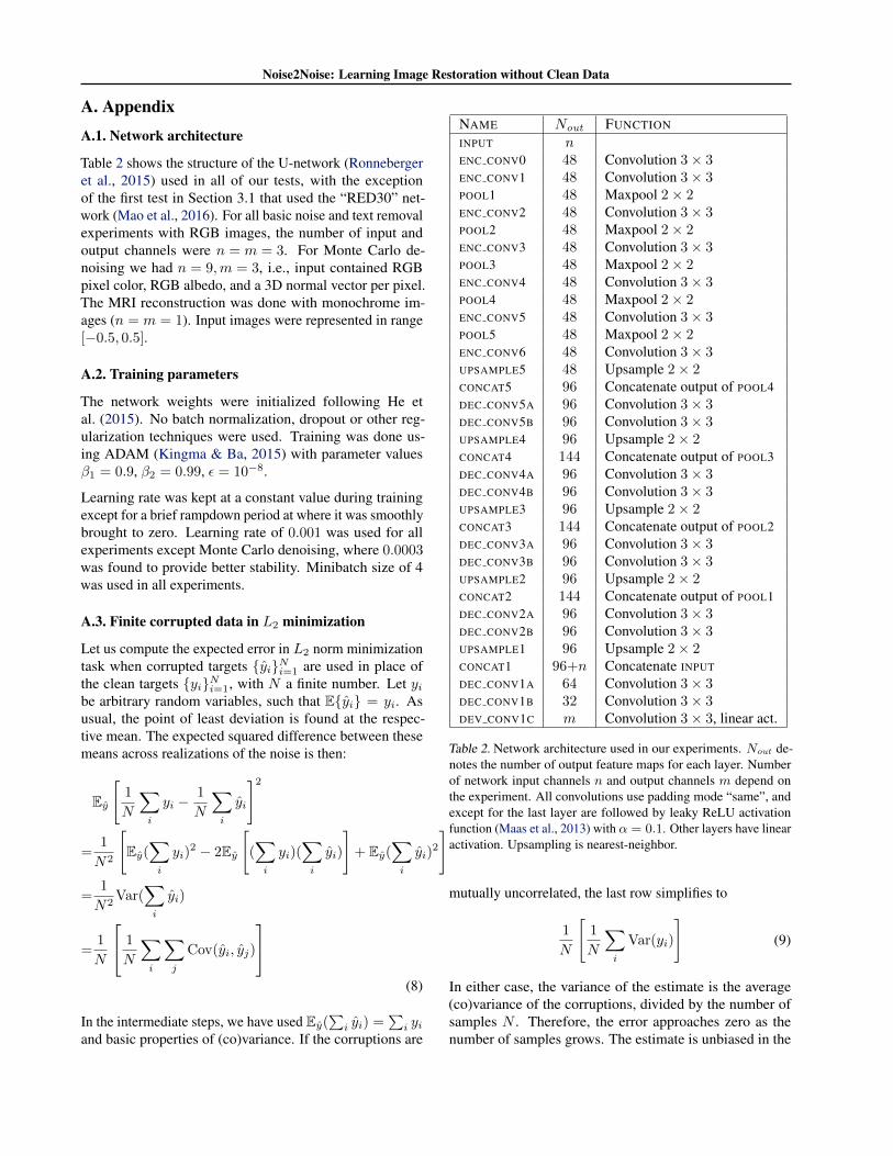
Table 2 shows the structure of the U-network (Ronnebergeret al., 2015) used in all of our tests, with the exceptionof the first test in Section 3.1 that used the “RED30” net-work (Mao et al., 2016). For all basic noise and text removalexperiments with RGB images, the number of input andoutput channels were n = m = 3. For Monte Carlo de-noising we had n = 9,m = 3, i.e., input contained RGBpixel color, RGB albedo, and a 3D normal vector per pixel.The MRI reconstruction was done with monochrome im-ages (n = m = 1). Input images were represented in range[−0.5, 0.5].

A.2. Training parameters

The network weights were initialized following He etal. (2015). No batch normalization, dropout or other reg-ularization techniques were used. Training was done us-ing ADAM (Kingma & Ba, 2015) with parameter valuesβ1 = 0.9, β2 = 0.99, ε = 10−8.

Learning rate was kept at a constant value during trainingexcept for a brief rampdown period at where it was smoothlybrought to zero. Learning rate of 0.001 was used for allexperiments except Monte Carlo denoising, where 0.0003was found to provide better stability. Minibatch size of 4was used in all experiments.

A.3. Finite corrupted data in L2 minimization

Let us compute the expected error in L2 norm minimizationtask when corrupted targets {yi}Ni=1 are used in place ofthe clean targets {yi}Ni=1, with N a finite number. Let yibe arbitrary random variables, such that E{yi} = yi. Asusual, the point of least deviation is found at the respec-tive mean. The expected squared difference between thesemeans across realizations of the noise is then:

Ey

[1

N

∑i

yi −1

N

∑i

yi

]2

=1

N2

[Ey(

∑i

yi)2 − 2Ey

[(∑i

yi)(∑i

yi)

]+ Ey(

∑i

yi)2

]

=1

N2Var(

∑i

yi)

=1

N

1

N

∑i

∑j

Cov(yi, yj)

(8)

In the intermediate steps, we have used Ey(∑i yi) =

∑i yi

and basic properties of (co)variance. If the corruptions are

NAME Nout FUNCTION

INPUT nENC CONV0 48 Convolution 3× 3ENC CONV1 48 Convolution 3× 3POOL1 48 Maxpool 2× 2ENC CONV2 48 Convolution 3× 3POOL2 48 Maxpool 2× 2ENC CONV3 48 Convolution 3× 3POOL3 48 Maxpool 2× 2ENC CONV4 48 Convolution 3× 3POOL4 48 Maxpool 2× 2ENC CONV5 48 Convolution 3× 3POOL5 48 Maxpool 2× 2ENC CONV6 48 Convolution 3× 3UPSAMPLE5 48 Upsample 2× 2CONCAT5 96 Concatenate output of POOL4DEC CONV5A 96 Convolution 3× 3DEC CONV5B 96 Convolution 3× 3UPSAMPLE4 96 Upsample 2× 2CONCAT4 144 Concatenate output of POOL3DEC CONV4A 96 Convolution 3× 3DEC CONV4B 96 Convolution 3× 3UPSAMPLE3 96 Upsample 2× 2CONCAT3 144 Concatenate output of POOL2DEC CONV3A 96 Convolution 3× 3DEC CONV3B 96 Convolution 3× 3UPSAMPLE2 96 Upsample 2× 2CONCAT2 144 Concatenate output of POOL1DEC CONV2A 96 Convolution 3× 3DEC CONV2B 96 Convolution 3× 3UPSAMPLE1 96 Upsample 2× 2CONCAT1 96+n Concatenate INPUT

DEC CONV1A 64 Convolution 3× 3DEC CONV1B 32 Convolution 3× 3DEV CONV1C m Convolution 3× 3, linear act.

Table 2. Network architecture used in our experiments. Nout de-notes the number of output feature maps for each layer. Numberof network input channels n and output channels m depend onthe experiment. All convolutions use padding mode “same”, andexcept for the last layer are followed by leaky ReLU activationfunction (Maas et al., 2013) with α = 0.1. Other layers have linearactivation. Upsampling is nearest-neighbor.

mutually uncorrelated, the last row simplifies to

1

N

[1

N

∑i

Var(yi)

](9)

In either case, the variance of the estimate is the average(co)variance of the corruptions, divided by the number ofsamples N . Therefore, the error approaches zero as thenumber of samples grows. The estimate is unbiased in the


sense that it is correct on expectation, even with a finiteamount of data.

The above derivation assumes scalar target variables. Whenyi are images, N is to be taken as the total number of scalarsin the images, i.e., #images × #pixels/image × #color chan-nels.

A.4. Mode seeking and the “L0” norm

Interestingly, while the “L0 norm” could intuitively be ex-pected to converge to an exact mode, i.e. a local maximumof the probability density function of the data, theoreticalanalysis reveals that it recovers a slightly different point.While an actual mode is a zero-crossing of the derivative ofthe PDF, the L0 norm minimization recovers a zero-crossingof its Hilbert transform instead. We have verified this behav-ior in a variety of numerical experiments, and, in practice,we find that the estimate is typically close to the true mode.This can be explained by the fact that the Hilbert transformapproximates differentiation (with a sign flip): the latter isa multiplication by iω in the Fourier domain, whereas theHilbert transform is a multiplication by −i sgn(ω).

For a continuous data density q(x), the norm minimizationtask for Lp amounts to finding a point x∗ that has a min-imal expected p-norm distance (suitably normalized, andomitting the pth root) from points y ∼ q(y):

x∗ = argminx

Ey∼q{1

p|x− y|p}

= argminx

∫1

p|x− y|pq(y) dy

(10)

Following the typical procedure, the minimizer is found at aroot of the derivative of the expression under argmin:

0 =∂

∂x

∫1

p|x− y|pq(y) dy

=

∫sgn(x− y)|x− y|p−1q(y) dy

(11)

This equality holds also when we take limp→0. The usualresults for L2 and L1 norms can readily be derived fromthis form. For the L0 case, we take p = 0 and obtain

0 =

∫sgn(x− y)|x− y|−1q(y) dy

=

∫1

x− yq(y) dy.

(12)

The right hand side is the formula for the Hilbert transformof q(x), up to a constant multiplier.

noise2noise: learning image restoration without … · jaakko lehtinen1 2 jacob munkberg 1jon...

Documents