Nominal Exchange Rate Stationarity

and Long-Term Bond Returns

Hanno Lustig

Stanford and NBER

Andreas Stathopoulos

University of Washington

Adrien Verdelhan

MIT and NBER

January 2016∗

Abstract

We derive a novel test for nominal exchange rate stationarity that exploits the forward-

looking information in long maturity bond prices. When nominal exchange rates are sta-

tionary, no arbitrage implies that the return on the foreign long bond expressed in dollars is

identical to the return on the U.S. bond. In the data, we do not find significant differences in

long-term government bond risk premia in dollars across G10 countries, contrary to the large

differences in risk premia at short maturities documented in the FX carry trade literature.

Moreover, in most of the cases examined, we cannot reject that realized foreign and domestic

long-term bond returns in dollars are the same, as if nominal exchange rates were stationary

in levels, contrary to the academic consensus.

∗First Version: May 2013. Lustig: Stanford Graduate School of Business, 355 Knight Way, Stanford, CA 94305(hlustig@stanford.edu). Stathopoulos: University of Washington Foster School of Business, 4277 NE StevensWay, PACCAR Hall, Seattle, WA 98195 (astath@uw.edu). Verdelhan: MIT Sloan School of Management, 100Main Street, E62-621, Cambridge, MA 02139 (adrienv@mit.edu). Many thanks to Mikhail Chernov, RiccardoColacito, Ian Dew-Becker, Bernard Dumas, Emmanuel Farhi, Ron Giammarino, Stefano Giglio, Lars Hansen,Espen Henriksen, Urban Jermann, Leonid Kogan, Karen Lewis, Matteo Maggiori, Ian Martin, Stefan Nagel,Jonathan Parker, Tarun Ramadorai, Lucio Sarno, Jose Scheinkman, Alan Taylor, Andrea Vedolin, Mungo Wilson,Fernando Zapatero, Irina Zviadadze, seminar participants at the Federal Reserve Board, Georgetown University,LSE, LBS, MIT, UC3 in Madrid, UC Davis, the Said School at Oxford, Cass at City University London, SyracuseUniversity, University of Bristol, UBC, University of Exeter, University of Lausanne, University of Massachusetts,University of Michigan, University of Rochester, USC, and Wharton, as well as the participants at the FirstAnnual Conference on Foreign Exchange Markets at the Imperial College, London, the International MacroFinance Conference at Chicago Booth, the Duke/UNC Asset Pricing Conference, the WFA Meetings, and theNBER Summer Institute. A previous version of this paper circulated under the title “The Term Structure ofCurrency Carry Trade Risk Premia.”

The consensus view in the literature is that nominal exchange rates exhibit unit root behav-

ior. A key empirical challenge is that econometric unit root tests have low power in short time

series. We propose a different approach to the question of nominal exchange rate stationarity

that exploits the forward-looking nature of asset prices: the prices of long bonds encode informa-

tion about the market’s perception of long-run properties of stochastic discount factors, which

in turn determine exchange rates in a large class of models. We use this information to devise a

novel test of nominal exchange rate stationarity, and we show that G10 long government bonds

more often than not are priced as if nominal exchange rates are stationary in levels, contrary to

the academic consensus.

While the stationarity of real exchange rates is grounded theoretically in the purchasing

power parity condition and well-established empirically, the stationarity of nominal exchange

rates is a more difficult question. In the absence of a clear theoretical benchmark, the stationarity

of nominal exchange rates is an empirical issue. Meese and Singleton (1982) argue that nominal

exchange rates in levels over the post Bretton Woods sample exhibit a unit root. In other words,

they argue that exchange rates are stationary in first differences, but not in levels. In the same

spirit and following Meese and Rogoff (1983), the consensus is that nominal exchange rates are

well approximated by a simple unit root, the random walk, since past values of nominal exchange

rates do not seem to predict future changes in exchange rates, a result that has been confirmed

in many subsequent studies.

To link the long-run properties of stochastic discount factors to foreign bond returns and

exchange rates intuitively, we consider two polar cases. When all pricing kernel shocks are

permanent and i.i.d., the difference between the foreign bond risk premium in dollars and the

domestic risk premium is constant across maturities. To see why, note that the risk-free is

constant, and the exchange rate follows a random walk. On the other hand, when all shocks

are transitory, the exchange rate is stationary and the difference between the foreign bond risk

premium in dollars and the domestic risk premium declines to zero as we increase the maturity of

the bonds. When marginal utility growth is temporarily high abroad, foreign interest rates rise,

and the foreign long bond position suffers a capital loss that is exactly offset by the appreciation

1

of the foreign currency. Because of the currency hedge, the long foreign bond carries the same

risk exposure for a U.S. investor as the domestic long bond.

We show that we are closer to the second case than the first in the G10 bond and currency

data, not because all shocks are transitory, but largely because the permanent shocks seem to

be perceived as common across G10 countries by bond market investors. When the permanent

shocks are common, the exchange rate is still stationary, and the long foreign bond still carries

the same risk exposure for a U.S. investor as the domestic long bond. No arbitrage predicts long

bond return parity in dollars. We formally test long bond return parity.

Throughout most of the paper, we make one key assumption that allows us to derive

preference-free results: we assume that financial markets are complete. Under this assump-

tion, nominal exchange rate changes correspond to the ratio of nominal domestic and foreign

stochastic discount factors (SDF). This assumption allows us to derive three simple theoretical

results that link bond returns to exchange rate stationarity. First, we show that the difference

between domestic and foreign long-term bond risk premia, expressed in domestic currency, is

pinned down by the difference in the entropies of the permanent components of the SDFs. In a

Gaussian world, this entropy is simply the volatility of the permanent component of the SDF.

The temporary components of SDFs play no role because the currency exposure completely

hedges the interest rate exposure of long-term bonds to the temporary pricing kernel shocks.

Second, we derive a lower bound on the correlation between the domestic and foreign permanent

SDF components. The lower bound depends on the maximum risk premium in the domestic

and foreign economies, the domestic and foreign term premia, as well as the volatility of the

permanent component of the exchange rate changes. Third, we note that nominal exchange rate

stationarity implies a simple bond return parity condition. When the permanent components of

the domestic and foreign SDFs share the same values (and thus exchange rates are stationary),

holding period returns on long-term bonds, once converted in the same currency, are the same

across countries, date by date. These three novel theoretical results are straightforward implica-

tions of two well-known results in the literature – the currency risk premium derived in Backus,

Foresi, and Telmer (2001) and the term premium derived in Alvarez and Jermann (2005)– but

2

these implications have not been explored in the literature.

We take these three preference-free implications to the data on a sample of G10 government

bonds. Our data pertain to either long time-series of G10 sovereign coupon bond returns over

the 12/1950–12/2012 sample, or to a shorter sample (12/1971–12/2012) of G10 sovereign zero-

coupon yield curves. The empirical counterparts of the three results above are as follows. Using

predictors that are known to predict both currency and bond returns, we cannot reject that

long-term government bond risk premia are the same among G10 countries. Data thus suggest

that the permanent components of the SDFs exhibit similar entropy across countries. The large

equity risk premium, the low term premium and the low volatility of the permanent component

of the exchange rate changes imply a lower bound of 0.9. The domestic and foreign permanent

SDF components thus appear highly correlated across countries. To test the bond return parity

condition, we regress foreign government bond holding period returns, expressed in U.S. dollars,

on U.S. government bond returns over 60-month rolling windows. In 60% of our full sample, we

cannot reject that the slope coefficient is one, as if the permanent components of the SDF were

the same and nominal exchange rates were stationary in levels. When we restrict the sample

to the pre-crisis period, we can not reject that the slope coefficient is one in close to 80% of

our rolling windows. Most of the time, the long-term bond return parity condition cannot be

rejected.

Our paper thus reports a new puzzling fact about exchange rates and fixed income markets:

while bond returns, expressed in the same currency, differ greatly at the short end, they are very

similar at the long end. To the best of our knowledge, no existing model is able to reproduce

this fact. It is distinct from the long-run uncovered interest rate parity condition, which would

hold for example in any model where risk aversion averages out over time. This new puzzling

fact is about returns over one period, not about long investment horizons.

To guide future research on this puzzle, we rely on the permanent vs. transitory decomposi-

tion of the pricing kernels. To summarize our three empirical findings in light of this decomposi-

tion, (i) the permanent components of the SDF have similar volatilities across G10 countries; (ii)

they are highly correlated; and (iii) we can often not reject that they are the same across coun-

3

tries, since realized foreign and domestic bond returns are the same. Bond markets thus offer

a clear counterpart to goods markets. Whereas the purchasing power parity anchors studies of

real exchange rate stationarity, the bond return parity condition holds when nominal exchange

rates are stationary. Surprisingly, bond markets seem to often favor this stationary assumption.

In the face of the bond market evidence, we entertain the possibility that nominal exchange

rates are indeed stationary in levels. In this case, the permanent components of the foreign

and domestic SDF are the same and thus cancel out in exchange rate series. This assumption

implies additional restrictions for international term structure models. Through the lenses of

those term structure models, we propose a novel interpretation of the classic carry trade risk

premia at the short end of the yield curve. The classic carry trade risk premia compensate

investors for exposure to transitory global shocks, because the insignificant carry trade risk

premia at longer maturities rules out asymmetry in the SDF loadings on the permanent global

shocks. The different bond risk premia at the short and long end of the yield curve is therefore

informative about the temporal nature of risks that investors perceive in currency markets.

Our analysis is subject to two important caveats: we proceed under the assumptions that

financial markets are complete and that long-term bond returns can be approximated in practice

by 10 and 15-year bond returns. The first assumption is certainly counterfactual but provides

a natural benchmark. We show that imposing the absence of arbitrage only on Treasury bills

generalizes our results to a large class of incomplete market models.1 The second assumption is

supported by state-of-the-art term structure models.2

Our paper is related to four large strands of the literature: the carry trade returns, the

empirical term premia across countries, the decomposition of SDFs, and term structure models.

Our paper builds on the vast literature on UIP condition and the currency carry trade [Engel

1We relax the complete market assumption and study all potential incomplete market models that introducesa wedge in the benchmark Cox, Ingersoll, and Ross (1985) model, while still imposing the absence of arbitrageon Treasury bills. This model is isomorphic to a model with constant relative risk-aversion and heteroscedasticconsumption growth. We show that the long-term bond return parity condition can hold even if exchange ratesare non-stationary (thus providing a counterexample to our main result) only under a knife-edge case that impliesconstant exchange rates and zero term premia.

2Future explanations of the tension between the consensus view of nominal exchange rate (non-)stationarityand the bond return dynamics may thus involve departures from complete markets and different term structuremodels, explaining why long-term bond returns differ greatly from their 15-year counterparts.

4

(1996) and Lewis (2011) provide recent surveys]. We are the first to derive general conditions

under which long-run unconditional UIP holds: if the SDFs are subject to the same quantity of

permanent risk, then foreign and domestic yield spreads in dollars on long maturity bonds will

be equalized, regardless of the properties of the pricing kernel.

Our focus is on the cross-sectional relation between the slope of the yield curve, interest

rates, and exchange rates. We study whether investors earn higher returns on foreign bonds

from countries in which the slope of the yield curve is higher than the cross-country average.

Backus, Gregory, and Zin (1989) offer for one of the earliest analyses of long run bond yields and

forward rates. Prior work, from Campbell and Shiller (1991) to Bekaert and Hodrick (2001) and

Bekaert, Wei, and Xing (2007), focus mostly on the time series, testing whether investors earn

higher returns on foreign bonds from a country in which the slope of the yield curve is currently

higher than average for that country. Our results are consistent with, but not identical to the

Campbell and Shiller (1991)-type time-series findings. There is no mechanical link between the

time-series evidence and our cross-sectional result on the relative magnitudes of currency and

bond risk premia. Time-series regressions test whether a predictor that is higher than its average

implies higher returns. Cross-sections show whether a predictor that is higher in one country

than in others implies higher returns in that country. Chinn and Meredith (2004) document some

time-series evidence that supports a conditional version of UIP at longer holding periods, while

Boudoukh, Richardson, and Whitelaw (2013) show that past forward rate differences predict

future changes in exchange rates. Some papers study the cross-section of bond returns: Koijen,

Moskowitz, Pedersen, and Vrugt (2012) and Wu (2012) examine the currency-hedged returns on

‘carry’ portfolios of international bonds, sorted by a proxy for the carry on long-term bonds, but

they do not examine the interaction between currency and term risk premia, the topic of our

paper. Ang and Chen (2010) and Berge, Jorda, and Taylor (2011) have shown that yield curve

variables can also be used to forecast currency excess returns. These authors do not examine the

returns on foreign bond portfolios. Dahlquist and Hasseltoft (2013) study international bond

risk premia in an affine asset pricing model and find evidence for local and global risk factors.

Jotikasthira, Le, and Lundblad (2015) study the co-movement of foreign bond yields through

5

the lenses of an affine term structure model. Our paper revisits the empirical evidence on bond

returns without committing to a specific term structure model.

We interpret our empirical findings using a preference-free decomposition of the pricing

kernel, building on recent work in the exchange rate and term structure literatures. On the

one hand, at the short end of the maturity curve, currency risk premia are high when there

is less overall risk in foreign countries’ pricing kernels than at home (Bekaert, 1996; Bansal,

1997; and Backus, Foresi, and Telmer, 2001). High foreign interest rates and/or a flat slope of

the yield curve mean less overall risk in the foreign pricing kernel. On the other hand, at the

long end of the maturity curve, local bond term premia compensate investors mostly for the

risk associated with transitory innovations to the pricing kernel (Bansal and Lehmann, 1997;

Hansen and Scheinkman, 2009; Alvarez and Jermann, 2005; Hansen, 2012; Hansen, Heaton,

and Li, 2008; and Bakshi and Chabi-Yo, 2012). In this paper, we combine those two insights

to derive preference-free theoretical results under the assumption of complete financial markets.

Foreign bond returns allow us to compare the permanent components of the SDFs, which as

Alvarez and Jermann (2005) show, are by far the main drivers of the SDFs.

We apply the Alvarez and Jermann (2005) and Hansen and Scheinkman (2009) decompo-

sition to a large set of term structure models, considering single- and multiple-factor models

in the tradition of Vasicek (1977) and Cox, Ingersoll, and Ross (1985, denoted CIR). Models

with heteroskedastic SDFs, following CIR, are naturally the most appealing, since currency risk

premia, when shocks are Gaussian, are simply driven by the differences in conditional volatilities

of the log SDFs. This extends earlier work by Backus, Foresi, and Telmer (2001), Hodrick and

Vassalou (2002), Brennan and Xia (2006), Leippold and Wu (2007), Lustig, Roussanov, and

Verdelhan (2011) and Sarno, Schneider, and Wagner (2012). Lustig, Roussanov, and Verdelhan

(2011) focus on accounting for short-run uncovered interest rate parity condition (UIP) devi-

ations and short-term carry trades respectively within this class of models. They show that

asymmetric exposure to global innovations to the pricing kernel are key to understanding the

global currency carry trade premium at short maturities.3 This paper focuses on long-term

3Taking this reasoning to the data, they identify innovations in the volatility of global equity markets as candi-date shocks that explain the cross-section of short-term currency risk premia, while Menkhoff, Sarno, Schmeling,

6

bond returns. Our work is the first to establish the connection between the stationarity of the

exchange rate and the properties of foreign long-term bond returns.

The rest of the paper is organized as follows. Section 1 presents our notation. In Section 2, we

derive the no-arbitrage, preference-free theoretical restrictions imposed on yields and currency

and bond returns. In the following sections, we take these restrictions to the data. Section 3

focuses on the cross-section of bond risk premia, while Section 4 tests the bond return parity

condition in the time-series. In Section 5, we study the implications of exchange rate stationarity

in affine term structure models. In Section 6, we present concluding remarks. The Appendix

contains all proofs and an Online Appendix contains supplementary material not presented in

the main body of the paper.

1 Notation

In this section, we introduce our notation and rapidly review two key results in the literature

on currency risk and term premia.

1.1 Bonds, SDFs, and Currency Returns

Domestic Bonds P(k)t denotes the price at date t of a zero-coupon bond of maturity k. The

one-period return on the zero-coupon bond is R(k)t+1 = P

(k−1)t+1 /P

(k)t . The log excess returns,

denoted rx(k)t+1, is equal to logR

(k)t+1/R

ft , where the risk-free rate is Rft = R

(0)t+1 = 1/P

(1)t . The

yield spread is the log difference between the yield of the k-period bond and the risk-free rate:

y(k)t = − log

(Rft /(P

(k)t )1/k

).

Pricing Kernels and Stochastic Discount Factors The nominal pricing kernel is denoted

Λt($); it corresponds to the marginal value of a dollar delivered at time t in the state of the

world $. The nominal SDF is the growth rate of the pricing kernel: Mt+1 = Λt+1/Λt. The price

and Schrimpf (2012) propose the volatility in global currency markets instead.

7

of a zero-coupon bond that matures k periods into the future is given by:

P(k)t = Et

(Λt+kΛt

). (1)

Exchange Rates The nominal spot exchange rate in foreign currency per U.S. dollar is de-

noted St. When S increases, the U.S. dollar appreciates. Similarly, Ft denotes the one-period

forward exchange rate, and ft its log value. The log currency excess return corresponds to:

rxFXt+1 = log

[StSt+1

Rf,∗t

Rft

]= (ft − st)−∆st+1, (2)

when the investor borrows at the domestic risk-free rate, Rft , and invests at the foreign risk-

free rate, Rf,∗t , and where the forward rate is defined through the covered interest rate parity

condition: Ft/St = Rf,∗t /Rft .

When markets are complete, the change in the exchange rate corresponds to the ratio of the

domestic to foreign SDFs:

St+1

St=

Λt+1

Λt

Λ∗tΛ∗t+1

, (3)

where ∗ denotes a foreign variable. The no-arbitrage definition of the exchange rate comes

directly from the Euler equations of the domestic and foreign investors, for any assetR∗ expressed

in foreign currency: Et[Mt+1R∗t+1St/St+1] = 1 and Et[M

∗t+1R

∗t+1] = 1. When markets are

complete, the SDF is unique, and thus the change in exchange rate is the ratio of the two SDFs.

When markets are incomplete, there are other candidate exchange rates.4

Entropy SDFs are volatile, but not necessarily normally distributed. In order to measure the

time-variation in their volatility, it is convenient to use entropy.5 The dynamics of any random

4As pointed out by Backus, Foresi, and Telmer (2001), this distinction between complete and incompletemarkets has no empirical content in the class of affine models that we consider in the last section of the paper,because the depreciation rates and bond prices are assumed to be spanned by the state and the innovations.See Backus, Foresi, and Telmer (2001) on p. 289: “One exception, however, is Proposition 1, for which thecomplete/incomplete markets distinction is no longer empirically relevant. The presumption of the affine model isthat predictable and unpredictable movements in log bond prices and depreciation rates are spanned, respectively,by the state z and the innovations [. . . ] the two kernels are observationally equivalent.”

5Backus, Chernov, and Zin (2014) make a convincing case for the use of entropy in assessing macro-financemodels.

8

variable Xt+1 are thus measured through the conditional entropy Lt, defined as:

Lt (Xt+1) = logEt (Xt+1)− Et (logXt+1) . (4)

The conditional entropy of a random variable is determined by its conditional variance, as well

as its higher moments; if vart (Xt+1) = 0, then Lt (Xt+1) = 0, but the reverse is not generally

true. If Xt+1 is conditionally lognormal, then the entropy is simply the half variance of the log

variable: Lt (Xt+1) = (1/2)vart (logXt+1). Under regularity conditions, there is a higher-order

expansion of Lt(Xt+1) = κ2t/2! + κ3t/3! + κ4t/4! + . . . where κit are the cumulants of logXt.

This follows directly from the cumulant-generating function of Xt+1.

With this notation in hand, we turn now to the currency risk and term premia.

1.2 Currency Risk Premium

The currency risk premium is the expected value of the log currency excess return. In the

literature, the uncovered interest rate parity (U.I.P.) condition provides a benchmark to study

this currency risk premium. According to the U.I.P. condition, expected changes in exchange

rates should be equal to the difference between the home and foreign interest rates and thus this

currency risk premium should be zero. In the data, the currency risk premium is as large as the

equity risk premium.

As Bekaert (1996) and Bansal (1997) show, in a lognormal model, the log currency risk

premium equals the half difference between the conditional volatilities of the log domestic and

foreign SDFs. This result can be generalized to non-gaussian economies.6 When higher moments

matter and markets are complete, the currency risk premium is equal to the difference between

6The literature on disaster risk in currency markets shows that higher order moments are critical for under-standing currency returns. In earlier work, Brunnermeier, Nagel, and Pedersen (2009) show that risk reversalsincrease with interest rates. Jurek (2014) provides a comprehensive empirical investigation of hedged carry tradestrategies. Gourio, Siemer, and Verdelhan (2013) study a real business cycle model with disaster risk. Farhi,Fraiberger, Gabaix, Ranciere, and Verdelhan (2013) estimate a no-arbitrage model with crash risk using a cross-section of currency options. Chernov, Graveline, and Zviadadze (2011) study jump risk at high frequencies.Gavazzoni, Sambalaibat, and Telmer (2012) show that lognormal models cannot account for the cross-countrydifferences in carry returns and interest rate volatilities.

9

the entropy of the domestic and foreign SDFs (Backus, Foresi, and Telmer, 2001):

Et[rxFXt+1

]= (ft − st)− Et(∆st+1) = Lt

(Λt+1

Λt

)− Lt

(Λ∗t+1

Λ∗t

). (5)

1.3 Term Premium

The term premium takes a particularly useful form in the work of Alvarez and Jermann (2005),

who construct a pricing kernel representation using the price of the long term bond:

Λt = ΛPt ΛT

t , where ΛTt = lim

k→∞

δt+k

P(k)t

, (6)

where the constant δ is chosen to satisfy the following regularity condition: 0 < limk→∞

P(k)t

δk<∞

for all t. They assume that, for each t+1, there exists a random variable xt+1 with finite expected

value Et(xt+1) such that a.s. Λt+1

δt+1

P(k)t+1

δk≤ xt+1 for all k. Under those regularity conditions, the

infinite maturity bond return is then:

R(∞)t+1 = lim

k→∞R

(k)t+1 = lim

k→∞P

(k−1)t+1 /P

(k)t =

ΛTt

ΛTt+1

. (7)

The permanent component, ΛPt , is a martingale.7 It is an important component of the pricing

kernel. Alvarez and Jermann (2005) derive a lower bound on its volatility, and, given the size

of the equity premium relative to the term premium, conclude that the permanent component

of the pricing kernel is large and accounts for most of the variation in the SDF. In other words,

a lot of persistence in the pricing kernel is needed to deliver a low term premium and a high

equity premium.

The SDF representation defined here is subject to important limitations that need to be high-

lighted. Hansen and Scheinkman (2009) point out that this decomposition is not unique under

the assumptions used in Alvarez and Jermann (2005). The temporary (or transient) and perma-

7Note that ΛPt is equal to:

ΛPt = lim

k→∞

P(k)t

δt+kΛt = lim

k→∞

Et(Λt+k)

δt+k.

The second regularity condition ensures that the expression above is a martingale.

10

nent components are potentially correlated, which may complicate their interpretation. Despite

this limitation, this representation proves to be particularly useful when analyzing short-horizon

returns on longer maturity bonds. We follow the more general Hansen and Scheinkman (2009)

decomposition when studying bond yields. The two methods lead to similar decompositions in

the affine term structure models that we study in the last section.

In the absence of arbitrage, Alvarez and Jermann (2005) show that the local term premium

in local currency, denoted Et

[rx

(k)t+1

]= Et

[logR

(k)t+1/R

ft

], tends to:

Et

[rx

(∞)t+1

]= lim

k→∞Et

[rx

(k)t+1

]= Lt

(Λt+1

Λt

)− Lt

(ΛPt+1

ΛPt

). (8)

2 Foreign Bond Returns and the Properties of SDFs

In this section, we first present three simple theoretical results on (i) the risk premia differences

across long-term bonds, (ii) the correlation of permanent components of the SDFs, and (iii) the

long-term bond return parity condition. We end this section with additional results on bond

yields.

2.1 Main Theoretical Results on Returns

Long-Term Bond Risk Premia The log return on a foreign bond position (expressed in

U.S. dollars) in excess of the domestic (i.e., U.S.) risk-free rate is denoted rx(k),$t+1 . It can be

expressed as the sum of the bond log excess return in local currency plus the return on a long

position in foreign currency:

rx(k),$t+1 = log

[R

(k),∗t+1

Rft

StSt+1

]= log

[R

(k),∗t+1

Rf,∗t

Rf,∗t

Rft

StSt+1

]= rx

(k),∗t+1 + rxFXt+1. (9)

The first component of the foreign bond excess return is the excess return on a bond in foreign

currency, while the second component represents the log excess return on a long position in

foreign currency, given by the forward discount minus the rate of depreciation. Taking expecta-

tions, the total term premium in dollars thus consists of a foreign bond risk premium, Et[rx(k),∗t+1 ],

11

plus a currency risk premium, (ft − st)− Et∆st+1.

We fix the holding period, but increase the maturity of the bonds. Thus, we characterize

carry trade risk premia over short holding periods on longer maturity bonds.

Proposition 1. The foreign term premium on the long bond in dollars is equal to the domestic

term premium plus the difference between the domestic and foreign entropies of the permanent

components of the pricing kernels:

Et

[rx

(∞),∗t+1

]+ (ft − st)− Et[∆st+1] = Et

[rx

(∞)t+1

]+ Lt

(ΛPt+1

ΛPt

)− Lt

(ΛP,∗t+1

ΛP,∗t

). (10)

In case of an adverse temporary innovation to the foreign pricing kernel, the foreign currency

appreciates, but this capital gain is exactly offset by the capital loss suffered on the longest

maturity zero-coupon bond, as a result of the increase in foreign interest rates. Hence, interest

rate exposure completely hedges the temporary component of the currency risk exposure, and the

only source of priced currency risks in the foreign bond positions are the permanent innovations.

In order to produce a bond risk premium at longer maturities, entropy differences in the

permanent component of the pricing kernel are required. If there are no such differences and

domestic and foreign pricing kernels are identically distributed, then high local currency term

premia coincide with low currency risk premia and vice-versa, and dollar term premia are iden-

tical across currencies.

To link the long-run properties of stochastic discount factors to foreign bond returns and

exchange rates intuitively, let us consider the simple benchmark case of power utility with i.i.d.

consumption growth rates and a complete set of contingent claims. In this case, all consumption

shocks are permanent, the risk-free rate is constant, and thus bonds of different maturities offer

the same returns. Foreign bond investments differ from domestic bond investments only because

of the presence of exchange rate risk. Since consumption growth rates are i.i.d, exchange rates

are stationary in changes but not in levels. In this case, carry trade excess returns should be

the same at the short end (see eq. 5) and at the long end of the yield curve (see eq. 10).

12

Proposition 1 pertains to conditional holding period risk premier and is thus directly relevant

to interpret the average excess returns obtained on portfolios of countries sorted by the relevant

conditioning information, i.e., the level of the short-term interest rates and the slope of the yield

curves.

Permanent Component of Exchange Rates Following the decomposition of the pricing

kernel proposed by Alvarez and Jermann (2005), exchange rate changes can be represented as

the product of two components, defined below:

St+1

St=

(ΛPt+1

ΛPt

ΛP,∗t

ΛP,∗t+1

)(ΛTt+1

ΛTt

ΛT,∗t

ΛT,∗t+1

)=SPt+1

SPt

STt+1

STt

. (11)

Exchange rate changes capture the differences in both the transitory and the permanent com-

ponent of the two countries’ SDFs. Note that SPt+1, the ratio of two martingales, is itself not

a martingale in general, but in the class of affine term structure models that we consider in

the last section, this exchange rate component is itself a martingale. If two countries share the

same martingale component of the pricing kernel, then the resulting exchange rate is stationary.

Note that when both nominal and real exchange rates are stationary, then price indices must be

cointegrated.

Lower Bound on Cross-Country Correlations of the Permanent SDF Components

Brandt, Cochrane, and Santa-Clara (2006) show that the combination of relatively smooth

exchange rates and much more volatile SDFs implies that SDFs are very highly correlated

across countries. A 10% volatility in exchange rate changes and a volatility of marginal utility

growth rates of 50% imply a correlation of at least 0.98.8 We can derive a specific bound on the

8We do not interpret the correlation of SDFs or their components in terms of cross-country risk-sharing,because doing so requires additional assumptions. The nature and magnitude of international risk sharing isan important and open question in macroeconomics (see, for example, Cole and Obstfeld, 1991; van Wincoop,1994; Lewis, 2000; Gourinchas and Jeanne, 2006; Lewis and Liu, 2012; Coeurdacier, Rey, and Winant, 2013;Didier, Rigobon, and Schmukler, 2013; as well as Colacito and Croce, 2011, and Stathopoulos, 2012, on the highinternational correlation of state prices). A necessary but not sufficient condition to interpret the SDF correlationis for example that the domestic and foreign agents consume the same baskets of goods and participate in completefinancial markets. Even in this case, the interpretation is subject to additional assumptions. In a multi-goodworld, variation in the relative prices of the goods drives a wedge between the pricing kernels, even in the case ofperfect risk sharing (Cole and Obstfeld, 1991). Likewise, when markets are segmented, as in Alvarez, Atkeson,

13

covariance of the permanent component across different countries.

Proposition 2. If the permanent SDF component is unconditionally lognormal, the cross-

country covariance of the SDF’ permanent components is bounded below by:

cov

(log

ΛP,∗t+1

ΛP,∗t

, logΛPt+1

ΛPt

)≥ E

(log

R∗t+1

R(∞),∗t+1

)+ E

(log

Rt+1

R(∞)t+1

)− 1

2var

(log

SPt+1

SPt

). (12)

for any positive returns Rt+1 and R∗t+1. A conditional version of the expression holds for con-

ditionally lognormal permanent pricing kernel components.

This result therefore extends the insights of Brandt, Cochrane, and Santa-Clara (2006) to

the permanent components of the SDFs. Chabi-Yo and Colacito (2015) extend this lower bound

to non-Gaussian pricing kernels and different horizons. We turn now to the third and last result.

A New Long-Term Bond Return Parity Condition The exchange rate decomposition

above implies an uncovered long-bond return parity condition when countries share permanent

innovations to their SDFs.

Proposition 3. If the domestic and foreign pricing kernels have common permanent innova-

tions, ΛPt+1/Λ

Pt = ΛP,∗

t+1/ΛP,∗t for all states, then the one-period returns on the foreign longest

maturity bonds in domestic currency are identical to the domestic ones:

R(∞),∗t+1

StSt+1

= R(∞)t+1 for all states. (13)

While Proposition 1 is about expected returns, Proposition 3 focuses on realized returns.

In this polar case, even if most of the innovations to the pricing kernel are highly persistent,

the shocks that drive exchange rates are not, because the persistent shocks are the same across

countries. When the long-term bond parity holds, the exchange rate is a stationary process.

In the absence of arbitrage opportunities, the currency exposure of a foreign long-term bond

position to the stationary components of the pricing kernels is fully hedged by its interest rate risk

and Kehoe (2002, 2009), the correlation of SDFs does not imply risk-sharing of the non-participating agents.

14

exposure and does not affect the return differential with domestic bonds, which then measures

the wedge between the non-stationary components of the domestic and foreign pricing kernels.

When nominal exchange rates are stationary, this wedge is zero and long bond return parity

obtains: bonds denominated in different currencies earn the same dollar returns.

We show in the Online Appendix that the theoretical result extends to a large class of

incomplete market models. Incomplete markets introduce a wedge between the exchange rate

changes and the ratio of home and foreign SDFs. When markets are incomplete, exchange rates

could in theory be non stationary in levels even when the long-term bond return parity condition

holds, if the ratio of the permanent components of the SDFs is exactly equal to the incomplete

market wedge. In any incomplete market version of the Cox, Ingersoll, and Ross (1985) model

though, as soon as the absence of arbitrage holds for Treasury bills, the ratio of the permanent

components of the SDFs is exactly equal to the incomplete market wedge only in degenerate

cases where exchange rates are constant and term premia are zero. Hence, in this large class

of incomplete market models (isomorphic to consumption-based models with heteroskedastic

consumption), the long-term bond return parity condition is informative about the stationarity

of nominal exchange rates.

2.2 Main Theoretical Results on Yields

Examining the conditional moments of one-period holding period returns on long maturity

bonds, the focus of our paper, is not equivalent to studying the moments of long bond yields

in tests of the long-horizon U.I.P. condition. To save space, we report our detailed results on

long-run U.I.P. in the Appendix.

The long-horizon U.I.P. condition states that the expected return over k periods on a foreign

bond, once converted into domestic currency, is the same as the one on a domestic bond over

the same investment horizon. The per period risk premium in logs on a long position in foreign

currency over k periods consists of the yield spread minus the expected rate of depreciation over

the holding period:

Et[rxFXt→t+k] = yk,∗t − ykt −

1

kEt[∆st→t+k]. (14)

15

The long-horizon uncovered interest rate parity condition assumes that this expected return is

zero. It simply extends the usual U.I.P. condition to k periods.

In the Gaussian case, we show that exchange rate stationarity implies that the long-run cur-

rency risk premium goes to zero. In that case, exchange rate stationarity implies that U.I.P. holds

in the long run. In the non-Gaussian case, inter-temporal dependence in higher-order moments

matters as well. In order to derive more general results, we use the Hansen and Scheinkman

(2009) decomposition of the pricing kernel into a martingale and stationary component. Un-

der some regularity conditions and if there is no permanent component, or if the permanent

component is common, which implies that exchange rates are stationary, the per period foreign

currency risk premium converges to zero on average. In other words, a version of long-run U.I.P.

obtains on average. We view our results as theoretically interesting, but empirically less relevant

than results on holding period returns because of the small number of long-term returns in short

samples. In a 60-year sample, they are of course only six non-overlapping 10-year returns. We

thus turn now to the data, focusing on holding period returns.

3 The Cross-Section of Average Foreign Bond Returns

This section studies the cross-section of long-term bond returns in U.S. dollars. We first describe

the data and then turn to our results.

3.1 Data

Our benchmark sample consists of a small homogeneous panel of developed countries with liquid

bond markets. This G10 panel includes Australia, Canada, Japan, Germany, Norway, New

Zealand, Sweden, Switzerland, and the U.K. The domestic country is the United States. It

only includes one country from the eurozone, Germany. For those countries, we gather discount

bonds and zero-coupon bonds.

In order to build the longest time-series possible, we obtain discount bond indices from

Global Financial Data. The dataset includes a 10-year government bond total return index, in

U.S. dollars and in local currency, for each of our target countries, as well as Treasury bill total

16

return indices. The 10-year bond returns are a proxy for the bonds with the longest maturity.

While Global Financial Data offers, to the best of our knowledge, the longest time-series

of government bond returns available, the series have three key limits. First, they pertain to

discount bonds, while the theory presented in this paper pertains to zero-coupon bonds. Second,

they include default risk, while the theory focuses on default-free bonds. Third, they only offer

10-year bond returns, not the entire term structure of bond returns. To address these issues, we

use zero-coupon bonds obtained from the estimation of term structure curves using government

notes and bonds and interest rate swaps of different maturities; the time-series are shorter and

dependent on the term structure estimations. In contrast, bond return indices, while spanning

much longer time-periods, offer model-free estimates of bond returns. Our results turn out to

be similar in both samples.

Our zero-coupon bond dataset covers the same benchmark sample of G10 countries from

12/1971 to 12/2012. To construct our sample, we use the entirety of the dataset in Wright (2011)

and complement the sample, as needed, with sovereign zero-coupon curve data sourced from

Bloomberg. The panel is unbalanced: for each currency, the sample starts with the beginning

of the Wright (2011) dataset.9 Yields are available at maturities from three months to 15 years,

in three-month increments.

To focus on expected excess returns, we sort countries monthly into portfolios based on

variables that can be used to predict bond and currency returns. Exchange rate returns are

notoriously difficult to predict and the intersection of currency and bond predictors reduces to

the level and slope of the term structures, as noted by Ang and Chen (2010) and Berge, Jorda,

and Taylor (2011). Countries are thus sorted on the level of the short-term interest rates or

the slope of their yield curves (measured by the spread between the 10-year bond yield and the

one-month interest rate) and allocated to three portfolios. In all cases, portfolios formed at date

t only use information available at that date. The log excess returns on currency (rxFX), the

log excess returns on the bond in local currency (e.g., rx(10),∗) and in U.S. dollars (e.g., rx(10),$)

9The starting dates for each country are as follows: 2/1987 for Australia, 1/1986 for Canada, 1/1973 for Ger-many, 1/1985 for Japan, 1/1990 for New Zealand, 1/1998 for Norway, 12/1992 for Sweden, 1/1988 for Switzerland,1/1979 for the U.K., and 12/1971 for the U.S. For New Zealand, the data for maturities above 10 years start in12/1994.

17

are first obtained at the country level. Returns are computed over three-month horizons. Then,

the portfolio-level excess returns are obtained by averaging these log excess returns across all

countries in a portfolio. We first describe results obtained with the 10-year bond indices and

then turn to the zero-coupon bonds to study the whole term structure.

3.2 Sorting Countries by Interest Rates

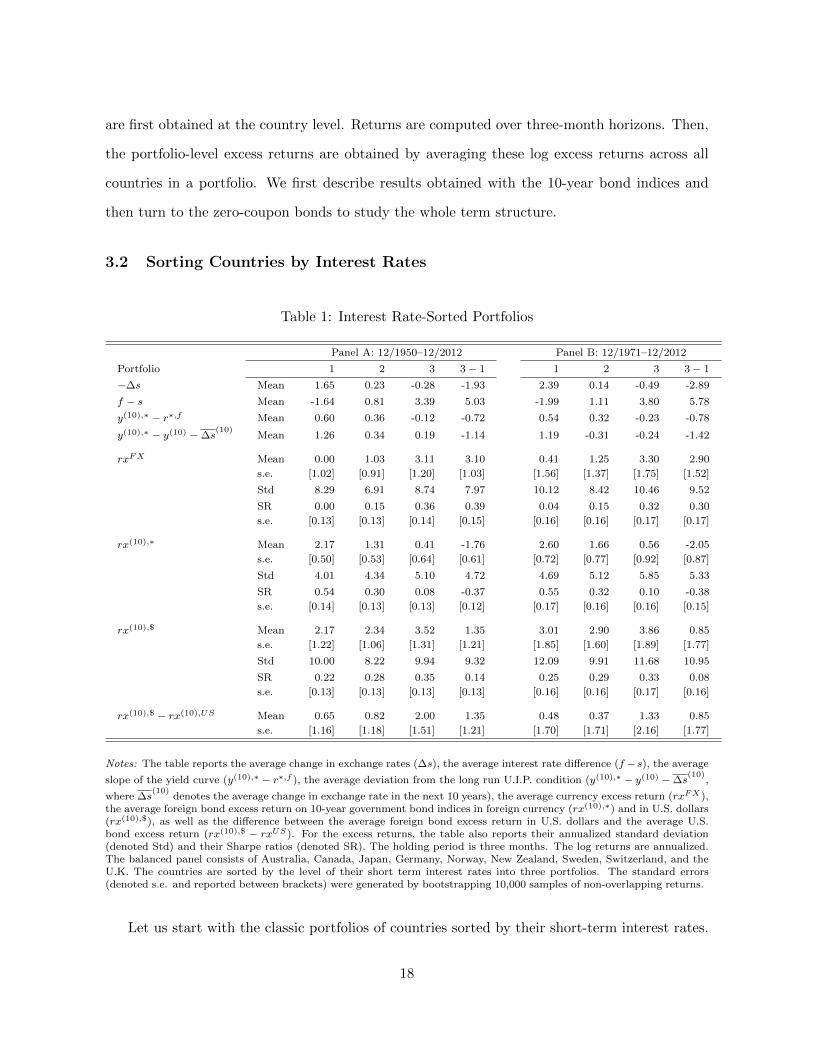
Table 1: Interest Rate-Sorted Portfolios

Panel A: 12/1950–12/2012 Panel B: 12/1971–12/2012

Portfolio 1 2 3 3− 1 1 2 3 3− 1

−∆s Mean 1.65 0.23 -0.28 -1.93 2.39 0.14 -0.49 -2.89

f − s Mean -1.64 0.81 3.39 5.03 -1.99 1.11 3.80 5.78

y(10),∗ − r∗,f Mean 0.60 0.36 -0.12 -0.72 0.54 0.32 -0.23 -0.78

y(10),∗ − y(10) −∆s(10)

Mean 1.26 0.34 0.19 -1.14 1.19 -0.31 -0.24 -1.42

rxFX Mean 0.00 1.03 3.11 3.10 0.41 1.25 3.30 2.90

s.e. [1.02] [0.91] [1.20] [1.03] [1.56] [1.37] [1.75] [1.52]

Std 8.29 6.91 8.74 7.97 10.12 8.42 10.46 9.52

SR 0.00 0.15 0.36 0.39 0.04 0.15 0.32 0.30

s.e. [0.13] [0.13] [0.14] [0.15] [0.16] [0.16] [0.17] [0.17]

rx(10),∗ Mean 2.17 1.31 0.41 -1.76 2.60 1.66 0.56 -2.05

s.e. [0.50] [0.53] [0.64] [0.61] [0.72] [0.77] [0.92] [0.87]

Std 4.01 4.34 5.10 4.72 4.69 5.12 5.85 5.33

SR 0.54 0.30 0.08 -0.37 0.55 0.32 0.10 -0.38

s.e. [0.14] [0.13] [0.13] [0.12] [0.17] [0.16] [0.16] [0.15]

rx(10),$ Mean 2.17 2.34 3.52 1.35 3.01 2.90 3.86 0.85

s.e. [1.22] [1.06] [1.31] [1.21] [1.85] [1.60] [1.89] [1.77]

Std 10.00 8.22 9.94 9.32 12.09 9.91 11.68 10.95

SR 0.22 0.28 0.35 0.14 0.25 0.29 0.33 0.08

s.e. [0.13] [0.13] [0.13] [0.13] [0.16] [0.16] [0.17] [0.16]

rx(10),$ − rx(10),US Mean 0.65 0.82 2.00 1.35 0.48 0.37 1.33 0.85

s.e. [1.16] [1.18] [1.51] [1.21] [1.70] [1.71] [2.16] [1.77]

Notes: The table reports the average change in exchange rates (∆s), the average interest rate difference (f −s), the average

slope of the yield curve (y(10),∗ − r∗,f ), the average deviation from the long run U.I.P. condition (y(10),∗ − y(10) −∆s(10)

,

where ∆s(10)

denotes the average change in exchange rate in the next 10 years), the average currency excess return (rxFX),the average foreign bond excess return on 10-year government bond indices in foreign currency (rx(10),∗) and in U.S. dollars(rx(10),$), as well as the difference between the average foreign bond excess return in U.S. dollars and the average U.S.bond excess return (rx(10),$ − rxUS). For the excess returns, the table also reports their annualized standard deviation(denoted Std) and their Sharpe ratios (denoted SR). The holding period is three months. The log returns are annualized.The balanced panel consists of Australia, Canada, Japan, Germany, Norway, New Zealand, Sweden, Switzerland, and theU.K. The countries are sorted by the level of their short term interest rates into three portfolios. The standard errors(denoted s.e. and reported between brackets) were generated by bootstrapping 10,000 samples of non-overlapping returns.

Let us start with the classic portfolios of countries sorted by their short-term interest rates.

18

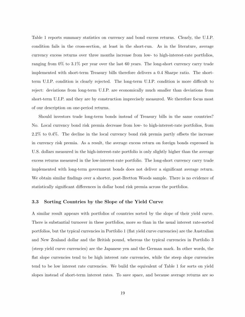
Table 1 reports summary statistics on currency and bond excess returns. Clearly, the U.I.P.

condition fails in the cross-section, at least in the short-run. As in the literature, average

currency excess returns over three months increase from low- to high-interest-rate portfolios,

ranging from 0% to 3.1% per year over the last 60 years. The long-short currency carry trade

implemented with short-term Treasury bills therefore delivers a 0.4 Sharpe ratio. The short-

term U.I.P. condition is clearly rejected. The long-term U.I.P. condition is more difficult to

reject: deviations from long-term U.I.P. are economically much smaller than deviations from

short-term U.I.P. and they are by construction imprecisely measured. We therefore focus most

of our description on one-period returns.

Should investors trade long-term bonds instead of Treasury bills in the same countries?

No. Local currency bond risk premia decrease from low- to high-interest-rate portfolios, from

2.2% to 0.4%. The decline in the local currency bond risk premia partly offsets the increase

in currency risk premia. As a result, the average excess return on foreign bonds expressed in

U.S. dollars measured in the high-interest-rate portfolio is only slightly higher than the average

excess returns measured in the low-interest-rate portfolio. The long-short currency carry trade

implemented with long-term government bonds does not deliver a significant average return.

We obtain similar findings over a shorter, post-Bretton Woods sample. There is no evidence of

statistically significant differences in dollar bond risk premia across the portfolios.

3.3 Sorting Countries by the Slope of the Yield Curve

A similar result appears with portfolios of countries sorted by the slope of their yield curve.

There is substantial turnover in these portfolios, more so than in the usual interest rate-sorted

portfolios, but the typical currencies in Portfolio 1 (flat yield curve currencies) are the Australian

and New Zealand dollar and the British pound, whereas the typical currencies in Portfolio 3

(steep yield curve currencies) are the Japanese yen and the German mark. In other words, the

flat slope currencies tend to be high interest rate currencies, while the steep slope currencies

tend to be low interest rate currencies. We build the equivalent of Table 1 for sorts on yield

slopes instead of short-term interest rates. To save space, and because average returns are so

19

similar, we report and comment all the results in the Appendix.

3.4 Looking Across Maturities

The previous results focus on the 10-year maturity. We now turn to the full maturity spectrum,

using the zero-coupon bond dataset.

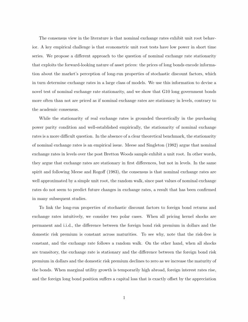
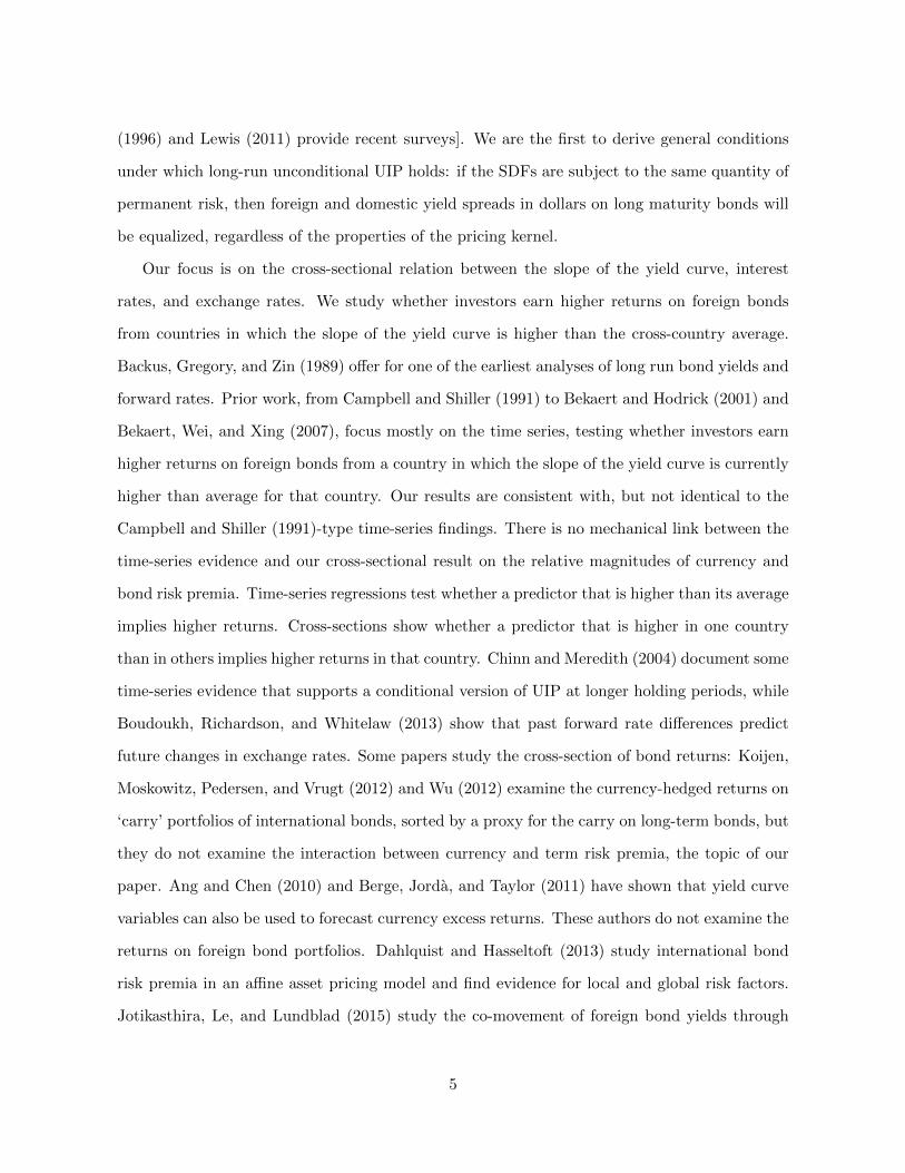
Figure 1 shows the dollar log excess returns as a function of the bond maturities, using the

same set of funding and investment currencies. Investing in short-term bills of countries with

flat yield curves (mostly high short-term interest rate) while borrowing at the same horizon

in countries with steep yield curves (mostly low short-term interest rate countries) leads to

positive excess returns on average (equal to 2.69%). This is the classic carry trade; its average

excess return is represented here on the left hand side of the graph. Investing and borrowing in

long-term bonds of the same countries, however, deliver negative insignificant excess returns on

average (equal to −1.77%). This is the carry trade at the long end of the term structure curve,

represented here on the right hand side of the graph. As the maturity of the bonds increases,

the average excess return decreases.

Foreign bond risk premia clearly differ across maturities: carry trade strategies that yield

positive risk premia for short-maturity bonds yield lower risk premia for long-maturity bonds.

3.5 Robustness Checks

We consider many robustness checks, studying (i) different time windows, (ii) different lengths

of the bond holding period, and (iii) different samples of countries. All the results are reported

in the Online Appendix. Here we simply describe the main findings.

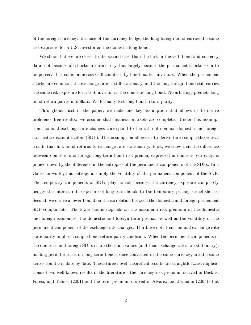
The results appear robust across time windows. Figure 2 presents the cumulative three-

month log returns on investments in foreign Treasury bills and foreign 10-year bonds, starting in

1950. Countries are sorted into portfolios based on the slope of their yield curves. The returns

correspond to an investment strategy going long in Portfolio 1 (flat yield curves, mostly high

short-term interest rates) and short in the Portfolio 3 (steep yield curves, mostly low short-term

interest rates). Even when dividing the sample into two, three, or four sub periods, the main

20

Dol

lar

Exc

ess

Ret

urns

Maturity (in quarters)5 10 15 20 25 30 35 40 45 50 55 60

−6

−4

−2

0

2

4

6

Figure 1: Long-Minus-Short Foreign Bond Risk Premia in U.S. Dollars— The figure shows the dollar logexcess returns as a function of the bond maturities. Dollar excess returns correspond to the holding period returns expressedin U.S. dollars of investment strategies that go long and short foreign bonds of different countries. The unbalanced panel ofcountries consists of Australia, Canada, Japan, Germany, Norway, New Zealand, Sweden, Switzerland, and the U.K. At eachdate t, the countries are sorted by the slope of their yield curves into three portfolios. The first portfolio contains countrieswith flat yield curves (mostly high interest rate) while the last portfolio contains countries with steep yield curves (mostlylow interest rate countries). The first portfolio correspond to the investment currencies while the third one corresponds tothe funding currencies. The slope of the yield curve is measured by the difference between the 10-year yield and the 3-monthinterest rate at date t. The holding period is one quarter. The returns are annualized. The shaded areas correspond toone standard deviation above and below each point estimate. Standard deviations are obtained by bootstrapping 10,000samples of non-overlapping returns. Zero-coupon data are monthly, and the sample window is 4/1985–12/2012.

result remains: an investor in short-term Treasury bills enjoys positive returns, while an investor

in long-term bonds of the same countries suffers negative returns. Again, currency and local

term premia offset each other, and thus average carry trade returns are different at the short-end

and the log end of the term structure.

The results appear robust to the choice of the bond holding period. We consider investments

of one, three, and twelve months. The patterns are similar. We sometimes obtain significant

dollar term premia when investors only invest for one month, but such a strategy would entail

21

1957 1971 1984 1998 2012

−6

−4

−2

0

2

4

The Slope Carry Trade

cu

mula

tive log r

etu

rns

FX Premium

Local Bond Premium

Figure 2: The Carry Trade and Term Premia: Conditional on the Slope of the Yield Curve –The figure presents the cumulative one-month log returns on investments in foreign Treasury bills and foreign10-year bonds. The benchmark panel of countries includes Australia, Canada, Japan, Germany, Norway, NewZealand, Sweden, Switzerland, and the U.K. Countries are sorted every month by the slope of their yield curvesinto three portfolios. The slope of the yield curve is measured by the spread between the 10-year bond yield andthe one-month interest rate. The returns correspond to an investment strategy going long in Portfolio 1 and shortin the Portfolio 3. The sample period is 12/1950–12/2012.

large transaction costs, which would likely wipe out the returns. For longer holding periods, the

dollar term premia are not significant.

The results appear also robust across several samples of countries.10 For each dataset, we

10With discount bonds, we consider two additional sets of countries: first, a larger sample of 20 developedcountries (Australia, Austria, Belgium, Canada, Denmark, Finland, France, Germany, Greece, Ireland, Italy,Japan, the Netherlands, New Zealand, Norway, Portugal, Spain, Sweden, Switzerland, and the U.K.), and sec-ond, a large sample of 30 developed and emerging countries (the same as above, plus India, Mexico, Malaysia,the Netherlands, Pakistan, the Philippines, Poland, South Africa, Singapore, Taiwan, and Thailand). We alsoconstruct an extended version of the zero-coupon dataset which, in addition to the countries of the benchmarksample, includes the following countries: Austria, Belgium, the Czech Republic, Denmark, Finland, France, Hun-gary, Indonesia, Ireland, Italy, Malaysia, Mexico, the Netherlands, Poland, Portugal, Singapore, South Africa,and Spain. The data for the aforementioned extra countries are sourced from Bloomberg. The starting dates for

22

report and comment detailed results over the full time-window and the post-Bretton-Woods

sample. Since the results are similar to those in our benchmark sample, they are reported in

the Online Appendix.

3.6 Finite- vs Infinite-Maturity Bond Returns

Before turning to time-series tests of the bond return parity, we pause to stress a key difference

between our theoretical and empirical work. Our empirical results pertain to 10- and 15-year

bond returns while our theoretical results pertain to infinite-maturity bonds. How do we know

that our theory is empirically relevant?

To address this question, we use the state-of-the-art Joslin, Singleton, and Zhu (2011) term

structure model to study empirically the difference between the 10-year and infinite-maturity

bonds in each country of our G10 sample. Estimation and simulation results are reported in

the Online Appendix. We ignore the simulated data for Australia, Canada, New Zealand and

Sweden as the parameter estimates imply there that the yield curves turn negative on long

maturities; we focus instead on Germany, Japan, Norway, Switzerland, U.K., and U.S. We

study both unconditional and conditional returns, forming portfolios of countries sorted by the

level or slope of their yield curves, as we did in the data. Infinite maturity bond returns appear

larger than their 10-year counterparts on average, but not significantly so in small samples. The

correlation between the 10-year and infinite maturity bonds are high, both at the country- and

at the portfolio-level.

In theory, it is certainly possible to write a model where the 10-year bond returns, once

expressed in the same currency, offer similar average returns across countries — as we find

in the data, while the infinite maturity bonds do not. In that case, there would be a gap

between our theory and the data. In such a model, however, exchange rates would have unit

root components driven by common shocks and the cross-sectional distribution of exchange rates

would fan out over time. For developing countries with strong trade links and similar inflation

the additional countries are as follows: 12/1994 for Austria, Belgium, Denmark, Finland, France, Ireland, Italy,the Netherlands, Portugal, Singapore, and Spain, 12/2000 for the Czech Republic, 3/2001 for Hungary, 5/2003for Indonesia, 9/2001 for Malaysia, 8/2003 for Mexico, 12/2000 for Poland, and 1/1995 for South Africa.

23

rates, this seems hard to defend. Moreover, although we cannot rule out its existence, we do not

know of such a model. In the state-of-the-art of the term structure modeling, our inference about

infinite-maturity bonds from 10-year bonds is reasonable. We thus proceed to study further the

link between exchange rate stationarity and bond returns.

4 Time-Series Tests of the Uncovered Bond Return Parity

In this section, we first show that the permanent components of the SDFs are highly correlated.

Then we test whether they are the same over 60-month rolling windows using the uncovered

bond return parity condition.

4.1 The Correlation of the Permanent Components of the SDFs

Since exchange rate changes and their temporary components are observable (thanks to the

bonds’ holding period returns), one can compute the variance of the permanent component of

exchange rates, var(

logSPt+1

SPt

). In the data; the contribution of the last term is on the order

of 1% or less. Given the large size of the equity premium compared to the term premium (a

7.5% difference according to Alvarez and Jermann, 2005), and the relatively small variance of

the permanent component of exchange rates, the lower bound in Proposition 2 implies a large

correlation of the permanent components.

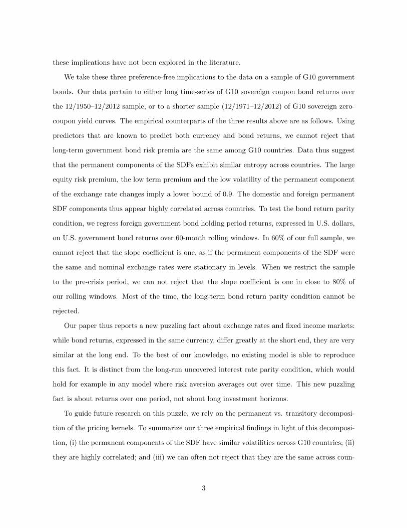
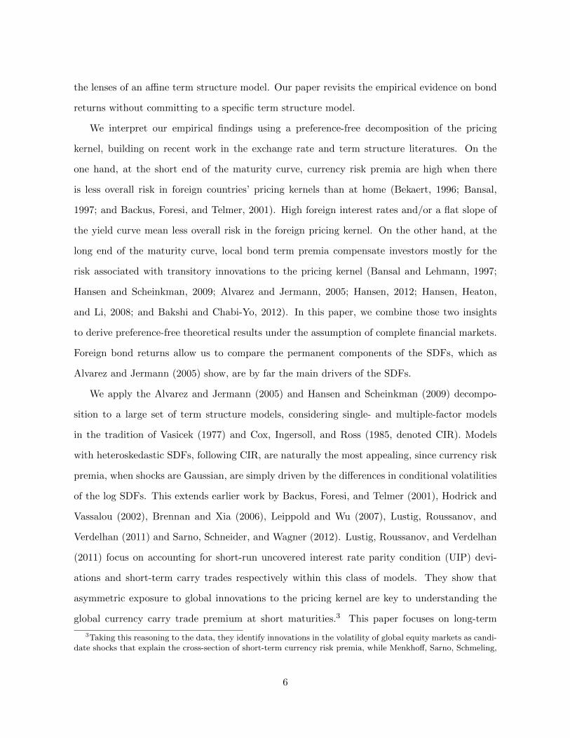
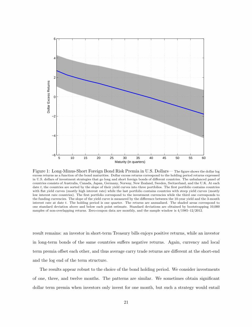
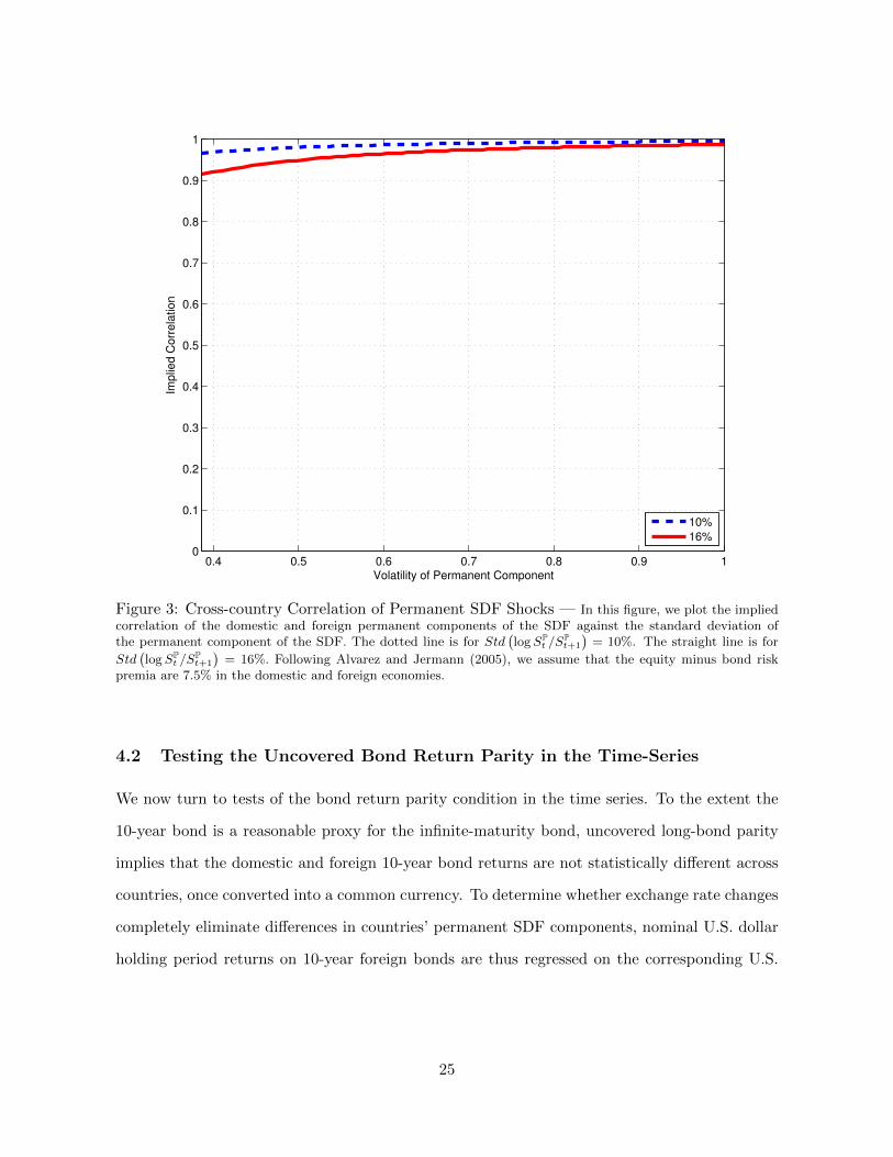
In Figure 3, we plot the implied correlation of the permanent component against the volatility

of the permanent component in the symmetric case for two different scenarios. The dotted line

is for Std(logSP

t /SPt+1

)= 10%, and the plain line is for Std

(logSP

t /SPt+1

)= 16%. In both cases,

the implied correlation of the permanent components of the domestic and foreign pricing kernels

is clearly above 0.9.

While Brandt, Cochrane, and Santa-Clara (2006) find that the SDFs are highly correlated

across countries, we find that the permanent components of the SDFs, which are the main

sources of volatility for the SDFs, are highly correlated across countries. Simple regression tests

allow us to go further.

24

0.4 0.5 0.6 0.7 0.8 0.9 10

0.1

0.2

0.3

0.4

0.5

0.6

0.7

0.8

0.9

1

Volatility of Permanent Component

Implie

d C

orr

ela

tion

10%

16%

Figure 3: Cross-country Correlation of Permanent SDF Shocks — In this figure, we plot the impliedcorrelation of the domestic and foreign permanent components of the SDF against the standard deviation ofthe permanent component of the SDF. The dotted line is for Std

(logSP

t /SPt+1

)= 10%. The straight line is for

Std(logSP

t /SPt+1

)= 16%. Following Alvarez and Jermann (2005), we assume that the equity minus bond risk

premia are 7.5% in the domestic and foreign economies.

4.2 Testing the Uncovered Bond Return Parity in the Time-Series

We now turn to tests of the bond return parity condition in the time series. To the extent the

10-year bond is a reasonable proxy for the infinite-maturity bond, uncovered long-bond parity

implies that the domestic and foreign 10-year bond returns are not statistically different across

countries, once converted into a common currency. To determine whether exchange rate changes

completely eliminate differences in countries’ permanent SDF components, nominal U.S. dollar

holding period returns on 10-year foreign bonds are thus regressed on the corresponding U.S.

25

dollar returns on 10-year U.S. bonds:

r(10),$t+1 = α+ βr

(10)t+1 + εt+1, (15)

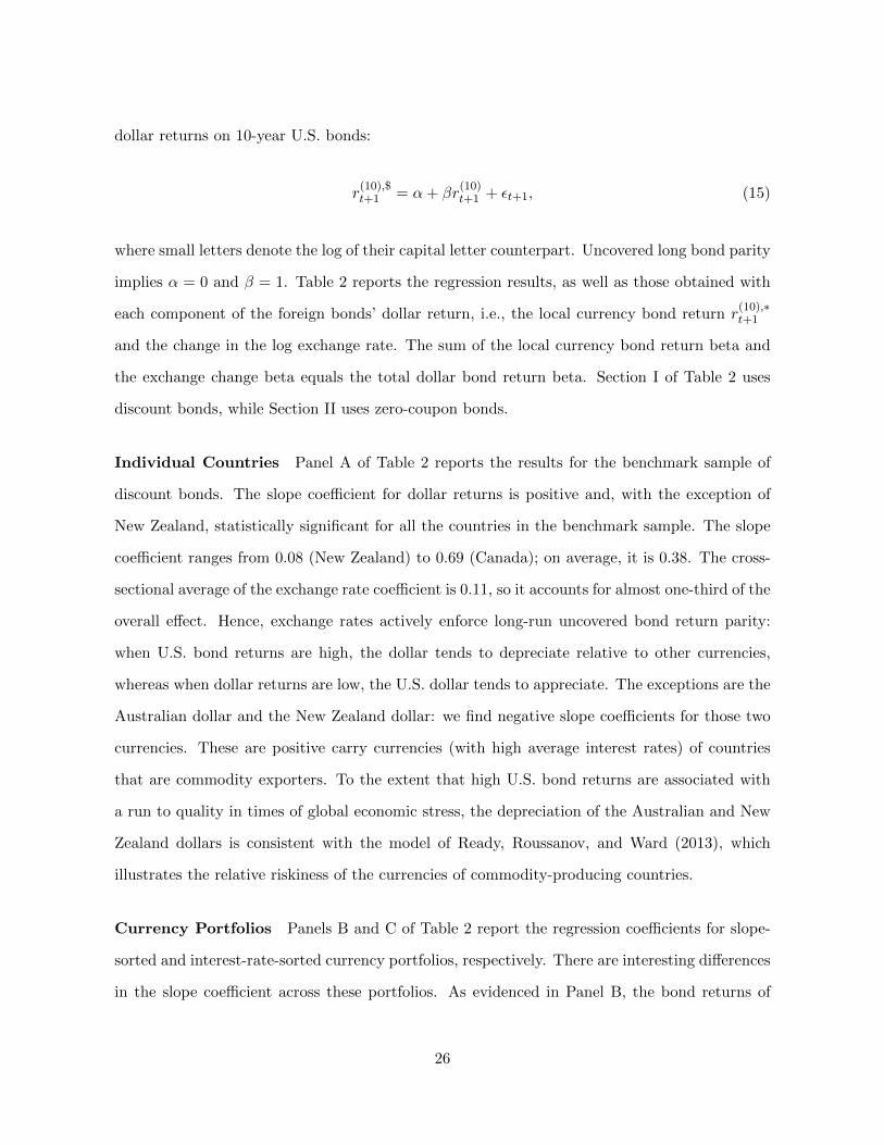
where small letters denote the log of their capital letter counterpart. Uncovered long bond parity

implies α = 0 and β = 1. Table 2 reports the regression results, as well as those obtained with

each component of the foreign bonds’ dollar return, i.e., the local currency bond return r(10),∗t+1

and the change in the log exchange rate. The sum of the local currency bond return beta and

the exchange change beta equals the total dollar bond return beta. Section I of Table 2 uses

discount bonds, while Section II uses zero-coupon bonds.

Individual Countries Panel A of Table 2 reports the results for the benchmark sample of

discount bonds. The slope coefficient for dollar returns is positive and, with the exception of

New Zealand, statistically significant for all the countries in the benchmark sample. The slope

coefficient ranges from 0.08 (New Zealand) to 0.69 (Canada); on average, it is 0.38. The cross-

sectional average of the exchange rate coefficient is 0.11, so it accounts for almost one-third of the

overall effect. Hence, exchange rates actively enforce long-run uncovered bond return parity:

when U.S. bond returns are high, the dollar tends to depreciate relative to other currencies,

whereas when dollar returns are low, the U.S. dollar tends to appreciate. The exceptions are the

Australian dollar and the New Zealand dollar: we find negative slope coefficients for those two

currencies. These are positive carry currencies (with high average interest rates) of countries

that are commodity exporters. To the extent that high U.S. bond returns are associated with

a run to quality in times of global economic stress, the depreciation of the Australian and New

Zealand dollars is consistent with the model of Ready, Roussanov, and Ward (2013), which

illustrates the relative riskiness of the currencies of commodity-producing countries.

Currency Portfolios Panels B and C of Table 2 report the regression coefficients for slope-

sorted and interest-rate-sorted currency portfolios, respectively. There are interesting differences

in the slope coefficient across these portfolios. As evidenced in Panel B, the bond returns of

26

countries with flat yield curves have lower dollar betas than the returns of steep yield curve

countries. Furthermore, Panel C reveals that the long-maturity bond returns of low interest rate

countries comove more with U.S. bond returns than the returns of high interest rate countries.

To check the robustness of our results, we run the bond return parity regressions on zero-

coupon bonds. The results are reported in the Section II of Table 2. They are broadly consistent

with the previous findings. Specifically, the cross-sectional average of the dollar return slope is

0.61, implying significant comovement between foreign and U.S. dollar bond returns. This is due

to the fact that the dataset is biased towards the recent period, when dollar betas are historically

high.

Overall, the long-run uncovered bond parity condition appears a better fit in the cross-section

on average than in the time series. We can largely reject that the slope coefficients are zero, but

we can also reject (although by a much smaller margin) that the bond parity condition holds

unconditionally in the time-series. These unconditional slope coefficients, however, hide large

time-variations.

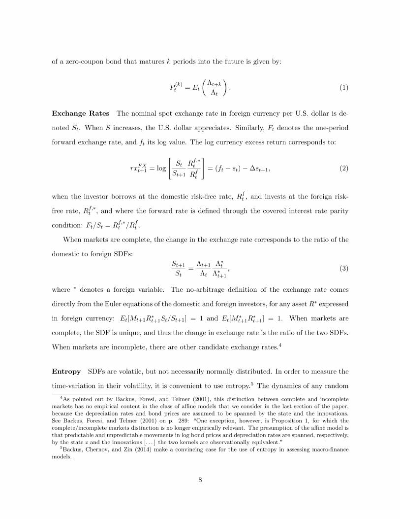
Time Variation To study the time-variation in the regression coefficients, we run the same

regressions but on 60-month rolling windows of zero-coupon 10-year bond returns. Figure 4

reports the slope coefficients for each G10 country, along with shaded areas that represent two

standard errors around the point estimates.

For 61% of the rolling windows, we cannot reject that the slope coefficient is equal to one

and thus we cannot reject that the bond return parity holds. Over the different countries, this

percentage varies from a minimum of 47% to a maximum of 79%. This result is surprising.

Under the assumption that markets are complete and that 10-year bond returns proxy for long-

term bond returns, the bond return parity holds when nominal exchange rates are stationary in

levels. The academic consensus is that nominal exchange rates are stationary in first differences,

but not in levels. In almost two-thirds of the rolling windows, the bond market behaves as if

nominal exchange rates were stationary in levels.

When we restrict the sample to the pre-crisis period (thus ending in December 2006), the

results are even stronger. For 78% of the rolling windows, we cannot reject that the slope

27

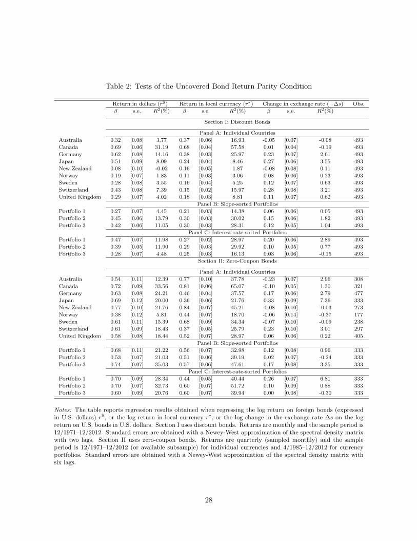
Table 2: Tests of the Uncovered Bond Return Parity Condition

Return in dollars (r$) Return in local currency (r∗) Change in exchange rate (−∆s) Obs.

β s.e. R2(%) β s.e. R2(%) β s.e. R2(%)

Section I: Discount Bonds

Panel A: Individual Countries

Australia 0.32 [0.08] 3.77 0.37 [0.06] 16.93 -0.05 [0.07] -0.08 493

Canada 0.69 [0.06] 31.19 0.68 [0.04] 57.58 0.01 [0.04] -0.19 493

Germany 0.62 [0.08] 14.16 0.38 [0.03] 25.97 0.23 [0.07] 2.61 493

Japan 0.51 [0.09] 8.09 0.24 [0.04] 8.46 0.27 [0.06] 3.55 493

New Zealand 0.08 [0.10] -0.02 0.16 [0.05] 1.87 -0.08 [0.08] 0.11 493

Norway 0.19 [0.07] 1.83 0.11 [0.03] 3.06 0.08 [0.06] 0.23 493

Sweden 0.28 [0.08] 3.55 0.16 [0.04] 5.25 0.12 [0.07] 0.63 493

Switzerland 0.43 [0.08] 7.39 0.15 [0.02] 15.97 0.28 [0.08] 3.21 493

United Kingdom 0.29 [0.07] 4.02 0.18 [0.03] 8.81 0.11 [0.07] 0.62 493

Panel B: Slope-sorted Portfolios

Portfolio 1 0.27 [0.07] 4.45 0.21 [0.03] 14.38 0.06 [0.06] 0.05 493

Portfolio 2 0.45 [0.06] 13.79 0.30 [0.03] 30.02 0.15 [0.06] 1.82 493

Portfolio 3 0.42 [0.06] 11.05 0.30 [0.03] 28.31 0.12 [0.05] 1.04 493

Panel C: Interest-rate-sorted Portfolios

Portfolio 1 0.47 [0.07] 11.98 0.27 [0.02] 28.97 0.20 [0.06] 2.89 493

Portfolio 2 0.39 [0.05] 11.90 0.29 [0.03] 29.92 0.10 [0.05] 0.77 493

Portfolio 3 0.28 [0.07] 4.48 0.25 [0.03] 16.13 0.03 [0.06] -0.15 493

Section II: Zero-Coupon Bonds

Panel A: Individual Countries

Australia 0.54 [0.11] 12.39 0.77 [0.10] 37.78 -0.23 [0.07] 2.96 308

Canada 0.72 [0.09] 33.56 0.81 [0.06] 65.07 -0.10 [0.05] 1.30 321

Germany 0.63 [0.08] 24.21 0.46 [0.04] 37.57 0.17 [0.06] 2.79 477

Japan 0.69 [0.12] 20.00 0.36 [0.06] 21.76 0.33 [0.09] 7.36 333

New Zealand 0.77 [0.10] 21.76 0.84 [0.07] 45.21 -0.08 [0.10] -0.03 273

Norway 0.38 [0.12] 5.81 0.44 [0.07] 18.70 -0.06 [0.14] -0.37 177

Sweden 0.61 [0.11] 15.39 0.68 [0.09] 34.34 -0.07 [0.10] -0.09 238

Switzerland 0.61 [0.09] 18.43 0.37 [0.05] 25.79 0.23 [0.10] 3.01 297

United Kingdom 0.58 [0.08] 18.44 0.52 [0.07] 28.97 0.06 [0.06] 0.22 405

Panel B: Slope-sorted Portfolios

Portfolio 1 0.68 [0.11] 21.22 0.56 [0.07] 32.98 0.12 [0.08] 0.96 333

Portfolio 2 0.53 [0.07] 21.03 0.51 [0.06] 39.19 0.02 [0.07] -0.24 333

Portfolio 3 0.74 [0.07] 35.03 0.57 [0.06] 47.61 0.17 [0.08] 3.35 333

Panel C: Interest-rate-sorted Portfolios

Portfolio 1 0.70 [0.09] 28.34 0.44 [0.05] 40.44 0.26 [0.07] 6.81 333

Portfolio 2 0.70 [0.07] 32.73 0.60 [0.07] 51.72 0.10 [0.09] 0.88 333

Portfolio 3 0.60 [0.09] 20.76 0.60 [0.07] 39.94 0.00 [0.08] -0.30 333

Notes: The table reports regression results obtained when regressing the log return on foreign bonds (expressedin U.S. dollars) r$, or the log return in local currency r∗, or the log change in the exchange rate ∆s on the logreturn on U.S. bonds in U.S. dollars. Section I uses discount bonds. Returns are monthly and the sample period is12/1971–12/2012. Standard errors are obtained with a Newey-West approximation of the spectral density matrixwith two lags. Section II uses zero-coupon bonds. Returns are quarterly (sampled monthly) and the sampleperiod is 12/1971–12/2012 (or available subsample) for individual currencies and 4/1985–12/2012 for currencyportfolios. Standard errors are obtained with a Newey-West approximation of the spectral density matrix withsix lags.

28

Australia

1995 2000 2005 2010

0

0.5

1

Canada

1995 2000 2005 2010

0

0.5

1

Germany

1990 2000 2010

0

0.5

1

Japan

1995 2000 2005 2010

0

0.5

1

New Zealand

2000 2005 2010

0

0.5

1

Norway

2005 2007 2010 2012

0

0.5

1

Sweden

2000 2005 2010

0

0.5

1

Switzerland

1995 2000 2005 2010

0

0.5

1

United Kingdom

1990 2000 2010

0

0.5

1

Figure 4: Foreign Bond Return Betas — This figure presents the 60-month rolling window estimation of foreignbond betas with respect to U.S. bond holding period returns for each G10 country. The holding period is three months.The sample is 4/1985–12/2012. The shaded areas represent two standard errors around the point estimates. Standarderrors are obtained by bootstrapping.

coefficient is equal to one. Over the different countries, this percentage varies from a minimum

of 57% to a maximum of 100%. The crisis and post-crisis periods are characterized by large

deviations from arbitrage opportunities, which may explain deviations from the long-term bond

return parity condition. In the pre-crisis period, this condition appears like a natural benchmark.

Building on our theoretical and empirical results, we now derive necessary conditions in a

large class of affine term structure models that need to be satisfied in order to simultaneously

produce large currency carry trade risk premia and no long-term bond risk premia differences

across countries.

29

5 Implications for Affine Term Structure Models

In this section, we derive parametric restrictions for affine term structure models that imply

zero carry trade risk premia at long maturities. These sufficient conditions for zero carry trade

risk premia at long horizons also rule out non-stationarity of the nominal exchange rate.

For the sake of clarity, we focus on the classic Cox, Ingersoll, and Ross (1985) model in

the main text. In the Online Appendix, we cover a wide range of term structure models,

from the seminal Vasicek (1977) model and to the most recent, multi-factor dynamic term

structure models. All the proofs are in the Online Appendix; there we also show that the

operator- and eigenfunction-based approach of Hansen and Scheinkman (2009) delivers the same

decomposition as the Alvarez and Jermann (2005) approach. For each of these models, we first

analyze specifications with country-specific factors and then to turn to global factors that are

common across countries. Carry trade risk premia arise from asymmetric exposures to global

factors. If the entropy of the permanent component cannot differ across countries, then all

countries’ pricing kernels need the same loadings on the permanent component of the global

factors.

In the Cox, Ingersoll, and Ross (1985) model (denoted CIR), the stochastic discount factor

evolves according to:

− logMt+1 = α+ χzt +√γztut+1, ut+1 ∼ N (0, 1) (16)

zt+1 = (1− φ)θ + φzt − σ√ztut+1. (17)

In the CIR model, log bond prices are also affine in the state variable z: p(n)t = −Bn

0 − Bn1 zt,

where Bn0 and Bn

1 are the solution to difference equations.11 The temporary and martingale

11The bond price coefficients evolve according to the following second-order difference equations:

Bn0 = α+Bn−10 +Bn−1

1 (1− φ)θ,

Bn1 = χ− 1

2γ +Bn−1

1 φ− 1

2

(Bn−1

1

)2σ2 + σ

√γBn−1

1 .

30

components of the SDF are:

ΛTt = lim

n→∞

βt+n

P(n)t

= limn→∞

βt+neBn0 +Bn1 zt , (18)

ΛPt+1

ΛPt

=Λt+1

Λt

(ΛTt+1

ΛTt

)−1

= β−1e−α−χzt−√γztut+1e−B

∞1 [(φ−1)(zt−θ)−σ

√ztut+1]. (19)

where the constant β = e−α−B∞1 (1−φ)θ is chosen to offset the growth in Bn

0 as n becomes very

large. The expected log excess return of an infinite maturity bond is then:

Et

[rx

(∞)t+1

]= [B∞1 (1− φ)− χ+ γ/2] zt, (20)

where B∞1 is defined implicitly in the following second-order equation: B∞1 = χ− γ/2 +B∞1 φ−

(B∞1 )2 σ2/2 + σ√γB∞1 .

Model with Country-specific Factors Suppose that the foreign pricing kernel is specified

as above with the same parameters. The foreign country has its own factor z∗.

− logM∗t+1 = α+ χz∗t +√γz∗t u

∗t+1, (21)

z∗t+1 = (1− φ)θ + φz∗t − σ√z∗t u∗t+1. (22)

The foreign innovations u∗t+1 are not correlated with their domestic counterparts ut+1. The log

currency risk premium is given by Et[rxFXt+1] = 1

2γ(zt − z∗t ).

Result 1. In a symmetric CIR model (i.e., when countries share the same parameters) with

country-specific factors, the long bond uncovered return parity condition holds only if the model

parameters satisfy the following restriction: χ/(1− φ) =√γ/σ.

In the CIR model, there are no permanent innovations to the pricing kernel provided that

B∞1 = χ1−φ . In this case, the second-order equation that defines B∞1 implies B∞1 =

√γ/σ. This

condition insures that the price of the long bond fully absorbs the cumulative impact of the

innovations on the level of the pricing kernel. As a result, the permanent component of the

31

pricing kernel is constant:ΛPt+1

ΛPt

= β−1e−α−χθ. The term premium on the infinite maturity bond

in Equation (20) reduces to (1/2)γzt, the maximum log risk premium.

In the absence of a permanent component, the expected foreign log holding period return on

a foreign long bond converted into U.S. dollars is equal to the U.S. term premium: 12γzt. The

nominal exchange rate has no permanent component(SPt /S

Pt+1 = 1

), and hence is stationary.

Model with Global Factor Next, we consider a model in which zt = z∗t is a single global

state variable that drives the pricing kernel in all countries. The model is thus:

− logMt+1 = α+ χzt +√γztut+1, (23)

− logM∗t+1 = α∗ + χ∗zt +√γ∗ztut+1, (24)

zt+1 = (1− φ)θ + φzt − σ√ztut+1. (25)

Result 2. In a CIR model with a global factor subject to permanent shocks, the long bond

uncovered return parity condition holds only if the countries share the same parameters γ and

χ.

To understand this result, note that B∞1 depends on χ and γ, as well as on the global

parameters φ and σ. A necessary and sufficient condition is then the symmetry of the parameters

that govern global exposure: γ = γ∗ and χ = χ∗. Under these conditions, the domestic and

foreign pricing kernels react similarly to changes in the global “permanent ” state variable and its

innovations: the permanent component of the pricing kernel is common, the nominal exchange

rate has no permanent component(SPt /S

Pt+1 = 1

), and it is stationary.

The long-term bond return parity condition therefore imposes clear restrictions on cross-

country term structure models. These restrictions matter. To check this, we simulate a cali-

brated example of the N -country model developed by Lustig, Roussanov, and Verdelhan (2014)

to match the cross-sectional evidence in the currency portfolios. The model does not satisfy the

long term bond parity condition. The decomposition of the SDF shows why the model fails and

why it cannot be fixed with only one source of heterogeneity. All the results are reported in the

32

Online Appendix.

The key take-away from the study of term structure models is that the carry trade at the

short end of the yield curve must compensate investors for bearing global, temporary risks. This

result appears in different term structure models, and the intuition is simple. To generate carry

trade risk premia, countries’ pricing kernels need to have asymmetric exposures to global shocks

(Lustig, Roussanov, and Verdelhan, 2011). However, these global shocks cannot have permanent

effects. If they do, the models will generate counterfactual long-term carry premia as well.

6 Conclusion

This paper presents a simple but puzzling fact: while holding period bond returns, expressed

in a common currency, differ across G10 countries at the short end of the yield curve, they are

rather similar at the long end. To help explain this fact, we derive three simple preference-free

results that link the properties of SDFs and exchange rates to the foreign bond returns under

the assumption that markets are complete. Assuming that 10- and 15-year bond returns are

reasonable proxy for long-term bond returns, we cannot reject that the permanent components

of the SDFs exhibit the same volatility across G10 countries. Moreover, they appear highly

correlated. Over rolling-window regression tests, we can often not reject that the domestic

and foreign permanent components are the same. These findings suggest that the international

bond markets often view nominal exchange rates as stationary, contrary to the current academic

consensus.

33

References

Alvarez, F., A. Atkeson, and P. Kehoe (2002): “Money, Interest Rates and Exchange Rates

with Endogenously Segmented Markets,” Journal of Political Economy, 110(1), 73–112.

(2009): “Time-Varying Risk, Interest Rates and Exchange Rates in General Equilib-

rium,” Review of Economic Studies, 76, 851 – 878.

Alvarez, F., and U. J. Jermann (2005): “Using Asset Prices to Measure the Persistence of

the Marginal Utility of Wealth,” Econometrica, 73(6), 1977–2016.

Ang, A., and J. S. Chen (2010): “Yield Curve Predictors of Foreign Exchange Returns,”

Working Paper, Columbia University.

Backus, D., M. Chernov, and S. Zin (2014): “Sources of entropy in representative agent

models,” Journal of Finance, 69 (1), 51–99.

Backus, D., S. Foresi, and C. Telmer (2001): “Affine Models of Currency Pricing: Ac-

counting for the Forward Premium Anomaly,” Journal of Finance, 56, 279–304.

Backus, D. K., A. W. Gregory, and S. E. Zin (1989): “Risk premiums in the term

structure: Evidence from artificial economies,” Journal of Monetary Economics, 24(3), 371 –

399.

Bakshi, G., and F. Chabi-Yo (2012): “Variance bounds on the permanent and transitory

components of stochastic discount factors,” Journal of Financial Economics, 105, 191–208.

Bansal, R. (1997): “An Exploration of the Forward Premium Puzzle in Currency Markets,”

Review of Financial Studies, 10, 369–403.

Bansal, R., and B. N. Lehmann (1997): “Growth Optimal Portfolio Restrictions on Asset

Pricing Models,” Macroeconomic Dynamics, 1, 333–354.

Bekaert, G. (1996): “The Time Variation of Risk and Return in Foreign Exchange Markets:

A General Equilibrium Perspective,” The Review of Financial Studies, 9(2), 427–470.

34

Bekaert, G., and R. J. Hodrick (2001): “Expectations Hypotheses Tests,” The Journal of

Finance, 56(4), 1357–1394.

Bekaert, G., M. Wei, and Y. Xing (2007): “Uncovered interest rate parity and the term

structure,” Journal of International Money and Finance, 26(6), 1038 – 1069.

Berge, T. J., O. Jorda, and A. M. Taylor (2011): Currency Carry Trades, NBER Inter-

national Seminar on Macroeconomics 2010. University of Chicago Press.

Boudoukh, J., M. Richardson, and R. F. Whitelaw (2013): “New Evidence on the

Forward Premium Puzzle,” Journal of Financial and Quantitative Analysis, forthcoming.

Brandt, M. W., J. H. Cochrane, and P. Santa-Clara (2006): “International Risk Shar-

ing is Better Than You Think, or Exchange Rates are Too Smooth,” Journal of Monetary

Economics, 53(4), 671 – 698.

Brennan, M. J., and Y. Xia (2006): “International Capital Markets and Foreign Exchange

Risk,” Review of Financial Studies, 19(3), 753–795.

Brunnermeier, M. K., S. Nagel, and L. H. Pedersen (2009): “Carry Trades and Currency

Crashes,” NBER Macroeconomics Annual 2008, 23, 313–347.

Campbell, J. Y., and R. J. Shiller (1991): “Yield Spreads and Interest Rate Movements:

A Bird’s Eye View,” Review of Economic Studies, 58, 495–514.

Chabi-Yo, F., and R. Colacito (2015): “The Term Structures of Co-Entropy in International

Financial Markets,” Working Paper, Ohio State University.

Chernov, M., J. Graveline, and I. Zviadadze (2011): “Sources of Risk in Currency Re-

turns,” Working Paper, London School of Economics.

Chinn, M. D., and G. Meredith (2004): “Monetary Policy and Long-Horizon Uncovered

Interest Parity,” IMF Staff Papers, 51(3), 409–430.

Cochrane, J. H. (1988): “How Big Is the Random Walk in GNP?,” Journal of Political

Economy, 96(5), pp. 893–920.

35

Coeurdacier, N., H. Rey, and P. Winant (2013): “Financial Integration and Growth in a

Risky World,” Working Paper, London Business School.

Colacito, R., and M. M. Croce (2011): “Risks for the Long Run and the Real Exchange

Rate,” Journal of Political Economy, 119(1), 153–181.

Cole, H. L., and M. Obstfeld (1991): “Commodity Trade and International Risk Sharing:

How Much Do Financial Markets Matter?,” Journal of Monetary Economics, 28(1), 3–24.

Cox, J. C., J. E. Ingersoll, and S. A. Ross (1985): “A Theory of the Term Structure of

Interest Rates,” Econometrica, 53(2), 385–408.

Dahlquist, M., and H. Hasseltoft (2013): “International Bond Risk Premia,” Journal of

International Economics, 90, 12–32.

Didier, T., R. Rigobon, and S. L. Schmukler (2013): “Unexploited gains from international

diversification: Patterns of portfolio holdings around the world,” Review of Economics and

Statistics, 95 (5), 1562–1583.

Engel, C. (1996): “The Forward Discount Anomaly and the Risk Premium: A Survey of

Recent Evidence,” Journal of Empirical Finance, 3, 123–192.

Farhi, E., S. P. Fraiberger, X. Gabaix, R. Ranciere, and A. Verdelhan (2013):

“Crash Risk in Currency Markets,” Working Paper, Harvard University.

Gavazzoni, F., B. Sambalaibat, and C. Telmer (2012): “Currency Risk and Pricing Kernel

Volatility,” Working Paper, Carnegie Mellon University.

Gourinchas, P.-O., and O. Jeanne (2006): “The Elusive Gains from International Financial

Integration,” The Review of Economic Studies, 73(3), 715–741.

Gourio, F., M. Siemer, and A. Verdelhan (2013): “International Risk Cycles,” Journal of

International Economics, 89, 471–484.

Graveline, J. J., and S. Joslin (2011): “G10 Swap and Exchange Rates,” Working paper.

36

Hansen, L. P. (2012): “Dynamic Valuation Decomposition Within Stochastic Economies,”

Econometrica, 80 (3), 911–967.

Hansen, L. P., J. C. Heaton, and N. Li (2008): “Consumption Strikes Back? Measuring

Long-Run Risk,” Journal of Political Economy, 166(2), 260–302.

Hansen, L. P., and J. A. Scheinkman (2009): “Long-Term Risk: An Operator Approach,”

Econometrica, 77(1), 177–234.

Hodrick, R. J., and M. Vassalou (2002): “Do we need multi-country models to explain

exchange rate and interest rate and bond return dynamics?,” Journal of Economic Dynamics

and Control, 26, 1275–1299.

Joslin, S., K. J. Singleton, and H. Zhu (2011): “A new perspective on Gaussian dynamic

term structure models,” Review of Financial Studies, 24(3), 926–970.

Jotikasthira, C., A. Le, and C. Lundblad (2015): “Why do term structures in different

currencies co-move?,” Journal of Financial Economics, 115(1), 58 – 83.

Jurek, J. W. (2014): “Crash-neutral Currency Carry Trades,” Journal of Financial Economics,

113(3), 325 – 347.

Koijen, R., T. J. Moskowitz, L. H. Pedersen, and E. B. Vrugt (2012): “Carry,” Working

Paper, University of Chicago.

Leippold, M., and L. Wu (2007): “Design and Estimation of Multi-Currency Quadratic

Models,” Review of Finance, 11(2), 167–207.

Lewis, K. K. (2000): “Why Do Stocks and Consumption Imply Such Different Gains From

International Risk-Sharing?,” Journal of International Economics, 52(1), 1–35.

Lewis, K. K. (2011): “Global Asset Pricing,” Annual Review of Financial Economics.

Lewis, K. K., and E. X. Liu (2012): “Evaluating International Consumption Risk Sharing

Gains: An Asset Return View,” Working Paper, University of Pennsylvania.

37

Lustig, H., N. Roussanov, and A. Verdelhan (2011): “Common Risk Factors in Currency

Returns,” Review of Financial Studies, 24(11).

(2014): “Countercyclical currency risk premia,” Journal of Financial Economics,

111(3), 527–553.

Lustig, H., and A. Verdelhan (2007): “The Cross-Section of Foreign Currency Risk Premia

and Consumption Growth Risk,” American Economic Review, 97(1), 98–117.

(2015): “Does Incomplete Spanning in International Financial Markets Help to Explain

Exchange Rates?,” Working Paper, Stanford University and MIT.

Martin, I., and S. A. Ross (2013): “The Long Bond,” Working Paper, Stanford University.

Meese, R. A., and K. J. Singleton (1982): “On unit roots and the empirical modeling of

exchange rates,” the Journal of Finance, 37(4), 1029–1035.

Menkhoff, L., L. Sarno, M. Schmeling, and A. Schrimpf (2012): “Carry Trades and

Global FX Volatility,” Journal of Finance, 67(2), 681–718.

Meredith, G., and M. D. Chinn (2005): “Testing Uncovered Interest Rate Parity at Short

and Long Horizons during the Post-Bretton Woods Era,” Working Paper NBER 11077.

Ready, R. C., N. L. Roussanov, and C. Ward (2013): “Commodity Trade and the Carry

Trade: A Tale of Two Countries,” Working Paper, University of Pennsylvania.

Ross, S. (2013): “The Recovery Theorem,” Journal of Finance, forthcoming.

Sarno, L., P. Schneider, and C. Wagner (2012): “Properties of foreign exchange risk

premiums,” Journal of Financial Economics, 105(2), 279 – 310.

Stathopoulos, A. (2012): “Asset Prices and Risk Sharing in Open Economics,” Working

Paper, USC.

Vasicek, O. (1977): “An equilibrium characterization of the term structure,” Journal of finan-

cial economics, 5(2), 177–188.

38

Wincoop, E. v. (1994): “Welfare Gains From International Risk-Sharing,” Journal of Mone-

tary Economics, 34(2), 175–200.

Wright, J. H. (2011): “Term Premia and Inflation Uncertainty: Empirical Evidence from an

International Panel Dataset,” American Economic Review, 101, 1514–1534.

Wu, L. J. (2012): “Global Yield Curve Risk Factors in International Bond and Currency

Portfolios,” Working Paper, UCLA.

39

Appendix

The Appendix starts with a review of Hansen and Scheinkman (2009) and its link to the Alvarez and Jermann(2005) decomposition used in the main text. The Appendix then reports our theoretical results on yields andlong-run U.I.P. The Appendix then gathers all the proofs of the theoretical results in the paper, focusing on bondreturns. To make sure that the paper is fully self-contained we reproduce here some proofs of intermediary resultsalready in the literature, notably in Alvarez and Jermann (2005). The reader familiar with the literature can skipthe intermediary steps. The Appendix ends with two examples: the case of no-permanent shocks and the case ofpower utility over consumption.

A Existence and Uniqueness of Multiplicative Decompositionof the SDF

Consider a continuous-time, right continuous with left limits, strong Markov process X and the filtration Fgenerated by the past values of X, completed by the null sets. In the case of infinite-state spaces, X is restrictedto be a semimartingale, so it can be represented as the sum of a continuous process Xc and a pure jump processXj . The pricing kernel process Λ is a strictly positive process, adapted to F , for which it holds that the time tprice of any payoff Πs realized at time s (s ≥ t) is given by

Pt(Πs) = E

[ΛsΛt

Πs|Ft].

The pricing kernel process also satisfies Λ0 = 1. Hansen and Scheinkman (2009) show that Λ is a multiplicativefunctional and establish the connection between the multiplicative property of the pricing kernel process and thesemigroup property of pricing operators M.12 In particular, consider the family of operators M described by

Mtψ(x) = E [Λtψ(Xt)|X0 = x]

where ψ(Xt) is a random payoff at t that depends solely on the Markov state at t. The family of linear pricingoperators M satisfies M0 = I and Mt+uψ(x) = Mtψ(x)Muψ(x) and, thus, defines a semigroup, called pricingsemigroup.

Further, Hansen and Scheinkman (2009) show that Λ can be decomposed as

Λt = eβtφ(X0)

φ(Xt)ΛPt

where ΛP is a multiplicative functional and a local martingale, φ is a principal (i.e. strictly positive) eigenfunctionof the extended generator of M and β is the corresponding eigenvalue (typically negative).13 If, furthermore, ΛP

is martingale, then the eigenpair (β, φ) also solves the principal eigenvalue problem:14

Mtφ(x) = E [Λtφ(Xt)|X0 = x] = eβtφ(x).

Conversely, if the expression above holds for a strictly positive φ and Mtφ is well-defined for t ≥ 0, then ΛP is amartingale. Thus, a strictly positive solution to the eigenvalue problem above implies a decomposition

Λt = eβtφ(X0)

φ(Xt)ΛPt

12A functional Λ is multiplicative if it satisfies Λ0 = 1 and Λt+u = ΛtΛu(θt), where θt is a shift operator thatmoves the time subscript of the relevant Markov process forward by t periods. Products of multiplicative function-als are multiplicative functionals. The multiplicative property of the pricing kernel arises from the requirementfor consistency of pricing across different time horizons.

13The extended generator of a multiplicative functional Λ is formally defined in Hansen and Scheinkman (2009)and, intuitively, assigns to a Borel function ψ a Borel function ξ such that Λtξ(Xt) is the expected time derivativeof Λtψ(Xt).

14Since ΛP is a local martingale bounded from below, it is a supermartingale. For ΛP to be a martingale,additional conditions need to hold, as discussed in Appendix C of Hansen and Scheinkman (2009).

40

where ΛP is guaranteed to be a martingale. The decomposition above implies that the one-period SDF is givenby

Mt+1 =Λt+1

Λt= eβ

φ(Xt)

φ(Xt+1)

ΛPt+1

ΛPt

and satisfiesE [Mt+1φ(Xt+1)|Xt = x] = eβtφ(x).

Hansen and Scheinkman (2009) provide sufficient conditions for the existence of a solution to the principaleigenfunction problem and, thus, for the existence of the aforementioned pricing kernel decomposition. Notably,multiple solutions may exist, so the pricing kernel decomposition above is generally not unique. However, if thestate space is finite and the Markov chain is irreducible, then Perron-Frobenious theory implies that there is aunique principal eigenvector (up to scaling), and thus a unique pricing kernel decomposition. Although multiplesolutions typically exist, Hansen and Scheinman (2009) show that the only (up to scaling) principal eigenfunctionof interest for long-run pricing is the one associated with the smallest eigenvalue, as the multiplicity of solutionsis eliminated by the requirement for stochastic stability of the Markov process X. In particular, only this solutionensures that the process X remains stationary and Harris recurrent under the probability measure implied by themartingale ΛP.

Finally, Hansen and Scheinkman (2009) show that the aforementioned pricing kernel decomposition can beuseful in approximating the prices of long-maturity zero-coupon bonds. In particular, the time t price of a bondwith maturity t+ k is given by

P(k)t = E

[Λt+kΛt|Xt = x

]= eβkEP

[1

φ(Xt+k)|Xt = x

]φ(x) ≈ eβkEP

[1

φ(Xt+k)

]φ(x)

where EP is the expectation under the probability measure implied by the martingale ΛP and the right-hand-sideapproximation becomes arbitrarily accurate as k →∞. Thus, in the limit of arbitrarily large maturity, the priceof the zero-coupon bond depends on the current state solely through φ(x) and not through the expectation of thetransitory component. Notably, this implies that the relevant φ is the one that ensures that X remains stationaryunder the probability measure implied by ΛP, i.e. the unique principal eigenfunction that implies stochasticstability for X, and β is the corresponding eigenvalue.

Indeed, Alvarez and Jermann (2005) construct a pricing kernel decomposition by considering a constant βthat satisfies

0 < limk→∞

P(k)t

βk<∞

and defining the transitory pricing kernel component as

ΛTt = lim

k→∞

βt+k

P(k)t

<∞.

In contrast to Hansen and Scheinkman (2009), the decomposition of Alvarez and Jermann (2005) is constructiveand not unique, as their Assumptions 1 and 2 do not preclude the existence of alternative pricing kernel decom-positions to a martingale and a transitory component. Note that the Alvarez and Jermann (2005) decompositionimplies that β = eβ , where β is the smallest eigenvalue associated with a principal eigenfunction in the Hansenand Scheinkman (2009) eigenfunction problem.

We present here theoretical results on yields and long-run U.I.P as it appears often in the international financeliterature. The main text focuses instead on holding period returns.

B Theoretical Results on Yields

Long-Horizon Uncovered Interest Rate Parity As is well-known, the expected excess returnover many periods is the sum of a term premium and future currency risk premia. To see that, start from thedefinition of the currency risk premium: Et∆st→t+1 = (r∗t − rt)−EtrxFXt+1. Summing up over k periods leads to:

Et∆st→t+k = Et

k∑j=1

(r∗t+j−1 − rt+j−1

)− Et

k∑j=1

rxFXt+j .

41

The implied log currency risk premium over k periods is therefore equal to:

Et[rxFXt→t+k] = (yk,∗t − ykt ) +

1

kEt

k∑j=1

(rt+j−1 − r∗t+j−1

)+

1

k

k∑j=1

EtrxFXt+j .

The first two terms measure the deviations from the expectations hypothesis over the holding period k. The lastterm measures the deviations from short-run uncovered interest rate maturity over the holding period k. Thefirst proposition shows that the expected excess return over k periods depends on the entropy of the cumulativeSDFs.

Proposition 4. The risk premium (per period) on foreign bonds of maturity k held over k periods equals thedifference in the (per period) entropy of the pricing kernels over the holding period k:

Et[rxFXt→t+k] =

1

k

[Lt

(Λt+kΛt

)− Lt

(Λ∗t+kΛ∗t

)].

Only differences in long-run per period entropy give rise to long run deviations from U.I.P. The risk premiumon a long position in foreign currency is governed by how quickly entropy of the pricing kernel builds up at homeand abroad over the holding period. We now consider the relation between foreign and domestic yields as weincrease the holding period. To develop some intuition, we first consider the Gaussian case and then turn to thegeneral result.

Gaussian Example If the pricing kernel is conditionally Gaussian over horizon k, the expression on theright hand side reduces to:

Et[rxFXt→t+k] =

1

2k

[vart

(log

Λt+kΛt

)− vart

(log

Λ∗t+kΛ∗t

)].

Let us assume that the variance of the one-period SDF is constant. The annualized variance of the increase inthe log SDF can be expressed as follows:

var (log Λt+k/Λt)

kvar (Λt+1/Λt)= 1 + 2

k−1∑j=1

(1− j

k

)ρj ,

where ρj denotes the j-th autocorrelation (see Cochrane, 1988).15 In the special case where the domestic andforeign countries share the same one-period volatility of the innovations, this expression for the long-run currencyrisk premium becomes:

E[rxFXt→t+k] = var (∆ log Λt+1)

[k−1∑j=1

(1− j

k

)(ρj − ρ∗j )

].

This is the Bartlett kernel estimate with window k of the spread in the spectral density of the log SDF at zero,which measures the size of the permanent component of the SDF. More positive autocorrelation in the domesticthan in the foreign pricing kernel tends to create long-term yields that are lower at home than abroad, onceexpressed in the same currency. The difference in yields, converted in the same units, is governed by a horse racebetween the speed of mean reversion in the pricing kernel at home and abroad.

In the long run, the foreign currency risk premium over many periods converges to the difference in the sizeof the random walk components:

limk→∞

E[rxFXt→t+k] =1

2var (∆ log Λt+1) lim

k→∞

[1 + 2

∞∑j=1

ρj

]− 1

2var (∆ log Λt+1) lim

k→∞

[1 + 2

∞∑j=1

ρ∗j

]

=1

2

[S∆ log Λt+1 − S∆ log Λ∗t+1

],

15Cochrane (1988) uses these per period variances of the log changes in GDP to measure the size of the randomwalk component in GDP.

42

where S denotes the spectral density. The last step follows from the definition of the spectral density (seeCochrane, 1988). If the log of the exchange rate (logSt) is stationary, then the log of the foreign (log Λ∗t ) anddomestic pricing kernels (log Λt) are cointegrated with co-integrating vector (1,−1) and hence share the samestochastic trend component. This in turn implies that they have the same spectral density evaluated at zero. Asa result, in the Gaussian case, exchange rate stationarity implies that the long-run currency risk premium goesto zero. In that case, exchange rate stationarity implies that U.I.P. holds in the long run.

In the non-Gaussian case, inter-temporal dependence in higher-order moments matters as well. In order toderive more general results, we use the Hansen and Scheinkman (2009) decomposition of the pricing kernel intoa martingale and stationary component.

Martingale Component of the SDF We follow here the Hansen and Scheinkman (2009) approach.We consider a continuous-time, right continuous with left limits, strong Markov process X. The eigenpair (β, φ)solves the principal eigenvalue problem:

Mtφ(x) = E [Λtφ(Xt)|X0 = x] = eβtφ(x).

If the expression above holds for a strictly positive φ, then we can decompose the pricing kernel as:

Λt = eβtφ(X0)

φ(Xt)ΛPt ,

where ΛP is guaranteed to be a martingale. The decomposition above implies that the one-period SDF is givenby

Mt+1 =Λt+1

Λt= eβ

φ(Xt)

φ(Xt+1)

ΛPt+1

ΛPt

and satisfiesE [Mt+1φ(Xt+1)|Xt = x] = eβtφ(x).

Average Deviations from Long Run U.I.P. We can use this representation to further developour understanding of the long run U.I.P. condition but we need to limit ourselves to unconditional risk premia.Unconditionally, under some additional assumptions, as the maturity of the bonds and the holding period increase,the risk of the persistent component dominates, and in the limit, only the differences in the entropy of themartingale components survive. The following corollary states these assumptions and this result precisely.

Corollary 1. If the stochastic discount factorsΛt+1

Λtand

Λ∗t+1

Λ∗tare strictly stationary, and limk→∞(1/k)L

(Et

Λt+kΛt

)=

0 and limk→∞(1/k)L(Et

Λ∗t+kΛ∗t

)= 0, then the per period long-run risk premium on foreign currency is given by:

limk→∞

E[rxfxt→t+k] = E[y∞,∗t ]− E[y∞t ]− limk→∞

(1/k)E∆st→t+k = E

[Lt

(ΛPt+1

ΛPt

)− Lt

(ΛP,∗t+1

ΛP,∗t

)].

If there is no permanent component, or if the permanent component is common, which implies that exchangerates are stationary, the per period foreign currency risk premium converges to zero on average. In other words,a version of long-run U.I.P. obtains on average.

As shown in the literature, long run U.I.P is a potentially valid description of the data (Meredith and Chinn,2005), but empirical tests lack power in finite sample. Intuitively, there are few non-overlapping observations of10-year windows available so far. We thus turn now to the more powerful holding period returns and provide atheoretical framework to interpret our empirical results. Here again, the role of the martingale component of theSDF appears key. To the best of our knowledge, we are the first to demonstrate the connection between exchangerate stationarity, long bond return parity and long-run U.I.P in a no arbitrage framework.

C Proofs

• Proof of Proposition 1:

43

Proof. The proof builds on some results in Backus, Foresi, and Telmer (2001) and Alvarez and Jermann(2005). Specifically, Backus, Foresi, and Telmer (2001) show that the foreign currency risk premium isequal to the difference between domestic and foreign total SDF entropy:

(ft − st)− Et[∆st+1] = Lt

(Λt+1

Λt

)− Lt

(Λ∗t+1

Λ∗t

).

Furthermore, Alvarez and Jermann (2005) establish that total SDF entropy equals the sum of the entropyof the permanent SDF component and the expected log term premium:

Lt

(Λt+1

Λt

)= Lt

(ΛPt+1

ΛPt

)+ Et

(log

R(∞)t+1

Rft

).

Applying the Alvarez and Jermann (2005) decomposition to the Backus, Foresi, and Telmer (2001) expres-sion yields the desired result.

To derive the Backus, Foresi, and Telmer (2001) expression, consider a foreign investor who enters a forwardposition in the currency market with payoff St+1 − Ft. The investor’s Euler equation is:

Et

(Λ∗t+1

Λ∗t(St+1 − Ft)

)= 0.

In the presence of complete, arbitrage-free international financial markets, exchange rate changes equal theratio of the domestic and foreign stochastic discount factors:

St+1

St=

Λt+1

Λt

Λ∗tΛ∗t+1

,

Dividing the investor’s Euler equation by St and applying the no arbitrage condition, the forward discountis:

ft − st = logEt

(Λt+1

Λt

)− logEt

(Λ∗t+1

Λ∗t

).

The second component of the currency risk premium is expected foreign appreciation; applying logs andconditional expectations to the no arbitrage condition above leads to:

Et[∆st+1] = Et

(log

Λt+1

Λt

)− Et

(log

Λ∗t+1

Λ∗t

).

Combining the two terms of the currency risk premium leads to:

(ft − st)− Et[∆st+1] = logEt

(Λt+1

Λt

)− Et

(log

Λt+1

Λt

)− logEt

(Λ∗t+1

Λ∗t

)+ Et

(log

Λ∗t+1

Λ∗t

)Applying the definition of conditional entropy in the equation above yields the Backus, Foresi, and Telmer(2001) expression.

To derive the Alvarez and Jermann (2005) result, first note that since the permanent component of thepricing kernel is a martingale, its conditional entropy can be expressed as follows:

Lt

(ΛPt+1

ΛPt

)= −Et

(log

ΛPt+1

ΛPt

).

The definition of conditional entropy implies the following decomposition of total SDF entropy:

Lt

(Λt+1

Λt

)= logEt

(Λt+1

Λt

)− Et

(log

ΛTt+1

ΛTt

ΛPt+1

ΛPt

)or, using the above expression for the conditional entropy of the permanent SDF component:

Lt

(Λt+1

Λt

)= − logRft − Et

(log

ΛTt+1

ΛTt

)+ Lt

(ΛPt+1

ΛPt

).

44

The Alvarez and Jermann (2005) result hinges on:

limk→∞

R(k)t+1 = ΛT

t /ΛTt+1.

Under the assumption that 0 < limk→∞

P(k)t

δk<∞ for all t, one can write:

limk→∞

R(k)t+1 = lim

k→∞

Et+1

(Λt+kΛt+1

)Et(

Λt+kΛt

) =limk→∞

Et+1(Λt+k/δt+k)

Λt+1

limk→∞

Et(Λt+k/δt+k)

Λt

=

ΛPt+1

Λt+1

ΛPt

Λt

= ΛTt /Λ

Tt+1.

Thus, the infinite-maturity bond is exposed only to transitory SDF risk.

• Proof of Proposition 2:

The Alvarez and Jermann (2005) bound is used to construct a bound for the covariance of the log per-manent component of two countries’ stochastic discount factors. First, by the definition of the permanentcomponent of exchange rates, its variance reflects the variance of the difference of the two countries’ logpermanent SDF components:

vart

(log

ΛPt+1

ΛPt

− logΛP,∗t+1

ΛP,∗t

)= vart

(SPt+1

SPt

).

The variance of the difference of two random variables implies that:

covt

(log

ΛP,∗t+1

ΛP,∗t

, logΛPt+1

ΛPt

)=

1

2

[vart

(log

ΛP,∗t+1

ΛP,∗t

)+ vart

(log

ΛPt+1

ΛPt

)− vart

(log

SPt+1

SPt

)].

Given the assumption of conditional lognormality of the permanent component of pricing kernels, thisexpression can be rewritten in terms of conditional entropy as follows:

covt

(log

ΛP,∗t+1

ΛP,∗t

, logΛPt+1

ΛPt

)= Lt

(ΛP,∗t+1

ΛP,∗t

)+ Lt

(ΛPt+1

ΛPt

)− 1

2vart

(log

SPt+1

SPt

).

In effect, this expression applies the logic of the Brandt, Cochrane, and Santa-Clara (2006) decompositionto permanent SDF components: the implied covariance of the log permanent SDF components is increas-ing in the permanent SDF entropy of the two countries and decreasing in the variance of the permanentcomponent of exchange rate changes.Finally, the covariance above relates to risk premia by using the Alvarez and Jermann (2005) bound for

Lt

(ΛP,∗t+1

ΛP,∗t

)and Lt

(ΛPt+1

ΛPt

). This yields the expression in Proposition 2.

For the unconditional version of Proposition 2, first follow Alvarez and Jermann (2005) and establish abound for the unconditional entropy of the permanent SDF component:

L

(ΛPt+1

ΛPt

)≥ E (logRt+1)− E

(logR

(∞)t+1

).

Applying unconditional expectations on the two sides of the previously established conditional SDF entropybound leads to:

Lt

(Λt+1

Λt

)≥ Et (logRt+1)− logRft ,

using the following property of entropy: for any admissible random variable X, it holds that

E [Lt(Xt+1)] = L(Xt+1)− L [Et(Xt+1)] .

45

After some algebra, the following bound for the unconditional entropy of the SDF is obtained:

L

(Λt+1

Λt

)≥ L

(1

Rft

)+ E

(log

Rt+1

Rft

).

To derive an expression for the unconditional entropy of the permanent SDF component, one needs todecompose the unconditional SDF entropy. To do so, start with the decomposition of the conditional SDFentropy:

Lt

(Λt+1

Λt

)= Lt

(ΛPt+1

ΛPt

)+ Et

(logR

(∞)t+1

)− logRft ,

and apply unconditional expectations on both sides of the expression in order to obtain:

L

(Λt+1

Λt

)= L

(ΛPt+1

ΛPt

)+ L

(1

Rft

)+ E

(log

R(∞)t+1

Rft

),

using the fact that the permanent component of the pricing kernel is a martingale:

L

(Et

ΛPt+1

ΛPt

)= 0.

Using the above decomposition of unconditional SDF entropy, the unconditional entropy bound can bewritten as follows:

L

(ΛPt+1

ΛPt

)+ L

(1

Rft

)+ E

(log

R(∞)t+1

Rft

)≥ L

(1

Rft

)+ E

(log

Rt+1

Rft

).

The Alvarez and Jermann (2005) unconditional bound follows immediately by rearranging the terms in theexpression above. Considering the unconditional covariance of the domestic and foreign permanent SDFcomponents and using this bound yields the unconditional expression of Proposition 2:

cov

(log

ΛP,∗t+1

ΛP,∗t

, logΛPt+1

ΛPt

)≥ E

(log

R∗t+1

R(∞),∗t+1

)+ Et

(log

Rt+1

R(∞)t+1

)− 1

2var

(log

SPt+1

SPt

).

This result relies on the assumption thatΛPt+1

ΛPt

andΛP,∗t+1

ΛP,∗t

are unconditionally lognormal and the entropy

property

L(X) =1

2var(logX)

for any lognormal random variable X.

• Proof of Proposition 3:

Proof. As shown inAlvarez and Jermann (2005) (see the proof of Proposition 1), the return of the infinitematurity bond reflects the transitory SDF component:

limk→∞

R(k)t+1 = ΛT

t /ΛTt+1.

The result of Proposition 3 follows directly from the no-arbitrage expression for the spot exchange ratewhen markets are complete:

St+1

St=

Λt+1

Λt

Λ∗tΛ∗t+1

.

In this case,

limk→∞

StSt+1

R(k),∗t+1

R(k)t+1

=StSt+1

limk→∞

R(k),∗t+1

limk→∞

R(k)t+1

=StSt+1

ΛTt

ΛTt+1

ΛT,∗t+1

ΛT,∗t

=ΛP,∗t+1

ΛP,∗t

ΛPt

ΛPt+1

=SPt

SPt+1

,

46

using the decomposition of exchange rate changes into a permanent and a transitory component:

St+1

St=

(ΛPt+1

ΛPt

ΛP,∗t

ΛP,∗t+1

)(ΛTt+1

ΛTt

ΛT,∗t

ΛT,∗t+1

)=SPt+1

SPt

STt+1

STt

.

The exposure of the domestic and foreign infinite-maturity bonds to transitory risk fully offsets the tran-sitory component of exchange rate changes, so only the exposure to the permanent part remains.

• Proof of Proposition 4:

Proof. In any no-arbitrage model, the yield spread equals the difference in the log of the expected rate ofincrease in the pricing kernels over the holding period k:

yk,∗t − ykt = −(1/k) logEt (exp[∆ log Λ∗t→t+k]) + (1/k) logEt (exp[∆ log Λt→t+k]) .

Using the definition of entropy, we can restate this expression as:

yk,∗t − ykt = (1/k)Et∆st→t+k + (1/k)

[Lt

(Λt+kΛt

)− Lt

(Λ∗t+kΛ∗t

)].

• Proof of Corollary 1:

Proof. Note that L(xt+1) = ELt(xt+1) +Lt(E(xt+1)). Given the stationary of the stochastic discount fac-

tor, limk→∞(1/k)Lt(E

Λt+kΛt

)= 0. Hence limk→∞(1/k)L

(E

Λt+kΛt

)= limk→∞(1/k)ELt

(E

Λt+kΛt

). Given

our assumptions, it can be shown directly that:

limk→∞

(1/k)

[L

(Λt+kΛt

)− L

(Λ∗t+kΛ∗t

)]=

[L

(ΛPt+1

ΛPt

)− L

(ΛP,∗t+1

ΛP,∗t

)].

This result follows directly from the Alvarez-Jermann decomposition of the pricing kernel (see Alvarez andJermann (2005)’s proposition 6).

We offer a different, shorter proof that directly exploits the Hansen-Scheinkman decomposition of thepricing kernel, but does not rely on the Alvarez-Jermann representation:

Λt+kΛt

=ΛPt+k

ΛPt

φ(Xt)

φ(Xt+k)eβk.

Using a change of measure by exploiting the martingale property of the permanent component,

limk→∞

(1/k) logEΛPt+k

ΛPt

φ(Xt)

φ(Xt+k)eβk= limk→∞

(1/k) log Eφ(Xt)

φ(Xt+k)eβk= 1,

where the last step follows because X is a Markov process. We also know that

limk→∞

(1/k)E logΛPt+k

ΛPt

φ(Xt)

φ(Xt+k)eβk= E log

ΛPt+1

ΛPt

.

As a result, we know that

limk→∞

(1/k)L

(Λt+kΛt

)= 1− E log

ΛPt+1

ΛPt

= L

(ΛPt+1

ΛPt

).

47

The same result can be derived in the framework of Alvarez and Jermann (2005), buildin on their Propo-sition 5. Alvarez and Jermann (2005) show that, when the limits of the k-period bond risk premiumand the yield difference between the k-period discount bond and the one-period riskless bond (when thematurity k tends to infinity) are well defined and the unconditional expectations of holding returns are

independent of calendar time, then the average term premium E[limk→∞ rx

(k),∗t+1

]equals the average yield

spread E[limk→∞ y(k),∗t − y(1),∗

t ]. Substituting for the term premiums in Proposition 1 leads to:

E[y(∞),∗t ] + E[∆st+1] = E[y

(∞),∗t ] + E

[Lt

(ΛPt+1

ΛPt

)− Lt

(ΛP,∗t+1

ΛP,∗t

)].

Under regularity conditions, in a stationary environment, E[limk→∞1k

∑kj=1 ∆st+j ] = limk→∞

1k

∑kj=1 E[∆st+j ]

converges to E[∆st+1]. Using this result also produces the corollary.

D Examples

We now turn to two simple examples, one without permanent innovations and one with a homoskedastic SDF.

D.1 Special Case: No Permanent Innovations

Let us now consider the special case in which the pricing kernel is not subject to permanent innovations, i.e.,

limk→∞Et+1[Λt+k]

Et[Λt+k]= 1. For example, the Markovian environment recently considered by Ross (2013) to derive

his recovery theorem satisfies this condition. Building on this work, Martin and Ross (2013) derive closed-formexpressions for bond returns in a similar environment. Alvarez and Jermann (2005) show that this case has clearimplications for domestic returns: if the pricing kernel has no permanent innovations, then the term premium onan infinite maturity bond is the largest risk premium in the economy.16

The absence of permanent innovations also has a strong implication for the term structure of the carry traderisk premia. When the pricing kernels do not have permanent innovations, the foreign term premium in dollarsequals the domestic term premium:

Et[rx

(∞),∗t+1

]+ (ft − st)− Et[∆st+1] = Et

[rx

(∞)t+1

].

The proof here is straightforward. In general, the foreign currency risk premium is equal to the difference inentropy. In the absence of permanent innovations, the term premium is equal to the entropy of the pricing kernel,so the result follows. More interestingly, a much stronger result holds in this case. Not only are the risk premiaidentical, but the returns on the foreign bond position are the same as those on the domestic bond positionstate-by-state, because the foreign bond position automatically hedges the currency risk exposure. As alreadynoted, if the domestic and foreign pricing kernels have no permanent innovations, then the one-period returns onthe longest maturity foreign bonds in domestic currency are identical to the domestic ones:

limk→∞

StSt+1

R(k),∗t+1

R(k)t+1

= 1.

In this class of economies, the returns on long-term bonds expressed in domestic currency are equalized:

limk→∞

rx(k),∗t+1 + (ft − st)−∆st+1 = rx

(k)t+1.

In countries that experience higher marginal utility growth, the domestic currency appreciates but is exactlyoffset by the capital loss on the bond. For example, in a representative agent economy, when the log of aggregateconsumption drops more below trend at home than abroad, the domestic currency appreciates, but the realinterest rate increases, because the representative agent is eager to smooth consumption. The foreign bondposition automatically hedges the currency exposure.

16If there are no permanent innovations to the pricing kernel, then the return on the bond with the longestmaturity equals the inverse of the SDF: limk→∞R

(k)t+1 = Λt/Λt+1. High marginal utility growth translates into

higher yields on long maturity bonds and low long bond returns, and vice-versa.

48

We now turn a simple consumption-based example.

D.2 Homoskedastic SDF

Alvarez and Jermann (2005) propose the following example of an economy without permanent shocks: a represen-tative agent economy with power utility investors in which the log of aggregate consumption is a trend-stationaryprocess with normal innovations.

Example 1. Consider the following pricing kernel (Alvarez and Jermann, 2005):

log Λt =

∞∑i=0

αiεt−i + β log t,

with ε ∼ N(0, σ2), α0 = 1. If limk→∞ α2k = 0, then the SDF has no permanent component. The foreign SDF is

defined similarly.

In this example, Alvarez and Jermann (2005) show that the term premium equals one half of the variance:

Et[rx

(∞)t+1

]= σ2/2, the highest possible risk premium in this economy, because the returns on the long bond are

perfectly negatively correlated with the stochastic discount factor. When marginal utility is [temporarily] high,the representative agent would like to borrow, driving up interest rates and lowering the price of the long-termbond.

In this case, we find that the foreign term premium in dollars is identical to the domestic term premium:

Et[rx

(∞),∗t+1

]+ (ft − st)− Et[∆st+1] =

1

2σ2 = Et

[rx

(∞)t+1

].

This result is straightforward to establish: recall that the currency risk premium is equal to the half differencein the domestic and foreign SDF volatilities. Currencies with a high local currency term premium (high σ2) alsohave an offsetting negative currency risk premium, while those with a small term premium have a large currencyrisk premium. Hence, U.S. investors receive the same dollar premium on foreign as on domestic bonds. There isno point in chasing high term premia around the world, at least not in economies with only temporary innovationsto the pricing kernel. Currencies with the highest local term premia also have the lowest (i.e., most negative)currency risk premia.

Building on the previous example, Alvarez and Jermann (2005) consider a log-normal model of the pricingkernel that features both permanent and transitory shocks.

Example 2. Consider the following pricing kernel (Alvarez and Jermann, 2005):

log ΛPt+1 = −1

2σ2P + log ΛP

t + εPt+1,

log ΛTt+1 = log βt+1 +

∞∑i=0

αiεTt+1−i,

where α is a square summable sequence, and εP and εT are i.i.d. normal variables with mean zero and covarianceσTP . A similar decomposition applies to the foreign SDF.

In this case, Alvarez and Jermann (2005) show that the term premium is given by the following expression:

Et[rx

(∞)t+1

]= σ2

T /2 +σTP . Only the transitory risk is priced in the market for long bonds. When marginal utility

is temporarily high, interest rates increase because the representative agent wants to borrow, and long bondssuffer a capital loss. Permanent shocks to marginal utility do not have this effect. In this economy, the foreignterm premium in dollars is:

Et[rx

(∞),∗t+1

]+ (ft − st)− Et[∆st+1] =

1

2

(σ2 − σ2,∗

P

).

Provided that σ2,∗P = σ2

P , the foreign term premium in dollars equals the domestic term premium:

Et[rx

(∞),∗t+1

]+ (ft − st)− Et[∆st+1] =

1

2σ2T + σTP = Et

[rx

(∞)t+1

].

49

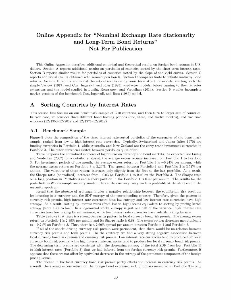
Online Appendix for “Nominal Exchange Rate Stationarityand Long-Term Bond Returns”

—Not For Publication—

This Online Appendix describes additional empirical and theoretical results on foreign bond returns in U.S.dollars. Section A reports additional results on portfolios of countries sorted by the short-term interest rates.Section B reports similar results for portfolios of countries sorted by the slope of the yield curves. Section Creports additional results obtained with zero-coupon bonds. Section D compares finite to infinite maturity bondreturns. Section E reports additional theoretical results on dynamic term structure models, starting with thesimple Vasicek (1977) and Cox, Ingersoll, and Ross (1985) one-factor models, before turning to their k-factorextensions and the model studied in Lustig, Roussanov, and Verdelhan (2014). Section F studies incompletemarket versions of the benchmark Cox, Ingersoll, and Ross (1985) model.

A Sorting Countries by Interest Rates

This section first focuses on our benchmark sample of G10 countries, and then turn to larger sets of countries.In each case, we consider three different bond holding periods (one, three, and twelve months), and two timewindows (12/1950–12/2012 and 12/1971–12/2012).

A.1 Benchmark Sample

Figure 5 plots the composition of the three interest rate-sorted portfolios of the currencies of the benchmarksample, ranked from low to high interest rate currencies. Typically, Switzerland and Japan (after 1970) arefunding currencies in Portfolio 1, while Australia and New Zealand are the carry trade investment currencies inPortfolio 3. The other currencies switch between portfolios quite often.

Table 3 reports the annualized moments of log returns on currency and bond markets. As expected [see Lustigand Verdelhan (2007) for a detailed analysis], the average excess returns increase from Portfolio 1 to Portfolio3. For investment periods of one month, the average excess return on Portfolio 1 is −0.24% per annum, whilethe average excess return on Portfolio 3 is 3.26%. The spread between Portfolio 1 and Portfolio 3 is 3.51% perannum. The volatility of these returns increases only slightly from the first to the last portfolio. As a result,the Sharpe ratio (annualized) increases from −0.03 on Portfolio 1 to 0.40 on the Portfolio 3. The Sharpe ratioon a long position in Portfolio 3 and a short position in the Portfolio 1 is 0.49 per annum. The results for thepost-Bretton-Woods sample are very similar. Hence, the currency carry trade is profitable at the short end of thematurity spectrum.

Recall that the absence of arbitrage implies a negative relationship between the equilibrium risk premiumfor investing in a currency and the SDF entropy of the corresponding country. Therefore, given the pattern incurrency risk premia, high interest rate currencies have low entropy and low interest rate currencies have highentropy. As a result, sorting by interest rates (from low to high) seems equivalent to sorting by pricing kernelentropy (from high to low). In a log-normal world, entropy is just one half of the variance: high interest ratecurrencies have low pricing kernel variance, while low interest rate currencies have volatile pricing kernels.

Table 3 shows that there is a strong decreasing pattern in local currency bond risk premia. The average excessreturn on Portfolio 1 is 2.39% per annum and its Sharpe ratio is 0.68. The excess return decreases monotonicallyto −0.21% on Portfolio 3. Thus, there is a 2.60% spread per annum between Portfolio 1 and Portfolio 3.

If all of the shocks driving currency risk premia were permanent, then there would be no relation betweencurrency risk premia and term premia. To the contrary, we find a very strong negative association betweenlocal currency bond risk premia and currency risk premia. Low interest rate currencies tend to produce high localcurrency bond risk premia, while high interest rate currencies tend to produce low local currency bond risk premia.The decreasing term premia are consistent with the decreasing entropy of the total SDF from low (Portfolio 1)to high interest rates (Portfolio 3) that we had inferred from the foreign currency risk premia. Furthermore, itappears that these are not offset by equivalent decreases in the entropy of the permanent component of the foreignpricing kernel.

The decline in the local currency bond risk premia partly offsets the increase in currency risk premia. Asa result, the average excess return on the foreign bond expressed in U.S. dollars measured in Portfolio 3 is only

50

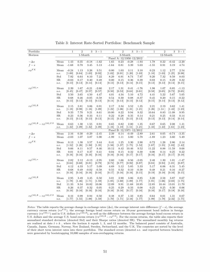
Table 3: Interest Rate-Sorted Portfolios: Benchmark Sample

Portfolio 1 2 3 3− 1 1 2 3 3− 1 1 2 3 3− 1

Horizon 1-Month 3-Month 12-MonthPanel A: 12/1950–12/2012

−∆s Mean 1.43 0.35 -0.18 -1.62 1.65 0.23 -0.28 -1.93 1.78 0.22 -0.42 -2.20f − s Mean -1.68 0.78 3.45 5.13 -1.64 0.81 3.39 5.03 -1.55 0.91 3.19 4.74

rxFX Mean -0.24 1.13 3.26 3.51 0.00 1.03 3.11 3.10 0.23 1.12 2.77 2.54s.e. [1.00] [0.84] [1.03] [0.92] [1.02] [0.91] [1.20] [1.03] [1.10] [1.03] [1.25] [0.98]Std 7.92 6.64 8.10 7.22 8.29 6.91 8.74 7.97 9.20 7.32 9.59 8.03SR -0.03 0.17 0.40 0.49 0.00 0.15 0.36 0.39 0.03 0.15 0.29 0.32s.e. [0.13] [0.13] [0.14] [0.14] [0.13] [0.13] [0.14] [0.15] [0.13] [0.13] [0.14] [0.15]

rx(10),∗ Mean 2.39 1.67 -0.21 -2.60 2.17 1.31 0.41 -1.76 1.98 1.07 0.85 -1.13s.e. [0.45] [0.47] [0.57] [0.57] [0.50] [0.53] [0.64] [0.61] [0.58] [0.65] [0.72] [0.65]Std 3.50 3.65 4.50 4.47 4.01 4.34 5.10 4.72 4.41 5.22 5.67 5.05SR 0.68 0.46 -0.05 -0.58 0.54 0.30 0.08 -0.37 0.45 0.20 0.15 -0.22s.e. [0.13] [0.13] [0.13] [0.13] [0.14] [0.13] [0.13] [0.12] [0.15] [0.14] [0.13] [0.12]

rx(10),$ Mean 2.15 2.81 3.06 0.91 2.17 2.34 3.52 1.35 2.21 2.19 3.62 1.41s.e. [1.18] [0.98] [1.16] [1.09] [1.22] [1.06] [1.31] [1.21] [1.26] [1.14 ] [1.42] [1.23]Std 9.33 7.70 9.21 8.61 10.00 8.22 9.94 9.32 10.64 8.83 11.08 9.95SR 0.23 0.36 0.33 0.11 0.22 0.28 0.35 0.14 0.21 0.25 0.33 0.14s.e. [0.13] [0.13] [0.13] [0.13] [0.13] [0.13] [0.13] [0.13] [0.13] [0.13] [0.14] [0.14]

rx(10),$ − rx(10),US Mean 0.63 1.30 1.55 0.91 0.65 0.82 2.00 1.35 0.67 0.65 2.08 1.41s.e. [1.22] [1.09] [1.32] [1.09] [1.16] [1.18] [1.51] [1.21] [1.33] [1.22] [1.61] [1.23]

Panel B: 12/1971–12/2012−∆s Mean 2.16 0.30 -0.29 -2.45 2.39 0.14 -0.49 -2.89 2.61 0.05 -0.74 -3.35f − s Mean -2.03 1.07 3.87 5.90 -1.99 1.11 3.80 5.78 -1.89 1.23 3.60 5.49

rxFX Mean 0.13 1.38 3.57 3.44 0.41 1.25 3.30 2.90 0.72 1.28 2.86 2.14s.e. [1.52] [1.26] [1.50] [1.35] [1.56] [1.37] [1.75] [1.52] [1.67] [1.55] [1.82] [1.42]Std 9.66 8.11 9.57 8.46 10.12 8.42 10.46 9.52 11.22 8.88 11.59 9.68SR 0.01 0.17 0.37 0.41 0.04 0.15 0.32 0.30 0.06 0.14 0.25 0.22s.e. [0.16] [0.16] [0.16] [0.16] [0.16] [0.16] [0.17] [0.17] [0.16] [0.17] [0.17] [0.18]

rx(10),∗ Mean 2.82 2.12 -0.13 -2.95 2.60 1.66 0.56 -2.05 2.48 1.30 1.01 -1.47s.e. [0.64] [0.68] [0.81] [0.79] [0.72] [0.77] [0.92] [0.87] [0.84] [0.94] [1.01] [0.87]Std 4.12 4.33 5.17 5.09 4.69 5.12 5.85 5.33 5.17 6.06 6.31 5.45SR 0.68 0.49 -0.02 -0.58 0.55 0.32 0.10 -0.38 0.48 0.21 0.16 -0.27s.e. [0.16] [0.16] [0.16] [0.16] [0.17] [0.16] [0.16] [0.15] [0.19] [0.18] [0.16] [0.15]

rx(10),$ Mean 2.95 3.49 3.45 0.50 3.01 2.90 3.86 0.85 3.20 2.58 3.87 0.67s.e. [1.78] [1.46] [1.71] [1.59] [1.85] [1.60] [1.89] [1.77] [1.91] [1.66] [2.03] [1.75]Std 11.33 9.34 10.82 10.06 12.09 9.91 11.68 10.95 12.85 10.44 13.01 11.70SR 0.26 0.37 0.32 0.05 0.25 0.29 0.33 0.08 0.25 0.25 0.30 0.06s.e. [0.16] [0.16] [0.16] [0.16] [0.16] [0.16] [0.17] [0.16] [0.16] [0.17] [0.18] [0.16]

rx(10),$ − rx(10),US Mean 0.44 0.99 0.94 0.50 0.48 0.37 1.33 0.85 0.64 0.01 1.31 0.67s.e. [1.77] [1.55] [1.88] [1.59] [1.70] [1.71] [2.16] [1.77] [1.99] [1.78] [2.32] [1.75]

Notes: The table reports the average change in exchange rates (∆s), the average interest rate difference (f −s), the averagecurrency excess return (rxFX), the average foreign bond excess return on 10-year government bond indices in foreigncurrency (rx(10),∗) and in U.S. dollars (rx(10),$), as well as the difference between the average foreign bond excess return inU.S. dollars and the average U.S. bond excess return (rx(10),$ − rxUS). For the excess returns, the table also reports theirannualized standard deviation (denoted Std) and their Sharpe ratios (denoted SR). The annualized monthly log returnsare realized at date t + k , where the horizon k equals 1, 3, and 12 months. The balanced panel consists of Australia,Canada, Japan, Germany, Norway, New Zealand, Sweden, Switzerland, and the U.K. The countries are sorted by the levelof their short term interest rates into three portfolios. The standard errors (denoted s.e. and reported between brackets)were generated by bootstrapping 10,000 samples of non-overlapping returns.

51

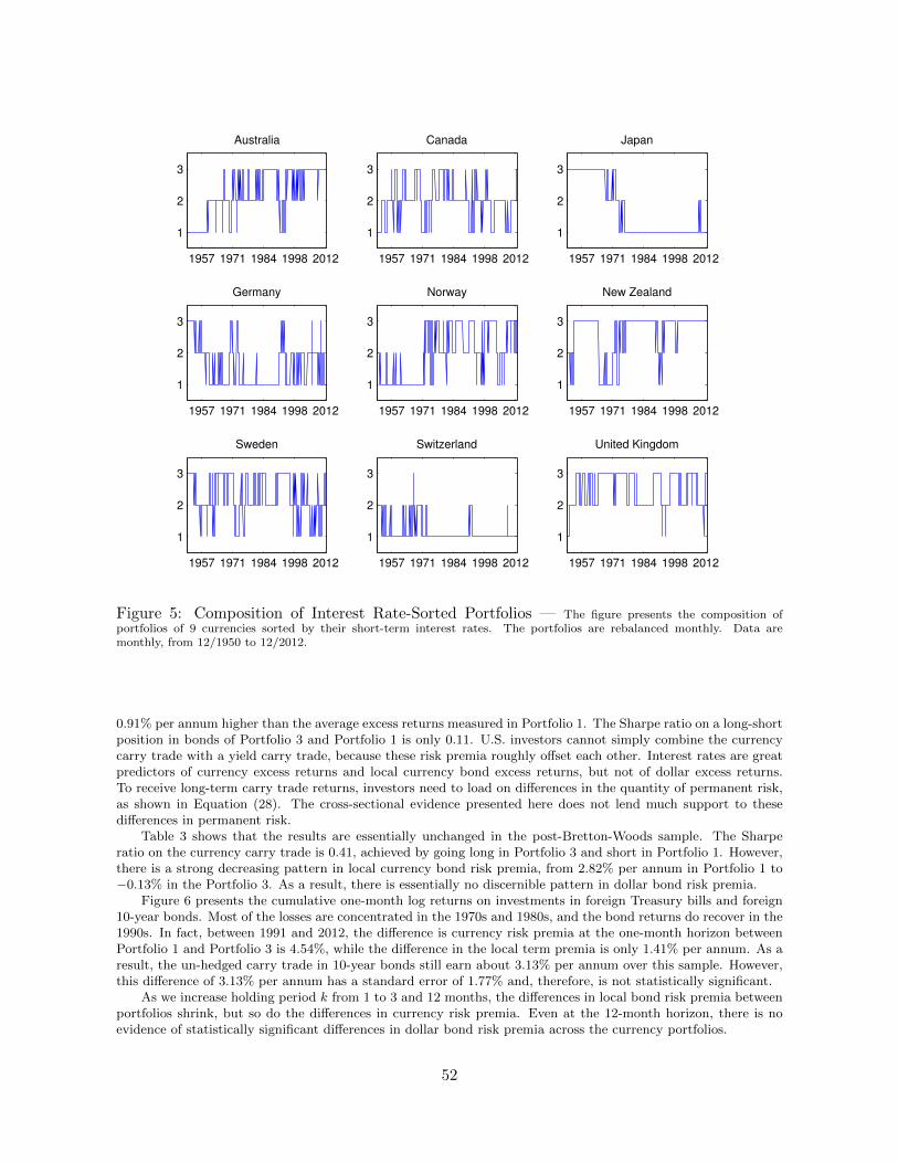
1957 1971 1984 1998 2012

1

2

3

Australia

1957 1971 1984 1998 2012

1

2

3

Canada

1957 1971 1984 1998 2012

1

2

3

Japan

1957 1971 1984 1998 2012

1

2

3

Germany

1957 1971 1984 1998 2012

1

2

3

Norway

1957 1971 1984 1998 2012

1

2

3

New Zealand

1957 1971 1984 1998 2012

1

2

3

Sweden

1957 1971 1984 1998 2012

1

2

3

Switzerland

1957 1971 1984 1998 2012

1

2

3

United Kingdom

Figure 5: Composition of Interest Rate-Sorted Portfolios — The figure presents the composition ofportfolios of 9 currencies sorted by their short-term interest rates. The portfolios are rebalanced monthly. Data aremonthly, from 12/1950 to 12/2012.

0.91% per annum higher than the average excess returns measured in Portfolio 1. The Sharpe ratio on a long-shortposition in bonds of Portfolio 3 and Portfolio 1 is only 0.11. U.S. investors cannot simply combine the currencycarry trade with a yield carry trade, because these risk premia roughly offset each other. Interest rates are greatpredictors of currency excess returns and local currency bond excess returns, but not of dollar excess returns.To receive long-term carry trade returns, investors need to load on differences in the quantity of permanent risk,as shown in Equation (28). The cross-sectional evidence presented here does not lend much support to thesedifferences in permanent risk.

Table 3 shows that the results are essentially unchanged in the post-Bretton-Woods sample. The Sharperatio on the currency carry trade is 0.41, achieved by going long in Portfolio 3 and short in Portfolio 1. However,there is a strong decreasing pattern in local currency bond risk premia, from 2.82% per annum in Portfolio 1 to−0.13% in the Portfolio 3. As a result, there is essentially no discernible pattern in dollar bond risk premia.

Figure 6 presents the cumulative one-month log returns on investments in foreign Treasury bills and foreign10-year bonds. Most of the losses are concentrated in the 1970s and 1980s, and the bond returns do recover in the1990s. In fact, between 1991 and 2012, the difference is currency risk premia at the one-month horizon betweenPortfolio 1 and Portfolio 3 is 4.54%, while the difference in the local term premia is only 1.41% per annum. As aresult, the un-hedged carry trade in 10-year bonds still earn about 3.13% per annum over this sample. However,this difference of 3.13% per annum has a standard error of 1.77% and, therefore, is not statistically significant.

As we increase holding period k from 1 to 3 and 12 months, the differences in local bond risk premia betweenportfolios shrink, but so do the differences in currency risk premia. Even at the 12-month horizon, there is noevidence of statistically significant differences in dollar bond risk premia across the currency portfolios.

52

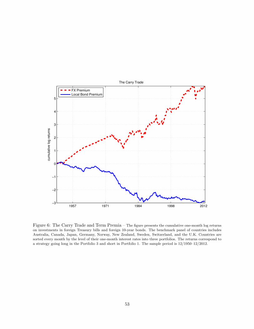
1957 1971 1984 1998 2012−3

−2

−1

0

1

2

3

4

5

The Carry Trade

cum

ula

tive log r

etu

rns

FX Premium

Local Bond Premium

Figure 6: The Carry Trade and Term Premia – The figure presents the cumulative one-month log returnson investments in foreign Treasury bills and foreign 10-year bonds. The benchmark panel of countries includesAustralia, Canada, Japan, Germany, Norway, New Zealand, Sweden, Switzerland, and the U.K. Countries aresorted every month by the level of their one-month interest rates into three portfolios. The returns correspond toa strategy going long in the Portfolio 3 and short in Portfolio 1. The sample period is 12/1950–12/2012.

53

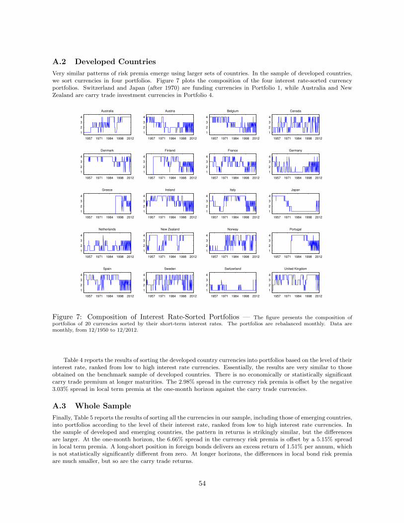
A.2 Developed Countries

Very similar patterns of risk premia emerge using larger sets of countries. In the sample of developed countries,we sort currencies in four portfolios. Figure 7 plots the composition of the four interest rate-sorted currencyportfolios. Switzerland and Japan (after 1970) are funding currencies in Portfolio 1, while Australia and NewZealand are carry trade investment currencies in Portfolio 4.

1957 1971 1984 1998 2012

1

2

3

4

Australia

1957 1971 1984 1998 2012

1

2

3

4

Austria

1957 1971 1984 1998 2012

1

2

3

4

Belgium

1957 1971 1984 1998 2012

1

2

3

4

Canada

1957 1971 1984 1998 2012

1

2

3

4

Denmark

1957 1971 1984 1998 2012

1

2

3

4

Finland

1957 1971 1984 1998 2012

1

2

3

4

France

1957 1971 1984 1998 2012

1

2

3

4

Germany

1957 1971 1984 1998 2012

1

2

3

4

Greece

1957 1971 1984 1998 2012

1

2

3

4

Ireland

1957 1971 1984 1998 2012

1

2

3

4

Italy

1957 1971 1984 1998 2012

1

2

3

4

Japan

1957 1971 1984 1998 2012

1

2

3

4

Netherlands

1957 1971 1984 1998 2012

1

2

3

4

New Zealand

1957 1971 1984 1998 2012

1

2

3

4

Norway

1957 1971 1984 1998 2012

1

2

3

4

Portugal

1957 1971 1984 1998 2012

1

2

3

4

Spain

1957 1971 1984 1998 2012

1

2

3

4

Sweden

1957 1971 1984 1998 2012

1

2

3

4

Switzerland

1957 1971 1984 1998 2012

1

2

3

4

United Kingdom

Figure 7: Composition of Interest Rate-Sorted Portfolios — The figure presents the composition ofportfolios of 20 currencies sorted by their short-term interest rates. The portfolios are rebalanced monthly. Data aremonthly, from 12/1950 to 12/2012.

Table 4 reports the results of sorting the developed country currencies into portfolios based on the level of theirinterest rate, ranked from low to high interest rate currencies. Essentially, the results are very similar to thoseobtained on the benchmark sample of developed countries. There is no economically or statistically significantcarry trade premium at longer maturities. The 2.98% spread in the currency risk premia is offset by the negative3.03% spread in local term premia at the one-month horizon against the carry trade currencies.

A.3 Whole Sample

Finally, Table 5 reports the results of sorting all the currencies in our sample, including those of emerging countries,into portfolios according to the level of their interest rate, ranked from low to high interest rate currencies. Inthe sample of developed and emerging countries, the pattern in returns is strikingly similar, but the differencesare larger. At the one-month horizon, the 6.66% spread in the currency risk premia is offset by a 5.15% spreadin local term premia. A long-short position in foreign bonds delivers an excess return of 1.51% per annum, whichis not statistically significantly different from zero. At longer horizons, the differences in local bond risk premiaare much smaller, but so are the carry trade returns.

54

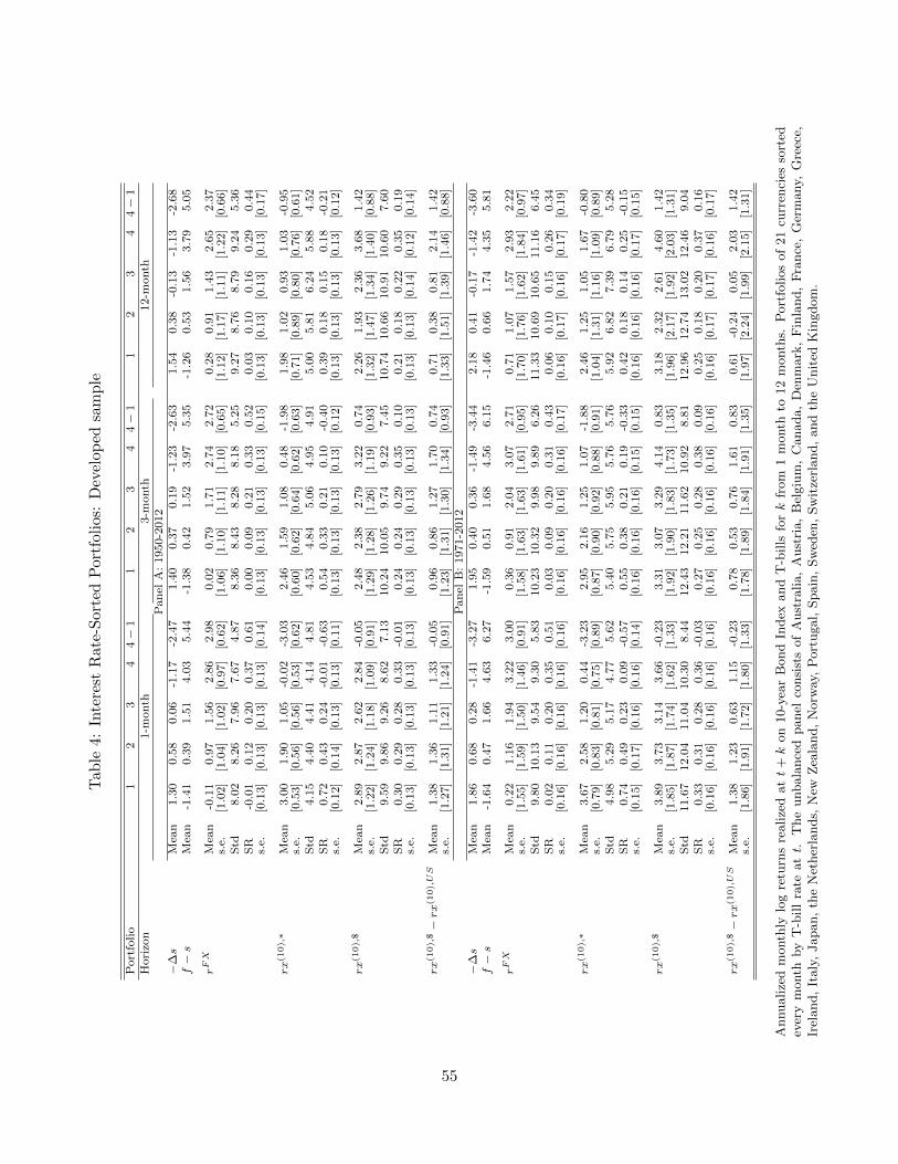
Tab

le4:

Inte

rest

Rat

e-S

orte

dP

ortf

olio

s:D

evel

oped

sam

ple

Port

folio

12

34

4−

11

23

44−

11

23

44−

1H

ori

zon

1-m

onth

3-m

onth

12-m

onth

Pan

elA

:1950-2

012

−∆s

Mea

n1.3

00.5

80.0

6-1

.17

-2.4

71.4

00.3

70.1

9-1

.23

-2.6

31.5

40.3

8-0

.13

-1.1

3-2

.68

f−s

Mea

n-1

.41

0.3

91.5

14.0

35.4

4-1

.38

0.4

21.5

23.9

75.3

5-1

.26

0.5

31.5

63.7

95.0

5

rFX

Mea

n-0

.11

0.9

71.5

62.8

62.9

80.0

20.7

91.7

12.7

42.7

20.2

80.9

11.4

32.6

52.3

7s.

e.[1

.02]

[1.0

4]

[1.0

2]

[0.9

7]

[0.6

2]

[1.0

6]

[1.1

0]

[1.1

1]

[1.1

0]

[0.6

5]

[1.1

2]

[1.1

7]

[1.1

1]

[1.2

2]

[0.6

6]

Std

8.0

28.2

67.9

67.6

74.8

78.3

68.4

38.2

88.1

85.2

59.2

78.7

68.7

99.2

45.3

6S

R-0

.01

0.1

20.2

00.3

70.6

10.0

00.0

90.2

10.3

30.5

20.0

30.1

00.1

60.2

90.4

4s.

e.[0

.13]

[0.1

3]

[0.1

3]

[0.1

3]

[0.1

4]

[0.1

3]

[0.1

3]

[0.1

3]

[0.1

3]

[0.1

5]

[0.1

3]

[0.1

3]

[0.1

3]

[0.1

3]

[0.1

7]

rx

(10),∗

Mea

n3.0

01.9

01.0

5-0

.02

-3.0

32.4

61.5

91.0

80.4

8-1

.98

1.9

81.0

20.9

31.0

3-0

.95

s.e.

[0.5

3]

[0.5

6]

[0.5

6]

[0.5

3]

[0.6

2]

[0.6

0]

[0.6

2]

[0.6

4]

[0.6

2]

[0.6

3]

[0.7

1]

[0.8

9]

[0.8

0]

[0.7

6]

[0.6

1]

Std

4.1

54.4

04.4

14.1

44.8

14.5

34.8

45.0

64.9

54.9

15.0

05.8

16.2

45.8

84.5

2S

R0.7

20.4

30.2

4-0

.01

-0.6

30.5

40.3

30.2

10.1

0-0

.40

0.3

90.1

80.1

50.1

8-0

.21

s.e.

[0.1

2]

[0.1

4]

[0.1

3]

[0.1

3]

[0.1

1]

[0.1

3]

[0.1

3]

[0.1

3]

[0.1

3]

[0.1

2]

[0.1

3]

[0.1

3]

[0.1

3]

[0.1

3]

[0.1

2]

rx

(10),

$M

ean

2.8

92.8

72.6

22.8

4-0

.05

2.4

82.3

82.7

93.2

20.7

42.2

61.9

32.3

63.6

81.4

2s.

e.[1

.22]

[1.2

4]

[1.1

8]

[1.0

9]

[0.9

1]

[1.2

9]

[1.2

8]

[1.2

6]

[1.1

9]

[0.9

3]

[1.3

2]

[1.4

7]

[1.3

4]

[1.4

0]

[0.8

8]

Std

9.5

99.8

69.2

68.6

27.1

310.2

410.0

59.7

49.2

27.4

510.7

410.6

610.9

110.6

07.6

0S

R0.3

00.2

90.2

80.3

3-0

.01

0.2

40.2

40.2

90.3

50.1

00.2

10.1

80.2

20.3

50.1

9s.

e.[0

.13]

[0.1

3]

[0.1

3]

[0.1

3]

[0.1

3]

[0.1

3]

[0.1

3]

[0.1

3]

[0.1

3]

[0.1

3]

[0.1

3]

[0.1

3]

[0.1

4]

[0.1

2]

[0.1

4]

rx

(10),

$−rx

(10),US

Mea

n1.3

81.3

61.1

11.3

3-0

.05

0.9

60.8

61.2

71.7

00.7

40.7

10.3

80.8

12.1

41.4

2s.

e.[1

.27]

[1.3

1]

[1.2

1]

[1.2

4]

[0.9

1]

[1.2

3]

[1.3

1]

[1.3

0]

[1.3

4]

[0.9

3]

[1.3

3]

[1.5

1]

[1.3

9]

[1.4

6]

[0.8

8]

Pan

elB

:1971-2

012

−∆s

Mea

n1.8

60.6

80.2

8-1

.41

-3.2

71.9

50.4

00.3

6-1

.49

-3.4

42.1

80.4

1-0

.17

-1.4

2-3

.60

f−s

Mea

n-1

.64

0.4

71.6

64.6

36.2

7-1

.59

0.5

11.6

84.5

66.1

5-1

.46

0.6

61.7

44.3

55.8

1

rFX

Mea

n0.2

21.1

61.9

43.2

23.0

00.3

60.9

12.0

43.0

72.7

10.7

11.0

71.5

72.9

32.2

2s.

e.[1

.55]

[1.5

9]

[1.5

0]

[1.4

6]

[0.9

1]

[1.5

8]

[1.6

3]

[1.6

3]

[1.6

1]

[0.9

5]

[1.7

0]

[1.7

6]

[1.6

2]

[1.8

4]

[0.9

7]

Std

9.8

010.1

39.5

49.3

05.8

310.2

310.3

29.9

89.8

96.2

611.3

310.6

910.6

511.1

66.4

5S

R0.0

20.1

10.2

00.3

50.5

10.0

30.0

90.2

00.3

10.4

30.0

60.1

00.1

50.2

60.3

4s.

e.[0

.16]

[0.1

6]

[0.1

6]

[0.1

6]

[0.1

6]

[0.1

6]

[0.1

6]

[0.1

6]

[0.1

6]

[0.1

7]

[0.1

6]

[0.1

7]

[0.1

6]

[0.1

7]

[0.1

9]

rx

(10),∗

Mea

n3.6

72.5

81.2

00.4

4-3

.23

2.9

52.1

61.2

51.0

7-1

.88

2.4

61.2

51.0

51.6

7-0

.80

s.e.

[0.7

9]

[0.8

3]

[0.8

1]

[0.7

5]

[0.8

9]

[0.8

7]

[0.9

0]

[0.9

2]

[0.8

8]

[0.9

1]

[1.0

4]

[1.3

1]

[1.1

6]

[1.0

9]

[0.8

9]

Std

4.9

85.2

95.1

74.7

75.6

25.4

05.7

55.9

55.7

65.7

65.9

26.8

27.3

96.7

95.2

8S

R0.7

40.4

90.2

30.0

9-0

.57

0.5

50.3

80.2

10.1

9-0

.33

0.4

20.1

80.1

40.2

5-0

.15

s.e.

[0.1

5]

[0.1

7]

[0.1

6]

[0.1

6]

[0.1

4]

[0.1

6]

[0.1

6]

[0.1

6]

[0.1

5]

[0.1

5]

[0.1

6]

[0.1

6]

[0.1

6]

[0.1

7]

[0.1

5]

rx

(10),

$M

ean

3.8

93.7

33.1

43.6

6-0

.23

3.3

13.0

73.2

94.1

40.8

33.1

82.3

22.6

14.6

01.4

2s.

e.[1

.85]

[1.8

7]

[1.7

4]

[1.6

2]

[1.3

3]

[1.9

2]

[1.9

0]

[1.8

3]

[1.7

3]

[1.3

5]

[1.9

6]

[2.1

7]

[1.9

2]

[2.0

3]

[1.3

1]

Std

11.6

712.0

411.0

410.3

08.4

412.4

312.2

111.6

210.9

28.8

112.9

612.7

413.0

212.4

69.0

4S

R0.3

30.3

10.2

80.3

6-0

.03

0.2

70.2

50.2

80.3

80.0

90.2

50.1

80.2

00.3

70.1

6s.

e.[0

.16]

[0.1

6]

[0.1

6]

[0.1

6]

[0.1

6]

[0.1

6]

[0.1

6]

[0.1

6]

[0.1

6]

[0.1

6]

[0.1

6]

[0.1

7]

[0.1

7]

[0.1

6]

[0.1

7]

rx

(10),

$−rx

(10),US

Mea

n1.3

81.2

30.6

31.1

5-0

.23

0.7

80.5

30.7

61.6

10.8

30.6

1-0

.24

0.0

52.0

31.4

2s.

e.[1

.86]

[1.9

1]

[1.7

2]

[1.8

0]

[1.3

3]

[1.7

8]

[1.8

9]

[1.8

4]

[1.9

1]

[1.3

5]

[1.9

7]

[2.2

4]

[1.9

9]

[2.1

5]

[1.3

1]

Annualize

dm

onth

lylo

gre

turn

sre

alize

datt

+k

on

10-y

ear

Bond

Index

and

T-b

ills

fork

from

1m

onth

to12

month

s.P

ort

folios

of

21

curr

enci

esso

rted

ever

ym

onth

by

T-b

ill

rate

att.

The

unbala

nce

dpanel

consi

sts

of

Aust

ralia,

Aust

ria,

Bel

giu

m,

Canada,

Den

mark

,F

inla

nd,

Fra

nce

,G

erm

any,

Gre

ece,

Irel

and,

Italy

,Japan,

the

Net

her

lands,

New

Zea

land,

Norw

ay,

Port

ugal,

Spain

,Sw

eden

,Sw

itze

rland,

and

the

Unit

edK

ingdom

.

55

As in the previous samples, the rate at which the high interest rate currencies depreciate (2.99% per annum)is not high enough to offset the interest rate difference of 6.55%. Similarly, the rate at which the low interestrate currencies appreciate (0.43% per annum) is not high enough to offset the low interest rates (3.52% lowerthan the U.S. interest rate). Uncovered interest rate parity fails in the cross-section. However, the bond returndifferences (in local currency) are closer to being offset by the rate of depreciation. The bond return spread is4.63% per annum for the last portfolio, compared to an annual depreciation rate of 6.55%, while the spread onthe first portfolio is −0.29%, compared to depreciation of −0.43%.

B Sorting Currencies by the Slope of the Yield Curve

This section presents additional evidence on slope-sorted portfolios, again considering first our benchmark sampleof G10 countries before turning to larger sets of developed and emerging countries.

In the sample of developed countries, the steep-slope (low yielding) currencies are typically countries likeGermany, the Netherlands, Japan, and Switzerland, while the flat-slope (high-yielding) currencies are typicallyAustralia, New Zealand, Denmark and the U.K.

At the one-month horizon, the 2.4% spread in currency excess returns obtained in this sample is more thanoffset by the 5.9% spread in local term premia. This produces a statistically significant 3.5% return on a positionthat is long in the low yielding, high slope currencies and short in the high yielding, low slope currencies. Theseresults are essentially unchanged in the post-Bretton-Woods sample. At longer horizons, the currency excessreturns and the local risk premia almost fully offset each other.

In the entire sample of countries, including the emerging market countries, the difference in currency riskpremia at the one-month horizon is 3.04% per annum, which is more than offset by a 8.37% difference in localterm premia. As a result, investors earn 5.33% per annum on a long-short position in foreign bond portfoliosof slope-sorted currencies. As before, this involves shorting the flat-yield-curve currencies, typically high interestrate currencies, and going long in the steep-slope currencies, typically the low interest rate ones. The annualizedSharpe ratio on this long-short strategy is 0.60.

B.1 Benchmark Sample

Figure 8 presents the composition over time of portfolios of the 9 currencies of the benchmark sample sorted bythe slope of the yield curve.

Consistent with this distribution of interest rates, average currency excess returns decrease across portfolios.Table 6 reports the annualized moments of log returns on the three slope-sorted portfolios. Average currencyexcess returns decline from 3.0% per annum on Portfolio 1 to 0.5% per annum on the Portfolio 3 over the last 60years. Therefore, a long-short position of investing in steep-yield-curve currencies and shorting flat-yield-curvecurrencies delivers a currency excess return of −2.5% per annum and a Sharpe ratio of −0.4. Our findings confirmthose of Ang and Chen (2010). The slope of the yield curve predicts currency excess returns very well. However,note that this result is not mechanical; the spread in the slopes (reported on the third line) is much smaller thanthe spread in excess returns. Deviations from long-term U.I.P are again small and by construction impreciselyestimated.

Turning to the holding period returns on local bonds, average bond excess returns increase across portfolios.Portfolio 1 produces negative bond excess returns of −0.9% per annum, compared to 3.3% per annum on Portfolio3. Importantly, this strategy involves long positions in bonds issued by countries like Germany and Japan. Theseare countries with fairly liquid bond markets and low sovereign credit risk. As a result, credit and liquidity riskdifferences are unlikely candidate explanations for the return differences. Here again, the bond and currencyexcess returns move in opposite directions across portfolios.

Turing to the returns on foreign bonds in U.S. dollars, we do not obtain significant differences across portfolios.Average bond excess returns in U.S. dollars tend to increase from the first (flat-yield-curve) portfolio to the last(steep-yield-curve), but a long-short strategy does not deliver a significant excess return. Local bond and currencyrisk premier offset each other. We get similar findings when we restrict our analysis to the post-Bretton Woodssample.

As a robustness check, Table 7 reports the results of sorting on the yield curve slope on the benchmark G10sample using different holding periods (one, three, and 12 months).

56

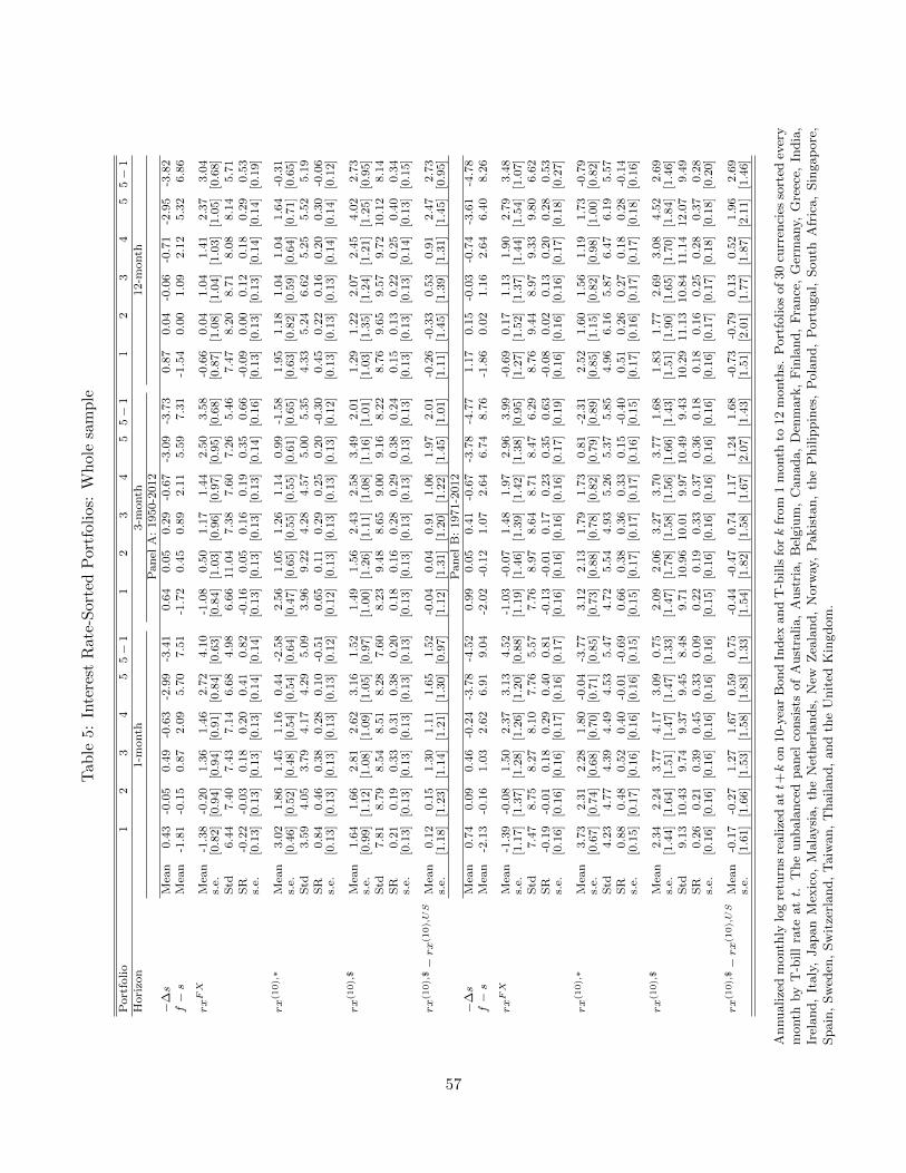
Tab

le5:

Inte

rest

Rat

e-S

orte

dP

ortf

olio

s:W

hol

esa

mp

le

Port

folio

12

34

55−

11

23

45

5−

11

23

45

5−

1H

ori

zon

1-m

onth

3-m

onth

12-m

onth

Pan

elA

:1950-2

012

−∆s

Mea

n0.4

3-0

.05

0.4

9-0

.63

-2.9

9-3

.41

0.6

40.0

50.2

9-0

.67

-3.0

9-3

.73

0.8

70.0

4-0

.06

-0.7

1-2

.95

-3.8

2f−s

Mea

n-1

.81

-0.1

50.8

72.0

95.7

07.5

1-1

.72

0.4

50.8

92.1

15.5

97.3

1-1

.54

0.0

01.0

92.1

25.3

26.8

6

rxFX

Mea

n-1

.38

-0.2

01.3

61.4

62.7

24.1

0-1

.08

0.5

01.1

71.4

42.5

03.5

8-0

.66

0.0

41.0

41.4

12.3

73.0

4s.

e.[0

.82]

[0.9

4]

[0.9

4]

[0.9

1]

[0.8

4]

[0.6

3]

[0.8

4]

[1.0

3]

[0.9

6]

[0.9

7]

[0.9

5]

[0.6

8]

[0.8

7]

[1.0

8]

[1.0

4]

[1.0

3]

[1.0

5]

[0.6

8]

Std

6.4

47.4

07.4

37.1

46.6

84.9

86.6

611.0

47.3

87.6

07.2

65.4

67.4

78.2

08.7

18.0

88.1

45.7

1S

R-0

.22

-0.0

30.1

80.2

00.4

10.8

2-0

.16

0.0

50.1

60.1

90.3

50.6

6-0

.09

0.0

00.1

20.1

80.2

90.5

3s.

e.[0

.13]

[0.1

3]

[0.1

3]

[0.1

3]

[0.1

4]

[0.1

4]

[0.1

3]

[0.1

3]

[0.1

3]

[0.1

3]

[0.1

4]

[0.1

6]

[0.1

3]

[0.1

3]

[0.1

3]

[0.1

4]

[0.1

4]

[0.1

9]

rx

(10),∗

Mea

n3.0

21.8

61.4

51.1

60.4

4-2

.58

2.5

61.0

51.2

61.1

40.9

9-1

.58

1.9

51.1

81.0

41.0

41.6

4-0

.31

s.e.

[0.4

6]

[0.5

2]

[0.4

8]

[0.5

4]

[0.5

4]

[0.6

4]

[0.4

7]

[0.6

5]

[0.5

5]

[0.5

5]

[0.6

1]

[0.6

5]

[0.6

3]

[0.8

2]

[0.5

9]

[0.6

4]

[0.7

1]

[0.6

5]

Std

3.5

94.0

53.7

94.1

74.2

95.0

93.9

69.2

24.2

84.5

75.0

05.3

54.3

35.2

46.6

25.2

55.5

25.1

9S

R0.8

40.4

60.3

80.2

80.1

0-0

.51

0.6

50.1

10.2

90.2

50.2

0-0

.30

0.4

50.2

20.1

60.2

00.3

0-0

.06

s.e.

[0.1

3]

[0.1

3]

[0.1

3]

[0.1

3]

[0.1

3]

[0.1

2]

[0.1

2]

[0.1

3]

[0.1

3]

[0.1

3]

[0.1

3]

[0.1

2]

[0.1

3]

[0.1

3]

[0.1

3]

[0.1

4]

[0.1

4]

[0.1

2]

rx

(10),

$M

ean

1.6

41.6

62.8

12.6

23.1

61.5

21.4

91.5

62.4

32.5

83.4

92.0

11.2

91.2

22.0

72.4

54.0

22.7

3s.

e.[0

.99]

[1.1

2]

[1.0

8]

[1.0

9]

[1.0

5]

[0.9

7]

[1.0

0]

[1.2

6]

[1.1

1]

[1.0

8]

[1.1

6]

[1.0

1]

[1.0

3]

[1.3

5]

[1.2

4]

[1.2

1]

[1.2

5]

[0.9

5]

Std

7.8

18.7

98.5

48.5

18.2

87.6

08.2

39.4

88.6

59.0

09.1

68.2

28.7

69.6

59.5

79.7

210.1

28.1

4S

R0.2

10.1

90.3

30.3

10.3

80.2

00.1

80.1

60.2

80.2

90.3

80.2

40.1

50.1

30.2

20.2

50.4

00.3

4s.

e.[0

.13]

[0.1

3]

[0.1

3]

[0.1

3]

[0.1

3]

[0.1

3]

[0.1

3]

[0.1

3]

[0.1

3]

[0.1

3]

[0.1

3]

[0.1

3]

[0.1

3]

[0.1

3]

[0.1

3]

[0.1

4]

[0.1

3]

[0.1

5]

rx

(10),

$−rx

(10),US

Mea

n0.1

20.1

51.3

01.1

11.6

51.5

2-0

.04

0.0

40.9

11.0

61.9

72.0

1-0

.26

-0.3

30.5

30.9

12.4

72.7

3s.

e.[1

.18]

[1.2

3]

[1.1

4]

[1.2

1]

[1.3

0]

[0.9

7]

[1.1

2]

[1.3

1]

[1.2

0]

[1.2

2]

[1.4

5]

[1.0

1]

[1.1

1]

[1.4

5]

[1.3

9]

[1.3

1]

[1.4

5]

[0.9

5]

Pan

elB

:1971-2

012

−∆s

Mea

n0.7

40.0

90.4

6-0

.24

-3.7

8-4

.52

0.9

90.0

50.4

1-0

.67

-3.7

8-4

.77

1.1

70.1

5-0

.03

-0.7

4-3

.61

-4.7

8f−s

Mea

n-2

.13

-0.1

61.0

32.6

26.9

19.0

4-2

.02

-0.1

21.0

72.6

46.7

48.7

6-1

.86

0.0

21.1

62.6

46.4

08.2

6

rxFX

Mea

n-1

.39

-0.0

81.5

02.3

73.1

34.5

2-1

.03

-0.0

71.4

81.9

72.9

63.9

9-0

.69

0.1

71.1

31.9

02.7

93.4

8s.

e.[1

.17]

[1.3

7]

[1.2

8]

[1.2

6]

[1.2

0]

[0.8

8]

[1.1

9]

[1.4

6]

[1.3

9]

[1.4

2]

[1.3

8]

[0.9

5]

[1.2

7]

[1.5

2]

[1.3

7]

[1.4

4]

[1.5

4]

[1.0

7]

Std

7.4

78.7

58.2

78.1

07.7

65.5

77.7

68.9

78.6

48.7

18.4

76.2

98.7

69.4

48.9

79.3

39.8

06.6

2S

R-0

.19

-0.0

10.1

80.2

90.4

00.8

1-0

.13

-0.0

10.1

70.2

30.3

50.6

3-0

.08

0.0

20.1

30.2

00.2

80.5

3s.

e.[0

.16]

[0.1

6]

[0.1

6]

[0.1

7]

[0.1

6]

[0.1

7]

[0.1

6]

[0.1

6]

[0.1

6]

[0.1

6]

[0.1

7]

[0.1

9]

[0.1

6]

[0.1

6]

[0.1

6]

[0.1

7]

[0.1

8]

[0.2

7]

rx

(10),∗

Mea

n3.7

32.3

12.2

81.8

0-0

.04

-3.7

73.1

22.1

31.7

91.7

30.8

1-2

.31

2.5

21.6

01.5

61.1

91.7

3-0

.79

s.e.

[0.6

7]

[0.7

4]

[0.6

8]

[0.7

0]

[0.7

1]

[0.8

5]

[0.7

3]

[0.8

8]

[0.7

8]

[0.8

2]

[0.7

9]

[0.8

9]

[0.8

5]

[1.1

5]

[0.8

2]

[0.9

8]

[1.0

0]

[0.8

2]

Std

4.2

34.7

74.3

94.4

94.5

35.4

74.7

25.5

44.9

35.2

65.3

75.8

54.9

66.1

65.8

76.4

76.1

95.5

7S

R0.8

80.4

80.5

20.4

0-0

.01

-0.6

90.6

60.3

80.3

60.3

30.1

5-0

.40

0.5

10.2

60.2

70.1

80.2

8-0

.14

s.e.

[0.1

5]

[0.1

7]

[0.1

6]

[0.1

6]

[0.1

6]

[0.1

5]

[0.1

5]

[0.1

7]

[0.1

7]

[0.1

7]

[0.1

6]

[0.1

5]

[0.1

7]

[0.1

6]

[0.1

7]

[0.1

7]

[0.1

8]

[0.1

6]

rx

(10),

$M

ean

2.3

42.2

43.7

74.1

73.0

90.7

52.0

92.0

63.2

73.7

03.7

71.6

81.8

31.7

72.6

93.0

84.5

22.6

9s.

e.[1

.44]

[1.6

4]

[1.5

1]

[1.4

7]

[1.4

7]

[1.3

3]

[1.4

7]

[1.7

8]

[1.5

8]

[1.5

6]

[1.6

6]

[1.4

3]

[1.5

1]

[1.9

0]

[1.6

5]

[1.7

0]

[1.8

4]

[1.4

6]

Std

9.1

310.4

39.7

49.3

79.4

58.4

89.7

110.9

610.0

19.9

710.4

99.4

310.2

911.1

310.8

411.1

412.0

79.4

9S

R0.2

60.2

10.3

90.4

50.3

30.0

90.2

20.1

90.3

30.3

70.3

60.1

80.1

80.1

60.2

50.2

80.3

70.2

8s.

e.[0

.16]

[0.1

6]

[0.1

6]

[0.1

6]

[0.1

6]

[0.1

6]

[0.1

5]

[0.1

6]

[0.1

6]

[0.1

6]

[0.1

6]

[0.1

6]

[0.1

6]

[0.1

7]

[0.1

7]

[0.1

8]

[0.1

8]

[0.2

0]

rx

(10),

$−rx

(10),US

Mea

n-0

.17

-0.2

71.2

71.6

70.5

90.7

5-0

.44

-0.4

70.7

41.1

71.2

41.6

8-0

.73

-0.7

90.1

30.5

21.9

62.6

9s.

e.[1

.61]

[1.6

6]

[1.5

3]

[1.5

8]

[1.8

3]

[1.3

3]

[1.5

4]

[1.8

2]

[1.5

8]

[1.6

7]

[2.0

7]

[1.4

3]

[1.5

1]

[2.0

1]

[1.7

7]

[1.8

7]

[2.1

1]

[1.4

6]

Annualize

dm

onth

lylo

gre

turn

sre

alize

datt+k

on

10-y

ear

Bond

Index

and

T-b

ills

fork

from

1m

onth

to12

month

s.P

ort

folios

of

30

curr

enci

esso

rted

ever

ym

onth

by

T-b

ill

rate

att.

The

unbala

nce

dpanel

consi

sts

of

Aust

ralia,

Aust

ria,

Bel

giu

m,

Canada,

Den

mark

,F

inla

nd,

Fra

nce

,G

erm

any,

Gre

ece,

India

,Ir

eland,

Italy

,Japan

Mex

ico,

Mala

ysi

a,

the

Net

her

lands,

New

Zea

land,

Norw

ay,

Pakis

tan,

the

Philip

pin

es,

Pola

nd,

Port

ugal,

South

Afr

ica,

Sin

gap

ore

,Spain

,Sw

eden

,Sw

itze

rland,

Taiw

an,

Thailand,

and

the

Unit

edK

ingdom

.

57

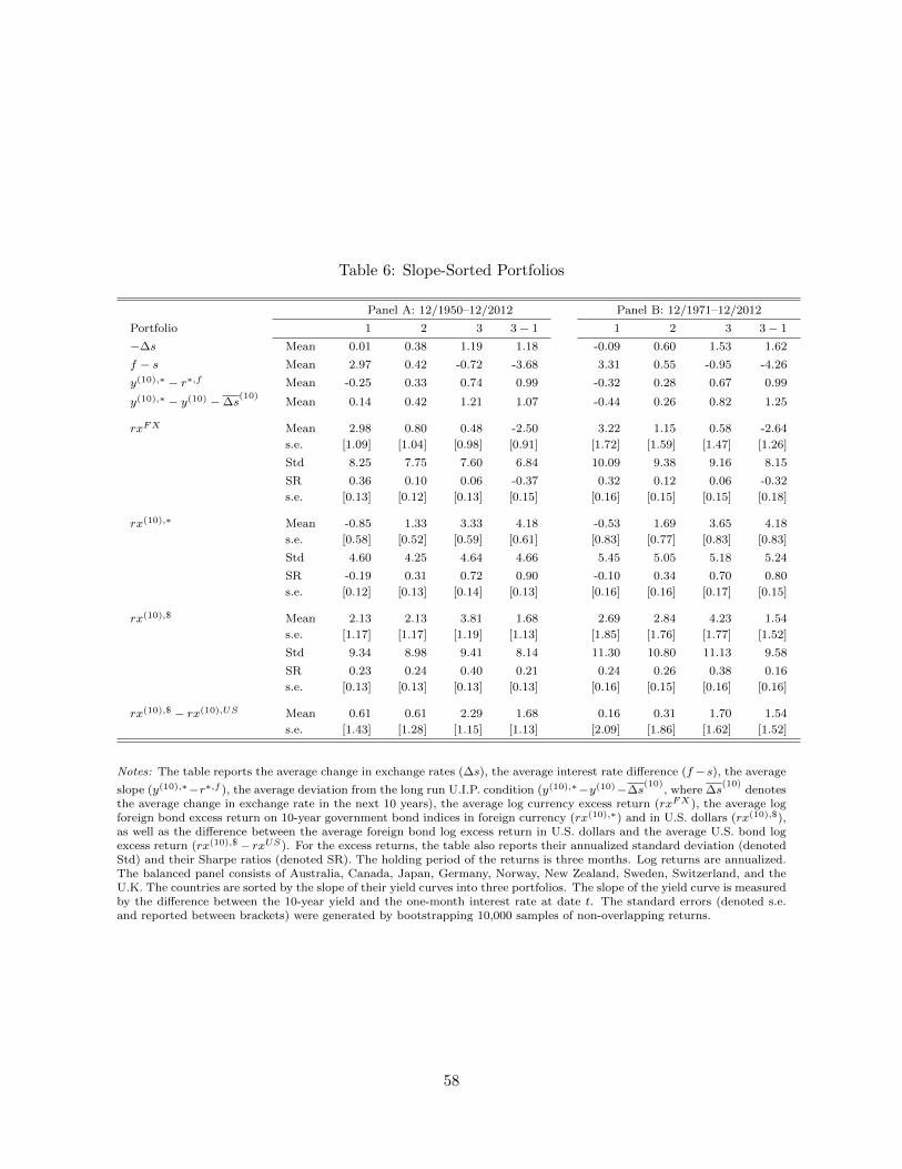
Table 6: Slope-Sorted Portfolios

Panel A: 12/1950–12/2012 Panel B: 12/1971–12/2012

Portfolio 1 2 3 3− 1 1 2 3 3− 1

−∆s Mean 0.01 0.38 1.19 1.18 -0.09 0.60 1.53 1.62

f − s Mean 2.97 0.42 -0.72 -3.68 3.31 0.55 -0.95 -4.26

y(10),∗ − r∗,f Mean -0.25 0.33 0.74 0.99 -0.32 0.28 0.67 0.99

y(10),∗ − y(10) −∆s(10)

Mean 0.14 0.42 1.21 1.07 -0.44 0.26 0.82 1.25

rxFX Mean 2.98 0.80 0.48 -2.50 3.22 1.15 0.58 -2.64

s.e. [1.09] [1.04] [0.98] [0.91] [1.72] [1.59] [1.47] [1.26]

Std 8.25 7.75 7.60 6.84 10.09 9.38 9.16 8.15

SR 0.36 0.10 0.06 -0.37 0.32 0.12 0.06 -0.32

s.e. [0.13] [0.12] [0.13] [0.15] [0.16] [0.15] [0.15] [0.18]

rx(10),∗ Mean -0.85 1.33 3.33 4.18 -0.53 1.69 3.65 4.18

s.e. [0.58] [0.52] [0.59] [0.61] [0.83] [0.77] [0.83] [0.83]

Std 4.60 4.25 4.64 4.66 5.45 5.05 5.18 5.24

SR -0.19 0.31 0.72 0.90 -0.10 0.34 0.70 0.80

s.e. [0.12] [0.13] [0.14] [0.13] [0.16] [0.16] [0.17] [0.15]

rx(10),$ Mean 2.13 2.13 3.81 1.68 2.69 2.84 4.23 1.54

s.e. [1.17] [1.17] [1.19] [1.13] [1.85] [1.76] [1.77] [1.52]

Std 9.34 8.98 9.41 8.14 11.30 10.80 11.13 9.58

SR 0.23 0.24 0.40 0.21 0.24 0.26 0.38 0.16

s.e. [0.13] [0.13] [0.13] [0.13] [0.16] [0.15] [0.16] [0.16]

rx(10),$ − rx(10),US Mean 0.61 0.61 2.29 1.68 0.16 0.31 1.70 1.54

s.e. [1.43] [1.28] [1.15] [1.13] [2.09] [1.86] [1.62] [1.52]

Notes: The table reports the average change in exchange rates (∆s), the average interest rate difference (f −s), the average

slope (y(10),∗−r∗,f ), the average deviation from the long run U.I.P. condition (y(10),∗−y(10)−∆s(10)

, where ∆s(10)

denotesthe average change in exchange rate in the next 10 years), the average log currency excess return (rxFX), the average logforeign bond excess return on 10-year government bond indices in foreign currency (rx(10),∗) and in U.S. dollars (rx(10),$),as well as the difference between the average foreign bond log excess return in U.S. dollars and the average U.S. bond logexcess return (rx(10),$− rxUS). For the excess returns, the table also reports their annualized standard deviation (denotedStd) and their Sharpe ratios (denoted SR). The holding period of the returns is three months. Log returns are annualized.The balanced panel consists of Australia, Canada, Japan, Germany, Norway, New Zealand, Sweden, Switzerland, and theU.K. The countries are sorted by the slope of their yield curves into three portfolios. The slope of the yield curve is measuredby the difference between the 10-year yield and the one-month interest rate at date t. The standard errors (denoted s.e.and reported between brackets) were generated by bootstrapping 10,000 samples of non-overlapping returns.

58

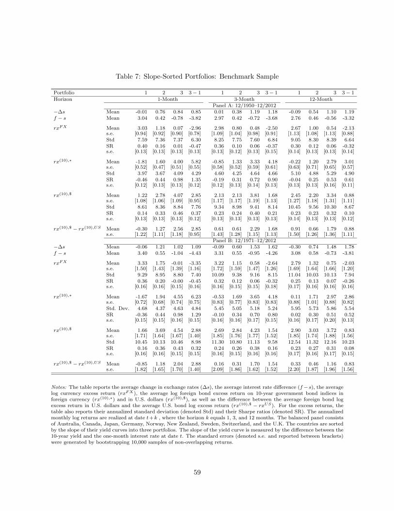
Table 7: Slope-Sorted Portfolios: Benchmark Sample

Portfolio 1 2 3 3− 1 1 2 3 3− 1 1 2 3 3− 1

Horizon 1-Month 3-Month 12-MonthPanel A: 12/1950–12/2012

−∆s Mean -0.01 0.76 0.84 0.85 0.01 0.38 1.19 1.18 -0.09 0.54 1.10 1.19f − s Mean 3.04 0.42 -0.78 -3.82 2.97 0.42 -0.72 -3.68 2.76 0.46 -0.56 -3.32

rxFX Mean 3.03 1.18 0.07 -2.96 2.98 0.80 0.48 -2.50 2.67 1.00 0.54 -2.13s.e. [0.94] [0.92] [0.90] [0.78] [1.09] [1.04] [0.98] [0.91] [1.13] [1.08] [1.13] [0.88]Std 7.59 7.36 7.37 6.30 8.25 7.75 7.60 6.84 9.05 8.30 8.39 6.64SR 0.40 0.16 0.01 -0.47 0.36 0.10 0.06 -0.37 0.30 0.12 0.06 -0.32s.e. [0.13] [0.13] [0.13] [0.13] [0.13] [0.12] [0.13] [0.15] [0.14] [0.13] [0.13] [0.14]

rx(10),∗ Mean -1.81 1.60 4.00 5.82 -0.85 1.33 3.33 4.18 -0.22 1.20 2.79 3.01s.e. [0.52] [0.47] [0.51] [0.55] [0.58] [0.52] [0.59] [0.61] [0.63] [0.71] [0.65] [0.57]Std 3.97 3.67 4.09 4.29 4.60 4.25 4.64 4.66 5.10 4.88 5.29 4.90SR -0.46 0.44 0.98 1.35 -0.19 0.31 0.72 0.90 -0.04 0.25 0.53 0.61s.e. [0.12] [0.13] [0.13] [0.12] [0.12] [0.13] [0.14] [0.13] [0.13] [0.13] [0.16] [0.11]

rx(10),$ Mean 1.22 2.78 4.07 2.85 2.13 2.13 3.81 1.68 2.45 2.20 3.34 0.88s.e. [1.08] [1.06] [1.09] [0.95] [1.17] [1.17] [1.19] [1.13] [1.27] [1.18] [1.31] [1.11]Std 8.61 8.36 8.84 7.76 9.34 8.98 9.41 8.14 10.45 9.56 10.30 8.67SR 0.14 0.33 0.46 0.37 0.23 0.24 0.40 0.21 0.23 0.23 0.32 0.10s.e. [0.13] [0.13] [0.13] [0.12] [0.13] [0.13] [0.13] [0.13] [0.14] [0.13] [0.13] [0.12]

rx(10),$ − rx(10),US Mean -0.30 1.27 2.56 2.85 0.61 0.61 2.29 1.68 0.91 0.66 1.79 0.88s.e. [1.22] [1.11] [1.18] [0.95] [1.43] [1.28] [1.15] [1.13] [1.50] [1.26] [1.36] [1.11]

Panel B: 12/1971–12/2012−∆s Mean -0.06 1.21 1.02 1.09 -0.09 0.60 1.53 1.62 -0.30 0.74 1.48 1.78f − s Mean 3.40 0.55 -1.04 -4.43 3.31 0.55 -0.95 -4.26 3.08 0.58 -0.73 -3.81

rxFX Mean 3.33 1.75 -0.01 -3.35 3.22 1.15 0.58 -2.64 2.79 1.32 0.75 -2.03s.e. [1.50] [1.43] [1.39] [1.16] [1.72] [1.59] [1.47] [1.26] [1.69] [1.64] [1.66] [1.20]Std 9.29 8.95 8.80 7.40 10.09 9.38 9.16 8.15 11.04 10.03 10.13 7.94SR 0.36 0.20 -0.00 -0.45 0.32 0.12 0.06 -0.32 0.25 0.13 0.07 -0.26s.e. [0.16] [0.16] [0.15] [0.16] [0.16] [0.15] [0.15] [0.18] [0.17] [0.16] [0.16] [0.16]

rx(10),∗ Mean -1.67 1.94 4.55 6.23 -0.53 1.69 3.65 4.18 0.11 1.71 2.97 2.86s.e. [0.72] [0.68] [0.74] [0.75] [0.83] [0.77] [0.83] [0.83] [0.88] [1.01] [0.88] [0.82]Std. Dev. 4.68 4.37 4.63 4.84 5.45 5.05 5.18 5.24 5.95 5.73 5.86 5.54SR -0.36 0.44 0.98 1.29 -0.10 0.34 0.70 0.80 0.02 0.30 0.51 0.52s.e. [0.15] [0.15] [0.16] [0.15] [0.16] [0.16] [0.17] [0.15] [0.16] [0.17] [0.20] [0.13]

rx(10),$ Mean 1.66 3.69 4.54 2.88 2.69 2.84 4.23 1.54 2.90 3.03 3.72 0.83s.e. [1.71] [1.64] [1.67] [1.40] [1.85] [1.76] [1.77] [1.52] [1.85] [1.74] [1.88] [1.56]Std 10.45 10.13 10.46 8.98 11.30 10.80 11.13 9.58 12.54 11.32 12.16 10.23SR 0.16 0.36 0.43 0.32 0.24 0.26 0.38 0.16 0.23 0.27 0.31 0.08s.e. [0.16] [0.16] [0.15] [0.15] [0.16] [0.15] [0.16] [0.16] [0.17] [0.16] [0.17] [0.15]

rx(10),$ − rx(10),US Mean -0.85 1.18 2.04 2.88 0.16 0.31 1.70 1.54 0.33 0.46 1.16 0.83s.e. [1.82] [1.65] [1.70] [1.40] [2.09] [1.86] [1.62] [1.52] [2.20] [1.87] [1.96] [1.56]

Notes: The table reports the average change in exchange rates (∆s), the average interest rate difference (f −s), the averagelog currency excess return (rxFX), the average log foreign bond excess return on 10-year government bond indices inforeign currency (rx(10),∗) and in U.S. dollars (rx(10),$), as well as the difference between the average foreign bond logexcess return in U.S. dollars and the average U.S. bond log excess return (rx(10),$ − rxUS). For the excess returns, thetable also reports their annualized standard deviation (denoted Std) and their Sharpe ratios (denoted SR). The annualizedmonthly log returns are realized at date t+k , where the horizon k equals 1, 3, and 12 months. The balanced panel consistsof Australia, Canada, Japan, Germany, Norway, New Zealand, Sweden, Switzerland, and the U.K. The countries are sortedby the slope of their yield curves into three portfolios. The slope of the yield curve is measured by the difference between the10-year yield and the one-month interest rate at date t. The standard errors (denoted s.e. and reported between brackets)were generated by bootstrapping 10,000 samples of non-overlapping returns.

59

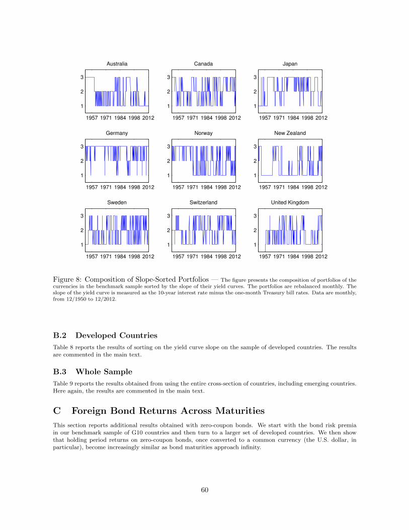
1957 1971 1984 1998 2012

1

2

3

Australia

1957 1971 1984 1998 2012

1

2

3

Canada

1957 1971 1984 1998 2012

1

2

3

Japan

1957 1971 1984 1998 2012

1

2

3

Germany

1957 1971 1984 1998 2012

1

2

3

Norway

1957 1971 1984 1998 2012

1

2

3

New Zealand

1957 1971 1984 1998 2012

1

2

3

Sweden

1957 1971 1984 1998 2012

1

2

3

Switzerland

1957 1971 1984 1998 2012

1

2

3

United Kingdom

Figure 8: Composition of Slope-Sorted Portfolios — The figure presents the composition of portfolios of thecurrencies in the benchmark sample sorted by the slope of their yield curves. The portfolios are rebalanced monthly. Theslope of the yield curve is measured as the 10-year interest rate minus the one-month Treasury bill rates. Data are monthly,from 12/1950 to 12/2012.

B.2 Developed Countries

Table 8 reports the results of sorting on the yield curve slope on the sample of developed countries. The resultsare commented in the main text.

B.3 Whole Sample

Table 9 reports the results obtained from using the entire cross-section of countries, including emerging countries.Here again, the results are commented in the main text.

C Foreign Bond Returns Across Maturities

This section reports additional results obtained with zero-coupon bonds. We start with the bond risk premiain our benchmark sample of G10 countries and then turn to a larger set of developed countries. We then showthat holding period returns on zero-coupon bonds, once converted to a common currency (the U.S. dollar, inparticular), become increasingly similar as bond maturities approach infinity.

60

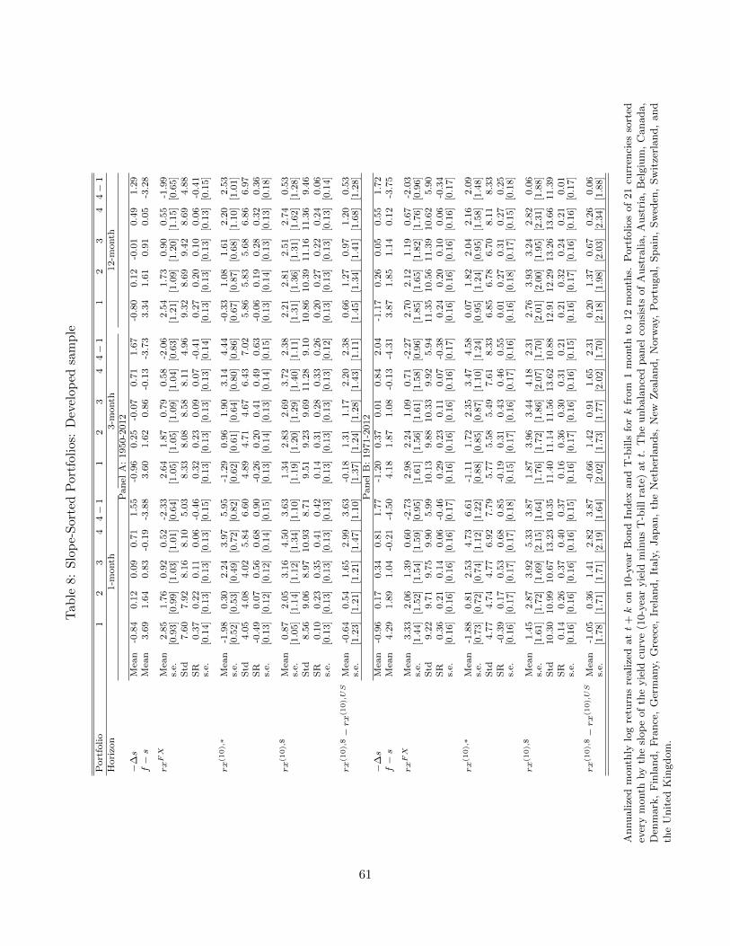
Tab

le8:

Slo

pe-

Sor

ted

Por

tfol

ios:

Dev

elop

edsa

mp

le

Port

folio

12

34

4−

11

23

44−

11

23

44−

1H

ori

zon

1-m

onth

3-m

onth

12-m

onth

Pan

elA

:1950-2

012

−∆s

Mea

n-0

.84

0.1

20.0

90.7

11.5

5-0

.96

0.2

5-0

.07

0.7

11.6

7-0

.80

0.1

2-0

.01

0.4

91.2

9f−s

Mea

n3.6

91.6

40.8

3-0

.19

-3.8

83.6

01.6

20.8

6-0

.13

-3.7

33.3

41.6

10.9

10.0

5-3

.28

rxFX

Mea

n2.8

51.7

60.9

20.5

2-2

.33

2.6

41.8

70.7

90.5

8-2

.06

2.5

41.7

30.9

00.5

5-1

.99

s.e.

[0.9

3]

[0.9

9]

[1.0

3]

[1.0

1]

[0.6

4]

[1.0

5]

[1.0

5]

[1.0

9]

[1.0

4]

[0.6

3]

[1.2

1]

[1.0

9]

[1.2

0]

[1.1

5]

[0.6

5]

Std

7.6

07.9

28.1

68.1

05.0

38.3

38.0

88.5

88.1

14.9

69.3

28.6

99.4

28.6

94.8

8S

R0.3

70.2

20.1

10.0

6-0

.46

0.3

20.2

30.0

90.0

7-0

.41

0.2

70.2

00.1

00.0

6-0

.41

s.e.

[0.1

4]

[0.1

3]

[0.1

3]

[0.1

3]

[0.1

5]

[0.1

3]

[0.1

3]

[0.1

3]

[0.1

3]

[0.1

4]

[0.1

3]

[0.1

3]

[0.1

3]

[0.1

3]

[0.1

5]

rx

(10),∗

Mea

n-1

.98

0.3

02.2

43.9

75.9

5-1

.29

0.9

61.9

03.1

44.4

4-0

.33

1.0

81.6

12.2

02.5

3s.

e.[0

.52]

[0.5

3]

[0.4

9]

[0.7

2]

[0.8

2]

[0.6

2]

[0.6

1]

[0.6

4]

[0.8

0]

[0.8

6]

[0.6

7]

[0.8

7]

[0.6

8]

[1.1

0]

[1.0

1]

Std

4.0

54.0

84.0

25.8

46.6

04.8

94.7

14.6

76.4

37.0

25.8

65.8

35.6

86.8

66.9

7S

R-0

.49

0.0

70.5

60.6

80.9

0-0

.26

0.2

00.4

10.4

90.6

3-0

.06

0.1

90.2

80.3

20.3

6s.

e.[0

.13]

[0.1

2]

[0.1

2]

[0.1

4]

[0.1

5]

[0.1

3]

[0.1

4]

[0.1

3]

[0.1

4]

[0.1

5]

[0.1

3]

[0.1

4]

[0.1

3]

[0.1

3]

[0.1

8]

rx

(10),

$M

ean

0.8

72.0

53.1

64.5

03.6

31.3

42.8

32.6

93.7

22.3

82.2

12.8

12.5

12.7

40.5

3s.

e.[1

.05]

[1.1

4]

[1.1

2]

[1.3

4]

[1.1

0]

[1.1

9]

[1.2

0]

[1.2

9]

[1.4

0]

[1.1

1]

[1.3

1]

[1.3

6]

[1.3

1]

[1.6

2]

[1.2

8]

Std

8.5

69.0

68.9

710.9

38.7

19.5

19.2

39.6

911.2

89.1

010.8

610.3

911.1

611.3

69.4

6S

R0.1

00.2

30.3

50.4

10.4

20.1

40.3

10.2

80.3

30.2

60.2

00.2

70.2

20.2

40.0

6s.

e.[0

.13]

[0.1

3]

[0.1

3]

[0.1

3]

[0.1

3]

[0.1

3]

[0.1

3]

[0.1

3]

[0.1

3]

[0.1

2]

[0.1

3]

[0.1

3]

[0.1

3]

[0.1

3]

[0.1

4]

rx

(10),

$−rx

(10),US

Mea

n-0

.64

0.5

41.6

52.9

93.6

3-0

.18

1.3

11.1

72.2

02.3

80.6

61.2

70.9

71.2

00.5

3s.

e.[1

.23]

[1.2

1]

[1.2

1]

[1.4

7]

[1.1

0]

[1.3

7]

[1.2

4]

[1.2

8]

[1.4

3]

[1.1

1]

[1.4

5]

[1.3

4]

[1.4

1]

[1.6

8]

[1.2

8]

Pan

elB

:1971-2

012

−∆s

Mea

n-0

.96

0.1

70.3

40.8

11.7

7-1

.20

0.3

70.0

10.8

42.0

4-1

.17

0.2

60.0

50.5

51.7

2f−s

Mea

n4.2

91.8

91.0

4-0

.21

-4.5

04.1

81.8

71.0

8-0

.13

-4.3

13.8

71.8

51.1

40.1

2-3

.75

rxFX

Mea

n3.3

32.0

61.3

90.6

0-2

.73

2.9

82.2

41.0

90.7

1-2

.27

2.7

02.1

21.1

90.6

7-2

.03

s.e.

[1.4

4]

[1.5

2]

[1.5

4]

[1.5

9]

[0.9

5]

[1.6

1]

[1.5

6]

[1.6

1]

[1.5

8]

[0.9

6]

[1.8

5]

[1.6

5]

[1.8

2]

[1.7

6]

[0.9

6]

Std

9.2

29.7

19.7

59.9

05.9

910.1

39.8

810.3

39.9

25.9

411.3

510.5

611.3

910.6

25.9

0S

R0.3

60.2

10.1

40.0

6-0

.46

0.2

90.2

30.1

10.0

7-0

.38

0.2

40.2

00.1

00.0

6-0

.34

s.e.

[0.1

6]

[0.1

6]

[0.1

6]

[0.1

6]

[0.1

7]

[0.1

6]

[0.1

6]

[0.1

6]

[0.1

6]

[0.1

7]

[0.1

6]

[0.1

6]

[0.1

6]

[0.1

6]

[0.1

7]

rx

(10),∗

Mea

n-1

.88

0.8

12.5

34.7

36.6

1-1

.11

1.7

22.3

53.4

74.5

80.0

71.8

22.0

42.1

62.0

9s.

e.[0

.73]

[0.7

2]

[0.7

4]

[1.1

2]

[1.2

2]

[0.8

8]

[0.8

5]

[0.8

7]

[1.1

0]

[1.2

4]

[0.9

5]

[1.2

4]

[0.9

5]

[1.5

8]

[1.4

8]

Std

4.7

74.7

44.7

76.9

27.7

95.7

75.5

85.4

97.6

18.3

36.8

56.7

86.7

08.1

18.3

3S

R-0

.39

0.1

70.5

30.6

80.8

5-0

.19

0.3

10.4

30.4

60.5

50.0

10.2

70.3

10.2

70.2

5s.

e.[0

.16]

[0.1

7]

[0.1

7]

[0.1

7]

[0.1

8]

[0.1

5]

[0.1

7]

[0.1

6]

[0.1

7]

[0.1

6]

[0.1

6]

[0.1

8]

[0.1

7]

[0.1

5]

[0.1

8]

rx

(10),

$M

ean

1.4

52.8

73.9

25.3

33.8

71.8

73.9

63.4

44.1

82.3

12.7

63.9

33.2

42.8

20.0

6s.

e.[1

.61]

[1.7

2]

[1.6

9]

[2.1

5]

[1.6

4]

[1.7

6]

[1.7

2]

[1.8

6]

[2.0

7]

[1.7

0]

[2.0

1]

[2.0

0]

[1.9

5]

[2.3

1]

[1.8

8]

Std

10.3

010.9

910.6

713.2

310.3

511.4

011.1

411.5

613.6

210.8

812.9

112.2

913.2

613.6

611.3

9S

R0.1

40.2

60.3

70.4

00.3

70.1

60.3

60.3

00.3

10.2

10.2

10.3

20.2

40.2

10.0

1s.

e.[0

.16]

[0.1

6]

[0.1

6]

[0.1

6]

[0.1

5]

[0.1

6]

[0.1

7]

[0.1

6]

[0.1

6]

[0.1

5]

[0.1

6]

[0.1

7]

[0.1

6]

[0.1

6]

[0.1

7]

rx

(10),

$−rx

(10),US

Mea

n-1

.05

0.3

61.4

12.8

23.8

7-0

.66

1.4

20.9

11.6

52.3

10.2

01.3

70.6

70.2

60.0

6s.

e.[1

.78]

[1.7

1]

[1.7

1]

[2.1

9]

[1.6

4]

[2.0

2]

[1.7

3]

[1.7

7]

[2.0

2]

[1.7

0]

[2.1

8]

[1.9

8]

[2.0

3]

[2.3

4]

[1.8

8]

Annualize

dm

onth

lylo

gre

turn

sre

alize

datt

+k

on

10-y

ear

Bond

Index

and

T-b

ills

fork

from

1m

onth

to12

month

s.P

ort

folios

of

21

curr

enci

esso

rted

ever

ym

onth

by

the

slop

eof

the

yie

ldcu

rve

(10-y

ear

yie

ldm

inus

T-b

ill

rate

)att.

The

unbala

nce

dpanel

consi

sts

of

Aust

ralia,

Aust

ria,

Bel

giu

m,

Canada,

Den

mark

,F

inla

nd,

Fra

nce

,G

erm

any,

Gre

ece,

Irel

and,

Italy

,Japan,

the

Net

her

lands,

New

Zea

land,

Norw

ay,

Port

ugal,

Spain

,Sw

eden

,Sw

itze

rland,

and

the

Unit

edK

ingdom

.

61

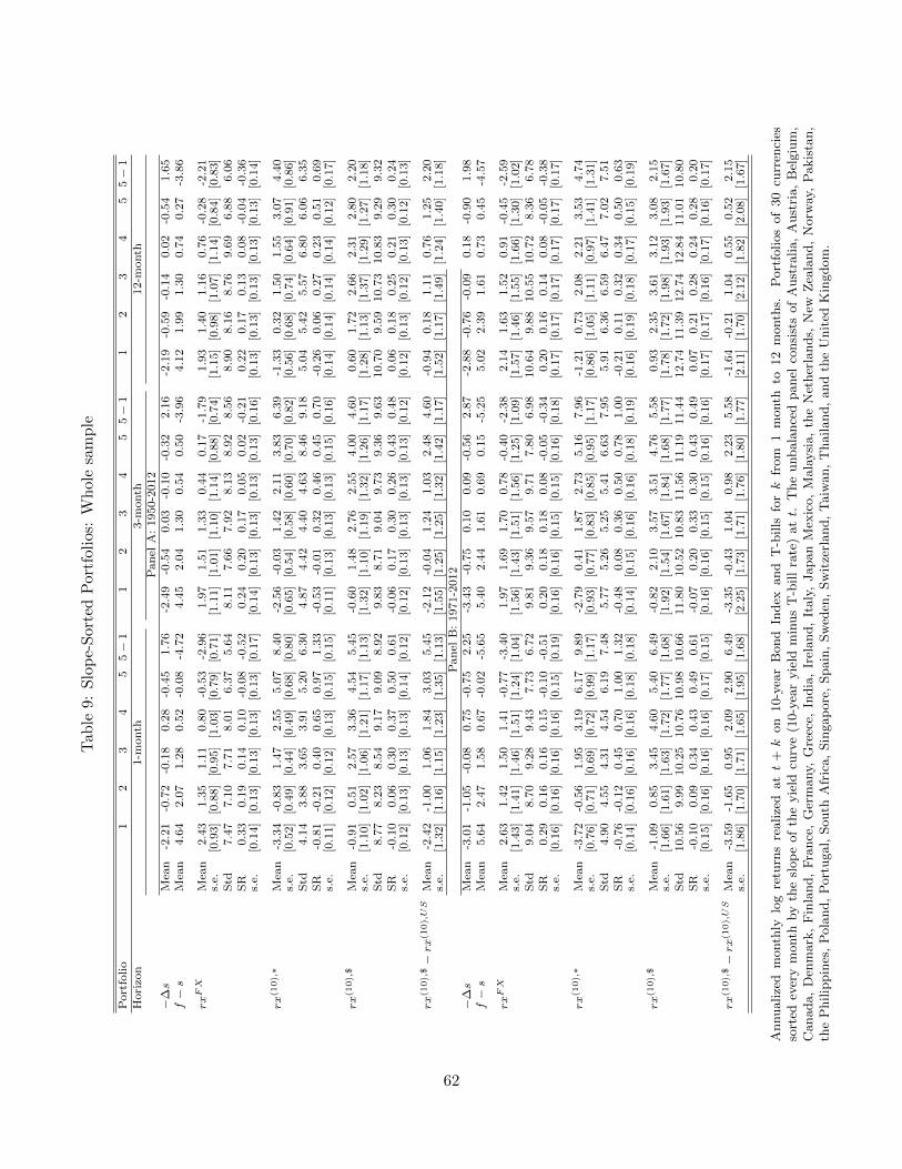
Tab

le9:

Slo

pe-

Sor

ted

Por

tfol

ios:

Wh

ole

sam

ple

Port

folio

12

34

55−

11

23

45

5−

11

23

45

5−

1H

ori

zon

1-m

onth

3-m

onth

12-m

onth

Pan

elA

:1950-2

012

−∆s

Mea

n-2

.21

-0.7

2-0

.18

0.2

8-0

.45

1.7

6-2

.49

-0.5

40.0

3-0

.10

-0.3

22.1

6-2

.19

-0.5

9-0

.14

0.0

2-0

.54

1.6

5f−s

Mea

n4.6

42.0

71.2

80.5

2-0

.08

-4.7

24.4

52.0

41.3

00.5

40.5

0-3

.96

4.1

21.9

91.3

00.7

40.2

7-3

.86

rxFX

Mea

n2.4

31.3

51.1

10.8

0-0

.53

-2.9

61.9

71.5

11.3

30.4

40.1

7-1

.79

1.9

31.4

01.1

60.7

6-0

.28

-2.2

1s.

e.[0

.93]

[0.8

8]

[0.9

5]

[1.0

3]

[0.7

9]

[0.7

1]

[1.1

1]

[1.0

1]

[1.1

0]

[1.1

4]

[0.8

8]

[0.7

4]

[1.1

5]

[0.9

8]

[1.0

7]

[1.1

4]

[0.8

4]

[0.8

3]

Std

7.4

77.1

07.7

18.0

16.3

75.6

48.1

17.6

67.9

28.1

38.9

28.5

68.9

08.1

68.7

69.6

96.8

86.0

6S

R0.3

30.1

90.1

40.1

0-0

.08

-0.5

20.2

40.2

00.1

70.0

50.0

2-0

.21

0.2

20.1

70.1

30.0

8-0

.04

-0.3

6s.

e.[0

.14]

[0.1

3]

[0.1

3]

[0.1

3]

[0.1

3]

[0.1

7]

[0.1

4]

[0.1

3]

[0.1

3]

[0.1

3]

[0.1

3]

[0.1

6]

[0.1

3]

[0.1

3]

[0.1

3]

[0.1

3]

[0.1

3]

[0.1

4]

rx

(10),∗

Mea

n-3

.34

-0.8

31.4

72.5

55.0

78.4

0-2

.56

-0.0

31.4

22.1

13.8

36.3

9-1

.33

0.3

21.5

01.5

53.0

74.4

0s.

e.[0

.52]

[0.4

9]

[0.4

4]

[0.4

9]

[0.6

8]

[0.8

0]

[0.6

5]

[0.5

4]

[0.5

8]

[0.6

0]

[0.7

0]

[0.8

2]

[0.5

6]

[0.6

8]

[0.7

4]

[0.6

4]

[0.9

1]

[0.8

6]

Std

4.1

43.8

83.6

53.9

15.2

06.3

04.8

74.4

24.4

04.6

38.4

69.1

85.0

45.4

25.5

76.8

06.0

66.3

5S

R-0

.81

-0.2

10.4

00.6

50.9

71.3

3-0

.53

-0.0

10.3

20.4

60.4

50.7

0-0

.26

0.0

60.2

70.2

30.5

10.6

9s.

e.[0

.11]

[0.1

2]

[0.1

2]

[0.1

3]

[0.1

5]

[0.1

5]

[0.1

1]

[0.1

3]

[0.1

3]

[0.1

3]

[0.1

5]

[0.1

6]

[0.1

4]

[0.1

4]

[0.1

4]

[0.1

4]

[0.1

2]

[0.1

7]

rx

(10),

$M

ean

-0.9

10.5

12.5

73.3

64.5

45.4

5-0

.60

1.4

82.7

62.5

54.0

04.6

00.6

01.7

22.6

62.3

12.8

02.2

0s.

e.[1

.10]

[1.0

2]

[1.0

6]

[1.2

1]

[1.1

7]

[1.1

3]

[1.3

2]

[1.1

0]

[1.1

9]

[1.3

2]

[1.2

6]

[1.1

7]

[1.2

8]

[1.1

3]

[1.3

7]

[1.2

9]

[1.2

7]

[1.1

8]

Std

8.7

78.2

38.5

49.1

79.0

98.9

29.8

38.7

19.0

49.7

39.3

69.6

310.7

09.5

910.7

310.8

39.2

99.3

2S

R-0

.10

0.0

60.3

00.3

70.5

00.6

1-0

.06

0.1

70.3

00.2

60.4

30.4

80.0

60.1

80.2

50.2

10.3

00.2

4s.

e.[0

.12]

[0.1

3]

[0.1

3]

[0.1

3]

[0.1

4]

[0.1

2]

[0.1

2]

[0.1

3]

[0.1

3]

[0.1

3]

[0.1

3]

[0.1

2]

[0.1

2]

[0.1

3]

[0.1

2]

[0.1

3]

[0.1

2]

[0.1

3]

rx

(10),

$−rx

(10),US

Mea

n-2

.42

-1.0

01.0

61.8

43.0

35.4

5-2

.12

-0.0

41.2

41.0

32.4

84.6

0-0

.94

0.1

81.1

10.7

61.2

52.2

0s.

e.[1

.32]

[1.1

6]

[1.1

5]

[1.2

3]

[1.3

5]

[1.1

3]

[1.5

5]

[1.2

5]

[1.2

5]

[1.3

2]

[1.4

2]

[1.1

7]

[1.5

2]

[1.1

7]

[1.4

9]

[1.2

4]

[1.4

0]

[1.1

8]

Pan

elB

:1971-2

012

−∆s

Mea

n-3

.01

-1.0

5-0

.08

0.7

5-0

.75

2.2

5-3

.43

-0.7

50.1

00.0

9-0

.56

2.8

7-2

.88

-0.7

6-0

.09

0.1

8-0

.90

1.9

8f−s

Mea

n5.6

42.4

71.5

80.6

7-0

.02

-5.6

55.4

02.4

41.6

10.6

90.1

5-5

.25

5.0

22.3

91.6

10.7

30.4

5-4

.57

rxFX

Mea

n2.6

31.4

21.5

01.4

1-0

.77

-3.4

01.9

71.6

91.7

00.7

8-0

.40

-2.3

82.1

41.6

31.5

20.9

1-0

.45

-2.5

9s.

e.[1

.43]

[1.4

1]

[1.4

6]

[1.5

1]

[1.2

4]

[1.0

4]

[1.5

6]

[1.4

3]

[1.5

1]

[1.5

6]

[1.2

5]

[1.0

9]

[1.5

7]

[1.4

6]

[1.5

5]

[1.6

6]

[1.3

0]

[1.0

2]

Std

9.0

48.7

09.2

89.4

37.7

36.7

29.8

19.3

69.5

79.7

17.8

06.9

810.6

49.8

810.5

510.7

28.3

66.7

8S

R0.2

90.1

60.1

60.1

5-0

.10

-0.5

10.2

00.1

80.1

80.0

8-0

.05

-0.3

40.2

00.1

60.1

40.0

8-0

.05

-0.3

8s.

e.[0

.16]

[0.1

6]

[0.1

6]

[0.1

6]

[0.1

5]

[0.1

9]

[0.1

6]

[0.1

6]

[0.1

5]

[0.1

5]

[0.1

6]

[0.1

8]

[0.1

7]

[0.1

7]

[0.1

7]

[0.1

7]

[0.1

7]

[0.1

7]

rx

(10),∗

Mea

n-3

.72

-0.5

61.9

53.1

96.1

79.8

9-2

.79

0.4

11.8

72.7

35.1

67.9

6-1

.21

0.7

32.0

82.2

13.5

34.7

4s.

e.[0

.76]

[0.7

1]

[0.6

9]

[0.7

2]

[0.9

9]

[1.1

7]

[0.9

3]

[0.7

7]

[0.8

3]

[0.8

5]

[0.9

5]

[1.1

7]

[0.8

6]

[1.0

5]

[1.1

1]

[0.9

7]

[1.4

1]

[1.3

1]

Std

4.9

04.5

54.3

14.5

46.1

97.4

85.7

75.2

65.2

55.4

16.6

37.9

55.9

16.3

66.5

96.4

77.0

27.5

1S

R-0

.76

-0.1

20.4

50.7

01.0

01.3

2-0

.48

0.0

80.3

60.5

00.7

81.0

0-0

.21

0.1

10.3

20.3

40.5

00.6

3s.

e.[0

.14]

[0.1

6]

[0.1

6]

[0.1

6]

[0.1

8]

[0.1

8]

[0.1

4]

[0.1

5]

[0.1

6]

[0.1

6]

[0.1

8]

[0.1

9]

[0.1

6]

[0.1

9]

[0.1

8]

[0.1

7]

[0.1

5]

[0.1

9]

rx

(10),

$M

ean

-1.0

90.8

53.4

54.6

05.4

06.4

9-0

.82

2.1

03.5

73.5

14.7

65.5

80.9

32.3

53.6

13.1

23.0

82.1

5s.

e.[1

.66]

[1.6

1]

[1.6

3]

[1.7

2]

[1.7

7]

[1.6

8]

[1.9

2]

[1.5

4]

[1.6

7]

[1.8

4]

[1.6

8]

[1.7

7]

[1.7

8]

[1.7

2]

[1.9

8]

[1.9

3]

[1.9

3]

[1.6

7]

Std

10.5

69.9

910.2

510.7

610.9

810.6

611.8

010.5

210.8

311.5

611.1

911.4

412.7

411.3

912.7

412.8

411.0

110.8

0S

R-0

.10

0.0

90.3

40.4

30.4

90.6

1-0

.07

0.2

00.3

30.3

00.4

30.4

90.0

70.2

10.2

80.2

40.2

80.2

0s.

e.[0

.15]

[0.1

6]

[0.1

6]

[0.1

6]

[0.1

7]

[0.1

5]

[0.1

6]

[0.1

6]

[0.1

5]

[0.1

5]

[0.1

6]

[0.1

6]

[0.1

7]

[0.1

7]

[0.1

6]

[0.1

7]

[0.1

6]

[0.1

7]

rx

(10),

$−rx

(10),US

Mea

n-3

.59

-1.6

50.9

52.0

92.9

06.4

9-3

.35

-0.4

31.0

40.9

82.2

35.5

8-1

.64

-0.2

11.0

40.5

50.5

22.1

5s.

e.[1

.86]

[1.7

0]

[1.7

1]

[1.6

5]

[1.9

5]

[1.6

8]

[2.2

5]

[1.7

3]

[1.7

1]

[1.7

6]

[1.8

0]

[1.7

7]

[2.1

1]

[1.7

0]

[2.1

2]

[1.8

2]

[2.0

8]

[1.6

7]

Annualize

dm

onth

lylo

gre

turn

sre

alize

datt

+k

on

10-y

ear

Bond

Index

and

T-b

ills

fork

from

1m

onth

to12

month

s.P

ort

folios

of

30

curr

enci

esso

rted

ever

ym

onth

by

the

slop

eof

the

yie

ldcu

rve

(10-y

ear

yie

ldm

inus

T-b

ill

rate

)att.

The

unbala

nce

dpanel

consi

sts

of

Aust

ralia,

Aust

ria,

Bel

giu

m,

Canada,

Den

mark

,F

inla

nd,

Fra

nce

,G

erm

any,

Gre

ece,

India

,Ir

eland,

Italy

,Japan

Mex

ico,

Mala

ysi

a,

the

Net

her

lands,

New

Zea

land,

Norw

ay,

Pakis

tan,

the

Philip

pin

es,

Pola

nd,

Port

ugal,

South

Afr

ica,

Sin

gap

ore

,Spain

,Sw

eden

,Sw

itze

rland,

Taiw

an,

Thailand,

and

the

Unit

edK

ingdom

.

62

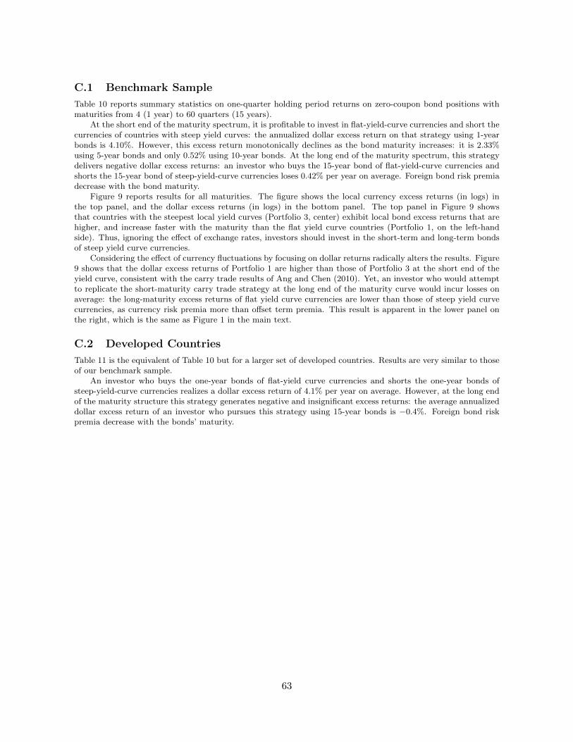
C.1 Benchmark Sample

Table 10 reports summary statistics on one-quarter holding period returns on zero-coupon bond positions withmaturities from 4 (1 year) to 60 quarters (15 years).

At the short end of the maturity spectrum, it is profitable to invest in flat-yield-curve currencies and short thecurrencies of countries with steep yield curves: the annualized dollar excess return on that strategy using 1-yearbonds is 4.10%. However, this excess return monotonically declines as the bond maturity increases: it is 2.33%using 5-year bonds and only 0.52% using 10-year bonds. At the long end of the maturity spectrum, this strategydelivers negative dollar excess returns: an investor who buys the 15-year bond of flat-yield-curve currencies andshorts the 15-year bond of steep-yield-curve currencies loses 0.42% per year on average. Foreign bond risk premiadecrease with the bond maturity.

Figure 9 reports results for all maturities. The figure shows the local currency excess returns (in logs) inthe top panel, and the dollar excess returns (in logs) in the bottom panel. The top panel in Figure 9 showsthat countries with the steepest local yield curves (Portfolio 3, center) exhibit local bond excess returns that arehigher, and increase faster with the maturity than the flat yield curve countries (Portfolio 1, on the left-handside). Thus, ignoring the effect of exchange rates, investors should invest in the short-term and long-term bondsof steep yield curve currencies.

Considering the effect of currency fluctuations by focusing on dollar returns radically alters the results. Figure9 shows that the dollar excess returns of Portfolio 1 are higher than those of Portfolio 3 at the short end of theyield curve, consistent with the carry trade results of Ang and Chen (2010). Yet, an investor who would attemptto replicate the short-maturity carry trade strategy at the long end of the maturity curve would incur losses onaverage: the long-maturity excess returns of flat yield curve currencies are lower than those of steep yield curvecurrencies, as currency risk premia more than offset term premia. This result is apparent in the lower panel onthe right, which is the same as Figure 1 in the main text.

C.2 Developed Countries

Table 11 is the equivalent of Table 10 but for a larger set of developed countries. Results are very similar to thoseof our benchmark sample.

An investor who buys the one-year bonds of flat-yield curve currencies and shorts the one-year bonds ofsteep-yield-curve currencies realizes a dollar excess return of 4.1% per year on average. However, at the long endof the maturity structure this strategy generates negative and insignificant excess returns: the average annualizeddollar excess return of an investor who pursues this strategy using 15-year bonds is −0.4%. Foreign bond riskpremia decrease with the bonds’ maturity.

63

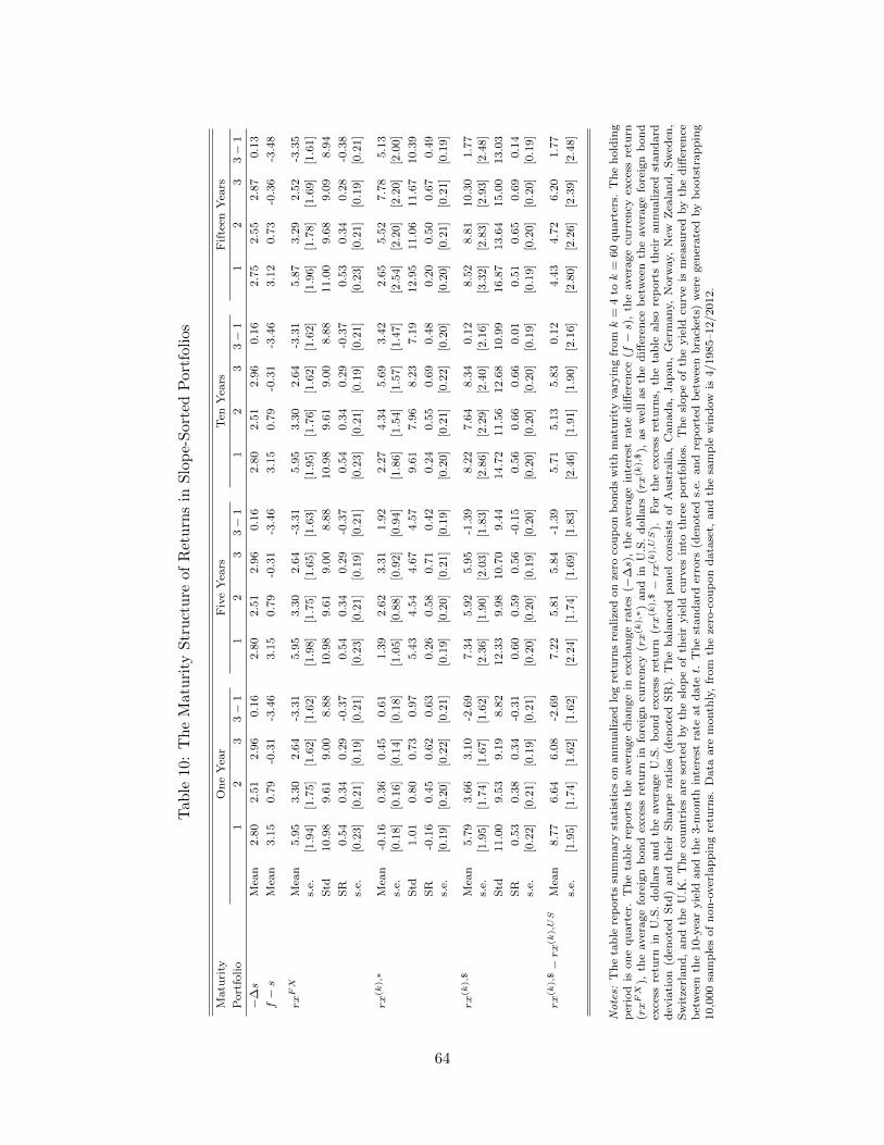
Tab

le10:

Th

eM

atu

rity

Str

uct

ure

ofR

etu

rns

inS

lop

e-S

orte

dP

ortf

olio

s

Matu

rity

On

eY

ear

Fiv

eY

ears

Ten

Yea

rsF

ifte

enY

ears

Port

folio

12

33−

11

23

3−

11

23

3−

11

23

3−

1

−∆s

Mea

n2.8

02.5

12.9

60.1

62.8

02.5

12.9

60.1

62.8

02.5

12.9

60.1

62.7

52.5

52.8

70.1

3

f−s

Mea

n3.1

50.7

9-0

.31

-3.4

63.1

50.7

9-0

.31

-3.4

63.1

50.7

9-0

.31

-3.4

63.1

20.7

3-0

.36

-3.4

8

rxFX

Mea

n5.9

53.3

02.6

4-3

.31

5.9

53.3

02.6

4-3

.31

5.9

53.3

02.6

4-3

.31

5.8

73.2

92.5

2-3

.35

s.e.

[1.9

4]

[1.7

5]

[1.6

2]

[1.6

2]

[1.9

8]

[1.7

5]

[1.6

5]

[1.6

3]

[1.9

5]

[1.7

6]

[1.6

2]

[1.6

2]

[1.9

6]

[1.7

8]

[1.6

9]

[1.6

1]

Std

10.9

89.6

19.0

08.8

810.9

89.6

19.0

08.8

810.9

89.6

19.0

08.8

811.0

09.6

89.0

98.9

4

SR

0.5

40.3

40.2

9-0

.37

0.5

40.3

40.2

9-0

.37

0.5

40.3

40.2

9-0

.37

0.5

30.3

40.2

8-0

.38

s.e.

[0.2

3]

[0.2

1]

[0.1

9]

[0.2

1]

[0.2

3]

[0.2

1]

[0.1

9]

[0.2

1]

[0.2

3]

[0.2

1]

[0.1

9]

[0.2

1]

[0.2

3]

[0.2

1]

[0.1

9]

[0.2

1]

rx

(k),∗

Mea

n-0

.16

0.3

60.4

50.6

11.3

92.6

23.3

11.9

22.2

74.3

45.6

93.4

22.6

55.5

27.7

85.1

3s.

e.[0

.18]

[0.1

6]

[0.1

4]

[0.1

8]

[1.0

5]

[0.8

8]

[0.9

2]

[0.9

4]

[1.8

6]

[1.5

4]

[1.5

7]

[1.4

7]

[2.5

4]

[2.2

0]

[2.2

0]

[2.0

0]

Std

1.0

10.8

00.7

30.9

75.4

34.5

44.6

74.5

79.6

17.9

68.2

37.1

912.9

511.0

611.6

710.3

9

SR

-0.1

60.4

50.6

20.6

30.2

60.5

80.7

10.4

20.2

40.5

50.6

90.4

80.2

00.5

00.6

70.4

9s.

e.[0

.19]

[0.2

0]

[0.2

2]

[0.2

1]

[0.1

9]

[0.2

0]

[0.2

1]

[0.1

9]

[0.2

0]

[0.2

1]

[0.2

2]

[0.2

0]

[0.2

0]

[0.2

1]

[0.2

1]

[0.1

9]

rx

(k),

$M

ean

5.7

93.6

63.1

0-2

.69

7.3

45.9

25.9

5-1

.39

8.2

27.6

48.3

40.1

28.5

28.8

110.3

01.7

7s.

e.[1

.95]

[1.7

4]

[1.6

7]

[1.6

2]

[2.3

6]

[1.9

0]

[2.0

3]

[1.8

3]

[2.8

6]

[2.2

9]

[2.4

0]

[2.1

6]

[3.3

2]

[2.8

3]

[2.9

3]

[2.4

8]

Std

11.0

09.5

39.1

98.8

212.3

39.9

810.7

09.4

414.7

211.5

612.6

810.9

916.8

713.6

415.0

013.0

3

SR

0.5

30.3

80.3

4-0

.31

0.6

00.5

90.5

6-0

.15

0.5

60.6

60.6

60.0

10.5

10.6

50.6

90.1

4s.

e.[0

.22]

[0.2

1]

[0.1

9]

[0.2

1]

[0.2

0]

[0.2

0]

[0.1

9]

[0.2

0]

[0.2

0]

[0.2

0]

[0.2

0]

[0.1

9]

[0.1

9]

[0.2

0]

[0.2

0]

[0.1

9]

rx

(k),

$−rx

(k),US

Mea

n8.7

76.6

46.0

8-2

.69

7.2

25.8

15.8

4-1

.39

5.7

15.1

35.8

30.1

24.4

34.7

26.2

01.7

7

s.e.

[1.9

5]

[1.7

4]

[1.6

2]

[1.6

2]

[2.2

4]

[1.7

4]

[1.6

9]

[1.8

3]

[2.4

6]

[1.9

1]

[1.9

0]

[2.1

6]

[2.8

0]

[2.2

6]

[2.3

9]

[2.4

8]

Notes:

Th

eta

ble

rep

ort

ssu

mm

ary

stati

stic

son

an

nu

alize

dlo

gre

turn

sre

ali

zed

on

zero

cou

pon

bon

ds

wit

hm

atu

rity

vary

ing

fromk

=4

tok

=60

qu

art

ers.

Th

eh

old

ing

per

iod

ison

equ

art

er.

Th

eta

ble

rep

ort

sth

eaver

age

chan

ge

inex

chan

ge

rate

s(−

∆s)

,th

eaver

age

inte

rest

rate

diff

eren

ce(f−s)

,th

eaver

age

curr

ency

exce

ssre

turn

(rxFX

),th

eaver

age

fore

ign

bon

dex

cess

retu

rnin

fore

ign

curr

ency

(rx

(k),∗)

an

din

U.S

.d

ollars

(rx

(k),

$),

as

wel

las

the

diff

eren

ceb

etw

een

the

aver

age

fore

ign

bon

dex

cess

retu

rnin

U.S

.d

ollars

an

dth

eaver

age

U.S

.b

on

dex

cess

retu

rn(rx

(k),

$−rx

(k),US

).F

or

the

exce

ssre

turn

s,th

eta

ble

als

ore

port

sth

eir

an

nu

alize

dst

an

dard

dev

iati

on

(den

ote

dS

td)

an

dth

eir

Sh

arp

era

tios

(den

ote

dS

R).

Th

eb

ala

nce

dp

an

elco

nsi

sts

of

Au

stra

lia,

Can

ad

a,

Jap

an

,G

erm

any,

Norw

ay,

New

Zea

lan

d,

Sw

eden

,S

wit

zerl

an

d,

an

dth

eU

.K.

Th

eco

untr

ies

are

sort

edby

the

slop

eof

thei

ryie

ldcu

rves

into

thre

ep

ort

folios.

Th

esl

op

eof

the

yie

ldcu

rve

ism

easu

red

by

the

diff

eren

ceb

etw

een

the

10-y

ear

yie

ldan

dth

e3-m

onth

inte

rest

rate

at

datet.

Th

est

an

dard

erro

rs(d

enote

ds.

e.an

dre

port

edb

etw

een

bra

cket

s)w

ere

gen

erate

dby

boots

trap

pin

g10,0

00

sam

ple

sof

non

-over

lap

pin

gre

turn

s.D

ata

are

month

ly,

from

the

zero

-cou

pon

data

set,

an

dth

esa

mp

lew

ind

ow

is4/1985–12/2012.

64

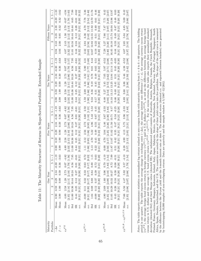
Tab

le11:

Th

eM

atu

rity

Str

uct

ure

ofR

etu

rns

inS

lop

e-S

orte

dP

ortf

olio

s:E

xte

nd

edS

am

ple

Matu

rity

On

eY

ear

Fiv

eY

ears

Ten

Yea

rsF

ifte

enY

ears

Port

folio

12

34

55−

11

23

45

5−

11

23

45

5−

11

23

45

5−

1

−∆s

Mea

n0.9

00.5

90.2

92.3

4-0

.30

-1.1

90.9

00.5

90.2

92.3

4-0

.30

-1.1

90.9

00.5

90.2

92.3

4-0

.30

-1.1

90.9

40.4

30.3

52.3

8-0

.39

-1.3

3

f−s

Mea

n3.9

91.9

90.9

90.3

90.3

6-3

.63

3.9

91.9

90.9

90.3

90.3

6-3

.63

3.9

91.9

90.9

90.3

90.3

6-3

.63

3.9

32.0

00.9

50.3

20.3

2-3

.62

rxFX

Mea

n4.8

92.5

81.2

82.7

30.0

7-4

.82

4.8

92.5

81.2

82.7

30.0

7-4

.82

4.8

92.5

81.2

82.7

30.0

7-4

.82

4.8

72.4

31.3

02.7

0-0

.07

-4.9

4s.

e.[2

.35]

[2.1

4]

[2.1

1]

[2.1

0]

[1.7

9]

[1.5

6]

[2.3

3]

[2.1

5]

[2.1

0]

[2.0

6]

[1.8

0]

[1.5

6]

[2.3

3]

[2.1

5]

[2.1

1]

[2.0

6]

[1.7

9]

[1.5

7]

[2.3

2]

[2.1

3]

[2.1

2]

[2.1

3]

[1.7

8]

[1.6

3]

Std

11.0

010.3

610.4

410.2

48.5

67.9

511.0

010.3

610.4

410.2

48.5

67.9

511.0

010.3

610.4

410.2

48.5

67.9

511.0

110.3

410.4

410.4

48.6

57.9

9

SR

0.4

40.2

50.1

20.2

70.0

1-0

.61

0.4

40.2

50.1

20.2

70.0

1-0

.61

0.4

40.2

50.1

20.2

70.0

1-0

.61

0.4

40.2

40.1

20.2

6-0

.01

-0.6

2s.

e.[0

.21]

[0.2

1]

[0.2

1]

[0.2

0]

[0.2

0]

[0.2

1]

[0.2

2]

[0.2

1]

[0.2

1]

[0.2

1]

[0.2

0]

[0.2

1]

[0.2

1]

[0.2

1]

[0.2

1]

[0.2

0]

[0.2

0]

[0.2

2]

[0.2

2]

[0.2

1]

[0.2

1]

[0.2

1]

[0.2

0]

[0.2

2]

rx

(k),∗

Mea

n-0

.09

0.1

10.3

20.3

30.6

30.7

21.1

12.1

22.5

62.7

33.6

02.5

01.5

92.6

94.1

64.3

25.9

04.3

12.4

22.8

46.3

64.7

87.7

85.3

6s.

e.[0

.21]

[0.2

0]

[0.1

7]

[0.1

7]

[0.1

7]

[0.2

3]

[1.0

8]

[0.9

5]

[1.0

6]

[0.9

5]

[1.1

0]

[1.2

1]

[1.9

0]

[1.6

6]

[1.8

6]

[1.6

1]

[1.7

7]

[1.6

9]

[2.6

3]

[2.5

6]

[2.4

2]

[2.1

2]

[2.5

4]

[2.4

0]

Std

1.0

40.8

80.8

80.8

40.8

81.1

55.1

34.7

05.2

24.9

65.4

25.5

39.3

48.5

69.1

98.7

89.0

18.4

412.6

712.8

212.5

511.9

212.7

011.7

6

SR

-0.0

90.1

20.3

70.3

90.7

20.6

30.2

20.4

50.4

90.5

50.6

70.4

50.1

70.3

10.4

50.4

90.6

50.5

10.1

90.2

20.5

10.4

00.6

10.4

6s.

e.[0

.20]

[0.2

0]

[0.2

0]

[0.2

1]

[0.2

1]

[0.2

0]

[0.2

1]

[0.2

0]

[0.2

3]

[0.2

1]

[0.2

1]

[0.2

0]

[0.2

0]

[0.2

0]

[0.2

3]

[0.2

1]

[0.2

2]

[0.2

0]

[0.2

0]

[0.2

0]

[0.2

1]

[0.2

2]

[0.2

1]

[0.2

0]

rx

(k),

$M

ean

4.8

02.6

91.6

03.0

60.7

0-4

.10

6.0

04.7

03.8

45.4

63.6

7-2

.33

6.4

85.2

75.4

57.0

55.9

7-0

.52

7.2

95.2

77.6

67.4

77.7

10.4

2s.

e.[2

.35]

[2.1

0]

[2.0

9]

[2.1

0]

[1.8

3]

[1.5

4]

[2.5

0]

[2.1

7]

[2.2

5]

[2.2

6]

[2.3

0]

[1.8

3]

[2.9

3]

[2.5

4]

[2.7

2]

[2.6

2]

[2.7

1]

[2.0

8]

[3.4

0]

[3.2

0]

[3.1

1]

[2.9

7]

[3.2

9]

[2.6

7]

Std

11.0

510.2

910.3

210.2

78.7

27.9

911.8

711.0

711.0

211.5

010.7

19.1

714.1

013.1

313.2

513.8

413.1

411.2

416.4

516.1

015.7

416.0

415.9

613.9

7

SR

0.4

30.2

60.1

60.3

00.0

8-0

.51

0.5

10.4

20.3

50.4

70.3

4-0

.25

0.4

60.4

00.4

10.5

10.4

5-0

.05

0.4

40.3

30.4

90.4

70.4

80.0

3s.

e.[0

.21]

[0.2

1]

[0.2

1]

[0.2

0]

[0.2

0]

[0.2

1]

[0.2

0]

[0.2

1]

[0.2

1]

[0.2

1]

[0.2

1]

[0.2

0]

[0.2

0]

[0.2

1]

[0.2

1]

[0.2

1]

[0.2

0]

[0.2

0]

[0.2

1]

[0.2

1]

[0.2

1]

[0.2

1]

[0.2

0]

[0.2

0]

rx

(k),

$−rx

(k),US

Mea

n7.6

65.5

64.4

75.9

23.5

7-4

.10

6.2

84.9

94.1

35.7

53.9

6-2

.33

4.8

93.6

83.8

65.4

64.3

8-0

.52

4.6

72.6

55.0

44.8

55.0

90.4

2s.

e.[2

.35]

[2.0

8]

[2.0

7]

[2.0

8]

[1.7

9]

[1.5

4]

[2.5

7]

[2.1

3]

[2.0

5]

[2.2

1]

[2.1

3]

[1.8

3]

[2.9

5]

[2.4

1]

[2.3

8]

[2.5

9]

[2.4

2]

[2.0

8]

[3.3

7]

[3.1

0]

[2.7

8]

[2.9

7]

[3.0

0]

[2.6

7]

Notes:

Th

eta

ble

rep

ort

ssu

mm

ary

stati

stic

son

an

nu

alize

dlo

gre

turn

sre

ali

zed

on

zero

cou

pon

bon

ds

wit

hm

atu

rity

vary

ing

fromk

=4

tok

=60

qu

art

ers.

Th

eh

old

ing

per

iod

ison

equ

art

er.

Th

eta

ble

rep

ort

sth

eaver

age

chan

ge

inex

chan

ge

rate

s(−

∆s)

,th

eaver

age

inte

rest

rate

diff

eren

ce(f−s)

,th

eaver

age

curr

ency

exce

ssre

turn

(rxFX

),th

eaver

age

fore

ign

bon

dex

cess

retu

rnin

fore

ign

curr

ency

(rx

(k),∗)

an

din

U.S

.d

ollars

(rx

(k),

$),

as

wel

las

the

diff

eren

ceb

etw

een

the

aver

age

fore

ign

bon

dex

cess

retu

rnin

U.S

.d

ollars

an

dth

eaver

age

U.S

.b

on

dex

cess

retu

rn(rx

(k),

$−rx

(k),US

).F

or

the

exce

ssre

turn

s,th

eta

ble

als

ore

port

sth

eir

an

nu

alize

dst

an

dard

dev

iati

on

(den

ote

dS

td)

an

dth

eir

Sh

arp

era

tios

(den

ote

dS

R).

Th

eu

nb

ala

nce

dp

an

elco

nsi

sts

of

Au

stra

lia,

Au

stri

a,

Bel

giu

m,

Can

ad

a,

the

Cze

chR

epu

blic,

Den

mark

,F

inla

nd

,F

ran

ce,

Ger

many,

Hu

ngary

,In

don

esia

,Ir

elan

d,

Italy

,Jap

an

,M

ala

ysi

a,

Mex

ico,

the

Net

her

lan

ds,

New

Zea

lan

d,

Norw

ay,

Pola

nd

,P

ort

ugal,

Sin

gap

ore

,S

ou

thA

fric

a,

Sp

ain

,S

wed

en,

Sw

itze

rlan

d,

an

dth

eU

.K.

Th

eco

untr

ies

are

sort

edby

the

slop

eof

thei

ryie

ldcu

rves

into

five

port

folios.

Th

esl

op

eof

the

yie

ldcu

rve

ism

easu

red

by

the

diff

eren

ceb

etw

een

the

10-y

ear

yie

ldan

dth

e3-m

onth

inte

rest

rate

at

datet.

Th

est

an

dard

erro

rs(d

enote

ds.

e.an

dre

port

edb

etw

een

bra

cket

s)w

ere

gen

erate

dby

boots

trap

pin

g10,0

00

sam

ple

sof

non

-over

lap

pin

gre

turn

s.D

ata

are

qu

art

erly

an

dth

esa

mp

lew

ind

ow

is5/1987–12/2012.

65

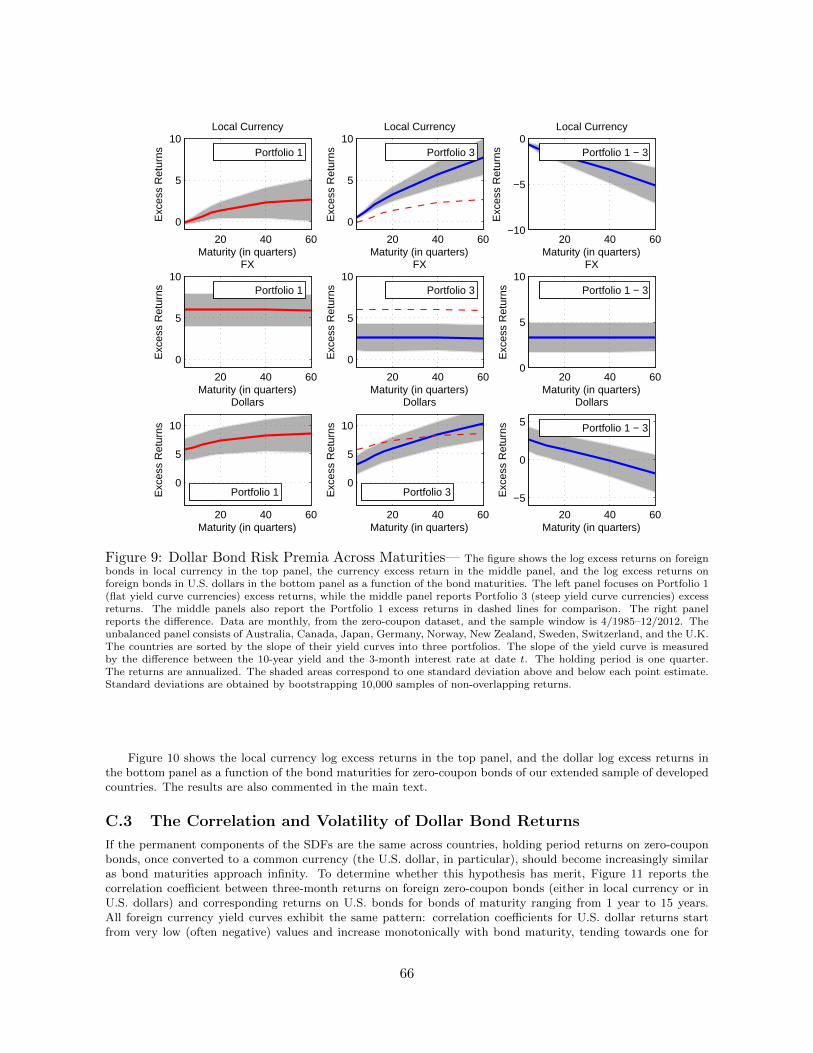
Exc

ess

Ret

urns

Maturity (in quarters)

Local Currency

20 40 60

0

5

10Portfolio 1

Exc

ess

Ret

urns

Maturity (in quarters)

Local Currency

20 40 60

0

5

10Portfolio 3

Exc

ess

Ret

urns

Maturity (in quarters)

Local Currency

20 40 60−10

−5

0Portfolio 1 − 3

Exc

ess

Ret

urns

Maturity (in quarters)

FX

20 40 60

0

5

10Portfolio 1

Exc

ess

Ret

urns

Maturity (in quarters)

FX

20 40 60

0

5

10Portfolio 3

Exc

ess

Ret

urns

Maturity (in quarters)

FX

20 40 600

5

10Portfolio 1 − 3

Exc

ess

Ret

urns

Maturity (in quarters)

Dollars

20 40 60

0

5

10

Portfolio 1 Exc

ess

Ret

urns

Maturity (in quarters)

Dollars

20 40 60

0

5

10

Portfolio 3 Exc

ess

Ret

urns

Maturity (in quarters)

Dollars

20 40 60

−5

0

5 Portfolio 1 − 3

Figure 9: Dollar Bond Risk Premia Across Maturities— The figure shows the log excess returns on foreignbonds in local currency in the top panel, the currency excess return in the middle panel, and the log excess returns onforeign bonds in U.S. dollars in the bottom panel as a function of the bond maturities. The left panel focuses on Portfolio 1(flat yield curve currencies) excess returns, while the middle panel reports Portfolio 3 (steep yield curve currencies) excessreturns. The middle panels also report the Portfolio 1 excess returns in dashed lines for comparison. The right panelreports the difference. Data are monthly, from the zero-coupon dataset, and the sample window is 4/1985–12/2012. Theunbalanced panel consists of Australia, Canada, Japan, Germany, Norway, New Zealand, Sweden, Switzerland, and the U.K.The countries are sorted by the slope of their yield curves into three portfolios. The slope of the yield curve is measuredby the difference between the 10-year yield and the 3-month interest rate at date t. The holding period is one quarter.The returns are annualized. The shaded areas correspond to one standard deviation above and below each point estimate.Standard deviations are obtained by bootstrapping 10,000 samples of non-overlapping returns.

Figure 10 shows the local currency log excess returns in the top panel, and the dollar log excess returns inthe bottom panel as a function of the bond maturities for zero-coupon bonds of our extended sample of developedcountries. The results are also commented in the main text.

C.3 The Correlation and Volatility of Dollar Bond Returns

If the permanent components of the SDFs are the same across countries, holding period returns on zero-couponbonds, once converted to a common currency (the U.S. dollar, in particular), should become increasingly similaras bond maturities approach infinity. To determine whether this hypothesis has merit, Figure 11 reports thecorrelation coefficient between three-month returns on foreign zero-coupon bonds (either in local currency or inU.S. dollars) and corresponding returns on U.S. bonds for bonds of maturity ranging from 1 year to 15 years.All foreign currency yield curves exhibit the same pattern: correlation coefficients for U.S. dollar returns startfrom very low (often negative) values and increase monotonically with bond maturity, tending towards one for

66

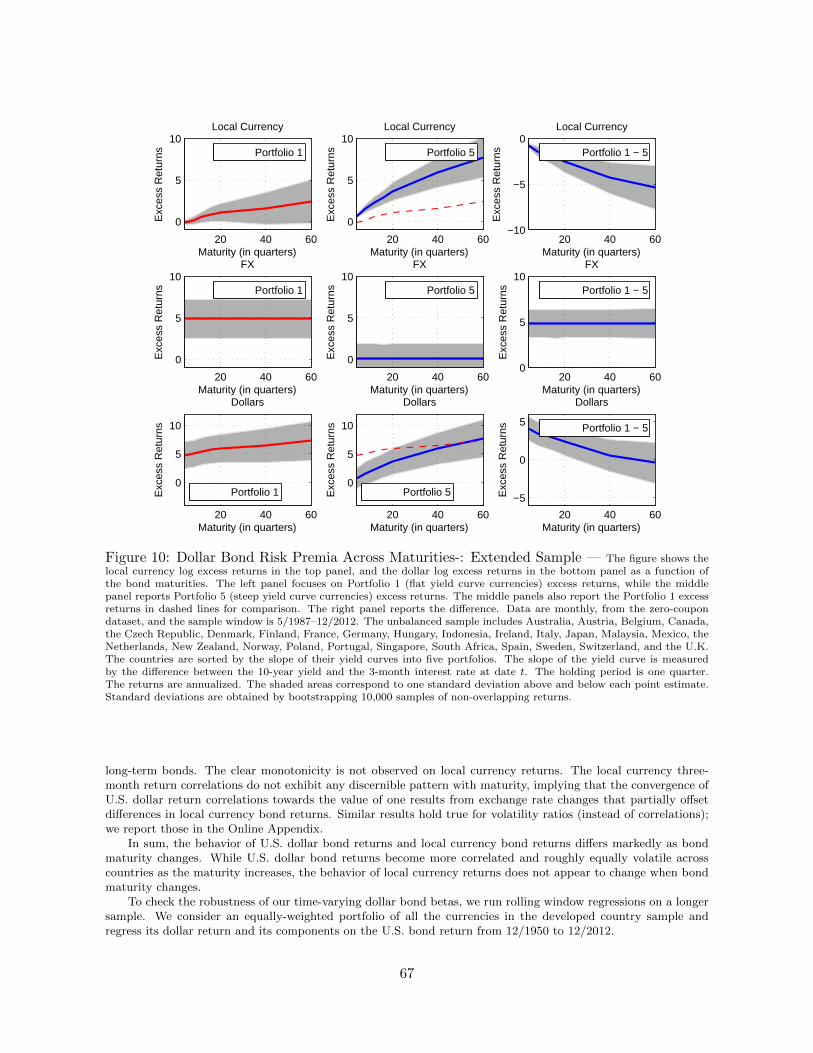
Exc

ess

Ret

urns

Maturity (in quarters)

Local Currency

20 40 60

0

5

10Portfolio 1

Exc

ess

Ret

urns

Maturity (in quarters)

Local Currency

20 40 60

0

5

10Portfolio 5

Exc

ess

Ret

urns

Maturity (in quarters)

FX

20 40 60

0

5

10Portfolio 1

Exc

ess

Ret

urns

Maturity (in quarters)

FX

20 40 60

0

5

10Portfolio 5

Exc

ess

Ret

urns

Maturity (in quarters)

Dollars

20 40 60

0

5

10

Portfolio 1 Exc

ess

Ret

urns

Maturity (in quarters)

Dollars

20 40 60

0

5

10

Portfolio 5E

xces

s R

etur

ns

Maturity (in quarters)

Local Currency

20 40 60−10

−5

0Portfolio 1 − 5

Exc

ess

Ret

urns

Maturity (in quarters)

Dollars

20 40 60

−5

0

5 Portfolio 1 − 5

Exc

ess

Ret

urns

Maturity (in quarters)

FX

20 40 600

5

10Portfolio 1 − 5

Figure 10: Dollar Bond Risk Premia Across Maturities-: Extended Sample — The figure shows thelocal currency log excess returns in the top panel, and the dollar log excess returns in the bottom panel as a function ofthe bond maturities. The left panel focuses on Portfolio 1 (flat yield curve currencies) excess returns, while the middlepanel reports Portfolio 5 (steep yield curve currencies) excess returns. The middle panels also report the Portfolio 1 excessreturns in dashed lines for comparison. The right panel reports the difference. Data are monthly, from the zero-coupondataset, and the sample window is 5/1987–12/2012. The unbalanced sample includes Australia, Austria, Belgium, Canada,the Czech Republic, Denmark, Finland, France, Germany, Hungary, Indonesia, Ireland, Italy, Japan, Malaysia, Mexico, theNetherlands, New Zealand, Norway, Poland, Portugal, Singapore, South Africa, Spain, Sweden, Switzerland, and the U.K.The countries are sorted by the slope of their yield curves into five portfolios. The slope of the yield curve is measuredby the difference between the 10-year yield and the 3-month interest rate at date t. The holding period is one quarter.The returns are annualized. The shaded areas correspond to one standard deviation above and below each point estimate.Standard deviations are obtained by bootstrapping 10,000 samples of non-overlapping returns.

long-term bonds. The clear monotonicity is not observed on local currency returns. The local currency three-month return correlations do not exhibit any discernible pattern with maturity, implying that the convergence ofU.S. dollar return correlations towards the value of one results from exchange rate changes that partially offsetdifferences in local currency bond returns. Similar results hold true for volatility ratios (instead of correlations);we report those in the Online Appendix.

In sum, the behavior of U.S. dollar bond returns and local currency bond returns differs markedly as bondmaturity changes. While U.S. dollar bond returns become more correlated and roughly equally volatile acrosscountries as the maturity increases, the behavior of local currency returns does not appear to change when bondmaturity changes.

To check the robustness of our time-varying dollar bond betas, we run rolling window regressions on a longersample. We consider an equally-weighted portfolio of all the currencies in the developed country sample andregress its dollar return and its components on the U.S. bond return from 12/1950 to 12/2012.

67

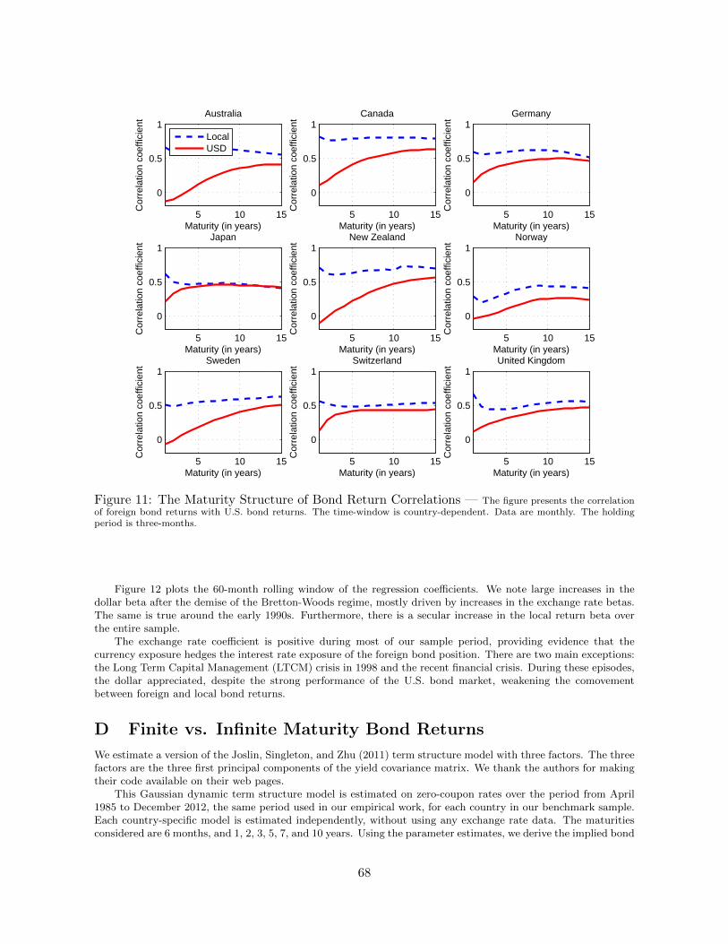
5 10 15

0

0.5

1Australia

Maturity (in years)

Cor

rela

tion

coef

ficie

nt

LocalUSD

5 10 15

0

0.5

1Canada

Maturity (in years)

Cor

rela

tion

coef

ficie

nt

5 10 15

0

0.5

1Germany

Maturity (in years)

Cor

rela

tion

coef

ficie

nt

5 10 15

0

0.5

1Japan

Maturity (in years)

Cor

rela

tion

coef

ficie

nt

5 10 15

0

0.5

1New Zealand

Maturity (in years)

Cor

rela

tion

coef

ficie

nt

5 10 15

0

0.5

1Norway

Maturity (in years)

Cor

rela

tion

coef

ficie

nt5 10 15

0

0.5

1Sweden

Maturity (in years)

Cor

rela

tion

coef

ficie

nt

5 10 15

0

0.5

1Switzerland

Maturity (in years)

Cor

rela

tion

coef

ficie

nt

5 10 15

0

0.5

1United Kingdom

Maturity (in years)

Cor

rela

tion

coef

ficie

nt

Figure 11: The Maturity Structure of Bond Return Correlations — The figure presents the correlationof foreign bond returns with U.S. bond returns. The time-window is country-dependent. Data are monthly. The holdingperiod is three-months.

Figure 12 plots the 60-month rolling window of the regression coefficients. We note large increases in thedollar beta after the demise of the Bretton-Woods regime, mostly driven by increases in the exchange rate betas.The same is true around the early 1990s. Furthermore, there is a secular increase in the local return beta overthe entire sample.

The exchange rate coefficient is positive during most of our sample period, providing evidence that thecurrency exposure hedges the interest rate exposure of the foreign bond position. There are two main exceptions:the Long Term Capital Management (LTCM) crisis in 1998 and the recent financial crisis. During these episodes,the dollar appreciated, despite the strong performance of the U.S. bond market, weakening the comovementbetween foreign and local bond returns.

D Finite vs. Infinite Maturity Bond Returns

We estimate a version of the Joslin, Singleton, and Zhu (2011) term structure model with three factors. The threefactors are the three first principal components of the yield covariance matrix. We thank the authors for makingtheir code available on their web pages.

This Gaussian dynamic term structure model is estimated on zero-coupon rates over the period from April1985 to December 2012, the same period used in our empirical work, for each country in our benchmark sample.Each country-specific model is estimated independently, without using any exchange rate data. The maturitiesconsidered are 6 months, and 1, 2, 3, 5, 7, and 10 years. Using the parameter estimates, we derive the implied bond

68

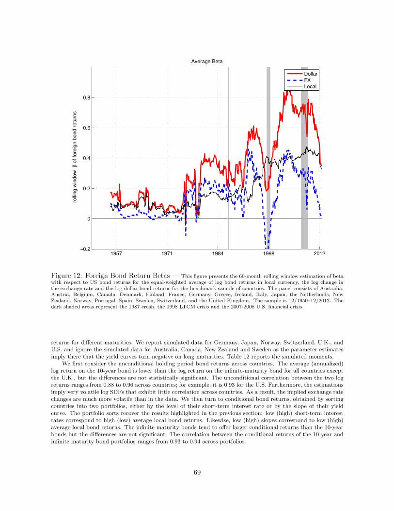
1957 1971 1984 1998 2012−0.2

0

0.2

0.4

0.6

0.8

rolli

ng w

indow

β o

f fo

reig

n b

ond r

etu

rns

Average Beta

Dollar

FX

Local

Figure 12: Foreign Bond Return Betas — This figure presents the 60-month rolling window estimation of betawith respect to US bond returns for the equal-weighted average of log bond returns in local currency, the log change inthe exchange rate and the log dollar bond returns for the benchmark sample of countries. The panel consists of Australia,Austria, Belgium, Canada, Denmark, Finland, France, Germany, Greece, Ireland, Italy, Japan, the Netherlands, NewZealand, Norway, Portugal, Spain, Sweden, Switzerland, and the United Kingdom. The sample is 12/1950–12/2012. Thedark shaded areas represent the 1987 crash, the 1998 LTCM crisis and the 2007-2008 U.S. financial crisis.

returns for different maturities. We report simulated data for Germany, Japan, Norway, Switzerland, U.K., andU.S. and ignore the simulated data for Australia, Canada, New Zealand and Sweden as the parameter estimatesimply there that the yield curves turn negative on long maturities. Table 12 reports the simulated moments.

We first consider the unconditional holding period bond returns across countries. The average (annualized)log return on the 10-year bond is lower than the log return on the infinite-maturity bond for all countries exceptthe U.K., but the differences are not statistically significant. The unconditional correlation between the two logreturns ranges from 0.88 to 0.96 across countries; for example, it is 0.93 for the U.S. Furthermore, the estimationsimply very volatile log SDFs that exhibit little correlation across countries. As a result, the implied exchange ratechanges are much more volatile than in the data. We then turn to conditional bond returns, obtained by sortingcountries into two portfolios, either by the level of their short-term interest rate or by the slope of their yieldcurve. The portfolio sorts recover the results highlighted in the previous section: low (high) short-term interestrates correspond to high (low) average local bond returns. Likewise, low (high) slopes correspond to low (high)average local bond returns. The infinite maturity bonds tend to offer larger conditional returns than the 10-yearbonds but the differences are not significant. The correlation between the conditional returns of the 10-year andinfinite maturity bond portfolios ranges from 0.93 to 0.94 across portfolios.

69

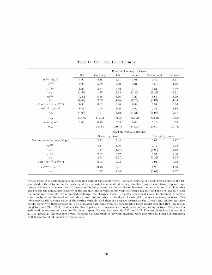
Table 12: Simulated Bond Returns

Panel A: Country Returns

US Germany UK Japan Switzerland Norway

y(10) (data) 5.92 5.38 6.51 3.01 3.49 4.67

y(10) 5.93 5.38 6.50 3.01 3.50 4.68

rx(10) 6.06 4.21 3.63 4.18 2.84 3.07s.e. [1.52] [1.25] [1.63] [1.26] [1.22] [1.91]

rx(∞) 12.54 5.76 3.36 7.20 5.67 5.90s.e. [5.44] [2.58] [4.45] [2.75] [3.01] [4.34]

Corr (rx(10), rx(∞)) 0.93 0.92 0.88 0.94 0.94 0.96

rx(∞) − rx(10) 6.47 1.55 -0.27 3.02 2.83 2.84

s.e. [4.05] [1.51] [3.12] [1.61] [1.93] [2.57]

σm? 245.55 112.44 156.56 206.23 226.16 128.55

corr(m,m?) 1.00 0.19 0.03 0.03 0.13 0.03

σ∆s 249.80 286.73 315.23 279.01 207.43

Panel B: Portfolio Returns

Sorted by Level Sorted by Slope

Sorting variable (level/slope) 2.42 5.44 0.07 1.87

rx(10) 4.47 3.96 2.72 5.34

s.e. [1.17] [1.27] [1.26] [1.18]

rx(∞) 7.62 6.27 3.97 9.40s.e. [2.93] [3.37] [3.22] [3.35]

Corr (rx(10), rx(∞)) 0.93 0.93 0.94 0.93

rx(∞) − rx(10) 3.16 2.31 1.26 4.06

s.e. [1.87] [2.24] [2.04] [2.27]

Notes: Panel A reports moments on simulated data at the country level. For each country, the table first compares the 10-year yield in the data and in the model, and then reports the annualized average simulated log excess return (in percentageterms) of bonds with maturities of 10 years and infinity, as well as the correlation between the two bond returns. The tablealso reports the annualized volatility of the log SDF, the correlation between the foreign log SDF and the U.S. log SDF, andthe annualized volatility of the implied exchange rate changes. Panel B reports conditional moments obtained by sortingcountries by either the level of their short-term interest rates or the slope of their yield curves into two portfolios. Thetable reports the average value of the sorting variable, and then the average returns on the 10-year and infinite-maturitybonds, along with their correlation. The simulated data come from the benchmark 3-factor model (denoted RPC) in Joslin,Singleton, and Zhu (2011) that sets the first 3 principal components of bond yields as the pricing factors. The model isestimated on zero-coupon rates for Germany, Japan, Norway, Switzerland, U.K., and U.S. The sample estimation period is4/1985–12/2012. The standard errors (denoted s.e. and reported between brackets) were generated by block-bootstrapping10,000 samples of 333 monthly observations.

70

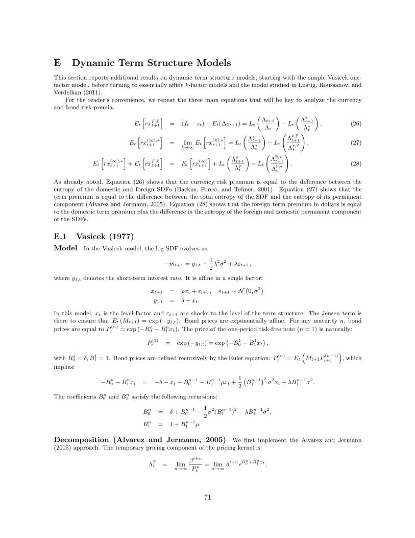
E Dynamic Term Structure Models

This section reports additional results on dynamic term structure models, starting with the simple Vasicek one-factor model, before turning to essentially affine k-factor models and the model studied in Lustig, Roussanov, andVerdelhan (2011).

For the reader’s convenience, we repeat the three main equations that will be key to analyze the currencyand bond risk premia:

Et[rxFXt+1

]= (ft − st)− Et(∆st+1) = Lt

(Λt+1

Λt

)− Lt

(Λ∗t+1

Λ∗t

), (26)

Et[rx

(∞),∗t+1

]= lim

k→∞Et[rx

(k),∗t+1

]= Lt

(Λ∗t+1

Λ∗t

)− Lt

(Λ∗,Pt+1

Λ∗,Pt

), (27)

Et[rx

(∞),∗t+1

]+ Et

[rxFXt+1

]= Et

[rx

(∞)t+1

]+ Lt

(ΛPt+1

ΛPt

)− Lt

(ΛP,∗t+1

ΛP,∗t

). (28)

As already noted, Equation (26) shows that the currency risk premium is equal to the difference between theentropy of the domestic and foreign SDFs (Backus, Foresi, and Telmer, 2001). Equation (27) shows that theterm premium is equal to the difference between the total entropy of the SDF and the entropy of its permanentcomponent (Alvarez and Jermann, 2005). Equation (28) shows that the foreign term premium in dollars is equalto the domestic term premium plus the difference in the entropy of the foreign and domestic permanent componentof the SDFs.

E.1 Vasicek (1977)

Model In the Vasicek model, the log SDF evolves as:

−mt+1 = y1,t +1

2λ2σ2 + λεt+1,

where y1,t denotes the short-term interest rate. It is affine in a single factor:

xt+1 = ρxt + εt+1, εt+1 ∼ N(0, σ2)

y1,t = δ + xt.

In this model, xt is the level factor and εt+1 are shocks to the level of the term structure. The Jensen term isthere to ensure that Et (Mt+1) = exp (−y1,t). Bond prices are exponentially affine. For any maturity n, bond

prices are equal to P(n)t = exp (−Bn0 −Bn1 xt). The price of the one-period risk-free note (n = 1) is naturally:

P(1)t = exp (−y1,t) = exp

(−B1

0 −B11xt),

with B10 = δ,B1

1 = 1. Bond prices are defined recursively by the Euler equation: P(n)t = Et

(Mt+1P

(n−1)t+1

), which

implies:

−Bn0 −Bn1 xt = −δ − xt −Bn−10 −Bn−1

1 ρxt +1

2

(Bn−1

1

)2σ2xt + λBn−1

1 σ2.

The coefficients Bn0 and Bn1 satisfy the following recursions:

Bn0 = δ +Bn−10 − 1

2σ2(Bn−1

1 )2 − λBn−11 σ2,

Bn1 = 1 +Bn−11 ρ.

Decomposition (Alvarez and Jermann, 2005) We first implement the Alvarez and Jermann(2005) approach. The temporary pricing component of the pricing kernel is:

ΛTt = lim

n→∞

βt+n

Pnt= limn→∞

βt+neBn0 +Bn1 xt ,

71

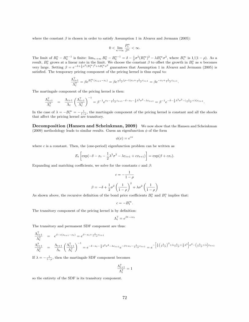
where the constant β is chosen in order to satisfy Assumption 1 in Alvarez and Jermann (2005):

0 < limn→∞

Pntβn

<∞.

The limit of Bn0 − Bn−10 is finite: limn→∞B

n0 − Bn−1

0 = δ − 12σ2(B∞1 )2 − λB∞1 σ2, where B∞1 is 1/(1− ρ). As a

result, Bn0 grows at a linear rate in the limit. We choose the constant β to offset the growth in Bn0 as n becomes

very large. Setting β = e−δ+12σ2(B∞1 )2+λB∞1 σ2

guarantees that Assumption 1 in Alvarez and Jermann (2005) issatisfied. The temporary pricing component of the pricing kernel is thus equal to:

ΛTt+1

ΛTt

= βeB∞1 (xt+1−xt) = βe

11−ρ (ρ−1)xt+

11−ρ εt+1 = βe

−xt+ 11−ρ εt+1 .

The martingale component of the pricing kernel is then:

ΛPt+1

ΛPt

=Λt+1

Λt

(ΛTt+1

ΛTt

)−1

= β−1ext− 1

1−ρ εt+1−δ−xt− 12λ2σ2−λεt+1 = β−1e

−δ− 12λ2σ2−( 1

1−ρ+λ)εt+1 .

In the case of λ = −B∞1 = − 11−ρ , the martingale component of the pricing kernel is constant and all the shocks

that affect the pricing kernel are transitory.

Decomposition (Hansen and Scheinkman, 2009) We now show that the Hansen and Scheinkman(2009) methodology leads to similar results. Guess an eigenfunction φ of the form

φ(x) = ecx

where c is a constant. Then, the (one-period) eigenfunction problem can be written as

Et

[exp(−δ − xt −

1

2λ2σ2 − λεt+1 + cxt+1)

]= exp(β + cxt).

Expanding and matching coefficients, we solve for the constants c and β:

c = − 1

1− ρ

β = −δ +1

2σ2

(1

1− ρ

)2

+ λσ2

(1

1− ρ

)As shown above, the recursive definition of the bond price coefficients Bn0 and Bn1 implies that:

c = −B∞1 .

The transitory component of the pricing kernel is by definition:

ΛTt = eβt−cxt

The transitory and permanent SDF component are thus:

ΛTt+1

ΛTt

= eβ−c(xt+1−xt) = eβ−xt+ 1

1−ρ εt+1

ΛPt+1

ΛPt

=Λt+1

Λt

(ΛTt+1

ΛTt

)−1

= e−δ−xt−12λ2σ2−λεt+1e

−β+xt− 11−ρ εt+1 = e

−[12

(1

1−ρ

)2+λ 1

1−ρ+ 12λ2]σ2−

(1

1−ρ+λ)εt+1

If λ = − 11−ρ , then the martingale SDF component becomes

ΛPt+1

ΛPt

= 1

so the entirety of the SDF is its transitory component.

72

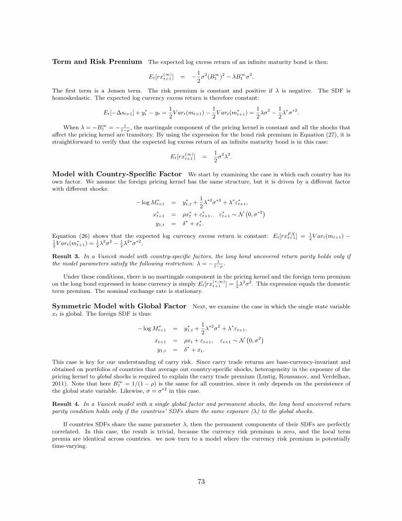
Term and Risk Premium The expected log excess return of an infinite maturity bond is then:

Et[rx(∞)t+1 ] = −1

2σ2(B∞1 )2 − λB∞1 σ2.

The first term is a Jensen term. The risk premium is constant and positive if λ is negative. The SDF ishomoskedastic. The expected log currency excess return is therefore constant:

Et[−∆st+1] + y∗t − yt =1

2V art(mt+1)− 1

2V art(m

∗t+1) =

1

2λσ2 − 1

2λ∗σ∗2.

When λ = −B∞1 = − 11−ρ , the martingale component of the pricing kernel is constant and all the shocks that

affect the pricing kernel are transitory. By using the expression for the bond risk premium in Equation (27), it isstraightforward to verify that the expected log excess return of an infinite maturity bond is in this case:

Et[rx(∞)t+1 ] =

1

2σ2λ2.

Model with Country-Specific Factor We start by examining the case in which each country has itsown factor. We assume the foreign pricing kernel has the same structure, but it is driven by a different factorwith different shocks:

− logM∗t+1 = y∗1,t +1

2λ∗2σ∗2 + λ∗ε∗t+1,

x∗t+1 = ρx∗t + ε∗t+1, ε∗t+1 ∼ N(0, σ∗2

)y1,t = δ∗ + x∗t .

Equation (26) shows that the expected log currency excess return is constant: Et[rxFXt+1] = 1

2V art(mt+1) −

12V art(m

∗t+1) = 1

2λ2σ2 − 1

2λ2∗σ∗2.

Result 3. In a Vasicek model with country-specific factors, the long bond uncovered return parity holds only ifthe model parameters satisfy the following restriction: λ = − 1

1−ρ .

Under these conditions, there is no martingale component in the pricing kernel and the foreign term premiumon the long bond expressed in home currency is simply Et[rx

(∗,∞)t+1 ] = 1

2λ2σ2. This expression equals the domestic

term premium. The nominal exchange rate is stationary.

Symmetric Model with Global Factor Next, we examine the case in which the single state variablext is global. The foreign SDF is thus:

− logM∗t+1 = y∗1,t +1

2λ∗2σ2 + λ∗εt+1,

xt+1 = ρxt + εt+1, εt+1 ∼ N(0, σ2)

y1,t = δ∗ + xt.

This case is key for our understanding of carry risk. Since carry trade returns are base-currency-invariant andobtained on portfolios of countries that average out country-specific shocks, heterogeneity in the exposure of thepricing kernel to global shocks is required to explain the carry trade premium (Lustig, Roussanov, and Verdelhan,2011). Note that here B∞1 = 1/(1 − ρ) is the same for all countries, since it only depends on the persistence ofthe global state variable. Likewise, σ = σ∗2 in this case.

Result 4. In a Vasicek model with a single global factor and permanent shocks, the long bond uncovered returnparity condition holds only if the countries’ SDFs share the same exposure (λ) to the global shocks.

If countries SDFs share the same parameter λ, then the permanent components of their SDFs are perfectlycorrelated. In this case, the result is trivial, because the currency risk premium is zero, and the local termpremia are identical across countries. we now turn to a model where the currency risk premium is potentiallytime-varying.

73

E.2 Cox, Ingersoll, and Ross (1985) Model

Model The Cox, Ingersoll, and Ross (1985) model (denoted CIR) is defined by the following two equations:

− logMt+1 = α+ χzt +√γztut+1, (29)

zt+1 = (1− φ)θ + φzt − σ√ztut+1,

where M denotes the stochastic discount factor. In this model, log bond prices are affine in the state variable z:

p(n)t = −Bn0 −Bn1 zt. The price of a one period-bond is: P (1) = Et(Mt+1) = e−α−(χ− 1

2γ)zt . Bond prices are defined

recursively by the Euler equation: P(n)t = Et(Mt+1P

(n−1)t+1 ). Thus the bond price coefficients evolve according to

the following second-order difference equations:

Bn0 = α+Bn−10 +Bn−1

1 (1− φ)θ, (30)

Bn1 = χ− 1

2γ +Bn−1

1 φ− 1

2

(Bn−1

1

)2σ2 + σ

√γBn−1

1 .

Decomposition (Alvarez and Jermann, 2005) We first implement the Alvarez and Jermann(2005) approach. The temporary pricing component of the pricing kernel is:

ΛTt = lim

n→∞

βt+n

P(n)t

= limn→∞

βt+neBn0 +Bn1 zt ,

where the constant β is chosen in order to satisfy Assumption 1 in Alvarez and Jermann (2005):

0 < limn→∞

P(n)t

βn<∞.

The limit of Bn0 − Bn−10 is finite: limn→∞B

n0 − Bn−1

0 = α + B∞1 (1 − φ)θ, where B∞1 is defined implicitly in asecond-order equation above. As a result, Bn0 grows at a linear rate in the limit. We choose the constant β tooffset the growth in Bn0 as n becomes very large. Setting β = e−α−B

∞1 (1−φ)θ guarantees that Assumption 1 in

Alvarez and Jermann (2005) is satisfied. The temporary pricing component of the SDF is thus equal to:

ΛTt+1

ΛTt

= βeB∞1 (zt+1−zt) = βeB

∞1 [(φ−1)(zt−θ)−σ

√ztut+1].

As a result, the martingale component of the SDF is then:

ΛPt+1

ΛPt

=Λt+1

Λt

(ΛTt+1

ΛTt

)−1

= β−1e−α−χzt−√γztut+1e−B

∞1 [(φ−1)(zt−θ)−σ

√ztut+1]. (31)

Decomposition (Hansen and Scheinkman, 2009) We now show that the Hansen and Scheinkman(2009) methodology leads to similar results. We guess an eigenfunction φ of the form

φ(x) = ecz

where c is a constant. Then, the (one-period) eigenfunction problem can be written as

Et [exp(α+ χzt +√γztut+1 + czt+1)] = exp(β + czt).

Expanding and matching coefficients, we get:

β = −α+ c(1− φ)θ[1

2σ2

]c2 + [σ

√γ + φ− 1] c+

[1

2γ − χ

]= 0

so c solves a quadratic equation. The transitory component of the pricing kernel is by definition:

ΛTt = eβt−czt

74

The transitory and permanent SDF component are thus:

ΛTt+1

ΛTt

= eβ−c(zt+1−zt) = eβ−c[(1−φ)(θ−zt)−σ√ztut+1] = e−α+c[(1−φ)zt+σ

√ztut+1]

ΛPt+1

ΛPt

=Λt+1

Λt

(ΛTt+1

ΛTt

)−1

= e−α−χzt−√γztut+1eα−c[(1−φ)zt+σ

√ztut+1] = e−[χ+c(1−φ)]zt−[√γ+cσ]

√ztut+1

The law of motion of bond prices implies that c = −B∞1 . If χ = −c(1 − φ), then the quadratic equation for cbecomes

σ2c2 + 2σ√γc+ γ = 0

with unique solution c = −√γ

σ. Then, the martingale component of the SDF becomes

ΛPt+1

ΛPt

= 1

so the entirety of the SDF is its transitory component.

Term Premium The expected log excess return is thus given by:

Et[rx(n)t+1] = [−1

2

(Bn−1

1

)2σ2 + σ

√γBn−1

1 ]zt.

The expected log excess return of an infinite maturity bond is then:

Et[rx(∞)t+1 ] = [−1

2(B∞1 )2 σ2 + σ

√γB∞1 ]zt,

= [B∞1 (1− φ)− χ+1

2γ]zt.

The − 12

(B∞1 )2 σ2 is a Jensen term. The term premium is driven by σ√γB∞1 zt, where B∞1 is defined implicitly

in the second order equation B∞1 = χ− 12γ +B∞1 φ− 1

2(B∞1 )2 σ2 + σ

√γB∞1 .

Model with Country-specific Factors Consider the special case of B∞1 (1−φ) = χ. In this case, the

expected term premium is simply Et[rx(∞)t+1 ] = 1

2γzt, which is equal to one-half of the variance of the log stochastic

discount factor.Suppose that the foreign pricing kernel is specified as in Equation (35) with the same parameters. However,the foreign country has its own factor z∗. As a result, the difference between the domestic and foreign log termpremia is equal to the log currency risk premium, which is given by Et[rx

FXt+1] = 1

2γ(zt − z∗t ). In other words, the

expected foreign log holding period return on a foreign long bond converted into U.S. dollars is equal to the U.S.term premium: Et[rx

(∞),∗t+1 ] + Et[rx

FXt+1] = 1

2γzt.

This special case corresponds to the absence of permanent shocks to the SDF: when B∞1 (1−φ) = χ, the permanentcomponent of the stochastic discount factor is constant. To see this result, let us go back to the implicit definitionof B∞1 in Equation (31):

0 =1

2(B∞1 )2 σ2 + (1− φ− σ√γ)B∞1 − χ+

1

2γ,

0 =1

2(B∞1 )2 σ2 − σ√γB∞1 +

1

2γ,

0 = (σB∞1 −√γ)2 .

In this special case, B∞1 =√γ/σ. Using this result in Equation (31), the permanent component of the SDF

reduces to:

MPt+1

MPt

=Mt+1

Mt

(MTt+1

MTt

)−1

= β−1e−α−χzt−√γztut+1e−B

∞1 [(φ−1)(zt−θ)−σ

√ztut+1] = β−1e−α−χθ,

which is a constant.

75

Model with Global Factors We assume that all the shocks are global and that zt is a global statevariable (and thus σ = σ∗, φ = φ∗, θ = θ∗). The state variable is referred as “permanent” if it has some impacton the permanent component of the SDF. The difference in term premia between the domestic and foreign bond(once expressed in the same currency) is pinned down by the difference in conditional variances of the permanentcomponents of the SDFs. Therefore the two bonds have the same risk premia when:

√γ +B∞1 σ =

√γ∗ +B∞∗1 σ

Note that B∞1 depends on χ and γ, as well as on the global parameters φ and σ. The domestic and foreign infinite-maturity bonds have the same risk premia (once expressed in the same currency) when γ = γ∗ and χ = χ∗, i.e.when the domestic and foreign SDFs react similarly to changes in the global “permanent ” state variable and itsshocks

E.3 Multi-Factor Vasicek Models

Model Under some conditions, the previous results can be extended to a more k-factor model. The standardk−factor essentially affine model in discrete time generalizes the Vasicek (1977) model to multiple risk factors.The log SDF is given by:

− logMt+1 = y1,t +1

2Λ′tΣΛt + Λ′tεt+1

To keep the model affine, the law of motion of the risk-free rate and of the market price of risk are:

y1,t = δ0 + δ′1xt,

Λt = Λ0 + Λ1xt,

where the state vector (xt ∈ Rk) is:

xt+1 = Γxt + εt+1, εt+1 ∼ N (0,Σ) .

xt is a k × 1 vector, and so are εt+1, δ1, Λt, and Λ0, while Γ, Λ1, and Σ are k × k matrices.17

We assume that the market price of risk is constant (Λ1 = 0), so that we can define orthogonal temporaryshocks. We decompose the shocks into two groups: the first h < k shocks affect both the temporary and thepermanent SDF components and the last k−h shocks are temporary.18 The parameters of the temporary shockssatisfy B∞′1k−h = (Ik−h − Γk−h)−1δ′1k−h = −Λ′0k−h. This ensures that these shocks do not affect the permanentcomponent of the SDF.

Symmetric Model with Global Factor Now we assume that xt is a global state variable:

− logM∗t+1 = y∗1,t +1

2Λ∗′t ΣΛ∗t + Λ∗′t εt+1,

y1,t = δ∗0 + δ∗′1 xt,

Λ∗t = Λ∗0,

xt+1 = Γxt + εt+1, εt+1 ∼ N (0,Σ) .

In a multi-factor Vasicek model with global factors and constant risk prices, long bond uncovered return parityobtains only if countries share the same Λh and δ1h, which govern exposure to the permanent, global shocks.

This condition eliminates any differences in permanent risk exposure across countries.19 The nominal exchange

rate has no permanent component

(SPt

SPt+1

= 1

). From equation (26) , the expected log currency excess return is

17Note that if k = 1 and Λ1 = 0, we are back to the Vasicek (1977) model with one factor and a constantmarket price of risk. The Vasicek (1977) model presented in the first section is a special case where Λ0 = λ,δ′0 = δ, δ′0 = 1 and Γ = ρ.

18A block-diagonal matrix whose blocks are invertible is invertible, and its inverse is a block diagonal matrix(with the inverse of each block on the diagonal). Therefore, if Γ is block-diagonal and (I − Γ) is invertible, wecan decompose the shocks as described

19The terms δ′1 and δ∗′1h do not appear in the single-factor Vasicek (1977) model of the first section because thatsingle-factor model assumes δ1 = δ∗1h = 1.

76

equal to:

Et[rxFXt+1] =

1

2V art(mt+1)− 1

2V art(m

∗t+1) =

1

2Λ′0ΣΛ0 −

1

2Λ∗′0 ΣΛ∗0.

Non-zero currency risk premia will be only due to variation in the exposure to transitory shocks (Λ∗0k−h).

E.4 Gaussian Dynamic Term Structure Models

Model The k−factor heteroskedastic Gaussian Dynamic Term Structure Model (DTSM) generalizes the CIRmodel. When market prices of risk are constant, the log SDF is given by:

−mt+1 = y1,t +1

2Λ′V (xt)Λ + Λ′V (xt)

1/2εt+1,

xt+1 = Γxt + V (xt)1/2εt+1, εt+1 ∼ N (0, I) ,

y1,t = δ0 + δ′1xt,

where V (x) is a diagonal matrix with entries Vii(xt) = αi + β′ixt. To be clear, xt is a k × 1 vector, and so areεt+1, Λ, δ1, and βi. But Γ and V are k × k matrices. A restricted version of the model would impose that βi isa scalar and Vii(xt) = αi + βixit— this is equivalent to assuming that the price of shock i only depends on thestate variable i.

Bond Prices The price of a one period-bond is:

P(1)t = Et(Mt+1) = e−δ0−δ

′1xt .

For any maturity n, bond prices are exponentially affine, P(n)t = exp (−Bn0 −Bn′1 xt). Note that Bn0 is a scalar,

while Bn1 is a k × 1 vector. The one period-bond corresponds to B10 = δ0, B′1 = δ′1. Bond prices are defined

recursively by the Euler equation: P(n)t = Et(Mt+1P

n−1t+1 ), which implies:

P(n)t = Et

(exp

(−y1,t −

1

2Λ′V (xt)Λ− Λ′V (xt)

1/2εt+1 −Bn−10 −Bn−1′

1 xt+1

))= exp

(−Bn0 −Bn′1 xt

).

This delivers the following difference equations:

Bn0 = δ0 +Bn−10 − 1

2Bn−1′

1 V (0)Bn−11 − Λ′V (0)Bn−1

1 ,

Bn′1 = δ′1 +Bn−1′1 Γ− 1

2Bn−1′

1 VxBn−11 − Λ′VxB

n−11 ,

where Vx denotes all the diagonal slope coefficients βi of the V matrix.The CIR model studied in the previous pages is a special case of this model. It imposes that k = 1, σ = −

√β,

and Λ = − 1σ

√γ. Note that the CIR model has no constant term in the square root component of the log SDF,

but that does not imply V (0) = 0 here as the CIR model assumes that the state variable has a non-zero mean(while it is zero here).

Decomposition (Alvarez and Jermann, 2005) From there, we can define the Alvarez and Jermann(2005) pricing kernel components as for the Vasicek model. The limit of Bn0 −Bn−1

0 is finite: limn→∞Bn0 −Bn−1

0 =δ0 − 1

2B∞′1 V (0)B∞1 − Λ′0V (0)B∞1 , where B∞′1 is the solution to the second-order equation above. As a result,

Bn0 grows at a linear rate in the limit. We choose the constant β to offset the growth in Bn0 as n becomes very

large. Setting β = e−δ0+ 12B∞′1 V (0)B∞1 +Λ′V (0)B∞1 guarantees that Assumption 1 in Alvarez and Jermann (2005) is

satisfied. The temporary pricing component of the pricing kernel is thus equal to:

ΛTt+1

ΛTt

= βeB∞′1 (xt+1−xt) = βeB

∞′1 (Γ−1)xt+B

∞′1 V (xt)

1/2εt+1 .

77

The martingale component of the pricing kernel is then:

ΛPt+1

ΛPt

=Λt+1

Λt

(ΛTt+1

ΛTt

)−1

= β−1e−B∞1 (Γ−1)xt−B∞′1 V (xt)

1/2εt+1−y1,t− 12

Λ′V (xt)Λt−Λ′V (xt)1/2εt+1

= β−1e−B∞1 (Γ−1)xt−δ0−δ′1xt−

12

Λ′V (xt)Λ−(Λ′+B∞′1 )V (xt)1/2εt+1 .

For the martingale component to be constant, we need that Λ′ = −B∞′1 and B∞1 (Γ − 1) + δ′1 + 12Λ′VxΛ = 0.

Note that the second condition is automatically satisfied if the first one holds: this result comes from the implicitvalue of B∞′1 implied by the law of motion of B1. As a result, the martingale component is constant as soon asΛ = −B∞1 .

Decomposition (Hansen and Scheinkman, 2009) We guess an eigenfunction φ of the form

φ(x) = ec′x

where c is a k × 1 vector of constants. Then, the (one-period) eigenfunction problem can be written as

Et

[exp(−δ0 − δ′1xt −

1

2Λ′V (xt)Λ− Λ′V 1/2(xt)εt+1 + cxt+1)

]= exp(β + cxt)

Expanding and matching coefficients, we get:

β = −δ0 −1

2Λ′V (0)Λ +

1

2(c− Λ)′V (0)(c− Λ)

0 = c′ (Γ− I)− δ′1 +

k∑i=1

ci(ci − 2Λi)µ′i.

The transitory component of the pricing kernel is by definition:

ΛTt = eβt−c

′xt

The transitory and permanent SDF component are thus:

ΛTt+1

ΛTt

= eβ−c′(xt+1−xt) = eβ−c

′(Γ−I)xt−c′V 1/2(xt)εt+1

ΛPt+1

ΛPt

=Λt+1

Λt

(ΛTt+1

ΛTt

)−1

= e−δ0−δ′1xt−

12

Λ′V (xt)Λ−Λ′V 1/2(xt)εt+1e−β+c′(Γ−I)xt+c′V 1/2(xt)εt+1

= e−δ0−β+[c′(Γ−I)−δ′1]xt− 12

Λ′V (xt)Λ+(c−Λ)′V 1/2(xt)εt+1

If Λ = c, then the equations for β and c become:

β = −δ0 −1

2c′V (0)c

0 = c′ (Γ− I)− δ′1 −k∑i=1

c2iµ′i

The martingale component of the SDF is then

ΛPt+1

ΛPt

= e−δ0−β+[c′(Γ−I)−δ′1]xt− 12c′V (xt)c = 1

The entirety of the SDF is described by its transitory component in this case.

Term Premium The expected log holding period excess return is:

Et[rx(n)t+1] = −δ0 +

(−Bn−1′

1 Γ +Bn′1 − δ′1)xt.

78

The term premium on an infinite-maturity bond is therefore:

Et[rx(∞)t+1 ] = −δ0 +

((1− Γ)B∞′1 − δ′1

)xt.

The expected log currency excess return is equal to:

Et[−∆st+1] + y∗t − yt =1

2V art(mt+1)− 1

2V art(m

∗t+1) =

1

2Λ′V (xt)Λ−

1

2Λ∗′V (x∗t )Λ

∗.

We assume that all the shocks are global and that xt is a global state variable (Γ = Γ∗ and V = V ∗, no country-specific parameters in the V matrix— cross-country differences will appear in the vectors Λ). Let us decomposethe shocks into two groups: the first h < k shocks affect both the temporary and the permanent SDF componentsand the last k − h shocks are temporary. Temporary shocks are such that Λk−h = −B∞1,k−h (i.e., they do notaffect the value of the permanent component of the SDF).The risk premia on the domestic and foreign infinite-maturity bonds (once expressed in the same currency) willbe the same provided that the entropy of the domestic and foreign permanent components is the same:

(Λ′h +B∞′1h )V (0)(Λh +B∞1h) = (Λ∗′h +B∗∞′1h )V (0)(Λ∗h +B∞∗1h ),

(Λ′h +B∞′1h )Vx(Λh +B∞1h) = (Λ∗′h +B∗∞′1h )Vx(Λ∗h +B∞∗1h ).

To compare these conditions to the results obtained in the one-factor CIR model, recall that σCIR = −√β, and

Λ = − 1σCIR

√γCIR. Differences in Λh in the k-factor model are equivalent to differences in γ in the CIR model:

in both cases, they correspond to different loadings of the log SDF on the “permanent” shocks. As in the CITmodel, differences in term premia can also come form differences in the sensitivity of infinite-maturity bond pricesto the global “permanent” state variable (B∞′1h ), which can be traced back to differences in the sensitivity of therisk-free rate to the “permanent” state variable (i.e., different δ1 parameters).

Special case Let us start with the special case of no permanent innovations: h = 0, the martingale componentis constant. Two conditions need to be satisfied for the martingale component to be constant: Λ′ = −B∞′1 andB∞1 (Γ− 1) + δ′1 + 1

2Λ′VxΛ = 0. The second condition imposes that the cumulative impact on the pricing kernel

of an innovation today given by(δ′1 + 1

2Λ′VxΛ

)(1 − Γ)−1 equals the instantaneous impact of the innovation on

the long bond price. The second condition is automatically satisfied if the first one holds, as can be verified fromthe implicit value of B∞′1 implied by the law of motion of B1. As a result, the martingale component is constantas soon as Λ = −B∞1 .

As implied by Equation (27), the term premium on an infinite-maturity zero coupon bond is:

Et[rx(∞)t+1 ] = −δ0 +

((1− Γ)B∞′1 − δ′1

)xt. (32)

In the absence of permanent shocks, when Λ = −B∞1 , this log bond risk premium equals half of the stochasticdiscount factor variance Et[rx

(∞)t+1 ] = 1

2Λ′V (xt)Λ; it attains the upper bound on log risk premia. Consistent with

the result in Equation (26), the expected log currency excess return is equal to:

Et[rxFXt+1

]=

1

2Λ′V (xt)Λ−

1

2Λ∗′V (xt)Λ

∗. (33)

Differences in the market prices of risk Λ imply non-zero currency risk premia. Adding the previous two expressionsin Equations (32) and (33), we obtain the foreign bond risk premium in dollars. The foreign bond risk premium

in dollars equals the domestic bond premium in the absence of permanent shocks: Et[rx

(∞),∗t+1

]+ Et

[rxFXt+1

]=

12Λ′V (xt)Λ.

General case In general, there is a spread between dollar returns on domestic and foreign bonds. We describea general condition for long-run uncovered return parity in the presence of permanent shocks.

Result 5. In a GDTSM with global factors, the long bond uncovered return parity condition holds only if thecountries’ SDFs share the parameters Λh = Λ∗h and δ1h = δ∗1h, which govern exposure to the permanent globalshocks.

The log risk premia on the domestic and foreign infinite-maturity bonds (once expressed in the same currency)

79

are identical provided that the entropies of the domestic and foreign permanent components are the same:

(Λ′h +B∞′1h )V (0)(Λh +B∞1h) = (Λ∗′h +B∗∞′1h )V (0)(Λ∗h +B∞∗1h ),

(Λ′h +B∞′1h )Vx(Λh +B∞1h) = (Λ∗′h +B∗∞′1h )Vx(Λ∗h +B∞∗1h ).

These conditions are satisfied if that these countries share Λh = Λ∗h and δ1h = δ∗1h which govern exposure to theglobal shocks. In this case, the expected log currency excess return is driven entirely by differences between theexposures to transitory shocks: Λk−h and Λ∗k−h. If there are only permanent shocks (h = k), then the currencyrisk premium is zero.20

E.5 Lustig, Roussanov, and Verdelhan (2014)

Model Following Lustig, Roussanov, and Verdelhan (2014), we consider a world with N countries and cur-rencies. Hodrick and Vassalou (2002) have argued that multi-country models can help to better explain interestrates, bond returns and exchange rates (also see recent work by Graveline and Joslin (2011) and Jotikasthira, Le,and Lundblad (2015) in the same spirit).

In the model, the risk prices associated with country-specific shocks depend only on the country-specificfactors, but the risk prices of world shocks depend on world and country-specific factors. To describe these riskprices, the authors introduce a common state variable zwt shared by all countries and a country-specific statevariable zit. The country-specific and world state variables follow autoregressive square-root processes:

zit+1 = (1− φ)θ + φzit − σ√zitu

it+1,

zwt+1 = (1− φw)θw + φwzwt − σw√zwt u

wt+1.

Lustig, Roussanov, and Verdelhan (2014) assume that in each country i, the logarithm of the real SDF mi followsa three-factor conditionally Gaussian process:

−mit+1 = α+ χzit +

√γzitu

it+1 + τzwt +

√δizwt u

wt+1 +

√κzitu

gt+1,

where uit+1 is a country-specific SDF shock while uwt+1 and ugt+1 are common to all countries SDFs. All of thesethree innovations are Gaussian, with zero mean and unit variance, independent of one another and over time.There are two types of common shocks. The first type uwt+1 is priced identically in all countries that have thesame exposure δ, and all differences in exposure are permanent. The second type of common shock, ugt+1, is not,as heterogeneity with respect to this innovation is transitory: all countries are equally exposed to this shock onaverage, but conditional exposures vary over time and depend on country-specific economic conditions

To be parsimonious, Lustig, Roussanov, and Verdelhan (2014) limit the heterogeneity in the SDF parametersto the different loadings δi on the world shock uwt+1; all the other parameters are identical for all countries. Themodel is therefore a restricted version of the GDTSM; bond yields and risk premia are available in close forms.

Inflation is composed of a country-specific component and a global component. We simply assume that thesame factors driving the real pricing kernel also drive expected inflation. In addition, inflation innovations inour model are not priced. Thus, country i’s inflation process is given by πit+1 = π0 + ηwzwt + σπε

it+1, where

the inflation innovations εit+1 are independent and identically distributed gaussian. It follows that the nominalrisk-free interest rates (in logarithms) are given by

ri,$t = π0 + α+

(χ− 1

2(γ + κ)

)zit +

(τ + ηw − 1

2δi)zwt −

1

2σ2π.

20To compare these conditions to the results obtained in the CIR model, recall that we have constrained theparameters in the CIR model such that: σCIR = −

√β, and Λ = − 1

σCIR

√γCIR. Differences in Λh in the k-factor

model are equivalent to differences in γ in the CIR model: in both cases, they correspond to different loadingsof the log SDF on the “permanent” shocks. Differences in term premia can also come form differences in thesensitivity of the risk-free rate to the permanent state variable (i.e., different δ1 parameters). These correspondto differences in χ in the CIR model.

80

Decomposition The log nominal bond prices are affine in the state variable z and zw: pi,(n)t = −Ci,n0 −

Cn1 zt − Ci,n2 zwt . The price of a one-period nominal bond is:

P i,(0) = Et(Mi,$t+1) = Et

(e−α−χzt−τz

wt −√γzitu

it+1−√δizwt u

wt+1−√κzitu

gt+1−π0−ηwzwt −σπε

it+1

).

As a result, C10 = α+ π0 − 1

2σ2π, C1

1 = χ− 12(γ + κ), and Ci,12 = τ − 1

2δi + ηw. Bond prices are defined recursively

by the Euler equation: Pi,(n)t = Et(M

i,$t+1P

i,(n−1)t+1 ). This leads to the following difference equations:

−Ci,n0 − Cn1 zt − Ci,n2 zwt = −α− χzt − τzwt − Cn−10 − Cn−1

1 [(1− φ)θ + φzt]− Ci,n−12 [(1− φw)θw + φwzwt ]

+1

2(γ + κ)zt +

1

2

(Cn−1

1

)2σ2zt − σ

√γCn−1

1 zt

+1

2δizwt +

1

2

(Ci,n−1

2

)2

(σw)2 zwt − σw√δiCi,n−1

2 zwt

− π0 − ηwzwt +1

2σ2π

Thus bond parameters evolve as:

Ci,n0 = α+ π0 −1

2σ2π + Cn−1

0 + Cn−11 (1− φ)θ + Ci,n−1

2 (1− φw)θw,

Cn1 = χ− 1

2(γ + κ) + Cn−1

1 φ− 1

2

(Cn−1

1

)2σ2 + σ

√γCn−1

1

Ci,n2 = τ − 1

2δi + ηw + Ci,n−1

2 φw − 1

2

(Ci,n−1

2

)2

(σw)2 + σw√δiCi,n−1

2 .

The temporary pricing component of the pricing kernel is:

ΛTt = lim

n→∞

βt+n

Pnt= limn→∞

βt+neCi,n0 +Cn1 zt+C

i,n2 zwt ,

where the constant β is chosen in order to satisfy Assumption 1 in Alvarez and Jermann (2000): 0 < limn→∞Pntβn

<∞. The temporary pricing component of the SDF is thus equal to:

ΛTt+1

ΛTt= βeC

∞1 (zt+1−zt)+C

i,∞2 (zwt+1−z

wt ) = βe

C∞1

[(φ−1)(zit−θ)−σ

√zitu

it+1

]+C

i,∞2 [(φw−1)(zwt −θ

w)−σ√zwt u

wt+1].

The martingale component of the SDF is then:

ΛPt+1

ΛPt=

Λt+1

Λt

(ΛTt+1

ΛTt

)−1

= β−1e−α−χzit−√γzitu

it+1−τz

wt −√δizwt u

wt+1−√κzitu

gt+1

eC∞1

[(φ−1)(zit−θ)−σ

√zitu

it+1

]+C

i,∞2 [(φw−1)(zwt −θ

w)−σ√zwt u

wt+1].

As a result, we need χ = C∞1 (1−φ) to make sure that the country-specific factor does not contribute a martingalecomponent. This special case corresponds to the absence of permanent shocks to the SDF: when C∞1 (1− φ) = χand κ = 0, the permanent component of the stochastic discount factor is constant. To see this result, let us goback to the implicit definition of B∞1 in Equation (31):

0 = −1

2(γ + κ)− 1

2(C∞1 )2 σ2 + σ

√γC∞1

0 = (σC∞1 −√γ)2 ,

where we have imposed κ = 0. In this special case, C∞1 =√γ/σ. Using this result in Equation (31), the

permanent component of the SDF reduces to:

ΛPt+1

ΛPt=

Λt+1

Λt

(ΛTt+1

ΛTt

)−1

= β−1e−τzwt −√δizwt u

wt+1eC

i,∞2 [(φw−1)(zwt −θ

w)−σ√zwt u

wt+1].

81

Term Premium The expected log excess return on a zero coupon bond is thus given by:

Et[rx(n)t+1] = [−1

2

(Cn−1

1

)2σ2 + σ

√γCn−1

1 ]zt + [−1

2

(Ci,n−1

2

)2

σ2 + σ√δiCi,n−1

2 ]zwt .

The expected log excess return of an infinite maturity bond is then:

Et[rx(∞)t+1 ] = [−1

2(C∞1 )2 σ2 + σ

√γC∞1 ]zt + [−1

2

(Ci,∞2

)2

σ2 + σ√δiCi,∞2 ]zwt .

The − 12

(C∞1 )2 σ2 is a Jensen term. The term premium is driven by σ√γC∞1 zt, where C∞1 is defined implicitly

in the second order equation B∞1 = χ − 12(γ + κ) + C∞1 φ − 1

2(C∞1 )2 σ2 + σ

√γC∞1 . Consider the special case

of C∞1 (1 − φ) = χ and κ = 0 and Ci,∞2 (1 − φ) = τ . In this case, the expected term premium is simply

Et[rx(∞)t+1 ] = 1

2(γzt + δzwt ), which is equal to one-half of the variance of the log stochastic discount factor.

Country-specific Factors Suppose that the foreign pricing kernel is specified as in Equation (35) withthe same parameters. However, the foreign country has its own factor z∗. As a result, the difference between thedomestic and foreign log term premia is equal to the log currency risk premium, which is given by Et[rx

FXt+1] =

12γ(zt − z∗t ). In other words, the expected foreign log holding period return on a foreign long bond converted into

U.S. dollars is equal to the U.S. term premium: Et[rx(∞),∗t+1 ] + Et[rx

FXt+1] = 1

2γzt.

Uncovered Bond Return Parity In this model, the expected log excess return of an infinite maturitybond is then:

Et[rx(i,∞)t+1 ] =

[C∞1 (1− φ)− χ+

1

2(γ + κ)

]zit +

[Ci,∞2 (1− φw)− τ +

1

2δi − ηw

]zwt .

The foreign currency risk premium is given by:

Et[rxFX,it+1 ] = −1

2(γ + κ)(zit − zt) +

1

2(δ − δi)(zwt ).

Investors obtain high foreign currency risk premia when investing in currencies whose exposure to the globalshocks is smaller. That is the source of short-term carry trade risk premia. The foreign bond risk premium indollars is simply given by the sum of the two expressions above:

Et[rx(i,∞)t+1 ] + Et[rx

FX,it+1 ] =

[1

2(γ + κ)zt + (C∞1 (1− φ)− χ)zit

]+

[1

2δ + Ci,∞2 (1− φw)− τ − ηw

]zwt .

Next, we examine the conditions that are necessary for long-run uncovered bond return parity in this model.

Result 6. The long-run uncovered bond return parity holds if C∞1 (1−φ) = χ, κ = 0, and Ci,∞2 (1−φw) = τ +ηw.

The first two restrictions rule out permanent effects of country-specific shocks. The last restriction rulesout permanent effects of global shocks (uw). When these restrictions are satisfied, the pricing kernel is not

subject to permanent shocks. The U.S. term premium is simply Et[rx(∞)t+1 ] = 1

2(γzt + δzwt ), which is equal to

one-half of the variance of the log stochastic discount factor. As can easily be verified, the expected foreignlog holding period return on a foreign long bond converted into U.S. dollars is equal to the U.S. term premium:Et[rx

i,(∞)t+1 ]+Et[rx

FX,it+1 ] = 1

2(γzt+δz

wt ). The higher foreign currency risk premium for investing in high δ countries

is exactly offset by the lower bond risk premium.

Calibration The calibration is reported in Table 13.

Simulation Results We simulate the Lustig, Roussanov, and Verdelhan (2014) model, obtaining a panelof T = 33600 monthly observations and N = 30 countries. The simulation results are reported in Table 14. Eachmonth, the 30 countries are ranked by their interest rates into six portfolios. Low interest rate currencies onaverage have higher exposure δ to the world factor. As a result, these currencies appreciate in case of an adverseworld shocks. Long positions in these currencies earn negative excess returns (rxfx) of -2.91% per annum. On the

82

Table 13: Parameter estimates.

This table reports the parameter values for the estimated version of the model. The model is defined by thefollowing set of equations:

−mit+1 = α+ χzit +

√γzitu

it+1 + τzwt +

√δizwt u

wt+1 +

√κzitu

gt+1,

zit+1 = (1− φ)θ + φzit − σ√zitu

it+1,

zwt+1 = (1− φw)θw + φwzwt − σw√zwt u

wt+1,

πit+1 = π0 + ηwzwt + σπεit+1.

The 17 parameters were obtained to match the moments in Table 13 under the assumption that all countries share

the same parameter values except for δi, which is distributed uniformly on [δh, δl]. The home country exhibits the

average δ, which is equal to 0.36. The standard errors obtained by bootstrapping are reported between brackets.

Stochastic discount factor

α (%) χ τ γ κ δ

0.76 0.89 0.06 0.04 2.78 0.36

State variable dynamics

φ θ (%) σ (%) φw θw (%) σw (%)

0.91 0.77 0.68 0.99 2.09 0.28

Inflation dynamics Heterogeneity

ηw π0 (%) σπ (%) δh δl

0.25 −0.31 0.37 0.22 0.49

Implied SDF dynamics

E(Stdt(m)) Std(Stdt(m)) (%) E(Corr(mt+1,mit+1)) Std(z) (%) Std(zw) (%)

0.59 4.21 0.98 0.50 1.32

other hand, high interest rate currencies typically have high δ. Long positions in these currencies earn positiveexcess returns (rxFX) of 2.61% per annum. At the short end, the carry trade strategy, which goes long in thesixth portfolio and short in the first one, delivers an excess return of 5.51% and a Sharpe ratio of 0.47.

This spread is only partly offset by higher local currency bond risk premia in the low interest rate countrieswith higher δ. The log excess return on the 30-year zero coupon bond is 1.28% in the first portfolio compared to0.01 % in the last portfolio. While the low interest rate currencies do have steeper yield curves and higher localbond risk premia, this effect is too weak to offset the effect of the currency risk premia. At the 30-year maturity,the high-minus-low carry trade strategy still delivers a profitable excess return of 4.24% and a Sharpe ratio of0.36. This large currency risk premium at the long end of the curve stands in stark contrast to the data.

Our theoretical results help explain the shortcomings of this simulation. In Lustig, Roussanov, and Verdelhan(2014) calibration, the conditions for long run bond parity are not satisfied. First, global shocks have permanenteffects in all countries, because Ci,∞2 (1 − φw) < τ + ηw for all i = 1, . . . , 30. Second, the global shocks arenot symmetric, because δ varies across countries. The heterogeneity in δ’s across countries generates substantialdispersion in exposure to the permanent component. As a result, our long-run uncovered bond parity conditionis violated.

83

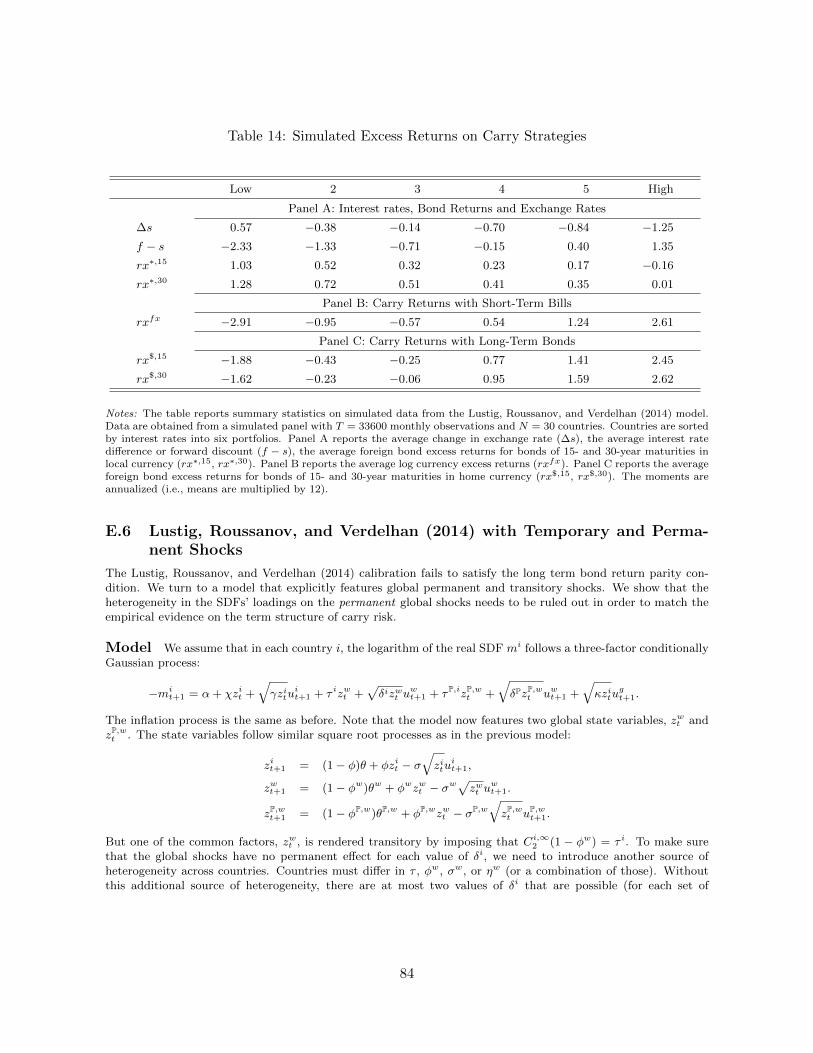
Table 14: Simulated Excess Returns on Carry Strategies

Low 2 3 4 5 High

Panel A: Interest rates, Bond Returns and Exchange Rates

∆s 0.57 −0.38 −0.14 −0.70 −0.84 −1.25

f − s −2.33 −1.33 −0.71 −0.15 0.40 1.35

rx∗,15 1.03 0.52 0.32 0.23 0.17 −0.16

rx∗,30 1.28 0.72 0.51 0.41 0.35 0.01

Panel B: Carry Returns with Short-Term Bills

rxfx −2.91 −0.95 −0.57 0.54 1.24 2.61

Panel C: Carry Returns with Long-Term Bonds

rx$,15 −1.88 −0.43 −0.25 0.77 1.41 2.45

rx$,30 −1.62 −0.23 −0.06 0.95 1.59 2.62

Notes: The table reports summary statistics on simulated data from the Lustig, Roussanov, and Verdelhan (2014) model.Data are obtained from a simulated panel with T = 33600 monthly observations and N = 30 countries. Countries are sortedby interest rates into six portfolios. Panel A reports the average change in exchange rate (∆s), the average interest ratedifference or forward discount (f − s), the average foreign bond excess returns for bonds of 15- and 30-year maturities inlocal currency (rx∗,15, rx∗,30). Panel B reports the average log currency excess returns (rxfx). Panel C reports the averageforeign bond excess returns for bonds of 15- and 30-year maturities in home currency (rx$,15, rx$,30). The moments areannualized (i.e., means are multiplied by 12).

E.6 Lustig, Roussanov, and Verdelhan (2014) with Temporary and Perma-nent Shocks

The Lustig, Roussanov, and Verdelhan (2014) calibration fails to satisfy the long term bond return parity con-dition. We turn to a model that explicitly features global permanent and transitory shocks. We show that theheterogeneity in the SDFs’ loadings on the permanent global shocks needs to be ruled out in order to match theempirical evidence on the term structure of carry risk.

Model We assume that in each country i, the logarithm of the real SDF mi follows a three-factor conditionallyGaussian process:

−mit+1 = α+ χzit +

√γzitu

it+1 + τ izwt +

√δizwt u

wt+1 + τP,izP,wt +

√δPzP,wt uwt+1 +

√κzitu

gt+1.

The inflation process is the same as before. Note that the model now features two global state variables, zwt andzP,wt . The state variables follow similar square root processes as in the previous model:

zit+1 = (1− φ)θ + φzit − σ√zitu

it+1,

zwt+1 = (1− φw)θw + φwzwt − σw√zwt u

wt+1.

zP,wt+1 = (1− φP,w)θP,w + φP,wzwt − σP,w√zP,wt uP,w

t+1.

But one of the common factors, zwt , is rendered transitory by imposing that Ci,∞2 (1 − φw) = τ i. To make surethat the global shocks have no permanent effect for each value of δi, we need to introduce another source ofheterogeneity across countries. Countries must differ in τ , φw, σw, or ηw (or a combination of those). Withoutthis additional source of heterogeneity, there are at most two values of δi that are possible (for each set of

84

parameters). 21 Here we simply choose to let the parameters τ differ across countries.

Bond Prices Our model only allows for heterogeneity in the exposure to the transitory common shocks (δi),but not in the exposure to the permanent common shock (δP). The nominal log zero-coupon n-month yield of

maturity in local currency is given by the standard affine expression y(n)t = 1

n

(Cn0 + Cn1 zt + Cn2 z

wt + Cn3 z

P,wt

),

where the coefficients satisfy second-order difference equations. Given this restriction, the bond risk premium isequal to:

Et[rx(i,∞)t+1 ] =

[C∞1 (1− φ)− χ+

1

2(γ + κ)

]zt +

1

2δizwt

+

[C∞3 (1− φP,w)− τP +

1

2δP − ηw

]zP,wt .

The log currency risk premium is equal to Et[rxFX,it+1 ] = (γ + κ)(zt − zit)/2 + (δ − δi)zwt /2. The permanent

factor zw,Pt drops out. This also implies that the expected foreign log holding period return on a foreign long bondconverted into U.S. dollars is equal to:

Et[rx(i,∞)t+1 ] + Et[rx

FX,it+1 ] =

[(C∞1 (1− φ)− χ)zit +

1

2(γ + κ)zt

]+

1

2δzwt

+

[C∞3 (1− φP,w)− τP +

1

2δP − ηw

]zP,wt .

Given the symmetry that we have imposed, the difference between the foreign term premium in dollars andthe domestic term premium is then given by: [C∞1 (1− φ)− χ] (zit−zt). There is no difference in long bond returnsthat can be traced back to the common factor; only the idiosyncratic factor. The spread due to the commonfactor is the only part that matters for the long-term carry trade, which approximately produces zero returnshere.

Foreign Bond Risk Premia Across Maturities To match short-term carry trade returns, we needasymmetric exposure to the transitory shocks, governed by (δ), but not to permanent shocks, governed by (δP).If the foreign kernel is less exposed to the transitory shocks than the domestic kernel (δ > δi), there is a largepositive foreign currency risk premium (equal here to (δ−δi)zwt /2), but that premium is exactly offset by a smallerforeign term premium and hence does not affect the foreign bond risk premium in dollars. The countries withhigher exposure will also tend to have lower interest rates when the transitory volatility zt increases, providedthat

(τ − 1

2δ)< 0. Hence, in this model, the high δi funding currencies in the lowest interest rate portfolios

will tend to earn negative currency risk premia, but positive term premia. The reverse would be true for thelow δi investment currencies in the high interest rate portfolios. This model thus illustrates our main theoreticalfindings: chasing high interest rates does not necessarily work at the long end of the maturity spectrum. If there isno heterogeneity in the loadings on the permanent global component of the SDF, then the foreign term premiumon the longest bonds, once converted to U.S. dollars is identical to the U.S. term premium.

Challenge The simulation of the LRV (2014) model highlights a key tension: without the heterogeneity inδs, the model cannot produce short-term carry trade risk premia; the heterogeneity in δs, however, leads tocounterfactual long-term carry risk premia. The decomposition of the pricing kernel suggests a potential route toaddress this tension: two global state variables, one describing transitory shocks and one describing permanentshocks. As noted in the study of the term structure models, the heterogeneity in the SDFs’ loadings on thepermanent global shocks needs to be ruled out in order to match the long term bond parity. The heterogeneity inthe SDFs’ loadings on the transitory global shocks accounts for the carry trade excess returns at the short end ofthe yield curve. We sketch such a model in the Online Appendix, and show that the heterogeneity in the SDFs’loadings on pure transitory global shocks can only be obtained if countries differ in more than one dimension (δ,but also τ , φw, σw, or ηw, or a combination of those parameters). A potential solution to the tension entails avery rich model that is beyond the scope of this paper. We leave the empirical estimation of a N -country modelthat replicates the bond risk premia at different maturities as a challenge for the literature.

21This result appears when plugging the no-permanent-component condition in the differential equation thatgoverns the loading of the bond price on the global state variable.

85

F Market Incompleteness

We want to verify whether our results are robust to market incompleteness. We consider a world in which foreigninvestors can only take positions in forward markets, but they cannot trade other foreign assets directly. Thistype of incompleteness introduces a wedge ηt+1 between the spot exchange rates and the pricing kernels:

St+1

St=Mt+1

M∗t+1

e−ηt+1 (34)

Obviously, we need to make sure that the Euler equations for the domestic and the foreign risk-free are satisfied:

Et (M∗t+1) = Et

(Mt+1

StSt+1

)= Et (M∗t+1e

ηt+1) = 1/Rf,∗t .

Et (Mt+1) = Et

(M∗t+1

St+1

St

)= Et

(Mt+1e

−ηt+1)

= 1/Rft ,

where we have used the relation in Equation (34) in the last equality. We implement these restrictions in atwo-country CIR model defined by the law of motion of the home and foreign SDFs:

− logMt+1 = α+ χzt +√γztut+1,

zt+1 = (1− φ)θ + φzt − σ√ztut+1,

− logM∗t+1 = α+ χz∗t +√γ∗z∗t u

∗t+1,

z∗t+1 = (1− φ)θ + φz∗t − σ√ztu∗t+1,

In this CIR model, Lustig and Verdelhan (2015) derive restrictions on the wedges that need to be satisfied inorder to rule out arbitrage opportunities in forward markets.

Proposition. In the CIR model, the incomplete market wedge ηt+1 (such that ∆st+1 = mt+1 − m∗t+1 − ηt+1)follows:

ηt+1 = ψzt + ψ∗z∗t −√

(γ − λ)ztut+1 +√

(γ∗ − λ∗)z∗t u∗t+1 +

√(λ− κ)ztεt+1 +

√(λ∗ − κ∗)z∗t ε

∗t+1, (35)

where the shocks εt+1 and ε∗t+1 are normally distributed as N(0, 1) and orthogonal to the SDF shocks ut+1 andu∗t+1. The law of motion of the wedge is determined by two parameters λ and λ∗ that satisfy λ ≤ γ and λ∗ ≤ γ∗.Once these two parameters are fixed, they determine the values of the remaining parameters κ ≤ λ, κ∗ ≤ λ∗, ψ,and ψ∗:

κ∗ = γ∗ −√γ∗√γ∗ − λ∗, (36)

ψ∗ =1

2(γ∗ − κ∗), (37)

κ = γ −√γ√γ − λ, (38)

ψ = −1

2(γ − κ). (39)

As noted in Proposition 3, when markets are complete and the long-term bond returns, once converted inthe same currency, are the the same, then the permanent components of the home and foreign SDFs are thesame, thus implying that nominal exchange rates are stationary in levels. When markets are incomplete, however,long-term bond returns, expressed in the same currency, could be the same, without implying that the permanentcomponents of the home and foreign SDFs are identical. When markets are incomplete, the ratio of foreign todomestic bond returns, expressed in the same currency is equal to:

R(∞),∗t+1

StSt+1

/R(∞)t+1 = eηt+1MP∗

t+1/MPt+1. (40)

Let us assume that the long-term bond return parity condition holds at each date, but that the ratio of thepermanent components of the SDFs is equal to the incomplete market wedge:

MPt+1/M

P∗t+1 = eηt+1 . (41)

86

In this case, the long-term bond return parity condition holds but the nominal exchange rate is not necessarilystationary in level. This counterexample to our main result, however, holds only in a knife-edge case. Recall thatin the CIR model, the permanent components of the home and foreign SDFs are:

MPt+1 = δ−1e−α−χzt−

√γztut+1e−B

∞1 [(φ−1)(zt−θ)−σ

√ztut+1],

MP∗t+1 = δ−1e−α−χz

∗t−√γ∗z∗t u

∗t+1e−B

∞∗1 [(φ−1)(z∗t−θ)−σ

√z∗t u∗t+1].

The ratio of the home and foreign permanent components is thus:

MPt+1/M

P∗t+1 = e−χ(zt−z∗t )−√γztut+1+

√γ∗z∗t u

∗t+1e−B

∞1 [(φ−1)(zt−θ)−σ

√ztut+1]+B∞∗1 [(φ−1)(z∗t−θ)+σ

√z∗t u∗t+1]

As noted in the Proposition above in Equation (35), the law of motion of the incomplete market wedge is:

ηt+1 = ψzt + ψ∗z∗t −√

(γ − λ)ztut+1 +√

(γ∗ − λ∗)z∗t u∗t+1 +

√(λ− κ)ztεt+1 +

√(λ∗ − κ∗)z∗t ε

∗t+1,

The ratio of the home to foreign permanent components of the SDFs can be equal to the incomplete marketwedge under some specific conditions. It must be that the wedge does not load on the orthogonal shocks εt+1 andε∗t+1 because those shocks do not affect the permanent components of the SDFs. This implies that λ = κ andλ∗ = κ∗. In order to satisfy the conditions in Equations (36) and (38), such constraints on the coefficients implythat κ = κ∗ = 0.22 Gathering these different conditions, it must be that the law of motion of the incompletemarket wedge is simply:

ηt+1 = −1

2γzt +

1

2γz∗t −

√γztut+1 +

√γ∗z∗t u

∗t+1.

In the class of CIR models, this is the only incomplete market wedge that can potentially be a counterexampleto our main claim. In order for Equation (41) to hold (and thus exchange rates to be non stationary in levelseven when the long-term bond return parity condition holds), the wedge must take this precise form and someadditional restrictions on the parameters of the CIR model must hold. In the CIR example above, it must bethat γ/2 = χ and B∞1 = B∞∗1 = 0. In this case, the exchange rate, ∆st+1 = mt+1 −m∗t+1 − ηt+1, is actuallyconstant and the term premium is zero.23 To sum up, one can certainly write an incomplete market model whereexchange rates are non stationary in levels even if the long-term bond return parity condition holds, but this willbe a knife-edge case in a large class of models.

22Note that the other solutions to Equations (36) and (38) imply that γ = κ and γ∗ = κ∗, which would implythat ψ = 0 and ψ∗ = 0, thus violating Equation (41) because the ratio of permanent SDFs does load on the statevariables zt and z∗t , whereas the wedge would not in this case.

23Note that the same result occurs even when countries differ in their impatience parameter, δ 6= δ∗. In thatcase, the ratio of the home and foreign permanent components becomes:

MPt+1/M

P∗t+1 = δ∗δ−1e−χ(zt−z∗t )−√γztut+1+

√γ∗z∗t u

∗t+1e−B

∞1 [(φ−1)(zt−θ)−σ

√ztut+1]+B∞∗1 [(φ−1)(z∗t−θ)+σ

√z∗t u∗t+1]

In order for Equation (41) to hold, it then must be that δ∗ = 0, χ = γ/2, B∞1 = 0 and B∞∗1 = 0, which againimply that the exchange rate is constant and the term premium is zero.

87