non-convex costs and capital utilization: a study of

Journal of Monetary Economics 45 (2000) 681}716

Non-convex costs and capital utilization:A study of production scheduling at

automobile assembly plantsq

George J. Hall*

Department of Economics, Yale University, New Haven, CT 06520-8264, USA

Received 2 November 1998; received in revised form 10 June 1999; accepted 21 July 1999

Abstract

I study detailed data from eleven automobile assembly plants. These data displayconsiderable cross-plant heterogeneity in production scheduling. To explain the ob-served heterogeneity, I solve a dynamic programming model. When desired production isbelow the plant's minimum e$cient scale, non-convexities induce production bunching;the plant uses less than full capital utilization on average and production is more volatilethan sales. When desired production is above the plant's minimum e$cient scale, theplant operates in a convex region of the cost curve. In this case, it uses high levels ofcapital utilization and production is less volatile than sales. ( 2000 Elsevier ScienceB.V. All rights reserved.

JEL classixcation: E23; D21; L23

Keywords: Inventories; Automobiles; Dynamic programming

qI am grateful to the Chrysler Corporation for providing much of data used in this paper. I havebene"ted from discussions with participants at numerous seminars, from comments made by SergioRebelo and several anonymous referees, and from conversations with John Cochrane, Bill Dupor,Martin Eichenbaum, Lars Hansen, Anil Kashyap, John Rust, Tom Sargent, Bob Schnorbus, andLewis Segal. Pier Deganello provided able research assistance. All remaining errors are mine.

*Corresponding author. Tel.: 203-432-3566; fax: 203-432-6323.E-mail address: [email protected] (G.J. Hall)

0304-3932/00/$ - see front matter ( 2000 Elsevier Science B.V. All rights reserved.PII: S 0 3 0 4 - 3 9 3 2 ( 0 0 ) 0 0 0 0 9 - X

1The minimum e$cient scale is the level of output that minimizes average cost.

1. Introduction

This paper studies how managers at automobile assembly plants organizeproduction across time. I formulate and solve a dynamic programming modelthat explains the production behavior observed from a new plant-level dataset.The model incorporates two non-convex margins: the adding and dropping ofan additional shift and the shutting down of the plant for a week at a time. Thesenon-convex margins play a central role in explaining much of the heterogeneityin production scheduling observed in the data. Speci"cally the model predictsthat when sales are below the plant's minimum e$cient scale (MES) managerswill use primarily non-convex margins to adjust output.1 Thus production willbe more variable than sales, and the plant's capital will sit idle much of the time.In contrast, when sales are above the plant's MES, managers will use convexmargins to adjust output; this production behavior is consistent with produc-tion as variable as sales and high levels of capital utilization.

I study a new database of fourteen automobile assembly plants. Eleven ofthese plants are the sole producers of various vehicle lines. For these elevenplants, weekly capital utilization and production date can be accurately alignedwith monthly employment, inventory, and sales data. These data display threefacts that a successful model of automobile production should capture.

1. For the average plant the workweek of capital is just 66.8 h. More strikingthough are the di!erences in capital utilization across plants. While theaverage workweek of capital for some plants is close to 100 h, it is less than15 h at other plants. Yet at all the plants the nominal premium for night workis modest, and the costs of having idle workers on the payroll are large.Workers on the second shift receive only about 5% more than workers on the"rst shift. Laid-o! workers from these plants receive 95% of their straighttime wage plus bene"ts.

Puzzling low levels of capital utilization are not unique to the autoindustry. The capital stock in U.S. manufacturing industries is employed, onaverage, fewer than 60 h per week (Shapiro, 1995). Shapiro argues that thetrue marginal premium for second shift work is closer 25%. Although thishigher marginal shift premium partially resolves the puzzle, the question stillremains: Why does the capital stock at some of these plants sit idle so much ofthe time?

2. At the average plant, the standard deviation of monthly production 21%larger than the standard deviation of sales. However, this production patternis not uniform across all the plants. At some plants production is about asvolatile as sales, while at other plants production is much more volatile thansales.

682 G.J. Hall / Journal of Monetary Economics 45 (2000) 681}716

2See Blinder and Maccini (1991) and the citations therein.

For a wide variety of industries, production is more volatile than sales.This fact has generated considerable attention since classic models of inven-tories, which assume convex short-run increasing marginal costs, imply that"rms should manage inventories such that production is smoother thansales.2 Although many explanations have been o!ered, there is no proposedanswer to the question: Why is production more variable than sales at someplants but not at others?

3. Plant managers rarely change the number of shifts or the line speed. Man-agers at some plants most frequently vary hours worked by using overtime.Managers at other plants most frequently vary hours worked by shuttingdown the plant for a week at a time. This production behavior is puzzlingsince the cost of laying o! workers is high.

Previous studies, such as Bresnahan and Ramey (1994), and Mattey andStrongin (1995), have documented the frequent use of short-term layo!s andinfrequent use of shift-changes and line-speed changes to vary output atmanufacturing plants. But this paper attempts to explain the observedheterogeneity in production scheduling of nearly identical plants. That is,why do some automobile assembly plants, but not others, use weeklongshutdowns so frequently to vary output?

Building on the work of Hamermesh (1989), Ramey (1991), Aizcorbe (1992),Cooper and Haltiwanger (1993), and Bresnahan and Ramey (1994), this paperargues that non-convex margins of adjustment play a key role in understandingthese facts. These non-convexities arise from two sources. First, the plant facesan integer constraint on the number of shifts that can be run. Second, there are"xed costs to opening the plant each week and running a shift. Additionally,provisions in the union labor contract (i.e., the required premium for overtimeand a pay #oor for short-weeks) create kinks in the plant's cost function. Theselabor contract provisions and non-convex margins produce large discontinuousjumps in the plant's cost curve. When desired production is below the plant'sMES, the plant operates in a non-convex region of its cost curve. In this region itis optimal for the plant to oscillate between periods of not producing andperiods of producing at its MES. This production behavior is consistent witha low average workweek of capital, production more variable than sales, andfrequent plant shutdowns. However, when desired production is above theplant's MES, the plant operates in a convex region of its cost curve, so the "rmwishes to smooth production and use high levels of capital utilization.

I solve a dynamic cost minimization model of an assembly plant managerwho takes the sales process as given. Consequently, I do not need to make anyrestrictive assumptions about the market structure or the nature of demand in

G.J. Hall / Journal of Monetary Economics 45 (2000) 681}716 683

3See Bresnahan (1981), Blanchard and Melino (1986), and Berry et al. (1995) for models of theautomobile industry in which both prices and quantities are endogenous.

order to solve the model. But the large automakers do behave as if they facedownward sloping demand curves for their products.3 So, this model can beviewed as a sub-problem which a pro"t-maximizing automaker solves whenchoosing from a menu of prices and quantities.

The formal analysis involves solving the dynamic cost minimization model fornine of the plants. I use the dataset to both parameterize the model and evaluatethe performance of the model. One of the advantages of modeling production atthe plant level is that several of the parameters do not need to be estimated; theyare simply drawn from the labor contracts. Other parameters are estimated tomatch moments of the employment and sales data. The results of this dynamicmodel demonstrate that much of the variation across plants in capital utilizationand relative variability of production and sales can be attributed to the ratio ofdesired production to the plant's minimum e$cient scale.

The rest of the paper is organized as follows. The second section providessome background information on how automobile assembly plants are run. Thethird section presents the dataset. The fourth section develops the intuitionbehind the model. The "fth section presents the dynamic programming model.In the sixth section parameter values are selected, the model is solved, andmoments implied by the model are compared to moments in the data. In the"nal section some concluding comments are made.

2. Some auto industry details

Although there is some variation across plants and "rms, most productiondecisions for automobile assembly plants are made at the monthly frequency.Once a month, there is a capacity planning meeting in which productionschedules are set. At this meeting managers are presented with last month's salesand inventory numbers and a sales forecast. The managers must then set andrevise their production schedule. They have "ve margins at their disposal.

The "rst margin is how many weeks the plant is scheduled to be open. Thesecond margin is how many days per week the plant is scheduled to be open.The third margin is the scheduled number of shifts per day. The fourth is thescheduled length (in hours) of each shift. The "fth margin is the rate of output orline speed, in jobs (vehicles) per hour. Scheduled monthly production is theproduct of these "ve margins:

jobs

month"

weeks open

month]

days open

week]

shifts

day]

hours

shift]

jobs

hour. (1)


The costs associated with manipulating these "ve margins di!er. Many of thesedi!erences are due to the structure of the labor contracts these plants operateunder.

Although production schedules are usually set at a monthly frequency,standard labor contracts are written with a one-week time period in mind. Theaverage straight-time, day-shift wage at these plants about is $18 an hour plusbene"ts. Workers on the second (evening) shift receive a 5% premium. Workerson a third (night) shift receive a 10% premium. Any work in excess of eight hoursin a day and all Saturday work is paid at a rate of time and an half. Employeesworking fewer than 40 h per week must be paid 85% of their hourly wage timesthe di!erence between 40 and the number of hours worked. This &short-weekcompensation' is in addition to the wages the worker receives for the hours s/heactually worked.

If the "rm chooses to not operate a U.S. plant for a week, the workers are laido!. After a single waiting week each year, laid-o!workers receive 95 cents on thedollar of their 40 h pay in unemployment compensation. Of this 95 cents, stateunemployment insurance (UI) pays about 60 cents. The remaining 35 cents ispicked up by supplemental unemployment bene"ts (SUB). Firms do not paylaid-o! workers directly, but laying o! workers does increase the "rm's experi-ence rating and UI premiums in the future. Anderson and Meyer (1993) andAizcorbe (1990) report that due to the cross-industry subsidies inherent in theUI system, "rms end up paying about half of the 60 cents coming from UI. Sincethe SUB is a negotiated bene"t between the "rm and the union, the "rmultimately pays all 35 cents. So, after the initial waiting week, it costs the "rmabout 65% of the 40 h wage to lay a worker o! for one week.

Unemployment insurance in Canada is slightly di!erent. For laid-o! Cana-dian auto workers there is a two-week waiting period each year before bene"tsare paid. These workers then receive 95% of their 40 h wage in unemploymentcompensation. Government unemployment insurance pays 55% of a worker'sfull-time earnings. The remainder is picked up by SUB. Unlike the U.S.,Canadian UI is not experience rated, so the "rm only pays the SUB portion.

Since 1992, several North American assembly plants have started to run threeseven-hour shifts per day. This allows the plant to be run 21 h a day. Workers atthese plants are paid eight hours of wages per day, Monday through Friday, fortheir seven hours of work. Therefore with no overtime, workers are paid a 40 hwage for working 35 h.

3. The data

This section describes a dataset of fourteen automobile assembly plants in theUnited States and Canada run by the Chrysler Corporation. The datasetcontains weekly production data from the "rst week of 1990 to the last week of


4Since Ward's and the MVMA aggregate the sales of the regular wheelbase minivans (Caravanand Voyager assembled at the Windsor facility) with the extended wheelbase minivans (GrandCaravan and Grand Voyager assembled at the St. Louis II facility), I use U.S. registration dataprovided by The Polk Company to decompose the Caravan and Voyager sales numbers.

5Aizcorbe (1992), Cooper and Haltiwanger (1993), Kashyap and Wilcox (1993), and Aizcorbe andKozicki (1995) also study plant-level data for automobile assembly plants but at the monthlyfrequency.

1994 and monthly employment, sales, inventory, and production data fromJanuary 1990 through December 1994.

For each assembly plant the following weekly data were collected: (1) thenumber of days the plant operated; (2) the number of days the plant was downfor holidays, supply disruptions, model changeovers, or inventory adjustments;(3) the number of shifts run; (4) the hours per shift run; (5) the scheduled jobs perday (line speed); and (6) the actual production for each vehicle line produced atthe plant. The Chrysler Corporation supplied data on 1, 3, 4, and 5. Data on2 and 6 were taken from Ward's Automotive Reports, Ward's AutoInfoBank, andAutomotive News.

For each vehicle line produced at these plants, monthly sales data werecollected. Total sales by vehicle line are the sum of sales by U.S. dealers,Canadian retail sales, and exports to the rest of the world. Sales by U.S. dealersare from Ward's. Canadian retail sales are from the Motor Vehicle ManufacturesAssociation (MVMA).4 Exports are from the American Automobile Manufac-turers Association (AAMA). For eleven of the plants, Chrysler provided thenumber of paychecks written each month. At these plants a pay-period is oneweek. So using the weekly data described above, I was able to constructa measure of employment for each plant.

Of the fourteen plants in the sample, eleven are single-source plants for at leastpart of the time. A single-source plant is a facility that is the exclusive producerof a set of vehicle lines. By restricting myself to single-source plants, I am able toline up inventory and sales data by vehicle line to employment, production, andhours worked by plant. This database is similar to the weekly database con-structed by Bresnahan and Ramey (1994).5 In particular the `six matchedplantsa in their sample are single-source plants.

The plants in the sample are listed in Table 1. Table 1 also reports whethereach plant is a single-source plant or not and the vehicle lines produced at eachplant. Only six of the fourteen plants (Dodge City, Newark, Pillette Road, StLouis II, Toledo I, and Windsor) produced the same vehicle line for the entire"ve year period. At the remaining eight plants, Chrysler changed the vehicle lineproduced during the sample period. So Chrysler could and did reallocate vehiclelines across its portfolio of assembly plants. But when Chrysler changed thevehicle line at a plant, the plant was closed for several months. Sterling Heightswas closed for four months when it switched from making the Daytona to the


Table 1Assembly plants and their vehicle lines

Period U.S. or Single Vehicle linesPlant (YR:M) Canada source?

Belvidere 90:1}93:5 U.S. Yes New Yorker Salon, Dynasty, FifthAve., Imperial

93:11}94:12 No NeonBramalea 90:1}91:12 Canada Yes Monaco, Premier

92:6}94:12 No Concorde, LHS, Vision, IntrepidBrampton 90:1}92:4 Canada Yes WranglerDodge City 90:1}93:5 U.S. Yes Ram Pickup, Dakota

93:7}94:12 No Ram Pickup, DakotaJe!erson North 92:1}94:12 U.S. Yes Grand CherokeeNewark 90:1}94:12 U.S. No Acclaim, Spirit, Intrepid, LeBaron

SedanPillette Road 90:1}94:12 Canada Yes Ram Van, Ram WagonSt. Louis I 90:1}91:5 U.S. Yes Daytona, LeBaron CoupeSt. Louis II 90:1}94:12 U.S. Yes Grand Caravan, Grand Voyager,

Town & CountrySterling Heights 90:1}94:3 U.S. No Daytona, Shadow, Sundance

94:8}94:12 No CirrusToledo I 90:1}94:12 U.S. Yes Cherokee, Commanche, WagoneerToledo II 90:1}91:6 U.S. Yes Grand Wagoneer

92:7}94:12 Yes WranglerToledo III 93:9}94:12 U.S. No DakotaWindsor 90:1}94:12 Canada Yes! Caravan, Voyager

!The Eurostar plant in Austria produced a version of the Voyager beginning in the fourth quarterof 1991 solely for the European market.

Sirrus; Belvidere was closed for "ve months when it switched from makingthe New Yorker to the Neon. It took three months to move productionof the Wrangler from Brampton to Toledo II. The length of these closuressuggests the presence of large technological frictions when switching vehiclelines across plants. In this paper, I do not address the issue of how Chryslerallocates vehicle lines across plants. Instead I take this allocation as "xed andfocus on explaining the three high-frequency features of the data listed in theintroduction.

Recall from Eq. (1) that scheduled output is the product of "ve margins.Table 2 reports by plant the percentage of weeks each of the "ve margins wereused. The plants are divided into four groups. The single-source plants are in the"rst three groups. The dual-source plants are in the fourth group. Since produc-tion of the Jeep Wrangler moved from Brampton to Toledo II in 1992, these twoplants are concatenated. A plant is counted as open for the week if it is up andrunning at least one day during the week. Otherwise it is counted as closed. If the


Tab

le2

Mar

gins

used

byea

chpla

nt!

Per

cent

age

ofw

eeks

inea

chst

ate

Wee

kscl

ose

dSh

ort

-wee

ksW

eeks

Wee

ks

Wee

ksSh

iftLin

esp

eed

Per

iod

inop

enH

OL

SUP

MC

IATO

TA

LH

OL

with

OT

chan

ges

chan

ges

Pla

nt(Y

R:M

)sa

mple

(1)

(2)

(3)

(4)

(5)

(6)

(7)

(8)

(9)

(10)

Je!er

son

Nor

th92

:1}94

:12

162

95.1

1.9

02.

50.

612

.312

.385

.81.

29.

3St

.Loui

sII

90:1}94

:12

261

95.0

1.9

03.

10

10.3

8.4

70.1

0.4

3.4

Win

dso

r90

:1}94

:12

261

93.1

1.9

04.

60.

49.

68.

462

.80.

43.

4

Bel

vide

re90

:1}93

:517

779

.72.

30

6.8

11.3

16.4

14.7

17.5

0.6

3.4

Bra

mpt

on/

Tol

edo

II90

:1}94

:12

249

88.0

2.0

03.

66.

414

.113

.339

.00

4.0

Dodg

eC

ity

90:1}93

:517

686

.92.

30

4.0

6.8

10.8

10.2

30.1

1.1

2.8

Pille

tte

Road

90:1}94

:12

261

77.4

1.5

0.4

9.2

11.5

16.5

14.9

13.8

06.

5Tole

doI

90:1}94

:12

261

83.1

2.3

0.8

5.7

8.0

13.0

11.9

22.2

06.

1

Bra

mal

ea90

:1}91

:12

101

38.6

1.0

05.

055

.411

.98.

90

01.

0St

.Loui

sI

90:1}91

:573

72.6

1.4

02.

723

.313

.712

.31.

40

2.7

Tole

doII

90:1}91

:677

35.1

1.3

1.3

5.2

57.1

10.4

6.5

2.6

00

Bel

vide

re93

:11}

94:1

260

93.3

3.3

1.7

1.7

016

.715

.033

.31.

75.

0Bra

mal

ea92

:6}94

:12

131

94.7

2.3

03.

10

13.0

10.7

64.9

03.

8D

odg

eC

ity

93:7}94

:12

7893

.65.

10

1.3

09.

07.

780

.82.

66.

4N

ewar

k90

:1}94

:12

261

84.3

1.5

05.

48.

814

.913

.034

.50

1.9

Ster

ling

Hei

ghts

90:1}94

:12

239

80.8

2.1

03.

313

.813

.412

.123

.40.

82.

5Tole

doII

I93

:9}94

:12

6794

.03.

00

3.0

011

.99.

055

.20

3.0

Ave

rage

plan

t83

.82.

00.

24.

69.

513

.011

.538

.50.

44.

0

!Note

:This

table

repor

tsth

eper

centa

geof

wee

ksea

chpla

ntis

ope

n,cl

ose

d,ru

nni

ng

ash

ort

-wee

kor

runnin

gove

rtim

e.The

pla

nt

closu

res

are

deco

mpo

sed

into

four

cate

gories

:H

OL"

holid

ay/v

acat

ion;

SUP"

supply

disru

ption;

MC"

mod

elch

ange

ove

r;IA

"in

vento

ryad

just

men

t.


plant is closed or open fewer than 5 d during the week, the primary reason forthe downtime is reported. Following Bresnahan and Ramey (1994), I usedinformation from Ward's Automotive Reports to classify each closure under one ofthe following categories: holiday or union dictated vacation (HOL), modelchangeover (MC), supply disruption (SUP), inventory adjustment (IA), or long-run closure (LRUN). Columns 2 through 5 in Table 2 report the number offull-week closures broken down by category. Long-run closures are not re-ported; a plant is classi"ed under a long-run closure if it is closed for more thanthree months in a row.

Weeklong shutdowns are frequent. Consider the bottom row of Table 2.The average plant was only open 83.4% of the available weeks. Thus theaverage plant was closed about 8 1/2 weeks each year. Weeklong shutdownsfor inventory adjustment account for most of this downtime. The averageshowever do not tell the whole story. Several of the plants, in particular Je!ersonNorth, St. Louis II, and Windsor, were rarely closed for inventory adjustment(or for any other reason). The vehicles made at these plants (sport utilityvehicles and minivans) have been among Chrysler's best sellers. In contrast, in1990 and 1991, Bramalea was closed more weeks for inventory adjustment thanit was open. During that time the slow-selling Premier and Monaco wereassembled there. This is also the case for Toledo II during 1990 and the "rsthalf of 1991 while the Grand Wagoneer (a slow seller) was assembled. Week-long shutdowns most frequently occurred at plants which made slow-sellingvehicles.

Table 2 also reports the percentage of weeks each plant was open for fewerthan "ve days. These are called &short-weeks'. In column 7, the percentage ofweeks each plant ran a short-weeks that was due to holidays is also reported.From these two columns, it is clear that almost all the short-weeks in the sampleare due to holidays. Many of the remaining non-holiday short-weeks areexplained by supply disruptions. Very few of these short-weeks are due toinventory adjustment. This is not surprising given the 85% short-week rule inthe union labor contract discussed above. This result supports similar "ndingsby Aizcorbe (1992) and Bresnahan and Ramey (1994).

Column 8 reports the percentage of weeks each plant used overtime. Theaverage plant used overtime during 38.5% of the weeks in the sample. Theplants which made the most extensive use of overtime (i.e., Je!erson North, St.Louis II, and Windsor) are the plants that rarely shut down for inventoryadjustment. In contrast several of the plants that rarely used overtime, such asBramalea (90:1}91:12), St. Louis I, and Toledo II (90:1}91:6), were frequentlyshut down for inventory adjustment. At plants such as Pillette Road and ToledoI both overtime and weeklong shutdowns is used to vary output. In general,overtime was used frequently, and the plants which made the Chrysler's mostpopular vehicle lines (minivans and sport utility vehicles) used overtime themost.


Table 3Average workweek of capital (in h/week)

Period d shifts Conditional ConditionalPlant (YR:M) run on open on not LRUN

Je!erson North 92:1}94:12 1, 2, 3 89.5 85.1St. Louis II 90:1}94:12 2, 3 104.4 99.2Windsor 90:1}94:12 2, 3 94.4 87.9

Belvidere 90:1}93:5 1, 2 73.7 58.7Brampton/Toledo II 90:1}94:12 1, 2 59.5 52.3Dodge City 90:1}93:5 2 81.6 71.0Pillette Road 90:1}94:12 2 78.0 60.4Toledo I 90:1}94:12 2 80.7 67.1Bramalea 90:1}91:12 1 36.3 14.0St. Louis I 90:1}91:5 1 38.2 27.7Toledo II 90:1}91:6 1 33.8 12.7

Belvidere 93:11}94:12 1, 2 80.4 75.0Bramalea 92:6}94:12 2 80.3 76.0Dodge City 93:7}94:12 1, 2 92.5 88.9Newark 90:1}94:12 2 83.2 70.2Sterling Heights 90:1}94:12 1, 2 80.4 64.9Toledo III 93:9}94:12 1 43.3 40.7

Average plant 74.5 63.1

Weighted average 80.0 66.8

Finally, columns 9 and 10 report the percentage of weeks a shift is added ordropped and the percentage of weeks a change in the line speed is made.Changes in the number of shifts were made rarely. Most of these change in thenumber of shifts and changes in line speed occur in the weeks immediatelyfollowing the introduction of new models and model changeovers.

Table 3 reports the number of shifts run and the average workweek of capitalfor each plant. The average workweek of capital conditioned on the plant notbeing under a long-run closure is presented in the far right column. Theaverage workweek of capital conditioned on the plant being open is presented incolumn 4. The three plants that were identi"ed as frequent users of overtime andinfrequent users of inventory adjustment (Je!erson North, St. Louis II, andWindsor) are plants which employed three shifts by the end of the sample. Notsurprisingly these three &3-shift plants' have the longest average workweeks ofcapital. The plants which rarely used overtime and were often closed forinventory adjustment, Bramalea (90:1}91:12), St. Louis I, and Toledo II(90:1}91:6), all ran 1 shift and have the shortest workweeks of capital.

Shapiro (1995) states that &the workweek of capital in U.S. manufacturingaverages less than 60 hours per week'. At the Chrysler plants, when the long-run


6 If long-run closures are not excluded, the average workweek of capital is 53.1 h. This is in linewith Shapiro's statement.

closures are excluded, the average workweek of capital is 66.8 h.6 This is in theballpark of Shapiro's statement. This "nding is also consistent with othermeasures of capital utilization reported by Shapiro. Shapiro (1993) reports thatfor manufacturing plants sampled by the Census' Survey of Plant Capacity from1977}1988 the average workweek of capital is 80.3 h/week. Using data from theBLS's Industry Wage Survey, Shapiro (1995) reports that the capital stock isutilized only 11.4 h per 24 h day for the industries he studies.

Shapiro (1995) "nds these low levels of capital utilization puzzling. So he asks,if second shift employees are paid only 5% more than their "rst-shift counter-parts, why do more "rms not employ second shifts? He partially answers thisquestion by providing evidence that the true marginal premium for night worksubstantially exceeds the nominal premium. Shapiro argues a better estimate ofthe shift premium is 25%. However the short average workweek of capitalreported here is not due to the plants' failure to run second shifts } all but threeplants ran more than a single shift. This short average workweek of capital islargely due to the plants being closed so much of the time. Conditional on theplants being open, the average workweek of capital is 80.0 h.

The di!erences in the average workweek of capital across the plants arestriking. At one extreme is Toledo II; while the Grand Wagoneer was beingassembled, the Toledo II facility averaged only 12.7 h of use per week. At theother extreme is St. Louis II; it ran, on average, almost 100 hours per week. Ifone thinks of 100 h per week as a lower bound on what is possible to utilizecapital, then the Toledo II facility utilized its capital only 12.7% of the timeavailable. The Pillette Road facility is perhaps more representative of thesample. Pillette Road was never down for a long-run closure during the sampleperiod but averaged only 60.4 h of use per week. So it utilized its capital less thantwo-thirds of the time available. The question still remains: Why is the level ofcapital utilization so low at so many of the plants?

Table 4 provides the means and standard deviations of the monthly produc-tion, sales and inventory data for the set of single-source plants. Total sales arethe sum of U.S. sales, Canadian sales, and exports to the rest of the world.Inventories are computed by a perpetual inventory method. Inventories arebenchmarked so that the inventories of discontinued vehicle lines are eventuallyzero. Inventories for all other vehicles lines are benchmarked using December1989 U.S. dealer inventory-to-sales ratios.

The three plants with the highest average levels of monthly production areWindsor, St. Louis II, and Je!erson North; these plants rarely closed andused overtime extensively. More interesting are the relative standard deviationsof production and sales. For all but four plants, the standard deviation of


Tab

le4

Mon

thly

stat

istics

:m

eans

and

stan

dard

devi

atio

ns

Pla

ntPer

iod

Pro

duct

ion

Tota

lsa

les

Inve

ntories

Inve

ntories

Tota

lsa

les

p 130$

6#5*0/

p 4!-%4

p 130$

6#5*0/

p 4!-%4

Je!er

son

Nor

th92

:1}94

:12

17,4

9016

,858

28,1

961.

7269

9277

290.

90St

.Loui

sII

90:1}94

:12

20,6

6920

,924

41,2

142.

1754

9952

081.

06W

indso

r90

:1}94

:12

24,1

9323

,230

65,4

062.

9567

7863

431.

07

Bel

vide

re90

:1}93

:514

,600

15,5

7532

,644

2.10

5479

3496

1.57

Bra

mpt

on/

Tol

edo

II90

:1}94

:12

5581

5790

11,2

812.

2319

6215

991.

23D

odg

eC

ity

90:1}93

:515

,851

17,2

4061

,707

3.69

4991

3502

1.43

Tole

doI

90:1}94

:12

12,6

4313

,464

29,4

252.

1339

4322

361.

76Pille

tte

Road

90:1}94

:12

6567

6603

18,8

503.

0527

0718

481.

47

Bra

mal

ea90

:1}91

:12

1783

2178

6781

3.96

1253

1172

1.07

St.Loui

sI

90:1}91

:564

1478

9827

,838

3.77

3208

2261

1.42

Tole

doII

90:1}91

:644

552

718

653.

9037

316

82.

22

Agg

rega

te90

:1}94

:12

103,

826

104,

420

266,

265

2.55

22,9

7017

,638

1.30


7The one exception is Bramalea. When Chrysler purchased American Motors from Renault,Chrysler agreed to build a minimum number of Premiers and Monacos (using Renault parts) atBramalea. Weak sales of these two vehicle lines forced Chrysler to o!er deep discounts eventually.Consequently the volatility of sales for these two vehicle lines is large.

8The production function in this model di!ers from the one studied by Lucas (1970), Mayshar andHalevi (1992) and Bils (1992) in two ways. In this model, the same number of employees work eachshift and the production function is generalized to allow for overhead labor. Allowing the number ofemployees to vary across shifts implies counter-factually that the line speed di!ers across shifts. Inmy dataset, I never observe a plant running di!erent line speeds on di!erent shifts.

9 I assume the wage schedule from the labor contract is allocative.

production is substantially greater than the standard deviation of sales. Notethree of the exceptions: Je!erson North, St. Louis II, and Windsor. For theplants that rarely shut down for a week at time but use overtime extensively,production is about as volatile as sales. For the plants which shut down forinventory adjustment more frequently, production is more volatile than sales.7The standard deviation of aggregate production over these eleven plants is 30%larger then the standard deviation of aggregate sales.

4. A static example

This section presents a simple one-period cost minimization problem ofa plant manager. Consider a plant in which the rate of production (the linespeed) is Cobb}Douglas in capital, k, and labor, n. The time period is one week.The plant must produce at least q goods. The plant can operate D days. It canrun one or two shifts, S, each day; both shifts are of length h. Let n employeeswork each shift. Workers on the "rst and second shifts are paid wage ratesw1

and w2, respectively. Assume there is a "xed cost to opening the plant and it

takes at least n62

employees per shift to produce any output.8The plant faces a standard labor contract.9 Given this contract, the plant

manager must choose how many days to operate the plant, how many shifts torun, how many hours to run each shift, and how many workers to employ oneach shift, to minimize the total cost of producing q. Formally, the managerwishes to:

minD,S,h,n

(w1#I(S"2)w

2)Dhn#max[0,0.85(w

1#I(S"2)w

2)(40!Dh)n]

#max[0,0.5(w1#I(S"2)w

2)D(h!8)n]

#max[0,0.5(w1#I(S"2)w

2)(D!5)(8)n]#d

subject to

q4DSh(k1~a(n!n62)a)


where I(S"2) is an indicator function. The parameter a is between 0 and 1. The"rst term in the objective function represents the straight-time wage paid toworkers on both shifts. The second term captures the 85% rule for short-weeks,and the third and fourth terms capture the overtime premium. The "fth term, d,is a "xed cost to opening the plant.

Production is linear in total hours worked but curved over employment.Without either the 85% rule for short-weeks or the requirement that at leastn62

employees work each shift, it would always be optimal to run both shifts sincethe marginal product of labor approaches in"nity as n!n6

2approaches zero.

However in the presence of these "xed costs, the plant can produce low levels ofoutput cheaper with a single shift than with two shifts.

Following the discussion in Section 2, I set w1"18.00 and w

2"18.90.

Since the time period is one week, I let D take on any integer between 0and 7 inclusive. Since most plants run either one or two shifts, I let S equal 1 or 2.I let hours per shift, h, vary between 7 and 10. I set k equal to 1, n6

2equal to

500, a equal to 0.56, and d equal to $250,000. The choice of d is discussed in moredetail below.

To illustrate the role non-convexities in the plant's cost function play in theallocation of labor, consider the following. Set D to 5 and h to 8. The managernow has two margins along which to vary output: the number of shifts and thenumber of employees (line speed). Conditional on the number of shifts chosen tobe run, the plant manager must set employment such that:

n(q,S)"Aq

DShk1~aB1@a

#n62

(2)

in order to produce q. The cost of producing q with S shifts is then

C(q,S)"(w1#I(S"2)w

2)Dhn(q,S)#d. (3)

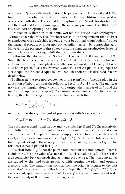
The cost curves conditional on one and two shifts, C(q,1) and C(q,2) respectively,are plotted in Fig. 1. Both cost curves are upward sloping, convex, and crosseach other once. The plant manager simply chooses to run a single shift ifC(q,1)(C(q,2) or to run two shifts if C(q,1)'C(q,2). Hence the total cost curvefor the plant, ¹C(q), is the envelop of the two cost curves graphed in Fig. 1. Thistotal cost curve is plotted in Fig. 2.

It is clear from Fig. 2 that the plant's total cost curve is non-convex. There isa kink in ¹C(q) at the value of q such that C(q,1) is equal to C(q,2). There is alsoa discontinuity between producing zero and producing e. The non-convexitiesare caused by the "xed costs associated with opening the plant and openinga second shift. The straight line coming from the origin is tangent to the costcurve at qH. Since the slope of this line is ¹C@(q*), then ¹C@(qH)qH"¹C(qH). Soaverage cost equals marginal cost at qH. Hence qH is the minimum e$cient scale,the level of output that minimizes average cost.


Fig. 1. Cost conditional on running one shift, C(q,1), and running two shifts, C(q, 2) holding hoursper shift "xed.

The hours-per-shift versus the shifts-per-day margin can be studied in a sim-ilar fashion. I set n to 1500 (so the line speed is set 48 vehicles per hours) and D to5. Hence the manager can now adjust the number of shifts, S, or the hours pershift, h. Conditional on the number of shifts run, the plant manager must set thehours per shift such that:

h(q,S)"q

DSk1~a(n!n62)a

(4)

in order to produce q. So the cost of producing q goods while operating a singleshift is

C(q,1)"w1Dh(q,S)n#max[0, 0.85w

1(40!Dh(q,S))n]

#max[0, 0.5w1D(h(q,S)!8)n]#d. (5)

And the cost of producing q goods while operating two shifts is

C(q,2)"(w1#w

2)Dh(q,S)n#max[0, 0.85(w

1#w

2)(40!Dh(q,S))n]

#max[0, 0.5(w1#w

2)D(h(q,S)!8)n]#d. (6)


Fig. 2. Total cost allowing either one or two shifts to run, ¹C(q), holding hours per shift "xed.qH denotes the minimum e$cient scale (MES).

The cost curves conditional on one and two shifts, C(q,1) and C(q,2) respectively,are plotted in Fig. 3. As in the previous exercise, both cost curves are upwardsloping and cross each other once. Each of these costs curves is not di!erentiableat two points. First, the 85% short-week rule and the "xed cost to opening theplant cause a discontinuity at zero. Second, the required overtime premiumcauses at kinks where hours per week equal 40. The total cost curve for theplant, ¹C(q), is the envelop of the two individual cost curves and is plotted inFig. 4. There is also a kink in ¹C(q) at the point where C(q,1)"C(q,2). Becauseof these non-di!erentiable points in the in ¹C(q), the MES is pinned down by"nding the unique line from the origin which intersects the cost curve only once.This line interests ¹C(q) at point A, the point associated with the plant runningtwo 40 h shifts.

In both of the above cases, a plant manager who must produce a level ofoutput q below the plant's MES (i.e. O(q(qH) would ideally like to takea linear combination of producing 0 and producing at the minimum e$cientscale, qH. Consider a plant which must produce a constant number x vehicleseach month. Assume there are four months in a week and x"3/4qH. The cost ofproducing x vehicles by evenly spacing production across the four weeks is4]¹C(3/4qH). However if the manager produces qH vehicles for three weeks andthus builds up an inventory level equal to x, the plant can then shut down duringthe fourth week and simply let inventories fall to zero. The cost of following this


Fig. 3. Cost conditional on running one shift, C(q,1), and running two shifts, C(q, 2), holdingemployment "xed.

second strategy is 3]¹C(qH). This is less than 4]¹C(3/4qH) since

¹C(3/4qH)3/4qH

'

¹C(qH)qH

,

which follows from the de"nition of minimum e$cient scale. When desiredproduction is less than the MES, the cost minimizing strategy involves produc-tion bunching and thus setting production would be more volatile than sales. Ifthe manager must consistently produce q above the plant's MES (i.e., q'qH)then the plant operates on a convex portion of the cost curve. In this regionthere is no incentive to bunch production and thus set production more volatilethan sales.

Because of the linearity and non-convexities of the total cost curve with"xed line speed plotted in Fig. 4, whether the MES occurs at point A (two40 h shifts) or point B (one 40 h shift) depends on the size of d. The straight line


Fig. 4. Total cost curve allowing either one or two shifts to run, ¹C(q), holding employment "xed.qH denotes the minimum e$cient scale (MES).

from the origin is tangent to ¹C(q) at point B rather than point A if(w

2!w

1)]D]h]n(d. Substituting in reasonable numbers yields:

($18.90!$18.00)]5]8]1500"$54,000(d. Suppose a plant must producefour shifts worth of output in three weeks. The manager will choose to operatetwo shifts for two weeks and close down for the third week if d'$54,000. Ifd($54,000, the plant will run two shifts one week and a single shift for twoweeks. One can see from Table 2 that shift changes rarely occur, but plants areoften completely shutdown for a week at a time. This suggests that the "xed costto opening the plant each week, d, is large.

5. The dynamic model

The above discussion appeals to the plant manager's ability to exploit bunchproduction without formally discussing a multi-period model. This sectionformulates a dynamic programming model of an automobile assembly plant. Asin the static example, the manager in the dynamic model controls the plant'slabor allocation (and thus production) to minimize the expected discounted costof production subject to technological constraints and the non-linear priceschedule for labor.


5.1. The dynamic program

As in the static model, the plant manager has access to a production techno-logy in which line speed is Cobb}Douglas:

qt"D

tStht[k1~a

t(n

t!n6

2)a] (7)

where 04a41. The variables qt, D

t, S

t, h

t, k

t, and n

tdenote the period t value

of the terms de"ne in the static example.The total number of workers the plant has on its payroll at time t is X

tnt#n6

1.

Let n61

denote the number of non-production workers (e.g. engineers, adminis-trative personnel) at the plant. Non-production workers are paid a "xed wageeach period and are never laid o!. Let X

tdenote the number of shifts of

production workers the plant has hired. So Xtnt

are the total number ofproduction workers hired. Individual production workers can only work oneshift. Production workers on the payroll who do not work either shift receiveunemployment compensation. This unemployment compensation is chargeddirectly and immediately to the "rm.

I impose the following restriction:

Stnt#n6

14X

tnt#n6

1. (8)

In words, the total number of employees working must be less than or equal tothe number of employees on the payroll. Each period the manager chooses thenumber of workers to have on the payroll next period.

The plant faces sales each period of st. Assume s

ttakes on one of three discrete

values and evolves according to a "rst-order Markov chain,

s(s, s@)"ProbMst`1

"s@, st"sN for s, s@3S"Ms

)*'), s

.%$*6., s

-08N.

Unsold output can be inventoried without depreciation. Let it`1

be the stock of"nished goods inventoried at the end of period t carried over into period t#1.Feasibility then requires that

qt#i

t5s

t#i

t`1. (9)

Inventories cannot be negative

it`1

50. (10)

Assuming the plant's labor contract is of the form described in Section 2, theplant's time t cost function is

C(t)"(I(St51)w

1#I(S

t52)w

2#I(S

t"3)w

3)D

thtnt

#max[0.0.85(I(St51)w

1#I(S

t52)w

2#I(S

t"3))(40!D

tht)n

t]

#max[0.0.5(I(St51)w

1#I(S

t52)w

2#I(S

t"3))D

t(h

t!8)n

t]

#max[0.0.5(I(St51)w

1#I(S

t52)w

2#I(S

t"3))(D

t!5)8n

t]

#uw140(X

t!S

t)n

t#dI(D

t'0)#40w

1n61, (11)


where w1, w

2, and w

3are the hourly wage rates paid to the "rst-shift, second-

shift and third-shift workers, respectively. I let u denote the fraction of the 40h day-shift wage charged to the "rm per idle employee. So the "rst termrepresents the straight time wages paid to the production workers. The second,third, and fourth terms capture the 85% rule for short-weeks and the requiredovertime premium. The "fth term is the unemployment compensation billcharged to the "rm. The sixth term denotes the "xed cost to opening the plant.The last term (seventh) are the wages paid to the plant's non-productiveworkers. This last term is a constant and has no e!ect on the manager'sallocation of labor. Let D

t"0 if and only if S

t"0.

The plant manager's problem is to minimize the present value of the dis-counted stream of costs given a constant real risk free interest rate, r. Assume thestock of capital, k

t, is "xed at kM for all t. The manager's problem is then to choose

a set of stochastic processes MXt`1

, it`1

, nt`1

,Dt,S

t, h

tN=t/0

to minimize:

E=+t/0A

1

1#rBtC(t) (12)

subject to (7)}(10) and given MX0, i0, n

0N. This minimization problem is split into

an intra-period problem and an inter-period problem. The intra-period problemis as follows. For each realization of MX

t, it, n

t, s

t, X

t`1, it`1

, nt`1

N the "rmchooses the feasible set, MD

t, S

t, h

tN, that minimizes (11). Let

C(Xt, it, n

t, s

t,X

t`1, it`1

, nt`1

)" minDt ,St ,ht

C(t) subject to (7), (8) and (9).

The inter-period problem is then solved by dynamic programming. Let<(X, i, n, s) be the optimal value function for the plant that has X shifts ofn employees on the payroll, carries inventories i into the period, and faces sales s.Thus, the plant's Bellman equation can be written

<(X, i, n, s)" minX{,i{,n{

GC(X, i, n, s,X@, i@, n@)#1

1#r+s{

s(s, s@)<(X@, i@, n@, s@)H(13)

subject to (10). The solution to this Bellman equation yields time invariantdecision rules.

5.2. Parameter values

The time period in the dynamic model is one week. The interest rate r is setsuch that (1#r)~1 equals 0.999; this corresponds to a 5% annual rate. I set thecapital stock, kM , to 1.0.

I estimated the parameters, a, n61, and n6

2with non-linear least squares using

the data on line speed and employment for each plant. The line speed data are


weekly and the employment data are the average number of paychecks writteneach month. After talking with Chrysler, I made the following assumptions:during weeks when plant i is open and during holiday weeks, S

itnit#n6

1iworkers are paid at plant i; during inventory adjustment weeks, supply disrup-tion weeks and long term closure weeks, n6

1iemployees are paid; during model

changeover weeks, n61i#n6

3iemployees are paid. So n6

3irepresents the number of

employees, above and beyond n61i

it takes to perform a model changeover atplant i. These assumption imply

Eit"

1

=Kt

[(OPit#H¸

it)(S

itnit#n6

1i)#(IA

it#SD

it#¸¹

it)n6

1i

# (MCit)(n6

1i#n6

3i)] (14)

where Eit

is the average number of paychecks written during month t at planti, S

it, the number of shifts plant i ran during month t, =K

t, the number of weeks

(pay-periods) during month t, OPit, the number of open weeks during month t at

plant i, H¸it, the number of holiday weeks during month t at plant i, IA

it, the

number of inventory adjustment weeks during month t at plant i, SDit,

the number of supply disruption weeks during month t at plant i, and ¸¹it, the

number of long-term closure weeks during month t at plant i.Eq. (14) states the average number of paychecks written each month equals

the total number of paychecks written divided by the number of pay-periods.Using the production function, Eq. (7) to eliminate n

it, I rewrite Eq. (14) as

Eit"n6

1i#

OPit#H¸

it=K

t

n62i#

MCit

=Kt

n63i#

(OPit#H¸

it)S

it=K

tA¸S

itkM 1~aiB

1@ai

(15)

where ¸Sit

is the average line-speed for the month at plant i. I estimatedn61i

, n62i

, n63i

, and ai, using Eq. (15) for all but four of the plants. The point

estimates are presented in Table 5; standard errors are reported in parentheses.Four of the plants in the sample underwent some form of major investment

during the time period I studied: Belvidere, Bramalea, and Sterling Heightsswitched vehicle lines; and Dodge City was down for nine weeks in 1993 fora major re-tooling. See Table 1. For these four plants, I allowed n6

1ito vary

across the two sub-periods. Speci"cally, I estimated

Eit"n6

1i#n6

4iD;M

it#

OPit#H¸

it=K

t

n62i#

MCit

=Kt

n63i

#

(OPit#H¸

it)S

it=K

tA¸S

itkM 1~aiB

1@ai


Table 5Parameter values for the production function

No. ofTime usable

Plant period obs. a n61

n62

n63

n64

R2

Belvidere 90:1}94:12 53 0.628 567 532 268 316 0.76(0.020) (159) (154) (369) (123)

Bramalea 90:1}94:12 60 0.707 196 670 20 599 0.93(0.039) (51) (113) (199) (71)

Brampton 90:1}92:4 27 1.0! 563 201 184 0.48(79) (44) (203)

Dodge City 90:1}94:12 53 0.616 1123 158 0" 1096 0.41(0.029) (228) (247) (191)

Je!erson North 92:1}93:5 49 0.620 364 658 1588 0.97(0.017) (54) (98) (348)

Newark 90:1}94:12 53 0.702 1405 596 268 0.47(0.062) (309) (191) (420)

Pillette Road 90:1}94:12 60 0.522 703 80 254 0.67(0.018) (140) (137) (170)

St. Louis I 90:1}91:5 10 0.767 894 409 0" 0.33(0.590) (301) (781)

St. Louis II 90:1}94:12 53 0.915 970 1005 2067 0.76(0.358) (231) (145) (624)

Sterling Heights 90:1}94:12 53 1.0! 708 772 253 283 0.53(195) (113) (563) (195)

Windsor 90:1}94:12 60 0.663 465 1121 1664 0.90(0.020) (187) (96) (288)

!To avoid estimates of aigreater than 1.0 for Brampton and Sterling Heights, I "xed a

ito be 1.0

prior to estimation."To avoid negative estimates of n6

2ifor Dodge City and St Louis I, I "xed n6

3ito be zero prior to

estimation.

where D;Mit

is equal to zero during the "rst sub-period, and is equal to oneduring the "rst sub-period. The results are also presented in Table 5.

The employment data were incomplete. I did not have employment data forthe Toledo plants. For six of the plants, seven months of employment dataduring 1990 are missing. Furthermore the sample period is short. So eventhough most of the point estimates are reasonable, caution is in order wheninterpreting any single point estimate.


10An estimate of a(1 is not inconsistent with Aizcorbe's (1992) "nding of increasing returns toscale at automobile assembly plants. Given my assumptions of of overhead labor and "xed costs,I am estimating a production with increasing returns to scale.

For all but two of the plants, the point estimates of the curvature parameter, a,are between 0.5 and 1.0. And most of the point estimates of a are within twostandard errors of 0.64, the usual estimate of labor's share.10 On average, thepoint estimates of n6

1and n6

4imply that about one-third of the workers at these

plants are non-production workers. The point estimates of n62

imply that at theaverage plant about one-half of the production workers on a shift are overheadworkers. Of course there is considerable variation in the parameter estimatesacross the plants.

I estimated the sales processes for each of the single-source plants by assum-ing that weekly sales follow an AR(1). I estimated the AR(1) parameters bymaximum likelihood. Since the sales data are monthly, I assumed weekly saleswere a latent variable and used the Kalman "lter to construct the likelihoodfunction. For each plant, I used Tauchen's (1986) method to compute weeklythree-state Markov chains whose sample paths approximate those of the esti-mated AR(1) processes. For each Markov chain, the grid width was chosen tomatch the standard deviation of actual sales process. The grid points were thenrounded to make them compatible with the inventory grid. To conserve onspace, the estimated Markov chains are not reported.

Following the discussion in the second section, wage rates are set as:w1"$18.00 per hour, w

2"$18.90 per hour, and w

3"$19.80 per hour. The per

idle employee fee for unemployment compensation, u, is set to 0.65 for the U.S.plants. For the Canadian plants, I set u"0.40. There is one remaining freeparameter, d, the "xed cost of opening the plant for the week. As discussed inSection 4, the "xed cost to opening a two-shift plant each week must be large. Ifthe "rm is operating in the non-convex region of its cost curve and the "xed costis small, then the model will predict that the manager will open and close thesecond shift rather than open and close the entire plant. So I set d to $1.0 million.

But what is this "xed cost, d? There are some "xed costs to opening the plant:warming up the equipment, and heating the shop #oor. Discussions fromindustry sources indicate that it is considerably easier to control many of thesecosts, particularly energy costs, by shutting down for a week at a time ratherthan sending a single shift home. Additionally, managers usually encouragesalaried workers to take vacation when the plant is shutdown. Thus the "rm canavoid having key workers on vacation when the plant is running.

But there may be other factors besides the "xed costs that in#uence themanager's decision whether to shut down the plant or just lay o! a single shift.The union contract dictates a strict hierarchy concerning who gets laid o! beforewhom. By laying the entire work force o!, the "rm treats all the workers equally


11See Aizcorbe's (1990) discussion of the UAW contract with Ford Motor Company.

12 In the model, a month is 13/3 weeks.

13When computing the MES for each plant I took into account the unemployment insurancepayment required if the plant shuts down for a week.

} thus saving the "rm the cost of "guring out who to lay o! and who to not.11More generally, if the workers face diminishing marginal utility in leisure, thenthe workers and the "rm may prefer a complete one-week shutdown over the"rm sending the second shift home for two weeks. While these other factors arecredible, the model assumes workers are homogeneous and is silent on workerpreferences.

Using the parameter values selected above, the intra-period problem is solvedvia grid search. The grids for D

tand S

tare set from 0 to 6 and from 0 to 3,

respectively, in increments of 1. The plant is closed for the week whenever St"0

or Dt"0. Recall, S

t"0 if and only if D

t"0. The shift length, h

t, can take on

values of 7, 8 or 9. So there are 84 grid points to evaluate for eachMX

t, it, n

t, s

t,X

t`1, it`1

, nt`1

N sept-tuple.To make the inter-period problem a "nite state, discounted dynamic pro-

gram, the state space is discretized. The number of shifts of workers on thepayroll, X

t, can take on values of 1, 2, or 3. For each plant, the level of

employment "xed to match the plant's observed average line speed. The in-ventory grid is allowed to vary across plants. For each plant, inventoriescan take on 501 points from 0 to 3]s

)*'). The inter-period problem is solved

by iterating on the Bellman equation, (13). Once the Bellman equation is solved,the transition matrix and the invariant probability distribution for thestate space are computed. The state space is checked to be ergodic. Popula-tion moments are computed using the invariant probability distribution and thedecision rules.

5.3. Results for nine plants

In this subsection, I use the production and sales parameters estimated aboveto solve the model plant-by-plant. A set of the model's predictions for each plantis reported in Table 6. The corresponding moments in the data are also reported.The "rst column of Table 6 reports the ratio of the monthly standard deviationof production to the monthly standard deviation of sales.12 The second columnreports the average weekly sales rate for the vehicles produced at each plant.This statistic is computed from the average monthly sales rate reported in Table4. The third column reports the minimum e$cient scale for the static model with"xed line speed parameterized for each plant.13 The fourth and "fth columnsreport the model's predictions for the average workweek of capital conditionalon the plant being open and unconditionally. Columns 6 and 7 report the


Tab

le6

Res

ults

for

the

nin

epla

nts

Ave

.w

orkw

eek

ofca

pita

l

Pla

nts

p .0/

.130$.

p .0/

.4!-%4

Ave

.w

eekl

ysa

les

MES

Con

d.

onop

enU

nco

nditio

nal

Unco

n.pr

ob

ofIA

wee

kU

nco

n.pr

ob

ofO

Tw

eek

Je!er

son

Nor

thM

odel

1.00

4296

89.3

89.3

0.0

54.7

Dat

a0.

9038

9389

.585

.11.

088

.1

St.Loui

sII

Mod

el0.

7343

0995

.295

.20.

081

.7D

ata

1.06

4832

104.

499

.20.

071

.5

Win

dso

rM

odel

0.83

5203

90.6

86.8

4.2

35.1

Dat

a1.

0753

6594

.487

.90.

463

.5

Bel

vide

reM

odel

1.09

4664

80.0

60.4

24.6

0.0

Dat

a1.

5735

9673

.758

.711

.917

.0

Bra

mpt

on

Mod

el1.

04R

82.2

65.9

19.9

6.9

Dat

a1.

2713

4678

.865

.112

.513

.3

Dodg

eC

ity

Mod

el0.

9644

1780

.169

.013

.90.

8D

ata

1.43

3982

81.6

71.0

7.4

21.1

Pille

tte

Road

Mod

el0.

9720

2380

.264

.819

.20.

7D

ata

1.47

1525

78.0

60.4

11.5

13.5

Bra

mal

eaM

odel

1.07

2566

40.0

15.7

60.7

0.0

Dat

a1.

0750

336

.314

.058

.03.

0

St.Loui

sI

Mod

el1.

0547

0940

.029

.825

.50.

3D

ata

1.42

1824

38.2

27.7

23.6

1.4


unconditional probabilities that the plant is closed for an inventory adjustmentor the plant is running overtime.

The model, with some exceptions, replicates the three facts described above.The model predicts that at the plants for which the average sales rates aregreater than the MES (i.e. Je!erson North, St. Louis II, and Windsor) produc-tion is less variable than sales, the average workweek of capital is over 85 h, andovertime is frequently employed. At the plants for which the average sales rateare less than MES, the model generally predicts that production is more variablethan sales, the plants use lower levels of capital utilization, and weeklongshutdown are frequent. The model also correctly predicts the number of shiftsused at each plant; the model predicts that Je!erson North, St. Louis II, andWindsor each run two or three shifts; Belvidere, Brampton, Dodge City, andPillette Road each run 2 shifts; and Bramalea and St. Louis I each run a singleshift.

Of course the dynamic model is too simple to match all the features of thedata. At all but two of the plants, the model under-predicts the standarddeviation of monthly production. In the data, weeklong shutdowns tend to bebunched together; the average duration of any type of weeklong closure (exceptsupply disruptions) is greater than one week. In the model, the duration ofa shutdown at most plants is one week. Since I aggregate each plant's output tothe monthly frequency, the e!ect of these single-week shutdowns tends to washout. The duration of the shutdowns is longer in the data, so their in#uence is notdampened as much by time aggregation.

Adding an accelerator term such as a desired inventory-to-sales ratio target tothe plant's cost function (Eq. (11)) can increase the implied duration of theweeklong shutdowns at these plants; this in turn implies an increase in thestandard deviation of monthly production. Furthermore adding an inventory-to-sales ratio target to the model can generate the inventory accumulationobserved in the data when sales increase. The work of Blanchard (1983) andKashyap and Wilcox (1993), as well as the auto industry's interest in days-supply statistics, suggest that automakers target such a ratio. Eq. (11) does notinclude such a target to isolate the e!ect the non-convex margins play inproduction scheduling.

These results are sensitive to relaxing the "xed line speed. If I let the plantmanager choose the line speed and shifts hired (n and X) once-and-for-all at time0, then at "ve of the plants (Je!erson North, St. Louis II, Windsor, Brampton,and Bramalea), the model dramatically over-predicts the line speed. This sug-gests that Eq. (7) may be a poor approximation to the true production techno-logy; given the estimated parameters there is too little curvature in employmentto rationalize the observed line speed at these "ve plants. An alternativeexplanation is that Eq. (11) is missing costs which increase with the line speed.For example, Ingrassia and White (1994) report that in 1972 GM set theline speed at the Lordstown assembly plant over 100 vehicles per hour. GM


14Once the manager chooses n and X, these variables are "xed for all t'0; but for each sales ratethe manager chooses new values of n and X.

eventually had to lower the line speed due increased worker discontent andincreased equipment breakdowns.

Finally in the model, the only reason the plant ever shortens the workweekis to reduce inventories. This assumption causes the model to ignore otherstates identi"ed in the data for which the plant might be shut down for all or partof the week. Thus the model is silent about holidays, model changeovers, andsupply disruptions. These limitations suggest some natural extensions to theanalysis.

Nevertheless the analysis illustrates that much of the heterogeneity in theproduction behavior across the nine plants can be explained by a simpledynamic programming model. Of course, since I allow some parameters to varyacross the plants, it is not clear how much of this cross-plant variation is due todi!erence in the parameter estimates and how much is due to the di!erences inthe mean of the sales process relative to the plant's MES. So in this followingsubsection, I resolve the model holding "xed all the parameters and varying justthe sales rate.

5.4. Results assuming a deterministic sales process

In this subsection, the sales process is deterministic; the transition matrix, s, isthe scalar 1. The remaining parameters are set at the values used for theBelvidere plant. The weekly sales rate varies from 200 to 7000 in increments of200. The employment and inventory grids are "xed throughout this exercise.

I solve the dynamic model at each sales rate. For each sales rate, I computethe average workweek of capital, the standard deviation of monthly production,and the total cost of production. The total cost for a given sales rate, ¹C(s), is thesum of the value function at each state, <(X, i, nDs), weighted by the uncondi-tional probability of each state, j(X, i, nDs). I multiply ¹C(s) by (1!b) to makethe units compatible with the static example. To compute a &long-run marginalcost' curve I allow the manager at each sales rate to choose n and X once-and-for-all at time 0.14 I trace out this long-run marginal cost curve for the plant bycomputing the one-sided derivative of the total cost curve. More precisely,

MC-3(s)"

(1!b)+X,i,n

j(X, i, nDs#200)<(X, i, nDs#200)!(1!b)+X,i,n

j(X, i, nDs)<(X, i, nDs)200

where MC-3(s) denotes the long-run marginal cost at sales rate, s.


Fig. 5. The long-run total cost curve.

15Even though the changes in the sales rate are permanent, I refer to the computed cost curves as&short-run' cost curves since I "x the &long-run' margins.

To compute a &short-run' cost curve, I "x the line speed, n, and number ofshifts hired, X, at their optimal levels for a sales rate of 3600 vehicles per week(the average rate at Belvidere). Thus the plant manager can only manipulate&short-run' margins: i

t, D

t, S

t, and h

t. Bresnahan and Ramey (1994) provide

evidence that line speed and shift changes are associated with permanentchanges in output while changes in the shift length and week-long shutdownsare associated with temporary changes in output.15 I then repeat the aboveexercise.

Consider the long-run analysis displayed in Figs. 5}8. Fig. 5 illustrates thatthe plant's cost total curve has both a concave and a convex region. Conse-quently the marginal cost curve, plotted in Fig. 6, is U-shaped: it is downwardsloping when sales are less than 3200 vehicles per week; it is essentially #at in theregion, 3200(sales rate(5000; and it becomes upward sloping when sales aregreater than 5000 vehicles per week. The minimum e$cient scale for the static


Fig. 6. The long-run marginal cost curve.

16 I take into account unemployment insurance when computing the MES.

model with "xed shift lengths (so the line speed is variable; see Fig. 2) andparameterized with the Belvidere parameter values is 4945 vehicles.16 Thus theBelvidere plant operates in a region of increasing long-run marginal costs onlywhen sales are greater than or equal to its static MES.

The concave region in the total cost curve occurs even though the managerhas the ability to manipulate inventories to exploit some of the non-convexitiesin the cost minimization problem. Two factors imply this concavity. First theproduction function, Eq. (7), does not exhibit constant returns-to-scale; it takesat least n6

2overhead workers to run a shift. Second the unemployment insurance

provision and the 85% short-week rule make it relatively expensive for the plantto operate at low levels. The marginal savings of laying o! a worker for oneweek is just 40(1!u)w

1; the marginal savings of reducing a worker's workweek

by one hour is just (1!0.85)w1. The combination of the minimum number of

workers needed to produce and the high costs associated with idling theseworkers imply a downward sloping marginal cost curve at low levels of output.


Fig. 7. Unconditional average work-week of capital (solid line) and the average workweek of capitalconditional on the plant being open (dotted line).

17Chrysler executives told me that when sales fall, they "rst adjust the price of vehicle (e.g. rebates,dealer-incentives) to try to increase sales; if demand is not su$ciently elastic, they then adjust output.Such a strategy is consistent with a U-shaped marginal cost curve.

18Although 5200 is greater than the plant's MES, the plant in this example continues to useweeklong shutdowns regularly at this sales rate because of the coarseness of the employment grid.

It is reassuring that the Belvidere plant sold on average about 3600 vehiclesa week, the nadir of the long-run marginal cost curve.17

The model predicts that when sales are 5200 vehicles per week or less, theplant manager primarily changes the frequency of weeklong shutdowns, a non-convex margin, to vary output.18 In this case, the optimal strategy is for theplant to produce for several weeks and build up an inventory stock equal to oneweek of sales; the plant then shuts down for a week and inventories fall to zero.Consequently, the plant manager chooses to make production volatile } despitethe fact that the sales rate is constant. See Fig. 8. Furthermore the optimalstrategy implies that capital often sits idle for a week at a time; note that inFig. 7 the di!erence between the unconditional average workweek on capitaland the workweek of capital conditional on the plant being open (the vertical


Fig. 8. Standard deviation of monthly output as a function of the weekly sales rate.

19Recall the production function, Eq. (7), is linear in hours worked.

20Given the "xed line speed, the plant can produce at most 6000 vehicles in one week.

di!erence between the dotted and solid lines) is quite large. The model alsocaptures the fact that when desired production is relatively high, the plantmanager primarily manipulates the shift length, a convex margin, to varyoutput. When sales are greater than 5200 vehicles per week, the plant is neverclosed for a week at a time. As Fig. 7 shows, the conditional and unconditionalaverage workweeks of capital are equal (and over 80 h) when sales are greaterthan 5200. Overtime is used extensively. Moreover the implied time series onproduction is relatively smooth; Fig. 8 illustrates that the standard deviation ofmonthly production falls when the sales rate rises above 5200.

When I "x the two long-run margins, the total cost curve becomes piece-wiselinear.19 See Fig. 9.20 When sales are below 4600, the plant manager changeshours worked (and thus output) by changing the number of weeks the plantoperates. When sales are above 4600 the plant manager changes hours workedby changing the shift length. Recall from Table 6 that the minimum e$cientscale for the static model with "xed line speed and Belvidere's parameter values


Fig. 9. The short-run marginal cost curve.

Fig. 10. The short-run marginal cost curve.


Fig. 11. Unconditional average workweek of capital (solid line) and the average workweek of capitalconditional on the plant open (dotted line).

is about 4600. Hence the marginal cost curve, plotted in Fig. 10, is not U-shaped;it is #at with one discontinuous jump at the plant's MES. The average workweekof capital becomes just a linear function of sales (Fig. 11). Fig. 12 illustrates thatthe standard deviation of monthly production falls when the plant varies outputusing overtime rather than weeklong shutdowns.

A simple dynamic programming model with credible non-convex margins ofadjustment can capture much of the heterogeneity in the production behaviorobserved across a set of automobile assembly plants. The model attributes thedi!erences across plants in capital utilization and relative volatility of produc-tion and sales to ratio of sales to the plant's minimum e$cient scale. A constantsales rate greater than the plant's MES implies that the plant is operating ina convex region of the cost curve, a sales rate below the plant's MES implies thatthe plant is operating in a non-convex region of the cost curve.

The model captures the fact that some plants, particularly those that maderelatively unpopular vehicles, often used weeklong shutdowns, a non-convexmargin, to vary output. Thus the model can explain why production at theseplants was more volatile than sales and why capital at these plants was oftenidle. At the same time, the model captures the fact that other plants, particularly


21However the work of Cecchetti et al. (1994) suggests that the transportation sector may not berepresentative of all manufacturing.

Fig. 12. Standard deviation of monthly output as a function of the weekly sales rate.

those that made relatively popular vehicles, primarily used convex margins ofadjustment such as overtime employment to vary output; therefore the modelcan explain why production at these plants varied by about as much as sales andwhy capital at these plants rarely sat idle. Thus, the model succeeds in reconcili-ng the three facts documented in the third section.

6. Concluding remarks

The paper focuses on understanding the high-frequency production behaviorof a small set of automobile assembly plants. Thus this paper trades generalityfor precise data. But the non-convexities identi"ed in this paper are not uniqueto automobile assembly plants. Managers at most manufacturing plants thatproduce-to-stock face these same non-convex margins: how many shifts to runand whether to open or close the plant each week. Thus the results of this papermay apply to other industries.21


It is unclear whether the important role non-convexities play at the plant leveldo not just wash out at the aggregate level. However, there is evidence thatproduction decisions are not independent across plants and "rms. Automobileassembly plants are just one component of a large network of suppliers anddealers. The work of Beaulieu and Miron (1991) and Cooper and Haltiwanger(1992) provide evidence that in the presence of strategic complementarities,multiple "rms synchronize output. These papers suggest that the dramatichigh-frequency variations in output observed at the plant level may not becompletely smoothed out by modest aggregation.

References

Aizcorbe, A., 1990. Experience rating, layo!s and unions: a look at U.S. auto assembly plant layo!s.Manuscript, Bureau of Labor Statistics.

Aizcorbe, A., 1992. Procyclical labour productivity, increasing returns to labour and labourhoarding in car assembly plant employment. Economic Journal 102, 860}873.

Aizcorbe, A., Kozicki, S., 1995. The comovement of output and labor productivity in aggregate datafor auto assembly plants. Working paper 95-33, Board of Governors of the Federal ReserveSystem.

Anderson, P., Meyer, B., 1993. Unemployment insurance in the United States: layo! incentives andcross-subsidies. Journal of Labor Economics 11, S70}S95.

Beaulieu, J.J., Miron, J., 1991. The seasonal cycle in U.S. manufacturing. Economic Letters 37,115}118.

Berry, S., Levinsohn, J., Pakes, A., 1995. Automobile prices in market equilibrium. Econometrica 63,841}890.

Bils, M., 1992. Measuring returns to scale from shift practices in manufacturing. Manuscript,University of Chicago.

Blanchard, O., 1983. The production and inventory behavior of the american automobile industry.Journal of Political Economy 91, 365}400.

Blanchard, O., Melino, A., 1986. The cyclical behavior of prices and quantities: the case of theautomobile market. Journal of Monetary Economics 17, 379}407.

Blinder, A., Maccini, L., 1991. Taking stock: a critical assessment of recent research on inventories.Journal of Economic Perspectives 5, 73}96.

Bresnahan, T., 1981. Departures from marginal-cost pricing in the american automobile industry:estimates for 1977}78. Journal of Econometrics 17, 201}227.

Bresnahan, T., Ramey, V., 1994. Output #uctuations at the plant level. Quarterly Journal ofEconomics 109, 593}624.

Cecchetti, S., Kashyap, A., Wilcox, D., 1994. Do "rms smooth the seasonal in production in a boom?theory and evidence. Manuscript, University of Chicago.

Cooper, R., Haltiwanger, J., 1992. Macroeconomic implications of production bunching: factordemand linkages. Journal of Monetary Economics 30, 107}127.

Cooper, R., Haltiwanger, J., 1993. The aggregate implications of machine replacement: theory andevidence. American Economic Review 83, 360}382.

Hamermesh, D., 1989. Labor demand and the structure of adjustment costs. American EconomicReview 79, 674}689.

Ingrassia, P., White, J., 1994. Comeback: The Fall and Rise of the American Automobile Industry..Simon and Schuster, New York.


Kashyap, A., Wilcox, D., 1993. Production and inventory control at the General Motors Corpora-tion during the 1920's and 1930's. American Economic Review 83, 383}401.

Lucas, R., 1970. Capacity, overtime, and empirical production functions. American EconomicReview Papers and Proceedings 60, 23}27.

Mattey, J., Strongin, S., 1995. Factor utilization and margins for adjusting output: evidence frommanufacturing plants. Working paper 95-12, Board of Governors of the Federal Reserve System.

Mayshar, J., Halevi, Y., 1992. On the time pattern of production: shiftwork, hours of work, andfactor employment. Manuscript, Hebrew University.

Ramey, V., 1991. Nonconvex costs and the behavior of inventories. Journal of Political Economy 99,306}334.

Shapiro, M., 1993. Cyclical productivity and the workweek of capital. American Economic ReviewPapers and Proceedings 83, 229}233.

Shapiro, M., 1995. Capital utilization and the marginal premium for work at night. Manuscript,University of Michigan.

Tauchen, G., 1986. Finite state markov-chain approximations to univariate and vector autoregres-sions. Economic Letters 20, 177}181.


non-convex costs and capital utilization: a study of

Documents