non-destructive resonance testing using … resonance testing using frequency and time domain...
TRANSCRIPT

Non-Destructive Resonance Testing
Using Frequency and Time Domain Techniques
by
Osama Jameel
A Thesis Presented in Partial Fulfillment of the Requirements for the Degree Master of Science in Technology
Approved October 2013 by the Graduate Supervisory Committee:
Sangram Redkar, Chair
Sharon Lewis Robert Meitz
ARIZONA STATE UNIVERSITY
December 2013
i
ABSTRACT
The objective of this thesis is to compare various approaches for classification of the
defective and non-defective parts via non-destructive resonance testing methods by
collecting and analyzing experimental data in the frequency and time domains. A Laser
Scanning Vibrometer was employed to measure vibrating samples in order to determine
the spectral characteristics such as natural frequencies and amplitudes. Statistical pattern
recognition tools such as Hilbert Huang, Fisher's Discriminant, and Neural Network were
used to identify and classify the unknown samples whether they are defective or not. In
this work, a Finite Element Analysis software packages (ANSYS 13.0 and NASTRAN
NX8.0) was used to obtain estimates of resonance frequencies in ‘good’ and ‘bad’
samples. Furthermore, a system identification approach was used to generate Auto-
Regressive-Moving Average with exogenous component, Box-Jenkins, and Output Error
models from experimental data that can be used for classification.

ii
DEDICATION
I dedicate this thesis to my committee chair, Dr. Sangram Redkar for his support and
encouragement, and my parents, Mr. Mahmood Jameel and Mrs. Naeemah Kadhim. For
their love and best wishes.

iii
ACKNOWLEDGMENTS
I would like to express my deepest gratitude and appreciations to my adviser and
committee chair, Dr. Sangram Redkar for his support, guidance during this journey, and
for teaching me the foundations of Non-Destructive testing and vibrations analysis. I
would like to acknowledge and thank Dr. Sharon Lewis for her help, support, and
motivation during my courses and thesis. I would also like to thank Dr. Robert Meitz for
providing me with great feedback and suggestions for my thesis.
Special appreciations and thanks to my great friends Alvaro Vargas-Clara, Pooja
Velaskar, and Dipika Subramanian for their unlimited support, encouragement, and
contribution in my thesis. Finally, I would like to thank my family for their love, support,
and caring throughout my life.

iv
TABLE OF CONTENTS
Page
LIST OF TABLES .............................................................................................................. …vi
LIST OF FIGURES ............................................................................................................... vii
CHAPTER
1 INTRODUCTION.............................................................................................. 1
Thesis Background .............................................................................. 1
Resonance Testing Using Laser Scanning Vibrometer ...................... 3
Problem Statement .............................................................................. 3
2 LITERATURE REVIEW .................................................................................. 5
3 LASER SCANNING VIBROMETER............................................................ 11
Resonance Testing ............................................................................. 11
Vibrometer Setup .............................................................................. 11
Experimental Samples ....................................................................... 19
4 ANALYSIS METHODS ................................................................................. 21
Modal Analysis Using Finite Element Analysis (FEA) ................... 21
Mathematical Model ......................................................................... 24
PSV Analysis ..................................................................................... 27
Discriminant Analysis ....................................................................... 28
Neural Network ................................................................................. 31
Hilbert Huang Transform .................................................................. 35
5 RESULTS ......................................................................................................... 39
v
System Model .................................................................................... 39
Fisher’s Discriminant Analysis ......................................................... 49
Neural Network Classification .......................................................... 50
PSV Frequency-Domian Comparison .............................................. 53
Hilbert Spectrum ............................................................................... 55
FEA Modal Response ....................................................................... 56
6 CONCLUSION ................................................................................................ 58
References ............................................................................................................................ 61

vi
LIST OF TABLES
Table Page
3.1 Aluminum Properties In SI Units ....................................................................... 19
4.1 Natural Frequencies For First Three Modes ...................................................... 24
5.1 Neural Network Results ..................................................................................... 52
5.2 NASTRAN Results ............................................................................................ 54
5.3 ANSYS Results .................................................................................................. 56

vii
LIST OF FIGURES
Figure Page
2.1 Digital Shearography System ............................................................................. 6
2.2 PSV Frequency Domain Data ............................................................................ 8
2.3 Micro-Scanning Vibrometer ............................................................................... 9
2.4 Good (Solid lines) and Defective (Dotted lines) parts ..................................... 10
3.1 Polytec Vibrometer System .............................................................................. 12
3.2 Laser Scanning Head ........................................................................................ 12
3.3 Optical Configration In Laser Scanner ............................................................ 14
3.4 Snapshot of Acquisition Interface .................................................................... 16
3.5 Time and Frequency Domian Response .......................................................... 17
3.6 PSV Display Mode ........................................................................................... 18
3.7 3D Mode Shape Display ................................................................................... 18
3.8 Defective Sample .............................................................................................. 19
4.1 Cantilever Beam ............................................................................................... 21
4.2 ANSYS Simulation of Defective and Non-Defective Samples ...................... 22
4.3 Neural Network Layers .................................................................................... 32
4.4 Feed-Forward Network with Two Layers ........................................................ 33
4.5 Neural Network Design in MATLAB ............................................................. 34
4.6 Confusion Matrix .............................................................................................. 34
4.7 Sifting Process .................................................................................................. 36
4.8 EMD Analysis for 9 IMFs ................................................................................ 36
4.9 Hilbert Spectrum ............................................................................................... 38

viii
Figure Page
5.1 ARMAX Block Diagram ................................................................................. 40
5.2 ARMAX Parameters Setting ............................................................................ 41
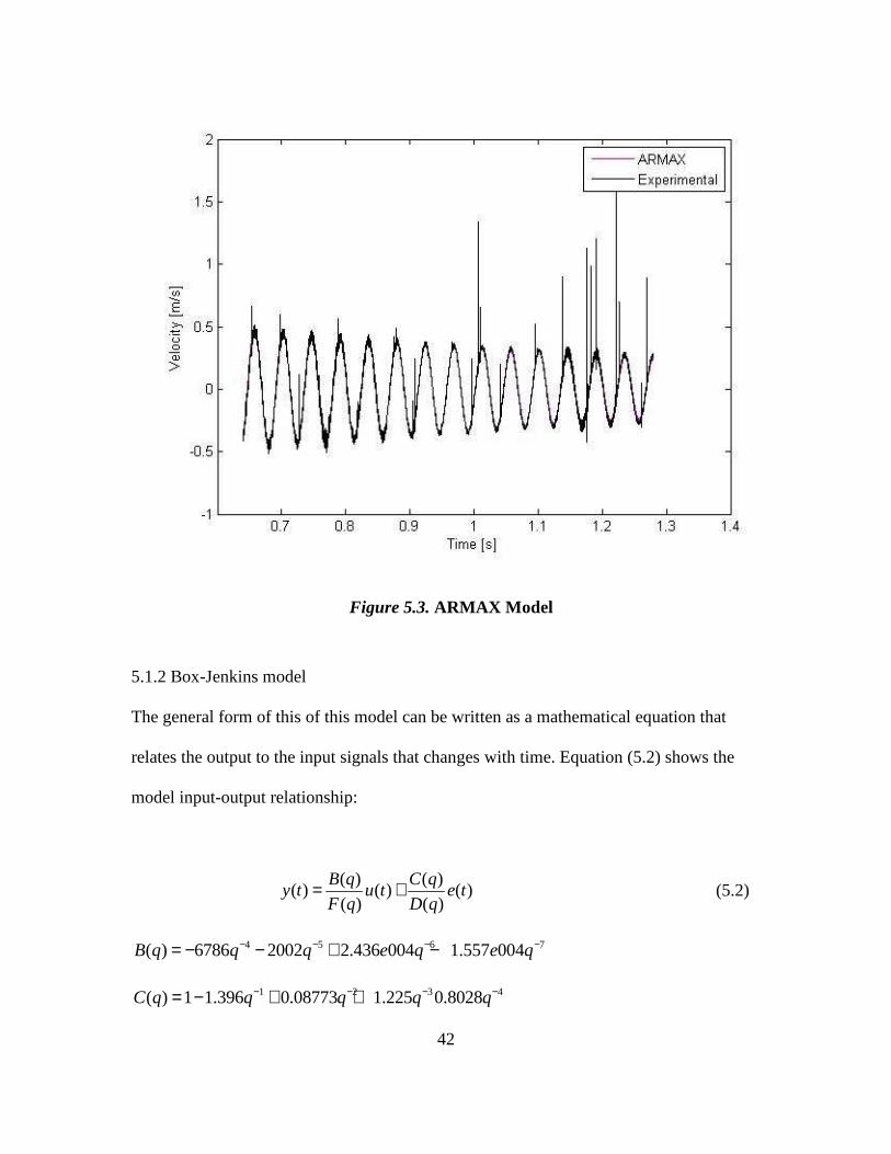
5.3 ARMAX Model ................................................................................................ 42
5.4 Box-Jenkins Block Diagram ............................................................................ 43
5.5 Box-Jenkins Parameters Setting ....................................................................... 44
5.6 Box-Jenkins Model ........................................................................................... 44
5.7 Outpu-Error Block Diagram ............................................................................. 45
5.8 Output-Error Parameters Setting ...................................................................... 46
5.9 Output-Error Model .......................................................................................... 47
5.10 Open-Loop Transfer Function ......................................................................... 48
5.11 Process Model .................................................................................................. 48
5.12 Fisher Non-Defective Sample .......................................................................... 49
5.13 Fisher Defective Sample ................................................................................... 50
5.14 Confusion Matrix of NN Classifier .................................................................. 51
5.15 NN Classification Accuracy ............................................................................. 53
5.16 PSV Non-Defective Sample ............................................................................. 54
5.17 PSV Defective Sample ..................................................................................... 54
5.18 Hilbert Spectrum Results .................................................................................. 55
5.19 IMF Results ....................................................................................................... 55

1
Chapter 1
INTRODUCTION
1.1 Thesis Background
Resonance testing is a method of Non-Destructive Testing (NDT). It can be used to
detect defects and flaws; such as cracks and voids in parts. Each product, with specific
dimensions and material properties, has its own resonant frequencies, but these
frequencies change in the presence of defects. These defects cause a difference in the
vibrational behavior (and the natural/resonant frequencies) due to the change in the
stiffness of the part. The change and variation in stiffness between the non-defective and
defective parts cause changes in the natural frequencies; under dynamical load, they
behave differently.
Traditional ‘destructive’ testing methods may include destroying some samples by
applying loads that are similar to the extreme working conditions in order to ensure the
safety and performance of the product while it is in service, these methods are called
destructive testing methods. Some of the disadvantages of destructive testing are high
cost due to the damaged parts, longer testing time, and the inability to test all the parts.
On the other hand, the testing method that do not require destroying any parts are called
NDT. The purpose of these methods is to identify and measure abnormal conditions,
especially microscopic defects and flaws, and to do so without deforming or destroying
the part (Price, Dalley, McCullough, & Choquette, 1997). These methods are quite
common in industry. Each NDT method has some advantages and disadvantages. The
simplest method is ‘visual inspection’. It is cheap and easy to perform, but it is incapable

2
of detecting internal defects. Some NDT methods require advanced technologies such as
X-rays, and laser which leads to expensive testing and requiring well-trained inspectors.
Testing is very important process in quality control; it is normally done at the final stages
of production to make sure that the products are qualified for performing the required
function before they get shipped to the costumer. Resonance testing provides important
information that can be used to identify good vs. bad parts.
In this work, an electro-dynamic shaker is used to excite the part and a Laser Scanning
Vibrometer is employed for gathering vibration data. This instrument uses holographic
interferometry which measures velocity and displacement of light wave; it has been used
in many applications such as automotive, aerospace, and biomedical (Santulli &
Jeronimidis, 2006). The advantages of using the Laser Vibrometer are the accuracy,
speed and no need for a physical contact with the part under test. The process consists of
a laser beam being directed at a product and by generating a mesh, the beam moves
through all the nodes of the mesh to complete the scan over all the points. Then the data
is collected at each point which can be in frequency or time domain. In the frequency
domain, the response is represented with respect to the frequency, while in the time
domain varies over time. The frequency and time domain are used in the system
identification tool box in MATLAB, which is a powerful tool that can be used to create a
model of a system by using the response data. The time domain data of good parts can
also be used to estimate the model.
In addition to system identification approach, pattern recognition methods can be
employed to recognize the good and bad parts. One of the methods is Hilber Huang
Transform (HHT). In this method, the non-linear non-stationary signal is decomposed

3
into nine harmonic signals then the frequency spectrum is evaluated from the extracted
time domain data. Another method used in this work is Fisher discriminant analysis, in
which good and bad frequency data are projected onto a line and then the difference
between the projected means shows the variations between the good and bad samples. In
addition, the neural network method is also employed for classification.
1.2 Resonance Testing Using Laser Scanning Vibrometer
Resonance testing has many advantages that make it efficient and beneficial to industry
more than other methods of testing; especially when the tests are performed by an accurate
powerful instrument such as the Laser Vibrometer. These advantages are:
1. The high accuracy of Laser Vibrometer allows for accurate testing results, and the
velocity and displacement data can be collected which makes it easy to analyze.
2. A mesh of small elements connected by nodes can be generated to ensure that the
‘automated multipoint’ test can be performed at each small segment of the part to be
tested.
3. This NDT method is fast and it can be used in a large product’s inspection line.
4. The high frequency range helps define small and large defects.
5. No contact is required with the part under investigation. This property helps performing
the test from distance or for complex geometry design products.
1.3 Problem Statement
This thesis concentrates on identifying the defects and flaws in the products and machine
parts using resonance NDT methods in both frequency and time domains by employing
laser vibrometry scanning technology. It also includes a comparison between defective
and non-defective test samples by analyzing the data from experiments. Furthermore, an

4
ideal theoretical analyses are used by employing numerical software packages ANSYS
and NASTRAN NX8.0.
The objectives of the thesis are accomplished by:
1. Describing the difference between frequency and time domains and explaining the
fundamental operating principles of the Vibrometer.
2. Performing the experiments using the laser scanning Vibrometer and electro-
dynamic shaker.
3. Applying different types of vibrational waves such as burst chirp, white noise, and
sinusoidal sweep waves, then comparing the results of their response.
4. Generating mathematical models using time domain data for the part under
investigation using MATLAB system identification tool box.
5. Identifying Defective and non-Defective parts, analyzing the experimental results,
using frequency domain data.
6. Generating a finite element simulation using ANSYS NASTRAN NX8.0 software
packages for both the defective and non-defective parts
7. Using pattern recognition tools such as neural network, Fisher’s discriminant
analysis, and Hilbert Huang Transform to classify the experimental data.

5
Chapter 2
LITERATURE REVIEW
The outcome of each NDT method depends on the technology and the testing method
type. Selecting the testing method is based on the cost and time required for the test.
Some methods are very cost effective but they are less accurate such as visual inspection
method. Historically, this method was used in a study conducted to identify the saw
marks in wood materials; the testing result was either a “Yes” for the good parts or a
“No” for the defective parts. The sliding scale was used to identify the level of defects by
choosing a range from 1 to 10, in which 1 represents the minimum, while 10 is the
maximum (Smith, Callahan, & Strong, 2005).
Newer testing technologies based on spectroscopy use ultrasonic NDT methods. The
fundamental principle of this method is based on the ultrasonic wave propagation through
the part; these waves are of such high frequency that they exceed the human hearing
ability. The wave penetrates the part at certain characteristics such as specific velocity
value; any reflection of this wave indicates a defect or flaw in the part’s material (IAEA,
2001). (Characteristics such as velocity and displacement can be measured to detect the
presence of flaws in the part)
Another method called Damage Locator Vector (DLV) has been used to detect the flaws
and damage in the part’s material. This method is based on vibrational testing by using
the frequency response function. The defective part is identified due to change in the
stiffness when compared to the good part (Huynh & Tran, 2004).
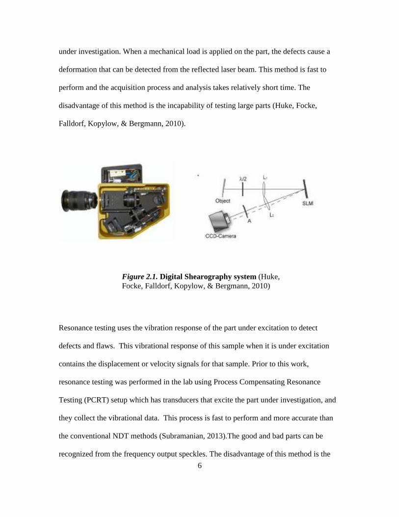
Another method of NDT is called the Shearography, which is used to define the invisible
defects. The principle of this technique is based on applying a laser beam on the part
6
under investigation. When a mechanical load is applied on the part, the defects cause a
deformation that can be detected from the reflected laser beam. This method is fast to
perform and the acquisition process and analysis takes relatively short time. The
disadvantage of this method is the incapability of testing large parts (Huke, Focke,
Falldorf, Kopylow, & Bergmann, 2010).
Resonance testing uses the vibration response of the part under excitation to detect
defects and flaws. This vibrational response of this sample when it is under excitation
contains the displacement or velocity signals for that sample. Prior to this work,
resonance testing was performed in the lab using Process Compensating Resonance
Testing (PCRT) setup which has transducers that excite the part under investigation, and
they collect the vibrational data. This process is fast to perform and more accurate than
the conventional NDT methods (Subramanian, 2013).The good and bad parts can be
recognized from the frequency output speckles. The disadvantage of this method is the
Figure 2.1. Digital Shearography system (Huke, Focke, Falldorf, Kopylow, & Bergmann, 2010)

7
contact between the part and the transducer which makes it difficult to test complex
geometry parts.
Recently, a continuous laser scanning via Laser Doppler Vibrometry (LDV) was
performed on a wind turbine to analyze the vibrational characteristics. The response was
measured to identify the mode shapes of the moving turbine (Yang & Allen, 2012). This
method used the Vibrometer on rotating parts.
LDV is a device used for measuring vibrational characteristics of a structure under
vibration loading. It has been used in recent years in aerospace (aircraft composite
structure defects analysis), automotive, and biological materials such as fruits (Santulli &
Jeronimidis, 2006). The results show the velocity amplitudes of fruits under excitation, if
these amplitudes are in the acceptable frequency range, the fruit could be considered as
good. An experiment was conducted by employing the LDV to analyze the linearity and
nonlinearity of vibration characteristics to detect the defects and flaws in the deformed
structures (Vanlanduit, Guillaume, Schoukens, & Parloo, 2006).
The dynamic vibrations and Echo tests are performed in many engineering fields such
as civil engineering to define the imperfection of the products and material. In these types
of tests, a pulse wave is used to excite the part or the structure by a hammer, the analysis
of this method is applied by observing and analyzing the reflected waves (Wong &
Toppings, 1988). Using the Vibration modal analysis started in the 1970’s when the FFT
analyzer was developed during that time (Schwarz & Richardson, 1999). It is very
important to understand and define the resonance frequencies of a part or structure
because at some of these frequencies the structure can have a high amplitude response
that can cause the structure damage. In a recent paper, a new testing approach using the

8
Laser Scanning Vibrometer was used to detect the flaws in the material (Breaban,
Carlescu, Olaro, & Gh. Prisacaru, 2011). In this experiment a PSV-300 laser Vibrometer
was used to measure the micro displacement in a velocity response form of the polymers
as illustrated in Figure 2.2. In this experiment, a white noise vibration signal was used to
identify the resonance frequencies of the part under investigation (Breaban, Carlescu,
Olaro, & Gh. Prisacaru, 2011).
Laser Vibrometer can be used for micro-scanning, by coupling the scanning head to a
microscope in order to get very small laser beam diameter (1 µm) for measuring non
periodic motions. This technology has been applied for testing gyroscopes, micro
switches, and micro motors (Traynor). The setup of this system is shown in Figure 2.3.
Figure 2.2. PSV Frequency Domain Response (Santulli & Jeronimidis, 2006)

9
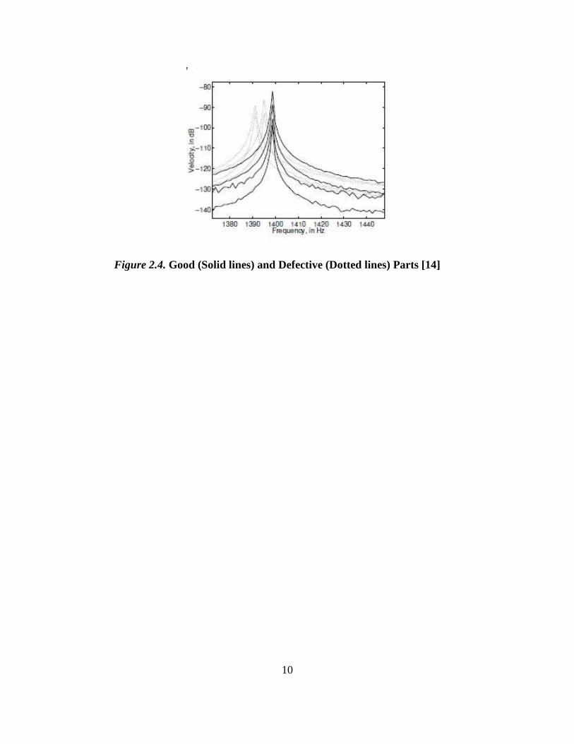
Many techniques have been used to analyze the vibration testing data. In the paper by
Vanlanduit et al Singular value decomposition (SVD) was proposed as a classification
method, the robust SVD employed for this purpose and applied on aluminum testing data
under different conditions such as fatigue, saw cut, covered with plastic, and covered
with acoustic material. Most of the work was focused on a good part and defective cases,
one with small fatigue crack and the other with large fatigue crack (Vanlanduit, Parloo, &
Guillaume, A Robust Singular Value Decomposition to Detect Damage Under Changing
Operating Conditions and Structural Uncertainties). Fig 2.3., illustrates the difference in
the peaks among the good and defective parts.
Figure 2.3. Micro-Scanning Vibrometry (Traynor)
10
Figure 2.4. Good (Solid lines) and Defective (Dotted lines) Parts [14]
11
Chapter 3
LASER SCANNING VIBROMETER
3.1 Resonance Testing
Resonance testing is a form of NDT testing in which the part under investigation is
subjected to vibrational excitation. Resonance frequencies represent a property of part or
structure, the value of these frequencies depends on the material type, stiffness and
boundary conditions of that structure (Schwarz & Richardson, 1999). The response of the
vibration can be obtained in two forms, the time domain and frequency domain.
3.2 Vibrometer Setup
Laser Scanning Vibrometer is an instrument that uses laser beam to measure velocity of
two dimensional surfaces. In this work, the main purpose of using this instrument is to
measure the velocity response of a part under excitation. The generated wave in the
controller can be selected in different forms such as Sinusoidal Sweep, Burst Chirp,
White Noise and Square waves. The instrument is equipped with a velocity decoder that
decodes the velocities in the controller unit. The range of the wave’s frequencies is from
0.01 Hz to 30 MHz (Polytec). This instrument is ideal for testing parts where it is
difficult to place an accelerometer like turbine blades and any other parts under vibration
or movement effects.
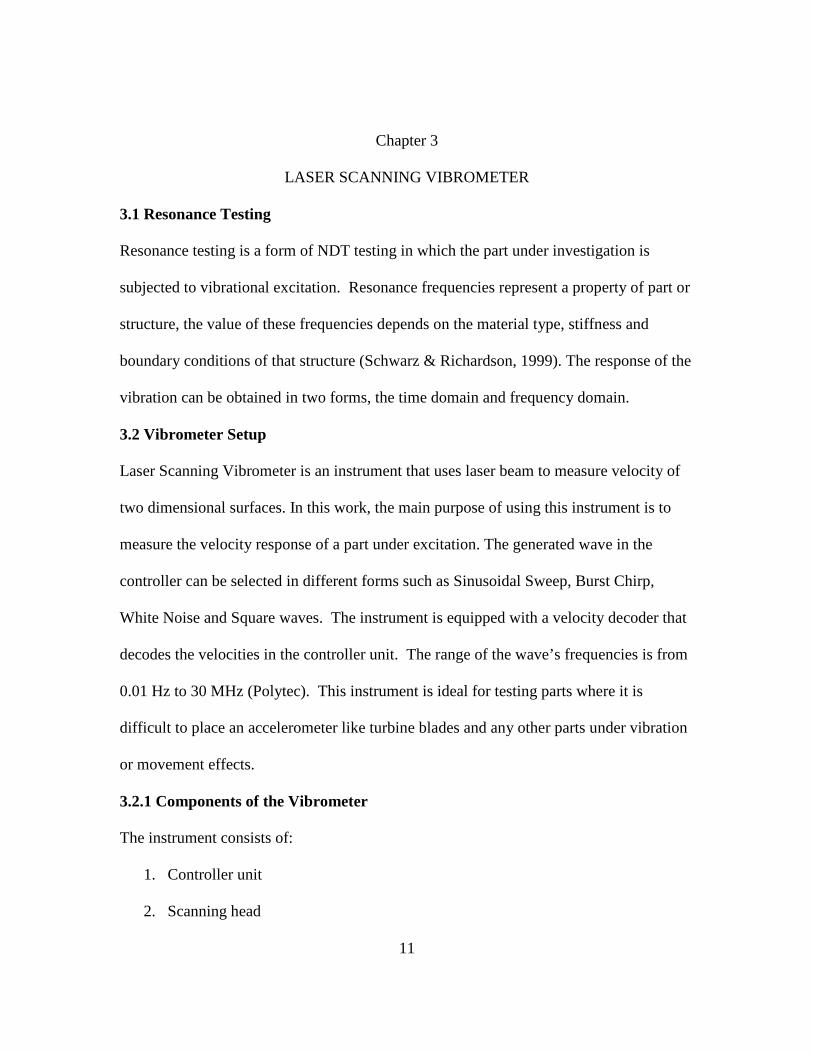
3.2.1 Components of the Vibrometer
The instrument consists of:
1. Controller unit
2. Scanning head
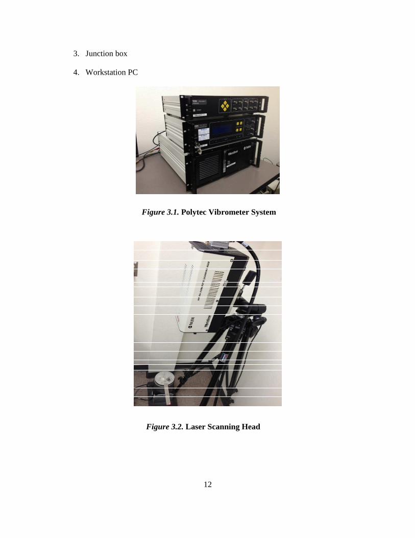
12
3. Junction box
4. Workstation PC
Figure 3.1. Polytec Vibrometer System
Figure 3.2. Laser Scanning Head
13
The controller unit generates the vibration signal and decodes the velocity output signal
of the part under investigation. The scanning head has interferometers to reflect the laser
beam. The connection interface between the units is provided by the junction box which
connects the controller to the workstation PC. The PC is provided with Polytec Scanning
Vibrometer (PSV) software, this software has the ability to generate a scanning mesh
points and has multiple scanning options such as continuous, single shot, and mesh
scanning.
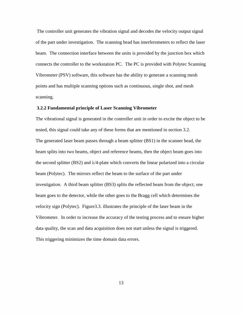
3.2.2 Fundamental principle of Laser Scanning Vibrometer
The vibrational signal is generated in the controller unit in order to excite the object to be
tested, this signal could take any of these forms that are mentioned in section 3.2.
The generated laser beam passes through a beam splitter (BS1) in the scanner head, the
beam splits into two beams, object and reference beams, then the object beam goes into
the second splitter (BS2) and λ/4-plate which converts the linear polarized into a circular
beam (Polytec). The mirrors reflect the beam to the surface of the part under
investigation. A third beam splitter (BS3) splits the reflected beam from the object; one
beam goes to the detector, while the other goes to the Bragg cell which determines the
velocity sign (Polytec). Figure3.3. illustrates the principle of the laser beam in the
Vibrometer. In order to increase the accuracy of the testing process and to ensure higher
data quality, the scan and data acquisition does not start unless the signal is triggered.
This triggering minimizes the time domain data errors.
14
3.2.3 Advantages of using Laser Scanning Vibrometer
Laser Vibrometer provides many advantages when compared to other vibrational signal
generators and acquisition systems.
1. No surface contact is required
2. A signal can be generated in the same system
3. The system uses safe helium laser
4. Can measure velocities at multiple ranges (µm/s to 30 m/s) and displacement (nm
to more than 41 mm)
5. Acquire data and triggers signal at the same time.
Figure 3.3. Optical Configurations in Laser Scanner (Polytec)

15
3.2.4 Polytec Scanning Vibrometer (PSV) software
The part under investigation has to be attached to the shaker, and then the laser beam has
to be pointing at the surface of the part. A mesh consists of many nodes is generated on
the surface, this allows the laser beam to move at each point while sweeping the part at
certain frequency range. In this project, the signal types are Burst Chirp, Sinusoidal, and
White Noise with frequency range of (0-5) KHz. While sweeping the part with each
signal separately, the laser beam starts the data acquisition at each point of the mesh until
all points are scanned. The data in the PVS software is in two forms, time domain data
(velocity vs. time) and frequency domain (velocity vs. frequency). Both data can be
analyzed in the PVS to determine the mode shapes and amplitudes for the good and
defective parts, the data can exported as a text file to be analyzed in MATLAB.
The PVS software has two modes, one is the acquisition, and the other is the presentation
mode. The acquisition mode has a live video image of the part on which the laser beam
can be moved to positions where the alignment of coordinates occur, then the mesh can
be defined on the part in squares or triangular shapes. The mesh divides the part into
many elements and each element has node at each corner that connects it to the neighbor
element.

16
In the acquisition mode, the setting has to be completed before running the test. Two
important settings have to be set, the first is to select the frequency range, and the second
is selecting the amplitude and wave type.
The output of the test is showing in small windows called analyzer. The output type can
be selected as velocity or displacement in frequency or time domain, the analyzer is on
X-Y coordinates. The scanning process starts with points alignment by selecting points
on the objective surface, then moving the laser beam to ensure high laser concentration
on the surface in case of surface flatness problems. Then, the next step before scanning
process is applying the mesh on any required area of the object. Once these settings are
completed, the acquisition process can start by sweeping all the nodes of the mesh.
Figure 3.4. Snapshot of Acquisition Interface

17
The second mode of the PVS software is the display mode in which the analysis on the
data can be performed such as selecting the highest amplitudes, define the mode shapes,
and calculating the magnitude and phase of the velocity and displacement signals. The
output can be displayed in 2D, 3D, animation, or single points. Any of these display
methods can be applied on the velocity or displacement output.
Figure 3.5. Time and Frequency Domain Response
a- Time Domain b- Frequency Domain

18
Figure 3.6. PSV Display Mode
Figure 3.7. 3D Mode Shape Display

19
3.3 Experimental Samples
The samples are made of aluminum-6061 T6 which has the properties listed in Table 3.1.
Property Value
Density 2700 Kg/m3
Modulus of Elasticity 68 Gpa
Poisson’s Ratio 0.33
The dimensions of the samples are 201.68 mm X29.337 mm X 1 mm. The defective
parts have a hole of 6.35 mm diameter, the center of the hole is located at distance 93.726
mm from the free end of the sample.
While performing the experiments, each sample must be attached permanently from one
side to the top surface of the shaker using two bolts.
Figure 3.8. Defective Sample
Table 3.1 Aluminum properties in SI units

20
A Labworks shaker model (ET-139) is employed for this work. This shaker has
vibration frequency range of up to 6.5 KHz and it can be used for general vibration
testing.
21
Chapter 4
ANALYSIS METHODS
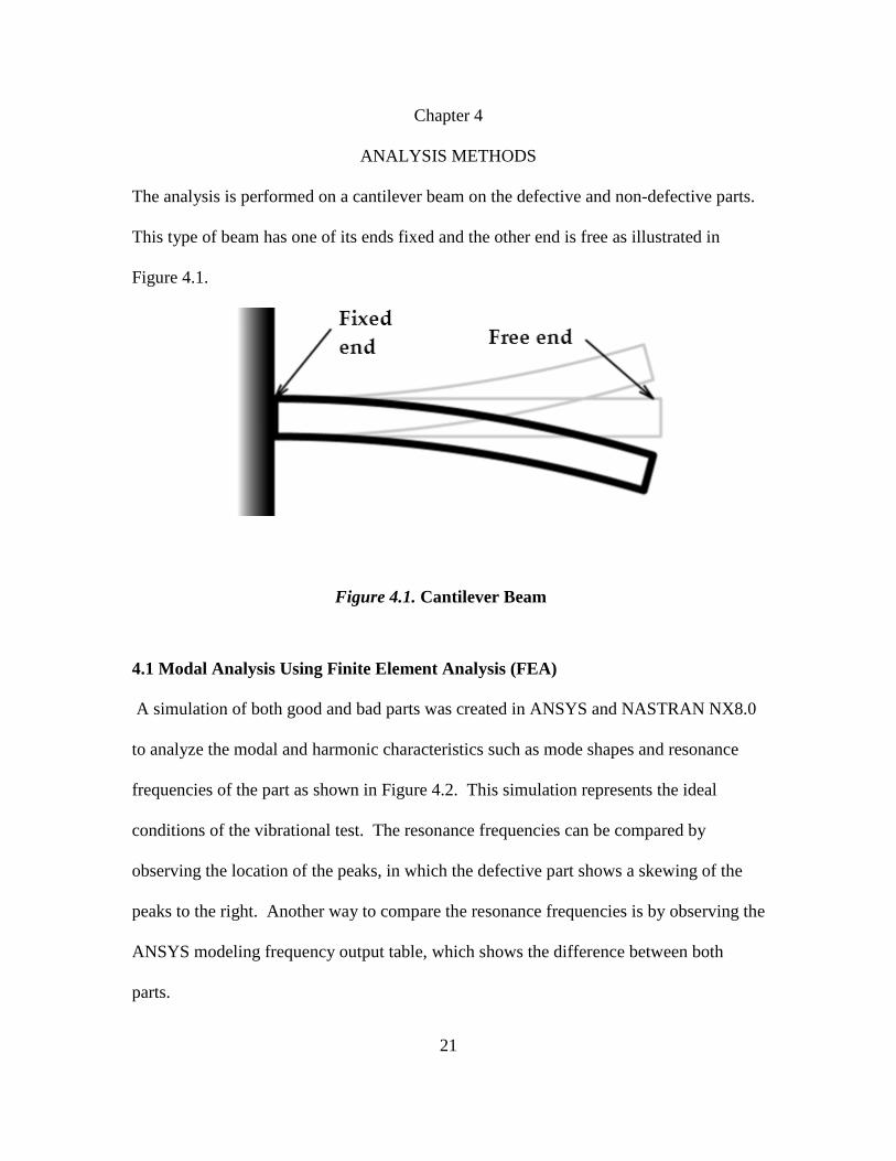
The analysis is performed on a cantilever beam on the defective and non-defective parts.
This type of beam has one of its ends fixed and the other end is free as illustrated in
Figure 4.1.
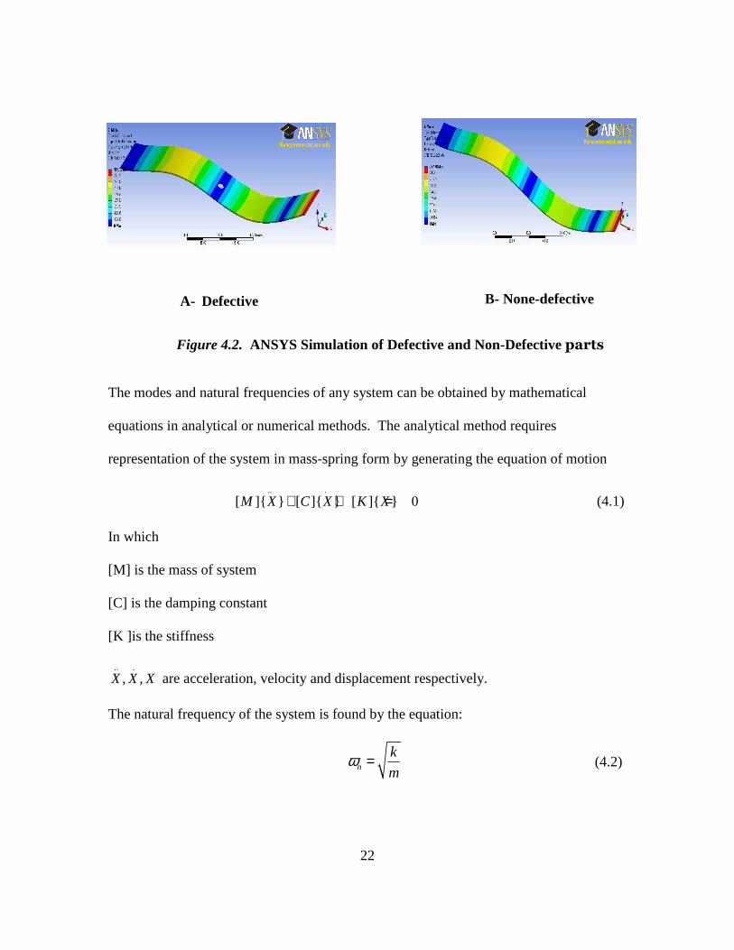
4.1 Modal Analysis Using Finite Element Analysis (FEA)
A simulation of both good and bad parts was created in ANSYS and NASTRAN NX8.0
to analyze the modal and harmonic characteristics such as mode shapes and resonance
frequencies of the part as shown in Figure 4.2. This simulation represents the ideal
conditions of the vibrational test. The resonance frequencies can be compared by
observing the location of the peaks, in which the defective part shows a skewing of the
peaks to the right. Another way to compare the resonance frequencies is by observing the
ANSYS modeling frequency output table, which shows the difference between both
parts.
Figure 4.1. Cantilever Beam
22
The modes and natural frequencies of any system can be obtained by mathematical
equations in analytical or numerical methods. The analytical method requires
representation of the system in mass-spring form by generating the equation of motion
.. .
[ ]{ } [ ]{ } [ ]{ } 0M X C X K X+ + = (4.1)
In which
[M] is the mass of system
[C] is the damping constant
[K ]is the stiffness
.. .
, ,X X X are acceleration, velocity and displacement respectively.
The natural frequency of the system is found by the equation:
n
k
mω = (4.2)
Figure 4.2. ANSYS Simulation of Defective and Non-Defective parts
A- Defective B- None-defective

23
The mode shapes and corresponding frequencies depend on the boundary conditions. In
this work, the samples are fixed from one side and free on the other side (cantilever beam).
The equation of motion of a cantilever beam:
2 2
2 2
( )[ ] ( ) ( )
n
d dY xEI m x Y x
dx dx ω= (4.3)
Where:
E is the modulus of elasticity
I is the moment of inertia
Y(x) is the displacement in Y-direction
nω is the natural frequency
Boundary conditions of a cantilever beam are:
0Y = at x=0, no deflection at the fixed end
0dY
dx= at x=0, no angular deflection at the fixed end
2
20
d Y
dx= at x=0 and x=L, no bending moment at the free end
3
30
d Y
dx= at x=L, no shear force at the free end
By applying the boundary conditions on the equation of motion of the cantilever beam,
the frequency equation can be obtained:
cos cosh 1n nL Lβ β+ = − (4.4)
Where 4β =2n m
EI
ω
Now the mode shapes equation can be obtained for a cantilever beam:

24
( ) [(sin sinh )(sin sinh ) (cos cosh )(cos cosh )]f x A L L x x L L x xβ β β β β β β β= − − + + −
(4.5)
Mode shapes and corresponding frequencies values depend on the material properties and
boundary conditions. For a cantilever beam these values are listed in Table 3.2.
Mode Natural frequency
First
43.515n
EI
ALω
ρ=
Second 4
22.03n
EI
ALω
ρ=
Third 4
61.7n
EI
ALω
ρ=
4.2 Mathematical Model
The model of each dynamical system represents the behavior and characteristics when a
specific input signal is applied, then depending on these characteristics, the system
responses with an output signal. In this work, many models in different forms are predicted
and evaluated using the experimental data. The time domain data of a non-defective part
is selected to perform this analysis. The predicted system models are used to calculate the
output ( )y t when a specific input signal ( )u t is applied. Input signal is a sine sweep of
0.01-5000 KHZ, half of the signal data is used to generate the model and the other half is
Table 4.1 Natural frequencies of first three modes

25
used for validation. The predicted models quality can be measured by a parameter called
Final Prediction Error (FPE), which is given by:
2
(1 )d
FPE VN
= + (4.6)
Where:
V is the loss function
d is number of estimated parameters
N is number of values of the data set
This parameter is used to compare the predicted models. The quality of models increases
when the FPE value is reduced.
The types of evaluated models are:
a. Autoregressive-moving average model with exogenous component (ARMAX)
It is a time series model used for simulating and predicting economics and industrial
behavior. This model was introduced by Wold (1938) as a combination of
Autoregressive and Moving average models (Makridakis & Hibon). The model
equation consists of multiple polynomials and it can be written as
Ay Bu Ce= + (4.7)
In MATLAB, the order of each polynomial is described and has a value which can be
adjusted to get the best model results.
an Order of the polynomial A(q)
bn Order of polynomial B(q)+1
cn Order of polynomial C(q)
kn Input-output delay

26
This model has been used to represent the relationship between the input and output
of a system (Fung, Wong, Ho, & Mignolet, 2003). The experimental time series data
(Time –Velocity) can be imported to MATLAB workspace, then a selection of
ARMAX model parameters can be done by iterations until the best model fit is
reached.
b. Box-Jenkins model (BJ)
It is a method uses time domain data to predict a system model. The method follows five
steps to select, identify and perform an assessment on conditional mean models
(Mathworks, n.d.). The steps of predicting the model are:
1. Keeping the time domain series stationary
2. Predicting the stationary for the data
3. Estimating the model parameters
4. Performing goodness fit checks to ensure the system is describing the
experimental data
5. Generating Monte Carlo simulations for the future time data
The equation of the model is
B C
y u eF D
= + (4.8)
During performing the model analysis in MATLAB, the order of each polynomial
must be estimated in order to get the best fit. The notation of each polynomial order are:
Order of B polynomial+1 bn
27
Order of C polynomial+1
dn Order of D polynomial+1
fn Order of F polynomial+1
Input delay
c. Output-error model (OE)
This model is generated when the disturbance is affecting the output signal (Jamil,
Sharkh, & Hussain, 2008). The output is represented as a function of the input and the
error.
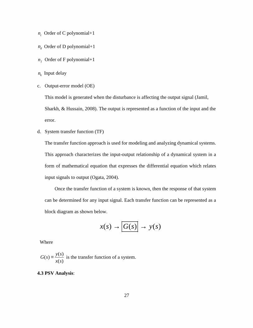
d. System transfer function (TF)
The transfer function approach is used for modeling and analyzing dynamical systems.
This approach characterizes the input-output relationship of a dynamical system in a
form of mathematical equation that expresses the differential equation which relates
input signals to output (Ogata, 2004).
Once the transfer function of a system is known, then the response of that system
can be determined for any input signal. Each transfer function can be represented as a
block diagram as shown below.
( ) ( ) ( )x s G s y s→ →
Where
( )
( )( )
y sG s
x s= is the transfer function of a system.
4.3 PSV Analysis:
cn
kn
28
The frequency domain data can be simulated in the PSV software to get the mode shapes
and amplitude peaks for both good and bad parts.
The response from the laser Vibrometer is in two forms, time domain and frequency
domain. In the time domain, the collected velocity data is varying during (1.27 seconds)
time period. While in frequency domain, the velocity is varying depending on the value
of the frequency. As it illustrated in Figure 3.5., the velocity response has some
amplitudes at certain frequencies. These amplitudes are generated at the resonance
frequency of the part.
4.4 Discriminant Analysis
It is a method used for classification when there is more than one group that differ in
some parameters’ values or types. This method is used to distinguish between these
groups. A fitting function is employed to create the class type from experimental training
data which is used to classify any data under investigation to recognize which group it is
belong to.
4.4.1 Purpose of discriminant analysis:
1. Creates a model that describes the difference between patterns with different
classes in terms of parameters
2. Predicts the class of unclassified testing data
4.4.2 Fisher Discriminant Analysis
It is a technique that produces a discriminant function to classify two types of data by
creating a projection on a line in such a way that samples are separated into their classes
(Bishop, 1995). This technique increases the difference of variance between the classes
with respect to the variance of data of each class. If n1, n2 are two samples for class1 and

29
class2 respectively then the projection iy of element ix in the w direction can be given
by the scalar dot product:
ty w x= (4.9)
In Fisher’s discriminant analysis both sample classes are projected on the line, the
difference between the means of the projected samples is used as a classification measure.
The mean of sample 1 and 2 are:
1
11
x D
X
nµ ∈=
∑ (4.10)
2
22
x D
X
nµ ∈=
∑ (4. 11)
Where 1D and 2D are data of group1 and 2 respectively.
Then the means of the projected samples are given by
� 1
1 11
t
x D t
w x
wn
µ µ∈= =∑
(4.12)
� 2
2 22
t
x D t
w x
wn
µ µ∈= =∑
(4.13)
Also the difference between the means is given by
� �1 2 1 1( )twµ µ µ µ− = − (4.14)
The scatter of the projected samples is
�
1 1 1
2 2 21 1 1 1 1( ) ( ) ( ) ( )t t t t
y P x D x D
s y w x w w x x wµ µ µ µ∈ ∈ ∈
= − = − = − −∑ ∑ ∑ɶ (4.15)

30
�
2 2 2
2 2 22 2 2 2 2( ) ( ) ( ) ( )t t t t
y P x D x D
s y w x w w x x wµ µ µ µ∈ ∈ ∈
= − = − = − −∑ ∑ ∑ɶ (4.16)
Where 1P and 2P are the projected data of both class samples.
In this discriminant analysis, the linear relationship between the original and the
projected data maximize the following criterion:
� � 2
1 22 21 2
( )( )J w
s s
µ µ−=+ɶ ɶ
(4.17)
Since this classification based on the direction of the projection line, thus it is necessary
to evaluate the criterion ( )J w as an explicit function ofw . The scatter matrices are
calculated in terms of the mean and the data of each sample and they can be written as:
1
1 1 1( )( )t
x D
S x xµ µ∈
= − −∑ (4.18)
2
2 2 2( )( )t
x D
S x xµ µ∈
= − −∑ (4.19)
The summation of both scatter matrices is given by
1 2wS S S= + (4.20)
Then equations (4.15) and (4.16) can be written as
21 1
ts w S w=ɶ (4.21)
22 2
ts w S w=ɶ (4.22)
Then
2 21 2 1 2 1 2( )t t ts s w S w w S w w S S w+ = + = +ɶ ɶ (4.23)
Substituting equation (4.20) leads to
2 21 2
tws s w S w+ =ɶ ɶ (4.24)

31
Similarly the numerator of equation (4.17) can be obtained in terms of w
� � 2 2
1 2 1 2( ) ( )t tw wµ µ µ µ− = − (4.25)
1 2 1 2( )( )tw wµ µ µ µ= − − (4.26)
Then simply ( )J w can be found as a function of w
( )t
Bt
w
w S wJ w
w S w= (4.27)
Where 1 2 1 2( )( )tBS µ µ µ µ= − −
For better classification results, the greater the difference between the projected samples
means the better the classification.
2
1 2
2 21 2
( )( ) p p
p p
J vs s
µ µ−=
+ (4.28)
The greater the difference between the projected means leads to more accurate
classification.
4.6 Neural Network
This classification method uses the input training data to generate an output classification
pattern. This method can be used to solve different types of problems by using some tools
such as fitting, pattern recognition, clustering, and time series tools. In this work, a neural
network is used to classify train the experimental data sets into two classes, then according
to the output classification, the classifier used to test any other sets of data. The network
consists of two layers, one is hidden and the second is the output neurons, the range of the
output signal is 0-1. In this analysis, a frequency-velocity data is imported in MATLAB.
This data contains data of ten non-defective and ten defective samples. Each sample has
32
6400 sampling rate, so the total of samples is 128,000 of either 0 or 1 output. The type of
the network is two-layer feed-forward with sigmoid hidden and output neurons, which
means that the input data information is moving in only one direction (forward) and it does
not have any loops. The network uses a back propagation in order to update the values of
bias and weights by estimating the gradient through the conjugant gradient method. The
fundamental principle of Neural Network is based on the values of the classified data, and
depending on the weight of the values, the class type is identified. The Network consists
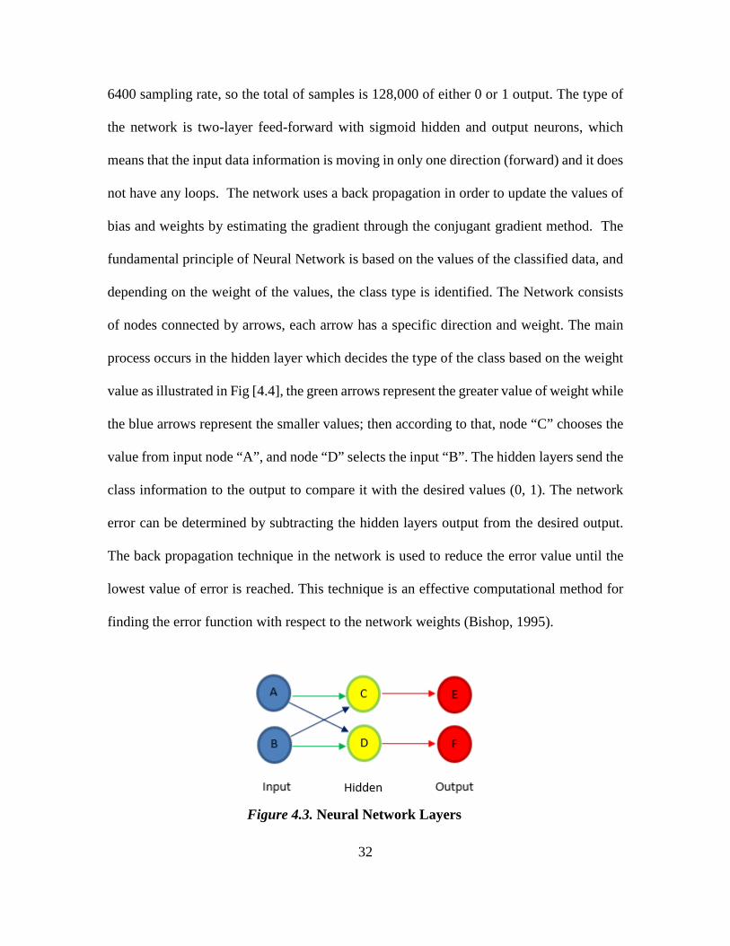
of nodes connected by arrows, each arrow has a specific direction and weight. The main
process occurs in the hidden layer which decides the type of the class based on the weight
value as illustrated in Fig [4.4], the green arrows represent the greater value of weight while
the blue arrows represent the smaller values; then according to that, node “C” chooses the
value from input node “A”, and node “D” selects the input “B”. The hidden layers send the
class information to the output to compare it with the desired values (0, 1). The network
error can be determined by subtracting the hidden layers output from the desired output.
The back propagation technique in the network is used to reduce the error value until the
lowest value of error is reached. This technique is an effective computational method for
finding the error function with respect to the network weights (Bishop, 1995).
Figure 4.3. Neural Network Layers

33
The network input and hidden layers contain bias values. The network in Fig 4.5.,
consists of input layer(x), hidden layer (z), and output layer (y). The weight can be
calculated by combining the bias of the jth hidden element (10jw ) with the weight of the
input layer ( 1ijw ) (Bishop, 1995), and it can be written as:
1 10
1
d
j ji i ji
a w x w=
= +∑ (4.29)
For simplicity, the bias term could be eliminated and equation (4.29) could be rewritten
as:
1
1
d
j ji ii
a w x=
=∑ (4.30)
A continuous sigmoidal function is used to activate the hidden unit ( jz ) which is
represented in equation (4.31)
( )j jz g a= (4.31)
Since this network contains two layers, the second layer is used to compute the
output. Then the output of the hidden units can be represented in the same way used in
the first layer
(2)
1
m
k kj ji
a w z=
=∑ (4.32)
In order to obtain the activation of the kth output, the linear equation (4.32) could be
transformed using a nonlinear function �(.)g (Bishop, 1995).
�( )k ky g a= (4.33)
The final network equation is written in the following form

34
� (2) (1)
0 0
( ( ))m d
k kj ji ij i
y g w g w x= =
= ∑ ∑ (4.34)
The percentage of well and misclassified data for training, testing, and validation is
estimated by a confusion matrix. The diagonal shows correct predictions, while the other
values show the incorrect prediction or the misclassified data.
Figure 4.5. Neural Network Design in MATLAB
Figure 4.4. Feed-Forward Network with Two Layers (Bishop, 1995)

35
The neural network toolbox in MATLAB splits the data into three groups training,
validation, and testing. The percentage of each group is selected by user and can be
adjusted to get better classification results. The training and validation groups affect the
training process by adjusting the error and the generalization of the network until the
generalization stops improving.
4.6 Hilbert Huang Transform
Hilbert Huang Transform (HHT) is an algorithm uses non-linear non-stationary time
domain signal such as white noise wave to obtain the frequency output. This algorithm
decomposes the signal into intrinsic mode functions (IMF) which are a simple oscillatory
harmonic functions having the same number of highest amplitudes (extrema) and zero
Figure 4.6. Confusion Matrix

36
crossing and it can be described on x-y graph by variable amplitudes on the y-axis and
frequency along the x-axis. There are two steps to follow in order to use HHT algorithm:
1. Empirical mode decomposition (EMD)
2. Hilbert spectral analysis
The EMD is used to convert the non- linear time domain data into IMF. A process
called sifting is applied to find the IMF from given data. During this process, the local
upper amplitudes and lower amplitudes of the time data are evaluated, then these
amplitudes are connected by a spline line to create the upper and lower envelopes. The
average of these envelopes represent the frequency component which is then subtracted
from the original signal (Kim & Oh, 2009).
Figure 4.7. Sifting Process (Kim & Oh, 2009)
37
The Hilbert spectral analysis used for evaluating the instantaneous frequency of IMF.
When the time domain signal ( )x t which includes a velocity changes over time is non-
stationary, then the evaluated analytic signal ( )z t is given by
( ) (t) i (t)z t x y= + (4.35)
Where ( )y t represents HHT of ( )x t and it is given by
1 ( )
( )x s
y t p dst sπ
∞
−∞
=−∫ (4.36)
p is the Cauchy principle value. The polar equation of the analytic signal ( )z t is
( ) ( )exp( ( ))z t a t i tθ= (4.37)
Here, ( )a t is the amplitude or called the envelope function (Hui & Zhang, 2009) and can
be written as 2 2( ) ( )x t y t+ , and ( )tθ is the phase which is given by ( )
arctan( )( )
y t
x t. The
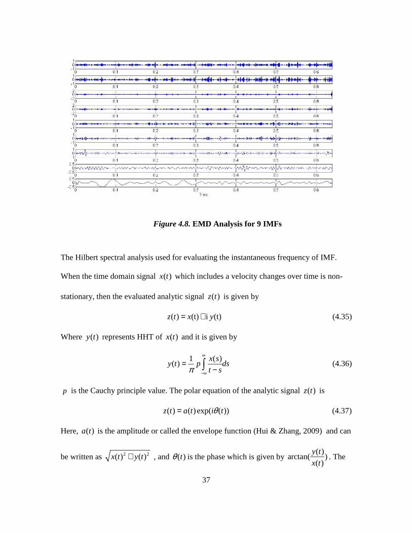
Figure 4.8. EMD Analysis for 9 IMFs
38
instantaneous frequency w is the time derivative of the phase, it is written as ( )d t
dt
θ and
it is showing in Figure 4.10., as amplitudes and instantaneous frequency. The Hilbert
Huang Spectrum can be expressed as a function of time and frequency
1
( , ) ( )exp( ( ) )n
i ii
H t w r a t w t dt=
= ∑ (4.38)
In equation (4.38), r is the residue (Hui & Zhang, 2009). The Local Marginal Spectrum
of the IMF function is given by
0
( , )T
i ih H t w dt= ∫ (4.39)
Once the decomposition process is applied, the decomposed Time-Velocity signal of
each Empirical mode will have an envelope function and phase. The summation of the
Empirical modes leads to the original signal( )x t .
1
( ) ( )n
ix t E t=∑ (4.40)
Where
( )iE t The Empirical mode function
n Total number of Empirical modes
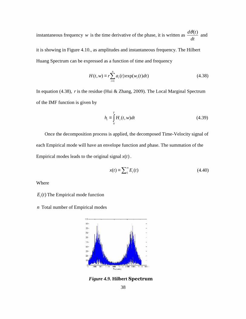
Figure 4.9. Hilbert Spectrum

39
Chapter 5
RESULTS
In this chapter, the techniques presented in chapter four are used for classification on the
same dataset. The data was obtained via PSV Laser Vibrometer setup discussed in chapter
three.
5.1 System Model
The model of the system can be identified and simulated in MATLAB by using the
(velocity-time) data, and according to the relationship between the input and the output,
the parameters of each model can be estimated to get the best model fit. In MATLAB
there are many suggested models can be performed on any set of data using the system
identification toolbox, and the final results of the simulation can be plotted over the
experimental graph in order to observe the accuracy of each system. The main purpose
of estimating the model for the none-defective parts is to generate an ideal model that
represents the good parts, then from any collected data from other samples can be used to
compare response with the ideal case. In this section, the ideal model was predicted and
generated using the non-defective sample. The experimental data was collected under
vibrational conditions of a sinusoidal sweep of (0.1-5) KHZ and the response was
collected using the Laser Scanning Vibrometer.
5.1.1 Autoregressive-moving average model (ARMAX)
The predicted model here is a combination of Autoregressive and Moving average
models with exogenous component. The parameters where found using trial and error
40
method in order to get the best fit compared to experimental data graph. Equation (4.7)
represents ARMAX model and can be written as a function of time
( ) ( ) ( ) ( ) ( ) ( )A q y t B q u t C q e t= + (5.1)
1 2 3 4( ) 1 3.42 4.784 3.307 0.9436A q q q q q− − − −= − + − +
1 2 3( ) 2404 4808 2404B q q q q− − −= + −
1 2 3 4 5 6( ) 1 2.472 2.483 0.9719 0.1973 0.3028 0.1448C q q q q q q q− − − − − −= − + − − + −
Loss function: 0.0111811
FPE: 0.0112166
Sampling interval: 7.8125e-005
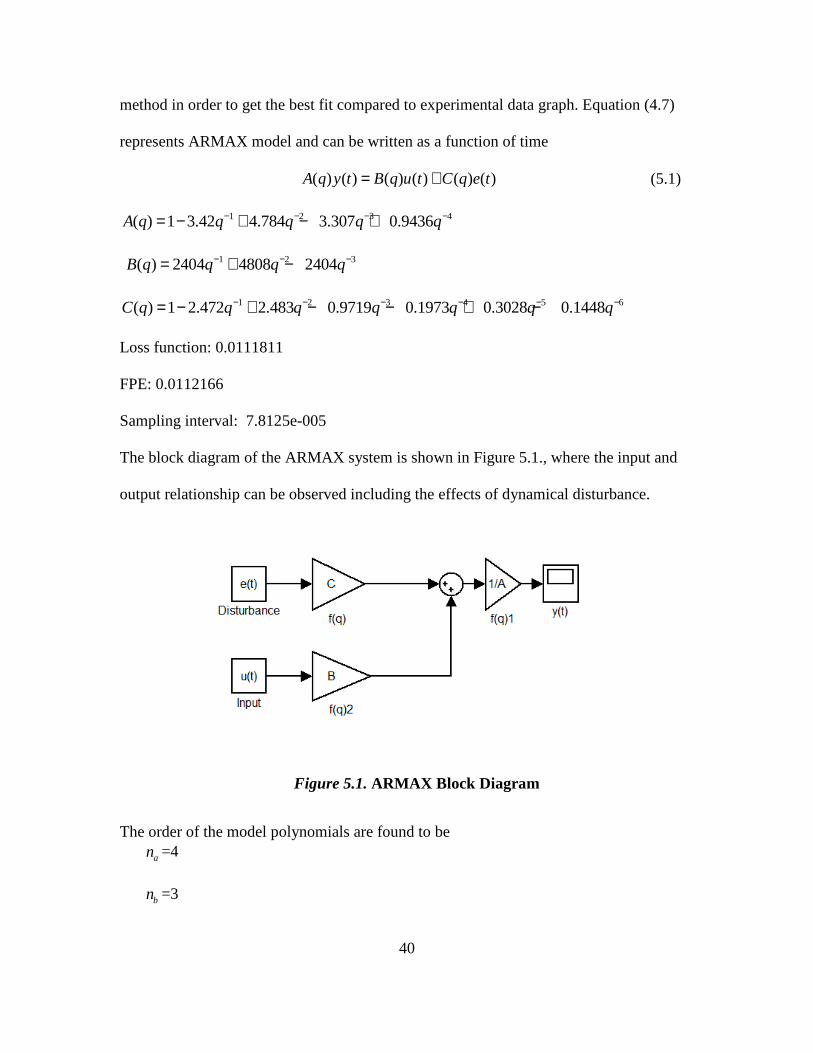
The block diagram of the ARMAX system is shown in Figure 5.1., where the input and
output relationship can be observed including the effects of dynamical disturbance.
The order of the model polynomials are found to be
=4
=3
an
bn
Figure 5.1. ARMAX Block Diagram

41
=6
=1
The ARMAX system model is shown in Figure 5.3., plotted on top of the experimental
data graph. From the output figure, it can be concluded that the model has a good fit and
it represents the true model as a combination of autoregressive-moving averages models.
cn
kn
Figure 5.2. ARMAX Parameters Setting
42
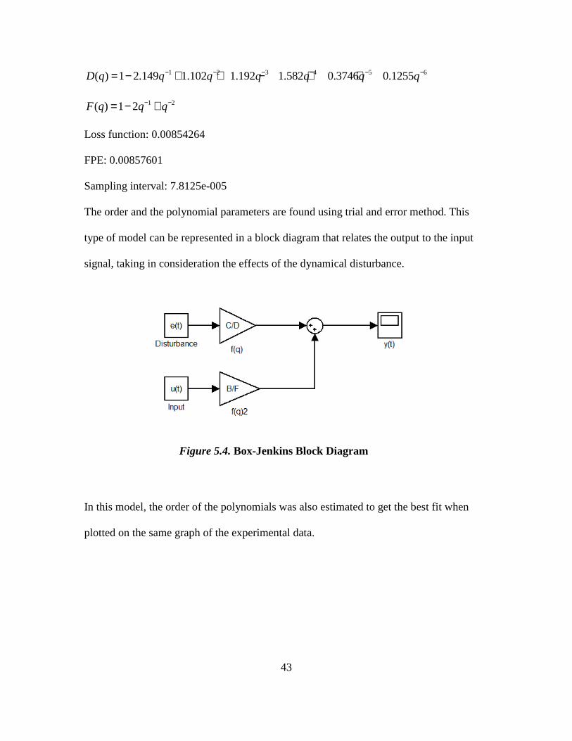
5.1.2 Box-Jenkins model
The general form of this of this model can be written as a mathematical equation that
relates the output to the input signals that changes with time. Equation (5.2) shows the
model input-output relationship:
( ) ( )
( ) ( ) ( )( ) ( )
B q C qy t u t e t
F q D q= + (5.2)
4 5 6 7( ) 6786 2002 2.436 004 1.557 004B q q q e q e q− − − −= − − + −
1 2 3 4( ) 1 1.396 0.08773 1.225 0.8028C q q q q q− − − −= − + +
Figure 5.3. ARMAX Model
43
1 2 3 4 5 6( ) 1 2.149 1.102 1.192 1.582 0.3746 0.1255D q q q q q q q− − − − − −= − + + − + +
1 2( ) 1 2F q q q− −= − +
Loss function: 0.00854264
FPE: 0.00857601
Sampling interval: 7.8125e-005
The order and the polynomial parameters are found using trial and error method. This
type of model can be represented in a block diagram that relates the output to the input
signal, taking in consideration the effects of the dynamical disturbance.
In this model, the order of the polynomials was also estimated to get the best fit when
plotted on the same graph of the experimental data.
Figure 5.4. Box-Jenkins Block Diagram

44
The model output shows a good response and an accurate fit to the original experimental
data.
Figure 5.6. Box-Jenkins Model
Figure 5.5. Box-Jenkins Parameters Setting
45
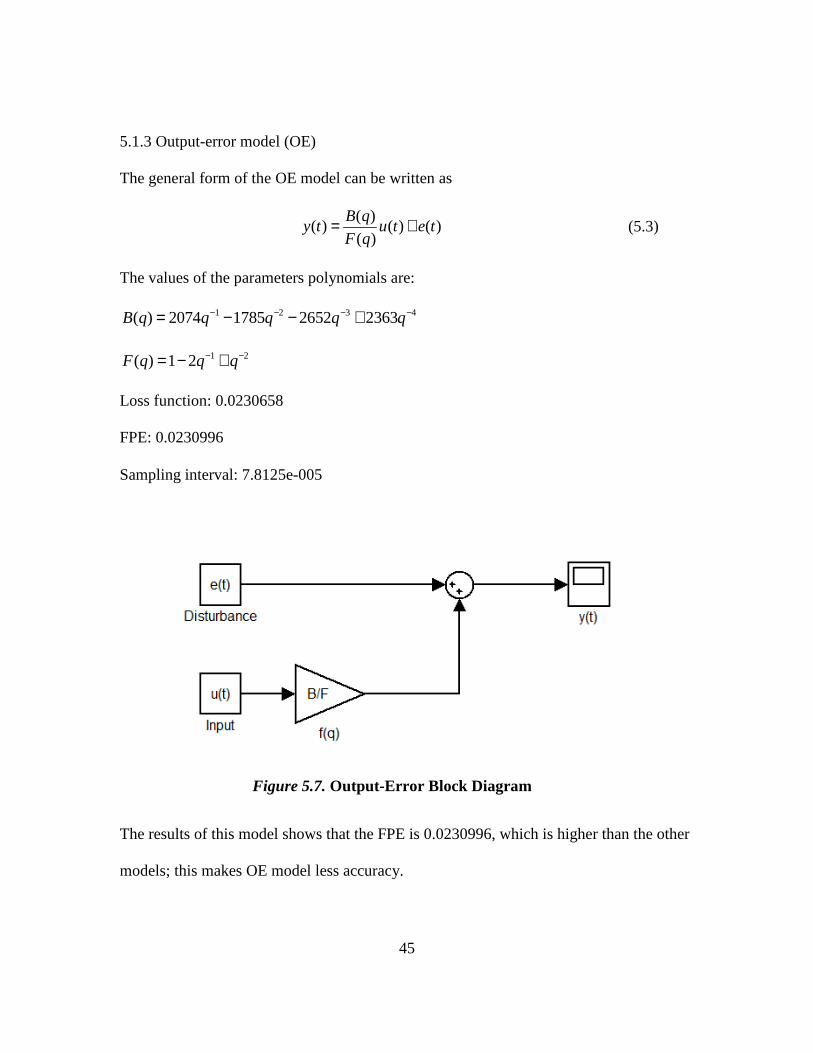
5.1.3 Output-error model (OE)
The general form of the OE model can be written as
( )
( ) ( ) ( )( )
B qy t u t e t
F q= + (5.3)
The values of the parameters polynomials are:
1 2 3 4( ) 2074 1785 2652 2363B q q q q q− − − −= − − +
1 2( ) 1 2F q q q− −= − +
Loss function: 0.0230658
FPE: 0.0230996
Sampling interval: 7.8125e-005
The results of this model shows that the FPE is 0.0230996, which is higher than the other
models; this makes OE model less accuracy.
Figure 5.7. Output-Error Block Diagram

46
The parameters were computed in MATLAB, also the order of the polynomials were
estimated using trial and error.
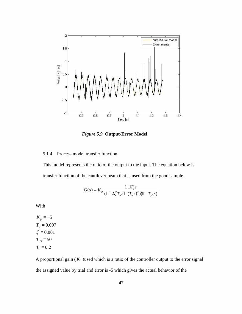
Figure 5.9 shows the estimated parameters which are selected by trial and error until best
fit is reached. The output of the model is plotted over the experimental data, as it can be
seen that the model has a good fit in approximating the system model.
Figure 5.8. Output-Error Parameters Setting
47
5.1.4 Process model transfer function
This model represents the ratio of the output to the input. The equation below is
transfer function of the cantilever beam that is used from the good sample.
2
3
1( )
(1 2 ( ) )(1 )z
pw w p
T sG s K
T s T s T sζ+=
+ + +
With
3
5
0.007
0.001
50
0.2
p
w
p
z
K
T
T
T
ζ
= −
==
=
=
A proportional gain ( Kp )used which is a ratio of the controller output to the error signal
the assigned value by trial and error is -5 which gives the actual behavior of the
Figure 5.9. Output-Error Model

48
relationship between the time and velocity; moreover, increasing the time reduces the
velocity amplitudes. The damping ratio is <1 which makes the system under damped,
which also represents the real case of a cantilever beam vibration.
The model has 1 zero and 3 poles and an integrator. The zero time constant (Tz), the time
constant of the complex poles (TW), and the time constant of real poles (Tp3) were
estimated to get the best accurate results.
Figure 5.10. Open-Loop Transfer Function
Figure 5.11. Process Model

49
5.2 Fisher Discriminant Analysis
This analysis was performed using 10 non-defective samples and 10 defective
samples at 6400 sampling rate which leads to using 128,000 values of frequency-
velocity data. In the final results, the output graph contains a curve that shows the
class of any unknown data of a sample under same vibrational conditions.
The graph of Figure 5.13., represents the non-defective part, where most of the
amplitudes are below the classification curve.
Figure 5.12. Fisher Non-Defective Sample

50
The defective part graph shows higher amplitudes that passes the classification line as
well as some of the amplitudes reaches the the top left corner of the graph.
5.3 Neural Network Classification
The Neural network classification is performed in order to get the class output of any
imported unknown sample. Once the classification is done, validation takes action to
assure that the classification is accurate then a small percentage from the classification
data is used for testing the classifier. The accuracy of all these classifier building stages is
shown in the confusion matrix, as illustrated in Figure 5.15.
Figure 5.13. Fisher Defective Sample

51
The diagonal of each matrix represents the accurate percentage of the data and the
total good percentage is located in the blue cells, while the red cells represent the
misclassified percentage. As shown in the matrices that the total percentage of the
training data is 78.3%, the validation is 78.4%, the testing is 77.6%, and the overall
percentage is 78.2%.
Figure 5.14 Confusion Matrix of NN Classifier
52
The accuracy of the classifier did not reach the 100% because of the large number -
128,000 experimental training data of non-defective and defective samples.
Once the training process is done, the classifier is ready for testing any unknown data
that is collected under the same vibrational conditions of the classification data. Table
5.1 shows the results of testing 10 samples, the class of each sample is on the right
side of the table. The Neural Network results is represented in a matrix form. In this
analysis the difference in the third column which represents the average values of the
output is used to recognize the class of data; if the output number of any data under
investigation in the third column is < 0.34 then the sample is non-defective. On the
other hand, if the value is> 0.34 then the sample considered as a defective.
Sample Output1 Output2 Type 1 0.6717 0.3264 Good 2 0.6705 0.3275 Good 3 0.6649 0.3331 Good 4 0.6692 0.3289 Good 5 0.6989 0.2993 Good 6 0.3158 0.6796 Bad 7 0.3055 0.6897 Bad 8 0.3055 0.6897 Bad 9 0.2969 0.6983 Bad 10 0.2996 0.6956 Bad
The dotted line in Figure 5.16 represent the best validation, while the colored lines are the
classification data. It can be noticed that the classifier did not match the best fit because
of the type of data in which many values are the same for defective and non-defective
samples. The Mean Squared Error (MSE) is the difference between actual and desired
Table 5.1. Neural Network results

53
output. The accuracy of the classifier increases when MSE has least value. The values of
MSE for best fit is found to be 0.15493 at epoch 383.
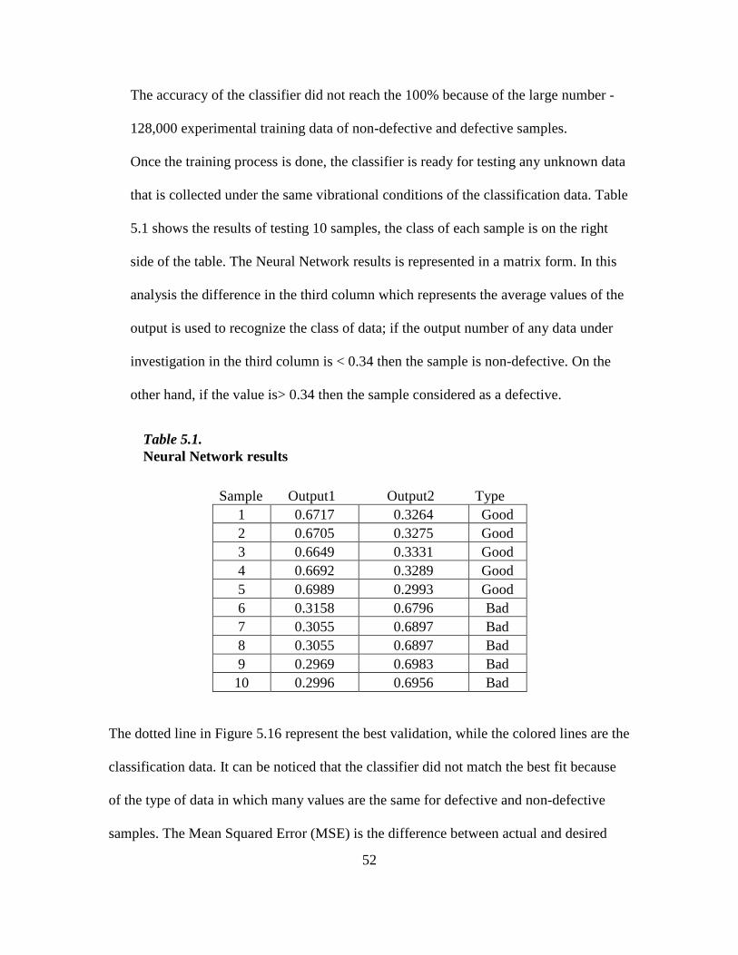
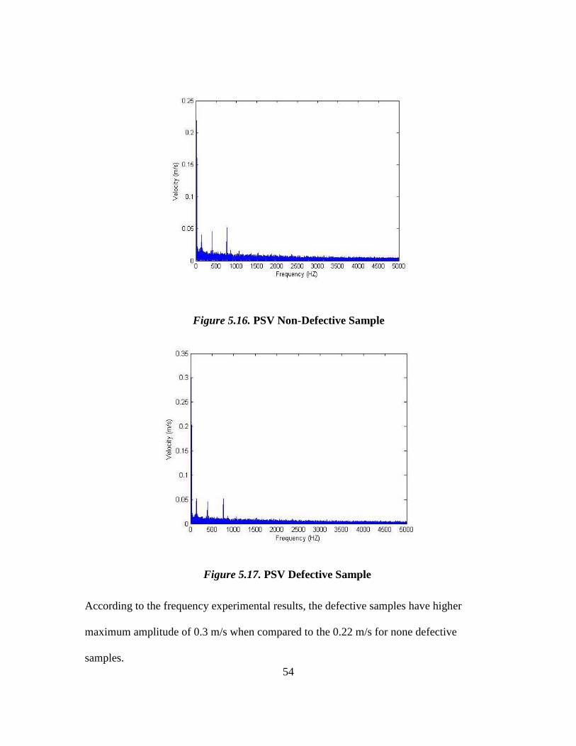
5.4 PSV Frequency Domain Comparison
From the PSV output analyzer for both good and bad samples, a difference could be
obtained by observing the location and the values of the peaks.
The data was collected for many samples under different vibrational frequencies and
sampling rates. The test was performed on 8 samples at 6400 sampling rate using white
noise wave at frequency of 1-5000 HZ. The figures below show the difference between
the good and bad under same vibrational conditions. From graphs, at low frequencies the
amplitudes of the defective parts have higher values under the same testing conditions.
Figure 5.15. NN Classification Accuracy
54
According to the frequency experimental results, the defective samples have higher
maximum amplitude of 0.3 m/s when compared to the 0.22 m/s for none defective
samples.
Figure 5.16. PSV Non-Defective Sample
Figure 5.17. PSV Defective Sample
55
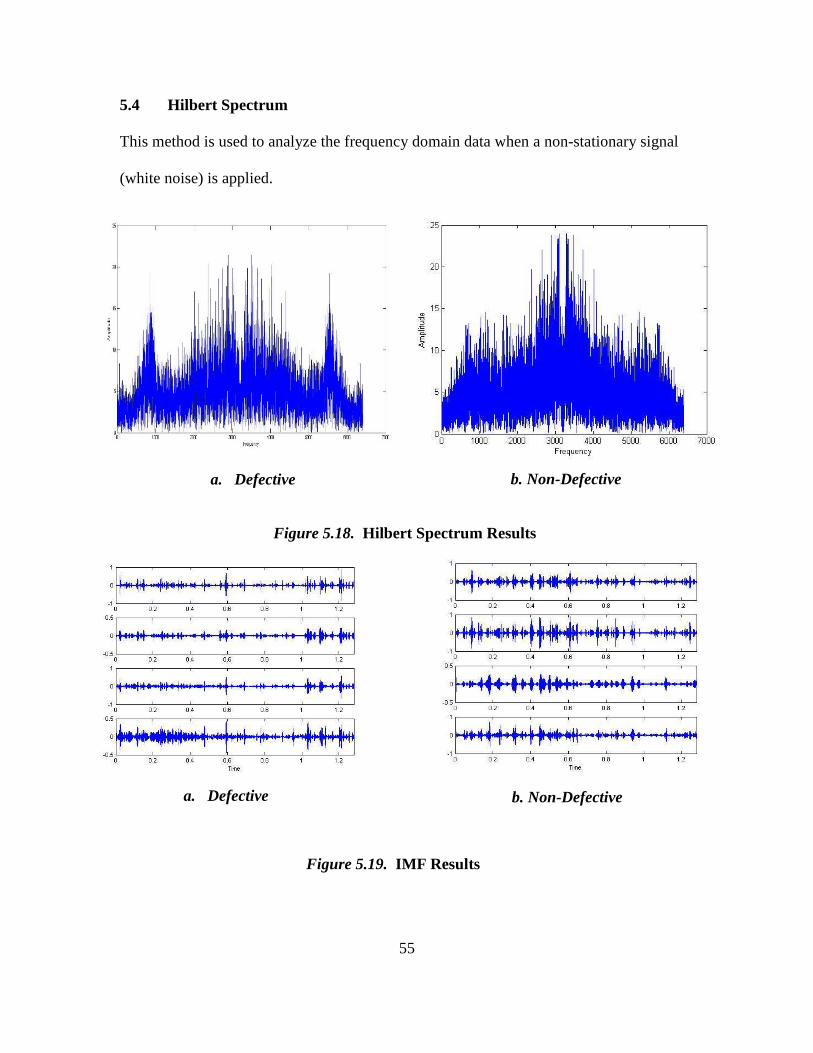
5.4 Hilbert Spectrum
This method is used to analyze the frequency domain data when a non-stationary signal
(white noise) is applied.
Figure 5.18. Hilbert Spectrum Results
b. Non-Defective a. Defective
Figure 5.19. IMF Results
b. Non-Defective a. Defective
56
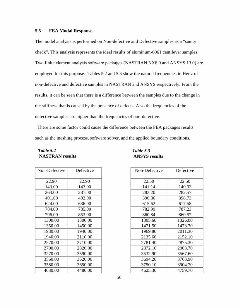
5.5 FEA Modal Response
The model analysis is performed on Non-defective and Defective samples as a “sanity
check”. This analysis represents the ideal results of aluminum-6061 cantilever samples.
Two finite element analysis software packages (NASTRAN NX8.0 and ANSYS 13.0) are
employed for this purpose. Tables 5.2 and 5.3 show the natural frequencies in Hertz of
non-defective and defective samples in NASTRAN and ANSYS respectively. From the
results, it can be seen that there is a difference between the samples due to the change in
the stiffness that is caused by the presence of defects. Also the frequencies of the
defective samples are higher than the frequencies of non-defective.
There are some factor could cause the difference between the FEA packages results
such as the meshing process, software solver, and the applied boundary conditions.
Non-Defective Defective Non-Defective Defective
22.90 22.90 22.50 22.50 143.00 143.00 141.14 140.93 263.00 281.00 283.20 282.57 401.00 402.00 396.86 398.73 624.00 636.00 615.62 617.58 784.00 785.00 782.99 787.23 796.00 853.00 860.84 860.57 1300.00 1300.00 1305.60 1326.00 1350.00 1450.00 1471.50 1473.70 1930.00 1940.00 1969.80 2011.30 1940.00 2110.00 2135.60 2152.10 2570.00 2710.00 2781.40 2875.30 2700.00 2820.00 2872.10 2903.70 3270.00 3590.00 3532.90 3567.60 3560.00 3620.00 3694.20 3763.90 3580.00 3650.00 3750.10 3904.70 4030.00 4480.00 4625.30 4759.70
Table 5.2 NASTRAN results
Table 5.3 ANSYS results

57
4550.00 4620.00 4873.20 5153.90 4870.00 5450.00 5674.70 5877.10
As shown in the ANSYS results that at low frequencies the non-defective parts have a
slightly higher values; this is normally happen because the defects are identified at higher
frequencies.

58
Chapter 6
CONCLUSION
The thesis’s main objective was to study the methodologies for NDT using a resonance
testing technique. The testing was performed using a high accuracy Laser Scanner
Vibrometer which generate vibrational signals and acquire data in time and frequency
domain at the same time. To achieve the successful identification/classification, several
pattern recognition, FEA simulation, and system modeling methods were applied. Some
of these methods used time domain data and others uses frequency domain data and.
Based on the analysis and results of each method, it can be noted that-
1. Performing the test in two domains increased the effectiveness of the identification
process, so if some of the defect signals were not detected in one domain, then they
could be identified in the other domain.
2. The Modal analysis in ANSYS and NASTRAN NX8.0 represented the ideal case of
defective and non-defective samples. This analysis provides all the information of the
natural frequencies and it shows how the values were changing due to the presence of
the defects especially at high frequency range. There was a small difference between
the results by ANSYS and NASTRAN NX8.0 that could be attributed to the variation
in number of the elements, mesh accuracy, and the software solver environment.
3. Fisher’s discriminant analysis showed effective results by creating a classification
border to separate the majority of data values above or under the border. As described
in sections [4.5.2] and [5.2]. The output of the classifier had two values, each one
represents a class type. In addition, the defective samples showed higher amplitude
values and then can be identified easily.

59
4. Neural Network can be successfully used to identify the class of testing data.
However, data training should take place first for generating the class. Second, a
validation process should be carried out. Once the training and testing is done to
detect the accuracy of classifier on a sample dataset, a testing process should be
performed on the actual dataset. The classification results showed the significant
difference in the sample’s output.
5. The Hilbert Huang Transform (HHT) provided promising results for the time domain
data, and then represented it as a frequency spectrum at each IMF. The energy of the
spectrum of the none-defective samples is concentrated at 3000 Hz, while for the
defective it is at lower frequency value. As illustrated in Figure 5.18, the spread of the
amplitudes are different and the defective parts can be easily detected.
6. For the system identification approach, three system Models were predicted using
time domain data. Each model described the dynamical behavior of the non-defective
samples. The construction of system models was reached by estimating the model’s
parameters. Based on the final prediction error (FPE) value, the model was selected.
The less the value of FPE, led to the best fit model. In this analysis, the Box-Jenkins
model showed the least value of (FPE) which is 0.00857601. According to FPE, this
model considered as a best fit model to the experimental data that can describe the
system dynamical behavior.
7. Estimating the Transfer Function (TF) of any dynamical system is very important
because it determines the relationship between the input and the response of the
system. The experimental data and the transfer function showed that the system was

60
under damped and it has a damping ratio<1. The transfer function contained 1 zero
and 2 poles.
Based on the results analysis, Neural Network Method seems to have better output than
the other methods. The output of the classifier consists of numbers, percentage of well
and miss classified data. The difference between the output number of good and bad has
an easy criterion of classifying the part as defective or non-defective.
Finally, the Laser Scanning Vibrometer combined with pattern recognition was a
successful approach in identifying the defected parts with visible and invisible flaws.
This combination could add a crucial advantages to the product’s quality control.
The future work could include using a micro laser Scanning Vibrometer which is able to
detect micro defects and surface flatness. Moreover, a higher frequency vibration is
recommended by using the highest range of the scanner (30MHz) in order to get more
different amplitudes between the defective and non-defective samples. This
recommendation requires a higher frequency range shaker. For better results, it is
recommended to use higher quality holding fixture for the samples to represent the ideal
cantilever boundary conditions.
61
REFERENCES
Bishop, C. M. (1995). Neural Networks for pattern Recognition. Oxford: CLARENDON PRESS .
Breaban, F., Carlescu, V., Olaro, D., & Gh. Prisacaru, J. C. (2011). Laser Scanning Vibrometry Applied to Non-Destructive Testing of Electro-Acive Polymers. U.P.B. Sci. Bull.
Fung, E. H., Wong, Y., Ho, H., & Mignolet, M. P. (2003). Modelling and prediction of machining errors using ARMAX and NARMAX structures. Applied Mathematical Modeling.
Hui, L., & Zhang, Y. (2009). Hilbert-Huang transform and marginal spectrum for detection and diagnosis of localized defects in roller bearings. Journal of Mechanical Science and Technology 23, 291-301.
Huke, P., Focke, O., Falldorf, C., Kopylow, C. v., & Bergmann, R. B. (2010). Contactless Defect Detection Using Optical Methods for Non Destructive Testing. NDT in Aerospace, 8.
Huynh, D., & Tran, D. (2004). A Non-Destructive Crack Detection Technique Using Vibration Tests. Structural Integrity and Fracture.
IAEA. (2001). Guidebook for the Fabrication of Non-Destructive Testing (NDT) Test Specimens. Vienna: International Atomic Energy.
Jamil, M., Sharkh, S. M., & Hussain, B. (2008). Identification of Dynamic Systems & Selection. In J. M. Arreguin, Automation and Robotics (pp. 121-142). Rijeka: I-Tech Education and Publishing.
Kim, D., & Oh, H.-S. (2009). EMD: A Package for Empirical Mode Decomposition and Hilbert Spectrum. The R Journal , 40-46.
Li, H., Zhang, Y., & Zheng, H. (n.d.). Hilbert-Huang Transform and Marginal Spectrum for detection and diagnosis of localized defects in roller bearings.
Makridakis, S., & Hibon, M. (n.d.). ARMA Models and the Box Jenkins Methodology. Fontainebleau: INSEAD.
Mathworks. (n.d.). MATLAB. Retrieved from http://www.mathworks.com/help/econ/box-jenkins-model-selection.html
Ogata, K. (2004). System Dynamics. Upper Saddle River: Pearson Education, Inc.

62
Polytec. (n.d.). Hardware Manual Polytec Scanning Vibrometer PSV 300. Retrieved from University Of Cambridge: http://www-mech.eng.cam.ac.uk/dynvib/lab_facilities/vibrometer_hardware_manual.pdf
Price, T. L., Dalley, G., McCullough, P. C., & Choquette, L. (1997). Manufacturing Advanced Composite Components for Airframes. National Technical Information Service.
Santulli, C., & Jeronimidis, G. (2006). DEVELOPMENT OF A METHOD FOR NONDESTRUCTIVE TESTING OF FRUITS USING SCANNING LASER VIBROMETRY (SLV). Jornal of NDT, 12.
Schwarz, B. J., & Richardson, M. H. (1999). Experimental Modal Analysis. CSI Reliability Week. Orlando .
Smith, R. R., Callahan, N., & Strong, S. (2005). Developing a Practical Quality System to Improve Visual Inspections. Industrial Technology, 1-7.
Subramanian, D. (2013). Analysis of Resonance Testing Methodology for Characterization of Parts. Arizona State University.
Traynor, R. (n.d.). Non-Contact Vibration Measurement of Micro-Structures. Retrieved from Lambda Photometric: http://www.lambdaphoto.co.uk/pdfs/DMAC%20Talk%20Warwick%20Uni%208-4-03.pdf
Vanlanduit, S., Guillaume, P., Schoukens, J., & Parloo, E. (2006). Linear and Nonlinear Damage Detection Using a Scanning Laser Vibrometer. Brussel.
Vanlanduit, S., Parloo, E., & Guillaume, P. (n.d.). A Robust Singular Value Decomposition to Detect Damage Under Changing Operating Conditions and Structural Uncertainties. Brussels.
Wong, F., & Toppings, B. H. (1988). Finite Element Studies For Non-Destructive Vibration Tests. Comuter and Structures, 653-669.
Yang, S., & Allen, M. (2012). Output-onlyModalAnalysisusingContinuous-ScanLaserDoppler Vibrometryandapplicationtoa20kWwindturbine. Mechanical SystemsandSignalProcessing.
