at SciVerse ScienceDirect

Energy 44 (2012) 820e829

Contents lists available

Energy

journal homepage: www.elsevier .com/locate/energy

Non-dimensional scaling of tidal stream turbines

A. Mason-Jones a, D.M. O’Doherty a,*, C.E. Morris a, T. O’Doherty a, C.B. Byrne a, P.W. Prickett a,R.I. Grosvenor a, I. Owen b, S. Tedds b, R.J. Poole b

a School of Engineering, Queen’s Buildings, Cardiff University, The Parade, Cardiff, CF24 3AA, UKb School of Engineering, University of Liverpool, UK

a r t i c l e i n f o

Article history:Received 21 November 2011Received in revised form4 May 2012Accepted 7 May 2012Available online 10 June 2012

Keywords:Marine turbinesScalingCFDTorque coefficientPower coefficientThrust coefficientVelocity profile

* Corresponding author. Tel.: þ44 0 29 2087 4542;E-mail address: odohertydm@cf.ac.uk (D.M. O’Doh

0360-5442/$ e see front matter � 2012 Elsevier Ltd.doi:10.1016/j.energy.2012.05.010

a b s t r a c t

The impact of local depth-wise velocity profiles on tidal turbine performance is important. Although theuse of standard power laws for predicting velocity profiles is common, these laws may underestimate themagnitude of the depth-wise velocity shear and power attenuation. Predicting the performance of a tidalturbine in a high velocity shear is crucial in terms of power extraction. This paper discusses thedimensional scaling of a turbine using CFD and experimental data. Key performance characteristics(power, torque and thrust coefficients) were studies with increasing diameters and velocities, bygenerating. a series of non-dimensional curves. This provides a first order approximation for matchingturbine performance characteristics to site conditions. The paper also shows that the use of a volume-averaged velocity derived from the upstream velocity profile can be used to determine these keyperformance characteristics. These are within 2% of those determined assuming a uniform flow. Thepaper also shows that even changes in the blade pitch angle results in new turbine characteristics underuniform velocity conditions and it is expected that these can be used for profiled flow.

� 2012 Elsevier Ltd. All rights reserved.

1. Introduction

Tidal stream technology is now developing apace, differentturbine designs are being proposed, and experimental performancetesting is being carried out at small scale [1,2], with additionalsupport from Computational Fluid Dynamics (CFD) [3,4]. As with allmodel testing in fluid mechanics, there is the issue of how totranslate the results from the experimental to the full scale. Thescaling is conventionally done using non-dimensional analysis, andthe purpose of this paper is to demonstrate the effectiveness ofsuch an analysis when applied to a Horizontal Axis Tidal StreamTurbine (HATT) with a particular emphasis on how to deal with thecharacteristic velocity when the turbine is exposed to a non-uniform inlet velocity profile.

When deploying HATTs, it was suggested over a decade ago byBryden et al. [5] that where shipping restrictions exist, the tip of therotor needs to be 1.5m below the lowest astronomical tide (LAT) forthe lowest negative storm surge, another 2.5 m for the trough ofa 5 mwave and a further 5 m to minimise the potential for damagefrom local shipping lanes. Therefore, the tip of a HATT at top deadcentre should be around 9 m below LAT. It has also been recom-mended that the bottom of the HATT should not be within 25% of

fax: þ44 0 29 2087 4597.erty).

All rights reserved.

the water depth at LAT from the seabed due to the high shear levelsat these depths [6]. However this 25% restriction on the distancebetween the seabed and rotor tip may not be practical at locationswhere large cargo vessels are common place, such as within theSevern Estuary where vessel drafts of approximately 14 m aretypical and the maximum available depth is 35 m [7].

Although the Severn Estuary is not currently one of the primesites for deploying tidal stream turbines, it may be an importantpart of the UK’s tidal stream resource in the future, due to its abilityto mitigate problems associated with power variability from out ofphase tidal cycles and power variability. In fact, it has been shownthat with the installation of tidal stream devices located in theSevern Estuary along with further installations in the Clyde, Tees,Humber, Menai Straits and the Mersey, a regular National gridsupply could be established [8].

The DTI report on the economic viability of a simple tidal streamenergy capture device [9], and UK resource estimates from Blackand Veatch [10] suggest that typical water depths at the suitablesites around the UK range from 25 to 40 m and that consequentlythe corresponding recommended rotor diameter is between 10 mand 20 m. However, as device deployment expands into largearrays, additional placement restrictions from local water depthsand/or shipping may arise. As such, it is likely that some turbineswill need to be placed within 25% of the water depth at LAT fromthe seabed to maximise the power generated.

Nomenclature

A swept area of the turbine (m2)CP power coefficientCT thrust coefficientCq torque coefficientD diameter (m)F axial thrust or force generated (N)H height from seabed to turbine rotational centre (m)HATT horizontal axis tidal turbineP power generated (W)R radius of turbine (m)Re Reynolds numberRSM Reynolds Stress Model

T torque generated by the flow (Nm)TSR tip speed ratiounc uncorrected performance characteristicUF unbounded free stream velocity in the water flume

(m/s)UT free stream velocity in the water flume (m/s)UT/UF blockage correction factorV velocity (m/s)Vd depth-averaged velocity (m/s)Vv volume-averaged velocity (m/s)r density (kg/m3)u angular velocity (rad/s)m dynamic viscosity (Pa s)

A. Mason-Jones et al. / Energy 44 (2012) 820e829 821

To date, most studies predicting the power characteristics fora tidal stream turbine have assumed an idealised water flow witha uniform velocity profile. However, in reality the velocity distri-bution will be profiled and, as shown in Fig. 1, since the power isrelated to the cube of the upstream velocity, the available power isbiased towards the surface so that typically 75% of the availablepower is in the upper 50% of the water column [6].

The nature of the velocity profile through the water depth isdependent on factors such as local bathymetry and turbulence. Forthe velocity profile, the use of the 1/7th or 1/10th power law istypically accepted throughout the wind industry and the emergingtidal energy sector alike. However actual velocity profiles can bevery different and it is important to understand how model-scaleperformance characteristics can be scaled to account not only fordifferent water velocities and turbine sizes, but to also account fora non-uniform velocity profile.

2. Non-dimensional analysis

Consider a turbine of a given geometry with a characteristicdiameter D, rotating with an angular velocity u, while immersed ina fluid of density r, dynamic viscosity m, moving with a character-istic velocity V. The power output from the turbine is thereforea function, f, of these variables:

P ¼ f ðD;u; r;m;VÞ (1)

The relationship between the power and the other variables canbe expressed, using the Buckingham Pi theory, through three non-dimensional groups:

PrD2V3 ¼ f

�rVDm

;uDV

�(2)

Fig. 1. Velocity and power distribution through water column [6].

These groupings are more conventionally expressed as thePower Coefficient:

CP ¼ P12rAV3

(3)

Reynolds number:

Re ¼ rVDm

(4)

and Strouhal number or, conventionally for rotating machinery,Tip-Speed-Ratio: TSR:

TSR ¼ uRV

(5)

The inclusion of constants such ½ and p do not of course changethe dimensionless form of the groups, they just allow them to beexpressed in a more conventional engineering format. For example,the power coefficient as written in equation (3) is the ratio of theactual power output to the kinetic power available in the fluidapproaching the swept area of the turbine.

Therefore the relationship now becomes:

CP ¼ f ðRe; TSRÞ (6)

A similar non-dimensional analysis for the torque, T, and theaxial thrust on the turbine, F, will lead to torque and thrust coef-ficients, Cq and CT:

Cq ¼ T12rARV2

(7)

CT ¼ F12rAV2

(8)

and

Cq ¼ f1ðRe; TSRÞ (9)

CT ¼ f2ðRe; TSRÞ (10)

The functions f, f1 and f2 can be determined experimentally or, asshown later in the paper, by CFD, and, provided the same Re andTSR are used in the model and the full scale, the values for CP, Cqand CT of the turbine in the full scale will be the same as thatmeasured or predicted using the model. It is worth noting, and it is

Fig. 4. CFD reference model.

Fig. 2. Water flume schematic.

A. Mason-Jones et al. / Energy 44 (2012) 820e829822

investigated within this paper, that in high Reynolds number flows(i.e. Re of the order 106) it is not unusual for the independentvariable group to become independent of Reynolds number, whichsimplifies significantly the scaling process.

In this paper the performance of a HATT will be investigatedusing CFD, for different uniform inlet velocities and a range ofturbine diameters, to demonstrate the effect on the power andtorque coefficients of changing Reynolds number. The experimentaldata obtained from a 0.5 m diameter HATT in a water flume andcorrected for blockage, will also be included for validationpurposes. The CFD will then be used to investigate the effect ofa realistic non-uniform velocity profile on the output characteris-tics of the turbine and how, in such a case, the characteristicvelocity should be represented. Finally, the geometry of the turbinewill be changed by setting the turbine blades at different angles ofattack, to demonstrate the effect of not maintaining geometricsimilarity.

3. Experimental testing

Testing was undertaken in the recirculating water flume at theUniversity of Liverpool. The flume utilises a 75 kW motor-drivenaxial-flow impeller to circulate 80 000 L of water. The waterflows into the working section which is 3.7 m long by 1.4 m widewith a depth of 0.85 m, Fig. 2.

To ensure flow uniformity, a honeycomb and contraction guidevanes are used prior to the water entering the working section.When testing a model turbine it is important to have an accuratemeasure of the upstream velocity as it can change as the rotationalspeed of the turbine is allowed to vary during testing. Detailed

Fig. 3. The 0.5 m diameter prototype turbine

Laser Doppler Anemometry measurements in the flume haveshown the free stream turbulence to be typically 3%, although itdoes vary with water speed. When the flume is used with its freesurface configuration the contraction ensures a mostly uniformvelocity across the section with only thin boundary layers on thesolid surfaces (w16 mm at the middle of the working section). Toensure there is no velocity deficit at the free surface, the surfaceflow, which is retarded by the walls of the contraction is re-energised using a thin jet which is added to the surface flow as itemerges from the contraction. The position of the jet is indicated onFig. 2; the nozzle spans the width of the flume and is 1 mm high.The appropriate speed of the jet injection is known from previouscalibrations. Formodel HATT testing, theworking sectionwas set tobe an open flume, allowing the model turbine to be supported fromabove on a cross-beam.

The majority of model testing that has been reported to date hasassumed that the power coefficient is independent of Reynoldsnumber, although Batten et al. [11] do recognise the significance ofRe in the selection of an 800 mm diameter HATT. Fig. 3 shows the0.5 m diameter HATT used for the experimental tests. The impor-tant factor that has to be taken into account when testing a modelturbine in the confines of a water flume is the blockage effect,whose correction is described in detail by others [12,13]. The datathat has been corrected for blockage, and discussed in this paper,are for the turbine operating with an optimal blade pitch angle, of6� measured at the chord of the blade tip, to extract the maximumpower. The centre of the turbine was located at a depth of 0.425 m,midway along the working section. The turbine was connected to

in test flume and graphic representation.

Table 1Meshing schemes for turbine faces.

Meshingschemeno

Up anddownstreamedge lengthscale

Rectangularchannel cellno

TurbineMRF cellno

% Of gridindependence

Face key Zone zone

Tip-middle-root-hub

2 3

1 40-60-40-80 89533 278327 912 30-40-30-60 89533 512473 963 20-30-20-60 89533 740903 984 20-30-20-50 89533 969332 995 20-20-20-40 89533 1239038 996 20-20-20-30 89533 1494921 1007 15-20-20-40 89533 1750803 100

Fig. 6. Width and depth of reference CFD model.

A. Mason-Jones et al. / Energy 44 (2012) 820e829 823

a Baldor brushless AC servo-motor in order to measure/calculatethe torque, angular velocity and power generated via hydrody-namic loading. A regen resistor or dynamic brake was used to applyan opposing load to that developed by the hydrodynamic forcesfrom the turbine. This was combined with a control system whichin turn was programmed via a computer.

For each experiment the flume was set to the desired freestream velocity and the turbine allowed to free-wheel (i.e. zeronominal torque applied) before a resistive torque (proportional tothe drive-rated current of the servo-motor) was applied and therotation speed logged for 30 s. This process was repeated until thepeak current was reached and servo-motor cut-out occurred (2.82A or a peak torque of approximately 2.3 Nm). Thus each experimentprogressed from high values of the tip speed ratio to some lowervalue which varied depending on the power extraction. Thereforeat higher flume speeds cut-out occurred at lower values of thedimensionless power coefficient and it was not always possible todetermine the peak CP values [2].

The thrust on the turbine operating in the flume was deter-mined experimentally using a 50 kg strain gauge force block, thedesign of which is described in detail in [14]. The force block,located at the point at which the turbine stanchion was clamped,was calibrated by applying a load with an Instron model 5582machine. Loads were applied from 5 kg to 50 kg in steps of 5 kg. Theforce block was found to have an accuracy of about 1%.

The TSR, CP, Cq and CT presented are corrected for blockageeffects. To determine the blockage factor (UT/UF) [13], an actuatordisc model of the flow through the turbine was used. Twoassumptions are made when calculating the blockage factor: theflow across any cross section of the area enclosing the turbine isuniform and there is a pressure drop across the turbine in thedirection of the flow [15]. The equations 11e14, are solved using an

Fig. 5. Optimum meshing scheme used in study.

iterative process to calculate the blockage factor. The correctionsapplied to the TSR, CP, Cq and CT respectively are as follows:

CP ¼ CP unc (UT/UF)3 (11)

Cq ¼ Cq unc (UT/UF)2 (12)

CT ¼ Ct unc (UT/UF)2 (13)

TSR ¼ TSRunc (UT/UF) (14)

Full details of the experimental analysis of the flume data usedin this paper are given in [2].

4. CFD modelling of a horizontal axis tidal turbine

The operational performance characteristics of a HATT wereobtained using a series of quasi-static CFD models for different sizeturbines, using techniques published previously [7]. All theturbines discussed in this paper, including the experimental 3bladed turbine, utilised a Wortmann FX 63-137 profile, with a 33�

twist from the blade root to tip [16]. The Reynolds Stress Model(RSM) was used to close the NaviereStokes equations.

Fig. 7. Swept faces forming rectangular sea flume (not showing MRF volume).

Fig. 8. Comparison of measured power output and that predicted by CFD.

A. Mason-Jones et al. / Energy 44 (2012) 820e829824

The CFD domain was defined with a square cross-section 5D x5D and a downstream length of 40D to ensure the turbine was fullyisolated from any boundary effects, and the turbine was centredwithin the domain cross-section, and located 10D downstreamfrom the inlet boundary [16], Fig. 4. To simulate rotation, the HATTwas subtracted from a cylindrical volume which formed the basisfor a Moving Reference Frame (MRF) [17]. Eight volumes were thencreated around the circumference of the cylinder so that their innerfaces formed a non-conformal interface with the circumferentialface of the cylinder. To limit poor numerical diffusion near the non-conformal interface and the tips of each blade, a clearance of 50% ofblade length was used. Various meshing schemes were developedfor the blade and hub surfaces to determine an appropriate meshdensity for the MRF.

Table 1 shows themeshing schemes used to mesh the HATT. Theupstream and downstream edge lengths for each blade surfacewere varied in accordancewith defined cell spacing, e.g. (20-30-20-50) (Fig. 5). From Table 1 meshing scheme No. 4 gave the preferredbalance between numerical solution time and grid dependency andwas therefore used in all subsequent models. This model provideda compromise between a poor mesh which converged in 4 h anda time of 8 h for scheme 4 and 10 h for scheme 7, for every TSRexamined. Although there was good agreement between the CFDandmeasured data, grid independency considerations also resulted

Fig. 9. Comparison of measured thr

in a compromise in the magnitude of the yþ term (yþ w300). It wasalso found that the distribution of the yþ over the blade was asimportant as its magnitude. Further descriptions of the grid checksand suitability for modelling the turbines are described by Mason-Jones [16].

The volumes surrounding the MRF were meshed using quad-rahedral cells with a node successive ratio of 1.016 biased towardthe front and rear faces of the MRF, Figs. 6 and 7. A rectangulardomain was then created by sweeping the faces of the rectangularvolumes surrounding the MRF up- and down-stream by 10D and40D, respectively.

The mesh for the rectangular domain was also created duringextrusion and controlled via a mesh line with a node successiveratio of 1.016 biased toward the MRF volume, Fig. 7. Two furtherfaces were created on the up- and down-stream location of theMRFandweremeshed using a tiled scheme. Each facewas then swept tothe same length as the previously discussed volumes forming twocylinders with the same lengthwise successive ratio. Through theuse of a User Defined Function angular velocity sweeps, for eachconfiguration, produced a set of torque and power curves.

Having established the CFD analytical process, the power andtorque characteristics were obtained for geometrically similarturbines having diameters of 10, 15, 20 and 30 m, and for a uniforminlet flow velocity of 3.08 m/s (6 knots). In addition, the effects of

ust and that predicted by CFD.

0.00

0.05

0.10

0.15

0.20

0.25

0.30

0.35

0.40

0.45

0 0.5 1 1.5 2 2.5 3 3.5 4 4.5 5 5.5 6 6.5 7 7.5

Cp

TSR

Re = 30.8: 10 m: 3.08 m/s

Re = 46.2x106: 15 m: 3.08 m/s

Re = 61.6x106: 20 m: 3.08 m/s

Re = 92.4x106: 30 m: 3.08 m/s

Re = 10x106: 1 m/s : 10 m

Re = 15.4x106: 1.54 m/s: 10 m

Re = 21x106: 2.1 m/s : 10 m

Re = 25.7x106: 2.57 m/s : 10 m

Re = 30.8x106:3.08 m/s : 10 m

Fig. 11. Combined power coefficient (Cp) vs TSR with increasing turbine diameter andupstream water velocity (uniform flow ¼ 3.08 m/s for diameters 10 me30 m).

A. Mason-Jones et al. / Energy 44 (2012) 820e829 825

upstream velocity were also investigated by modelling a range ofvelocities from 1m/s to 3.08 m/s for the 10m diameter turbine. TheCFD model of the 10 m diameter turbine was also used to evaluatethe effects of varying the turbine geometry by modelling the flowwith the blades set at an angle of 0�, 3�, 9�, and 12� in addition tothe standard 6� as used in all the other models.

The configuration of the 0.5 m diameter experimental turbine inthe water flume was also modelled. The CFD models for theexperimental testing of the 0.5 m turbine were set up in the sameway as described in the previous section, but with the outer domainbeing the same size as the water flume. The downstream length,including the curvature of the water flume, prior to the axial-flowimpeller, was modelled as an 8D straight length. The 0.5 mturbine (6� blade pitch angle) was located centrally within thecross-section and 4D from the inlet boundary. The upper surfacewas assigned as a solid frictionless boundary, and both the CFD andthe experiments can be expected to have blockage effects included.

4.1. Performance assessment of a HATT using CFD

The measured output from the experimental turbine in theflume is shown in Fig. 8, alongside that from the CFD. The condi-tions for the data shown are for 1 m/s uniform velocity profile,which gives a Reynolds number of 5 � 105, based on the turbinediameter.

Fig. 8 shows Cp curves for a set of flume experimental data anda flume CFD model. Both sets of data are raw and uncorrected forblockage. Whilst the experimental set-up was limited, based on thelevel of torque that could be generated by the servo-motor, the dataprovided peak operating conditions for the turbine. What is clear isthat the coefficient curves, (measured and simulated), show a goodcorrelation to each other. The experimental data also shows theerror bars associated with the Cp magnitude which showsa maximum spread of data of �5%. The comparison to the best linefit applied to the CFD data provides confidence in the predictedvalues.

Fig. 9 shows the CT curves, again for both experimental and CFDdata sets. The experimental data shown are for the peak thrustvalues which occur at the high end of the TSR (i.e. near free-wheeling). The area of interest for the thrust measurements wasconcentrated on the peak values since this is the area of particularinterest for structural designers. Once again the data show goodcorrelation with the CFD data and the best line fit.

From literature, the typical size and power rating for currenttidal stream designs ranges between diameters of 6 m and 20 mwith power ratings between 250 kW and 2 MW. A 2007 DTI report

0

200

400

600

800

1000

1200

1400

1600

1800

2000

0 0.5 1 1.5 2 2.5 3 3.5 4 4.5

Po

we

r (kW

)

Angular velocity (rad/s)

15m diameter at 3.086 m/s

20m diameter at 3.086 m/s

10 m diameter at 1 m/s

10 m diameter at 3.086 m/s

10 m diameter at 2.57 m/s

10 m diameter at 1.54 m/s

10 m diameter at 2.05 m/s

Fig. 10. Power curves with varying diameter and flow velocity.

[9], on the economic viability of tidal stream energy capture devicesdiscusses a number of device developers and the ratings of theirproposed designs. Several of these devices are being developed orhave been installed as full scale prototypes with typical turbinediameters of up to 20 m and a typical power rating of 1 MW. Thedevices are rated with a tidal velocity of typically 2.5 m/s, howeverthey will be operating at a range of hydrodynamic conditions, i.e.tidal range velocities, velocity profiles, etc.

The CFD techniques described in the previous section have beenused to calculate the power output and axial thrust for a turbine fora range of diameters and different uniform inlet velocities. Forexample, in Fig.10 the power output is shown for turbine diametersof 10, 15 and 20 m, for an inlet velocity of 3.08 m/s, and for a 10 mdiameter turbine with inlet velocities of 3.08, 2.57, 2.05 and 1.54 m/s. All the blade angles in this case are 6�. Presenting the data in thisway is useful from an engineering point of view as the actual valuesof power and shaft rotational speed can be seen for the differentflow velocities and turbine sizes. However, as seen earlier inequation (6), the non-dimensional analysis shows that thedimensionless power is a function of Reynolds number and Tip-Speed Ratio.

Fig.11 shows CP vs TSR for the CFDmodels for the same values ofturbine diameters and uniformwater velocities as the data in Fig. 8;that is, for a wide range of Reynolds number. It can be seen that thedata collapses to a single curve, showing that the power coefficientis not sensitive to Reynolds number at these high values. Therefore,for a turbine of this geometry, for a range of sizes and watervelocities, the peak power coefficient is predicted by the CFD to be0.4, and to occur at a TSR of about 3.6.

Similarly, Figs. 12 and 13 show that plotting the dimensionlesstorque and axial thrust coefficients, Cq and CT (respectively) against

0

0.02

0.04

0.06

0.08

0.1

0.12

0.14

0.16

0 0.5 1 1.5 2 2.5 3 3.5 4 4.5 5 5.5 6 6.5 7 7.5

C

TSR

Re = 30.8x106: 10 m: 3.08 m/s Re = 46.2x106: 15 m: 3.08 m/s

Re 61.6x106: 20 m: 3.08 m/s Re = 92.4x106: 30 m: 3.08 m/s

Re = 10x106: 1 m/s : 10 m Re = 15.4x106: 1.54 m/s : 10 m

Re =21x106: 2.1 m/s : 10 m Re= 25.7x106: 2.57 m/s : 10 m

Re = 30.8x106: 3.08 m/s : 10 m

Fig. 12. Combined torque coefficient (Cq) vs TSR with increasing turbine diameter andupstream water velocity (uniform flow ¼ 3.08 m/s for diameters 10 me30 m).

Fig. 15. Location of the HATT in a non-uniform velocity profile (ADCP measured).

0.00

0.20

0.40

0.60

0.80

1.00

1.20

0 0.5 1 1.5 2 2.5 3 3.5 4 4.5 5 5.5 6 6.5 7 7.5

CT

TSR

Re = 30.6: 10 m: 3.08 m/s Re = 46.2x106:15 m: 3.08 m/sRe = 61.6x106: 20 m: 3.08 m/s Re = 92.4x106: 30 m: 3.08 m/sRe = 10x106: 1 m/s: 10 m Re = 15.4: 1.54 m/s: 10 mRe = 21x106: 2.1 m/s: 10 m Re = 25.7x106: 2.57 m/s: 10 mRe = 30.8x106:3.08 m/s: 10 m

Fig. 13. Combined axial thrust coefficient (Ct) vs TSR with increasing turbine diameterand upstream water velocity (uniform flow ¼ 3.08 m/s for diameters 10 me30 m).

A. Mason-Jones et al. / Energy 44 (2012) 820e829826

TSR for the same range of diameters and velocities yield singlecurves, illustrating that the turbine has a unique torque/axialthrust-TSR characteristics that are independent of Reynoldsnumber, for the range considered.

Large turbines will inevitably have large Reynolds numbers, butsmall experimental turbines will have much lower values. Teddset al. [2] presented experimental data of CP vs TSR which showedthat their 0.5 m experimental turbine did not exhibit Reynoldsnumber independence for inlet velocities below about 1m/s, whichcorresponds to a Reynolds number based on the turbine diameterof 5 � 105. Fig. 14 shows the effect of Reynolds number as predictedby the CFD; the graph is charting the decrease of the peak values ofCP and Cq (i.e. the maximum values in Figs. 11 and 12) as Reynoldsnumber is increased. Consistent with the data of Tedds et al. [2], itcan be seen that Reynolds number insensitivity is achieved ata Reynolds number of 5 � 105, although 3 � 105 could also be takenas the critical Reynolds number; to put this into perspective, a 10 mdiameter turbine in a 1 m/s flow will have a Reynolds number of1 � 107. This is a very useful design guide for experimentalists andalthough the value is only strictly applicable to this design ofturbine, it can still be expected to be a good guide for other HATTS,although other designs of turbines will exhibit their own criticalReynolds number.

4.2. CFD predictions for non-uniform velocity profile

To determine the effect of a non-uniform inlet flow, a velocityprofile based on the data recorded at a location within the SevernEstuary, by an ADCP system, was used [18]. The water depth at thislocationwas 35m (LAT). Due to the shipping restrictions within theSevern Estuary, HATT diameters greater than 15 m would exceedthe limited depth clearance between the maximum vessel hulldepth for the location and the tip of the turbine while at the top ofits rotation cycle. Given these restrictions, the diameter of the HATTwas set at 10 m, as this gave the hull clearance required. Moreover,due to the rapid decay in the velocity profile toward the seabed theHATT rotation axis was raised to a height, given the restrictions

Fig. 14. Effect of Reynolds number on turbine characteristics.

discussed above, of 10 m above the seabed. This meant the turbinewas within the lowest 25% of the water depth. The velocity profilethrough the water column is shown in Fig. 15. Also included inFig. 15 is the uniform (or plug) flow profile at the peak velocity, thecommonly used 1/7th profile (for comparison) and the location ofthe 10 m diameter turbine used in the CFD calculations.

Figs. 11e13 demonstrated that for a turbine of a particulargeometry operating in a current with a uniform inlet velocityprofile, the turbine output characteristics are unique functions ofTSR. However, as discussed earlier, in reality the velocity profilethrough the water column is far from uniform. Because the avail-able power is proportional to the cube of the velocity, the reducedvelocity at depth will have a significant effect on the amount ofpower that can be extracted, and on the economic viability ofa particular installation. Dimensional analysis requires bothgeometric and dynamic similarity so that scaling between differentconditions remains valid. In the case of a non-uniform velocityprofile the analysis requires a characteristic velocity to effectivelyrepresent the flow velocity. The logical choice for a characteristicvelocity is a mean value and for the sake of comparison the averagefirstly based on the volume flow through the circle prescribed bythe turbine (i.e volume flow rate divided by area) Vv, and secondlythe depth averaged velocity across the vertical diameter of theturbine, Vd were used.

Referring to Fig. 15, the ADCP velocity profile can be seen to varysignificantly across the diameter of the turbine. The volume-aver-aged velocity, Vv, is calculated by integrating the velocity profileacross the face of the turbine, assuming the velocities do not changein the horizontal direction, to give the volume flow rate; this is

Fig. 16. Power coefficient (CP) vs TSR with increasing upstream water velocity(uniform) and average profiled flow across the turbine diameter.

0

0.05

0.1

0.15

0.2

0.25

0.3

0.35

0.4

0.45

0 1 2 3 4 5 6 7 8

CP

TSR

Pitch = 0 degPitch = 3 degPitch = 6 degPitch = 9 degPitch = 12 deg

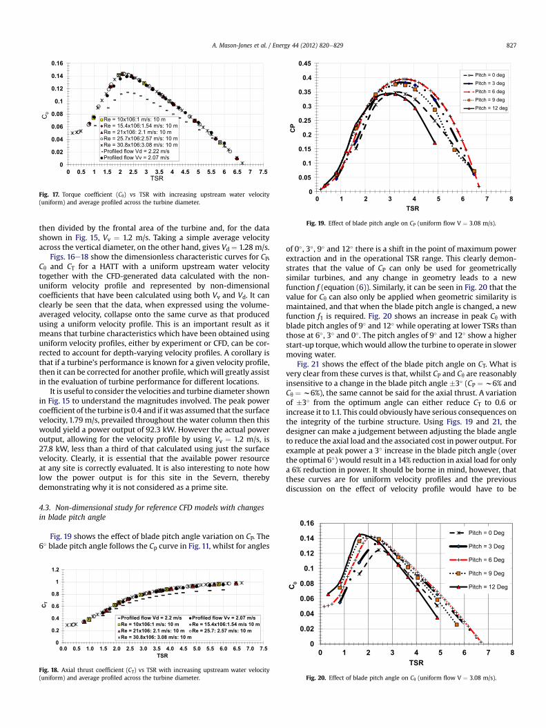
Fig. 19. Effect of blade pitch angle on CP (uniform flow V ¼ 3.08 m/s).

0.14

0.16

Pitch = 0 Deg

Pitch = 3 Deg

0

0.02

0.04

0.06

0.08

0.1

0.12

0.14

0.16

0 0.5 1 1.5 2 2.5 3 3.5 4 4.5 5 5.5 6 6.5 7 7.5

C

TSR

Re = 10x106:1 m/s: 10 mRe = 15.4x106:1.54 m/s: 10 mRe = 21x106: 2.1 m/s: 10 mRe = 25.7x106:2.57 m/s: 10 mRe = 30.8x106:3.08 m/s: 10 mProfiled flow Vd = 2.22 m/sProfiled flow Vv = 2.07 m/s

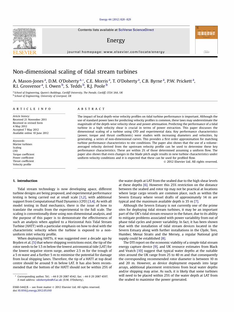
Fig. 17. Torque coefficient (Cq) vs TSR with increasing upstream water velocity(uniform) and average profiled across the turbine diameter.

A. Mason-Jones et al. / Energy 44 (2012) 820e829 827

then divided by the frontal area of the turbine and, for the datashown in Fig. 15, Vv ¼ 1.2 m/s. Taking a simple average velocityacross the vertical diameter, on the other hand, gives Vd ¼ 1.28 m/s.

Figs. 16e18 show the dimensionless characteristic curves for CP,Cq and CT for a HATT with a uniform upstream water velocitytogether with the CFD-generated data calculated with the non-uniform velocity profile and represented by non-dimensionalcoefficients that have been calculated using both Vv and Vd. It canclearly be seen that the data, when expressed using the volume-averaged velocity, collapse onto the same curve as that producedusing a uniform velocity profile. This is an important result as itmeans that turbine characteristics which have been obtained usinguniform velocity profiles, either by experiment or CFD, can be cor-rected to account for depth-varying velocity profiles. A corollary isthat if a turbine’s performance is known for a given velocity profile,then it can be corrected for another profile, which will greatly assistin the evaluation of turbine performance for different locations.

It is useful to consider the velocities and turbine diameter shownin Fig. 15 to understand the magnitudes involved. The peak powercoefficient of the turbine is 0.4 and if it was assumed that the surfacevelocity, 1.79 m/s, prevailed throughout the water column then thiswould yield a power output of 92.3 kW. However the actual poweroutput, allowing for the velocity profile by using Vv ¼ 1.2 m/s, is27.8 kW, less than a third of that calculated using just the surfacevelocity. Clearly, it is essential that the available power resourceat any site is correctly evaluated. It is also interesting to note howlow the power output is for this site in the Severn, therebydemonstrating why it is not considered as a prime site.

4.3. Non-dimensional study for reference CFD models with changesin blade pitch angle

Fig. 19 shows the effect of blade pitch angle variation on CP. The6� blade pitch angle follows the Cp curve in Fig. 11, whilst for angles

0

0.2

0.4

0.6

0.8

1

1.2

0.0 0.5 1.0 1.5 2.0 2.5 3.0 3.5 4.0 4.5 5.0 5.5 6.0 6.5 7.0 7.5

CT

TSR

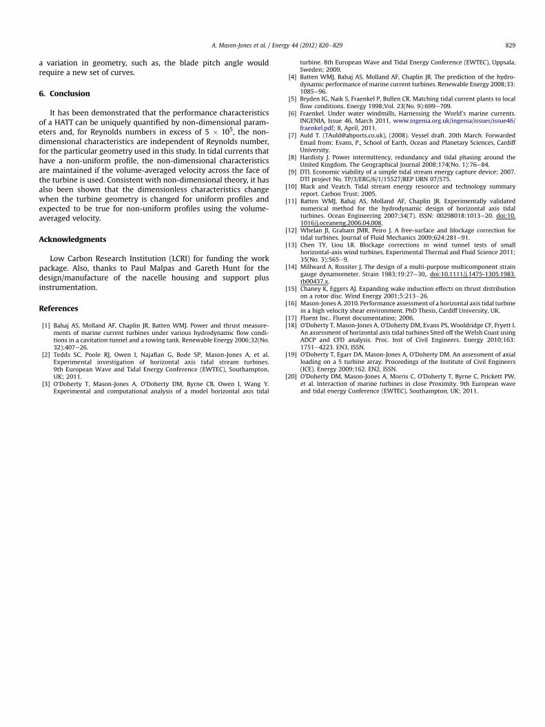
Profiled flow Vd = 2.2 m/s Profiled flow Vv = 2.07 m/s

Re = 10x106:1 m/s: 10 m Re = 15.4x106:1.54 m/s 10 m

Re = 21x106: 2.1 m/s: 10 m Re = 25.7: 2.57 m/s: 10 m

Re = 30.8x106: 3.08 m/s: 10 m

Fig. 18. Axial thrust coefficient (CT) vs TSR with increasing upstream water velocity(uniform) and average profiled across the turbine diameter.

of 0�, 3�, 9� and 12� there is a shift in the point of maximum powerextraction and in the operational TSR range. This clearly demon-strates that the value of CP can only be used for geometricallysimilar turbines, and any change in geometry leads to a newfunction f (equation (6)). Similarly, it can be seen in Fig. 20 that thevalue for Cq can also only be applied when geometric similarity ismaintained, and that when the blade pitch angle is changed, a newfunction f1 is required. Fig. 20 shows an increase in peak Cq withblade pitch angles of 9� and 12� while operating at lower TSRs thanthose at 6�, 3� and 0�. The pitch angles of 9� and 12� show a higherstart-up torque, which would allow the turbine to operate in slowermoving water.

Fig. 21 shows the effect of the blade pitch angle on CT. What isvery clear from these curves is that, whilst CP and Cq are reasonablyinsensitive to a change in the blade pitch angle �3� (CP ¼w6% andCq ¼ w6%), the same cannot be said for the axial thrust. A variationof �3� from the optimum angle can either reduce CT to 0.6 orincrease it to 1.1. This could obviously have serious consequences onthe integrity of the turbine structure. Using Figs. 19 and 21, thedesigner can make a judgement between adjusting the blade angleto reduce the axial load and the associated cost in power output. Forexample at peak power a 3� increase in the blade pitch angle (overthe optimal 6�) would result in a 14% reduction in axial load for onlya 6% reduction in power. It should be borne in mind, however, thatthese curves are for uniform velocity profiles and the previousdiscussion on the effect of velocity profile would have to be

0

0.02

0.04

0.06

0.08

0.1

0.12

0 1 2 3 4 5 6 7 8

C

TSR

Pitch = 6 Deg

Pitch = 9 Deg

Pitch = 12 Deg

Fig. 20. Effect of blade pitch angle on Cq (uniform flow V ¼ 3.08 m/s).

0

0.2

0.4

0.6

0.8

1

1.2

1.4

1.6

0 1 2 3 4 5 6 7 8

CT

TSR

Pitch = 0 Deg

Pitch = 3 Deg

Pitch = 6 Deg

Pitch = 9 Deg

Pitch = 12 Deg

Fig. 21. Effect of blade pitch angle on CT (uniform flow V ¼ 3.08 m/s).

A. Mason-Jones et al. / Energy 44 (2012) 820e829828

considered. In the case of a velocity profile, the turbine’s perfor-mance coefficients will fall within 2% of those predicted froma uniform velocity profile if the volumetric flow rate over theturbine’s swept area is used. Hence, changes in the characteristicswould also be expected for the non-uniform velocity profiles.However, since the terms are a function of V2 (torque and axialload) and V3 (power) then the coefficients are very sensitive to theaccuracy of the calculated velocity.

If the models for the different pitch angles are runwith Vv as theaverage velocity across the swept area, the results overlay thoseshown in Figs. 19e21.

5. Performance charts for prototype HATT design

In Section 4 it has been demonstrated that a particular design ofHATT can be uniquely characterised by dimensionless parameters,which can be quantified by experiment or CFD, provided the Rey-nolds number (based on turbine diameter) is greater than 5 � 105.The dimensionless characteristics can be applied to geometricallysimilar turbines, of different size, deployed in tidal currents withuniform or non-uniform velocity profiles, provided the volume-averaged velocity is used.

0

0.5

1

1.5

2

2.5

3

3.5

4

4.5

5

0 0.5 1 1.5Angular V

Po

we

r (M

W)

30 m

20 m

15 m

3.086 m/s

1.54 m/s

2.05 m/s

2.57 m/s

Fig. 22. Design specific peak power curves with increasing diameter a

Given the location discussed earlier for the HATT within theSevern Estuary and the restrictions imposed at the site due to localshipping lines, both the diameter and operational depth of theHATT are to some extent fixed. This type of restriction may well bea common problem at other sites especially if and when the tech-nology is expanded. Bearing in mind that the appropriate charac-teristic velocity for the turbine is the volume-averaged value,a minimum value of 1.54 m/s was chosen as the minimum inletvelocity, which is just above the recommended minimum cut-inflow velocity of 1 m/s [10]. Fig. 22 has been constructed for theturbine configuration used in this study and for the given velocityrange, using the optimum values of Cp and TSR of 0.4 and 3.6respectively from Fig. 11, and using volume-averaged inlet veloci-ties between 1.54 m/s and 3.086 m/s (3e6 knots) for a turbinediameter range between 6 m and 30 m. Using Fig. 22, it can beshown that to produce a rated power of 1 MW with the existingHATT design and a single rotor, a diameter of 15 m would berequired for a velocity of 3.08 m/s. At a mean spring peak velocity of2.57 m/s, typically discussed in literature, a diameter of approxi-mately 18 m would be required. Again, it should be rememberedthat it is volume-averaged velocities that are being discussed.

The introduction of a velocity profile through the water columnhas a significant effect on power attenuation through the waterdepth. The cube proportionality on the velocity component willsignificantly affect power extraction estimates when using nearsurface measurements. Large velocity and shear rates towards theseabed therefore have the potential to compromise the operation ofthe turbine. As in the case of the Severn Estuary it is more thanlikely that the rotational axis depth of the turbine will be greatlyinfluenced by local shipping restrictions. Using the scaling curves ofFig. 22 two rotors would be required with diameters of between15m and 20m tomeet the 1MW target typically quoted. For a largepart of the Severn Estuary it is more likely, due to large hull depth,that a turbine diameter would be restricted to around 10 m or less.Under these circumstances groups of between 4 and 6 turbineswould be necessary. Under these circumstances, and using thefindings of O’Doherty et al. [19,20], the spatial requirements forgroups or arrays of turbines can clearly be predetermined.

The principle of this work has shown that only a single set ofcharacteristic curves are needed in order to characterise theperformance of a specified turbine blade design. However,

2 2.5 3 3.5 4elocity w (rad/s)

10 m

6 m

nd tidal velocity with a maximum tidal velocity of 3.08 m/s [16].

A. Mason-Jones et al. / Energy 44 (2012) 820e829 829

a variation in geometry, such as, the blade pitch angle wouldrequire a new set of curves.

6. Conclusion

It has been demonstrated that the performance characteristicsof a HATT can be uniquely quantified by non-dimensional param-eters and, for Reynolds numbers in excess of 5 � 105, the non-dimensional characteristics are independent of Reynolds number,for the particular geometry used in this study. In tidal currents thathave a non-uniform profile, the non-dimensional characteristicsare maintained if the volume-averaged velocity across the face ofthe turbine is used. Consistent with non-dimensional theory, it hasalso been shown that the dimensionless characteristics changewhen the turbine geometry is changed for uniform profiles andexpected to be true for non-uniform profiles using the volume-averaged velocity.

Acknowledgments

Low Carbon Research Institution (LCRI) for funding the workpackage. Also, thanks to Paul Malpas and Gareth Hunt for thedesign/manufacture of the nacelle housing and support plusinstrumentation.

References

[1] Bahaj AS, Molland AF, Chaplin JR, Batten WMJ. Power and thrust measure-ments of marine current turbines under various hydrodynamic flow condi-tions in a cavitation tunnel and a towing tank. Renewable Energy 2006;32(No.32):407e26.

[2] Tedds SC, Poole RJ, Owen I, Najafian G, Bode SP, Mason-Jones A, et al.Experimental investigation of horizontal axis tidal stream turbines.9th European Wave and Tidal Energy Conference (EWTEC), Southampton,UK; 2011.

[3] O’Doherty T, Mason-Jones A, O’Doherty DM, Byrne CB, Owen I, Wang Y.Experimental and computational analysis of a model horizontal axis tidal

turbine. 8th European Wave and Tidal Energy Conference (EWTEC), Uppsala,Sweden; 2009.

[4] Batten WMJ, Bahaj AS, Molland AF, Chaplin JR. The prediction of the hydro-dynamic performance of marine current turbines. Renewable Energy 2008;33:1085e96.

[5] Bryden IG, Naik S, Fraenkel P, Bullen CR. Matching tidal current plants to localflow conditions. Energy 1998;Vol. 23(No. 9):699e709.

[6] Fraenkel. Under water windmills, Harnessing the World’s marine currents.INGENIA, Issue 46, March 2011, www.ingenia.org.uk/ingenia/issues/issue46/fraenkel.pdf; 8, April, 2011.

[7] Auld T. (TAuld@abports.co.uk), (2008). Vessel draft. 20th March. ForwardedEmail from: Evans, P., School of Earth, Ocean and Planetary Sciences, CardiffUniversity.

[8] Hardisty J. Power intermittency, redundancy and tidal phasing around theUnited Kingdom. The Geographical Journal 2008;174(No. 1):76e84.

[9] DTI. Economic viability of a simple tidal stream energy capture device; 2007.DTI project No. TP/3/ERG/6/1/15527/REP URN 07/575.

[10] Black and Veatch. Tidal stream energy resource and technology summaryreport. Carbon Trust; 2005.

[11] Batten WMJ, Bahaj AS, Molland AF, Chaplin JR. Experimentally validatednumerical method for the hydrodynamic design of horizontal axis tidalturbines. Ocean Engineering 2007;34(7). ISSN: 00298018:1013e20. doi:10.1016/j.oceaneng.2006.04.008.

[12] Whelan JI, Graham JMR, Peiro J. A free-surface and blockage correction fortidal turbines. Journal of Fluid Mechanics 2009;624:281e91.

[13] Chen TY, Liou LR. Blockage corrections in wind tunnel tests of smallhorizontal-axis wind turbines. Experimental Thermal and Fluid Science 2011;35(No. 3):565e9.

[14] Millward A, Rossiter J. The design of a multi-purpose multicomponent straingauge dynamometer. Strain 1983;19:27e30,. doi:10.1111/j.1475-1305.1983.tb00437.x.

[15] Chaney K, Eggers AJ. Expanding wake induction effects on thrust distributionon a rotor disc. Wind Energy 2001;5:213e26.

[16] Mason-Jones A. 2010. Performance assessment of a horizontal axis tidal turbinein a high velocity shear environment. PhD Thesis, Cardiff University, UK.

[17] Fluent Inc.. Fluent documentation; 2006.[18] O’Doherty T, Mason-Jones A, O’Doherty DM, Evans PS, Wooldridge CF, Fryett I.

An assessment of horizontal axis tidal turbines Sited off the Welsh Coast usingADCP and CFD analysis. Proc. Inst of Civil Engineers. Energy 2010;163:1751e4223. EN3, ISSN.

[19] O’Doherty T, Egarr DA, Mason-Jones A, O’Doherty DM. An assessment of axialloading on a 5 turbine array. Proceedings of the Institute of Civil Engineers(ICE). Energy 2009;162. EN2, ISSN.

[20] O’Doherty DM, Mason-Jones A, Morris C, O’Doherty T, Byrne C, Prickett PW,et al. Interaction of marine turbines in close Proximity. 9th European waveand tidal energy Conference (EWTEC), Southampton, UK; 2011.