non-linear vibrations of free-edge thin spherical shells: modal interaction rules … · ·...
TRANSCRIPT
International Journal of Solids and Structures 42 (2005) 3339–3373
www.elsevier.com/locate/ijsolstr
Non-linear vibrations of free-edge thin spherical shells:modal interaction rules and 1:1:2 internal resonance q
Oliver Thomas a,*, C. Touze b, A. Chaigne b
a Structural Mechanics and Coupled Systems Laboratory, CNAM, 2 rue Conte, 75003 Paris, Franceb ENSTA-UME, Chemin de la Huniere, 91761 Palaiseau Cedex, France
Received 23 June 2004; received in revised form 25 October 2004Available online 15 December 2004
Abstract
This paper is devoted to the derivation and the analysis of vibrations of shallow spherical shell subjected to largeamplitude transverse displacement. The analog for thin shallow shells of von Karman�s theory for large deflection ofplates is used. The validity range of the approximations is assessed by comparing the analytical modal analysis witha numerical solution. The specific case of a free edge is considered. The governing partial differential equations areexpanded onto the natural modes of vibration of the shell. The problem is replaced by an infinite set of coupled sec-ond-order differential equations with quadratic and cubic non-linear terms. Analytical expressions of the non-linearcoefficients are derived and a number of them are found to vanish, as a consequence of the symmetry of revolutionof the structure. Then, for all the possible internal resonances, a number of rules are deduced, thus predicting the acti-vation of the energy exchanges between the involved modes. Finally, a specific mode coupling due to a 1:1:2 internalresonance between two companion modes and an axisymmetric mode is studied.� 2004 Elsevier Ltd. All rights reserved.
Keywords: Shallow spherical shells; Geometrical non-linearities; Internal resonances, Non-linear vibrations
1. Introduction
Structures with a thin geometry, like beams, arches, plates and shells, can exhibit large amplitude flexuralvibrations, whose magnitude is comparable to the order of their thickness. In those cases, typical non-linear
0020-7683/$ - see front matter � 2004 Elsevier Ltd. All rights reserved.doi:10.1016/j.ijsolstr.2004.10.028
q This work was performed during a post-doctoral stay of the first author at ENSTA-UME.* Corresponding author. Tel.: +33 0158 80 85 80; fax: +33 0140 27 27 16.E-mail address: [email protected] (O. Thomas).

3340 O. Thomas et al. / International Journal of Solids and Structures 42 (2005) 3339–3373
behaviors can be observed, such as jump phenomena and energy exchanges between modal configurationsand a linear prediction model is not sufficient (Nayfeh and Mook, 1979). In this paper, von Karmannon-linear dynamic equations are used in the special case of a shallow spherical cap in order to predictand simulate the observed phenomena.
In the literature devoted to geometrically non-linear (finite-amplitude) vibrations of shells, the largestpart of the studies is concerned with circular cylindrical shells. The interested reader can refer to theexhaustive review proposed by (Amabili et al., 1998). For the case of spherical caps, most of the studiesincluding geometrical non-linearities deal with axisymmetric deflections of perfectly symmetric structures.Moreover, the focus is generally put on dynamic buckling and snap-through behavior, whereas vibratoryresponses are seldom treated. Some works dealing with non-linear vibration of shells are briefly reviewedhere and the interested reader can refer for a thorough bibliography to reviews of the literature by Leissa(1993b), Qatu (2002), Moussaoui and Benamar (2002) as well as the recent paper by Amabili andPaıdoussis (2003). Evensen and Evan-Iwanowsky (1967) proposed a very complete work, analyticaland experimental, and investigate buckling as well as non-linear vibrations of a clamped-edge sphericalcap with the harmonic balance method. Goncalves (1994) addressed the same problem, with geometricalimperfections, and used a Galerkin method with the analytical expressions of the mode shapes to solve theproblem. Ye (1997) used a numerical Runge–Kutta method to solve the same problem. However, thosestudies are restricted to vibrations involving only one axisymmetric mode. A detailed study is proposed byYasuda and Kushida (1984) who investigated the multi-mode axisymmetric response of a clamped spher-ical cap. The special case of a 1:2 internal resonance between two axisymmetric modes was addressed boththeoretically and experimentally. Grossman et al. (1969) investigated the free oscillations axisymmetricfrequencies dependence with the deflection amplitude, as a function of both the curvature of the shelland the boundary conditions. All those studies are restricted to axisymmetric vibrations. However, evenif the excitation pattern is rotationally symmetric, a complete realistic study has to include asymmetricvibrations, since non-linear coupling between any modal configuration is likely to appear. Hui (1983) ad-dressed one-mode asymmetric vibrations of a complete spherical shell with geometric imperfections andstructural damping. To the knowledge of the authors, no analytical studies on non-linear multi-modeasymmetric vibrations of spherical shells have been published and the present work aims at filling thisgap.
Spherical caps can be considered as a reference problem, mainly because their vibrations display impor-tant non-linear behaviors that are commonly observed in large deflection vibrations of thin structures.Firstly, as a consequence of the multiplicity of two of eigenfrequencies associated to asymmetricmodes—a common feature of structures with an axisymmetric geometry (see e.g. Morand and Ohayon,1995, Chapter 1)—1:1 internal resonances between companion modes are numerous and give rise to a vari-ety of complex vibratory patterns, including traveling waves (see e.g. Tobias and Arnold, 1957; Raman andMote, 2001; Touze et al., 2002). Secondly, the curvature of the structure adds quadratic non-linearities inthe oscillators that govern the dynamics of the system, whereas only cubic terms are present in the case oftransversely symmetric structures such as rods and plates (Thomas et al., 2001). Thirdly, the spectral con-tent of spherical shells depends on one geometrical parameter related to the curvature. Particular algebraicrelations between natural frequencies can then be obtained for specific values of the curvature. As a con-sequence, numerous internal resonances that are related to both quadratic and cubic non-linear terms arelikely to be observed on spherical shells. An example addressed in the present work is the 1:1:2 internal res-onance between an axisymmetric mode and two companion modes.
The main goal of this paper is to present a exhaustive method for analysis and prediction of the largeamplitude vibratory response of spherical shells, from the governing equations to their resolution. It ex-tends a study on non-linear vibrations of circular plates (Touze et al., 2002) to the case a curved shallowgeometry. The non-linear behavior and the possible energy transfers between modal configurations relatedto the perfect axisymmetric geometry of the structure are especially addressed, extending results of the
O. Thomas et al. / International Journal of Solids and Structures 42 (2005) 3339–3373 3341
literature. The free-edge boundary conditions have been chosen mainly because they are the easiest torealize experimentally. However, the results of the present study can be extended to any type of boundaryconditions, provided they are in accordance with the rotational symmetry of the problem.
The non-linear partial differential equations (PDE) that govern the oscillations of the shell are ex-panded onto its eigenmodes. The main underlying assumptions of the model, as well as the hypothesisof shallowness, are discussed. Complete analytical expressions of the eigenmodes of the associated linearproblem are derived and compared to a numerical solution. After expansion of the PDE onto the eigen-modes, a set of coupled second-order ordinary differential equations with quadratic and cubic non-linearities is obtained. The coefficients of the non-linear terms are calculated in the case of a perfectaxisymmetric geometry and the coupling rules for the modal interactions are deduced. Possible truncationof the infinite dimensional problem are evaluated. Finally, the particular case of a 1:1:2 internal resonanceis precisely investigated by a perturbation method, in the case of a harmonic forced excitation. The effectof slight imperfections of the structure is simulated by introducing slight differences in the companionmodes frequencies. Experimental validations of the theoretical results will be presented in a forthcomingpaper.
2. Formulation of the problem
2.1. Local equations
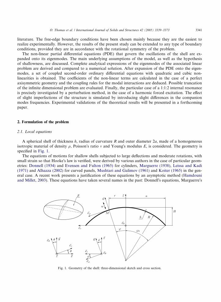
A spherical shell of thickness h, radius of curvature R and outer diameter 2a, made of a homogeneousisotropic material of density q, Poisson�s ratio m and Young�s modulus E, is considered. The geometry isspecified in Fig. 1.
The equations of motions for shallow shells subjected to large deflections and moderate rotations, withsmall strain so that Hooke�s law is verified, were derived by various authors in the case of particular geom-etries: Donnell (1934) and Evensen and Fulton (1965) for cylinders, Marguerre (1938), Leissa and Kadi(1971) and Alhazza (2002) for curved panels, Mushtari and Galimov (1961) and Koiter (1965) in the gen-eral case. A recent work presents a justification of these equations by an asymptotic method (Hamdouniand Millet, 2003). These equations have taken several names in the past: Donnell�s equations, Marguerre�s
Fig. 1. Geometry of the shell: three-dimensional sketch and cross section.
3342 O. Thomas et al. / International Journal of Solids and Structures 42 (2005) 3339–3373
equations, Koiter�s equations or von Karman�s equations. They correspond to a generalization to the caseof a curved geometry of von Karman�s model for large-deflection vibrations of plates (see e.g. Chu andHerrmann, 1956).
The main hypotheses are the following (see e.g. Koiter, 1965; Soedel, 1981):
• the shell is thin: h/a� 1 and h/R� 1;• the shell is shallow: a/R� 1;• the transverse normal stress are neglected with respect to the other stresses;• Kirchhoff–Love hypotheses are used: the shear-strains are neglected and the normals to the undeformed
mid-surface remain straight and normal and suffer no extension during the deformation;• rotations of normals to the mid-surface are moderate, so that their sine and cosine are linearized (mod-
erate rotations hypothesis);• only the non-linear terms of the lowest order are kept in the strain expressions;• the material is linear elastic, homogeneous and isotropic;• in-plane and rotatory inertia are neglected;• there is no membrane external forcing, which enables the use of an Airy stress function F.
With these assumptions fulfilled, one obtains the equations of motion in terms of the transverse displace-ment w along the normal to the mid-surface and the Airy stress function F, for all time t
DDDw þ 1
RDF þ qh€w ¼ Lðw; F Þ � c _w þ p; ð1aÞ
DDF � EhR
Dw ¼ �Eh2
Lðw;wÞ; ð1bÞ
where D = Eh3/12(1 � m2) is the flexural rigidity, c is a damping coefficient, p represents the external normalpressure, €w is the second partial derivative of w with respect to time, D is the Laplacian and L is a bilinearquadratic operator. With the assumption that the shell is shallow, angle u defined in Fig. 1 is small and weget
sin u ’ u; r ¼ R sin u ’ Ru: ð2Þ
Hence, the position of any point of the middle surface of the shell can be measured by its polar coordinates(r,h), r 2 [0;a] and h 2 [0;2p] and the operators D and L of Eqs. (1a) and (1b) can be written
DðÞ ¼ ðÞ;rr þ1
rðÞ;r þ
1
r2ðÞ;hh ð3Þ
and
Lðw; F Þ ¼ w;rrF ;r
rþ F ;hh
r2
� �þ F ;rr
w;r
rþ w;hh
r2
� �� 2
w;rh
r� w;h
r2
� � F ;rh
r� F ;h
r2
� �; ð4Þ
where (Æ),ab = o2(Æ)/oaob. Expressions of F as a function of membrane stresses can be found in Touze et al.(2002). Quadratic operator L defined by Eq. (4) has the same expression as in von Karman�s equations forcircular plates (Efstathiades, 1971). A proof of Eqs. (1a) and (1b) can be obtained after writing the doublycurved panel equations formulated in Leissa and Kadi (1971) in polar coordinates.
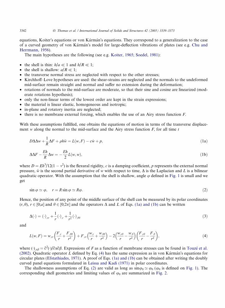
The shallowness assumptions of Eq. (2) are valid as long as sinu0 ’ u0 (u0 is defined on Fig. 1). Thecorresponding shell geometries and limiting values of u0 are summarized in Fig. 2.
Fig. 2. Shell geometry so that Eqs. (2) are fulfilled, with sinu0=a/R. Parameters are defined on Fig. 1.
O. Thomas et al. / International Journal of Solids and Structures 42 (2005) 3339–3373 3343
2.2. Free-edge boundary conditions
Boundary conditions are similar to those of a free-edge circular plate (Touze et al., 2002) which yields forall t and h
F and w are bounded at r ¼ 0; ð5aÞ
F ;r þ1
aF ;hh ¼ 0; F ;rh �
1
aF ;h ¼ 0; at r ¼ a; ð5bÞ
w;rr þmaw;r þ
ma2
w;hh ¼ 0; at r ¼ a; ð5cÞ
w;rrr þ1
aw;rr �
1
a2w;r þ
2 � ma2
w;rhh �3 � ma3
w;hh ¼ 0; at r ¼ a: ð5dÞ
The above equations stems from the vanishing of the external load at the edge: Eqs. (5b) are related to themembrane forces, Eq. (5c) to the bending moment and Eq. (5d) to the twisting moment and transverseshear force.
2.3. Dimensional analysis
Equations of motion (1a) and (1b) group different terms. On the one hand, terms DF in Eq. (1a) and Dwin Eq. (1b) are responsible for a linear coupling between transverse motion and membrane stretching, stem-ming from the curved geometry of the shell. On the other hand, terms L(Æ, Æ) in both equations produce anon-linear coupling. Those two effects are independent from each other, since operator L is independent ofcurvature R. If R tends to infinity, one obtains von Karman�s equations (Efstathiades, 1971) for geometri-cally non-linear plates and if L(Æ, Æ) vanishes, linear Donnell–Mushtari–Vlasov�s model (Soedel, 1981) forshallow shells is obtained.
As the longitudinal inertia is neglected, F is slaved to transverse displacement w. Eq. (1b) shows that Fcontains both a linear and a quadratic term in w. By substituting F in Eq. (1a), one can show that curvatureand non-linear coupling create together a linear, a quadratic and a cubic term in the equation that governsw, the first two terms arising from curvature. In order to balance their magnitude, dimensionless quantities(denoted by overbars) are introduced
w ¼ w0�w; F ¼ F 0�F ; r ¼ a�r; t ¼ T 0�t; with T 0 ¼ a2
ffiffiffiffiffiffiqhD
r: ð6Þ
w0 and F0 will be specified next. Substituting these variables in Eqs. (1a) and (1b) and omitting for claritydamping and forcing terms, one obtains for Eq. (1a)
TableAnaly(a/R =
a/R
000.010.010.10.1
v, eq a
3344 O. Thomas et al. / International Journal of Solids and Structures 42 (2005) 3339–3373
DDw þ €w ¼ �vf�wg þ 1
2eqf�w2g � ecf�w3g; ð7Þ
where f�wng denotes a dimensionless term proportional to �wn supposed to be O(1). The order of magnitudeof the different terms in Eq. (7) are specified by the following dimensionless factors:
linear term f�wg : v ¼ Eha4
DR2¼ 12ð1 � m2Þ a4
R2h2; ð8aÞ
quadratic term f�w2g : eq ¼ Eha2
DRw0 ¼ 12ð1 � m2Þ a2
Rh2w0; ð8bÞ
cubic term f�w3g : ec ¼EhD
w20 ¼ 12ð1 � m2Þw
20
h2: ð8cÞ
From these developments it appears naturally that curvature adds a linear term, which depends on thegeometry of the shell only (parameter v): it corresponds to the increase of transverse rigidity of the structurebrought by the linear coupling between transverse motion and mid-plane stretching. It will be shown that vbrings a correction to the shell eigenfrequencies compared to those of the corresponding plate (Section 3.1).
Non-linear terms have the order of magnitude of eq and ec, which depends on the scaling w0 of transversedisplacement. As
ec ¼ e2q=v; ð9Þ
we find that cubic terms are of one order of magnitude smaller than that of quadratic terms. It is the usualscaling chosen for those terms when a perturbation method is used to solve the problem, so that these termsappear successively in the perturbative scheme (Nayfeh and Mook, 1979). We can also remark that thecoefficient of cubic terms ec is independent of curvature R and that it is equal to the value it has in the caseof a plate.
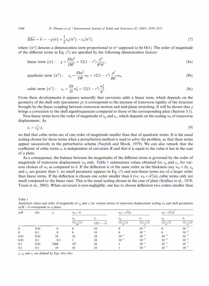
As a consequence, the balance between the magnitudes of the different terms is governed by the order ofmagnitude of transverse displacement w0 only. Table 1 summarizes values obtained for eq and ec, for var-ious choices of w0 as compared to h. If the deflection is of the same order as the thickness (say w0 = h), eqand ec are greater than 1, no small parameter appears in Eq. (7) and non-linear terms are of a larger orderthan linear terms. If the deflection is chosen one order smaller than h (i.e. w0 = h2/a), cubic terms only aresmall compared to the linear ones. This is the usual scaling chosen in the case of plate (Sridhar et al., 1978;Touze et al., 2002). When curvature is non-negligible, one has to choose deflection two orders smaller than
1tical values and order of magnitude of eq and ec for various choice of transverse displacement scaling w0 and shell geometries0 corresponds to a plate)
h/a v w0 = h w0 = h2/a w0 = h3/a2
eq ec eq ec eq ec12ð1�m2Þa2
Rh 12(1 � m2) 12ð1�m2ÞaR
12ð1�m2Þh2
a2
12ð1�m2ÞhR
12ð1�m2Þh4
a4
0.01 0 0 10 0 10�3 0 10�7
0.1 0 0 10 0 10�1 0 10�3
0.01 10 10 10 10�1 10�3 10�3 10�7
0.1 0.1 1 10 10�1 10�1 10�2 10�3
0.01 1000 102 10 1 10�3 10�2 10�7
0.1 10 10 10 1 10�1 10�1 10�3
nd ec are defined by Eqs. (8a)–(8c).
O. Thomas et al. / International Journal of Solids and Structures 42 (2005) 3339–3373 3345
thickness (w0 = h3/a2) to obtain both quadratic and cubic terms smaller than the linear ones. This is thesolution adopted here since a perturbation method will be used in Section 5 to solve Eqs. (1a) and (1b).The above developments about scaling of the deflection w0 show that non-linear phenomena become sig-nificant in curved structures for deflections of an order of magnitude between h3/a2 and h2/a, smaller thanin the case of plates.
The scaling F0 of the stress function is chosen so that dimensionless variable F is O(1) whenDDF ’ �1=2Lðw;wÞ in Eq. (1b). This solution is suitable for any R, especially if R tends to infinity (the caseof a plate). The following dimensionless variables are then defined:
r ¼ a�r; t ¼ a2ffiffiffiffiffiffiffiffiffiffiffiqh=D
p�t; w ¼ h3=a2�w; F ¼ Eh7=a4�F ; ð10aÞ
c ¼ ½2Eh4=Ra2 ffiffiffiffiffiffiffiffiffiffiffiqh=D
p�l; p ¼ Eh7=Ra6�p: ð10bÞ
Substituting the above definitions in equations of motion (1a) and (1b) and dropping the overbars in theresults, one obtains
DDw þ eqDF þ €w ¼ ecLðw; F Þ þ eq½�2l _w þ p ; ð11aÞ
DDF � a4
Rh3Dw ¼ � 1
2Lðw;wÞ; ð11bÞ
where eq = 12(1 � m2)h/R and ec = 12(1 � m2)h4/a4. Boundary conditions (5a)–(5d), take the same form,with a = 1. Forcing and damping terms are scaled to the order of quadratic terms since only those nonlinearterms will be retained in the study of Section 5.
3. Modal analysis of the linear problem
3.1. Eigenfrequencies and mode shapes
An analytical expression of the natural frequencies of vibration of spherical shells with free-edge, axi-symmetric as well as asymmetric, was proposed by Johnson and Reissner (1956). The main steps of the der-ivation of the expressions of the natural frequencies and mode shapes can be found in Appendix A and onlysome remarks are considered here.
The eigenmodes of the problem are the solutions of
DDU þ vDW � x2U ¼ 0; ð12aÞ
DDW ¼ DU: ð12bÞ
They depend on one geometrical parameter only, the curvature parameter v, that includes the joint influ-ence of R, a and h. Transverse and membrane mode shapes Ukn(r,h) and Wkn(r,h) have k nodal diametersand n nodal circles. Associated dimensionless angular frequencies xkn are related to their dimensionedcounterpart fkn (in Hz) by the formulafkn ¼1
2pa2
ffiffiffiffiffiffiDqh
sxkn ¼
h2pa2
ffiffiffiffiffiffiffiffiffiffiffiffiffiffiffiffiffiffiffiffiffiffiffiffiE
12qð1 � m2Þ
sxkn: ð13Þ
As membrane inertia is neglected, membrane motion is slaved to transverse motion. There are no mem-brane natural frequencies and each eigenfrequency xkn is associated to Ukn(r,h) and Wkn(r,h) (Kalnins,1964).
3346 O. Thomas et al. / International Journal of Solids and Structures 42 (2005) 3339–3373
The modes with at least one nodal diameter (k P 1) are called asymmetric modes. Each associated eigen-frequency has a multiplicity of two and the two corresponding independent modes are called companion orpreferential configurations. The deformed shape of the first deduces from the other by a rotation of p/2karound the symmetry axis.
3.2. Dependence on curvature
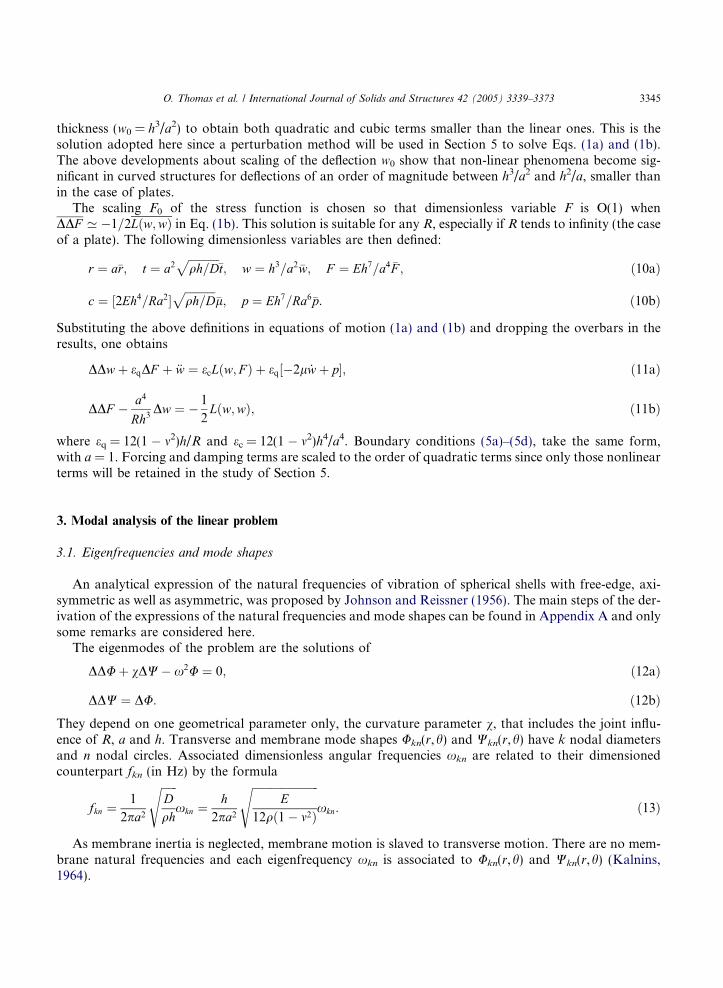
Fig. 3 shows the evolutions of several eigenfrequencies xkn with curvature parameter v and suggests toclassify the modes in two families.
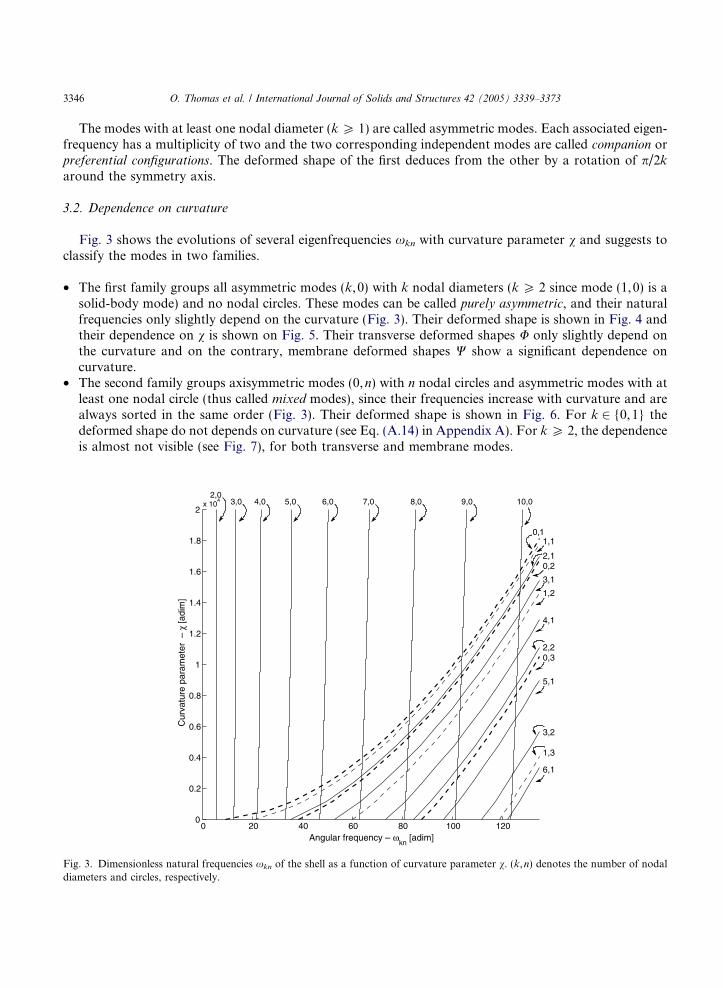
• The first family groups all asymmetric modes (k, 0) with k nodal diameters (k P 2 since mode (1,0) is asolid-body mode) and no nodal circles. These modes can be called purely asymmetric, and their naturalfrequencies only slightly depend on the curvature (Fig. 3). Their deformed shape is shown in Fig. 4 andtheir dependence on v is shown on Fig. 5. Their transverse deformed shapes U only slightly depend onthe curvature and on the contrary, membrane deformed shapes W show a significant dependence oncurvature.
• The second family groups axisymmetric modes (0,n) with n nodal circles and asymmetric modes with atleast one nodal circle (thus called mixed modes), since their frequencies increase with curvature and arealways sorted in the same order (Fig. 3). Their deformed shape is shown in Fig. 6. For k 2 {0,1} thedeformed shape do not depends on curvature (see Eq. (A.14) in Appendix A). For k P 2, the dependenceis almost not visible (see Fig. 7), for both transverse and membrane modes.
0 20 40 60 80 100 1200
0.2
0.4
0.6
0.8
1
1.2
1.4
1.6
1.8
2x 10
4
Angular frequency – ωkn
[adim]
Cur
vatu
re p
aram
eter
– χ
[adi
m]
6,1
1,3
3,2
5,1
0,32,2
4,1
1,2
3,1
0,22,1
0,1
10,09,08,07,06,05,04,03,02,0
1,1
Fig. 3. Dimensionless natural frequencies xkn of the shell as a function of curvature parameter v. (k,n) denotes the number of nodaldiameters and circles, respectively.
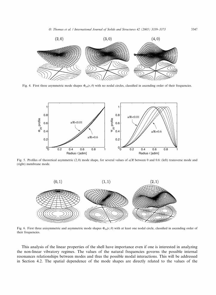
Fig. 4. First three asymmetric mode shapes Ukn(r,h) with no nodal circles, classified in ascending order of their frequencies.
0 0.2 0.4 0.6 0.8 10
0.2
0.4
0.6
0.8
1
Radius r [adim]
Φ20
pro
file
0 0.2 0.4 0.6 0.8 10
0.2
0.4
0.6
0.8
1
Radius r [adim]
Ψ20
pro
file a/R<0.01
a/R=0.6
a/R<0.01
a/R=0.6
Fig. 5. Profiles of theoretical asymmetric (2,0) mode shape, for several values of a/R between 0 and 0.6: (left) transverse mode and(right) membrane mode.
Fig. 6. First three axisymmetric and asymmetric mode shapes Ukn(r,h) with at least one nodal circle, classified in ascending order oftheir frequencies.
O. Thomas et al. / International Journal of Solids and Structures 42 (2005) 3339–3373 3347
This analysis of the linear properties of the shell have importance even if one is interested in analyzingthe non-linear vibratory regimes. The values of the natural frequencies governs the possible internalresonances relationships between modes and thus the possible modal interactions. This will be addressedin Section 4.2. The spatial dependence of the mode shapes are directly related to the values of the
0 0.2 0.4 0.6 0.8 1
–1
–0.5
0
0.5
1Φ
kn p
rofil
e
Radius r [adim]0 0.2 0.4 0.6 0.8 1
0
0.5
1
Ψkn
pro
file
Radius r [adim]
(0,1)
(2,1)
(0,1)
(1,1)(1,1)
(2,1)
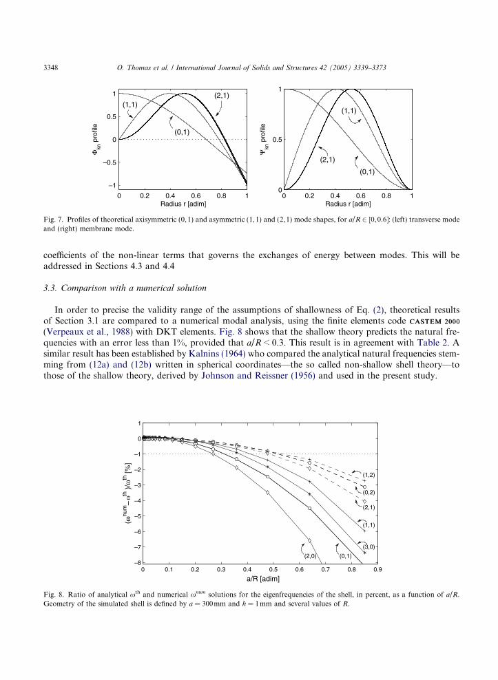
Fig. 7. Profiles of theoretical axisymmetric (0,1) and asymmetric (1,1) and (2,1) mode shapes, for a/R 2 [0,0.6]: (left) transverse modeand (right) membrane mode.
3348 O. Thomas et al. / International Journal of Solids and Structures 42 (2005) 3339–3373
coefficients of the non-linear terms that governs the exchanges of energy between modes. This will beaddressed in Sections 4.3 and 4.4
3.3. Comparison with a numerical solution
In order to precise the validity range of the assumptions of shallowness of Eq. (2), theoretical resultsof Section 3.1 are compared to a numerical modal analysis, using the finite elements code CASTEM 2000CASTEM 2000
(Verpeaux et al., 1988) with DKT elements. Fig. 8 shows that the shallow theory predicts the natural fre-quencies with an error less than 1%, provided that a/R < 0.3. This result is in agreement with Table 2. Asimilar result has been established by Kalnins (1964) who compared the analytical natural frequencies stem-ming from (12a) and (12b) written in spherical coordinates—the so called non-shallow shell theory—tothose of the shallow theory, derived by Johnson and Reissner (1956) and used in the present study.
0 0.1 0.2 0.3 0.4 0.5 0.6 0.7 0.8 0.9–8
–7
–6
–5
–4
–3
–2
–1
0
1
(ωnu
mωth
)/ω
th [%
]
a/R [adim]
(3,0)
(1,1)
(2,1)
(0,2)
(1,2)
(0,1)(2,0)
–
Fig. 8. Ratio of analytical xth and numerical xnum solutions for the eigenfrequencies of the shell, in percent, as a function of a/R.Geometry of the simulated shell is defined by a = 300mm and h = 1mm and several values of R.
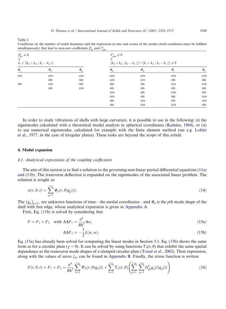
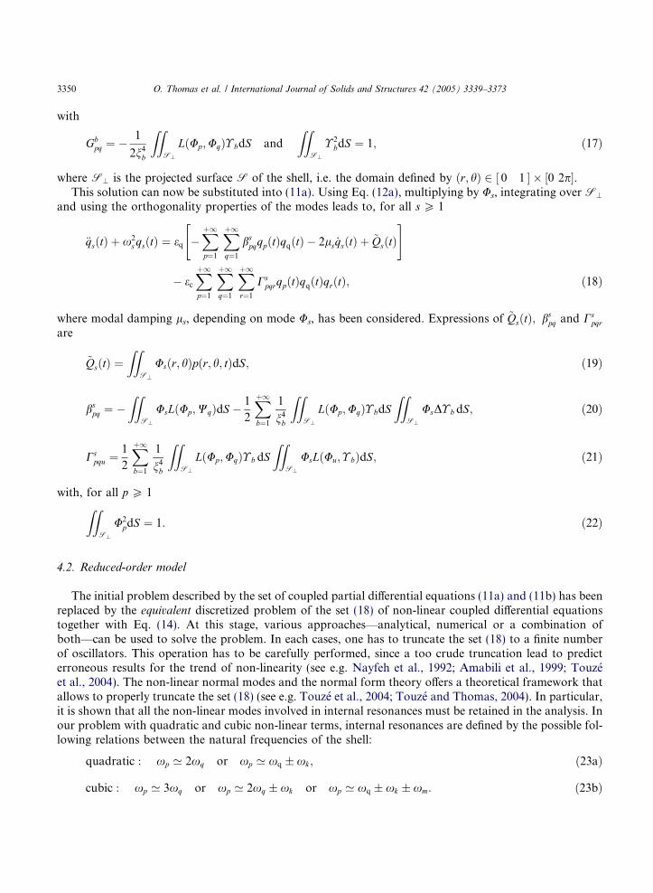
Table 2Conditions on the number of nodal diameters and the expression in sine and cosine of the modes (both conditions must be fulfilledsimultaneously) that lead to non-zero coefficients bs
pq and Cspqu
bspq 6¼ 0
+ks 2 fkp þ kq; j kp � kq jg
Cspqu 6¼ 0
+fkp þ kq; j kp � kq jg \ fks þ ku; j ks � ku jg 6¼ ;
Us Up Uq Up Uq Us Uu
cos cos cos cos cos cos cossin sin cos cos sin sin
sin cos sin sin sin cos cossin cos sin sin sin sin
cos sin cos sincos sin sin cossin cos sin cossin cos cos sin
O. Thomas et al. / International Journal of Solids and Structures 42 (2005) 3339–3373 3349
In order to study vibrations of shells with large curvature, it is possible to use in the following: (i) theeigenmodes calculated with a theoretical modal analysis in spherical coordinates (Kalnins, 1964), or (ii)to use numerical eigenmodes, calculated for example with the finite element method (see e.g. Lobitzet al., 1977, in the case of irregular plates). These tasks are beyond the scope of this article.
4. Modal expansion
4.1. Analytical expressions of the coupling coefficients
The aim of this section is to find a solution to the governing non-linear partial differential equations (11a)and (11b). The transverse deflection is expanded on the eigenmodes of the associated linear problem. Thesolution is sought as
wðr; h; tÞ ¼Xþ1
p¼1
Upðr; hÞqpðtÞ: ð14Þ
The fqpgp2N� are unknown functions of time—the modal coordinates—and Up is the pth mode shape of theshell with free edge, whose analytical expression is given in Appendix A.
First, Eq. (11b) is solved by considering that
F ¼ F 1 þ F 2 with DDF 1 ¼a4
Rh3Dw; ð15aÞ
DDF 2 ¼ � 1
2Lðw;wÞ: ð15bÞ
Eq. (15a) has already been solved for computing the linear modes in Section 3.1. Eq. (15b) shows the sameform as for a circular plate (v = 0). It can be solved by using functions � b(r,h) that exhibit the same spatialdependence as the transverse mode shapes of a clamped circular plate (Touze et al., 2002). Their expression,along with the values of zeros nb, can be found in Appendix B. Finally, the stress function is written
F ðr; h; tÞ ¼ F 1 þ F 2 ¼a4
Rh3
Xþ1
b¼1
Wbðr; hÞqbðtÞ þXþ1
b¼1
� bðr; hÞXþ1
p¼1
Xþ1
q¼1
GbpqqpðtÞqqðtÞ
!ð16Þ
3350 O. Thomas et al. / International Journal of Solids and Structures 42 (2005) 3339–3373
with
Gbpq ¼ � 1
2n4b
ZZS?
LðUp;UqÞ� bdS and
ZZS?
� 2bdS ¼ 1; ð17Þ
where S? is the projected surface S of the shell, i.e. the domain defined by ðr; hÞ 2 0 1½ � ½0 2p .This solution can now be substituted into (11a). Using Eq. (12a), multiplying by Us, integrating over S?
and using the orthogonality properties of the modes leads to, for all s P 1
€qsðtÞ þ x2s qsðtÞ ¼ eq �
Xþ1
p¼1
Xþ1
q¼1
bspqqpðtÞqqðtÞ � 2ls _qsðtÞ þ ~QsðtÞ
" #
� ec
Xþ1
p¼1
Xþ1
q¼1
Xþ1
r¼1
CspqrqpðtÞqqðtÞqrðtÞ; ð18Þ
where modal damping ls, depending on mode Us, has been considered. Expressions of ~QsðtÞ; bspq and Cs
pqr
are
~QsðtÞ ¼ZZ
S?
Usðr; hÞpðr; h; tÞdS; ð19Þ
bspq ¼ �
ZZS?
UsLðUp;WqÞdS � 1
2
Xþ1
b¼1
1
n4b
ZZS?
LðUp;UqÞ� bdSZZ
S?
UsD� b dS; ð20Þ
Cspqu ¼
1
2
Xþ1
b¼1
1
n4b
ZZS?
LðUp;UqÞ� b dSZZ
S?
UsLðUu; � bÞdS; ð21Þ
with, for all p P 1
ZZS?U2pdS ¼ 1: ð22Þ
4.2. Reduced-order model
The initial problem described by the set of coupled partial differential equations (11a) and (11b) has beenreplaced by the equivalent discretized problem of the set (18) of non-linear coupled differential equationstogether with Eq. (14). At this stage, various approaches—analytical, numerical or a combination ofboth—can be used to solve the problem. In each cases, one has to truncate the set (18) to a finite numberof oscillators. This operation has to be carefully performed, since a too crude truncation lead to predicterroneous results for the trend of non-linearity (see e.g. Nayfeh et al., 1992; Amabili et al., 1999; Touzeet al., 2004). The non-linear normal modes and the normal form theory offers a theoretical framework thatallows to properly truncate the set (18) (see e.g. Touze et al., 2004; Touze and Thomas, 2004). In particular,it is shown that all the non-linear modes involved in internal resonances must be retained in the analysis. Inour problem with quadratic and cubic non-linear terms, internal resonances are defined by the possible fol-lowing relations between the natural frequencies of the shell:
quadratic : xp ’ 2xq or xp ’ xq � xk; ð23aÞ
cubic : xp ’ 3xq or xp ’ 2xq � xk or xp ’ xq � xk � xm: ð23bÞ
O. Thomas et al. / International Journal of Solids and Structures 42 (2005) 3339–3373 3351
4.3. Coupling rules
For a perfect axisymmetric structure, mode shapes with k nodal diameter are written in terms of coskhand sinkh. As coefficients bs
pq and Cspqu involve integrations of products of those functions (see Eqs. (20) and
(21)), a number of them vanish. The goal of the present section is to exhibit some rules that determine whichcoefficients vanish and consequently which modal interactions are possible. The mathematical derivationscan be found in Appendix C.
Conditions for bspq and Cs
pqu to be non-zero are summarized in Table 2. They depend on (i) the number ofnodal diameters ks, kp, kq and ku of the modes Us, Up, Uq and Uu involved in the calculation of bs
pq and Cspqu
and (ii) the angular dependence in coskh or sinkh of each of Us, Up, Uq and Uu. The number n of nodalcircles has no influence.
Among those coefficients, some of them are involved in resonant non-linear terms. Those terms are calledresonant because they can be viewed as forcing terms that excite a particular mode close to its resonance,when internal resonances relations between the natural frequencies exist. They are thus responsible forstrong coupling—and thus large energy exchanges—between modal configurations. They cannot be re-moved by the computation of the normal form and thus govern the dynamics of the system (Guckenheimerand Holmes, 1983). As some coefficients vanish, the corresponding resonant terms are canceled and certainenergy exchanges are impossible, even if relations of the form of Eqs. (23a) and (23b) are fulfilled. The endof this section exhibits a few rules that enable to predict the possible modal interactions.
In order to determinate if a particular modal interaction is possible, one has (i) to check if any of Eqs.(23a) and (23b) is fulfilled and (ii) to check if the associated resonant terms are non zero, using the followingrules that hold on the number of nodal diameters of the involved modes. The rules holding on the nature insine or cosine of companion modes are secondary because they cannot be responsible of cancellation of allresonant terms in a particular internal resonance. They are thus not addressed here.
The first rule stands that all axisymmetric modes can be involved in modal interactions with one another, byboth order-two (Eq. (23a)) and order three (Eq. (23b)) internal resonances. Studies on modal interactions be-tween axisymmetric modes were proposed by Sridhar et al. (1975) for circular plates and by Yasuda andKushida (1984) in the case of spherical shells. The other rules, specifically related to particular internal res-onances involving asymmetric modes, are given below. One should keep in mind that two asymmetricmodes with natural frequencies such that x2 > x1 can have their numbers of nodal diameters such thatk2 < k1: this situation exists if the numbers of nodal circles are such that n2 > n1 (see e.g. Fig. 3).
4.3.1. Order-two internal resonances
The coupling rules are summarized in Tables 3 and 4. Each table specifies the internal resonance consid-ered (first line), the involved modes (second line), the resonant terms (third line) and the general conditions
Table 3Rules determining if modal interaction between modes U1 and U2 is possible, when internal resonance x2 = 2x1 is fulfilled
x2 = 2x1
Modes U1 (x1, k1) U2 (x2, k2)Resonant terms q1q2 q2
1
Rules k1 2 {k1 + k2,jk1 � k2j} 5 ; k2 2 {2k2,0} 5 ;Nature of involved modes Modal interaction
Both modes axisymmetric: k1 = k2 = 0 PossibleOnly mode U1 asymmetric: k1 5 0, k2 = 0 Possible "k1
Only mode U2 asymmetric: k1 = 0, k2 5 0 ImpossibleBoth modes asymmetric: k1 5 0, k2 5 0 Possible if k2 = 2k1
kp is the number of nodal diameters of mode Up, and qp is the time evolution of mode Up in set (18).
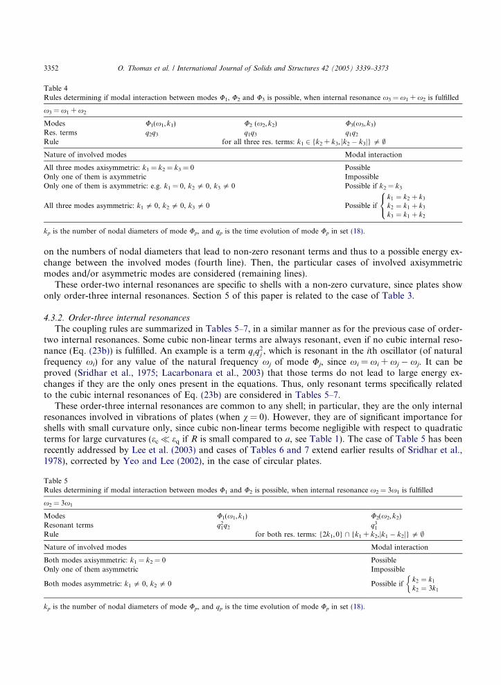
Table 4Rules determining if modal interaction between modes U1, U2 and U3 is possible, when internal resonance x3 = x1 + x2 is fulfilled
x3 = x1 + x2
Modes U1(x1,k1) U2 (x2,k2) U3(x3,k3)Res. terms q2q3 q1q3 q1q2
Rule for all three res. terms: k1 2 {k2 + k3, jk2 � k3j} 5 ;Nature of involved modes Modal interaction
All three modes axisymmetric: k1 = k2 = k3 = 0 PossibleOnly one of them is axymmetric ImpossibleOnly one of them is axymmetric: e.g. k1 = 0, k2 5 0, k3 5 0 Possible if k2 = k3
All three modes asymmetric: k1 5 0, k2 5 0, k3 5 0 Possible ifk1 ¼ k2 þ k3
k2 ¼ k1 þ k3
k3 ¼ k1 þ k2
8<:
kp is the number of nodal diameters of mode Up, and qp is the time evolution of mode Up in set (18).
3352 O. Thomas et al. / International Journal of Solids and Structures 42 (2005) 3339–3373
on the numbers of nodal diameters that lead to non-zero resonant terms and thus to a possible energy ex-change between the involved modes (fourth line). Then, the particular cases of involved axisymmetricmodes and/or asymmetric modes are considered (remaining lines).
These order-two internal resonances are specific to shells with a non-zero curvature, since plates showonly order-three internal resonances. Section 5 of this paper is related to the case of Table 3.
4.3.2. Order-three internal resonances
The coupling rules are summarized in Tables 5–7, in a similar manner as for the previous case of order-two internal resonances. Some cubic non-linear terms are always resonant, even if no cubic internal reso-nance (Eq. (23b)) is fulfilled. An example is a term qiq
2j , which is resonant in the ith oscillator (of natural
frequency xi) for any value of the natural frequency xj of mode Uj, since xi = xi + xj � xj. It can beproved (Sridhar et al., 1975; Lacarbonara et al., 2003) that those terms do not lead to large energy ex-changes if they are the only ones present in the equations. Thus, only resonant terms specifically relatedto the cubic internal resonances of Eq. (23b) are considered in Tables 5–7.
These order-three internal resonances are common to any shell; in particular, they are the only internalresonances involved in vibrations of plates (when v = 0). However, they are of significant importance forshells with small curvature only, since cubic non-linear terms become negligible with respect to quadraticterms for large curvatures (ec � eq if R is small compared to a, see Table 1). The case of Table 5 has beenrecently addressed by Lee et al. (2003) and cases of Tables 6 and 7 extend earlier results of Sridhar et al.,1978), corrected by Yeo and Lee (2002), in the case of circular plates.
Table 5Rules determining if modal interaction between modes U1 and U2 is possible, when internal resonance x2 = 3x1 is fulfilled
x2 = 3x1
Modes U1(x1,k1) U2(x2,k2)Resonant terms q2
1q2 q31
Rule for both res. terms: {2k1,0} \ {k1 + k2,jk1 � k2j} 5 ;Nature of involved modes Modal interaction
Both modes axisymmetric: k1 = k2 = 0 PossibleOnly one of them asymmetric Impossible
Both modes asymmetric: k1 5 0, k2 5 0 Possible ifk2 ¼ k1
k2 ¼ 3k1
�
kp is the number of nodal diameters of mode Up, and qp is the time evolution of mode Up in set (18).
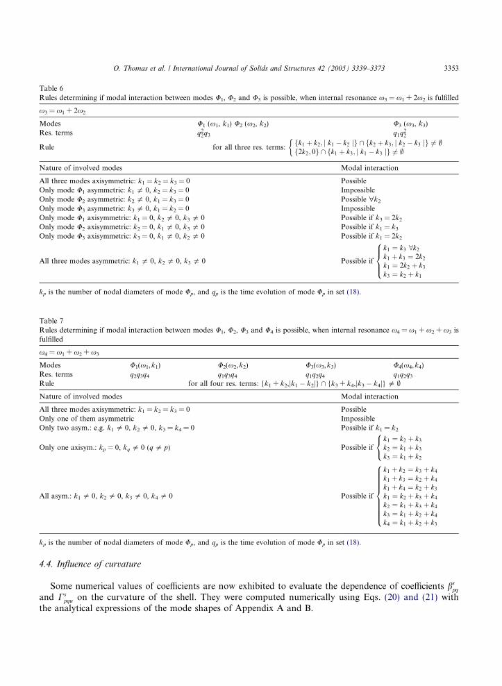
Table 7Rules determining if modal interaction between modes U1, U2, U3 and U4 is possible, when internal resonance x4 = x1 + x2 + x3 isfulfilled
x4 = x1 + x2 + x3
Modes U1(x1,k1) U2(x2,k2) U3(x3,k3) U4(x4,k4)Res. terms q2q3q4 q1q3q4 q1q2q4 q1q2q3
Rule for all four res. terms: {k1 + k2,jk1 � k2j} \ {k3 + k4,jk3 � k4j} 5 ;Nature of involved modes Modal interaction
All three modes axisymmetric: k1 = k2 = k3 = 0 PossibleOnly one of them asymmetric ImpossibleOnly two asym.: e.g. k1 5 0, k2 5 0, k3 = k4 = 0 Possible if k1 = k2
Only one axisym.: kp = 0, kq 5 0 (q5 p) Possible ifk1 ¼ k2 þ k3
k2 ¼ k1 þ k3
k3 ¼ k1 þ k2
8<:
All asym.: k1 5 0, k2 5 0, k3 5 0, k4 5 0 Possible if
k1 þ k2 ¼ k3 þ k4
k1 þ k3 ¼ k2 þ k4
k1 þ k4 ¼ k2 þ k3
k1 ¼ k2 þ k3 þ k4
k2 ¼ k1 þ k3 þ k4
k3 ¼ k1 þ k2 þ k4
k4 ¼ k1 þ k2 þ k3
8>>>>>>>><>>>>>>>>:
kp is the number of nodal diameters of mode Up, and qp is the time evolution of mode Up in set (18).
Table 6Rules determining if modal interaction between modes U1, U2 and U3 is possible, when internal resonance x3 = x1 + 2x2 is fulfilled
x3 = x1 + 2x2
Modes U1 (x1, k1) U2 (x2, k2) U3 (x3, k3)Res. terms q2
2q3 q1q22
Rule for all three res. terms:fk1 þ k2; j k1 � k2 jg \ fk2 þ k3; j k2 � k3 jg 6¼ ;f2k2; 0g \ fk1 þ k3; j k1 � k3 jg 6¼ ;
�
Nature of involved modes Modal interaction
All three modes axisymmetric: k1 = k2 = k3 = 0 PossibleOnly mode U1 asymmetric: k1 5 0, k2 = k3 = 0 ImpossibleOnly mode U2 asymmetric: k2 5 0, k1 = k3 = 0 Possible "k2
Only mode U3 asymmetric: k3 5 0, k1 = k2 = 0 ImpossibleOnly mode U1 axisymmetric: k1 = 0, k2 5 0, k3 5 0 Possible if k3 = 2k2
Only mode U2 axisymmetric: k2 = 0, k1 5 0, k3 5 0 Possible if k1 = k3
Only mode U3 axisymmetric: k3 = 0, k1 5 0, k2 5 0 Possible if k1 = 2k2
All three modes asymmetric: k1 5 0, k2 5 0, k3 5 0 Possible if
k1 ¼ k3 8k2
k1 þ k3 ¼ 2k2
k1 ¼ 2k2 þ k3
k3 ¼ k2 þ k1
8>><>>:
kp is the number of nodal diameters of mode Up, and qp is the time evolution of mode Up in set (18).
O. Thomas et al. / International Journal of Solids and Structures 42 (2005) 3339–3373 3353
4.4. Influence of curvature
Some numerical values of coefficients are now exhibited to evaluate the dependence of coefficients bspq
and Cspqu on the curvature of the shell. They were computed numerically using Eqs. (20) and (21) with
the analytical expressions of the mode shapes of Appendix A and B.
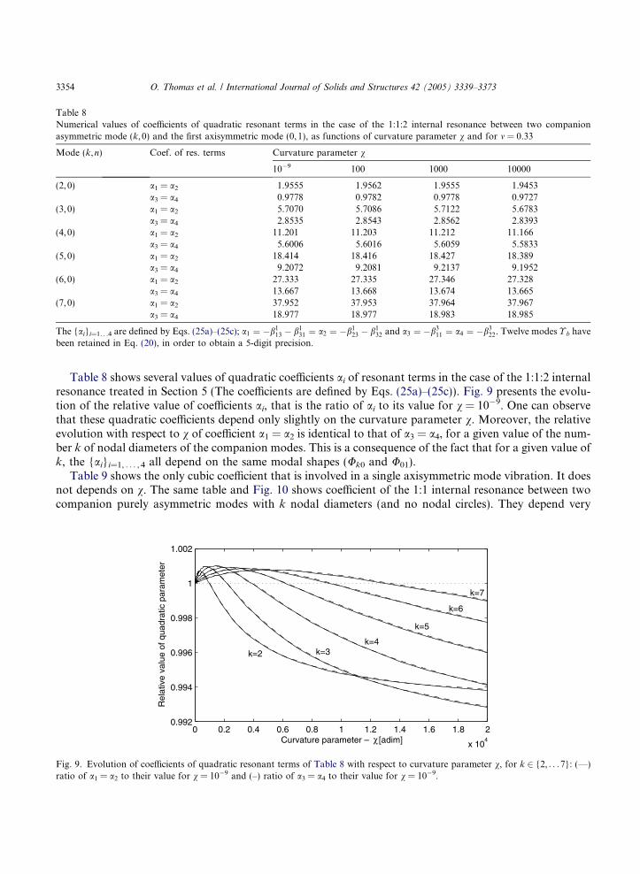
Table 8Numerical values of coefficients of quadratic resonant terms in the case of the 1:1:2 internal resonance between two companionasymmetric mode (k, 0) and the first axisymmetric mode (0,1), as functions of curvature parameter v and for m = 0.33
Mode (k,n) Coef. of res. terms Curvature parameter v
10�9 100 1000 10000
(2,0) a1 = a2 1.9555 1.9562 1.9555 1.9453a3 = a4 0.9778 0.9782 0.9778 0.9727
(3,0) a1 = a2 5.7070 5.7086 5.7122 5.6783a3 = a4 2.8535 2.8543 2.8562 2.8393
(4,0) a1 = a2 11.201 11.203 11.212 11.166a3 = a4 5.6006 5.6016 5.6059 5.5833
(5,0) a1 = a2 18.414 18.416 18.427 18.389a3 = a4 9.2072 9.2081 9.2137 9.1952
(6,0) a1 = a2 27.333 27.335 27.346 27.328a3 = a4 13.667 13.668 13.674 13.665
(7,0) a1 = a2 37.952 37.953 37.964 37.967a3 = a4 18.977 18.977 18.983 18.985
The {ai}i=1. . .4 are defined by Eqs. (25a)–(25c); a1 ¼ �b113 � b1
31 ¼ a2 ¼ �b123 � b1
32 and a3 ¼ �b311 ¼ a4 ¼ �b3
22. Twelve modes � b havebeen retained in Eq. (20), in order to obtain a 5-digit precision.
3354 O. Thomas et al. / International Journal of Solids and Structures 42 (2005) 3339–3373
Table 8 shows several values of quadratic coefficients ai of resonant terms in the case of the 1:1:2 internalresonance treated in Section 5 (The coefficients are defined by Eqs. (25a)–(25c)). Fig. 9 presents the evolu-tion of the relative value of coefficients ai, that is the ratio of ai to its value for v = 10�9. One can observethat these quadratic coefficients depend only slightly on the curvature parameter v. Moreover, the relativeevolution with respect to v of coefficient a1 = a2 is identical to that of a3 = a4, for a given value of the num-ber k of nodal diameters of the companion modes. This is a consequence of the fact that for a given value ofk, the {ai}i=1, . . . , 4 all depend on the same modal shapes (Uk0 and U01).
Table 9 shows the only cubic coefficient that is involved in a single axisymmetric mode vibration. It doesnot depends on v. The same table and Fig. 10 shows coefficient of the 1:1 internal resonance between twocompanion purely asymmetric modes with k nodal diameters (and no nodal circles). They depend very
0 0.2 0.4 0.6 0.8 1 1.2 1.4 1.6 1.8 2
x 104
0.992
0.994
0.996
0.998
1
1.002
k=2 k=3k=4
k=5
k=6
k=7
Curvature parameter – χ [adim]
Rel
ativ
e va
lue
of q
uadr
atic
par
amet
er
Fig. 9. Evolution of coefficients of quadratic resonant terms of Table 8 with respect to curvature parameter v, for k 2 {2, . . .7}: (—)ratio of a1 = a2 to their value for v = 10�9 and (–) ratio of a3 = a4 to their value for v = 10�9.

Table 9Numerical values of coefficients of cubic resonant term in the case of a single axisymmetric mode (0,n) or in the case of the 1:1 internalresonance between two companion asymmetric mode (k, 0), with respect to curvature parameter v and for m = 0.33
Mode (k,n) 10�9 Curvature parameter v
100 1000 10,000
(0,1) 8.5287(0,2) 163.77(0,3) 1076.6(2,0) 1.8966 1.8985 1.9053 1.9093(3,0) 16.984 17.304 17.987 18.121(4,0) 70.001 70.203 71.724 77.034(5,0) 202.83 203.32 207.26 226.33(6,0) 476.77 477.68 485.36 531.57(7,0) 975.31 976.78 989.45 1078.1
Twelve modes � b have been retained in Eq. (21), in order to obtain a five-digit precision.
0 0.2 0.4 0.6 0.8 1 1.2 1.4 1.6 1.8 2
x 104
1
1.02
1.04
1.06
1.08
1.1
1.12
1.14
1.16
1.18
k=2
k=3
k=4
k=5
k=6
k=7
Curvature parameter – χ [adim]
Rel
ativ
e va
lue
of c
ubic
par
amet
er
Fig. 10. Evolution of coefficients of cubic resonant terms of Table 9, related to purely asymmetric modes with k nodal diameters, withrespect to curvature parameter v. The ratio between the coefficient to its value for v = 10�9 is plotted, for k 2 {2, . . .7}.
O. Thomas et al. / International Journal of Solids and Structures 42 (2005) 3339–3373 3355
slightly on the curvature parameter v. The numerical values of this latter case are in agreement with thosecomputed in Touze et al. (2002) for a circular plate.
One can conclude that coefficients are almost constant as a function of v. It is a consequence of the factthat the shell mode shapes slightly depend on curvature, as shown in Section 3.1. Thus, the dependence ofthe dynamics of the shell upon its geometry is mainly governed by the value of eq (Eq. (8b)), since ec is aconstant with respect to the curvature (Eq. (8c)).
5. Application: the case of a one-to-one-to-two internal resonance
This section is devoted to the analysis of a system exhibiting a one-to-one-to-two (1:1:2) internal reso-nance, corresponding to the interaction between two companion asymmetric mode with an axisymmetricmode, whose natural frequency is nearly equal to twice that of the asymmetric ones. This specific internal
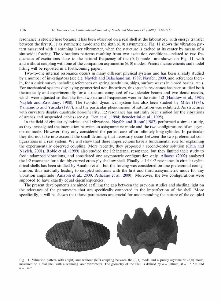
3356 O. Thomas et al. / International Journal of Solids and Structures 42 (2005) 3339–3373
resonance is studied here because it has been observed on a real shell at the laboratory, with energy transferbetween the first (0,1) axisymmetric mode and the sixth (6,0) asymmetric. Fig. 11 shows the vibration pat-tern measured with a scanning laser vibrometer, when the structure is excited at its center by means of asinusoidal forcing. The vibrations patterns resulting from two excitation conditions—related to two fre-quencies of excitations close to the natural frequency of the (0,1) mode—are shown on Fig. 11, withand without coupling with one of the companion asymmetric (6,0) modes. Precise measurements and modelfitting will be reported in a forthcoming paper.
Two-to-one internal resonance occurs in many different physical systems and has been already studiedby a number of investigators (see e.g. Nayfeh and Balachandran, 1989; Nayfeh, 2000, and references there-in, for a quick survey including references on spring pendulum, ships, surface waves in closed basins, etc.).For mechanical systems displaying geometrical non-linearities, this specific resonance has been studied boththeoretically and experimentally for a structure composed of two slender beams and two dense masses,which were adjusted so that the first two natural frequencies were in the ratio 1:2 (Haddow et al., 1984;Nayfeh and Zavodney, 1988). The two-dof dynamical system has also been studied by Miles (1984),Yamamoto and Yasuda (1977), and the particular phenomenon of saturation was exhibited. As structureswith curvature display quadratic non-linearity, 1:2 resonance has naturally been studied for the vibrationsof arches and suspended cables (see e.g. Tien et al., 1994; Benedettini et al., 1995).
In the field of circular cylindrical shell vibrations, Nayfeh and Raouf (1987) performed a similar study,as they investigated the interaction between an axisymmetric mode and the two configurations of an asym-metric mode. However, they only considered the perfect case of an infinitely long cylinder. In particularthey did not take into account the small detuning that necessary occur between the two preferential con-figurations in a real system. We will show that these imperfections have a fundamental role for explainingthe experimentally observed coupling. More recently, they proposed a second-order solution (Chin andNayfeh, 2001). Robie et al. (1999) also studied the 1:2 internal resonance, but they limited their study tofree undamped vibrations, and considered one asymmetric configuration only. Alhazza (2002) analyzedthe 1:2 resonance for a doubly-curved cross-ply shallow shell. Finally, a 1:1:1:2 resonance in circular cylin-drical shells has been studied by Amabili et al., but the forcing was considered on one preferential config-uration, thus naturally leading to coupled solutions with the first and third axisymmetric mode for anyvibration amplitude (Amabili et al., 2000, Pellicano et al., 2000). Moreover, the two configurations weresupposed to have exactly equal eigenfrequencies.
The present developments are aimed at filling the gap between the previous studies and sheding light onthe relevance of the parameters that are specifically connected to the imperfection of the shell. Morespecifically, it will be shown that those parameters are crucial for understanding the nature of the coupled
Fig. 11. Vibration pattern with (right) and without (left) coupling between the (0,1) mode and a purely asymmetric (6,0) mode,measured on a real shell with a scanning laser vibrometer. The geometry of the shell is defined by a = 300mm, R = 1.515m andh = 1mm.
O. Thomas et al. / International Journal of Solids and Structures 42 (2005) 3339–3373 3357
regime. It will be demonstrated that the energy transfer is specific to one of the companion asymmetricmodes and that no traveling wave appear as long as the cubic terms are effectively negligible.
The spherical shell is assumed to be excited by an external sinusoidal force located at its center, whosefrequency X is chosen close to the natural frequency (denoted here by x3) of an axisymmetric mode (0,n 0)of n 0 nodal circles. The curvature parameter v is chosen so that an internal resonance exist between mode(0,n 0) and two companion asymmetric modes (k,n) of frequencies x1 and x2, so that x3 ’ 2x1 ’ 2x2.Fig. 3 shows that these internal resonances occur for many values of v. For example, mode (0,1) can be in-volved in a 1:1:2 internal resonance between any of the asymmetric modes (k, 0) with no nodal circles. In thefollowing, a reduced order model is deduced from the set (18) and we focus on a first-order perturbative solu-tion. As a consequence, (i) only the modes involved in internal resonance are retained, (ii) the cubic terms areneglected with respect to the others, according to the values of the parameters eq and ec (see Table 1) and (iii)all non-resonant terms are dropped. The transverse displacement w(r,h, t) is then written
wðr; h; tÞ ¼ RknðrÞðq1ðtÞ cos kh þ q2ðtÞ sin khÞ þ R0n0q3ðtÞ; ð24Þ
where q1 and q2 are related to the asymmetric modes and q3 to the axisymmetric. Rkn(r) and R0n0 ðrÞ are de-fined in Appendix A. The {qi}i=1,. . .,3 are solutions of the following set, deduced from (18):€q1 þ x21q1 ¼ eq½a1q1q3 � 2l1 _q1 ; ð25aÞ
€q2 þ x22q2 ¼ eq½a2q2q3 � 2l2 _q2 ; ð25bÞ
€q3 þ x23q3 ¼ eq½a3q2
1 þ a4q22 � 2l3 _q3 þ Q cos Xt : ð25cÞ
The forcing terms of the first two oscillators (25a) and (25b) vanish since the corresponding modes have anode at the center of the shell. The term proportional to q2
3 in Eq. (25c) is not considered since it is non-resonant. The reduced-order model defined above is justified because the present study is focused on theloss of stability of the single degree-of-freedom (sdof) solution (defined by the directly excited axisymmetricmode only, q1(t) � q2(t) � 0). A first-order perturbative development is then sufficient and the formalism ofnon-linear normal modes need not to be used (Nayfeh and Nayfeh, 1994). This would not be the case if onewas interested in predicting the hardening or softening behavior of a single mode. In this situation, it wouldbe necessary to retain a number of additional oscillators in the model, the cubic terms as well as the non-resonant terms, as shown for example in the case of circular cylindrical shells by Amabili et al. (1999) or in ageneral case by Touze et al. (2004) with the formalism of non-linear modes.
Coefficients {ai}i=1,. . .,4 can be computed from the bpqs expressed in Eq. (20). In a perfect case, one obtains
a1 = a2, and a3 = a4, as shown in Table 8. However, for the sake of generality, the {ai}i=1,. . .,4 are kept var-iable in the following. To express the internal resonance relationships, we introduce two internal detuningparameters r0 and r1
x2 ¼ x1 þ eqr0; ð26aÞ
x3 ¼ 2x1 þ eqr1: ð26bÞ
One can notice that: x3 = 2x2 + eq(r1 � 2r0). Finally an external detuning parameter r2 is introduced toexpress the nearness of the forcing frequency with the axisymmetric natural frequencyX ¼ x3 þ eqr2: ð27Þ
5.1. Multiple scale solution
System (25) is solved by the method of multiple scales. To the first-order, and for j = 1,2,3
qjðtÞ ¼ qj1ðT 0; T 1Þ þ eqqj2ðT 0; T 1Þ þ Oðe2qÞ; ð28Þ
3358 O. Thomas et al. / International Journal of Solids and Structures 42 (2005) 3339–3373
where T0 = t and T1 = eqt. The first-order equations lead to express the {qj1}j=1,2,3 as
qj1ðT 0; T 1Þ ¼1
2ajðT 1Þ expðihjðT 1ÞÞ expðixjT 0Þ þ c:c:; ð29Þ
where c.c. stands for complex conjugate. Polar form is used to express the amplitude of the first-order solu-tions, which depends on the slow time scale T1. Introducing (29) into the second-order equations leads tothe so-called solvability condition, which can be written as a six-dimensional dynamical system by separat-ing real and imaginary parts. Finally, the following variables allows definition of an autonomous dynamicalsystem:
c1 ¼ r1T 1 þ h3 � 2h1; c2 ¼ ðr1 � 2r0ÞT 1 þ h3 � 2h2; c3 ¼ r2T 1 � h3: ð30Þ
It reads
a01 ¼ �l1a1 þ
a1a1a3
4x1
sin c1; ð31aÞ
c01 ¼ r1 �a3a2
1
4x3a3
cos c1 �a4a2
2
4x3a3
cos c2 �Q
2x3a3
cos c3 þa1a3
2x1
cos c1; ð31bÞ
a02 ¼ �l2a2 þ
a2a2a3
4x2
sin c2; ð31cÞ
c02 ¼ r1 � 2r0 �a3a2
1
4x3a3
cos c1 �a4a2
2
4x3a3
cos c2 �Q
2x3a3
cos c3 þa2a3
2x2
cos c2; ð31dÞ
a03 ¼ �l3a3 �
a3a21
4x3
sin c1 �a4a2
2
4x3
sin c2 þQ
2x3
sin c3; ð31eÞ
c03 ¼ r2 þa3a2
1
4x3a3
cos c1 þa4a2
2
4x3a3
cos c2 þQ
2x3a3
cos c3; ð31fÞ
where (Æ) 0 stands for the derivation with respect to T1.
5.2. Fixed points
Fixed points for Eq. (31) are obtained by cancelling the left-hand side terms, which involve a derivativewith respect to time. There are a priori four kinds of fixed points:
(i) sdof solution. It corresponds to the case where a1 = a2 = 0: no energy transfer between modes occurand the response of the system is governed by the directly excited axisymmetric mode only. Its amplitude isgiven by
a3 ¼Q
2x3
ffiffiffiffiffiffiffiffiffiffiffiffiffiffiffir2
2 þ l23
p ; ð32Þ
(ii) C1 solution. It corresponds to a coupling between the axisymmetric mode and the first asymmetricconfiguration, thus a1 5 0, and a2 = 0.
(iii) C2 solution. The coupling is here with the second asymmetric configuration: a1 = 0, and a2 5 0.(iv) C3 solution. Coupling with both asymmetric configurations at the same time, leading to a1 5 0 and
a2 5 0. It will be shown next that this solution exists only in the perfect case.
O. Thomas et al. / International Journal of Solids and Structures 42 (2005) 3339–3373 3359
Analytical expressions for the C1 and C2 solutions are easily available with a little algebra, which is notreproduced here (see e.g. Nayfeh and Raouf, 1987; Nayfeh and Mook, 1979; Haddow et al., 1984). Onethen obtains:
• C1 solution:
a3 ¼2x1
a1
ffiffiffiffiffiffiffiffiffiffiffiffiffiffiffiffiffiffiffiffiffiffiffiffiffiffiffiffiffiffiffiffiffi4l2
1 þ ðr1 þ r2Þ2q
; ð33aÞ
a1 ¼ 2
ffiffiffiffiffiffiffiffiffiffiffiffiffiffiffiffiffiffiffiffiffiffiffiffiffiffiffiffiffiffiffiffiffiffiffiffiffi�C1 �
ffiffiffiffiffiffiffiffiffiffiffiffiffiffiffiffiffiffiQ2
4a23
� C22
svuut; ð33bÞ
with : C1 ¼2x1x3
a1a3
ð2l1l3 � r2ðr1 þ r2ÞÞ; ð33cÞ
and : C2 ¼2x1x3
a1a3
ð2r2l1 þ l3ðr1 þ r2ÞÞ: ð33dÞ
• C2 solution:
2x2ffiffiffiffiffiffiffiffiffiffiffiffiffiffiffiffiffiffiffiffiffiffiffiffiffiffiffiffiffiffiffiffiffiffiffiffiffiffiffiffiffiffiffiffiffiffi
2q
a3 ¼ a2
4l22 þ ðr1 � 2r0 þ r2Þ ; ð34aÞ
a2 ¼ 2
ffiffiffiffiffiffiffiffiffiffiffiffiffiffiffiffiffiffiffiffiffiffiffiffiffiffiffiffiffiffiffiffiffiffiffiffiffi�C3 �
ffiffiffiffiffiffiffiffiffiffiffiffiffiffiffiffiffiffiQ2
4a24
� C24
svuut; ð34bÞ
with : C3 ¼2x2x3
a2a4
ð2l2l3 � r2ðr1 � 2r0 þ r2ÞÞ; ð34cÞ
and : C4 ¼2x2x3
a2a4
ð2r2l2 þ l3ðr1 � 2r0 þ r2ÞÞ: ð34dÞ
One can notice that the symmetry of the original equations (25) allows derivation of the expression for theC2 solution from the expression found for C1. The symmetry of the system is of great help for the under-standing and analysis of energy transfer, as shown next.
The C3 case is considered by keeping all amplitudes different from zero. However, the operations thatlead to Eqs. (33a) and (34a) are still possible. Thus, in the more general case, when the two asymmetricconfigurations are eventually present in the vibration, a3 can take the two different values given by (33a)and (34a). Moreover it can be shown that if a3 is equal to (33a) (respectively, equal to (34a)), then c2
(respectively, c1) is undefined and a2 = 0 (respectively, a1 = 0) is the only possible case. As a consequence,no other solutions than the ones already described (sdof, C1 and C2) are available, except whenEqs. (33a) and (34a) are simultaneously fulfilled, which is true only in the perfect case (defined by:l1 = l2, a1 = a2, and x1 = x2, which implies r0 = 0). The stability analysis confirms these conclusions,as well as numerical simulations which were conducted with the software DsTool (Guckenheimeret al., 1995).
3360 O. Thomas et al. / International Journal of Solids and Structures 42 (2005) 3339–3373
5.3. Stability analysis
A linear stability analysis is performed by computing the Jacobian matrix J of Eq. (31). We first inves-tigate the stability of the sdof solution. The eigenvalues are
ksdof1;2 ¼ �l3 � ir2; ð35aÞ
kC11 ¼ �l1 þ
a1a3
4x1
sin c1; ð35bÞ
kC12 ¼ � a1a3
2x1
sin c1; ð35cÞ
kC21 ¼ �l2 þ
a2a3
4x2
sin c2; ð35dÞ
kC22 ¼ � a2a3
2x2
sin c2: ð35eÞ
The superscripts indicate that each pair of eigenvalues can be easily related to: (i) the stability of the sdofsolution with respect to perturbations contained within the subspace a1 = a2 = 0 (sdof case), (ii) its stabilitywith respect to perturbations caused by the presence of the first asymmetric configuration (C1 case), (iii) itsstability with respect to perturbations caused by the second asymmetric configuration (C2 case). The simpleform of Eq. (35a–e) is a direct consequence of the relative decoupling and symmetry of the initial equations(25). By forming the products kC1
1 :kC12 and kC2
1 :kC22 , and eliminating c1 and c2 in favor of the other param-
eters, one can exhibit two stability conditions for the sdof solutions:
a3 6 L1ðr2Þ; where L1ðr2Þ ¼2x1
a1
ffiffiffiffiffiffiffiffiffiffiffiffiffiffiffiffiffiffiffiffiffiffiffiffiffiffiffiffiffiffiffiffiffi4l2
1 þ ðr1 þ r2Þ2q
; ð36Þ
a3 6 L2ðr2Þ; where L2ðr2Þ ¼2x2
a2
ffiffiffiffiffiffiffiffiffiffiffiffiffiffiffiffiffiffiffiffiffiffiffiffiffiffiffiffiffiffiffiffiffiffiffiffiffiffiffiffiffiffiffiffiffiffi4l2
2 þ ðr1 � 2r0 þ r2Þ2q
; ð37Þ
with a3 defined by Eq. (32). These stability conditions have been reported in Fig. 12, where the sdof solu-tions is unstable in the gray shaded regions.
In the perfect case—i.e., defined by the complete identity of the two configurations (i.e. a1 = a2, x1 = x2
and l1 = l2), the two curves L1(r2) and L2(r2) are merged. Hence both configurations are simultaneouslyexcited when the sdof curve crosses L1 � L2. It can then be shown that their amplitudes verify the followingrelationship:
a21 þ a2
2 ¼ �4C1 þ
ffiffiffiffiffiffiffiffiffiffiffiffiffiffiffiffiffiffiffiffiffiffiffiffiffiffiffiffiffiffiffiffiffiffiffiffiffiffiffiffiffiffiffiffiffiffiffiffiffiffiffiffiffiffiffiffiffiffiffiffiffiffiffiffiffiffiffiffiffiffiffiffiffiffiffiffiffiffiffiffiffiffiffiffiffiffiffiffiffiffiffiffiffiffiffiffiffiffiffiffiffiffiffiffiffiffi16C2
1 �64x2
1x23
a21a
23
ð4l21 þ ðr1 þ r2Þ2Þðl2
3 þ r22Þ �
4Q2
a23
� �sð38Þ
An infinity of coupled solutions are available: any solution that verify Eq. (38). This has been verifiednumerically. The reader interested in the perfect case is referred to Nayfeh and Raouf (1987) for a completestudy.
In real situations, it is impossible to ensure perfectness, and slight perturbations are always present thatbreak the precedent results and keep the curves L1(r2) and L2(r2) distinct, so that the situation depicted inFig. 12 is generic. The discussion is restricted to positive values of r0, because the ordering of the config-urations is made by their natural frequencies.
The stability of the C1 and C2 solutions is now addressed. In Fig. 12, if the sdof solution is followedfrom r2 < 0 for increasing values, it first crosses L1 at r2 = �1.5, so that a C1 solution is obtained, whose
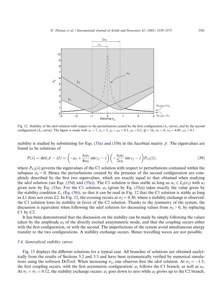
Fig. 12. Stability of the sdof solution with respect to the perturbations caused by the first configuration (L1 curve), and by the secondconfiguration (L2 curve). The figure is made with a1 = 7, a2 = 5, l1 = l3 = 0.1, l2 = 0.2, Q = 16, x1 = 4, x2 = 4.09, x3 = 8.1.
O. Thomas et al. / International Journal of Solids and Structures 42 (2005) 3339–3373 3361
stability is studied by substituting for Eqs. (33a) and (33b) in the Jacobian matrix J. The eigenvalues arefound to be solutions of
P ðkÞ ¼ detðJ� kIÞ ¼ �l2 þa2a3
4x2
sin c2 � k
� �� a2a3
2x2
sin c2 � k
� �PC2ðkÞ; ð39Þ
where PC2(k) governs the eigenvalues of the C1 solution with respect to perturbations contained within thesubspace a2 = 0. Hence the perturbations created by the presence of the second configuration are com-pletely described by the first two eigenvalues, which are exactly equal to that obtained when studyingthe sdof solution (see Eqs. (35d) and (35e)). The C1 solution is thus stable as long as a3 6 L2(r2) with a3
given now by Eq. (33a). For the C1 solution, a3 (given by Eq. (33a)) takes exactly the value given bythe stability condition L1 (Eq. (36)), so that it can be read in Fig. 12 that the C1 solution is stable as longas L1 does not cross L2. In Fig. 12, the crossing occurs at r2 = 0.30, where a stability exchange is observed:the C1 solution loses its stability in favor of the C2 solution. Thanks to the symmetry of the system, thediscussion is equivalent when following the sdof solution for decreasing values from r2 > 0, by replacingC1 by C2.
It has been demonstrated that the discussion on the stability can be made by simply following the valuestaken by the amplitude a3 of the directly excited axisymmetric mode, and that the coupling occurs eitherwith the first configuration, or with the second. The imperfections of the system avoid simultaneous energytransfer to the two configurations. A stability exchange occurs. Hence travelling waves are not possible.
5.4. Generalized stability curves
Fig. 13 displays the different solutions for a typical case. All branches of solutions are obtained analyt-ically from the results of Sections 5.2 and 5.3 and have been systematically verified by numerical simula-tions using the software DsTool. When increasing r2, one observes first the sdof solution. At r2 = �1.5,the first coupling occurs, with the first asymmetric configuration: a1 follows the C1 branch, as well as a3.At r2 ¼ r2 ¼ 0:12, the stability exchange occurs: a1 goes down to zero while a2 grows up to the C2 branch,
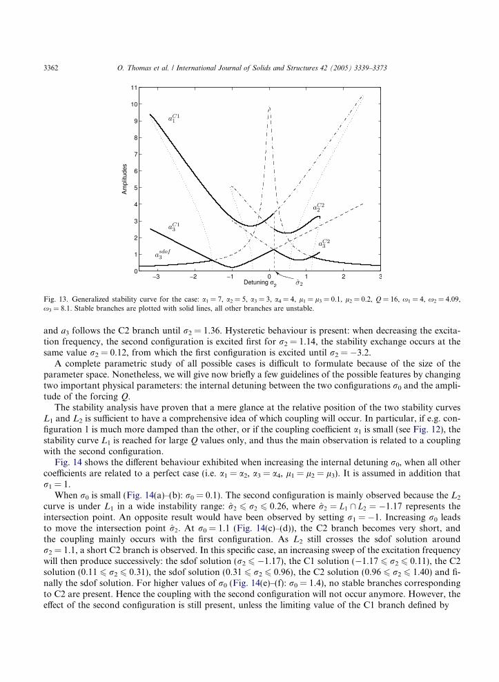
Fig. 13. Generalized stability curve for the case: a1 = 7, a2 = 5, a3 = 3, a4 = 4, l1 = l3 = 0.1, l2 = 0.2, Q = 16, x1 = 4, x2 = 4.09,x3 = 8.1. Stable branches are plotted with solid lines, all other branches are unstable.
3362 O. Thomas et al. / International Journal of Solids and Structures 42 (2005) 3339–3373
and a3 follows the C2 branch until r2 = 1.36. Hysteretic behaviour is present: when decreasing the excita-tion frequency, the second configuration is excited first for r2 = 1.14, the stability exchange occurs at thesame value r2 = 0.12, from which the first configuration is excited until r2 = �3.2.
A complete parametric study of all possible cases is difficult to formulate because of the size of theparameter space. Nonetheless, we will give now briefly a few guidelines of the possible features by changingtwo important physical parameters: the internal detuning between the two configurations r0 and the ampli-tude of the forcing Q.
The stability analysis have proven that a mere glance at the relative position of the two stability curvesL1 and L2 is sufficient to have a comprehensive idea of which coupling will occur. In particular, if e.g. con-figuration 1 is much more damped than the other, or if the coupling coefficient a1 is small (see Fig. 12), thestability curve L1 is reached for large Q values only, and thus the main observation is related to a couplingwith the second configuration.
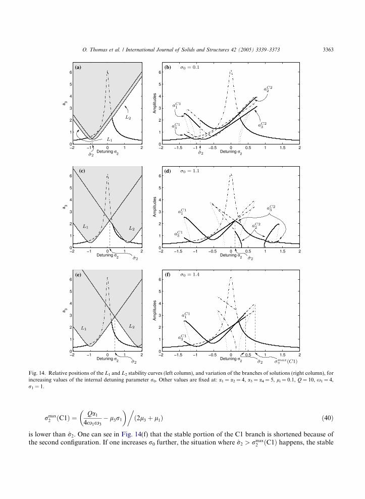
Fig. 14 shows the different behaviour exhibited when increasing the internal detuning r0, when all othercoefficients are related to a perfect case (i.e. a1 = a2, a3 = a4, l1 = l2 = l3). It is assumed in addition thatr1 = 1.
When r0 is small (Fig. 14(a)–(b): r0 = 0.1). The second configuration is mainly observed because the L2
curve is under L1 in a wide instability range: r2 6 r2 6 0:26, where r2 ¼ L1 \ L2 ¼ �1:17 represents theintersection point. An opposite result would have been observed by setting r1 = �1. Increasing r0 leadsto move the intersection point r2. At r0 = 1.1 (Fig. 14(c)–(d)), the C2 branch becomes very short, andthe coupling mainly occurs with the first configuration. As L2 still crosses the sdof solution aroundr2 = 1.1, a short C2 branch is observed. In this specific case, an increasing sweep of the excitation frequencywill then produce successively: the sdof solution (r2 6 �1.17), the C1 solution (�1.17 6 r2 6 0.11), the C2solution (0.11 6 r2 6 0.31), the sdof solution (0.31 6 r2 6 0.96), the C2 solution (0.96 6 r2 6 1.40) and fi-nally the sdof solution. For higher values of r0 (Fig. 14(e)–(f): r0 = 1.4), no stable branches correspondingto C2 are present. Hence the coupling with the second configuration will not occur anymore. However, theeffect of the second configuration is still present, unless the limiting value of the C1 branch defined by
(a)
(c)
(b)
(d)
(e) (f)
Fig. 14. Relative positions of the L1 and L2 stability curves (left column), and variation of the branches of solutions (right column), forincreasing values of the internal detuning parameter r0. Other values are fixed at: a1 = a2 = 4, a3 = a4 = 5, li = 0.1, Q = 10, x1 = 4,r1 = 1.
O. Thomas et al. / International Journal of Solids and Structures 42 (2005) 3339–3373 3363
rmax2 ðC1Þ ¼ Qa1
4x1x3
� l3r1
� ��ð2l3 þ l1Þ ð40Þ
is lower than r2. One can see in Fig. 14(f) that the stable portion of the C1 branch is shortened because ofthe second configuration. If one increases r0 further, the situation where r2 > rmax
2 ðC1Þ happens, the stable
3364 O. Thomas et al. / International Journal of Solids and Structures 42 (2005) 3339–3373
portion of the C1 branch is not shortened and all happens as if only the first configuration was present inthe dynamics.
The variations of the amplitudes of the solutions can be represented as functions of Q in order to high-light the phenomenon of saturation of the directly excited mode. Eq. (33a,b) and (34a,b) are then plottedfor a given r2 and a variable Q. The value r2 ¼ L1 \ L2 which determines the stability exchange, is indepen-dent of Q. Thus for a given external detuning, no stability exchange occurs, so that representation of thiscurves are the same as the already studied 1:2 resonance (see e.g. Nayfeh and Raouf, 1987; Nayfeh andMook, 1979; Haddow et al., 1984).
5.5. Solution for the deflection
In steady state, the deflection of the shell is governed by Eq. (24), with the time functions for the threemodes defined at first-order by
q1ðtÞ ¼ a1 cosX2
t � c1 þ c3
2
� �; ð41aÞ
q2ðtÞ ¼ a2 cosX2
t � c2 þ c3
2
� �; ð41bÞ
q3ðtÞ ¼ a3 cosðXt � c3Þ; ð41cÞ
where ai and ci take the values of a particular stable fixed point. Thus, c3 is the phase difference betweendirectly excited mode q3 and excitation, and c1 and c2 are the phase differences between modes excitedthrough internal resonance on the one hand—respectively q1 and q2—and q3 on the other hand.6. Conclusion
In this paper, a detailed analysis of the non-linear vibrations of thin shallow spherical shells with a freeedge has been proposed. The validity range of the governing equations has been quantified analytically andby comparison with a numerical solution. Then, a method of resolution via projection onto the linearmodes basis has been detailed, hence presenting the general problem including asymmetric vibrations ina uniform manner.
The major set of results is the general non-linear modal interaction rules that have been established,thanks to computation of all coefficients of the non-linear quadratic and cubic terms that appear in the dif-ferential equations. Those coefficients are of major interest as their values govern the energy exchanges be-tween mode that are likely to appear at the non-linear stage. It has been shown that an internal resonancerelation between the natural frequencies of the shell is not a sufficient condition for the non-linear modalinteraction to occur, since some coefficients of the non-linear terms vanish. This is a consequence of therotational symmetry of the geometry of the structure, and coupling rules that hold on the number of nodaldiameters of the involved modes have been derived. It is thus possible to predict if a particular non-linearenergy exchange between modes is possible by considering only the linear modal analysis of the structure:the values of the natural frequencies determine the possible internal resonances and the number of nodaldiameters of the involved modes enable to conclude on the activation of the modal interaction. Finally,an application has been treated: the specific case of a 1:1:2 internal resonance has been revisited, withemphasis on the effect of the slight imperfections of the structure on the energy transfers.
Beyond the important results derived throughout this study, the developed model framework can now beused for studying the rich variety of behaviour exhibited by non-linear shell vibrations. As the results of this
O. Thomas et al. / International Journal of Solids and Structures 42 (2005) 3339–3373 3365
article are based on the rotational symmetry of the structure, similar results can be expected for otheraxisymmetric shells (cylindrical, conical or any profile). An experimental validation of the 1:1:2 internalresonance will be soon reported, showing the validity range and the precision of the model. More generally,this study can serve as a basis for analytical, or numerical-analytical solutions, computations of non-linearnormal modes for prediction of the trend of non-linearity, or, in a different point of view, for analysisand synthesis of the sound produced by musical instruments such as cymbals and gongs (Chaigne et al.,2004).
Acknowledgement
The authors want to thank Eric Luminais for the scrupulous reading of the manuscript he has made.
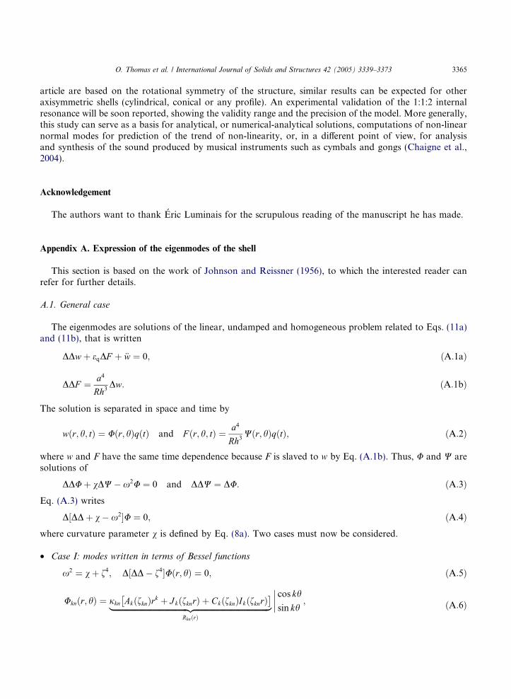
Appendix A. Expression of the eigenmodes of the shell
This section is based on the work of Johnson and Reissner (1956), to which the interested reader canrefer for further details.
A.1. General case
The eigenmodes are solutions of the linear, undamped and homogeneous problem related to Eqs. (11a)and (11b), that is written
DDw þ eqDF þ €w ¼ 0; ðA:1aÞ
DDF ¼ a4
Rh3Dw: ðA:1bÞ
The solution is separated in space and time by
wðr; h; tÞ ¼ Uðr; hÞqðtÞ and F ðr; h; tÞ ¼ a4
Rh3Wðr; hÞqðtÞ; ðA:2Þ
where w and F have the same time dependence because F is slaved to w by Eq. (A.1b). Thus, U and W aresolutions of
DDU þ vDW � x2U ¼ 0 and DDW ¼ DU: ðA:3Þ
Eq. (A.3) writesD½DD þ v � x2 U ¼ 0; ðA:4Þ
where curvature parameter v is defined by Eq. (8a). Two cases must now be considered.• Case I: modes written in terms of Bessel functions
x2 ¼ v þ f4; D½DD � f4 Uðr; hÞ ¼ 0; ðA:5Þ
Uknðr; hÞ ¼ jkn AkðfknÞrk þ JkðfknrÞ þ CkðfknÞIkðfknrÞ� �|fflfflfflfflfflfflfflfflfflfflfflfflfflfflfflfflfflfflfflfflfflfflfflfflfflfflfflfflfflfflfflfflfflfflfflfflfflffl{zfflfflfflfflfflfflfflfflfflfflfflfflfflfflfflfflfflfflfflfflfflfflfflfflfflfflfflfflfflfflfflfflfflfflfflfflfflffl}
RknðrÞ
cos kh
sin kh
"""" ; ðA:6Þ

3366 O. Thomas et al. / International Journal of Solids and Structures 42 (2005) 3339–3373
Wknðr; hÞ ¼ jkn DkðfknÞrk þ 1 þ f4kn
v
� �AkðfknÞ4ðk þ 1Þ r
kþ2 � 1
f2kn
J kðfknrÞ � CkðfknÞIkðfknrÞð Þ" #
cos kh
sin kh
"""" : ðA:7Þ
• Case II: modes written in terms of Kelvin functions
f4 < v; x2 ¼ v � f4; D DD þ f4� �
Uðr; hÞ ¼ 0; ðA:8Þ
Uknðr; hÞ ¼ jkn½AkðfknÞrk þ berkðfknrÞ þ CkðfknÞbeikðfknrÞ |fflfflfflfflfflfflfflfflfflfflfflfflfflfflfflfflfflfflfflfflfflfflfflfflfflfflfflfflfflfflfflfflfflfflfflfflfflfflfflfflffl{zfflfflfflfflfflfflfflfflfflfflfflfflfflfflfflfflfflfflfflfflfflfflfflfflfflfflfflfflfflfflfflfflfflfflfflfflfflfflfflfflffl}RknðrÞ
cos kh
sin kh
"""" ; ðA:9Þ
Wknðr; hÞ ¼ jkn DkðfknÞrk þ 1 � f4kn
v
� �AkðfknÞ4ðk þ 1Þ r
kþ2 þ 1
f2kn
beikðfknrÞ � CkðfknÞberkðfknrÞð Þ" #
cos kh
sin kh
"""" :
ðA:10Þ
In the above equations, Ak, Ck and Dk are constants depending on boundary conditions, jkn is a normal-ization constant, k is the number of nodal diameters and n the number of nodal circles. Jk denotes the Besselfunction of the first kind of order k and Ik(x) = Jk(ix) with i ¼ffiffiffiffiffiffiffi�1
p. Kelvin functions are defined by berk
(x) + ibeik(x) = Jk(i3/2x) = (�1)kIk(i
1/2x). The normalization constant jkn is chosen so that Eq. (22) is ful-filled. Modes Wkn are not normalized (jkn appears in Ukn as well as in Wkn) as they are slaved to transversemodes Ukn.
A.2. Free-edge boundary conditions
Values of f, Ak, Ck and Dk are determined by introducing the boundary conditions. In the case of a free-edge, one obtains in a dimensionless form (see Eqs. (5a)–(5d)):
U and W are bounded at r ¼ 0; ðA:11aÞ
U;rr þ mU;r þ mU;hh ¼ 0 at r ¼ 1; ðA:11bÞ
U;rrr þ U;rr � U;r þ ð2 � mÞU;rhh � ð3 � mÞU;hh ¼ 0 at r ¼ 1; ðA:11cÞ
W;r þ W;hh ¼ 0; W;rh � W;h ¼ 0 at r ¼ 1: ðA:11dÞ
The expressions of the modes in terms of Bessel functions or Kelvin functions depends on the values of k,n and v, results that are summarized in Table A.3.
• Axisymmetric modes and modes with one nodal diameter (k 2 {0,1})The modes express in terms of Bessel functions, so that fkn ¼ fð0Þkn is the nth zero of the equation
DkðfÞ ¼ 0 ðA:12Þ
with Dk defined in Table A.1. This equation is independent of v—and then of curvature—and is theequation with whom are calculated the natural frequencies (denoted by xð0Þkn ¼ fð0Þ2kn ) of the circular plateobtained with v = 0. The natural frequencies of the shell are then, from Eq. (A.5), for all k 2 {0,1} andfor all n
xkn ¼ffiffiffiffiffiffiffiffiffiffiffiffiffiffiv þ f4
kn
q¼
ffiffiffiffiffiffiffiffiffiffiffiffiffiffiffiffiffiffiv þ xð0Þ2
kn
q: ðA:13Þ
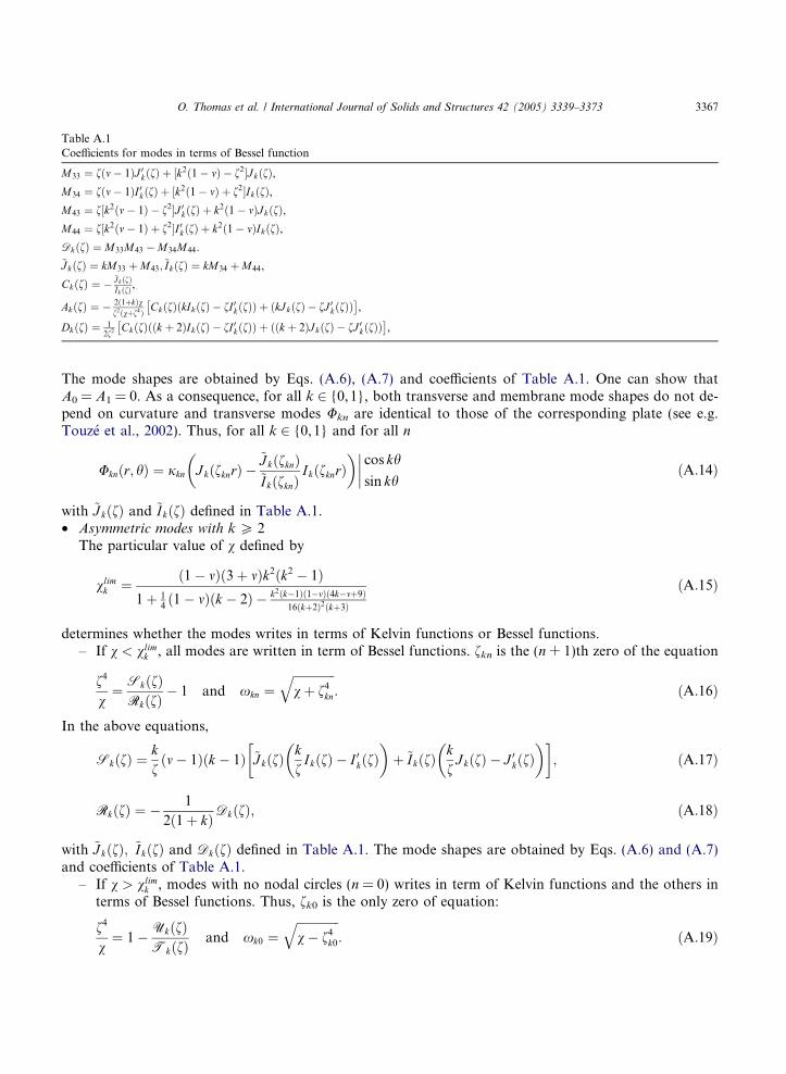
Table A.1Coefficients for modes in terms of Bessel function
M33 ¼ fðm � 1ÞJ 0kðfÞ þ ½k2ð1 � mÞ � f2 JkðfÞ,
M34 ¼ fðm � 1ÞI 0kðfÞ þ ½k2ð1 � mÞ þ f2 IkðfÞ,M43 ¼ f½k2ðm � 1Þ � f2 J 0
kðfÞ þ k2ð1 � mÞJkðfÞ,M44 ¼ f½k2ðm � 1Þ þ f2 I 0kðfÞ þ k2ð1 � mÞIkðfÞ,DkðfÞ ¼ M33M43 �M34M44.
~JkðfÞ ¼ kM33 þM43;~IkðfÞ ¼ kM34 þM44,
CkðfÞ ¼ � ~Jk ðfÞ~Ik ðfÞ
,
AkðfÞ ¼ � 2ð1þkÞvf2ðvþf4Þ CkðfÞðkIkðfÞ � fI 0kðfÞÞ þ ðkJkðfÞ � fJ 0
kðfÞÞ� �
,
DkðfÞ ¼ 12f2 CkðfÞððk þ 2ÞIkðfÞ � fI 0kðfÞÞ þ ððk þ 2ÞJkðfÞ � fJ 0
kðfÞÞ� �
,
O. Thomas et al. / International Journal of Solids and Structures 42 (2005) 3339–3373 3367
The mode shapes are obtained by Eqs. (A.6), (A.7) and coefficients of Table A.1. One can show thatA0 = A1 = 0. As a consequence, for all k 2 {0,1}, both transverse and membrane mode shapes do not de-pend on curvature and transverse modes Ukn are identical to those of the corresponding plate (see e.g.Touze et al., 2002). Thus, for all k 2 {0,1} and for all n
Uknðr; hÞ ¼ jkn J kðfknrÞ �~JkðfknÞ~IkðfknÞ
IkðfknrÞ� �
cos kh
sin kh
"""" ðA:14Þ
with ~JkðfÞ and ~IkðfÞ defined in Table A.1.• Asymmetric modes with k P 2
The particular value of v defined by
vlimk ¼ ð1 � mÞð3 þ mÞk2ðk2 � 1Þ
1 þ 14ð1 � mÞðk � 2Þ � k2ðk�1Þð1�mÞð4k�mþ9Þ
16ðkþ2Þ2ðkþ3Þ
ðA:15Þ
determines whether the modes writes in terms of Kelvin functions or Bessel functions.– If v < vlim
k , all modes are written in term of Bessel functions. fkn is the (n + 1)th zero of the equation
f4
v¼ SkðfÞ
RkðfÞ� 1 and xkn ¼
ffiffiffiffiffiffiffiffiffiffiffiffiffiffiv þ f4
kn
q: ðA:16Þ
In the above equations,
SkðfÞ ¼kfðm � 1Þðk � 1Þ ~JkðfÞ
kfIkðfÞ � I 0kðfÞ
� �þ ~IkðfÞ
kfJkðfÞ � J 0
kðfÞ� �� �
; ðA:17Þ
RkðfÞ ¼ � 1
2ð1 þ kÞDkðfÞ; ðA:18Þ
with ~JkðfÞ; ~IkðfÞ and DkðfÞ defined in Table A.1. The mode shapes are obtained by Eqs. (A.6) and (A.7)and coefficients of Table A.1.
– If v > vlimk , modes with no nodal circles (n = 0) writes in term of Kelvin functions and the others in
terms of Bessel functions. Thus, fk0 is the only zero of equation:
f4
v¼ 1 � UkðfÞ
TkðfÞand xk0 ¼
ffiffiffiffiffiffiffiffiffiffiffiffiffiffiv � f4
k0
q: ðA:19Þ
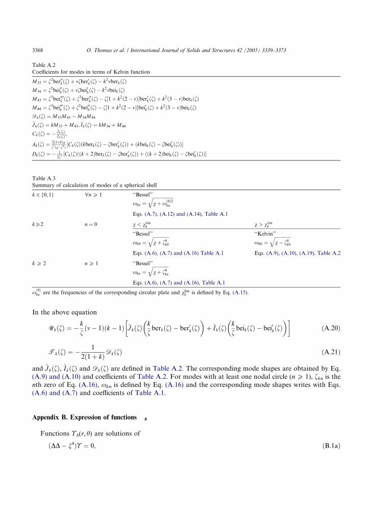
Table A.2Coefficients for modes in terms of Kelvin function
M33 ¼ f2ber00k ðfÞ þ mfber0kðfÞ � k2mberkðfÞM34 ¼ f2bei00k ðfÞ þ mfbei0kðfÞ � k2mbeikðfÞM43 ¼ f3ber000k ðfÞ þ f2ber00k ðfÞ � f½1 þ k2ð2 � mÞ ber0kðfÞ þ k2ð3 � mÞberkðfÞM44 ¼ f3bei000k ðfÞ þ f2bei00k ðfÞ � f½1 þ k2ð2 � mÞ bei0kðfÞ þ k2ð3 � mÞbeikðfÞDkðfÞ ¼ M33M43 � M34M44
~JkðfÞ ¼ kM33 þ M43;~IkðfÞ ¼ kM34 þM44
CkðfÞ ¼ � ~Jk ðfÞ~Ik ðfÞ
,
AkðfÞ ¼ 2ð1þkÞvf2ðv�f4Þ ½CkðfÞðkberkðfÞ � fber0kðfÞÞ þ ðkbeikðfÞ � fbei0kðfÞÞ
DkðfÞ ¼ � 12f2 ½CkðfÞððk þ 2ÞberkðfÞ � fber0kðfÞÞ þ ððk þ 2ÞbeikðfÞ � fbei0kðfÞÞ
Table A.3Summary of calculation of modes of a spherical shell
k 2 {0,1} "n P 1 ‘‘Bessel’’
xkn ¼ffiffiffiffiffiffiffiffiffiffiffiffiffiffiffiffiffiffiv þ xð0Þ2
kn
qEqs. (A.7), (A.12) and (A.14), Table A.1
kP2 n = 0 v < vlimk v > vlim
k
‘‘Bessel’’ ‘‘Kelvin’’
xk0 ¼ffiffiffiffiffiffiffiffiffiffiffiffiffiffiv þ f4
k0
qxk0 ¼
ffiffiffiffiffiffiffiffiffiffiffiffiffiffiv � f4
k0
qEqs. (A.6), (A.7) and (A.16) Table A.1 Eqs. (A.9), (A.10), (A.19), Table A.2
k P 2 n P 1 ‘‘Bessel’’
xkn ¼ffiffiffiffiffiffiffiffiffiffiffiffiffiffiv þ f4
kn
qEqs. (A.6), (A.7) and (A.16), Table A.1
xð0Þkn are the frequencies of the corresponding circular plate and vlim
k is defined by Eq. (A.15).
3368 O. Thomas et al. / International Journal of Solids and Structures 42 (2005) 3339–3373
In the above equation
UkðfÞ ¼ � kfðm � 1Þðk � 1Þ ~JkðfÞ
kfberkðfÞ � ber0kðfÞ
� �þ ~IkðfÞ
kfbeikðfÞ � bei0kðfÞ
� �� �ðA:20Þ
TkðfÞ ¼ � 1
2ð1 þ kÞDkðfÞ ðA:21Þ
and ~JkðfÞ, ~IkðfÞ and DkðfÞ are defined in Table A.2. The corresponding mode shapes are obtained by Eq.(A.9) and (A.10) and coefficients of Table A.2. For modes with at least one nodal circle (n P 1), fkn is thenth zero of Eq. (A.16), xkn is defined by Eq. (A.16) and the corresponding mode shapes writes with Eqs.(A.6) and (A.7) and coefficients of Table A.1.
Appendix B. Expression of functions � b
Functions � b(r,h) are solutions of
ðDD � n4Þ� ¼ 0; ðB:1aÞ
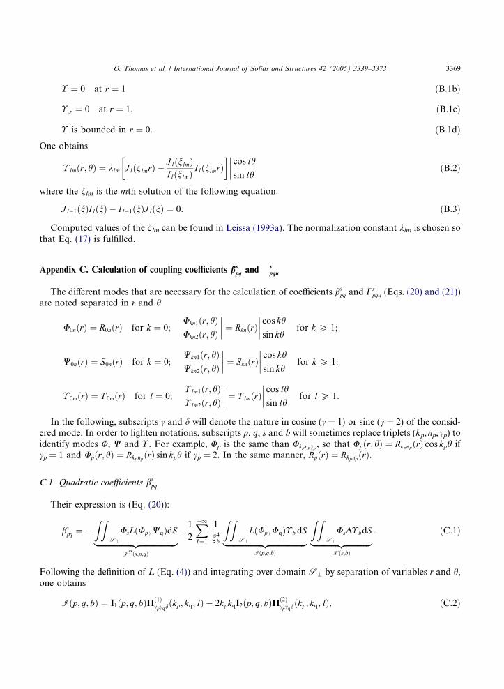
O. Thomas et al. / International Journal of Solids and Structures 42 (2005) 3339–3373 3369
� ¼ 0 at r ¼ 1 ðB:1bÞ
� ;r ¼ 0 at r ¼ 1; ðB:1cÞ
� is bounded in r ¼ 0: ðB:1dÞ
One obtains� lmðr; hÞ ¼ klm J lðnlmrÞ �J lðnlmÞIlðnlmÞ
IlðnlmrÞ� �
cos lh
sin lh
"""" ðB:2Þ
where the nlm is the mth solution of the following equation:
J l�1ðnÞIlðnÞ � Il�1ðnÞJ lðnÞ ¼ 0: ðB:3Þ
Computed values of the nlm can be found in Leissa (1993a). The normalization constant klm is chosen sothat Eq. (17) is fulfilled.
Appendix C. Calculation of coupling coefficients bspq and � s
pqu
The different modes that are necessary for the calculation of coefficients bspq and Cs
pqu (Eqs. (20) and (21))are noted separated in r and h
U0nðrÞ ¼ R0nðrÞ for k ¼ 0;Ukn1ðr; hÞUkn2ðr; hÞ
"""" ¼ RknðrÞcos kh
sin kh
"""" for k P 1;
W0nðrÞ ¼ S0nðrÞ for k ¼ 0;Wkn1ðr; hÞWkn2ðr; hÞ
"""" ¼ SknðrÞcos kh
sin kh
"""" for k P 1;
� 0mðrÞ ¼ T 0mðrÞ for l ¼ 0;� lm1ðr; hÞ� lm2ðr; hÞ
"""" ¼ T lmðrÞcos lh
sin lh
"""" for l P 1:
In the following, subscripts c and d will denote the nature in cosine (c = 1) or sine (c = 2) of the consid-ered mode. In order to lighten notations, subscripts p, q, s and b will sometimes replace triplets (kp,np,cp) toidentify modes U, W and � . For example, Up is the same than Ukpnpcp , so that Upðr; hÞ ¼ RkpnpðrÞ cos kph ifcp = 1 and Upðr; hÞ ¼ RkpnpðrÞ sin kph if cp = 2. In the same manner, RpðrÞ ¼ RkpnpðrÞ.
C.1. Quadratic coefficients bspq
Their expression is (Eq. (20)):
bspq ¼ �
ZZS?
UsLðUp;WqÞdS|fflfflfflfflfflfflfflfflfflfflfflfflfflfflfflfflfflffl{zfflfflfflfflfflfflfflfflfflfflfflfflfflfflfflfflfflffl}JWðs;p;qÞ
� 1
2
Xþ1
b¼1
1
n4b
ZZS?
LðUp;UqÞ� b dS|fflfflfflfflfflfflfflfflfflfflfflfflfflfflfflfflfflffl{zfflfflfflfflfflfflfflfflfflfflfflfflfflfflfflfflfflffl}Iðp;q;bÞ
ZZS?
UsD� bdS|fflfflfflfflfflfflfflfflfflfflfflffl{zfflfflfflfflfflfflfflfflfflfflfflffl}Kðs;bÞ
: ðC:1Þ
Following the definition of L (Eq. (4)) and integrating over domain S? by separation of variables r and h,one obtains
Iðp; q; bÞ ¼ I1ðp; q; bÞPð1Þcpcqdðkp; kq; lÞ � 2kpkqI2ðp; q; bÞPð2Þ
cpcqdðkp; kq; lÞ; ðC:2Þ
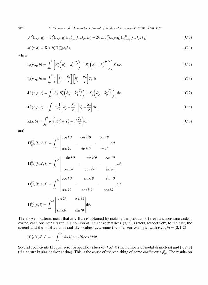
3370 O. Thomas et al. / International Journal of Solids and Structures 42 (2005) 3339–3373
JWðs; p; qÞ ¼ JW1 ðs; p; qÞPð1Þ
cscpcqðks; kp; kqÞ � 2kpkqJ
W2 ðs; p; qÞPð3Þ
cscpcqðks; kp; kqÞ; ðC:3Þ
Kðs; bÞ ¼ Kðs; bÞPð4Þcsdðs; bÞ; ðC:4Þ
where
I1ðp; q; bÞ ¼Z 1
0
R00p R0
q � k2q
Rq
r
� �þ R00
q R0p � k2
p
Rp
r
� �� �T bdr; ðC:5Þ
I2ðp; q; bÞ ¼Z 1
0
1
rR0
p �Rp
r
� �R0
q �Rq
r
� �T bdr; ðC:6Þ
JW1 ðs; p; qÞ ¼
Z 1
0
Rs R00p S0
q � k2q
Sq
r
� �þ S00
q R0p � k2
p
Rp
r
� �� �dr; ðC:7Þ
JW2 ðs; p; qÞ ¼
Z 1
0
Rs1
rR0
p �Rp
r
� �S0
q �Sq
r
� �dr; ðC:8Þ
Kðs; bÞ ¼Z 1
0
Rs rT 00b þ T 0
b � l2 T b
r
� �dr ðC:9Þ
and
Pð1Þcc0dðk; k
0; lÞ ¼Z 2p
0
cos kh cos k0h cos lh
sin kh sin k0h sin lh
""""""""""""""dh;
Pð2Þcc0dðk; k
0; lÞ ¼Z 2p
0
� sin kh � sin k0h cos lh
cos kh cos k0h sin lh
""""""""""""""dh;
Pð3Þcc0dðk; k0; lÞ ¼
Z 2p
0
cos kh � sin k0h � sin lh
sin kh cos k0h cos lh
""""""""""""""dh;
Pð4Þcd ðk; lÞ ¼
Z 2p
0
cos kh cos lh
sin kh sin lh
""""""""""""""dh:
The above notations mean that any Pcc0d is obtained by making the product of three functions sine and/orcosine, each one being taken in a column of the above matrices. (c,c 0,d) refers, respectively, to the first, thesecond and the third column and their values determine the line. For example, with (c,c 0,d) = (2,1,2)
Pð3Þ212ðk; k0; lÞ ¼ �
Z 2p
0
sin kh sin k0h cos lhdh:
Several coefficients P equal zero for specific values of (k,k 0, l) (the numbers of nodal diameters) and (c,c 0,d)(the nature in sine and/or cosine). This is the cause of the vanishing of some coefficients bs
pq. The results on

Table C.1Conditions on modes Up, Uq, Us and � b that lead to non-zero Iðp; q; bÞ, Kðs; bÞ and JWðs; p; qÞJWðs; p; qÞ 6¼ 0 Iðp; q; bÞ 6¼ 0 Kðs; bÞ 6¼ 0+ + +ks 2 {kp + kq,jkp � kqj} l 2 {kp + kq,jkp � kqj} l = ks
Us,cs Up,cp Uq,cq,Wq,cq Up,cp Uq,cq � b,d Us,cs � b,d
cos,1 cos,1 cos,1 cos,1 cos,1 cos,1 cos,1 cos,1sin,2 sin,2 sin,2 sin,2 sin,2 sin,2
sin,2 cos,1 sin,2 sin,2 cos,1 sin,2sin,2 cos,1 cos,1 sin,2
O. Thomas et al. / International Journal of Solids and Structures 42 (2005) 3339–3373 3371
Iðp; q; bÞ, Kðs; bÞ and JWðs; p; qÞ are summarized in Table C.1. To obtain a non-zero bspq, one must have
either JWðs; p; qÞ 6¼ 0 or at least one mode � b so that Iðp; q; bÞKðs; bÞ 6¼ 0. It is summarized in Table 2.
C.2. Cubic coefficients Cspqu
Their expression is (Eq. (20)):
TableCondit
Iðp; q+l 2 fk
Up,cp
cos,1sin,2sin,2cos,1
Cspqu ¼
1
2
Xþ1
b¼1
1
n4b
Z ZS
LðUp;UqÞ� bdS|fflfflfflfflfflfflfflfflfflfflfflfflfflfflfflfflfflffl{zfflfflfflfflfflfflfflfflfflfflfflfflfflfflfflfflfflffl}Iðp;q;bÞ
Z ZS
UsLðUu; � bÞdS|fflfflfflfflfflfflfflfflfflfflfflfflfflfflfflfflfflffl{zfflfflfflfflfflfflfflfflfflfflfflfflfflfflfflfflfflffl}J� ðs;u;bÞ
; ðC:10Þ
where Iðp; q; bÞ has been calculated in the above section and J� ðs; u; bÞ has the same structure thanJWðs; p; qÞ and writes
J� ðs; u; bÞ ¼ J�1 ðs; u; bÞPð1Þcs;cu;d
ðks; ku; lÞ � 2kulJ�2 ðs; u; bÞP
ð3Þcs;cu;d
ðks; ku; lÞ; ðC:11Þ
where
J�1 ðs; u; bÞ ¼Z 1
0
Rs R00u T 00
b � l2 T b
r
� �þ T 00
b R0u � k2
u
Ru
r
� �� �dr; ðC:12Þ
J�2 ðs; s; bÞ ¼Z 1
0
Rs1
rR0
u �Ru
r
� �T 0
b �T b
r
� �dr: ðC:13Þ
Again, non-zero Cspqu are obtained if Iðp; q; bÞJ� ðs; u; bÞ 6¼ 0, cases specified in Table C.2. The conse-
quences on Cspqu are summarized in Table 2.
C.2ions on modes Up, Uq, Us, Uu and � b that lead to non-zero Iðp; q; bÞ and J!ðs; p; qÞ
; bÞ 6¼ 0
p þ kq; j kp � kq jg
J� ðs; u; bÞ 6¼ 0+l 2 fks þ ku; j ks � ku jg
Uq,cq � b,d Us, cs Uu,cu � b,d
cos,1 cos,1 cos,1 cos,1 cos,1sin,2 sin,2 sin,2cos,1 sin,2 sin,2 cos,1 sin,2sin,2 cos,1 sin,2
3372 O. Thomas et al. / International Journal of Solids and Structures 42 (2005) 3339–3373
References
Alhazza, K.A., 2002. Nonlinear vibrations of doubly curved cross-ply shallow shells. Ph.D. Thesis, Virginia Polytechnic Institute andState University.
Amabili, M., Paıdoussis, M.P., 2003. Review of studies on geometrically nonlinear vibrations and dynamics of circular cylindricalshells and panels, with and without fluid–structure interaction. ASME Appl. Mech. Rev. 56 (4), 349–381.
Amabili, M., Pellicano, R., Paıdoussis, M.P., 1998. Nonlinear vibrations of simply supported circular cylindrical shells, coupled toquiescent fluid. J. Fluids Struct. 12, 883–918.
Amabili, M., Pellicano, F., Paıdoussis, M.P., 1999. Non-linear dynamics and stability of circular cylindrical shells containing flowingfluid, part II: large-amplitude vibrations without flow. J. Sound Vib. 228 (5), 1103–1124.
Amabili, M., Pellicano, F., Vakakis, A.F., 2000. Nonlinear vibrations and multiple resonances of fluid-filled, circular shells, part 1:equations of motion and numerical results. ASME J. Vib. Acoust. 122, 346–354.
Benedettini, F., Rega, G., Alaggio, R., 1995. Non-linear oscillations of a four-degree-of-freedom model of a suspended cable undermultiple internal resonance conditions. J. Sound Vib. 182 (5), 775–798.
Chaigne, A., Touze, C., Thomas, O., 2004. Mechanical models of musical instruments and sound synthesis: the case of gongs andcymbals. In: Proceedings of the International Symposium on Musical Acoustics. Nara, Japan.
Chin, C.-M., Nayfeh, A.H., 2001. A second-order approximation of multi-modal interactions in externally excited circular cylindricalshells. Nonlinear Dynam. 26, 45–66.
Chu, H.-N., Herrmann, G., 1956. Influence of large amplitudes on free flexural vibrations of rectangular elastic plates. J. Appl. Mech.23, 532–540.
Donnell, L.H., 1934. A new theory for the buckling of thin cylinders under axial compression and bending. Trans. Am. Soc. Mech.Eng. 56, 795–806.
Efstathiades, G.J., 1971. A new approach to the large-deflction vibrations of imperfect circular disks using Galerkin�s procedure. J.Sound Vib. 16 (2), 231–253.
Evensen, D.A., Fulton, R.E., oct 1965. Some studies on the nonlinear dynamic response of shell-type structures. Tech. Rep. TMX56843, NASA Langley Research Center.
Evensen, H.A., Evan-Iwanowsky, R.M., 1967. Dynamic response and stability of shallow spherical shells subject to time-dependantloading. AIAA J. 5 (5), 969–976.
Goncalves, P.B., 1994. Axisymmetric vibrations of imperfect shallow spherical caps under pressure loading. J. Sound Vib. 174 (2), 249–260.
Grossman, P.L., Koplik, B., Yu, Y.-Y., 1969. Nonlinear vibrations of shallow spherical shells. ASME J. Appl. Mech 39E, 451–458.Guckenheimer, J., Holmes, P., 1983. Nonlinear Oscillations, Dynamical Systems and Bifurcations of Vector Fields. Springer-Verlag,
New York.Guckenheimer, J., Myers, M., Wicklin, F., Worfolk, P., 1995. Dstool: a dynamical system toolkit with an interactive graphical
interface. Technical Report, Center for Applied Mathematics, Cornell University.Haddow, A.G., Barr, A.D.S., Mook, D.T., 1984. Theoretical and experimental study of modal interaction in a two-degree-of-freedom
structure. J. Sound Vib. 97, 451–473.Hamdouni, A., Millet, O., 2003. Classification of thin shell models deduced from the nonlinear three-dimensional elasticity, part I: the
shallow shells. Arch. Mech. 55 (2), 135–175.Hui, D., 1983. Large-amplitude vibrations of geometrically imperfect shallow spherical shells with structural damping. AIAA J. 21
(12), 1736–1741.Johnson, M.W., Reissner, E., 1956. On transverse vibrations of shallow spherical shells. Quart. Appl. Math. 15 (4), 367–380.Kalnins, A., 1964. Effect of bending on vibrations of spherical shells. J. Acoust. Soc. Am. 36 (1), 74–81.Koiter, W.T., 1965. On the nonlinear theory of thin elastic shells, part I, II and III. Proc. Kon. Neth. Akad. Wet. B69, 1–54.Lacarbonara, W., Rega, G., Nayfeh, A.H., 2003. Resonant non-linear normal modes, part I: analytical treatment for structural one-
dimensional systems. Int. J. Non-Linear Mech. 38, 851–872.Lee, W.K., Yeo, M.H., Samoilenko, S.B., 2003. The effect of the number of nodal diameters on non-linear interactions in two
asymmetric vibration modes of a circular plate. J. Sound. Vib 268 (5), 1013–1023.Leissa, A.W., 1993a. Vibration of plates. Acoustical Society of America (original issued NASA SP-160, 1969).Leissa, A.W., 1993b. Vibration of shells. Acoustical Society of America (original issued NASA SP-288, 1973).Leissa, A.W., Kadi, A.S., 1971. Curvature effects on shallow shell vibrations. J. Sound. Vib. 16 (2), 173–187.Lobitz, D.W., Nayfeh, A.H., Mook, D.T., 1977. Non-linear analysis of vibrations of irregular plates. J. Sound. Vib. 50 (2), 203–217.Marguerre, K., 1938. Zur Theorie der Gekrummten Platte Grosser Formanderung. In: Proceedings of the 5th International Congress
on Applied Mechanics, pp. 93–101.Miles, J.W., 1984. Resonantly forced motion of two quadratically coupled oscillators. Physica D 13, 247–260.Morand, H.J.-P., Ohayon, R., 1995. Fluid Structure Interaction. John Wiley and Sons, New York.
O. Thomas et al. / International Journal of Solids and Structures 42 (2005) 3339–3373 3373
Moussaoui, F., Benamar, R., 2002. Non-linear vibrations of shell-type structures: a review with bibliography. J. Sound. Vib. 255 (1),161–184.
Mushtari, K.M., Galimov, K.Z., 1961. Non-linear theory of thin elastic shells. Israel Program for Scientific Translations (Russian ed.,1957).
Nayfeh, A.H., 2000. Nonlinear interactions: analytical, computational and experimental methods. In: Wiley Series in NonlinearScience, New York.
Nayfeh, A.H., Balachandran, B., 1989. Modal interactions in dynamical and structural systems. ASME Appl. Mech. Rev. 42 (11), 175–201.
Nayfeh, A.H., Mook, D.T., 1979. Nonlinear Oscillations. John Wiley and Sons Inc, New York.Nayfeh, A.H., Nayfeh, J.F., Mook, D.T., 1992. On methods for continuous systems with quadratic and cubic nonlinearities. Nonlinear
Dynam. 3, 145–162.Nayfeh, A.H., Nayfeh, S.A., 1994. On nonlinear modes of continuous systems. J. Vib. Acoust. 116, 129–136.Nayfeh, A.H., Raouf, R.A., 1987. Non-linear oscillations of circular cylindrical shells. Int. J. Solids Struct. 23 (12), 1625–1638.Nayfeh, A.H., Zavodney, L.D., 1988. Experimental observation of amplitude and phase-modulated responses of two internally
coupled oscillators to a harmonic excitation. ASME J. Appl. Mech. 55, 706–710.Pellicano, F., Amabili, M., Vakakis, A.F., 2000. Nonlinear vibrations and multiple resonances of fluid-filled, circular shells, part 2:
perturbation analysis. ASME J. Vib. Acoust. 122, 355–364.Qatu, M.S., 2002. Recent research advances in the dynamic behavior of shells: 1989–2000, part 2: homogeneous shells. ASME Appl.
Mech. Rev. 55 (5), 415–434.Raman, A., Mote Jr., C.D., 2001. Effects of imperfection on the non-linear oscillations of circular plates spinning near critical speed.
Int. J. Non-linear Mech. 36, 261–289.Robie, F.M., Popov, A.A., Thompson, J., 1999. Auto-parametric resonance in cylindrical shells using geometric averaging. J. Sound
Vib. 227 (1), 65–84.Soedel, W., 1981. Vibrations of Shells and Plates. Marcel-Dekker Inc., New York.Sridhar, S., Mook, D.T., Nayfeh, A.H., 1975. Non-linear resonances in the forced responses of plates, part I: symmetric responses of
circular plates. J. Sound Vib. 41 (3), 359–373.Sridhar, S., Mook, D.T., Nayfeh, A.H., 1978. Non-linear resonances in the forced responses of plates, part II: asymmetric responses of
circular plates. J. Sound Vib. 59 (2), 159–170.Thomas, O., Touze, C., Chaigne, A., Sep. 2001. Non-linear behavior of gongs through the dynamic of simple rods systems. In:
Proceedings of the International Symposium on Musical Acoustics, Perugia, Italy, pp. 173–178.Tien, W.M., Namachchivaya, N.S., Bajaj, A.K., 1994. Non-linear dynamics of as shallow arch under periodic excitation, I: 1:2 internal
resonance. Int. J. Nonlinear Mech. 29 (3), 349–366.Tobias, S.A., Arnold, R.N., 1957. The influence of dynamical imperfection on the vibration of rotating disks. Proc. of the Instn. of
Mech. Eng. 171, 669–690.Touze, C., Thomas, O., 2004. Reduced-order modeling for a cantilever beam subjected to harmonic forcing. In: proc. of EUROMECH
Colloquium 457: nonlinear modes of vibrating systems. Frejus, France, pp. 165–168.Touze, C., Thomas, O., Chaigne, A., 2002. Asymmetric non-linear forced vibrations of free-edge circular plates, part 1: theory. J.
Sound. Vib. 258 (4), 649–676.Touze, C., Thomas, O., Chaigne, A., 2004. Hardening/softening behaviour in nonlinear oscillations of structural systems using non-
linear normal modes. J. Sound. Vib. 273 (1–2), 77–101.Verpeaux, P., Charras, T., Millard, A., 1988. Calcul des structures et intelligence artificielle. Pluralis, ed., Paris, http://www-
cast3m.cea.fr, Chapter CASTEMCASTEM 2000: Une approche moderne du calcul des structures.Yamamoto, T., Yasuda, K., 1977. On the internal resonance in a non-linear two-degree-of-freedom system. Bull. Jpn. Soc. Mech. Eng.
20, 168–175.Yasuda, K., Kushida, G., 1984. Nonlinear forced oscillations of a shallow spherical shell. Bull. JSME 27 (232), 2233–2240.Ye, Z.M., 1997. The non-linear vibration and dynamic instability of thin shallow shells. J. Sound Vib. 202 (3), 303–311.Yeo, M.H., Lee, W.K., 2002. Corrected solvability conditions for non-linear asymmetric vibrations of a circular plate. J. Sound. Vib
257 (4), 653–665.