non-local solution of mixed integral equation with ... · non-local solution of mixed integral...
TRANSCRIPT

© 2015. M. A. Abdou, S. A. Raad & W. Wahied. This is a research/review paper, distributed under the terms of the Creative Commons Attribution-Noncommercial 3.0 Unported License http://creativecommons.org/licenses/by-nc/3.0/), permitting all non commercial use, distribution, and reproduction in any medium, provided the original work is properly cited.
Global Journal of Science Frontier Research: F Mathematics and Decision Sciences Volume 15 Issue 7 Version 1.0 Year 2015 Type : Double Blind Peer Reviewed International Research Journal Publisher: Global Journals Inc. (USA) Online ISSN: 2249-4626 & Print ISSN: 0975-5896
Non-Local Solution of Mixed Integral Equation with Singular Kernel
By M. A. Abdou, S. A. Raad & W. Wahied Alexandria University, Egypt
Abstract- In this paper, we consider a non-local mixed integral equation in position and time in the space 2 L 1,1 C 0,T ;T. Then, using a quadratic numerical method, we have a system of Fredholm integral equations (SFIEs), where the existence of a unique solution is considered. Moreover, we consider Product Nystrom method (PNM), as a famous method to solve the singular integral equations, to obtain an algebraic system. Finally, some numerical results are considered, and the error estimate, in each case, is computed.
Keywords: non-local solution, fredholm-volterra integral equation, system of fredholm integral equations, weakly kernel, algebraic system.
GJSFR-F Classification : 45B05, 45G10, 60R
NonLocalSolutionofMixedIntegralEquationwithSingularKernel
Strictly as per the compliance and regulations of :

Non-Local Solution of Mixed Integral Equation with Singular Kernel
M. A. Abdou α, S. A. Raad σ & W. Wahied ρ
non-local solution, fredholm-volterra integral equation, system of fredholm integral equations, weakly kernel, algebraic system.
I.
Introduction
57
Globa
lJo
urna
lof
Scienc
eFr
ontie
rResea
rch
V
olum
eXV Issue
er
sion
IV
VII
Yea
r20
15
© 2015 Global Journals Inc. (US)
F)
)
Authorα: Department of Mathematics, Faculty of Education Alexandria University Egypt. e-mail: [email protected],Author σ: Department of Mathematics, Faculty Applied Sciences, Umm Al– Qura University. e-mail: [email protected], Author ρ: Department of Mathematics, Faculty of Science, Damanhour University Egypt. e-mail: [email protected]
Abstract- In this paper, we consider a non-local mixed integral equation in position and time in the space . Then, using a quadratic numerical method, we have a system of Fredholm integral
equations (SFIEs), where the existence of a unique solution is considered. Moreover, we consider Product Nystrom method (PNM), as a famous method to solve the singular integral equations, to obtain an algebraic system. Finally, some numerical results are considered, and the error estimate, in each case, is computed.
2 1,1 0, ; 1L C T T
The integral equations have received considerable interest of many applications in different mathematical areas of sciences. Therefore, the authors established many analytic and numeric methods to obtain the solutions of the integral equations. For some works, the reader can for-ward to the following references [1-5]. For the analytical methods, one can use degenerate kernel method, Cauchy method (singular integral method), Laplace transformation method, Fourier transformation method, potential theory method, and Krien’s method. More infor-mation for the analytic methods can be found in Muskhelishvili [6], Popov [7], Tricomi [8], Hochstad [9] and Green [10]. More recently, since analytical methods on practical problems often fail, numerical solutions of these equations are much studied subjected of numerous works. The interested reader should consult the fine exposition by Atkinson [11], Delves and Mohamed [12], Golberg [13] and Linz [14] for some different numerical methods. In [15] a mixed integral equation in one-dimensional is considered, under certain conditions, and the solution in a series form is obtained. In addition, a mixed integral equation of the second kind, when the Fredholm kernel takes a logarithmic form is discussed and solved in [16]. In [17] Kauthen used a collection method to solve the mixed integral equation with continuous kernel, numerically. Consider the mixed integral equation of the second kind:
1
1 0
, ( , ) , , , , , .t
x t f x y H x t x t k x y y t dy F t x d
(1)
Ref
6.N
. I. M
usk
hel
ishvili, S
ingu
lar
Inte
gral
Equat
ions,
Noo
rdhof
f (1
953)
.
Keywords:

Non-Local Solution of Mixed Integral Equation with Singular Kernel
© 2015 Global Journals Inc. (US)
58
Globa
lJo
urna
lof
Scienc
eFr
ontie
rResea
rch
V
olum
eYea
r20
15
F
)
)
XV Issue
er
sion
IV
VII
The given two continuous function ( , )f x y and , , ,H x t x t define in the Banachspace 2 1,1 0, ,L C T 0 1,t T where the first function is called the free term and the second function is known as the memory of the integral equation. The known functions k x y and ,F t represent the kernels of Fredholm and Volterra integral terms, respec-
tively. The unknown function ,x t represents the solution of (1).The constant may be complex, has a physical meaning and , defines the kind of integral equation. In order to guarantee the existence and uniqueness solution of Eq.(1), we assume the follow-ing conditions:
(i) The given function , , ,H x t x t with its partial derivatives with respect to position and time is continuous in the space 2 0,L C T , for the constant 1L L and 2L L satisfies the following conditions:
1 2( . ) , , , L , ( . ) , , , , , , L , ,i a H x t x t x t i b H x t x t H x t x t x t x t
Where the norm is defined as
1/212
00 1
, max , .t
t Tx t x dx d
(ii) The Fredholm kernel satisfies 1 1
2 2
1 1
,k x y dydx M
( M is a constant).
(iii) The discontinuous function ( )F t is absolutely integrable with respect to for all
0 1t T , and satisfies 0
( )t
F t d N ( N is constant).
(iv) The given function ( , )f x t with its partial derivatives with respect to position x and time
t are continuous in the space 2[ 1,1] [0, ]L C T and its norm is defined as
121
2
00 1
( , ) max ( , ) cos tan .t
t Tf x t f x dx d V t
,
If the conditions (i) – (iii) are satisfied, then Eq. (1) has a
solution ,x t in the space 2 1,1 0,L C T inside the sphere of radius such that:
/ [ L ], LV M TN M TN . ◘ (2)
In the remainder, of this paper a suitable quadratic numerical method is used to reduce the mixed integral equation into SFIEs of the second kind. Then using PNM, as a suitable numer-ical method to solve the singular integral equations, the SFIEs will reduce to an algebraic sys-tem. Finally, many numerical results are calculated when the kernel takes a logarithmic form and Carleman function forms. Moreover, the error estimate, in each case, is computed.
a) Theorem 1 (without proof):
unique
In this section, a quadratic numerical method is used; see Atkinson [11], Delves and Mohamed [12], to obtain SFIEs of the second kind, where the existence and uniqueness of the integral
II. System of Fredholm Integral Equations
11.K.
E.
Atk
inson
, A
Surv
ey of
Num
erical M
ethod
for
the
Solu
tion of
Fred
holm
In
tegral Equation
of the S
econd K
ind, S
IAM
, Philad
elphia, 1976.
Ref
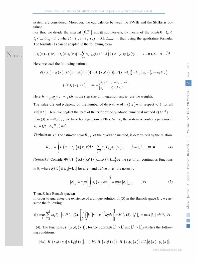
For this, we divide the interval 0,T into m subintervals, by means of the points 00 t
1 ... mt t T , where , , , 0,1,2,...,i jt t t i j m , then using the quadrature formula. The formula (1) can be adapted in the following form
11
,0 1
( ) , , 0,1,2,..., .i
i i i i i j i j j i
j
x f x H x x F x k x y y dy i m
(3)
Here, we used the following nations:
, , , , , , ;i i i i i ix t x H x t x t H x x , ,; ,i j i j i i i iF t t F F
2 0,
, ; .0
j
i i jj
h j j if x t f x
h j i
Here, 10max ( ),i j j i
j mh t t h
is the step size of integration, and j are the weights,
The value of i and p depend on the number of derivative of ,v t with respect to t for all
0,T . Here, we neglect the term of the error of the quadratic numerical method 10 .pih
If in (3) , ,i i iF we have homogeneous SFIEs. While, the system is nonhomogeneous if
,( ) 0.i i i iF
The estimate error , ,m iR of the quadratic method, is determined by the relation
, ,00
, , 1,2,...,t i
m i i j j i j j
j
R F t t x d F x i m
.◘ (4)
Consider 0 1, ,..., ,...ix x x x be the set of all continuous functions
in E, where 2[ 1,1]i x L for all i , and define on E the norm by
2
12 21
1
max max , .i iE Li ix dx i
(5)
Then, E is a Banach space.◘In order to guarantee the existence of a unique solution of (3) in the Banach space E , we as-sume the following:
Definition 1:
Remark1:
system are considered. Moreover, the equivalence between the F-VIE and the SFIEs is ob-tained.
1 11 2 2
,0 1 1
(1). max , (2). , (3). max *, .i
j i j iEj ij
F N k x y dydx M f f V i
(4). The functions ,i iH x x , for the constants 1 L L and 2
L L satisfies the follow-ing conditions:
1(4. ). , Li i ia H x x x , 2(4. ). , , Li i i i i ib H x x H x x x x .
Non-Local Solution of Mixed Integral Equation with Singular Kernel
59
Globa
lJo
urna
lof
Scienc
eFr
ontie
rResea
rch
V
olum
eXV Issue
er
sion
IV
VII
Yea
r20
15
© 2015 Global Journals Inc. (US)
F)
)
Notes

The SFIEs (4) have a unique solution i x in the Banach E under the conditions:
** / [1 ]; min .ii
V N M L ◘ (6)
In this section, we discuss the numerical solution of Eq. (3), when the kernel of position has a singular term, using PNM, see [11, 12].For this, write the singular kernel of (3) in the form
( ) ( , )k x y k x y x y
Where, ( )k x y is a badly behavior, while ( , )x y well behavior.
In view of (7), the SFIEs (3), can be adapted in the form
1
, , , , , , , , ,0 0
, 1,2,..., .i N
i i p i p i p i p j i j j p p q p q i q
j q
f H F w i N
Where, we use the following definitions , , ,; ,i p i p i p i p i p i px H x x H :
, 1( , ) 1 , 0,1,...,p q p q p px x x y ph p N with 21 ,
Nh N even.
In addition, the weight terms ,p qw are given by, see [12],
,0 ,1 ,2 1 , 1 ,2 , 1 , , 2, -2 , , .p p p q p q p q pq p q p N p Nw w w w (9)
2 21 1
, 2 2 1 , 2 2 10 0
21
, 2 2 10
1 ( ( ) ) , 1 2 ( ( ) ) ,2 2
2 ( ( ) ) .2
p q p q p q p q
p q p q
h hk y y h d k y y h d
hk y y h d
Here, in (9), we introduce the change of variable 2 2 1, 0 2qy y h
The relation between the estimate local error ,N qR and Eq. (8) is
b) Theorem 2 (without proof): space
III. Product Nystrom Method
Definition 2:
1
, , ,01
,N
N q i pq p q i q
q
R k x y y dy w
.◘ (10)
The PNM is said to be convergent of order r in the interval 1,1 , if and only if for sufficiently large N , there exists a constant 0s independent of N such that
r
i i Nx x sN
.◘ (11)
In order to guarantee the existence of unique solution of the NAS (8) in the Banach space , we assume the following conditions:
Definition 3:
Non-Local Solution of Mixed Integral Equation with Singular Kernel
© 2015 Global Journals Inc. (US)
60
Globa
lJo
urna
lof
Scienc
eFr
ontie
rResea
rch
V
olum
eYea
r20
15
F
)
)
XV Issue
er
sion
IV
VII
.12.L
.M
. Delv
es and J
.L. M
oham
ed, C
omputation
al Meth
ods for In
tegral Equation
s, P
hila
-delp
hia, 1985
.
Ref
(7)
(8)

1* *
, , , , 1 1,0 0
( )max ; ( ) sup ; ( ) sup ( , , constants).i N
j i j p q p q i pj q i pj q
a F N b w c c f f V N V c
(d) For the constants 1L L and 2L L , , ,i p i pH satisfies the conditions:
, , 1 , , , , , 2 , ,( .1) L , ( .2) L .i p i p i p i p i p i p i p i p i pd H d H H
The NAS (8) has a unique solution ,i p in the space
,,
; sup ,i pi p
under the following conditions
*, / [ * L ]; min .i p i
iV N c ◘ (12)
The equivalence between the NAS (8) and the SFIEs (3) is satisfies if:
1
, , 10 1
, ( ).N
p q p q i i
q
w qh k x y y dy N
Under the conditions of theorem3, the sequence of functions, , ,N i pN
of (10) convergence uniformly to the solution ,i p of (3) in the space .
From Eq. (8), we write
1
, , , , , , , , ,0
, , , ,0
1
.
i
i p i p i p i p i p i p j i j j p j pN N Nji
N
p q p q i q i q Nq
H H F
w
(13)
Using the conditions (a-d) of theorem 3, and using condition (3) of theorem 2, the above ine-
quality can be adapted in the form
, ,,
Lsup , 1.i p i p N
Ni p
N c
a) Theorem3 (without proof):
Theorem 4:
Proof:
Hence, we have 0N
as .N ◘
The estimate total error of PNM, , , ,m N m i N qR R R of Eq.(1) is determined by the following relation
1
, , , , , ,0 01 0
, , , ,t N i
m N p q p q i q j i j j p
q j
R k x y y t dy F t x d w F
. (14)
Definition 4:
●The equivalence between the NAS and F-VIE:
When ,m N , the sum
1
, , ,0 0 1 0
, , , .tN i
pq p q i q j ij j p
q j
w v k x y y t dy F t x d
Non-Local Solution of Mixed Integral Equation with Singular Kernel
61
Globa
lJo
urna
lof
Scienc
eFr
ontie
rResea
rch
V
olum
eXV Issue
er
sion
IV
VII
Yea
r20
15
© 2015 Global Journals Inc. (US)
F)
)
Notes

Then the solution of the NAS (8) becomes the solution of F-VIE (1).
if the conditions (i) and (ii) of theorem1 are satisfied, then the sequence of func-
tions , , ,m N m N x t convergence uniformly to the exact solution ,x t of Eq.
(1)) in the space 2[ 1,1] 0,L C T .
the formula (1) with its approximation solution gives
1
, , ,1
,0
, , , , , , , ,
( , ) , , .
m N m N m N
t
m N
H x t x t H x t x t k x y y t y t dy
F t x x d
(19)
Using , ,F t N ,F t is continuous, then with the aid of conditions (i-2), (ii) then, apply-
ing Cauchy Schwarz inequality, the above inequality becomes
, , 2, L 1m N m N NT M .
Hence, we have 2
, 0,0m N L C T
as ,m N .
the total error ,m NR satisfies ,,lim 0m N
m NR
.
Assume the NF-VIE of the second kind:
( ) ( ) ( ( )) ∫ (| |)
( ) ∫ ( )
( )
Where the kernel of Fredholm term has Carleman (| |) | |
and
Logarithmic (| |) | | kernel, the historical function ( ( )) take a
linear form ( ) , and a nonlinear form ( ) , the kernel of Volterra term ( )
IV. Applications
Theorem 5:
Proof:
Corollary 2:
and the exact solution : ( ) Applying PNM, the results are ob-tained numerically by Maple 12 software, for , with . The interval [ ] is divided into unites.
When the singular kernel takes the Carleman function form
(| |) | |
( ( )) ( ),
Application 1:
Case 1:
Here, the integral equation (1) takes the linear form
( ) ( ) ( ) ∫ (| |)
( ) ∫ ( )
( ) ( )
Non-Local Solution of Mixed Integral Equation with Singular Kernel
© 2015 Global Journals Inc. (US)
62
Globa
lJo
urna
lof
Scienc
eFr
ontie
rResea
rch
V
olum
eYea
r20
15
F)
)
XV Issue
er
sion
IV
VII
Notes

X EX.
APP ERR APP ERR APP ERR
-1 6.400E-07 6.400E-07 0.000E+00 6.400E-07 4.000E-16 6.400E-07 5.000E-16-0.8 4.096E-07 4.096E-07 1.000E-16 4.096E-07 3.000E-16 4.096E-07 2.000E-16-0.6 2.304E-07 2.304E-07 3.000E-16 2.304E-07 2.000E-16 2.304E-07 1.000E-16-0.4 1.024E-07 1.024E-07 1.000E-16 1.024E-07 0.000E-00 1.024E-07 1.000E-16-0.2 2.560E-08 2.560E-08 5.000E-17 2.560E-08 4.000E-17 2.560E-08 1.000E-17
0 0.000E-00 5.200E-18 5.200E-18 2.200E-18 2.200E-18 -7.400E-18 7.400E-180.2 2.560E-08 2.560E-08 3.000E-17 2.560E-08 2.000E-17 2.560E-08 2.000E-170.4 1.024E-07 1.024E-07 1.000E-16 1.024E-07 0.000E-00 1.024E-07 1.000E-160.6 2.304E-07 2.304E-07 3.000E-16 2.304E-07 2.000E-16 2.304E-07 1.000E-160.8 4.096E-07 4.096E-07 0.000E+00 4.096E-07 0.000E-00 4.096E-07 0.000E+00
1 6.400E-07 6.400E-07 3.000E-16 6.400E-07 3.000E-16 6.400E-07 5.000E-16
Table (1)
(1-ii) T=0.05
X EX. APP ERR APP ERR APP ERR
-1 2.500E-03 2.500E-03 5.000E-12 2.500E-03 6.000E-12 2.500E-03 4.000E-12-0.8 1.600E-03 1.600E-03 2.000E-12 1.600E-03 4.000E-12 1.600E-03 2.000E-12-0.6 9.000E-04 9.000E-04 1.800E-12 9.000E-04 1.600E-12 9.000E-06 8.910E-12-0.4 4.000E-04 4.000E-04 9.000E-13 4.000E-04 8.000E-13 4.000E-04 8.000E-13-0.2 1.000E-04 1.000E-04 2.000E-13 1.000E-04 2.000E-13 1.000E-04 3.000E-13
0 0.000E+00 3.060E-14 3.060E-14 3.160E-14 3.160E-14 3.450E-14 3.450E-140.2 1.000E-04 1.000E-04 2.000E-13 1.000E-04 2.000E-13 1.000E-04 3.000E-130.4 4.000E-04 4.000E-04 9.000E-13 4.000E-04 1.000E-12 4.000E-04 7.000E-130.6 9.000E-04 9.000E-04 1.900E-12 9.000E-04 1.700E-12 9.000E-04 1.500E-120.8 1.600E-03 1.600E-03 3.000E-12 1.600E-03 3.000E-12 1.600E-03 2.000E-12
1 2.500E-03 2.500E-03 5.000E-12 2.500E-03 6.000E-12 2.500E-03 4.000E-12
Table (2)
(1-iii) T=0.8
X EX.
APP ERR APP ERR APP ERR
-1 0.64 0.64006387 6.38739E-05 0.640063922 6.39213E-05 0.640063992 6.39914E-05
-0.8 0.4096 0.409641023 4.10232E-05 0.409641088 4.10877E-05 0.409641183 4.11831E-05
-0.6 0.2304 0.230423216 2.32163E-05 0.230423263 2.32632E-05 0.230423329 2.33291E-05
-0.4 0.1024 0.10241049 1.04902E-05 0.102410519 1.05193E-05 0.102410558 1.05578E-05
-0.2 2.56E-02 2.56E-02 2.85211E-06 2.56E-02 2.86893E-06 2.56E-02 2.88919E-06
0 0 3.06E-07 3.05785E-07 3.18E-07 3.18284E-07 3.32E-07 3.32246E-07
0.2 2.56E-02 2.56E-02 2.85211E-06 2.56E-02 2.86892E-06 2.56E-02 2.88918E-06
0.4 0.1024 0.10241049 1.04901E-05 0.102410519 1.05191E-05 0.102410558 1.05577E-05
0.6 0.2304 0.230423217 2.32164E-05 0.230423263 2.32633E-05 0.230423329 2.33293E-05
0.8 0.4096 0.409641023 4.10228E-05 0.409641088 4.10877E-05 0.409641183 4.11832E-05
1 0.64 0.640063874 6.38738E-05 0.640063922 6.39213E-05 0.640063992 6.39915E-05
Table (3)
(1-i) T=0.0008
Non-Local Solution of Mixed Integral Equation with Singular Kernel
63
Globa
lJo
urna
lof
Scienc
eFr
ontie
rResea
rch
V
olum
eXV Issue
er
sion
IV
VII
Yea
r20
15
© 2015 Global Journals Inc. (US)
F)
)
Notes

X EX.
APP ERR APP ERR APP ERR-1 6.400E-07 6.351E-07 4.901E-09 6.344E-07 5.620E-09 6.333E-07 6.680E-09
-0.8 4.096E-07 4.043E-07 5.290E-09 4.033E-07 6.263E-09 4.019E-07 7.688E-09-0.6 2.304E-07 2.253E-07 5.085E-09 2.246E-07 5.781E-09 2.236E-07 6.753E-09-0.4 1.024E-07 9.757E-08 4.828E-09 9.715E-08 5.249E-09 9.660E-08 5.804E-09-0.2 2.560E-08 2.096E-08 4.640E-09 2.073E-08 4.875E-09 2.045E-08 5.153E-09
0 0.000E+00 4.573E-09 4.573E-09 4.742E-09 4.742E-09 4.925E-09 4.925E-090.2 2.560E-08 2.096E-08 4.640E-09 2.073E-08 4.874E-09 2.045E-08 5.152E-090.4 1.024E-07 9.758E-08 4.823E-09 9.716E-08 5.241E-09 9.661E-08 5.792E-090.6 2.304E-07 2.253E-07 5.064E-09 2.247E-07 5.748E-09 2.237E-07 6.708E-090.8 4.096E-07 4.044E-07 5.233E-09 4.034E-07 6.176E-09 4.020E-07 7.573E-091 6.400E-07 6.354E-07 4.563E-09 6.350E-07 4.959E-09 6.345E-07 5.485E-09
Table (4)
(2-ii) T=0.05
X EX.
APP ERR APP ERR APP ERR-1 2.5E-03 2.481E-03 1.905E-05 2.478E-03 2.185E-05 2.474E-03 2.597E-05
-0.8 1.6E-03 1.579E-03 2.060E-05 1.576E-03 2.439E-05 1.570E-03 2.994E-05-0.6 9.0E-04 8.802E-04 1.983E-05 8.775E-04 2.254E-05 8.737E-04 2.633E-05-0.4 4.0E-04 3.812E-04 1.885E-05 3.795E-04 2.049E-05 3.773E-04 2.265E-05-0.2 1.0E-04 8.188E-05 1.812E-05 8.096E-05 1.904E-05 7.988E-05 2.012E-05
0 0.0E+00 1.786E-05 1.786E-05 1.853E-05 1.853E-05 1.924E-05 1.924E-050.2 1.0E-04 8.188E-05 1.812E-05 8.096E-05 1.904E-05 7.988E-05 2.012E-050.4 4.0E-04 3.812E-04 1.882E-05 3.795E-04 2.046E-05 3.774E-04 2.261E-050.6 9.0E-04 8.803E-04 1.975E-05 8.776E-04 2.241E-05 8.738E-04 2.616E-050.8 1.6E-03 1.580E-03 2.038E-05 1.576E-03 2.405E-05 1.571E-03 2.949E-05
1 2.5E-03 2.482E-03 1.774E-05 2.481E-03 1.928E-05 2.479E-03 2.132E-05
Table (5)
(2-iii) T=0.8
-0.6 0.2304 0.22693220 0.00346780 0.226453153 0.003946847 0.225783412 0.004616588-0.4 0.1024 0.09838890 0.00401110 0.098036574 0.004363426 0.097572594 0.004827406-0.2 2.56E-02 2.12E-02 0.00443337 2.09E-02 0.004658686 2.07E-02 0.004925819
0 0 4.60E-03 0.00459856 4.77E-03 0.004769697 4.95E-03 0.0049540650.2 2.56E-02 2.12E-02 0.00443282 2.09E-02 0.004657871 2.07E-02 0.0049247440.4 0.1024 0.09839359 0.00400641 0.098043649 0.004356351 0.097582076 0.0048179240.6 0.2304 0.22694706 0.00345294 0.226475929 0.003924072 0.225814449 0.0045855510.8 0.4096 0.40675174 0.00284827 0.406231277 0.003368724 0.405460083 0.004139917
1 0.64 0.63803898 0.00196103 0.637865533 0.002134467 0.637635663 0.002364338
X EX.
APP ERR APP ERR APP ERR
-1 0.64 0.63788999 0.00211002 0.637573604 0.002426397 0.637107531 0.00289247
-0.8 0.4096 0.40671993 0.00288007 0.406183063 0.003416937 0.405396058 0.004203942
When the non-local term is nonlinear ( ( )) ( )
(2-i) T=0.0008
Case 2:
Table (6)
Non-Local Solution of Mixed Integral Equation with Singular Kernel
© 2015 Global Journals Inc. (US)
64
Globa
lJo
urna
lof
Scienc
eFr
ontie
rResea
rch
V
olum
eYea
r20
15
F
)
)
XV Issue
er
sion
IV
VII
Notes

When the singular kernel takes the logarithmic function
(| |) | |
Case 3: ( ( )) ( )
XT=0.0008 T=0.05 T=0.8
EX APP ERR EX APP ERR EX APP ERR-1 6.400E-07 6.400E-07 6.000E-16 2.5E-03 2.500E-03 4.000E-12 6.400E-01 0.64006336 6.33562E-05
-0.8 4.096E-07 4.096E-07 2.000E-16 1.6E-03 1.600E-03 2.000E-12 4.096E-01 0.40964041 4.04056E-05-0.6 2.304E-07 2.304E-07 3.000E-16 9.0E-04 9.000E-04 1.000E-12 2.304E-01 0.23042266 2.26594E-05-0.4 1.024E-07 1.024E-07 1.000E-16 4.0E-04 4.000E-04 7.000E-13 1.024E-01 0.10241001 1.00122E-05-0.2 2.560E-08 2.560E-08 0.000E-00 1.0E-04 1.000E-04 0.000E+00 2.560E-02 2.56E-02 2.43323E-06
0 0.000E-00 3.605E-18 3.605E-18 0.0E+00 2.703E-15 2.703E-15 0.000E-00 9.17E-08 9.17299E-080.2 2.560E-08 2.560E-08 1.000E-17 1.0E-04 1.000E-04 7.000E-14 2.560E-02 2.56E-02 2.43325E-060.4 1.024E-07 1.024E-07 2.000E-16 4.0E-04 4.000E-04 5.000E-13 1.024E-01 0.10241001 1.00122E-050.6 2.304E-07 2.304E-07 0.00E+00 9.0E-04 9.000E-04 1.000E-12 2.304E-01 0.23042266 2.26595E-050.8 4.096E-07 4.096E-07 1.000E-16 1.6E-03 1.600E-03 3.000E-12 4.096E-01 0.40964041 4.04057E-051 6.400E-07 6.400E-07 5.000E-16 2.5E-03 2.500E-03 4.000E-12 6.400E-01 0.64006336 6.33562E-05
Table (7)
( ( )) ( )
XT=0.0008 T=0.05 T=0.8
EX APP ERR EX APP ERR EX APP ERR
-1 6.400E-07 6.388E-07 1.189E-09 2.500E-03 2.495E-03 4.621E-06 6.400E-01 6.395E-01 4.816E-04-0.8 4.096E-07 4.084E-07 1.229E-09 1.600E-03 1.595E-03 4.785E-06 4.096E-01 4.090E-01 6.464E-04-0.6 2.304E-07 2.300E-07 4.412E-10 9.000E-04 8.983E-04 1.720E-06 2.304E-01 2.301E-01 2.804E-04-0.4 1.024E-07 1.029E-07 4.730E-10 4.000E-04 4.018E-04 1.846E-06 1.024E-01 1.028E-01 4.066E-04-0.2 2.560E-08 2.675E-08 1.149E-09 1.000E-04 1.045E-04 4.487E-06 2.560E-02 2.670E-02 1.097E-03
0 0.000E+00 1.394E-09 1.394E-09 0.000E+00 5.447E-06 5.447E-06 0.00E+00 1.394E-03 1.394E-030.2 2.560E-08 2.675E-08 1.149E-09 1.000E-04 1.045E-04 4.487E-06 2.560E-02 2.670E-02 1.097E-030.4 1.024E-07 1.029E-07 4.730E-10 4.000E-04 4.018E-04 1.846E-06 1.024E-01 1.028E-01 4.066E-040.6 2.304E-07 2.300E-07 4.412E-10 9.000E-04 8.983E-04 1.720E-06 2.304E-01 2.301E-01 2.804E-040.8 4.096E-07 4.084E-07 1.229E-09 1.600E-03 1.595E-03 4.785E-06 4.096E-01 4.090E-01 6.464E-041 6.400E-07 6.388E-07 1.189E-09 2.500E-03 2.495E-03 4.621E-06 6.400E-01 6.395E-01 4.816E-04
Table (8)
●The non-local term is called the histories of the problem and is considered with negative sign
Application 2:
Case 4:
V. Conclusions
I- For the Carleman kernel (| |) | | and for the linear non- local term
( ( )) ( ) e have E. Max. and E.Min. respectively, the following:
(i) In Table (1) at T=0.0008: for are ,respectively3.000E-16 , 0.000E-00. While
are 4.000E-16 and 0.000E-00. Finally at are 5.000E-16 and 0.000E-00.
(ii) In Table (2) at T=0.005: for 5.000E-12 and 2.000E-13. For are 6.000E-12 and
1.000E-12. While are 8.910E-12 and 3.450E-14.
(iii) In Table (3) at T=0.8: for 6.38738E-05 and 3.05785E-07; for are 6.39213E-05
and 1.05193E-05. Finally for are 6.39914E-05 and 1.05577E-05.
Non-Local Solution of Mixed Integral Equation with Singular Kernel
65
Globa
lJo
urna
lof
Scienc
eFr
ontie
rResea
rch
V
olum
eXV Issue
er
sion
IV
VII
Yea
r20
15
© 2015 Global Journals Inc. (US)
F)
)
Notes

II- For the Carleman kernel and nonlinear non- local term ( ( )) ( )
(iv) In Table (4) at T=0.0008: for we obtain 5.290E-09, 4.563E-09. Also,
we get 6.263E-09and 4.742E-09. Finally for we have 7.688E-09and 4.925E-09.
(v) In Table (5) at T=0.005: for 2.060E-05and 1.774E-05. For are 2.439E-05and
1.853E-05. For are 2.994E-05 and 1.924E-05.
(vi) In Table (6) at T=0.8: for 0.00459856 and 0.00196103; for are 0.004769697and
0.002134467. For are 0.004954065and 0.002364338.
III- For a logarithmic kernel (| |) | | and linear non- local term ( ( ))
( ) E. Max. and E. Min are given respectively, as the following:
(vii) In Table (7) at T=0.0008:, we have 6.000E-16 and 0.000E-00. At T=0.005 we have 4.000E-12;
0.000E-00. At T=0. 8, 6.33562E-05, 9.17299E-08.
IV- For a logarithmic and non linear non- local term ( ( )) ( )
the E. Max. and E.Min are respectively,
(viii) In Table (8) at T=0.0008:, we have 1.229E-09 and 4.412E-10. At T=0.005
5.447E-06; 1.720E-06. At T=0. 8, 4.816E-04, 1.097E-03.
From the above results, we deduce that the error in the linear non- local function is less than
the error in the nonlinear case. This result is true, where the integral equation without non-
local term in the linear case.
References Références
Referencias
1. C. Constanda, Integral equation of the first kind in plane elasticity, J.Quart. Appl. Math. Vol. LIII No. 4(1995) 783-793.
2. E. Venturing, The Galerkin method for singular integral equations revisited. J. Comp. Appl. Math. Vol. 40 (1992) 91-103.
3. R. Kangro, P. Oja, Convergence of spline collection for Volterra integral equation, Appl. Num. Math. 58(2008)1434-1447.
4. T. Diego, P. Lima, Super convergence of collocation methods for class of weakly singular integral equations, J. Cam. Appl. Math. 218 (2008) 307-316.
5. G. A. Anastasia, A. Aral, Generalized Picard singular integrals, Compute. Math. Appl. 57 (2009) 821-830.
6. N. I. Muskhelishvili, Singular Integral Equations, Noordhoff (1953).7. G. Ya. Popov, Contact problems for a linearly deformable base, Kiev, Odessa
(1982)].8. F. G. Tricomi, Integral equations, N.Y. (1985). 9. H. Hochstadt, Integral equations, N.Y. London (1971).10. C. D. Green, Integral equation methods, N.Y. (1969).11. K. E. Atkinson, A Survey of Numerical Method for the Solution of Fredholm
Integral Equation of the Second Kind, SIAM, Philadelphia, 1976. 12. L. M. Delves and J.L. Mohamed, Computational Methods for Integral Equations,
Phila-delphia, 1985. 13. M. A. Golberg, Numerical Solution of Integral Equation, Plenum, N. Y. 1990.
Non-Local Solution of Mixed Integral Equation with Singular Kernel
© 2015 Global Journals Inc. (US)
66
Globa
lJo
urna
lof
Scienc
eFr
ontie
rResea
rch
V
olum
eYea
r20
15
F
)
)
XV Issue
er
sion
IV
VII
Notes

14. P. Linz, Analytical and Numerical methods for Volterra equations, SIAM, Philadelphia, 1985).
15. M. A. Abdou, Fredholm – Volterra equation of the first kind and contact problem, Appl. Math. Compute. 125 (2002) 177 -193.
16. M. A. Abdou, Fredholm integral equation with potential kernel and its structure resolvent, Appl. Math. Compute. 107 (2000) 169-180.
17. J. P. Kauthen, Continuous time collection for Volterra-Fredholm integral equations, Numerische Math. 56 (1989) 409-424.
Non-Local Solution of Mixed Integral Equation with Singular Kernel
67
Globa
lJo
urna
lof
Scienc
eFr
ontie
rResea
rch
V
olum
eXV Issue
er
sion
IV
VII
Yea
r20
15
© 2015 Global Journals Inc. (US)
F)
)
Notes

This page is intentionally left blank
© 2015 Global Journals Inc. (US)
68
Globa
lJo
urna
lof
Scienc
eFr
ontie
rResea
rch
V
olum
eYea
r20
15
F
)
)
XV Issue
er
sion
IV
VII
Non-Local Solution of Mixed Integral Equation with Singular Kernel