non-peripheral ideal decompositions of alternating...
TRANSCRIPT
NON-PERIPHERAL IDEAL DECOMPOSITIONS OF ALTERNATING KNOTS
STAVROS GAROUFALIDIS, IAIN MOFFATT, AND DYLAN P. THURSTON
Abstract. An ideal triangulation T of a hyperbolic 3-manifold M with one cusp is non-peripheralif no edge of T is homotopic to a curve in the boundary torus of M . For such a triangulation, thegluing and completeness equations can be solved to recover the hyperbolic structure of M . A planarprojection of a knot gives four ideal cell decompositions of its complement (minus 2 balls), two ofwhich are ideal triangulations that use 4 (resp., 5) ideal tetrahedra per crossing. Our main resultis that these ideal triangulations are non-peripheral for all planar, reduced, alternating projectionsof hyperbolic knots. Our proof uses the small cancellation properties of the Dehn presentationof alternating knot groups, and an explicit solution to their word and conjugacy problems. Inparticular, we describe a planar complex that encodes all geodesic words that represent elementsof the peripheral subgroup of an alternating knot group. This gives a polynomial time algorithmfor checking if an element in an alternating knot group is peripheral. Our motivation for this workcomes from the Volume Conjecture for knots.
Contents
1. Introduction 11.1. Motivation: the Volume Conjecture 21.2. Non-peripheral ideal triangulations of alternating knots 21.3. Alternating knots and small cancellation theory 3Acknowledgements 32. Small cancellation theory 42.1. The (augmented) Dehn presentation of a knot group 42.2. Square and grid presentations 52.3. The word problem for square presentations 62.4. The peripheral complex 72.5. Some properties of the peripheral complex 92.6. The peripheral word problem 132.7. Proof of Theorem 1.3 142.8. The peripheral complex and the Gauss code of an alternating knot 15References 17
1. Introduction
Date: June 22, 2017.1991 Mathematics Subject Classi�cation. Primary 57N10. Secondary 20F06, 57M25.Key words and phrases. ideal triangulations, knots, hyperbolic geometry, ideal tetrahedra, small cancellation
theory, Dehn presentation, alternating knots, Volume Conjecture.S.G. and D.T. were supported in part by National Science Foundation Grants DMS-15-07244 and DMS-14-06419
respectively.
1
2 STAVROS GAROUFALIDIS, IAIN MOFFATT, AND DYLAN P. THURSTON
1.1. Motivation: the Volume Conjecture. The motivation of our paper comes from the Kashaev'sVolume Conjecture for knots in 3-space, which states that for a hyperbolic knot K in S3 we have:
limn→∞
1n
log |〈K〉N | =Vol(K)
2πwhere 〈K〉N is the Kashaev invariants of K; see [Kas97, MM01]. This gives a precise connectionbetween quantum topology and hyperbolic geometry. The Volume Conjecture has been veri�ed foronly a handful hyperbolic knots: initially for the simplest hyperbolic 41 knot and now, due to thework of Ohtsuki [Oht17], and Ohtsuki and Yokota [OY16], for all hyperbolic knots with at most 6crossings.
The Volume Conjecture requires a common input for computing both the Kashaev invariant andthe hyperbolic volume. Such an input turns out to be a planar projection of a knot K which allowsone to express the Kashaev invariant as a multi-dimensional state sum whose summand is a ratioof quantum factorials (4 or 5, depending on the model used).
On the other hand, a planar projection gives four ideal cell decompositions of its complement(minus 2 balls), two of which are ideal triangulations that use 4 (resp., 5) ideal tetrahedra percrossing. These ideal triangulations are well-known from the early days of hyperbolic geometry, andwere used by Weeks [Wee05] (in his computer program SnapPy [CDW]), by the third author [Thu99],Yokota [Yok02, Yok11], Sakuma-Yokota [SY] and others.
An approach to the Volume Conjecture initiated by the third author in [Thu99], and also byYokota, Kashaev, Hikami, the �rst author and others (see [Gar08, KY, Hik01, Yok02]), is to convertmulti-dimensional state-sum formulas for the Kashaev invariant to multi-dimensional state-integralformulas over suitable cycles, and then to apply a steepest descent method to study the asymptoticbehaviour of the Kashaev invariant. The summand (and hence, the integrand) depends on theplanar projection and the steepest descend method is applied to a leading term of the integrand,the so-called potential function. The critical points of the potential function have a geometricmeaning, namely they are solutions to the gluing equations. The latter are a special system ofpolynomial equations (studied by W. Thurston and Neumann-Zagier in [Thu77, NZ85]) that areassociated to the ideal triangulations of the knot complement discussed above. A suitable solutionto the gluing equations recovers the hyperbolic structure, and the value of the potential function isthe volume of the knot.
The problem is that every planar projection leads to ideal triangulations, hence to gluing equa-tions, and even if we know that the knot is hyperbolic, it is by no means obvious that those gluingequations have a suitable solution (or in fact, any solution) that recovers the complete hyperbolicstructure. It turns out that if a knot is hyperbolic, the lack of a suitable solution occurs only whenedges of the ideal triangulation are homotopic to peripheral curves in the boundary tori.
1.2. Non-peripheral ideal triangulations of alternating knots. Ideal triangulations of hy-perbolic 3-manifolds with cusps were introduced by W. Thurston in his study of Geometrizationof 3-manifolds; see [Thu77]. For thorough discussions, see [BP92, CDW, NZ85, Wee05]. An idealtriangulation T of a hyperbolic 3-manifold M with one cusp is non-peripheral if no edge of T ishomotopic to a curve in the boundary torus of M . For such a triangulation, the gluing and com-pleteness equations of [NZ85] can be solved to recover the hyperbolic structure of M . For a proof,see [Til12, Lem.2.2] and also the discussion in [DG12, Sec.3].
A planar projection ∆ of a knot gives rise to four ideal cell decompositions of its complement(namely, T2B(∆), T ◦O(∆), T ◦4T (∆) and T ◦5T (∆)), the last two of which are ideal triangulations thatuse 4 (resp., 5) ideal tetrahedra per crossing. We will brie�y recall these decompositions here,although their precise de�nition is not needed for the statement and proof of Theorem 1.3 below.• T2B(∆) is a decomposition of the knot complement into one ball above and one ball below theplanar projection. These two balls have a cell-decomposition that matches the planar projection ofthe knot, and were originally studied by W. Thurston, and more recently by Lackenby [Lac04].
NON-PERIPHERAL IDEAL DECOMPOSITIONS OF ALTERNATING KNOTS 3
• T ◦O(∆) is a decomposition of the knot complement minus two balls into ideal octahedra, one ateach crossing of ∆. This was described by Weeks [Wee05], and also by the third author [Thu99],and by Yokota [Yok02, Yok11].• Each ideal octahedron can be subdivided into 4 ideal tetrahedra, or into 5 ideal tetrahedra. Thus,a subdivision of T ◦O(∆) gives rise to two ideal triangulations of the knot complement minus twoballs, denoted by T ◦4T (∆) and T ◦5T (∆).
Theorem 1.1. If ∆ is a prime, reduced, alternating projection of a non-torus knot K, then the fourideal cell decompositions T2B(∆), T ◦O(∆), T ◦4T (∆) and T ◦5T (∆) are non-peripheral. Consequently, thegluing equations have a solution that recovers the complete hyperbolic structure.
1.3. Alternating knots and small cancellation theory. The above theorem follows from prov-ing that all edges of the above ideal triangulations are homotopically non-peripheral. Luckily, wecan describe those edges directly in terms of the planar projection of the knot as follows.
De�nition 1.2. Let ∆ ⊂ R2 be a knot diagram with n crossings. Consider the projection planeR2 as the xy-plane of R3, and consider the knot K ⊂ S3 = R3 ∪ {∞} obtained from ∆ by �pulling�the overcrossing arcs above the plane and undercrossing arcs under the plane in the standard way.Fix a basepoint for π1(S3 \K) in the unbounded region near one strand of K. We distinguish fourkinds of loops in π1(S3 \K).
(1) A Wirtinger arc follows the double of ∆ through k crossings with 1 < k < 2n and thenreturns to the basepoint through either the upper or lower half-space.
(2) A Wirtinger loop starts at the basepoint, travels in either the upper (resp. lower) half-spaceto pass through a region R of ∆, passes through a region adjacent to R, and then returnsthrough the upper (resp. lower) half-space to the basepoint. We forbid the short loop aroundthe strand near the basepoint, which is manifestly a meridian.
(3) A Dehn arc starts at the basepoint, travels in the upper (resp. lower) half-space through aregion of ∆ and then returns to the basepoint through the lower (resp. upper) half-spacewithout passing through the projection plane.
(4) A short arc follows the double of ∆ from the basepoint until some crossing, where it jumpsto the other strand in the crossing and then follows the double back to the basepoint.
There four types of arc are illustrated in Figure 1.
These arcs are denoted by the letters A, B, C and D in [SY].
Theorem 1.3. If ∆ is a prime, reduced, alternating projection of a non-torus knot K, then allWirtinger arcs, Wirtinger loops, Dehn arcs and short arcs are non-peripheral.
Theorem 1.1 immediately follows from Theorem 1.3, since all of the arcs that appear in any ofthe decompositions in Theorem 1.1 are of one of the four types in Theorem 1.3.
The proof of Theorem 1.3 uses the small cancellation property of the Dehn presentation ofhyperbolic alternating knots. Curiously, our proof uses an explicit solution to the conjugacy problemof the Dehn presentation of a prime reduced alternating planar projection ∆. See Remark 2.17below. More generally, we emphasise that the approach we take in this paper is an algorithmic one.Moreover our algorithms run in polynomial-time (in the length of the word).
Acknowledgements. A �rst draft of this paper was written in 2002 and was completed in 2007,but unfortunately remained unpublished. During a conference in Waseda University in 2016 inhonour of the 20th anniversary of the Volume Conjecture, an alternative proof of the results ofour paper (using cubical complexes) was announced by Sakuma-Yokota [SY], and with the samemotivation as ours. We thank Sakuma-Yokota for their encouragement to publish our results, andthe organisers of the Waseda conference (especially Jun Murakami) for their hospitality.

4 STAVROS GAROUFALIDIS, IAIN MOFFATT, AND DYLAN P. THURSTON
Wirtinger arc Wirtinger loop
Dehn arc Short arc
Figure 1. Four types of loop in a knot complement.
2. Small cancellation theory
2.1. The (augmented) Dehn presentation of a knot group. We begin with a discussion of theaugmented Dehn presentation of a knot diagram. As it turns out, the augmented Dehn presentation(de�ned below) is a small cancellation group and this structure provides a quick and implementablesolution to its word problem. Background on small cancellation groups and combinatorial grouptheory can be found in [LS77].
Throughout this paper we implicitly symmetrize all group presentations. This means that whenwe write a set of relators R, we actually mean the set of all relators which can be obtained from Rby inversion and cyclic permutation.
Let ∆ be a n crossing planar diagram of a link L. Of the n+ 2 regions of the diagram ∆, exactlyn+ 1 of these regions are bounded. Assign a unique label 1, 2, . . . , n+ 1 to each of these boundedregion and the label 0 to the unbounded region. We identify each region with its label.
We obtain a group presentation from the labelled diagram ∆ as follows. Take one generator Xi
for each region i = 0, 1, 2, . . . , n+ 1 of ∆. Take one relator Ri for each of the n crossings of ∆ whichis read from the diagram thus
a b
cd XaX
−1b XcX
−1d
If we choose a base point above the projection plane, and we choose a point pi in the interior of eachregion i. Then the generator Xi can be described geometrically by a loop in the knot complementwhich passes from the base point, downwards through the region pi then back up to the base point
NON-PERIPHERAL IDEAL DECOMPOSITIONS OF ALTERNATING KNOTS 5
through the point p0 which lies in the unbounded region. Dehn showed that
D∆def= 〈X0, X1, . . . , Xn+1 | R1, R2, . . . Rn, X0〉
is a presentation for the knot group π1(S3 \ L). We call this the Dehn presentation of π1(S3 \ L)read from the diagram ∆. In what follows, we use a minor modi�cation of the Dehn presentationwhich has better small cancellation properties.
The augmented Dehn presentation, A∆, of ∆ is the group presentation
A∆def= 〈X0, X1, . . . , Xn+1 | R1, R2, . . . Rn〉 .
The augmented Dehn presentation arises as a Dehn presentation of a link. Given a labelled linkdiagram ∆, construct a new labelled link diagram ∆ ∪ O by adding a zero-crossing component O,which bounds ∆. This is called the augmented link diagram. The augmented Dehn presentation of∆ is a presentation for the for the augmented link group π1(S3 \ (K ∪ O)), i.e.,
(1) A∆∼= D∆∪O ∼= π1(S3 \K) ∗ Z .
We will solve the word problem in D∆ by solving it in A∆. For completeness, let us say afew words about why it is su�cient to solve the word problem in A∆. This is a consequence ofsome standard facts about group presentations that can be found in, for example, [LS77]. LetPG = 〈g1, . . . , gk | r1, . . . rj〉 and PH = 〈h1, . . . , hl | s1, . . . sm〉 be presentations for groups G andH respectively. Then the standard presentation, which we denote by PG ∗ PH , for the free productG ∗H is
PG ∗ PH = 〈g1, . . . , gk, h1, . . . , hl | r1, . . . rj , s1, . . . sm〉 .A standard consequence of the normal form for free products (again see [LS77]) is that with PG, PHand PG ∗ PH as above, if w is a word in the generators g1, . . . , gk and their inverses, then w =G 1if and only if w =G∗H 1. Thus, by (1), the word problem in D∆
∼= π1(S3 \K) can be solved by theword problem in A∆
∼= π1(S3 \K) ∗ Z.An an explicit isomorphism of the augmented Dehn presentation with a standard presentation
for the free product π1(S3 \K) ∗ Z is given by
(2) φ : A∆ → D∆ ∗ 〈Y | 〉where
φ : Xi 7→{Y if i = 0XiY
−1 otherwise.
Geometrically, φ corresponds to isotoping the component O of the augmented link in S3 away fromthe subdiagram ∆ so that it bounds a disc in the projection plane.
Remark 2.1. Let ι : D∆ → D∆ ∗ 〈Y | 〉 denote the natural inclusion. Given a projection l of a loop` ∈ π1(S3 \K) in the diagram ∆, we can read o� a representative φ−1(ι(w)) as follows: follow theloop l from its basepoint in the direction of its orientation. When l �passes downwards� through aregion i of ∆ assign a generator Xi; and whenever l �passes upwards� through a region i of ∆ assigna generator X−1
i . The word thus obtained clearly represents the loop `. Thus, w 6=π1(S3\K) 1 if and
only if φ−1(ι(w)) 6=A∆1.
2.2. Square and grid presentations. The augmented Dehn presentation of a prime, reduced,alternating knot diagram has small cancellation properties, as was �rst observed by Weinbaum in[Wei71].
Let G = 〈X|R〉 be a symmetrized group presentation. We call a non-empty word r a piece withrespect to R if there exist distinct words s, t ∈ R such that s = ru and t = rv.
De�nition 2.2. (a) A symmetrized presentation 〈X|R〉 is called a square presentation if it satis�esthe following two small cancellation conditions:
6 STAVROS GAROUFALIDIS, IAIN MOFFATT, AND DYLAN P. THURSTON
Condition C ′′(4). All relators have length four and no de�ning relator is a product of fewer thanfour pieces.
Condition T (4) . Let r1, r2 and r3 be any three de�ning relators such that no two of the words areinverses to each other, then one of r1r2, r2r3 or r3r1 is freely reduced without cancellation.
(b) A symmetrized presentation 〈X|R〉 is called a grid presentation if it is a square presentationand in addition X is colored by two colors (black or white) and every relator alternates in the twocolors and in taking inverse.
Remark 2.3. There does not appear to be a standard terminology of the above de�nition. In [Wei71],Weinbaum calls square presentations C ′′(4)−T (4) presentations. In [Joh97, Joh00], Johnsgard usesthe term parity to denote the black/white coloring of a grid presentation. In [Wis06, Defn.3.1] and[Wis07, Defn.2.2], Wise uses the terms squared presentations and VH presentations for our squarepresentations and grid presentations.
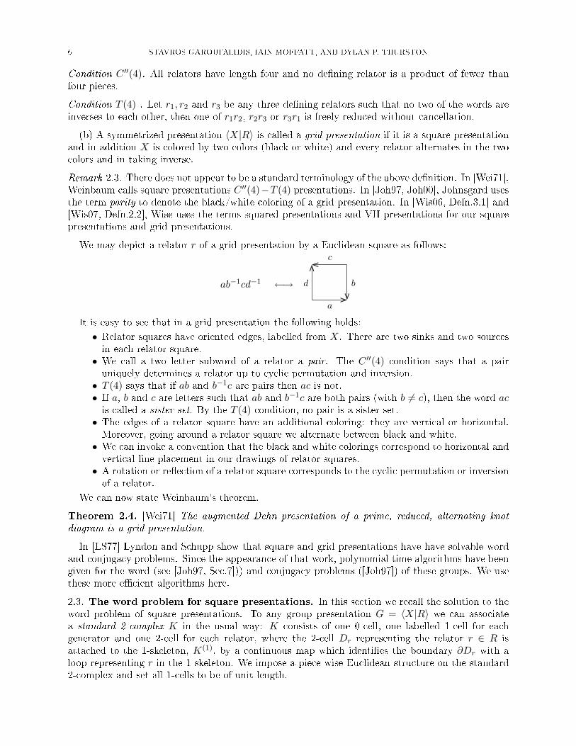
We may depict a relator r of a grid presentation by a Euclidean square as follows:
ab−1cd−1 ←→
c
b
a
d
It is easy to see that in a grid presentation the following holds:
• Relator squares have oriented edges, labelled from X. There are two sinks and two sourcesin each relator square.• We call a two letter subword of a relator a pair. The C ′′(4) condition says that a pairuniquely determines a relator up to cyclic permutation and inversion.• T (4) says that if ab and b−1c are pairs then ac is not.• If a, b and c are letters such that ab and b−1c are both pairs (with b 6= c), then the word acis called a sister-set. By the T (4) condition, no pair is a sister-set.• The edges of a relator square have an additional coloring: they are vertical or horizontal.Moreover, going around a relator square we alternate between black and white.• We can invoke a convention that the black and white colorings correspond to horizontal andvertical line placement in our drawings of relator squares.• A rotation or re�ection of a relator square corresponds to the cyclic permutation or inversionof a relator.
We can now state Weinbaum's theorem.
Theorem 2.4. [Wei71] The augmented Dehn presentation of a prime, reduced, alternating knotdiagram is a grid presentation.
In [LS77] Lyndon and Schupp show that square and grid presentations have have solvable wordand conjugacy problems. Since the appearance of that work, polynomial time algorithms have beengiven for the word (see [Joh97, Sec.7])) and conjugacy problems ([Joh97]) of these groups. We usethese more e�cient algorithms here.
2.3. The word problem for square presentations. In this section we recall the solution to theword problem of square presentations. To any group presentation G = 〈X|R〉 we can associatea standard 2-complex K in the usual way: K consists of one 0-cell, one labelled 1-cell for eachgenerator and one 2-cell for each relator, where the 2-cell Dr representing the relator r ∈ R isattached to the 1-skeleton, K(1), by a continuous map which identi�es the boundary ∂Dr with aloop representing r in the 1-skeleton. We impose a piece-wise Euclidean structure on the standard2-complex and set all 1-cells to be of unit length.
NON-PERIPHERAL IDEAL DECOMPOSITIONS OF ALTERNATING KNOTS 7
A word w represents the identity in G if and only if there is a simply connected planar 2-complex∆, and a map φ : (D, ∂D)→ (K,K(1)) such that the 0-cells are mapped to 0-cells, open i-cells are
mapped to open i-cells, for i = 1, 2 and ∂D is mapped to the loop representing w in K(1). Such a2-complex, labelled in the natural way, is called a Dehn diagram.
Throughout this text we use two concepts of labels of edge-paths of the standard 2-complex,peripheral complex (introduced below) or Dehn diagram. The label of an edge-path is the sequenceof letters determined by the edge-path, where travelling along an edge labelled a contributes theletter a. This is distinct from the word labelling an edge-path, which is the word in the groupdetermined by the path, where travelling along an edge labelled a against the orientation contributesthe letter a−1, and travelling with the orientation, the letter a.
A word in a group presentation is said to be geodesic if it contains the least number of letters overall representatives of the same word, i.e., w is geodesic if |w| = min{|w′| | w =G w′}. A geodesicword represents the identity if and only if it is the empty word. A word in a group presentation isgeodesic if and only if it labels a geodesic edge-path in the standard two complex of the presentation.
A key result of small cancellation theory is the following Geodesic Characterisation Theorem; see[Joh97, Sec.3] and also [Kap97, Lem.3.2].
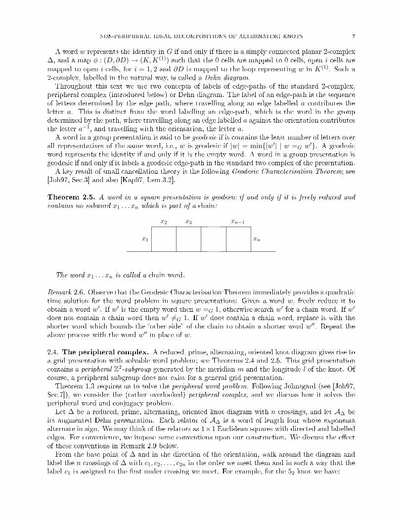
Theorem 2.5. A word in a square presentation is geodesic if and only if it is freely reduced andcontains no subword x1 . . . xn which is part of a chain:
x1
x2 x3 xn−1
xn
The word x1 . . . xn is called a chain word.
Remark 2.6. Observe that the Geodesic Characterisation Theorem immediately provides a quadratictime solution for the word problem in square presentations: Given a word w, freely reduce it toobtain a word w′. If w′ is the empty word then w =G 1, otherwise search w′ for a chain word. If w′
does not contain a chain word then w′ 6=G 1. If w′ does contain a chain word, replace it with theshorter word which bounds the �other side� of the chain to obtain a shorter word w′′. Repeat theabove process with the word w′′ in place of w.
2.4. The peripheral complex. A reduced, prime, alternating, oriented knot diagram gives rise toa grid presentation with solvable word problem; see Theorems 2.4 and 2.5. This grid presentationcontains a peripheral Z2-subgroup generated by the meridian m and the longitude l of the knot. Ofcourse, a peripheral subgroup does not exist for a general grid presentation.
Theorem 1.3 requires us to solve the peripheral word problem. Following Johnsgard (see [Joh97,Sec.7]), we consider the (rather overlooked) peripheral complex, and we discuss how it solves theperipheral word and conjugacy problem.
Let ∆ be a reduced, prime, alternating, oriented knot diagram with n crossings, and let A∆ beits augmented Dehn presentation. Each relator of A∆ is a word of length four whose exponentsalternate in sign. We may think of the relators as 1×1 Euclidean squares with directed and labellededges. For convenience, we impose some conventions upon our construction. We discuss the e�ectof these conventions in Remark 2.9 below.
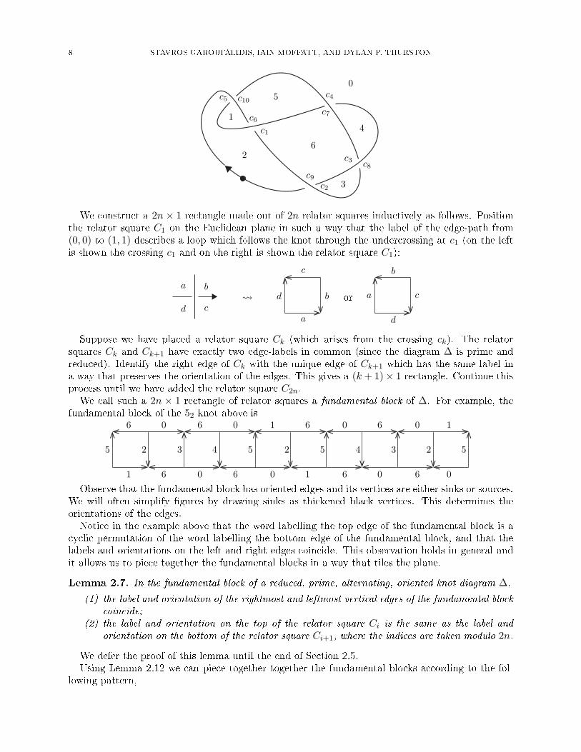
From the base point of ∆ and in the direction of the orientation, walk around the diagram andlabel the n crossings of ∆ with c1, c2, . . . , c2n in the order we meet them and in such a way that thelabel c1 is assigned to the �rst under crossing we meet. For example, for the 52 knot we have:
8 STAVROS GAROUFALIDIS, IAIN MOFFATT, AND DYLAN P. THURSTON
c1
c2
c3
c4c5
c6c7
c8c9
c10
0
1
2
3
4
5
6
We construct a 2n× 1 rectangle made out of 2n relator squares inductively as follows. Positionthe relator square C1 on the Euclidean plane in such a way that the label of the edge-path from(0, 0) to (1, 1) describes a loop which follows the knot through the undercrossing at c1 (on the leftis shown the crossing c1 and on the right is shown the relator square C1):
a b
cd
c
b
a
d or
b
c
d
a
Suppose we have placed a relator square Ck (which arises from the crossing ck). The relatorsquares Ck and Ck+1 have exactly two edge-labels in common (since the diagram ∆ is prime andreduced). Identify the right edge of Ck with the unique edge of Ck+1 which has the same label ina way that preserves the orientation of the edges. This gives a (k + 1)× 1 rectangle. Continue thisprocess until we have added the relator square C2n.
We call such a 2n × 1 rectangle of relator squares a fundamental block of ∆. For example, thefundamental block of the 52 knot above is
6 0 6 0 1 6 0 6 0 1
1 6 0 6 0 1 6 0 6 0
5 2 3 4 5 2 5 4 3 2 5
Observe that the fundamental block has oriented edges and its vertices are either sinks or sources.We will often simplify �gures by drawing sinks as thickened black vertices. This determines theorientations of the edges.
Notice in the example above that the word labelling the top edge of the fundamental block is acyclic permutation of the word labelling the bottom edge of the fundamental block, and that thelabels and orientations on the left and right edges coincide. This observation holds in general andit allows us to piece together the fundamental blocks in a way that tiles the plane.
Lemma 2.7. In the fundamental block of a reduced, prime, alternating, oriented knot diagram ∆,
(1) the label and orientation of the rightmost and leftmost vertical edges of the fundamental blockcoincide;
(2) the label and orientation on the top of the relator square Ci is the same as the label andorientation on the bottom of the relator square Ci+1, where the indices are taken modulo 2n.
We defer the proof of this lemma until the end of Section 2.5.Using Lemma 2.12 we can piece together together the fundamental blocks according to the fol-
lowing pattern,
NON-PERIPHERAL IDEAL DECOMPOSITIONS OF ALTERNATING KNOTS 9
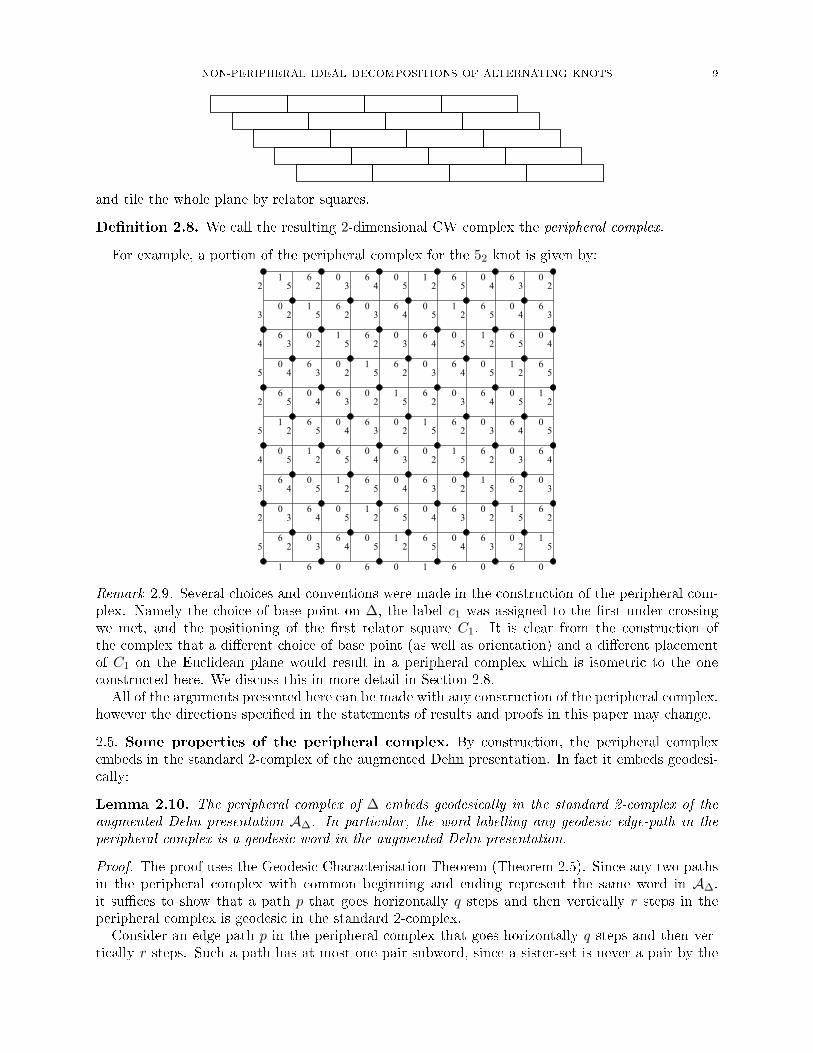
and tile the whole plane by relator squares.
De�nition 2.8. We call the resulting 2-dimensional CW complex the peripheral complex.
For example, a portion of the peripheral complex for the 52 knot is given by:
2
10606
4
1
45253
2
3 4 5 2 5
1 6 0 6 0
3 4 5
0
5 4 3 2
1 6 6 0 1 6 0
2 3 4 5 2 5 4 3
1 6 0 6 0 1 6
2
0
60 0
5 2 3 4 5 2 5 4 3 2 5
2 51 6 0 6 0 1 6 60 0
6
2
1 6 0 6
2 3 4 5
1 6 0
2 3 4
1 6
2 3
1
2
1 6 0 6 0 1
0
3 2 5
0 1 6 60 0
5 2 5 4 3 2 5
6 0 1 6 60 0
4 5 2
4
6 0
3 2 5
60 0
4 3 2 5
6 60 0
5 4 3 2 5
1 6 6 0
2 5
5
0 0
2 3 4 5 2 5 4 3 2 5
1 6 0 6 0 1 6 60
2 3 4 5 2
6
4 3 2 5
0 6 0 1 6 60 0
3 4 5 2 5 4 3 2 5
6 0 6 0 1 6
Remark 2.9. Several choices and conventions were made in the construction of the peripheral com-plex. Namely the choice of base point on ∆, the label c1 was assigned to the �rst under crossingwe met, and the positioning of the �rst relator square C1. It is clear from the construction ofthe complex that a di�erent choice of base point (as well as orientation) and a di�erent placementof C1 on the Euclidean plane would result in a peripheral complex which is isometric to the oneconstructed here. We discuss this in more detail in Section 2.8.
All of the arguments presented here can be made with any construction of the peripheral complex,however the directions speci�ed in the statements of results and proofs in this paper may change.
2.5. Some properties of the peripheral complex. By construction, the peripheral complexembeds in the standard 2-complex of the augmented Dehn presentation. In fact it embeds geodesi-cally:
Lemma 2.10. The peripheral complex of ∆ embeds geodesically in the standard 2-complex of theaugmented Dehn presentation A∆. In particular, the word labelling any geodesic edge-path in theperipheral complex is a geodesic word in the augmented Dehn presentation.
Proof. The proof uses the Geodesic Characterisation Theorem (Theorem 2.5). Since any two pathsin the peripheral complex with common beginning and ending represent the same word in A∆,it su�ces to show that a path p that goes horizontally q steps and then vertically r steps in theperipheral complex is geodesic in the standard 2-complex.
Consider an edge-path p in the peripheral complex that goes horizontally q steps and then ver-tically r steps. Such a path has at most one pair subword, since a sister-set is never a pair by the
10 STAVROS GAROUFALIDIS, IAIN MOFFATT, AND DYLAN P. THURSTON
T (4) condition. Thus we see that the label of the edge-path cannot contain a chain word, as thisrequires two pairs. (Recall the de�nitions of pairs and sister sets from Section 2.2.)
It remains to show that the label of the edge-path is freely reduced. To see why this is we beginby observing that since ∆ is reduced, four distinct regions of ∆ meet at every crossing and thereforeevery relator square has four distinct labels. Now suppose that ab is a subword of the word labellingthe edge-path p. If the subword belongs to the horizontal path, then it labels the bottom of tworelator squares Di and Di+1 in the peripheral complex. By Lemma 2.7, the bottom label of Di+1
is also a label of the top of the relator square Di. This means that b cannot label the bottom of Di
and therefore a 6= b and ab is freely reduced.If the letter a comes from a horizontal edge and b from a vertical edge of p, then the subword ab
labels two sides of a relator square and is therefore freely reduced.Finally, If the subword belongs to the vertical path, then it labels the right hand side of two relator
squares Di and Di+1 in the peripheral complex. By the periodicity of the peripheral complex, theright hand label of Di is also the label of the left hand side of the relator square Di+1. This meansthat b cannot label the right of Di+1 and therefore a 6= b and ab is freely reduced. �
Proof of Lemma 2.7. Since the exponents of the relators of the augmented Dehn presentation alter-nate in sign, all of the orientations of the edges of the fundamental block are of the form requiredby the lemma.
It remains to show that the edge labels are of the required form. First we show that the label onthe top of the relator square Ci is the same as the label on the bottom of the relator square Ci+1
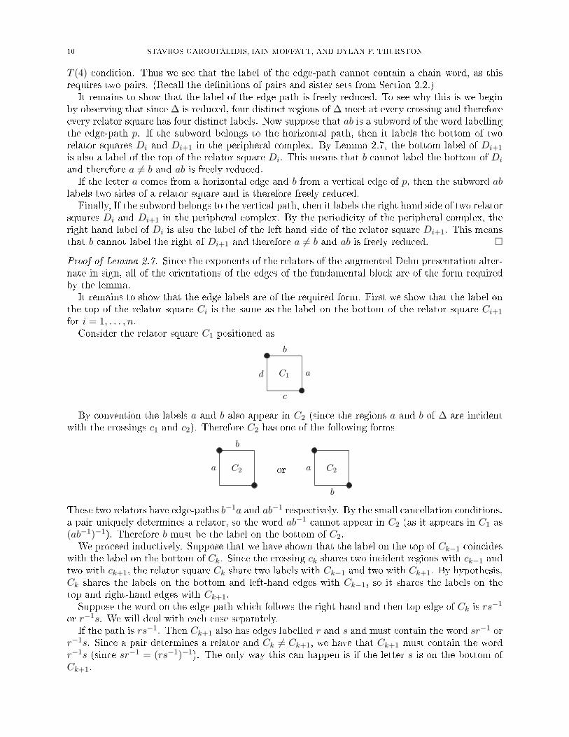
for i = 1, . . . , n.Consider the relator square C1 positioned as
b
a
c
d C1
By convention the labels a and b also appear in C2 (since the regions a and b of ∆ are incidentwith the crossings c1 and c2). Therefore C2 has one of the following forms
b
a C2 or
b
a C2
These two relators have edge-paths b−1a and ab−1 respectively. By the small cancellation conditions,a pair uniquely determines a relator, so the word ab−1 cannot appear in C2 (as it appears in C1 as(ab−1)−1). Therefore b must be the label on the bottom of C2.
We proceed inductively. Suppose that we have shown that the label on the top of Ck−1 coincideswith the label on the bottom of Ck. Since the crossing ck shares two incident regions with ck−1 andtwo with ck+1, the relator square Ck share two labels with Ck−1 and two with Ck+1. By hypothesis,Ck shares the labels on the bottom and left-hand edges with Ck−1, so it shares the labels on thetop and right-hand edges with Ck+1.
Suppose the word on the edge-path which follows the right-hand and then top edge of Ck is rs−1
or r−1s. We will deal with each case separately.If the path is rs−1. Then Ck+1 also has edges labelled r and s and must contain the word sr−1 or
r−1s. Since a pair determines a relator and Ck 6= Ck+1, we have that Ck+1 must contain the wordr−1s (since sr−1 = (rs−1)−1). The only way this can happen is if the letter s is on the bottom ofCk+1.
NON-PERIPHERAL IDEAL DECOMPOSITIONS OF ALTERNATING KNOTS 11
Similarly, if the path is r−1s. Then Ck+1 also has edges labelled r and s and must contain theword s−1r or rs−1. Since a pair determines a relator and Ck 6= Ck+1, we have that Ck+1 mustcontain the word rs−1. The only way this can happen is if the letter s−1 is on the bottom of Ck+1.
We have shown that the label on the top of the relator square Ci is the same as the label on thebottom of the relator square Ci+1 for i = 1, . . . , n.
To complete the proof, consider the relator square C2n in the fundamental block. C2n is of theform
s
r
q
p C2n
where the labels p and q are shared with C2n−1 and r and s are shared with C1 (since c1 and c2n
share incident regions of ∆). But again, the small cancellation conditions say that a pair uniquelydetermines a relator and C2n 6= C1, therefore we must have s = c and r = d, where c and d are thelabels of C1 as shown above. This completes the proof of the lemma. �
Lemma 2.11. In the fundamental block of a reduced, prime, alternating, oriented knot diagram ∆,
(1) the label of an edge-path from the bottom-right to top-left corner of C2n describes a curvehomotopic to a meridional loop, or its inverse, of the knot through the base point of ∆;
(2) the label of an edge-path from the bottom left to top right corner of C2i−1, i = 1, . . . , ndescribes a loop which follows the under-crossing of the knot at c2i−1;
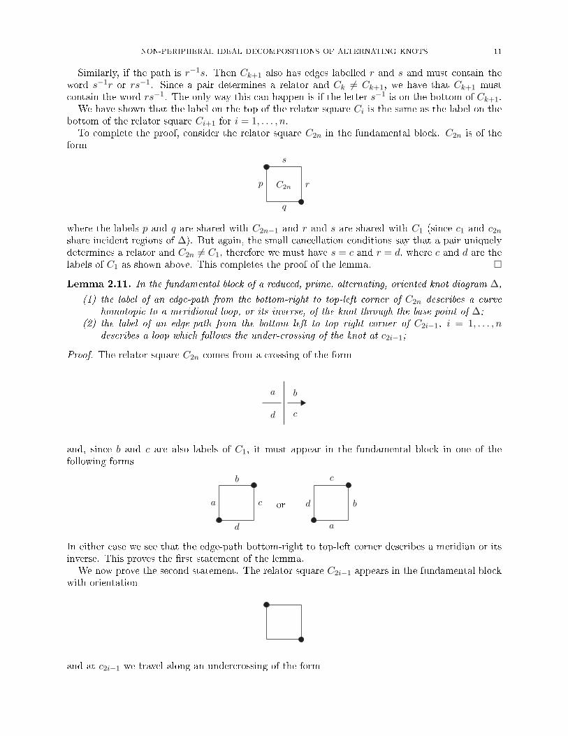
Proof. The relator square C2n comes from a crossing of the form
a b
cd
and, since b and c are also labels of C1, it must appear in the fundamental block in one of thefollowing forms
b
c
d
a or
c
b
a
d
In either case we see that the edge-path bottom-right to top-left corner describes a meridian or itsinverse. This proves the �rst statement of the lemma.
We now prove the second statement. The relator square C2i−1 appears in the fundamental blockwith orientation
and at c2i−1 we travel along an undercrossing of the form
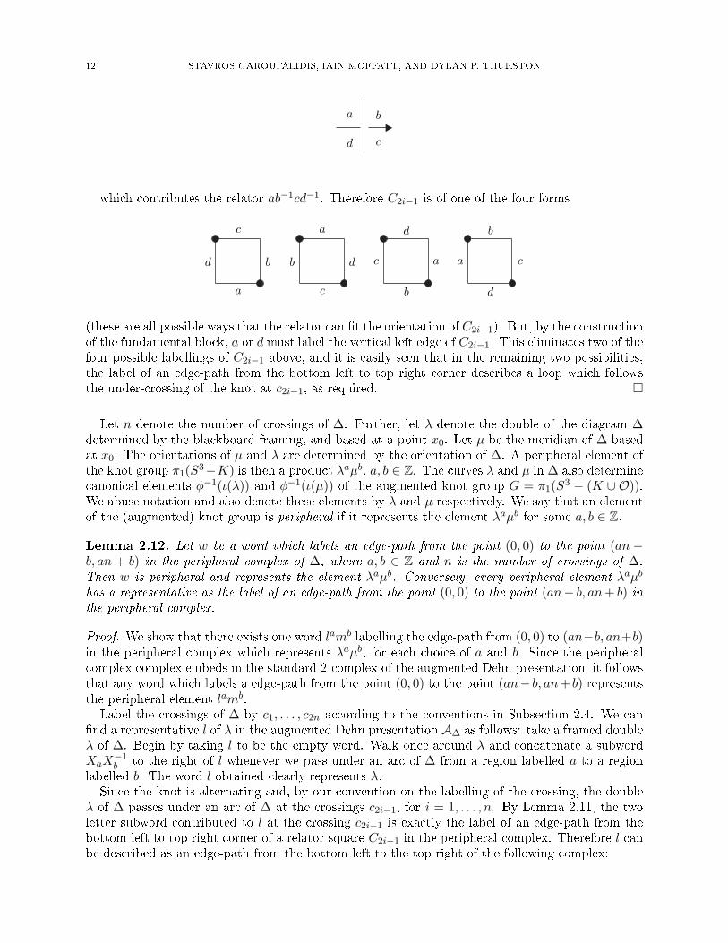
12 STAVROS GAROUFALIDIS, IAIN MOFFATT, AND DYLAN P. THURSTON
a b
cd
which contributes the relator ab−1cd−1. Therefore C2i−1 is of one of the four forms
c
b
a
d
a
d
c
b
d
a
b
c
b
c
d
a
(these are all possible ways that the relator can �t the orientation of C2i−1). But, by the constructionof the fundamental block, a or d must label the vertical left edge of C2i−1. This eliminates two of thefour possible labellings of C2i−1 above, and it is easily seen that in the remaining two possibilities,the label of an edge-path from the bottom left to top right corner describes a loop which followsthe under-crossing of the knot at c2i−1, as required. �
Let n denote the number of crossings of ∆. Further, let λ denote the double of the diagram ∆determined by the blackboard framing, and based at a point x0. Let µ be the meridian of ∆ basedat x0. The orientations of µ and λ are determined by the orientation of ∆. A peripheral element ofthe knot group π1(S3−K) is then a product λaµb, a, b ∈ Z. The curves λ and µ in ∆ also determinecanonical elements φ−1(ι(λ)) and φ−1(ι(µ)) of the augmented knot group G = π1(S3 − (K ∪ O)).We abuse notation and also denote these elements by λ and µ respectively. We say that an elementof the (augmented) knot group is peripheral if it represents the element λaµb for some a, b ∈ Z.
Lemma 2.12. Let w be a word which labels an edge-path from the point (0, 0) to the point (an −b, an + b) in the peripheral complex of ∆, where a, b ∈ Z and n is the number of crossings of ∆.Then w is peripheral and represents the element λaµb. Conversely, every peripheral element λaµb
has a representative as the label of an edge-path from the point (0, 0) to the point (an− b, an+ b) inthe peripheral complex.
Proof. We show that there exists one word lamb labelling the edge-path from (0, 0) to (an−b, an+b)in the peripheral complex which represents λaµb, for each choice of a and b. Since the peripheralcomplex complex embeds in the standard 2-complex of the augmented Dehn presentation, it followsthat any word which labels a edge-path from the point (0, 0) to the point (an− b, an+ b) representsthe peripheral element lamb.
Label the crossings of ∆ by c1, . . . , c2n according to the conventions in Subsection 2.4. We can�nd a representative l of λ in the augmented Dehn presentation A∆ as follows: take a framed doubleλ of ∆. Begin by taking l to be the empty word. Walk once around λ and concatenate a subwordXaX
−1b to the right of l whenever we pass under an arc of ∆ from a region labelled a to a region
labelled b. The word l obtained clearly represents λ.Since the knot is alternating and, by our convention on the labelling of the crossing, the double
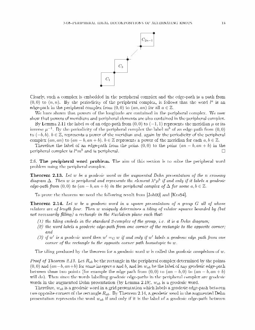
λ of ∆ passes under an arc of ∆ at the crossings c2i−1, for i = 1, . . . , n. By Lemma 2.11, the twoletter subword contributed to l at the crossing c2i−1 is exactly the label of an edge-path from thebottom left to top right corner of a relator square C2i−1 in the peripheral complex. Therefore l canbe described as an edge-path from the bottom left to the top right of the following complex:
NON-PERIPHERAL IDEAL DECOMPOSITIONS OF ALTERNATING KNOTS 13
C1
C3
C2n−1
Clearly, such a complex is embedded in the peripheral complex and the edge-path is a path from(0, 0) to (n, n). By the periodicity of the peripheral complex, it follows that the word la is anedge-path in the peripheral complex from (0, 0) to (an, an) for all a ∈ Z.
We have shown that powers of the longitude are contained in the peripheral complex. We nowshow that powers of meridians and peripheral elements are also contained in the peripheral complex.
By Lemma 2.11 the label m of an edge-path from (0, 0) to (−1, 1) represents the meridian µ or itsinverse µ−1. By the periodicity of the peripheral complex the label mb of an edge path from (0, 0)to (−b, b), b ∈ Z, represents a power of the meridian and, again by the periodicity of the peripheralcomplex (an, an) to (an− b, an+ b), b ∈ Z represents a power of the meridian for each a, b ∈ Z.
Therefore the label of an edge-path from the point (0, 0) to the point (an − b, an + b) in theperipheral complex is lamb and is peripheral. �
2.6. The peripheral word problem. The aim of this section is to solve the peripheral wordproblem using the peripheral complex.
Theorem 2.13. Let w be a geodesic word in the augmented Dehn presentation of the n crossingdiagram ∆. Then w is peripheral and represents the element λaµb if and only if it labels a geodesicedge-path from (0, 0) to (an− b, an+ b) in the peripheral complex of ∆ for some a, b ∈ Z.
To prove the theorem we need the following result from [Joh00] and [Kra94].
Theorem 2.14. Let w be a geodesic word in a square presentation of a group G all of whoserelators are of length four. Then w uniquely determines a tiling of relator squares bounded by (butnot necessarily �lling) a rectangle in the Euclidean plane such that:
(1) the tiling embeds in the standard 2-complex of the group, i.e. it is a Dehn diagram;(2) the word labels a geodesic edge-path from one corner of the rectangle to the opposite corner;
and(3) if w′ is a geodesic word then w′ =G w if and only if w′ labels a geodesic edge-path from one
corner of the rectangle to the opposite corner path homotopic to w.
The tiling produced by the theorem for a geodesic word w is called the geodesic completion of w.
Proof of Theorem 2.13. Let Rab be the rectangle in the peripheral complex determined by the points(0, 0) and (an−b, an+b) for some integers a and b, and let wab be the label of any geodesic edge-pathbetween these two points (for example the edge-path from (0, 0) to (an − b, 0) to (an − b, an + b)will do). Then since the words labelling geodesic edge-paths in the peripheral complex are geodesicwords in the augmented Dehn presentation (by Lemma 2.10), wab is a geodesic word.
Therefore, wab is a geodesic word in a grid presentation which labels a geodesic edge-path betweentwo opposite corners of the rectangle Rab. By Theorem 2.14, a geodesic word in the augmented Dehnpresentation represents the word wab if and only if it is the label of a geodesic edge-path between

14 STAVROS GAROUFALIDIS, IAIN MOFFATT, AND DYLAN P. THURSTON
(0, 0) and (an− b, an+ b). So all geodesic representatives of wab are words labelling geodesic edge-paths from (0, 0) and (an − b, an + b) in the peripheral complex. Finally, by Lemma 2.12, everyperipheral element is presented by a word wab for some a, b ∈ Z and the result follows. �
2.7. Proof of Theorem 1.3. Let ∆ be a prime, reduced alternating projection of a knot K in S3.Theorem 1.3 follows from the following lemma.
Lemma 2.15. (a) The Wirtinger arcs, Wirtinger loops, and Dehn arcs and conjugates of the shortarcs of ∆ have explicit geodesic representatives in the peripheral complex.(b) The above geodesic representatives of Wirtinger arcs, Wirtinger loops and Dehn arcs are non-peripheral, and the above geodesic representatives of the short arcs are not conjugate to a peripheralelement.
Proof. We apply the notation and discussion from the last three paragraphs of Subsection 2.1.Let w be a word representing a Wirtinger arc, Wirtinger loop, short arc or Dehn arc of ∆. Recall
the map φ from Equation (2) and the method for reading the a representative word φ−1(ι(w)) inthe augmented Dehn presentation described in Remark 2.1. We use the peripheral complex to showthat its image φ−1(ι(w)) is non-peripheral.
We deal with each type of loop separately. Throughout we let l = l1l2 · · · l2n be a geodesicrepresentative of λ which was constructed in the proof of Lemma 2.12. It is given by an edge-pathfollowing the sequence of relator squares C1, C2, . . . , C2n−1. Each two letter subword l2i−1l2i of llabels an edge path on C2i−1. Also letm = m1m2 be a geodesic representative of µ in the augmentedDehn presentation. By Theorem 2.13, l and m are labels of edge paths from (0, 0) to (n, n) and(0, 0) to (−1, 1) respectively, in the peripheral complex.Wirtinger arcs: Wirtinger arcs are loops which follow the double λ of ∆ returning to the base-point after passing through fewer than 2n crossings. Therefore a Wirtinger loop is represented by asubword l1l2 · · · l2p, wher 2p < 2n, of l. Moreover, l1l2 · · · l2p is represented by the label of any edge-path from (0, 0) to (p, p) for p < n. By Theorem 2.13, it follows that l1l2 · · · l2p is non-peripheral asit does not label a path between (0, 0) and (an− b, an+ b).Wirtinger loops: We may move a Wirtinger loop close to some crossing ci. By the way that therelators of the augmented Dehn presentation are read from ∆ (see Subsection 2.1), we see that theWirtinger loop can be described by a geodesic edge-path between two opposite corners of Di (whichtwo opposite corners depends on the given Wirtinger loop). Let the label of this edge-path be w.
The word w is geodesic of length two. Therefore, if w is peripheral it must represent µ±1.However, by Lemma 2.11, the only geodesic words which represent µ±1 arise as a path from (0, 0)to (∓1,±1) in the peripheral complex, so w cannot be the label of such an edge-path since by thede�nition of Wirtinger loops, w is not a representative of the meridian, which is described by a pathfrom (0, 0) and (−1, 1).Dehn arcs: Suppose that a given Dehn arc intersects the bounded region a of ∆. Then it isrepresented by XaX
−10 in the augmented Dehn presentation. The word XaX
−10 is geodesic since it
is freely reduced (a 6= 0) and clearly does not contain a chain subword (see Theorem 2.5).The meridian µ has exactly two geodesic representatives which label the edge-path (0, 0) to (−1, 1)
of C2n. It is easily seen from the de�nition of Dehn arcs that neither of these words can be XaX−10 .
Short arcs: Short arcs are found by walking around the double λ of ∆, and at some point, jumpingto an adjacent arc of λ and walking back to the base point in one of two ways. Short arcs are thenrepresented by words of the form
(3) l1l2 · · · lklp · · · l2n
and
(4) l1l2 · · · lklp · · · l1.
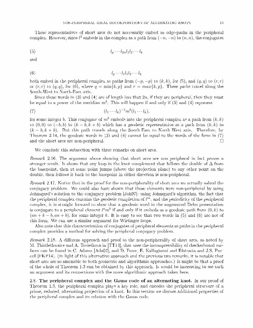
NON-PERIPHERAL IDEAL DECOMPOSITIONS OF ALTERNATING KNOTS 15
These representatives of short arcs do not necessarily embed as edge-paths in the peripheralcomplex. However, since l2 embeds in the complex as a path from (−n,−n) to (n, n), the conjugates
(5) lp · · · l2nl1l2 · · · lkand
(6) lp · · · l1l1l2 · · · lkboth embed in the peripheral complex as paths from (−p,−p) to (k, k), for (5), and (q, q) to (r, r)or (r, r) to (q, q), for (6), where q = min{k, p} and r = max{k, p}. These paths travel along theSouth-West to North-East axis.
Since these words in (3) and (4) are of length less that 2n, if they are peripheral, then they mustbe equal to a power of the meridian mb. This will happen if and only if (3) and (4) represent
(7) (l1 · · · lk)−1mb(l1 · · · lk),
for some integer b. This conjugate of mb embeds into the peripheral complex as a path from (k, k)to (0, 0) to (−b, b) to (k − b, k + b) which has a geodesic representative as a path from (k, k) to(k − b, k + b). But this path travels along the South-East to North-West axis. Therefore, byTheorem 2.14, the geodesic words in (3) and (4) cannot be equal to the words of the form in (7)and the short arcs are non-peripheral. �
We conclude this subsection with three remarks on short arcs.
Remark 2.16. The argument above showing that short arcs are non-peripheral in fact proves astronger result. It shows that any loop in the knot complement that follows the double of ∆ fromthe basepoint, then at some point jumps (above the projection plane) to any other point on thedouble, then follows it back to the basepoint in either direction is non-peripheral.
Remark 2.17. Notice that in the proof for the non-peripherality of short arcs we actually solved theconjugacy problem. We could also have shown that these elements were non-peripheral by usingJohnsgard's solution to the conjugacy problem [Joh97]: using Johnsgard's algorithm, the fact thatthe peripheral complex contains the geodesic completion of lm, and the periodicity of the peripheralcomplex, it is straight-forward to show that a geodesic word in the augmented Dehn presentationis conjugate to a peripheral element lamb if and only if it embeds as a geodesic path from (0, k) to(an + k − b, an + b), for some integer k. It is easy to see that two words in (5) and (6) are not ofthis form. We can use a similar argument for Wirtinger loops.
Also note that this characterisation of conjugates of peripheral elements as paths in the peripheralcomplex provides a method for solving the peripheral conjugacy problem.
Remark 2.18. A di�erent approach and proof to the non-peripherality of short arcs, as noted byM. Thistlethwaite and A. Tsvietkova in [TT14], that uses the incompressibility of checkerboard sur-faces can be found in C. Adams [Ada07], and D. Futer, E. Kalfagianni and Efstratia and J.S. Pur-cell [FKP14]. (In light of this alternative approach and the previous two remarks, it is notable thatshort arcs are so amenable to both geometric and algorithmic approaches.) It might be that a proofof the whole of Theorem 1.3 can be obtained by this approach. It would be interesting to see suchan argument and its connections with the more algorithmic approach taken here.
2.8. The peripheral complex and the Gauss code of an alternating knot. In our proof ofTheorem 1.3, the peripheral complex plays a key role, and encodes the peripheral structure of aprime, reduced, alternating projection of a knot. In this section we discuss additional properties ofthe peripheral complex and its relation with the Gauss code.
16 STAVROS GAROUFALIDIS, IAIN MOFFATT, AND DYLAN P. THURSTON
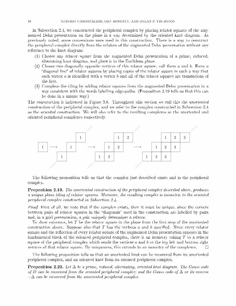
In Subsection 2.4, we constructed the peripheral complex by placing relator squares of the aug-mented Dehn presentation on the plane in a way determined by the oriented knot diagram. Aspreviously noted, some conventions were used in this construction. There is a way to constructthe peripheral complex directly from the relators of the augmented Dehn presentation without anyreference to the knot diagram:
(1) Choose any relator square from the augmented Dehn presentation of a prime, reduced,alternating knot diagram, and place it in the Euclidean plane.
(2) Choose two diagonally opposite vertices of this relator square, call them a and b. Form a�diagonal line� of relator squares by placing copies of the relator square in such a way thateach vertex a is identi�ed with a vertex b and all of the relator squares are translations ofthe �rst.
(3) Complete the tiling by adding relator squares from the augmented Dehn presentation in away consistent with the words labelling edge-paths. (Proposition 2.19 tells us that this canbe done in a unique way.)
The construction is indicated in Figure 2.8. Throughout this section we call this the unorientedconstruction of the peripheral complex, and we refer to the complex constructed in Subsection 2.4as the oriented construction. We will also refer to the resulting complexes as the unoriented andoriented peripheral complexes respectively.
1
1
1
1
1
1
1
2
2
2
1
1
1
3
3
3
2
2
2
The following proposition tells us that the complex just described exists and is the peripheralcomplex.
Proposition 2.19. The unoriented construction of the peripheral complex described above, producesa unique plane tiling of relator squares. Moreover, the resulting complex is isometric to the orientedperipheral complex constructed in Subsection 2.4.
Proof. First of all, we note that if the complex exists, then it must be unique, since the cornersbetween pairs of relator squares in the �diagonals� used in the construction are labelled by pairsand, in a grid presentation, a pair uniquely determines a relator.
To show existence, let T be the relator square in the plane from the �rst step of the unorientedconstruction above. Suppose also that T has the vertices a and b speci�ed. Since every relatorsquare and the re�ection of every relator square of the augmented Dehn presentation appears in thefundamental block of the oriented peripheral complex, there is an isometry taking T to a relatorsquare of the peripheral complex which sends the vertices a and b to the top-left and bottom-rightvertices of that relator square. By uniqueness, this extends to an isometry of the complexes. �
The following proposition tells us that an unoriented knot can be recovered from its unorientedperipheral complex, and an oriented knot from its oriented peripheral complex.
Proposition 2.20. Let ∆ be a prime, reduced, alternating, oriented knot diagram. The Gauss codeof D can be recovered from the oriented peripheral complex; and the Gauss code of ∆ or its inverse−∆ can be recovered from the unoriented peripheral complex.
NON-PERIPHERAL IDEAL DECOMPOSITIONS OF ALTERNATING KNOTS 17
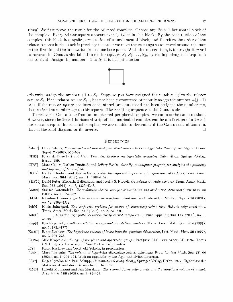
Proof. We �rst prove the result for the oriented complex. Choose any 2n × 1 horizontal block ofthe complex. Every relator square appears exactly twice in this block. By the construction of thecomplex, this block is a cyclic permutation of a fundamental block, and therefore the order of therelator squares in the block is precisely the order we meet the crossings as we travel around the knotin the direction of the orientation from some base point. With this observation, it is straight-forwardto recover the Gauss code: label the relator squares S1, S2, . . . , S2n by reading along the strip fromleft to right. Assign the number −1 to S1 if it has orientation
otherwise assign the number +1 to S1. Suppose you have assigned the number ±j to the relatorsquare Si. If the relator square Si+1 has not been encountered previously assign the number ∓(j+1)to it, if the relator square has been encountered previously and has been assigned the number ±p,then assign the number ∓p to this square. The resulting sequence is the Gauss code.
To recover a Gauss code from an unoriented peripheral complex, we can use the same method.However, since the 2n× 1 horizontal strip of the unoriented complex can be a re�ection of a 2n× 1horizontal strip of the oriented complex, we are unable to determine if the Gauss code obtained isthat of the knot diagram or its inverse. �
References
[Ada07] Colin Adams, Noncompact Fuchsian and quasi-Fuchsian surfaces in hyperbolic 3-manifolds, Algebr. Geom.Topol. 7 (2007), 565�582.
[BP92] Riccardo Benedetti and Carlo Petronio, Lectures on hyperbolic geometry, Universitext, Springer-Verlag,Berlin, 1992.
[CDW] Marc Culler, Nathan Dun�eld, and Je�ery Weeks, SnapPy, a computer program for studying the geometry
and topology of 3-manifolds.[DG12] Nathan Dun�eld and Stavros Garoufalidis, Incompressibility criteria for spun-normal surfaces, Trans. Amer.
Math. Soc. 364 (2012), no. 11, 6109�6137.[FKP14] David Futer, Efstratia Kalfagianni, and Jessica S. Purcell, Quasifuchsian state surfaces, Trans. Amer. Math.
Soc. 366 (2014), no. 8, 4323�4343.[Gar08] Stavros Garoufalidis, Chern-Simons theory, analytic continuation and arithmetic, Acta Math. Vietnam. 33
(2008), no. 3, 335�362.[Hik01] Kazuhiro Hikami, Hyperbolic structure arising from a knot invariant, Internat. J. Modern Phys. A 16 (2001),
no. 19, 3309�3333.[Joh97] Karin Johnsgard, The conjugacy problem for groups of alternating prime tame links is polynomial-time,
Trans. Amer. Math. Soc. 349 (1997), no. 3, 857�901.[Joh00] , Geodesic edge paths in nonpositively curved complexes, J. Pure Appl. Algebra 147 (2000), no. 1,
59�93.[Kap97] Ilya Kapovich, Small cancellation groups and translation numbers, Trans. Amer. Math. Soc. 349 (1997),
no. 5, 1851�1875.[Kas97] Rinat Kashaev, The hyperbolic volume of knots from the quantum dilogarithm, Lett. Math. Phys. 39 (1997),
no. 3, 269�275.[Kra94] Mile Krajcevski, Tilings of the plane and hyperbolic groups, ProQuest LLC, Ann Arbor, MI, 1994, Thesis
(Ph.D.)�State University of New York at Binghamton.[KY] Rinat Kashaev and Yoshiyuki Yokota, in preparation.[Lac04] Marc Lackenby, The volume of hyperbolic alternating link complements, Proc. London Math. Soc. (3) 88
(2004), no. 1, 204�224, With an appendix by Ian Agol and Dylan Thurston.[LS77] Roger Lyndon and Paul Schupp, Combinatorial group theory, Springer-Verlag, Berlin, 1977, Ergebnisse der
Mathematik und ihrer Grenzgebiete, Band 89.[MM01] Hitoshi Murakami and Jun Murakami, The colored Jones polynomials and the simplicial volume of a knot,
Acta Math. 186 (2001), no. 1, 85�104.
18 STAVROS GAROUFALIDIS, IAIN MOFFATT, AND DYLAN P. THURSTON
[NZ85] Walter Neumann and Don Zagier, Volumes of hyperbolic three-manifolds, Topology 24 (1985), no. 3, 307�332.
[Oht17] Tomotada Ohtsuki, On the asymptotic expansion of the Kashaev invariant of the 52-knot, Quantum Topol.(2017).
[OY16] Tomotada Ohtsuki and Yoshiyuki Yokota, On the asymptotic expansions of the Kashaev invariant of the
knots with 6 crossings, 2016, Preprint.[SY] Makoto Sakuma and Yoshiyuki Yokota, An application of non-positively curved cubings of alternating links,
In preparation.[Thu77] William Thurston, The geometry and topology of 3-manifolds, Universitext, Springer-Verlag, Berlin, 1977,
Lecture notes, Princeton.[Thu99] Dylan Thurston, Hyperbolic volume and the Jones polynomial, Notes from lectures at the Grenoble summer
school �Invariants des n÷uds et de variétés de dimension 3�, June 1999, available from http://pages.iu.
edu/~dpthurst/speaking/Grenoble.pdf.[Til12] Stephan Tillmann, Degenerations of ideal hyperbolic triangulations, Math. Z. 272 (2012), no. 3-4, 793�823.[TT14] Morwen Thistlethwaite and Anastasiia Tsvietkova, An alternative approach to hyperbolic structures on link
complements, Algebr. Geom. Topol. 14 (2014), no. 3, 1307�1337.[Wee05] Je� Weeks, Computation of hyperbolic structures in knot theory, Handbook of knot theory, Elsevier B. V.,
Amsterdam, 2005, pp. 461�480.[Wei71] Carl Weinbaum, The word and conjugacy problems for the knot group of any tame, prime, alternating knot,
Proc. Amer. Math. Soc. 30 (1971), 22�26.[Wis06] Daniel Wise, Subgroup separability of the �gure 8 knot group, Topology 45 (2006), no. 3, 421�463.[Wis07] , Complete square complexes, Comment. Math. Helv. 82 (2007), no. 4, 683�724.[Yok02] Yoshiyuki Yokota, On the potential functions for the hyperbolic structures of a knot complement, Invariants
of knots and 3-manifolds (Kyoto, 2001), Geom. Topol. Monogr., vol. 4, Geom. Topol. Publ., Coventry, 2002,pp. 303�311 (electronic).
[Yok11] , On the complex volume of hyperbolic knots, J. Knot Theory Rami�cations 20 (2011), no. 7, 955�976.
School of Mathematics, Georgia Institute of Technology, Atlanta, GA 30332-0160, USA
http://www.math.gatech.edu/~stavros
E-mail address: [email protected]
Department of Mathematics, Royal Holloway, University of London, Egham, Surrey, TW20 0EX,
United Kingdom
http://www.personal.rhul.ac.uk/uxah/001
E-mail address: [email protected]
Department of Mathematics, Indiana University, Bloomington, IN 47405-7106, USA
http://pages.iu.edu/~dpthurst
E-mail address: [email protected]