1

Non-Tariff Measures Trickling through Global Value Chains

Mahdi Ghodsi and Robert Stehrer

The Vienna Institute for International Economic Studies (wiiw)

Rahlgasse 3, 1060 Vienna, Austria

www.wiiw.ac.at.

Draft version: 19/05/2016

Abstract

In the current globalization process geographical and local production processes are intertwined

through global value chains (GVC). In the presence of GVCs import tariffs therefore do not only

affect the direct trading partners but also have indirect impact through international industrial

linkages. This is also the case for non-tariff measures (NTMs) which have gained importance in the

last decades. The paper analyses these indirect effects of these trade policy instruments in the global

economy. In a four-stage approach, the cumulative impacts of trade policy measures along GVCs

using the world input-output database (WIOD) are quantified. In the first stage, bilateral import

demand elasticities consistent with WIOD classification are estimated. In the second stage, bilateral

ad-valorem equivalents (AVE) of nine types of NTMs notified to the WTO by the end of 2011 are

quantified. Then, cumulative bilateral-trade restrictiveness indices (BRIs) using the AVEs of NTMs

and tariffs taking into account backward linkages are calculated. Finally, in the fourth step the impact

of trade policy measures on the average annual growth of labour productivity is assessed.

Summarising, the paper offers detailed BRIs for the inputs of 35 WIOD industries to 41 economies

from 2002 to 2011, thus providing insights on the path of NTMs to the downstream industries and the

final absorption.

Keywords: non-tariff measures, global value chains, cumulative ad-valorem equivalents, labour

productivity

JEL codes: F13, F14

This paper was produced as part of the project "Productivity, Non-Tariff Measures and Openness" (PRONTO) funded by the

European Commission under the 7th Framework Programme, Theme SSH.2013.4.3-3 "Untapped Potential for Growth and

Employment Reducing the Cost of Non-Tariff Measures in Goods, Services and Investment", Grant agreement No. 613504.

2

1 Introduction

There are certain legitimate motives for the imposition of non-tariff measures (NTMs). When a

foreign imported product potentially harms the domestic consumers’ health, safety, animal health,

environmental quality, etc. countries are allowed to restrict the importation of these products. Specific

standards are regulated within qualitative NTMs such as sanitary and phytosanitary measures (SPS),

and technical barriers to trade (TBTs) to assure certain standards and characteristics of imported

products. Such regulations affect trade flows and prices of products at different stages of production

in various ways. For instance, chemicals used in the first stages of production can be the focus of a

prohibitive TBT, which can influence the cost of production for downstream products where this

product is used as intermediary. In contrast, some market efficiency regulations such as mandatory

labelling set within TBTs can improve the transparent information to the consumers and producers

who can utilize the intermediates to their production with lower transaction costs.

The ability of the exporters to comply with the NTMs is diverse across countries. It might be the case

that certain countries which are already producing in line with the imposed regulations are not harmed

or even can increase their exports (due to re-direction effects or a general increase in demand due to

quality improvements caused by the NTM). In contrast, some other countries’ exports that are not in

line with the measures in the destination market might be restricted. The consequence of a specific

qualitative NTM might even result in absolute prohibition until the product complies with the

implemented standards. Domestic producers in need of intermediate inputs from abroad then alter

their demand to those import sources who comply with the new regulations. Therefore, responses of

the domestic producers to the NTMs affecting their inputs are heterogeneous across sourcing

countries depending on the exporters’ capabilities to cope with the standards.

Quantitative NTMs, such as safeguards (SG), special safeguards (SSG), countervailing measures

(CV), anti-dumping (ADP), and quantitative restrictions (QR) are usually imposed against restrictive

or discriminative policy measures imposed by the trade partners. While the motivations behind these

NTMs are not purely qualitative issues, these measures might also have some quality impact on the

imported product (see Ghodsi, Jokubauskaite and Stehrer, 2015). Besides, such implemented measure

might – similar to qualitative NTMs - lead to a trade creation effect. Moreover, unlike TBTs,

quantitative NTMs are usually imposed bilaterally against a specific trade partner on a certain product

which might lead to a trade diversion effect increasing the import from a third country. Therefore, the

impact of the aforementioned quantitative NTMs might again be diverse across trading partners and

products.

In addition to these seven types of NTMs, countries can raise specific trade concerns (STCs) on the

TBT and/or SPS imposed by other WTO members. These STCs are raised mainly due to the trade

restrictiveness of special cases of TBT or SPS. Some parts of these STCs are already notified by the

3

imposing country to the WTO notifications. However, some STCs are not directly notified by the

maintaining member. It is argued that governments sometimes are reluctant to notify their

implemented NTMs to avoid trade conflicts, which reduces the transparency of trade policies.

Therefore, WTO established TBT and SPS committees to allow member states to discuss the policy

measures imposed by other countries. These STCs have certain impact on bilateral trade flows, which

sometimes lead to Dispute Settlement cases within the WTO (Ghodsi and Michalek, 2014).

Firms and industries are affected by (trade policy) measures through three channels. The first channel

can be identified as a protectionist measure imposed against the competitors of an industry within the

domestic market which is imposed by the domestic government. The second channel can refer to

measures levied against the inputs of production of an industry, which usually imposes extra costs on

the intermediate inputs of production in previous stages of production. The third channel comprises

those measures that the industry faces while exporting to the foreign destinations. Depending on the

type of measures implemented within each channel industries are affected differently.

Considering global value chains (GVCs) one can track NTMs’ traces on the second channel of trade

policy (TP) using measures of backward and forward linkages. Diverse impacts of various types of

NTMs need to be carefully taken into consideration while studying their role in GVCs. Usually, tariffs

and NTMs levied on the first-stage inputs of production exhibit a direct impact on the cost of

production. However, heterogeneous effects of NTMs at previous stages of production might impact

on costs and trade patterns of downstream sectors.

Therefore, the paper aims at studying such measures and the way they trickle through GVCs by

assessing their role in sectoral performance across forty economies in the world. The main goal of this

paper is to study the direct and indirect effects of NTMs through backward and forward linkages

within GVCs, and assess their role in the growth of labour productivity of services and non-services

sectors.

In order to achieve this goal, the methodological approach is divided in to four stages. In the first

stage, the bilateral import demand elasticities are estimated as the first major contribution in the

literature. At the second stage, the bilateral impacts of nine types of NTMs on the import flows are

assessed by calculating ad-valorem equivalents (AVE) of the NTMs using the above elasticities as

another major contribution within the literature. The third stage provides the calculation of bilateral-

trade restrictiveness indices (BRIs) that are levied against the upstream sectors of production for each

sector. The fourth stage then analyses the impact of three channels of such measures on the labour

productivity growth during the period.

The rest of the paper is organized as follows. In the next section we shortly overview the literature on

the topic. The third section discusses the four stages of methodological approach and the data applied

in the analysis. The fourth section presents the findings and, finally, section five concludes.

4

2 Literature

There exist a large number of recent studies acknowledging the opaque nature of NTMs. Complexity

of the NTMs is argued by the diversity of the motives of the governments in addition to their various

consequences. Substitutability for tariffs (Moore and Zanardi, 2011; Ghodsi, 2015a), substitutability

for other NTMs (Rosendorff, 1996), and policy retaliation (Vandenbussche and Zanardi, 2008; de

Almeida et al., 2012; Sanjuán López et al., 2013) are political motives behind the imposition of NTMs

that might lead to trade disturbances and prohibitions. In contrast, safety, health, and environmental

issues (Otsuki et al., 2001; Ghodsi, 2015a) and technological advancement and innovation are the

qualitative issues that might have short term hampering impact on trade but a positive long run effect

due to positive externalities (Beghin et al., 2012). The various causes of NTMs left no solid consensus

for the general impact of each type of NTM among scholars. Hence, it might be more appropriate to

analyse the causes and effects of each measure separately instead of giving a general conclusion

regarding the diverse effect of NTMs given their ambiguity and complexity.

The estimation of the ad-valorem equivalent (AVE) for NTMs was proposed by Kee et al. (2009)

using cross sectional trade data at the 6-digit level of the Harmonized System (HS) for 2002. They

constrained their results to only the positive AVEs pointing at hampering effect on trade. This

approach was then applied by Beghin et al. (2014) and Bratt (2014), however allowing for negative

AVEs representing promotive behaviour of the NTM. In these studies, all types of NTMs were

included as a dummy variable indicating whether any type of NTM was in force on the bilateral trade

flow. Moreover, the estimates at the product level provided only one estimator of the impact of NTMs

across all countries. The unilateral elasticites used in those studies were borrowed from Kee et al.

(2008), which by construction vary across countries only through variations of import-GDP share of

the given product across countries. Hence, in those studies, the variation of the AVE of all NTMs for

a single product across countries only comes from the variation of import-GDP share. The

shortcoming of those approaches is that the impact of the imposed NTMs by various countries on a

single product is assumed to be uniform and is captured by a single estimator. Ghodsi, Grübler, and

Stehrer (2015) extend the approach to have the NTMs impact varying by the importing countries

using bilateral trade flows. In this study, we extend that empirical strategy differentiating the impact

of NTMs by types, by products, by the imposing country, and by the exporting country facing them.

The concept of global value chains (GVC) stems from the first concepts of classical economics’

theory of value by Piero Sraffa on his book titled ‘Production of commodities by means of

commodities’ (Sraffa, 1975). During 1980s in a research proposal on the modern world system,

Hopkins and Wallerstein (1977) elaborated the concept of commodity chains in a macro and holistic

perspective as whatsoever inputs that a final consumable good needs to reach the final consumer. The

process in which any types of raw materials, services, transportation mechanisms, etc., or even a food

inputs into the labour at any stages of production of all those inputs used for an ultimate consumable

5

item was termed as commodity chains. Later on, Gereffi (1994) established a study framework on

global commodity chains (GCC) in a meso or micro perspective. Industrial organization and structural

governance in the economic literature of international business discussed in various studies such as

Porter (1985) shifted the concept towards the GVC, which is not conceptually far from GCC. Studies

such as Gereffi et al. (2005), and Gereffi and Sturgeon (2013) however, use GVC in explaining the

industrial characteristics and performances through inter-firm and inter-industry relations.1

Trade liberalization, decreasing tariffs, and other trade barriers by international and multilateral

agreements lead to a dominant role of GVC in the world economy. Moreover, existing offshoring

strategies, outsourcing of activities and global fragmentation of production of goods and services are

emerging due to the reduced transaction costs by technological development in recent decades, such

as the improvement in the information and telecommunication (ICT) services. In fact, ICT services

advancement replaced the traditional transport costs, which are also parts of the GVC as major

services sectors (Backer and Miroudot, 2013).

The importance of GVC was emphasized more compiling the World Input-Output Databases (WIOD)

by Timmer et al. (2012). Many scholars have proposed and used frameworks to track the GVC

through WIOD. Antràs et al. (2012) establishes a framework to calculate upstreamness of sectors as

the stages of production within GVC to the ultimate consumable item. Using the same methodology

and considering the whole world as a single economy, Hagemejer and Ghodsi (2014) find that

upstreamness within the European Union (EU) New Member States (NMS) has increased due to

liberalization in trade with the old member states. Backer and Miroudot (2013) also show that number

of stages within the GVC has increased during 1995-2008, which indicates a dominant role of trade

liberalization in global fragmentation of production. This implicates that services and manufacturing

are more intertwined, and their shares of value-added in each other’s value added is becoming more

dominant in the globalization process (OECD, 2013).

The intertwined sectors within GVC can be referred more as a network of industries, in which a

simple shock in one reflects as a butterfly effect along GVC. Considering tariffs as a policy shock to a

specific sector, all users of that sector are affected along the GVC. Rouzet and Miroudot (2013)

proposed a framework to calculate the cumulative effect of such a shock. In fact, their approach

calculates the cumulative costs of tariffs against the inputs of a given sector. Miroudot et al. (2013)

use the same methodology to estimate the cumulative tariffs on the inputs of services sectors. In fact,

they track the effects of tariffs against non-services industries on the production and exports of

services and find a downward trend of cumulative tariffs on services sectors for majority of countries

from 2000 to 2009 due to liberalization through WTO commitments.

The relationship between productivity growth and trade openness is also widely studied in the

literature (e.g. Harrison, 1996; Edwards, 1998; Frankel and Romer, 1999; Rodriguez and Rodrik,

1 For further study on the conceptual evolution of GVC, see Bair (2005).

6

2001). Grossman and Helpman (1993) argue that diffusion of knowledge through the inputs of

production traded to a country increases the innovative capacities and consequently productivity. Coe,

Helpman, and Hoffmaister (1997) identify channels through which R&D spillovers affect the

productivity. Among those channels, imports of intermediate inputs and capital goods transfer the

inner technology of products produced in a country to another affecting the productivity of the

producers in the destination. In addition to this direct link, other scholars found such technology

spillovers from a third country in the middle of the supply chain. Lumenga-Neso et al. (2005) find an

evidence of such an indirect effect of technology spillover from a country to another country that have

no trade relationship on the given sector. Thus, similar to tariff shocks discussed above, it would be

possible to have the effects of technology shocks along the GVC. Nishioka and Ripoll (2012) tested

the direct and indirect effects of technology spillovers through intermediate inputs using the input-

output tables. Using WIOD, Foster-McGregor, Pöschl, and Stehrer (2014) find a positive relationship

between the growth of the R&D contents of the intermediate inputs and labour productivity growth.

Going through the selected studies within the literature, we still find some gaps to fill in. Specifically,

despite the existing studies on the cumulative tariffs using the backward linkages, the literature is still

lacking the measurement of NTMs along the GVC. In order to have the role of NTMs trickling

through GVC, we contribute to the literature in four-fold. First, we provide bilateral import demand

elasticities as an extension to previous unilateral demand elasticities provided by Kee et al. (2008) for

a more recent period from 2002 to 2011. Second, we provide new ad-valorem equivalents (AVE) for

nine types of NTMs capturing the effects of these policy measures’ intensity varying across sectors,

importers, and exporters during the period. Third, taking positive externalities associated with some

NTMs in addition to their trade restrictiveness, we provide cumulative AVEs and their summations as

bilateral-trade restrictiveness indices (BRI) levied on the inputs of industrial production. Fourth,

having these measures, we assess the impact of encompassing trade policy measures on the growth of

labour productivity consistent with the WIOD classification.

3 Methodology

As discussed earlier, the methodological approach in this paper consists of 4 stages, which will be

elaborated in the following sub-sections.

3.1 Bilateral import demand elasticities

In order to calculate AVEs characterising the impact of NTMs on the quantity of the imported

products, one needs to estimate the respective import demand elasticities. These import demand

elasticities determine how much a one percentage variation in the price of the imported product

changes the quantity of the imported product in percentage. Such import demand elasticities were

7

estimated by Kee et al. (2008) for the period 1988-2002, however assumed to be unilateral across

countries. In contrast, this analysis considers bilateral trade flows of the Harmonized System (HS) 6-

digit products as provided in the World Input-Output Database (WIOD) over the period 2002-2011. In

doing so, we extend the proposed approach by Kee et al. (2008) allowing for bilateral estimates

following Ghodsi and Stehrer (2015). Starting from a flexible GDP function including prices of

imported products differentiated by the country of origin j and factors of production one can extend

the GDP function into a semi-flexible function including only one price indicator for the estimation.

This price indicator is a ratio of the price of the imported good h to country i from country j, relative

to the average price of all other goods demanded in the GDP of country i. Hence, the resulting

benchmark equation is to be estimated by product-exporter hj as follows:

𝑠ℎ𝑖𝑗𝑡 (𝑝ℎ𝑖𝑗

𝑡 , 𝑝−ℎ𝑖𝑡 , 𝑣ℎ𝑖

𝑡 ) = 𝑎0𝑛 + 𝑎ℎ𝑖𝑗 + 𝑎ℎ𝑡 + 𝑎ℎℎ𝑗

𝑡 ln𝑝ℎ𝑖𝑗

𝑡

𝑝−ℎ𝑖𝑡 + ∑ 𝑐ℎ𝑚

𝑡 ln𝑣𝑚𝑖

𝑡

𝑣𝑙𝑖𝑡

𝑀

𝑚≠𝑙,𝑚=1

+ 𝑢ℎ𝑖𝑗𝑡 ,

∀ℎ = 1, … , 𝐻, ∀𝑖 = 1, … , 𝐼, ∀𝑗 = 1, … , 𝐽,

𝜅ℎ𝑖𝑡 = 𝑎ℎ𝑖 + 𝑎ℎ

𝑡 + 𝑎ℎ𝑗 + 𝑢ℎ𝑖𝑡

(1)

where 𝑠ℎ𝑖𝑗𝑡 is the share of import value of product h from country j to country i in the GDP of the

country i at time t; 𝑝ℎ𝑖𝑗𝑡 is the price (unit value) of the imported product; 𝑣𝑚𝑖

𝑡 and 𝑣𝑙𝑖𝑡 refer to the

factors m and l in the production of GDP of country i; and 𝑝−ℎ𝑖𝑡 is the Tornqvist price index (Caves et

al., 1982) of all other goods constructed using the GDP deflator 𝑝𝑡 as follows:

ln 𝑝−ℎ𝑡 =

(ln 𝑝𝑡 − ��ℎ𝑡 ln 𝑝ℎ

𝑡 )(1 − ��ℎ

𝑡 )⁄ , ��ℎ

𝑡 =(��ℎ

𝑡 + ��ℎ𝑡−1)

2⁄ (2)

However, estimating equation (1) by each product-exporter pair would reduce the consistency of the

estimates due to small number of observations, which vary only across importing countries. In order

to increase the efficiency of the estimates, following Ghodsi and Stehrer (2015), we run the estimation

by each product. Moreover, in order to differentiate the countries of origins we interact the price

indicator 𝑝ℎ𝑖𝑗

𝑡

𝑝−ℎ𝑖𝑡 by the exporter dummies. Thus, equation (1) is transformed into the following equation:

8

𝑠ℎ𝑖𝑗𝑡 (𝑝ℎ𝑖𝑗

𝑡 , 𝑝−ℎ𝑖𝑡 , 𝑣ℎ𝑖

𝑡 )

= 𝑎0ℎ + 𝑎ℎ𝑖𝑗 + 𝑎ℎ𝑡 + ∑ 𝑎ℎℎ𝑗 ln

𝑝ℎ𝑖𝑗𝑡

𝑝−ℎ𝑖𝑡 𝑎ℎ𝑗

𝐽

𝑗=1

+ ∑ 𝑐𝑛𝑚𝑡 ln

𝑣𝑚𝑖𝑡

𝑣𝑙𝑖𝑡

𝑀

𝑚≠𝑙,𝑚=1

+ 𝑢ℎ𝑖𝑗𝑡 ,

∀ℎ = 1, … , 𝐻, ∀𝑖 = 1, … , 𝐼, ∀𝑗 = 1, … , 𝐽,

𝜅ℎ𝑖𝑡 = 𝑎ℎ𝑖 + 𝑎ℎ

𝑡 + 𝑎ℎ𝑗 + 𝑢ℎ𝑖𝑡

(3)

Equation (3) is estimated for each individual 6-digit product with the number of parameters 𝑎ℎℎ𝑗

being the number of exporters (J). Using a fixed effect estimator (FE) controlling for individual

specific effects (𝜅ℎ𝑖𝑡 ) provides a consistent estimate of the parameters indicating the elasticities

through the changes of variables over time. By construction, the share of imports in GDP is negative,

which gives the import demand elasticity of good hj derived from its GDP maximizing demand

function as follows:

𝜀ℎℎ𝑖𝑗 ≡𝜕𝑞ℎ𝑖𝑗

𝑡 (𝑝𝑡 , 𝑣𝑡)

𝜕𝑝ℎ𝑖𝑗𝑡

𝑝ℎ𝑖𝑗𝑡

𝑞ℎ𝑖𝑗𝑡 =

��ℎℎ𝑗

��ℎ𝑖𝑗

+ ��ℎ𝑖𝑗 − 1, 𝑠ℎ𝑖𝑗𝑡 < 0; , 𝜀ℎℎ𝑖𝑗

𝑡 {

< −1 𝑖𝑓 𝑎ℎℎ𝑗𝑡 > 0

= −1 𝑖𝑓 𝑎ℎℎ𝑗𝑡 = 0

> −1 𝑖𝑓 𝑎ℎℎ𝑗𝑡 < 0

(4)

For the purpose of the calculation of indirect AVEs, we are bound to use the WIOD classification in

our analysis. Assuming homogeneous functional forms of parameters for the HS 6-digit products

within each WIOD category, and controlling for their heterogeneity using the fixed effect estimators,

we estimate equation (3) for each WIOD industry encompassing all 6-digit products via the relevant

concordance tables. This firstly gives us a large number of observations with a larger number of

statistically significant estimators. Secondly, capturing the across products variations it controls for

cross-price elasticities within each WIOD category. Kee et al. (2008) suggested another method to

calculate elasticities of sectorial levels using the elasticities at disaggregated levels2.

3.2 AVE for NTMs

Following the approach proposed by Kee et al. (2009)3, we use a gravity framework to estimate the

impact of nine types of NTMs on the bilateral import quantity.

ln(𝑚𝑖𝑗ℎ𝑡) = 𝛼1ℎ + ∑ 𝛼1𝑘𝐶𝑖𝑗𝑡𝑘

𝑘

+ 𝛼1ℎ𝑡 ln(1 + 𝑇𝑖𝑗ℎ𝑡) + ∑ ∑ 𝜔𝑖𝑗𝛽1𝑛ℎ𝑁𝑇𝑀𝑖𝑗ℎ𝑡

𝑁

𝑛=1

𝐼𝐽

𝑖𝑗=1

+ 𝜔1𝑖𝑗ℎ + 𝜔1𝑡 + 𝜇1𝑖𝑗ℎ𝑡 (5)

where ln(𝑚𝑖𝑗ℎ𝑡) is the natural log of the import quantity of product h to country i from country j at

time t; 𝐶𝑖𝑗𝑡𝑘 is the country-pair characteristics and consists of classical gravity variables and factor

2 Such sectorial aggregates of elasticities can be provided upon request.

3 This approach has been extended by Ghodsi, Grübler, and Stehrer (2015) for total imports.

9

endowments. It includes traditional market potential of trade partners that is the summation of both

countries’ GDP:

𝑌𝑖𝑗𝑡 = ln(𝐺𝐷𝑃𝑖𝑡 + 𝐺𝐷𝑃𝑗𝑡) (6)

and the economic development distance similarly used by Baltagi et al. (2003):

𝑦𝑖𝑗𝑡 = (𝐺𝐷𝑃𝑝𝑐𝑖𝑡

2

(𝐺𝐷𝑃𝑝𝑐𝑖𝑡 + 𝐺𝐷𝑃𝑝𝑐𝑗𝑡)2 +

𝐺𝐷𝑃𝑝𝑐𝑗𝑡2

(𝐺𝐷𝑃𝑝𝑐𝑖𝑡 + 𝐺𝐷𝑃𝑝𝑐𝑗𝑡)2) −

1

2, 𝑦𝑖𝑗𝑡 ∈ (0, 0.5) (7)

In addition, 𝐶𝑖𝑗𝑡𝑘 includes distance between the trading partners with respect to three relative factor

endowments: labour force L, the capital stock K, and agricultural land area Al as follows:

𝑓𝑚𝑖𝑗𝑡 = 𝑙𝑛 (𝐹𝑚𝑗𝑡

𝐺𝐷𝑃𝑗𝑡) − 𝑙𝑛 (

𝐹𝑚𝑖𝑡

𝐺𝐷𝑃𝑖𝑡) , 𝐹𝑚 ∈ {𝐿, 𝐾, 𝐴𝑙} (8)

Further gravity variables that enter our regressions are dummy variables indicating whether both trade

partners are EU and WTO members, share the same border, common languages, common colonial

history, same countries, and having Preferential Trade Agreement (PTA), and also log of capital city

distances from each other. Of course, using country-pair FE drops out the time-invariant variables

from the regressions. In fact, 𝜔1𝑖𝑗ℎ and 𝜔1𝑡 are respectively country-pair-product and time fixed effects

capturing multi-resistances. Similar to the estimation of elasticities, the estimations are run by WIOD

categories encompassing all corresponded 6-digit products of the HS. Thus, in order to achieve

unbiased estimators robust to heteroscedasticity, we cluster the variance-covariance vectors of the

error terms 𝜇1𝑖𝑗ℎ𝑡 by the country-pair-products.

Equation (5) incorporates the coefficients capturing the impacts of tariffs 𝛼1ℎ𝑡 and non-tariff measures

on imports 𝜔𝑖𝑗𝛽1𝑛ℎ, which in a final step are transformed to AVEs. For tariffs 𝑇𝑖𝑗ℎ𝑡 we prioritize the

data on AVEs (using UNCTAD 1 methodology4) on preferential tariff rates (PRF), then AVEs on

most favoured nation rates (MFN), then effectively applied rates (AHS). 𝑁𝑇𝑀𝑛𝑖𝑗ℎ𝑡 are count

variables for ∀𝑛 ∈ {𝐴𝐷𝑃, 𝐶𝑉, 𝑆𝐺, 𝑆𝑆𝐺, 𝑄𝑅, 𝑆𝑃𝑆, 𝑇𝐵𝑇, 𝑇𝐵𝑇 𝑆𝑇𝐶, 𝑆𝑃𝑆 𝑆𝑇𝐶} different groups of NTMs

discussed earlier. For instance, 𝑁𝑇𝑀𝑇𝐵𝑇𝑖𝑗ℎ𝑡 shows the number of TBTs in force at time t (since

beginning) maintained by country i on product h against trade partner j. This in fact is one of the

major contributions of this paper capturing the intensity of each type of NTM. In order to obtain

bilateral-product-specific AVEs of NTMs, we interact NTM variables with country-pair dummies 𝜔𝑖𝑗.

However, including all country-pair interactions with all NTMs would exhaust all degrees of freedom.

Therefore, we run the regression nine times (for each NTM type) for each product. Each time one of

the NTMs is interacted with the bilateral dummy whereas the rest of the NTMs are kept as control

variables.

4 UNCTAD/WTO (2012)

10

In a last step, we consider all coefficients of NTMs (𝜔𝑖𝑗𝛽2𝑛ℎ) to derive their corresponding AVEs.

For this purpose, bilateral import demand elasticities 𝜀𝑖𝑗ℎ from previous stage are used. AVEs are

obtained by differentiating import equation (5) with respect to each of the count variables for NTMs:

𝑎𝑣𝑒𝑛𝑖𝑗ℎ = 1

𝜀𝑖𝑗ℎ

𝜕 ln(𝑚𝑖𝑗ℎ)

𝜕𝑁𝑇𝑀𝑖𝑗ℎ=

𝑒𝜔𝑖𝑗𝛽1𝑛ℎ − 1

𝜀𝑖𝑗ℎ (9)

Summarising, as discussed earlier, this approach improves the estimates of the impact of NTMs and

the calculations of AVEs compared to previous studies by additional information on the intensity of

various types of NTMs. The reason for this is that variations in 𝑎𝑣𝑒𝑛𝑖𝑗ℎ are not only due to the

variations in the imports share to GDP across countries within the estimated bilateral-import demand

elasticities, but also by the variations in the diverse effect of each NTM imposed against a specific

trade partner. After estimation of AVEs for each type of NTM, we calculate the bilateral

restrictiveness index (BRIijh) as the summation of all AVEs and weighted average tariff during 2002-

2011 imposed by country i against h imported from country j.

3.3 Cumulative AVEs in GVCs

Following Miroudot et al. (2013) the AVEs of NTMs and tariffs using the concept of cumulative

tariffs along the GVC can then be tracked. For notational convenience, denote the various types of

AVEs calculated in the previous stage for the period 2002-2011 by BRI. Each industry h in a given

country j is influenced by three channels of trade policy measures 𝑇𝑃𝑗ℎ𝑡.

The first channel of trade policy is comprised of the direct protectionism trade policies (DBRI) that

the government imposes in order to support the domestic industries. In fact, these measures protect the

domestic industry by reducing the fierce competition. The second channel affects the intermediate

inputs of the given industry, which as elaborated above is captured by indirect trade policy measures

(IBRI). Depending on the type of trade policy tool in this channel, technological progress of a given

industry can be affected diversely because of some quality improvement of the inputs along backward

linkages of GVC. Finally, the third channel includes the trade policy measures that the industry is

facing while exporting to other destinations (BRI). According to the new trade theories, the relatively

more productive firms can be able to afford higher costs of exports incurred by tariffs or qualitative

regulations.

When country i imposes a BRI on a specific sector h imported from country j, as the price of the

imported product increases by 𝐵𝑅𝐼𝑖𝑗ℎ𝑡, domestic production of the sector benefits from the direct BRI

(DBRI), while consumers lose. However, the downstream domestic sectors utilizing the importing

sector’s products with higher prices also bear costs from the BRI. Thus, the impact of the indirect

cumulative BRI (IBRI) is reflected as costs along later stages of production utilizing the affected

sectors’ output as inputs.

11

In order to calculate IBRI similar to Miroudot et al. (2013) assume that the imported product from

country j is produced proportionally from the intermediate inputs used in the sector h that are

imported from all other countries (including i) with levied BRI. The BRI paid for the production of

one unit h in country j is thus ∑ 𝑎𝑘𝑠𝑗ℎ𝐵𝑅𝐼𝑗𝑘𝑠𝑘𝑠 , where 𝑎𝑘𝑠,𝑗ℎ is the technical coefficient of the sector s

from country k that is used in the production of sector h in country j as input, and 𝐵𝑅𝐼𝑗𝑘𝑠 is the

imposed BRI on the import of industry s to country j. Going one stage further backward, one needs to

take into consideration the BRI imposed on the inputs of the above calculated stage as

∑ ∑ 𝑎𝑘𝑠𝑗ℎ𝐵𝑅𝐼𝑗𝑘𝑠𝑘𝑠 𝑎𝑥𝑧𝑘𝑠𝐵𝑅𝐼𝑘𝑥𝑧𝑥𝑧 , where 𝑎𝑥𝑧𝑘𝑠 is the amount of sector z from country x used in the

production of sector s in country k. Adding up all other imposed BRI at previous stages of production,

one obtains IBRI. For simplicity, instead of denoting country-sector pairs separately (i.e. as ih),

denote each pair by a unique subscript (e.g. as i); there are J country-sector pairs. Thereby, 𝐵𝑅𝐼𝑖𝑗 is

the BRI imposed on the import of country-sector i to country-sector j. Using matrix algebra, this

approach can be summarised as follows:

𝐼𝐵𝑅𝐼 = [𝑒 × 𝐵 × ∑ 𝐴𝑛

𝑛=0

]

′

= [𝑒 × 𝐵 × [𝐼 − 𝐴]−1]′ (10)

where 𝐴𝑛 is a J by J matrix of technical coefficients, 𝑒 is a row vector of ones, 𝐵 is a J by J matrix of

element-by-element multiplication of technical coefficients and tariffs 𝐵 = 𝐴:× 𝑇. At the end, IBRI is

a column vector indicating the IBRI for the inputs of production of each country-sector. Technical

coefficients are calculated using the Leontief inverse of the WIOD.

The AVEs calculated in the previous stage are for the period 2002-2011, which indicate the impact of

NTMs over time. Therefore, in order to have IBRI over the whole period, the average of technical

coefficients over the period, i.e. 𝐴 =1

10× ∑ 𝐴𝑡

2011𝑡=2002 is used. For bilateral tariffs we use the import

weighted average bilateral tariffs during the period. Moreover, indirect AVEs of all nine types of

NTMs are referred to as INTMs.

3.4 Data

At the heart of the dataset is the WTO I-TIP notifications database on NTMs as documented in

Ghodsi, Reiter, and Stehrer (2015). Import data for all WIOD economies (except Taiwan as the

importing country) were taken from the UN COMTRADE database and complemented by the

TRAINS database. The data for the rest of the world (ROW) is the aggregation of all other economies

in the world. We consider AVEs of tariffs at the HS 6-digit level from TRAINS. Wherever AVEs for

tariffs are not available, preferential tariff rates (PRF), most-favoured nation tariff rates (MFN), and

effectively applied rates (AHS) are included in respective orders. These data are corresponded to

12

WIOD classification for the first and second stages of analysis using relevant concordance tables. It is

important to note that for the intra-EU trade, tariffs and NTMs are set to zero for the common trade

policy within the EU and in order to keep the trade observations between the EU members.

Data on factor endowments (labour force, capital stock) as well as GDP are retrieved from the Penn

World Tables (PWT 8.1); see Feenstra et al. (2013 and 2015). The latest update of the PWT includes

data for 2011, which constrains the AVEs for NTMs to the period 2002 to 2011. Output-side real

GDP per capita at chained PPP in 2005 USD are used for the computation of the similarity index,

while expenditure-side real GDP at chained PPP in 2005 USD was considered for representing the

traditional market (demand) potential. Information on agricultural land was taken from the WDI of the

World Bank and wherever not available is obtained from Food and Agriculture Organization of the

United Nations Statistics (FAOSTAT)5. CEPII provides data on commonly used gravity variables as

mentioned above. As stated above, technical coefficients are calculated using the inverse Leontief of

the WIOD.

4 Descriptive results

This analysis results in several datasets for the period 2002-2011. First, we provide a dataset on

bilateral import demand elasticities estimated for each WIOD industry, estimated at the level of HS 6-

digit products aggregated to WIOD industry levels. Second, by estimating the AVE for NTMs, we

have a dataset of direct bilateral AVE for nine types of NTMs imposed against 6-digit products within

each WIOD industry level imported to a country. Moreover, the summation of all AVEs and average

tariffs within each WIOD industry gives a dataset on BRI and DBRI. Third, using the input-output

techniques, we construct a dataset of IBRI indicating the restrictiveness on trade of the inputs to a

specific country-sector within WIOD classification. Besides, such a dataset is constructed on the AVE

for each type of NTM affecting the trade of inputs of production during the period. The elasticity and

direct AVE datasets are available for only manufacturing industries. Indirect restrictiveness indices

dataset is compiled for both services and non-services WIOD sectors using the input-output linkages.

Only the estimation results that are statistically significant at 10% level are included in the analysis.

Besides, AVEs are constrained to 100 in absolute terms. The intuition behind this restriction is that an

NTM that works as a subsidy rather than a tariff cannot reduce the price of a given product import by

more than 100%. It is important to note that the AVEs are not constrained to only positive ones

indicating restrictiveness, and positive elasticities are not dropped out indicating luxurious or Giffen

goods. This means that for some bilateral flows, some NTMs promoted trade resulting in negative

AVE. Table 1 presents some summary statistics of direct AVEs. Both positive and negative AVEs are

5 See: http://faostat.fao.org/site/377/DesktopDefault.aspx?PageID=377#ancor

13

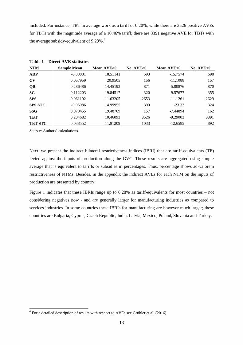
included. For instance, TBT in average work as a tariff of 0.20%, while there are 3526 positive AVEs

for TBTs with the magnitude average of a 10.46% tariff; there are 3391 negative AVE for TBTs with

the average subsidy-equivalent of 9.29%.6

Table 1 – Direct AVE statistics

NTM Sample Mean Mean AVE>0 No. AVE>0 Mean AVE<0 No. AVE<0

ADP -0.00081 18.51141 593 -15.7574 698

CV 0.057959 20.9505 156 -11.1088 157

QR 0.286486 14.45192 871 -5.80876 870

SG 0.112203 19.84517 320 -9.57677 355

SPS 0.061192 11.63205 2653 -11.1261 2629

SPS STC -0.05986 14.99955 399 -23.33 324

SSG 0.070455 19.48769 157 -7.44894 162

TBT 0.204682 10.46093 3526 -9.29003 3391

TBT STC 0.038552 11.91209 1033 -12.6585 892

Source: Authors’ calculations.

Next, we present the indirect bilateral restrictiveness indices (IBRI) that are tariff-equivalents (TE)

levied against the inputs of production along the GVC. These results are aggregated using simple

average that is equivalent to tariffs or subsidies in percentages. Thus, percentage shows ad-valorem

restrictiveness of NTMs. Besides, in the appendix the indirect AVEs for each NTM on the inputs of

production are presented by country.

Figure 1 indicates that these IBRIs range up to 6.28% as tariff-equivalents for most countries – not

considering negatives now - and are generally larger for manufacturing industries as compared to

services industries. In some countries these IBRIs for manufacturing are however much larger; these

countries are Bulgaria, Cyprus, Czech Republic, India, Latvia, Mexico, Poland, Slovenia and Turkey.

6 For a detailed description of results with respect to AVEs see Grübler et al. (2016).

14

Figure 1 – Average IBRI – accumulated BRI on inputs by country

Source: wiiw calculations.

Despite positive indirect accumulative tariffs on inputs (see Figure 3 in the appendix) the average

IBRIs are negative for some countries (Figure 1). For instance, Canada on average benefits from the

global trade policy measures with average negative IBRIs including AVEs from both tariffs and

NTMs. This suggests that Canadian providers benefit from trade policy measures that promote the

trade of their inputs of production along the GVC. This happens for both Canadian services and non-

services sectors. On the other hand, Bulgarian suppliers incur larger losses for more expensive inputs

due to trade restrictive NTMs. While normal tariffs induce above 1% indirect tariffs (Figure 3 in the

appendix) to the Bulgarian inputs for manufacturing sectors, NTMs induce around 5% in average,

which in total make the average BRI on Bulgarian inputs to above 6%.

As mentioned above, no tariffs are levied against trade flows of services. However, service providers

are indirectly affected by the policy measures imposed against the non-services inputs for their

production. In general, services are less impacted due to no direct impacts and the lower linkages. For

some countries - such as Belgium - service inputs are promoted on average by the global trade policy

measures while the inputs for the manufacturing have become expensive due to such measures.

15

Figure 2 – Accumulated AVE on inputs by sectors (IBRIs), in TE %

Figure 2 shows the effects of the respective trade policy measures by industry. For instance, TBTs

improve the cost efficiency of the inputs for the production of electrical and optical equipment, while

SPS, tariffs, and average BRIs increase the costs of inputs for these industries. An interesting pattern

emerges for the services sectors, where the majority of BRIs and AVEs for NTMs show negative

16

signs (see figures in the appendix). In fact, while tariffs levied on manufacturing products increase the

costs of inputs for service providers, regulated NTMs reduce these costs. Market efficiency

regulations enhancing the information symmetries which are directed within TBTs are good examples

that can act in opposite direction of tariffs.

5 Impact on performance measures

The bilateral AVEs of NTMs imply different cost structures for the direct but also indirect users of

intermediate inputs.7 The higher cost of intermediate inputs does not necessarily harm production. For

instance, as argued earlier, a higher quality induced by qualitative regulations embodied within NTMs

along the GVC, could bring inputs of production with higher prices. However, such a higher quality

can reflect in either higher quality of final product or better production procedure. Both will result in

higher gross output, while the latter is caused by higher value-added, the former is caused by the

higher price for higher quality of final goods. In this section the relation between BRIs and IBRIs on

productivity growth is considered.

5.1 Methodological outline and data

As discussed above, IBRI indicates the extent to which intermediate inputs are affected by trade

policy measures. From a simple Cobb-Douglas function 𝑌𝑗ℎ𝑡 = Ψ𝑗ℎ𝑡𝐾𝑗ℎ𝑡𝛼 𝐿𝑗ℎ𝑡

𝛼 , Ψ > 0, 0 < 𝛼 < 1

(where, Y, Ψ, K, and L are output, technology, capital, and labour, respectively), and then taking first

differences of the logarithmic labour intensive form, we can obtain labour productivity growth as:

∆𝑦𝑗ℎ𝑡 = ∆Ψ𝑗ℎ𝑡 + 𝛼∆𝑘𝑗ℎ𝑡 (11)

where 𝑦𝑗ℎ𝑡 and 𝑘𝑗ℎ𝑡 are respectively logarithmic forms of output to labour (productivity) and capital

to labour ratios, and ∆𝜓𝑗ℎ𝑡 is the technological progress of industry h in country j at time t, which we

hypothesize to be a function of trade policy channels and the share of high-skill labour in the given

industry ∆𝜓𝑗ℎ𝑡 = 𝛾0𝑇𝑃𝑗ℎ𝑡 + 𝛾1𝐻𝑆𝑗ℎ𝑡.

Since the aforementioned AVE for an NTM on a given industry is a constant effect over the period,

we will analyse its impact on the period-averaged annual productivity growth. Plugging the

hypothesized technology growth function into equation (11), and using the initial productivity levels

to account for convergence, we use the following growth model in our econometric analysis:

7 NTMs also impact on trade flows as such which are not considered here.

17

∆𝑦𝑗ℎ = 𝛽0 + 𝛽1𝑦𝑗ℎ,𝑡0 + 𝛽2∆𝑘𝑗ℎ

+ 𝛽3𝐻𝑆𝑗ℎ + 𝛽4𝐷𝐵𝑅𝐼𝑖𝑗ℎ

+ 𝛽5𝐼𝐵𝑅𝐼𝑗ℎ + 𝛽6𝐵𝑅𝐼𝑗ℎ + 𝛾ℎ

+ 𝛾𝑖𝑗 + 𝜇𝑖𝑗ℎ (12)

where ∆𝑦𝑗ℎ is the average annual labour productivity growth of industry h in country j from 2002 to

2009, 𝑦𝑗ℎ,𝑡0 is the initial level of productivity in logarithmic form, ∆𝑘𝑗ℎ is the average annual growth

of capital to labour ratio, 𝐷𝐵𝑅𝐼𝑖𝑗ℎ includes the AVEs for nine types of NTMs and period-averaged

tariffs imposed by country i against sector h from country j; 𝐼𝐵𝑅𝐼𝑗ℎ refers to the indirect tariff

equivalents of nine types of NTMs and tariffs on the inputs of industry h in country j; 𝐵𝑅𝐼𝑗ℎ includes

import-weighted AVEs and tariffs imposed by country j on sector h; 𝛾ℎ and 𝛾𝑖𝑗 are respectively

industry and country-pair specific effects, and 𝜇𝑖𝑗ℎ is the error term. Since we have a cross section

data, we use normal OLS for the estimation of equation (12) with robust standard errors to correct for

possible heteroscedasticity.

Data on gross output (GO), value added (VA), employment (l), and sectorial deflator for the fourth

stage of analysis are obtained from the WIOD SEA data. Finally, we borrow a data compilation for

Preferential Trade Agreements (PTAs) as reported by the WTO.

5.2 Results

Let us summarize the results of this investigation. The estimation of equation (12) is separated into

two categories, services and non-services sectors. This separation is mainly done because no tariff

data are available for services. Intuitively, IBRI affect the intermediate inputs of production of

services sectors as well as non-services sectors.

For labour productivity, we use two measurements to study the issue. One is the real gross output

divided by employment, and the other is the real value added divided by employment. Sectorial value

added deflators and exchange rates are used to calculate the real values from the national currency

units. This constrains the period of analysis to 2009.

The results indicate that there is no impact of any trade policy measures of the aforementioned first

channel (i.e. DBRI) on productivity growth of domestic industries, thus, we present the estimation

results excluding them including the two other channels. Table 2 presents the estimation results of the

impact of BRI and IBRI on the average annual labour productivity growth. As discussed earlier, we

separate the estimations on services and non-services sectors, because there are no tariffs levied on

services sectors.

18

Table 2 – Direct and Indirect BRI Impact on Productivity Growth

Non-services Services

Dep. Var: ∆𝑦𝑗ℎ𝑉𝐴

∆𝑦𝑗ℎ𝐺𝑂

∆𝑦𝑗ℎ𝑉𝐴

∆𝑦𝑗ℎ𝐺𝑂

𝑦𝑗ℎ,2002 -0.80*** -2.95*** -1.18*** -1.15***

(0.11) (0.23) (0.11) (0.11)

𝐻𝑆𝑗ℎ 20.4*** 20.4*** 0.12 -0.094

(1.09) (1.32) (0.35) (0.35)

∆𝑘𝑗ℎ 9.38*** 4.97*** 19.3*** 9.78***

(0.49) (0.69) (0.87) (0.70)

BRI 0.00026 0.00074

(0.0010) (0.0012)

IBRI 0.29*** 0.32*** -0.55*** -0.37***

(0.024) (0.035) (0.046) (0.045)

Constant 2.75*** 0.78 2.80*** 6.13***

(0.34) (0.55) (0.18) (0.15)

N 25707 25707 29069 29069

R-sq 0.401 0.317 0.451 0.424

adj. R-sq 0.360 0.269 0.418 0.389

Sector FE Yes Yes Yes Yes

Bilateral FE Yes Yes Yes Yes

Robust standard errors in parentheses * p<0.1, ** p<0.05, *** p<0.01

Source: wiiw calculations.

Control variables show the expected effects on productivity growth. It is important to note that the

dependent variable is the average annual growth rate in percentages to make them comparable with

the BRI and IBRI that are also in percentages. Thus, we observe large coefficients of human physical

capital. Negative statistically significant coefficients of initial productivities indicate the convergence

of growth, meaning that sectors with lower initial productivity have larger average annual growth

during the period. Non-services sectors with larger average share of high-skill labour (HS) enjoy

larger productivity growth. Statistically positive significant coefficients of physical capital to labour

ratio growth indicate how labour productivity is enhanced by capital.

Results do not show a statistically significant impact of the BRIs imposed against the sector’s exports

on the average annual growth of labour productivity. This is consistent for both types of productivity

measures. We mentioned earlier that DBRI had also statistically insignificant coefficients, which

indicate that neither BRI faced by the exporting sector nor DBRI faced by the foreign competitors of

the given sector influences the growth of productivity.

However, coefficients are statistically significant for IBRI and are positive for commodities (non-

services) and for services. Thus, labour productivity growth is affected positively by the trade policy

measures imposed against the inputs of a given non-service sector. This effect is larger for the

productivity calculated using the real gross output (GO). While value-added is net of the inputs, we

still observe positive influence of input trade policy measures on the productivity. Concerning

19

services, results suggest that services sectors with larger average annual productivity growth are those

with smaller costs of inputs. Global trade policy measures reducing the price of inputs for service

providers lead them to be more productive during years.

As discussed earlier, different types of policy measures have diverse impact on trade flows for various

reasons and consequently affect the productivity differently. In Table 3, we present the estimation

results of labour productivity growth over various types of policy measures. Many of these policy

measures against the exporting sectors do not have any statistically significant impact on productivity

growth of the sectors. Not even bilateral tariffs influence the growth of productivity. Non-services

sectors whose export flows are hindered by ADP and SPS STC measures to a larger extent are the

ones with larger average annual labour productivity growth. In contrast, smaller productivity growth

is related to the non-services sectors whose exports are largely hampered by the CV and TBT STC

measures.

The interesting results in Table 3 are the diverse impact of trade policy measures against the inputs of

sectors on productivity growth. Statistically significant positive coefficients of ITBT and ISPS in non-

services sectors point at the positive influence of quality regulations embodied in these measures

further up the value chains. Large AVEs for TBT and SPS indicate trade restrictiveness of these

measures increasing the price of inputs for production. In spite of higher costs of inputs induced by

these measures, VA productivity growth is improved. While ISPS increases also GO productivity

growth, ITBT does not influence GO productivity growth significantly. Robustness checks8 indicate

that excluding the initial GO productivity result in statistically significant positive coefficients for

ITBT. In fact, ITBT is negatively related with the initial GO productivity. These results point towards

the fact that TBTs hit the inputs of the least productive sectors at the beginning of the period much

more effectively, and induce them to be more productive in VA terms. Nevertheless, ITBT and ISPS

are negatively linked with the labour productivity growth of services sectors. This might point at the

shortcoming of these regulations in favour of services. Indirect cumulative AVEs for ADPs against

the inputs of non-services sectors have also positive impact on the productivity growth. While the

increased prices of inputs by ADP are linked with larger VA productivity growth of services, they are

related to lower growth of labour productivity calculated using GO.9

8 Robustness checks can be provided up on request.

9 This puzzling role of ADP was also highlighted in other studies such as Ghodsi, Jokubauskaite, and Stehrer

(2015)

20

Table 3 – Direct and Indirect Policy Measures Impact on Productivity Growth Non-services Services

Dep. Var: ∆𝑦𝑗ℎ𝑉𝐴

∆𝑦𝑗ℎ𝐺𝑂

∆𝑦𝑗ℎ𝑉𝐴

∆𝑦𝑗ℎ𝐺𝑂

𝑦𝑗ℎ,2002 -0.85*** -2.98*** -1.14*** -1.21***

(0.11) (0.23) (0.11) (0.12)

𝐻𝑆𝑗ℎ 20.8*** 20.8*** 0.10 -0.29

(1.12) (1.35) (0.36) (0.36)

∆𝑘𝑗ℎ 9.68*** 5.46*** 19.7*** 10.0***

(0.49) (0.70) (0.89) (0.71)

ADP 0.0076** 0.0062*

(0.0031) (0.0034)

CV -0.029*** -0.012

(0.0088) (0.0083)

QR -0.0055 -0.0044

(0.0039) (0.0044)

SG 0.0012 0.0030

(0.0047) (0.0049)

SPS -0.00087 0.00034

(0.0022) (0.0025)

SSG 0.0022 -0.0038

(0.0067) (0.0082)

TBT 0.00029 -0.00092

(0.0025) (0.0034)

TBTSTC -0.0054* -0.0031

(0.0033) (0.0035)

SPS STC 0.015*** 0.017***

(0.0030) (0.0033)

Tariffs 0.0035 0.0032

(0.0047) (0.0061)

IADP 0.64*** 0.29*** 0.91*** -1.47***

(0.061) (0.071) (0.17) (0.17)

ICV -0.099 -0.023 -1.33*** -0.011

(0.093) (0.100) (0.36) (0.30)

IQR 0.15 -0.53** -0.35* -0.91***

(0.22) (0.21) (0.19) (0.25)

ISG -0.086 -0.18 0.61 -1.23**

(0.093) (0.14) (0.57) (0.54)

ISPS 0.58*** 0.70*** -1.31*** -0.89***

(0.048) (0.078) (0.068) (0.071)

ISSG -0.57 0.056 -3.09*** -1.41***

(0.36) (0.51) (0.23) (0.25)

ITBT 0.31*** -0.020 -1.88*** -1.93***

(0.047) (0.044) (0.18) (0.19)

ITBT STC -0.27*** -0.42*** 2.02*** 2.87***

(0.063) (0.10) (0.29) (0.32)

ISPS STC 0.80*** 1.66*** -1.81*** 1.14*

(0.12) (0.18) (0.57) (0.62)

ITariffs -0.092*** 0.44*** 0.45*** 1.16***

(0.034) (0.071) (0.072) (0.076)

Constant 2.66*** 0.56 3.19*** 4.93***

(0.35) (0.54) (0.20) (0.21)

N 25707 25707 29069 29069

R-sq 0.407 0.322 0.456 0.432

adj. R-sq 0.365 0.275 0.423 0.397

Sector FE Yes Yes Yes Yes

Bilateral FE Yes Yes Yes Yes

Robust standard errors in parentheses * p<0.1, ** p<0.05, *** p<0.01

High costs of inputs induced by QR do not significantly affect the VA productivity growth of non-

services sectors. IQR mainly influence the GO productivity growth, which shows no relevant role of

these measures in qualitative performance of industries. Despite no influence of SG and SSG on the

productivity growth of non-services sectors, the results indicate a negative relationship between these

measures and services labour productivity growth.

Governments raise STCs on TBTs that are more trade restrictive harming their domestic industries

(Ghodsi, 2015a). ITBT STC coefficients point at a similar intuition that higher costs of inputs induced

21

by trade restrictive TBT STCs are linked with smaller annual productivity growth of non-services

sectors. However, the TBT STC-induced higher prices of inputs increase the productivity growth of

services. Cumulative AVEs of SPS STCs incurring higher costs of inputs are linked with larger

productivity growth of non-services sectors. However, they are linked with lower VA productivity

growth of services sectors.

Another interesting result concerns the impact of indirect tariffs on inputs. Despite the small

magnitude of tariffs incurred along the GVCs due to liberalization process, manufacturers are affected

by them statistically significantly. Positive coefficient for the GO productivity growth and negative

coefficient for the VA productivity growth mainly indicate that producers increase their price of

products and services due to higher costs of inputs. However, this is a burden on non-services

industries leading to lower VA productivity growth.

6 Conclusions

In this paper we track the non-tariff measures (NTMs) and study how they trickle through the global

value chains (GVCs). The importance of the NTMs as complex trade policy measures is highlighted

in various studies of the international trade policy literature. The opaque nature of NTMs

distinguishes them from normal tariffs since they have qualitative impact on products flows in

addition to price effects. While price effects incurred further up the value chains can be easily tracked

along GVC, impact of NTMs on quality of upper stream sectors influence the production processes

along GVC. In this paper, we present a framework to quantify such impacts.

In a four-stage approach we estimate the trickling down effect of NTMs and tariffs on labour

productivity growth. The first stage estimates the bilateral import demand elasticities applying a semi-

flexible translog GDP function using detailed 6-digit bilateral trade flows. The second stage quantifies

the bilateral ad-valorem equivalents (AVE) of nine types of NTMs notified to the World Trade

Organization (WTO) until 2011 applying a structural gravity model on traded quantities and using the

elasticities calculated in previous stage for the period 2002-2011. The third stage uses these estimated

AVEs of the various types of NTMs and the average tariffs for the period to calculate the cumulative

indirect bilateral-trade restrictiveness indices (IBRI) for the inputs of production applying the Leontief

technical coefficients consistent with WIOD. Three channels of trade policy measures are discussed

as possible channels affecting the performance of industries. The first channel affects the foreign

competitors of a given industry through direct trade protectionism measures (DBRI). Second channels

are considered to be IBRI. Third channel is discussed as trade policy measures faced by the exports of

a given sector (BRI). The final stage of the paper analyses the impact of these three channels of trade

policy measures on the average annual labour productivity growth.

The contribution of this paper is two-fold. We firstly provide a database for bilateral AVEs of NTMs.

This contributes to the existing literature in different ways: a dataset on bilateral AVEs for nine types

22

of NTM notified to the WTO during a period based on their intensity is a major contribution of this

paper. Secondly, we explain labour productivity growth by various types of global trade policy

measures incorporated along the GVC. The results point towards a positive influence of regulations

embodied within TBTs and SPS further up the value chains on the performance of non-services

industries. Moreover, diverse effects of different types of NTMs are in line with the existing argument

within the literature on complexity of these trade policy tools.

23

Bibliography

Antràs, P., Chor, D., Fally, T., & Hillberry, R. (2012). Measuring the Upstreamness of Production and

Trade Flows. The American Economic Review, 102(3), 412-416.

Backer, K. D. and S. Miroudot (2013), “Mapping Global Value Chains”, OECD Trade Policy Papers,

No. 159, OECD Publishing. http://dx.doi.org/10.1787/5k3v1trgnbr4-en

Bair, J. (2005). Global capitalism and commodity chains: looking back, going forward. Competition

& Change, 9(2), 153-180.

Baltagi, B. H., Egger, P., & Pfaffermayr, M. (2003). A generalized design for bilateral trade flow

models. Economics Letters, 80(3), 391-397.

Beghin, J., Disdier, A. C., & Marette, S. (2014). Trade Restrictiveness Indices in Presence of

Externalities: An Application to Non-Tariff Measures.

Beghin, J., Disdier, A. C., Marette, S., & Van Tongeren, F. (2012). Welfare costs and benefits of non-

tariff measures in trade: a conceptual framework and application. World Trade Review,

11(03), 356-375.

Bratt, M. (2014). Estimating the bilateral impact of non-tariff measures (NTMs) (No. 14011). Institut

d'Economie et Econométrie, Université de Genève.

Caves, D. W., Christensen, L. R., & Diewert, W. E. (1982). Multilateral comparisons of output, input,

and productivity using superlative index numbers. The economic journal, 73-86.

Cое, D. T., Helpman, E., & Hoffmaister, A. W. (1997). North-South R&D Spillovers. Economic

Journal, 107(440), 134-49.

de Almeida, F. M., da Cruz Vieira, W., & da Silva, O. M. (2012). SPS and TBT agreements and

international agricultural trade: retaliation or cooperation?. Agricultural Economics, 43(2),

125-132.

Edwards, S. (1998). Openness, productivity and growth: what do we really know?. The economic

journal, 108(447), 383-398.

Foster-McGregor, N., Pöschl, J., & Stehrer, R. (2014). Capacities and Absorptive Barriers for

International R&D Spillovers through Intermediate Inputs (No. 108). The Vienna Institute for

International Economic Studies, wiiw.

Frankel, J. A., & Romer, D. (1999). Does trade cause growth?. American economic review, 379-399.

Gereffi, G. (1994) The organization of buyer-driven global commodity chains: how US retailers shape

overseas production networks, in G. Gereffi and M. Korzeniewicz (eds) Commodity Chains

and Global Capitalism (Westport, CT, Praeger).

Gereffi, G., & Sturgeon, T. (2013). Global Value Chain-Oriented Industrial Policy: The Role of

Emerging Economies. In Elms, D. K., & Low, P. (Eds.) Global value chains in a changing

world. Geneva: World Trade Organization.

Gereffi, G., Humphrey, J., & Sturgeon, T. (2005). The governance of global value chains. Review of

international political economy, 12(1), 78-104.

Ghodsi, M. (2015a). Determinants of Specific Trade Concerns Raised on Technical Barriers to Trade

(No. 115). The Vienna Institute for International Economic Studies, wiiw.

24

Ghodsi, M., Grübler, J., & Stehrer, R., (2015) “The impact of NTMs on imports”, Paper written in the

PRONTO project, work in progress

Ghodsi, M., Jokubauskaite, S., & Stehrer, R., (2015) “Non-Tariff Measures and the quality of

imported products”, Paper written in the PRONTO project, work in progress

Ghodsi, M., Reiter, O., & Stehrer, R. (2015) Compilation of a Database for Non-Tariff Measures from

the WTO Integrated Trade Intelligence Portal (WTO I-TIP), Paper written in the PRONTO

project, work in progress

Ghodsi, M., Stehrer, R. (2015). Which country of origin is preferable? Using new estimates for

bilateral import demand elasticities, Paper written in the PRONTO project, work in progress.

Grossman, G. M., & Helpman, E. (1993). Innovation and growth in the global economy. MIT press.

Hagemejer, J., & Ghodsi, M. (2014). Up or down the value chain? The comparative analysis of the

GVC position of the CEECs economies.

Harrison, A. (1996). Openness and growth: A time-series, cross-country analysis for developing

countries. Journal of development Economics, 48(2), 419-447.

Hopkins, T. K., & Wallerstein, I. (1977). Patterns of development of the modern world-system.

Review (Fernand Braudel Center), 111-145.

Kee, H. L., Nicita, A., & Olarreaga, M. (2008). Import demand elasticities and trade distortions. The

Review of Economics and Statistics, 90(4), 666-682.

Kee, H. L., Nicita, A., & Olarreaga, M. (2009). Estimating trade restrictiveness indices*. The

Economic Journal, 119(534), 172-199.

Lumenga-Neso, O., Olarreaga, M., & Schiff, M. (2005). Onindirect'trade-related R&D spillovers.

European Economic Review, 49(7), 1785-1798.

Miroudot, S., D. Rouzet and F. Spinelli (2013), “Trade Policy Implications of Global Value Chains:

Case Studies”, OECD Trade Policy Papers, No. 161, OECD Publishing.

http://dx.doi.org/10.1787/5k3tpt2t0zs1-en

Moore, M. O., & Zanardi, M. (2011). Trade Liberalization and Antidumping: Is There a Substitution

Effect?. Review of Development Economics, 15(4), 601-619.

Nishioka, S., & Ripoll, M. (2012). Productivity, trade and the R&D content of intermediate inputs.

European Economic Review, 56(8), 1573-1592.

OECD. Publishing. (2013). Interconnected Economies: Benefiting from Global Value Chains. OECD

Publishing.

Otsuki, T., Wilson, J. S., & Sewadeh, M. (2001). Saving two in a billion:: quantifying the trade effect

of European food safety standards on African exports. Food policy, 26(5), 495-514.

Porter, M. E. (1985). Competitive advantage: creating and sustaining superior performance, 1985.

Rodriguez, F., & Rodrik, D. (2001). Trade policy and economic growth: a skeptic's guide to the cross-

national evidence. In NBER Macroeconomics Annual 2000, Volume 15 (pp. 261-338). MIT

Press.

Rosendorff, B. P. (1996). Voluntary export restraints, antidumping procedure, and domestic politics.

The American economic review, 544-561.

25

Rouzet, D., & Miroudot, S. (2013, June). The Cumulative Impact of Trade Barriers Along The Value

Chain: An Empirical Assessment Using the OECD Inter-Country Input-Output Model'. In

16th Annual Conference on Global Economic Analysis. According to a similar logic, the

cumulative tariff on services value-added for on an.

Sanjuán López, A. I., Philippidis, G., & Resano Ezcaray, H. (2013). Gravity estimation of non tariff

measures (NTMs) on EU-USA agri-food trade: Implications for further analysis.

Sraffa, P. (1975). Production of commodities by means of commodities: Prelude to a critique of

economic theory. CUP Archive.

Timmer, M., Erumban, A. A., Gouma, R., Los, B., Temurshoev, U., de Vries, G. J., etc.. & Pindyuk,

O. (2012). The world input-output database (WIOD): contents, sources and methods (No.

20120401). Institue for International and Development Economics.

Vandenbussche, H., & Zanardi, M. (2008). What explains the proliferation of antidumping laws?,

Economic Policy, 23(53), 94-138.

26

Appendix

27

Figure 3 – Average Indirect Tariffs on Inputs by Country

Figure 4 – Average tariff-equivalent (TE) for TBT on Inputs by Country

28

Figure 5 - Average TE for TBT on Inputs by Country

Figure 6 - Average TE for TBT STC on Inputs by Country

29

Figure 7 - Average TE for SPS STC on Inputs by Country

Figure 8 - Average Te for ADP on Inputs by Country

30

Figure 9 - Average TE for CV on Inputs by Country

Figure 10 - Average TE for QR on Inputs by Country

31

Figure 11 – Average TE for SG on Inputs by Country

Figure 12 - Average TE for SSG on Inputs by Country