nonautonomous discrete bright soliton solutions and...
TRANSCRIPT

PHYSICAL REVIEW E 91, 032914 (2015)
Nonautonomous discrete bright soliton solutions and interactionmanagement for the Ablowitz-Ladik equation
Fajun Yu*
School of Mathematics and Systematic Sciences, Shenyang Normal University, Shenyang 110034, China(Received 25 November 2014; revised manuscript received 28 January 2015; published 19 March 2015)
We present the nonautonomous discrete bright soliton solutions and their interactions in the discrete Ablowitz-Ladik (DAL) equation with variable coefficients, which possesses complicated wave propagation in time anddiffers from the usual bright soliton waves. The differential-difference similarity transformation allows us to relatethe discrete bright soliton solutions of the inhomogeneous DAL equation to the solutions of the homogeneousDAL equation. Propagation and interaction behaviors of the nonautonomous discrete solitons are analyzedthrough the one- and two-soliton solutions. We study the discrete snaking behaviors, parabolic behaviors, andinteraction behaviors of the discrete solitons. In addition, the interaction management with free functions anddynamic behaviors of these solutions is investigated analytically, which have certain applications in electricaland optical systems.
DOI: 10.1103/PhysRevE.91.032914 PACS number(s): 05.45.Yv, 67.85.Hj, 03.75.Kk, 03.75.Lm
I. INTRODUCTION
In nonlinear science, the study of nonlinear differential-difference equations (DDEs) has aroused increasing interest.DDEs are frequently used to model a wide variety ofcomplicated physical phenomena such as particle vibrationsin lattices, currents flow in electrical networks, and pulses inbiological chains [1–3].
The most efficient ones are the Ablowitz-Kaup-Newel-Segur (AKNS) method and Ablowitz-Ladik (AL) method [4],that are based on the Zakharov and Shabat spectral problem.The AL hierarchy is a set of integrable discrete nonlineardynamic systems. It is known that AL hierarchy has a variety ofmodeling applications including optics [5,6] and chaos in dis-persive numerical schemes [7,8]. There are many publicationsrelating to the AL equation and discrete systems. In particular,the integrable discrete Ablowitz-Ladik (DAL) equation hascertain electrical and optical systems [8–10]. Reference [8]has shown that a discrete electrical lattice employing theinductors and nonlinear capacitors in a transmission line can bedescribed by a model which incorporates the AL equation withthe discrete-self-trapping models. Reference [9] has given anoverview of a more general system that combines the AL equa-tion with other discrete nonlinear Schrodinger (DNLS)-typeequations with some applications to optical and electrical sys-tems. By means of the Backlund transformation, the AL equa-tion has been converted to a physically corrected twin modelwith the application to the Peierls-Nabarro problem [11].
Since Ablowitz and Ladik introduced the discrete ALequation [5,12], some methods have been proposed to solvethe nonlinear discrete soliton equations in Refs. [5,12–16].For example, there is research conducted for soliton solutions,the Backlund transformation, the Darboux transformation,Hamiltonian structures, conserved quantities, and other prop-erties. The authors of Refs. [17–20] discuss quasiperiodicsolutions for the AL equations, which include the discretenonlinear Schrodinger (NLS) equation and the discrete mod-ified Korteweg-de Vries (mKdV) equation. Seeking and the
investigation of the exact solutions are crucial tasks in the studyof nonlinear DDEs. Especially, the discrete soliton solutionswhich are intrinsic highly localized models of a nonlinearlattice have been demonstrated to exist in a wide range ofdiscrete physical systems [21,22].
Recently, some important scientific studies of the nonau-tonomous NLS equations were derived. Serkin and Hasegawaconsider a systematic way to find an infinite number of thestable bright and dark solitons of the NLS equation withvarying dispersion, nonlinearity, and gain or absorption in [23].And, the different soliton management regimes are predictedin [24]. The nonautonomous NLS equations with linear andharmonic oscillator potentials are introduced in [25]; thenonautonomous solitons that interact elastically in externalpotentials are demonstrated in this system. Furthermore, theexact analytical solutions and numerical experiments revealmany specific features of nonautonomous solitons in [26].
In particular, the discrete rogue wave (DRW) can beused as spatial energy concentrators in arrays of a nonlinearwaveguide. And, the DRW solutions may well find practicalapplications. However, there are few reports to date about thenonautonomous DRW except for the discrete NLS equation[27,28], the AL lattice equation [12,29], and the discrete Hirotaequation [30]. Yan and Jiang explore exact nonautonomousDRW solutions and interaction of the generalizedAblowitz-Ladik-Hirota (ALH) lattice equation with variablecoefficients [31]. The discrete NLS equation is nonintegrable,which has some interesting applications in physics [9,32,33].The AL lattice equation is integrable and possesses an infinitenumber of conservation laws [12,29], which is used to studysome properties of the intrinsic localized modes [34].
Although many people have investigated the discreteintegrable AL equation [10,35,36], however few people havestudied the soliton dynamics with the free function effects. Thediscrete rogue wave solutions have been given in Ref. [31].Different from those works in the previous studies, wefurther extend the investigation to the exact nonautonomousdiscrete bright soliton solutions and their interactions of theDAL equation with variable coefficients in this paper. Someexplicit solutions of the DAL equation with potentials andnonlinearities depending on both time and spatial coordinates
1539-3755/2015/91(3)/032914(8) 032914-1 ©2015 American Physical Society

FAJUN YU PHYSICAL REVIEW E 91, 032914 (2015)
are considered. We also exhibit the wave propagation ofnonautonomous discrete bright soliton (DBS) solutions andtheir interaction management for some chosen parameters andfunctions. For the given periodic gain or loss term, when theamplitude of the tunnel coupling coefficient between sitesincreases, these nonautonomous DBS solutions are localized inspace and appear with some discrete behaviors, which are quitedistinct from the well-known shaped one presented before. Wehope that the time-space scale extension of the AL hierarchywill give a wider range of integrable dynamic systems thatcould be used in modeling.
The rest of this paper is organized as follows. In Sec. II, wedescribe the differential-difference similarity reductions of theDAL equation. In Sec. III, we present several types of exactnonautonomous DBS solutions, consider the propagation andinteraction behaviors, and then the interaction managementwith free functions of these solutions is investigated analyti-cally. Finally, we give some Conclusions.
II. DIFFERENTIAL-DIFFERENCE SIMILARITYREDUCTIONS AND CONSTRAINTS
We here address the DAL equation with variable coeffi-cients modeled by the following lattice form
i�nt =(
1
h2+ g(t)|�n|2
)[�(t)�n+1 + �∗(t)�n−1]
− 2
h2vn(t)�n + iγ (t)�n, (1)
where �n = �n(t) stands for the complex field amplitude atthe nth site of the lattice, the complex-valued function �(t)is the coefficient of tunnel coupling between sites and canbe rewritten as �(t) = a1(t) + ia2(t), with a1(t) and a2(t)being differentiable, the real-valued function g(t) stands for thetime-modulated interstice nonlinearity, vn(t) is the space-timemodulated inhomogeneous frequency shift, and γ (t) denotesthe time-modulated effective gain or loss term.
In fact, this nonlinear lattice model (1) contains manyspecial lattice models, such as the generalized Ablowitz-Ladik-Hirota lattice for the case h = 1 [31], the AL latticefor the case h = 1, a1(t) = const, a2(t) = vn(t) = γ (t) = 0,and g(t) = const [28,29], the AL equation with an additionalterm accounting for dissipation in the case h = 1, a1(t) =const, a2(t) = vn(t) = 0, γ (t) = const, and g(t) = const [37],the discrete Hirota equation for the case h = 1, a1(t) =const, a2(t) = const,vn(t) = γ (t) = 0, and g(t) = const [38],the generalized AL lattice given by Eq. (1) for the casea1(t) = const, a2(t) = γ (t) = 0, and g(t) = const [39], andthe discrete mKdV equation for the case a1(t) = vn(t) =γ (t) = 0, a2(t) = const, and g(t) = const [40].
We consider spatially localized solutions of Eq. (1), i.e.,limn→∞ �n(t) = 0. We search for a proper similarity transfor-mation connecting solutions of Eq. (1) with those solutions ofthe following DAL equation with constant coefficients [41],which is a third-order lattice equation
i�nτ =(
1
h2+ |�n|2
)(λ�n+1 + λ∗�n−1) − 2
h2Re(λ)�n,
(2)
where �n = �n(τ ) is a physical field of space n, and the τ =τ (t) is a real-valued function of time to be determined, and thecomplex-valued parameter λ can be rewritten as λ = a + ib
with a and b being real-valued parameters. The third-orderdiscrete model (2) contains some special physical models,such as the AL lattice for the case h = 1, a = 1, and b = 0[12,29], the discrete mKdV equation for the case h = 1, a = 0,and b = 1 [40], and the discrete Hirota equation for the caseh = 1 [31].
The DAL equation (1) provides the means to describeanalytically various dynamical regimes of the N -soliton trainand to predict initial soliton parameters responsible for eachof the regimes, and the numerical simulations corroboratewell analytical predictions [10]. An interesting problemof the characterization of solitons present in numerical orexperimental data has been discussed by Boiti et al. [42] inthe context of a train of envelope wave pulses modeled bythe AL equation on a finite interval. Experimentally, it studiesa discrete electrical lattice where the dynamics of modulatedwaves can be modeled by the DAL equation (1). Regions ofmodulational instability (MI) are investigated; it is shown thatunlike envelope solitons, which can be observed close to thezero-dispersion point, the staggered modes experience stronglattice effects. Some results are confirmed by the observationof “staggered” localized modes. Another, the analytical andnumerical investigations of MI of the AL equation, showingnonlinear development of the instability as well as spatialstructures, are displayed in [43].
It has been reported that solitons could collide inelastically,and there are shape-changing collisions for a discrete system(2). In this paper, we will solve Eq. (1) with nontrivial seedsolutions and study the nonautonomous DBS solutions with atrivial background.
According to the ansatz methods [31,44,45], we search forthe solutions of the physical field
�n(t) = ρ(t)eiϕn(t)�n(τ (t)), (3)
where ρ(t) and ϕn(t) are the real-value functions of theindicated variables.
To conveniently substitute ansatz (3) into Eq. (1)and to further balance the phases in every term, i.e.,�n(t),�n+1(t),�n−1(t) in Eq. (1), we should first know theexplicit expression of the phase in space. Similar to the phasesin the discrete Hirota equation [31], we here consider the casethat the phase is expressed as a cubic polynomial in space andits coefficients are the functions of time in the following form:
ϕn(t) = p3(t)n3 + p2(t)n2 + p1(t)n + p0; (4)
based on symmetry analysis, we simply balance the coeffi-cients of these terms �n(t), �n+1(t), and �n−1(t) such thatwe find that the phase in transformation (4) should be a firstdegree polynomial in space with coefficients being functionsof time, namely,
ϕn(t) = p1(t)n + p0(t), (5)
where p0(t), p1(t), p2(t), and p3(t) are functions of time to bedetermined.
Equation (3) allows us to reduce Eq. (1) to Eq. (2);the variables in this reduction can be determined from therequirement for the physical field �n(τ (t)) to satisfy Eq. (2).
032914-2

NONAUTONOMOUS DISCRETE BRIGHT SOLITON . . . PHYSICAL REVIEW E 91, 032914 (2015)
Thus, we substitute transformation (3) into Eq. (1) and afterrelatively simple algebra obtain the system of nonlinear partialdifferential equations; we get the following system:
ρ(t) + γ (t)ρ(t) = 0, g(t)ρ2(t) = 1,
2vn(t) = 2aτ (t) − h2[p1(t)n + p0(t)],
aτ (t) − a1(t) cos p1(t) + a2(t) sin p1(t) = 0,
[ba1(t) − aa2(t)] cos p1(t)
−[aa1(t) + ba2(t)] sin p1(t) = 0, (6)
where the dot denotes the derivative with respect to time.Therefore, if system (6) is consistent, we can construct analgorithm generating nonautonomous DBS solutions of Eq. (1)based on transformation (3) and Eq. (2): First, we solve Eq. (6)to obtain the functions ρ(t),τ (t), and p1(t) in transformation(3). Second, we consider Eq. (6) to determine the externalpotential vn(t) and nonlinearity g(t) in Eq. (1) in terms of theabove-obtained functions ρ(t),τ (t), and p1(t). Last, we haveestablished a transformation (3) connecting solutions of Eq. (2)and those solutions of Eq. (1). In particular, we here exhibitour approach in terms of two lowest-order DBS solutions ofEq. (2) as seed solutions to find nonautonomous DBS solutionsof Eq. (1).
Solving Eq. (6), we get the similarity variables ρ(t),τ (t),and p1(t) in the form:
ρ(t) = ρ0e− ∫ t
c1γ (s)ds
,
p1(t) = tan−1
⌈ba1(t) − aa2(t)
aa1(t) + ba2(t)
], (7)
τ (t) = (a2 + b2)12
∫ t
c2
[a2
1(s) + a22(s)
] 12 ds,
where c1,c2 are constants, s is an integration variable, and ρ0
is an integration constant. Now it follows from Eq. (6) that wefurther find the external potential vn(t) and nonlinearity g(t)with c1,c2 chosen as zero in the following form:
g(t) = 1
ρ20
e2∫ t
0 γ (s)ds,
(8)vn(t) = v1(t)n + v0(t),
where we introduce two functions in external potential vn(t)in the form:
v1(t) = −h2 p1(t)
2,
v0(t) = −h2 p0(t)
2+
[a2
1(t) + a22(t)
a2 + b2
] 12
. (9)
We choose the different parameters h,a,b and the differentfunctions a1(t), a2(t), γ (t); the Fig. 1 depicts the profiles ofnonlinearity g(t), τ (t) and the external potential v1(t) given byEqs. (7), (8), and (9).
III. NONAUTONOMOUS DBS SOLUTIONS ANDINTERACTION MANAGEMENT
Although many people have investigated the discreteintegrable AL equation, few people have studied the soliton
(a)
(b)
(c)
FIG. 1. (Color online) Profiles of (a) nonlinearity v1(t) is givenby Eq. (9) with a1(t) = sin(t), a2(t) = cos (3t), a = 1, b = 1, h = 1;(b) g(t) is given by Eq. (8) with γ (t) = sin(t) sin(2t), ρ0 = 1; (c) thefunction τ (t) is given by Eq. (7) with a1(t) = sin(3t), a2(t) = 0, a =1, b = 1.
dynamics of controllable interactions with free functions.Different from that work in the previous studies, we will aim toanalyze the soliton dynamics of Eq. (1) with the managementeffects of a1(t),a2(t), and γ (t), based on the DBS solutions.
In order to control the soliton interactions, we consider theanalysis of functions a1(t),a2(t), and γ (t). The results havesome guiding significance for controllable management of asoliton, and can provide some theoretical analysis for carryingout optical soliton communication experiments.
032914-3

FAJUN YU PHYSICAL REVIEW E 91, 032914 (2015)
A. Nonautonomous discrete one-bright soliton solution
In Ref. [46], the N -bright soliton solutions are obtainedvia the Hirota bilinear method for a discrete integrable ALequation (2).
Based on the similarity transformation (4) and the brightsoliton solutions of the Eq. (2) in [46], we present thenonautonomous discrete one-bright soliton solution of Eq. (1)
(a)
(b)
(c)
FIG. 2. (Color online) Profiles of (a) the intensity distribu-tion |� (1)
n (t)| with k = 0.8, h = 1, a = 1, b = 1, γ (t) = −6 sin(t)cos5(t), ρ0 = 1; (b) the intensity distribution |� (1)
n (t)| for t =0 [the blue (left) line], t = 0.5 [the red (middle) line], t = 2[the green (right) line]; (c) the intensity distribution |� (1)
n (t)|with the parameters as k = 1, h = 1, a = 1, b = 1, a1(t) = a2(t) =1−2t√
2, γ (t) = −sin(t) cos(t), ρ0 = 1 in Eq. (10).
in the form:
�(1)n (t) = ρ0e
− ∫ t
0 γ (s)ds+i[p1(t)n+p0+ϕn(τ (t))]
× (i)n
2exp
(θ−θ∗ − ln B
2
)sech
(θ+θ∗+ln B
2
),
(10)
where B = h2
4 sinh−2( k+k∗2 ), θ = kn + ωτ,ω = −2i−2 sinh(k)
h2 ,
and ϕn(τ (t)) = 2τ (t)[2√
a2 + b2 − a] − n tan−1 ba
, τ (t) =(a2 + b2)
12∫ t
c2[a2
1(s) + a22(s)]
12 ds [the variable τ (t) is given by
Eq. (7)]; and the phase ϕn(t) = p1(t)n + p0(t), p1(t) is given
(a)
(b)
(c)
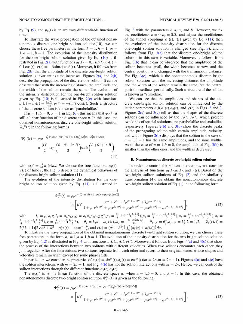
FIG. 3. (Color online) Profiles of (a) the intensity dis-tribution |� (1)
n (t)| with k = 1.5 + i,h = 1,a = 1,b = 0,a1(t) =0.01sin(t),γ (t) = sin(t),ρ0 = 0.1; (b) the intensity distribution|� (1)
n (t)| for t = 0 [the blue (upper) line], t = 1 [the red (mid-dle) line], t = 2 [the green (lower) line]; (c) the intensity dis-tribution |� (1)
n (t)| with k = 0.8,h = 1,a = 1,b = 0,a1(t) = 0.15 −0.01t2,γ (t) = −0.1cos(t),ρ0 = 1 in Eq. (11).
032914-4
NONAUTONOMOUS DISCRETE BRIGHT SOLITON . . . PHYSICAL REVIEW E 91, 032914 (2015)
by Eq. (9), and p0(t) is an arbitrary differentiable function oftime.
To illustrate the wave propagation of the obtained nonau-tonomous discrete one-bright soliton solution(10), we canchoose these free parameters in the form k = 1, h = 1, ρ0 =1, a = 1, b = 1. The evolution of the intensity distributionfor the one-bright soliton solution given by Eq. (10) is il-lustrated in Fig. 2(a) with functions a1(t) = 0.1 sin(t), a2(t) =0.1 cos(t), γ (t) = −6 sin(t) cos5(t). Moreover, it follows fromFig. 2(b) that the amplitude of the discrete one-bright solitonsolution is invariant as time increases. Figures 2(a) and 2(b)describe the propagation of the discrete one-soliton. It can beobserved that with the increasing distance, the amplitude andthe width of the soliton remain the same. The evolution ofthe intensity distribution for the one-bright soliton solutiongiven by Eq. (10) is illustrated in Fig. 2(c) with functionsa1(t) = a2(t) = 1−2t√
2,γ (t) = −sin(t)cos(t). Such a structure
of the discrete soliton is known as “parabolalike.”If a = 1, b = 0, λ = 1 in Eq. (6), this means that ϕn(t) is
still a linear function of the discrete space n. In this case, theobtained nonautonomous discrete one-bright soliton solution�(1)
n (t) in the following form is
�(1)n (t) = ρ0e
− ∫ t
0 γ (s)ds+i[p1(t)n+p0+2{∫ t
c2[a2
1 (s)+a22 (s)]
12 ds}]
× (i)n
2exp
(θ−θ∗−ln B
2
)sech
(θ+θ∗+ln B
2
),
(11)
with τ (t) = ∫ t
0 a1(s)ds. We choose the free functions a1(t),γ (t) of time t ; the Fig. 3 depicts the dynamical behaviors ofthe discrete-bright soliton solution (11).
The evolution of the intensity distribution for the one-bright soliton solution given by Eq. (11) is illustrated in
Fig. 3 with the parameters k,ρ0,a, and b. However, we fixthe coefficients k = 0,ρ0 = 0.5, and adjust the coefficientsof the tunnel couplings a1(t),γ (t) given by Eq. (11); thenthe evolution of the intensity distribution for the discreteone-bright soliton solution is changed (see Fig. 3), and itfollows from Fig. 3(a) that the discrete one-bright solitonsolution in this case is variable. Moreover, it follows fromFig. 3(b) that it can be observed that the amplitude of thesoliton becomes small, the width becomes narrow, and thecentral position is unchanged with the transmission distance.For Fig. 3(c), which is the nonautonomous discrete brightsoliton solution with the increasing distance, the amplitudeand the width of the soliton remain the same, but the centralposition oscillates periodically. Such a structure of the solitonis known as “snakelike.”
We can see that the amplitudes and shapes of the dis-crete one-bright soliton solution can be influenced by thelattice parameters a,b,a1(t),a2(t), and γ (t) in Figs. 2 and 3.Figures 2(c) and 3(c) tell us that the shapes of the discretesolitons can be influenced by the a1(t),a2(t), which presenttwo kinds of special solutions: the parabolalike and snakelike,respectively. Figures 2(b) and 3(b) show the discrete peaksof the propagating soliton with certain amplitude, velocity,and width. Figure 2(b) displays that the soliton in the case ofa = 1,b = 1 has the same amplitudes, and the same widths.As to the case of a = 1,b = 0, the amplitude of Fig. 3(b) issmaller than the other ones, and the width is decreased.
B. Nonautonomous discrete two-bright soliton solutions
In order to control the soliton interactions, we considerthe analysis of functions a1(t),a2(t), and γ (t). Based on thetwo-bright soliton solutions of Eq. (2) and the similaritytransformation (4), we obtain the nonautonomous discretetwo-bright soliton solution of Eq. (1) in the following form:
�(2)n (t) = ρ0e
− ∫ t
0 γ (s)ds+i[p1(t)n+p0+ϕn(τ (t))]
×[
(i)neθ1 + eθ2 + l1e
θ1+θ2+θ∗1 + l2e
θ1+θ2+θ∗2
1 + ρ1eθ1+θ∗
1 + ρ2eθ1+θ∗
2 + ρ3eθ2+θ∗
1 + ρ4eθ2+θ∗
2 + �eθ1+θ∗1 +θ2+θ∗
2
], (12)
with l1 = ρ1ρ3χ,l2 = ρ2ρ4χ,� = ρ1ρ2ρ3ρ4χχ∗,ρ1 = h2
4 sinh−2( k1+k∗1
2 ),ρ2 = h2
4 sinh−2( k1+k∗2
2 ),ρ3 = h2
4 sinh−2( k2+k∗1
2 ),ρ4 =h2
4 sinh−2( k2+k∗2
2 ),χ = 4h2 sinh2( k1−k2
2 ), θj = kjn + ωjτ (t),ωj = −2i−2 sinh(kj )h2 , θj+N = θ∗
j ,kj+N = k∗j ,k = 1,2, ϕn(τ (t)) =
2(3k + 1)[2√
a2 + b2 − a]τ (t) − n tan−1 ba
, and τ (t) = (a2 + b2)12∫ t
c2[a2
1(s) + a22(s)]
12 ds.
To illustrate the wave propagation of the obtained nonautonomous discrete two-bright soliton solution, we can choose thesefree parameters in the form ρ0 = 1,a = 1,b = 1. The evolution of the intensity distribution for the two-bright soliton solutiongiven by Eq. (12) is illustrated in Fig. 4 with functions a1(t),a2(t),γ (t). Moreover, it follows from Figs. 4(a) and 4(c) that showthe process of the interactions between two solitons with different velocities. When two solitons encounter each other, theyjoin together. After the interactions, two solitons separate from each other and revert to their original states, whose shapes andvelocities remain invariant except for some phase shifts.
In particular, we consider the properties of a1(t) = sinm(t),a2(t) = cosm(t)(m = 2n,m = 2n + 1). Figures 4(a) and 4(c) havethe soliton interactions with m = 2n + 1, and Fig. 4(b) has not the soliton interactions with m = 2n. Hence, we can control thesoliton interactions through the different functions a1(t),a2(t).
The ϕn(t) is still a linear function of the discrete space n, when a = 1,b = 0, and λ = 1. In this case, the obtainednonautonomous discrete two-bright soliton solution �(2)
n (t) is given as the following:
�(2)n (t) = ρ0e
− ∫ t
0 γ (s)ds+i[p1(t)n+p0+2{∫ t
c2[a2
1 (s)+a22 (s)]
12 ds}]
×[
(i)neθ1 + eθ2 + l1e
θ1+θ2+θ∗1 + l2e
θ1+θ2+θ∗2
1 + ρ1eθ1+θ∗
1 + ρ2eθ1+θ∗
2 + ρ3eθ2+θ∗
1 + ρ4eθ2+θ∗
2 + �eθ1+θ∗1 +θ2+θ∗
2
], (13)
032914-5

FAJUN YU PHYSICAL REVIEW E 91, 032914 (2015)
FIG. 4. (Color online) Profile of (a) the intensity distribution|� (2)
n (t)| with k1 = 2 + 0.6i, k2 = 1.5 + 0.8i, h = 1.2, a = √2/2,
b = √2/2, a1(t) = sin(t), a2(t) = cos(t), γ (t) = 0, ρ0 = 1; (b) the
intensity distribution |� (2)n (t)| with k1 = 2 + 0.6i, k2 = 1.5 + 0.8i,
h = 1.2, a = 1, b = 1, a1(t)=0.1 sin2(t), a2(t)=0.1 cos2(t), γ (t) =0.2 sin(t),ρ0 = 1; (c) the intensity distribution |� (2)
n (t)| for k1 =2 + 0.6i, k2 = 1.5 + 0.8i, h = 1.2, a = 1, b = 1, a1(t) = 0.5 sin(t),a2(t) = 0.5 cos(t), γ (t) = 0.2 sin(t) cos(t), ρ0 = 1 in Eq. (12).
with τ (t) = ∫ t
0 a1(s)ds, l1 = ρ1ρ3χ, l2 = ρ2ρ4χ, � =ρ1ρ2ρ3ρ4χχ∗, ρ1 = h2
4 sinh−2( k1+k∗1
2 ), ρ2 = h2
4 sinh−2( k1+k∗2
2 ),
ρ3 = h2
4 sinh−2( k2+k∗1
2 ), ρ4 = h2
4 sinh−2( k2+k∗2
2 ), χ = 4h2 sinh2
( k1−k22 ), θj = kjn + ωjτ (t), ωj = −2i−2 sinh(kj )
h2 , θj+N = θ∗j ,
kj+N = k∗j , k = 1,2.
We choose the free functions a1(t), γ (t) of time t , a2(t) = 0,and these free parameters in the form ρ0 = 1,a = 1,b = 0; theevolution of the intensity distribution and dynamical behaviors
FIG. 5. (Color online) Profiles of (a) the intensity distribu-tion |� (2)
n (t)| with k1 = 2 + 0.6i, k2 = 1.5 + 0.8i, h = 1.2, a1(t) =1, γ (t) = 0.1 sin(t); (b) the intensity distribution |� (2)
n (t)| with k1 =2 + 0.6i, k2 = 1.5 + 0.8i, h = 1.2, a1(t) = cos(t), γ (t) = sin(t); (c)the intensity distribution |� (2)
n (t)| with k1 = 2 + 0.6i, k2 = 1.5 +0.8i, h = 1.2, a1(t) = sn(3t,1),γ (t) = 0.1 cos(t); (d) the inten-sity distribution |� (2)
n (t)| with k1 = 2 + 0.6i, k2 = 1.5 + 0.8i, h =1.2, a1(t) = sn(3t,2),γ (t) = 0.1 cos(t) in Eq. (1).
032914-6

NONAUTONOMOUS DISCRETE BRIGHT SOLITON . . . PHYSICAL REVIEW E 91, 032914 (2015)
for the nonautonomous discrete two-bright soliton solution inEq. (13) are illustrated in Fig. 5.
Figure 5 shows the process of the interaction managementbetween two solitons with different controllable functionsa1(t),γ (t). In Figs. 5(a) and 5(c), when two solitons encountereach other, they join together. After the interactions, twosolitons separate from each other and revert to their originalstates, whose shapes remain invariant except for some phaseshifts. Moreover, when two solitons encounter each other, theyhave not the phenomena of interactions in Figs. 5(b) and 5(d).
Figures 5(a) and 5(c) show the interactions with the dif-ferent choices of the a1(t) = 1, γ (t) = 0.1 sin(t) and a1(t) =sn(3t,1),γ (t) = 0.1 cos(t), respectively. Figure 5(c) presentsa discrete χ -shape solution. It is interesting to note that theamplitude of the collision point also oscillates periodically.The two solitons can transmit in parallel with the same shapeand velocity, which is shown in Fig. 5(b). Meanwhile, theperiodic interaction of the discrete two-soliton is observedin Fig. 5(d). It can be found that the two discrete solitonsattract and repel each other alternately, and their centralpositions oscillate periodically. It can be seen that the centralpositions of the two discrete solitons oscillate periodicallybut the separation of the two solitons remains constant alongthe optical fiber. And it can also be seen that the singlesoliton has the same shape as snakelike. In this work, theparallels between nonlinear guided wave phenomena in opticsand nonlinear guided wave phenomena in Bose condensatescan be clearly demonstrated by considering optical and matterwave soliton dynamics in the framework of nonautonomousevolution equations.
IV. CONCLUSIONS
In this paper, we have studied nonautonomous discretebright soliton solutions and their interactions of the DALequation. Based on the differential-difference similarity reduc-tion (3) and the discrete bright solitons of the DAL equation[44], we obtain nonautonomous solutions and find somespatial temporal structures for nonautonomous discrete brightsoliton solutions with arbitrary functions in the system. Wepresent the discrete snaking behaviors, parabolic behaviors,and interaction behaviors of the discrete solitons.
Then, the interaction management and dynamic behaviorsof these solutions with free functions are investigated analyt-ically. The propagation characteristics of the discrete exactsoliton solutions in the management systems have been inves-tigated. Especially, the dynamic properties of the amplitude,pulse width, and the controllable interactions of solitons withtransmission distance have been studied. The study found thatthe soliton interactions can be controlled through choosingthe free functions in the management systems. These resultshave some guiding significance for soliton amplification,compression, and controllable management, and can providesome theoretical analysis for experiments.
ACKNOWLEDGMENTS
This work was supported by the Natural Science Foundationof Liaoning Province, China (Grant No. 2013020056), andthis project was supported by the National Natural ScienceFoundation of China (Grant No. 11301349).
[1] E. Fermi, J. Pasta, and S. Ulam, Collected Papers of EnricoFermi (University of Chicago Press, Chicago, IL, 1965), p. 978.
[2] D. Levi and R. I. Yamilov, J. Math. Phys. 38, 6648 (1997).[3] V. V. Sokolov and A. B. Shabat, Sov. Sci. Rev., Sect. C, Math.
Phys. Rev. 4, 221 (1984).[4] M. J. Ablowitz and H. Segur, Solitons and the Inverse Scattering
Transform (SIAM, Philadelphia, 1981).[5] M. J. Ablowitz and J. Ladik, J. Math. Phys. 16, 598 (1975).[6] A. B. Aceves, C. De Angelis, T. Peschel, R. Muschall, F. Lederer,
S. Trillo, and S. Wabnitz, Phys. Rev. E 53, 1172 (1996).[7] A. Calini, N. M. Ercolani, D. W. McLaughlin, and C. M.
Schober, Phys. D 89, 227 (1996).[8] P. Marquie, J. M. Bilbault, and M. Remoissenet, Phys. Rev. E
51, 6127 (1995).[9] D. Hennig and G. P. Tsironis, Phys. Rep. 307, 333 (1999).
[10] E. V. Doktorov, N. P. Matsuka, and V. M. Rothos, Phys. Rev. E69, 056607 (2004).
[11] O. O. Vakhnenko and V. O. Vakhnenko, Phys. Lett. A 196, 307(1995).
[12] M. J. Ablowitz and J. Ladik, J. Math. Phys. 17, 1011 (1976).[13] M. J. Ablowitz and J. Ladik, Stud. Appl. Math. 55, 213 (1976).[14] F. Kako and N. Mugibayashi, Prog. Theor. Phys. 61, 776 (1979).[15] A. R. Chowdhury and G. Mahato, Lett. Math. Phys. 7, 313
(1983).[16] Y. Li, Phys. Lett. A 102, 11 (1984).
[17] N. N. Bogolyubov, A. K. Prikarpatskii, and V. G. Samoilenko,Sov. Phys. Dokl 26, 490 (1981).
[18] N. N. Bogolyubov and A. K. Prikarpatskii, Sov. Phys. Dokl. 27,113 (1982).
[19] S. Ahmad and A. R. Chowdhury, J. Math. Phys. 28, 134 (1987).[20] S. Ahmad and A. R. Chowdhury, J. Phys. A 20, 293 (1987).[21] D. N. Christodoulides and R. J. Joseph, Opt. Lett. 13, 794
(1988).[22] P. G. Kevrekidis, K. O. Rasmussen, and A. R. Bishop, Int. J.
Mod. Phys. B 15, 2833 (2001).[23] V. N. Serkin and A. Hasegawa, Phys. Rev. Lett. 85, 4502
(2000).[24] V. N. Serkin and A. Hasegawa, JETP Lett. 72, 89 (2000).[25] V. N. Serkin, A. Hasegawa, and T. L. Belyaeva, Phys. Rev. Lett.
98, 074102 (2007).[26] V. N. Serkin, A. Hasegawa, and T. L. Belyaeva, J. Mod. Opt. 57,
1456 (2010).[27] N. Akhmediev and A. Ankiewicz, Solitons: Nonlinear Pulses
and Beams (Chapman and Hall, London, 1997).[28] J. C. Eilbeck, P. S. Lomdahl, and A. C. Scott, Physica. D 16,
318 (1985).[29] M. J. Ablowitz and J. F. Ladik, Stud. Appl. Math 55, 213 (1976).[30] A. Ankiewicz, N. Akhmediev, and J. M. Soto-Crespo, Phys.
Rev. E 82, 026602 (2010).[31] Z. Y. Yan and D. M. Jiang, J. Math. Anal. Appl. 395, 542 (2012).
032914-7

FAJUN YU PHYSICAL REVIEW E 91, 032914 (2015)
[32] Y. V. Kartashov, B. A. Malomed, and L. Torner, Rev. Mod. Phys.83, 247 (2011).
[33] M. J. Ablowitz, B. Prinari, and A. D. Trubatch, Discreteand Continuous Nonlinear Schrodinger Systems (CambridgeUniversity Press, Cambridge, 2004).
[34] S. Takeno and K. Hori, J. Phys. Soc. Jpn. 59, 3037 (1990).[35] N. Akhmediev and A. Ankiewicz, Phys. Rev. E 83, 046603
(2011).[36] K. Maruno and Y. Ohta, J. Phys. Soc. Jpn. 75, 054002 (2006).[37] D. Cai, A. R. Bishop, and N. Gronbech-Jensen, Phys. Rev. Lett.
72, 591 (1994).[38] K. Narita, J. Phys. Soc. Jpn. 59, 3528 (1990).
[39] B. Mieck and R. Graham, J. Phys. A 38, L139 (2005).[40] M. J. Ablowitz and J. F. Ladik, Stud. Appl. Math. 57, 1 (1977).[41] M. Daniel and K. Manivannan, J. Math. Phys. 40, 2560
(1999).[42] M. Boiti, J. Leon, and F. Pempinelli, Phys. Rev. E 54, 5739
(1996).[43] A. Mohamadou, F. Fopa, and T. Crepin Kofane, Opt. Commun.
266, 648 (2006).[44] Z. Y. Yan, Phys. Lett. A 375, 4274 (2011).[45] C. Q. Dai and J. F. Zhang, Opt. Lett. 35, 2651 (2010).[46] Y. F. Wang, B. Tian, M. Li, P. Wang, and Y. Jiang, Appl. Math.
Lett. 35, 46 (2014).
032914-8