nonclassical shocks and the cauchy problem: general conservation laws
TRANSCRIPT
Contemporary MathematicsVolume 00, 1997
Nonclassical Shocks and the Cauchy Problem:General Conservation Laws
Paolo Baiti, Philippe G. LeFloch and Benedetto Piccoli
Abstract. In this paper we establish the existence of nonclassical entropysolutions for the Cauchy problem associated with a conservation law havinga nonconvex flux-function. Instead of the classical Oleinik entropy criterion,we use a single entropy inequality supplemented with a kinetic relation. Weprove that these two conditions characterize a unique nonclassical Riemannsolver. Then we apply the wave-front tracking method to the Cauchy problem.By introducing a new total variation functional, we can prove that the cor-responding approximate solutions converge strongly to a nonclassical entropysolution.
1. Introduction
In this paper we establish a new existence theorem for weak solutions of theCauchy problem associated with a nonlinear hyperbolic conservation law,
(1.1) ∂tu+ ∂xf(u) = 0, u(x, t) ∈ RI x ∈ RI , t > 0,
(1.2) u(x, 0) = u0(x), x ∈ RI .
The flux-function f : RI → RI is nonconvex and the initial data u0 : RI → RI is afunction with bounded total variation. We are interested in weak solutions thatare of bounded total variation and additionally satisfy the fundamental entropyinequality
(1.3) ∂tU(u) + ∂xF (u) ≤ 0
for a (fixed) strictly convex entropy U : RI → RI . As usual, the entropy-flux isdefined by F ′(u) = U ′(u)f ′(u). We refer to Lax [21, 22] for these fundamentalnotions.
1991 Mathematics Subject Classification. Primary 35L65; Secondary 76L05.Key words and phrases. conservation law, hyperbolic, entropy solution, nonclassical shock,
kinetic relation, wave-front tracking.Completed in September 1998.The authors were supported in part by the European Training and Mobility Research project
HCL # ERBFMRXCT960033. The second author was also supported by the Centre National dela Recherche Scientifique and a Faculty Early Career Development Award (CAREER) from theNational Science Foundation under grant DMS 95-02766.
c©1997 American Mathematical Society
1
Contemporary MathematicsVolume 238, 1999B 0-8218-1196-7-03536-2
c© 1999 American Mathematical Society
1
2 P. BAITI, P. G. LEFLOCH AND B. PICCOLI
This self-contained paper is part of a series [3, 5, 6] devoted to proving theexistence of nonclassical solutions for the Cauchy problem (1.1)–(1.2) supplementedwith a single entropy inequality, (1.3), and a “kinetic relation” (see below). Thepaper [3] treated the case of a cubic flux f(u) = u3 and placed a rather strongassumption on the kinetic function. Our purpose here is to provide an existenceresult for a large class of fluxes and kinetic relations covering all the examplesarising in the applications. We will also provide examples where the total variationblows up when our assumptions are violated.
It is well-known since the works of Kruzkov [20] and Volpert [33] that theproblem (1.1)-(1.2) admits a unique (classical) entropy solution satisfying all of theentropy inequalities (1.3). In the present work we are interested in weak solutionsconstrained by a single entropy inequality. This question is motivated by zerodiffusion-dispersion limits like
(1.4) ∂tu+ ∂xf(u) = ε uxx + γε2 uxxx, ε→ 0 with γ fixed.
Hayes and LeFloch [13, 14, 15] observed that limiting solutions given by (1.4)and many similar continuous or discrete models satisfy the single entropy inequality(1.3) for a particular choice of entropy U , induced by the regularization terms. Asis well-known, when the flux is convex the entropy inequality (1.3) singles out aunique weak solution of (1.1)-(1.2). However when the flux lacks convexity, this isno longer true and there is room for an additional selection criterion. It appears thatweak solutions of the Cauchy problem (1.1)–(1.3) may exhibit undercompressive,nonclassical shocks which are the source of non-uniqueness. In [13, 14] it wasproposed to further constrain the entropy dissipation of a nonclassical shock inorder to uniquely determine its propagation speed. The corresponding relation iscalled a kinetic relation.
Jacobs, McKinney and Shearer [17] and then Hayes and LeFloch [13] (also[16]) observed that limits of diffusive-dispersive regularizations like (1.4) dependon the parameter γ and may fail to coincide with the classical entropy solutionsof Kruzkov-Volpert’s theory. The sign of the parameter γ turns out to be criti-cal. The corresponding kinetic function has been determined for several examplesanalytically and numerically.
The concept of a kinetic relation was introduced earlier in the material scienceliterature, in the context of propagating phase transitions in solids undergoingphase transformations. James [18] recognized that weak solutions satisfying thestandard entropy inequality were not unique. Abeyaratne and Knowles [1, 2] andTruskinovsky [31, 32] were pioneers in studying the Riemann problem and theproperties of shock waves in phase dynamics. The kinetic relation was placed ina mathematical perspective by LeFloch in [23]. Earlier works on the Riemannproblem with phase transitions include the papers by Slemrod [30] (where a modellike (1.4) was introduced) and Shearer [29] (where the Riemann problem was solvedusing Lax entropy inequalities).
The papers [13, 16, 17] are concerned with the existence and properties of thetraveling wave solutions associated with nonclassical shocks. The implications of asingle entropy inequality for nonconvex equations and for non-genuinely nonlinearsystems were discovered in [13, 14]. The numerical computation of nonclassicalshocks via finite difference schemes was tackled in [15, 25]. Finally, for a review ofthese recent results we refer the reader to [24].
2
NONCLASSICAL SHOCKS 3
In [3], where the cubic case f(u) = u3 is considered, it is proved that start-ing from a nonclassical Riemann solver, a front-tracking algorithm (Dafermos [8],DiPerna [9], Bressan [7], Risebro [28], Baiti and Jenssen [4]) applied to the Cauchyproblem (1.1)-(1.2) converges to a weak solution satisfying the entropy condition(1.3), provided the initial data have bounded total variation.
The main difficulty in [3] was to derive a uniform bound on the total variationof the approximate solutions since nonclassical solutions do not satisfy the standardTotal Variation Diminishing (TVD) property. Due to the presence of nonclassicalshocks one was forced to introduce a new functional, equivalent to the total vari-ation, which was decreasing in time for approximate solutions. This was achievedby estimating the strengths of waves across each type of interaction.
In the present paper we generalize [3] in two different directions: on one handwe consider general fluxes having one inflection point. The study of this case isrequired before tackling the harder case of systems [5,6]. On the other hand werelax the hypotheses imposed in [3] on the kinetic function, especially the somehowrestrictive assumption that shocks with small strength were always classical.
As already pointed out, the difficult part in the convergence proof is findinga modified measure of total variation. In the cubic case [3] elementary propertiesof the (cubic) flux were used, in particular its symmetry with respect to 0. In thecase of nonsymmetric fluxes it happens that an explicit form of the modified totalvariation can not be easily derived. To accomplish the same purpose here, we usea fixed-point argument on a suitable function space (see Sections 4 and 5). Thisapproach should also clarify the choices made in [3] (see Section 6).
The paper is organized as follows. In Section 2 we start by listing our hypothe-ses and in Section 3 investigate how to solve the Riemann problem in the classof nonclassical solutions. In particular we prove that, under mild assumptions,every Riemann solver generating an L1-continuous semigroup of entropy solutionsmust be of the form considered here. Sections 4 to 6 are devoted to the definitionand construction of the modified total variation. Finally, in Section 7 we presentexamples of blow-up of the total variation in cases when our hypotheses fail.
We also mention two companion papers which treat the uniqueness of non-classical solutions [5] and the existence of nonclassical solutions for systems [6],respectively.
2. Assumptions
This section displays the assumptions required on the flux-function f and onthe kinetic function ϕ. We assume that f is a smooth function of the variable uand admits a single non-degenerate inflection point. In other words, with obviousnormalization, we make the following two assumptions:
(A1) f(0) = 0, f ′(u) > 0, u f ′′(u) > 0 for all u 6= 0.
(A2) For some p ≥ 1, f has the following Taylor expansion at u = 0
f(u) = H u2p+1 + o(u2p+1) for some H 6= 0.
The results of this paper extends to the case where u f ′′(u) < 0 holds. Note that(A1) implies
limu→±∞
f(u) = ±∞.
3
4 P. BAITI, P. G. LEFLOCH AND B. PICCOLI
Consider the graph of the function f in the (u, f)-plane. For any u 6= 0 thereexists a unique line that passes through the point with coordinates (u, f(u)) and istangent to the graph at a point
(τ(u), f(τ(u))
)with τ(u) 6= u. In other words
(2.1) f ′(τ(u)
)=f(u)− f
(τ(u)
)u− τ(u)
.
Note that u τ(u) < 0 and set also τ(0) = 0. Thanks to the assumption (A1) onf , the map τ : RI → RI is monotone decreasing and onto, and so is invertible. Theinverse function satisfies
(2.2) f ′(u) =f(u)− f
(τ−1(u)
)u− τ−1(u)
for all u 6= 0.
For any u 6= 0, define the point ϕ∗(u) 6= u by the relation
(2.3)f(u)u
=f(ϕ∗(u)
)ϕ∗(u)
,
so that the points with coordinates(ϕ∗(u), f(ϕ∗(u))
), (0, 0),
(u, f(u)
)are aligned. Again from the assumptions (A1) above, it follows that ϕ∗ : RI → RI ismonotone decreasing and onto. Finally observe that
(2.4) u τ−1(u) ≤ uϕ∗(u) ≤ u τ(u) for all u.
In Section 3 we shall prove that, in order to have uniqueness for the Riemannproblem, for every left state u one has to single out a unique right state ϕ(u) thatcan be connected to u with a nonclassical shock. The function ϕ : RI 7→ RI is calleda kinetic function and depends on the regularization adopted for (1.1).Given ϕ, we define the function α : RI 7→ RI by the relation
(2.5)f(u)− f
(α(u)
)u− α(u)
=f(u)− f
(ϕ(u)
)u− ϕ(u)
,
so that the points with coordinates(ϕ(u), f(ϕ(u))
),
(α(u), f(α(u))
),
(u, f(u)
)are aligned.
In the whole of this paper a strictly convex entropy-entropy flux pair (U,F )is fixed to serve in the entropy inequality (1.3). In Proposition 3.1 we shall provethat for any ul 6= 0 there exists a point ϕ](ul) (depending on ul and on the choiceof (U,F )) such that the discontinuity (ul, ur) is admissible with respect to (1.3) ifful ϕ
](ul) ≤ urul ≤ u2l . Finally, we shall denote by g[k] the k-th iterate of a map g.
Now select a kinetic function ϕ : RI 7→ RI satisfying the following set of proper-ties:
[H1] uϕ](u) ≤ uϕ(u) ≤ u τ(u) for all u;[H2] ϕ is monotone decreasing;
[H3] ϕ is Lipschitz continuous;[H4] uα(u) ≤ 0 for all u;
4
NONCLASSICAL SHOCKS 5
[H5] there exists ε0 > 0 such that the Lipschitz constant η of the function ϕ[2]
on the interval I0 := [−ε0, ε0] is less than 1. Moreover
(2.6) supu6=0
ϕ[2](u)u
< 1.
The kinetic function describes the set of all admissible nonclassical shock wavesto be used shortly in Section 3. In the rest of the present section we discuss eachof the above assumptions and demonstrate that they are “almost optimal.”
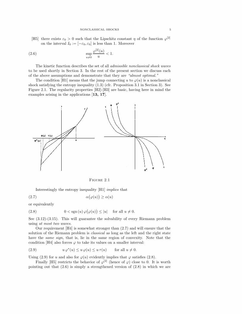
The condition [H1] means that the jump connecting u to ϕ(u) is a nonclassicalshock satisfying the entropy inequality (1.3) (cfr. Proposition 3.1 in Section 3). SeeFigure 2.1. The regularity properties [H2]-[H3] are basic, having here in mind theexamples arising in the applications [13, 17].
Figure 2.1
Interestingly the entropy inequality [H1] implies that
(2.7) α(ϕ(u)
)≥ α(u)
or equivalently
(2.8) 0 < sgn (u)ϕ(ϕ(u)
)≤ |u| for all u 6= 0.
See (3.12)-(3.15). This will guarantee the solvability of every Riemann problemusing at most two waves.
Our requirement [H4] is somewhat stronger than (2.7) and will ensure that thesolution of the Riemann problem is classical as long as the left and the right statehave the same sign, that is, lie in the same region of convexity. Note that thecondition [H4] also forces ϕ to take its values on a smaller interval:
(2.9) uϕ∗(u) ≤ uϕ(u) ≤ u τ(u) for all u 6= 0.
Using (2.9) for u and also for ϕ(u) evidently implies that ϕ satisfies (2.8).Finally [H5] restricts the behavior of ϕ[2] (hence of ϕ) close to 0. It is worth
pointing out that (2.6) is simply a strengthened version of (2.8) in which we are
5
6 P. BAITI, P. G. LEFLOCH AND B. PICCOLI
just excluding the case of equality. Moreover [H5] excludes only the case of equalityin d) of Lemma 2.1 below.
For concreteness, in the case where ϕ is smooth, then [H5] is equivalent tosaying ϕ′(0) > −1 and |ϕ[2](u)| < |u| for all u 6= 0. If ϕ is only Lipschitz continuous[H5] is indeed more general than these two conditions.
Let us derive some properties for the above functions near the inflection point.
Lemma 2.1. Under the assumptions (A1)-(A2) made on on the flux f , thefunctions τ and ϕ∗ satisfy
a) τ ′(0) ∈ (−1, 0).b) |τ(u)| < |u| for small u.
c)(ϕ∗)′(0) = −1.
d) If (2.8) holds and ϕ is differentiable at u = 0 then ϕ′(0) ∈ [−1, 1].
Proof. By hypothesis we have f(u) = Hu2p+1 + o(u2p+1). By the definition(2.1), τ = τ(u) satisfies(
H(2p+ 1)τ2p + o(τ2p))(u − τ) = Hu2p+1 + o(u2p+1)−Hτ2p+1 − o(τ2p+1).
By a bifurcation analysis it follows that τ is differentiable at u = 0. So, if weexpand τ(u) = Cu+ o(u), then it follows
Hu2p+1(
2pC2p+1 − (2p+ 1)C2p + 1)
+ o(u2p+1) = 0,
henceh(C) := 2pC2p+1 − (2p+ 1)C2p + 1 = 0.
By studying the zeroes of the function h, it follows that τ ′(0) = C ∈ (−1, 0). (Toillustrate this, note that for f(u) = u3 we have τ(u) = −u/2 and τ ′(0) = −1/2.)Hence a) holds as well as b).
By our hypotheses on the flux and the definition (2.3) of ϕ∗ it follows that
(2.10) Hu2p = H(ϕ∗(u)
)2p + o(u2p)
+ o((ϕ∗(u)
)2p).
Writing ϕ∗(u) = C′u+ o(u), (2.10) yields
Hu2p = H(C′u)2p + o(u2p),
hence (C′)2p = 1 which, together with uϕ∗(u) < 0, implies C′ = −1 and c) isproven.
Finally, assume that ϕ is differentiable so ϕ(u) = C′′ u+ o(u). In view of (2.8)
sgn (u)ϕ(ϕ(u)
)= (C′′)2 |u|+ o(u) ≤ |u|,
thus C′′ ∈ [−1, 1]. Hence d) follows. �
3. General Nonclassical Riemann Solver
A nonclassical Riemann solver is now defined from the kinetic function ϕ givenin Section 2. The classical entropy solutions (Oleinik [27], Liu [26]) are recoveredwith the trivial choice ϕ = τ . We also prove that our construction is essentially theunique possible one as long as the fundamental entropy inequality (1.3) is enforced(Assumption [H1]).
6
NONCLASSICAL SHOCKS 7
It is well-known that the Oleinik entropy criterion [27] states that a shockconnecting u− to u+ is (Oleinik)-admissible iff
(3.1)f(w)− f(u−)
w − u−≥ f(u+)− f(u−)
u+ − u−,
for all w between u− and u+. An easy consequence of (3.1) is that the chordconnecting the points
(u−, f(u−)
)and
(u+, f(u+)
)does not cross the graph of the
flux f .
Proposition 3.1. Consider the conservation law (1.1) in the class of weaksolutions satisfying the entropy inequality (1.3) for some strictly convex entropy U .
Then for every u there exists a point ϕ](u) such that a shock wave connectinga left state u− to a right state u+ satisfies the entropy inequality iff
(3.2) u− ϕ](u−) ≤ u− u+ ≤ u2
−.
Moreover we have
(3.3) u− τ−1(u−) < u− ϕ
](u−).
Proof. Let λ = λ(u−, u+) be the shock speed and consider the entropy dissi-pation
D(u−, u+) := −λ(U(u+)− U(u−)
)+ F (u+)− F (u−).
We easily calculate that
(3.4)
D(u−, u+) =∫ u+
u−
(f ′(m)− λ
)U ′(m) dm
= −∫ u+
u−
(f(m)− f(u−)− λ (m− u−)
)U ′′(m) dm.
The Rankine-Hugoniot relation for (1.1) yields λ:
λ =f(u+)− f(u−)
u+ − u−.
Suppose for definiteness that u− > 0. When u+ > u−, since f is convex in theregion m ∈ (u−, u+) we have
(3.5) f(m)− f(u−)− λ (m− u−) < 0
and therefore D(u−, u+) > 0. Moreover, it follows from (3.4) and the concav-ity/convexity properties of f , that the entropy dissipation u 7→ D(u−, u) achievesa minimum negative value at u = τ(u−) and vanishes at exactly two points (see anargument in [14]):
(3.6)
D(u−, ·) is monotone decreasing for u < τ(u−),D(u−, ·) is monotone increasing for u > τ(u−),
D(u−, τ(u−)
)< 0,
D(u−, u−) = 0,
D(u−, ϕ
](u−))
= 0.
Hence (3.2) follows. On the other hand when u+ ≤ τ−1(u−) it is geometrically clearthat the part of the graph of f corresponding to m ∈ (u+, u−) lies above the chord
7
8 P. BAITI, P. G. LEFLOCH AND B. PICCOLI
connecting the points (u−, f(u−)) and (u+, f(u+)). This means that the oppositesign holds now in (3.5). But since u+ < u− we again obtain that D(u−, u+) > 0.This implies that u− τ−1(u−) < u− ϕ
](u−). �
The shocks satisfying
(3.7) u− τ(u−) ≤ u− u+ ≤ u2−
are Oleinik-admissible and will be referred to as classical shocks. On the other handfor entropy admissible nonclassical shocks, (3.1) is violated, i.e.,
(3.8) u− ϕ](u−) ≤ u− u+ ≤ u− τ(u−).
This establishes that the condition [H1] in Section 2 is in fact a consequence of theentropy inequality (1.3).
From now on we rely on the kinetic function ϕ selected in Section 2 and wesolve the Riemann problem (1.1),
(3.9) u(x, 0) = u0(x) ={ul, for x < 0,ur, for x > 0,
where ul and ur are constants. We restrict attention to the case ul > 0, theother case being completely similar. To define the nonclassical Riemann solver wedistinguish between four cases:
(i) If ur ≥ ul, the solution u is a (Lipschitz continuous) rarefaction wave con-necting monotonically ul to ur.
(ii) If ur ∈[α(ul), ul
), the solution is a classical shock wave connecting ul to
ur.
(iii) If ur ∈(ϕ(ul), α(ul)
), the solution contains a (slower) nonclassical shock
connecting ul to ϕ(ul) followed by a (faster) classical shock connecting tour.
(iv) If ur ≤ ϕ(ul), the solution contains a nonclassical shock connecting ul toϕ(ul) followed by a rarefaction connecting to ur.
For ul = 0, the Riemann problem is a single rarefaction wave, connectingmonotonically ul to ur. The function u will be called the ϕ-admissible nonclassicalsolution of the Riemann problem. Clearly different choices for ϕ yield differentweak solutions u. This is natural as we already pointed out that limits given by(1.4) and similar models do depend on the parameter γ.
The above construction is essentially unique, as we show with the following twotheorems.
Theorem 3.2. Consider the Riemann problem (1.1)-(3.9) in the class of piece-wise smooth solutions satisfying the entropy inequality (1.3) for some strictly convexentropy U .
Then either the Riemann problem admits a unique solution or else there existsa one-parameter family of solutions containing at most two (shock or rarefaction)waves.
8
NONCLASSICAL SHOCKS 9
Next for any nonclassical shock connecting some states u− and u+ with thespeed λ, we impose the kinetic relation
(3.10) D(u−, u+) ={
Φ−(λ) if u+ < u−,
Φ+(λ) if u+ > u−,
where the kinetic functions are Lipschitz continuous and satisfy
(3.11)
Φ±(0) = 0,
Φ± is monotone decreasing,
Φ±(λ) ≥ D±(λ).
In the latter condition the lower bound D± is the maximum negative value of theentropy dissipation
D±(λ) := D(τ−1(u), u
), λ = f ′(u) for ± u ≥ 0.
Then (3.10) selects a unique nonclassical solution in the one-parameter familyof solutions.
Observe that given λ > 0 there are exactly one positive value and one negativevalue u such that λ = f ′(u). This property led us to define kinetic functions Φ±
for nonclassical shocks corresponding to decreasing and to increasing jumps.
Proof. The inequalities in Proposition 3.1 restrict the range of values takenby nonclassical shocks. First of all we show here that at most two waves can becombined together.
We now claim that
(3.12) ϕ](ϕ](u−)
)= u− for all u−.
Indeed we have by definition
D(u−, ϕ
](u−))
= 0, u− 6= ϕ](u−)
andD(ϕ](u−), ϕ]
(ϕ](u−)
))= 0, ϕ](u−) 6= ϕ]
(ϕ](u−)
).
The conclusion follows immediately from the fact that the entropy dissipation hasa single “nontrivial” zero; see (3.6).
We want to prove that the function u 7→ ϕ](u) is decreasing. Again, by abifurcation argument it follows that ϕ] is differentiable. Now notice that D(u, v) =−D(v, u) hence
(3.13) ∂uD(u−, ϕ
](u−))
= −∂vD(ϕ](u−), u−
).
From (3.6) we have that sgn(∂vD
(ϕ](u−), u−
))= −sgn
(∂vD
(u−, ϕ
](u−)))
, henceit follows that
(3.14) sgn(∂uD
(u−, ϕ
](u−)))
= sgn(∂vD
(u−, ϕ
](u−))).
Taking the total differential of the identity D(u−, ϕ
](u−))
= 0 with respect to u−and using (3.14) gives dϕ]/du− < 0 for all u−.
Consider a nonclassical shock connecting u− to ϕ(u−). By hypothesis u−ϕ](u−)≤ u−ϕ(u−) hence by the monotonicity of ϕ] and (3.12) it follows that u−ϕ]
(ϕ(u−)
)≤ u−ϕ
](ϕ](u−)
)= (u−)2. This prevents us to combine together more than two
9
10 P. BAITI, P. G. LEFLOCH AND B. PICCOLI
waves. Indeed since the speeds of the (rarefaction or shock) must be ordered (in-creasing) along a combination of waves, it is easily checked geometrically that theonly possible wave patterns are:
1. a rarefaction wave,2. a classical shock wave,3. a nonclassical shock followed by a classical shock,4. or else a nonclassical shock followed by a rarefaction.Finally we discuss the selection of nonclassical shocks. It is enough to prove that
for each fixed u− there is a unique nonclassical connection to a state u+ satisfyingboth the jump relation and the kinetic relation.
Suppose u− > 0 is fixed and regard the entropy dissipation as a function of thespeed λ:
Ψ(λ) = D(u−, u+(λ)
), λ =
f(u+(λ)
)− f(u−)
u+(λ) − u−.
It is not hard to see that
Ψ is increasing for λ ∈[f ′(τ(u−)), f ′(u−)
],
Ψ(f ′(τ(u−))
)= D+
(f ′(τ(u−))
)≤ Φ
(f ′(τ(u−))
),
Ψ(f ′(u−)
)= 0 ≥ Φ
(f ′(u−)
).
In view of the assumptions made on Ψ it is clear that the equation
Ψ(λ) = Φ(λ)
admits exactly one solution. This completes the proof that the nonclassical waveis unique. �
The property (3.12) implies that
(3.15) 0 < sgn (u)ϕ(ϕ(u)
)≤ |u| for all u 6= 0,
which is (2.8).
We have already seen that a kinetic relation is sufficient to select a unique wayof solving the Riemann Problem and the solution was described earlier. Now wewant to prove that this is essentially the unique expression a Riemann Solver canhave.
More precisely, assume the following are given:
• a set A of admissible waves satisfying the entropy inequality (1.3) for a fixed,strictly convex pair (U,F );• for every pair of states (ul, ur), a way of solving the associated Riemann prob-
lem, using only admissible waves in A. Denote by R(ul, ur) the Riemannsolution;
• an L1-continuous semigroup of solution for (1.1)-(1.2), compatible with theabove Riemann solutions. (Note that in [5] it is proven that, if such a semigroupexists, then there is a unique way of solving the Riemann problem associatedwith any pair of states ul, ur.)
Any collection of {R(ul, ur);ul, ur ∈ RI } satisfying the above assumptions will becalled here a basic A-admissible Riemann Solver. We are going to prove that
10
NONCLASSICAL SHOCKS 11
R(ul, ur) coincides with (i)-(iv) for some choice of the function ϕ. This completelyjustifies our study of the Nonclassical Riemann Solver made in the present paper.
The admissibility criterion imposed by A could be recovered by the analysis ofthe limits of some regularizations of (1.1) like (1.4), or by a kinetic relation as inthis paper (see also [13,14]). But it could also be given a priori by some physicalor mathematical argument.
Theorem 3.3. Every basic A-admissible Riemann Solver coincides with aNonclassical Riemann Solver for a suitable choice of the function ϕ.
Proof. In the previous discussion it was observed that there are only fourpossible wave patterns, namely a single shock, a single rarefaction wave or elsea nonclassical shock followed by either a shock or a rarefaction. Without loss ofgenerality, assume ul > 0. Any state ur > ul can be connected to the right of ulonly by a rarefaction wave, hence R(ul, ur) must coincide with this rarefaction.
In the following we shall consider all the shocks connecting ul to τ(ul) to benonclassical. Since ul can be connected by a single classical wave only to pointsur > τ(ul), then ul must be connected by a nonclassical shock to at least one rightstate ur ≤ τ(ul).
Let us see that this right point is unique. By contradiction, assume there existpoints u < u < 0 such that ul can be connected to both of them by a nonclassicalshock. By hypothesis u and u are connected by an (admissible) rarefaction. Hencethe Riemann problem (ul, u) can be solved either by a single nonclassical shock orby a nonclassical shock to u followed by a rarefaction to u. This contradicts theuniqueness of the Riemann solver R(ul, ur). It follows that ul can be connectedwith a nonclassical shock to exactly one right state, call it ϕ(ul).
By uniqueness, this implies immediately that all the states ur < ϕ(ul) are con-nected to the right of ul by the nonclassical shock to ϕ(ul) followed by a rarefactionto ur.
Introduce now the point α(ul) as in (2.5). The points in the interval [α(ul), ul)can not be reached neither by a rarefaction, nor by a wave pattern containing a(single) nonclassical shock. Hence they must be reached by a classical shock. Now,if ϕ(ul) = α(ul) = τ(ul) then we are done and the Riemann solution R(ul, ur)coincides with the Liu solution. Otherwise ϕ(ul) < τ(ul) < α(ul) and the pointsur in the interval
[ϕ(ul), τ(ul)
)are reached by the nonclassical shock followed by
a classical shock, since this is the only way to connect ul and ur. It remains tocover
[τ(ul), α(ul)
). The points in this interval can be reached either by a single
classical shock or by the nonclassical shock followed by a classical one. So, letul := sup{ur ≥ ϕ(ul) that are connected to the left of ul by the nonclassical shockfollowed by a classical one }. Then ul ≤ α(ul) and every u > ul is connected to leftof ul by a single classical shock. By the L1-continuity property and an analysis ofthe wave-speeds it follows that the solution of the Riemann problem (ul, ul) with anonclassical shock followed by a classical shock and the one with a single classicalshock must coincide, hence ul = α(ul). It follows that R(ul, ur) coincides with thenonclassical Riemann solver for this choice of ϕ. �
4. New Total Variation Functional
A classical way to prove convergence of approximate schemes for conservationlaws is to give uniform bounds on the L∞ and BV norms of the approximate
11

12 P. BAITI, P. G. LEFLOCH AND B. PICCOLI
solutions and then pass to the limit by using Helly’s compactness theorem. Un-fortunately, in contrast to the classical case, the total variation of the approximatesolutions can increase across interactions due to the creation or interaction of non-classical shocks. Hence a careful analysis is needed, of how the strengths of waveschange across interactions. In the classical case of systems [12] the so-called inter-action potential Q is used to compensate a (possible) increase of the total variation.In our case, however, it appears that if two fronts of strength σ and σ′ interact attime t (here strength means the size of the jump in the discontinuity) then thereare cases in which the variation of the total variation is linear in the strength ofthe incoming waves, i.e. ∆TV(t) ∼ C
(|σ|+ |σ′|
). This implies that we cannot use
the potential Q to control the increase in the total variation since Q is a quadraticfunctional (see [12]).
Our approach is to construct a modified total variation functional which de-creases in time along suitable wave-front tracking approximations of (1.1)-(1.2), andwhich is equivalent to the usual total variation, i.e. we are looking for a functionalV such that for every piecewise constant approximate solution v(t, x) constructedby front-tracking we have ∆V
(v(t, ·)
)≤ 0 for every t > 0 and there exist positive
constants C1, C2, depending only on the L∞ and BV norms of the initial datau0, such that C1 V(v) ≤ TV(v) ≤ C2 V(v) (see [3]). The definition of V can beregarded as a generalization of the standard distance |ur − ul|.
Now, let u : RI 7→ RI be a piecewise constant function and let xα, α = 1, . . . , N ,be the points of discontinuity of u. Define
(4.1) V(u) :=N∑α=1
σ(u(xα−), u(xα+)
),
where σ(ul, ur) measures the strength of the wave connecting the left state ul tothe right state ur. Notice that if σ(ul, ur) = |ur − ul|, then V(u) = TV(u). So, anew definition of the strength σ(ul, ur) is necessary. More precisely, we set(4.2)
σ(ul, ur) :={ (
ψ(ur)− ψ(ul))
sgn (ur − ul) sgn (ul) if(ur − ϕ(ul)
)sgn (ul) ≥ 0,
ψ(ur) + ψ(ul)− 2ψ(ϕ(ul)
)if(ur − ϕ(ul)
)sgn (ul) ≤ 0.
where ψ : RI 7→ RI is a continuous function that is increasing (resp. decreasing) foru positive (resp. negative). It is also assumed that ψ(0) = 0.
The wave strength σ depends on the kinetic function ϕ as well as on the functionψ to be determined in Section 5. Observe that the function ur 7→ σ(ul, ur) is apiecewise linear function in term of ψ(ur) resembling the letter W. It achieves alocal minimum value at ur = ul and at ur = ϕ(ul), the latter corresponding ofcourse to the nonclassical shock. Therefore the strength of the nonclassical shock iscounted less than what it would be with the standard total variation. This choiceis made to compensate for the increase of the standard total variation that arisesin certain wave interactions involving nonclassical shocks.
Let uν be the sequence of piecewise constant solutions of (1.1)-(1.2) constructedvia wave-front tracking from an approximation of the initial data u0, following [3].We replace the data u0 with a piecewise constant approximation uν(0) such that
(4.3) uν(0)→ u0 in the L1 norm, TV(uν(0))→ TV(u0).
12

NONCLASSICAL SHOCKS 13
Based on the nonclassical Riemann solver of Section 3, we approximately solvethe corresponding Cauchy problem for small time. Let δν be a sequence of positivenumbers converging to zero. For each ν, the approximate solution uν is constructedas follows. Solve approximatively the Riemann problem at each discontinuity pointof uν . This is obtained by approximating the solution given by the nonclassical Rie-mann solver: every shock or nonclassical shock travels with the correct shock speed,while the rarefaction fans are approximated by rarefaction fronts. More precisely,every rarefaction wave connecting the states ul and ur, say, with σ(ul, ur) > δν isapproximated by a finite number of small jumps traveling with speed equal to theright characteristic speed and with strength less than or equal to δν .
When two wave-front meet, we again use the nonclassical approximate Riemannsolver and continue inductively in time. The main aim is to estimate the totalvariation, that is to prove that there exists a positive constant C such that
(4.4) TV(uν(t)
)≤ C, t ≥ 0
uniformly in ν.From now on we assume that a kinetic function satisfying [H1]-[H5] is fixed.
First of all notice that under these hypotheses the interaction patterns for all couplesof waves are analogous to those considered and listed in Section 2 of [3]. We shallrely on this classification in the rest of the present section. To prove that uν iswell-defined, it is sufficient to show that the above construction can be carried onfor all positive times.
Proposition 4.1. Assume that the function
u 7→ sgn (u)(ψ(u)− ψ
(ϕ(u)
))is monotone increasing. Then the approximate solutions uν(t) are well-defined forall times t ≥ 0 and satisfy
(4.5) ‖uν(t)‖L∞(RI ) ≤ max{c, |ϕ(c)|
}, c := ‖uν(0)‖L∞(RI ).
Proof. As in [3] it is sufficient to prove that the total number of waves doesnot increase in time, so it can be bounded uniformly in t (for fixed ν). Since onlytwo waves may leave after the interaction of two waves, it is sufficient to prove thatthe rarefactions do not increase their strength across interaction. Denote by σ thestrength of rarefactions and ∆σ the change across the interaction. Referring to thecases of wave interactions listed in [3], we have (recalling that we assume ul > 0):
Case 1. Trivial case: ∆σ < 0.
Case 4. The variation of the strength across the interaction is computed by
∆σ =(ψ(ur)− ψ
(ϕ(ul)
))−(ψ(um)− ψ(ul)
)≤ ψ
(ϕ(um)
)− ψ(um)−
(ψ(ϕ(ul)
)− ψ(ul)
)≤ 0.
Case 6. This is a limiting case of Case 4.
∆σ = ψ(ϕ(um)
)− ψ(um)− ψ
(ϕ(ul)
)+ ψ(ul) ≤ 0.
Case 17. Now the variation is given by
∆σ =(ψ(ϕ(ul)
)− ψ(ur)
)−(ψ(um)− ψ(ur)
)< 0.
13
14 P. BAITI, P. G. LEFLOCH AND B. PICCOLI
So the approximate solutions are well-defined for all positive times.We now prove (4.5). It is obvious that the only interactions that can increase
the L∞-norm are those in which a nonclassical shock is involved. Let R(u) be therange of a piecewise constant function u. For every approximate solution uν , acrossan interaction at time t we have
(4.6) R(uν(t+, ·)
)⊆ R
(uν(t−, ·)
)∪R
(ϕ(uν(t−, ·)
)),
as follows from the definition of the Riemann solver in Section 3. It is clear that(4.5) holds for t = 0+. Now fix ν and assume that for a positive time t we have
M(t) := ‖uν(t, ·)‖L∞ > ‖uν(0, ·)‖L∞ .
Then by (4.6), there exists u ∈ R(uν(0, ·)
)and a positive integer n such that
M(t) =∣∣ϕ[n](u)
∣∣.Recall that
∣∣ϕ[2](u)∣∣ ≤ |u|. Hence n must be odd, otherwise by induction
M(t) =∣∣ϕ[n](u)
∣∣ ≤ |u| ≤ ‖uν(0, ·)‖L∞ ,
which is a contradiction. So n = 2q + 1 and again by induction it follows that
M(t) =∣∣ϕ[2q]
(ϕ(u)
)∣∣ ≤ ∣∣ϕ(u)∣∣ ≤ ∣∣ϕ(‖uν(0, ·)‖L∞
)∣∣.Hence (4.5) follows. This completes the proof of Proposition 4.1. �
Assuming now that the approximate initial data satisfy
(4.7) ‖uν(0)‖L∞(RI ) ≤ C ‖u0‖L∞(RI ),
we conclude from (4.5) that
(4.8) ‖uν(t)‖L∞(RI ) ≤ C′ for all t ≥ 0,
uniformly in ν.
We next derive a uniform BV bound or, more precisely, we prove that Vdecreases along approximate solutions.
Proposition 4.2. Assume that the function
(4.9) u 7→ sgn (u)(ψ(u)− ψ
(ϕ(u)
))is monotone increasing.
Then for the approximate solutions,
(4.10) t 7→ V(uν(t)
)is monotone decreasing.
14
NONCLASSICAL SHOCKS 15
Proof. The function t 7→ V(uν(t)
)is piecewise constant with discontinuities
located only at interaction times. Hence it suffices to show that V decreases acrossevery collision. Assume that the three states ul, um and ur, are separated bytwo interacting wave fronts of strength σ−1 and σ−2 , each being generated by a(nonclassical) Riemann solution. Each front can be either a classical, nonclassicalshock or a rarefaction wave.
The complete list of interaction patterns can be found in Section 2 of [3], butCases 5 and 12 therein never occur because of our assumption [H2]. In [3] a caseby case analysis was developed. Here thanks to the general definition (4.1)-(4.2)we have some simplifications.
Any outgoing pattern is made of at most two waves, with strength σ+1 and
(possibly) σ+2 . Hence the variation of V across the interaction is given by ∆V =
(σ+1 + σ+
2 )− (σ−1 + σ−2 ) := Σ+ − Σ−.The function σ introduced in (4.2) satisfies the following key properties:
(i) σ is additive on ordered waves, in the sense that if u1, u2, u3 are three statessuch that u1 < u2 < u3 and such that sgn (ui)
(uj −ϕ(ui)
)≥ 0 for all i > j,
thenσ(u1, u3) = σ(u1, u2) + σ(u2, u3),σ(u3, u1) = σ(u3, u2) + σ(u2, u1);
(ii) if sgn (u1) = sgn (u2) then σ(u1, u2) = σ(u2, u1);
(iii) for every outgoing pattern we have Σ+ = σ(ul, ur).
These properties can be checked from the definition of σ. In particular (iii) impliesthat ∆V ≤ 0 iff Σ− ≥ σ(ul, ur).
The interaction cases can be split in four families.
Cases 8, 9, 10, 11, 15, 16, 17. The states before the interaction are ordered.Hence by (i) it follows that Σ− = σ(ul, ur) and so ∆V = 0.
Cases 1, 2, 3, 4, 7. The states before the interaction are not ordered. Then acancellation takes place, but the canceled wave lives on one region of convexity.Using (i)-(ii) it follows that Σ− > σ(ul, ur), hence ∆V < 0.
Cases 13, 14, 18, 19. As in the previous case but now the canceled wave crossthe state 0. Indeed all of them are special cases of 14. For the latter, it easy to seethat Σ+ = ψ(ul) − ψ(ur) and Σ− =
(ψ(ul) − ψ(um)
)−(ψ(um) − ψ(ur)
), hence
∆V = 0.
It remains to check only Case 6.Case 6. This is the only case which requires condition (4.9). Indeed, ul(ul−um) >0 and it follows that
∆V = ψ(ul)− ψ(ϕ(ul)
)+ ψ
(ϕ(um)
)− ψ
(ϕ(ul)
)+
−(ψ(um)− ψ(ul)
)−(ψ(um)− ψ
(ϕ(um)
))= 2[(ψ(ul)− ψ
(ϕ(ul)
))−(ψ(um)− ψ
(ϕ(um)
))]≤ 0.
This completes the proof. �
The existence of a function ψ satisfying the condition (4.9) will be establishedin Section 5. The equivalence between TV and V will be proved there, too. Nowwe are ready to conclude with the main result of the present paper.
15
16 P. BAITI, P. G. LEFLOCH AND B. PICCOLI
Theorem 4.3. Consider the conservation law (1.1) together with the nonclas-sical Riemann solver characterized by the function ϕ : RI → RI . Suppose that ϕsatisfies the assumptions [H1]–[H5] listed in Section 2.
Given an initial data u0 with bounded total variation, there exists a positiveconstant C depending only on ϕ and the L∞-norm of u0 such that the approximatesolutions uν(t) (constructed by wave-front tracking) satisfy
(4.11) TV(uν(t)
)≤ C TV(u0)
for all times t ≥ 0.A subsequence of uν converges in the L1 norm toward a weak solution of the
conservation law (1.1)-(1.2) which satisfies the entropy inequality (1.3).
Proof. By (4.8)-(4.10), the approximate solutions constructed above haveuniformly bounded L∞-norm and total variation. We can apply Helly’s theorem tofind a (sub)sequence which converges in L1
loc to a function u. Since the modifiedand the usual strengths of waves are equivalent (see (5.10)) u is a nonclassical weaksolution of (1.1)-(1.2) satisfying also the entropy inequality (1.3). �
5. Construction of the Function ψ
In this section we prove the existence of a function ψ satisfying (4.9) needed inPropositions 4.1 and 4.2. This will be accomplished by a fixed-point argument ina suitable function space X defined below.
Denote by LipI(ψ) the Lipschitz constant of a function ψ defined on someinterval I. Let M > 0 be a constant greater than the L∞-norm of u0 and defineJM := [−M,M ] ∪
[ϕ(M), ϕ(−M)
]. Finally, let LM be the Lipschitz constant of ϕ
in the set JM . Introduce the space
X :={ψ ∈ C
(JM ;RI
): ψ(0) = 0, ‖ψ‖
X<∞
},
endowed with the norm
‖ψ‖X
:= supu6=0
∣∣∣∣ ψ(u)u− ϕ(u)
∣∣∣∣ .Then define the subset Y ⊂ X by
Y :={ψ ∈ X : ψ is
increasingdecreasing for u ≷ 0; LipI0(ψ) ≤ K
},
where K ≥ (1 + LM )/(1 − η) is a fixed constant and η is the Lipschitz constantintroduced in [H5].
The reason why we consider JM instead of [−M,M ] is that we need a ϕ-invariant set and actually ϕ(JM ) ⊆ JM while in general this is not true for [−M,M ].
Lemma 5.1.
(X, ‖ · ‖
X
)is a Banach space and Y is a closed subset.
Proof. It is clear that X is a normed space. Let us see that it is complete.Let ψn ∈ X , n = 1, 2, . . . be a Cauchy sequence in the norm ‖ · ‖X . By definition,for every ε > 0, there exists n such that for all m,n ≥ n we have
(5.1)∣∣ψn(u)− ψm(u)
∣∣ ≤ |u− ϕ(u)| ε
16
NONCLASSICAL SHOCKS 17
for all u 6= 0, but also for u = 0. Hence the sequence ψn is also Cauchy in thespace C
(JM ;RI
)with the sup-norm, and so it converges to a continuous function
ψ. Moreover, by passing pointwise to the limit, we see that ψ(0) = 0. Finally byletting m→∞ in (5.1) we see that the convergence holds actually in the space X .
Finally let us see that Y is closed. Take ψn → ψ in X with ψn ∈ Y for alln. First of all, by passing pointwise to the limit, it follows that ψ satisfies themonotonicity properties. By hypothesis we have
(5.2)∣∣∣∣ψn(u)− ψn(v)
u− v
∣∣∣∣ ≤ Kfor all n and all u, v ∈ I0 with u 6= v. Since ψn converges to ψ pointwise, by passingto the limit in (5.2) we get LipI0(ψ) ≤ K, hence ψ ∈ Y and Y is closed. �
Now define the map T : X 7→ X by the relation
(5.3)(Tψ)(u) := ψ
(ϕ(u)
)+ |u|, u ∈ RI .
Theorem 5.2. T maps X into X and is a contraction.
Proof. Let ψ ∈ X be fixed. It is clear that(Tψ)(0) = 0. Let us see that T is
a contraction. For all ψ, ψ ∈ X and u 6= 0 we have∣∣∣∣Tψ(u)− T ψ(u)u− ϕ(u)
∣∣∣∣ =
∣∣∣∣∣ϕ(u)− ϕ(ϕ(u)
)u− ϕ(u)
∣∣∣∣∣∣∣∣∣∣ψ(ϕ(u)
)− ψ
(ϕ(u)
)ϕ(u)− ϕ
(ϕ(u)
) ∣∣∣∣∣ ,hence ∥∥Tψ − T ψ∥∥
X≤ sup
u6=0
∣∣∣∣∣ϕ(u)− ϕ(ϕ(u)
)u− ϕ(u)
∣∣∣∣∣ · ∥∥ψ − ψ∥∥X ,and by taking ψ ≡ 0 in this last inequality, it follows that ‖Tψ‖
X<∞ and T maps
X into itself. Now, it is easy to see (i.e. geometrically) that
(5.4)
∣∣∣∣∣ϕ(u)− ϕ(ϕ(u)
)u− ϕ(u)
∣∣∣∣∣ < 1, u 6= 0,
or even more
(5.5)
∣∣∣∣∣ϕ(u)− ϕ(ϕ(u)
)u− ϕ(u)
∣∣∣∣∣ =ϕ(ϕ(u)
)− ϕ(u)
u− ϕ(u)= 1−
1− ϕ(ϕ(u)
)/u
1− ϕ(u)/u,
for all u 6= 0. By (2.6) and (5.5) it follows that
supu6=0
∣∣∣∣∣ϕ(u)− ϕ(ϕ(u)
)u− ϕ(u)
∣∣∣∣∣ < 1.
Hence T is a contraction. �
By the contraction principle the map T has a unique fixed point in X . Denoteit by ψ : JM → RI . By construction the function ψ(u) − ψ
(ϕ(u)
)is monotone in-
creasing (resp. monotone decreasing) for u positive (resp. negative). More preciselyin view of (5.3) and T (ψ) = ψ, we have
(5.6)ψ(u)− ψ
(ϕ(u)
)= u, for u > 0,
ψ(u)− ψ(ϕ(u)
)= −u, for u < 0.
17
18 P. BAITI, P. G. LEFLOCH AND B. PICCOLI
Therefore the assumption of Propositions 4.1 and 4.2 holds together with the uni-form L∞ bound (4.8) and the bound for the new functional V
(uν(t)
), i.e. (4.10).
At this point it seemed we could not say anything about the regularity of ψclose to 0. And we will need ψ to be Lipschitz continuous on I0 to prove equivalencebetween TV and V.
Let us consider the second iterate of T : X 7→ X .
Lemma 5.3. T [2] : X 7→ X and is a contraction. Moreover T [2] maps Y intoitself.
Proof. The first assertion is trivial. Take ψ0 ∈ Y . By our definition and [H2]it follows that T [2]ψ is increasing (resp. decreasing) for u positive (resp. negative).Iterating (5.3), we get that T [2] is defined by
(5.7) T [2]ψ(u) = ψ(ϕ[2](u)
)+ sgn (u)
(u− ϕ(u)
), u ∈ RI .
The relation (5.7) together with ϕ[2](I0)⊂ I0, imply
(5.8) LipI0(T [2]ψ0
)≤ 1+LipI0(ϕ)+Lipϕ[2](I0)(ψ0)·LipI0
(ϕ[2])≤ 1+LM+Kη ≤ K,
by the choice of K. Hence T [2]ψ0 ∈ Y . �
Now, T [2] is a contraction on X , hence it admits a unique fixed point. SinceT [2] maps Y into Y and Y is closed, it follows that this fixed point belongs to Y .Every fixed point of T is also a fixed point of T [2], hence T [2] and T have the samefixed point. Thus the fixed point of T belongs to Y and so it is Lipschitz continuouson a neighborhood of 0 and satisfies the monotonicity properties.
Remark 5.4. The operator T does not map Y into Y . Nevertheless, sinceT [2] maps Y into Y and ϕ is Lipschitz, it follows that, for every ψ ∈ X , also theLipschitz constant of T [2n+1]ψ cannot grow too much as n→∞.
We point out that if ψ0 were a fixed point of T [2] only, then we could not recoverthe relations (5.6). So we need ψ to be a fixed point of both T and T [2].
Finally we prove that the functional V is equivalent to the usual total variation.
Lemma 5.5. Given M > 0, there exist positive constants C1, C2 such that
(5.9) C1 V(u) ≤ TV(u) ≤ C2 V(u)
for any piecewise constant function u with ‖u‖L∞ ≤M .
Proof. It is sufficient to prove that
(5.10) C1 σ(ul, ur) ≤ |ur − ul| ≤ C2 σ(ul, ur),
for all ul, ur with |ul|, |ur| ≤ M . Without loss of generality we can assume ul > 0.For all ur > 0, by the monotonicity of ψ and ϕ we have∣∣ψ(ur)− ψ(ul)
∣∣ =∣∣ψ(ϕ(ur)
)− ψ
(ϕ(ul)
)∣∣+ |ur − ul| ≥ |ur − ul|,
hence
(5.11)∣∣∣∣ ur − ulσ(ul, ur)
∣∣∣∣ =∣∣∣∣ ur − ulψ(ur)− ψ(ul)
∣∣∣∣ ≤ 1.
18

NONCLASSICAL SHOCKS 19
If, instead, ur < 0 we have
(5.12)∣∣∣∣ ur − ulσ(ul, ur)
∣∣∣∣ ≤∣∣∣∣∣ ul − ϕ(ul)ψ(ul)− ψ
(ϕ(ul)
) ∣∣∣∣∣ =∣∣∣∣ul − ϕ(ul)
ul
∣∣∣∣ ≤ (1 + LM ) =: C2,
since |ϕ(u)| ≤ LM |u| for all |u| ≤M .Next we prove that ψ is Lipschitz continuous on I := [−M,M ] (hence also on
JM ). First of all, we can assume M > ε0. Since ψ is a fixed point of T [2] it followsthat
ψ(u) = ψ(ϕ[2](u)
)+ sgn (u)
(u− ϕ(u)
),
which implies
(5.13) LipI(ψ) ≤ LipI(ϕ[2])· Lipϕ[2](I)(ψ) + LipI(ϕ) + 1.
Note that by (5.13) the Lipschitz constant of ψ on the interval [−M,M ] can becontrolled by that on the (strictly) smaller interval
[ϕ[2](−M), ϕ[2](M)
].
More precisely, even though LipI(ϕ[2]) may be greater than 1, it happens that
the function ϕ[2] has only one fixed point on (−∞,+∞), namely u = 0. Hence,having fixed M > ε0, there exists an integer p such that the iterates ϕ[2p](u) ∈[−ε0, ε0] for all |u| ∈ [ε0,M ], where p depends only on ε0 and M . By iterating(5.13), this implies that
(5.14) LipI(ψ) ≤ K1 · LipI0(ψ) +K2,
where K1,K2 are constants depending only on M, ε0 and the Lipschitz constant ofϕ. Since LipI0(ψ) ≤ K, (5.14) says that ψ is Lipschitzian.
Then the conclusion holds with
C1 :=(K1 · LipI0(ψ) +K2
)−1
.
�
6. Remarks on the Construction
The present result is stronger than the one presented in [3]. On one hand weconsider a more general flux-function; moreover we drop both the assumption thatthe solution should coincide with the classical one in a small neighborhood of 0(see (H2) in [3]), and the assumption that α should be decreasing. Concerning thislast hypothesis, notice that in the cubic-flux case with the choice ψ(u) = |u| (as weconsidered in [3]) we have
sgn (u)(ψ(u)− ψ
(ϕ(u)
))= −α(u).
So, α is decreasing iff (4.9) holds. This means that the monotonicity request on αcomes out by the particular choice ψ(u) = |u|. The assumption can be drop justby carefully choosing the function ψ.
The choice (4.2) appears to be a sort of nonlinear generalization of the def-inition of σ(ul, ur) given in [3], the latter corresponding to the case ψ(u) = |u|.Unfortunately this last choice does not work in the general case mainly because theflux-function f is not symmetric.
19
20 P. BAITI, P. G. LEFLOCH AND B. PICCOLI
The case ϕ ≡ τ corresponds to the classical case in which the Oleinik-Liusolutions [26,27] are selected. Notice that in view of Lemma 2.1 hypotheses [H1]-[H5] are automatically satisfied. So, we expects that a sufficient condition for thenonclassical solution to be in BV is that ϕ and τ have the same behavior nearu = 0, roughly speaking ϕ′(0) = τ ′(0). In fact, we could prove existence in BVunder the weaker hypothesis [H5].
The function |u| on the right-hand side of (5.3) can be replaced by a more gen-eral Lipschitz continuous function G(u), i.e. we can look for a function ψ satisfyingthe equation
ψ(u) = ψ(ϕ(u)
)+G(u),
with G increasing (resp. decreasing) for u positive (resp. negative), and behavinglike |u| for u close to 0. The corresponding function ψ obtained by a fixed-pointargument similar to the one presented in the previous section, depends on G and,in general, is nonlinear. Indeed, if one tries to use a piecewise linear ψ of the form
(6.1) ψ(u) :={λ+u, for u > 0,λ−u, for u < 0,
for some positive λ+ and negative λ−, then the condition σ ≥ 0 (more preciselysgn (u)
(ψ(u)− ψ
(ϕ(u)
))≥ 0) implies that m := λ−/λ+ must satisfy
supv<0
∣∣∣∣ϕ(v)v
∣∣∣∣ =: A− ≤ |m| ≤ A+ := infu>0
∣∣∣∣ u
ϕ(u)
∣∣∣∣ .So a necessary condition is A− ≤ A+. If ϕ(u) = −αu + o(u), then the previouscondition is violated as long as there exists a state w such that |ϕ(w)| > α−1|w|,and this could be the case when the flux is not symmetric. Nevertheless the choice(6.1) works for (1.1) with a symmetric flux function, and in this case one can takeλ+ = −λ− = 1, provided that ϕ′(u) > −1 for all u.
If we are interested only in small data it is possible to choose ψ(u) = |u| evenfor general fluxes and regular ϕ. Indeed, if ϕ ∈ C1 and ϕ′(0) > −1, then (5.6)reduces to [
sgn(u)(ψ − ψ(ϕ))]′(u) =
(1 + ϕ′(u)
),
which is positive for u close to zero.Finally, our hypothesis [H5] seems to be unavoidable, as there are counterex-
amples (see Section 7) in which ϕ′(0) = −1 and the total variation of the solutionblows up in finite time.
7. Examples of Blow-Up of the Total Variation
In this section we present two examples in which hypothesis [H5] does not holdand the total variation of the exact nonclassical solution blows up in finite time.For a recent important result about blow-up for systems of conservation laws, seeJenssen [19].
Example 7.1. Consider the equation (1.1) with the following flux-function
f(u) :={uh, u ≥ 0,uk, u < 0,
with k > h odd and greater than 1. It should be stressed that this function doesnot satisfy our regularity conditions since it is only Lipschitz continuous at the
20
NONCLASSICAL SHOCKS 21
origin. Nevertheless, the example presented now is of interest since it shows newfeatures not encountered in the classical case. We recall that, when the classicalOleinik entropy condition is enforced, the solution of the Cauchy problem (1.1)-(1.2)with Lipschitz continuous flux has bounded variation and in fact is total variationdiminishing.
In the context of nonclassical solutions, we will produce an example where theinitial data is in BV but the total variation of the solution blows up instantaneouslyat t = 0. This actually happens for a particular choice of the kinetic function ϕ forwhich ϕ′(0+) = −∞. It should be noticed that also τ ′(0+) = −∞, nevertheless theclassical solution exists and is in BV. This means that in the case of a Lipschitzcontinuous flux-function, whether the total variation of the solution blows up ornot, is not determined by the value of ϕ′(0) but, as we shall see, can be related tothe behavior of the function α− ϕ near u = 0.
It is not difficult to see that for u positive ϕ∗(u) = −uγ, where γ = h−1k−1 < 1,
and that τ(u) < τk(u) where τk(u) satisfies (2.1) with f(u) = uk for all u. Henceτ(u) < −Cku for a positive constant Ck depending only on k, and so τ(u) < −2u2
if for example 0 < 2u < Ck. Choose now α(u) = −u2 > τ(u) for all u ≥ 0. Itfollows that ϕ(u) = −uγ
(1 +O(u)
), hence
α(u)− ϕ(u) ≥ −u2 +12uγ ,
if u is sufficiently small.Choose now an integer n0 such that 1/nβ0 < Ck where β = 1/γ > 1. Take the
initial data of the form
u0(x) :=
1/nβ0 , if x ∈ (−∞, 2n0],1/nβ, if x ∈ (2n, 2n+ 1), n ≥ n0,
−2/n2β, if x ∈(2n+ 1, 2(n+ 1)
), n ≥ n0.
An easy estimate implies that
TV(u0) ≤ 4∞∑
n=n0
1nβ
<∞.
For small positive t, the solution is obtained just by solving the Riemann problemsat each discontinuity point in u0. Notice that −2/n2β > τ(1/nβ), hence the Rie-mann problem with data (1/nβ,−2/n2β) is solved by a nonclassical shock from 1/nβ
to ϕ(1/nβ
)followed by a classical shock from ϕ
(1/nβ
)to −2/n2β. In particular it
follows that
∆TV(0) ≥∞∑
n=n0
(α(1/nβ)− ϕ(1/nβ)
)≥ 1
2
∞∑n=n0
1nγβ−∞∑
n=n0
1n2β≥ 1
2
∞∑n=n0
1n.
This implies that ∆TV(0) = +∞ hence TV(0+) = +∞.Finally, notice that u(t, ·) 6∈ BV but u(t, ·) ∈ BVloc.
21
22 P. BAITI, P. G. LEFLOCH AND B. PICCOLI
Example 7.2. Now we will take f(u) = u3, so our hypotheses on the flux-function are satisfied. Since the total variation of the solution of the Riemannproblem (ul, ur) depends in a Lipschitz continuous way on |ul−ur|, it appears thatin this case the total variation can not blow up instantaneously. In fact, we shallprove that for suitable initial data u0 and choice of the kinetic function ϕ, thereexists a time t such that
TV(u(t, ·)
)= +∞,
for all t ≥ t, where u is the solution of (1.1)-(1.2).We shall consider the case ϕ(u) = ϕ∗(u) = −u for all u, hence ϕ(u) does not
satisfy [H5]. In this situation every Riemann problem with ulur < 0 generatesa nonclassical shock; more precisely the solution is given by a nonclassical shockconnecting ul to −ul followed by a classical shock connecting −ul to ur, no matterhow small ur is. This means that arbitrarily small oscillations near 0 can producenonclassical shocks of arbitrarily large strength. For related results connected withthe study of radially symmetric systems, see the works of Freistuhler, for instancein [10, 11].
Now let us construct initial data for which the total variation of the solutionblows up. We define u0(x) to be equal to 1 for x < 0 and equal to 0 for 0 < x <x0 := 1. In x0 a rarefaction will originate. First of all, the Riemann problem inx = 0 is solved by a single classical shock traveling with speed λ0 := λ(1, 0) = 1.We want to define inductively points xn, yn and states un such that xn−1 < yn < xnfor all n and u0 is given by
(7.1) u0(x) :=
un, if xn−1 < x < yn,
0, if yn < x < xn,
0, if x > supn xn.
The idea is the following: start at x0 and take u1 small and negative to be definedlater. The Riemann problem at x0 is solved by a rarefaction wave which will interactwith the original shock outgoing from the origin, at the point P0 := (1, 1) in the(x, t)-plane. This interaction will produce a slower nonclassical shock connecting 1to −1 and a faster classical shock which will interact with the rarefaction until thepoint P1 (see Figure 7.1). Let x1 be the x-coordinate of point P1. Now, draw backthe line with slope λ(u1, 0) passing through P1. Let y1 be the x-coordinate of theintersection point between this line and the x-axis. Notice that 0 < λ(u1, 0) < λ(u1)hence we have x0 < y1 < x1. Moreover the Riemann problem at y1 is actually solvedby the shock traveling with speed λ(u1, 0). Since P1 depends only on the speed atthe right of the rarefaction (that is λ(u1) = 3u2
1), then it is clear that once u1 isknown, so x1, y1 are.
Let us now proceed inductively: assume points xn, yn and value un+1 are givenand assume that the rarefaction originating at xn interacts with the shock origi-nating at yn at the point Pn, producing a nonclassical shock connecting (−1)n to(−1)n+1 traveling with speed 1 and a classical shock interacting with the previousrarefaction until point Pn+1. As before let xn+1, yn+1 be the x-coordinates of thepoint Pn+1 and the intersection-point between the x-axis and the line with slopeλ(un+1) passing through Pn+1, respectively. Again xn < yn+1 < xn+1.
We notice that each interaction at Pn generates a nonclassical shock betweenthe states 1 and −1, traveling with speed 1. Hence these fronts will never interact
22
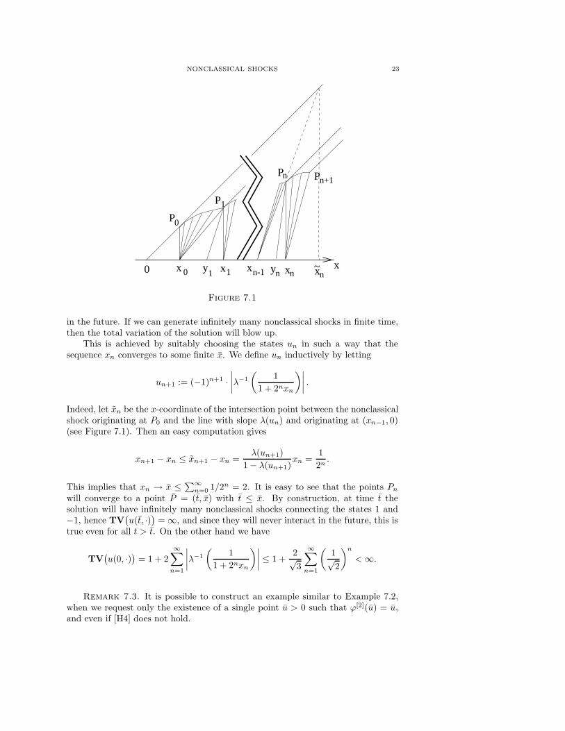
NONCLASSICAL SHOCKS 23
x 0 y1
P1
x1
P0
xn~xnyn
xn-1
Pn Pn+1
0 x
Figure 7.1
in the future. If we can generate infinitely many nonclassical shocks in finite time,then the total variation of the solution will blow up.
This is achieved by suitably choosing the states un in such a way that thesequence xn converges to some finite x. We define un inductively by letting
un+1 := (−1)n+1 ·∣∣∣∣λ−1
(1
1 + 2nxn
)∣∣∣∣ .Indeed, let xn be the x-coordinate of the intersection point between the nonclassicalshock originating at P0 and the line with slope λ(un) and originating at (xn−1, 0)(see Figure 7.1). Then an easy computation gives
xn+1 − xn ≤ xn+1 − xn =λ(un+1)
1− λ(un+1)xn =
12n.
This implies that xn → x ≤∑∞
n=0 1/2n = 2. It is easy to see that the points Pnwill converge to a point P = (t, x) with t ≤ x. By construction, at time t thesolution will have infinitely many nonclassical shocks connecting the states 1 and−1, hence TV
(u(t, ·)
)=∞, and since they will never interact in the future, this is
true even for all t > t. On the other hand we have
TV(u(0, ·)
)= 1 + 2
∞∑n=1
∣∣∣∣λ−1
(1
1 + 2nxn
)∣∣∣∣ ≤ 1 +2√3
∞∑n=1
(1√2
)n<∞.
Remark 7.3. It is possible to construct an example similar to Example 7.2,when we request only the existence of a single point u > 0 such that ϕ[2](u) = u,and even if [H4] does not hold.
23
24 P. BAITI, P. G. LEFLOCH AND B. PICCOLI
References
[1] R. Abeyaratne and J. Knowles, Kinetic relations and the propagation of phase boundaries insolids, Arch. Rational Mech. Anal. 114 (1991), 119–154.
[2] R. Abeyaratne and J. Knowles, Implications of viscosity and strain gradient effects for thekinetics of propagating phase boundaries in solids, SIAM J. Appl. Math. 51 (1991), 1205–1221.
[3] D. Amadori, P. Baiti, P.G. LeFloch and B. Piccoli, Nonclassical shocks and the Cauchyproblem for nonconvex conservation laws, J. Differential Equa. 151 (1999), 345–372.
[4] P. Baiti and H.K. Jenssen, On the front-tracking algorithm, J. Math. Anal. Appl. 217 (1998),395–404.
[5] P. Baiti, P.G. LeFloch and B. Piccoli, Uniqueness of classical and nonclassical solutions fornonlinear hyperbolic systems, preprint.
[6] P. Baiti, P.G. LeFloch and B. Piccoli, Nonclassical shocks and the Cauchy problem: Strictlyhyperbolic systems, in preparation.
[7] A. Bressan, Global solutions to systems of conservation laws by wave-front tracking, J. Math.Anal. Appl. 170 (1992), 414–432.
[8] C. Dafermos, Polygonal approximations of solutions of the initial value problem for a con-servation law, J. Math. Anal. Appl. 38 (1972), 33–41.
[9] R.J. DiPerna, Global existence of solutions to nonlinear hyperbolic systems of conservationlaws, J. Differential Equa. 20 (1976), 187–212.
[10] H. Freistuhler, Non-uniformity of vanishing viscosity approximation, Appl. Math. Lett. 6(1993), 35–41.
[11] H. Freistuhler, On the Cauchy problem for a class of hyperbolic systems of conservation laws,J. Differential Equa. 112 (1994), 170–178.
[12] J. Glimm, Solutions in the large for nonlinear hyperbolic systems of equations, Comm. PureAppl. Math. 18 (1965), 697–715.
[13] B.T. Hayes and P.G. LeFloch, Nonclassical shocks and kinetic relations: Scalar conservationlaws, Arch. Rational Mech. Anal. 139 (1997), 1–56.
[14] B.T. Hayes and P.G. LeFloch, Nonclassical shocks and kinetic relations: Strictly hyperbolicsystems, SIAM J. Math. Anal., to appear.
[15] B.T. Hayes and P.G. LeFloch, Nonclassical shocks and kinetic relations: Finite differenceschemes, SIAM J. Numer. Anal. 35 (1998), 2169–2194.
[16] B.T. Hayes and M. Shearer, Undercompressive shocks for scalar conservation laws with non-convex fluxes, Preprint, North Carolina State Univ., 1997.
[17] D. Jacobs, W.R. McKinney and M. Shearer, Traveling wave solutions of the modified Korteweg-deVries Burgers equation, J. Differential Equa. 116 (1995), 448–467.
[18] R.D. James, The propagation of phase boundaries in elastic bars, Arch. Rational Mech. Anal.73 (1980), 125–158.
[19] H.K. Jenssen, Blow-up for systems of conservation laws, Preprint, 1998.[20] S.N. Kruzkov, First order quasilinear equations in several independent variables, Math. USSR
Sbornik 10 (2) (1970), 217–243.[21] P.D. Lax, Hyperbolic systems of conservation laws II, Comm. Pure Appl. Math. 10 (1957),
537–566.[22] P.D. Lax, Shock waves and entropy, Contributions to Nonlinear Functional Analysis, ed. E.A.
Zarantonello, Academic Press, New York, 1971, pp. 603–634.[23] P.G. LeFloch, Propagating phase boundaries: formulation of the problem and existence via
the Glimm scheme, Arch. Rational Mech. Anal. 123 (1993), 153–197.[24] P.G. LeFloch, An introduction to nonclassical shocks of systems of conservation laws, Pro-
ceedings of the “International School on Theory and Numerics for Conservation Laws”,Freiburg/Littenweiler (Germany), 20–24 October 1997, ed. D. Kroner, M. Ohlberger andC. Rohde, Lecture Notes in Computational Science and Engineering (1998), pp. 28–72.
[25] P.G. LeFloch and C. Rohde, High-order schemes, entropy inequalities and nonclassical shocks,in preparation.
[26] T.P. Liu, Admissible solutions of hyperbolic conservation laws, Memoir Amer. Math. Soc.240, 1981.
[27] O. Oleinik, Discontinuous solutions of nonlinear differential equations, Usp. Mat. Nauk. 12(1957), 3–73 (in Russian); English transl. in Amer. Math. Soc. Transl. Ser. 2 (26), 95–172.
24
NONCLASSICAL SHOCKS 25
[28] N.H. Risebro, A front-tracking alternative to the random choice method, Proc. Amer. Math.Soc. 117 (1993), 1125–1139.
[29] M. Shearer, The Riemann problem for a class of conservation laws of mixed type, J. Differ-ential Equa. 46 (1982), 426–443.
[30] M. Slemrod, Admissibility criteria for propagating phase boundaries in a van der Waals fluid,Arch. Rational Mech. Anal. 81 (1983), 301–315.
[31] L. Truskinovsky, Dynamics of non-equilibrium phase boundaries in a heat conducting non-linear elastic medium, J. Appl. Math. Mech. (PMM) 51 (1987), 777–784.
[32] L. Truskinovsky, Kinks versus shocks, Shock induced transitions and phase structures ingeneral media, R. Fosdick, E. Dunn, and M. Slemrod ed., IMA Vol. Math. Appl. 52, Springer-Verlag, 1993.
[33] A.I. Volpert, The space BV and quasilinear equations, Math. USSR Sb. 2 (1967), 225–267.
Universita di Padova, Via G.B. Belzoni 7, 35131 Padova, Italy.
E-mail address: [email protected]
Centre de Mathematiques Appliquees & Centre National de la Recherche Scien-
tifique, U.M.R. 7641 Ecole Polytechnique, 91128 Palaiseau Cedex, France.
E-mail address: [email protected]
S.I.S.S.A, Via Beirut 4, 34014 Trieste, Italy.
E-mail address: [email protected]
25