nonconvex all-quadratic global optimization...
TRANSCRIPT

Nonconvex All-Quadratic GlobalOptimization Problems:
Solution Methods, Application and Related Topics
Dissertation
zur Erlangung des akademischenGrades eines Dr. rer. nat.
Dem Fachbereich IV der Universität Triervorgelegt von
Ulrich Raber
Trier, 1999

Eingereicht am 31. Mai 1999
1. Berichterstatter: Prof. Dr. Reiner Horst2. Berichterstatter: Prof. Dr. Immanuel Bomze
Tag der mündlichen Prüfung: 14. September 1999

Acknowledgments
At this place I would like to thank my family, friends and colleagues, who havecontributed to a successful completion of this thesis.
First of all I am very indebted to Prof. Dr. Reiner Horst. He proposed the topic ofthis thesis to me, and advised and supported me in many ways.
A particular thank is due to Dr. Marco Locatelli from the University of Florence.Significant parts of Chapters 4 and 5 result from a joined work with him.
Furthermore, I would like to thank the people, who helped proofreading parts ofthe manuscript, especially Dr. habil. Florian Jarre, Pia Leister and Prof. Dr. NguyenVan Thoai.
Moreover, I like to thank Dr. Michael Nast for his general branch-and-bound frame-work written in C++, which was used in the implementation of our branch-and-bound algorithms.
Last but not least I would like to thank my family and, especially, my girlfriendClaudia. Their support provided essential motivation to keep up in writing thisthesis.


Contents
Chapter 1. Introduction 11.1. Applications 41.2. Basic Concepts and Notations 6
1.2.1. Outer Approximation Approaches 61.2.2. Branch-and-Bound Approaches 71.2.3. Subdivision Sets 71.2.4. Convex Envelope 91.2.5. Further Notations and Conventions 10
1.3. Solution Approaches 111.3.1. D.C. Optimization 121.3.2. Semidefinite Programming 121.3.3. Bilinear Programming 131.3.4. Direct Solution Methods 13
1.4. Overview 151.5. Test Examples 17
Chapter 2. Convergent Outer Approximation Algorithms for SolvingUnary Problems 19
2.1. Introduction 192.2. Unary Problems and All-Quadratic Optimization Problems 232.3. Preliminaries and Ramana’s Approach 272.4. Valid Cuts for Convergent Outer Approximation Algorithms 332.5. Basic Idea for Convergent Implementable Algorithms 402.6. Appropriate Polyhedra for Algorithm 2.2 46
2.6.1. Hypercubes 472.6.2. Regulard-Simplices 48
I

II CONTENTS
2.6.3. A Better Polyhedron Based on a Modifiedd-Simplex 532.7. A Variant of Algorithm 2.2 612.8. Computational Results 67
2.8.1. A Slight Modification of the Subdivision Process 682.8.2. Applicability to All-Quadratic Problems 72
Chapter 3. A Simplicial Branch-and-Bound Method for Solving NonconvexAll-Quadratic Problems 85
3.1. Introduction 853.2. A Linear Programming Relaxation over ann-Simplex 873.3. A Simplicial Branch-and-Bound Algorithm 923.4. Convergence 953.5. Computational Results 100
3.5.1. Implementational Details 1013.5.2. Numerical Comparison 1043.5.3. A Modification of Algorithm 3.1 109
Chapter 4. On the Convergence of Simplicial Branch-and-BoundMethods 113
4.1. Introduction 1134.2. Simplicial Algorithms for (DCP) 1174.3. Convergence with Exhaustive Subdivision Rules 1264.4. Convergence with theω-Subdivision Rule 1304.5. A Counterexample 1444.6. Numerical Comparisons 152
4.6.1. Comparison of Algorithm 4.1 Based on Bisection withAlgorithm 3.1 153
4.6.2. A Convergent Subdivision Rule Based on (GWSR) 1584.6.3. Comparison of Different Subdivision Strategies Based on
(MGWSR) 1674.7. A Finiteness Result 178
Chapter 5. Packing Equal Circles in a Square 1875.1. Introduction 1885.2. Theoretical Results 192
5.2.1. Properties of an Optimal Solution at each Vertex 1925.2.2. Properties of an Optimal Solution along each Edge 202

CONTENTS III
5.3. The Algorithm 2095.4. Upper Bounds 2185.5. Subdivision Strategies 230
5.5.1. Basic Strategy 2305.5.2. Special Features 232
5.6. Size Reduction Strategies 2475.6.1. Corner Rules 2495.6.2. Edge Rules 2545.6.3. Volume Reduction 255
5.7. Computational Results 2625.8. Improvements of Algorithm 5.1 270
5.8.1. Another Basic Partitioning Strategy 2715.8.2. Altered Decision Criterion 2735.8.3. Solutions of Problem (PP) with more than 27 Points 275
Chapter 6. Conclusion 281
Appendix A. Proofs for Section 4.4 289A.1. Proof of Lemma 4.4.2 for (DCP1) and (DCP2) 292A.2. Proof of Lemma 4.4.3 for (DCP1) and (DCP2) 293A.3. Proof of Lemma 4.4.5 295A.4. Proof of Lemma 4.4.7 298A.5. Proof of Lemma 4.4.8 306
Appendix B. Solution Methods for (DCPS) 315B.1. The Kelley-Cheney-Goldstein Cutting-Plane Approach 316B.2. Another Approach for Obtaining an (ε, δ, 0)-solution 320
Bibliography 327
List of Tables 333
List of Figures 335


CHAPTER 1
Introduction
A large part of the mathematical optimization theory deals with the problem ofdetecting a realn-dimensional pointx belonging to a setM ⊂ IRn such that areal-valued functionf attains its minimum overM at this point, i.e., one tries tosolve the general problem
min f(x)
x ∈M .(GP)
The functionf : A→ IR is usually defined on a suitable setA satisfyingA ⊃ M .In the field of global optimization we are interested in pointsx ∈ M satisfyingf(x) ≤ f(x), for all x ∈ M , i.e., we are looking for theglobal minimumofProblem (GP). In contrast to this, the local optimization is satisfied if a pointx ∈Mwith the propertyf(x) ≤ f(x), for all x ∈M ∩N , has been detected, whereN issome neighborhood ofx, i.e., it suffices to determine alocal minimumof (GP).
In general, Problem (GP) is not solvable. In order to obtain practicable solutionapproaches for this problem we need some knowledge about the structure of theobjective functionf as well as of the setM . The main interest in Problem (GP) ismotivated by real applications and, fortunately, there are a lot of such applicationsleading to problems of type (GP) with a special usable structure.
In the present thesis we examine minimization problems, where the objectivefunction is a quadratic function and where the feasible regionM ⊂ IRn is describedby a finite set of quadratic and linear constraints. These problems will be calledall-quadratic optimization problems. They are given in the following way
min xTQ0x+ (d0)Tx
xTQlx+ (dl)Tx+ cl ≤ 0 l = 1, . . . , p
x ∈ P ,
(QP)
1

2 INTRODUCTION
whereQl (l = 0, . . . , p) are realn × n matrices,dl (l = 0, . . . , p) are realn-dimensional vectors andcl (l = 1, . . . , p) are real numbers. The set
P = {x ∈ IRn : Ax ≤ b}
is a polyhedron described by a realm × n matrixA = (a1, . . . , am)T and a realm-dimensional vectorb. We assume that the matricesQl (l = 0, . . . , p) are sym-metric. This is not a restriction to the generality of the considered problems of type(QP). Indeed, ifQl (l ∈ {0, . . . , p}) is not symmetric, then we obtain a symmet-ric matrix by settingQl = 1
2 (Ql + (Ql)T ) with the propertyxTQlx = xT Qlx
(x ∈ IRn). Therefore, we can replace in (QP) the matrixQl by the matrixQl with-out altering the function values of the corresponding quadratic function. In viewof this symmetry assumption we know that the eigenvalues ofQl (l = 0, . . . , p)are real-valued (see, e.g., [JRA93]). Apart from the symmetry of the matricesQl (l = 0, . . . , p) we assume furthermore that the polyhedronP is a non-empty,full-dimensional and bounded set. This is a slight restriction to the generality ofthe considered problems of type (QP). However, the non-emptiness of the setP
can easily be verified. Use, for example, the first phase of the Simplex-Algorithm,which is the well-known solution method developed by Dantzig [DAN63] for lin-ear programs, i.e., for problems of type (GP) wheref is a linear function andMis a polyhedron. The assumption thatP is full-dimensional is not really needed forthe theory in this dissertation, but is nevertheless made in order to reduce the tech-nical effort. The fact thatP is a polytope, i.e., that this set is bounded, cannot beguaranteed in general. However, this assumption is satisfied for many applications.
Throughout the present work we denote by
F := {x ∈ P : xTQlx+ (dl)Tx+ cl ≤ 0 , l = 1, . . . , p}
the feasible region of Problem (QP). Note that this set can be empty since we donot require the existence of a feasible point for (QP).
With respect to the difficulty of detecting global minima of Problem (QP) andthe treatment of this problem in the literature we can distinguish some subclassesof (QP). If all quadratic functions in the formulation of (QP) are convex, then it isknown that each local minimum of (QP) is a global minimum (see, e.g., [MAN94]or [HPT95, Chapter 1]), i.e., there is no gap between the local and the global min-imization of this problem. Moreover, it is known that such problems can be solvedin polynomial time up to a certain precision, if some assumptions are fulfilled (see,

INTRODUCTION 3
e.g., [HER94] and references therein). Several solution methods for this particu-lar case of (QP) are available. Apart from the schemes developed only for convexall-quadratic problems (see, for example, [VDP66] for problems with one qua-dratic constraint, and [BAR72, EN75, PHH82] for arbitrary convex all-quadraticproblems) any algorithm for minimizing arbitrary convex functions under convexconstraints can be used (see, e.g., [FM68, GMW81]). Among these more gen-eral approaches the class of so-calledinterior point methodsreceived a great dealof attention during the last decade. These methods, first developed for linear prob-lems, show numerically an efficient behavior, in particular for large scale problems.Moreover, these efficient methods are applicable to special classes of convex op-timization problems, for example in the fully convex all-quadratic case (see, e.g.,[NN94, JAR96] and references therein).
The convexity of a quadratic function can be checked easily. It is a known fact[HPT95, Theorem 1.12] that a functiong : C → IR, which is twice differentiableon an open convex setC ⊂ IRn, is convex if and only if its Hessian∇2g(x) is pos-itive semidefinite at each elementx of the setC. In order to verify the convexity ofthe quadratic functions involved in (QP) we hence have to examine the eigenvaluesof the matricesQl ∈ IRn×n (l = 0, . . . , p). If one of these matrices has at least onenegative eigenvalue, the equivalence between the local and the global minima is notguaranteed anymore, and we cannot expect to solve such problems in polynomialtime (see [PS88]). Actually it is known that even a problem with a quadratic objec-tive function, whose describing matrixQ0 has one negative eigenvalue, and with afeasible set determined by linear constraints isNP-hard (see [PV91] or [HPT95,Section 2.4]).
Apart from the fully convex all-quadratic problems there is another subclass ofproblems of type (QP), which was already treated extensively in the literature. Inthe so-calledgeneral quadratic programming problemone is interested in the min-imization of an arbitrary quadratic objective function with respect to linear con-straints, i.e., problems of type (QP) withp = 0 are considered. For informationabout the theory, algorithms and applications of this type of all-quadratic prob-lems we refer to the survey [FV95] and to more recent works [HPT95, HT96A,DAPT97, BOM97, AT98, YF98] and references therein.
In the present dissertation we will examine the most general case of Problem(QP), which has not been explored as widely in the literature as the fully convexall-quadratic problem or the general quadratic programming problem. We are in-terested in global minima of all-quadratic optimization problems with an arbitrary,

4 INTRODUCTION
in particular nonconvex, quadratic objective function and with at least one non-convex quadratic constraint (p ≥ 1). These problems have at first glance still anice structure. Only quadratic and affine functions are involved. However, suchproblems have a nonconvex objective function and a feasible setF , which is ingeneral not convex and, maybe, even not connected. This means that there is a gapbetween the local and the global optimization of such problems and taking the pre-vious considerations into account we know that these problems can beNP-hard.Nevertheless, nonconvex all-quadratic global optimization problems have a widevariety of applications.
1.1. Applications
Each n-dimensional all-quadratic problem can be easily transformed to a2n-dimensional bilinear problem, as it is done, for example, in [AK92, HJ92].In [HJ92] a strategy for reducing the necessary dimension of the resulting bilinearprogram is also proposed. However, on the other hand bilinear optimization prob-lems are nothing else than a special instance of Problem (QP). Pooling problemsin petrochemistry [FV90A], the modular design problem introduced in [EVA 63],in particular the multiple modular design problem [EVA 70, AK92] or the moregeneral modularization of product sub-assemblies [RS71], and special classes ofstructured stochastic games [FS87] are only some examples of the wide range ofapplications of bilinear programming problems.
Another large class of optimization problems are problems with linear or qua-dratic functions additionally involving Boolean variables, i.e., variablesxi ∈ IRwith the constraintxi ∈ {0, 1}. Since each Boolean variable can be represented bya concave quadratic constraint
xi ∈ {0, 1} ⇔ x2i − xi ≥ 0 , xi ∈ [0, 1] ,
such integer programming problems can be transformed to (QP). An example ofthis class of optimization problems is the so-calledsynchronization sequence prob-lem (SSP) resulting from an application in the satellite industry. In this problemone is interested in ann-dimensional integer vectorx ∈ {−1, 1}n such that themaximal value of the absolute values of the cyclic autocorrelation functions
gk(x) =n∑i=1
xix[i+k]

1.1. APPLICATIONS 5
(k = 1, . . . , n − 1) becomes minimal where[i + k] = i + k(modn). Problem(SSP) can be formulated as
min t
gk(x) ≤ tk = 1, . . . , n− 1 (SSP)
−gk(x) ≤ −txi ∈ {−1, 1} i = 1, . . . , n ,
and by using the substitutionxi = 2yi − 1 (i = 1, . . . , n) one obtains an integerprogram with Boolean variablesy ∈ {0, 1}n.
The problem of packingn ∈ IN equal circles in a square, which can be trans-formed to a (QP), is another problem widely explored in the literature. One looksfor the maximum radiusr of n non-overlappingcircles contained in the unit square.This problem is equivalent to an all-quadratic problem with a linear objective func-tion and concave quadratic constraints. It can be formulated as
max t
t− ‖xi − xj‖22 ≤ 0 1 ≤ i < j ≤ nxi ∈ [0, 1]2 i = 1, . . . , n .
(PP)
How the optimal valuet? of (PP) and the optimal radiusr? are related is discussedin Chapter 5 of the present research study. This chapter will deal extensively withProblem (PP). A related class of global optimization problems are minimax loca-tion problems [PHH82], which also lead to quadratic constraints.
Production planning and portfolio optimization are examples where so-calledchance constrainedlinear programs occur (see, e.g., [PHH82, WV91, DT92]).These are problems, looking similar to linear programs. However, the matrix de-scribing the linear constraints of such problems is not deterministic, it is a stochasticone. Under certain restrictive assumptions it is possible to transform these stochas-tic constraints to deterministic quadratic constraints (see again [PHH82, WV91]),such that in general a problem of type (QP) is obtained.
In [AKHP92] it is shown thatnonconvex all-quadratic problems can be usedfor the examination of special instances of nonlinear bilevel programming prob-lems. Other applications of (QP) include the fuel mixture problem encounteredin the oil industry [PTA94] and also placement and layout problems in integratedcircuit design (see [AKLV95, AKV96] and references therein).

6 INTRODUCTION
Hence there are many applications of the nonconvex all-quadratic optimiza-tion problem (QP). Whether Problem (QP) is in practice applicable for solving,for example, problems resulting from integer programming problems, depends onthe numerical efficiency of the solution method for (QP) that is used. Up to nowonly few methods for solving the considered general case of Problem (QP) wereproposed in the literature. Most of them result from methods being developed forother more general problem classes. In Section 1.3 we will shortly discuss some ofthese solution methods. Before this we will sketch some basic concepts in globaloptimization. These concepts are used in all solution approaches mentioned in thisdissertation.
1.2. Basic Concepts and Notations
In the field of deterministic global optimization there are at least two basicschemes for solving a general problem of type (GP).
1.2.1. Outer Approximation Approaches. Outer approximation (cuttingplane) approaches use the following basic concept (see, e.g., [HT96B, Chapter2]). Determine a supersetM of M , which has a simple structure, for example apolyhedron, and try to minimize the functionf with respect to this bigger set. If theminimization off with respect to the simpler setM is still too complex, determinea simpler functionf , which underestimatesf on the setM , and solve the problem
min f(x)
x ∈ M .(GP)
Problem (GP) delivers a lower bound for the optimal value of (GP). Such problemsare usually calledrelaxationsof the original problem. If (GP) is a linear program,it is called anLP-relaxation of (GP). If the detected solutionx ∈ M of (GP) is notcontained in the setM , then one tries to determine a function` : IRn → IR suchthat the set
M := M ∩ {x ∈ IRn : `(x) ≤ 0} ⊃ M
has still a simple structure, but does not contain the pointx anymore. If` is anaffine function, we call the setH = {x ∈ IRn : `(x) = 0} a cutting plane, sincethe pointx is cut away by the hyperplaneH . By solving the problemminx∈M f(x)one obtains hopefully a better lower bound for the optimal value of (GP) and a newsolution x ∈ M . This process is successively applied until a pointx ∈ M has

1.2. BASIC CONCEPTS ANDNOTATIONS 7
been calculated. Iff coincides withf at this point, thenx is obviously an optimalsolution of (GP). Otherwise one has to refine the functionf and to repeat thedescribed process.
1.2.2. Branch-and-Bound Approaches.Another concept for treating globaloptimization problems are branch-and-bound methods (see, e.g., [HT96B, Chapter4]). These schemes start analogously to the outer approximation algorithms witha relaxationM0 ⊃ M of the feasible regionM of (GP). This relaxation is cho-sen such that a lower as well as an upper bound for the optimal value of Problem(GP) can be determined. According to a so-calledsubdivision rule one splits insubsequent steps the part ofM0 still of interest into more and more refined setsM i
(branching). For these sets new hopefully improved bounds are calculated (bound-ing). If a setM i considered in the branch-and-bound tree has a lower bound, whichexceeds the current best known value for (GP), then this set is eliminated from fur-ther considerations (pruning). Such sets cannot contain feasible points of Problem(GP) with a smaller objective function value than the best value known so far.
Using these strategies one hopes that the algorithm concentrates the search fora global minimum of Problem (GP) on a small portion of the feasible regionM .One expects that a large part ofM , which does not contain a global minimum of(GP), isprunedfrom further considerations at an early stage of the examination ofthe optimization problem by the branch-and-bound algorithm, which is applied forthe solution of this problem.
1.2.3. Subdivision Sets.The sets, which are mostly used in branch-and-bound methods, are cones,n-dimensional rectangles orn-simplices. Throughoutthis dissertation we use only rectangles and simplices. Ann-dimensional rectangleR, which we would like to call ahyperrectangle, is uniquely determined by twovectorsl, L ∈ IRn
R = {x ∈ IRn : li ≤ x ≤ Li , i = 1, . . . , n} .
A simplex is the convex hull of an affine independent set of points, which form thevertices of this simplex. Let{v0, . . . , vk} ⊂ IRn (k ∈ IN) be an arbitrary set. Thenwe denote by
[v0, . . . , vk] := {x ∈ IRn : x =k∑i=0
λivi , λ ∈ IRk+1+ ,
k∑i=0
λi = 1}
the convex hull of the pointsv0, . . . , vk, whereIR+ := {λ ∈ IR : λ ≥ 0} de-notes the positive orthant. If the pointsv0, . . . , vk areaffine independent, i.e., for

8 INTRODUCTION
an arbitrary, but fixed indexi ∈ {0, . . . , k}, there holds that the set{vj − vi :j ∈ {0, . . . , k} \ {i}} is linear independent, thenS = [v0, . . . , vk] is ak-dimen-sional simplex, a so-calledk-simplex. For example, a2-simplex is a triangle and a3-simplex is a tetrahedron.
Hyperrectangles andn-simplices are of course polytopes. Thefacetsof thesesets are easy to determine, where the facet of ann-dimensional polytopeP is de-fined as an (n − 1)-dimensional intersection ofP with a supporting hyperplane,i.e., a (n − 1)-dimensionalfaceof P (see, e.g., [HPT95, Chapter 1]). In the caseof ann-simplexS = [v0, . . . , vn] there are then+ 1 facets
Si = [v0, . . . , vi−1, vi+1, . . . , vn] i = 0, . . . , n ,
which are (n− 1)-simplices. For a hyperrectangleR = {x ∈ IRn : l ≤ x ≤ L} the2n facets are given by
R1i = {x ∈ IRn : l ≤ x ≤ L , xi = li}
i = 1, . . . , n .R2i = {x ∈ IRn : l ≤ x ≤ L , xi = Li}
In the branch-and-bound methods, which we will consider in this thesis, theused subdivision setsZ ⊂ IRn are split into a finite number of subsetsZi (i ∈ I,I finite index set) forming apartitionof Z.
DEFINITION 1.2.1. ([HPT95, Definition 3.3])LetZ ⊂ IRn be a polyhedronsatisfyingintZ 6= ∅, and letI be a finite set of indices. A family{Zi : i ∈ I} ofsubpolyhedra ofZ satisfying, for eachi ∈ I, intZi 6= ∅ is called apartition ofZ,if ⋃
i∈IZi = Z
and, for eachi, j ∈ I with i 6= j, there holds
intZi ∩ intZj = ∅ .
Simplices are usually subdivided using a so-calledradial subdivision.
DEFINITION 1.2.2. ([HPT95, Definition 3.4])Let S = [v0, . . . , vn] be ann-simplex and let a pointw ∈ S \ {v0, . . . , vn} be given, which is uniquely repre-sented by its barycentric coordinates, i.e.,
w =n∑i=0
λivi
with λ ∈ IRn+1+ ,
∑ni=0 λi = 1.

1.2. BASIC CONCEPTS ANDNOTATIONS 9
Denote, for eachi ∈ {j ∈ {0, . . . , n} with λj > 0}, bySi then-simplex, which isobtained by replacing the vertexvi of S byw, i.e.,
Si = [v0, . . . , vi−1, w, vi+1, . . . , vn] .
The subdivision ofS into then-simplicesSi (i ∈ {j ∈ {0, . . . , n} with λj > 0})is called aradial subdivisionof S with respect tow.
It is known [HPT95, Proposition 3.7] that the radial subdivision of ann-simplexS = [v0, . . . , vn] with respect to an arbitrary pointw ∈ S \ {v0, . . . , vn} forms apartition ofS. The choice of the pointw depends on the used subdivision (parti-tioning) rule.
It is not reasonable to apply the concept of radial subdivisions also for thepartitioning of a hyperrectangleR, since the resulting polytopes do not necessarilyhave a rectangular structure anymore. If a pointw ∈ R is given, which does notbelong to the set of vertices ofR, then a subdivision ofR is usually defined viahyperplanes parallel to the facets ofR. This strategy leads to a partition ofR intoup to 2n hyperrectangles, where the number of the resulting subhyperrectanglesdepends on the choice ofw.
1.2.4. Convex Envelope.In outer approximation as well as in branch-and-bound methods we often need a simpler functionf , which underestimates the ex-amined functionf with respect to a given setM . Since convex functions lead –from a theoretical point of view – to easily solvable problems, the so-calledconvexenvelopeof an arbitrary functionf is a concept frequently used for determining thedesired functionf .
DEFINITION 1.2.3. Let g : C → IR be a lower-semicontinuous function de-fined on a non-empty convex setC ⊂ IRn. Theconvex envelopeof g on the setCis a functionϕ : IRn → IR with the properties
(i) ϕ is convex on the setC;(ii) ϕ(x) ≤ g(x), for all x ∈ C;(iii) if τ : C → IR is a convex function satisfying, for eachx ∈ C, τ(x) ≤ g(x),
then there holds, for allx ∈ C, τ(x) ≤ ϕ(x).
Hence, the convex envelopeϕ of a functiong on a setC is the best convexunderestimating function forg on the given set. For an overview of the propertiesof the convex envelope we refer to [HPT95, Section 1.3]. Unfortunately, in gen-eral the construction of a convex envelopeϕ is a problem, which might be harder

10 INTRODUCTION
to solve than the considered optimization problem itself. For some instances, how-ever, the explicit form of the convex envelope is known. For example, ifg is aconcave function andC is a polytope with given vertex setV (C) = {v1, . . . , vk},the convex envelopeϕ of g with respect toC is given by [HPT95, Theorem 1.21]
ϕ(x) = min {k∑i=1
λig(vi) : x =k∑i=1
λivi , λ ∈ IRk+ ,k∑i=1
λi = 1} .
This implies that the convex envelope of a concave functiong with respect to ann-simplexS = [v0, . . . , vn] is the uniquely determined affine function, which co-incides in then+ 1 vertices ofS with g [HPT95, Theorem 1.22].
In some cases an overestimating function for a given functiong with respectto a setC is needed additionally. In this situation the analogous concept of theso-calledconcave envelopeψ can be applied.
DEFINITION 1.2.4. Let g : C → IR be an upper-semicontinuous functiondefined on a non-empty convex setC ⊂ IRn. Theconcave envelopeof g on the setC is a functionψ : IRn → IR such that−ψ is the convex envelope of−g on thesetC.
Hence, the concave envelopeψ of a functiong is the best concave overesti-mating function ofg on the setC. Obviously, the concave envelope of a convexfunctiong with respect to ann-simplexS is also the uniquely determined affinefunction, which coincides in the vertices ofS with g.
1.2.5. Further Notations and Conventions.Throughout the present thesiswe interpret ann-dimensional vectorx ∈ IRn, as usual, as a column vector, i.e.,
x =
x1
...xn
.
Consequently, a matrixA ∈ IRm×n is given as a connection ofn m-dimensionalvectors, i.e.,
A = (a1, . . . , an) =
a11 · · · a1n
......
am1 · · · amn
.

1.3. SOLUTION APPROACHES 11
We use the superscriptT for identifying the corresponding transposed vectors andmatrices, i.e.,
xT = (x1, . . . , xn) ∈ IR1×n and AT =
a11 · · · am1
......
a1n · · · amn
∈ IRn×m .
As a measure for the distance of twon-dimensional points we use theEuclideannorm‖ · ‖2 : IRn → IR
‖x‖2 :=(
n∑i=1
|xi|2) 1
2
or the`∞-norm‖ · ‖∞ : IRn → IR
‖x‖∞ := maxi=1,... ,n
|xi| .The abbreviation
intM := {x ∈M : ∃ε > 0 with B(x, ε) ⊂M}denotes theinterior of an arbitrary setM ⊂ IRn, whereB(x, ε) = {y ∈ IRn :‖x− y‖2 ≤ ε} describes the sphere centered atx with radiusε. The notation
clM := {x ∈M : ∀ε > 0 ∃y ∈ B(x, ε) ∩M}is used for theclosureof M and
∂M := clM \ intM
denotes theboundary of M .Finally, a constraint of the form
g(x) ≤ 0
with a concave functiong : IRn → IR is called areverse convexconstraint (see,e.g., [HPT95, Chapter 4]).
1.3. Solution Approaches
For brevity we define (usingc0 = 0), for eachl ∈ {0, . . . , p},ql(x) := xTQlx+ (dl)Tx+ cl .
As mentioned before, most of the solution methods in the literature for Problem(QP) were developed for more general problem classes.

12 INTRODUCTION
1.3.1. D.C. Optimization. Using the fact that the functionsql (l = 0, . . . , p)can be written as so-calledd.c. functions (see Section 3.2), i.e., as a difference oftwo convex functions, Problem (QP) can be interpreted as a general d.c. problem.Therefore, one possible approach for solving (QP) is the application of algorithmsdeveloped for solving general d.c. global optimization problems. See, for example,[HPT95, Chapter 4] and the survey [TUY95] for the framework of d.c. optimiza-tion. In [PTA94] a special d.c. algorithm is proposed and applied to a quadraticallyconstrained optimization problem resulting from the fuel mixture problem.
1.3.2. Semidefinite Programming.Another class of optimization problems,which can be used for the examination of all-quadratic problems and which hasreceived a great deal of attention in recent times, is the so-calledsemidefinite pro-gramming problem (SDP). This class of problems is a generalization of linearprograms and can also be solved in polynomial time. In contrast to a linear programthe variablex to optimize in an (SDP) belongs to the space of positive semidefi-nite symmetric matrices and not to then-dimensional real space. An (SDP) can bewritten in the following way (see, e.g., [ALI 95])
min C •XAi •X = bi i = 1, . . . ,m
X � 0 ,
(SDP)
whereX,C,Ai ∈ IRn×n (i = 1, . . . ,m), X is symmetric,• denotes the innerproduct of matrices (see Section 2.1) andX � 0 means thatX is positive semidef-inite.
Each all-quadratic problem of type (QP) can be transformed to an (SDP) withan additional rank-one constraint [RAM 93]. Omitting this additional constraint oneobtains the widely explored SDP-relaxation of (QP) (see, e.g., [SHO87, PRW95,FK97, SHO98]). The properties of this relaxation were examined in the literature(see, e.g., [FK97, NES98]) and improvements of this relaxation were discussed(for example, [QDKRT98]). However, to the author’s knowledge there was onlyone report about the global optimization of (QP) via (SDP). Ramana [RAM 93]presented a cutting plane approach using this SDP-relaxation for solving (QP) (seealso [HR98] and Chapter 2, respectively, for an extension of this approach). Notethat in the fully convex case an all-quadratic problem can be solved by an (SDP)since the rank-one constraint is not necessary in this case (see, e.g., [VB96]).

1.3. SOLUTION APPROACHES 13
1.3.3. Bilinear Programming. As mentioned in the context of the applica-tions, each problem of type (QP) can be transformed to a bilinear program. Hence,solution methods developed for bilinear programs can be applied to the noncon-vex all-quadratic optimization problem. For example, Floudas and Visweswaran[FV90B, FV93B] propose an algorithm for solving problems belonging to a moregeneral class, which contains in particular general bilinear programs. They solvesuch problems through a series of primal and relaxed dual problems. The solutionof the primal problem provides an upper bound on the global minimum of the con-sidered problem and delivers additionally the corresponding Lagrange multipliers.These multipliers are then used to formulate a Lagrange function that is used inthe dual subproblem. Making use of several properties of the considered problem,the proposed algorithm solves the dual problem also through a series of subprob-lems that, taken together, provide a lower bound on the optimal value. Iterating thisprocess leads to an approach, which is reported to deliver in finite time an approx-imate solution [FV93B]. In [FV93A] it is shown that it is possible to enhance thecomputational performance of this algorithm in the case of bilinear programs. Thesubproblems are considerably more tractable in this special case.
Another method for solving bilinear programs was developed by Sherali andTuncbilek. In [ST92] (see also [SA99]) they present an algorithm for solving poly-nomial programming problems, i.e., for optimization problems with a polynomialobjective function and polynomial constraints, and hence especially for bilinearprograms. Under the assumption that additional box constraints for the variablesare known they generate nonlinear implied constraints, which are then included inthe original problem. After that they linearize each nonlinear function involvedin the resulting problem by defining new variables, one for each distinct nonlinearterm (see [SA92] for the reformulation-linearization technique in the bilinear case).The solution of the linear program generated by this reformulation-linearizationtechnique is then a lower bound of the considered problem with respect to the usedbox constraints. By embedding this reformulation-linearization technique in a rect-angular branch-and-bound scheme they obtain a convergent algorithm. Hence, theresulting algorithm for solving polynomial global optimization problems combinesa linear outer approximation of the feasible set with a branch-and-bound scheme.
1.3.4. Direct Solution Methods.There exist only a few approaches in theliterature, which consider Problem (QP) directly and not as a special instance ofa more general class. The first approach mentioned in the literature for solving

14 INTRODUCTION
(QP) was developed by Reeves [REE75]. However, this approach is restricted toall-quadratic problems, where the matricesQl (l = 0, . . . , p) are simultaneouslydiagonalizable, i.e., his algorithm is only able to manage separable quadratic func-tions. Extending an idea introduced by Falk and Soland [FS69, SOL71] for op-timizing problems with nonconvex separable functions, Reeves [REE75] presentsa rectangular branch-and-bound method for solving a problem of type (QP) withseparable quadratic functions and additional box constraints. For this special typeof quadratic functions the convex envelope with respect to a hyperrectangle canbe easily derived such that – using the convex envelope concept – lower boundsfor (QP) on the considered hyperrectangles can be calculated. Reeves refines thebranch-and-bound algorithm by applying additionally a local search procedure inorder to obtain feasible points. Moreover, he developed a strategy for identifyingneighborhoods of local solutions, where these solutions are even global, such thatthese neighborhoods can be eliminated from further considerations.
Using the same basic concepts as Reeves, Al-Khayyal et al. [AKLV95],[AKV96] propose a rectangular branch-and-bound scheme for general problemsof type (QP) with the additional property that box constraints for the variables areknown. By substitutingyl = Qlx ∈ IRn (l = 0, . . . , p) each functionql(x)is first interpreted as a bilinear functionql(x, yl). In order to obtain a lineariza-tion of the feasible region of the resulting bilinear program, each bilinear termxiy
li (i = 1, . . . , n; l = 0, . . . , p) is bounded from below by its convex enve-
lope and from above by the corresponding concave envelope. Since the convexenvelope of the two-dimensional bilinear functionxy on a rectangle is the maxi-mum of two affine functions [AKF83], they obtain by introducing (p+1) auxiliaryn-dimensional vectorstl (l = 0, . . . , p) an LP-relaxation of the examined bilin-ear program in the variablesx, y0, . . . , yp, t0, . . . , tp. The resubstitutionQlx = yl
(l = 0, . . . , p) results in an LP-relaxation of the original problem with the variablesx, t0, . . . , tp. This LP-relaxation is then used in a rectangular branch-and-boundscheme for calculating lower bounds for the optimal value of (QP) with respect tothe considered hyperrectangle. As in Sherali and Tuncbilek’s approach for poly-nomial programs, Al-Khayyal et al. obtain a solution method for (QP), which isa combination of a successively refined outer approximation of the feasible regionwith a rectangular branch-and-bound scheme.

1.4. OVERVIEW 15
1.4. Overview
The main aim of the present dissertation is the development and the theoreticalas well as the numerical examination of solution methods for the nonconvex all-quadratic optimization problem (QP).
In Chapter 2 we discuss an indirect approach for solving (QP). We do not de-velop an algorithm to determine an optimal solution of Problem (QP). We presentseveral approaches for solving certain so-calledunary problems. Each problem oftype (QP) is equivalent to a unary problem, as we will see in this chapter. Thus, wecan use algorithms for solving unary problems in order to detect optimal solutionsof quadratic problems. This idea is due to Ramana [RAM 93, Chapter 7] and isrelated to the semidefinite programming approach for all-quadratic problems men-tioned before (see Subsection 1.3.2). Since the outer approximation (cutting plane)algorithm introduced by Ramana for solving unary problems cannot be guaran-teed to be convergent, we present new approaches overcoming this theoretical de-ficiency. The resulting algorithms are combinations of linear outer approximationsand branch-and-bound like subdivisions of the feasible region of the consideredunary problem. In Chapter 2 we give, in particular, an explicit formulation of aso-calledregularn-simplex with all its vertices on the boundary of the unit sphereB = {x ∈ IRn : ‖x‖2 ≤ 1}. The theoretical properties of such ann-simplexwere known before, but – to the author’s knowledge – such a set has not yet beenconstructed. Unfortunately, we have to recognize that this indirect solution methodfor (QP) is not applicable in practice. Only small dimensional all-quadratic prob-lems can be solved with acceptable computational effort via the solution of theequivalent unary problem.
Chapter 3 deals with a direct approach for solving (QP). This method showsa significantly better performance than the foregoing indirect one. The develop-ment of the proposed new algorithm was motivated by the work of Al-Khayyal etal. [AKLV95]. The branch-and-bound method for solving problems of type (QP)introduced in [AKLV95] is based on a rectangular subdivision of the feasible re-gion of (QP) and exploits the convex and concave envelopes of the two-dimensionalbilinear functionxy on a rectangleR ⊂ IR2, as described in Subsection 1.3.4. Byusing a simplicial partitioning strategy and the convex envelope of a concave func-tion on ann-simplex (see Subsection 1.2.4), we obtain a simplicial branch-and-bound scheme involving mainly linear programming subproblems. The numericalcomparison of our new approach with the rectangular branch-and-bound method

16 INTRODUCTION
by Al-Khayyal et al. shows that the simplex algorithm often outperforms the rect-angular algorithm.
In the definition of the simplicial branch-and-bound algorithm in Chapter 3we use the so-calledbisectionfor subdividing ann-simplex. Because of the spe-cial property of this subdivision strategy, it is a so-calledexhaustivesubdivisionrule, the convergence of the presented approach can be ensured. The convergenceis meant in the sense that each accumulation point of a sequence generated bythe proposed algorithm is an optimal solution of Problem (QP). Some authors fa-vor another subdivision rule in simplicial branch-and-bound methods, the so-calledω-subdivision rule. This strategy is not necessarily exhaustive, and the convergenceof an algorithm using this rule was still an open question.
In Chapter 4 we give an answer to this question. We consider a generalizationof Problem (QP). We assume that the nonlinear functions involved in the globaloptimization problem under examination are d.c., not necessarily quadratic. Afterpresenting an algorithm, which is a generalization of the simplicial branch-and-bound method introduced in Chapter 3 and which is applicable to the generalizedproblem class, we examine the convergence of this approach with respect to differ-ent subdivision rules. The convergence of the simplicial branch-and-bound schemeusing theω-subdivision rule can only be guaranteed for optimization problems witha d.c. objective function and with concave constraints. We present in Chapter 4 acounterexample, which shows that the presented method using this rule does notconverge in general. In view of our theoretical results we are non the less able todevelop a new convergent subdivision strategy – combiningω-subdivision and bi-section. The numerical performance of some variants of this mixed strategy will beexamined. The convergence concept, which we use in Chapter 4 in connection withthe examination of theω-subdivision, is – from a theoretical point of view – weakerthan the one used in Chapter 3. We will not prove that each accumulation point of asequence generated by the variant of our approach usingω-subdivisions is optimal.We will only show that this method determines in finite time either an approximatesolution or the emptiness of the feasible region of the considered problem. As wewill see in Chapter 4 – from a practical point of view – this convergence concepthas non the less the same quality as the stronger concept mentioned above.
We conclude the more theoretically oriented Chapter 4 with a finiteness re-sult. We prove that a simplicial branch-and-bound algorithm, which employs onlyω-subdivisions and which is applied to the minimization of a concave function

1.5. TEST EXAMPLES 17
with respect to linear constraints, is even finite, if two additional assumptions arefulfilled.
In Chapter 5 we close our consideration of Problem (QP) by examining an ap-plication of this class of global optimization problems. This chapter deals with theproblem of packingn equal circles of maximal radius into the unit square, whichwe will call packing problem. Unfortunately, the solution methods, which we de-veloped for general problems of type (QP), are not able to solve the optimizationproblem resulting from this application. At least they are not able to solve the prob-lem for a high enough number of circles. Therefore, we develop a special globaloptimization algorithm for solving this problem.
We start in Chapter 5 with a study of the packing problem from a theoreticalpoint of view. Some properties, which have to be satisfied by at least one solu-tion of this problem, are introduced. These properties state the intuitive fact thatas many circles as possible should touch the boundary of the unit square. Sub-sequently we propose a basic rectangular branch-and-bound algorithm and derivespecial bounds exploiting the structure of the packing problem. We introduce sometools with respect to the subdivision and the possible refinement of the consideredhyperrectangles, which again exploit the special structure of the packing problem.They use in particular the theoretical properties of some solutions mentioned above.Applying these tools in the rectangular branch-and-bound algorithm we obtain anefficient algorithm.
In the literature good solutions of the packing problem with up to50 circlesare known. However, the quality of these solutions with respect to their optimalityis mostly not known – at least for the packing problem with more than20 circles.The new approach developed in this thesis is able to guarantee theε-optimality ofdetermined solutions of this problem. We will see, furthermore, that the implemen-tation of our solution method showed a really good numerical performance for thepacking problem with up to27 circles. Moreover, we were also able to solve thisproblem approximately with up to31 circles. This means that global optimizationproblems with a dimension of up to63 can be solved up to a certain accuracy.
1.5. Test Examples
Throughout this thesis several algorithms are presented, which can be appliedfor solving nonconvex all-quadratic optimization problems. In order to test the nu-merical performance of these approaches, particularly to compare the numerical
18 INTRODUCTION
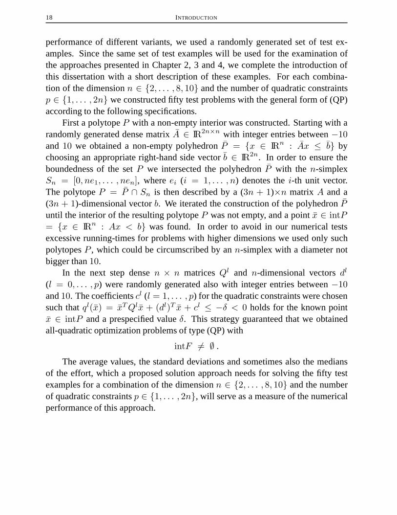
performance of different variants, we used a randomly generated set of test ex-amples. Since the same set of test examples will be used for the examination ofthe approaches presented in Chapter 2, 3 and 4, we complete the introduction ofthis dissertation with a short description of these examples. For each combina-tion of the dimensionn ∈ {2, . . . , 8, 10} and the number of quadratic constraintsp ∈ {1, . . . , 2n} we constructed fifty test problems with the general form of (QP)according to the following specifications.
First a polytopeP with a non-empty interior was constructed. Starting with arandomly generated dense matrixA ∈ IR2n×n with integer entries between−10and 10 we obtained a non-empty polyhedronP = {x ∈ IRn : Ax ≤ b} bychoosing an appropriate right-hand side vectorb ∈ IR2n. In order to ensure theboundedness of the setP we intersected the polyhedronP with the n-simplexSn = [0, ne1, . . . , nen], whereei (i = 1, . . . , n) denotes thei-th unit vector.The polytopeP = P ∩ Sn is then described by a (3n + 1)×n matrix A and a(3n + 1)-dimensional vectorb. We iterated the construction of the polyhedronPuntil the interior of the resulting polytopeP was not empty, and a pointx ∈ intP= {x ∈ IRn : Ax < b} was found. In order to avoid in our numerical testsexcessive running-times for problems with higher dimensions we used only suchpolytopesP , which could be circumscribed by ann-simplex with a diameter notbigger than10.
In the next step densen × n matricesQl and n-dimensional vectorsdl
(l = 0, . . . , p) were randomly generated also with integer entries between−10and10. The coefficientscl (l = 1, . . . , p) for the quadratic constraints were chosensuch thatql(x) = xTQlx + (dl)T x + cl ≤ −δ < 0 holds for the known pointx ∈ intP and a prespecified valueδ. This strategy guaranteed that we obtainedall-quadratic optimization problems of type (QP) with
intF 6= ∅ .
The average values, the standard deviations and sometimes also the mediansof the effort, which a proposed solution approach needs for solving the fifty testexamples for a combination of the dimensionn ∈ {2, . . . , 8, 10} and the numberof quadratic constraintsp ∈ {1, . . . , 2n}, will serve as a measure of the numericalperformance of this approach.

CHAPTER 2
Convergent Outer Approximation Algorithms forSolving Unary Problems
The first solution method for the all-quadratic Problem (QP), which we propose indetail in the present dissertation, is an indirect one. Instead of solving (QP) directlywe determine an optimal solution of a certain so-called unary problem, which isequivalent to (QP). Equivalence between (QP) and this unary problem holds in thesense that each solution of the unary problem yields a unique solution of the (QP)and vice versa.
This chapter deals with solution methods for general unary problems. Theseapproaches are derived from an outer approximation scheme introduced by Ra-mana [RAM 93]. Since the convergence of his approach cannot be guaranteed, itis the purpose of this chapter to develop solution methods which overcome thistheoretical deficiency.
2.1. Introduction
In order to introduce the class of unary problems we first have to clarify theconcept of unary matrices.
DEFINITION 2.1.1. A real symmetric matrixU ∈ IRn×n is called aunarymatrix, if and only if there exists a vectorv ∈ IRn with
U = vvT .
Denote by
Sn := { S ∈ IRn×n : S symmetric}the space of real symmetricn× n matrices and by
Un := { U ∈ Sn : U unary}19

20 CONVERGENT OUTER APPROXIMATION ALGORITHMS FORSOLVING UNARY PROBLEMS
the subset ofSn consisting of all unary matrices. Moreover, letU i ∈ Sn(i = 0, . . . , d) be given and letU : IRd → Sn be an affine matrix mapping de-fined by
U(z) = U0 +d∑i=1
ziUi , (2.1.1)
A unary problem is then defined as follows.
DEFINITION 2.1.2. Given U i ∈ Sn (i = 0, . . . , d) and h ∈ IRd,A = (a1, . . . , am)T ∈ IRm×d, b ∈ IRm, the optimization problem
min hT z
Az ≤ b
U(z) ∈ Un , z ∈ IRd(UP)
is called aunary problem.
REMARK 2.1.1. It is obvious (see Lemma 2.3.1) that the setUn of unary ma-trices consists of all positive semidefinite matricesU ∈ Sn with the additionalproperty
rank(U) = 1 .
Therefore, Problem (UP) can also be formulated as a semidefinite program withan additional rank constraint (for related discussion, see again [SHO87, RAM 93,PRW95, VB96, FK97] and Subsection 1.3.2).
As we will see in Section 2.2 it is possible to transform an all-quadratic prob-lem of type (QP) to an equivalent unary problem where the polyhedron
P := {z ∈ IRd : Az ≤ b}is bounded, i.e.,P is a polytope. Even though we discuss in this chapter solutionmethods for general problems of type (UP), our interest in Problem (UP) is onlymotivated by such problems which are equivalent transformations of all-quadraticproblems. Regarding the intention of this dissertation it is thus not a restriction toassume thatP is always bounded, as we have done in the sequel.
The equivalence between (QP) and a special problem of type (UP) is one ofthe interesting observations proposed without proof in the dissertation of Ramana

2.1. INTRODUCTION 21
[RAM 93, Chapter 7], which was our main motivation for considering unary prob-lems. In Section 2.2 a detailed proof of this equivalence is given. A second ob-servation suggested in Ramana’s research study is based on eigenvalue inequalitiesdue to Weyl: given an optimal vertex solutionz of the LP-relaxationminz∈P hT zof (UP) satisfyingU(z) /∈ Un, and given the eigenvalues ofU(z), a linear con-straint `(z) ≤ 0 can be constructed satisfying(z) > 0 and, for all z ∈ IRd
with U(z) ∈ Un, `(z) ≤ 0. Therefore, by adding successively such valid cuts`(z) ≤ 0 to LP-relaxations of (UP), one obtains an outer approximation (or cut-ting plane) algorithmic approach for solving (UP). Several variants of this cuttingplane approach together with some preliminary numerical results, which are reallypromising, are proposed in [RAM 93]. In Section 2.3 we compile some prelimi-naries underlying the basic ideas of this outer approximation approach and presentRamana’s algorithm.
A serious deficiency of this algorithmic approach, however, consists in the factthat cuts can possibly become very shallow. Therefore, the convergence of thesequence of optimal solutions of the outer approximations to an optimal solutionof (UP) cannot be guaranteed. A similar deficiency was observed in other cuttingplane methods for certain global optimization problems (see, e.g., [HT96B, Chap-ter 6]). By proposing alternative outer approximation algorithms for solving (UP),which are convergent in the sense that each accumulation point of the sequence ofoptimal solutions of the outer approximations is an optimal solution of (UP), weovercome the above deficiency.
As we will see in Section 2.4, it suffices in Problem (UP) with (2.1.1) to con-sider matricesU i ∈ Sn (i ∈ {1, . . . , d}), which form an orthonormal system withrespect to the inner product• : Sn × Sn → IR :
B • C = tr(BTC) =n∑
i,j=1
bijcij , (2.1.2)
whereB = (bij)1≤i,j≤n andC = (cij)1≤i,j≤n, andtr(A) =∑n
i=1 aii denotesthetraceof a matrixA ∈ IRn×n. Using this observation we derive in Section 2.4 avalid quadratic cut. This is a reverse convex constraint. For each optimal solutionz of an LP-relaxation of (UP) satisfyingU(z) /∈ Un, it cuts a sufficiently large ball(with respect to the Euclidean norm) centered atz out of the feasible region of thisLP-relaxation of (UP) without eliminating a feasible point of (UP), i.e., withoutaffecting the unarity.

22 CONVERGENT OUTER APPROXIMATION ALGORITHMS FORSOLVING UNARY PROBLEMS
If this cut is used directly in an outer approximation scheme, the convergenceof such a method can be guaranteed. Unfortunately, the direct use of this cut wouldlead to relaxations of (UP), which are as hard to solve as (UP) itself. If a suffi-ciently large polytope inscribed in the Euclidean norm ball is known, then we cancut this polytope out of the feasible region instead of the balls. Though the result-ing subproblems are still hard to solve, using the fact that a polytope is describedby a finite number of linear constraints, we obtain a convergent and practicable al-gorithm by building up this polytope by successive cutting planes. The basic ideaof this approach is presented in Section 2.5. The proposed algorithm is not a pureouter approximation scheme. It is a combination of an outer approximation and asuccessive subdivision of the feasible region of (UP).
In Section 2.6 we propose three possible ways to construct polytopes contain-ing a sufficiently large part of the intersection of the feasible region of an arbitraryLP-relaxation of (UP) and the relevant Euclidean norm ball. Each one of thesetypes of polytopes can then be used in order to obtain an implementable solutionscheme for (UP). In each iteration of these new algorithms we have to split a givenpolytope into a fixed number of subsets, and then we have to examine each of thesesubsets – as it is the case in branch-and-boundmethods (see, e.g., [HT96B, Chapter4]). From a numerical point of view this can lead to excessive storage requirements.In order to reduce the number of necessary splits and, thus, in order to reduce thenumber of generated polytopes, we develop in Section 2.7 a convergent algorithmwhich does not subdivide each considered polytope. The resulting method com-bines the cuts introduced by Ramana, a new cut introduced in Section 2.6 and thesubdivision strategy developed in Section 2.5. Most of the theoretical results ofSection 2.2 up to Section 2.6 were published in [HR98].
In the final Section 2.8 we discuss the numerical performance of the proposednew approaches. Since we are interested in solution methods for all-quadratic prob-lems we tried to solve the unary problems resulting from the equivalent transfor-mation of the problems belonging to our test set (see Section 1.5). Even thougha slight modification of the algorithms leads to a significant improvement of theirnumerical performance, our numerical results in Section 2.8 show that the practicalapplication of the unary problem approach to all-quadratic problems of type (QP)is limited to very small sizes.
2.2. UNARY PROBLEMS AND ALL-QUADRATIC OPTIMIZATION PROBLEMS 23
2.2. Unary Problems and All-Quadratic Optimization Problems
In this section it is shown that an arbitrary all-quadratic problem of type (QP) inn variables is equivalent to a unary problem ind =
(n+1
2
)+n variables. By reasons
which will become evident in Section 2.4, we choose a transformation which yieldsa unary problem, where the matricesU i (i = 1, . . . , d) form an orthonormal systemwith respect to the inner matrix product (2.1.2).
As usual we have used in the formulation of (QP) as well as in the formulationof (UP) the lettersA andb, respectivelyP for describing the linear constraints. Inorder to avoid ambiguities we add the superscriptQ, if a letter is related to Problem(QP), and the superscriptU otherwise.
Consider an arbitrary all-quadratic problem of type (QP), i.e., consider theproblem
min xTQ0x+ (d0)Tx
xTQlx+ (dl)Tx+ cl ≤ 0 l = 1, . . . , p
AQx ≤ bQ , x ∈ IRn ,
(QP)
whereQl = (qlij)1≤i,j≤n ∈ Sn, dl ∈ IRn (l = 0, . . . , p), cl ∈ IR (l = 1, . . . , p),AQ = (aQ1 , . . . , a
Qm)T ∈ IRm×n and bQ ∈ IRm. Since we assumed that
PQ = {x ∈ IRn : AQx ≤ bQ} is a polytope we know that there exists a hyper-rectangleRQ = {x ∈ IRn : lQ ≤ x ≤ LQ} with lQ, LQ ∈ IRn satisfying
PQ ⊂ RQ .
Let ei ∈ IRn+1 denote thei-th unit vector (i = 1, . . . , n + 1), and letEij ∈ IR(n+1)×(n+1) be the elementary matrix with entry1 at position(i, j) and0at any other position. The equivalent transformation of Problem (QP) leads to thefollowing unary problem
min hT z
AUz ≤ bU
lU ≤ z ≤ LU
U(z) ∈ Un+1 , z ∈ IR(
n+12
)+n
(UP)
in the variablez = (z11, . . . , z1n, z1,n+1, z22, . . . , z2,n+1, . . . , znn, zn,n+1)T ,
where, fori = 1, . . . , n,

24 CONVERGENT OUTER APPROXIMATION ALGORITHMS FORSOLVING UNARY PROBLEMS
hi,n+1 = 1√2d0i , a
Ul,(i,n+1) = 1√
2dli (l = 1, . . . , p),
aUp+l,(i,n+1) = 1√2aQli (l = 1, . . . ,m),
lUi,n+1 =√
2lQi , LUi,n+1 =√
2LQi ,
hii = q0ii , aUl,ii = qlii (l = 1, . . . , p) ,
aUp+l,ii = 0 (l = 1, . . . ,m),
lUii = max{(min{LQi , 0})2 , (max{lQi , 0})2} , LUii = max{lQi lQi , LQi LQi },and, for1 ≤ i < j ≤ n,hij =
√2q0ij , a
Ul,ij =
√2qlij (l = 1, . . . , p) , aUp+l,ij = 0 (l = 1, . . . ,m),
lUij =√
2 min{lQi lQj , lQi LQj , LQi lQj , LQi LQj },LUij =
√2max{lQi lQj , lQi LQj , LQi lQj , LQi LQj }.
The right-hand sidebU of the linear constraints is given by
bUl = −cl (l = 1, . . . , p) , bUp+l = bQl (l = 1, . . . ,m) ,
and the affine matrix mapping in (UP) is defined as follows
U : IR(
n+12
)+n → Sn :⇔
U(z) = U0 +n∑i=1
ziiUii +
∑1≤i<j≤n+1
zijUij
(2.2.1)
with U0 = En+1,n+1, U ii = Eii (i = 1, . . . , n) andU ij = 1√2(Eij + Eji)
(1 ≤ i < j ≤ n+ 1).A quadratic function consists of three different terms of variables. There are
linear terms (xi, i = 1, . . . , n), pure quadratic terms (x2i , i = 1, . . . , n) and bilinear
terms (xixj , 1 ≤ i < j ≤ n). In the formulation of (UP) each of these terms isreplaced by a new variable such that all functions involved in the formulation of(QP) can be transformed to linear functions. The additional unarity condition in(UP) guarantees that each feasible point of (UP) coincides with a feasible point of(QP). For that reason the postulated equivalence between the all-quadratic problem(QP) and the unary problem (UP) holds in the sense of the following theorem.

2.2. UNARY PROBLEMS AND ALL-QUADRATIC OPTIMIZATION PROBLEMS 25
THEOREM 2.2.1. Let x? be an optimal solution of Problem (QP) and letz?
be an optimal solution of Problem (UP). If we set
zi,n+1 =√
2x?i , zii = (x?i )2 (i = 1, . . . , n) , zij =
√2x?i x
?j (1 ≤ i < j ≤ n) ,
and
xi =1√2z?i,n+1 (i = 1, . . . , n) ,
thenz is a feasible solution of Problem (UP), x is a feasible solution of Problem(QP) and
(x)TQ0x+ (d0)T x = (x?)TQ0x? + (d0)Tx? = hT z = hT z? . (2.2.2)
PROOF: Straightforward calculation shows that
U(z) =(x?
1
)((x?)T , 1) ,
and henceU(z) ∈ Un+1. By the definition oflU andLU and the fact thatx? iscontained inRQ it follows immediately
lU ≤ z ≤ LU .
For thel-th rowaUl of the matrixAU we obtain, forl = 1, . . . , p,
aUl z =n∑i=1
aUl,(i,n+1)zi,n+1 +∑
1≤i≤j≤naUl,ij zij =
n∑i=1
dlix?i +
n∑i,j=1
qlijx?i x?j
= (x?)TQlx? + (dl)Tx? ≤ −cl = bUl ,
and, forl = 1, . . . ,m,
aUp+lz =n∑i=1
aUp+l,(i,n+1)zi,n+1 +∑
1≤i≤j≤naUp+l,ij zij︸ ︷︷ ︸
=0
= (aQl )Tx? ≤ bQl = bUp+l ,
i.e., z is a feasible solution of Problem (UP). Similar direct calculations show that
hT z = (x?)TQ0x? + (d0)Tx? ,
and hence, sincez satisfies the constraints of (UP) andz? is an optimal solution of(UP), we obtain
hT z? ≤ (x?)TQ0x? + (d0)Tx? .

26 CONVERGENT OUTER APPROXIMATION ALGORITHMS FORSOLVING UNARY PROBLEMS
Analogously one easily obtains thatx is feasible for (QP) and hT z? =(x)TQ0x+ (d0)T x, which implies that
hT z? ≥ (x?)TQ0x? + (d0)Tx? .�
REMARK 2.2.1. As mentioned in Remark 2.1.1, Problem (UP) can also beinterpreted as a special semidefinite program. Using the semidefinite programmingnotations a short formulation of the previous theorem is available along the linesgiven, e.g., in [RAM 93, PRW95, VB96, FK97]. In order to avoid the introductionof these semidefinite programming notations we decided to use the presented moretechnical version of the equivalence result.
Example. We conclude this section with a simple example. Consider theone-dimensional all-quadratic problem
min x2 + x
−x2 + 1 ≤ 0
x ∈ [−2, 2] .
(QPE)
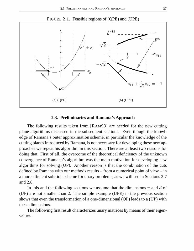
The feasible regionFQ of (QPE) is given by the two disjoint intervals[−2,−1]and[1, 2], and the optimal solutionx? is−1 (see Figure 2.1(a)) with optimal value0. Using the described transformation we obtain the following unary problem
min z11 + 1√2z12
−z11 ≤ − 1
0 ≤ z11 ≤ 4
−2√
2 ≤ z12 ≤ 2√
2(0 00 1
)+ z11
(1 00 0
)+ z12
(0 1√
21√2
0
)∈ U2 .
(UPE)
The optimal value of (UPE) is also0 and is attained at the unique solution pointz? = (1,−√2)T belonging to the feasible regionFU of (UPE) given by
FU = {z ∈ IR2 : 1 ≤ z11 ≤ 4 , −2√
2 ≤ z12 ≤ 2√
2 , z212 = 2z11}
(see the two disjoint arcs in Figure 2.1(b)). We will use Problem (UPE) throughoutthis chapter in order to illustrate the proposed solution methods.
Note that in the following sections we consider only unary problems. There-fore, the superscriptU is not necessary any more.
2.3. PRELIMINARIES AND RAMANA’ S APPROACH 27
FIGURE 2.1. Feasible regions of (QPE) and (UPE)
x−1 1x?
1
FQ
x2 + x
(a) (QPE)
z12
√2
FU
2 z11
−√2z?
z11 + 1√2z12 = −1
(b) (UPE)
2.3. Preliminaries and Ramana’s Approach
The following results taken from [RAM 93] are needed for the new cuttingplane algorithms discussed in the subsequent sections. Even though the knowl-edge of Ramana’s outer approximation scheme, in particular the knowledge of thecutting planes introduced by Ramana, is not necessary for developing these new ap-proaches we repeat his algorithm in this section. There are at least two reasons fordoing that. First of all, the overcome of the theoretical deficiency of the unknownconvergence of Ramana’s algorithm was the main motivation for developing newalgorithms for solving (UP). Another reason is that the combination of the cutsdefined by Ramana with our methods results – from a numerical point of view – ina more efficient solution scheme for unary problems, as we will see in Sections 2.7and 2.8.
In this and the following sections we assume that the dimensionsn andd of(UP) are not smaller than2. The simple example (UPE) in the previous sectionshows that even the transformation of a one-dimensional (QP) leads to a (UP) withthese dimensions.
The following first result characterizes unary matrices by means of their eigen-values.

28 CONVERGENT OUTER APPROXIMATION ALGORITHMS FORSOLVING UNARY PROBLEMS
LEMMA 2.3.1. LetU ∈ Sn, and letλi(U) (i = 1, . . . , n) be the eigenvaluesofU indexed in increasing order. Then the following assertions are equivalent:
(i) U ∈ Un;(ii) λi(U) = 0, i = 1, . . . , n− 1;(iii) λ1(U) ≥ 0 and λn−1(U) ≤ 0;(iv) λ1(U) ≥ 0 and tr(U) ≤ λn(U).
PROOF: The above equivalences follow readily from the well–known factsthat a matrixU ∈ IRn×n is unary if and only if it is positive semidefinite andrank(U) = 1, and that, for each realn × n matrix A, there holdstr(A) =∑n
i=1 λi(A) (see, e.g., [ZUR64, §13]). �
The second lemma describes now a relation between the eigenvalues of thesum of symmetric matrices and the sum of the eigenvalues of these matrices.
LEMMA 2.3.2. LetE,F ∈ Sn with eigenvaluesλi(E), λi(F ) (i = 1, . . . , n)be indexed in the same order as above. Then, for eachk ∈ {1, . . . , n}, there holds
λ1(E) + λk(F ) ≤ λk(E + F ) ≤ λk(E) + λn(F ) . (2.3.1)
PROOF: See, e.g., [HJ85]. �
This result is due to Hermann Weyl. Therefore, we will denote the inequal-ities (2.3.1) asWeyl’s inequalities. Using the result of the last lemma a relationbetween the eigenvalues of the affine matrix mappingU(·) and the eigenvalues ofthe matricesU i (i = 0, . . . , n) formingU(·) was derived in [RAM 93].
COROLLARY 2.3.3. LetU : IRd → Sn be an affine matrix mapping definedas in (2.1.1). Then, for every nonnegativey ∈ IRd+ andk ∈ {1, . . . , n}, there holds
λk(U(y)) ≤ λk(U0) +d∑i=1
yiλn(U i)
and
λk(U(y)) ≥ λk(U0) +d∑i=1
yiλ1(U i) ,
where all eigenvaluesλi(·) (i = 1, . . . , n) are indexed in ascending order.
2.3. PRELIMINARIES AND RAMANA’ S APPROACH 29
PROOF: The results follow by successive application of Weyl’s inequalities(Lemma 2.3.2) and the fact that, for eachU ∈ Sn, µ ≥ 0 andi ∈ {1, . . . , n}, thereholdsλi(µU) = µλi(U). �
Consider now the LP-relaxation
min hT z
Az ≤ b(UPL)
of (UP), which arises from (UP) by omitting the unary conditionU(z) ∈ Un. Givena vertex optimal solutionz of (UPL) and the affine matrix mappingU defined in(2.1.1),λ1(U(z)) = 0 andλn−1(U(z)) = 0 implies thatz is an optimal solutionof (UP) because of Lemma 2.3.1. Otherwise, one must haveλ1(U(z)) < 0 orλn−1(U(z)) > 0 (or both). In this case, however, Corollary 2.3.3 allows oneto construct an additional linear constraint`(z) ≤ 0 which, when added to theconstraints of (UPL), is violated byz but satisfied by all feasible solutions of (UP).
Since z is a vertex solution of a linear program it is known thatz is theunique solution of a nonsingulard × d system of linear equations binding atz,which – following the standard terminology in simplex algorithms – will be calleda nonsingular basic system corresponding toz. Simplex-type algorithms pro-vide such a system automatically. In order to derive the linear cuts introduced in[RAM 93] letBz ≤ r be the corresponding nonsingular basic system forz satis-fying Bz = r. By the definition of the corresponding nonsingular basic systemwe know that each pointz ∈ P = {z ∈ IRd : Az ≤ b} is contained in the coneC := {z ∈ IRd : Bz ≤ r} (C is the smallest of such cones containingP anduniquely determined whenz is a non-degenerate vertex ofP ). Choose an arbitrarypointz ∈ P and set
y := r −Bz .
The pointy is a nonnegative element ofIRd, and for the affine matrix mappingU(·)at the pointz we obtain
U(z) = U(B−1r︸ ︷︷ ︸=z
−B−1y) = U(z) +d∑i=1
yi(U0 − U(B−1ei)
), (2.3.2)
whereei ∈ IRd denotes again thei-th unit vector (i = 1, . . . , d). The right-handside of (2.3.2) is an affine matrix mapping with the form given in (2.1.1). Therefore,

30 CONVERGENT OUTER APPROXIMATION ALGORITHMS FORSOLVING UNARY PROBLEMS
Corollary 2.3.3 is applicable, and we obtain
λn−1(U(z)) ≥ λn−1(U(z)) +d∑i=1
yi λ1
(U0 − U(B−1ei)
)and
λ1(U(z)) ≤ λ1(U(z)) +d∑i=1
yi︸︷︷︸=(r−Bz)i
λn(U0 − U(B−1ei)
).
It follows that, for each pointz ∈ P with U(z) ∈ Un, the cut
d∑i=1
(r −Bz)i λ1
(U0 − U(B−1ei)
)+ λn−1(U(z)) ≤ 0 (2.3.3)
is valid. However, for the pointz with λn−1(U(z)) > 0, (2.3.3) is violated.An analogous result is true for the linear constraint
d∑i=1
(Bz − r)i λn(U0 − U(B−1ei)
)− λ1(U(z)) ≤ 0 . (2.3.4)
Adding these cuts to the linear constraints describingP we obtain a better outerapproximation of the feasible region of (UP) and we can calculate a new, maybebetter, vertex solution of this new LP-relaxation of (UP). Continuing in this way,a polyhedral outer approximation (or cutting plane) approach is obtained which,in each iteration, requires only solving linear programs and eigenvalue calcula-tions. Based on the above arguments, Ramana [RAM 93] proposed the followingapproach.
ALGORITHM 2.1 (Ramana’s Algorithm for Solving (UP) ).
InitializationP 0 ← {z ∈ IRd : Az ≤ b}, STOP← False, k ← 0
While STOP =False DoIf P k = ∅ Then
STOP← True (P ∩ {z ∈ IRd : U(z) ∈ Un} = ∅)Else
Solve the linear optimization problemminz∈Pk hT z to obtain a vertex
solutionzk and a corresponding nonsingular basic systemBkz ≤ rksatisfyingBkzk = rk.

2.3. PRELIMINARIES AND RAMANA’ S APPROACH 31
Compute the eigenvalues ofU(zk) indexed in increasing order.
If λ1(U(zk)) ≥ 0 AND λn−1(U(zk)) ≤ 0 ThenSTOP← True (zk is an optimal solution of (UP))
ElseIf λn−1(U(zk)) > 0 Then
(a1)ki ← −λ1
(U0 − U((Bk)−1ei)
), i = 1, . . . , d
(β1)k ← −λn−1(U(zk))P k ← P k ∩ {z ∈ IRd : ((a1)k)TBkz ≤ ((a1)k)TBkzk + (β1)k}
EndIfIf λ1(U(zk)) < 0 Then
(a2)ki ← λn(U0 − U((Bk)−1ei)
), i = 1, . . . , d
(β2)k ← λ1(U(zk))P k ← P k ∩ {z ∈ IRd : ((a2)k)TBkz ≤ ((a2)k)TBkzk + (β2)k}
EndIfP k+1 ← P k, k ← k + 1
EndIfEndIf
EndWhile
Example. Consider again Problem (UPE). The first vertex solutionz0 is ob-viously given by(1,−2
√2)T (see Figure 2.1(b)). The corresponding nonsingular
basic system is ( −1 00 −1
)(z11z12
)≤( −1
2√
2
).
For the eigenvalues ofU(·) at z0 we obtain
λ1(U(z0)) = λn−1(U(z0)) = −1 .
The linear cut (2.3.4) is hence defined by
−z11 − 1√2z12 ≤ 0 ,
and for the new outer approximationP 1 of the feasible region of (UPE) it followsP 1 = {z ∈ IR2 : 1 ≤ z11 ≤ 4 , −2
√2 ≤ z12 ≤ 2
√2 , −z11 − 1√
2z12 ≤ 0} (see
Figure 2.2).

32 CONVERGENT OUTER APPROXIMATION ALGORITHMS FORSOLVING UNARY PROBLEMS
FIGURE 2.2. Ramana’s cut for (UPE)
������������������������������������������������������������������������������������������������
������������������������������������������������������������������������������������������������
z12
√2
2z11
−√2
z0
P 1
z1
If Algorithm 2.1 stops after a finite number of iterations with a pointzk, re-spectively by detecting the emptiness ofP k, then it is obvious in view of the pre-vious considerations thatzk is an optimal solution of (UP), respectively that thefeasible region of (UP) is empty. Up to now it is an open question, whether Algo-rithm 2.1 is convergent in the sense that each accumulation pointz? of the sequence{zk}k∈IN satisfiesz? ∈ {z ∈ IRd : Az ≤ b, U(z) ∈ Un}. Since the sequences{((aj)k)TBk}k∈IN (j = 1, 2) might fail to be bounded, it does not seem that theconvergence of Algorithm 2.1 can be guaranteed. For a related convergence theoryof cutting plane algorithms in global optimization we refer to [HT96B].
REMARK 2.3.1. By applying another cutting plane for the case that the small-est eigenvalue ofU(zk) is smaller than0, Ramana was able to derive at least apartial convergence result. Letwk be a normalized eigenvector ofU(zk) corre-sponding to the smallest eigenvalue of this matrix. The linear cut
(wk)TU(z)wk =d∑i=1
((wk)TU iwk
)zi + (wk)TU0wk ≥ 0 (2.3.5)
is applicable, since there holds(wk)TU(zk)wk = λ1(U(zk)) < 0, and, for eachz ∈ IRd with U(z) ∈ Un, it follows (wk)TU(z)wk ≥ 0. Note that each matrixU ∈ Un must be positive semidefinite. If in Algorithm 2.1 the cut (2.3.5) is usedinstead of (2.3.4) and if the caseλn−1(U(zk)) > 0 occurs only a finite number of

2.4. VALID CUTS FORCONVERGENT OUTER APPROXIMATION ALGORITHMS 33
times, then it is provable (see [RAM 93, pages 93f]) that this algorithm is convergentin the required sense.
It is the aim of the subsequent sections to overcome the above theoretical defi-ciency of Algorithm 2.1 by developing other in each case convergent outer approx-imation approaches for solving (UP).
2.4. Valid Cuts for Convergent Outer Approximation Algorithms
A first step towards convergent outer approximation algorithms for solving(UP) consists in requiring that in the affine matrix mapping (2.1.1)
U : IRd → Sn :⇔ U(z) = U0 +d∑i=1
ziUi ,
the matricesU i (i = 1, . . . , d) form an orthonormal system (ONS) with respectto the inner product (2.1.2). This is not a real restriction for the generality of theconsidered problems of type (UP). Each unary problem of this type is equivalentto another unary problem which fulfills this additional condition. This is the resultof the following lemma.
LEMMA 2.4.1. Let an arbitrary unary problem
min hT z
Az ≤ b
U(z) ∈ Un , z ∈ IRd(UP1)
with h ∈ IRd, A ∈ IRm×d and U : IRd → Sn, U(z) = U0 +∑d
i=1 ziUi be
given. Then there exist a dimensiond ≤ d, vectorsh1 ∈ IRd, h2 ∈ IRd−d, matricesA1 ∈ IRm×d,A2 ∈ IRm×(d−d) and an ONS{U i, i = 1, . . . , d} with respect to theinner product• defined in (2.1.2) such that the optimization problem
min hT1 x+ hT2 y
A1x+A2y ≤ b
U(x) = U0 +d∑i=1
xiUi ∈ Un
x ∈ IRd , y ∈ IRd−d
(UP2)
is equivalent to (UP1).

34 CONVERGENT OUTER APPROXIMATION ALGORITHMS FORSOLVING UNARY PROBLEMS
PROOF: Determine a maximal linearly independent subset
{U ij , j = 1, . . . , d} ⊂ {U i, i = 1, . . . , d}(so that the two linear spaces generated by theU ij respectively theU i have equaldimension). Assume, for ease, that there holds{i1, . . . , id} = {1, . . . , d}. ThematricesU j (j ∈ {d + 1, . . . , d}) are contained in the linear space generated bythe matricesU i (i = 1, . . . , d). Therefore, there exists, for eachj ∈ {1, . . . , d−d},a vectorλj ∈ IRd with
Ud+j =d∑i=1
λji Ui .
SetL = (λ1, . . . , λd−d) ∈ IRd×(d−d). Use now the Gram-Schmidt procedure(see, e.g., [GVL89, Chapter 5]) in order to generate from{U i, i = 1, . . . , d} acorresponding ONS{U i, i = 1, . . . , d}. Let, for i ∈ {1, . . . , d}, µi ∈ IRd be theunique vector satisfying
U i =d∑j=1
µijUj .
Since the function which maps theU i onto theU j (j = 1, . . . , d) is a homeo-morphism we know that the matrixM = (µ1, . . . , µd) ∈ IRd×d is regular. Letz = (z, z)T with z ∈ IRd and z ∈ IRd−d be an arbitrary element ofIRd. Let,furthermore, the matrixA ∈ IRm×d be given byA = (A, A) with A ∈ IRm×d andA ∈ IRm×(d−d), and the vectorh ∈ IRd be given byh = (h, h)T ∈ IRd+(d−d). Set
x = M(z + Lz) , y = z ,
A1 = AM−1 , A2 = A− ALand
h1 = (M−1)T h , h2 = h− LT h .
Then it follows
hT z = hT z + hT z = hT (M−1x− Lz) + hT z = hT1 x+ hT2 y ,
Az = Az + Az = A(M−1x− Lz) + Az = A1x+A2y ,

2.4. VALID CUTS FORCONVERGENT OUTER APPROXIMATION ALGORITHMS 35
and
U(z) = U0 +d∑i=1
ziUi +
d∑i=d+1
ziUi = U0 +
d∑i=1
zi +
d∑j=d+1
zjλji
U i
= U0 +d∑l=1
d∑i=1
µil(zi +d∑
j=d+1
zjλji )
︸ ︷︷ ︸=(M(z+Lz))l =xl
U l = U(x) .
Since the matrixM is regular the previous calculations demonstrate a one-to-onerelation between the feasible points of (UP1) and (UP2). This shows the equiva-lence of both problems. �
Even though Problem (UP2) has a more general form than Problem (UP) wewill develop the following theory and solution methods only for unary problems oftype (UP). This is motivated on the one hand by the fact that the transformationpresented in Section 2.2, which links the all-quadratic problems of type (QP) toequivalent problems of type (UP), yields an ONS{U ij , 1 ≤ i ≤ j < n + 1} in(2.2.1). Since it is the purpose of this research study to develop solution methods for(QP) it is, therefore, sufficient to consider the more restricted form (UP) of unaryproblems instead of (UP2). On the other hand, the following theory and solutionmethods can be extended by slight changes to problems of type (UP2). However,this leads to increasing technical effort, what we would like to avoid.
The following lemma shows the postulated fact that the matricesU ij
(1 ≤ i ≤ j < n + 1) defined in (2.2.1) form an ONS with respect to the innerproduct given by (2.1.2).
LEMMA 2.4.2. Let Eij = eieTj ∈ IR(n+1)×(n+1) (i, j = 1, . . . , n + 1) be
given as in Section 2.2. Then the matrices
U ii = Eii , i = 1, . . . , n
U ij = 1√2(Eij + Eji) , 1 ≤ i < j ≤ n+ 1
form an ONS with respect to the inner product• defined in (2.1.2).
PROOF: This result can be verified by straightforward calculations. �

36 CONVERGENT OUTER APPROXIMATION ALGORITHMS FORSOLVING UNARY PROBLEMS
With the orthonormal property of the set{U i, i = 1, . . . , d} we are now ableto derive a relation between the Euclidean distance of two pointsz, z ∈ IRd andthedistancebetween the two corresponding matricesU(z) andU(z). In order tomeasure thedistancebetween two matrices we use a suitable matrix norm. Let‖A‖F =
√A •A (A ∈ Sn) denote the norm induced by the inner product (2.1.2)
– the so-calledFrobenius-norm.
LEMMA 2.4.3. Let{U i, i = 1, . . . , d} ⊂ Sn form an ONS with respect to theinner product• defined in (2.1.2). Then, for eachz, z ∈ IRd, there holds
‖d∑i=1
(z − z)iU i‖F = ‖z − z‖2 . (2.4.1)
PROOF: By the orthonormality of{U i, i = 1, . . . , d} we know that, for eachi, j ∈ {1, . . . , d}, there holds
tr((U i)TU j
)= U i • U j =
{1 , if i = j
0 , otherwise.
Thus, for eachz, z ∈ IRd, it follows
‖d∑i=1
(z − z)iU i‖2F = tr
((d∑i=1
(z − z)iU i)T (d∑i=1
(z − z)iU i))
=d∑
i,j=1
(z − z)i(z − z)j tr((U i)TU j
)
=d∑i=1
(z − z)2i = ‖z − z‖22 .
�
The combination of (2.4.1) with Weyl’s inequalities (2.3.1) allows us to provethat for arbitrary pointsz, z ∈ IRd the distance between the eigenvalues ofU(z)andU(z) is at least as big as the Euclidean distance between these points. With thisresult of the following theorem we will develop a valid cut for a convergent outerapproximation algorithm.
THEOREM 2.4.4. Let {U i, i = 1, . . . , d} ⊂ Sn form an ONS with respect tothe inner product• defined in (2.1.2), and letU : IRd → Sn be an affine matrix

2.4. VALID CUTS FORCONVERGENT OUTER APPROXIMATION ALGORITHMS 37
mapping of the form
z → U(z) = U0 +d∑i=1
ziUi
withU0 ∈ Sn. Assume that the eigenvalues of the matrices involved are indexed inan increasing order. Then, for eachz, z ∈ IRd, there holds
λn−1 (U(z)) ≥ λn−1 (U(z))− ‖z − z‖2 (2.4.2)and
λ1 (U(z)) ≤ λ1 (U(z)) + ‖z − z‖2 . (2.4.3)
PROOF: Since the Frobenius norm is an upper bound for the spectral radiusρ(S) = max{|λ|, λ eigenvalue ofS} (S ∈ Sn) (see, e.g., [ZUR64]), one obtainsby means of Lemma 2.3.2
λn−1(U(z)) = λn−1(U(z − z) + U(z)− U0) = λn−1(d∑i=1
(z − z)iU i + U(z))
≥ λn−1(U(z)) + λ1(d∑i=1
(z − z)iU i)
≥ λn−1(U(z))− ‖d∑i=1
(z − z)iU i‖F = λn−1(U(z))− ‖z − z‖2 .
Similarly, inequality (2.4.3) follows from
λ1(U(z)) = λ1(U(z − z) + U(z)− U0) = λ1(d∑i=1
(z − z)iU i + U(z))
≤ λ1(U(z)) + λn(d∑i=1
(z − z)iU i)
≤ λ1(U(z)) + ‖d∑i=1
(z − z)iU i‖F = λ1(U(z)) + ‖z − z‖2 .
�
REMARK 2.4.1. The result of Theorem 2.4.4 can also be derived by a combi-nation of Lemma 2.4.3 and the Hoffman-Wielandt inequality given in [HW53].Indeed, letA,B ∈ Sn be two arbitrary matrices with eigenvaluesα1, . . . , αnandβ1, . . . , βn indexed in increasing order. The Hoffman-Wielandt inequality in[HW53] says that there is a permutationπ : {1, . . . , n} → {1, . . . , n} satisfying
n∑i=1
|αi − βπ(i)|2 ≤ ‖A−B‖2F . (2.4.4)

38 CONVERGENT OUTER APPROXIMATION ALGORITHMS FORSOLVING UNARY PROBLEMS
If we denote byΠ the set of all permutations of{1, . . . , n}, then (2.4.4) is equiva-lent to
minπ∈Π
n∑i=1
|αi − βπ(i)|2 ≤ ‖A−B‖2F .
Setα = (α1, . . . , αn)T andβ = (β1, . . . , βn)T . It can be proven by an inductionwith respect to the dimensionn that there holds
maxπ∈Π
n∑i=1
αiβπ(i) = αTβ .
Using this fact we obtain
minπ∈Π
n∑i=1
|αi − βπ(i)|2 = ‖α‖22 + ‖β‖22 − 2 maxπ∈Π
n∑i=1
αiβπ(i)
= ‖α− β‖22 ,
and in view of (2.4.4) it follows, for eachi ∈ {1, . . . , n},|αi − βi| ≤ ‖A−B‖F . (2.4.5)
If we apply this relation to the situation of Theorem 2.4.4, the use of Lemma 2.4.3yields the inequalities (2.4.2) and (2.4.3).
As in the description of Ramana’s cuts introduced in the previous section, letz ∈ IRd be an optimal solution of an LP-relaxation of (UP) satisfyingU(z) /∈ Un.In view of Lemma 2.3.1(iii) we know that
ε(z) := max {λn−1(U(z)),−λ1(U(z))}must be greater than0. From Theorem 2.4.4 it follows that each pointz ∈ IRd
contained in a ball (with respect to the Euclidean norm), which has a radius equalto ε(z) and is centered atz, cannot be feasible for (UP). Therefore, we see that
`z(z) := ε(z)− ‖z − z‖2 ≤ 0 (2.4.6)
is a valid cut, i.e., we knowz(z) > 0, and, for eachz ∈ IRd with U(z) ∈ Un,there holds z(z) ≤ 0.
Example. In the situation of Problem (UPE) we know thatz = (1,−2√
2)T
is an optimal solution of an LP-relaxation of this problem withε(z) = 1 (see page31). In view of the above arguments it follows that each point contained in the

2.4. VALID CUTS FORCONVERGENT OUTER APPROXIMATION ALGORITHMS 39
FIGURE 2.3. First quadratic cut for (UPE)
������������������������������������������������������������
������������������������������������������������������������
z11
z12
√2
2
zC
−√2
circleC centered atz with radius1 (see Figure 2.3) is not feasible for (UPE).
If we replace in Ramana’s Algorithm 2.1 the linear cuts used there by`zk(z) ≤ 0, then we obtain a convergent outer approximation algorithm for solving(UP), as the following theorem shows.
THEOREM 2.4.5. Let {zk}k∈IN be a sequence of points in the polytopeP = {z ∈ IRd : Az ≤ b} satisfying, for eachk, i ∈ IN with k < i,
`zk(zi) ≤ 0 . (2.4.7)
Then every accumulation pointz? of {zk}k∈IN satisfiesU(z?) ∈ Un.
PROOF: Let z? be an accumulation point of the sequence{zk}k∈IN and let{zkq}q∈IN be a subsequence converging toz?. From (2.4.7) it follows that, for eachq ∈ IN, we know that
`zkq (zkq+1) ≤ 0 .
Since‖zkq+1 − zkq‖2 → 0 (q →∞), this relation implies – in view of (2.4.6) andbecause ofmax{λn−1(U(zkq)),−λ1(U(zkq))} ≥ 0 (q ∈ IN) – that there holds
max {λn−1(U(zkq)),−λ1(U(zkq))} → 0 (q →∞) .
From this ensues
λ1(U(z?)) = λn−1(U(z?)) = 0
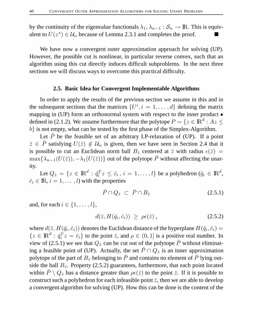
40 CONVERGENT OUTER APPROXIMATION ALGORITHMS FORSOLVING UNARY PROBLEMS
by the continuity of the eigenvalue functionalsλ1, λn−1 : Sn → IR. This is equiv-alent toU(z?) ∈ Un because of Lemma 2.3.1 and completes the proof. �
We have now a convergent outer approximation approach for solving (UP).However, the possible cut is nonlinear, in particular reverse convex, such that analgorithm using this cut directly induces difficult subproblems. In the next threesections we will discuss ways to overcome this practical difficulty.
2.5. Basic Idea for Convergent Implementable Algorithms
In order to apply the results of the previous section we assume in this and inthe subsequent sections that the matrices{U i, i = 1, . . . , d} defining the matrixmapping in (UP) form an orthonormal system with respect to the inner product•defined in (2.1.2). We assume furthermore that the polytopeP = {z ∈ IRd : Az ≤b} is not empty, what can be tested by the first phase of the Simplex-Algorithm.
Let P be the feasible set of an arbitrary LP-relaxation of (UP). If a pointz ∈ P satisfyingU(z) /∈ Un is given, then we have seen in Section 2.4 that itis possible to cut an Euclidean norm ballBz centered atz with radiusε(z) =max{λn−1(U(z)),−λ1(U(z))} out of the polytopeP without affecting the unar-ity.
Let Qz = {z ∈ IRd : qTi z ≤ ci , i = 1, . . . , l} be a polyhedron (qi ∈ IRd,ci ∈ IR, i = 1, . . . , l) with the properties
P ∩Qz ⊂ P ∩Bz (2.5.1)
and, for eachi ∈ {1, . . . , l},d(z, H(qi, ci)) ≥ ρε(z) , (2.5.2)
whered(z, H(qi, ci)) denotes the Euclidean distance of the hyperplaneH(qi, ci) ={z ∈ IRd : qTi z = ci} to the pointz, andρ ∈ (0, 1] is a positive real number. Inview of (2.5.1) we see thatQz can be cut out of the polytopeP without eliminat-ing a feasible point of (UP). Actually, the setP ∩ Qz is an inner approximationpolytope of the part ofBz belonging toP and contains no element ofP lying out-side the ballBz . Property (2.5.2) guarantees, furthermore, that each point locatedwithin P \ Qz has a distance greater thanρε(z) to the pointz. If it is possible toconstruct such a polyhedron for each infeasible pointz, then we are able to developa convergent algorithm for solving (UP). How this can be done is the content of the

2.5. BASIC IDEA FOR CONVERGENT IMPLEMENTABLE ALGORITHMS 41
present section. In the next section we will propose three different possibilities forconstructing appropriate polyhedra.
Assume now that for each pointz belonging to a polytopeP ⊂ P and satis-fying U(z) /∈ Un a polyhedronQz with Properties (2.5.1) and (2.5.2) is known.Of course we cannot cut the setQz out of P in one step. The closure ofP \ Qzis not necessarily a polytope and, thus, an algorithm doing this would induce diffi-cult subproblems, as it is the case by using the quadratic cut directly. However, incontrast to the Euclidean norm ballBz the polyhedronQz is described by a finitenumber of linear constraints. If we constructl new polytopesPi (i = 1, . . . , l) byadding one of the constraints describingQz to the constraints describingP , thenwe know that the union of thePi’s (i = 1, . . . , l) contains no point of the interiorof Qz, but all feasible elements ofP . Applying this strategy the algorithm is asfollows.
ALGORITHM 2.2 (Basic Convergent Algorithm for Solving (UP)).Initialization
Chooseρ ∈ (0, 1] andl ∈ IN, and setP 0 ← {z ∈ IRd : Az ≤ b}.Solve the linear optimization problem (LP)minz∈P 0 hT z, and letz0 be an
optimal solution with optimal valueµP 0 = hT z0.
µ0 ← µP 0 , P ← {P 0}, STOP← False, k ← 0
While STOP =False DoCompute the eigenvalues ofU(zk) indexed in increasing order.
If λ1(U(zk)) ≥ 0 AND λn−1(U(zk)) ≤ 0 Then (SC1)
STOP← True (zk is an optimal solution of (UP))
Elseε(zk)← max {λn−1(U(zk)),−λ1(U(zk))}Construct a polyhedronQk = {z ∈ IRd : (qki )
T z ≤ cki , i = 1, . . . , l}satisfying
P k ∩Qk ⊂ P k ∩ {z ∈ IRd : ‖z − zk‖2 ≤ ε(zk)} (PR1)
and, for eachi ∈ {1, . . . , l},d(zk, H(qki , c
ki )) = |(qk
i )T zk−cki |
‖qki‖2
≥ ρε(zk). (PR2)
For i = 1 To l DoP ki ← P k ∩ {z ∈ IRd : (qki )
T z ≥ cki }If P ki 6= ∅ Then

42 CONVERGENT OUTER APPROXIMATION ALGORITHMS FORSOLVING UNARY PROBLEMS
Solve the LPminz∈PkihT z, and letzki be an optimal solution
with optimal valueµPki
= hT zki .P ← P ∪ {P ki }
EndIfEndForP ← P \ {P k}If P = ∅ Then (SC2)
STOP← True (P 0 ∩ {z ∈ IRd : U(z) ∈ Un} = ∅)Elseµk+1 ← minP∈P µPChooseP k+1 ∈ P andzk+1 ∈ P k+1 with µk+1 = µPk+1 = hT zk+1.
EndIfEndIfk ← k + 1
EndWhile
REMARK 2.5.1.
(a) It is known that the Euclidean distanced(z, H) of an arbitrary hyperplaneH = {z ∈ IRd : qT z = c} (q ∈ IRd, c ∈ IR) to a pointz ∈ IRd is given by
d(z, H) =|qT z − c|‖q‖2 . (2.5.3)
(b) The choice ofρ ∈ (0, 1] andl ∈ IN depends on the the used polyhedra, aswe will see in the next section.
(c) Algorithm 2.2 is not a pure outer approximation scheme – in contrast toAlgorithm 2.1. In each iteration we combine a better outer approximationof the feasible region of (UP) with a subdivision of this feasible set. Noticethat – from a numerical point of view – this subdivision process can leadto excessive storage requirements, since in each iteration we eliminate onlyone polytope from the collectionP , but we add up tol new sets.
Example. In order to illustrate Algorithm 2.2 let us consider again Problem(UPE). The initialization polytopeP 0 is given by the set{z ∈ IR2 :1 ≤ z11 ≤ 4 , −2
√2 ≤ z12 ≤ 2
√2} and the first optimal solution isz0 =
(1,−2√
2)T with ε(z0) = 1 andµ0 = −1. Since the squareR with edge-length√2 and centered atz0 is contained in the circleC with radius1 (compare with

2.5. BASIC IDEA FOR CONVERGENT IMPLEMENTABLE ALGORITHMS 43
Figure 2.3), we can useR as the necessary polytopeQ0. Thus, the first subdivisionof the feasible region of (UPE) leads to the polytopes
P 01 = P 0 ∩ {z ∈ IR2 : z11 ≥ 1 + 0.5
√2}
P 02 = P 0 ∩ {z ∈ IR2 : z11 ≤ 1− 0.5
√2} = ∅
P 03 = P 0 ∩ {z ∈ IR2 : z12 ≥ −1.5
√2}
P 04 = P 0 ∩ {z ∈ IR2 : z12 ≤ −2.5
√2} = ∅
(see Figure 2.4). We obtain the new solutionsz01 = (1 + 0.5
√2,−2
√2)T with
FIGURE 2.4. First iteration of Algorithm 2.2 applied for (UPE)
z112
z12
R
√2
−√2
P 01
P 03
objective function value−1 + 0.5√
2 andz03 = (1,−1.5
√2)T with value−0.5.
Hence, the new polytope for iteration1 is P 1 = P 03 with µ1 = −0.5.
In order to guarantee the correctness of Algorithm 2.2 we first prove that initerationk ∈ IN each feasible point of Problem (UP) is contained in at least one ofthe polytopes belonging to the current collectionP .
LEMMA 2.5.1. Let P be the collection of polytopes at iterationk ∈ IN ofAlgorithm 2.2 and denote byF = {z ∈ IRd : Az ≤ b, U(z) ∈ Un} the feasible setof (UP). Then there holds ⋃
P∈PP ⊃ F . (2.5.4)

44 CONVERGENT OUTER APPROXIMATION ALGORITHMS FORSOLVING UNARY PROBLEMS
PROOF: We show this result by an induction with respect to the iterationcounterk.
Fork = 0, there holdsP = {P 0} with P 0 = {z ∈ IRd : Az ≤ b}, and hence(2.5.4) is fulfilled. Assume that (2.5.4) holds at the beginning of iterationk . Thenit suffices to show that
l⋃i=1
P ki ⊃ F ∩ P k . (2.5.5)
Let z be an element ofF ∩ P k. From Theorem 2.4.4 we know that
λn−1(U(z)) ≥ λn−1(U(zk))− ‖z − zk‖2and
λ1(U(z)) ≤ λ1(U(zk)) + ‖z − zk‖2 .
Since z is a feasible point of (UP), Lemma 2.3.1 tells us that there holdsλn−1(U(z)) = λ1(U(z)) = 0, and hence
‖z − zk‖2 ≥ max{λn−1(U(zk)),−λ1(U(zk))} = ε(zk) . (2.5.6)
The polytopesP ki (i = 1, . . . , l) are constructed such that
l⋃i=1
P ki = P k \ {z ∈ IRd : (qki )T z < cki , i = 1, . . . , l} =: P k ,
and regarding Property (PR1) of the polyhedronQk we know, furthermore, that
P k ⊃ P k ∩ {z ∈ IRd : ‖z − zk‖2 ≥ ε(zk)} .
The pointz is an element ofP k. Therefore, we obtain in view of (2.5.6) that
z ∈ P k ∩ {z ∈ IRd : ‖z − zk‖2 ≥ ε(zk)} ⊂l⋃i=1
P ki ,
which proves (2.5.5). �
If Algorithm 2.2 stops withP = ∅, it follows immediately by (2.5.4) that thefeasible region of (UP) is empty. Moreover, Relation (2.5.4) implies thatµk is ateach iterationk ∈ IN a lower bound for the optimal value of (UP), i.e., for eachk ∈ IN, there holds
µk ≤ minz∈F
hT z . (2.5.7)
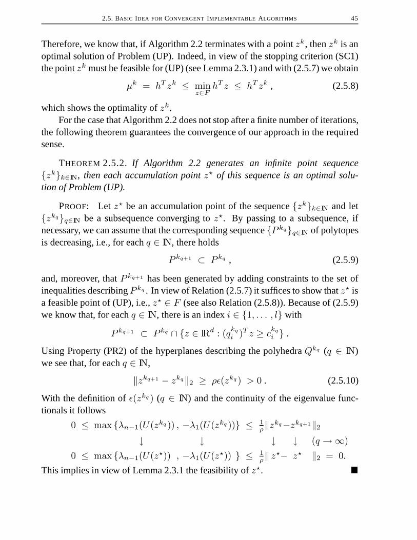
2.5. BASIC IDEA FOR CONVERGENT IMPLEMENTABLE ALGORITHMS 45
Therefore, we know that, if Algorithm 2.2 terminates with a pointzk, thenzk is anoptimal solution of Problem (UP). Indeed, in view of the stopping criterion (SC1)the pointzk must be feasible for (UP) (see Lemma 2.3.1) and with (2.5.7) we obtain
µk = hT zk ≤ minz∈F
hT z ≤ hT zk , (2.5.8)
which shows the optimality ofzk.For the case that Algorithm 2.2 does not stop after a finite number of iterations,
the following theorem guarantees the convergence of our approach in the requiredsense.
THEOREM 2.5.2. If Algorithm 2.2 generates an infinite point sequence{zk}k∈IN, then each accumulation pointz? of this sequence is an optimal solu-tion of Problem (UP).
PROOF: Let z? be an accumulation point of the sequence{zk}k∈IN and let{zkq}q∈IN be a subsequence converging toz?. By passing to a subsequence, ifnecessary, we can assume that the corresponding sequence{P kq}q∈IN of polytopesis decreasing, i.e., for eachq ∈ IN, there holds
P kq+1 ⊂ P kq , (2.5.9)
and, moreover, thatP kq+1 has been generated by adding constraints to the set ofinequalities describingP kq . In view of Relation (2.5.7) it suffices to show thatz? isa feasible point of (UP), i.e.,z? ∈ F (see also Relation (2.5.8)). Because of (2.5.9)we know that, for eachq ∈ IN, there is an indexi ∈ {1, . . . , l} with
P kq+1 ⊂ P kq ∩ {z ∈ IRd : (qkq
i )T z ≥ ckq
i } .
Using Property (PR2) of the hyperplanes describing the polyhedraQkq (q ∈ IN)we see that, for eachq ∈ IN,
‖zkq+1 − zkq‖2 ≥ ρε(zkq) > 0 . (2.5.10)
With the definition ofε(zkq) (q ∈ IN) and the continuity of the eigenvalue func-tionals it follows
0 ≤ max {λn−1(U(zkq)) , −λ1(U(zkq))} ≤ 1ρ‖zkq−zkq+1‖2
↓ ↓ ↓ ↓ (q →∞)
0 ≤ max {λn−1(U(z?)) , −λ1(U(z?)) } ≤ 1ρ‖ z?− z? ‖2 = 0.
This implies in view of Lemma 2.3.1 the feasibility ofz?. �

46 CONVERGENT OUTER APPROXIMATION ALGORITHMS FORSOLVING UNARY PROBLEMS
REMARK 2.5.2. As the previous considerations show, it is not necessary thatin the formulation of Algorithm 2.2 the numberl ∈ IN and the positive real valueρ are chosen independent of the iteration counterk. As long as there is a numberL ∈ IN with lk ≤ L (k ∈ IN) and a constantc > 0 with ρk ≥ c (k ∈ IN) thecorrectness of this solution method for (UP) can be proven.
Under the assumption that appropriate polyhedraQk (k ∈ IN) can be con-structed we have now a convergent algorithm with linear subproblems for solvingunary problems of type (UP). In order to obtain implementable algorithms we stillhave to specify, how such polyhedra can be determined. In the next section wepresent three possibilities for the choice of such sets.
2.6. Appropriate Polyhedra for Algorithm 2.2
Let zk (k ∈ IN) be the current point at iterationk of Algorithm 2.2 withε(zk) = max{λn−1(U(zk)),−λ1(U(zk))} > 0, and letBzk be the correspondingEuclidean norm ball with radiusε(zk) centered atzk. There exists of course an infi-nite number of polyhedraQk ⊂ IRd satisfying the required properties, ifρ ∈ (0, 1]andl ∈ IN are chosen accordingly. In order to obtain an efficient algorithm suchpolyhedra should satisfy some criteria apart from the necessary properties (PR1)and (PR2). First of all these sets should be easy to construct. Moreover, such apolyhedron should have as few describing hyperplanes as possible in order to re-duce the storage requirements (see Remark 2.5.1(c)). And, a third criterion is, thatthe intersection of this polyhedron with the eliminable ball should have the biggestpossible volume. Unfortunately, these criteria are conflictive. For example, theless hyperplanes we use to describe the polyhedra the less volume of the resultingintersection sets we can expect.
The first type of polyhedra, which we present in this section, is a hypercube.These sets are really easy to construct and are a relative good choice with respectto the third criterion. However, they do not pay so much attention to our secondcriterion. Therefore, we propose furthermore two possible polyhedra which baseond-simplices and are described by onlyd+ 1 respectivelyd hyperplanes, insteadof the2d hyperplanes in the case of the hypercubes. The first simplex, which wepropose in Subsection 2.6.2, is also easy to construct. In order to obtain a better setwith respect to the volume criterion we modify this simplex in Subsection 2.6.3.However, the construction of this modifiedd-simplex will need more effort.

2.6. APPROPRIATEPOLYHEDRA FOR ALGORITHM 2.2 47
2.6.1. Hypercubes.Using the fact that, for eachz ∈ IRd, there holds
‖z‖22 =d∑i=1
|zi|2 ≤d∑i=1
‖z‖2∞ = d‖z‖2∞ , (2.6.1)
we immediately see, that the`∞-norm ball centered atzk with radiusε(zk)√d
is con-
tained in the Euclidean norm ball with radiusε(zk). This`∞-norm ball is a hyper-
cube centered atzk with edge-length2 ε(zk)√d
and can be described by
Rk = {z ∈ IRd : (qki )T z ≤ cki , i = 1, . . . , 2d} (2.6.2)
where, fori = 1, . . . , d,
(qki )T z = zi and cki = zki + ε(zk)√
d,
and, fori = d+ 1, . . . , 2d,
(qki )T z = −zi−d and cki = −zki−d + ε(zk)√
d.
The hypercubesRk (k ∈ IN) fulfill Property (PR1) (see (2.6.1)) and in view of thedefinition of the hyperplanesH(qki , c
ki ) (i = 1, . . . , 2d; k ∈ IN) we know
d(zk, H(qki , cki )) =
|(qki )T zk − cki |‖qki ‖2
=1√dε(zk) .
Choosingl = 2d andρ = 1√d
in the initialization of Algorithm 2.2 the hypercube
Rk is an appropriate choice for the necessary polyhedronQk (k ∈ IN). If we applyAlgorithm 2.2 using these hypercubes for solving our example problem, then thefirst iteration of this approach looks like it is described on page 43 (see, in particular,Figure 2.4).
REMARK 2.6.1. If the hypercubesRk are used in Algorithm 2.2 forQk
(k ∈ IN), the number of inequalities describing a polytopeP ∈ P can be boundedby m + 2d. Note that the normalsqki (i = 1, . . . , 2d; k ∈ IN) of the constraintsdescribingRk do not depend on the iteration counter, and, thus, only the right-handsidescki (i = 1, . . . , 2d; k ∈ IN) of the constraints change.
The hypercubesRk (k ∈ IN) are really easy to construct and fulfill thus thepostulated first criterion. However, the number2d of generated new polytopes ineach iteration of the algorithm is already rather large. In order to reduce this numberwe develop now an inner approximation polytope for the ballBzk , which can be

48 CONVERGENT OUTER APPROXIMATION ALGORITHMS FORSOLVING UNARY PROBLEMS
described byd+ 1 hyperplanes. This choice is hence better – regarding our secondcriterion.
2.6.2. Regulard-Simplices. A d-simplex is the set among alld-dimensionalpolytopes, which can be described by the least number of linear constraints. Wepresent now ad-simplex contained in the Euclidean norm ballBzk , whose verticeslie on the boundary of this ball. It is known that among alld-simplices containedin such a ball the so-calledregular simplices, i.e., the simplices where the distancebetween each pair of vertices is equal, are the largest ones with respect to the vol-ume (see [SLE69] for a proof). In view of the third criterion we choose, therefore,a regulard-simplex contained inBzk .
In order to simplify the presentation we start with the description of a regulard-simplex centered at the origin and with vertices on the boundary of the unit ballB = {z ∈ IRd : ‖z‖2 ≤ 1}. This simplex can later be easily transformed to therequiredd-simplex lying in the relevant ballBzk .
Assume, at first, that a regulard-simplexS = [v0, . . . , vd] centered at theorigin and with all its vertices on the boundary ofB is given. Then it is knownfrom the literature that the edge-length ofS, i.e., the Euclidean distance betweeneach pair of vertices, is given by
‖vi − vj‖2 =
√2(d+ 1)
d, i, j ∈ {0, . . . , d} with i 6= j (2.6.3)
(see, e.g., [SOM29, GKL95]). Moreover, it is elementary to show that0 =1d+1
∑di=0 vi, i.e., the origin is the barycenter ofS, and that the radius of the largest
Euclidean ball, which can be inscribed intoS, is
r =1d
. (2.6.4)
The numberr is also the distance of each facet ofS to the origin. Furthermore,we can use the fact that, for eachj ∈ {0, . . . , d}, the vertexvj is orthogonal tothe facetSj = [v0, . . . , vj−1, vj+1, . . . , vd] of S, and hence the hyperplanesHSj
generated bySj can be described by
HSj = {z ∈ IRd : vTj (vi − z) = 0} (2.6.5)
with an arbitrary, but fixed indexi ∈ {0, . . . , d} \ {j}.

2.6. APPROPRIATEPOLYHEDRA FOR ALGORITHM 2.2 49
These are known results about the properties of a regulard-simplex centeredat the origin and with all its vertices on the boundary of the unit ballB. To the au-thor’s knowledge there is, unfortunately, no explicit construction of such a simplexin the literature – except of [HR98]. In order to derive an implementable algorithmwe need an explicit formulation of the hyperplanes describing such a simplex and,thus, in view of (2.6.5) we need an explicit formulation of its vertices. This will bedone in the following. For reasons which will become evident later in this sectionwe construct a regularr-simplex withr ∈ IN. Set
v0 =√a0er ,
vi =√a2ier−i −
i∑j=1
√a2j−1er−(j−1) , i = 1, . . . , r − 1 ,
vr = −√a2(r−1)e1 −r−1∑j=1
√a2j−1er−(j−1) ,
(2.6.6)
where
a0 = 1 ,
ai =
{ai−1/
(r − i−1
2
)2, if i odd
ai−2 − ai−1 , if i even, i = 1, . . . , 2(r − 1) ,
(2.6.7)
andei ∈ IRr is thei-th unit vector. Ther-simplexS = [v0, . . . , vr], which is gen-erated by these vertices, is a regular simplex with the edge-length (2.6.3), and all itsvertices belong to the boundary of the unit ballB ⊂ IRr. This will be the result ofTheorem 2.6.2. At first, however, a technical lemma is needed in order to establishthis theorem.
LEMMA 2.6.1. Letai (i ∈ {0, . . . , 2(r − 1)}) be defined as in (2.6.7). Then,for eachi = 1, . . . , r − 1, there holds
r − i+ 1r − i a2i =
r + 1r
. (2.6.8)
PROOF: We prove this result by an induction with respect toi. The assertionis obviously correct fori = 0. Assume that it holds fori = j − 1 with j ≥ 1. Then
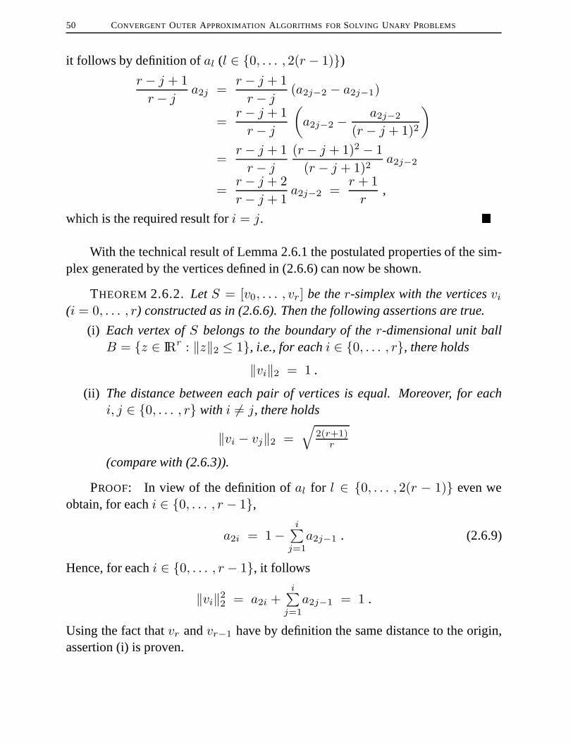
50 CONVERGENT OUTER APPROXIMATION ALGORITHMS FORSOLVING UNARY PROBLEMS
it follows by definition ofal (l ∈ {0, . . . , 2(r − 1)})r − j + 1r − j a2j =
r − j + 1r − j (a2j−2 − a2j−1)
=r − j + 1r − j
(a2j−2 − a2j−2
(r − j + 1)2
)
=r − j + 1r − j
(r − j + 1)2 − 1(r − j + 1)2
a2j−2
=r − j + 2r − j + 1
a2j−2 =r + 1r
,
which is the required result fori = j. �
With the technical result of Lemma 2.6.1 the postulated properties of the sim-plex generated by the vertices defined in (2.6.6) can now be shown.
THEOREM 2.6.2. Let S = [v0, . . . , vr] be ther-simplex with the verticesvi(i = 0, . . . , r) constructed as in (2.6.6). Then the following assertions are true.
(i) Each vertex ofS belongs to the boundary of ther-dimensional unit ballB = {z ∈ IRr : ‖z‖2 ≤ 1}, i.e., for eachi ∈ {0, . . . , r}, there holds
‖vi‖2 = 1 .
(ii) The distance between each pair of vertices is equal. Moreover, for eachi, j ∈ {0, . . . , r} with i 6= j, there holds
‖vi − vj‖2 =√
2(r+1)r
(compare with (2.6.3)).
PROOF: In view of the definition ofal for l ∈ {0, . . . , 2(r − 1)} even weobtain, for eachi ∈ {0, . . . , r − 1},
a2i = 1−i∑
j=1
a2j−1 . (2.6.9)
Hence, for eachi ∈ {0, . . . , r − 1}, it follows
‖vi‖22 = a2i +i∑
j=1
a2j−1 = 1 .
Using the fact thatvr andvr−1 have by definition the same distance to the origin,assertion (i) is proven.

2.6. APPROPRIATEPOLYHEDRA FOR ALGORITHM 2.2 51
Lemma 2.6.1 yields
‖vr−1 − vr‖22 = 4a2(r−1) = 2r − (r − 1) + 1r − (r − 1)
a2(r−1) =2(r + 1)
r,
and by using additionally (2.6.9) we obtain, fori, j ∈ {0, . . . , r} with i < j andi < r − 1,
‖vi − vj‖22 = a2j +j∑
l=i+2
a2l−1 +(√a2i +
√a2i+1
)2= 1−
j∑l=1
a2l−1 +j∑
l=i+2
a2l−1 +(√a2i +
√a2i+1
)2= 1−
i+1∑l=1
a2l−1 + a2i + a2i+1 + 2√a2i√a2i+1
= 2a2i + 2√a2i
√a2i
(r−i)2 = 2a2i + 2a2i1
r − i= 2
r − i+ 1r − i a2i =
2(r + 1)r
,
which shows assertion (ii) and completes the proof. �
As a direct consequence of the previous theorem, we obtain that the innerproduct of each pair of vertices of the simplexS = [v0, . . . , vr] is equal− 1
r .
COROLLARY 2.6.3. Under the assumptions of Theorem 2.6.2 there holds, foreachi, j ∈ {0, . . . , r} with i 6= j,
vTi vj = − 1r . (2.6.10)
PROOF: From result (ii) of Theorem 2.6.2 we know that, for eachi, j ∈ {0, . . . , r} with i 6= j, there holds
2 r+1r = ‖vi − vj‖22 = ‖vi‖22 + ‖vj‖22 − 2vTi vj .
Using assertion (i) of this theorem we obtain
2 r+1r = 2− 2vTi vj ,
which implies (2.6.10). �
In view of the previous results the construction (2.6.6) withr = d yields theneeded explicit formulation of a regulard-simplexS = [v0, . . . , vd] centered at theorigin, whose vertices lie on the boundary of the unit ball. Assume now that we are

52 CONVERGENT OUTER APPROXIMATION ALGORITHMS FORSOLVING UNARY PROBLEMS
again in the situation of Algorithm 2.2 and that a pointzk ∈ P = {z ∈ IRd : Az ≤b} is given satisfyingU(zk) /∈ Un, i.e.,
ε(zk) = max{λn−1(U(zk)),−λ1(U(zk))} > 0 .
It could be verified by straightforward calculations that the polyhedron
Sk := {z ∈ IRd : −vTi z ≤ ε(zk)d − vTi zk , i = 0, . . . , d} (2.6.11)
with vi (i = 0, . . . , d) defined as in (2.6.6) is a regulard-simplex centered atzk
(compare with (2.6.5)). The vertices ofSk areε(zk)vi + zk (i = 0, . . . , d), whichlie on the boundary of the ballBzk . For the Euclidean distance of the pointzk to thehyperplanes describingSk we obtain regarding (2.5.3), for eachi ∈ {0, . . . , d},
d(zk, H(−vi, ε(zk)d − vTi zk)) =
ε(zk)d
(2.6.12)
(compare with (2.6.4)). Thus, choosingl = d + 1 andρ = 1d in the initialization
of Algorithm 2.2, the regulard-simplicesSk are also an appropriate choice for thepolyhedraQk (k ∈ IN) needed in this approach.
REMARK 2.6.2. If the regulard-simplices defined in (2.6.11) are used in Al-gorithm 2.2 forQk (k ∈ IN), the number of inequalities describing a polytopeP ∈ P can be bounded bym + d + 1. As in the case of the hypercubes (see Re-mark 2.6.1), the normalsqki = −vi (i = 0, . . . , d; k ∈ IN) do not depend on theiteration counterk.
Example. If we choose in Algorithm 2.2 this regulard-simplex for subdivid-ing the feasible region of Problem (UPE), then we obtain in the first iteration thefollowing polytopes (see also page 43).
P 01 = P 0 ∩ {z ∈ IR2 : −z12 ≥ 1
2 + 2√
2} = ∅P 0
2 = P 0 ∩ {z ∈ IR2 : 12 (−√
3z11 + z12) ≥ 12 (1 −
√3− 2
√2)}
P 03 = P 0 ∩ {z ∈ IR2 : 1
2 (√
3z11 + z12) ≥ 12 (1 +
√3− 2
√2)}
This situation is illustrated in Figure 2.5. The new solutions are given byz02 =
(1, 1− 2√
2)T with optimal value 1√2− 1 andz0
3 = (1 + 1√3,−2√
2)T with value1√3− 1. The polytopeP 1 for iteration1 is henceP 0
3 with µ1 = −0.4226.
The presentedd-simplexSk is an inner approximation polytope for the wholeball Bzk , which can be cut out of the relevant feasible setP k. In Section 2.5 we

2.6. APPROPRIATEPOLYHEDRA FOR ALGORITHM 2.2 53
FIGURE 2.5. First iteration of Algorithm 2.2 with a regular sim-plex applied for (UPE)
z112
z12
√2
P 03−√2
P 02
S0
only require that the intersection of the polyhedronQk with P k is an inner approxi-mation of the intersection ofP k with the ballBzk . Therefore, by constructing a setbased on anotherd-simplex, which contains a bigger part ofP k∩Bzk , i.e., a biggerpart of the set which can really be eliminated, we obtain – taking our third criterionfor appropriate polyhedraQk (k ∈ IN) into account – a better choice. Note, inparticular, that all points ofP k belonging toBzk must lie in a half-ball ofBzk .
2.6.3. A Better Polyhedron Based on a Modifiedd-Simplex. The regulard-simplexSk defined in (2.6.11) does not depend on the current polytopeP k. Theconstruction of these sets only use the pointzk and the corresponding valueε(zk).In the following we present a polyhedron derived from ad-simplex, which alsorecognize the bearing of the polytopeP k with respect to the pointzk. For thisaim we need, as in Ramana’s approach (see Section 2.3), thatzk is a vertex of thecurrent polytopeP k. This is always satisfied, if we use the Simplex-Algorithm forsolving the linear subproblems in Algorithm 2.2.
Let zk be a vertex ofP k (k ∈ IN) and letBkz ≤ rk, withBk = (bk1 , . . . , bkd)T
regulard×dmatrix, be the nonsingular basic system corresponding tozk (comparewith Section 2.3, in particular page 29). Let, furthermore,
Ck = {z ∈ IRd : Bkz ≤ rk}

54 CONVERGENT OUTER APPROXIMATION ALGORITHMS FORSOLVING UNARY PROBLEMS
be the cone defined by this system. Each of thed extremal directionswki ∈ IRd
(i = 1, . . . , d) of Ck is a nontrivial solution of the system
(bkj )Twki = 0 j = 1, . . . , i− 1, i+ 1, . . . , d
(bki )Twki ≤ 0 .
Let, for i ∈ {1, . . . , d}, the vectorwki ∈ IRd denote the intersection point of theray
{z ∈ IRd : z = zk + βwki , β ≥ 0}with the boundary of the ballBzk , i.e.,
wki = zk + ε(zk) wki
‖wki‖2
(see Figure 2.6). Let, furthermore,
Hk = H(ak, bk) = {z ∈ IRd : (ak)T z = bk} (2.6.13)
with ak ∈ IRd, bk ∈ IR be the uniquely determined hyperplane containing each ofthese intersection pointswki (i = 1, . . . , d) and satisfying(ak)T zk > bk. SinceP k
is a subset ofCk and in view of the quadratic cut (2.4.6) we know that no feasiblepoint of (UP) belongs to the set
H+(ak, bk) = {z ∈ IRd : (ak)T z ≥ bk}(see again Figure 2.6). This means that the linear constraint
FIGURE 2.6. The hyperplaneH0 in the case of Problem (UPE)
������
������
(a0)T z = b0
H+(a0,b0) w01
w02z12
z11
√2
−√2
2

2.6. APPROPRIATEPOLYHEDRA FOR ALGORITHM 2.2 55
(ak)T z ≤ bk (2.6.14)
is a valid cut for (UP).
REMARK 2.6.3. The cut (2.6.14) could be used in order to derive an outerapproximation method for solving (UP), as we did in Section 2.3 with the cutsintroduced by Ramana (see Algorithm 2.1). However, since the definition ofak
(k ∈ IN) depends on the current nonsingular basic systemBkz ≤ rk correspondingto zk, such an algorithm can – similar to Ramana’s original approach – fail toconverge. Nevertheless, as we will see in Section 2.7, each known valid cut can beused for accelerating the convergence of our solution scheme for (UP).
If we take ad-simplexSk, which is the convex hull of the intersection pointak of the ray{z ∈ IRd : z = zk − βak , β ≥ 0} with the boundary ofBzk and aregular (d− 1)-simplex contained in the intersection ofHk with the ballBzk , thenwe obtainSk ⊂ Bzk ∩{z ∈ IRd : (ak)T z ≤ bk} (Sk is contained in the shaded re-gion in Figure 2.6). The polyhedronQk described by thed hyperplanes, which areinduced by just the facets ofSk containingak, obviously fulfills Property (PR1).And, moreover, we can expect that the Euclidean distance of the hyperplanes de-scribingQk to the pointzk is bigger than the distance of the facets of the regulard-simplex introduced in the previous subsection (see (2.6.11)). The two possiblechoices ofQk in Algorithm 2.2 proposed until now are fully contained in the ballBzk . The polyhedronQk, which we present below, does not have this property.Only the intersection ofQk with the current polytopeP k will be contained in thisball. Therefore, we can hope, that a bigger part ofP k is cut out of this set byapplying the polyhedronQk instead ofSk or maybe even instead ofRk.
As mentioned before, the construction of the new polyhedronQk is based ona d-simplex. Let us first describe the construction of thisd-simplex. In order tosimplify the presentation we assume again thatBzk is the unit ballB and thatHk
is a hyperplane parallel to{z ∈ IRd : zd = 0}, i.e.,Hk = H = {z ∈ IRd :−eTd z = −δ}, whereδ ∈ [0, 1) denotes the Euclidean distance ofH to the origin.After the derivation of the requiredd-simplex for this situation we describe, howthis "standard" simplex can be transformed to the general case ofBzk andHk
defined as in (2.6.13).The intersection ofH with the unit ball is a (d-1)-dimensional sphere with
radiusε =√
1− δ2 and centered atδed. Let v0, . . . , vd−1 be the vertices of aregular (d − 1)-simplex constructed as in (2.6.6). Assume that these vertices are

56 CONVERGENT OUTER APPROXIMATION ALGORITHMS FORSOLVING UNARY PROBLEMS
imbedded in the spaceIRd by adding one dimension. Set now, fori = 0, . . . , d−1,
vi := εvi + δed
andvd := ed .
It follows immediately that the verticesvi (i = 1, . . . d − 1) are contained inthe hyperplaneH . From Theorem 2.6.2 and the construction of the pointsvi(i = 0, . . . d) we see that
‖vi‖2 = 1 , i ∈ {1, . . . , d} ,
‖vi − vj‖2 = ε√
2dd−1 , i, j ∈ {0, . . . , d− 1} with i 6= j ,
‖vi − vd‖2 =√
1− δ2 + (1− δ)2 , i ∈ {0, . . . , d− 1} .
In order to use the simplexS = [v0, . . . , vd] for the construction of an ap-propriate polyhedronQk (k ∈ IN) for Algorithm 2.2, we have to derive, for eachi ∈ {0, . . . , d−1}, a representation of the hyperplanesHSi
generated by the facets
Si = [v0, . . . , vi−1, vi+1, . . . , vd]
of S. Note thatH is the hyperplane induced by the facetSd. The following lemmadelivers this representation.
LEMMA 2.6.4. Let v0, . . . , vd−1 ∈ IRd be the vertices of a regular (d − 1)-simplex defined as in (2.6.6). Set, for eachi ∈ {0, . . . , d− 1},
vi := vi − τ
d− 1ed
with
τ =√
1− δ21− δ ≥ 1 . (2.6.15)
Then, for eachi ∈ {0, . . . , d − 1}, the hyperplaneHSigenerated by the facetSi
of thed-simplexS can be described by
HSi= {z ∈ IRd : vTi z = vTi vd} . (2.6.16)
PROOF: Since, for eachi ∈ {0, . . . , d− 1}, we know
HSi= {z ∈ IRd : z = vd +
d−1∑j=0,j 6=i
γj(vj − vd) , γj ∈ IR+} ,

2.6. APPROPRIATEPOLYHEDRA FOR ALGORITHM 2.2 57
it suffices to show thatvi is orthogonal to each direction(vj−vd) (j = 0, . . . , d−1;j 6= i) of HSi
and, thus, orthogonal toHSiitself. I.e., we have to prove, for each
j ∈ {0, . . . , d− 1} \ {i},vTi (vj − vd) = 0 . (2.6.17)
Choose an arbitrary, but fixed indexj ∈ {0, . . . , d− 1} \ {i}. Applying Corollary2.6.3 and the fact that, for eachl ∈ {0, . . . , d − 1}, thed-th component ofvl iszero we obtain
vTi (vj − vd) =(vi − τ
d−1ed
)T(εvj + δed − ed)
= ε vTi vj︸︷︷︸=− 1
d−1
+(δ − 1) vTi ed︸ ︷︷ ︸=0
− ετd−1 e
Td vj︸︷︷︸=0
+ τ(1−δ)d−1 eTd ed︸︷︷︸
=1
= − εd−1 + τ(1−δ)
d−1 = 0 ,
which shows (2.6.17) and finishes the proof. �
The polyhedron, which we derive from the simplexS, will be determined bythed hyperplanes described in the last lemma. By construction we know that thispolyhedron fulfills Property (PR1). In order to guarantee that this polyhedron alsosatisfies Property (PR2) we need the Euclidean distance of the hyperplanesHSi
(i = 0, . . . , d − 1) to the pointzk, i.e., in the considered situation to the origin.Moreover, we have postulated that the polyhedron, which we develop in this sub-section, cuts a bigger part out of the unit ballB than the regulard-simplexS derivedin Subsection 2.6.2. This would be satisfied, if the distance of the hyperplanesHSi
(i = 0, . . . , d− 1) is bigger than1d (compare with (2.6.4)).
THEOREM 2.6.5. LetHSi(i = 0, . . . , d − 1) be the hyperplanes defined in
Lemma 2.6.4. Then, for eachi ∈ {0, . . . , d− 1}, the Euclidean distanced(0, HSi)
of these hyperplanes to the origin is
d(0, HSi) =
τ√(d− 1)2 + τ2
>1d
(2.6.18)
with τ given as in (2.6.15).
PROOF: From
‖vi‖22 = 1 +τ2
(d− 1)2=
(d− 1)2 + τ2
(d− 1)2
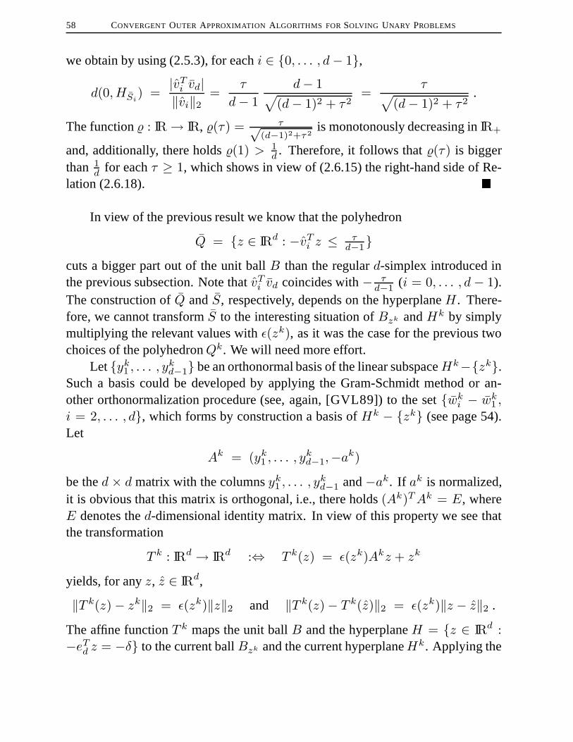
58 CONVERGENT OUTER APPROXIMATION ALGORITHMS FORSOLVING UNARY PROBLEMS
we obtain by using (2.5.3), for eachi ∈ {0, . . . , d− 1},
d(0, HSi) =
|vTi vd|‖vi‖2 =
τ
d− 1d− 1√
(d− 1)2 + τ2=
τ√(d− 1)2 + τ2
.
The function% : IR→ IR, %(τ) = τ√(d−1)2+τ2
is monotonously decreasing inIR+
and, additionally, there holds%(1) > 1d . Therefore, it follows that%(τ) is bigger
than 1d for eachτ ≥ 1, which shows in view of (2.6.15) the right-hand side of Re-
lation (2.6.18). �
In view of the previous result we know that the polyhedron
Q = {z ∈ IRd : −vTi z ≤ τd−1}
cuts a bigger part out of the unit ballB than the regulard-simplex introduced inthe previous subsection. Note thatvTi vd coincides with− τ
d−1 (i = 0, . . . , d − 1).The construction ofQ andS, respectively, depends on the hyperplaneH . There-fore, we cannot transformS to the interesting situation ofBzk andHk by simplymultiplying the relevant values withε(zk), as it was the case for the previous twochoices of the polyhedronQk. We will need more effort.
Let{yk1 , . . . , ykd−1} be an orthonormal basis of the linear subspaceHk−{zk}.Such a basis could be developed by applying the Gram-Schmidt method or an-other orthonormalization procedure (see, again, [GVL89]) to the set{wki − wk1 ,i = 2, . . . , d}, which forms by construction a basis ofHk − {zk} (see page 54).Let
Ak = (yk1 , . . . , ykd−1,−ak)
be thed × d matrix with the columnsyk1 , . . . , ykd−1 and−ak. If ak is normalized,
it is obvious that this matrix is orthogonal, i.e., there holds(Ak)TAk = E, whereE denotes thed-dimensional identity matrix. In view of this property we see thatthe transformation
T k : IRd → IRd :⇔ T k(z) = ε(zk)Akz + zk
yields, for anyz, z ∈ IRd,
‖T k(z)− zk‖2 = ε(zk)‖z‖2 and ‖T k(z)− T k(z)‖2 = ε(zk)‖z − z‖2 .
The affine functionT k maps the unit ballB and the hyperplaneH = {z ∈ IRd :−eTd z = −δ} to the current ballBzk and the current hyperplaneHk. Applying the

2.6. APPROPRIATEPOLYHEDRA FOR ALGORITHM 2.2 59
inverse function(T k)−1 we can hence transform the situation of the current itera-tion k to the just examinedstandardsituation. In order to construct the simplexSin thestandardsituation we need the Euclidean distance of the resulting hyperplane
H = {z ∈ IRd : T k(z) ∈ Hk} = {z ∈ IRd : (ak)TT k(z) = bk}to the origin. This is given by
δk =|(ak)T zk − bk|
ε(zk)(2.6.19)
(compare with (2.5.3) and note that(ak)TAk = −ed). Transforming the simplexS = [v0, . . . , vd] of thestandardsituation to the current situation in iterationk weobtain with
Sk = [T k(v0), . . . , T k(vd)]
ad-simplex contained in the set
Bzk ∩ {z ∈ IRd : (ak)T z ≤ bk} .
It can be verified by straightforward calculations that the hyperplanes inducedby the facetsSki (i = 0, . . . , d − 1) of the simplexSk containing the pointak = zk − ε(zk)ak are given by
HSki
={z ∈ IRd :
(Ak(τk
d−1ed − vi))T
(z − zk) = ε(zk)τk
d−1
}
with τk =√
1−(δk)2
1−δk and withv0, . . . , vd−1 defined as in (2.6.6) forr = d − 1.Moreover, it follows that, for eachi ∈ {0, . . . , d − 1}, the Euclidean distance ofthese hyperplanes to the pointzk is
d(zk, HSki) = ε(zk)
τk√(d− 1)2 + (τk)2
(2.6.20)
≥ ε(zk)1√
(d− 1)2 + 1.
Choosingl = d andρ = 1√(d−1)2+1
in the initialization of Algorithm 2.2 the
polyhedra
Qk = {z ∈ IRd :(Ak(τk
d−1ed − vi))T
(z − zk) ≤ ε(zk)τk
d−1 ,
i = 0, . . . , d− 1} (2.6.21)

60 CONVERGENT OUTER APPROXIMATION ALGORITHMS FORSOLVING UNARY PROBLEMS
are the third possible choice for the setsQk (k ∈ IN) needed in this approach.
Example. Consider once again Problem (UPE). The nonsingular basic
system corresponding toz0 = (1,−2√
2)T is given byB0 =( −1 0
0 −1
)and
r0 =( −12√
2
)(see page 31). For the hyperplaneH0 we obtain
H0 = {z ∈ IR2 : − 1√2z11 − 1√
2z12 = 2−
√2} .
The pointa0 is ( 1√2
+1,− 3√2)T , and the distanced0 ofH0 to the pointz0 is given
by 1√2. Thus, we haveτ0 = 1 +
√2 and using the matrixA0 = 1√
2
( −1 11 1
)the
subdivision ofP 0 leads to the two polytopes
P 01 = P 0 ∩ {z ∈ IRd : (1 +
√2)z11 + z12 ≥ 2}
P 02 = P 0 ∩ {z ∈ IRd : z11 + (1 +
√2)z12 ≥ −2−
√2}
(see Figure 2.7). The new solutions arez01 = (2,−2
√2)T with optimal value0
FIGURE 2.7. Subdivision ofP 0 with the polyhedronQ0 in Al-gorithm 2.2 applied for Problem (UPE)
z112
z12
H0
Q0
−√2
P 01
P 02
√2
andz02 = (1, 1− 2
√2)T with value 1√
2− 1. The polytopeP 1 for the next iteration
of Algorithm 2.2 is thereforeP 02 with µ1 = −0.2929.

2.7. A VARIANT OF ALGORITHM 2.2 61
Among the presented possibilities for the construction of the polyhedraQk
(k ∈ IN) for Algorithm 2.2 the last one leads to the least number of new polytopesin each iteration. However, the construction of these sets is, on the other hand,the most expensive one. Moreover, in contrast to the other two possibilities (seeRemark 2.6.1 and 2.6.2), the number of the constraints describing an elementP
of the collectionP cannot be bounded. Note that the normals of the linear con-straints determiningQk (k ∈ IN) depend on the iteration counterk. Therefore,even though the last approach leads to deeper cuts, at least in comparison to theregulard-simplex introduced in Subsection 2.6.2, it is not definitely clear, whichapproach leads to a more efficient algorithm for solving unary problems of type(UP). Before discussing the numerical performance of these three possibilities wepropose in the next section a still convergent variant of Algorithm 2.2, which doesnot need a subdivision of the current polytopeP k (k ∈ IN) in each iteration.
2.7. A Variant of Algorithm 2.2
Throughout the previous sections we proposed four possible valid linear cuts(see (2.3.3), (2.3.4), (2.3.5) and (2.6.14)) for the considered unary problem. Foran algorithm using only these cuts the convergence cannot be guaranteed. Nev-ertheless, the use of any valid cut can accelerate the convergence of Algorithm2.2. If we use in Algorithm 2.2 for the definition of the subdivision polytopesP ki(i = 1, . . . , l) also some of these cuts, then the resulting approach is of course stillconvergent. And, moreover, we can hope that this method needs less iterations forsolving (UP). For example, in Problem (UPE) the additional use of cut (2.3.5) leadsto a termination of Algorithm 2.2 after one step.
For the convergence of Algorithm 2.2 it is essential that for a decreasing se-quence{P k}k∈IN of polytopes we know that the corresponding point sequence{zk}k∈IN satisfies
‖zk+1 − zk‖2 ≥ ρε(zk) . (2.7.1)
The use of the subdivision process guarantees this property (see the necessary Prop-erty (PR2) of the hyperplanes describing the polyhedraQk). As long as this relationholds also ifP k+1 results fromP k by adding some other cuts, the convergence canbe ensured even without the subdivision ofP k.
The following algorithm uses this consideration. As long as a relation similarto (2.7.1) holds by adding only valid cuts we do not subdivide the current setP k.If this relation fails, we enforce (2.7.1) by splittingP k.

62 CONVERGENT OUTER APPROXIMATION ALGORITHMS FORSOLVING UNARY PROBLEMS
ALGORITHM 2.3 (Another Convergent Algorithm for Solving (UP) ).
InitializationChooseρ ∈ (0, 1] andl ∈ IN, and setP 0 ← {z ∈ IRd : Az ≤ b}.Solve the linear optimization problem (LP)minz∈P 0 hT z, and letz0 be an
optimal solution with optimal valueµP 0 = hT z0.
VP 0 ← {z0}, zP 0 ← z0,
µ0 ← µP 0 , P ← {P 0}, STOP← False, k ← 0
While STOP =False DoCompute the eigenvalues ofU(zk) indexed in increasing order.
If λ1(U(zk)) ≥ 0 AND λn−1(U(zk)) ≤ 0 Then (SC1)
STOP← True (zk is an optimal solution of (UP))
Elseε(zk)← max {λn−1(U(zk)),−λ1(U(zk))}Determine affine functionsi : IRd → IR (i = 1, . . . , qk ∈ IN) satisfying
`i(zk) > 0 and, for eachz ∈ P k with U(z) ∈ Un, `i(z) ≤ 0 (VCP)
P k ← P k ∩ {z ∈ IRd : li(z) ≤ 0 , i = 1, . . . , qk}If P k = ∅ ThenP ← P \ {P k}
ElseSolve the LPminz∈Pk hT z and letzk be an optimal solution.
If minz∈V
P k
{‖zk − z‖ − ρε(z)} < 0 Then (SDC)
Choosez ∈ VPk satisfying‖zk − z‖2 − ρε(z) < 0.
Construct a polyhedronQk = {z ∈ IRd : (qki )T z ≤ cki , i = 1, . . . , l}
satisfying
P k ∩Qk ⊂ P k ∩ {z ∈ IRd : ‖z − z‖2 ≤ ε(z)} (PR1)
and, for eachi ∈ {1, . . . , l},d(z, H(qki , c
ki )) = |(qk
i )T z−cki |
‖qki‖2
≥ ρε(z). (PR2)
For i = 1 To l DoP ki ← P k ∩ {z ∈ IRd : (qki )
T z ≥ cki }VPk
i← VPk \ {z}, zPk
i← zPk
If P ki 6= ∅ Then

2.7. A VARIANT OF ALGORITHM 2.2 63
Solve the LPminz∈PkihT z, and letzki be an optimal solution
with optimal valueµPki
= hT zki .P ← P ∪ {P ki }
EndIfEndForP ← P \ {P k}
ElseVPk ← VPk ∪ {zk}, zPk ← zk, µPk ← hT zk
EndIfEndIfIf P = ∅ Then (SC2)
STOP← True (P 0 ∩ {z ∈ IRd : U(z) ∈ Un} = ∅)Elseµk+1 ← minP∈P µPChooseP k+1 ∈ P andzk+1 ∈ P k+1 with µk+1 = µPk+1 = hT zk+1.
EndIfEndIfk ← k + 1
EndWhile
REMARK 2.7.1.
(a) If λ1(U(zk)) is smaller than0, we can use the cuts (2.3.4) and (2.3.5) intro-duced by Ramana. Ifλn−1(U(zk)) is greater than0, the cut (2.3.3) fulfillsthe valid cut property (VCP), and in both cases the new cut (2.6.14) pre-sented in the previous section is usable.
(b) If additional cuts satisfying (VCP) are used, then the number of inequalitiesdescribing a setP ∈ P cannot be bounded anymore. This does not dependon the used polyhedraQk (k ∈ IN) (compare with Remarks 2.6.1 and 2.6.2).
(c) If the setVPk is empty, then the subdivision criterion (SDC) is not fulfilled.By convention, there holdsminz∈∅ f(z) =∞.
(d) The valuesε(z) = max{λn−1(U(z)),−λ1(U(z))} (see (SDC)) have beencalculated for each element ofVPk (k ∈ IN) at an earlier stage of the algo-rithm.
(e) The Algorithm 2.3 does not coincide with Algorithm 3 presented in [HR98].

64 CONVERGENT OUTER APPROXIMATION ALGORITHMS FORSOLVING UNARY PROBLEMS
If Algorithm 2.3 terminates after a finite number of iterations either by detect-ing the emptiness of the feasible region of (UP) or by yielding an optimal solutionzk of this problem, then the correctness of these results follows by the same argu-mentation as in the case of Algorithm 2.2. The result of Lemma 2.5.1 is obviouslytrue also for this approach. Thus, we know that, for eachk ∈ IN, µk is a lowerbound for the optimal value of Problem (UP) (compare with (2.5.7)).
In order to guarantee the convergence of Algorithm 2.3 without a subdivisionof P k in each iterationk ∈ IN we have introduced the new setsVPk (k ∈ IN) andthe pointszPk (k ∈ IN). The subdivision criterion (SDC) shows that only suchpointszk ∈ P k are added to the setVPk , which fulfill, for eachz ∈ VPk ,
‖z − zk‖2 ≥ ρε(z) . (2.7.2)
There holds furthermore that in each iteration either a point is added toVPk or onepoint is eliminated from this set and that the elimination ofz ∈ VPk leads to asubdivision ofP k. In the elimination case it follows, moreover, that each pointcontained in a polytopeP ∈ P – P be the collection of the relevant polytopes inan iterationk ≥ k –, which is a subset ofP k must have a distance greater thanρε(z) to the pointz, i.e., fulfills (2.7.2) forz. These special properties of the setVPk enable us to prove the convergence of Algorithm 2.3. However, we will notshow the convergence of Algorithm 2.3 in the sense of Theorem 2.5.2. We provethat each accumulation pointz? of the sequence{zPk}k∈IN, which is a specialsubsequence of{zk}k∈IN, leads to a unary matrixU(z?) and is hence optimal for(UP).
For this purpose we first have to show that the elements of the sequence{zPk}k∈IN change infinitely often.
LEMMA 2.7.1. Assume that Algorithm 2.3 generates an infinite sequence{P k}k∈IN of polytopes. Let{P kq}q∈IN be a subsequence of{P k}k∈IN with theproperties that, for eachq ∈ IN, P kq+1 is a subset ofP kq and, moreover, thatP kq+1 is generated by adding linear inequalities to the list of constraints describ-ing P kq . Denote byI = {q ∈ IN : zPkq+1 6= zPkq } the set of all indicesq ∈ IN,wherezPkq is different from its successor in the sequence{zPkq }q∈IN. Then thefollowing assertions are true.
(i) The setI contains an infinite number of elements, i.e.,|I| =∞.(ii) For eachq ∈ I, there holds
‖zPkq+1 − zPkq ‖2 ≥ ρε(zPkq ) . (2.7.3)

2.7. A VARIANT OF ALGORITHM 2.2 65
PROOF: Assume, first, that the decreasing sequence{P kq}q∈IN has an addi-tional property. Let, for eachq ∈ IN, P kq+1 be adirect child of P kq , i.e., assumethat, for eachq ∈ IN, there holds
P kq+1 = P kq ∩ {z ∈ IRd : `i(z) ≤ 0 , i = 1, . . . , qkq} (2.7.4)
orP kq+1 = P kq ∩ {z ∈ IRd : `i(z) ≤ 0 , i = 1, . . . , qkq}
∩ {z ∈ IRd : (qkq
j )T z ≥ ckq
j } ,(2.7.5)
where`i : IRd → IR (i = 1, . . . , qkq ) are affine functions satisfying (VCP) withrespect tozkq andj is an element of{1, . . . , l}. In view of the definition of Algo-rithm 2.3 we know that the pointzPkq+1 is only different tozPkq , if (2.7.4) holds.
In order to prove assertion (i) assume, by contradiction, thatI contains only afinite number of elements, i.e., there is an indexq0 ∈ IN such that, for eachq ≥ q0,
zPkq = zPkq0 .
It follows thatP kq+1 results fromP kq (q ≥ q0) by adding valid cuts and executinga subdivision (see (2.7.5)). Then we obtain, for eachq ≥ q0,
|VPkq+1 | = |VPkq | − 1 .
SinceVPkq (q ∈ IN) contains only a finite number of points, this is a contradictionand proves (i), in particular, it shows thatI is not empty.
Choose next an arbitrary, but fixed indexq ∈ I. It follows thatP kq+1 is givenby (2.7.4), and, moreover, thatzPkq+1 = zkq and (SDC) is not fulfilled forzkq . Weprove now that, for eachr ∈ {0, . . . , q}, there holds
‖zPkr − zPkq+1 ‖2 ≥ ρε(zPkr ) , (2.7.6)
which is a stronger result than (2.7.3). Chooser ∈ {0, . . . , q} and letr ∈ IN, r < r
be the index such thatzPkr = zkr , i.e., zPkr was set in iterationkr. Each pointused for updatingzPk is added to the setVPk and, thus, we havezPkr ∈ VPkr+1 .We distinguish two cases.
If zPkr is still an element ofVPkq , then we obtain
0 ≤ minz∈V
Pkq
{‖z − zkq‖2 − ρε(z)} ≤ ‖zPkr − zPkq+1 ‖2 − ρε(zPkr ) ,
since the subdivision criterion (SDC) is not fulfilled forzkq . This shows (2.7.6) inthis case.

66 CONVERGENT OUTER APPROXIMATION ALGORITHMS FORSOLVING UNARY PROBLEMS
If zPkr is not an element ofVPkq , then we know that there is an indexl ∈ IN,r < l < q such thatzPkr ∈ VPkl andzPkr /∈ VPkl+1 . This implies that in iterationkl a polyhedronQkl satisfying (PR1) and (PR2) with respect toz = zPkr wasconstructed. In view of (PR2) it follows that, for eachz ∈ P kl+1 , there holds
‖z − zPkr ‖2 ≥ ρε(zPkr ) .
P kq+1 is by assumption a subset ofP kl+1 . Thus, (2.7.6) follows also in this case.Let now{P kq}q∈IN be an arbitrary sequence of polytopes with the properties
given in the formulation of the lemma. In view of (2.7.6) we know that each up-date ofzPkq+1 by zkq leads to a point, which is different from allzPkl (l ≤ q).Therefore, assertion (i) follows immediately by the facts that the special sequenceconsidered first in the present proof has this property and that{P kq}q∈IN is a sub-sequence of such a special sequence. We obtain, furthermore, that (2.7.6) implies(2.7.3). �
With the results of the previous lemma we are now able to prove the postulatedconvergence of Algorithm 2.3.
THEOREM 2.7.2. Assume that Algorithm 2.3 does not terminate after a finitenumber of iterations. Then there holds that each accumulation pointz? of thesequence{zPk}k∈IN is an optimal solution of Problem (UP).
PROOF: Let z? be an accumulation point of the sequence{zPk}k∈IN and let{zPkq }q∈IN be a subsequence converging toz?. By passing to a subsequence, ifnecessary, we can assume that the corresponding sequence{P kq}q∈IN of polytopesis decreasing and, moreover, thatP kq+1 is generated by adding linear constraints tothe list of constraints describingP kq (q ∈ IN). In view of Lemma 2.7.1(i) we can,in addition, assume that each element of the sequence{zPkq }q∈IN is different fromits successor, i.e., there holds, for eachq ∈ IN,
P kq+1 ⊂ P kq
andzPkq+1 6= zPkq .
From Relation (2.7.3) (Lemma 2.7.1(ii)) we obtain, for eachq ∈ IN,
‖zPkq+1 − zPkq ‖2 ≥ ρε(zPkq ) .
Using the definition ofε(zPkq ) (q ∈ IN) and the continuity of the eigenvalue func-tionals this relation implies, as in the proof of Theorem 2.5.2, the feasibility ofz?
2.8. COMPUTATIONAL RESULTS 67
for (UP). Furthermore, for eachq ∈ IN, we know that
hT zPkq ≤ hT zkq = µPkq = µkq ≤ minz∈F
hT z ≤ hT z? ,
whereF denotes the feasible region of(UP). This shows the optimality ofz?. NotethatzPkq is the optimal solution ofminz∈P hT z for a polytopeP ⊃ P kq . �
At first glance this convergence result is weaker than the one obtained for Al-gorithm 2.2 (see Theorem 2.5.2). We only prove the convergence of a subsequenceof {zk}k∈IN. However, a direct consequence of Lemma 2.7.1 is that at the begin-ning of an infinite number of iterations we have the situation that the current pointzk coincides with the pointzPk . In view of Theorem 2.7.2 this implies that thevalues|λ1(U(zk))| and|λn−1(U(zk))| (k ∈ IN) become arbitrarily small. Thus,Algorithm 2.3 is also well defined.
We cannot expect that either Algorithm 2.2 or Algorithm 2.3 stop with anoptimal solution of Problem (UP) after a finite number of iterations. In order toobtain finite algorithms we have to be satisfied withε-approximate solutions of thisproblem, i.e., with pointsz ∈ P satisfying
max {λn−1(U(z)),−λ1(U(z))} ≤ ε (2.7.7)
for a given toleranceε > 0. If we replace the stopping criterion (SC1) in Algorithm2.2 and in Algorithm 2.3 by
If λ1(U(zk)) ≥ −ε AND λn−1(U(zk)) ≤ ε Then , (2.7.8)
then we obtain by considering Theorem 2.5.2, respectively by taking the previousconsiderations into account, in both cases a finite approach. From this point ofview, both convergence results – Theorem 2.5.2 as well as Theorem 2.7.2 – have acomparable quality.
We finish the discussion of solution methods for unary problems of type (UP)with some numerical results. In the next section we examine, in particular, the nu-merical applicability of the presented algorithms for solving all-quadratic problemsof type (QP), since this is the main scope of this dissertation.
2.8. Computational Results
Algorithm 2.3 was encoded in C++ with management of the collectionP ofrelevant polytopes by so-called AVL-trees. The linear subproblems were solved by

68 CONVERGENT OUTER APPROXIMATION ALGORITHMS FORSOLVING UNARY PROBLEMS
using the Simplex-Algorithm basedCPLEX-5.0 code. After solving the first LP-relaxation of (UP) in the initialization phase of Algorithm 2.3 each new subproblemresults from a previous one by adding some new constraints or by changing someright-hand sides. For that reason we solved only the initial problem by applying theprimal Simplex-Algorithm. The solution of each subsequent subproblem was de-termined with the dual Simplex-Algorithm, which is supported by theCPLEX-5.0code. This strategy reduced the running-time for solving the subproblems. How-ever, on the other hand, we needed more storage, since all necessary informationabout the current solution, like the dual variables, the slacks and so on, had to bestored for each polytopeP ∈ P . Otherwise, we would not be able to start the dualversion of the Simplex-Algorithm without additional effort.
Apart from the solution of linear optimization problems, other classical prob-lems can occur in Algorithm 2.3. First of all, we have to calculate eigenvalues ofdifferent matrices. For the construction of the cuts introduced by Ramana we haveto determine the inverse of a matrix (see Section 2.3). In order to obtain a repre-sentation of the polyhedraQk (k ∈ IN) (see Subsection 2.6.3) we need solutionsof linear equations and we need an orthonormal basis describing the linear spaceHk−{zk}. In the implementation of the algorithm all these problems were solvedby applying appropriate routines from theNAG C-library.
With respect to the choice of possible linear constraints satisfying the valid cutproperty (VCP) and in view of the three types of polyhedraQk (k ∈ IN) proposedin Section 2.6 there is a large number of implementable variants of Algorithm 2.3.Before discussing the numerical performance of some selected variants we presenta slight modification of the subdivision process, which can lead to a substantialimprovement of the numerical performance of our approach.
2.8.1. A Slight Modification of the Subdivision Process.In the subdivisionprocess in Algorithm 2.3 we construct each new polytopeP ki (i = 1, . . . , l; k ∈ IN)by adding one of the constraints describingQk to the list of constraints describingP k. Independent of the choice of the polyhedronQk this strategy can lead tooverlapping regions, i.e., there can hold
intP ki ∩ intP kj 6= ∅for somei, j ∈ {1, . . . , l} (see the Figures 2.4, 2.5 and 2.7). This is not reasonable,since parts of the feasible region of (UP) are examined more than once by using thisstrategy. For the correctness of Algorithm 2.3 and Algorithm 2.2, respectively, it

2.8. COMPUTATIONAL RESULTS 69
is sufficient, if the new polytopesP ki (i = 1, . . . , l) form a partition of the setP k \ {z ∈ IRd : (qki )
T z < cki , i = 1, . . . , l}, i.e., if there holds
l⋃i=1
P ki = P k \ {z ∈ IRd : (qki )T z < cki , i = 1, . . . , l} ⊃ P k \Bzk
and, for eachi, j ∈ {1, . . . , l} with i 6= j,
intP ki ∩ intP kj = ∅ (2.8.1)
(see Definition 1.2.1). Property (2.8.1) can be achieved by a slight modification ofthe definition of the polytopesP ki . If we set, for each indexi ∈ {1, . . . , l},
P ki ← P k ∩ {z ∈ IRd : (qki )T z ≥ cki , (qkj )
T z ≤ ckj , j = 1, . . . , i− 1} ,
then we obtain that the union of the setsP ki (i = 1, . . . , l) is the same set as by onlyadding the constraint(qki )
T z ≥ cki . And, moreover, these sets fulfill the additionalproperty (2.8.1) (see Figure 2.8). In Remark 2.6.1 and Remark 2.6.2 we pointed outthat the normals of the hyperplanes describing the hypercubesRk and the regulard-simplicesSk, respectively, do not depend on the iteration counterk. Thus, if one ofthese two sets is used in Algorithm 2.3 for the polyhedronQk, the subdivision ofP k
leads only to a change of the right-hand sides of some constraints. Therefore, theproposed modification is – from a numerical point of view – not expensive and doesnot lead to new storage requirements. It does not really matter whether one right-hand side is changed or up to2d. In the case of the third presented polyhedron thisnew subdivision strategy leads to growing storage requirements and is numericallymore expensive, since the number of constraints describing a polytopeP ∈ P isgrowing faster. However, in each case we can expect that the elimination of theoverlapping parts results in a more efficient approach for solving (UP).
We applied Algorithm 2.2, i.e., Algorithm 2.3 without additional cuts, for solv-ing our example problem, where we used the subdivision process with and withoutthe modification. If we used the hypercubesRk or the polyhedronQk based on themodifiedd-simplex, then in both cases the algorithm needed the same number of it-erations and the same number of linear subproblems had to be solved. For these twocases the modification led only to a slight increase in the running-time, especiallyin the case ofQk. Note that by adding more than one constraint in an iteration theeffort for solving the resulting linear subproblems increases faster than by addingonly one constraint. Table 2.1 shows the effort for solving (UPE) with these twochoices of the polyhedronQk. The execution of Algorithm 2.2 was terminated,

70 CONVERGENT OUTER APPROXIMATION ALGORITHMS FORSOLVING UNARY PROBLEMS
FIGURE 2.8. Modification of the subdivision process applied for (UPE)
z112
z12
P 03
P 01
−√2
√2
R0
(a) HypercubeR0 (comparewith Figure 2.4)
z112
z12
S0
−√2
√2 P 0
2
P 03
(b) Regular 2-simplex S0
(compare with Figure 2.5)
z112
Q0
H0
P 02
√2
−√2
z12
P 01
(c) Better polyhedronQ0 (comparewith Figure 2.7)
if the ε-approximate stopping criterion (2.7.8) withε = 10−4 was satisfied. Thefourth column of this table showing the maximal number of polytopes, which hadto be stored at an iteration of Algorithm 2.2 in the setP , illustrates the storagerequirements of the different approaches.

2.8. COMPUTATIONAL RESULTS 71
TABLE 2.1. Effort for solving (UPE) with Algorithm 2.2
PolyhedronQk Number of Number of Maximal number Timea b
iterations solved LP’s of elements inP (in sec.)Rk 27 71 28 0.18 (0.18)Qk 16 33 17 0.17 (0.18)
arun on aSUN SPARC 20workstationbrunning-time for Algorithm 2.2 with modification is given in brackets
That the modification of the subdivision process in Algorithm 2.2 does notresult in an improvement, if we use the hypercubeRk or the polyhedronQk, de-pends on the special structure of Problem (UPE). An examination of the iterationsof Algorithm 2.2 without the modification shows that each optimal solutionzk ofa linear subproblem does not belong to a part of the current polytopeP k, whichcould be eliminated at an earlier stage of the method by applying the modification.Therefore, as well with as without the modification, the same work has to be donein order to solve Problem (UPE).
If we apply the regulard-simplexSk, the numerical performance depends sig-nificantly on the subdivision strategy used in Algorithm 2.2, as it is displayed inTable 2.2. In view of the first iteration of Algorithm 2.2 with the polyhedron
TABLE 2.2. Effort for solving (UPE) by applyingSk
Subdivision Number of Number of Maximal number Timea
strategy iterations solved LP’s of elements inP (in sec.)no modification 1708 5125 1709 16.09
modification 68 183 47 0.56
arun on aSUN SPARC 20workstation
Sk this result is not surprising. In Figure 2.5 we see that the optimal solutionz? = (1,−√2)T belongs to the two non-empty polytopesP 0
2 andP 03 . Therefore,
we know that Algorithm 2.2 without the modified subdivision strategy must gener-ate at least two sequences of polytopes{P kq}q∈IN, one starting withP 0
2 and onestarting withP 0
3 , such that the corresponding point sequences{zPkq }q∈IN convergeto z?. If we apply the modification,z? is contained in only one polytope (see Figure2.8(b)).

72 CONVERGENT OUTER APPROXIMATION ALGORITHMS FORSOLVING UNARY PROBLEMS
Taking the large performance difference of Algorithm 2.2 with and withoutthe modification in the above case into account, we can expect that on average themodification of the subdivision strategy results in an improvement of the numeri-cal performance. The extra work we have to do, especially in the case ofQk, canlead to a substantial reduction of the number of iterations and, hence, of the totaltime for solving unary problems. For that reason we examine in the next subsec-tion the numerical performance only of variants of Algorithm 2.3, which apply thedescribed modification of the subdivision strategy.
2.8.2. Applicability to All-Quadratic Problems. In the following we dis-cuss the numerical applicability of Algorithm 2.3 to all-quadratic problems of type(QP). We saw in Section 2.2 that for each problem of type (QP) there is an equiv-alent unary problem of type (UP), and, thus, we can solve arbitrary all-quadraticproblems by applying the approaches presented so far. We tried to solve the unaryproblems, which result from the previously described transformation (see Section2.2) of the all-quadratic problems belonging to our randomly generated test set (seeSection 1.5).
At the end of Section 2.7 we pointed out that we have to be satisfied withε-approximate solutions in order to obtain a finite algorithm. Theε-approximatestopping criterion (2.7.8) is usable for arbitrary unary problems. However, if weapply this stopping criterion, we know nothing about the quality of the determinedsolutionzk, in particular, we do not know how far away from the optimal value liesthe calculated valueµk = hT zk. If we solve the transformations of all-quadraticproblems, we are able to formulate a stopping criterion such that this quality ofthe determined solution with respect to the original quadratic problem can be es-timated. Before discussing the numerical performance of our approaches, we pro-pose first this special stopping criterion.
Assume that an all-quadratic problem of type (QP), i.e., a problem with theform
min xTQ0x+ (d0)Tx
xTQlx+ (dl)Tx+ cl ≤ 0 l = 1, . . . , p
AQx ≤ bQ
lQ ≤ x ≤ LQx ∈ IRn
(QP)
is given.

2.8. COMPUTATIONAL RESULTS 73
Let, furthermore,
min hT z
AUz ≤ bU
lU ≤ z ≤ LU
U(z) ∈ Un+1 , z ∈ IR(
n+12
)+n
(UP)
be the equivalent unary problem resulting from the transformation of (QP) de-scribed in Section 2.2. The superscriptsU andQ respectively are used in the sameway as in Section 2.2, and the dimensions of all involved matrices and vectors arethe same as there (see, in particular, pages 23f.).
Set
δ := min { 1‖h‖2 ,
1‖aUl ‖2
, l = 1, . . . , p} ε , (2.8.2)
whereε is a given tolerance greater than0, andaUl (l = 1, . . . , p) denotes thel-throw of the matrixAU . Let zk (k ∈ IN) be the current point at the beginning ofiterationk of Algorithm 2.3. Determine ann-dimensional pointxk by setting
xki := 1√2zki,n+1 (2.8.3)
(compare with the definition ofx in Theorem 2.2.1). Ifzk is feasible for (UP), thenwe know by the same arguments as in the proof of Theorem 2.2.1 thatxk must befeasible for (QP). Determine, furthermore, a (d =
(n+1
2
)+ n)-dimensional point
zk indexed in the same manner aszk by setting
zki,n+1 :=√
2xki , zkii := (xki )
2 (i = 1, . . . , n) ,
zkij :=√
2xki xkj (1 ≤ i < j ≤ n)
(2.8.4)
(compare with the definition ofz in Theorem 2.2.1). Ifxk is feasible for (QP),we know (see again the proof of Theorem 2.2.1) thatzk is feasible for (UP), and,moreover, that the pointszk and zk coincide. If we replace theε-approximatestopping criterion (2.7.8) by the following
If ‖zk − zk‖ ≤ δ Then (2.8.5)
with δ defined as in (2.8.2), then we obtain a solution method for all-quadraticproblems, which detects in finite time either the emptiness of the feasible region

74 CONVERGENT OUTER APPROXIMATION ALGORITHMS FORSOLVING UNARY PROBLEMS
of (QP), or delivers a pointzk such that the corresponding pointxk defined as in(2.8.3) has the properties
(xk)TQlxk + (dl)Txk + cl ≤ ε l = 1, . . . , p
AQx ≤ bQ
lQ ≤ x ≤ LQ .
(2.8.6)
If this pointxk is additionally feasible for (QP), it even follows, that the calculatedvalueµk and the optimal value of (QP) have a distance not bigger thanε.
Indeed, by replacing the stopping criterion (2.7.8) with (2.8.5) the resultingalgorithm is, first of all, still well defined. In view of Theorem 2.7.2 we knowthat each accumulation pointz? of the sequence{zPk}k∈IN is a feasible point for(UP). Thus,z? defined as in (2.8.4) is equal toz?. As mentioned at the end of theprevious section we know, furthermore, that in an infinite number of iterations thereholds that the pointszk andzPk coincide. Therefore, we achieve that the Euclideandistance betweenzk andzk becomes arbitrarily small, i.e, (2.8.5) will be fulfilledafter a finite number of iterations.
If Algorithm 2.2 or Algorithm 2.3 detects the emptiness of the feasible regionof (UP), then the emptiness of the feasible set of (QP) follows by the equivalencebetween both problems. If one of these algorithms terminates with a pointzk sat-isfying (2.8.5), it is clear thatxk defined as in (2.8.3) fulfills the linear constraintsof (QP). This follows by the construction ofAU , bU , lU andLU . Moreover, bythe special definition ofzk we achieve, as in the proof of Theorem 2.2.1, that thereholds
(xk)TQlxk + (dl)Txk + cl = (aUl )T zk − bUl l = 1, . . . , p (2.8.7)and
(xk)TQ0xk + (d0)Txk = hT zk . (2.8.8)
The relation (2.8.7) and the feasibility ofzk with respect to the linear constraints of(UP) imply, for eachl ∈ {1, . . . , p},
(xk)TQlxk + (dl)Txk + cl ≤ (aUl )T (zk − zk) ≤ ‖aUl ‖2‖zk − zk‖2 ≤ ε .
Hence,xk fulfills (2.8.6). If xk is additionally feasible for (QP), it follows with(2.8.8)
|hT zk − (xk)TQ0xk − (d0)Txk| ≤ ‖h‖2‖zk − zk‖2 ≤ ε

2.8. COMPUTATIONAL RESULTS 75
and
hT zk = µk ≤ minz∈FU
hT z ≤ hT zk = (xk)TQ0xk + (d0)Txk ,
whereFU denotes the feasible region of (UP). This means thatxk is ε-optimal forProblem (QP). With the foregoing considerations we have shown that the stoppingcriterion (2.8.5) is a more reasonable criterion than (2.7.8), when we solve all-quadratic problems of type (QP) via unary problems. If we use (2.8.5), then weknow something about the quality of the calculated pointxk with respect to thequadratic problem, which we would like to solve.
REMARK 2.8.1. The pointzk (k ∈ IN) defined as in (2.8.4) leads to a unarymatrix U(zk). Therefore, we know taking Lemma 2.3.1 and Theorem 2.4.4 intoaccount that there holds
max {λn−1(U(zk)),−λ1(U(zk))} ≤ ‖zk − zk‖2 .
This shows that with respect to the definition ofδ we need, in comparison withthe stopping criterion (2.7.8), a higher accuracy for the valuesλn−1(U(zk)) andλ1(U(zk)) in order to satisfy (2.8.5).
Our main motivation for considering unary problems were the results of Ra-mana’s dissertation [RAM 93, Chapter 7], in particular, his really promising pre-liminary numerical results. He solved with Algorithm 2.1 large unary problemswith acceptable running-times. However, the affine functionU : IRd → Sn,which he used, had a simple structure. By applying Algorithm 2.1 for solvingunary problems, which result from the transformation of all-quadratic problemsand which, thus, have a complex affine function, this pure outer approximation ap-proach showed a really bad performance in our computational tests. Even smallunary problems resulting from2-dimensional quadratic problems could not besolved in acceptable times. Moreover, this approach induced numerical problems.In many test problems the algorithm seemed to stick in a point away from anε-approximate solution. Since the hyperplanes used in this scheme became tooflatthe algorithm made small progress and the numerical problems increased. Notethat tooflat hyperplanes can lead to ill-conditioned matricesBk such that we canobtain increasing numerical errors, if we do not invest additional effort.
Even though an algorithm based only on the cuts introduced by Ramana showeda bad performance, his linear constraints can be used in Algorithm 2.3 in order toaccelerate the convergence of this approach. The fact that the use of additional cuts

76 CONVERGENT OUTER APPROXIMATION ALGORITHMS FORSOLVING UNARY PROBLEMS
in Algorithm 2.3 led to a more efficient solution method for unary problems, wasthe first result of our numerical tests. We compared different combinations of thefour valid cuts presented in this chapter. The new cut (2.6.14) did not acceleratethe convergence of Algorithm 2.3 in the most cases, when we used the cuts (2.3.3)and (2.3.5). The cut (2.3.5) was mostly better than (2.3.4). Consequently, the mostefficient combination of the possible four cuts in our numerical tests was the cut(2.3.3) for the caseλn−1(U(zk)) > 0 and (2.3.5) forλ1(U(zk)) < 0.
In the following we compare the numerical performance of Algorithm 2.3 ap-plying these two cuts with the numerical performance of Algorithm 2.2, i.e., ofAlgorithm 2.3 without any additional valid cut. In both approaches we used the hy-percubesRk developed in Subsection 2.6.1 for subdividing the setP k, if necessary.The execution of the algorithms was terminated, if the appropriate stopping crite-rion (2.8.5) was satisfied withδ defined as in (2.8.2) for a prespecified toleranceε > 0. Remember that the all-quadratic problems belonging to our test set havealways a non-empty feasible region (see Section 1.5). In order to avoid excessivestorage requirements, and, thus, also in order to avoid excessive running-times werestricted the maximal number of polytopesP , which had to be stored at an iter-ation in the collectionP . In the case of Algorithm 2.2 this maximal number was100, 000. Since the storage requirements increase, when additional cuts are used,we reduced this number to50, 000 in the case of Algorithm 2.3.
TABLE 2.3. Comparison of the numerical effort for solving2-dimensional all-quadratic problems with the accuracyε = 0.1
Algorithm NuP ANuLP MNuLP ATime MTime ACol MColp = 1
2.2 42 142,377 52,224 103.5 38.7 24,853 18,4992.3 50 26,914 1,304 96.9 2.63 2,931 404
p = 2
2.2 42 148,956 66,168 123.9 51.7 24,708 18,9012.3 50 14,015 497.5 51.9 1.08 1,235 145
p = 3
2.2 42 98,574 95,566 83.9 79.1 23,724 19,0342.3 50 4,787 746.5 12.2 1.54 789 199.5
p = 4
2.2 41 121,551 72,285 102.8 61.1 25,688 17,7442.3 50 7,423 1,398 19.5 2.96 1,038 294

2.8. COMPUTATIONAL RESULTS 77
Table 2.3 and Table 2.4 display the numerical effort, which the two describedapproaches needed in order to solve the50 5-dimensional unary problems resultingfrom the transformation of our2-dimensional quadratic test problems. We usethe abbreviations NuP for the number of test problems, which could be solvedby the two methods within the given storage capacities. ANuLP is used for theaverage number of linear problems, which had to be solved during the execution ofeach algorithm. ATime stands for the average running-time in seconds, and in thecolumn ACol we display the average maximal number of elements, which had tobe stored in the collectionP . The three columns with MNuLP, MTime and MColshow the corresponding values of the medians. Note that in the calculation of theaverage values and of the medians we considered only the problems, which couldbe solved within the given storage capacities. All numerical test discussed here,were run on aSUN ULTRA 60 workstation.
TABLE 2.4. Comparison of the numerical effort for solving2-dimensional all-quadratic problems with the accuracyε = 0.01
Algorithm NuP ANuLP MNuLP ATime MTime ACol MColp = 1
2.2 34 225,822 108,570 157.2 86.4 34,896 34,7492.3 49 56,341 2,841 197.5 6.6 5,555 768
p = 2
2.2 36 173,958 138,446 143.5 109.8 34,656 34,6072.3 49 14,699 1,007 49.0 2.11 1,473 260
p = 3
2.2 32 204,578 163,942 175.2 139.3 40,597 40,3612.3 50 11,920 1,752 35.2 3.51 1,954 401.5
p = 4
2.2 30 150,128 126,474 131.1 110.4 32,695 32,7622.3 50 17,351 2,725 53.8 6.10 2,505 532
It is obvious that Algorithm 2.3 with the additional cuts is the more efficientapproach for determiningε-approximate solutions for our test problems. In almostall cases this approach was significantly faster and, moreover, with this algorithmwe were able to solve the most problems within the given storage capacities. Algo-rithm 2.2 did not terminate with a solution in one third of the test problems, if anaccuracy ofε = 0.01 was required. In both approaches there is a great difference

78 CONVERGENT OUTER APPROXIMATION ALGORITHMS FORSOLVING UNARY PROBLEMS
between the average values and the medians. This makes clear – even though theseapproaches, in particular Algorithm 2.3, showed a rather good performance in atleast50% of the solved test examples (see the medians) – there were some exam-ples, where we needed a huge effort in order to determine a solution. Thus, ourapproach did not show a good performance on average, particularly in comparisonwith the simplicial branch-and-boundmethod for all-quadratic problems, which wewill develop in the next chapter.
An advantage of the presented approach is that the solution effort does notdepend on the numberp of quadratic constraints, as it will be the case for themethod described in the next chapter. This is due to the fact that the effort forsolving a unary problem does not depend on the number of linear constraints. Thestructure of the affine matrix mapping is decisive.
Another interesting result of our numerical tests was that the subdivision pro-cess used in Algorithm 2.3 had a regularization effect in the following sense. Wehave mentioned that Algorithm 2.1 can lead to numerical problems, if the hyper-planes used there get tooflat. In Algorithm 2.3 we used the same constructionrule for the additional cuts, but the subdivision of the current polytopeP k, whichwas enforced, if the additional cuts became tooshallow, avoided such numericalproblems. From this point of view, Algorithm 2.3 was numerically more stable.
We have seen that the additional use of valid cuts in Algorithm 2.3 is reason-able, since we obtain a significant speedup of our solution method. Our numericalexperience also showed, that on average the additional cuts (2.3.4) and (2.6.14)only increased the running-time of Algorithm 2.3. It is hence not cogent that eachaffine function satisfying (VCP) accelerate the convergence of this approach. Anappropriate combination of valid cuts is decisive. This should be considered, whennew cuts are developed in order to improve the performance of Algorithm 2.3.
We still have to examine, which choice of the polyhedronQk leads to themost efficient algorithm. For this aim we also tried to solve the2-dimensional all-quadratic test problems using the regulard-simplexSk and using the polyhedronQk. The corresponding results together with the effort of Algorithm 2.3 usingthe hypercubesRk are presented in Table 2.5 and Table 2.6. We use the sameabbreviations as in the foregoing tables. The additional columns ACon and MCondisplay the average and the median of the maximal number of linear constraints,which were needed for describing an elementP of P . These facts together withthe columns corresponding to the maximal number of elements contained inPgive us more insight into the real storage requirements. The more constraints we

2.8. COMPUTATIONAL RESULTS 79
TABLE 2.5. Comparison of the numerical effort for solving2-dimensional all-quadratic problems with the accuracyε = 0.1
Qk NuP ANuLP MNuLP ATime MTime ACol MCol ACon MConp = 1Rk 50 26,914 1,340 96.9 2.63 2,931 404 61 54Sk 45 37,721 2,2237 266 9.36 2,578 323 151 164Qk 46 27,273 2,980 226 13.42 3,226 643 159 156
p = 2
Rk 50 14,015 497.5 51.9 1.08 1,235 145 54 43.5Sk 48 12,612 814.5 89.5 3.09 1,034 147.5 132.6 113.5Qk 49 15,421 1,176 133 4.11 1,631 300 146 111
p = 3
Rk 50 4,787 746.5 12.2 1.54 789 199.5 49 50.5Sk 50 13,622 1530 98.8 5.74 1,343 193.5 134 126.5Qk 50 11,756 1,319 80.3 5.28 1,689 299 124 126
p = 4
Rk 50 7,423 1,398 19.5 2.96 1,038 294 58 56Sk 49 14,796 1,804 93.8 8.08 1,522 330 154 149Qk 50 14,668 1,915 96.4 8.44 1,963 341 155 161
need for the description of a polytopeP the more storage is used by this set. Asin the runs of Algorithm 2.3 using the hypercubesRk, we restricted the maximalnumber of elements belonging toP . By applyingSk or Qk we useρ = 1
d orρ = 1√
(d−1)2+1in the subdivision criterion (SDC). These numbers are smaller
than 1√d, which is used forρ in the case ofRk. Thus, we know that subdivisions
are more rarely enforced and that the number of constraints describing an elementof P and consequently the storage size of such an element can increase faster. Forthat reason we restricted the maximal number of polytopes inP to 20, 000, whenusing the regulard-simplexSk or the polyhedronQk in Algorithm 2.3.
The numerical results presented in the Tables 2.5 and 2.6 definitely show thatAlgorithm 2.3 using the hypercubesRk is more efficient than the same approachusingSk or Qk, at least with respect to our test problems. This seems to depend onthe fact that by usingRk a bigger part of the current polytopeP k can be eliminated.Note that the volume ofRk ⊂ IRd is given by
V (Rk) =(ε(zk)2√
d
)d=(ε(zk)√d
)d2d ,

80 CONVERGENT OUTER APPROXIMATION ALGORITHMS FORSOLVING UNARY PROBLEMS
TABLE 2.6. Comparison of the numerical effort for solving2-dimensional all-quadratic problems with the accuracyε = 0.01
Qk NuP ANuLP MNuLP ATime MTime ACol MCol ACon MConp = 1Rk 49 56,341 2,841 197.5 6.60 5,555 768 74 71Sk 40 45,923 2,600 372.4 13.5 2,632 458.5 167 170.5Qk 40 28,680 3,501 261.6 17.3 3,178 807 174 174.5
p = 2
Rk 49 14,699 1,007 49.0 2.11 1,473 260 64 55Sk 48 26,494 2,209 221.6 8.56 2,010 343 168 144Qk 48 25,035 2,645 149.8 10.94 2,578 491 191 150.5
p = 3
Rk 50 11,920 1,752 35.2 3.51 1,954 401.5 64 62Sk 48 22,820 2,930 177.2 12.0 2,441 393.5 160 165.5Qk 48 18,217 2,088 135.9 9.54 2,764 457 163 173.5
p = 4
Rk 50 17,351 2,725 53.8 6.10 2,505 532 75 72.5Sk 47 25,994 3,801 207.7 16.2 2,805 554 192 195Qk 47 22,226 4,382 191.7 25.5 3,114 809 201 213
whereas the volume of the regulard-simplexSk is
V (Sk) =√d+ 1d!
(ε(zk)
√d+ 1d
)d=(ε(zk)√d
)d (√d+ 1)d+1
d!
(see, e.g., [GKL95]). This implies that the volume ofSk is smaller thanV (Rk)and, moreover, thatV (Sk) is decreasing faster with respect to the dimensiond
thanV (Rk). The advantage of the larger volume ofRk seems to be greater thanthe disadvantage of the higher number of hyperplanes, which are necessary fordescribingRk.
Whether the use of the regular simplexSk or the use of the theoretically betterpolyhedronQk (see Theorem 2.6.5) leads to a more efficient approach cannot beanswered definitely. Even though Algorithm 2.3 usingQk was always faster on av-erage – except forp = 2 andε = 0.1 – a comparison of the corresponding mediansdoes not show a unique result. The same is true for the number of subproblems,which had to be solved during the execution of our method. Note that the averagevalues as well as the medians were calculated with respect to the number of solvedproblems. Thus, these values are not directly comparable, when different numbersof problems were solved. For example, in the casep = 4 andε = 0.1 (see Table
2.8. COMPUTATIONAL RESULTS 81
2.5) we obtain forQk an average number of11, 743 LP’s and an average running-time of76.13, considering only the49 test problems, which were also solved withSk.
With respect to the storage requirements we see that Algorithm 2.3 usingSk isa better solution scheme. We needed less polytopesP and we needed additionallyless constraints for describing these sets. Note that by usingSk and the correspond-ing value forρ the subdivision criterion (SDC) is more seldomly satisfied, such thatless splittings ofP k are necessary. Note, furthermore, that by usingQk the numberof constraints determining a polytopeP k increases also ifP k is subdivided. ByusingRk andSk this number only grows, when the additional cuts are used (seeRemark 2.6.1 and Remark 2.6.2).
UsingSk andQk the numerical results show again a high difference betweenthe average values and the medians. The reason is the same as in the case ofRk.In at least50% of the test problems both approaches showed an acceptable per-formance. However, there were numerical outliers, which destroyed the averageperformance of our algorithm. In view of the presented computational results wehave to recognize that the use of the polyhedraQk did not have the expected suc-cess. The extra work for determining a better inner approximation polytope for theeliminable part ofP k did not result in a substantial improvement of the numericalperformance of Algorithm 2.3. The easiest set, i.e., the hypercubeRk, showed thebest numerical results.
Comparing the presented results with the numerical performance of the solu-tion method for (QP), which we develop in the next chapter, Algorithm 2.3 is –even withRk – not a good approach for solving all-quadratic problems. For an ac-curacy ofε = 0.01 and quadratic problems of sizen = 2 andp = 4 we needed onaverage53.8 seconds. This bad performance boosted, if we tried to solve higher di-mensional problems. In Figure 2.9 the numbers of the3-dimensional all-quadraticproblems are displayed, which could not be solved within the given storage capac-ities by Algorithm 2.3 using the three discussed possibilities forQk and the pooraccuracyε = 0.5. The transformed unary problems had the dimension9. There-fore, we reduced the maximal number of polytopes, which could belong to the setP . When usingRk, we allowed20, 000 elements. In the cases ofSk andQk werestricted this number to10, 000. The corresponding minimal running-times, i.e.,the fastest time after which Algorithm 2.3 was terminated since the storage capac-ity was exceeded, are given in seconds in Table 2.7. Considering this table it isnot reasonable to increase the storage capacities in order to solve more problems.

82 CONVERGENT OUTER APPROXIMATION ALGORITHMS FORSOLVING UNARY PROBLEMS
FIGURE 2.9. Number of3-dimensional all-quadratic test prob-lems where Algorithm 2.3 exceeded the given storage capacity
65
43
21
0
5
10
15
20
25
30
35
40
45
50
Number of quadratic constraints
Sk
Rk
Qk
usedpolyhedron
TABLE 2.7. Minimal running-times of unsolved3-dimensionalall-quadratic problems withε = 0.5
p = 1 p = 2 p = 3 p = 4 p = 5 p = 6Rk 125.9 122.2 139.9 147.2 303.8 433.7Sk 503.6 473.1 440.4 431.8 549.4 586.9Qk 280.1 334.5 301.2 321.7 348.3 414.5
A running-time of at least2 minutes for one of the still unsolved3-dimensionalquadratic test problems is indeed not acceptable.
The last computational results demonstrate the, maybe, biggest disadvantageof the attempt to solve all-quadratic problems of type (QP) via unary problems. Thetransformation of the quadratic problems leads to anexplosionof the dimensionof the resulting (UP). Even for a3-dimensional (QP) we obtain a9-dimensionalunary problem. If we recognize, furthermore, that the numerical applicability ofgeneral global optimization methods based on cutting planes or on branch-and-bound techniques is limited to problems in small spaces, it is not surprising thatAlgorithm 2.3 is not able to solve all-quadratic problems in dimensions higher than

2.8. COMPUTATIONAL RESULTS 83
3, at least that Algorithm 2.3 is not able to solve such problems with acceptableeffort.
Algorithm 2.3 has still a lot of features, which could be changed. We could tryto develop new valid cuts. We could use other values ofρ in (SDC) (see Remark2.5.2) in order to change the number of subdivisions or instead we could look forother polyhedra. Nevertheless, in view of the previous considerations, it is unlikelythat the solution of all-quadratic problems by using unary problems is a practicableway. In the next chapter we will see that a direct solution method for all-quadraticproblems can have a significantly better numerical performance.

84 CONVERGENT OUTER APPROXIMATION ALGORITHMS FORSOLVING UNARY PROBLEMS

CHAPTER 3
A Simplicial Branch-and-Bound Method for SolvingNonconvex All-Quadratic Problems
In this chapter we will discuss a direct approach for solving nonconvexall-quadraticproblems of type (QP). In the introduction (see Section 1.3) we pointed out that themost solution approaches for Problem (QP) proposed in the literature were devel-oped for more general problem classes containing (QP) as a special instance. To theauthor’s knowledge there is up to now only one approach considering directly thegeneral nonconvex all-quadratic problem. This approach presented by Al-Khayyalet al. [AKLV95] is a rectangular branch-and-bound scheme.
The simplicial branch-and-bound method for solving (QP), which we will in-troduce and examine throughout the present chapter, use the same basic conceptsas this rectangular scheme. This new solution method shows a significantly bet-ter computational performance than the indirect scheme presented in the foregoingchapter. Moreover, this simplicial branch-and-bound algorithm often also outper-forms the rectangular approach by Al-Khayyal et al.
3.1. Introduction
As in the introduction of this thesis we define (usingc0 = 0), for eachl ∈ {0, . . . , p} andx ∈ IRn,
ql(x) := xTQlx+ (dl)Tx+ cl ,
such that (QP) can be written as
min q0(x)
ql(x) ≤ 0 l = 1, . . . , p
x ∈ P .
(QP)
85

86 A SIMPLICIAL BRANCH-AND-BOUND METHOD FOR(QP)
Apart from the general assumptions for Problem (QP), like the symmetry ofQl
(l = 0, . . . , p) and the boundedness of P, we assume in this chapter that, for eachl ∈ {0, . . . , p}, real n × n matricesCl andDl are known with the followingproperties
Cl is positive semidefinite,
Dl is negative semidefiniteand
Ql = Cl +Dl .
If we denote by
ρ(B) = max{|λ| , λ eigenvalue ofB}thespectral radiusof a realn × n matrixB, then it is easy to see thatCl := ρlE
andDl := Ql−ρlE (l ∈ {0, . . . , p}) is a possible choice for these matrices, whereE is then-dimensional identity matrix andρl is a real value not smaller thanρ(Ql).Note that matrix norms like the Frobenius norm (see Section 2.4 or [ZUR64]) areupper bounds for the spectral radius, and hence we can use such norms for thecalculation ofρl (l ∈ {0, . . . , p}). Another possible way in order to obtain matricesCl andDl with the required properties is the spectral decomposition (see, e.g.,[JRA93]).
As mentioned before, the simplicial branch-and-bound algorithm to be intro-duced in this chapter uses the same basic concepts as the rectangular approachproposed in [AKLV95]. For a given hyperrectangle Al-Khayyal et al. constructan LP-relaxation of (QP) by applying the known convex envelope [AKF83] ofthe two-dimensional bilinear functionxy on a rectangle (for details we refer to[AKLV95], see also Subsection 1.3.4). The resulting relaxations are linear pro-grams withn+ (p+ 1)n variables and4(p+ 1)n+ p+m constraints.
If an n-simplex is used instead of a hyperrectangle, it is possible to constructan LP-relaxation of (QP) with respect to this simplex having onlyn variables andp+m+n+1 constraints. How this can be done, is described in Section 3.2. Usingthis LP-relaxation of (QP) we derive in Section 3.3 a simplicial branch-and-boundmethod for solving (QP). This approach has the same theoretical properties asAl-Khayyal et al.’s rectangular scheme. In Section 3.4 we show that our methodstops after a finite number of steps, if no feasible point exists. For the caseF 6= ∅the subsequent convergence theorem guarantees that each accumulation point ofthe point sequence generated by our approach is an optimal solution of Problem
3.2. A LINEAR PROGRAMMING RELAXATION OVER AN n-SIMPLEX 87
(QP). By accepting approximate solutions for Problem (QP) this convergence resultenables us to ensure finiteness of our simplicial branch-and-bound approach. Wecomplete the examination of our new method in Section 3.5 by reporting on resultson a computational comparison of our simplicial algorithm with the rectangularalgorithm of Al-Khayyal et al. The content of the present chapter was published in[RAB98], except the numerical results and the new feature in Subsection 3.5.3.
3.2. A Linear Programming Relaxation over ann-Simplex
Let S = [v0, . . . , vn] ⊂ IRn be ann-simplex with the property that the inter-section of this simplex with the polytopeP of Problem (QP) is not empty. Considernow the all-quadratic problem (QP) with the additional constraint that each feasiblepoint belongs toS, i.e., consider the problem
min q0(x)
ql(x) ≤ 0 l = 1, . . . , p
x ∈ P ∩ S .
(QPS)
Denote byWS then× n matrix with the columns (vi − v0) (i = 1, . . . , n) and letBn := {λ ∈ IRn
+ :∑n
i=1 λi ≤ 1} be a standardn-simplex. For eachx ∈ S thereis a uniquely determined elementλ ∈ Bn such thatx can be represented by
x = v0 +WSλ . (3.2.1)
Using this substitution forx ∈ S we can rewrite Problem (QPS) as
min (WSλ)TQ0WSλ+ (d0S)TWSλ+ c0S
(WSλ)TQlWSλ+ (dlS)TWSλ+ clS ≤ 0 l = 1, . . . , p
AWSλ ≤ b−Av0λ ∈ Bn ,
(QPS
)
where, forl ∈ {0, . . . , p},dlS = dl + 2Qlv0 ∈ IRn
and
clS = cl + vT0 Qlv0 + (dl)T v0 ∈ IR .

88 A SIMPLICIAL BRANCH-AND-BOUND METHOD FOR(QP)
In view of the properties of the matricesCl andDl (l ∈ {0, . . . , p}) we know that,for eachl ∈ {0, . . . , p}, the functionqlS : Bn → IR
qlS(λ) := (WSλ)TQlWSλ+ (dlS)TWSλ+ clS
can be split into a convex and a concave part
qlS(λ) = (WSλ)TDlWSλ+ (dlS)TWSλ+ clS︸ ︷︷ ︸concave onBn
+ (WSλ)TClWSλ︸ ︷︷ ︸convex onBn
.
We are interested in an affine function¯lS : Bn → IR (l ∈ {0, . . . , p}), whichunderestimatesqlS on then-simplexBn. As in the rectangular branch-and-boundalgorithm in [AKLV95] we use the concept of the convex envelope. It is known(see Subsection 1.2.4 or [HPT95, Theorem 1.22]) that the convex envelope ofa concave functiong on ann-simplexS is the uniquely determined affine func-tion, which coincides in the vertices ofS with g. Therefore, we obtain, for eachl ∈ {0, . . . , p}, that the linear functionϕlS : Bn → IR
ϕlS(λ) :=n∑i=1
λi(vi − v0)TDl(vi − v0)
is the convex envelope of the concave function(WSλ)TDlWSλ on then-simplexBn. Using the properties of the convex envelope (see Definition 1.2.3) and thepositive semidefiniteness of the matricesCl (l = 0, . . . , p) it follows, for eachλ ∈ Bn andl ∈ {0, . . . , p}, that
qlS(λ) = (WSλ)TDlWSλ + (dlS)TWSλ + clS + (WSλ)TClWSλ
≥ ϕlS(λ) + (dlS)TWSλ + clS + 0 =: ¯lS(λ) .
I.e., neglecting the convex part ofqlS and underestimating its concave part with theconvex envelope we obtain the required affine function¯l
S (l = 0, . . . , p). Us-ing these affine underestimating functions we obtain an LP-relaxation of Problem
(QPS
)
min ¯0S(λ)
¯lS(λ) ≤ 0 l = 1, . . . , p
AWSλ ≤ b−Av0λ ∈ Bn .
(LPS
)
3.2. A LINEAR PROGRAMMING RELAXATION OVER AN n-SIMPLEX 89
REMARK 3.2.1. If we do not omit the convex part of the functionsqlS(l = 0, . . . , p), then we obtain, for eachl ∈ {0, . . . , p}, with
glS(λ) := ϕlS(λ) + (dlS)TWSλ+ clS + (WSλ)TClWSλ
a convex quadratic function, which also underestimatesqlS on the setBn. The use
of these functions would lead to a convex relaxation of Problem (QPS
). Simplicialbranch-and-bound algorithms using convex relaxations instead of LP-relaxationswill be considered in Chapter 4.
The matrixWS is regular, by construction. Using the resubstitution
λ = W−1S (x− v0)
we see that Problem (LPS
) is equivalent to
min `0S(x)
`lS(x) ≤ 0 l = 1, . . . , p
x ∈ P ∩ S ,
(LPS)
where, for eachl ∈ {0, . . . , p}, the function lS : IRn → IR
`lS(x) =n∑i=1
(W−1S (x− v0)
)i(vi − v0)TDl(vi − v0) + (dlS)T (x− v0) + clS
is the convex envelope of the concave quadratic function
ql(x)− (x− v0)TCl(x− v0) .
Note that the convex envelope of the sum of an arbitrary functiong and an affinefunction` on a convex setC is justϕ+ `, whereϕ is the convex envelope ofg withrespect to the setC.
REMARK 3.2.2.
(a) From an implementational point of view the previous resubstitution is not
reasonable. Problem (LPS
) is easier to solve, since we do not need to cal-culate the inverse ofWS and the constraints describingBn are explicitlygiven, whereasS is only described by its vertices. Therefore, in the imple-
mentation of the algorithm presented in Section 3.3 we used Problem (LPS
)in order to determine a lower bound for the optimal value of (QPS). Prob-lem (LPS), i.e., a formulation of the LP-relaxation of (QPS) in thex-space,is only needed for the subsequent theoretical analysis.

90 A SIMPLICIAL BRANCH-AND-BOUND METHOD FOR(QP)
(b) The LP-relaxation (LPS) of (QPS) is not uniquely determined, since it de-pends on the numbering of the vertices of then-simplexS. Note that thefunction ql and the affine underestimating function`lS (l ∈ {0, . . . , p})coincide in the vertexv0 of S.
(c) Let S = [v0, . . . , vn] be an n-simplex contained in then-simplexS = [v0, . . . , vn]. It is a known fact [HPT95, Theorem 1.23] that thefunction values of the convex envelopeϕS of an arbitrary functiong on theset S must be greater than or equal to the function values of the convexenvelopeϕS of g with respect to the larger setS. If there holdsv0 = v0,then, for eachl ∈ {0, . . . , p}, we know that l
Sand`lS are convex envelopes
of the functionql(x) − (x − v0)TCl(x − v0) and thus it follows, for eachx ∈ S,
`lS(x) ≥ `lS(x) . (3.2.2)
In this case we know that the optimal value of (LPS) is not smaller than theoptimal value of (LPS). If the vertexv0 does not coincide withv0, Relation(3.2.2) is no longer guaranteed, and we do not know how the optimal valuesof (LPS) and (LPS) are related.
In order to prove the convergence of the simplicial branch-and-bound methodintroduced in the next section we will need a relation between thesize of a givenn-simplexS and the maximal distance between the functionql and the underes-timating function`lS (l ∈ {0, . . . , p}) on this simplex. The subsequent lemmashows that this maximal distance is bounded from above by a term depending onthe diameter of the simplexS.
LEMMA 3.2.1. Let d2(S) denote the squared diameter of then-simplexS = [v0, . . . , vn], i.e., d2(S) = max{‖vi − vj‖22 : i, j ∈ {0, . . . , n}}, and letρ(Cl) andρ(Dl) be the spectral radius ofCl andDl, respectively (l ∈ {0, . . . , p}).Then, for eachl ∈ {0, . . . , p}, there holds
maxx∈S|ql(x)− `lS(x)| ≤ d2(S)
(ρ(Cl) + ρ(Dl)
). (3.2.3)
PROOF: Choose an arbitrary, but fixed indexl ∈ {0, . . . , p} and an arbi-trary, but fixed elementx of S. Then there exists a uniquely determinedλx ∈ Bn(see (3.2.1)) withql(x) = qlS(λx) and`lS(x) = ¯l
S(λx). In Subsection 1.2.4 wepointed out that the concave envelope of a convex function on ann-simplexS is

3.2. A LINEAR PROGRAMMING RELAXATION OVER AN n-SIMPLEX 91
the uniquely defined affine function coinciding with this convex function in the ver-tices ofS. Therefore, we know that the linear functionψlS : Bn → IR, ψlS(λ) =∑n
i=1 λi(vi−v0)TCl(vi−v0) is the concave envelope of(WSλ)TClWSλ on then-simplexBn, and hence there holds thatψlS is an overestimator for(WSλ)TClWSλ
on the setBn. Using the negative semidefiniteness ofDl it follows
|ql(x) − `lS(x)| = qlS(λx)− ¯lS(λx)
= (WSλx)TClWSλ
x︸ ︷︷ ︸≤ψl
S(λx)
+ (WSλx)TDlWSλ
x︸ ︷︷ ︸≤ 0
−ϕlS(λx)
≤n∑i=1
λxi (vi − v0)T (Cl −Dl)(vi − v0) .
The spectral radius is a matrix norm on the spaceSn of symmetric realn × n
matrices. Moreover, this spectral radius norm is compatible with the Euclideanvector norm. Using these facts we, furthermore, obtain
|ql(x)− `lS(x)| ≤n∑i=1
λxi ‖vi − v0‖2ρ(Cl −Dl)‖vi − v0‖2
≤ d2(S)ρ(Cl −Dl)n∑i=1
λxi︸ ︷︷ ︸≤ 1
≤ d2(S)(ρ(Cl) + ρ(Dl)
).
Sincex is an arbitrary element ofS, Relation (3.2.3) follows readily. �
As a direct consequence of this lemma we know that the maximal distance be-tweenql and`lS (l ∈ {0, . . . , p}) tends to0, if the simplexS shrinks to a singleton.This is not surprising sinceql and`lS coincide by construction at least in the vertexv0 of S (see Remark 3.2.2(b)).
REMARK 3.2.3. If the matricesCl andDl (l = 0, . . . , p) were constructed bya spectral decomposition ofQl, then it is possible to prove that, for eachl ∈ {0, . . . , p}, there holds
ρ(Cl −Dl) = ρ(Ql) .
In this special case we can replace, for eachl ∈ {0, . . . , p}, the right-hand side of(3.2.3) byd2(S)ρ(Ql).

92 A SIMPLICIAL BRANCH-AND-BOUND METHOD FOR(QP)
The simplicial branch-and-bound algorithm, which we present in the next sec-tion, will use the LP-relaxation (LPS) of (QPS) in order to calculate a lower boundfor the optimal value of (QP) with respect to a givenn-simplexS.
3.3. A Simplicial Branch-and-Bound Algorithm
In the introduction of this thesis (see especially Subsection 1.2.2) we pointedout that we need a relaxationS0 ⊃ F in order to start a branch-and-bound ap-proach. Of course we would like to start with ann-simplexS0 ⊃ F . Since we as-sumed thatP is a non-empty full-dimensional polytope, we know that there alwaysexists ann-simplexS0 ⊃ P (see, e.g., [HPT95, pages 145f.] for the constructionof such sets), which we can use as a start relaxation ofF ⊂ P .
In the previous section we have seen, how it is possible to calculate a lowerboundµ(S) for the optimal value of (QP), at least if the feasible region of (QP) isadditionally restricted to ann-simplexS. Upper bounds for the optimal value canbe obtained as usual by considering feasible pointsx ∈ F , which were generated,for example, during the solution of the LP-relaxation (LPS). The function value ofq0 at each feasible pointx ∈ F is obviously an upper bound for the optimal valueof (QP).
Apart from the start relaxationS0 ⊃ F and the knowledge of the constructionof lower and upper bounds with respect to the used subdivision sets, we need finallyin order to formulate a branch-and-bound scheme (see again Subsection 1.2.2) arule for refining a consideredn-simplex. We use the so-calledbisection, where ann-simplexS is split into two subsimplicesS1, S2 ⊂ S by a radial subdivision withrespect to the midpoint of the longest edge ofS, as we will see in the formulationof the algorithm (see also Definition 1.2.2). This subdivision rule was introducedin [HOR76] for branch-and-bound algorithms based on simplices and will ensurein connection with the result of Lemma 3.2.1 the convergence of the presentedapproach. The following algorithm is formulated according to the guidelines of abasic branch-and-bound scheme given in [HPT95, Algorithm 3.5].
ALGORITHM 3.1 (Simplicial Branch-and-Bound Algorithm for (QP) ).
InitializationDetermine ann-simplexS0 = [v0
0 , . . . , v0n] with S0 ⊃ P .
FLPS0 ← {x ∈ S0 ∩ P : `lS0(x) ≤ 0 , l = 1, . . . , p}If FLPS0 = ∅ Then
STOP← True (F = ∅)

3.3. A SIMPLICIAL BRANCH-AND-BOUND ALGORITHM 93
ElseSolve the linear optimization problem (LP)minx∈FLPS0 `
0S0(x). Letω(S0)
be an optimal solution andµ(S0) = `0S0(ω(S0)) be the optimal value.
µ0 ← µ(S0), P ← {S0}If ω(S0) ∈ F ThenQ← {ω(S0)}, η0 ← q0(ω(S0)), xf ← ω(S0)
ElseQ← ∅, η0 ←∞
EndIfSTOP← False, k ← 0
EndIf
While STOP= False DoIf ηk = µk Then (SC)
STOP← True (xf is an optimal solution of (QP))
ElseDetermine indicesi0, i1 ∈ {0, . . . , n} satisfying
‖vki0 − vki1‖22 = maxi,j=0,... ,n
‖vki − vkj ‖22and set
Sk1 = [vk0 , . . . , vki0−1,m
k, vki0+1, . . . , vkn],
Sk2 = [vk0 , . . . , vki1−1,m
k, vki1+1, . . . , vkn]
with mk = 12 (vki0 + vki1), i.e., splitSk into Sk1 andSk2 by bisection.
For j = 1 To 2 DoFLPSk
j← {x ∈ Skj ∩ P : `l
Skj
(x) ≤ 0 , l = 1, . . . , p}If FLPSk
j6= ∅ Then
Solve the LPminx∈FLPSk
j
`0Sk
j
(x). Letω(Skj ) be an optimal solution
andµ(Skj ) = `0Sk
j
(ω(Skj )) be the optimal value.
µ(Skj )← max{µ(Sk), µ(Skj )} (LBR)
If ω(Skj ) ∈ F Then Q← Q ∪ {ω(Skj )}P ← P ∪ {Skj }
EndIfEndFor
94 A SIMPLICIAL BRANCH-AND-BOUND METHOD FOR(QP)
P ← P \ {Sk}If Q 6= ∅ Thenηk+1 ← minx∈Q q0(x), choosexf ∈ Q with ηk+1 = q0(xf )
Elseηk+1 ← ηk
EndIfP ← P \ {S ∈ P : µ(S) ≥ ηk+1} (PR)
If P 6= ∅ Thenµk+1 ← minS∈P µ(S), chooseSk+1 ∈ P with µk+1 = µ(Sk+1)
ElseIf Q 6= ∅ Thenµk+1 ← ηk+1
ElseSTOP← True (F = ∅)
EndIfEndIfk ← k + 1
EndIfEndWhile
REMARK 3.3.1.
(a) We know by construction thatµ(S) is a lower bound for the minimal valueof q0 on the setF ∩ S. ηk (k ∈ IN) is constructed such that this value is anupper bound forq0 on the whole feasible setF . Therefore, there holds thata simplexS ∈ P with the propertyµ(S) ≥ ηk+1 cannot contain a feasiblepoint x ∈ F satisfyingq0(x) < q0(xf ), and hence we can eliminate eachof these simplices in thepruning rule(PR).
(b) The pruning rule (PR) can only be successful, if the setQ is not empty,since otherwise we would haveηk+1 = ∞ > µ(S) (S ∈ P). Note that itis possible that after a finite number of steps Algorithm 3.1 never detects afeasible point, what means thatQ could always be empty.
(c) If the partitionP is empty after the execution of (PR) and ifQ is not empty,then it is obvious that the upper boundηk+1 <∞ is also a lower bound forthe optimal value of (QP).

3.4. CONVERGENCE 95
(d) Because of the formulation of the pruning rule (PR) with "≥" instead of">" there holds at the beginning of iterationk, for eachS ∈ P , µ(S) < ηk
and henceµk < ηk. This implies that the stopping criterion (SC) can onlybe fulfilled in iterationk ≥ 2, if P is empty andQ is not empty at the endof iterationk − 1.
(e) In view of Remark 3.2.2(c) we do not know whether the optimal valueµ(Skj ) = `0
Skj
(ω(Skj )) (k ∈ IN; j = 1, 2) of Problem (LPSkj ) is in each
case not smaller than the lower boundµ(Sk). However, by setting
µ(Skj ) = max {µ(Sk) , µ(Skj ) }in the lower bounding rule (LBR) in Algorithm 3.1 we obtain a value, whichis of course also a lower bound for (QPS
kj ) (k ∈ IN; j = 1, 2). Moreover,
these values satisfy, for eachk ∈ IN,
min{µ(Sk1 ) , µ(Sk2 ) } ≥ µ(Sk) . (3.3.1)
This guarantees that the sequence{µk}k∈IN is non-decreasing.
The polytopesFLPS are relaxations of the portion of the feasible setF of (QP)contained in the simplexS. Algorithm 3.1 can stop by detecting the emptiness ofF
only, if all considered simplicesS lead to empty relaxationsFLPS . Thus we knowthatF is really empty in this case, since we start with ann-simplexS0 ⊃ F . Theconstruction ofµk (k ∈ IN) as the minimal value of the lower boundsµ(S) of alln-simplicesS ∈ P , which were not pruned till iterationk − 1, guarantees that thisvalue is a lower bound for the optimal value ofq0 with respect to the whole feasibleregionF . If Algorithm 3.1 stops after a finite number of steps with a solutionxf ,we obtain hence
q0(xf ) = ηk = µk ≤ minx∈F
q0(x) ≤ q0(xf ) ,
showing the optimality ofxf for Problem (QP). It follows that Algorithm 3.1 iswell defined, as long as this approach terminates after a finite number of iterations.The proof of the correctness of our method in the infinite case is the content of thenext section.
3.4. Convergence
In Algorithm 3.1 we used bisection as a subdivision rule for the current simplexSk at iterationk ∈ IN. This rule has the property that, for each infinite nested

96 A SIMPLICIAL BRANCH-AND-BOUND METHOD FOR(QP)
sequence{Sq}q∈IN of simplices generated by using this rule, there holds
d2(Sq) → 0 (q →∞) (3.4.1)
(see, e.g., [HOR76, KEA78]). This special property of the bisection in connectionwith the result of Lemma 3.2.1 enables us to prove that in the infinite case eachaccumulation point of the sequence{ω(Sk)}k∈IN generated by Algorithm 3.1 isan optimal solution of Problem (QP). This will be the result of the ConvergenceTheorem 3.4.2. At first, however, we need an additional lemma in order to establishthis convergence result. In this lemma we show that the feasible regionF of (QP)cannot be empty, if Algorithm 3.1 does not stop after a finite number of iterations.
LEMMA 3.4.1. Algorithm 3.1 stops after a finite number of iterations, if nofeasible point for Problem (QP) exists, i.e., ifF = ∅.
PROOF: Assume thatF is empty and define the functionF : IRn → IR by
F (x) := maxl=1,... ,p
ql(x) .
F is a continuous function and hence attains its minimum over the compact setP .SinceF = {x ∈ P : F (x) ≤ 0} is empty we know that there exists a positive realvalueδ satisfying
minx∈P
F (x) ≥ δ . (3.4.2)
Assume now, by contradiction, that Algorithm 3.1 generates an infinite sequence{Sk}k∈IN of n-simplices. It follows that there must exist an infinite subsequence{Skq}q∈IN of {Sk}k∈IN with the properties that, for eachq ∈ IN, there holds
Skq+1 ⊂ Skq (3.4.3)and
FLPSkq 6= ∅ .
In view of Property (3.4.1) of the bisection, we obtain from (3.4.3)
d2(Skq ) → 0 (q →∞) . (3.4.4)
Choose a real valueδ with
0 < δ < δ1
maxl=1,... ,p
(ρ(Cl) + ρ(Dl)).

3.4. CONVERGENCE 97
From (3.4.4) we see that there must be an indexq0 ∈ IN such that, for eachq ≥ q0,there holds
d2(Skq) ≤ δ .
Due to Lemma 3.2.1 we hence obtain, for eachq ≥ q0, l ∈ {1, . . . , p} andx ∈ FLPSkq ,
ql(x) = ql(x)− `lSkq (x) + `l
Skq (x)︸ ︷︷ ︸≤ 0
≤ d2(Skq)(ρ(Cl) + ρ(Dl)
) ≤ δ(ρ(Cl) + ρ(Dl)
)< δ .
We know thatFLPSkq (q ≥ q0) is not empty and, moreover, that each element ofthis set belongs toP . Thus, from the previous relation it follows, for eachq ≥ q0andx ∈ FLPSkq ,
F (x) < δ ,
contradicting – in view of (3.4.2) – the emptiness assumption forF . �
If Algorithm 3.1 does not stop after a finite number of iterations, then we knowin view of the previous lemma that the feasible regionF of (QP) is not empty andhence that a finite optimal value of Problem (QP) exists. With this result we arenow able to prove the convergence result mentioned before.
THEOREM 3.4.2. If Algorithm 3.1 generates an infinite sequence{Sk}k∈IN ofsimplices, then every accumulation pointω? of the corresponding point sequence{ω(Sk)}k∈IN is an optimal solution of Problem (QP).
PROOF: Due to Lemma 3.4.1 we know that there exists an optimal solutionx?
of Problem (QP) with optimal valueq0(x?). Since the current simplexSk (k ∈ IN)is chosen such thatµk = µ(Sk) holds, and since we know thatµk (k ∈ IN) is byconstruction a lower bound forq0(x) (x ∈ F ) and, moreover, that{µk}k∈IN is anon-decreasing sequence (see Remark 3.3.1(e)), there holds that the non-decreasingsequence{µ(Sk)}k∈IN is bounded from above byq0(x?), and hence convergent.
Let ω? be an accumulation point of{ω(Sk)}k∈IN and let{ω(Skq)}q∈IN be asubsequence converging toω?. By passing to a further subsequence, if necessary,we can assume that the corresponding simplex sequence{Skq}q∈IN is decreasing.At first we prove thatω? is a feasible point of (QP).

98 A SIMPLICIAL BRANCH-AND-BOUND METHOD FOR(QP)
Taking the result of Lemma 3.2.1 into account it follows from (3.4.1), for eachl ∈ {1, . . . , p},
0 ≤ ql(ω(Skq))− `lSkq (ω(Skq))
≤ d2(Skq)(ρ(Cl) + ρ(Dl)
) → 0 (q →∞) . (3.4.5)
Note that, for eachq ∈ IN andl ∈ {1, . . . , p}, `lSkq is an underestimating function
for ql on the setSkq and thatω(Skq) is an element ofSkq . Since the functionsql
(l = 1, . . . , p) are continuous we obtain from (3.4.5), for eachl ∈ {1, . . . , p},0 ≥ `l
Skq (ω(Skq)) → ql(ω?) (q →∞) ,
showing the feasibility ofω?, i.e.,ω? ∈ F .Relation (3.4.5) is obviously fulfilled also for the functionsq0 and `0
Skq
(q ∈ IN). By continuity of q0 and the mentioned boundedness of{µ(Sk)}k∈IN
it follows
q0(x?) ≥ µ(Skq ) ≥ `0Skq (ω(Skq )) → q0(ω?) (q →∞) . (3.4.6)
This implies with respect to the feasibility ofω? that
q0(ω?) ≤ q0(x?) = minx∈F
q0(x) ≤ q0(ω?) ,
and henceq0(ω?) = q0(x?), which proves the optimality ofω?. �
REMARK 3.4.1.
(a) Property (3.4.1) of the bisection is essential for the proof of Lemma 3.4.1as well as for the proof of the previous convergence theorem. Therefore,each subdivision rule, which has this property, can be used in Algorithm3.1 without altering the theoretical properties of this approach. Subdivisionrules satisfying (3.4.1) belong to the class of so-calledexhaustivesubdivi-sion rules (see Definition 4.3.1), which will be considered in more detail inthe next chapter (see, in particular, Section 4.3).
(b) In order to guarantee the convergence of Algorithm 3.1 in the sense ofTheorem 3.4.2 we have not proved that for an infinite decreasing sequence{Skq}q∈IN of simplices there holds
ηkq − µkq → 0 (q →∞) .

3.4. CONVERGENCE 99
Therefore, the used bounding procedure in Algorithm 3.1 does not belong tothe class of so-calledconsistentbounding operations (see [HT96B, Section4.2]). Hence the general convergence theory for branch-and-boundmethodsproposed, for example, in [HPT95, HT96B] is not applicable. Note thatwe are only able to prove the convergence of the sequence{µk}k∈IN oflower bounds towards the optimal value of (QP). We do not know, how thesequence{ηk}k∈IN of upper bounds behave.
Similar to the case of Algorithms 2.2 and 2.3 in the previous chapter we cannotexpect that Algorithm 3.1 detects in a finite number of steps an optimal solutionof Problem (QP). However, for the applicability of a solution method for (QP) inpractice we need a finite approach. The finiteness of Algorithm 3.1 can be achieved,if we are satisfied with an approximate solution, where approximate solution ismeant in the sense of feasibility as well as of optimality. Letε, δ > 0 be twoprespecified tolerances. If we add in Algorithm 3.1 each solutionω(S) of a linearsubproblem satisfying, for eachl ∈ {1, . . . , p},
ql(ω(S)) ≤ δ , (3.4.7)
to the setQ, then we obtain a finite method by replacing the stopping criterion (SC)with
If ηk − µk ≤ ε Then STOP← True . (SC)
Indeed, in view of Lemma 3.4.1 we know that Algorithm 3.1 is always finite, ifF
is empty. If the feasible region is not empty, then we have seen in the proof of The-orem 3.4.2 that this method generates a point sequence{ω(Sq)}q∈IN converging toan optimal solutionω? of (QP). Since this optimal solution is feasible, we knowby continuity of the quadratic functionsql (l ∈ {1, . . . , p}) that there is an indexq0 ∈ IN such that, for eachq ≥ q0,
ql(ω(Sq)) ≤ δ l = 1, . . . , p .
This means thatω(Sq) (q ≥ q0) is added to the setQ and hence used for updatingthe upper boundsηq (q ≥ q0). It follows, for eachq ≥ q0,
µq = µ(Sq) = `0Sq(ω(Sq)) ≤ q0(ω(Sq))and
ηq ≤ q0(ω(Sq)) .
This implies – in view of (3.4.6) – that the stopping criterion (SC) must be satisfiedafter a finite number of steps.

100 A SIMPLICIAL BRANCH-AND-BOUND METHOD FOR(QP)
REMARK 3.4.2.
(a) If pointsx ∈ P satisfying (3.4.7) are added to the setQ, then there doesnot hold anymore thatηk (k ∈ IN) is an upper bound for the optimal valueof (QP). We only know thatηk (k ∈ IN) is an upper bound for the functionvalues ofq0 on the set
Fδ = {x ∈ P : ql(x) ≤ δ , l = 1, . . . , p} .
(b) If Algorithm 3.1 using the stopping criterion (SC) terminates at iterationkwith a solutionxf ∈ Q, we obtain a point satisfying
ql(xf ) ≤ δ l = 1, . . . , pand
q0(xf )− µk ≤ ε ⇔ q0(xf )− ε ≤ µk .
We do not know anything about the optimality of this point. Note that it iseven possible that there holdsF = ∅. We only know thatq0(xf ) − ε is alower bound for the optimal value of (QP), which is by convention∞ in theempty case. Only in the case thatxf is additionally feasible, we obtain alsotheε-optimality of this point in the sense that the optimal value of (QP) andq0(xf ) have a distance not bigger thanε.
(c) The used concept of approximate feasible points and approximate optimalsolutions will be discussed in more detail in the next chapter, where weexamine a generalization of Algorithm 3.1.
We complete the discussion of Algorithm 3.1 with an examination of its numer-ical performance. In the next section we will demonstrate the better performanceof our simplicial branch-and-bound method in comparison with the performance ofthe rectangular method by Al-Khayyal et al. [AKLV95].
3.5. Computational Results
The presented simplicial branch-and-bound Algorithm 3.1 and the rectangularalgorithm of Al-Khayyal et al. were encoded in C++. As in the implementationof Algorithm 2.3 (see Section 2.8) the partition sets, which had to be stored inP ,were managed by AVL-trees. In order to test and to compare the computational per-formance of both algorithms we used the set of randomly generated test examplesintroduced in Section 1.5. Before presenting the numerical results we give somenotes on the implementation of both methods.
3.5. COMPUTATIONAL RESULTS 101
3.5.1. Implementational Details.The implementation of the rectangular al-gorithm followed closely the formulation given in [AKLV95]. As a subdivisionrule for a considered hyperrectangleRk (k ∈ IN) we used the special rule given in[AKV96], which was also used in the numerical tests in [AKLV95]. In this rulethe hyperrectangleRk = {x ∈ IRn : lk ≤ x ≤ Lk} (lk, Lk ∈ IRn) is subdi-vided into two hyperrectanglesRk1 andRk2 in the following way. Letω(Rk) be asolution of the LP-relaxation used by Al-Khayyal et al. with respect to the hyper-rectangleRk (see [AKLV95] for details). Leti0 ∈ {1, . . . , n} be an index, wherethe following maximum
maxi=1,... ,n
max{ω(Rk)i − lki , Lki − ω(Rk)i}max{1.0 , Lki − lki }
is attained. Then the new hyperrectangles are given by
Rk1 = {x ∈ Rk : lki0 ≤ xi0 ≤lki0 + Lki0
2}
and
Rk2 = {x ∈ Rk :lki0 + Lki0
2≤ xi0 ≤ Lki0} .
REMARK 3.5.1. We also testedbisectionin the rectangular algorithm, wherethe above indexi0 ∈ {1, . . . , n} is chosen such that
Lki0 − lki0 = maxi=1,... ,n
[Lki − lki
]holds. The average numerical performance in our computational tests was nearlythe same. Therefore, we restrict the subsequent presentation of the numerical re-sults to those obtained by using the described special subdivision rule, and not byusing bisection.
The construction of the necessary initial setS0 ⊃ P , respectivelyR0 ⊃ P ,was done according to the following specifications. In the case of the rectangularalgorithm we obtained a hyperrectangleR0 = {x ∈ IRn : l0 ≤ L0} by solving the2n linear programs
l0i := minx∈P
xi , L0i := max
x∈Pxi i = 1, . . . , n . (3.5.1)
In order to construct an initial simplexS0 we used one of the possibilities describedin [HPT95, pages 145f.]. Note that the test examples were generated such that thepolytopeP is full-dimensional (see again Section 1.5). Letv0 ∈ IRn be a vertex so-lution of one of the2n linear problems in (3.5.1). Let, furthermore,{ai1 , . . . , ain}

102 A SIMPLICIAL BRANCH-AND-BOUND METHOD FOR(QP)
be a linear independent subset of{ai : i ∈ {1, . . . ,m} andaTi v0 = bi}, i.e., asubset of the set of constraints describingP , which are binding atv0. If γ is theoptimal value of
maxx∈P
− n∑
j=1
aTijx
,
then it is provable that
S0 = {x ∈ IRn : aTijx ≤ bij , j = 1, . . . , n , −n∑j=1
aTijx ≤ γ}
is ann-simplex satisfyingS0 ⊃ P . In the implementation of Algorithm 3.1 weneeded the vertices ofS0. These could be obtained by solvingn linear equationsystems. From (3.5.1) we had2n possibilities in order to generate simplicesS0 ⊃P . We constructed with each nondegenerate vertex solution of a problem in (3.5.1)a simplex in the described way and chose among these up to2n possibilities theone with the smallest diameter.
The necessary positive semidefinite matricesCl and the negative semidefinitematricesDl with Ql = Cl + Dl (l = 0, . . . , p) for our simplicial branch-and-bound method were determined by spectral decomposition. The eigenvalues andthe eigenvectors of each matrixQl (l ∈ {0, . . . , p}) were calculated by applyingan appropriate routine from theNAG-library.
In the implementation of Algorithm 3.1 we added the subsequent cheap test inorder to decide whetherF ∩ S = ∅ holds for a givenn-simplexS = [v0, . . . , vn]
maxl=1,... ,p
mini=1,... ,n
(vi − v0)TDl(vi − v0) + (dlS)T (vi − v0) + clS > 0 (3.5.2)
⇒ F ∩ S = ∅ .
By using the fact that a concave function attains its minimum on a polytope in avertex of this polytope [HPT95, Theorem 1.19], it is easy to verify that the left-hand side of (3.5.2) is a lower bound formaxl=1,... ,p q
l(x) on the simplexS.In both algorithms we have to solve linear subproblems. Since the LP-relaxa-
tions in Al-Khayyal et al.’s approach have a sparse structure we appliedMINOS5.4 for solving these subproblems. This code is able to exploit sparsity. The LP-
relaxation (LPS
) used in Algorithm 3.1 has a dense constraint matrix. Even thoughthe application of a code exploiting sparse structure for solving the linear subprob-lems in Algorithm 3.1 leads thus to unnecessary effort, we decided to use also in

3.5. COMPUTATIONAL RESULTS 103
this approach theMINOS 5.4 code. By doing this we could guarantee that in bothalgorithms the linear subproblems were solved with the same linear optimizationalgorithm.
REMARK 3.5.2.
(a) We also tested both algorithms using the LP-subroutineE04NFF of theNAG-library. This code is not able to manage sparsity. As it was to beexpected, the running-times of Algorithm 3.1 decreased (see also the nu-merical results in Subsection 4.6.1), whereas the running-times of the rect-angular method increased significantly, especially for problems with higherdimensions and higher number of quadratic constraints.
(b) As noted in Remark 3.2.1 it is possible to construct a convex relaxation ofthe restricted Problem (QPS). We implemented a variant of Algorithm 3.1using these convex relaxations, where the subproblems were solved with theMINOS 5.4 convex solver. Even though the necessary number of subprob-lems, which had to be considered, decreased, the running-times increasedso much that the version with linear subproblems was substantially faster.TheMINOS 5.4 convex solver use aprojected augmented Lagrangian al-gorithm. In the computational results in the next chapter (see again Sub-section 4.6.1) we will see that the use of convex subproblems can also leadto decreasing running-times, if another code is used for solving the convexquadratic relaxations, which is at least for our test problem more efficient.
In both algorithms the branching is stopped, if therelativedifference betweenηk andµk (k ∈ IN) is smaller than the tolerance valueε = 10−4, i.e., if there holds
ηk − µk ≤ ε max{1.0 , |ηk|} (SC)
(compare with the stopping criterion (SC)). Note that the rectangular algorithmby Al-Khayyal et al. generates sequences{µk}k∈IN and{ηk}k∈IN with the sameproperties as the corresponding sequences in Algorithm 3.1 such that the abovestopping criterion is also applicable in this approach. As mentioned at the end ofthe previous section, we have to be satisfied with approximate feasible points inorder to obtain a finite method. In both algorithms each generated point satisfying(3.4.7) with an accuracyδ = 10−8 was interpreted as feasible and hence used forupdatingηk (k ∈ IN). In the application of theMINOS 5.4 code we chose theaccuracy10−9.

104 A SIMPLICIAL BRANCH-AND-BOUND METHOD FOR(QP)
3.5.2. Numerical Comparison.Tables 3.1 and 3.2 show some numericalresults for the solved test problems. We use the abbreviation NuP S<R for the
TABLE 3.1. All test results forn = 2, 3, 4
p NuP AvgNuLP StdLP AvgTime Su StdTimeS<R S R S R S R S R
n = 2
1 18 47.2 24.4 20.9 20.7 0.27 0.230.84 0.09 0.142 32 45.8 29.3 21.5 21.5 0.27 0.321.18 0.10 0.203 45 77.8 52.0 45.8 23.8 0.40 0.621.54 0.19 0.284 46 69.5 48.6 35.1 18.5 0.39 0.681.74 0.15 0.25n = 3
1 18 129.6 56.9 88.1 32.2 0.78 0.620.80 0.50 0.312 36 163.1 75.4 200.8 55.8 0.96 1.121.17 1.07 0.863 43 215.8 99.0 199.7 63.5 1.30 1.961.51 1.12 1.284 48 158.9 83.9 83.4 29.7 0.95 2.052.17 0.44 0.735 47 181.0 90.8 101.0 30.5 1.19 2.772.34 0.61 1.076 50 195.9 98.4 93.8 27.4 1.27 4.023.17 0.57 1.48n = 4
1 15 333.0 104.8 371.3 96.3 2.19 1.510.69 2.25 1.352 35 364.6 109.4 383.6 73.2 2.48 2.380.96 2.51 1.613 43 354.4 129.2 456.2 71.8 2.38 4.191.69 2.84 2.704 46 652.5 195.2 973.5 172.3 4.87 8.061.65 6.63 7.485 48 376.7 141.2 271.2 49.8 2.83 7.522.66 1.90 3.616 49 750.5 201.5 1,644 194.9 6.26 13.62.17 15.2 12.87 50 470.3 185.7 352.9 94.7 3.83 14.93.89 2.79 8.888 50 431.6 156.7 406.2 69.2 3.68 14.63.96 3.28 8.16
number of problems, where the simplicial algorithm was faster with respect to therunning-time than the rectangular one. Note (see Section 1.5) that there are50test problems for each pair (n, p) of the dimensionn and the number of quadraticconstraintsp. The abbreviation AvgNuLP is used for the average number of lin-ear subproblems solved for each test problem with the simplicial Algorithm 3.1(S) or the rectangular algorithm (R). StdLP stands for the standard deviation of thenumber of linear subproblems. In the column AvgTime the average running-timesin seconds are displayed and the column StdTime shows the corresponding val-ues of the standard deviation. Finally, the abbreviation Su is used for the speedup

3.5. COMPUTATIONAL RESULTS 105
TABLE 3.2. Some test results forn = 5, 6, 7, 8
p NuP AvgNuLP StdLP AvgTime Su StdTimeS<R S R S R S R S R
n = 5
2 25 955.6 185.6 1,451 151.6 8.32 5.960.72 11.4 5.024 40 1,110 224.8 1,492 192.9 10.6 14.71.38 13.7 14.26 48 1,070 267.3 1,103 192.7 10.7 28.02.62 10.5 22.58 48 1,386 312.8 1,430 246.5 17.4 50.62.91 21.2 37.410 50 905.8 250.9 928.3 123.5 11.05 52.24.72 10.1 23.6n = 6
2 18 2,623 325.2 2,808 238.1 28.7 16.20.57 32.0 12.74 35 5,425 394.4 14,913 371.1 58.2 40.10.69 147.3 42.76 40 5,421 505.4 12,106 558.1 69.6 83.91.20 154.8 101.78 47 4,366 483.0 6,286 329.2 61.5 115.21.87 82.2 83.010 50 2,680 450.8 3,185 300.4 41.2 161.23.92 48.3 108.312 50 3,649 489.2 3,943 256.3 60.6 219.63.62 63.9 122.4n = 7
2 9 11,710 521.0 26,545 465.9 46.9 10.70.23 111.0 9.414 27 13,039 634.4 39,539 958.0 55.0 27.00.49 165.5 41.16 35 7,233 526.6 9,164 346.0 35.8 39.31.10 46.1 27.78 42 9,901 714.7 12,297 456.4 52.3 80.31.53 63.5 55.310 48 9,280 682.7 11,811 393.6 54.0 104.51.93 67.4 57.512 49 8,902 686.2 11,321 497.8 58.4 141.92.43 75.8 99.714 49 10,368 688.8 13,496 396.7 73.0 181.42.49 95.8 107.4n = 8
2 15 18,718 766.1 26,154 788.2 89.5 26.90.30 122.0 25.64 26 17,465 707.2 33,566 404.1 100.3 45.30.45 197.3 27.86 37 20,929 1,053 45,667 1,008 127.3 110.70.87 282.4 109.88 37 33,094 1,379 59,485 1,345 225.8 223.00.99 402.0 218.910 44 22,382 1,100 44,348 901.5 161.4 236.01.46 316.5 182.912 46 20,920 1,157 24,312 730.5 169.1 338.12.00 187.0 209.714 46 22,618 987.6 40,649 599.8 200.6 372.01.85 358.6 242.916 47 22,023 1,239 28,888 932.4 214.0 573.02.68 284.4 427.5
between the simplicial and the rectangular version, which is the quotient of the av-erage running-time needed by the rectangular version and the average running-timeneeded by Algorithm 3.1. The problems with dimensionn ≤ 6 were run on aSUNSPARCserver 1000workstation. For problems with dimensionn ∈ {7, 8}we used

106 A SIMPLICIAL BRANCH-AND-BOUND METHOD FOR(QP)
SUN ULTRA 60 workstations, which are – with our code – on average at least3times faster.
The numerical results show that forp ≥ n Algorithm 3.1 was, with respectto the average running-times, almost always faster than the rectangular algorithm.Only for couples (n, p) with p ≤ max{1, dn2 e} the rectangular approach neededless time in more than50% of the test examples. For fixedn the relative perfor-mance of the simplicial method improved with growingp (consider the bold-printedspeedup columns in Table 3.1 and Table 3.2). In the casesp = 2n Algorithm 3.1outperformed the rectangular version. It was then up to4.7 times faster.
FIGURE 3.1. Number of test problems in percent where Algo-rithm 3.1 is faster than Al-Khayyal et al.’s rectangular approach
1
3
5
7
10
14
23
45
67
8
0%
25%
50%
75%
100%
Dimension
Numberof quadraticconstraints
The simplicial approach had many more linear subproblems to solve in orderto detect an approximate solution of our test problems than the rectangular one.Moreover, this rate increased with growing dimension. There is at least one reason
for this effect. In the derivation of the LP-relaxation (LPS
) of (QPS) in Section 3.2we neglect the convex information contained in the transformed problem (QP
S). In
contrast to this Al-Khayyal et al. use all available information in order to generatetheir lower bounds. They do not omit anything. Therefore it is not surprising that

3.5. COMPUTATIONAL RESULTS 107
FIGURE 3.2. Speedup
12
34 5 6 7 8 10 12 1416
23
45
67
8
0,00
1,00
2,00
3,00
4,00
5,00
Dimension quadratic constraintsNumber of
the lower bounds used in the rectangular algorithm are better than those in ourmethod. Nevertheless, even though the number of linear subproblems increased,the reduction in the complexity of each subproblem (smaller dimension and fewerconstraints) led to a decrease in the running-time.
Let us illustrate the presented computational results with two figures. In Fig-ure 3.1 the number of test problems, where Algorithm 3.1 was faster with respectto the running-time than the rectangular algorithm, are displayed in percent for alltested combinations of the dimensionn and the number of quadratic constraintsp. Figure 3.2 shows the corresponding speedup coefficients. Both graphics showon the one hand that for growing dimension and smaller number of quadratic con-straints the relative performance of the rectangular algorithm in comparison withthe simplicial approach improved. On the other hand, they emphasize that for ahigher number of quadratic constraints (p ≥ n) the numerical performance of thesimplicial algorithm was much better.
The numerical performance of the method for solving (QP), which we dis-cussed in the previous chapter, does not depend on the number of quadratic con-straints. This is not the case for Algorithm 3.1. The computational results show thatthe effort for solving an all-quadratic program depends on the dimension as well
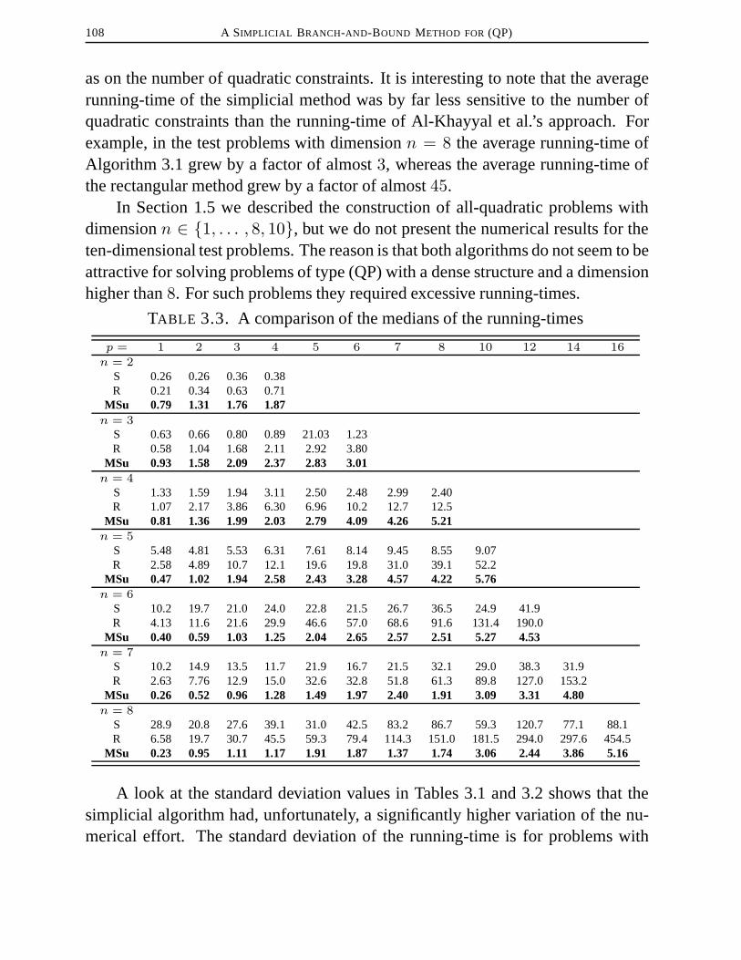
108 A SIMPLICIAL BRANCH-AND-BOUND METHOD FOR(QP)
as on the number of quadratic constraints. It is interesting to note that the averagerunning-time of the simplicial method was by far less sensitive to the number ofquadratic constraints than the running-time of Al-Khayyal et al.’s approach. Forexample, in the test problems with dimensionn = 8 the average running-time ofAlgorithm 3.1 grew by a factor of almost3, whereas the average running-time ofthe rectangular method grew by a factor of almost45.
In Section 1.5 we described the construction of all-quadratic problems withdimensionn ∈ {1, . . . , 8, 10}, but we do not present the numerical results for theten-dimensional test problems. The reason is that both algorithms do not seem to beattractive for solving problems of type (QP) with a dense structure and a dimensionhigher than8. For such problems they required excessive running-times.
TABLE 3.3. A comparison of the medians of the running-times
p = 1 2 3 4 5 6 7 8 10 12 14 16
n = 2S 0.26 0.26 0.36 0.38R 0.21 0.34 0.63 0.71
MSu 0.79 1.31 1.76 1.87n = 3
S 0.63 0.66 0.80 0.89 21.03 1.23R 0.58 1.04 1.68 2.11 2.92 3.80
MSu 0.93 1.58 2.09 2.37 2.83 3.01n = 4
S 1.33 1.59 1.94 3.11 2.50 2.48 2.99 2.40R 1.07 2.17 3.86 6.30 6.96 10.2 12.7 12.5
MSu 0.81 1.36 1.99 2.03 2.79 4.09 4.26 5.21n = 5
S 5.48 4.81 5.53 6.31 7.61 8.14 9.45 8.55 9.07R 2.58 4.89 10.7 12.1 19.6 19.8 31.0 39.1 52.2
MSu 0.47 1.02 1.94 2.58 2.43 3.28 4.57 4.22 5.76n = 6
S 10.2 19.7 21.0 24.0 22.8 21.5 26.7 36.5 24.9 41.9R 4.13 11.6 21.6 29.9 46.6 57.0 68.6 91.6 131.4 190.0
MSu 0.40 0.59 1.03 1.25 2.04 2.65 2.57 2.51 5.27 4.53n = 7
S 10.2 14.9 13.5 11.7 21.9 16.7 21.5 32.1 29.0 38.3 31.9R 2.63 7.76 12.9 15.0 32.6 32.8 51.8 61.3 89.8 127.0 153.2
MSu 0.26 0.52 0.96 1.28 1.49 1.97 2.40 1.91 3.09 3.31 4.80n = 8
S 28.9 20.8 27.6 39.1 31.0 42.5 83.2 86.7 59.3 120.7 77.1 88.1R 6.58 19.7 30.7 45.5 59.3 79.4 114.3 151.0 181.5 294.0 297.6 454.5
MSu 0.23 0.95 1.11 1.17 1.91 1.87 1.37 1.74 3.06 2.44 3.86 5.16
A look at the standard deviation values in Tables 3.1 and 3.2 shows that thesimplicial algorithm had, unfortunately, a significantly higher variation of the nu-merical effort. The standard deviation of the running-time is for problems with

3.5. COMPUTATIONAL RESULTS 109
n ≥ 5 almost always higher than the corresponding average value (see Table 3.2).We even have combinations ofn andp, where the standard deviation is more than3 times larger than the average value. The rectangular algorithm did not have thisproperty. The standard deviation of running-times is mostly smaller than the aver-age value. This shows that the rectangular algorithm had a more robust behaviorthan the simplicial one in the sense that the effort for solving problems with thesame dimension and the same number of quadratic constraints did not vary so keen.In spite of that higher variation of the effort for solving all-quadratic problems, Al-gorithm 3.1 was almost always faster and led on average to a substantial speedup,at least for problems with higher number of quadratic constraints. If we neglect thenumerical outliers leading to the high standard deviation values, then there holdsthat Algorithm 3.1 showed an even better relative performance. In Table 3.3 themedians of the running-times for all tested combinations (n, p) together with themedian speedup coefficients (MSu) are displayed, where this speedup coefficient isagain the quotient of the median of the running-time for the rectangular algorithm(R) and the corresponding value for Algorithm 3.1 (S). This table shows that, withrespect to the medians, Algorithm 3.1 was also for higher dimensional problemsandp = 2n about5 times faster than Al-Khayyal et al.’s rectangular approach(compare with the speedup coefficients in Table 3.2).
3.5.3. A Modification of Algorithm 3.1. We finish the numerical examina-tion of Algorithm 3.1 by considering a slight modification of this approach. InRemark 3.2.2(b) we pointed out that the LP-relaxation (LPS) of (QPS) depends onthe numbering of the vertices ofS = [v0, . . . , vn], in particular on the choice ofv0. In the numerical tests we described till now, we did not care about the choiceof this vertex. Since we did not apply any rule, it was somehow randomly whichvertex of the considered simplexSkj (k ∈ IN; j = 1, 2) was the first one.
In the sequel we will see that a special choice of this vertex can lead to numer-ical improvements of our approach. There are of course many possible decisionrules for choosingvk0 , which could depend on the function values ofq0 at the ver-tices, or on the function values of then + 1 possible affine underestimating func-tions, or also on the behavior of the quadratic constraintsql (l ∈ {1, . . . , p}) andon the behavior of their underestimators. We tested several rules and would like topresent only the one, which showed the best performance in our numerical tests.
Let S = [v0, . . . , vn] be an arbitraryn-simplex and let, forj ∈ {0, . . . , n},`0,jS : IRn → IR be the affine underestimating function forq0 onS constructed with

110 A SIMPLICIAL BRANCH-AND-BOUND METHOD FOR(QP)
respect to the vertexvj , i.e.,
`0,jS (x) =n∑
i=0,i6=j
((W j
S)−1(x− vj))i(vi − vj)TD0(vi − vj)
+(d0 + 2Q0vj
)T(x − vj) + (d0)T vj + vTj Q
0vj ,
where W jS denotes the realn × n matrix with the columns(vi − vj)
(i ∈ {0, . . . , n} \ {j}). Consider the maximal distance of the objective functionq0 and the function0,j
S (j ∈ {0, . . . , n}) at the vertices ofS. It can be verified bystraightforward calculation that there holds
maxi=0,... ,n
[q0(vi)− `0,jS (vi)
]= max
i=0,... ,n(vi − vj)TC0(vi − vj) .
Among thesen + 1 possibilities for the function0S we choose one, where the
minimum of these maximal distances is attained, i.e., we choosej0 ∈ {0, . . . , n}satisfying
maxi=0,... ,n
(vi − vj0)TC0(vi − vj0) = minj=0,... ,n
[max
i=0,... ,n(vi − vj)TC0(vi − vj)
].
In Algorithm 3.1 this means that we interpretvj0 as the first vertex ofS, i.e.,S = [vj0 , v0, . . . , vj0−1, vj0+1, . . . , vn], and construct the affine functions`lS(l ∈ {0, . . . , p}) with respect to this vertex.
This decision rule for the choice of the first vertex ofSkj (k ∈ IN, j = 1, 2) ledto an improvement of the numerical performance of our approach. By applying thisrule we could reduce the effort for solving our test problems. In Table 3.4 the pro-portional reductions of the average number of linear subproblems are displayed for
TABLE 3.4. Proportional reduction of the average number ofLP’s by applying a special selection rule for the first vertexvk0
n p 1 2 3 4 5 6 7 8 10 12 14 16
2 9.92 9.96 5.30 6.673 13.1 18.1 14.8 10.9 14.7 15.04 16.0 21.7 19.3 21.9 16.5 32.5 16.8 15.35 17.4 21.6 30.2 27.1 28.1 16.5 22.3 23.3 16.86 23.4 25.7 33.5 34.9 25.4 34.4 25.4 31.4 24.0 26.17 2.22 37.8 36.2 37.6 37.2 34.4 34.6 32.2 29.4 31.6 31.28 55.6 28.1 46.5 24.1 45.6 32.4 35.2 34.4 43.9 42.3 41.1 39.9

3.5. COMPUTATIONAL RESULTS 111
all combinations of the dimensionn and the number of quadratic constraintsp ex-amined in our numerical tests. This proportional reduction is calculated accordingto
AvgNuLP(A)− AvgNuLP(B)AvgNuLP(A)
· 100% .
AvgNuLP(A) denotes the average number of linear subproblems needed by Algo-rithm 3.1 without any rule for the choice of the first vertex. AvgNuLP(B) is thecorresponding value, when the above decision rule was applied. This table showsthat the application of the proposed selection rule was able to reduce the averagenumber of LP’s by up to50%. Since this selection rule is not time-consuming –from a computational point of view – we obtained almost the same reduction in theaverage running-times of Algorithm 3.1.
It is interesting to note that the numerical improvement increased with grow-ing dimension. A reason for this effect might be that with growing dimension thenumber of possibilities for choosing the first vertex increases. For small dimen-sional problems we have a high probability that the choice ofvk0 according to ourspecial rule and the random choice ofvk0 coincide. Hence, we obtain only a slightdifference in the numerical effort. However, for higher dimensional problems thisprobability decreases and the positive results in Table 3.4 corroborate that our se-lection rule for the first vertex was a good choice in the sense that the lower bounds,which we obtained by applying this rule, were mostly better than the one obtainedwithout using any rule. Another remarkable result of Table 3.4 is that the numericalimprovement did not depend on the number of quadratic constraints. Nevertheless,it can be possible that an additional consideration of the quadratic constraints in theselection rule for the first vertex leads to a further improvement of Algorithm 3.1.
The simplicial branch-and-bound method presented in this chapter used bi-section as a subdivision rule for simplices. In Remark 3.4.1(a) we pointed outthat Property (3.4.1) of this rule is substantial for the convergence of our approach.Some authors favor another subdivision rule. In this so-calledω-subdivisionrule ann-simplexSk is subdivided into up ton+ 1 subsimplices by using a radial subdi-vision with respect to the optimal solutionω(Sk) of the current LP-relaxation onSk (see Definition 1.2.2). One hopes that this point bears some information of theoriginal problem (QP), and hence one expects that this rule leads to better numer-ical results. However, this subdivision rule has not Property (3.4.1) such that theconvergence of a simplicial branch-and-bound method, which is based on this rule,

112 A SIMPLICIAL BRANCH-AND-BOUND METHOD FOR(QP)
is still an open question. In the next chapter we will give an answer to this theo-retical problem. We will consider a generalization of Algorithm 3.1, which usesconvex subproblems and is able to deal with a more general problem class.
CHAPTER 4
On the Convergence of Simplicial Branch-and-BoundMethods
In this chapter we are interested in a generalization of the all-quadratic optimizationproblem studied in this thesis. We treat problems of the form
min g0(x) + f0(x)
gl(x)+f l(x) ≤ 0 l = 1, . . . , p
x ∈ P ,
(DCP)
wheregl : IRn → IR (l = 0, . . . , p) are convex functions,f l : IRn → IR(l = 0, . . . , p) are concave functions, andP = {x ∈ IRn : Ax ≤ b} withA = (a1, . . . , am)T ∈ IRm×n, b ∈ IRm is a non-empty and full-dimensionalpolytope. Problems of this form belong to the class ofgeneral d.c. problemssincethe objective function and a part of the constraint functions can be written as adifference of twoconvex functions (see, e.g., [HPT95, TUY95, HT96B] for theframework of d.c. problems). We denote by
F := {x ∈ IRn : Ax ≤ b , gl(x) + f l(x) ≤ 0 , l = 1, . . . , p}the feasible region of Problem (DCP).
4.1. Introduction
In the following we distinguish three subclasses of (DCP):
(DCP1) g0 ≡ 0, p = 0, i.e., minimization of a concave function over a polytope;(DCP2) gl ≡ 0 (l = 1, . . . , p), i.e., minimization of a d.c. function over a feasible
region described by a polytope and by reverse convex constraints;(DCP3) ∃l ∈ {1, . . . , p}: gl 6= 0, i.e., minimization of a d.c. function over a non-
polyhedral set.
113

114 ON THE CONVERGENCE OFSIMPLICIAL BRANCH-AND-BOUND METHODS
It is well-known that the optimal valuef? of a problem of type (DCP1) isattained in at least one vertex ofP [HPT95, Theorem 1.19]. Nevertheless, thisproblem class was proven to be NP-hard. NP-hardness holds even in very specialcases, such as problems whose objective function is concave quadratic and whosefeasible region is a hypercube (see, e.g., [PS88]).
This class of global optimization problems encompasses a wide variety of ap-plications. Among them we recall problems witheconomies of scale, where con-cave costs arise because of decreasing marginal costs, andminimum concave costflow problems, i.e., flow problems in which the cost functions of the arcs are con-cave. Moreover, some well-known mathematical problems can be reformulatedas concave optimization problems, for instanceinteger programming[PS76] andlinear complementarity problems(see, for example, [HPT95, pages 69-70]).
Different approaches to the solution of (DCP1) were proposed in the litera-ture. They can be subdivided in three classes: enumerative methods, successiveapproximation methods and branch-and-bound methods. The first two classes ofalgorithms are mostly guaranteed to return an optimal solution in finite time by ex-ploring, in the worst case, all the vertices ofP . Branch-and-bound methods cangenerally only be guaranteed to be convergent. On the other hand, algorithms fromthis class are often efficient in practice.
The class of branch-and-bound methods can be further subdivided in threesubclasses according to the kind of partition sets they employ (see also Subsec-tions 1.2.2 and 1.2.3):conical algorithms, first introduced in [TUY64], rectan-gular algorithms, first introduced in [FS69], andsimplicial algorithms, first in-troduced in [HOR76]. For further, more detailed information about theory, al-gorithms and applications in the field of concave optimization over a polytopewe refer to the quite extensive literature on the subject, including, in particular,[HOR84, PR86, BEN95, HPT95, HT96B].
If the objective function of a problem of type (DCP2) is linear and there is onlyone concave constraint, i.e.,p = 1, then this problem is acanonical d.c. problem
min cTxf(x) ≥ 0x ∈ P ⊂ IRn
(DCP2)
with f(x) := −f1(x) (see, e.g., [HPT95] or [TUY95] for the definition of thecanonical d.c. problem). It is known that, under mild regularity conditions, theoptimal valuef? of (DCP2) is attained at a pointx? on an edge ofP satisfyingf(x?) = 0 [HPT95, Theorem 4.4] .

4.1. INTRODUCTION 115
The class (DCP2) of global optimization problems is not so widely exploredin the literature. The articles on d.c. programming consider mostly the canonicald.c. problem or a general d.c. problem of the form (DCP3). Our differentiationbetween (DCP2) and (DCP3) is theoretically motivated, as we will see in the nextsections. An application of problem class (DCP2) is the packing problem(seeSection 1.3 and particularly Chapter 5 for details). Problems with a d.c. objec-tive function, linear constraints and Boolean variables can also be transformed toproblems of type (DCP2) (xi ∈ {0, 1} ⇔ x2
i − xi ≥ 0, xi ∈ [0, 1]).Using the fact that an optimal solution of the canonical d.c. problem is attained
on an edge of the polytopeP a special finite solution method for this problemclass was developed in [TT85] (modified in [HPT95]). If the objective function of(DCP2) is nonlinear or if there is more than one concave constraint then, extendingthe ideas used for solving problems of type (DCP1), Problem (DCP2) can be solvedby branch-and-bound methods, as we will see in subsequent sections.
The class of d.c. functions defined on a compact convex set ofIRn is dense inthe set of continuous functions [HPT95, Corollary 4.2]. Furthermore, the set ofd.c. functions is closed with respect to arbitrary linear combinations, finite maxi-mizations, finite minimizations and multiplications [HPT95, Theorem 4.1]. There-fore, the class of general d.c. problems encompasses a wide variety of problemclasses and applications. However, finding a representation of a d.c. function as adifference of two convex functions, which we assume to be given in the formula-tion of problem type (DCP3), is in general a hard, still open problem. For the all-quadratic problems such a representation is easy to generate as we saw in Chapter3. They are also known for many interesting function classes. Among the variousapplications of d.c. problems of type (DCP3) we recall thebridge location problem(see [HT99]), thegeneral location problem(see, for example, [ILM88]) and thedesign centering problem[VS82, THA88, NS92]. Similar to problems of type(DCP2) general d.c. problems of type (DCP3) can be solved by branch-and-boundmethods. In order to avoid convex subproblems in such approaches, the branch-and-bound methods are often combined with an outer approximation scheme (see[HT99] and, in particular, [TUY95] and references therein).
In this chapter simplicial branch-and-bound methods for solving all types of(DCP) are considered. In particular, simplicial algorithms based on the so-calledω-subdivision, a special subdivision rule, first introduced in [TUY64] for conicalbranch-and-bound algorithms and applied for simplicial approaches, for example,in [HT96B], are studied. As long as a so-calledexhaustivesubdivision rule is used,

116 ON THE CONVERGENCE OFSIMPLICIAL BRANCH-AND-BOUND METHODS
the convergence of the simplicial branch-and-bound method suggested in the nextsection can be ensured. The convergence of this algorithm usingω-subdivision,which is not necessarily exhaustive, was an open theoretical question for a longtime. Recently, a similar question was answered for conical branch-and-bound al-gorithms used for solving (DCP1) independently and by different techniques in[JM98] and [LOC97]. However, to the author’s knowledge, no proof of conver-gence for simplicial algorithms, which base only onω-subdivisions, has been pub-lished yet.
In the next section the general scheme of the studied simplicial branch-and-bound algorithm is given, and in Section 4.3 the convergence of this approach basedon an exhaustive subdivision rule is proved. This convergence result corresponds tothe one obtained in the previous chapter for Algorithm 3.1 (see Theorem 3.4.2). Ifwe useω-subdivision, then a similar convergence result for the proposed algorithm,used for solving problems of type (DCP1), can also be proven. In order to show,additionally, a convergence result for this approach, applied for problems of type(DCP2), we need an assumption with respect to the concave partf0 of the objectivefunction. This assumption is not a restriction, as we will see in Section 4.4. Thoughthe obtained convergence result for this case will be theoretically weaker than theone before, – from a practical point of view – all convergence results derived inthis chapter have the same quality. They imply that the proposed approach detectsin finite time either the emptiness ofF or an approximate solution of the consid-ered problem. The proofs of the statements yielding these convergence results forour approach usingω-subdivisions are given together in Section 4.4 for both sub-classes of (DCP). Even though the convergence results are slightly different, theirderivation is non the less connected. The part of the proofs relating to Problem(DCP1) is equivalent to the convergence proofs in [LR97B]. In Section 4.5 we pro-pose an example, which shows that the simplicial branch-and-bound method usingω-subdivisions for solving problems of type (DCP3) is not necessarily convergent.We conclude the consideration of the convergence in Section 4.6 with a numericalcomparison of the simplicial branch-and-bound algorithm with different subdivi-sion rules for solving all-quadratic optimization problems of type (DCP3). In par-ticular, we suggest in this section a modification of theω-subdivision, which leadsto a convergent algorithm also for problems of the general class (DCP3). In the lastSection 4.7 a partial answer to the theoretical problem of finiteness of the simplicialbranch-and-bound algorithm withω-subdivision, applied for solving problems oftype (DCP1), is presented. This finiteness result is also given in [LR97A].

4.2. SIMPLICIAL ALGORITHMS FOR(DCP) 117
4.2. Simplicial Algorithms for (DCP)
In this section we describe a simplicial branch-and-bound algorithm for solv-ing Problem (DCP). The formulation is a generalization of the one given in Chapter3 (see Algorithm 3.1). Before giving the exact description we recall some notations,which will be extensively used in the following.
• Let, for r ∈ IN, r ≤ n,
Br := {λ ∈ IRr+1 :r∑i=0
λi = 1 , λi ≥ 0 , i = 0, . . . , r }
be the standardr-simplex inIRr+1.• Let S = [v0, . . . , vn] be ann-simplex andl ∈ {0, . . . , p}. The affine
functionϕlS : IRn → IR,
ϕlS(x) =n∑i=0
λ(x)if l(vi) (4.2.1)
is the convex envelope off l over S (see, e.g., [HPT95] or Subsection1.2.4). The vectorλ(x) ∈ {λ ∈ IRn+1 :
∑ni=0 λi = 1} denotes the
uniquely determined barycentric coordinates ofx ∈ IRn with respect to thevertex set{v0, . . . , vn} of S, i.e.,x =
∑ni=0 λ(x)ivi. Let ζlS ∈ IRn be the
unique solution of the following system of equations
(ζlS)T (vi − v0) = f l(vi)− f l(v0) i = 1, . . . , n .
Then there holds, forx ∈ IRn,
ϕlS(x) = (ζlS)T (x− v0) + f l(v0) . (4.2.2)
• Let S = [v0, . . . , vn] be ann-simplex. For eachj ∈ {0, . . . , n}, choosei(j) ∈ {0, . . . , n} \ {j} and letvSj ∈ IRn be the unique solution of thesystem of linear equations
(vSj )T (vi − vi(j)) = 0 i ∈ {0, . . . , n} \ {j, i(j)} (4.2.3.a)
(vSj )T (vj − vi(j)) = −1 . (4.2.3.b)
Then, withcSj := (vSj )T vi(j), then-simplexS can be represented by thesystem of linear inequalities
(vSj )Tx ≤ cSj j = 0, . . . , n . (4.2.4)

118 ON THE CONVERGENCE OFSIMPLICIAL BRANCH-AND-BOUND METHODS
The vector vSj is the normal of the facet[v0, . . . , vj−1, vj+1, . . . , vn]of S.
In Chapter 3 (see, in particular, Section 3.4) we pointed out that it is neces-sary to be satisfied with approximate solutions of all-quadratic problems of type(QP), if we are interested in a finite solution approach. The finiteness of the sim-plicial branch-and-bound method for Problem (DCP) to be discussed in the presentchapter, can also only be obtained, if approximate feasible respectively optimal so-lutions are sufficient. Therefore, we introduce the concept of(δ,ρ)-feasiblepointsand of(ε,δ,ρ)-solutionsof Problem (DCP).
DEFINITION 4.2.1. A point x ∈ IRn is called (δ,ρ)-feasible for Problem(DCP) with real numbersδ, ρ ≥ 0, if there holds
aTj x− bj ≤ ρ j = 1, . . . ,m (4.2.5.a)and
gl(x) + f l(x) ≤ δ l = 1, . . . , p . (4.2.5.b)
A pointx ∈ IRn is called an(ε,δ,ρ)-solution for Problem (DCP) with real numbersε,δ,ρ ≥ 0, if there holds
x is (δ,ρ)-feasible (4.2.6.a)and
g0(x) + f0(x)− ε ≤ minx∈F
[g0(x) + f0(x)
], (4.2.6.b)
where the right-hand side of (4.2.6.b) is defined as∞, if F is empty.
For ρ = 0 we say thatx is a δ-feasible point, forδ = ρ = 0 x is a feasiblepoint and forε = δ = ρ = 0 x is an optimal solution of (DCP). Note that for an(ε,δ,ρ)-solutionx ∈ IRn it is not necessary that there holds
g0(x?) + f0(x?) ≤ g0(x) + f0(x) ,
wherex? denotes the optimal solution of (DCP), ifF 6= ∅. Therefore, Condition(4.2.6.b) does not guarantee that the objective function value ofx has a distancesmaller thanε to the optimal one (see, in particular, the caseF = ∅). This distancedepends on the choice ofδ andρ and on the behavior of the objective function of(DCP) on the set
Fδ,ρ := {x ∈ IRn : aTj x− bj ≤ ρ , j = 1, . . . ,m,gl(x) + f l(x) ≤ δ , l = 1, . . . , p} .
If, however,x is feasible, thenx is ε-optimal in the sense of
|g0(x) + f0(x)− g0(x?)− f0(x?)| ≤ ε .

4.2. SIMPLICIAL ALGORITHMS FOR(DCP) 119
In order to formulate the simplicial branch-and-bound method for Problem(DCP) we need a convex relaxation of (DCP) with respect to a given simplex. LetS = [v0, . . . , vn] be ann-simplex. The set
FS := {x ∈ S : Ax ≤ b , gl(x) + ϕlS(x) ≤ 0 , l = 1, . . . , p} (4.2.7)
is convex withFS ⊃ F ∩ S. If FS is non-empty, we know that the optimalsolutionµ?(S) of the convex optimization problem
min g0(x) + ϕ0S(x)
x ∈ FS(DCPS)
is a lower bound for minx∈F∩S
[g0(x) + f0(x)
], i.e., (DCPS) is a convex relaxation
of (DCP). In the following we denote by (DCPSi ) (i = 1, 2, 3) the proposed convexrelaxation of Problem (DCPi) (i = 1, 2, 3) with respect to the simplexS. Note that(DCPS1 ) is a linear optimization problem, (DCPS2 ) is a convex optimization prob-lem with linear constraints and (DCPS3 ) is an optimization problem with a convexobjective function as well as convex constraints.
In general, it is not possible to solve exactly the convex optimization problem(DCPS) in finite time. We are only able to assume that a solution method for(DCPS) is known, which solves the problem in finite time with arbitrary accuraciesε, δ, ρ > 0. This means, if such a method does not detect the emptiness ofFS , itgenerates a pointx with the properties
aTj x− bj ≤ ρ j = 1, . . . ,m , (4.2.8.a)
(vSi )T x− cSi ≤ ρ i = 0, . . . , n , (4.2.8.b)
gl(x) + ϕlS(x) ≤ δ l = 1, . . . , p (4.2.8.c)and
g0(x) + ϕ0S(x)− ε ≤ min
x∈FS
[g0(x) + ϕ0
S(x)]
= µ?(S) . (4.2.8.d)
According to Definition 4.2.1,x is an (ε, δ, ρ)-solution of Problem (DCPS). Notethat it is possible that the used method stops with a (δ, ρ)-feasible point, eventhough the feasible regionFS is empty. In each case
µ(S) := g0(x) + ϕ0S(x)− ε (4.2.9)
is a lower bound forµ?(S), sinceµ?(S) is defined as∞ in the empty case. In thefollowing we denote byCONVEXSOLVERε,δ,ρ (ε, δ, ρ ≥ 0) a solution method forProblem (DCPS), which detects after finite time either the emptiness ofFS or apoint x with Properties (4.2.8.a)-(4.2.8.d).

120 ON THE CONVERGENCE OFSIMPLICIAL BRANCH-AND-BOUND METHODS
REMARK 4.2.1.
(a) Since (DCPS1 ) is a linear optimization problem we can use the Simplex-Algorithm as aCONVEXSOLVER0,0,0.
(b) If the objective function of (DCPS2 ) is quadratic with a positive definiteHessian, then several solution methods exist. For example, this problem isequivalent to a linear complementarity problem (LCP) and, therefore, thereexists also aCONVEXSOLVER0,0,0. For an overview on the relation be-tween convex quadratic optimization problems and LCP‘s and for solutionmethods for LCP‘s we refer to [CPS92].
(c) In Section B.1 aCONVEXSOLVERε,δ,0 , which bases on the KCG-cutting-plane-method [CG59, KEL60] and needs no additional assumptions on theinvolved nonlinear functions beside of their convexity, is presented. Forextensions of this method we refer to [HTT87, HT96B] and referencestherein.
(d) If an (ε, δ, 0)-solution of Problem (DCPS) is required, it is possible to ad-just an arbitraryCONVEXSOLVERε,δ,ρ in such a way that the calculatedpoint x ∈ IRn is feasible with respect to the linear constraints. If aCON-VEXSOLVERε,δ,ρ delivers a pointx /∈ P ∩ S and the accuracies are chosensufficiently small, then we can use the orthogonal projection pointx of xon the polytopeP ∩ S as an (ε, δ, 0)-solution of Problem (DCPS). Howthis can be done and, in particular, how the accuraciesε, δ andρ have to bechosen, is described in Section B.2.
For the formulation of the algorithm we assume further that a real numberη <∞ with the property
η ≥
minx∈F
[g0(x) + f0(x)
], if F 6= ∅
maxx∈P
[g0(x) + f0(x)
], otherwise
, (4.2.10)
is known. If a feasible pointx ∈ F is known in advance, then we can useη := g0(x) + f0(x). Otherwise by setting
η := maxx∈P
[ψ0S(x) + f0(x)
], (4.2.11)
whereψ0S : IRn → IR denotes the concave envelope ofg0 with respect to an arbi-
traryn-simplexS ⊃ P , we get the required value. Note that (4.2.11) is a concavemaximization problem, which can be solved by an arbitraryCONVEXSOLVERε,δ,ρ.

4.2. SIMPLICIAL ALGORITHMS FOR(DCP) 121
If the accuracyε is greater than0, we have to adjust the calculatedoptimal valueof (4.2.11) withε in order to obtain a real number with Property (4.2.10).
The description of the algorithm follows the guidelines of a basic branch-and-bound algorithm given in [HPT95, Algorithm 3.5] and is similar to Algorithm 3.1discussed in Chapter 3.
ALGORITHM 4.1 (Simplicial Branch-and-Bound Algorithm for (DCP) ).
InitializationChoose real numbersε, δ, ρ ≥ 0 and sequences{εk}k∈IN0 , {δk}k∈IN0 ,
{ρk}k∈IN0 with εk, δk, ρk ≥ 0 (k ∈ IN0) andεk, δk, ρk → 0 (k →∞).
Determine ann-simplexS0 = [v00 , . . . , v
0n] with S0 ⊃ P .
Q← {v0i : i = 0, . . . , n with v0
i is (δ,ρ)-feasible}If CONVEXSOLVERε0,δ0,ρ0 detectsFS0 = ∅ Then
STOP← True (F = ∅)Else
Let ω(S0) be an (ε0, δ0, ρ0)-solution of (DCPS0) and
µ(S0) = g0(ω(S0)) + ϕ0S0(ω(S0)) be the corresponding function value.
µ(S0)← µ(S0)− ε0, µ0 ← µ(S0) , P ← {S0}If ω(S0) is (δ, ρ)-feasibleThen Q← Q ∪ {ω(S0)}If Q 6= ∅ Thenη0 ← min
x∈Q[g0(x) + f0(x)
]Choosexf ∈ Q with η0 = g0(xf ) + f0(xf ) .
Elseη0 ← η + ε+ τ (τ > 0 arbitrary)
EndIfSTOP← False, k ← 0
EndIf
While STOP= False DoIf ηk − µk ≤ ε Then (SC)
STOP← True (xf is an (ε, δ, ρ)-solution of (DCP) )Else
Choosewk ∈ Sk\{vk0 , . . . , vkn} and set (PSR)Ik ← {i ∈ {0, . . . , n} : λki > 0 with λk ∈ Bn ,
∑nj=0 λ
kj vkj = wk }

122 ON THE CONVERGENCE OFSIMPLICIAL BRANCH-AND-BOUND METHODS
If wk is (δ, ρ)-feasibleThen Q← Q ∪ {wk}For j ∈ Ik DoSkj ← [vk0 , . . . , v
kj−1, w
k, vkj+1, . . . , vkn] ⊂ Sk
If CONVEXSOLVERεk,δk,ρk does not detectFSkj
= ∅ Then
Letω(Skj ) be an (εk, δk, ρk)-solution of (DCPSkj ) andµ(Skj ) =
g0(ω(Skj )) + ϕ0Sk
j
(ω(Skj )) be the corresponding function value.
µ(Skj ) ← max{µ(Skj )− εk, µk} (LBR)
If ω(Skj ) is (δ, ρ)-feasibleThen Q← Q ∪ {ω(Skj )}P ← P ∪ {Skj }
EndIfEndForP ← P\{Sk}If Q 6= ∅ Thenηk+1 ← min
x∈Q[g0(x) + f0(x)
]Choosexf ∈ Q with ηk+1 = g0(xf ) + f0(xf ) .
Elseηk+1 ← ηk
EndIfP ← P\{S ∈ P : µ(S) ≥ ηk+1 − ε} (PR)
If P 6= ∅ Thenµk+1 ← min
S∈Pµ(S)
ChooseSk+1 ∈ P with µk+1 = µ(Sk+1). (SSR)Else
If Q 6= ∅ Thenµk+1 ← ηk+1 − ε
ElseSTOP← True (F = ∅)
EndIfEndIfk ← k + 1
EndIfEndWhile

4.2. SIMPLICIAL ALGORITHMS FOR(DCP) 123
REMARK 4.2.2.
(a) P is assumed to be a non-empty full-dimensional polytope. Therefore,there exists always ann-simplexS0 with S0 ⊃ P . For the constructionpossibilities we refer to [HPT95, pp. 145f].
(b) Since we are in general – as mentioned before – not able to solve the convexsubproblems exactly, we cannot guarantee that there holds
µ(Skj ) ≥ µ(Sk) = µk ,
even though we know thatSkj ⊂ Sk. In order to generate a non-decreasingsequence of lower bounds we use the lower bounding rule (LBR).
(c) The deletion of the simplices in the classicalpruning rule(PR) is the conse-quence of the fact thatµ(S) is a lower bound ofminx∈F∩S
[g0(x) + f0(x)
](see (4.2.9)). IfP is empty after executing this rule andQ is not empty, thenit is obvious thatηk+1 − ε is a lower bound for the optimal value of (DCP).
(d) Each (δ, ρ)-feasible point for (DCP) generated during the solution of theconvex subproblems should be affiliated to the setQ in order to possiblyimprove the upper boundηk.
(e) The algorithm has to generate at least one (δ, ρ)-feasible point for Problem(DCP), such that the stopping criterion (SC) can be satisfied. If no feasiblepoint is known in advance, it follows immediately from Property (4.2.10) ofη that, for each simplexS generated during the execution of the algorithm,there holds
µ(S) ≤ η = η0 − ε− τ .
Therefore, without an update ofηk+1 different fromηk the stopping cri-terion (SC) cannot be fulfilled. Moreover, taking the pruning rule into ac-count, we know that (SC) can only be satisfied in iterationk ≥ 2, if thereholdsP = ∅ andQ 6= ∅ at the end of the previous iteration (compare withRemark 3.3.1(d)).
(f) It is possible that Algorithm 4.1 generates an (ε, δ, ρ)-solution of Problem(DCP) withε, δ, ρ > 0, even ifF = ∅.
(g) Since we choosewk /∈ {vk0 , . . . , vkn} in the point selection rule (PSR) it isensured that there holdsIk 6= ∅. Note that the used subdivision ofSk is aradial subdivision (see Definition 1.2.2), which forms a partition ofSk (seeDefinition 1.2.1 and [HPT95, Proposition 3.7]).

124 ON THE CONVERGENCE OFSIMPLICIAL BRANCH-AND-BOUND METHODS
(h) If there holds, for an iterationk ∈ IN, ε ≥ εk, δ ≥ δk andρ ≥ ρk and,additionally, if ω(Skj ) is a vertex of the simplexSkj (j ∈ Ik), then weknow that this simplexSkj is fathomed in the pruning rule (PR). Indeed, letω(Skj ) be a vertex ofSkj . It follows that the function value of each concavefunction f l (l ∈ {0, . . . , p}) at the pointω(Skj ) coincides with the func-tion value of the corresponding convex envelopeϕl
Skj
. The pointω(Skj )
is at least (δ, ρ)-feasible for Problem (DCPSkj ) and, consequently, also
(δ, ρ)-feasible for Problem (DCP), i.e.,ω(Skj ) is used for updating the upperboundηk+1. It follows that
µ(Skj ) ≥ g0(ω(Skj )) + ϕ0Sk
j(ω(Skj ))︸ ︷︷ ︸
=f0(ω(Skj))
−ε ≥ ηk+1 − ε ,
i.e.,Skj must be fathomed in the pruning rule (PR).
The construction ofµk (k ∈ IN) guarantees that this value is always a lowerbound forg0(x) + f0(x) with respect to the whole feasible regionF . Therefore, itis obvious that, when finite, the algorithm will determine either an (ε, δ, ρ)-solution(ε, δ, ρ ≥ 0) of (DCP) or the emptiness ofF . How far it is possible to provethe finiteness of Algorithm 4.1 withε, δ, ρ > 0, respectively the convergence forε = δ = ρ = 0, depends on the choice of the rule to split the current simplexSk.The subdivision rule applied in Algorithm 4.1, which is determined by the selectionof the pointwk (see the point selection rule (PSR) in the formulation of Algorithm4.1), is also a critical one with respect to the efficiency of the presented approach(see, e.g., [TUY91A] or the numerical results in Section 4.6).
There exist two classical subdivision rules. In the so-calledbisection, whichwas first introduced in [HOR76] for simplicial algorithms,wk is chosen as themidpoint of the longest edge of the current simplexSk = [vk0 , . . . , v
kn]. Let
i0, i1 ∈ {0, . . . , n} be two indices corresponding to vertices ofSk with the longestEuclidean distance, i.e.,
‖vki0 − vki1‖2 = maxi,j=0,... ,n
‖vki − vkj ‖2 . (4.2.12)
Then we choose
wk :=vki0 + vki1
2.

4.2. SIMPLICIAL ALGORITHMS FOR(DCP) 125
This is the subdivision rule, we chose in the formulation of Algorithm 3.1 (seeSection 3.3).
If we apply the so-calledω-subdivision (see, e.g., [TUY64, HT96B]), thenwe subdivide the current simplexSk with respect to the calculated solutionω(Sk)of the subproblem (DCPS
k
). In the classicalω-subdivision rule, as it is described,e.g., in [HT96B], the pointwk is chosen asω(Sk). Since it is assumed there thatω(Sk) is feasible with respect to the relevant simplexSk and, additionally, feasiblewith respect to the original problem, i.e.,ω(Sk) ∈ F ∩ Sk, it is clear (see Remark4.2.2(h)) that in this situation there holdsω(Sk) ∈ Sk \ {vk0 , . . . , vkn}.
In the formulation of Algorithm 4.1 we use aCONVEXSOLVERεk,δk,ρk withεk, δk, ρk ≥ 0 (k ∈ IN). Therefore, in general we cannot expect thatω(Sk) iscontained inSk, and, in particular, we do not know anything about the feasibilityof ω(Sk) with respect to the original Problem (DCP). For that reason, we cannotchoosewk = ω(Sk) in each case and we need, thus, a generalization of the classicalω-subdivision rule. A possible choice ofwk is the following, which we would liketo call thegeneralizedω-subdivision rule (GWSR):
Chooseλk ∈ {λ ∈ IRn+1 :∑n
i=0 λi = 1} with ω(Sk) =∑ni=0 λ
ki vki .
Ik ← {i ∈ {0, . . . , n} : λki > 0}If |Ik| = 1 Thenwk ← 1
2
(vki0 + vki1
)(i.e., choose a bisection)
ElseDetermineγk :=
∑i∈Ik λki
For i = 0 To n DoIf i ∈ Ik Then
λki ← λki
γk
Elseλki ← 0
EndIfEndForwk ← ∑n
i=0 λki vki
EndIf

126 ON THE CONVERGENCE OFSIMPLICIAL BRANCH-AND-BOUND METHODS
Theω-subdivision rule, which is connected to the information returned by thealgorithm inside the selected simplex, seems to be the more natural choice thanbisection, at least for problems of type (DCP1). On the other hand, while Algo-rithm 4.1 based on bisections can be proven to be convergent (see Section 4.3), thesame is in general not true for the variant of Algorithm 4.1, which employs onlyω-subdivisions, as the counterexample in Section 4.5 shows.
If we solve problems of type (DCP1), we can chooseεk = δk = ρk = 0(k ∈ IN0) in the initialization of Algorithm 4.1 since (DCPS1 ) is a linear optimiza-tion problem, i.e., we can assume that (DCPS) is solvable exactly in finite time (seeRemark 4.2.1 (a)). Furthermore, it follows in this situation that (GWSR) coincideswith the classicalω-subdivision rule, i.e.,wk = ω(Sk) for anyk ∈ IN. Even forthis case the convergence of the presented approach based onω-subdivisions wasan open question.
Some mixed approaches for solving problems of type (DCP1) were proposedin the literature, in which both bisection andω-subdivision are used. These arethe so-called normal algorithms, first introduced and proven to be convergent in[TUY91B] for conical algorithms and extended in [HT96B] to simplicial algo-rithms. These normal algorithms could be further extended in a straightforwardway to a convergent solution method for Problem (DCP) by combining Algorithm4.1 with the special subdivision strategy used in these approaches.
Nevertheless, as already mentioned in the introduction of this chapter, we willprove the convergence of the proposed approach only employingω-subdivisions,applied for solving problems of type (DCP1). Under some assumptions, whichare particularly fulfilled for all-quadratic problems, we are also able to prove aslightly weaker convergence result for problems of type (DCP2). Before discussingthese convergence results in Section 4.4 we show, first of all, the convergence ofAlgorithm 4.1 based on an exhaustive subdivision rule.
4.3. Convergence with Exhaustive Subdivision Rules
If we set ε = δ = ρ = 0 in the initialization of Algorithm 4.1 and if weuse an exhaustive subdivision rule, then we are able to prove the convergence ofthe approach presented in the previous section. This is the content of this section.Proving the convergence we obtain finiteness of Algorithm 4.1 forε, δ, ρ > 0. Firstwe recall the definition of an exhaustive subdivision rule in a simplicial branch-and-bound algorithm (see [HPT95, Definition 3.5] and [HT96B, Definition 4.10]).

4.3. CONVERGENCE WITH EXHAUSTIVE SUBDIVISION RULES 127
DEFINITION 4.3.1. A nested sequence of simplices{Sk}k∈IN,Sk+1 ⊂ Sk (k ∈ IN) is calledexhaustive, if Sk shrinks to a unique points ∈ IRn
ask→∞, i.e.,
limk→∞
Sk =∞⋂k=1
Sk = {s} . (4.3.1)
Within a simplicial branch-and-bound algorithm, a subdivision rule is calledexhaustive, if every nested subsequence of simplices generated throughout the al-gorithm is exhaustive.
The bisection defined in the previous section is an exhaustive subdivision rulefor simplices (see, e.g., [HOR76, KEA78]), as already pointed out in Chapter 3 (seeRemark 3.4.1(a)). A – still exhaustive – generalization of the classical bisection isgiven in [HPT95, HOR97]. In thisgeneralized bisectionwk is chosen as
wk = λkvki0 + (1− λk)vi1 (k ∈ IN) (4.3.2)
with λk ∈ [c, 0.5], c > 0 (k ∈ IN) andi0, i1 ∈ {0, . . . , n} defined as in (4.2.12).If Algorithm 4.1 employs only an exhaustive subdivision rule, the convergence
of the presented solution method for Problem (DCP) can be shown.
THEOREM 4.3.1. Assume thatε = δ = ρ = 0 and that an exhaustive sub-division rule is used. Then Algorithm 4.1 is convergent in the following sense:If Algorithm 4.1 generates an infinite sequence{Sk}k∈IN of simplices, then everyaccumulation pointω? of the corresponding point sequence{ω(Sk)}k∈IN is anoptimal solution of Problem (DCP).
PROOF: Let ω? be an accumulation point of the sequence{ω(Sk)}k∈IN andlet{ω(Skq)}q∈IN be a subsequence converging toω?. Without loss of generality weassume that{Skq}q∈IN is an infinite nested sequence of simplices. Since{Sk}k∈IN
is generated by an exhaustive subdivision rule there exists a points ∈ IRn with
limq→∞Skq =
∞⋂q=1
Skq = {s} . (4.3.3)
From the calculation ofω(Skq) (q ∈ IN) we know that, for eachq ∈ IN, there existsa numberk(q) ∈ IN satisfying
kq−1 ≤ k(q) < kq , (4.3.4.a)
aTj ω(Skq)− bj ≤ ρk(q) j = 1, . . . ,m , (4.3.4.b)
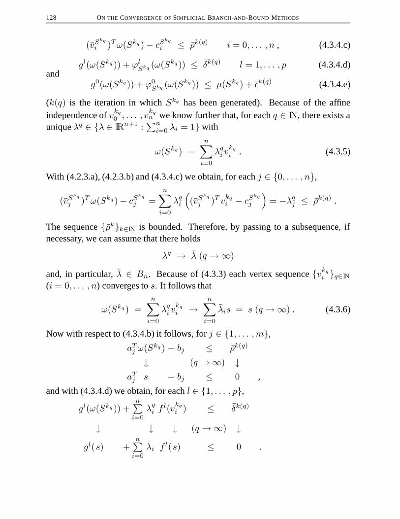
128 ON THE CONVERGENCE OFSIMPLICIAL BRANCH-AND-BOUND METHODS
(vSkq
i )Tω(Skq)− cSkq
i ≤ ρk(q) i = 0, . . . , n , (4.3.4.c)
gl(ω(Skq)) + ϕlSkq (ω(Skq)) ≤ δk(q) l = 1, . . . , p (4.3.4.d)
andg0(ω(Skq)) + ϕ0
Skq (ω(Skq )) ≤ µ(Skq) + εk(q) (4.3.4.e)
(k(q) is the iteration in whichSkq has been generated). Because of the affineindependence ofvkq
0 , . . . , vkqn we know further that, for eachq ∈ IN, there exists a
uniqueλq ∈ {λ ∈ IRn+1 :∑ni=0 λi = 1} with
ω(Skq) =n∑i=0
λqi vkq
i . (4.3.5)
With (4.2.3.a), (4.2.3.b) and (4.3.4.c) we obtain, for eachj ∈ {0, . . . , n},
(vSkq
j )Tω(Skq)− cSkq
j =n∑i=0
λqi
((vS
kq
j )T vkq
i − cSkq
j
)= −λqj ≤ ρk(q) .
The sequence{ρk}k∈IN is bounded. Therefore, by passing to a subsequence, ifnecessary, we can assume that there holds
λq → λ (q →∞)
and, in particular,λ ∈ Bn. Because of (4.3.3) each vertex sequence{vkq
i }q∈IN
(i = 0, . . . , n) converges tos. It follows that
ω(Skq) =n∑i=0
λqi vkq
i →n∑i=0
λis = s (q →∞) . (4.3.6)
Now with respect to (4.3.4.b) it follows, forj ∈ {1, . . . ,m},aTj ω(Skq) − bj ≤ ρk(q)
↓ (q →∞) ↓aTj s − bj ≤ 0 ,
and with (4.3.4.d) we obtain, for eachl ∈ {1, . . . , p},gl(ω(Skq)) +
n∑i=0
λqi fl(vkq
i ) ≤ δk(q)
↓ ↓ ↓ (q →∞) ↓gl(s) +
n∑i=0
λi fl(s) ≤ 0 .

4.3. CONVERGENCE WITH EXHAUSTIVE SUBDIVISION RULES 129
Note thatf l andgl (l ∈ {0, . . . , p}) are continuous functions (see, e.g., [ROC70,Theorem 10.1]). Therefore, we know thats is a feasible point, i.e.,F 6= ∅. Fromthe construction ofµkq = µ(Skq) (q ∈ IN) it follows that {µkq}q∈IN is a non-decreasing sequence (see Remark 4.2.2(b)), which is bounded from above by theoptimal value(f0 + g0)? <∞ of (DCP) and hence convergent to a real valueµ?.
Using (4.3.4.e) we also obtain
g0(ω(Skq)) +n∑i=0
λqi f0(vkq
i ) ≤ µ(Skq)+εk(q) ≤ (f0 + g0)?+εk(q)
↓ ↓ ↓ (q →∞) ↓ ↓ ↓g0(s) +
n∑i=0
λi f0(s) ≤ µ? + 0 ≤ (f0 + g0)?+ 0 ,
and because of the feasibility ofs there holds
g0(s) + f0(s) = (f0 + g0)? ,
showing the optimality ofs. Since the limit of a convergent sequence is unique, itfollows from (4.3.6) that
s = ω? ,
and we have proven the theorem. �
The following corollary is a direct consequence of the proof of this theorem.
COROLLARY 4.3.2. Assume thatε = δ = ρ = 0 and that an exhaustivesubdivision rule is used, then Algorithm 4.1 stops after a finite number of iterations,if no feasible point exists, i.e., ifF = ∅.
REMARK 4.3.1. If an exhaustive subdivision rule is used, it is possible toavoid nonlinear subproblems (see, for example, [HT99]). LetS = [v0, . . . , vn]be ann-simplex andxS ∈ S be an arbitrary point, e.g.,xS = 1
n+1
∑ni=0 vi.
Let further, for l ∈ {0, . . . , p}, ξlS be a subgradient ofgl at the pointxS , i.e.,ξlS ∈ ∂gl(xS), where∂gl(xS) denotes the subdifferential ofgl at the pointxS (see,e.g., [ROC70, SHO85] or Appendix B for the definition and the framework of sub-gradients and subdifferentials of convex functions). Then we know that the optimal
130 ON THE CONVERGENCE OFSIMPLICIAL BRANCH-AND-BOUND METHODS
solutionµ?(S) of the linear problem
min (ξ0S)T (x− xS) + g0(xS) + ϕ0S(x)
(ξlS)T (x − xS) + gl(xS) + ϕlS(x) ≤ 0 l = 1, . . . , p
x ∈ P ∩ S(LDCPS)
is a lower bound forminx∈F∩S[g0(x) + f0(x)
]. If we replace in the formulation
of Algorithm 4.1 the convex relaxation (DCPS) of (DCP) with respect to the sim-plexS by the linear relaxation (LDCPS), then the algorithm is still convergent (seeagain [HT99, Theorem 14]). Applying this concept to all-quadratic problems oftype (QP) leads to the lower bounds, which we used in Algorithm 3.1. Note that(LPS) and (LDCPS) coincide, ifxS is chosen asv0.
The choice between (DCPS) and (LDCPS) is a question of efficiency. The con-vex subproblems are in general harder to solve, but provide a better lower bound,since the objective function as well as the nonlinear constraints are better approx-imated. If an efficient solution method for (DCPS) is available, the use of thismethod could lead to a faster algorithm than the use of a linear problem solverfor (LDCPS) (see the numerical results in Subsection 4.6.1). Whether an efficientsolver for (DCPS) exists, depends on the special structure of this convex subprob-lem. For convex quadratic subproblems, for example, interior point methods canbe used if some additional assumptions are fulfilled (see, e.g., [JAR96]).
The previous convergence result for Algorithm 4.1 is not really surprising,since an exhaustive subdivision rule is assumed. In the next section we prove asimilar convergence result for this method in the case that theω-subdivision ruleis employed and the approach is used for solving problems of type (DCP1) and(DCP2). Recognize that theω-subdivision rule is not necessarily exhaustive.
4.4. Convergence with theω-Subdivision Rule
In this section we assume that aCONVEXSOLVER0,0,0 is known. If we ap-ply Algorithm 4.1 for solving problems of type (DCP1), we can use the Simplex-Algorithm as mentioned in Remark 4.2.1(a). For general problems of type (DCP2)such a solution method does not exist to the author’s knowledge. However, forexample in the case thatg0 is a quadratic function and thus (DCPS2 ) is a convexquadratic optimization problem with linear constraints, aCONVEXSOLVER0,0,0 isavailable (see Remark 4.2.1(b)). The existence of such a solution method for theconvex subproblems implies that we choose0-sequences for{εk}k∈IN, {δk}k∈IN

4.4. CONVERGENCE WITH THEω-SUBDIVISION RULE 131
and {ρk}k∈IN in the initialization of Algorithm 4.1, i.e.,εk = δk = ρk = 0(k ∈ IN). Furthermore, in view of Remark 4.2.2(h) we know that, for each simplexSk = [vk0 , . . . , v
kn], the optimal solutionω(Sk) of the corresponding convex sub-
problem (DCPSk
) is contained in the setSk \{vk0 , . . . , vkn}. This implies that in theused generalizedω-subdivision rule (GWSR) we choose in each iterationk ∈ INthe pointwk asω(Sk).
As a consequence of the use of aCONVEXSOLVER0,0,0 we setρ = 0, since thelinear constraints describingP are also involved in the description of the feasibleset of the subproblems (DCPS). A second consequence is that we setδ = 0, ifwe apply Algorithm 4.1 for solving problems of type (DCP1). Indeed, since theconstraints of (DCP1) are linear (p = 0), they are not relaxed in the formulationof (DCPS1 ). In this situation we know that each pointω(S) generated in Algorithm4.1 for an arbitraryn-simplexS is feasible for the original Problem (DCP1), i.e.,ω(S) ∈ F .
We assume further that in the formulation of Problem (DCP2) the functionf0
is strictly concave, i.e., for anyx, y ∈ IRn with x 6= y andλ ∈ (0, 1), there holds
f0(λx + (1− λ)y) > λf0(x) + (1− λ)f0(y) . (4.4.1)
This is not a restriction. The functionf0(x) := f0(x) − σ‖x‖22 with a real valueσ > 0 is strictly concave andg0(x) + σ‖x‖22 is still convex. Therefore, we cansolve
minx∈F
[g0(x) + f0(x)
]with a strictly concave part of the objective function instead ofmin
x∈F[g0(x) + f0(x)
].
In the following we consider the version of Algorithm 4.1, which employsonly ω-subdivisions. In order to obtain the desired convergence results for thisapproach, applied for solving problems of type (DCP1) and (DCP2), we show thatthis method is always finite, if the toleranceε is chosen greater than0, and in thecase of (DCP2), if δ is also greater than0. This proof of finiteness is based on somelemmata and corollaries whose statements are presented in the sequel. Even thoughthe pronounced results will be the same, some proofs are different depending on theproblem class which we would like to solve with Algorithm 4.1. Each proof willbe marked in a non-ambiguous way in order to clarify whether it is true for bothtypes or only for one. The longer and more technical proofs of some results will begiven in Appendix A.

132 ON THE CONVERGENCE OFSIMPLICIAL BRANCH-AND-BOUND METHODS
The proof of finiteness will be done by contradiction. The results of the follow-ing lemmata will be proven using an infinite nested sequence{Sk}k∈IN of simpliceswith the properties that, for allk ∈ IN,
Sk+1 is thedirect childof Sk = [vk0 , . . . , vkn] , (4.4.2.a)
i. e.,Sk+1 = [vk0 , . . . , vki−1, ω(Sk), vki+1, . . . , v
kn] (i ∈ {0, . . . , n}) ,
and
µk = µ(Sk) < ηk − ε . (4.4.2.b)
If the algorithm does not stop after a finite number of iterations, then – given thesequence{Sk}k∈IN of simplices which are selected in the simplex selection rule(SSR) of Algorithm 4.1 – there exists at least one subsequence with the additionalattributes (4.4.2), as it will be shown in the proof of the Finiteness Theorem 4.4.9.
If we consider, fork ∈ IN, ann-simplexSk and its direct childSk+1, then it isa known fact (see, e.g., [HPT95, Theorem 1.23] or Remark 3.2.2(c)) that, for anyx ∈ Sk+1, there holds
ϕlSk+1(x) = ϕlSk(x) + τ l(x) l = 0, . . . , p , (4.4.3)
whereτ l : IRn → IR (l ∈ {0, . . . , p}) denotes a function with nonnegative values.The following lemma specifies, for eachx ∈ Sk+1 and at least onel ∈ {0, . . . , p},a lower bound for the function valueτ l(x). This lower bound depends on thebarycentric coordinates ofx with respect toSk+1 and on the toleranceε, respec-tively δ.
LEMMA 4.4.1. LetSk be the selected simplex in iterationk ∈ IN of Algorithm4.1 withSk = [vk0 , . . . , v
ki−1, v
ki , v
ki+1, . . . , v
kn] (i ∈ {0, . . . , n}) and letS? =
[vk0 , . . . , vki−1, v?, vki+1, . . . , v
kn] be one of the simplices obtained by subdividing
Sk with respect tov? = ω(Sk).Letx be an arbitrary element ofS? with the unique representation
x = λ0vk0 + · · ·+ λiv
? + · · ·+ λnvkn ,
with λ ∈ Bn. If Sk is not fathomed in the pruning rule (PR) of Algorithm 4.1, thenthere holds
ϕ0S?(x) ≥ ϕ0
Sk(x) + ελi , if v? is (δ, 0)- feasible,
or∃l ∈ {1, . . . , p} : ϕlS?(x) ≥ ϕlSk(x) + δλi , otherwise.
(4.4.4)
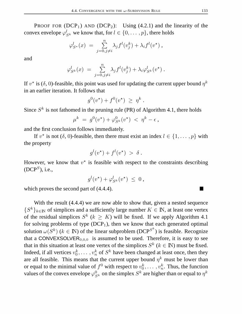
4.4. CONVERGENCE WITH THEω-SUBDIVISION RULE 133
PROOF FOR(DCP1) AND (DCP2): Using (4.2.1) and the linearity of theconvex envelopeϕlSk we know that, forl ∈ {0, . . . , p}, there holds
ϕlS?(x) =n∑
j=0,j 6=iλjf
l(vkj ) + λifl(v?) ,
and
ϕlSk(x) =n∑
j=0,j 6=iλjf
l(vkj ) + λiϕlSk(v?) .
If v? is (δ, 0)-feasible, this point was used for updating the current upper boundηk
in an earlier iteration. It follows that
g0(v?) + f0(v?) ≥ ηk .
SinceSk is not fathomed in the pruning rule (PR) of Algorithm 4.1, there holds
µk = g0(v?) + ϕ0Sk(v?) < ηk − ε ,
and the first conclusion follows immediately.If v? is not (δ, 0)-feasible, then there must exist an indexl ∈ {1, . . . , p} with
the property
gl(v?) + f l(v?) > δ .
However, we know thatv? is feasible with respect to the constraints describing(DCPS), i.e.,
gl(v?) + ϕlSk(v?) ≤ 0 ,
which proves the second part of (4.4.4). �
With the result (4.4.4) we are now able to show that, given a nested sequence{Sk}k∈IN of simplices and a sufficiently large numberK ∈ IN, at least one vertexof the residual simplicesSk (k ≥ K) will be fixed. If we apply Algorithm 4.1for solving problems of type (DCP1), then we know that each generated optimalsolutionω(Sk) (k ∈ IN) of the linear subproblem (DCPS
k
) is feasible. Recognizethat aCONVEXSOLVER0,0,0 is assumed to be used. Therefore, it is easy to seethat in this situation at least one vertex of the simplicesSk (k ∈ IN) must be fixed.Indeed, if all verticesvk0 , . . . , v
kn of Sk have been changed at least once, then they
are all feasible. This means that the current upper boundηk must be lower thanor equal to the minimal value off0 with respect tovk0 , . . . , v
kn. Thus, the function
values of the convex envelopeϕ0Sk on the simplexSk are higher than or equal toηk

134 ON THE CONVERGENCE OFSIMPLICIAL BRANCH-AND-BOUND METHODS
(compare with (4.2.1)), and the simplexSk must be fathomed in the pruning rule(PR) of Algorithm 4.1 (see also the proof of Lemma 4.7.1).
In order to prove that one vertex must be fixed in the case of (DCP2) we needmore technical effort, sinceω(Sk) is not necessarily (δ, 0)-feasible. However, ap-plying this necessary effort, we obtain a stronger result. We are able to show thatthe nested simplex sequence shrinks to a lower-dimensional simplexS, whereSis given by the fixed vertices of the residual simplicesSk (k ≥ K). In Lemma4.4.2 this stronger result is formulated and the corresponding proof is presented inSection A.1. In this proof we do not use the strict concavity off0. Thus, this proof,and consequently the following lemma, is also valid in the case of (DCP1).
LEMMA 4.4.2. Let{Sk}k∈IN be an infinite nested sequence of simplices gen-erated by Algorithm 4.1 with Properties (4.4.2). Then there exist a numberK ∈ INand an integerr with 0 ≤ r < n such that, for eachk ≥ K, there holds
Sk = [v0, . . . , vr, vkr+1, . . . , vkn] , (4.4.5)
wherev0, . . . , vr are fixed vectors, whilevkr+1, . . . , vkn (k ∈ IN, k ≥ K) change
infinitely often. Moreover, there holds⋂k∈IN
Sk = [v0, . . . , vr] =: S . (4.4.6)
In order to show that the numberr of fixed vertices of the residual simplicesSk
(k ≥ K) must be greater than1, i.e.,r ≥ 1, we first prove that each accumulationpoint of the sequence{ω(Sk)}k∈IN is contained in the setS \ {v0, . . . , vr}. Thisis the result of the following lemma. The proof of this lemma, which also does notdepend on the considered problem class, is given in Section A.2.
LEMMA 4.4.3. Let{Sk}k∈IN be an infinite nested sequence of simplices gen-erated by Algorithm 4.1 with Properties (4.4.2). LetK ∈ IN and0 ≤ r < n begiven by Lemma 4.4.2. Denote byS = [v0, . . . , vr] the fixed face of the residualsimplices
Sk = [v0, . . . , vr, vkr+1, . . . , vkn] (k ≥ K) .
Then, for each accumulation pointω of the sequence{ω(Sk)}k∈IN, there holds
ω ∈ S \ {v0, . . . , vr} . (4.4.7)
4.4. CONVERGENCE WITH THEω-SUBDIVISION RULE 135
This result will also be helpful in the proof of the next Lemma 4.4.5. However,a direct consequence of the previous result is that at least two vertices of the residualsimplicesSk (k ≥ K) have to be fixed.
COROLLARY 4.4.4. Let {Sk}k∈IN be an infinite nested sequence generatedby Algorithm 4.1 with Properties (4.4.2). Let furtherK ∈ IN and0 ≤ r < n begiven by Lemma 4.4.2. Then there holds
r ≥ 1 . (4.4.8)
PROOF FOR(DCP1) AND (DCP2): Assume, by contradiction, that thereholdsr = 0, i.e.,
S = {v0} =⋂k∈IN
Sk .
The sequence{ω(Sk)}k∈IN is bounded. Therefore there exists an accumulationpoint ω of this sequence. Since the simplex sequence{Sk}k∈IN consists of nested,compact and non-empty sets, it follows
ω ∈ S = {v0} .
This is a contradiction to the result of Lemma 4.4.3, and hence we obtainr ≥ 1. �
REMARK 4.4.1. The result of the previous corollary follows also by the con-siderations regarding an exhaustive subdivision rule in Section 4.3. Indeed, if weare in the situation that only one vertex of the simplex sequence{Sk}k≥K is fixed,then it follows by Lemma 4.4.2 that there holds
S = {v0} =⋂k∈IN
Sk . (4.4.9)
This relation is the essential part in the proof of Theorem 4.3.1, which guaranteesthe convergence of Algorithm 4.1 for an exhaustive subdivision rule. Therefore, bythe same argumentation as in the corresponding proof (see Section 4.3) we wouldobtain finiteness of Algorithm 4.1 forε, δ > 0, if (4.4.9) is satisfied.
In order to prove finiteness of the variant of Algorithm 4.1, which employs onlyω-subdivisions, it is not sufficient that each accumulation pointω of the sequence{ω(Sk)}k∈IN is contained in the set[v0, . . . , vr] \ {v0, . . . , vr}. Actually, we needa slightly stronger result. The next lemma signifies that the barycentric coordinatesof ω(Sk) (k ≥ K) with respect to the not-fixed vertices ofSk (k ≥ K) converge

136 ON THE CONVERGENCE OFSIMPLICIAL BRANCH-AND-BOUND METHODS
to 0. The proofs of this lemma, which are different for the considered problemclasses, are given in Section A.3.
LEMMA 4.4.5. Let{Sk}k∈IN be an infinite nested sequence generated by Al-gorithm 4.1 with Properties (4.4.2). LetK ∈ IN and1 ≤ r < n be chosen as inLemma 4.4.2 and let
ω(Sk) =r∑i=0
λki vi +n∑
i=r+1
λki vki , (4.4.10)
with λk ∈ Bn andk ≥ K. Then there holds
Λk :=n∑
i=r+1
λki −→ 0 (k →∞) . (4.4.11)
It follows immediately from the previous lemma that, for eachk ≥ K, theoptimal solutionω(Sk) of the linear subproblem (DCPS1 ) can be represented asa combination of a pointxk, contained in the fixed faceS = [v0, . . . , vr] of thesimplicesSk, and a residualςk ∈ IRn. This representation is given in the followingcorollary. Furthermore, it is shown that the distance between the function values ofϕ0Sk at the pointsω(Sk) andxk converges to0.
COROLLARY 4.4.6. Let {Sk}k∈IN be an infinite nested sequence generatedby Algorithm 4.1 with Properties (4.4.2), and letK ∈ IN and1 ≤ r < n be givenby Lemma 4.4.2. Then there exists a numberK ∈ IN with K ≥ K such that,for eachk ≥ K, there exist a pointxk ∈ [v0, . . . , vr], a point ςk ∈ IRn with‖ςk‖2 → 0 (k →∞) and a real valueσk with σk → 0 (k →∞) satisfying
ω(Sk) = xk + ςk (4.4.12)
and
ϕ0Sk(ω(Sk)) = ϕ0
Sk(xk) + σk . (4.4.13)
PROOF FOR(DCP1) AND (DCP2): In view of Relation (4.4.11) we knowthat there exists an integerK ≥ K such that, for eachk ≥ K, there holds
Λk < 1 .
Set, fork ≥ K,
xk :=r∑i=0
λki1− Λk
vi

4.4. CONVERGENCE WITH THEω-SUBDIVISION RULE 137
with λk ∈ Bn andΛk ∈ IR defined as in (4.4.10) and (4.4.11). Obviously thereholdsxk ∈ [v0, . . . , vr], and we obtain the following representation ofω(Sk)
ω(Sk) = xk +n∑
i=r+1
λki vki − Λk
r∑i=0
λki1− Λk
vi︸ ︷︷ ︸=: ςk
.
For the function value ofϕ0Sk at the pointω(Sk) we further get
ϕ0Sk(ω(Sk)) = ϕ0
Sk(xk) +n∑
i=r+1
λki f0(vki )− Λk
r∑i=0
λki1− Λk
f0(vi)︸ ︷︷ ︸=: σk
.
Because of the boundedness ofS0, there exist real valuesC > 0 andD > 0 suchthat, for eachx ∈ S0, there holds‖x‖2 ≤ C and|f0(x)| ≤ D. With Lemma 4.4.5it follows
‖ςk‖2 = ‖n∑
i=r+1
λki vki − Λkxk‖2 ≤ 2ΛkC → 0 (k →∞) .
Furthermore, we obtain
|σk| = |n∑
i=r+1
λki f0(vki )− Λk
r∑i=0
λki1− Λk
f0(vi)|
≤ ΛkD + Λkr∑i=0
λki1− Λk︸ ︷︷ ︸= 1
D → 0 (k →∞) .
�
By using all previous results it is now possible to prove that there exists anumberK ≥ K such that, for eachk ≥ K, we are able to replace the pointxk ∈ S = [v0, . . . , vr] in Relation (4.4.12) by a pointrk ∈ S with the propertythat a lower bound forµk = µ(Sk) depending onrk can be given. This lowerbound is the sum of the function valueg0(rk) + ϕ0
Sk(rk) of the objective func-
tion of Problem (DCPSk
) and a residual part depending onΛk, which convergesto 0 – with respect toΛk – slower than the Euclidean distance between the pointsω(Sk) andrk. This is the result of the following Lemma 4.4.7 and will be essen-tial for the proof of finiteness of the version of Algorithm 4.1, which employs only

138 ON THE CONVERGENCE OFSIMPLICIAL BRANCH-AND-BOUND METHODS
ω-subdivisions. The proofs of this lemma, which are again different for both prob-lem classes, are given in Section A.4. The notationo(x) is used for an arbitraryfunctionτ : IR→ IR with the property
τ(x)x→ 0 (x→ 0) .
LEMMA 4.4.7. Let {Sk}k∈IN be an infinite nested simplex sequence gener-ated by Algorithm 4.1 with Properties (4.4.2). Then there exist a numberK ∈ IN, a real valueσ > 0 and, for eachk ≥ K, a point rk ∈ [v0, . . . , vr]satisfying
g0(ω(Sk)) + ϕ0Sk(ω(Sk)) ≥ g0(rk) + ϕ0
Sk(rk) + σΛk + o(Λk) , (4.4.14.a)
ϕlSk(rk) ≤ o(Λk) l = 1, . . . , p (4.4.14.b)and
‖ω(Sk)− rk‖2 = o(Λk) (4.4.14.c)
with Λk (k ≥ K) defined as in (4.4.11).
In order to obtain a contradiction in the proof of the final finiteness result it isstill not sufficient that for eachk ≥ K we have got a pointrk ∈ S = [v0, . . . , vr]with Properties (4.4.14.a)-(4.4.14.c). Beyond it, we need a pointrk ∈ S withProperties (4.4.14.a) and (4.4.14.c), which is, additionally, feasible with respect tothe convex subproblem (DCPS
k
). Thus, it is necessary to prove the existence of apoint rk satisfying (4.4.14.a), (4.4.14.c) and
rk ∈ P , ϕlSk(rk) ≤ 0 l = 1, . . . , p . (4.4.15)
Since the convex envelopesϕlSk (l = 1, . . . , p, k ≥ K) have, in view of the resultof Lemma 4.4.2, the same function values onS independent ofk, it follows, foreachx ∈ S andk ≥ K,
ϕlSk(x) =r∑i=0
λifl(vi)
with λ ∈ Br, x =∑ri=0 λivi. Therefore, Condition (4.4.15) is fulfilled, ifrk is
contained in the set
F := {x ∈ P ∩ S :∑r
i=0λifl(vi) ≤ 0 , l = 1, . . . , p
with λ ∈ Br , x =∑ri=0λivi} .
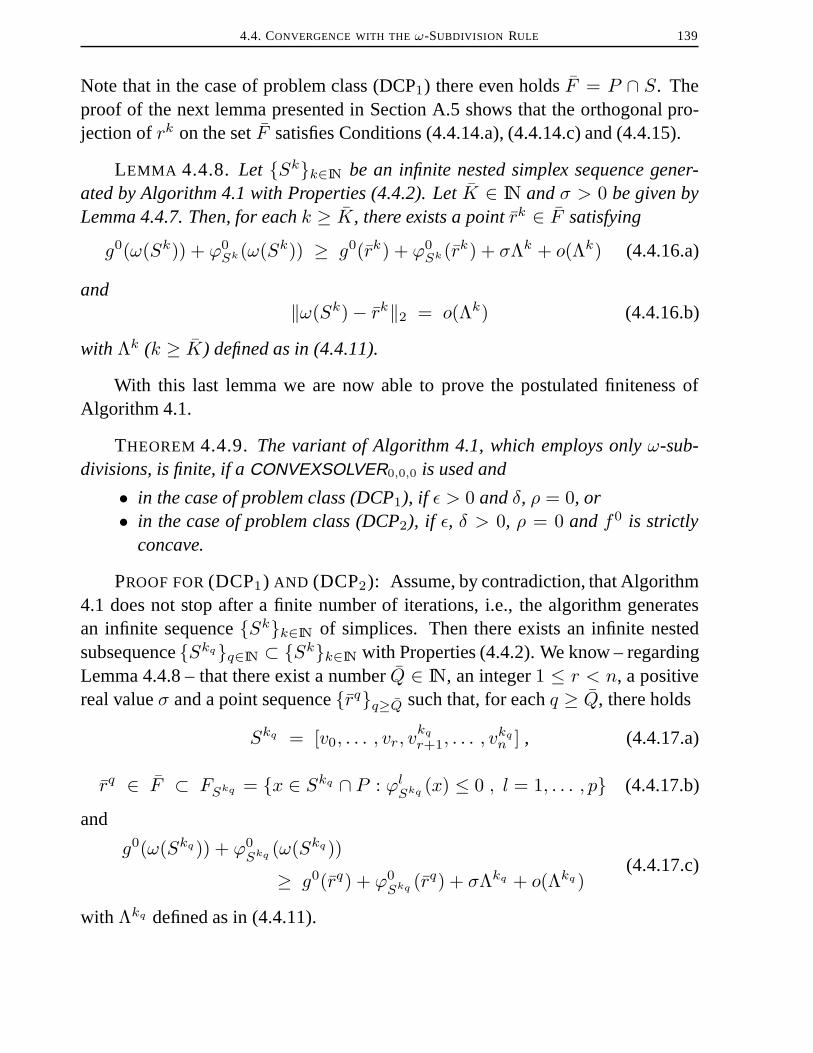
4.4. CONVERGENCE WITH THEω-SUBDIVISION RULE 139
Note that in the case of problem class (DCP1) there even holdsF = P ∩ S. Theproof of the next lemma presented in Section A.5 shows that the orthogonal pro-jection ofrk on the setF satisfies Conditions (4.4.14.a), (4.4.14.c) and (4.4.15).
LEMMA 4.4.8. Let {Sk}k∈IN be an infinite nested simplex sequence gener-ated by Algorithm 4.1 with Properties (4.4.2). LetK ∈ IN andσ > 0 be given byLemma 4.4.7. Then, for eachk ≥ K, there exists a pointrk ∈ F satisfying
g0(ω(Sk)) + ϕ0Sk(ω(Sk)) ≥ g0(rk) + ϕ0
Sk(rk) + σΛk + o(Λk) (4.4.16.a)
and‖ω(Sk)− rk‖2 = o(Λk) (4.4.16.b)
with Λk (k ≥ K) defined as in (4.4.11).
With this last lemma we are now able to prove the postulated finiteness ofAlgorithm 4.1.
THEOREM 4.4.9. The variant of Algorithm 4.1, which employs onlyω-sub-divisions, is finite, if aCONVEXSOLVER0,0,0 is used and
• in the case of problem class (DCP1), if ε > 0 andδ, ρ = 0, or• in the case of problem class (DCP2), if ε, δ > 0, ρ = 0 andf0 is strictly
concave.
PROOF FOR(DCP1) AND (DCP2): Assume, by contradiction, that Algorithm4.1 does not stop after a finite number of iterations, i.e., the algorithm generatesan infinite sequence{Sk}k∈IN of simplices. Then there exists an infinite nestedsubsequence{Skq}q∈IN ⊂ {Sk}k∈IN with Properties (4.4.2). We know – regardingLemma 4.4.8 – that there exist a numberQ ∈ IN, an integer1 ≤ r < n, a positivereal valueσ and a point sequence{rq}q≥Q such that, for eachq ≥ Q, there holds
Skq = [v0, . . . , vr, vkq
r+1, . . . , vkqn ] , (4.4.17.a)
rq ∈ F ⊂ FSkq = {x ∈ Skq ∩ P : ϕlSkq (x) ≤ 0 , l = 1, . . . , p} (4.4.17.b)
and
g0(ω(Skq)) + ϕ0Skq (ω(Skq))
≥ g0(rq) + ϕ0Skq (rq) + σΛkq + o(Λkq )
(4.4.17.c)
with Λkq defined as in (4.4.11).

140 ON THE CONVERGENCE OFSIMPLICIAL BRANCH-AND-BOUND METHODS
The pointω(Skq) is the optimal solution of the convex optimization problem
minx∈F
Skq
[g0(x) + ϕ0
Skq (x)]
.
Therefore, it follows from the feasibility ofrq with respect to the setFSkq (see(4.4.17.b)) that
g0(ω(Skq)) + ϕ0Skq (ω(Skq )) ≤ g0(rq) + ϕ0
Skq (rq) , (4.4.18)
and from (4.4.17.c) we obtain, forq ≥ Q,
g0(rq) + ϕ0Skq (rq) ≥ g0(rq) + ϕ0
Skq (rq) + σΛkq + o(Λkq ) .
This relation is equivalent to
σΛkq︸ ︷︷ ︸≥0
+o(Λkq ) ≤ 0 .
Considering Lemma 4.4.5 we know that the sequence{Λkq}q∈IN converges to0, if q tends to infinity, and, furthermore, this sequence converges slower than{o(Λkq)}q∈IN to 0. Thus, there must exist a numberq′ ≥ Q satisfying
Λkq′ = 0 . (4.4.19)
Indeed, ifΛkq is always greater than0, it follows by definition ofo(Λ) that
σ + o(Λkq )
Λkq≤ 0
↓ (q →∞)
0 < σ+ 0 ≤ 0 ,
which is a contradiction.Relation (4.4.19) is only possible if there holds
ω(Skq′ ) ∈ [v0, . . . , vr] .
If ω(Skq′ ) is contained in[v0, . . . , vr] \ {v0, . . . , vr}, Skq′+1 will be generatedby replacing one of the verticesv0, . . . , vr. However, this contradicts Property(4.4.17.a) of the simplex sequence{Skq}q∈IN. Thus, there holds
ω(Skq′ ) ∈ {v0, . . . , vr} (4.4.20.a)
and, additionally,
ϕlS
kq′ (ω(Skq′ )) = f l(ω(Skq′ )) l = 0, . . . , p . (4.4.20.b)

4.4. CONVERGENCE WITH THEω-SUBDIVISION RULE 141
The pointω(Skq′ ) ∈ Skq′ ∩ P is feasible with respect to the convex optimization
problem (DCPSk
q′ ). In view of (4.4.20.b) we obtain
f l(ω(Skq′ )) = ϕlS
kq′ (ω(Skq′ )) ≤ 0 l = 1, . . . , p ,
and therefore we know thatω(Skq′ ) is a (δ, 0)-feasible point of Problem (DCPi)(i = 1, 2). Hence, the pointω(Skq′ ) was used for updating the upper bound, and itfollows
µkq′ = µ(Skq′ ) = g0(ω(Skq′ )) + ϕ0
Sk
q′ (ω(Skq′ ))
≤ ηkq′ ≤ g0(ω(Skq′ )) + f0(ω(Skq′ )) .
In view of Relation (4.4.20.b) withl = 0 we obtain
µkq′ = ηkq′ ,
contradicting, forε > 0, Property (4.4.2.b) of the simplex sequence{Skq}q∈IN andcompleting the proof. �
This finiteness result guarantees the convergence of Algorithm 4.1 only em-ployingω-subdivisions, applied for solving problems of type (DCP1) and (DCP2).However, the convergence of Algorithm 4.1 does not hold in the sense of Theorem4.3.1, i.e., we do not know whether each accumulation pointω? of the point se-quence{ω(Sk)}k∈IN is optimal, if Algorithm 4.1 withε = δ = ρ = 0 generatesan infinite sequence{Sk}k∈IN of simplices. From Theorem 4.4.9 we obtain forproblem class (DCP1) that, if ε is also chosen as0, then there holds
µk = µ(Sk) → minx∈P
f0(x) (k →∞) (4.4.21)
in the infinite case. Note thatP is assumed to be non-empty and that{µ(Sk)}k∈IN
is by construction non-decreasing. For this problem class we obtain, furthermore,that each accumulation pointx?f of the sequence{xkf}k∈IN is optimal for (DCP1),wherexkf denotes the best known point at iterationk ∈ IN, i.e., ηk = f0(xkf ).Thus, in this case there holds a similar convergence result as in Theorem 4.3.1.
In the case of problems of type (DCP2) we obtain from Theorem 4.4.9 con-vergence of Algorithm 4.1 only in the following sense. For arbitrary accuraciesε, δ > 0 we know that this method detects in finite either the emptiness ofF or an(ε, δ, 0)-solution of Problem (DCP2). This implies that, ifF 6= ∅, we are able toconstruct a sequence{xk}k∈IN such that each accumulation point of this sequence

142 ON THE CONVERGENCE OFSIMPLICIAL BRANCH-AND-BOUND METHODS
is an optimal solution of (DCP2). This can be done by successively applying Algo-rithm 4.1 with different positive accuraciesεk, δk (k ∈ IN) belonging to sequences{εk}k∈IN, {δk}k∈IN converging to0. Such an iterative application of Algorithm4.1 detects in particular the emptiness ofF in finite time (compare with Corollary4.3.2).
REMARK 4.4.2. At first glance the above convergence results for the variantof Algorithm 4.1, which employs onlyω-subdivisions and is applied for the solu-tion of problems of type (DCP1) and (DCP2), are weaker than the one obtainedin the exhaustive case (Theorem 4.3.1) – especially the result for problem class(DCP2). However – from a practical point of view – these different convergenceconcepts have the same quality. Note that the stronger convergence of algorithms inthe sense of Theorem 4.3.1 is only needed in order to obtain finiteness of such ap-proaches, when approximate solutions are sufficient. Hence, both results show thatAlgorithm 4.1 with an exhaustive subdivision rule as well as withω-subivisions isfinite, if we are satisfied with (ε, δ, 0)-solutions of Problem (DCP2) (ε, δ > 0). Thisis the essential result we need in order to apply this method in practice.
As the counterexample in the next section shows, it is not possible to extendthe presented proof techniques in order to ensure the convergence of Algorithm4.1 – in the above sense – in the general case. However, a careful checking ofthe proofs shows that all results until Lemma 4.4.7 are also provable in the caseof the general problem class (DCP3). Moreover, using aCONVEXSOLVERεk,δk,0
(k ∈ IN) with non-increasing sequences{εk}k∈IN and{δk}k∈IN converging to0instead of aCONVEXSOLVER0,0,0 , it is also possible to verify all these results.However, in this situation it is necessary to change slightly the formulation of someof these lemmata, where these changes do not alter the essential content of theresults. For example, the result of Lemma 4.4.1 does not hold for eachk ∈ IN. It isonly provable that there exists aK ∈ IN such that Relation (4.4.4) withε2λi insteadof ελi and δ2λi instead ofδλi is true, for eachk ≥ K.
Before presenting the counterexample we would like to give some ideas in or-der to understand, why the proofs fail in the general case. It is immediately clear,that the Finiteness Theorem 4.4.9 cannot be proven using aCONVEXSOLVERεk,δk,0.
Indeed, without an exact solution of the convex subproblem (DCPSk
) the relation(4.4.18) is not fulfilled, and we are not able to derive the contradiction. This em-phasizes that the assumption of aCONVEXSOLVER0,0,0 is substantial for the proofof Theorem 4.4.9.

4.4. CONVERGENCE WITH THEω-SUBDIVISION RULE 143
Apart from the problem that it is not reasonable to assume that aCONVEX-SOLVER0,0,0 is available in the case of problems of type (DCP3), the attempt ofproving the presented finiteness result in this case even fails in the proof of Lemma4.4.8. We show there (see Appendix A) that the orthogonal projectionrk of rk onthe set
F := {x ∈ P ∩ S :∑r
i=0λifl(vi) ≤ 0 , l = 1, . . . , p
with λ ∈ Br , x =∑r
i=0λivi}has the property‖rk − rk‖2 = o(Λk) and, thus, we can derive that this point sat-isfies the required conditions of Lemma 4.4.8. We prove this property by usingthe Karush-Kuhn-Tucker(KKT)-conditions (see, e.g., [HOR79, FLE87, MAN94])for the convex optimization problemminx∈F ‖x − rk‖22. Since this problem hasonly linear constraints we do not need a regularity condition for applying the KKT-theory. If we try to use the same argumentation in the case of problem class (DCP3)with continuous differentiable functionsgl (l ∈ {1, . . . , p}), then we need a regu-larity condition for the convex optimization problemminx∈F3
‖x− rk‖22 with
F3 := {x ∈ P ∩ S : gl(x) +∑r
i=0λifl(vi) ≤ 0 , l = 1, . . . , p
with λ ∈ Br , x =∑r
i=0λivi} ,
since this problem has also nonlinear convex constraints. In general, we are not ableto assume that such a regularity condition is fulfilled for each possible simplexS =[v0, . . . , vr]. The counterexample presented in the next section shows a situationwhere the KKT-conditions fail.
Even if we would be able to formulate a condition checkable in advance forproblems of type (DCP3) ensuring the applicability of the KKT-theory, anotherproblem occurs. Apart from the application of the KKT-conditions a second es-sential part in the proof of Lemma 4.4.8 is the existence of a positive real valueτ independent of the iteration counterk (see Relation (A.5.16) in Section A.5).The existence of this value depends on the fact that there is only a finite numberof possible gradients in the formulation of the KKT-conditions for the problemsminx∈F ‖x− rk‖22 (k ∈ IN). Formulating these conditions forminx∈F3
‖x− rk‖22with continuous differentiable functionsgl (l = 0, . . . , p) we can obtain in eachiteration gradients depending on∇gl(rk) (l ∈ {1, . . . , p}). Therefore, the set ofpossible gradients is no longer finite, and the existence of the necessary valueτ > 0is in general not provable, at least not provable with the used techniques.

144 ON THE CONVERGENCE OFSIMPLICIAL BRANCH-AND-BOUND METHODS
4.5. A Counterexample
In this section we show that the variant of Algorithm 4.1, which employsonly ω-subdivisions, can fail, if this approach is used for solving problems of type(DCP3). Consider the following optimization problem
min f(xy
)14x
2 + y2 ≤ 1
g(x) + y2 ≤ 1(xy
) ∈ P ⊂ IR2
(CE)
with f : IR2 → IR, f(xy
)= −‖(xy)‖22 = −x2 − y2 , g : IR→ IR
g(x) ={
0 , if x ≥ 0x2 , otherwise
andP = {(xy) ∈ IR2 : x ≥ −1 , − 12x + y ≥ − 3
2 , −x − y ≥ −3}. The functionf is concave, in particular strictly concave, the nonlinear constraint functions areobviously convex andP is a full-dimensional, non-empty polytope. Therefore, theProblem (CE) belongs to the class (DCP3) and the feasible region of (CE) is givenby
F = {(xy) ∈ P : 14x
2 + y2 ≤ 1 , g(x) + y2 ≤ 1}(see Figure 4.1). It is easy to see that the functionf attains its unique minimum onF at the point
(x?
y?
)=(20
)with optimal valuef? = −4.
In the following we apply the variant of Algorithm 4.1, which employs onlyω-subdivisions, for solving Problem (CE). We will see that even withε > 0 anda CONVEXSOLVER0,0,0 this approach generates an infinite sequence{Sk}k∈IN ofsimplices with the properties that, for eachk ∈ IN, there holds
µ(Sk) < −9 , (4.5.1.a)
f(ω(Sk)) = −1 (4.5.1.b)and (
x?
y?
)/∈ Sk . (4.5.1.c)
Since the functionf is continuous it follows that each accumulation pointω? of thesequence{ω(Sk)}k∈IN has the function valuef(ω?) = −1. Thus, we know that

4.5. A COUNTEREXAMPLE 145
FIGURE 4.1. The feasible setF of Problem (CE)
Fv0
v2
(x?
y?
)
v1
y
x
ω? is not optimal. This shows that this variant of Algorithm 4.1 is not convergentin the sense of Theorem 4.3.1. Moreover, if the accuraciesδ, ρ > 0 are chosensufficiently small, we are able to guarantee that there holds
minx∈Fδ,ρ
f(xy
) ≥ −5
with Fδ,ρ = {(xy) ∈ IR2 : 14x
2 + y2 ≤ 1 + δ , g(x) + y2 ≤ 1 + δ ,
−x ≤ 1 + ρ , 12x − y ≤ 3
2 + ρ , x + y ≤ 3 + ρ}. This implies that inAlgorithm 4.1 the upper boundηk (k ∈ IN) is always not smaller than−5, andfrom Property (4.5.1.a) of the lower bound sequence we know that forε ∈ (0, 4)Algorithm 4.1 does not terminate after a finite number of iterations. Hence, thisapproach is also not convergent in the sense of Theorem 4.4.9.
The polytopeP is a 2-simplex with the verticesv0 =(30
), v1 =
(−1−2
)and
v2 =(−1
4
)(see Figure 4.1). Thus, we can chooseP as the start-simplexS0, i.e.,
S0 = [v0, v1, v2]. In view of (4.2.2) we obtain for the convex envelopeϕS0 of f on

146 ON THE CONVERGENCE OFSIMPLICIAL BRANCH-AND-BOUND METHODS
the setS0 the following relation
ϕS0
(xy
)= 0 · (x− 3) + (−2) · (y − 0)︸ ︷︷ ︸
=(ζS0 )T
((xy
)−v0) + (−9)︸︷︷︸
=f(v0)
.
It follows immediately that the optimal solution ofminz∈F ϕS0(z) is the pointω(S0) =
(01
)with optimal valueϕS0(ω(S0)) = −11. Thus we getµ0 = −11 and
f(ω(S0)) = −1, and the simplexS0 is subdivided – using theω-subdivision rule– in the three simplices
S01 = [v0, v1, ω(S0)] ,
S02 = [v0, ω(S0), v2]
and
S03 = [ω(S0), v1, v2]
(see Figure 4.2(a)).
FIGURE 4.2. Subdivision ofS0 with respect toω(S0)
v0
v1
S01
S03
S02
ω(S0)
v2
(a)
v0
v2
w
S02
S02
ω(S0)
(b)

4.5. A COUNTEREXAMPLE 147
We prove now that the following relations hold
min{µ(S01), µ(S0
2)} ≥ −9 (4.5.2)and
µ(S03) < −9 , (4.5.3)
which means thatS03 is chosen as the new simplexS1 at the end of iteration0.
Because ofmin{f(v0), f(v1), f(ω(S0))} = min{−9,−5,−1} = −9 it is obviousthat, for eachz ∈ S0
1 , ϕS01(z) ≥ −9 and henceµ(S0
1) ≥ −9. In order to provethis relation forS0
2 we need more effort. Using again the representation (4.2.2) forconvex envelopes we obtain
ϕS02
(xy
)= −5x− 7y + 6 .
The pointw =(−0.5
2.5
)= 0.5ω(S0) + 0.5v2 belongs to the edge[ω(S0), v2] of
the simplexS02 and has the function valueϕS0
2(w) = −9. The simplexS0
2 can bepartitioned into two simplices
S02 = [v0, ω(S0), w] and S0
2 = [v0, w, v2]
(see Figure 4.2(b)), with the properties
ϕS02(z) ≥ −9 ∀z ∈ S0
2and
ϕS02(z) ≤ −9 ∀z ∈ S0
2 .
Since the simplexS02 does not contain a feasible point of Problem (CE), i.e.,
F ∩ S02 = ∅ (see again Figure 4.2(b)), we obtainµ(S0
2 ) ≥ −9, which provesRelation (4.5.2).
Denote now for a pointw =(wx
wy
) ∈ {(xy) ∈ IR2 : x2 + y2 = 1 , −1 < x ≤ 0 ,0 < y ≤ 1} ⊂ F by
F (w) := {(xy) ∈ IR2 : x2 + y2 = 1 , −1 < x < wx , 0 < y < wy}the part of the boundary of the feasible regionF of (CE) which lies between thepoints
(−10
)and
(wx
wy
). We verify Relation (4.5.3) by showing that the optimal
solution of minz∈F∩S0
3
ϕS03(z) must be attained at a pointw ∈ F (ω(S0)) with the
property
ϕS03(w) < −9 . (4.5.4)
This will be done by the next lemma. However, this lemma presents a more generalresult, which will also be helpful in the sequel.

148 ON THE CONVERGENCE OFSIMPLICIAL BRANCH-AND-BOUND METHODS
LEMMA 4.5.1. Let w be a point on the part{(xy) ∈ IR2 : x2 + y2 = 1 ,−1 < x ≤ 0 , 0 < y ≤ 1} of the boundary of the feasible regionF of Problem(CE). LetS(w) be the2-simplex with the verticesw, v1 =
(−1−2
)andv2 =
(−14
)(see Figure 4.3) and letϕS(w) : IR2 → IR be the convex envelope off on the setS(w) = [w, v1, v2]. Let furtherw be the optimal solution of min
z∈F∩S(w)ϕS(w)(z).
Then there holds
w ∈ F (w) (4.5.5.a)and
ϕS(w)(w) < −9 . (4.5.5.b)
FIGURE 4.3. Situation in Lemma 4.5.1
��������������������
��������������������
S(w)
v2
w
F (w)v1
y
x
PROOF: From (4.2.2) we know thatϕS(w)
(xy
)((xy
) ∈ IR2) is given by
ϕS(w)
(xy
)= 2 ba (x − wx) + (−2)(y − wy)− 1
with w =(wx
wy
), b = 4 + wy anda = 1 + wx. Consider the set
F := F (w) ∩{(
τ√1−τ2
): −1 < τ ≤ −b√
a2+b2
}.
Because ofwx > −1 we obtaina > 0 and, therefore, −b√a2+b2
> −1. It follows
that the setF is not empty and, moreover, there holdsF ⊂ S(w) ∩ F (note thatF (w) ⊂ S(w), see Figure 4.3). Showing, for allw ∈ F , the relation
ϕS(w)(w) < −9 , (4.5.6)

4.5. A COUNTEREXAMPLE 149
we will obtain that the minimal value ofϕS(w) on the setS(w) ∩ F must be lowerthan−9. For this aim consider the one-dimensional functionϕS(w) : [−1, 0]→ IR,
ϕS(w)(τ) := ϕS(w)
(τ√
1−τ2
).
There holdsϕS(w)(−1) = −9. Therefore, in order to prove Relation (4.5.6) it issufficient to show that the functionϕS(w) is monotonously decreasing along theline between−1 and −b√
a2+b2. The functionϕS(w) is obviously differentiable in
each pointτ ∈ (−1, 0), and there holds
∂ϕS(w)(τ)∂τ
= 2b
a+
2τ√1− τ2
.
For τ ∈ (−1, −b√a2+b2
) we know that1 − τ2 ≤ 1 − b2
a2+b2 = a2
a2+b2 and, thus,because ofτ < 0 we obtain
2τ√1− τ2
≤ 2τa√
a2+b2
< 2−b√a2+b2
a√a2+b2
= −2ba
.
It follows that, for eachτ ∈ (−1, −b√a2+b2
), there holds
∂ϕS(w)(τ)∂τ
< 0 ,
which shows thatϕS(w) is monotonously decreasing on(−1, −b√a2+b2
) and, thus,
there holdsϕS(w)(w) < −9, i.e., Relation (4.5.5.b) is fulfilled.In order to prove Relation (4.5.5.a) assume, by contradiction, that there holds
w /∈ F (w). Because of the structure of the setF ∩ S(w) (see the shaded region inFigure 4.3) we know that, for each pointw ∈ (F ∩ S(w)) \ (F (w) ∪ {w, (−1
0
)}),the line betweenw andv2 must intersect the setF (w). Because ofϕS(w)(w) < −9we havew /∈ {w, (−1
0
)}. Let w be the intersection point of[w, v2] andF (w). Itfollows that there is a real valueλ ∈ (0, 1) with w = w+λ(v2− w) and we obtain
ϕS(w)(w) = ϕS(w)(w) + λ
2ba
(−1− wx)︸ ︷︷ ︸<0,wx∈(−1,0]
−2 (4− wy)︸ ︷︷ ︸>0,wy∈[−1,1]
< ϕS(w)(w)
contradicting the optimality ofw. �
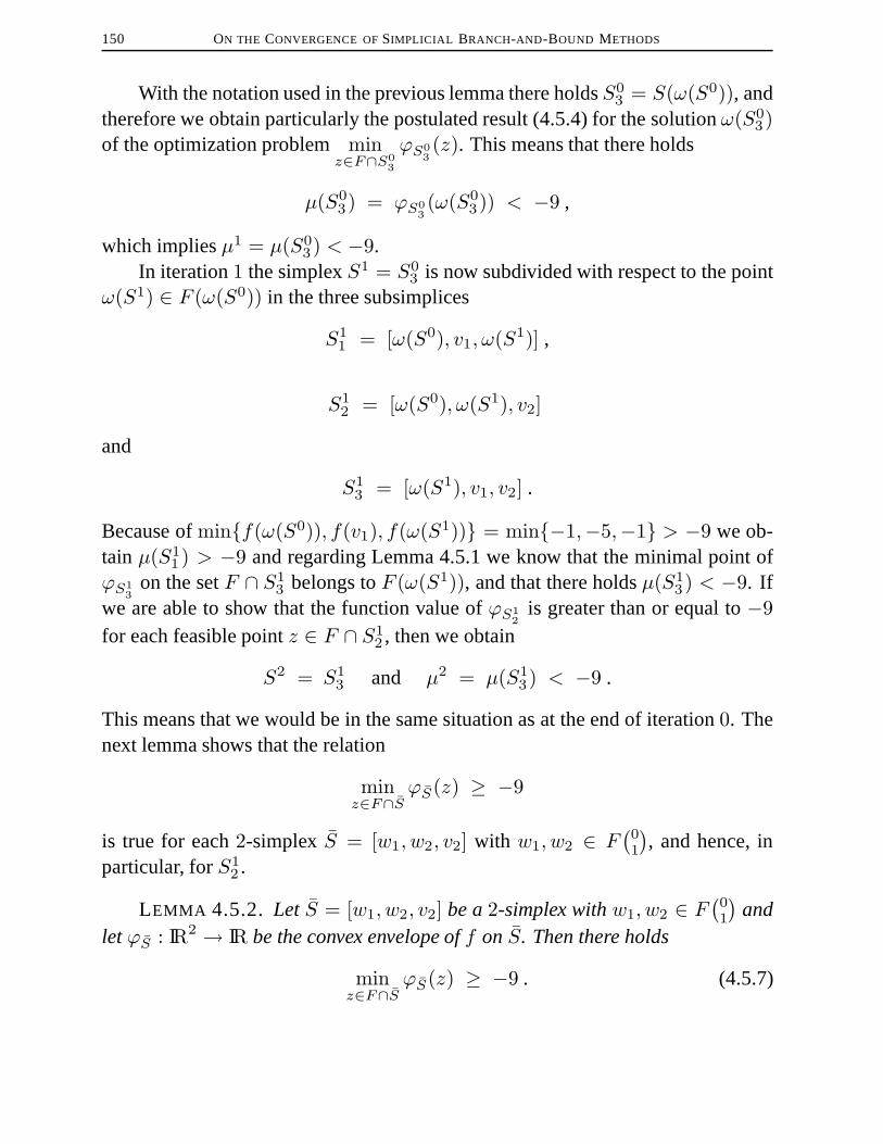
150 ON THE CONVERGENCE OFSIMPLICIAL BRANCH-AND-BOUND METHODS
With the notation used in the previous lemma there holdsS03 = S(ω(S0)), and
therefore we obtain particularly the postulated result (4.5.4) for the solutionω(S03)
of the optimization problem minz∈F∩S0
3
ϕS03(z). This means that there holds
µ(S03) = ϕS0
3(ω(S0
3)) < −9 ,
which impliesµ1 = µ(S03) < −9.
In iteration1 the simplexS1 = S03 is now subdivided with respect to the point
ω(S1) ∈ F (ω(S0)) in the three subsimplices
S11 = [ω(S0), v1, ω(S1)] ,
S12 = [ω(S0), ω(S1), v2]
and
S13 = [ω(S1), v1, v2] .
Because ofmin{f(ω(S0)), f(v1), f(ω(S1))} = min{−1,−5,−1} > −9 we ob-tain µ(S1
1 ) > −9 and regarding Lemma 4.5.1 we know that the minimal point ofϕS1
3on the setF ∩ S1
3 belongs toF (ω(S1)), and that there holdsµ(S13) < −9. If
we are able to show that the function value ofϕS12
is greater than or equal to−9for each feasible pointz ∈ F ∩ S1
2 , then we obtain
S2 = S13 and µ2 = µ(S1
3) < −9 .
This means that we would be in the same situation as at the end of iteration0. Thenext lemma shows that the relation
minz∈F∩S
ϕS(z) ≥ −9
is true for each2-simplex S = [w1, w2, v2] with w1, w2 ∈ F(01
), and hence, in
particular, forS12 .
LEMMA 4.5.2. Let S = [w1, w2, v2] be a2-simplex withw1, w2 ∈ F(01
)and
letϕS : IR2 → IR be the convex envelope off on S. Then there holds
minz∈F∩S
ϕS(z) ≥ −9 . (4.5.7)

4.5. A COUNTEREXAMPLE 151
FIGURE 4.4. Situation in Lemma 4.5.2
������������������
������������������
w2
w1
w2
C
w1v2S \ C
PROOF: There holdsϕS(w1) = ϕS(w2) = −1 andϕS(v2) = −17. Withwi := 0.5wi + 0.5v2 (i = 1, 2) we obtain, fori = 1, 2,
ϕS(wi) = −9 ,
and hence
ϕS(z) ≥ −9 ∀z ∈ [w1, w2, w1, w2] =: C .
In order to show result (4.5.7) it is sufficient to prove that each element ofS \C isinfeasible with respect to Problem (CE) (see Figure 4.4).
Letw be an arbitrary element ofS \ C, i.e.,
w =(wx
wy
) ∈ [v2, w1, w2] .
By definition of wi (i = 1, 2) we obtainwx ≤ −0.5 andwy ≥ 2.0. It followsimmediately1
4w2x + w2
y > 1, i.e.,w /∈ F . �
Combining the results of Lemma 4.5.1 and Lemma 4.5.2 and regarding theconsiderations above we see that the variant of Algorithm 4.1, which uses onlyω-subdivisions, generates an infinite sequence{Sk}k∈INof simplices with the prop-erties that, for eachk ∈ IN, there holds
Sk = [ω(Sk−1), v1, v2] ,
ω(Sk) ∈ F (ω(Sk−1))and
µk = µ(Sk) < −9 .
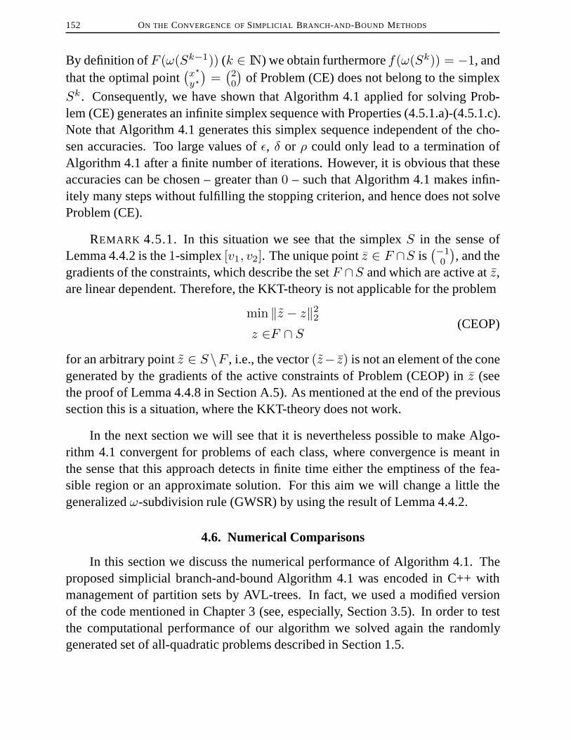
152 ON THE CONVERGENCE OFSIMPLICIAL BRANCH-AND-BOUND METHODS
By definition ofF (ω(Sk−1)) (k ∈ IN) we obtain furthermoref(ω(Sk)) = −1, andthat the optimal point
(x?
y?
)=(20
)of Problem (CE) does not belong to the simplex
Sk. Consequently, we have shown that Algorithm 4.1 applied for solving Prob-lem (CE) generates an infinite simplex sequence with Properties (4.5.1.a)-(4.5.1.c).Note that Algorithm 4.1 generates this simplex sequence independent of the cho-sen accuracies. Too large values ofε, δ or ρ could only lead to a termination ofAlgorithm 4.1 after a finite number of iterations. However, it is obvious that theseaccuracies can be chosen – greater than0 – such that Algorithm 4.1 makes infin-itely many steps without fulfilling the stopping criterion, and hence does not solveProblem (CE).
REMARK 4.5.1. In this situation we see that the simplexS in the sense ofLemma 4.4.2 is the1-simplex[v1, v2]. The unique pointz ∈ F ∩S is
(−10
), and the
gradients of the constraints, which describe the setF ∩S and which are active atz,are linear dependent. Therefore, the KKT-theory is not applicable for the problem
min ‖z − z‖22z ∈F ∩ S (CEOP)
for an arbitrary pointz ∈ S \F , i.e., the vector(z− z) is not an element of the conegenerated by the gradients of the active constraints of Problem (CEOP) inz (seethe proof of Lemma 4.4.8 in Section A.5). As mentioned at the end of the previoussection this is a situation, where the KKT-theory does not work.
In the next section we will see that it is nevertheless possible to make Algo-rithm 4.1 convergent for problems of each class, where convergence is meant inthe sense that this approach detects in finite time either the emptiness of the fea-sible region or an approximate solution. For this aim we will change a little thegeneralizedω-subdivision rule (GWSR) by using the result of Lemma 4.4.2.
4.6. Numerical Comparisons
In this section we discuss the numerical performance of Algorithm 4.1. Theproposed simplicial branch-and-bound Algorithm 4.1 was encoded in C++ withmanagement of partition sets by AVL-trees. In fact, we used a modified versionof the code mentioned in Chapter 3 (see, especially, Section 3.5). In order to testthe computational performance of our algorithm we solved again the randomlygenerated set of all-quadratic problems described in Section 1.5.

4.6. NUMERICAL COMPARISONS 153
We are interested in (ε, δ, ρ)-solutions of Problem (DCP) withε, δ, ρ > 0. Notethat the test examples were generated in a way, which ensured that the feasible setF is not empty. In view of the Convergence Theorem 4.3.1 we know that the variantof Algorithm 4.1, which employs only bisections, detects such a solution in finitetime. Using the generalizedω-subdivision rule (GWSR) the finiteness of Algorithm4.1 is no longer guaranteed, at least in the general case. Nevertheless, it is possibleto make this variant of Algorithm 4.1 finite, as we will see later in this section. Forthis purpose we will modify (GWSR) by using the result of Lemma 4.4.2.
4.6.1. Comparison of Algorithm 4.1 Based on Bisection with Algorithm3.1. First of all we would like to compare the computational performances of Al-gorithm 4.1 employing bisections and of Algorithm 3.1 (see Section 3.3). The usedsubproblems are the main difference between Algorithm 3.1 and Algorithm 4.1, ifwe apply these approaches for solving all-quadratic problems (QP). Note that wealso use a (δ, ρ)-feasibility concept in order to obtain finiteness of Algorithm 3.1(see the considerations at the end of Section 3.4). In Algorithm 3.1 we obtain lowerbounds by linearizing the original Problem (QP) with respect to the current simplex(see Section 3.2) and in Algorithm 4.1 we use convex subproblems. Since the con-vex relaxation of an all-quadratic problem, presented in Section 4.2 for Algorithm4.1, is of course a better approximation than the linear relaxation proposed in Sec-tion 3.2 for Algorithm 3.1 (see also Remark 3.2.1), we can expect that Algorithm4.1 needs less iterations than Algorithm 3.1 in order to solve this problem. Howmuch the running-times change is not predictable in advance. They can decrease,but also increase.
We solved all test problems with Algorithm 3.1 using the LP-subroutineE04NFFof theNAG-library. Since there is no sparse structure in our linear sub-problems it is not reasonable to useMINOS 5.4, as we did in Section 3.5. Note thatthis tool is slower than E04NFF, if both are applied for solving non-sparse prob-lems (compare with the computational results in Section 3.5 and the reason there touseMINOS 5.4). As aCONVEXSOLVERε,δ,ρ in Algorithm 4.1 we used theNAG-subroutineE04UCCwith the default value ofε depending on the machine precisionandδ = ρ = 10−6. This routine implements asequential quadratic programming(SQP) method. In both algorithms we used the accuraciesε = δ = 10−4 andρ = 10−6. As in the numerical tests in Section 3.5 we stopped branching in bothalgorithms, when therelativedifference betweenηk andµk (k ∈ IN) was smaller

154 ON THE CONVERGENCE OFSIMPLICIAL BRANCH-AND-BOUND METHODS
than the toleranceε, i.e., if there held
ηk − µk ≤ ε max{1.0 , |ηk|} (SC)
(compare with page 103).
REMARK 4.6.1. We do not solve Problem (DCPS) directly with theCON-VEXSOLVERε,δ,ρ . In order to avoid the calculation of the vectorsvSi (see (4.2.3.a)and (4.2.3.b)) (i = 0, . . . , n) it is cheaper to affinely transform Problem (DCPS) byusingx = v0 +WSλ, whereWS denotes the regular (n× n)-matrix with columns(vi − v0) (i = 1, . . . , n) andλ is an element of{λ ∈ IRn :
∑ni=1 λi ≤ 1 , λ ≥ 0}.
By doing this we do not need the constraints(vSi )Tx ≤ cSi in order to ensurethat the feasible points of Problem (DCPS) are contained in the current simplexS = [v0, . . . , vn]. It is sufficient to require that there holdsλ ∈ [0, 1]n and∑n
i=1 λi ≤ 1 (see the derivation of the LP-relaxation in Section 3.2 and, espe-cially, the Remarks 3.2.1 and 3.2.2(a)).
Tables 4.1 and 4.2 show some numerical results for the generated test prob-lems run on aSUN SPARCserver 1000workstation. We use the abbreviations NuPCo<Li for the number of problems where Algorithm 4.1 with convex subproblemswas faster with respect to the running-time than Algorithm 3.1 with linear subprob-lems. AvgNuSP is used for the average number of subproblems solved for eachtest problem with Algorithm 4.1 (Co) or Algorithm 3.1 (Li). StdSP is used for thestandard deviation of the number of subproblems. AvgTime stands for the aver-age computing time in seconds necessary for solving a problem and StdTime forthe corresponding standard deviation values. Note that in the numerical tests ofAlgorithm 3.1 in Section 3.5 we used higher accuracies for checking the"feasibil-ity" of generated solutionsω(Sk). Therefore, Algorithm 3.1 had in the numericaltests in the present chapter on average less linear subproblems to solve than it wasthe case in Section 3.5 (see Tables 3.1 and 3.2). The results for Algorithm 3.1were obtained with the original variant of this approach, which did not apply anyselection rule for the first vertex of a consideredn-simplex (see Subsection 3.5.3).
The numerical results displayed in Table 4.1 show that for small dimensionalproblems (n ≤ 4) the decrease of the number of subproblems, which had to besolved, did not lead to a decrease of the running-time. Algorithm 4.1 with convexsubproblems needed on average the same or slightly more time in order to solve thetest problems than the other one did. However, as we can see in Table 4.2, if morethan twice as much linear subproblems had to be solved, Algorithm 4.1 showed a

4.6. NUMERICAL COMPARISONS 155
TABLE 4.1. All test results forn = 2, 3, 4
p NuP AvgNuSP StdSP AvgTime StdTimeCo<Li Co Li Co Li Co Li Co Li
n = 2
1 21 29.6 42.0 12.9 17.1 0.12 0.11 0.05 0.042 20 23.6 38.2 12.4 18.8 0.12 0.13 0.06 0.083 12 33.9 55.5 14.1 30.4 0.19 0.16 0.09 0.074 3 34.4 50.2 11.1 23.4 0.21 0.14 0.08 0.06n = 3
1 16 78.4 122.5 52.2 83.0 0.43 0.42 0.29 0.302 14 80.2 133.0 47.1 131.7 0.47 0.44 0.32 0.383 9 101.4 173.0 67.6 145.1 0.68 0.55 0.45 0.434 6 82.0 132.0 43.4 74.7 0.57 0.42 0.28 0.225 8 88.3 156.4 48.4 106.8 0.74 0.53 0.44 0.336 10 88.8 159.5 44.5 86.2 0.70 0.56 0.33 0.33n = 4
1 14 172.6 304.4 145.8 316.4 1.27 1.12 1.07 1.102 14 179.2 324.4 158.4 323.9 1.39 1.35 1.26 1.383 10 155.3 310.2 105.9 372.1 1.28 1.26 0.86 1.434 18 234.1 536.2 214.7 741.2 2.14 2.24 2.17 3.135 10 178.4 332.6 110.7 257.7 1.67 1.41 1.12 1.036 10 228.5 671.6 202.5 1,661 2.32 3.47 2.12 10.107 10 207.2 382.3 141.6 292.9 2.22 1.82 1.53 1.348 4 204.6 372.9 154.1 378.2 2.43 1.92 1.85 1.98
better numerical performance with respect to the running-time than Algorithm 3.1.With growing dimensions and, in particular, with a growing number of quadraticconstraints the relative difference between the average number of convex subprob-lems and the average number of linear subproblems increased. For dimensionshigher thann = 6 Algorithm 4.1 solves more than60% of the 50 test problemsfaster than Algorithm 3.1. On average Algorithm 4.1 was always faster for thesetest problems. Since the speedup, i.e., the quotient of the average running-timewith linear subproblems and the average running-time with convex subproblemswas mostly less than1.5, we see that the use of convex subproblems was not a sub-stantial acceleration of the considered solution process for all-quadratic problems.However, there was a small acceleration.
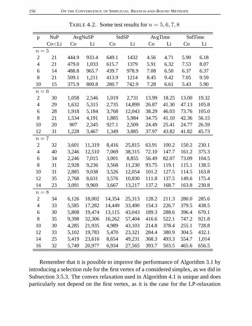
156 ON THE CONVERGENCE OFSIMPLICIAL BRANCH-AND-BOUND METHODS
TABLE 4.2. Some test results forn = 5, 6, 7, 8
p NuP AvgNuSP StdSP AvgTime StdTimeCo<Li Co Li Co Li Co Li Co Li
n = 5
2 21 444.9 933.4 649.1 1432 4.56 4.71 5.90 6.184 21 479.0 1,033 615.7 1379 5.91 6.32 7.53 8.076 14 488.8 965.7 439.7 978.9 7.08 6.50 6.37 6.378 21 509.1 1,211 413.9 1214 8.45 9.42 7.05 9.5910 15 375.9 800.8 280.7 742.9 7.28 6.61 5.43 5.90n = 6
2 30 1,058 2,546 1,019 2,731 13.99 18.25 13.00 19.324 29 1,632 5,315 2,735 14,899 26.87 41.30 47.13 105.86 28 1,918 5,184 3,768 12,043 38.29 46.03 73.76 105.08 21 1,534 4,191 1,885 5,984 34.75 41.10 42.36 56.1510 20 907 2,345 927.1 2,509 24.49 25.41 24.77 26.5912 31 1,228 3,467 1,349 3,885 37.97 43.82 41.82 45.73n = 7
2 32 3,601 11,319 8,416 25,815 63.91 100.2 150.2 230.14 40 3,246 12,510 7,069 38,315 72.10 147.7 161.2 375.36 34 2,246 7,015 3,001 8,855 56.49 82.07 73.09 104.58 31 2,928 9,236 3,568 11,230 93.75 119.1 115.1 138.510 31 2,885 9,038 3,526 12,054 101.2 127.5 114.5 163.812 35 2,768 8,631 3,576 10,830 111.8 137.5 149.6 175.414 23 3,091 9,969 3,667 13,217 137.2 168.7 163.8 230.8n = 8
2 34 6,126 18,002 14,354 25,313 128.2 211.3 280.0 285.64 33 5,585 17,282 14,449 33,490 154.3 226.7 379.5 438.56 30 5,808 19,474 13,115 43,043 189.3 288.6 396.4 670.18 35 9,398 32,306 16,262 57,404 416.6 522.1 747.2 921.810 30 4,285 21,935 4,989 43,103 214.8 378.4 255.1 728.812 33 5,102 19,783 5,470 23,321 284.4 380.9 304.5 432.114 25 5,419 23,616 8,654 49,231 368.3 493.3 554.7 1,01416 32 5,749 20,977 6,934 27,565 393.7 503.5 465.6 656.5
Remember that it is possible to improve the performance of Algorithm 3.1 byintroducing a selection rule for the first vertex of a considered simplex, as we did inSubsection 3.5.3. The convex relaxation used in Algorithm 4.1 is unique and doesparticularly not depend on the first vertex, as it is the case for the LP-relaxation

4.6. NUMERICAL COMPARISONS 157
applied in Algorithm 3.1. Hence such a selection rule does not alter the numer-ical performance of Algorithm 4.1 and, in view of the results in Table 3.4, it islikely that the use of a selection rule in Algorithm 3.1 reduces the running-timeadvantage of Algorithm 4.1. On the other hand, in Algorithm 4.1 we applied aCONVEXSOLVERε,δ,ρ , which only uses the differentiability of the convex func-tions. Maybe another solution method, which exploits the quadratic structure of(DCPS), can solve the occurring convex subproblems faster (see, e.g., [JAR96]).Thus, we can expect that Algorithm 4.1 with convex subproblems is – with respectto the running-time – a better solution method for all-quadratic optimization prob-lems than Algorithm 3.1 with linear subproblems, at least for dimensions higherthann = 4.
Another interesting numerical effect of the use of convex subproblems insteadof linear subproblems is that the standard deviation values are in some cases sig-nificantly smaller. Note that, especially in Table 4.2, for the numbers of solvedsubproblems as well as for the running-times the values of the standard deviationare very high, when they are compared with the average values. The reason is that,in particular for growing dimensions, the number of test problems, which neededsubstantially more time to be solved than the average, increased, and that the dif-ference between the effort for solving such numerical outliers and the effort forsolving average problems also grew. These effects were stronger if linear subprob-lems were used. From this point of view we see that Algorithm 4.1 shows, at least
TABLE 4.3. Comparison of the medians of the running-times ofAlgorithm 4.1 based on bisection and of Algorithm 3.1
p = 2 p = 4 p = 6 p = 8 p = 10 p = 12 p = 14 p = 16
n = 5
Co 2.64 3.53 5.14 6.06 6.06Li 2.93 3.83 4.75 4.99 4.96
n = 6
Co 10.21 14.39 15.97 21.04 16.51 23.84Li 14.18 15.12 16.01 19.70 17.04 30.03
n = 7
Co 27.08 35.69 29.15 55.18 70.46 71.66 78.11Li 34.20 47.23 35.97 73.75 64.33 88.12 72.13
n = 8
Co 34.61 59.79 68.14 136.4 114.4 179.8 192.0 191.1Li 52.63 98.18 92.30 204.9 133.5 215.9 174.3 234.7

158 ON THE CONVERGENCE OFSIMPLICIAL BRANCH-AND-BOUND METHODS
for the examined test problems, a more stable behavior in the sense that less nu-merical outliers occur. In view of the existence of numerical outliers we can expectthat a large number of test problems could be solved with less effort than the av-erage values imply. In Table 4.3 we display the medians of the running-times inseconds, corresponding to the numerical results of Table 4.2. The presented valuesshow that at least50% of the test problems could be solved significantly faster thanthe average. We also see that the medians of the running-times for Algorithm 4.1(Co) are not always smaller than the corresponding values for Algorithm 3.1 (Li),as it is the case for the average values, at least for dimensions higher thann = 5(see Table 4.2). This corroborates the effect mentioned above that the use of convexsubproblems reduces the occurrence of numerical outliers and the worst case effort,respectively.
4.6.2. A Convergent Subdivision Rule Based on (GWSR).In the followingwe would like to use Algorithm 4.1 with the (GWSR) strategy in order to solve thesame set of test problems. Since – in view of Section 4.5 – we cannot be sure thatthe variant of Algorithm 4.1, which employs only the generalizedω-subdivisionrule, detects in finite time an (ε, δ, ρ)-solution, we introduce a modification of(GWSR) ensuring finiteness of Algorithm 4.1.
For this aim we will exploit the result of Lemma 4.4.2. At the end of Section4.4 we pointed out that also in the general case (DCP3) all results until Lemma4.4.7 are provable for Algorithm 4.1 using aCONVEXSOLVERεk,δk,0 (k ∈ IN).As long as a solution method for the convex subproblems is used, which generatesa pointω(Sk) ∈ Sk, we know thatwk is chosen asω(Sk) in the (GWSR)-rule(if δk ≤ δ and εk ≤ ε, see Remark 4.2.2(h)). In the numerical tests we use aCONVEXSOLVERε,δ,ρ with arbitrary accuraciesε, δ, ρ > 0. Therefore, there doesnot necessarily holdω(Sk) ∈ Sk, and it is not immediately clear that at leastthe results of Lemma 4.4.2 still hold. Nevertheless, if the accuraciesε, δ andρ arechosen as in the following lemma, then we are able to prove all results until Lemma4.4.2 for the version of Algorithm 4.1 with (GWSR) also in the general case.
LEMMA 4.6.1. Let ε, δ, ρ ≥ 0 be given. LetLl be a Lipschitz constant ofgl
(l ∈ {0, . . . , p}) on then-simplex
S0 = {x ∈ IRn : (vS0
i )Tx ≤ cS0
i + ρ , i = 0, . . . , n}(see (4.2.2) for the definition ofvS
0
i andcS0
i ), letD ∈ IRn be an upper bound for‖ · ‖2 onS0 = [v0
0 , . . . , v0n], e.g.,D = maxi=0,... ,n ‖v0
i ‖2, and letCl be an upper

4.6. NUMERICAL COMPARISONS 159
bound forf l (l ∈ {0, . . . , p}) on the same set. Fork ∈ IN denote by
Ik := {i ∈ {0, . . . , n} : λki > 0}with λk ∈ {λ ∈ IRn+1 :
∑ni=0 λi = 1}, ω(Sk) =
∑ni=0 λ
ki vki and set
wk :=∑i∈Ik
λkiγkvki
with γk =∑
i∈Ik λki . If ω(Sk) is an (ε, δ, ρ)-solution of (DCPSk
) with
ε ≤ 14ε , δ ≤ 1
4δ
and
ρ ≤ min{ρ
4,
ρ
4nD‖ai‖2 , i = 1, . . . ,m ,δ
4n(Cl +DLl), l = 1, . . . , p ,
ε
4n(C0 +DL0)
},
then there holds
wk is a (34δ,34ρ)-feasible point for (DCPS
k
) (4.6.1.a)
and
g0(wk) + ϕ0Sk(wk) ≤ µ(Sk) + 3
4ε . (4.6.1.b)
PROOF: In the proof of Theorem 4.3.1 we showed that, ifω(Sk) is an(ε, δ, ρ)-solution of (DCPS
k
), then there holds, for eachk ∈ IN andi ∈ {0, . . . , n},λki ≥ −ρ .
Therefore, using the relation∑i∈Ik
(λki −
λkiγk
)= γk − 1 =
∑i/∈Ik
|λki |
we obtain∑i∈Ik
(λki −
λkiγk
)+∑i/∈Ik
|λki | = 2∑i/∈Ik
|λki |︸︷︷︸≤ρ
≤ 2nρ . (4.6.2)|Ik| ≥ 1
Because of the definition ofwk it follows
‖ω(Sk)− wk‖2 = ‖∑i∈Ik
(λki −
λkiγk
)vki +
∑i/∈Ik
λki vki ‖2

160 ON THE CONVERGENCE OFSIMPLICIAL BRANCH-AND-BOUND METHODS
≤ D
∑i∈Ik
(λki −
λkiγk
)+∑i/∈Ik
|λki | ≤ 2nDρ (4.6.3)
(4.6.2)
and, forl ∈ {0, . . . , p},
|ϕlSk(ω(Sk))− ϕlSk(wk)| = |∑i∈Ik
(λki −
λkiγk
)f l(vki ) +
∑i/∈Ik
λki fl(vki )|
≤ Cl
∑i∈Ik
(λki −
λkiγk
)+∑i/∈Ik
|λki | ≤ 2nClρ . (4.6.4)
(4.6.2)
From (4.6.3) and (4.6.4) we conclude, fori ∈ {1, . . . ,m},aTi w
k ≤ aTi ω(Sk)︸ ︷︷ ︸≤bi+ρ
+ |aTi wk − aTi ω(Sk)|︸ ︷︷ ︸≤‖ai‖2‖wk−ω(Sk)‖2
≤ bi + ρ︸︷︷︸≤ ρ
4
+ ‖ai‖22nDρ︸ ︷︷ ︸≤ ρ
2
≤ bi + 34ρ (4.6.5)
and, forl ∈ {1, . . . , p},gl(wk) + ϕlSk(wk) ≤ gl(ω(Sk)) + ϕlSk(ω(Sk)) + |gl(ω(Sk))− gl(wk)|︸ ︷︷ ︸
≤Ll‖ω(Sk)−wk‖2
+ |ϕlSk(ω(Sk))− ϕlSk(wk)|︸ ︷︷ ︸≤2nClρ
≤ δ + 2nDLlρ+ 2nClρ
≤ δ︸︷︷︸≤ δ
4
+ 2n(DLl + Cl)ρ︸ ︷︷ ︸≤ δ
2
≤ 34δ , (4.6.6)
which shows the (34δ,34ρ)-feasibility of wk with respect to the feasibility set of
(DCPSk
). In order to show (4.6.1.b) we obtain by the same argumentation as in(4.6.6)
g0(wk) + ϕ0Sk(wk) ≤ g0(ω(Sk)) + ϕ0
Sk(ω(Sk))︸ ︷︷ ︸≤µ(Sk)+ε
+ 2n(DL0 + C0)ρ︸ ︷︷ ︸≤ ε
2
≤ µ(Sk) + 34ε .
�

4.6. NUMERICAL COMPARISONS 161
REMARK 4.6.2.
(a) It follows immediately that the situation|Ik| = 1 (see (GWSR)) cannotoccur, if ε, δ andρ are chosen as in the previous lemma. Indeed,|Ik| = 1means that
wk =∑i∈Ik
λkiγkvki ∈ {vk0 , . . . , vkn} .
Regarding (4.6.1.a) and because ofϕlSk(vki ) = f l(vki ) (i ∈ {0, . . . , n}),we know that there is a (δ, ρ)-feasible vertexvki′ ∈ {vk0 , . . . , vkn}. Sinceeach vertex ofSk (k ∈ IN) is used for updating the upper bound in previousiterations of Algorithm 4.1 and in view of (4.6.1.b), there holds
ηk ≤ g0(vki′ ) + f0(vki′ ) = g0(wk) + ϕ0Sk(wk)
≤ µ(Sk)︸ ︷︷ ︸<ηk−ε
+ 34ε < ηk − 1
4ε ,
which is a contradiction.(b) In the quadratic case the Lipschitz constantsLl (l ∈ {0, . . . , p}) can be
calculated in the following way
Ll = maxx∈V (S0)
‖∇f l(x)‖2 ,
whereV (S0) denotes the vertex set ofS0. For the calculation ofLl in thegeneral case we refer to Section B.2.
(c) Since we have aCONVEXSOLVERε,δ,ρ for arbitrary accuraciesε, δ, ρ > 0the necessary upper boundsCl for the concave functionsf l (l ∈ {0, . . . , p})on the setS0 can be determined using this solution method.
With the result of Lemma 4.6.1 and using an analogous argumentation as inthe proof of Lemma 4.4.1 the following corollary is easy to verify.
COROLLARY 4.6.2. Assume thatε, δ, ρ > 0. LetSk be the selected simplexin iteration k ∈ IN of Algorithm 4.1 employing the generalizedω-subdivision rule(GWSR), letω(Sk) be an (ε, δ, ρ)-solution of (DCPS
k
) with ε, δ and ρ chosen asin Lemma 4.6.1, and letS? be one of the simplices obtained by subdividingSk
with respect towk. If Sk is not fathomed in the pruning rule (PR) of Algorithm4.1, then there holds, for eachx ∈ S? with x =
∑nj=0,j 6=i λjv
kj + λiw
k, λ ∈ Bn,

162 ON THE CONVERGENCE OFSIMPLICIAL BRANCH-AND-BOUND METHODS
i ∈ {0, . . . , n},ϕ0S?(x) ≥ ϕ0
Sk(x) + 14ελi , if wk is (δ, ρ)- feasible,
or∃l ∈ {1, . . . , p} : ϕlS?(x) ≥ ϕlSk(x) + 1
4δλi , otherwise.
(4.6.7)
PROOF: As mentioned above, this proof is analogous to the proof of Lemma4.4.1. Therefore, we would not like to expatiate this proof. However, note that –regarding Remark 4.6.2(a) – there holds
wk =∑i∈Ik
λkiγkvki /∈ {vk0 , . . . , vkn} ,
i.e, |Ik| > 1 in (GWSR). Note, furthermore, thatwk is, in view of Lemma 4.6.1,alwaysρ-feasible with respect to the linear constraints of (DCP). �
The result of this corollary coincides with Lemma 4.4.1, where this lemma wasthe essential part in the proof of Lemma 4.4.2. A careful checking of the proofs forLemma 4.4.2 (see Appendix A, especially the proof of Lemma A.1) shows that thisresult is also true in the general case of problems of type (DCP3), if the assumptionsof Corollary 4.6.2 are fulfilled.
COROLLARY 4.6.3. Assume thatε, δ andρ are chosen greater than0 in theinitialization of Algorithm 4.1, and assume that aCONVEXSOLVERε,δ,ρ is usedwith ε, δ and ρ chosen as in Lemma 4.6.1. Let{Sk}k∈IN be an infinite nestedsequence of simplices generated by the variant of Algorithm 4.1, which employsonly (GWSR). Assume further that this sequence has the properties that, for eachk ∈ IN, there holds
Sk+1 = [vk0 , . . . , vki−1, w
k, vki+1, . . . , vkn]
andµ(Sk) < ηk − ε .
Then there exist a numberK ∈ IN and an integerr with 0 ≤ r < n, such that
Sk = [v0, . . . , vr, vkr+1, . . . , vkn] ∀k ≥ K ,
wherev0, . . . , vr are fixed vectors, whilevkr+1, . . . , vkn (k ∈ IN, k ≥ K) change
infinitely often. Moreover, there holds⋂k∈S
Sk = [v0, . . . , vr] =: S .

4.6. NUMERICAL COMPARISONS 163
If we modify the generalizedω-subdivision rule in such a way, that in theresult of Corollary 4.6.3 there must holdr = 0, then we can obtain an algorithm,which delivers in finite time either an (ε, δ, ρ)-solution of Problem (DCP) withε, δ,ρ > 0 or the emptiness ofF . The followingmodified generalizedω-subdivisionrule (MGWSR) yields this intention. For this rule we need an additional counterN(i, Sk), which shows how long the vertexvki (i ∈ {0, . . . , n}) of Sk did notchange.
In the initialization phase of Algorithm 4.1 we set, for eachi ∈ {0, . . . , n},N(i, S0) = 0, and in each iteration this counter is adjusted, for each simplexSkj(j ∈ Ik), in the following way
N(i, Skj ) = N(i, Sk) + 1 , if i ∈ {0, . . . , n} \ {j}N(j, Skj ) = 0 .
In order to formulate the modified rule we need, additionally, an arbitrary, but fixednumberN ∈ IN, which has to be chosen in the initialization phase of Algorithm4.1. The (MGWSR) is now as follows.
Chooseλk ∈ {λ ∈ IRn+1 :∑n
i=0 λi = 1} with ω(Sk) =∑ni=0 λ
ki vki .
Ik ← {i ∈ {0, . . . , n} : λki > 0}If |Ik| = 1 Thenwk ← 1
2
(vki0 + vki1
)(SR1)
(i.e., choose a classical bisection, see (4.2.12) for the definition ofi0 andi1)
ElseDetermineN1 andi2 with N1 = N(i2, Sk) = maxi∈{0,... ,n}N(i, Sk)andN2 = maxi∈{0,... ,n}\{i2}N(i, Sk).If N2 > N Thenwk ← 1
2
(vki0 + vki1
)(SR2)
ElseDetermineγk :=
∑i∈Ik λki
wk ← ∑i∈Ik
λki
γk vki (SR3)
EndIfEndIf

164 ON THE CONVERGENCE OFSIMPLICIAL BRANCH-AND-BOUND METHODS
THEOREM 4.6.4. Assume thatε, δ and ρ are chosen greater than0 in theinitialization of Algorithm 4.1, and assume that aCONVEXSOLVERε,δ,ρ is usedwith ε, δ andρ chosen as in Lemma 4.6.1. Then the variant of Algorithm 4.1, whichemploys only (MGWSR), detects for Problem (DCP), in particular for (DCP3), infinite time either the emptiness of the feasible regionF or an (ε, δ, ρ)-solution.
PROOF: Assume, by contradiction, that Algorithm 4.1 is not finite and let, withoutloss of generality,{Sk}k∈IN be an infinite nested sequence of simplices generatedby this approach with the propertyµ(Sk) < ηk − ε (k ∈ IN). In view of Remark4.6.2(a) we know thatwk must be chosen by the selection rules (SR2) or (SR3). Ifthere holds
|{k ∈ IN : wk is chosen by (SR2)}| < ∞ , (4.6.8)
then we can assume thatwk (k ∈ IN) is always chosen by (SR3). With respectto Corollary 4.6.3 we obtain the existence of a numberK ∈ IN and an integer0 ≤ r < n with
Sk = [v0, . . . , vr, vkr+1, . . . , vkn] ∀k ≥ K .
Since eachwk is chosen by (SR3) there holdsr = 0. Otherwise, we would obtain
min {N(0, Sk) , N(1, Sk)} > N
for k ∈ IN big enough, which would force the selection ofwk by (SR2). The factthat r is equal to0 together with the second result of Corollary 4.6.3 implies theexhaustiveness of the sequence{Sk}k∈IN, and, because ofε, δ, ρ > 0, Theorem4.3.1 yields a contradiction.
Therefore, (4.6.8) cannot be true, i.e., an infinite number of elements of{Sk}k∈IN must be generated by the classical bisection rule. Denote byd(Sk) :=maxi,j=0,... ,n ‖vki −vkj ‖2 the diameter ofSk and the maximal distance ofwk to anyvertex ofSk by d(wk, Sk) := maxi=0,... ,n ‖wk − vki ‖2. If there exists a constantvalueτ ∈ (0, 1) with the property that, for eachk ∈ IN, there holds
d(wk, Sk) ≤ τd(Sk) , (4.6.9)
then it is a known fact [HT96B, Proposition VII.4] that infinitely many bisectionsguarantee the exhaustiveness of{Sk}k∈IN.
As mentioned before we know, in view of Theorem 4.3.1 and because ofε, δ,ρ > 0, that{Sk}k∈IN cannot shrink to a singleton. Thus, there does not exist a value
4.6. NUMERICAL COMPARISONS 165
τ ∈ (0, 1) with property (4.6.9). I.e., there is at least a subsequence{Skq}q∈IN of{Sk}k∈IN with
d(wkq , Skq)d(Skq )
→ 1 (q →∞) (4.6.10)
and, for eachq ∈ IN,
wkq is chosen by (SR3) .
Note that{d(Sk)}k∈IN is a non-increasing sequence, which is, in view of the non-exhaustiveness of{Sk}k∈IN, convergent to a real valued > 0, and note, further-more, that there holds
d(wk, Sk) ≤√
32 d(S
k) ,
if wk is chosen by bisection (see, e.g., the proof of Proposition 3.14 in [HPT95]).Since each vertex sequence{vkq
i }q∈IN (i ∈ {0, . . . , n}) is bounded, we can as-sume, without loss of generality, that they are convergent to pointsvi(i = 0, . . . , n). Letλq ∈ Bn (q ∈ IN) be chosen such that
wkq =n∑i=0
λqi vkq
i .
Because of the boundedness of{λq}q∈IN we can further assume, without loss ofgenerality, that this sequence is also convergent to a vectorλ ∈ Bn and we obtain
wkq →n∑i=0
λivi =: w . (4.6.11)
We prove now that, taking (4.6.10) into account, there holds
w ∈ {v0, . . . , vn} . (4.6.12)
PROOF OF(4.6.12): Obviously we know that
d(Skq ) → maxi,j=0,... ,n
‖vi − vj‖2 = d (q → ∞) . (4.6.13)
For eachq ∈ IN, there is an indexi(q) ∈ {0, . . . , n} with
d(wkq , Skq ) = ‖wkq − vkq
i(q)‖2 .
Assume, without loss of generality, thati(q) is always the same index, i.e.,
d(wkq , Skq ) = ‖wkq − vkq
i′ ‖2 (4.6.14)
for eachq ∈ IN and a fixedi′ ∈ {0, . . . , n}.

166 ON THE CONVERGENCE OFSIMPLICIAL BRANCH-AND-BOUND METHODS
Combining (4.6.10), (4.6.11), (4.6.13) and (4.6.14) we obtain
0 < d = ‖w − vi′‖2 = ‖n∑
j=0
λj vj − vi′‖2
= ‖n∑
j=0
λj (vj − vi′) ‖2 ≤n∑
j=0
λj ‖vj − vi′‖2︸ ︷︷ ︸≤d
≤ d .
Therefore, we see that,
‖n∑
j=0
λj (vj − vi′) ‖2 =n∑
j=0
λj‖ (vj − vi′) ‖2 = d . (4.6.15)
Because ofd > 0 we know that the set
L := {j ∈ {0, . . . , n} : (vj − vi′) 6= 0 andλj > 0}is not empty, and, in view of the right-hand side of (4.6.15), for eachj /∈ L, there holdsλj = 0. Indeed, ifL is empty, then we obtain
∑n
j=0λj‖vj − vi′‖2 = 0 contradicting
d > 0. Moreover, if there is an indexj′ /∈ L with λj′ > 0, then it follows that∑n
j=0λj‖vj − vi′‖2 ≤ ∑n
j=0,j 6=j′ λj d < d contradicting (4.6.15). The left-handequality in Relation (4.6.15) is only possible if there exists, for each pairi, j ∈ L, ascalarγi,j ∈ IR \ {0} with
vi − vi′ = γi,jλj
λi
(vj − vi′) .
Furthermore, again in view of the right-hand equation of (4.6.15), we obtain
‖vi − vi′‖2 = ‖vj − vi′‖2 = d , (4.6.16)
and, therefore,
γi,jλj
λi
∈ {−1, 1} .
Assume thatγi,jλj
λi= −1. Then there holds(vi − vi′) = (vi′ − vj). This implies
2d = ‖2(vi − vi′)‖2 = ‖vi − vi′ + vi′ − vj‖2 = ‖vi − vj‖2 ≤ d ,
which contradictsd > 0. It follows, that there is an indexi′′ ∈ L such that, for eachj ∈ L, there holds
vi′′ = vj ,
and we conclude
w =∑j∈L
λj vj +∑j /∈L
λj︸︷︷︸=0
vj = vi′′∑j∈L
λj︸ ︷︷ ︸=1
= vi′′ ,
i.e., (4.6.12) is true. 2

4.6. NUMERICAL COMPARISONS 167
Assume, without loss of generality, that there holdsw = v0. Since the pointswkq (q ∈ IN) are chosen by (SR3) we know, regarding Lemma 4.6.1, that, foreachq ∈ IN, wkq is (34δ,
34ρ)-feasible for the convex subproblem (DCPSkq
). The
point sequences{wkq}q∈IN and {vkq
0 }q∈IN converge to the same limit pointv0.Therefore, we obtain by continuity off l andgl (l ∈ {0, . . . , p}) (see, e.g., again[ROC70, Theorem 10.1]) and by using the same representation ofwkq (q ∈ IN) asin the proof of (4.6.12), for eachl ∈ {0, . . . , p},
gl(wkq )− gl(vkq
0 ) → 0 (q →∞)and
ϕlSkq (wkq )− f l(vkq
0 ) = ϕlSkq (wkq )− ϕl
Skq (vkq
0 ) → 0 (q →∞) .
It follows, that there exists aQ ∈ IN such that, for eachq ≥ Q,
vkq
0 is (δ, ρ)-feasible
and
g0(vkq
0 ) + f0(vkq
0 ) ≤ g0(wkq ) + ϕ0Skq (wkq ) + 1
8ε . (4.6.17)
Since each (δ, ρ)-feasible vertex of an iteration simplexSk (k ∈ IN) was used forupdating the upper bound, it follows from Relation (4.6.17) and Relation (4.6.1.b)of Lemma 4.6.1 that
g0(vkq
0 ) + f0(vkq
0 ) ≤ µ(Skq) + 78ε < ηkq − 1
8ε ≤ g0(vkq
0 ) + f0(vkq
0 )− 18ε ,
which is also a contradiction and completes the proof. �
4.6.3. Comparison of Different Subdivision Strategies Based on (MGWSR).Theorem 4.6.4 guarantees that Algorithm 4.1 with (MGWSR) delivers in finite timean (ε, δ, ρ)-solution of our test problems, if the accuracies for the usedCONVEX-SOLVERε,δ,ρ are chosen sufficiently small. We implemented the modified gen-eralizedω-subdivision rule and used again theNAG-routineE04UCC, where theaccuraciesε, δ and ρ were calculated as required in Lemma 4.6.1. With this im-plementation we solved all test problems. However, in order to avoid excessiverunning-time we stopped the calculations, if more than200, 000 convex subprob-lems were solved. The variant of Algorithm 4.1, which uses only bisections, neededless than this maximal number of convex subproblems for solving any test problem.The tolerancesε, δ andρ were the same as in the numerical experiments using bi-section and forN we chose2n.

168 ON THE CONVERGENCE OFSIMPLICIAL BRANCH-AND-BOUND METHODS
In Table 4.4 we compare the numerical performance of Algorithm 4.1 using(MGWSR) with the performance of Algorithm 4.1 only employing bisections. Thedisplayed test results for the dimensionsn = 2 andn = 3 were run onSUNSPARC 10workstations. The used abbreviations are the same as in Table 4.1 and4.2. Mω stands for Algorithm 4.1 with (MGWSR) andBi for Algorithm 4.1 usingbisections. Even though Algorithm 4.1 using (MGWSR) was mostly in more than
TABLE 4.4. Comparison of (MGWSR) and bisection
p NuP AvgNuSP StdSP AvgTime StdTimeMω<Bi Mω Bi Mω Bi Mω Bi Mω Bi
n = 2
1 46 16.50 29.64 33.16 12.96 0.13 0.23 0.16 0.102 40 14.94 23.60 26.08 12.40 0.14 0.21 0.17 0.103 43 28.54 33.92 43.50 14.12 0.30 0.34 0.36 0.174 35 86.10 34.40 366.9 10.93 1.31 0.36 3.58 0.13n = 3
1 43 105.6 78.00 386.3 51.47 1.04 0.91 2.97 0.602 37 78.06 80.16 97.05 47.03 1.05 1.03 1.43 0.663 37 181.7 101.3 517.9 67.40 2.76 1.43 6.35 0.954 25 113.1 82.00 131.4 43.38 1.64 1.20 1.64 0.595 30 294.1 88.20 966.1 48.50 3.94 1.40 10.98 0.726 22 205.4 88.80 308.5 44.31 4.52 1.54 7.17 0.72
50% of the test examples faster than Algorithm 4.1 using bisections, the averagerunning-time was only in a few cases lower. Furthermore, the standard deviationof the number of solved convex subproblems as well as of the running-time washigher in the case of (MGWSR) and was growing faster. The reason is that Al-gorithm 4.1 using (MGWSR) was in many test examples slightly faster than theversion of Algorithm 4.1 with bisections, at least for small dimensions, but, in par-ticular for growing dimensions and a growing number of quadratic constraints, thisapproach was in more and more test examples significantly slower than Algorithm4.1 using bisections. For dimensions higher thann = 3 Algorithm 4.1 only em-ploying (MGWSR) did not solve all50 test problems for each couple (n, p) of thedimensionn and the number of quadratic constraintsp with less than200, 000 con-vex subproblems. As it can be seen in Figure 4.5, the number of not-solved testproblems increased with growing dimensions and a growing number of quadraticconstraints. For example, for dimensionn = 8 andp = 16 quadratic constraints

4.6. NUMERICAL COMPARISONS 169
FIGURE 4.5. Number of test problems where Algorithm 4.1 us-ing (MGWSR) needed more than200, 000 convex subproblems
1 2 3 4 5 6 7 8 10 12 14 16
4
5
6
7
8
0
5
10
15
20
25
30
35
40
45
50
Dimension
Number of quadratic constraints
Algorithm 4.1 using (MGWSR) needed less than200, 000 convex subproblems foronly 5 test problems. Remember that the same approach, which used only bisec-tions, solved all test problems with less than this maximal number of calls of thesubroutineE04UCC.
Due to this reason we obtain that Algorithm 4.1 with bisections led to a morerobust solution process, wheremore robustis meant in the following sense. Thenumber of necessary convex subproblems and, thus, the running-time did not varyso keenly, as it was the case, when (MGWSR) was applied. The effort for detectingan (ε, δ, ρ)-solution of the quadratic test problems was rather predictable. Eventhough the variant of Algorithm 4.1, which employs only bisections, was also forhigher dimensions not always the fastest approach, it was a better approach thanthe same algorithm using (MGWSR), since it did not show numerical outliers.
Our numerical experiments further showed a regularization effect of the bisec-tion with respect to the effort for solving the convex subproblems. If the generatedsimplices tend to degenerate, i.e., they become tooflat, as it is possible by using(MGWSR), then numerical problems, e.g., ill-conditioned constraint matrices, can

170 ON THE CONVERGENCE OFSIMPLICIAL BRANCH-AND-BOUND METHODS
occur and can lead to a substantially growing effort for solving the convex subprob-lems. If the classical bisection rule is used, then the risk of the occurrence of suchnumerical problems is much lower. In our numerical tests such problems did notappear in connection with the use of the bisection.
In order to make (MGWSR) more robust in the sense mentioned above, wecould reduce the numberN . With N = 2n Algorithm 4.1 using (MGWSR) chosewk by (SR3) on average in91.5% of the performed subdivisions (see also Table4.8 and Table 4.9). If we reduceN , the number of bisections will increase andthe numerical performance of Algorithm 4.1 using (MGWSR) will approach tothe numerical performance of the variant of this algorithm, which employs onlybisections. Note that, for each nested sequence{Sk}k∈IN, all simplicesSk (k > N )must be generated by bisection, ifN is chosen smaller thann− 1.
As mentioned before, there were also for higher dimensions test exampleswhere the (MGWSR) strategy was the best one. If we simply reduceN , then wewill obtain a more robust algorithm, but, at the end we have nothing else than analgorithm using bisections, and it is likely that we loose the not frequent, but reallygood results of (MGWSR) for some test examples. Maybe it is possible to developa strategy, which is a mixture of the classical bisection rule and (MGWSR), andwhich shows a good performance in all cases, i.e., which use (MGWSR), if thisstrategy is the fastest one, and bisection, if (MGWSR) does not work.
In the case of problems of type (DCP1) we know thatω(Sk) (k ∈ IN) isalways a feasible point, at least if aCONVEXSOLVER0,0,0 is used. Therefore, itis reasonable to hope that this point is a better choice than the point obtained bybisection, sinceω(Sk) is connected to the information returned by the algorithminside the selected simplexSk. This is the main reason for the suggestion of theω-subdivision, e.g., in [HT96B]. In the general case of problems of type (DCP3)the pointω(Sk) is the approximate solution of a subproblem, where the objectivefunction as well as the constraints are relaxed. Therefore, we cannot hope thatω(Sk) has something to do with the solution of the original problem. Ifω(Sk) isat least (δ, ρ)-feasible, then this point is used for updating the upper bound, andwe have more hope thatω(Sk) bears some information about the original problem.Thus the first mixed strategy we used was the following(MGWSR1)

4.6. NUMERICAL COMPARISONS 171
If wk is (δ, ρ)-feasibleThenChoosewk by (MGWSR).
ElseChoosewk by bisection.
EndIf
wherewk is defined as∑
i∈Ikλk
i
γk vki with λk ∈ IRn+1, γk ∈ IR andIk ⊂ {0, . . . , n}
given as in Lemma 4.6.1.This strategy was much more robust than (MGWSR) alone, but the average
running-times for higher dimensions were still slower than by using only bisections.In this case2 test problems withn = 7 and17 problems withn = 8 were notsolved. Therefore, we developed further strategies. In these strategies we try to usemore information about the Problem (DCP).
Denote bymk the middle point of the longest edge ofSk (k ∈ IN), i.e.,
mk = 12 (vki0 + vki1) ,
with i0 and i1 defined as in (4.2.12). Denote, further, forl ∈ {0, . . . , p} andx ∈ IRn, by
τ lSk(x) := f l(x)− ϕlSk(x)
the difference between the function values of the concave functionf l and its convexenvelope at the pointx.
In the second mixed strategy(MGWSR2) we require now, additionally, thatτ0Sk(wk) is greater thanτ0
Sk(mk). This means that we choose just the pointw ∈ {wk,mk} which pushes most the convex envelope. Note that the convexenvelopesϕ0
Skj
(j ∈ Ik) coincide atw with f0, whereSkj is the simplex result-
ing from the subdivision ofSk with respect to the pointw (see the formulation ofAlgorithm 4.1).
This strategy showed on average a better running-time performance than(MGWSR1). However,5 test problems withn = 7 and8 problem withn = 8were still not solved with less than200, 000 convex subproblems.
Therefore, in the third mixed strategy we further intensified the decision crite-rion for the use of (MGWSR) by considering also the constraints. The pointwk is

172 ON THE CONVERGENCE OFSIMPLICIAL BRANCH-AND-BOUND METHODS
chosen only by (MGWSR), if there holds
wk is (δ, ρ)-feasible, (C.1)
τ0Sk(wk) > τ0
Sk(mk) (C.2)and
maxl∈{1,... ,p}
τ lSk(wk) > maxl∈{1,... ,p}
τ lSk(mk) . (C.3)
This strategy(MGWSR3) is the most robust strategy with respect to all strategiesusing (MGWSR) we tested. Only one test problem with dimensionn = 8 wasnot solved. On the other hand, as we will see later, applying this strategy onlyin a few iterations of Algorithm 4.1 the new simplices were generated by usingwk as subdivision point (see Tables 4.8 and 4.9). Thus, this strategy did not showin all relevant examples, i.e., in just the examples where (MGWSR) is the bestapproach, the good performance of (MGWSR) mentioned before. Therefore, inthe last examined mixed strategy(MGWSR4) we relaxed again the criteria whichhad to be fulfilled in order to choose (MGWSR) instead of the bisection rule. The(δ, ρ)-feasibility of wk is no longer required. The number of iterations, where(MGWSR) is applied, increased again (see Tables 4.8 and 4.9), but, this strategywas less robust than (MGWSR3), as we can see in Figure 4.6.
FIGURE 4.6. Number of test problems where Algorithm 4.1 us-ing (MGWSR4) needed more than200, 000 convex subproblems
1 2 3 4 5 6 7 8 10 12 14 16
6
7
80
1
2
3
4
5
Number of quadratic constraintsDimension
Table 4.5 gives an overview of the different subdivision strategies we testedand of the criteria which have to be fulfilled such that either (MGWSR) or theclassical bisection is used.

4.6. NUMERICAL COMPARISONS 173
TABLE 4.5. Different strategies and the used subdivision rules
USED SUBDIVISION RULE
STRATEGY (MGWSR) Bisection
Bisection never always
(MGWSR) always never
(MGWSR1) if (C.1) is satisfied otherwise
(MGWSR2) if (C.1) and (C.2) are satisfied otherwise
(MGWSR3) if (C.1), (C.2) and (C.3) are satisfied otherwise
(MGWSR4) if (C.2) and (C.3) are satisfied otherwise
We also tested strategies requiring the (δ, ρ)-feasibility ofmk before analyzingthe criterions (C.2) and (C.3). Our numerical tests showed that the feasibility ofmk was nearly never fulfilled and, thus, by requiring this feasibility we obtained astrategy which almost coincided with (MGWSR) or (MGWSR1).
With each of the presented six strategies we tried to solve all test problems.Because of the high number of test examples (3, 000 for each strategy) we usedseveral workstations, as it can be seen in Table 4.7. In order to make the running-times comparable all problems with the same dimension and the same number ofquadratic constraints were calculated on the same machine.
In Tables 4.6 and 4.7 the average running-times in seconds are displayed forsome of the solved test problems. Note that in the calculation of the averagerunning-times we considered only the problems, which were solved by consideringless than200, 000 convex subproblems. Therefore, the corresponding number ofsolved problems is given in brackets next to the average running-time. The columnswith respect to the bisection strategy are not comparable with the correspondingcolumns of Table 4.1 or Table 4.2, respectively, since other workstations were usedfor the calculations.
The third mixed strategy (MGWSR3) shows with respect to the running-timethe best numerical performance among all strategies involving (MGWSR). In somecases this strategy was even faster than bisection. However, none of the strate-gies usingω-subdivision beats the numerical performance of the bisection strategy.Thus, and with respect to the possible numerical problems by using a strategy with(MGWSR) mentioned before, the bisection seems to be the best choice, at least forthe tested set of all-quadratic optimization problems.

174 ON THE CONVERGENCE OFSIMPLICIAL BRANCH-AND-BOUND METHODS
TABLE 4.6. Comparison of the average running-time in sec-onds for all strategies andn = 2, 3, 4
p Bisection (MGWSR) (MGWSR1) (MGWSR2) (MGWSR3) (MGWSR4)n = 2a
1 0.22 (50) 0.13 (50) 0.13 (50) 0.16 (50) 0.18 (50) 0.18 (50)2 0.21 (50) 0.14 (50) 0.14 (50) 0.15 (50) 0.18 (50) 0.18 (50)3 0.34 (50) 0.30 (50) 0.30 (50) 0.34 (50) 0.32 (50) 0.31 (50)4 0.36 (50) 1.31 (50) 0.60 (50) 0.55 (50) 0.34 (50) 0.34 (50)n = 3a
1 0.91 (50) 1.04 (50) 0.62 (50) 0.65 (50) 0.71 (50) 0.72 (50)2 1.03 (50) 1.05 (50) 1.00 (50) 0.86 (50) 0.93 (50) 0.92 (50)3 1.43 (50) 2.76 (50) 1.51 (50) 1.39 (50) 1.25 (50) 1.36 (50)4 1.20 (50) 1.64 (50) 1.54 (50) 1.37 (50) 1.10 (50) 1.10 (50)5 1.40 (50) 3.94 (50) 1.74 (50) 1.55 (50) 1.31 (50) 1.41 (50)6 1.54 (50) 4.52 (50) 2.47 (50) 1.86 (50) 1.46 (50) 1.54 (50)n = 4a
1 1.94 (50) 2.53 (50) 1.53 (50) 1.51 (50) 1.59 (50) 1.69 (50)2 2.26 (50) 2.89 (49) 2.10 (50) 1.79 (50) 1.86 (50) 2.51 (50)3 2.10 (50) 13.5 (50) 2.12 (50) 1.98 (50) 1.96 (50) 2.76 (50)4 3.62 (50) 19.8 (49) 3.90 (50) 3.75 (50) 3.42 (50) 3.70 (50)5 2.78 (50) 15.6 (50) 3.16 (50) 2.99 (50) 2.65 (50) 2.83 (50)6 3.97 (50) 36.7 (48) 4.85 (50) 4.48 (50) 3.80 (50) 4.06 (50)7 3.79 (50) 28.3 (48) 4.92 (50) 4.54 (50) 3.70 (50) 3.99 (50)8 3.95 (50) 13.3 (45) 5.39 (50) 4.83 (50) 3.84 (50) 4.03 (50)
arun onSUN SPARC 10workstations
We conclude the numerical comparisons by a consideration of the averagenumber of ω-subdivisions used by the different strategies (MGWSR),(MGWSR1)-(MGWSR4), i.e., we consider the number of subdivisions, wherewk
was chosen by (SR3) and not by bisection. Tables 4.8 and 4.9 show the aver-age number ofω-subdivisions for some test results in percent. Note that also forthe calculation of these average numbers we considered only the problems, whichwere solved with less than200, 000 convex subproblems. For that reason, the cor-responding numbers of solved test problems are given again in brackets (comparewith Tables 4.6 and 4.7). As it was to be expected, the number ofω-subdivisionswas reduced, if a stronger criterion for the choice of (MGWSR) was applied. Fur-thermore, it is not surprising that for strategies using at least criterion (C.1), i.e.,for (MGWSR1), (MGWSR2) and (MGWSR3), the average proportional part ofω-subdivisions decreased, if the number of nonlinear constraints increased. The

4.6. NUMERICAL COMPARISONS 175
TABLE 4.7. Comparison of the average running-times inseconds for all strategies andn = 5, 6, 7, 8
p Bisection (MGWSR) (MGWSR1) (MGWSR2) (MGWSR3) (MGWSR4)n = 5b
2 6.14 (50) 23.98 (46) 7.80 (50) 6.29 (50) 5.42 (50) 8.56 (50)4 8.11 (50) 148.2 (49) 11.17 (50) 9.56 (50) 7.86 (50) 18.36 (50)6 9.66 (50) 152.9 (44) 11.19 (50) 11.06 (50) 9.18 (50) 12.27 (50)8 11.91 (50) 275.5 (45) 15.06 (50) 14.42 (50) 11.45 (50) 12.66 (50)10 9.61 (50) 385.3 (46) 12.64 (50) 11.84 (50) 9.19 (50) 10.19 (50)n = 6
2c 14.27 (50) 175.4 (49) 99.29 (50) 30.42 (50) 11.70 (50) 21.92 (50)4c 27.21 (50) 293.1 (41) 34.47 (50) 28.37 (50) 25.84 (50) 35.60 (50)6c 37.10 (50) 403.8 (36) 46.37 (50) 43.33 (50) 36.96 (50) 83.81 (50)8a 59.42 (50) 1530 (35) 73.45 (50) 72.13 (50) 57.96 (50) 68.60 (50)10b 32.40 (50) 824.9 (38) 50.89 (50) 44.79 (50) 32.30 (50) 41.74 (50)12b 51.83 (50) 2391 (30) 73.73 (50) 71.18 (50) 49.67 (50) 66.19 (50)n = 7d
2 24.97 (50) 109.8 (41) 55.20 (49) 21.19 (48) 31.17 (50) 48.23 (49)4 29.86 (50) 251.8 (34) 58.50 (49) 32.11 (49) 30.98 (50) 41.02 (47)6 23.05 (50) 382.1 (33) 31.55 (50) 29.47 (50) 22.59 (50) 29.51 (48)8 36.92 (50) 396.4 (28) 43.86 (50) 41.27 (50) 35.95 (50) 66.27 (49)10 41.16 (50) 973.1 (19) 48.07 (50) 46.09 (50) 40.04 (50) 60.06 (49)12 44.21 (50) 784.3 (19) 52.07 (50) 51.23 (50) 43.06 (50) 53.53 (50)14 52.46 (50) 688.2 (19) 60.58 (50) 60.13 (50) 51.46 (50) 75.98 (50)n = 8
2c 127.7 (50) 506.3 (34) 339.4 (47) 158.0 (49) 124.9 (50) 263.5 (49)4c 149.5 (50) 756.2 (23) 303.2 (50) 201.6 (49) 153.2 (50) 309.9 (50)6c 184.4 (50) 2115 (22) 313.3 (50) 234.5 (50) 199.2 (50) 239.0 (49)8c 391.7 (50) 750.9 (15) 627.7 (50) 620.3 (50) 388.3 (50) 523.3 (48)10c 226.8 (50) 3169 (11) 265.3 (50) 357.0 (50) 219.4 (50) 326.5 (50)12d 118.2 (50) 1080 (10) 138.7 (50) 134.2 (50) 114.5 (50) 299.9 (50)14d 134.7 (50) 1641 (12) 166.1 (50) 164.0 (50) 131.4 (50) 141.3 (48)16d 164.4 (50) 2106 (5) 217.2 (50) 215.2 (50) 167.2 (50) 207.8 (49)
arun onSUN SPARC 10workstationsbrun onSUN SPARC 20workstationscrun onSUN SPARCserver 1000workstationsdrun onSUN ULTRA 60 workstations
same is also true for strategy (MGWSR4), as we can see in the last columns ofTable 4.8 and Table 4.9. However, using this strategy the variation of the propor-tional part with respect to a fixed dimension was not so high as for the other mixed

176 ON THE CONVERGENCE OFSIMPLICIAL BRANCH-AND-BOUND METHODS
TABLE 4.8. Comparison of the average proportional part of sub-divisions, wherewk is chosen by (SR3), forn = 2, 3, 4
p (MGWSR) (MGWSR1) (MGWSR2) (MGWSR3) (MGWSR4)n = 2
1 97.46 (50) 27.04 (50) 7.88 (50) 3.98 (50) 5.19 (50)2 93.44 (50) 18.27 (50) 7.36 (50) 2.91 (50) 5.04 (50)3 95.75 (50) 14.99 (50) 4.20 (50) 1.21 (50) 2.75 (50)4 98.49 (50) 11.60 (50) 4.49 (50) 0.590 (50) 2.57 (50)n = 3
1 95.24 (50) 24.53 (50) 7.70 (50) 3.10 (50) 5.83 (50)2 93.87 (50) 10.06 (50) 4.01 (50) 1.14 (50) 5.68 (50)3 95.57 (50) 9.08 (50) 4.53 (50) 1.41 (50) 5.51 (50)4 91.71 (50) 4.63 (50) 2.01 (50) 0.298 (50) 2.45 (50)5 93.66 (50) 4.26 (50) 1.40 (50) 0.227 (50) 2.89 (50)6 92.56 (50) 4.29 (50) 1.92 (50) 0.088 (50) 2.60 (50)n = 4
1 95.44 (50) 23.58 (50) 5.76 (50) 5.47 (50) 9.85 (50)2 95.09 (49) 19.85 (50) 5.18 (50) 2.25 (50) 5.33 (50)3 94.44 (50) 4.62 (50) 2.77 (50) 2.40 (50) 6.92 (50)4 94.67 (49) 3.60 (50) 1.85 (50) 0.303 (50) 4.79 (50)5 93.14 (49) 1.76 (50) 0.831 (50) 0.155 (50) 3.97 (50)6 94.65 (48) 3.44 (50) 1.62 (50) 0.170 (50) 4.39 (50)7 92.83 (48) 2.55 (50) 0.746 (50) 0.186 (50) 3.13 (50)8 94.68 (45) 1.95 (50) 0.532 (50) — (50) 3.65 (50)
strategies. This shows that the feasibility criterion (C.1) is a strong one, at least fora high number of quadratic constraints.
Our numerical tests showed further that there are, in particular for highernumber of nonlinear constraints (p ≥ n), a lot of test examples where the threecriterions are rarely satisfied together. Using (MGWSR3) there are many exam-ples where only bisections were used for subdivision. This is demonstrated by thesmall numbers in the corresponding columns of Tables 4.8 and 4.9. For the pairs(n, p) ∈ {(4, 8), (5, 10)} we even had a situation where for solving all50 testproblems with Algorithm 4.1 using (MGWSR3) a simplex was never generated bychoosing the pointwk according to the rule (SR3), i.e., in this situation the strategy(MGWSR3) led to the same iterations as the bisection strategy.

4.6. NUMERICAL COMPARISONS 177
TABLE 4.9. Comparison of the average proportional part of sub-divisions, wherewk is chosen by (SR3), forn = 5, 6, 7, 8
p (MGWSR) (MGWSR1) (MGWSR2) (MGWSR3) (MGWSR4)n = 5
2 90.50 (46) 20.84 (50) 5.70 (50) 3.57 (50) 8.02 (50)4 91.71 (49) 7.86 (50) 3.05 (50) 1.02 (50) 4.91 (50)6 92.62 (44) 1.61 (50) 0.583 (50) 0.138 (50) 5.08 (50)8 88.95 (45) 0.868 (50) 0.423 (50) 0.0844 (50) 4.02 (50)10 89.60 (46) 1.21 (50) 0.253 (50) — (50) 3.71 (50)n = 6
2 94.05 (49) 69.38 (50) 4.48 (50) 3.21 (50) 18.21 (50)4 91.29 (41) 9.75 (50) 2.95 (50) 0.583 (50) 5.52 (50)6 78.99 (36) 4.46 (50) 1.58 (50) 0.302 (50) 5.46 (50)8 87.23 (35) 1.37 (50) 2.03 (50) 0.229 (50) 4.78 (50)10 80.53 (38) 3.61 (50) 0.413 (50) 0.0388 (50) 3.63 (50)12 83.40 (30) 0.864 (50) 0.402 (50) 0.042 (50) 3.99 (50)n = 7
2 99.17 (41) 49.50 (49) 9.03 (48) 7.32 (50) 12.53 (49)4 75.30 (34) 2.29 (49) 2.47 (49) 1.35 (50) 10.36 (47)6 89.65 (33) 56.19 (50) 8.89 (50) 1.12 (50) 7.02 (48)8 93.56 (28) 1.07 (50) 0.421 (50) 0.0283 (50) 7.08 (49)10 91.96 (19) 1.24 (50) 0.185 (50) 0.0717 (50) 7.02 (49)12 87.96 (19) 0.175 (50) 0.107 (50) 0.0028 (50) 2.71 (50)14 94.06 (19) 0.345 (50) 0.108 (50) 0.0076 (50) 3.72 (50)n = 8
2 88.22 (34) 31.94 (47) 8.02 (49) 4.03 (50) 11.66 (49)4 71.34 (23) 18.42 (50) 6.49 (49) 2.20 (50) 8.68 (50)6 85.04 (22) 7.36 (50) 2.39 (50) 0.537 (50) 6.92 (49)8 99.77 (15) 3.40 (50) 2.69 (50) 0.759 (50) 6.07 (48)10 92.81 (11) 0.977 (50) 0.111 (50) 0.0536 (50) 5.77 (50)12 86.51 (10) 0.383 (50) 0.253 (50) 0.0367 (50) 2.35 (50)14 94.62 (12) 0.185 (50) 0.065 (50) 0.0022 (50) 6.20 (48)16 86.25 (5) 0.0533 (50) 0.0198 (50) 0.0026 (50) 5.65 (49)
Finally, we have to note that all these suggested strategies did not manage ouraim to develop a mixed strategy, which is the best one in all cases. Maybe it ispossible to develop such a strategy by using other problem information than theinformation we used. The existence of such a strategy is still an open question.

178 ON THE CONVERGENCE OFSIMPLICIAL BRANCH-AND-BOUND METHODS
4.7. A Finiteness Result
We conclude the chapter about the convergenceof simplicial branch-and-boundalgorithms based onω-subdivisions with a partial answer to the theoretical prob-lem of the finiteness of Algorithm 4.1, even withε = δ = ρ = 0. In this sectionwe consider problems of type (DCP1), i.e., concave minimization problems overpolytopes. In Section 4.4 we showed that the variant of Algorithm 4.1, which em-ploys onlyω-subdivisions, applied for problems of this type is convergent, if aCONVEXSOLVER0,0,0 is available. Remember that in this situation there holds inthe generalizedω-subdivision rule (GWSR) alwayswk = ω(Sk). As we will seein this section it is even possible to prove the finiteness of this approach, if twoadditional assumptions are fulfilled.
Some finite simplicial branch-and-bound algorithms for solving problems oftype (DCP1) were proposed in the literature (see, e.g., [BEN85, TB85, BS94,NAS96]). In some cases finiteness was obtained by combining the simplicial ap-proach with some other tools. For instance, in [BEN85] finiteness is yielded by theintroduction of a neighbor generation mechanism. In some other cases finitenesswas obtained by using different subdivision rules: instead of subdividing the se-lected simplex with respect to one of its points, as we did in Algorithm 4.1 (see,especially, the point selection rule (PSR) and the following lines in the formulationof this approach in Section 4.2), the selected simplex is subdivided by other tech-niques. One of such different subdivision techniques is described in [NAS96] andthe corresponding algorithm is proven to be finite. On the other hand, the numberof new simplices generated at each iteration by this technique may be extremelyhigh, while by subdividing with respect to a point of the simplex, i.e., by applyinga radial subdivision, this number is bounded from above byn+ 1.
To the author’s knowledge, no proof of finiteness for the basic simplicial branch-and-bound Algorithm 4.1 applied for solving problems of type (DCP1) has beengiven apart from [LR97A]. Some simplicial branch-and-bound algorithms caneven be proven to be infinite. For instance, for Algorithm 4.1 with bisections itis possible to construct counterexamples showing that the algorithm, though con-vergent, is not finite. In some other cases finiteness is still an open question.
As mentioned before, we need two additional assumptions in order to provethe finiteness of the version of Algorithm 4.1, which usesω-subdivisions (withε = δ = ρ = 0) and is applied for solving problems of type (DCP1). The first ofthese assumptions is a mild one and can always be enforced, as it will be shown in

4.7. A FINITENESS RESULT 179
the sequel. The second assumption is a strong one and cannot be guaranteed all thetime. However, as we will see, this assumption is easy to check and holds in somespecial cases.
The assumptions are as follows.
(A.1) The function value of the concave objective functionf0 in a vertex ofthe start-simplexS0 = [v0
0 , . . . , v0n], which does not belong to the poly-
topeP , is smaller than the optimal valuef? of f0 overP , i.e., for eachi ∈ {0, . . . , n} with v0
i /∈ P , there holds
f0(v0i ) < f? . (A.1)
(A.2) Each vertex of the start-simplexS0, which does not belong to the polytopeP , violates one and only one of the constraints describingP , i.e., for eachi ∈ {0, . . . , n} with v0
i /∈ P , there is exactly one indexj(i) ∈ {1, . . . ,m}satisfying
aTj(i)v0i > bj(i) . (A.2)
REMARK 4.7.1.
(a) The assumption (A.1) can be enforced for any start-simplexS0 ⊃ P byconsidering the concave function
f0(x) := f0(x) +M min {0, minj=1,... ,m
(bj − aTj x)} , x ∈ IRn
with
M := maxi ∈ {0, . . . , n}
v0i /∈ P
f0(v0
i )− µ(S0) + 1| minj=1,... ,m
(bj − aTj v0i )|
,
which has the same optimal value and optimal solutions asf0 over thepolytopeP . Therefore, this assumption is not a substantial restriction. Re-member thatµ(S0) denotes the optimal value of the initial linear problem(DCPS
0
1 ).(b) The assumption (A.2) depends only on the start-simplexS0 and it is a strong
one. Given ann-simplexS0 it is easy to check whetherS0 satisfies (A.2).However, we cannot assume that for an arbitrary polytopeP there exists ann-simplexS0 ⊃ P which fulfills this assumption. Nevertheless, there aresome well-known instances, where it is possible to construct such simplices.If P is a hypercube, for example, then a start-simplexS0 ⊃ P satisfying(A.2) exists (compare, e.g., the construction of start polytopes in [HPT95,pp. 145f]).

180 ON THE CONVERGENCE OFSIMPLICIAL BRANCH-AND-BOUND METHODS
Apart from these two assumptions we assume again, as in Section 4.4, that aCONVEXSOLVER0,0,0 like the Simplex-Method is used for solving the linear sub-problems (DCPS1 ). If the start-simplexS0 and the concave objective functionf0
satisfy (A.1) and (A.2), then it can be shown that Algorithm 4.1 only employingω-subdivisions, applied for solving problems of type (DCP1), will stop after a fi-nite number of iterations, even withε = δ = ρ = 0. This is the result of the finalFiniteness Theorem 4.7.3. At first, however, two additional lemmata are needed toestablish this theorem.
The following lemma is equivalent to the first part of Lemma 4.4.2. Since therewe usedε, δ > 0 in order to prove Lemma 4.4.2 for problems of type (DCP1) and(DCP2), it is necessary to give another proof, which is valid in the case of (DCP1)also forε = δ = 0.
LEMMA 4.7.1. Let{Sk}k∈IN be an infinite nested sequence of simplices gen-erated by Algorithm 4.1 with the properties that, for eachk ∈ IN, there holds
Sk+1 = [vk0 , . . . , vki−1, ω(Sk), vki+1, . . . , v
kn] (4.7.1.a)
and
ϕ0Sk(ω(Sk)) = µ(Sk) < ηk (4.7.1.b)
(compare with Properties (4.4.2.a) and (4.4.2.b)). Then there exist a numberK ∈ IN and an integerr with 0 ≤ r < n such that, for eachk ≥ K, thereholds
Sk = [v0, . . . , vr, vkr+1, . . . , vkn] , (4.7.2)
wherev0, . . . , vr are fixed vectors, whilevkr+1, . . . , vkn (k ≥ K) change infinitely
often. Moreover, for eachi ∈ {0, . . . , r}, there holds
vi /∈ P ⇒ vi = v0i . (4.7.3)
PROOF: As we pointed out before Lemma 4.4.2, result (4.7.2) is a directconsequence of the feasibility of each generated pointω(Sk). Note that in theconsidered case (DCP1) the feasible region of each subproblem is a subset ofF
and that we use aCONVEXSOLVER0,0,0.Indeed, assume, by contradiction, that in the infinite nested sequence{Sk}k∈IN
all the vertices of the simplicesSk = [vk0 , . . . , vkn] change infinitely often. Choose
a numberK ∈ IN such that each vertex ofSK has changed at least once, i.e.,
vKi 6= v0i ∀i ∈ {0, . . . , n} .

4.7. A FINITENESS RESULT 181
Because of (4.7.1.a) it follows that, for eachi ∈ {0, . . . , n}, there is an indexk(i) ∈ IN, k(i) < K satisfying
vKi = ω(Sk(i)) ∈ P = F . (4.7.4)
Each feasible pointω(Sk) (k ∈ IN) is used for updating the upper bound. There-fore, we know that, for eachi ∈ {0, . . . , n}, there holds
f0(vKi ) ≥ ηK ,
and, thus, we obtain, for eachx ∈ SK ,
ϕ0SK (x) =
n∑i=0
λif0(vKi ) ≥
n∑i=0
λiηK = ηK (4.7.5)
with λ ∈ Bn andx =∑n
i=0 λivKi . Combining (4.7.1.b) and (4.7.5) it follows for
ω(SK) ∈ SK
ηK ≤ ϕ0SK (ω(SK)) < ηK ,
which is a contradiction and proves result (4.7.2).Since each new vertex belongs toP (see (4.7.4)) Relation (4.7.3) is follows
readily. �
In order to obtain a contradiction in the proof of the final finiteness result weprove in the next lemma that, given an infinite nested sequence{Sk}k∈IN withProperties (4.7.1), there is a numberK ∈ IN such that the infinitely changingverticesv of the residual simplices{Sk}k≥K have a special property, if (A.1) and(A.2) are satisfied. We are able to show that such a vertexv must be contained inthe intersection of all hyperplanes, which are described by just the constraints ofP , which are violated by at least one of the fixed vertices of{Sk}k≥K .
LEMMA 4.7.2. Let {Sk}k∈IN be an infinite sequence of simplices with Prop-erties (4.7.1). Let furtherS0 be a start-simplex in Algorithm 4.1 andf0 : IRn → IR be a concave function satisfying Assumptions (A.1) and (A.2), andlet K ∈ IN and 0 ≤ r < n be given by Lemma 4.7.1, i.e.,Sk =[v0, . . . , vr, vkr+1, . . . , v
kn] (k ≥ K). Then there exists a numberK ∈ IN such
that, for eachi ∈ {0, . . . , r} with vi /∈ P , there holds, for allk ≥ K andl ∈ {r + 1, . . . , n},
aTj(i)vkl = bj(i) , (4.7.6)

182 ON THE CONVERGENCE OFSIMPLICIAL BRANCH-AND-BOUND METHODS
wherej(i) ∈ {1, . . . ,m} denotes – with respect to (A.2) – the unique constraint ofP violated byvi.
PROOF: Choose an arbitrary, but fixed indexi′ ∈ {0, . . . , r} withvi′ /∈ P . From (4.7.3) we know thatvi′ is a vertex ofS0, and regarding (A.1)and the structure of the convex envelope we obtain, fork ≥ K,
ϕ0Sk(vi′) = f0(vi′ ) < f? . (4.7.7)
Theorem 4.4.9 implies that the variant of Algorithm 4.1, which employs onlyω-subdivisions and is applied for solving problems of type (DCP1), is convergentin the sense that for the sequence{µ(Sk)}k∈IN we obtain
µ(Sk) → f? (k →∞)
(compare with (4.4.21)). Moreover, we know that, for eachk ∈ IN,
µ(Sk) ≤ f? .
Since (4.7.7) is fulfilled for each indexi ∈ {0, . . . , r} with vi /∈ P we hence knowthat there is a numberK ∈ IN, K ≥ K such that, for eachk ≥ K,
µ(Sk) > maxi∈{0,... ,r},vi/∈P
f0(vi) . (4.7.8)
Choose a numberK ∈ IN, K ≥ K such that, for eachk ≥ K andl ∈ {r + 1, . . . , n}, there exists an indexk(l) ∈ IN, K ≤ k(l) < k with
vkl = ω(Sk(l)) .
Assume now, by contradiction, that Relation (4.7.6) is not true fori′, i.e., there isan indexl′ ∈ {r + 1, . . . , n} and a numberk′ ≥ K satisfying
aTj(i′)vk′l′ < bj(i′) . (4.7.9)
This means thatvk′l′ is not active in the unique constraint ofP violated byvi′ . Note
thatvk′l′ must be feasible.
Let v be the intersection point of the line segment between the two pointsω(Sk
′(l′)) = vk′l′ andvi′ with the hyperplaneH := {x ∈ IRn : aTj(i′)x = bj(i′)},
i.e.,
{v} = [ω(Sk′(l′)), vi′ ] ∩H ⊂ Sk
′(l′) .

4.7. A FINITENESS RESULT 183
Sincevi′ violates only the constraintaTj(i′)x ≤ bj(i′) andω(Sk′(l′)) does not violate
any constraint, it follows thatv is contained inSk′(l′) ∩ P , and, furthermore, by
using (4.7.9), that there exists aλ ∈ (0, 1) satisfying
v = λvi′ + (1 − λ)ω(Sk′(l′)) .
Therefore, we obtain
ϕ0Sk′(l′)(v) = λϕ0
Sk′(l′)(vi′)︸ ︷︷ ︸=f0(vi′ )
+(1− λ)ϕ0Sk′(l′)(ω(Sk
′(l′)))︸ ︷︷ ︸=µ(Sk′(l′))
and from (4.7.8) it follows that
ϕ0Sk′(l′)(v) < ϕ0
Sk′(l′)(ω(Sk′(l′))) ,
which contradicts the minimality ofω(Sk′(l′)) with respect toSk
′(l′) ∩ P . �
With this result the postulated finiteness of Algorithm 4.1 can now be shown.
THEOREM 4.7.3. Assume thatε = δ = ρ = 0 and that aCONVEXSOL-VER0,0,0 is used. Assume further that the start-simplexS0 is chosen and the con-cave objective functionf0 : IRn → IR is given in a way such that Assumptions(A.1) and (A.2) are satisfied. Then the version of Algorithm 4.1, which employsonlyω-subdivisions, will stop after a finite number of iterations, if it is applied forsolving a problem of type (DCP1).
PROOF: Assume, by contradiction, that this version of Algorithm 4.1 doesnot stop after a finite number of iterations, i.e., the algorithm generates an infinitesequence{Sk}k∈IN of simplices. Then there exists an infinite nested subsequence{Skq}q∈IN ⊂ {Sk}k∈IN with Properties (4.7.1). ChooseQ ∈ IN as in Lemma 4.7.2and0 ≤ r < n as in Lemma 4.7.1 and let, for eachq ≥ Q, a vectorλq ∈ Bn begiven with
ω(Skq) =r∑i=0
λqi vi +n∑
i=r+1
λqi vkq
i .
Set, forq ≥ Q,
βq :=r∑i=0
λqi .

184 ON THE CONVERGENCE OFSIMPLICIAL BRANCH-AND-BOUND METHODS
We prove first that, for eachq ≥ Q, there holds
βq ∈ (0, 1) . (4.7.10)
It is obvious thatβq belongs to[0, 1]. If βq is not different from0 for an index
q′ ≥ Q, we obtainω(Skq′ ) =∑n
i=r+1 λq′i v
kq′i and
∑ni=r+1 λ
q′i = 1. This implies
because of the feasibility ofvkq′i (i = r + 1, . . . , n) (see the choice ofQ in the
proof of Lemma 4.7.2) that
µ(Skq′ ) = ϕ0
Sk
q′ (ω(Skq′ )) =n∑
i=r+1
λq′i f
0(vkq′i︸︷︷︸∈P
) ≥ ηkq′ , (4.7.11)
contradicting (4.7.1.b). If there holdsβq′= 1, then we haveω(Skq′ ) ∈ [v0, . . . , vr].
By the same argumentation as in the proof of Theorem 4.4.9 we obtain that this iseither a contradiction to the propertySkq = [v0, . . . , vr, v
kq
r+1, . . . , vkqn ] (q ≥ Q)
of the simplex sequence{Skq}q∈IN or to Property (4.7.1.b). Therefore, we knowthat (4.7.10) is fulfilled for anyq ≥ Q.
Now choose an arbitrary, but fixedq ≥ Q. By using (4.7.10) we are able torepresentω(Skq) in the following way
ω(Skq) = βq1βq
(r∑i=0
λqi vi
)︸ ︷︷ ︸
:=wq1
+(1− βq) 11− βq
(n∑
i=r+1
λqi vkq
i
)︸ ︷︷ ︸
:=wq2
, (4.7.12)
such that we obtain
µ(Skq ) = ϕ0Skq (ω(Skq)) = βqϕ0
Skq (wq1) + (1− βq)ϕ0Skq (wq2) .
By the same argumentation as in (4.7.11) it follows thatϕ0Skq (wq2) ≥ ηkq and,
therefore, with Property (4.7.1.b) we know that
ϕ0Skq (wq1) < ηkq ≤ ϕ0
Skq (wq2) .
This implies thatϕ0Skq is strictly monotonously decreasing on the line betweenwq2
andwq1. In view of (4.7.10) there holdswq1 6= ω(Skq ), and it follows
ϕ0Skq (wq1) < ϕ0
Skq (ω(Skq)) .
Sinceω(Skq) is the optimal solution ofminx∈Skq∩F ϕ0Skq (x), it follows
wq1 /∈ P = F .

4.7. A FINITENESS RESULT 185
Let j′ ∈ {1, . . . ,m} be the index of a constraint definingP violated bywq1. Thenthis constraint must be violated by one of the infeasible vertices of the fixed face[v0, . . . , vr] of Skq and it follows by Lemma 4.7.2 that, for eachl ∈ {r + 1, . . . , n}, there holds
aTj′vkq
l = bj′
and, thus,
aTj′wq2 = bj′ and aTj′w
q1 > bj′ . (4.7.13)
In view of (4.7.12) we know thatω(Skq) is an element of the open line segmentLS := {x ∈ IRn : ∃λ ∈ (0, 1) with x = λwq1 + (1 − λ)wq2} between the pointswq1 andwq2. However, using (4.7.13) we obtain, for eachx ∈ LS,
x 6∈ P
contradicting the feasibility ofω(Skq) and completing the proof. �
The proofs for obtaining this finiteness result use substantially the feasibilityof each generated solutionω(Sk) (k ∈ IN), i.e.,
ω(Sk) ∈ P = F .
This feasibility property ofω(Sk) is only given for the problem class (DCP1) aslong as aCONVEXSOLVER0,0,0 is used. In the case of problems of type (DCP2) wedo not have this property ofω(Sk) (k ∈ IN), and, therefore, the proof techniquessuggested here cannot be extended to more general problem classes. Note that it isnot necessary that Algorithm 4.1 applied for solving problems of type (DCP2) or(DCP3) detects in finite time a feasible point. In order to overcome this difficulty wejust introduced the (δ, ρ)-feasibility concept in Section 4.2 (see Definition 4.2.1).

186 ON THE CONVERGENCE OFSIMPLICIAL BRANCH-AND-BOUND METHODS

CHAPTER 5
Packing Equal Circles in a Square
In the previous three chapters we developed some approaches applicable for thesolution of arbitrary nonconvex all-quadratic problems of type (QP). As mentionedin Section 1.1, the problem of packing equal circles with maximum radius into asquare, which we would like to call in the following thepacking problem, is anapplication of this class of global optimization problems. In the first section of thepresent chapter we will see that there is a one-to-one relation between solutionsof the packing problem and solutions of Problem (PP) given on page 5. Problem(PP) is hence an equivalent formulation of the packing problem as an all-quadraticprogram and could be solved – at least theoretically – with one of the methodsdeveloped so far.
However, Problem (PP) is a (2n + 1)-dimensional program with(n2
)concave
quadratic constraints, wheren is the number of circles which we would like to packinto the square. For reasons becoming evident in Section 5.1 we are interested insolutions of the packing problem for more than20 circles. Therefore, we have tosolve Problem (PP) withn > 20. In the numerical tests done for the approachesfor solving (QP) discussed so far (see particularly Subsection 3.5.2) we recognizedthat these general methods are not able to solve all-quadratic problems with dimen-sions higher than 10, at least that they are not able to solve such problems withacceptable computational effort. Consequently, it is not surprising that these meth-ods developed for general problems of type (QP) fail to solve Problem (PP). Theyare not able to determine approximate solutions of (PP) – for the required sizes ofthe dimension and the number of quadratic constraints – with acceptable effort.
Exploiting the structure of the packing problem, respectively of Problem (PP),we are non the less able to derive a new global solution method based on a rect-angular branch-and-bound scheme, which can determine approximate solutions ofthe packing problem for more than20 circles. The description of this new solutionmethod is the main content of the present chapter.
187
188 PACKING EQUAL CIRCLES IN A SQUARE
5.1. Introduction
The packing problem is a widely explored problem in the field of optimization.One tries to find the maximum radiusr of n equal and non-overlapping circleslocated within the unit square. This problem can be formulated as
max r
S(xi, r) ⊂ U i = 1, . . . , n
S(xi, r) ∩ S(xj , r) = ∅ 1 ≤ i < j ≤ n(CPP)
where, for eachi ∈ {1, . . . , n}, S(xi, r) := {x ∈ IR2 : ‖x − xi‖2 < r} denotesthe open sphere with centerxi ∈ IR2 and radiusr, andU := [0, 1]2 denotes theunit square.
As we will see below, the circle packing problem (CPP) is equivalent to theproblem of scatteringn points into the unit square such that the minimum pairwisedistanced becomes as large as possible. This point scattering problem is given by
max d
d ≤ ‖xi − xj‖2 1 ≤ i < j ≤ nxi ∈ U i = 1, . . . , n .
(PSP)
In Problem (PSP) one considers only the centers of the circles. In contrast toProblem (CPP) it is allowed that a center-pointxi (i ∈ {1, . . . , n}) belongs to theboundary ofU , i.e., the constraintsS(xi, r) ⊂ U (i = 1, . . . , n) are neglected. In(PSP) we only require thatxi (i ∈ {1, . . . , n}) is contained inU . The second groupof constraints in (CPP) is obviously equivalent to the constraintsd ≤ ‖xi − xj‖22(1 ≤ i < j ≤ n) in the formulation of (PSP). Even though Problem (CPP) andProblem (PSP) are not equivalent at first glance, there is still a one-to-one relationbetween the optimal solutions of both problems. It can be seen that there holds
r?(n) =d?(n)
2(d?(n) + 1)(5.1.1)
(see, for example, [DGPWM91]), wherer?(n) is the optimal radius of the packingproblem (CPP) withn circles andd?(n) is the optimal minimal distance for thescattering ofn points. Solving (PSP) one obtains the centers ofn circles, whichform an optimal solution of (CPP) on a slightly larger square. Indeed, one solves(CPP) on a square with edge-length1+d?(n) (see Figure 5.1). Note that a variationof the edge-length of the square in the packing problem does not alter the packing

5.1. INTRODUCTION 189
of an optimal combination of circles. Such a variation leads only to a scaling of asolution of (CPP).
FIGURE 5.1. Solutions forn = 3
0 1
1
(a) Problem (CPP)
1
0 1
(b) Problem (PSP)
Problem (PSP) is obviously equivalent to
max t
t− ‖xi − xj‖22 ≤ 0 1 ≤ i < j ≤ nxi ∈ U i = 1, . . . , n ,
(PP)
which is just the formulation of the packing problem as an all-quadratic problemmentioned in Section 1.1. The optimal valuet?(n) of (PP) is equal to the squaredoptimal distanced?(n) of (PSP).
According to the intention of this thesis we will consider the all-quadratic for-mulation (PP) of the circle packing problem (CPP) throughout this chapter. We saythatx? = (x?1, . . . , x
?n)T with x?i = (x?i1 , x
?i2
)T ∈ U is an optimal solution ofProblem (PP) with optimal valuet?, if there holds
t?(n) = t? = min1≤i<j≤n
‖x?i − x?j‖22 .
Any point x = (x1, . . . , xn)T ∈ Un satisfying
t?(n)− min1≤i<j≤n
‖xi − xj‖22 ≤ ε

190 PACKING EQUAL CIRCLES IN A SQUARE
will be called anε-optimal solution, whereε > 0 is some prespecified tolerancepossibly depending on the numbern of points.
As an interpretation for this problem, we can think ofx1, . . . , xn as the po-sitions of "objects" which interfere with each other. The interference is inverselyproportional to the minimum distance between the objects. Therefore, the solutionof (PP) is an arrangement of the objects such that the interference is reduced to aminimum. For instance,x1, . . . , xn may be positions of radio stations, which wewant to place in such a way that the interferences between them are reduced to aminimum.
Problem (PP) has received a great deal of attention in the last years. In spite ofits apparent simplicity, it turns out to be a quite difficult one. Papers about it can bedivided into two categories. The first category contains papers in which proofs ofoptimality of packings for some values ofn are given. Optimal solutions forn ≤ 9were already found in the sixties by geometric arguments. The casesn = 2, . . . , 5are easy; the solution forn = 6 was given by Graham; the casesn = 7, 8 weresolved in [SM65] and the casen = 9 in [SCH65]. Optimal solutions were geomet-rically derived also for bigger values ofn. Optimal solutions forn = 14, 16, 25, 36are proposed in [WEN83, WEN87A, WK87, WEN87B]. In [DGPW90] a com-puter proof for the casesn = 10 − 13 is suggested, while in [DGPWM91] thecomputer proof of optimality is extended to the casesn = 14− 20. To the author’sknowledge no proof of optimality forn > 20 has ever been given in the literature.
The second category includes papers in which improvements with respect tothe best known solutions forn > 20 are presented – without giving any proof ofoptimality. Good packings forn up to 27 and for a few values greater than 27 aregiven in [GOL70]. In [MFP95] the formulation (PP) for the circle packing problemis employed and good packings forn ≤ 30 are calculated using a stochasticalapproach.
It seems to be obvious that the following implication
n = k2 =⇒ d?(n) =1
k − 1, (5.1.2)
is true. However, Relation (5.1.2) is only fulfilled for2 ≤ k ≤ 6. Indeed, in[NO97], where good packings forn ≤ 50 are given, a packing for49 is presentedwith a bigger minimum pairwise distance than1
6 . In [GL96] good packings forn ≤ 52 and for a few other values greater than 52 are proposed. In particular, forn = 21, 28, 34, 40, 43, 45, 47 the presented results are better than those in [NO97].

5.1. INTRODUCTION 191
For a short overview about the circle packing problem with respect to squaresand to other related objects like circles, triangles or hemispheres we refer also to[STE98].
Since the optimal solutions of Problem (PP) for up to20 points are reportedto be known, we are interested in solutions of (PP) withn > 20. As mentionedbefore, the optimization approaches for all-quadratic problems discussed so far inthis thesis are not able to solve Problem (PP) with a dimension higher than42 andwith more than
(202
)concave quadratic constraints. With the rectangular branch-
and-bound method by Al-Khayyal et al. [AKLV95] as well as with our simplicialapproach (see Chapter 3) we were only able to solve Problem (PP) with less than10 points. Therefore, we developed a new rectangular branch-and-bound approach,which is theoretically able to solve Problem (PP) in each dimension and whichshowed a good performance with up to27 points.
Before formulating the algorithm in Section 5.3 we study in Section 5.2 sometheoretical properties of optimal solutions of Problem (PP). We state the intuitivefact that there exists at least one optimal solution such that as many points as pos-sible belong to the boundary of the unit squareU . In Subsection 5.2.1 it is shownthat there exists an optimal solution of Problem (PP) with a special behavior at eachvertex of the unit squareU . Another result describing the behavior of at least oneoptimal solution along each edge ofU is discussed in Subsection 5.2.2. In Sec-tion 5.3 a rectangular branch-and-bound algorithm for solving (PP) is proposed.Even though we do not expatiate the details of our algorithm in this section, weare able to prove the convergence of this approach under some restrictions. In thefollowing three Sections 5.4 - 5.6 we describe the details of our method. The cal-culation of the critical upper bounds is developed in Section 5.4. Exploiting thespecial structure of Problem (PP) we are able to derive in Section 5.5 a specialsplitting strategy for the relevant hyperrectanglesR ⊂ Un, which shows a betterperformance for this problem than the well-known bisection (for the definition ofthe bisection see, e.g., page 101). Using the theoretical results derived in Section5.2 and an idea mentioned in [DGPWM91] we develop strategies for reducing thesize of the relevant hyperrectangles in Section 5.6. These strategies enabled us tofurther improve the performance of our approach. In Section 5.7 we present prelim-inary computational results. In particular, we give approximately optimal solutionsfor n = 21 − 24, 26, 27. We finish this chapter with a discussion of some fur-ther improvements of the introduced method, which enable us to solve even largerproblems. In particular, we present in Section 5.8 forn = 32 a solution, which

192 PACKING EQUAL CIRCLES IN A SQUARE
constitutes an improvement of the best solution known so far. Apart from theseimprovements of our method and the numerical results for more than27 points thepresented results are also given in [LR98A, LR98B].
5.2. Theoretical Results
We start the treatment of (PP) by a theoretical examination of this problem.One would intuitively expect that as many as possible membersx?i (i ∈ {1, . . . , n})of an optimal solutionx? ∈ Un of Problem (PP) lie on or near to the boundary ofU , since we try to maximize the minimum squared distancet between any twopoints. In the following two subsections we derive some properties, which haveto be fulfilled by at least one optimal solution of Problem (PP). These propertiescorroborates the intuitive fact mentioned above and will later be useful in orderto improve the numerical performance of our new rectangular branch-and-boundmethod introduced in Section 5.3.
5.2.1. Properties of an Optimal Solution at each Vertex.As the known op-timal solution for the casen = 6 shows (see [SM65] or Figure 5.5), we cannotexpect that each vertex ofU belongs to an optimal solution of (PP). However weare able to derive the existence of an optimal solution with a special property at eachvertexv of U . Either this vertexv is a member of the solutionx? = (x?1, . . . , x
?n)T
itself or there exist two pointsx?i , x?j (i, j ∈ {1, . . . , n}), which lie on the two
boundary lines ofU forming the vertexv and which have exactly the optimal dis-tanced?(n), i.e.,d?(n) = ‖x?i − x?j‖2. This will be the result of Theorem 5.2.3and the subsequent corollary.
In order to prove this theorem we need to show the existence of an opti-mal solution of (PP) with another special property. We need an optimal solutionx? = (x?1, . . . , x?n)T ∈ Un such that each memberx?i of x? (i ∈ {1, . . . , n})belonging to the convex hull[x?1, . . . , x
?n] of the pointsx?1, . . . , x
?n belongs even to
the boundary ofU . The existence of such a solution is ensured by the next lemma.In the following corollary we prove, moreover, that there is an optimal solution ofProblem (PP) such that the set[x?1, . . . , x
?n] touches each boundary line ofU .
LEMMA 5.2.1. There exists an optimal solution(x?1, . . . , x?n)T ∈ IR2n ofProblem (PP) with the property
x?i ∈ ∂([x?1, . . . , x?n]) =⇒ x?i ∈ ∂U = ∂([0, 1]2) , (P1)

5.2. THEORETICAL RESULTS 193
i.e., each memberx?i of the optimal solutionx? belonging to the boundary of theconvex hull of the pointsx?1, . . . , x
?n belongs to the boundary of the unit squareU .
PROOF: Let (x1, . . . , xn)T ∈ IR2n be an optimal solution of (PP) with op-timal valuet?(n). Denote byCO the convex hull of the pointsx1, . . . , xn, i.e.,CO = [x1, . . . , xn]. If solutionx does not have Property (P1), then there exists amemberxi ∈ ∂CO satisfyingxi /∈ ∂U . Consider the normal coneC(xi) of setCO at pointxi (see [ROC70] for the general definition of a normal cone), i.e.,
C(xi) = {y ∈ IR2 : y = xi + d , dT (xj − xi) ≤ 0 , j ∈ {1, . . . , n} \ {i}}(compare with Figure 5.2).
FIGURE 5.2. Normal cones
CO
U
xk C(xk)
C(xi)
xi
The setC(xi) has the following properties. These properties can be found in[ROC70]. For completeness we present a detailed proof.
(A). C(xi) \ {xi} 6= ∅The convex hullCO is a polytope, which can be described by a finite setof facets. Let, for eachj ∈ Ii, the setF ij := {y ∈ IR2 : (f ij)
T y = (f ij)Txi}
denote a facet ofCO through the pointxi with the propertyCO ⊂{y ∈ IR2 : (f ij)
T y ≤ (f ij)Txi}, whereIi is an index set satisfying|Ii| ≤ 2.
Choose a vectord ∈ IR2, which is a convex combination of the normalsf ij(j ∈ Ii), i.e., chooseλ ∈ IR|Ii|
+ with∑
i∈Ii λi = 1 and set
d :=∑j∈Ii
λjfij 6= 0

194 PACKING EQUAL CIRCLES IN A SQUARE
Then, for eachj ∈ {1, . . . , n} \ {i}, there holds
dT (xj − xi) =∑j∈Ii
λj ((f ij)T ( xj︸︷︷︸
∈CO
− xi))
︸ ︷︷ ︸≤0
≤ 0 .
Hence we obtainxi + d ∈ C(xi) \ {xi}.(B). CO ∩C(xi) = {xi}
Choose an arbitrary, but fixedx ∈ CO ∩ C(xi). There exists a vectorλ ∈ IRn
+ with∑n
j=1 λj = 1 andx =∑n
j=1 λjxj . Because ofx ∈ C(xi)we obtain, for eachj ∈ {1, . . . , n} \ {i},
0 ≥ (x − xi︸ ︷︷ ︸=d
)T (xj − xi)
=
(n∑j=1
λj(xj − xi))T
(xj − xi) =n∑j=1
λj ‖xj − xi‖22︸ ︷︷ ︸>0, if i6=j
.
It follows thatλi = 1 and thusx = xi.(C). y ∈ C(xi) =⇒ ‖y − xj‖22 ≥ t?(n) , j ∈ {1, . . . , n} \ {i}
Choose an arbitrary, but fixedy ∈ C(xi). For eachj ∈ {1, . . . , n} \ {i},there holds
‖y − xj‖22 = ‖xi − xj + d‖22= ‖xi − xj‖22 + 2dT (xi − xj)︸ ︷︷ ︸
≥0
+ ‖d‖22︸︷︷︸≥0
≥ ‖xi − xj‖22 ≥ t?(n) .
Choosing a pointd ∈ IR2 with 0 6= d ∈ C(xi) − {xi}, which exists because of(A), we obtain that, for eachλ ∈ IR+, the pointxi + λd is an element ofC(xi).Since by assumptionxi does not belong to the boundary ofU , there holds
λ := max{λ ≥ 0 : xi + λd ∈ U} > 0 .
Settingx?i := xi+λdwe obtain an element of the boundary ofU . Taking Properties(B) and (C) of the normal coneC(xi) into account it follows that(x1, . . . , xi−1, x
?i , xi+1, . . . , xn)T is also an optimal solution of Problem (PP) and,
moreover,x?i ∈ ∂[x1, . . . , xi−1, x?i , xi+1, . . . , xn] ∩ ∂U . Repeating the argumen-
tation presented in this proof we obtain a solution(x?1, . . . , x?n)T of (PP) satisfyingProperty (P1). �

5.2. THEORETICAL RESULTS 195
As mentioned before, in order to prove the existence of an optimal solutionof Problem (PP) with the claimed special behavior at each vertex ofU , we need asolutionx? of (PP) with Property (P1) and, additionally, satisfying that the convexhull of the membersx?1, . . . , x
?n of x? touches each boundary line ofU . If an
optimal solution of (PP) is given, it is easy to see that an altering of this solution– using the same ideas as in the previous proof – leads to an optimal solution of(PP) with the required attributes.
COROLLARY 5.2.2. There exists an optimal solution(x?1, . . . , x?n)T ∈ IR2n
of Problem (PP) with Property (P1) and, additionally, with the property that, foreachi ∈ {1, 2} andj ∈ {0, 1}, there holds
[x?1, . . . , x?n] ∩ eji 6= ∅ , (P2)
whereeji = {x ∈ U : xi = j} is a boundary line of the unit squareU . This meansthat the convex hull[x?1, . . . , x?n] of the set{x?1, . . . , x?n} touches each edge of theunit squareU .
PROOF: Let (x1, . . . , xn)T ∈ Un be an optimal solution of (PP) with optimalvaluet?(n) fulfilling Property (P1). If the convex hull of the set{x1, . . . , xn} doesnot touch an edgee of U , then we choose one of the membersxi (i ∈ {1, . . . , n}),which are closest toe. Moving xi towards this edge in the direction perpendicu-lar to e we obtain a pointx?i ∈ e. This direction belongs to the normal cone ofthe set[x1, . . . , xn] at pointxi. Hence, it follows by an analogous argumenta-tion as in the proof of Lemma 5.2.1 that the minimum pairwise squared distanceof x = (x1, . . . , xi−1, x
?i , xi+1, . . . xn)T is still equal tot?(n). Consequently,x
is also an optimal solution of (PP) satisfying Property (P1) and, additionally, theconvex hull of the members ofx touchese. �
Using optimal solutions of Problem (PP) satisfying Properties (P1) and (P2)we are now able to derive the existence of optimal solutions with a special behaviorat each vertex of the unit square, as the following theorem shows.
THEOREM 5.2.3. There exists an optimal solution(x?1, . . . , x?n)T ∈ IR2n of
Problem (PP) with optimal valuet?(n) such that, for each vertexv of the unitsquareU , i.e.,v =
(v1v2
) ∈ {(00), (01), (10), (11)}, one and only one of the followingstatements is true

196 PACKING EQUAL CIRCLES IN A SQUARE
(i) ∃i ∈ {1, . . . , n} with v = x?i , (P3a)
(ii) ∃i, j ∈ {1, . . . , n} with x?i1 = v1 , x?j2 = v2
and, forl ∈ {i,j} , ‖v − x?l ‖22 < t?(n) .(P3b)
This means that either the vertexv itself belongs to the optimal solution or thereexist two membersx?i , x
?j of this solution lying on the boundary lines ofU forming
the vertexv, which have a squared distance tov smaller than the optimal one.
PROOF: Forn ≤ 5 the known optimal solutions (see Figure 5.3) have Prop-erty (P3). Therefore, we can assume that there holdsn > 5 and, in particular,t?(n) < 1.0.
FIGURE 5.3. Known solutions forn = 2, . . . , 5
0 1
1
t?(2) = 2
1
1
0
t?(3) = 8−√48
0 1
1
t?(4) = 1
0 1
1
t?(5) = 12
Let (x1, . . . , xn)T ∈ Un be an optimal solution of (PP) with optimal valuet?(n) satisfying Properties (P1) and (P2). Choose an arbitrary, but fixed vertexv ofU and define (usingt := t?(n))
S2(v, t) := {y ∈ IR2 : ‖v − y‖22 < t}and
S2(v, t) := S2(v, t) ∩ {x1, . . . , xn} .
The setS2(v, t) contains all members of(x1, . . . , xn)T , which have a squareddistance smaller thant to the vertexv. Depending on the cardinality of the setS2(v, t) we distinguish four cases.
Case 1: |S2(v, t)| = 0For eachi ∈ {1, . . . , n}, there holds‖v − xi‖22 ≥ t. Setting
x?1 := v
5.2. THEORETICAL RESULTS 197
and, fori ∈ {2, . . . , n},x?i := xi
we obtain an optimal solution of Problem (PP), which fulfills (P3a) at vertexv, andnot (P3b).
Case 2: |S2(v, t)| = 1Without loss of generality assume thatx1 is the only element ofS2(v, t), i.e.,S2(v, t) = {x1}. For eachi ∈ {2, . . . , n}, there holds‖v − xi‖22 ≥ t. Usingthe same definition forx? ∈ Un as in the previous case we obtain again an optimalsolution with the same properties as before.
Case 3: |S2(v, t)| = 2We will show in this case that only (P3b) is true – not (P3a). We prove this for thevertexv =
(00
). The argumentation for the other vertices is analogous. LetS2(v, t)
be given by{xi, xj} with i, j ∈ {1, . . . , n}, i 6= j. Regarding the definition ofS2(v, t) it follows that there holds
v /∈ {xi, xj} . (5.2.1)
Hence Property (P3a) is not fulfilled. Ifxi andxj belong to the boundary ofU , itis easy to see that (P3b) is satisfied. Indeed, since there holdst < 1.0 we knowthatxi andxj must lie on the boundary lines forming the vertexv. Moreover, withrespect to the definition ofS2(v, t) and because of‖xi−xj‖22 ≥ t they cannot bothbelong to the same edge ofU .
We prove now thatxi andxj must always belong to the boundary ofU . As-sume, by contradiction, thatxi does not belong to an edge of the unit square, i.e.,xi /∈ ∂U . The optimal solution(x1, . . . , xn)T has Property (P1) such that therealso holds
xi /∈ ∂CO
with CO = [x1, . . . , xn]. The setCO is a polytope and we know thatv does notbelong to this set. It follows that there exists a facet ofCO which separatesv andxi. Each facet ofCO is a line connecting two elements of{x1, . . . , xn} belongingto the boundary ofCO and hence – taking (P1) into account – belonging to theboundary ofU . Since the point(x1, . . . , xn)T ∈ IR2n fulfills by assumption Prop-erty (P2), there must exist two elementsxk, xl ∈ {x1, . . . , xi−1, xi+1, . . . , xn}

198 PACKING EQUAL CIRCLES IN A SQUARE
satisfying
xk1 = 0 , xk2 > 0
xl1 > 0 , xl2 = 0
andxi1xl1
+xi2xk2
> 1 , (5.2.2)
i.e.,xi lies on the right-hand side of the facet ofCO formed by the pointsxk andxl (compare with Figure 5.4).
FIGURE 5.4. Vertex situation
√t
U
xi
v
xl
xk
Because of‖xk − xi‖22 ≥ t and‖xl − xi‖22 ≥ t we obtain
x2i1 + (xk2 − xi2 )2 ≥ t and (xl1 − xi1 )2 + x2
i2 ≥ t . (5.2.3)
Moreover, in view ofxi ∈ S2(v, t) we know that
x2i1 + x2
i2 ≤ t . (5.2.4)
Combining (5.2.3) and (5.2.4) it follows that
(xk2 − xi2 )2 ≥ x2i2 , (xl1 − xi1 )2 ≥ x2
i1 (5.2.5)and hence
12xk2 ≥ xi2 , 1
2xl1 ≥ xi1 . (5.2.6)
From this relation we obtainxi1xl1
+xi2xk2≤ 1
2+
12
= 1 ,

5.2. THEORETICAL RESULTS 199
contradicting (5.2.2) and, therefore, contradicting the assumptionxi /∈ ∂U . Anal-ogously, it can be proven thatxj must belong to∂U .
Hence we have seen that in Case 3 the solution(x1, . . . , xn)T must fulfillProperty (P3b) itself and cannot satisfy (P3a).
Case 4: |S2(v, t)| ≥ 3It follows from the argumentation in the previous case that any point of the setS2(v, t) is contained in the boundary of the unit square. Therefore, at least twopoints must belong to the same edge. However, this is not possible since theywould have a squared distance smaller thant. Thus Case 4 cannot occur. �
In the introduction of this subsection we claimed that there is an optimal so-lution of Problem (PP) satisfying (P3) and the additional property that there holds‖x?i − x?j‖22 = t?(n) in the case of (P3b). In order to strengthen Property (P3b) inthis sense we will need some technical effort.
COROLLARY 5.2.4. There exists an optimal solution(x?1, . . . , x?n)T of Prob-
lem (PP) with optimal valuet?(n) satisfying Properties (P1)-(P3) and, addition-ally, fulfilling
‖x?i − x?j‖22 = t?(n) (*)
in the case of (P3b).
PROOF: Let (x1, . . . , xn)T ∈ IR2n be an optimal solution of (PP) with Prop-erties (P1)-(P3). Let furtherv be a vertex of the unit squareU such that (P3b) isfulfilled, i.e.,
S2(v, t) = {xi, xj} ⊂ ∂U .
As in Case 3 of the proof of the previous Theorem 5.2.3 we assume thatv is theorigin. Furthermore, without loss of generality, we can assume that
xj1 = xi2 = 0 .
If the squared distance betweenxi andxj is equal tot?(n), then we know thatProperty (*) is fulfilled at vertexv. Otherwise there must hold
‖xi − xj‖22 > t?(n) =: t .
In this case it is possible to move one of the pointsxi orxj towards the origin suchthat (*) is fulfilled and the distance to all other pointsxl (l ∈ {1, . . . , n} \ {i, j})is still big enough. This will be proven in the sequel.

200 PACKING EQUAL CIRCLES IN A SQUARE
In order to derive this result we need at first a more technical statement.
For anyl ∈ {1, . . . , n} \ {i, j}, there holds
xl1 ≥ xi1 or xl2 ≥ xj2 . (5.2.7)
PROOF OF(5.2.7): Assume that (5.2.7) is not true, i.e.,
∃l ∈ {1, . . . , n} \ {i, j} with xl1 < xi1 andxl2 < xj2 .
From‖xi − xl‖22 ≥ t and‖xj − xl‖2
2 ≥ t we obtain
(xi1 − xl1)2 + x2
l2 ≥ t (5.2.8.a)
x2l1 + (xj2 − xl2)
2 ≥ t (5.2.8.b)
and hence
t ≤ x2i1 −2xi1xl1︸ ︷︷ ︸
≤−2x2l1
+x2l1 + x2
l2 ≤ x2i1 − x2
l1 + x2l2 (5.2.9.a)
t ≤ x2l1 + x2
j2 −2xj2xl2︸ ︷︷ ︸≤−2x2
l2
+x2l2 ≤ x2
l1 + x2j2 − x2
l2 . (5.2.9.b)
Adding (5.2.9.a) to (5.2.9.b) and using the fact that{xi, xj} ⊂ S2((00
), t) it
follows
2t ≤ x2i1 + x2
j2 < 2t ,
which is a contradiction. Therefore, (5.2.7) must be true. 2
If there holdsxi1 ≤ xj2 , it is possible to movexi towards the origin in order tosatisfy (*). Indeed, setxi(ε) :=
(xi1−ε0
)for ε ≥ 0. It is provable that, for any
ε ∈ (0, xi1) andl ∈ {1, . . . , n} \ {i, j}, there holds
t ≤ ‖xl − xi(ε)‖22 = (xl1 − xi1 + ε)2 + x2l2 . (5.2.10)
This relation shows that it is possible to movexi towards the origin – altering thefirst coordinatexi1 – without decreasing too much the squared distance betweenthe moved pointxi(ε) andxl (l ∈ {1, . . . , n} \ {i, j}).
PROOF OF(5.2.10): Choose an arbitrary, but fixed indexl ∈ {1, . . . , n} \ {i, j}.In order to show (5.2.10) we have to distinguish two cases.
Case 1: xi1 ≤ xl1
It follows immediately that
xl1 − xi1 + ε ≥ xl1 − xi1 ≥ 0 .
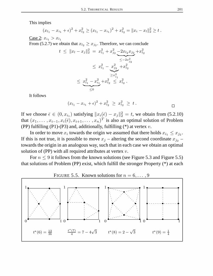
5.2. THEORETICAL RESULTS 201
This implies
(xl1 − xi1 + ε)2 + x2l2 ≥ (xl1 − xi1)
2 + x2l2 = ‖xi − xl‖2
2 ≥ t .
Case 2: xi1 > xl1
From (5.2.7) we obtain thatxl2 ≥ xj2 . Therefore, we can conclude
t ≤ ‖xl − xj‖22 = x2
l1 + x2j2 −2xl2xj2︸ ︷︷ ︸
≤−2x2j2
+x2l2
≤ x2l1 − x2
j2︸︷︷︸≥x2
i1
+x2l2
≤ x2l1 − x2
i1︸ ︷︷ ︸≤0
+x2l2 ≤ x2
l2 .
It follows
(xl1 − xi1 + ε)2 + x2l2 ≥ x2
l2 ≥ t .2
If we chooseε ∈ (0, xi1) satisfying‖xi(ε) − xj‖22 = t, we obtain from (5.2.10)that (x1, . . . , xi−1, xi(ε), xi+1, . . . , xn)T is also an optimal solution of Problem(PP) fulfilling (P1)-(P3) and, additionally, fulfilling (*) at vertexv.
In order to movexi towards the origin we assumed that there holdsxi1 ≤ xj2 .If this is not true, it is possible to movexj – altering the second coordinatexj2 –towards the origin in an analogous way, such that in each case we obtain an optimalsolution of (PP) with all required attributes at vertexv.
Forn ≤ 9 it follows from the known solutions (see Figure 5.3 and Figure 5.5)that solutions of Problem (PP) exist, which fulfill the stronger Property (*) at each
FIGURE 5.5. Known solutions forn = 6, . . . , 9
1
1
0
t?(6) = 1336
10
1
t?(7)4
= 7 − 4√
3
0 1
1
t?(8) = 2 −√3
0 1
1
t?(9) = 14

202 PACKING EQUAL CIRCLES IN A SQUARE
vertexv of U with Property (P3b). Hence, we have to verify the existence of suchpoints only forn ≥ 10. This implies that there holdst = t?(n) ≤ 0.25 and thus
S2(v, t) ∩ S2(w, t) = ∅ (5.2.11)
for two different verticesv andw of the unit square. Therefore, we can apply theargumentation used above in order to guarantee that (*) is fulfilled at each vertexof U , which has Property (P3b). Property (5.2.11) implies that the points we wouldlike to move in order to enforce (*) must be different for different vertices ofU .
�
In the following we denote by Property (P3) this stronger version.
5.2.2. Properties of an Optimal Solution along each Edge.If we considerthe behavior of an optimal solution on the boundary lines of the unit squareU , wecannot expect that two consecutive points have exactly the optimal distance (com-pare, e.g., the optimal solutions forn = 6 or n = 7, see [SM65] or Figure 5.5).We are only able to verify the existence of an optimal solution with the propertythat this distance is smaller than two times the optimal one. This is the result of thefollowing theorem. At first, however, one additional lemma is needed in order toestablish this statement.
LEMMA 5.2.5. Let (x1, . . . , xn)T ∈ IR2n be an optimal solution of Problem(PP) with optimal valuet?(n). Assume further that there exist indicesi, j ∈ {1, . . . , n} andl ∈ {1, 2} satisfying
‖xi − xj‖22 ≥ 4t?(n) and xil = xjl ∈ {0, 1} , (5.2.12)
and, moreover, that there does not exist an indexk ∈ {1, . . . , n} \ {i, j} withxk ∈ [xi, xj ]. Then there holds
intU ∩ {x1, . . . , xn} 6= ∅ . (5.2.13)
This means, if two consecutive pointsxi andxj lying on the same boundary line ofthe unit squareU have a distance not smaller than two times the optimal distance√t?(n), then there exists a memberxm of this optimal solution belonging to the
interior ofU .
PROOF: The pointsxi andxj belong by Assumption (5.2.12) to the sameedge ofU . Hence there holds
‖xi − xj‖22 ≤ 1
and consequently regarding the left part of (5.2.12) we knowt?(n) ≤ 0.25.

5.2. THEORETICAL RESULTS 203
We prove Relation (5.2.13) by contradiction. Assume that there does not exista member of the optimal solution belonging to the interior ofU . With respect tothe value oft?(n) we distinguish again two cases.
Case 1: t?(n) = 0.25From the first part of (5.2.12) it follows that‖xi − xj‖22 = 1 and thus these pointsare vertices ofU . It can be seen that in this situationn cannot be greater than7.Indeed, it is not possible to place more points on the boundary lines ofU such thatthe squared distance is not smaller than0.25. However, forn ≤ 7 solutions withlarger minimum distances are known [SM65] (see also Figures 5.3 and 5.5). Con-sequently, the feasible point(x1, . . . , xn)T is not optimal for (PP), contradictingthe assumption.
Case 2: t := t?(n) < 0.25In this case it is possible to explicitly construct a pointx = (x1, . . . , xn)T with abigger minimum squared distance thant.
Assume, without loss of generality, that there holdsi = n andj = 1 and thatthe membersxi (i = 1, . . . , n) are numbered in such a way thatxi+1 is a directneighbor ofxi (compare with Figure 5.6). Denote, fori ∈ {1, . . . , n − 1}, by
FIGURE 5.6. Numbering
xn x1
x2
x3
x4
xn−1
xn−2
xn−3
di,i+1 the 1-norm distance between the two consecutive pointsxi andxi+1, i.e.,
di,i+1 := ‖xi − xi+1‖1 ≥ ‖xi − xi+1‖2 ≥√t . (5.2.14.a)
Denote, furthermore, bydn,1 the according distance betweenxn andx1, i.e.,
dn,1 := ‖xn − x1‖1 ≥ ‖xn − x1‖2 ≥ 2√t . (5.2.14.b)

204 PACKING EQUAL CIRCLES IN A SQUARE
Since the total length of the boundary lines ofU is 4 it follows that there holdsn−1∑i=1
di,i+1 + dn,1 = 4 .
Therefore, from (5.2.14.a) and (5.2.14.b) we obtain
(n+ 1)√t ≤ 4 . (5.2.15)
Set
δ :=4
n+ 0.5−√t .
From Relation (5.2.15) we see that
0 < δ
and because ofn ≥ 8 (compare with Case 1) we know that
δ < 0.5−√t .
In the sequel we construct now a solutionx = (x1, . . . , xn)T of Problem (PP) witha minimum pairwise distance of
√t+ δ. In order to do this we will place one point
at the center ofU and the remaining (n− 1) points will be placed at the boundaryof the unit square. Let us first interpret the edges ofU as one connected line, i.e.,as the interval[0, 4], where each integer in this interval coincides with a vertex ofU . 0 and4 coincide with the same vertex, namely the origin. We construct nowa sequence of (n − 1) real numbers lying inside this interval in such a way thattwo successive numbers have a distance equal to
√t+ δ, if no integer lies between
them, and a distance equal to√
2(√t + δ) otherwise. This is sufficient in order to
obtain a solution of Problem (PP) with a minimum distance in the Euclidean normnot smaller than
√t+ δ, as required.
The needed sequence of real numbers is defined as follows
x1 := 0.0
and, fori ∈ {2, . . . , n− 1},
xi :=
{xi−1 + (
√t+ δ) , if bxi−1c = bxi−1 + (
√t+ δ)c
xi−1 +√
2(√t+ δ) , otherwise.
In order to verify that this sequence has the claimed properties it is sufficient toshow thatxn−1 lies in the interval[0, 4] and, additionally, thatxn−1 has a distancenot smaller than
√t + δ to 4 (and hence to the origin). If we look for the biggest
5.2. THEORETICAL RESULTS 205
quantityk ∈ IN of numbers constructed by the foregoing prescription, which be-long to the interval[0, 4− (
√t+ δ)], then we have to solve the problem
max k
(k − 4)(√t+ δ) + 3
√2(√t+ δ) ≤ 4− (
√t+ δ)
k ∈ IN .
Note that there are three integers inside the interval[0, 4]. Hence there are at mostthree pairs(xi, xi+1) (i ∈ {1, . . . , k − 1}) with a distance of
√2(√t + δ). The
remaining(k − 4) distances are by construction equal to(√t + δ). From the
properties ofδ it is easy to verify that we obtaink? = n − 1, wherek? is theoptimal solution of the previous problem.
With this sequence of real numbers we are now able to construct the requiredfeasible pointx ∈ Un with the claimed minimal pairwise distance. Set, fori = 1, . . . , n− 1,
xi :=
(xi, 0.0)T , if 0.0 ≤ xi ≤ 1.0
(1.0, xi − 1.0)T , if 1.0 < xi ≤ 2.0
(1.0− (xi − 2.0), 1.0)T , if 2.0 < xi ≤ 3.0
(0.0, 1.0− (xi − 3.0))T , otherwise.
Adding xn := (0.5, 0.5)T we obtain obviously a feasible point for (PP). Straight-forward calculation shows that this point has a larger minimum squared distancethan(x1, . . . , xn)T . This contradicts the optimality of(x1, . . . , xn)T and com-pletes the proof. �
If two consecutive points of an optimal solution of Problem (PP) lying on thesame edge ofU have a distance bigger than or equal to two times the optimal one,the previous lemma guarantees that there always exists a member of this optimalsolution belonging to the interior of the unit squareU . In the proof of the next theo-rem we show that it is possible to move one of these interior points to the boundaryof U without decreasing the minimum distance. This leads to the existence of anoptimal solution of Problem (PP) with the claimed property at each boundary lineof the unit squareU .

206 PACKING EQUAL CIRCLES IN A SQUARE
THEOREM 5.2.6. There exists an optimal solution(x?1, . . . , x?n)T of Problem
(PP) with the following property:
If there exist indicesi, j ∈ {1, . . . , n}with i 6= j and an indexl ∈ {1, 2}withx?il =x?jl ∈ {0, 1} and, furthermore, there does not exist an indexk ∈ {1, . . . , n}\{i, j}with x?k ∈ [x?i , x
?j ], then there holds
‖x?i − x?j‖22 < 4t?(n) . (P4)
I.e., two consecutive members of(x?1, . . . , x?n)T belonging to the same edge of theunit square have a distance smaller than two times the optimal one.
PROOF: Let (x1, . . . , xn)T ∈ IR2n be an optimal solution of Problem (PP)with optimal valuet := t?(n). Assume that there exist two consecutive membersof this optimal solution with a distance not smaller than two times the optimal one.This means that there exist indicesi, j ∈ {1, . . . , n}, i 6= j and an indexl ∈ {1, 2}satisfying
‖xi − xj‖22 ≥ 4t (5.2.16.a)and
xil = xjl ∈ {0, 1} , (5.2.16.b)
and there does not exist an indexk ∈ {1, . . . , n} \ {i, j} such thatxk belongs to[xi, xj ]. As long as there are two consecutive points with Properties (5.2.16.a) and(5.2.16.b), Lemma 5.2.5 yields that there exists a member of(x1, . . . , xn)T locatedwithin the interior ofU . In order to prove the existence of an optimal solution withProperty (P4) it is hence sufficient to show that we are able to move one of theseinterior points to the boundary ofU without decreasing the minimum distance.
Without loss of generality, we assumei = 1, j = 2, l = 2, x12 = x22 = 0.0andx11 < x21 , i.e.,x1 andx2 lie on the edgee = {y ∈ IR2 : 0.0 ≤ y1 ≤ 1.0,y2 = 0.0} and there holdsx21 ≥ x11 + 2
√t.
Denote by
A := {xi : i ∈ {3, . . . , n}, xi1 ≤ x11 or xi1 ≥ x21}the set of all members of(x1, . . . , xn)T different fromx1 andx2 with the propertythat the first coordinate does not belong to the open interval(x11 , x21). It is easy toverify that, for eachλ ∈ [x11 +
√t, x21 −
√t] andx ∈ A, there holds
‖x− (λ0)‖22 ≥ t . (5.2.17)
Depending on the structure of setA we distinguish two cases.
5.2. THEORETICAL RESULTS 207
Case 1: {x3, . . . , xn} \A = ∅Set
x?31:=
x11 + x21
2and x32 := 0.0 .
From (5.2.17) we obtain, for eachk ∈ {4, . . . , n},‖x?3 − xk‖22 ≥ t .
Moreover, fori ∈ {1, 2}, there holds also‖x?3 − xi‖22 ≥ t. Therefore, the point(x1, x2, x
?3, x4, . . . , xn)T is another optimal solution of (PP) with the property that
the number of members belonging to the boundary ofU is increased by one – incomparison with(x1, . . . , xn)T .
Case 2: {x3, . . . , xn} \A 6= ∅Choose an indexl ∈ {3, . . . , n} such that there holds
xl2 = min{y2 | y ∈ {x3, . . . , xn} \A} . (5.2.18)
Construct a new pointx?l ∈ IR2 belonging to[x1, x2] according to the followingrule
x?l1 :=
xl1 , if x11 +
√t ≤ xl1 ≤ x21 −
√t
x11 +√t , if xl1 < x11 +
√t
x21 −√t , otherwise
and x?l2 := 0.0 .
For i ∈ {1, 2} there holds obviously‖x?l − xi‖22 ≥ t. In order to finish the proofwe have to show that the pointx?l has a squared distance not smaller thant to anymember of(x1, . . . , xn)T belonging to the set
A := {x3, . . . , xn} \ (A ∪ {xl}) .
Choose an arbitrary, but fixed elementxk of A. Depending on the definition ofx?l1 it is necessary to distinguish three subcases.
Case 2.1: x?l1 = xl1
From (5.2.18) we know thatxk2 ≥ xl2 . It follows
‖xk − x?l ‖22 = (xk1 − xl1)2 + x2k2
≥ (xk1 − xl1)2 + (xk2 − xl2)2= ‖xk − xl‖22 ≥ t .

208 PACKING EQUAL CIRCLES IN A SQUARE
Case 2.2: x?l1 = x11 +√t
The following assertions are true
xl2 ≤ xk2 (compare with Relation (5.2.18)) (5.2.19.a)
xl1 − x11 <√t (definition ofx?l1 ) (5.2.19.b)
x11 ≤ xl1 (sincexl /∈ A) (5.2.19.c)
t ≤ ‖xk − xl‖22 = (xk1 − xl1)2 + (xk2 − xl2)2 (5.2.19.d)
t ≤ ‖xl − x1‖22 = (x11 − xl1)2 + x2l2 . (5.2.19.e)
Using these statements we can conclude for the squared distance betweenx?l andxk
‖xk − x?l ‖22 = (xk1 − x11 −√t)2 + x2
k2
= [(xk1 − xl1) + xl1 − x11 −√t]2 + [(xk2 − xl2) + xl2 ]
2
= (xk1 − xl1)2 + 2(xk1 − xl1)(xl1 − x11 −√t)
+ (xl1 − x11)2 − 2
√t(xl1 − x11) + t
+ (xk2 − xl2)2 + 2xl2 (xk2 − xl2)︸ ︷︷ ︸≥0, (5.2.19.a)
+x2l2
≥ (xk1 − xl1)2 + (xk2 − xl2)2 + ‖xl − x1‖22︸ ︷︷ ︸≥t, (5.2.19.e)
+t
+ 2(xk1 − xl1)(xl1 − x11 −√t) + 2(x11 − xl1)
√t
≥ 2t+ (xk1 − xl1)2 + (xk2 − xl2)2+ 2(xk1 − xl1)(xl1 − x11 −
√t) + 2(x11 − xl1)
√t
=: C
We need thatC is not smaller thant. In order to prove this we have todistinguish two further subcases.
Case 2.2.1: xk1 − xl1 ≤ √t
In this situation we obtain
C = 2t + ‖xk − xl‖22 + 2[(xk1 − xl1)︸ ︷︷ ︸
≤√t
(xl1 − x11 −√
t)︸ ︷︷ ︸≤0, (5.2.19.b)
+(x11 − xl1)√
t]
≥ 2t + ‖xk − xl‖22 + 2
√t [xl1 − x11 −√
t + x11 − xl1 ]︸ ︷︷ ︸=−√
t
= ‖xk − xl‖22 ≥ t (see (5.2.19.d)).

5.3. THE ALGORITHM 209
Case 2.2.2: xk1 − xl1 >√
t
It follows
C = 2t + (xk1 − xl1)2 + (xk2 − xl2)
2︸ ︷︷ ︸≥0
+ 2[(xk1 − xl1)(xl1 − x11 −√
t) + (x11 − xl1)︸ ︷︷ ︸≤0, (5.2.19.c)
√t︸︷︷︸
<(xk1−xl1 )
]
≥ 2t + (xk1 − xl1)2 − 2
√t(xk1 − xl1)
= (xk1 − xl1 −√
t)2︸ ︷︷ ︸≥0
+t ≥ t .
Hence we obtain in Case 2.2 that‖xk − x?l ‖22 ≥ t.Case 2.3: x?l1 = x21 −
√t
By analogous calculations as in Case 2.2 it is possible to conclude
‖xk − x?l ‖22 ≥ t .
We showed that, for each indexk ∈ {1, . . . , n} \ {l}, there holds
‖x?l − xk‖22 ≥ t .
Therefore, the point(x1, . . . , xl−1, x?l , xl+1, . . . , xn)T is also an optimal solution
of Problem (PP) with the same additional property as the new solution constructedin Case 1. �
The results of Theorem 5.2.3 in connection with Corollary 5.2.4 and the resultof Theorem 5.2.6 are independent from each other. Combining both we know thatthere exists an optimal solution(x?1, . . . , x?n)T of Problem (PP) fulfilling Properties(P1)-(P4). In particular, as we will see in Section 5.5, Property (P4) and the strongversion of Property (P3) give us a powerful tool in order to reduce the dimensionof subproblems in a rectangular branch-and-bound algorithm.
5.3. The Algorithm
After the derivation of the theoretical results in the previous section giving usmore insight into the structure of possible solutions of Problem (PP) we presentnow an algorithm for solving (PP). As in the solution approaches for (QP) devel-oped in Chapters 3 and 4 we use a branch-and-bound scheme (see also Subsection1.2.2). In Chapter 3 we saw that the use of simplices as subdivision sets can lead

210 PACKING EQUAL CIRCLES IN A SQUARE
to a faster solution approach than the application of hyperrectangles, in particular,if we try to solve all-quadratic problems with a large number of constraints. Eventhough Problem (PP) has – in comparison with the dimension – a large numberof constraints we prefer in the following algorithm hyperrectangles as subdivisionsets. Using this type of sets the required initial hyperrectangle (see again Subsec-tion 1.2.2) is immediately given byUn. Moreover, the strategies, which we willdevelop in subsequent sections in order to improve the numerical performance ofour solution scheme for (PP), need hyperrectangles.
In the present section we describe the basic algorithm without expatiating thedetails. These are discussed in the following sections. The presented algorithmguarantees to detect for a prespecified toleranceε > 0 anε-optimal solution for thepoint scattering problem in finite time. Some preliminary notes about the conver-gence of our approach are given at the end of this section.
Denote byf : IR2n → IR
f(x) := min1≤i<j≤n
‖xi − xj‖22the minimum pairwise squared distance of the membersxi = (xi1 , xi2)T
(i ∈ {1, . . . , n}) of a 2n-dimensional pointx = (x1, . . . , xn)T ∈ IR2n. Usingthis notation Problem (PP) can be written as
max f(x)
x ∈ Un .(PP)
Assume that a pointx ∈ Un is known withf(x) > 0. We can generate sucha point x by using a local optimizer alone or in combination with a stochasticalapproach like a multi-start algorithm (see, e.g., [BR95] for an introduction to sto-chastic methods for global optimization). However, it is not necessary thatx isa local optimal point for Problem (PP). Therefore, it is also sufficient to simplyconstructx ∈ Un geometrically.
Assume further that an upper boundµ for the optimal valuet?(n) of Problem(PP) is given. If the optimal valuet?(n− 1) for Problem (PP) withn− 1 points oran upper bound fort?(n− 1) is known, we can choose this value forµ. Otherwiseit is possible to setµ := 2.0 since, for anyx ∈ Un, there holds0 ≤ f(x) ≤ 2.
Similar to Algorithm 3.1 and Algorithm 4.1 the formulation of the algorithmfor Problem (PP) follows nearly the guidelines of a basic branch-and-boundschemegiven in [HPT95, Algorithm 3.5]. Note that the following algorithm has specialadaptations to Problem (PP). In particular, we do not insist that the union of all

5.3. THE ALGORITHM 211
partition sets forms the full set (see (5.3.1) below). Since the details of the followingapproach will be expatiated later in this chapter, we use another type of descriptionthan before.
ALGORITHM 5.1 (Rectangular Branch-and-Bound Algorithm for (PP) ).
InitializationChoose a real numberε ≥ 0.Set, for i ∈ {1, . . . , n}, R0
i ← [0, 1] × [0, 1] =: [l0i1 , L0i1 ] × [l0i2 , L
0i2 ],
R0 ← R01 × . . .×R0
n ⊂ IR2n, R0 ← {R0},x0 ← x, η0 ← f(x0), Q← {x0}, µ0 ← µ, µR0 ← µ0, k ← 0.
Loop
Step I: (Stopping criterion)If there holdsµk − ηk ≤ ε, thenSTOP.x? := xk is anε-optimal solution of Problem (PP), i.e.,t?(n)− ηk = t?(n)− f(xk) ≤ ε.
Step II:Choose the smallest indexj ∈ {1, . . . , n} satisfying
max{Lkj1 − lkj1 , Lkj2 − lkj2} =
max{max{Lki1 − lki1 , Lki2 − lki2}, i = 1, . . . , n
}.
Step III: (Subdivision strategies)Constructl ∈ IN two-dimensional rectanglesRk1j , . . . , R
klj with equal size
fulfilling, for eachi = 1, . . . , l,
Rki
j ⊂ Rkj
and, for each1 ≤ i < p ≤ l,intRki
j ∩ intRkp
j = ∅ .
Step IV: (Size reduction strategies)If possible, reduce, for eachi ∈ {1, . . . , l}, the size of the hyper-rectangles
Rki = Rk1 × . . .×Rkj−1 ×Rki
j ×Rkj+1 × . . .×Rkn ,
i.e., construct hyperrectanglesRki ⊂ Rki .

212 PACKING EQUAL CIRCLES IN A SQUARE
Step V: (Upper bounds)For p = 1 To l Do
If Rkp = ∅ ThenµRkp ← −∞
ElseConstruct an upper boundµRkp for the optimization problem
max t
t− ‖xi − xj‖22 ≤ 0 1 ≤ i < j ≤ n(x1, . . . , xn)T ∈ Rkp
ηk ≤ t ≤ µk .
(SP)
Use each pointy ∈ Rkp found during the calculation ofµRkp in orderto update the lower bound, i.e.,
ηk ← max{ηk, f(y)}Q ← Q ∪ {y} .
EndIfEndFor
Step VI:Adjust the setRk of relevant subdivision sets by setting
Rk ← (Rk \Rk) ∪ {Rkp : p ∈ {1, . . . , l} with µRkp ≥ ηk} .
Step VII: (Pruning rule)Rk+1 ← {R ∈ Rk : µR ≥ ηk}
Step VIII:Update the lower and the upper bound by setting
ηk+1 ← ηk
µk+1 ←{
max{µR : R ∈ Rk+1} , if Rk+1 6= ∅ηk+1 , otherwise
.
Choose a new nodeRk+1 of the partition tree satisfyingµRk+1 = µk+1.Select a pointxk+1 ∈ Q with f(xk+1) = ηk+1. k ← k + 1.Go to Step I.

5.3. THE ALGORITHM 213
REMARK 5.3.1. Problem (PP) is a maximization problem. Therefore, wehave changed in contrast to the previous algorithms the meaning of the Greek sym-bolsη andµ. In Algorithm 5.1η denotes a lower bound andµ is an upper bound.
As mentioned before, the formulation of Algorithm 5.1 follows nearly theguidelines of a general branch-and-bound scheme given in [HPT95]. There aretwo main ways in order to adapt this general algorithm to a special problem orproblem class. First of all it is necessary to decide how the bounds should be con-structed. For the lower boundsηk (k ∈ IN) we use the most common and simpleidea, which we also used in Algorithm 3.1 and Algorithm 4.1 for the boundsηk.The lower bound is updated each time the algorithm generates a new pointy ∈ IR2n
belonging to the feasible region of (PP) with a function valuef(y) bigger than thecurrent boundηk.
In the construction of the upper boundµR with respect to a given hyperrect-angleR we invest more effort. Similar to the solution approaches for (QP) wecalculate this bound by solving an LP-relaxation of Problem (PP) with the addi-tional constraint(t, x) ∈ [ηk, µk] × R (see Subproblem (SP) in Step V). By in-terpreting Problem (SP) as an all-quadratic problem or as a polynomial problemwe could choose the LP-relaxations proposed in [AKLV95] or [ST92] (see alsoSection 1.3). However, doing this we do not stay abreast of the special structure of(SP). Note that each quadratic constraint depends only on the four variablesxi1 ,xi2 , xj1 andxj2 . Exploiting this structure we are able to construct a better linearapproximation of the feasible region of Problem (SP) than by using one of thesegeneral approaches. In Section 5.4 our method for calculating upper bounds forthis special problem is discussed.
The second step of adapting a general branch-and-bound scheme is to deter-mine in which way we subdivide the current subdivision set. In Algorithm 3.1 andAlgorithm 4.1 we used radial subdivisions of the appliedn-simplices (see Defi-nition 1.2.2), which result in a partition (Definition 1.2.1) of the subdivided set.The hyperrectangleRk used in Algorithm 5.1 is the Cartesian product ofn two-dimensional rectanglesRki (i ∈ {1, . . . , n}). We partitionRk by splitting one ofthese rectanglesRki . In Step II we decide which rectangleRki (i ∈ {1, . . . , n})we would like to subdivide and in Step III we use a strategy to generatel ∈ INrectangular subsets ofRki . How we do this is described in Section 5.5. Our strategyis similar to the well-known bisection approach (see, e.g., page 101). However, in

214 PACKING EQUAL CIRCLES IN A SQUARE
contrast to this strategy we divideRk in each iteration with respect to two dimen-sions and not only regarding one dimension. Furthermore, exploiting the structureof Problem (PP) we are able to eliminate a lot of possible partition sets in advanceeven without computing upper bounds. Therefore – at the end of Step III – the setsRk1 , . . . , Rkl do not form a partition ofRk. The property
l⋃i=1
Rki = Rk ⇔l⋃i=1
Rki
j = Rkj (5.3.1)
is not necessarily satisfied (compare with the required properties in Step III).In branch-and-bound algorithms derived for general problem classes it is usu-
ally not possible to manipulate the current subdivision setRk apart from its split-ting. In Algorithm 3.1 and Algorithm 4.1 we do not know how to manipulate furtherthen-simplicesSkj resulting from the partition of the current setSk, since in gen-eral no additional information about the structure of Problem (QP) is available. If abranch-and-bound scheme is developed for a special problem instance, as it is thecase for Algorithm 5.1, then exploiting the structure of this instance could enable usto derive manipulation strategies for the sets resulting after the subdivision step. Infact, in the case of Problem (PP) we can reduce under some circumstances the sizeof the relevant hyperrectanglesRki using the theoretical results derived in Section5.2 and the knowledge of the current best known valueηk, as mentioned in Step IVof the algorithm. The resultingsize reduction strategiesare presented in Section5.6.
Before expatiating the details of the suggested algorithm in the following sec-tions let us first give some notes on the convergence of this approach. We wouldlike to formulate three conditions, which have to be satisfied by the upper bounds(Step V) and by the subdivision set manipulation strategies, i.e., by the subdivisionstrategies and the size reduction strategies (Step III and Step IV). Using these con-ditions we are able to prove the convergence of our method.
The conditions are as follows.
(C1) The subdivision strategy is exhaustive, i.e., for each infinite sequence ofhyperrectangles{Rk}k∈IN satisfyingRk+1 ⊂ Rk for eachk ∈ IN, thereexists a points ∈ Un with
limk→∞
Rk =⋂k∈IN
Rk = {s}
(compare with Definition 4.3.1).

5.3. THE ALGORITHM 215
(C2) If an infinite nested sequence of hyperrectangles{Rk}k∈IN with the prop-erty limk→∞Rk = {s} ⊂ Un is given, then there holds
limk→∞
µRk = f(s) .
(C3) The subdivision strategies and the size reduction strategies areconsistentinthe following sense. LetP k ⊂ Un be the union of the relevant subdivisionsets in Step I in iterationk ∈ IN, i.e.,P k =
⋃R∈Rk R. Then there holds
thatP k ∪Q contains an optimal solution of Problem (PP), i.e.,(P k ∪Q) ∩ SOL(n) 6= ∅
whereSOL(n) denotes the set of optimal solution of Problem (PP) withn
scattering points.
Condition (C1) for the subdivision strategy and Condition (C2) for the up-per bounds are often used in order to prove the convergence of branch-and-boundschemes for general problem classes (see, e.g., [HPT95, Section 3.7]). Note that inthe convergence proof for Algorithm 3.1 (see Section 3.4) and in the convergenceproof for Algorithm 4.1 in the exhaustive case (see Section 4.3) we have just veri-fied these conditions. In both algorithms we had the property that the sets resultingfrom the subdivision of the currentn-simplex form a partition ofSk and that thesesets are not further manipulated. Therefore, these two conditions were sufficientfor the convergence of these approaches.
As mentioned before, the subdivision strategy used in Step III of Algorithm5.1 does not lead to a partition, since Relation (5.3.1) is not necessarily satisfied.Moreover, we are able to reduce the size of the hyperrectanglesRk1 , . . . , Rkl withour size reduction strategies in Step IV. Therefore, in order to prove the correct-ness of Algorithm 5.1 in the sense that this method detects anε-optimal solutionof Problem (PP), it is not sufficient that Condition (C1) and Condition (C2) arefulfilled. In Section 5.5 and in Section 5.6 we will see that using our subdivisionset manipulation strategies we may lose optimal solutions, i.e., we cut away partsof the feasible region of Problem (PP) containing optimal solutions without detect-ing them. However, as long as the strategies applied in our method guarantee thatthere still exist at least one optimal solution in the part of the feasible area of (PP),which is not eliminated by the set manipulation strategies, we are able to prove thecorrectness of Algorithm 5.1. If Algorithm 5.1 fulfills Condition (C3), it is ensuredthat not all optimal solutions are eliminated without detecting them.

216 PACKING EQUAL CIRCLES IN A SQUARE
Under the assumption that the required conditions are satisfied by the strategiesused in Algorithm 5.1 we are able to show that our method detects in finite timean ε-optimal solution of Problem (PP), ifε is chosen greater than0. This willbe a direct consequence of the following convergence theorem, which proves thecorrectness of Algorithm 5.1 for the caseε = 0.
THEOREM 5.3.1. Assume thatε = 0 and that Algorithm 5.1 fulfills Condi-tions (C1), (C2) and (C3). Then the following assertions are true:
(i) If Algorithm 5.1 stops after a finite number of iterations withηk = µk, thenit follows thatxk is an optimal solution of Problem (PP) with optimal valueηk.
(ii) If Algorithm 5.1 generates an infinite point sequence{xk}k∈IN, then thereholds that each accumulation pointx? of this sequence is an optimal solu-tion of Problem (PP) with optimal valuef(x?).
PROOF: Denote, fork ∈ IN, by P k the part ofUn still to be analyzed inStep I of iterationk, i.e.,
P k =⋃R∈RkR .
From the description of the algorithm it follows immediately that, for anyk ∈ IN,
f(xk) = ηk ≤ maxx∈Pk∪Q
f(x) = max{ max(t,x)∈Fk
t , maxx∈Q
f(x)︸ ︷︷ ︸=ηk
} (5.3.2)
with F k = {(t, x) ∈ IR× P k with t− ‖xi − xj‖22 ≤ 0 , 1 ≤ i < j ≤ n}, and
maxx∈Pk∪Q
f(x) ≤ µk . (5.3.3)
Since Condition (C3) is satisfied for eachk ∈ IN, there holds
maxx∈Pk∪Q
f(x) = t?(n) . (5.3.4)
Combining (5.3.2), (5.3.3) and (5.3.4) we obtain the first result (i).
In order to prove (ii) we can use the general convergence theory proposedin [HPT95, Section 3.7]. Because of Property (C3) our algorithm has the sameessential properties as the general branch-and-bound scheme used in [HPT95, Al-gorithm 3.5]. Note that we are interested in detecting oneglobal solution of Prob-lem (PP). Therefore, assertion (ii) follows immediately from [HPT95, Theorem

5.3. THE ALGORITHM 217
3.8], if for each infinite nested subsequence{Rkq}q∈IN of the generated sequence{Rk}k∈IN of 2n-dimensional hyperrectangles, there holds
limq→∞[µRkq − ηkq ] = 0 . (5.3.5)
Let {Rkq}q∈IN be a subsequence of{Rk}k∈IN satisfyingRkq+1 ⊂ Rkq for eachq ∈ IN. From Condition (C1) we know that in this situation there exists a points ∈ Un with
limq→∞Rkq = {s} . (5.3.6)
Algorithm 5.1 generates, for eachq ∈ IN, a pointykq ∈ Rkq satisfying
f(ykq) ≤ ηkq .
Note that in Step V at least one point belonging toRkq (q ∈ IN) is used for updatingthe lower boundηkq . From (5.3.6) we obtain hence
limq→∞ f(ykq) = f(s) ≤ lim
q→∞ ηkq . (5.3.7)
Condition (C2) implies thatlimq→∞µRkq = f(s) . (5.3.8)
Using (5.3.7) and (5.3.8) Property (5.3.5) follows readily. �
REMARK 5.3.2. In the convergence proofs for Algorithm 3.1 and Algorithm4.1 in the exhaustive case it was not possible to use the general convergence theorygiven in [HPT95, Section 3.7] (see Remark 3.4.1(b)). In both approaches we do notnecessarily generate feasible points for each considered subdivision set. Therefore,we do not know how the sequence{ηk}k∈IN behaves. Since in Algorithm 5.1we consider the formulation of Problem (PP) given on page 210 we can use eachpoint belonging to the current hyperrectangle in order to update the lower boundηk (k ∈ IN). This guarantees that the sequence{ηk}k∈IN converges to the optimalvaluet?(n) in the infinite case.
As a consequence of the convergence result presented above it is immediatelyclear that, for eachε > 0, Algorithm 5.1 generates anε-optimal solutionxk infinite time. In the following sections we describe the details of the calculationof the upper bounds and the details of the diverse subdivision set manipulationstrategies, which we used in our implementation of Algorithm 5.1. In order toguarantee a correct functioning of the suggested approach we will have to show atthe respective places that the postulated conditions are fulfilled.
218 PACKING EQUAL CIRCLES IN A SQUARE
5.4. Upper Bounds
In this section we describe the calculation of an upper bound for the optimiza-tion problem
max t
t− ‖xi − xj‖22 ≤ 0 1 ≤ i < j ≤ nxi ∈ Ri i = 1, . . . , n
η ≤ t ≤ µ ,
(SP’)
where, fori ∈ {1, . . . , n}, Ri = [li1 , Li1 ] × [li2 , Li2 ] (0 ≤ lij ≤ Lij ≤ 1,j ∈ {1, 2}) is a two-dimensional rectangle, andη > 0 andµ ≤ 4 are real numbers.This problem coincides with Subproblem (SP) in the description of Algorithm 5.1in the previous section.
We calculate an upper bound of (SP’) by solving an LP-relaxation of this prob-lem. In order to obtain such a relaxation we need for any concave quadratic con-straint
t− ‖xi − xj‖22 ≤ 0
(1 ≤ i < j ≤ n) a piecewise affine convex functionhij : IR × IR2 × IR2 → IRwith the property
{(t, xi, xj)T ∈ [η, µ]×Ri ×Rj : t− ‖xi − xj‖22 ≤ 0}⊂ {(t, xi, xj)T ∈ [η, µ]×Ri ×Rj : hij(t, xi, xj) ≤ 0} .
(5.4.1)
In order to simplify the presentation we ignore at first the indicesi, j and considerone concave quadratic constraint
g(t, x, y) := t− ‖x− y‖22 ≤ 0 ,
where(t, x, y)T is restricted to the set[η, µ]×Rx ×Ry with
Rx := [lx1 , Lx1 ]× [lx2 , Lx2 ]and
Ry := [ly1 , Ly1 ]× [ly2 , Ly2 ] .
In order to construct a piecewise affine convex functionh such that
F := {(t, x, y)T ∈ [η, µ]×Rx ×Ry : t− ‖x− y‖22 ≤ 0}⊂ {(t, x, y)T ∈ [η, µ]×Rx ×Ry : h(t, x, y) ≤ 0} ,
(5.4.2)

5.4. UPPERBOUNDS 219
let us examine the quadratic part ofg, i.e., consider the functiong : IR2× IR2 → IRgiven by
g(x, y) := ‖x− y‖22 = (x1 − y1)2 + (x2 − y2)2over the4-dimensional rectangleR := Rx × Ry. Substitutingv for the term(x1 − y1) andw for (x2 − y2) we can interpretg as a two-dimensional functiong : IR2 → IR with
g(v, w) := v2 + w2 .
According to the feasible region ofx andy the new variables are restricted as fol-lows
−1 ≤ lv := lx1 − Ly1 ≤ v ≤ Lx1 − ly1 =: Lv ≤ 1
−1 ≤ lw := lx2 − Ly2 ≤ w ≤ Lx2 − ly2 =: Lw ≤ 1 .
If a piecewise affine functionh : IR2 → IR with the properties
• h is concave, i.e., the minimum of a finite number of affine functions,• there holds, for any
(vw
) ∈ R := [lv, Lv]× [lw, Lw],
h(v, w)
{≥ µ , if g(v, w) ≥ µ≥ g(v, w) , if η ≤ g(v, w) < µ
, (5.4.3)
is given, we obtain by setting
h(t, x, y) := t− h(x1 − y1, x2 − y2)a functionh fulfilling (5.4.2). Note that if there is a point(t, x, y)T ∈ [η, µ]×Rx×Ry with g(x, y) ≥ µ andg(t, x, y) ≤ 0, then – regarding (5.4.3) – there holdsh(x1 − y1, x2 − y2) ≥ µ and henceh(t, x, y) ≤ 0. Note further that there does notexist a point(t, x, y)T ∈ [η, µ]×Rx ×Ry with g(x, y) < η andg(t, x, y) ≤ 0.
In the next part of this section we describe the construction of a piecewiseaffine concave functionh with Property (5.4.3) in detail. Denote by
V (R) = {(lvlw
),
(Lvlw
),
(LvLw
),
(lvLw
)} = {v1, v2, v3, v4}
the set of vertices of the two-dimensional rectangleR and assume, without loss ofgenerality, that there holds
g(v1) = maxz∈R
g(z) . (5.4.4)
Note that a convex function always attains its maximum over a polytopeP in avertex ofP [HPT95, Theorem 1.19].

220 PACKING EQUAL CIRCLES IN A SQUARE
If an affine function : IR2 → IR, `(z) = aT z + b coinciding in three verticesof R with the function values ofg is given, it follows by straightforward calculationthat` also coincides withg in the fourth vertex, i.e., for eachi ∈ {1, . . . , 4}, thereholds
`(vi) = g(vi) . (5.4.5)
PROOF OF(5.4.5): If, for i ∈ {1, 2, 3}, there holds (vi) = g(vi), we obtain
`(v1) = a1lv + a2lw + b = l2v + l2w = g(v1)
`(v2) = a1Lv + a2lw + b = L2v + l2w = g(v2)
`(v3) = a1Lv + a2Lw + b = L2v + L2
w = g(v3) ,
and therefore
g(v4) = l2v + L2w = `(v1) − `(v2) + `(v3)
= a1lv + a2Lw + b = `(v4)2
REMARK 5.4.1. The function is the concave envelope ofg on the rectangle[v1, v2, v3, v4] (see Subsection 1.2.4). Note that the concave envelope of a separablefunction f : IRn → IR, f(x) =
∑ni=1 fi(xi) on a rectangleR = {x ∈ IRn :
li ≤ xi ≤ Li , i = 1, . . . , n} is the sum of the concave envelopes of each partfi : IR→ IR of f on the interval[li, Li] (i = 1, . . . , n) [HT96B, Theorem IV.8].
Because of Relation (5.4.5) it is obvious that the affine function` is an over-estimating function forg on the whole rectangleR, and especially that fulfills(5.4.3). Hence the simplest way in order to obtain the required functionh is to takethe function` itself. However, in some circumstances it is possible to "improve"this overestimator, where "improve" is meant in the sense of a concave approxima-tion of g with respect to the feasible regionF , which has function values smallerthan or equal to. Considering the structure ofF we recognize that it is not neces-sary to overestimateg on the whole rectangleR, as we do by choosing. We onlyneed a concave overestimator for the function
min{µ , g(v, w) } (5.4.6)
on the setR ∩ {(vw) ∈ IR2 : g(v, w) ≥ η} (see Figure 5.7 and compare with
Property (5.4.3)). Note that all points(vw
) ∈ R with a function valueg(v, w)lower thanη (see the bottom of the functiong in Figure 5.7) are infeasible, i.e.,F ∩ {(vw) ∈ IR2 : g(v, w) < η} = ∅.

5.4. UPPERBOUNDS 221
FIGURE 5.7. The relevant function
0
0.2
0.4
0.6
0.8
1
-1
-0.5
0
0.5
1
0
0.1
0.2
0.3
0.4
0.5
0
0.
0
0
v
g(v,w)
w
g(v, w) = min{µ,max{g(v, w), η} }with (v, w)T ∈ [0, 1]× [−1, 1]
Depending on the function values ofg in the vertices ofR ⊂ [−1, 1]× [−1, 1]we distinguish four main cases.
Case 1: g(vi) < η , i ∈ {1, . . . , 4} (see Figure 5.8)
Sinceg is a convex function it follows immediately that, for each(v, w)T ∈ R,there holdsg(v, w) < η. This impliesF = ∅. In this case it is not necessary toconstruct a functionh because we do not need an upper bound for Problem (SP’).
Case 2: g(vi) ≥ µ , i ∈ {1, . . . , 4} (see Figure 5.9(a))
Since, for any(v, w)T ∈ R, there holds
min{µ , max{g(v, w), η} } ≤ µ ,
we obtain by settingh ≡ µ a constant function with Property (5.4.3). This functionis a better approximation ofg with respect to the feasible regionF than the affinefunction`. Moreover, there is no possibility to further improveh without losing the

222 PACKING EQUAL CIRCLES IN A SQUARE
FIGURE 5.8. Case 1
−1
R
v3
1
1
v1
v4
v2
The dotted cir-cle displays thecontourline forg(v, w) = η andthe solid circlefor g(v, w) = µ.
FIGURE 5.9. Case 2 and 3
−1
v2v1
v3v4
R
1
1
(a) Case 2
v4
R
v3
v1 v2
−1
1
1
(b) Case 3
concavity.
Case 3: η ≤ g(vi) ≤ µ , i ∈ {1, . . . , 4} (see Figure 5.9(b))
In this situation the previously defined affine function` is the best approximationof g fulfilling (5.4.3). As in Case 2 it is not possible to improveh ≡ ` and preserve
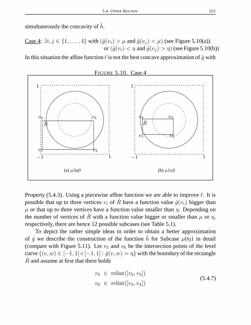
5.4. UPPERBOUNDS 223
simultaneously the concavity ofh.
Case 4: ∃i, j ∈ {1, . . . , 4} with (g(vi) > µ andg(vj) < µ) (see Figure 5.10(a))or (g(vi) < η andg(vj) > η) (see Figure 5.10(b))
In this situation the affine functionis not the best concave approximation ofg with
FIGURE 5.10. Case 4
−1
v4
R
v3
v1 v2
1
1
(a)µ3η0
−1
v1 v2
v3v4
R
1
1
(b) µ1η2
Property (5.4.3). Using a piecewise affine function we are able to improve`. It ispossible that up to three verticesvi of R have a function valueg(vi) bigger thanµ or that up to three vertices have a function value smaller thanη. Depending onthe number of vertices ofR with a function value bigger or smaller thanµ or η,respectively, there are hence 12 possible subcases (see Table 5.1).
To depict the rather simple ideas in order to obtain a better approximationof g we describe the construction of the functionh for Subcaseµ0η1 in detail(compare with Figure 5.11). Letv5 andv6 be the intersection points of the levelcurve{(v, w) ∈ [−1, 1]×[−1, 1] : g(v, w) = η}with the boundary of the rectangleR and assume at first that there holds
v5 ∈ relint([v2, v3])(5.4.7)
v6 ∈ relint([v3, v4])

224 PACKING EQUAL CIRCLES IN A SQUARE
TABLE 5.1. Possible subcases
Subcase |{i ∈ {1, . . . , 4} : g(vi) > µ}| |{i ∈ {1, . . . , 4} : g(vi) < η}|µ0η1 0 1µ0η2 0 2µ0η3 0 3µ1η0 1 0µ1η1 1 1µ1η2 1 2µ1η3 1 3µ2η0 2 0µ2η1 2 1µ2η2 2 2µ3η0 3 0µ3η1 3 1
(for the definition of the relative interior (relint) of a set we refer to [ROC70]). Thepoints belonging to the triangle formed byv3, v5 andv6 – except the pointsv5 andv6 themselves – (see the shaded region in Figure 5.11) are not feasible. Therefore,it is not necessary to overestimateg on this region. If we kink the affine functionalong the line betweenv2 andv4 and pull down the part lying over[v2, v4, v5, v6]
FIGURE 5.11. Caseµ0η1
������������
−1
Rv1 v2
v6
v5
1
1
v4 v3

5.4. UPPERBOUNDS 225
as much as possible, we improve the approximation ofg over the feasible regionF .
Let us explain this strategy now in a more technical way. Let`1 be the affinefunction, which coincides with the functiong at the verticesv1, v2 andv4, i.e.,`1 ≡ `. Let further`21 be the affine function, which coincides at the pointsv2, v4andv5 with g and, analogously,22 be the affine function coinciding withg at thepointsv2, v4 andv6. The affine functions21 and`22 are by construction equalalong the line joining the pointsv2 andv4. This line splits the two-dimensional realspaceIR2 into two halfspaces, where the pointsv5 andv6 belong to the same ofthese halfspaces. Therefore, one of the following relations have to be satisfied
`21(v6) ≥ `22(v6) = g(v6) (5.4.8.a)
or
`22(v5) ≥ `21(v5) = g(v5) . (5.4.8.b)
If (5.4.8.a) is fulfilled, we set 2 := `21. Otherwise we choose2 := `22. It isimmediately clear thath1 : R→ IR given by
h1(v) :=min{`1(v), `2(v)}
=
{`1(v) , if v ∈ [v1, v2, v4]
`2(v) , if v ∈ [v2, v4, v3]
is a piecewise affine concave function satisfying Property (5.4.3).Assume now, without loss of generality, that (5.4.8.a) is true, i.e., we choose
`2 ≡ `21. We are able to improveh1 further by kinking 2 along the line betweenv4andv5 and now pulling down the part over[v4, v5, v6]. Let `3 be the affine functioncoinciding withg at the pointsv4, v5 andv6. It follows by the same arguments asbefore thath : R→ IR
h(v) :=min{h1(v), `3(v)}
=
`1(v) , if v ∈ [v1, v2, v4]
`2(v) , if v ∈ [v2, v4, v5]
`3(v) , if v ∈ [v3, v4, v5]
is also a piecewise affine function fulfilling (5.4.3). This function has the additionalproperty that, for eachv ∈ [v5, v6, v3], there holds
h(v) ≤ η . (5.4.9)

226 PACKING EQUAL CIRCLES IN A SQUARE
If Assumption (5.4.7) is not true, we can simplify the definition ofh as de-scribed in the following cases:
Case 1: v5 = v2 andv6 ∈ relint([v3, v4])
h(v) := min{`1(v), `22(v)} , v ∈ RCase 2: v6 = v4 andv5 ∈ relint([v2, v3])
h(v) := min{`1(v), `21(v)} , v ∈ RCase 3: v5 = v2 andv6 = v4
h(v) := `1(v) , v ∈ RIn the described manner we are able to construct the required functionh for Caseµ0η1 by a minimum of up to three affine functions. The construction ofh in theremaining eleven cases (see again Table 5.1) follows the same ideas.
REMARK 5.4.2. Note that there is one difference in the argumentation, if weconstruct the functionh for the cases where at least one vertex ofR has a functionvalue bigger thanµ, i.e., if there holdsg(v1) > µ (see (5.4.4)). Let us considerCaseµ1η0 in order to explain this difference. Denote byv5 andv6 the intersectionpoints of the level curve{(v, w) ∈ [−1, 1] × [−1, 1] : g(v, w) = µ} with theboundary of the rectangleR (see Figure 5.12) and let∆ be the triangle formed bythe pointsv1, v5 andv6. According to the described ideas we pull down twice the
FIGURE 5.12. µ1η0
��������
−1
v4
v1
v3
v2v5
v6R
1
1
affine function over the triangle∆. In Caseµ0η1 this operation was allowed since
5.4. UPPERBOUNDS 227
all elements of the shaded triangle in Figure 5.11 were infeasible. In contrast to thisin the present case the points belonging to∆ are feasible (see the shaded region inFigure 5.12). However, the elements of∆ have function values with respect tog bigger than or equal toµ. Regarding the structure of the feasible regionF it ishence not necessary to overestimateg on the triangle∆ (compare with (5.4.6)). It issufficient if the functionh is bigger than or equal toµ on this set. The applicationof the described ideas leads obviously to a functionh – minimum of up to threeaffine functions – fulfilling, for eachv ∈ ∆,
h(v) ≥ µ
(compare with Relation (5.4.9)). Therefore, in the cases withg(v1) > µ the con-cave overestimating functionh for the functiong on the setF can be constructedusing the same ideas as described in Caseµ0η1.
Table 5.2 shows the maximum number of affine functions needed for the con-struction ofh in each subcase. These maximum numbers coincide with the number
TABLE 5.2. Maximum number of affine functions
Subcase maximum number Subcase maximum number
µ0η1 3 µ1η3 2µ0η2 2 µ2η0 2µ0η3 1 µ2η1 3µ1η0 3 µ2η2 2µ1η1 4 µ3η0 1µ1η2 3 µ3η1 2
of triangles we use in order to partition the region ofR, whereg has function valuesnot smaller thanη and not greater thanµ. The choice of this triangle partition de-pends on the function values ofg in the relevant corner points, as we have describedin detail for the construction ofh in Caseµ0η1.
Consider now again the optimization problem (SP’). In the described way weare able to build for each pair (i, j) (1 ≤ i < j ≤ n) the required piecewise affinefunctionhij : IR × IR2 × IR2 → IR satisfying Condition (5.4.1), which is neededin order to obtain an upper bound for Problem (SP’). It follows immediately that

228 PACKING EQUAL CIRCLES IN A SQUARE
the solutionµR of the optimization problem
max t
hij(t, xi, xj) ≤ 0 1 ≤ i < j ≤ nxi ∈ Ri i = 1, . . . , n
η ≤ t ≤ µ ,
(LSP’)
delivers such an upper bound for the optimal value of (SP’). Note that (LSP’) canbe formulated as a linear program, sincehij is a maximum of a finite number ofaffine functions.
In Section 5.3 we pointed out that it is necessary for a correct functioning ofAlgorithm 5.1 that the described upper boundsµR satisfy Condition (C2). This isensured by the following lemma.
LEMMA 5.4.1. Let {Rk = Rk1 × . . . × Rkn}k∈IN be an infinite sequence of2n-dimensional hyperrectangles withR1 ⊂ Un andRk ⊃ Rk+1 for eachk ∈ IN.Assume further that there exists a points = (s1, . . . , sn)T ∈ Un satisfying
limk→∞
Rk = {s} (5.4.10)
Then there holds
limk→∞
µRk = f(s) = min1≤i<j≤n
‖si − sj‖22 . (5.4.11)
PROOF: Let, for1 ≤ i < j ≤ n, `Rk
ij : IR2 → IR be the affine function withrespect to the rectanglesRki andRkj , i.e., for eachl ∈ {1, . . . , 4} there holds
`Rk
ij (vijRk
l ) = (vijRk
l1)2 + (vijR
k
l2)2 = ‖vijRk
l ‖22 , (5.4.12)
wherevijRk
l is a vertex of the rectangleRki − Rkj = [lki1 − Lkj1 , Lki1 − lkj1 ] ×
[lki2 − Lkj2 , Lki2 − lkj2 ]. According to the construction ofh we know that, for each1 ≤ i < j ≤ n, xi ∈ Rki , xj ∈ Rkj andt ∈ [ηk, µk], there holds
hRk
ij (t, xi, xj) ≥ t− `Rk
ij (xi1 − xj1 , xi2 − xj2)= t− `Rk
ij (xi − xj) .(5.4.13)
From (5.4.10) and (5.4.12) it follows immediately, for each1 ≤ i < j ≤ n andl ∈ {1, . . . , 4}, that
`Rk
ij (vijRk
l ) → ‖si − sj‖22 (k →∞) . (5.4.14)
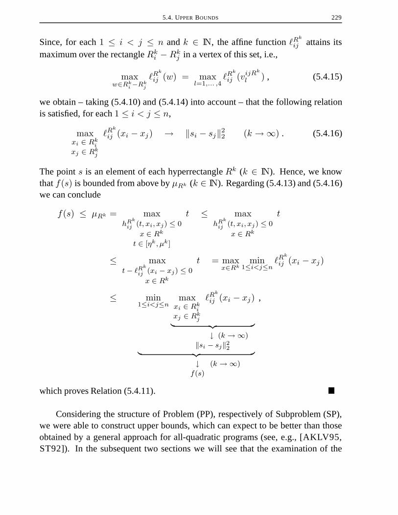
5.4. UPPERBOUNDS 229
Since, for each1 ≤ i < j ≤ n andk ∈ IN, the affine function Rk
ij attains itsmaximum over the rectangleRki − Rkj in a vertex of this set, i.e.,
maxw∈Rk
i−Rk
j
`Rk
ij (w) = maxl=1,... ,4
`Rk
ij (vijRk
l ) , (5.4.15)
we obtain – taking (5.4.10) and (5.4.14) into account – that the following relationis satisfied, for each1 ≤ i < j ≤ n,
maxxi ∈ Rk
i
xj ∈ Rkj
`Rk
ij (xi − xj) → ‖si − sj‖22 (k →∞) . (5.4.16)
The points is an element of each hyperrectangleRk (k ∈ IN). Hence, we knowthatf(s) is bounded from above byµRk (k ∈ IN). Regarding (5.4.13) and (5.4.16)we can conclude
f(s) ≤ µRk = maxhRk
ij (t, xi, xj) ≤ 0
x ∈ Rk
t ∈ [ηk , µk ]
t ≤ maxhRk
ij (t, xi, xj) ≤ 0
x ∈ Rk
t
≤ maxt − `Rk
ij (xi − xj) ≤ 0
x ∈ Rk
t = maxx∈Rk
min1≤i<j≤n
`Rk
ij (xi − xj)
≤ min1≤i<j≤n
maxxi ∈ Rk
i
xj ∈ Rkj
`Rk
ij (xi − xj)
︸ ︷︷ ︸↓ (k → ∞)
‖si − sj‖22︸ ︷︷ ︸
↓ (k → ∞)
f(s)
,
which proves Relation (5.4.11). �
Considering the structure of Problem (PP), respectively of Subproblem (SP),we were able to construct upper bounds, which can expect to be better than thoseobtained by a general approach for all-quadratic programs (see, e.g., [AKLV95,ST92]). In the subsequent two sections we will see that the examination of the

230 PACKING EQUAL CIRCLES IN A SQUARE
structure of (PP) can also be exploited for the subdivision of the current hyperrect-angleRk. Doing this we will be able to substantially reduce the effort for solvingProblem (PP) with Algorithm 5.1. However, we have to keep in mind that thesubdivision set manipulation strategies introduced in Sections 5.5 and 5.6 fulfillCondition (C1) and Condition (C3).
5.5. Subdivision Strategies
LetRk = Rk1 × . . .×Rkn be the current hyperrectangle considered in iterationk ∈ IN of Algorithm 5.1. As pointed out in the description of our approach (seeSection 5.3) we choose in Step II an indexj ∈ {1, . . . , n} such that the rectangleRkj = [lkj1 , L
kj1 ]× [lkj2 , L
kj2 ] has the longest edge-length among all rectangles form-
ingRk. In Step III of Algorithm 5.1 we subdivide this rectangle in order to obtaina subdivision of the hyperrectangleRk. However, until now we did not say how wedo that.
In the present section we describe the strategy applied for splitting the chosenrectangleRkj into a finite number of subrectangles. In order to simplify the pre-sentation we ignore the iteration counterk in the following. We start this sectionwith a description of the basic strategy leading to a partition ofRj . After this wediscuss some special features of our subdivision strategy. Exploiting the structureof Problem (PP) they enable us to avoid redundant computations.
5.5.1. Basic Strategy.If the two-dimensional rectangleRj coincides with theunit squareU , we construct a partition ofRj (see Definition 1.2.1) consisting ofthe four squares
U1 = [0.0, 0.5]× [0.0, 0.5]
U2 = [0.5, 1.0]× [0.0, 0.5]
U3 = [0.0, 0.5]× [0.5, 1.0]
U4 = [0.5, 1.0]× [0.5, 1.0] .
(5.5.1)
(see Figure 5.13(a)). Note that in Algorithm 5.1 the rectangleRj is initializedwith U = [0, 1]2. In the next level, i.e., ifRj is equal to one of the squaresU1, U2, U3 or U4, we obtain a refined partition by constructingm2 squaresUl(l ∈ {1, . . . ,m2}) with equal size and edge-length0.5m . The choice of the integerm with m ≥ 2 depends on the value of the first lower boundη0 > 0 determinedby the first best known solution for (PP) (see the initialization phase of Algorithm5.1). This choice shall assure that the squared diameter ofUl (l ∈ {1, . . . ,m2}) is

5.5. SUBDIVISION STRATEGIES 231
FIGURE 5.13. Basic subdivision strategy
U3
U1 U2
U4
1.0
0.5 1.0
0.5
0.0
(a)Rj = U
0.5
0.5
0.0
<√η0
(b) Rj = U1, m = 3
smaller thanη0 (see Figure 5.13(b)). For that reason we choosem as the solutionof the optimization problem
min m(Lj1−lj1
m
)2
+(Lj2−lj2
m
)2
< η0
m ∈ IN ,m ≥ 2 .
Selectingm in this way we know that at most one memberx?k of an optimal solu-tion (x?1, . . . , x
?n)T ∈ Un of Problem (PP) can belong to one of these squaresUl
(l ∈ {1, . . . ,m2}).REMARK 5.5.1. In our numerical tests it was sufficient to choosem = 2 for
n ≤ 13 andm = 3 for n ≤ 27.
In deeper levels, i.e., ifRj has a maximal edge-length smaller than or equalto 0.5
m , we subdivideRj again into four rectangles with equal size by bisecting theedges of this rectangle.
REMARK 5.5.2. As we will see in Section 5.6, it is possible thatRj shrinksto an interval, i.e., to a one-dimensional rectangle. In these cases we simply splitRj by halving this interval.
The reason for choosing a partition consisting of more than four squares in thesecond level has a heuristical nature. Our numerical tests showed that this strategy– in connection with the following special features and the possible reductions of

232 PACKING EQUAL CIRCLES IN A SQUARE
the size of relevant rectangles discussed in Section 5.6 – has a much better running-time performance than the simpler strategy, whereRj is always divided into foursquares.
For the implementation of the following special features it is essential that atleast in the first level we use squares as partition sets instead of two-dimensionalrectangles with different edge-length, as it is done in [DGPWM91].
5.5.2. Special Features.Because of the special structure of Problem (PP)there are many optimal solutions differing only by the numbering of their mem-bers or differing by a rotation or a reflection.
Consider the casen = 6. An optimal solution of Problem (PP) is given by
x1 =(
00
), x2 =
(1312
), x3 =
(23
0
), x4 =
(112
),
(5.5.2)
x5 =(
01
), x6 =
(23
1
), t = 13
36
(see Figure 5.14(a)). Setting, for eachi ∈ {1, . . . , 5}, xi := xi+1 andx6 := x1
FIGURE 5.14. Same solutions with different numbering
x2
x3
x4
x1
x5 x6
0 1
1
(a) Numbering 1
x1
x2
x3
1
1
0 x6
x4 x5
(b) Numbering 2
we obtain the "same" optimal solution (see Figure 5.14(b)). The membersxi of anoptimal solution are permutable. However, for the solution of the point scatteringproblem it is sufficient if we detect one of thesen! optimal solutions. Hence, weneed a subdivision strategy, which guarantees aunique numbering.

5.5. SUBDIVISION STRATEGIES 233
In order to illustrate the problem of possible rotations and reflections consideragain the casen = 6. There are8 possible symmetric arrangements of an optimalsolution(x1, . . . , xn)T ∈ Un in the unit squareU . For the optimal solution given
FIGURE 5.15. Solutions differing by rotation
x2
x3
x4
x1
x5 x6
0 1
1
(a)0◦ rotation
x5
x2
x1
x3x6
x41
10
(b) 90◦ rotation
x5
x2x4
x3 x1
0 1
1
x6
(c) 180◦ rotation
1
1
x5x1
x4
x3 x6
x2
0
(d) 270◦ rotation
in (5.5.2) (see Figure 5.15(a)), there are three possible rotations (Figures 5.15(b)-5.15(d)) and four reflections (Figures 5.16(a)-5.16(d)). For Algorithm 5.1 it wouldbe sufficient, if only one of these possibilities is considered. Therefore, we needalso a strategy, which avoids that Algorithm 5.1 looks for more than one of thesesymmetric solutions. Note that these reflections and rotations are the results oforthogonal transformations, which do not change the Euclidean distances betweenthe members of a pointx ∈ Un.

234 PACKING EQUAL CIRCLES IN A SQUARE
FIGURE 5.16. Solutions differing by reflection
x1
x4
x6 x5
0 1
1
x3
x2
(a) Reflection along[(
0.50
),(0.51
)]x6x5
x1 x3
0 1
1
x2 x4
(b) Reflection along[(
00.5
),(
10.5
)]
0
1
1
x1x5
x4
x6 x3
x2
(c) Reflection along[(01
),(10
)]
x1
x2
x5
x6x3
x41
0 1
(d) Reflection along[(00
),(11
)]
REMARK 5.5.3. The arrangements displayed in Figure 5.15 and in Figure5.16 differ only by the numbering of the members of the solution(x1, . . . , xn)T
(compare, e.g., Figures 5.15(a) and 5.16(b)). Consequently, one could assume thata unique numberingstrategy also reduces the number of possible symmetric ar-rangements, and it would be thus not necessary to consider all displayed cases ina symmetry avoiding strategy. However, the fact that the reflections lead onlyto a different numbering in comparison with the rotations depends on the specialstructure of the considered solution forn = 6. This solution is symmetric itself. Ifan optimal solution for Problem (PP) is not symmetric, as it is for example the casefor n = 10 (see Figure 5.17), then there exist8 completely different arrangements.

5.5. SUBDIVISION STRATEGIES 235
FIGURE 5.17. A solution of Problem (PP) forn = 10
ad 5.15(a) ad 5.15(b) ad 5.15(c) ad 5.15(d)
ad 5.16(a) ad 5.16(b) ad 5.16(c) ad 5.16(d)
In the following we would like to sketch how we obtain the required uniquenumbering and how we try to avoid the appearance of symmetric solutions. Westress that the elimination of redundant solutions is crucial for the efficiency ofAlgorithm 5.1 (see also Remark 5.6.1 in the next section). The algorithm necessar-ily refines the branch-and-bound tree near all optimal solutions that have not beenidentified as "simple modifications" of each other. Thus the amount of time savedby eliminatingk − 1 of k solutions is nearly a factor ofk.
Unique Numbering. In order to describe the simple idea of this special strat-egy let us assume that a hyperrectangle
R = R1 × · · · ×Rnis given such that, for eachi ∈ {1, . . . , n}, the rectangleRi is subdivided twice,i.e.,Ri is the result of a subdivision of one of the four squaresUi (i = 1, . . . , 4) (see(5.5.1)). Taking the basic strategy into account it follows that, for each rectangleRi (i ∈ {1, . . . , n}), there exists a unique squareUi ⊂ U with edge length0.5
m
satisfyingRi ⊂ Ui. If we identify each of the4m2 possible squaresU with a

236 PACKING EQUAL CIRCLES IN A SQUARE
unique numberno(U) and require that, for anyi = 1, . . . , n− 1, there holds
no(Ui) < no(Ui+1) , (5.5.3)
then we are able to guarantee a unique numbering of the rectangles forming thehyperrectangleR.
Let us illustrate this approach with an example. Consider again the casen = 6and assume thatm is chosen as2. In this situation there are16 possible squaresU . Numbering these possibilities as shown in Figure 5.18 and requiring that (5.5.3)
FIGURE 5.18. Unique numbering
2 5 6
8743
9 10 13 14
1612 1511
1
1
0 1
is true, we see that solutionx displayed in Figure 5.14(b) is not possible. Indeed,x is a member of the hyperrectangleR = R1 × · · · × R6 given in Figure 5.19(b)with the propertyno(U6) < no(U1). This violates Condition (5.5.3). On the other
FIGURE 5.19. Different numberings
��������
��������
������
������
��������
����������������
��������
������������
������������
���������
���������
R3
0 1
1
R5 R6
R4
R1
R2
(a) Possible
��������
��������
��������
��������������������
������������
������������
������������
���������
���������
������
������
0 1
1
R6
R4 R5
R3
R2
R1
(b) Impossible
������
������
��������
��������������������
������������
������������
������������
���������
���������
������
������
R3
0 1
1
R1
R4 R6
R5
R2
(c) Possible
hand, a numbering of solutionx as in Figure 5.14(a) is allowed, since this point iscontained in the hyperrectangleR = R1 × · · · ×R6 shown in Figure 5.19(a).

5.5. SUBDIVISION STRATEGIES 237
As mentioned before, this strategy guarantees a unique numbering of the rect-anglesRi forming the considered hyperrectangleR. Unfortunately, this strategyis not able to ensure a unique numbering of an optimal solution, i.e., Algorithm5.1 using this strategy can still look for several solutions of Problem (PP) differingonly by the numbering of their members. Indeed, with respect to the basic strat-egy we know that each squareU resulting from the second partition ofU containsat most one member of an optimal solution. However, if a member of an optimalsolution belongs to the boundary of such a squareU , this set is not unique, as it isthe case forxi =
(0.330.5
)or xj =
(1.00.5
)in our present example. In such a situation
our strategy does not guarantee a unique numbering of the optimal solution. Thenumbering of the hyperrectangleR = R1×· · ·×R6 given in Figure 5.19(c) fulfillsalso Property (5.5.3). Hence, Algorithm 5.1 – even using this unique numberingstrategy – has to detect an optimal solution in hyperrectangleR (Figure 5.19(a))as well as in hyperrectangleR (Figure 5.19(c)). Nevertheless, this special featurestrongly reduces the necessary effort for solving Problem (PP). Note that we elim-inate till the second partitioning leveln!− 1 of n! possible hyperrectangles.
Symmetry Avoiding Strategy. Let
R = {R = R1 × · · · ×Rn ⊂ U2n,
Ri = [li1 , Li1 ]× [li2 , Li2 ] ⊂ U , i = 1, . . . , n}
be the set of all possible2n-dimensional hyperrectangles. The symmetries result-ing from the relevant rotations and reflections (see again Figure 5.15 and Figure5.16) can be interpreted as an equivalence relation∼ on the setR.
R,Q ∈ R : R ∼ Q ⇐⇒R is the result of one of the three possiblerotations ofQ or the result of one of thefour possible reflections ofQ
The equivalence relation∼ divides R into equivalence classesRι (ι ∈ I,
I index set), i.e.,
• Rι ⊂ R, ∀ι ∈ I• R ∼ Q, ∀R,Q ∈ Rι, ι ∈ I• Rι ∩Rκ = ∅, ∀ι, κ ∈ I, ι 6= κ
• ⋃ι∈I Rι = R .

238 PACKING EQUAL CIRCLES IN A SQUARE
Obviously, it is sufficient for a correct functioning of Algorithm 5.1 if thismethod considers only one member of the equivalence classesRι, which are rele-vant during the execution of our approach. We developed a strategy able to decidewhether a given hyperrectangleR = R1 × · · · × Rn in a node of the branch-and-bound tree is aspecialrepresentative of an equivalence class or not. Let us shortlysketch the basic ideas of this strategy.
Assume at first that we are in a situation such that the current hyperrectangleR is given as the Cartesian product of the squaresUi (i ∈ {1, . . . , 4}) (see (5.5.1)),i.e., each memberRi of R has been subdivided once. If the previously describedunique numbering strategy is applied, then we know that there are three integersi1,i2, i3 ∈ {1, . . . , n+ 1} (i1 ≤ i2 ≤ i3) satisfying
Ri = U1 i = 1, . . . , i1 − 1 ,
Ri = U2 i = i1, . . . , i2 − 1 ,
Ri = U3 i = i2, . . . , i3 − 1and
Ri = U4 i = i3, . . . , n .
Note that the unique numbering strategy can also be applied for hyperrectangleswith this structure, even though we described the ideas of this method under theassumption that each member of the considered hyperrectangle is subdivided twice.Denote by
C1 := i1 − 1 , C2 := i2 − i1 , C3 := i3 − i2 , C4 := n+ 1− i3the number of membersRj (j ∈ {1, . . . , n}) of R, which are equal toUi(i ∈ {1, . . . , 4}). In order to avoid that Algorithm 5.1 considers more than onerepresentative of the equivalence class of the setR containing the hyperrectangleR we require that these countersC1, C2, C3 andC4 fulfill special ordering con-ditions.
Ordering conditions for the first level
C1 ≥ max{C1, C2, C3} (OC1)
C2 ≥ C3 (OC2)
If C1 = C2 ThenC3 ≥ C4 (OC3)
If C1 = C3 ThenC2 ≥ C4 (OC4)

5.5. SUBDIVISION STRATEGIES 239
If a hyperrectangleR = R1 × . . . × Rn does not fulfill (OC1), it is possible torotate the rectangles forming this set such that (OC1) is satisfied. Condition (OC2)can be reached by a reflection along the line
[(00
),(11
)]and Condition (OC3) is
yielded by a reflection along[(
0.50
),(0.51
)]. If Condition (OC4) is not satisfied we
can reflect the members ofR along the line[(
00.5
),(
10.5
)]and obtain an element of
the same equivalence class fulfilling this condition. Note that all Conditions (OC1)-(OC4) are satisfiable simultaneously. The examination of the reflection along theline
[(10
),(01
)]in the first level does not lead to another ordering condition. We
could only requireC1 ≥ C4. However, this is fulfilled regarding Condition (OC1)and thus unnecessary.
Let us illustrate these conditions for the casen = 6. As mentioned before, wewould like to avoid that Algorithm 5.1 tries to determine the solutions displayedin Figures 5.15(b)-5.15(d). In order to detect these solutions Algorithm 5.1 has togenerate the hyperrectangles
R1 = U1 × U1 × U2 × U2 × U3 × U4 ,
R2 = U1 × U2 × U2 × U3 × U4 × U4 ,
R3 = U1 × U2 × U3 × U3 × U4 × U4 ,
R4 = U1 × U1 × U2 × U3 × U3 × U4 ,
R5 = U1 × U2 × U2 × U3 × U3 × U4
and
R6 = U1 × U1 × U2 × U3 × U4 × U4 .
(see Figure 5.20). Only the hyperrectanglesR1 andR6 satisfy (OC1)-(OC4) si-multaneously. Indeed,R2,R3 andR5 violate (OC1) andR4 does not fulfill (OC2).Hence, Algorithm 5.1 eliminates these four sets from further considerations. Thismeans that only one-third of the hyperrectangles containing optimal solutions haveto be analyzed further. However, because of the special structure of the solutionfor n = 6 – x2 andx4 does not belong to a unique squareUi (i ∈ {1, . . . , 4}) –the remaining hyperrectanglesR1 andR6 still contain the four possible symmetricarrangements ofx. The solutions given in Figures 5.15(a) and 5.15(c) lie inR1
and all solutions are located withinR6. For that reason we have to examine thesymmetry structure of the relevant hyperrectangles also in the second level.
Assume now that the current hyperrectangleR is given by the Cartesian prod-uct of n rectangles with edge-length0.5m , i.e., each member ofR is subdivided

240 PACKING EQUAL CIRCLES IN A SQUARE
FIGURE 5.20. Hyperrectangles containing an optimal solution
0 1
1
C1 = 2 C2 = 2
C3 = 1 C4 = 1
(a)R1
0 1
1
C1 = 1
C3 = 1 C4 = 2
C2 = 2
(b) R2
0 1
1
C1 = 1
C3 = 2 C4 = 2
C2 = 1
(c) R3
0 1
1
C1 = 2
C3 = 2 C4 = 1
C2 = 1
(d) R4
0 1
1
C1 = 1
C3 = 2 C4 = 1
C2 = 2
(e) R5
0 1
1
C1 = 2
C3 = 1 C4 = 2
C2 = 1
(f) R6
twice. According to the choice ofm we know that each rectangleRi(i ∈ {1, . . . , n}) formingR contains at most one member of an optimal solutionof Problem (PP) and hence the rectanglesRi (i ∈ {1, . . . , n} must be differentfrom each other. Moreover, we know thatR is a child of a hyperrectangleR, whichhas satisfied all conditions in the first level and we know which type of symmetryare still possible, i.e., with respect to which type of symmetry isR invariant. Forexample, in the casen = 6 there holds that forR1 and hence for all its childrenonly the reflection along the line
[(0.50
),(0.51
)]can be considered. The other pos-
sible hyperrectangleR6 is invariant with respect to180◦ rotations as well as withrespect to reflections along
[(00
),(11
)]and along
[(01
),(10
)].
In order to avoid that Algorithm 5.1 examines more than one representative ofthe equivalence classes containing hyperrectangles with the described structure weassign to each squareUi (i ∈ {1, . . . , 4}) a number, as we did in the first level.However, this number is not a pure integer anymore. We use binary representationsof integer values with a length ofm2. An element of them2-dimensional binary

5.5. SUBDIVISION STRATEGIES 241
vector corresponds to one of them2 possible subsquares obtained by partitioningUi (i ∈ {1, . . . , 4}) according to the basic strategy. Such an element is set to1,if the corresponding square is a member ofR, and0 otherwise. Consider the casem = 2. We have4 possible subsquares of edge-length0.25 for each squareUi(i ∈ {1, . . . , 4}). In order to examine rotation symmetries we define the vectorsC1, C2, C3, C4 ∈ {0, 1}4 as shown in Figure 5.21. As in the first level we require
FIGURE 5.21. Numbering ofC1, C2, C3, C4 for rotation sym-metries andm = 2
0
1
1
C32
C13
C11 C12
C14
C34 C44
C24
C21
C22
C43
C23
C31 C33 C42 C41
that the integers given by the binary vectorsC1, C2, C3 andC4 fulfill special or-dering conditions – likeC1 ≥ max{C2, C3, C4} (compare with Condition (OC1)for the first level). Note that the numbering of the vectors is chosen such that theyare invariant with respect to the rotations. The same has to be done, if we examinepossible reflections. In these cases we choose form = 2 the numberings givenin Figures 5.22(a)-5.22(d). The resulting integers are also checked, whether theyfulfill special ordering conditions.
It is essential to note that in the cases where more than one type of symmetrycan be examined we have to pay attention that the applied conditions are consistent.Recognize that in contrast to the first level the integers used here for checking theordering conditions can vary for different symmetries. This means that we have toguarantee that all conditions, which we require, can be fulfilled simultaneously byat least one element of each relevant equivalence class ofR. This problem leads toa distinction of many cases in order to formulate these conditions. Therefore, weabandon an explicit formulation of the used conditions in the present work.

242 PACKING EQUAL CIRCLES IN A SQUARE
FIGURE 5.22. Numbering ofC1, C2, C3, C4 for reflectionsymmetries andm = 2
1
0 1
C32
C13
C11 C12
C14
C34 C44
C24
C21
C23
C42
C22
C31 C33 C43 C41
(a) along[(
0.50
),(0.51
)]0
1
1
C33
C13
C11 C12
C14
C34 C44
C24
C21
C22
C42
C31 C32 C41
C23
C43
(b) along[(
00.5
),(
10.5
)]
0
C13
C11 C12
C14
C44 C42
C43 C41
1
1
(c) along[(
01
),(10
)]
1
1
C33 C34
C24
C21
C22
C23
C31 C32
0
(d) along[(
00
),(11
)]
REMARK 5.5.4.
(a) If m is different from2, as it is the case for numerically interesting num-bers of points (see Remark 5.5.1), we have to adjust the numbering of them2-dimensional binary vectorsC1,C2,C3 andC4 according to the previ-ous ideas. Moreover, theconsistentordering conditions, which we requireto be fulfilled, have also to be adapted in these cases.

5.5. SUBDIVISION STRATEGIES 243
(b) If the considered hyperrectangle is a child of a set invariant with respect toreflections along the line
[(10
),(01
)]or along
[(00
),(11
)], it is also possible to
formulate additional conditions considering the subsquares ofU2 andU3 orof U1 andU4, respectively, which are not crossed by the reflection line (seethe not-numbered subsquares in Figure 5.22(c) or in Figure 5.22(d)).
Let us finally illustrate the described symmetry avoiding strategy in the secondlevel for our examplen = 6. The hyperrectanglesR11 andR12 given in Figure5.23 are children ofR1 and hence possible during the execution of Algorithm 5.1.
FIGURE 5.23. Possible children ofR1 for n = 6
��������
��������
������
������
��������
��������
������������
������������
���������
���������
��������
��������
0 1
1
(a)R11
��������
��������
������������
������������������������
������������
��������
��������
������
������
���������
���������
0 1
1
(b) R12
As we have pointed out before, the hyperrectangleR1 is only invariant with re-spect to reflections along the line
[(0.50
),(0.51
)]. According to the numbering of the
4-dimensional binary vectors given in Figure 5.22(a) we obtain:
R11:
C1 = (1, 0, 0, 1)T
C2 = (0, 1, 1, 0)T
C3 = (1, 0, 0, 0)T
C4 = (0, 0, 1, 0)T
R12:
C1 = (0, 1, 1, 0)T
C2 = (1, 0, 0, 1)T
C3 = (0, 0, 1, 0)T
C4 = (1, 0, 0, 0)T
If we use the condition
C1 ≥ C2 ,
we see thatR11 satisfies this condition andR12 violates it. HenceR12 is eliminatedfrom further considerations and we obtain that the optimal solution given in Figure

244 PACKING EQUAL CIRCLES IN A SQUARE
5.15(c), which was still contained inR1, is with respect to the children of thishyperrectangle no longer possible.
The hyperrectangleR6 , which fulfills also the ordering conditions in the firstlevel, can lead to the four hyperrectangles given in Figure 5.24 containing the four
FIGURE 5.24. Possible children ofR6 for n = 6
����
���
���
��������
��������
����
���
���
0 1
1
(a)R61
���
���
��������
����
���
���
���
���
����
0 1
1
(b) R62
����
����
������
������
����
������
����������
0 1
1
(c) R63
����
������
������������
����������
��������
���
���
0 1
1
(d) R64
possible arrangements of the optimal solutions shown in Figure 5.15. We knowthatR6 is invariant with respect to180◦ rotations. Using the numbering of thebinary vectorsC1, C2, C3 andC4 given in Figure 5.21 and requiringC1 ≥ C4– as we did in the first level – we obtain thatR63 andR64 violates this condition.If we consider the reflection along the line
[(00
),(11
)]and require againC2 ≥ C3
(compare with (OC2)), whereC2 andC3 are now numbered as in Figure 5.22(d), itfollows thatR61 does not fulfill this condition. Thus using our ordering conditions,only the hyperrectangleR62 remains.
Applying the described symmetry avoiding strategy in the second level it fol-lows again that two-third of the hyperrectangles containing symmetric solutions areeliminated from further considerations. Unfortunately, there are still two symmet-ric solutions (see Figure 5.15(a) and Figure 5.15(b)), which have to be detected byAlgorithm 5.1, sinceR11 andR62 fulfill all ordering conditions and contain botharrangements ofx. The reason for this fact is again the special structure of thesolutionx for n = 6 given in (5.5.2). As in the first level, there are two differentequivalence classes ofR, whose members contain symmetric arrangements ofx.
Hence our symmetry avoiding strategy is not able to fully avoid that Algorithm5.1 has to detect different symmetric solutions. We can only guarantee that Algo-rithm 5.1 does not look for optimal solutions in more than one representative of anequivalence class ofR. This is the best we can obtain and – as it was the case for

5.5. SUBDIVISION STRATEGIES 245
the unique numbering strategy – we have seen in our example that the use of thesuggested symmetry avoiding strategy reduces significantly the effort for solvingProblem (PP) with Algorithm 5.1.
If a hyperrectangleR fulfilling all required conditions in the second level isstill invariant with respect to some types of symmetry, we could examine thesesymmetries also in deeper levels. However, our numerical experience showed thatthis effort does not lead to an improvement of the numerical performance of Algo-rithm 5.1 – at least as long as the size reduction strategies introduced in the nextsection are used.
Besides these two special features, which do not depend on the current upperand lower bounds, we also use a third idea in order to reduce the effort for solv-ing Problem (PP). This idea exploits explicitly the knowledge of the current bestknown valueη.
Using the Current Lower Bound η. If we assume that for the cases2 ≤ l < n
upper boundsµ(l) for the optimal solution valuet?(l) are known, then it is possibleto further reduce the number of subdivision setsR = R1 × · · · × Rn, which arerelevant during the execution of Algorithm 5.1. Note that the presented approachcan deliver the necessary upper boundsµ(l).
For a given hyperrectangleR = R1 × · · · ×Rn ⊂ U2n and for2 ≤ l < n, let
Rl = {{Ri : i ∈ I} with I ⊂ {1, . . . , n}, |I| = l}be the set of all subsets of{Ri, i = 1, . . . , n} with cardinalityl. Choose, forl < n,a setQ ∈ Rl and let
Q = [l1, L1]× [l2, L2]
be the smallest rectangle containing all elements ofQ. Since there holdsµ(l) ≥t?(l) it is obvious that the maximal minimum pairwise squared distance ofl pointslying inside a square with edge lengthd is not greater thanµ(l)d2.
If there holds
µ(l)(max{L1 − l1, L2 − l2})2 < η , (5.5.4)
it is not possible thatl points lie insideQ with a minimum squared distance biggerthan or equal toη. Thus it is not necessary to considerR further, sinceR cannotcontain a pointx ∈ IR2n with a better distance behavior than the current best knownpoint.

246 PACKING EQUAL CIRCLES IN A SQUARE
Let us illustrate this method with an example. Consider again the casen = 6and assume that the current rectangleR = R1 × · · · × R6 has the structure givenin Figure 5.25. We know thatµ(4) = 1 = t?(4). Hence we can derive that the
FIGURE 5.25. Eliminable case
���������
���������������������
������������
������������
��������������
����
������
���������
���������
������
������
R4
R1
R3
R6 QR5
R2
10
1
maximal minimum pairwise squared distance of four points lying inside the square
Q = [0.5, 1.0]× [0.25, 0.75] = R2 ∪R3 ∪R5 ∪R6
is equal to0.25 = µ(4)0.52. If a current best known valueη greater than0.25 isgiven, we are able to eliminateR from the set of relevant hyperrectangles withoutlosing an optimal solution of Problem (PP).
REMARK 5.5.5.
(a) In Algorithm 5.1 (see Section 5.3) we use the subdivision strategies de-scribed so far in the following way. At first we partition the current rec-tangleRj in 4 orm2 rectanglesR1
j , · · · , Rlj (l ∈ {4,m2}) with equal sizefollowing the basic strategy. After this we use the special features in order totest whether it is possible to eliminate some of the resulting hyperrectangles
Ri = R1 × · · · ×Rj−1 ×Rij ×Rj+1 × · · · ×Rn , i = 1, . . . , l .
In this way we obtainl (0 ≤ l ≤ l) hyperrectangles, which have to beanalyzed further.
(b) Note that in the execution of Algorithm 5.1 it is not necessary that all two-dimensional rectangles forming the hyperrectangleR have equal size, sincewe split in each iteration only one partRj . For simplicity of presentation wehave assumed in the description of the subdivision strategies in the presentsection that all rectanglesR1, . . . , Rn forming the current hyperrectangle

5.6. SIZE REDUCTION STRATEGIES 247
have equal size (compare with the previous figures). In the implementa-tion of Algorithm 5.1 we took the possibility of different sizes into account.It is possible to adapt all subdivision strategies mentioned before to theexamination of hyperrectangles consisting of members without equal size.However, doing this we have to pay attention to the fact that the strategiesused in our algorithm can interfere with each other. For instance, the con-ditions for the symmetry avoiding strategies have to recognize the uniquenumbering strategy. Therefore, we have to ensure that all conditions, whichwe require to be satisfied, work simultaneously.
In the description of Algorithm 5.1 in Section 5.3 we postulate that the subdivi-sion strategies fulfill Conditions (C1) and (C3). Since our basic strategy generatesmore and smaller subsets ofR than the bisection strategy would do, it follows im-mediately that our subdivision strategy is exhaustive, i.e., satisfies (C1). Note thatthe bisection of hyperrectangles is exhaustive.
In the discussion of the special features we have seen that we lose optimalsolutions applying our strategies. Nevertheless, it is possible to implement thesestrategies such that we never lose all solutions. Therefore, our subdivision strate-gies are also consistent in the sense of Condition (C3).
The described special features reduce the effort for solving Problem (PP) byavoiding possible, but redundant partition sets in advance. Only the last idea takesadvantage of the information generated by the algorithm itself. Exploiting theseinformation in a stronger way it is possible to reduce the size of the hyperrectangles,which are not eliminated from consideration by these subdivision strategies. Howwe realize this is the content of the next section.
5.6. Size Reduction Strategies
LetR = R1×. . .×Rn ⊂ IR2n be a hyperrectangle in an iteration of Algorithm5.1 withRi = [li1 , Li1 ]× [li2 , Li2 ] ⊂ U (i ∈ {1, . . . , n}), and letη > 0 andµ ≤ 2respectively be the current lower and upper bound. Assume that this hyperrectanglebelongs to the sets remaining after the execution of the subdivision strategies inStep III. Note that we ignore the iteration indexki (i ∈ {1, . . . , l}, k ∈ IN) in orderto reduce the number of necessary indices, as we did in the previous section.
In the formulation of Algorithm 5.1 (see, especially, Step IV) we claimed thatis can be possible to diminish the size of the hyperrectangleR. In the present

248 PACKING EQUAL CIRCLES IN A SQUARE
section we describe the strategy, which can lead to such a reduction of the size ofthe setR.
In the derivation of the theoretical results in Section 5.2 we saw that for Prob-lem (PP) there always exist optimal solutions satisfying special properties. In par-ticular, we know that there is an optimal solutionx? = (x?1, . . . , x
?n)T ∈ Un with
optimal valuet?(n) fulfilling the properties
(P3): either a vertexv of the unit squareU is a member ofx? itself, or thereexist two members ofx? lying on the edge-lines ofU forming the vertexv, which have exactly the optimal distance (Theorem 5.2.3 and Corollary5.2.4), and
(P4): two consecutive members ofx? belonging to the same edge ofU havea distance smaller than two times the optimal one (Theorem 5.2.6).
It is sufficient, if Algorithm 5.1 looks only for optimal solutions satisfyingthese properties. This means that we can interpret each pointx ∈ Un, whichdoes not have these attributes, as an infeasible point for (PP). Doing this we canfurther reduce the number of possible optimal solutions of Problem (PP), as it wasthe case by applying the special features of the subdivision strategy developed inthe previous section. Indeed, consider the casen = 7. One optimal solution isdisplayed in Figure 5.26(a). The pointx7 is not unique. We can choose each point
FIGURE 5.26. Solutions forn = 7
����
x2
x1
x6x4
t?(7)
10
1x5
x3
x7
(a)
x2
x1
x6x4
10
1x5
x3
x7
(b)
in the shaded region without changing the minimum pairwise distance. However,only the solution shown in Figure 5.26(b) fulfills Property (P3).
5.6. SIZE REDUCTION STRATEGIES 249
REMARK 5.6.1. Global optimization approaches, in particular branch-and-bound methods, generally have problems if many global optimal solutions exist.For example, branch-and-bound methods often have to strongly refine the subdivi-sion sets in a neighborhood of an optimal solution in order to reduce the distancebetween the upper and lower bounds until the required tolerance is reached. There-fore, it is not surprising that the effort for solving a problem increases significantlyif the number of global optimal solutions grows. On the other hand, we are satis-fied if the solution method detects oneglobal solution. Consequently, each strategyreducing the number of possible solutions of a problem can improve the numericalperformance of a global optimization approach. However, such strategies cannotbe derived in general. Nevertheless, exploiting the structure of special problem in-stances we can expect to obtain suchsolution elimination strategies. Note that theunique numbering strategy as well as the symmetry avoiding strategy introduced inthe previous section and the strategies enforcing the satisfaction of Property (P3)and of Property (P4) discussed in the sequel can be interpreted as such solutionelimination strategies.
In the subsequent two subsections we will see, how it is possible to enforce thata solution of Problem (PP) detected by Algorithm 5.1 has the required attributesand how this enforcement leads to a reduction of the size ofR. Using Property(P3) we derive the so-calledcorner rules, which can result in a shrinkage of somerectanglesRi (i ∈ {1, . . . , n}) – forming the hyperrectangleR – to an interval oreven to a single point. Exploiting Property (P4) we obtain the so-callededge rules.In Subsection 5.6.2 we will see that the application of these rules can also reducesome rectangles to intervals. Hence the enforcement of Properties (P3) and (P4)lead to a reduction of the size ofR through a reduction of the dimension of this set.
We complete the size reduction strategies with a third strategy reducing thevolume of the hyperrectangleR. This strategy does not base on the properties ofan optimal solution mentioned above. As the last special feature of our subdivisionstrategies, it uses the knowledge of the current best known valueη. We will see thatthe use of this knowledge enables us to eliminate parts ofR, which cannot containa pointx ∈ Un with a larger minimum pairwise distance than the best known sofar.
5.6.1. Corner Rules. If we analyze the behavior of the given subdivision setR = R1 × . . .×Rn in the neighborhood
S(v, µ) = {x ∈ U : ‖x− v‖22 ≤ µ}

250 PACKING EQUAL CIRCLES IN A SQUARE
of the vertexv of the unit squareU , then we recognize that there exist some situa-tions allowing us to reduce the dimension of selected rectanglesRi(i ∈ {1, . . . , n}). Remember thatµ is an upper bound for the optimal valuet?(n)of Problem (PP).
Indeed, letv ∈ IR2 be an arbitrary vertex of the unit squareU and denote bye1 ande2 the edge-lines ofU forming this vertex, i.e., fori ∈ {1, 2}, there holdsei = {x ∈ U : xi = vi}. Denote now by
S(v, µ) = {Ri : i ∈ {1, . . . , n} with Ri ∩ S(v, µ) 6= ∅and∃l ∈ {1, 2} satisfyingRi ∩ el 6= ∅}
the set of all two-dimensional rectanglesRi (i ∈ {1, . . . , n}) forming the hyper-rectangleR, which have a non-empty intersection withS(v, µ) and which, addi-tionally, touch the edge-linee1 or the edge-linee2 or both. Depending on the car-dinality of S(v, µ) we distinguish four cases (compareS(v, µ) with S(v, t) used inthe proof of Theorem 5.2.3 in Section 5.2).
Case 1: |S(v, µ)| = 0
Sinceµ is an upper bound for the optimal solutiont?(n) of Problem (PP), it followsimmediately that there does not exist a pointx ∈ R fulfilling Property (P3) at ver-tex v. Hence, it is not necessary to analyzeR further, i.e.,R can be pruned. Notethat we interpret each pointx ∈ Un without Properties (P3) and (P4) as infeasible,and with respect to this interpretation we know that in this caseR contains onlyinfeasible points.
Case 2: |S(v, µ)| = 1
Assume, without loss of generality, that there holdsS(v, µ) = {R1}. If v /∈ R1
(see Figure 5.27(a)), it follows by the same argumentation as in Case 1 thatR iseliminable. Otherwise (see Figure 5.27(b)) we know that only pointsx = (x1, . . . , xn)T ∈ R with x1 = v fulfill Property (P3). Note that (P3b) isnot satisfiable in this case. Thus, we do not lose all optimal solutions of Problem(PP), if we set
R = R1 ×R2 × . . .×Rnwith
R1 = {v} = [v1, v1]× [v2, v2] ,
i.e., if we shrinkR1 to a single point.

5.6. SIZE REDUCTION STRATEGIES 251
FIGURE 5.27. Corner rules (Case 2)
õ
v
e2
U
e1Ri
Rj
R1
(a) Eliminable case
õ
v
e2
U
e1
Rj
Ri
R1
(b) Adjustable case
Case 3: |S(v, µ)| = 2
Assume again, without loss of generality, thatS(v, µ) is equal to{R1, R2}. De-pending on the location ofv with respect toR1 andR2 we have to distinguish twofurther subcases.
Case 3.1: v /∈ R1 ∪R2
It is clear that at vertexv Property (P3a) cannot be satisfied by an elementx of R. If R1 andR2 touch the same edge-lineei (i ∈ {1, 2}) (see Figure5.28(a)), we are able to eliminateR, since in this situation (P3b) is also notpossible. Otherwise (see Figure 5.28(b)) we are able to replaceR1 andR2
by intervals. Setting
R1 := R1 ∩ (e1 ∪ e2)and
R2 := R2 ∩ (e1 ∪ e2)we do not lose any pointx ∈ R fulfilling Property (P3b). Note thatR1
andR2 touches eithere1 or e2, but not both.
Case 3.2: v ∈ R1 ∪R2
In this case it is possible that there exist pointsx ∈ R fulfilling (P3a) andpointsx ∈ R such that (P3b) is true at vertexv. In general there is noway to reduce the dimension of both rectanglesR1 andR2, as we did in the

252 PACKING EQUAL CIRCLES IN A SQUARE
FIGURE 5.28. Corner rules (Case 3.1)
v
U
e2
e1R2R1
Ri
õ
(a) Eliminable case
v
R1Ri
U
e2
R2R2
õ
e1
R1
(b) Adjustable case
previous subcase. However, ifv belongs to one and only one of the rectan-glesR1 orR2 (see Figure 5.29), we can shrink the rectangle containingv
to an interval. Assume that there holdsv ∈ R1 \ R2 (see Figure 5.29(a)).The hyperrectangleR1 ×R2 × . . .×Rn with
R1 :={R1 ∩ e1 , if R2 ∩ e1 = ∅R1 ∩ e2 , if R2 ∩ e2 = ∅
contains any pointx ∈ R satisfying (P3) at vertexv.
FIGURE 5.29. Corner rules (Case 3.2)
R1
e2
U
Ri
R1v
R2 e1õ
(a) Adjustable case
√ηv
R1
R2
R2
Ri
U
e2
e1
R1
(b) Adjustable case

5.6. SIZE REDUCTION STRATEGIES 253
If there holds, additionally,R2 ⊂ {x ∈ U : ‖x−v‖22 < η} (see Figure5.29(b)), we can also reduceR2 to an intervalR2 by intersectingR2 withthe touched edge-linee1 or e2. Note that in this situation it is not possiblethat v is a member of an optimal solutionx belonging toR. Thus, onlyProperty (P3b) can be satisfied.
Case 4: |S(v, µ)| ≥ 3
If one and only one of the rectanglesRi belonging toS(v, µ) touchese1 or e2, weare in a comparable situation as in Case 3.2. We are able to shrink this rectangleto an intervalRi (see Figures 5.30(a) and 5.30(b)). In situations where at least tworectangles touch each edge-linee1 ande2 (see Figures 5.30(c) and 5.30(d)), we
FIGURE 5.30. Corner rules (Case 4)
Ri
RkRi Rj
e2
U
õ
e1v
(a) Adjustable case
Ri
Ri
e2
U
Rj Rkõ
e1v
(b) Adjustable case
vRk Rl
RjRi
U
e2
õ
e1
(c) Not adjustable case
vRk Rl
Rj
Ri
e2
U
e1õ
(d) Not adjustable case

254 PACKING EQUAL CIRCLES IN A SQUARE
do not reduce the dimension of a rectangleRi ∈ S(v, µ). If v does not belongto the hyperrectangleR, as it is shown in Figure 5.30(d), only Property (P3b) canbe fulfilled. Therefore, it could be possible to shrink some rectangles to intervals.Since it is not immediately clear which one we have to choose, we decided to donothing in such a situation. Our numerical experience showed, moreover, that thissituation almost never occurs.
5.6.2. Edge Rules.We are interested in optimal solutionsx? = (x?1, . . . , x?n)T
satisfying (P3) and (P4). For such points it is obvious that there does not exist a seg-ment of a boundary line ofU with length greater than or equal to2√µ ≥ 2
√t?(n), which does not contain a memberx?k (k ∈ {1, . . . , n}) of
x?. Using this fact we are able to reduce the dimension of more rectanglesRi(i ∈ {1, . . . , n}) formingR than by using the previously described corner rulesalone.
In order to explain the strategy applied in our approach lete be an arbitraryboundary line ofU , i.e.,
e ∈ {eji : i ∈ {1, 2} , j ∈ {0, 1}}with eji = {x ∈ U : xi = j}. Furthermore let, for two different pointsv, w ∈ e,e(µ) = [v, w] be a line segment ofe and assume that this segment has a length of2√µ, i.e.,‖v − w‖22 = 4µ. Denote by
L(e, µ) = {Ri : i ∈ {1, . . . , n} andRi ∩ e(µ) 6= ∅}the set of all rectanglesRi (i ∈ {1, . . . , n}) touchinge(µ).
• If there holdsL(e, µ) = ∅, it follows thatR contains no point fulfillingProperty (P4). Hence, as in Case 1 in Subsection 5.6.1, it is not necessary to analyzeR further, i.e.,R can be pruned.• In the cases where more than one rectangleRi (i ∈ {1, . . . , n}) touches
e(µ), i.e.,L(e, µ) > 1 (see Figure 5.31(a)), it is not possible to reduce the size of arectangleRi ∈ L(e, µ) without running the risk of losing all optimal solutions.• If there holds
|L(e, µ)| = 1 ,
we can shrink the unique rectangleRi0 touchinge(µ), i.e.,Ri0 ∩ e(µ) 6= ∅, to aninterval (see Figure 5.31(b)). Indeed, as mentioned before, we know that any point

5.6. SIZE REDUCTION STRATEGIES 255
FIGURE 5.31. Edge rules
2õ
U
Ri Rj
wve
(a) Not adjustable case
2õ
U
Ri0Ri0 Rj
wve
(b) Adjustable case
x ∈ R fulfilling (P3) and (P4) has to satisfy the relation
xi0 ∈ Ri0 ∩ e(µ) .
Therefore, any elementx of the hyperrectangleR, which we are interested in, be-longs also to the setR1 × . . .×Ri0−1 × Ri0 ×Ri0+1 × . . .×Rn with
Ri0 := Ri0 ∩ e(µ) .
These edge rules leads to a change ofR only if L(e, µ) contains less than2elements. With respect to the basic subdivision strategy it is hence not surprisingthat the edge rules can be applied more rarely than the corner rules. Nevertheless,this strategy improves the numerical performance of Algorithm 5.1. Note that theedge rules are not relevant as long as the current upper boundµ is not smaller than0.25.
The corner as well as the edge rules use the current upper boundµ in con-nection with Property (P3) and Property (P4) in order to diminish the size of theconsidered hyperrectangleR via a reduction of its dimension. In the next subsec-tion we will see how it is possible to further reduce the size ofR by exploiting theknowledge of the best known valueη, i.e., of the current lower bound.
5.6.3. Volume Reduction.The third size reduction strategy used in Step IVof Algorithm 5.1 is similar to an approach presented in [DGPWM91]. In contrastto the corner and the edge rules we do not diminish the size of the current hyper-rectangleR by reducing the dimension of some rectanglesRi (i ∈ {1, . . . , n})formingR. In this method we reduce the volume of several rectanglesRi by con-structing smaller rectanglesRi ⊂ Ri still containing all feasible points of Subprob-lem (SP) considered in Step V of Algorithm 5.1, i.e., we design rectanglesRi ⊂ U

256 PACKING EQUAL CIRCLES IN A SQUARE
(i ∈ {1, . . . , n}) with the properties
Ri ⊂ Ri i = 1, . . . , n (5.6.1.a)and
F ⊂ [η, µ]× R1 × . . .× Rn (5.6.1.b)
whereF = {(t, x) ∈ [η, µ]×R1× . . .×Rn : t−‖xi−xj‖22 ≤ 0, 1 ≤ i < j ≤ n}denotes the feasible region of (SP).
We compare the rectanglesRi (i ∈ {1, . . . , n}) pairwise and try to cut away apart of the infeasible areas ofRi while preserving the structure of a rectangle. Theinfeasible area ofRi with respect toF is characterized by the fact that, for eachelementxi of such an area, there does exist an indexj ∈ {1, . . . , n} \ {i} suchthat each element ofRj has a squared distance toxi smaller thanη. In order toexplain our volume reduction strategy in a general way let, fori, j ∈ {1, . . . , n}with i 6= j, two polytopesP ⊂ Ri andQ ⊂ Rj be given by their vertex sets, i.e.,
P = [v1, . . . , vmP ] ,
Q = [w1, . . . , wmQ ] .
Assume that the vertex lists ofP andQ are ordered in such a way thatvi+1 andwi+1 is a direct neighbor ofvi andwi, respectively (see Figure 5.32). Assume
FIGURE 5.32. Vertex numbering ofP
v5
v4
v3
P
v2
v6
v1
further thatP×Q is a superset of the projection ofF onRi×Rj. We are interestedin the set
F := {(x, y) ∈ P ×Q : ‖x− y‖22 ≥ η} ,
since the projection ofF onRi ×Rj is a subset ofF . Denote by
C := ( P ∩ {x ∈ IR2 : max{‖x− y‖22 : y ∈ Q}︸ ︷︷ ︸=max{‖x−wi‖2
2:i=1,... ,mQ}=:fQ(x)
< η )

5.6. SIZE REDUCTION STRATEGIES 257
the set of all pointsx ∈ P with a maximal squared distance to each point inQsmaller thanη, i.e.,C is part of the infeasible area ofP mentioned above. Obvi-ously, there holds
F ⊂ (P \ C)×Q .
This means that we can cut awayC fromP without eliminating a feasible point of(SP). C is a convex set. IfC is not empty, then we do not know whetherP \ Cis still a polytope. However, we would like to preserve the linear structure ofP .Therefore, we look for the smallest polytopeP satisfying
P \ C ⊂ P ⊂ P .
In the sequel we describe the construction of this polytopeP . Assume thatCis not empty and denote by
Cv := {v1, . . . vmP } ∩ Cthe set of all vertices ofP belonging toC. Depending on the structure ofCv wedistinguish three cases.
• If there holdsCv = ∅, it follows that we have to takeP for P itself (seeFigure 5.33), i.e., if no vertexv of P has a maximum squared distance to all vertices
FIGURE 5.33. P = P
������������
������������
Q
Pv4
√η C
w2
w3
v2v3
v5v1
√η
v6
w1
w4
ofQ smaller thanη, then we are not able to reduce the size ofP without losing theconvexity ofP .

258 PACKING EQUAL CIRCLES IN A SQUARE
• If there holdsCv = {v1, . . . , vmP }, it follows immediatelyP \ C = ∅ andwe can eliminateR. Note that in this situation the feasible regionF of Subproblem(SP) is empty.• If Cv is a non-empty real subset of{v1, . . . , vmP }, we can adjustP in the
following way. Assume that there exists an indexr ∈ {1, . . . ,mP − 1} with
Cv = {v1, . . . , vr} , (5.6.2)
i.e., all verticesv of P satisfyingfQ(v) < η are neighboring. Since, for eachj ∈ {1, . . . , r}, there holds
fQ(vj) = max{‖vj − wi‖22 : i = 1, . . . ,mQ} < η ,
it follows that there exist a unique pointv1 on the facet ofP defined by the neigh-boring verticesvmP andv1 with a maximal squared distance to the polytopeQ
equal toη, i.e.,fQ(v1) = η. Note that by construction there holdsfQ(v1) < η andfQ(vmP ) ≥ η. Let vr be the corresponding point with respect to the facet definedby vr andvr+1 (see Figure 5.34(a)). The functionfQ is a maximum of convex
FIGURE 5.34. P 6= P
���������������������������������
���������������������������������
w3
v5vr
v6
v4
CP
Q
w4v3
v1
v2
v1
w2
w1
√η√
η
(a)
��������������������������������������������
��������������������������������������������
w3
v5vr
v6
v4
PQ
w4v3
v1
v2
v1
w2
w1
(b)
functions and hence convex itself. It follows that, for anyx ∈ [v1, v1, . . . , vr, vr],there holds
fQ(x) ≤ η

5.6. SIZE REDUCTION STRATEGIES 259
and thus[v1, v1, . . . , vr, vr] ⊂ clC .
P is a two-dimensional polytope and, therefore, we obtain
P \ C ⊂ P := [v1, vr, vr+1, . . . , vmP ] 6= P
(compare Figure 5.34(b)). If Assumption (5.6.2) is not fulfilled, we adjustP inthe same way by analyzing each subset ofCv consisting of a sequence of directneighboring vertices.
With this general framework we are now able to describe the volume reductionstrategy in a more detailed manner. We use the following iterative process.
INITIALIZATION
Set, fori ∈ {1, . . . , n}, Pi ← Ri, i.e.,
Pi =[(li1li2
),( li1Li2
),(Li1li2
),(Li1Li2
)]LOOP
For i = 1 To n DoFor j = 1 To n Do
If j 6= i ThenComparePi andPj and constructPi in the described way.
Pi ← Pi
If Pi = ∅ Then STOP(F is empty)
EndIfEndFor
EndFor
After the execution of this process we know either thatF is empty, i.e., we caneliminateR from further considerations, or we obtainn two-dimensional polytopesPi given by the list of their vertices. In this situation it is easy to generate, for eachindexi ∈ {1, . . . , n}, the smallest rectangleRi containing the polytopePi. Setting
R := R1 × . . .× Rnwe obtain a hyperrectangleR, which is a subset ofR and, additionally, has theproperty
F ⊂ [η, µ]× R

260 PACKING EQUAL CIRCLES IN A SQUARE
(compare with the required Properties (5.6.1.a) and (5.6.1.b)).The reason for going back to rectanglesRi (i ∈ {1, . . . , n}) instead of using
the better approximation of the feasible regionF by the polytopesPi has differ-ent aspects. First of all, since the number of vertices describing the polytopePi(i ∈ {1, . . . , n}) can grow, a strategy using all information given byPi could ex-tremely increase the storage requirements in an implementation of Algorithm 5.1.A second reason is that our numerical experience for Algorithm 5.1 showed thatwe do not have a gain using the polytopesPi instead of the rectanglesRi in thecalculation of the upper bounds for Subproblem (SP). This seems to depend onthe construction of the LP-relaxation for Problem (SP), which is needed in order tocalculate upper bounds, as it is described in Section 5.4.
At this place we would like to pay some attention to a special effect, whichcould happen during the execution of the presented iterative process and which wewould like to call thewave effect. Let us illustrate this effect with an example. Fig-ure 5.35(a) shows the possible adjustment of rectangleP3, if we compareP3 with
FIGURE 5.35. The wave effect
P2
P3
√η
P2
P3
P1P1
(a)
P3
√η
P2 P2 P2
P3
√η
P1 P1P1
P3
(b)

5.6. SIZE REDUCTION STRATEGIES 261
P2. However, if we adjust firstP2 usingP1, we are able to cut away a larger part ofP3, as it is displayed in Figure 5.35(b). This effect justifies the substantial effort inexecuting our volume reduction strategy. Note that there aren(n− 1) comparisonsbetween polytopes, and furthermore that the number of vertices describing a poly-topePi can grow and hence the effort for calculating the adjustments. Taking thiseffect into account it seems, moreover, possible that a repetition of the loop-phaseof the iterative process is able to further reduce the size of the relevant hyperrect-angle. As we will see in Section 5.7 considering some computational results, thereis a trade-off – in the repetition of the volume reduction strategy – between the ad-vantages of a better size reduction and the disadvantage of a growing running-timeneeded for doing this.
REMARK 5.6.2. The presented size reduction strategies, i.e, the corner andthe edge rules and the volume reduction, have two effects on the performance ofAlgorithm 5.1. On the one hand, they reduce the size of the linear part of thefeasible regionF of the current Subproblem (SP). Hence, they abate the effort forsolving (SP). Note that the LP-relaxation of (SP) tends to be better if the relevanthyperrectangleR gets smaller (see Section 5.4).
On the other hand, they work like apruning-rule (see Step VII of Algorithm5.1 for the classical pruning rule in branch-and-bound methods). We can cut awaymany possible subdivision sets, since Algorithm 5.1 using our strategies recognizethat in these sets there do not exist points satisfying (P3) and (P4) and with a mini-mum pairwise squared distance not smaller thanη.
As mentioned before it is possible that the use of the corner and the edge ruleseliminates optimal solutions of Problem (PP) from further considerations withoutdetecting them. However, we never throw away all solutions by using these ideas.Therefore, the presented size reduction strategies are consistent in the sense ofCondition (C3) (see Section 5.3). If we are careful in the implementation of ourapproach, especially if we pay attention to the possible interactions between ourdiverse subdivision set manipulation strategies (see Remark 5.5.5(b)), we are ableto satisfy Condition (C1) and Condition (C3) required in Section 5.3. This en-sures a correct functioning and particularly the convergence of Algorithm 5.1 (seeTheorem 5.3.1 and, additionally, Lemma 5.4.1).

262 PACKING EQUAL CIRCLES IN A SQUARE
5.7. Computational Results
The description of Algorithm 5.1 is now complete. The missing details in theformulation of this approach (Step III - Step V) in Section 5.3 were described inthe foregoing three sections. We derived several strategies exploiting the specialstructure of Problem (PP) for the calculation of the upper bounds (see Section 5.4)as well as for the splitting (Section 5.5) and the adjustment (Section 5.6) of thesubdivision sets considered in this approach. This was necessary in order to obtainan efficient method for solving (PP) since general approaches fail to determineapproximate solutions of this problem, as we pointed out in the introduction of thischapter. Even though we will introduce a modified basic partitioning strategy andsome further improvements of Algorithm 5.1 in the next section, we would like topresent first some computational results, which were obtained with Algorithm 5.1using the strategies developed so far. These results correspond to the numericaltests reported in [LR98B].
As we did with all algorithms discussed in this thesis until now, Algorithm5.1 was encoded in C++ with management of subdivision sets by AVL-trees. Theoccurring linear problems in Step V were solved withMINOS 5.4 (see also Algo-rithm 3.1). Note that the LP-relaxation of Subproblem (SP) has a sparse structureand thatMINOS 5.4 is able to exploit sparsity. With this implementation of Al-gorithm 5.1 we solved Problem (PP) withn ≤ 27 points. The toleranceε waschosen as10−5. Using aSUN ULTRA 60 workstation we were able to determineapproximate solutions for each of these problems within less than two and a halfhours.
In order to obtain these good running-time results we applied additional ideas,which are more heuristically motivated. Before discussing the numerical results indetail we would like to give some notes on these ideas.
• In the description of the iterative process for the volume reduction strategyin Section 5.6 we pointed out the existence of the so-called wave effect.Regarding this effect it seems to be reasonable to repeat the loop-phase ofthe iterative process in order to reduce the size of the relevant hyperrectan-gle as much as possible. However, we have to remember that this processcould be expensive with respect to the running-time. Our numerical testsshowed that it is efficient to repeat the process once, i.e., the advantage ofa bigger size reduction outbalances the disadvantage of a growing running-time needed for doing this. If we repeat the process again, the disadvantage

5.7. COMPUTATIONAL RESULTS 263
outbalances the advantage. Therefore, we decided to use the size reductionstrategies in the following way. For each hyperrectangleRki remaining af-ter Step III (see the description of Algorithm 5.1 in Section 5.3), we applyat first the volume reduction strategy, where we repeat the iterative processonce. After this we use the corner and the edge rules in order to diminishthe dimension of the resulting hyperrectanglesRki . If the dimension re-duction is successful, we apply the volume reduction process again – nowwithout a repetition. It might be possible to choose an implementation ofthe volume reduction strategy that is less time-consuming than the one weused. This could allow more than one repetition of the iterative processwithout increasing the running-time.
An interesting aspect in our numerical tests was that the combination ofthe dimension reduction strategies, i.e., the corner and edge rules, with thevolume reduction strategy led to an extraordinary better running-time per-formance than the use of one of these strategies alone. There are at least tworeasons for this improvement. First of all, single points or intervals, whichcan be the result of the corner and the edge rules, lead in general to a largerreduction of the size of neighboring rectangles. Hence – via the wave effect– they have an impact on the size of the whole hyperrectangle. On the otherhand, smaller rectangles forming the relevant hyperrectangle can result in asuccessful dimension reduction at an earlier stage of the algorithm. There-fore, the volume reduction strategy and the dimension reduction strategiesare not independent from each other, rather they interact.• Our numerical tests showed, furthermore, that we need most of the time
for solving the linear subproblems in Step V in order to calculate the upperbounds. Moreover, we observed that in many cases there holdsµRkp = µRk , i.e., the upper bound with respect toRk is equal to the up-per bound of its direct childRkp . For that reason we developed a criterionin order to decide whether is seems to be useless to calculate a new upperbound forRkp by solving a linear program instead of taking the old boundµRk , or not. This criterion is as follows.
LetRkp = Rkp
1 × . . .× Rkpn ⊂ Un (p ∈ {1, . . . , l}) be the hyperrect-
angle examined in Step V. An upper bound for Problem (SP) with respect

264 PACKING EQUAL CIRCLES IN A SQUARE
to this set is obviously given by
µRkp = min1≤i<j≤n
maxxi ∈ R
kp
i
xj ∈ Rkp
j
‖xi − xj‖22 , (5.7.1)
(see the proof of Lemma 5.4.1). Recognize that this value can be calculatedby considering the vertices ofRkp
i (i ∈ {1, . . . , n}). We have to decidewhether it is useful to obtain a boundµRkp by solving the linear program
max t
hij(t, xi, xj) ≤ 0 1 ≤ i < j ≤ nxi ∈ Rkp
i i = 1, . . . , n
ηk ≤ t ≤ min{µk, µRkp }
(LSP’)
(see Section 5.4 for the construction ofhij depending onRkp
i andRkp
j ), orwhether we should simply setµRkp = min{µk, µRkp }.
If we are able to construct a feasible point(t, x) ∈ [ηk, µk] × Rkp forProblem (LSP’) combining the vertices of the two-dimensional rectanglesRkp
i (i = 1, . . . , n), we do not solve (LSP’). In this situation it is verylikely that we have to analyzeRkp further in a later iteration, i.e.,Rkp willnot be pruned – at least as long as the lower boundηk is not improved.Therefore, it seems to be useless to calculate an upper bound forRkp bysolving (LSP’), since we have to solve this LP-relaxation with respect to therelevant subsets ofRkp in later iterations. The use of this criterion reducedsignificantly the running-time of Algorithm 5.1. Applying this criterion weneeded less time for solving the linear subproblems than for executing thesubdivision set manipulation strategies.
Note that in our implementation of this criterion we obtain the valueµRkp without additional effort. For that reason, we exploited the knowl-edge of this value throughout the verification of the described criterion, i.e.,we checked whether it seems to be possible to improve the possibly betterupper boundmin{µk, µRkp } instead of considering onlyµk.
In the description of Algorithm 5.1 in Section 5.3 we assumed that a pointx ∈ Un with f(x) = min1≤i<j≤n ‖xi − xj‖22 > 0 is given. We use this pointin order to initialize the lower boundη0 (see the initialization phase of Algorithm

5.7. COMPUTATIONAL RESULTS 265
5.1). Since the choice of the integerm in the basic part of our subdivision strategiesdepends on the valueη0 (see Subsection 5.5.1), the number of subdivision sets,which have to be analyzed during the execution of Algorithm 5.1, is very sensitiveto changes in this value. In several papers (see, e.g., [MFP95, GL96, NO97])good solutions for the point scattering problem are given. Therefore, we decidedto choose the best known solution for Problem (PP) as starting pointx. If we werenot able to reproduce the coordinates ofx from a paper, we used a simple multi-start algorithm developed by Prof. Fabio Schoen at the University of Florence inorder to generate good solutions (for the framework of stochastical approaches inglobal optimization we refer again to [BR95]). Because of this choice ofx it wassufficient to setm = 3 for n ≤ 27.
Another consequence of this choice was that Algorithm 5.1 did not substan-tially improve the known solutions. The slight improvements displayed in Table5.3 seem to be rounding differences – for the casen = 12 we did not start withan optimal solution and, therefore, we had a larger improvement. In Table 5.3
TABLE 5.3. Improvements
n η0 µ0 η? µ? η? − η0
10 0.177399 0.25 0.177468 0.177477 6.9e-511 0.158568 0.17743 0.158568 0.158568 0.012 0.146713 0.15857 0.151111 0.151121 4.4e-313 0.134021 0.15112 0.134021 0.134031 0.014 0.121739 0.13403 0.121742 0.121743 3.0e-615 0.116329 0.12174 0.116336 0.116338 7.0e-616 0.111111 0.11634 0.111111 0.111121 0.017 0.0937256 0.11111 0.0937279 0.0937379 2.3e-618 0.0902758 0.09425 0.0902778 0.0902876 2.0e-619 0.0838326 0.09061 0.0838326 0.0838419 0.020 0.0821442 0.08385 0.0821462 0.0821548 2.0e-621 0.0738791 0.08219 0.0738791 0.0738891 0.022 0.0717971 0.08219 0.0717971 0.0718059 0.023 0.0669872 0.07189 0.0669872 0.0669952 0.024 0.0646835 0.07189 0.0646853 0.0646950 1.8e-625 0.0625 0.067 0.0625 0.0625096 0.026 0.0569574 0.0625 0.056989 0.056999 3.16e-527 0.055625 0.0625 0.055625 0.055648 0.0

266 PACKING EQUAL CIRCLES IN A SQUARE
we useη0 andµ0 for the first lower respectively upper bound, which was set inthe initialization phase of Algorithm 5.1. The columnsη? andµ? show the lastlower and upper bound fulfilling the stopping criterion (Step I). The last columndisplays the improvements made by Algorithm 5.1. Note thatη? is the minimumpairwise squared distance of the membersx?i (i = 1, . . . , n) of the best solutionx? = (x?1, . . . , x
?n)T ∈ Un, which was determined by Algorithm 5.1. Note, more-
over, that even though the values displayed in columnη? are slight improvementsof the initial lower bounds, they are not better than those given in [MFP95].
Even though we did not calculate better points, the main advantage of Al-gorithm 5.1 is that this method can guarantee theε-optimality of the determinedsolutions, which was not known at least forn = 21 − 24, 26, 27. Hence, as itis done in [DGPW90,DGPWM91], our method can be used as a computer aidedproof for the optimality of detected solutions.
REMARK 5.7.1. We have to note that the current implementation of Algo-rithm 5.1 cannot be used unreserved as a computer aided proof. The main intentionof our current implementation of this method was to show that it is possible to solveProblem (PP) with more than20 points and acceptable computational effort. In thesequel we will see that we were able to determine approximate solutions of a globaloptimization problem in dimension55 and with351 concave quadratic constraintswithin less than one hour. However, if we would like to use Algorithm 5.1 for acomputer aided proof, we have to pay more attention to calculation errors resultingfrom the machine precision.
We examined this problem in our volume reduction strategy, which might bethe most sensitive part of our approach with respect to such errors. It is possible toadjust the implementation of the iterative process such that we can guarantee thatno pointx ∈ Un with a minimum squared distance larger thanηk is eliminatedbecause of calculation errors. In order to ensure that we never loseε-optimal pointsbecause of such errors, we have to examine each step of our implementation. Thismeans that in order to obtain acomputer aided proof implementationstill a lotof work has to be done. Moreover, the proof of the numerical correctness of theresulting implementation is behind the scope of this thesis. Therefore and in viewof the main intention of our implementation mentioned above, we did not invest thiseffort for the numerical results reported here. Only the adjustment of the volumereduction strategy was applied.

5.7. COMPUTATIONAL RESULTS 267
In Table 5.4 we show the effort for solving Problem (PP) withn ∈ {10, . . . , 27}points. We use the abbreviation IT for the number of iterations. The column TTdisplays the total CPU-time in seconds necessary for determining the approximatesolutions. NLP stands for the number of linear subproblems of type (LSP’), whichhad to be solved during the execution of Algorithm 5.1, and TLP shows the running-time needed for the solution of these linear programs byMINOS 5.4. The abbre-viation NR is used for the number of hyperrectangles remaining after Step III, i.e.,this is the number of hyperrectangles, which had to be analyzed by the size reduc-tion strategies. It it interesting to note that these numbers are mostly smaller thantwo times the number of iterations. This means, that even though we had in eachiterationl ∈ {4,m2} possible partition sets, there remained on average only twohyperrectangles after the application of the special features of our subdivision strat-egy. In the last column MNPS we report the maximal number of subdivision sets,which had to be stored in an iterationk ∈ IN in the setRk. These numbers give ussome insight into the storage requirements of our approach.
TABLE 5.4. Numerical effort
n IT TT NLP TLP NR MNPS10 1,008 2.50 144 0.57 2,997 19511 792 2.58 162 0.90 2,100 12512 1,351 7.19 416 3.07 3,415 26613 2,379 8.26 272 2.45 6,548 33214 8,457 43.8 1,766 18.9 20,456 1,44515 1,851 9.47 359 4.56 3,809 25116 24,127 99.6 1,016 13.5 54,492 3,95017 38,890 297 10,268 144 80,897 6,23018 22,429 218 6,545 103 45,727 4,57619 66,122 548 12,003 247 131,763 10,03220 22,200 252 6,065 135 43,032 2,34321 240,210 2,269 35,630 920 472,716 42,97722 55,005 516 6,838 203 103,903 8,77623 153,884 2,500 38,417 1,377 268,598 20,87324 194,497 2,956 38,475 1,484 335,547 25,41125 109,798 1,759 20,063 868 184,419 14,64426 669,450 8,941 48,114 2,284 1,038,174 86,95027 250,102 3,172 13,830 730 364,026 31,918

268 PACKING EQUAL CIRCLES IN A SQUARE
REMARK 5.7.2.
(a) In the next section we will see that a slight change of the selection rule forthe current hyperrectangleRk can significantly reduce the storage require-ments.
(b) We use nearly optimal solution as starting points of our approach. There-fore, we do not substantially improve the lower boundsηk (k ∈ IN) duringthe execution of Algorithm 5.1. This means that the standard pruning rule inStep VII of our method is not very successful. Recognize that the main taskof the classical pruning rule is to cut away branches of the tree consistingof all possible subdivision sets. Hence, with respect to our good startingpoints we know that we have to examine almost the whole tree. Regard-ing this fact we can also use adepth-first-search-strategy. Applying sucha strategy we will examine also the whole tree, but we are able to boundthe storage requirements. We have to store at most the maximal length ofone branch of the tree. Such a strategy was used in order to calculate anε-optimal solution for Problem (PP) withn > 27, as we will see also in thenext section.
In Figures 5.36-5.38 we present, finally, the arrangements of the calculatedε-optimal solutions forn = 21− 24, 26, 27 together with their coordinates. Thesecan be used for further research on this topic (see Remark 5.7.1). The highly sym-
FIGURE 5.36. Solution forn = 21
1
10
x1 = (0.5176, 0.7384) x2 = (0.0000, 0.6805)
x3 = (0.0000, 0.1349) x4 = (0.4702, 0.4077)
x5 = (0.2354, 0.8165) x6 = (0.2354, 0.5446)
x7 = (0.7077, 1.0000) x8 = (0.7062, 0.5426)
x9 = (0.4821, 0.1154) x10 = (0.0000, 0.4087)
x11 = (0.8539, 0.7708) x12 = (0.0001, 0.9996)
x13 = (1.0000, 0.5416) x14 = (0.4359, 1.0000)
x15 = (0.9768, 0.2708) x16 = (0.7050, 0.7050)
x17 = (1.0000, 0.0000) x18 = (0.7282, 0.0000)
x19 = (1.0000, 1.0000) x20 = (0.2348, 0.2718)
x21 = (0.2360, 0.0000)
metric structure for the solution of the prime number23 is interesting to note.According to the best known solutions for the point scattering problem with
more than27 points we have to choose the integerm as4 in the second level ofour basic subdivision strategy. This leads to a substantial increase of the possible

5.7. COMPUTATIONAL RESULTS 269
FIGURE 5.37. Solutions forn = 22, 23, 24
1
0 1
(a)n = 22
x1 = (0.0000, 0.1960) x2 = (1.0000, 0.0000)
x3 = (1.0000, 0.4641) x4 = (0.1827, 0.0000)
x5 = (0.0000, 1.0000) x6 = (0.4641, 1.0000)
x7 = (0.4507, 0.0000) x8 = (0.7320, 0.0000)
x9 = (0.2984, 0.2417) x10 = (0.0000, 0.4640)
x11 = (0.4640, 0.4639) x12 = (0.5913, 0.2281)
x13 = (0.8660, 0.8660) x14 = (0.7320, 0.4641)
x15 = (0.2320, 0.5980) x16 = (0.0000, 0.7320)
x17 = (0.4641, 0.7320) x18 = (0.2320, 0.8660)
x19 = (0.7320, 0.7320) x20 = (1.0000, 0.7320)
x21 = (0.7320, 1.0000) x22 = (1.0000, 1.0000)
1
0 1
(b) n = 23
x1 = (0.5000, 1.0000) x2 = (0.0670, 0.7500)
x3 = (0.7500, 0.0670) x4 = (0.3170, 0.6830)
x5 = (0.7500, 0.5670) x6 = (0.4330, 0.2500)
x7 = (0.5000, 0.5000) x8 = (1.0000, 1.0000)
x9 = (1.0000, 0.5000) x10 = (0.9330, 0.7500)
x11 = (0.0000, 0.5000) x12 = (0.0670, 0.2500)
x13 = (0.0000, 1.0000) x14 = (0.6830, 0.3170)
x15 = (0.5670, 0.7500) x16 = (0.0000, 0.0000)
x17 = (0.2500, 0.4330) x18 = (0.9330, 0.2500)
x19 = (0.2500, 0.9330) x20 = (0.5000, 0.0000)
x21 = (1.0000, 0.0000) x22 = (0.2500, 0.0670)
x23 = (0.7500, 0.9330)
0
1
1
(c) n = 24
x1 = (0.0000, 0.0000) x2 = (0.0000, 0.4913)
x3 = (1.0000, 0.4913) x4 = (1.0000, 0.0000)
x5 = (0.4913, 0.0000) x6 = (0.4913, 1.0000)
x7 = (0.0000, 1.0000) x8 = (0.2457, 0.0658)
x9 = (0.0658, 0.2457) x10 = (0.4255, 0.2457)
x11 = (0.2457, 0.4255) x12 = (0.4913, 0.4913)
x13 = (0.7457, 0.0000) x14 = (0.6798, 0.2457)
x15 = (0.9342, 0.2457) x16 = (0.7457, 0.4913)
x17 = (0.0000, 0.7457) x18 = (0.2457, 0.2457)
x19 = (0.4913, 0.7457) x20 = (0.2457, 0.9342)
x21 = (0.7457, 0.7457) x22 = (1.0000, 0.7457)
x23 = (0.7457, 1.0000) x24 = (1.0000, 1.0000)

270 PACKING EQUAL CIRCLES IN A SQUARE
FIGURE 5.38. Solutions forn = 26, 27
1
0 1
(a)n = 26
x1 = (0.0000, 0.8073) x2 = (1.0000, 0.8807)
x3 = (1.0000, 0.1644) x4 = (0.7932, 1.0000)
x5 = (0.8269, 0.0000) x6 = (0.4134, 0.0000)
x7 = (0.0000, 0.0000) x8 = (0.3797, 1.0000)
x9 = (0.2067, 0.1195) x10 = (0.0000, 0.2388)
x11 = (0.4134, 0.2388) x12 = (0.2067, 0.3582)
x13 = (0.6201, 0.1194) x14 = (0.7933, 0.2838)
x15 = (0.5865, 0.4032) x16 = (1.0000, 0.4032)
x17 = (0.1727, 0.6425) x18 = (0.3798, 0.5226)
x19 = (0.3797, 0.7613) x20 = (0.5865, 0.6419)
x21 = (0.7932, 0.5225) x22 = (0.7932, 0.7613)
x23 = (1.0000, 0.6419) x24 = (0.5864, 0.8806)
x25 = (0.0000, 0.4776) x26 = (0.1409, 1.0000)
0
1
1
(b) n = 27
x1 = (0.0000, 0.0000) x2 = (0.0000, 1.0000)
x3 = (1.0000, 0.8750) x4 = (1.0000, 0.1250)
x5 = (0.0000, 0.7500) x6 = (0.0000, 0.5000)
x7 = (1.0000, 0.3750) x8 = (1.0000, 0.6250)
x9 = (0.0000, 0.2500) x10 = (0.8000, 1.0000)
x11 = (0.8000, 0.0000) x12 = (0.4000, 0.0000)
x13 = (0.4000, 1.0000) x14 = (0.2000, 0.1250)
x15 = (0.4000, 0.2500) x16 = (0.2000, 0.3750)
x17 = (0.4000, 0.5000) x18 = (0.6000, 0.1250)
x19 = (0.8000, 0.2500) x20 = (0.6000, 0.3750)
x21 = (0.2000, 0.6250) x22 = (0.4000, 0.7500)
x23 = (0.2000, 0.8750) x24 = (0.6000, 0.6250)
x25 = (0.8000, 0.5000) x26 = (0.8000, 0.7500)
x27 = (0.6000, 0.8750)
partition sets and also to an explosion of the running-times. We were not able tosolve Problem (PP) withn > 27 and the current version of Algorithm 5.1 withinseveral days.
5.8. Improvements of Algorithm 5.1
We complete the consideration of the packing problem with the descriptionof some further improvements of Algorithm 5.1. Applying these new ideas wecould significantly reduce the computational effort for solving Problem (PP) withn ∈ {14, . . . , 27} points. Moreover, we were able to determine approximate solu-tions of Problem (PP) with more than27 points.

5.8. IMPROVEMENTS OFALGORITHM 5.1 271
At first we discuss a slightly modified basic subdivision strategy. The applica-tion of this new method results in a reduction of the effort for solving (PP) in allrespects, i.e., with respect to the iteration number, the running-time as well as thestorage requirement. After this we will shortly describe a new criterion in orderto decide whether we should calculate a new upper bound by solving a linear pro-gram or whether we should take the old one. We will see that this strategy furtherreduced substantially the running-times for solving Problem (PP) withn ≤ 27.
5.8.1. Another Basic Partitioning Strategy.As in the description of the oldstrategy in Subsection 5.5.1, letRj ⊂ U (j ∈ {1, . . . , n}) be the rectangle chosenin Step II of Algorithm 5.1. We pointed out that, taking the symmetry avoidingstrategies into account, it is essential that in the first level, i.e., ifRj coincides withthe unit squareU , we use a partition ofRj consisting of squares with equal size.Therefore, we did not change the basic strategy in the first level.
However, in the second level, i.e., ifRj is equal to one of the squaresUi(i ∈ {1, . . . , n}) (see (5.5.1)), it is no longer necessary that we use squares withequal size. We only have to ensure that the partition of each squareUi(i ∈ {1, . . . , 4}) is invariant with respect to the relevant types of symmetry. Hencewe can use the following subdivision ofRj in the second level.
The integerm ≥ 2 is chosen as in Subsection 5.5.1 andRj is partitioned intom2 rectangles with a squared diameter less thanη0. This ensures again that eachpartition set contains at most one member of an optimal solution of (PP). The(m − 1)2 rectangles, which are nearest to the vertexv of U belonging toRj , arechosen as squares with a squared diameter ofη0 − δ, whereδ > 0 is a given small
tolerance, i.e., we choose squares with edge-length√
η0−δ2 . Assume that we have
to selectm = 3. The partition of each squareUi (i ∈ {1, . . . , 4}) is done as inFigure 5.39. Applying this strategy we obtain that the partition of the squaresUi(i ∈ {1, . . . , 4}) is still invariant with respect to rotations and the relevant reflec-tions. Moreover, we choose among them2 partition sets(m− 1)2 squares as largeas possible. This strategy has at least two effects on the performance of Algorithm5.1.
First of all, we obtainm2− (m− 1)2 rectangles, which are smaller than thosegiven by the old basic strategy. Taking the volume reduction strategy into accountwe can expect that this strategy is more successful. Indeed, on the one hand wecan cut away more from neighboring rectangles and on the other hand, it is morelikely that the smaller sets gets empty. A second effect of this new strategy is
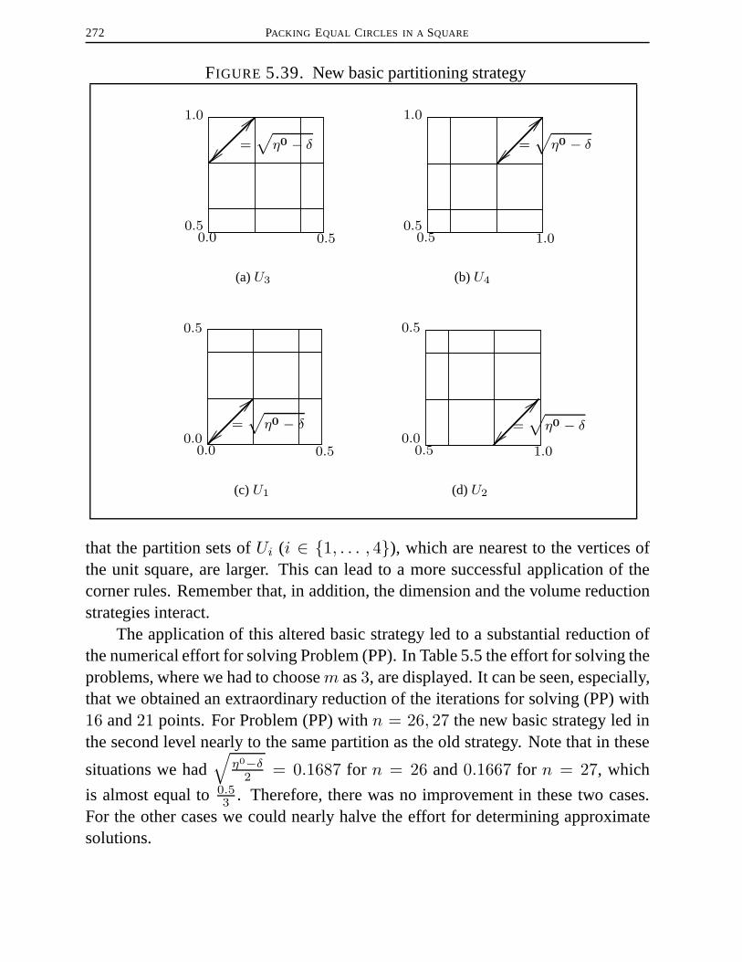
272 PACKING EQUAL CIRCLES IN A SQUARE
FIGURE 5.39. New basic partitioning strategy
0.0
1.0
0.50.5
=√
η0 − δ
(a)U3
0.5
1.0
0.51.0
=√
η0 − δ
(b) U4
0.0
0.5
=√
η0 − δ0.0
0.5
(c) U1
0.5
0.5
0.01.0
=√
η0 − δ
(d) U2
that the partition sets ofUi (i ∈ {1, . . . , 4}), which are nearest to the vertices ofthe unit square, are larger. This can lead to a more successful application of thecorner rules. Remember that, in addition, the dimension and the volume reductionstrategies interact.
The application of this altered basic strategy led to a substantial reduction ofthe numerical effort for solving Problem (PP). In Table 5.5 the effort for solving theproblems, where we had to choosem as3, are displayed. It can be seen, especially,that we obtained an extraordinary reduction of the iterations for solving (PP) with16 and21 points. For Problem (PP) withn = 26, 27 the new basic strategy led inthe second level nearly to the same partition as the old strategy. Note that in these
situations we had√
η0−δ2 = 0.1687 for n = 26 and0.1667 for n = 27, which
is almost equal to0.53 . Therefore, there was no improvement in these two cases.For the other cases we could nearly halve the effort for determining approximatesolutions.

5.8. IMPROVEMENTS OFALGORITHM 5.1 273
TABLE 5.5. Numerical effort with altered basic strategyn IT TT NLP TLP NR MNPS14 6,651 24.1 340 3.97 18,015 70215 1,532 6.30 158 2.22 3,590 25516 1,832 7.24 150 2.11 4,401 17617 17,023 113 2,371 44.0 38,718 1,37318 10,446 101 2,306 54.3 21,861 49419 29,046 130 1,239 30.0 60,514 1,92720 13,374 180 4,440 107 26,161 48821 82,865 771 11,885 314 161,072 5,59022 33,644 281 3,331 102 62,579 2,66923 86,412 1,549 26,750 953 154,418 4,77824 103,557 1,431 17,285 697 177,526 7,00725 66,900 1,066 12,324 554 111,056 4,37626 661,811 9,024 46,472 2,291 1,034,886 36,33527 251,004 3,204 13,656 799 365,210 15,457
In the implementation of Algorithm 5.1, whose results are reported in Table5.5, we also altered the selection rule of the current hyperrectangleRk+1 in StepVII of our method. Instead of choosingRk+1 among all hyperrectanglesR ∈ Rk+1
with a lower bound equal toµk+1, we select, if possible, a child ofRk with thisattribute. Note that in the old strategy we applied the FIFO principle, i.e., first-in-first-out, and that the new strategy is related to the LIFO principle, i.e., last-in-first-out. Our numerical experience showed that this selection strategy nearly halved themaximal number of stored partition sets (see the casesn = 26, 27 in Table 5.5 andremember that in these cases the new basic strategy had almost no influence).
5.8.2. Altered Decision Criterion. In the previous section we described acriterion according to which we decide, whether we calculate an upper bound forthe current hyperrectangleRkp (p ∈ {1, . . . , l}) by solving a linear program orwhether we choose the old upper boundµk, respectively the updated oneµRkp =min{µk, µRkp} (see (5.7.1)). This criterion based on the check of the feasibility ofa pointx ∈ Un with respect to the linear subproblem (LSP’) (see page 264), wherethe members of this point are vertices of the rectangles formingRkp . Taking thelarge number of possible points into account the verification of this criterion can betime-consuming. Nevertheless, the application of this strategy lead to an essentialreduction of the running-times. The following cheap and simple decision criterionshowed even better results.
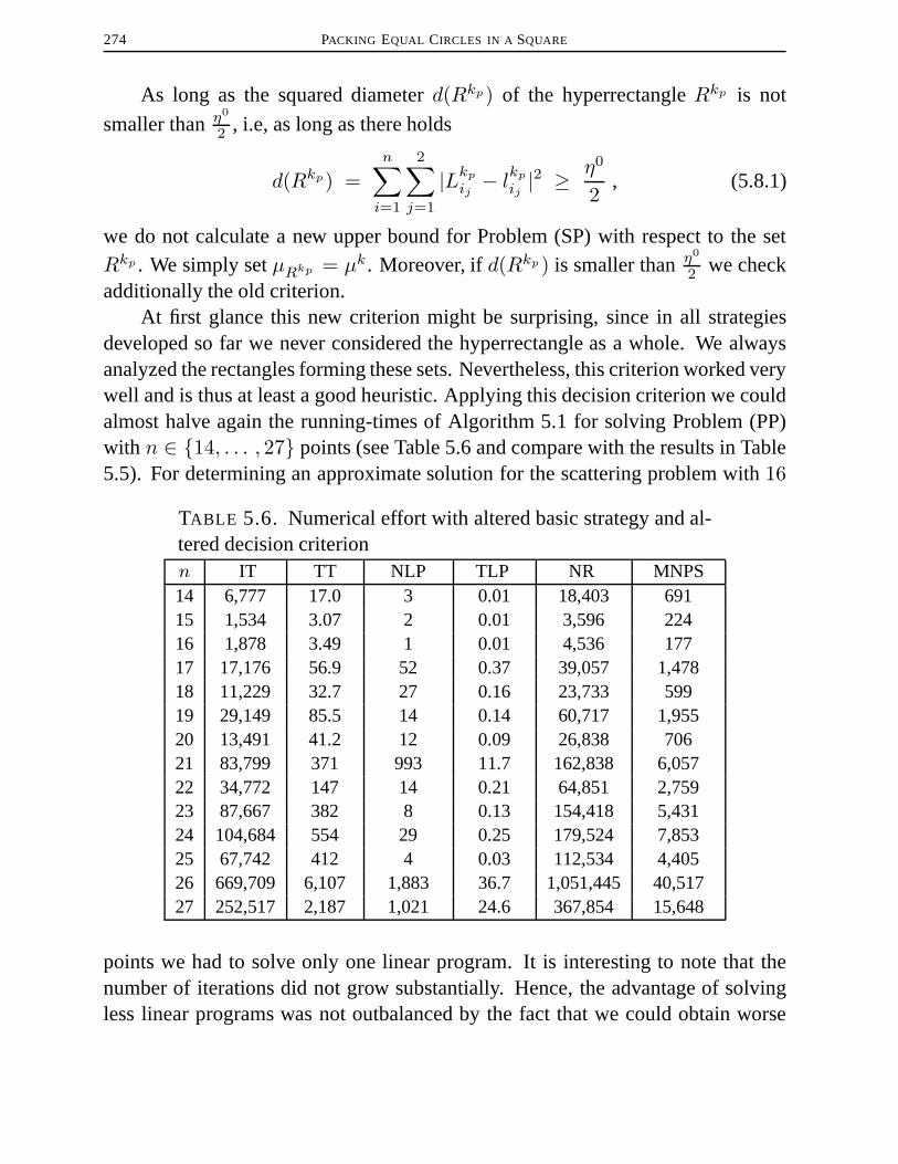
274 PACKING EQUAL CIRCLES IN A SQUARE
As long as the squared diameterd(Rkp) of the hyperrectangleRkp is not
smaller thanη0
2 , i.e, as long as there holds
d(Rkp) =n∑i=1
2∑j=1
|Lkp
ij− lkp
ij|2 ≥ η0
2, (5.8.1)
we do not calculate a new upper bound for Problem (SP) with respect to the setRkp . We simply setµRkp = µk. Moreover, ifd(Rkp) is smaller thanη
0
2 we checkadditionally the old criterion.
At first glance this new criterion might be surprising, since in all strategiesdeveloped so far we never considered the hyperrectangle as a whole. We alwaysanalyzed the rectangles forming these sets. Nevertheless, this criterion worked verywell and is thus at least a good heuristic. Applying this decision criterion we couldalmost halve again the running-times of Algorithm 5.1 for solving Problem (PP)with n ∈ {14, . . . , 27} points (see Table 5.6 and compare with the results in Table5.5). For determining an approximate solution for the scattering problem with16
TABLE 5.6. Numerical effort with altered basic strategy and al-tered decision criterionn IT TT NLP TLP NR MNPS14 6,777 17.0 3 0.01 18,403 69115 1,534 3.07 2 0.01 3,596 22416 1,878 3.49 1 0.01 4,536 17717 17,176 56.9 52 0.37 39,057 1,47818 11,229 32.7 27 0.16 23,733 59919 29,149 85.5 14 0.14 60,717 1,95520 13,491 41.2 12 0.09 26,838 70621 83,799 371 993 11.7 162,838 6,05722 34,772 147 14 0.21 64,851 2,75923 87,667 382 8 0.13 154,418 5,43124 104,684 554 29 0.25 179,524 7,85325 67,742 412 4 0.03 112,534 4,40526 669,709 6,107 1,883 36.7 1,051,445 40,51727 252,517 2,187 1,021 24.6 367,854 15,648
points we had to solve only one linear program. It is interesting to note that thenumber of iterations did not grow substantially. Hence, the advantage of solvingless linear programs was not outbalanced by the fact that we could obtain worse

5.8. IMPROVEMENTS OFALGORITHM 5.1 275
upper bounds. Note that, if we do not solve (LSP’), we save time since we donot callMINOS 5.4 and, additionally, we save time since we do not construct theLP-relaxation of Problem (SP).
A reason for the good performance of Algorithm 5.1 using this criterion mightbe the following. Our numerical experience showed that the subdivision set mani-pulation strategies are really successful in detecting areas ofUn, where no optimalsolution exists. Moreover, they are able to significantly reduce the size of the re-maining sets containing solutions of Problem (PP). However, if these sets getsmalland the best known solution is maybe not good enough, the manipulation strategiesdo not result in further progress. In this situation it is useful to calculate upperbounds by solving the LP-relaxation of (SP). Doing this we can obtain slight im-provements of the best known solution and we diminish the distance between thelower and the upper bounds. The described criterion seems to be a good choice fordetecting such situations, where the considered hyperrectangles aresmall.
We tested also several other criteria, which were not as keen as the above one.For instance, we required that each rectangleR
kp
i (i ∈ {1, . . . , n}) was subdividedtwice, i.e., that there held
maxi=1,... ,n
maxj=1,2
|Lkp
ij− lkp
ij| <
√η0
2.
Using these criteria the running-times always increased on average.On the other hand we tested additionally a variant of Algorithm 5.1, where we
never calculate an upper bound by solving a linear program. We always chose thesimple upper boundµRkp = min{µk, µRkp } with µRkp given as in (5.7.1). Doingthis the running-times explode for the most examples. Hence, even though we havein comparison with the number of considered hyperrectangles only a small numberof linear problems to solve, the solution of these problems is necessary in order toobtain an efficient method for solving the point scattering problem.
5.8.3. Solutions of Problem (PP) with more than 27 Points.In the previoussection we pointed out that we were not able to solve Problem (PP) with more than27 points, at least with the version of Algorithm 5.1 used there. The improvementsof Algorithm 5.1 developed in the present section enabled us to solve such prob-lems. However, in comparison to the casesn ≤ 27 the running-times still explode.
In order to obtain approximate solutions for Problem (PP) withn > 27 weused a"parallelized"variant of Algorithm 5.1. At first we generated all possiblehyperrectanglesR = R1 × . . .×Rn with the property that each rectangleRj was
276 PACKING EQUAL CIRCLES IN A SQUARE
subdivided once, i.e., coincides with one of the squaresUj (j ∈ {1, . . . , 4}, see(5.5.1)). After this we used each of these hyperrectangles as the initialization setfor Algorithm 5.1. In this way we could use several machines in order to solveProblem (PP). Apart form theSUN ULTRA 60 workstations used till now, weadditionally appliedSUN Server 1000workstations. These machines are – withour code – on average 4 times slower.
In order to avoid excessive storage requirements we used the depth-first-search-strategy mentioned in Remark 5.7.2(b). Since we did not know the coordinates ofthe best known solutions for Problem (PP) withn > 27 we did not initializex0.We initialized onlyη0.
REMARK 5.8.1. The coordinates ofx, which is used for the initialization ofx0, are not substantial for Algorithm 5.1. This methods needs only a good ap-proximation forη0. Therefore, it is sufficient if we setη0 without knowing thecoordinates ofx. Moreover, if we initializeη0 with η − ε, whereη is the best pub-lished value, we can guarantee that Algorithm 5.1 delivers the coordinates of anε-optimal solution.
Since we used the best known solutions given in [NO97] we had to choosem = 4 in the second level of our basic partitioning strategy in order to solve Prob-lem (PP) with more than27 points. According to our new partitioning strategy therectanglesUi (i ∈ {1, . . . , 4}) were hence partitioned into9 squares with edge-
length√
η0−δ2 and7 additional rectangles. Thus the number of possibilities for
settingRki
j (j ∈ {1, . . . , n}, i ∈ {1, . . . , l}, k ∈ IN) in Step III of Algorithm 5.1was substantially larger than by choosingm = 3, as it was the case forn ≤ 27.With respect to our subdivision set manipulation strategies and the fact that therewere7 small rectangles we still hoped to be able to solve (PP) with acceptablecomputational effort. However, even the fastest one (see casen = 30 in Table 5.7)could not be solved within one day, and hence we could not expect to solve manycases withn > 27.
The numerical effort for solving Problem (PP) withn ∈ {28, 29, 30, 31} isshown in Table 5.7. We used again the accuracyε = 10−5, except forn = 31we appliedε = 5 ∗ 10−5. The abbreviations are the same as before. However, therunning-times are given in hours. The additional column NP shows the number ofpossible hyperrectangles after the first level, i.e., the number of different problemswe solved in order to obtain an approximate solution of the corresponding pointscattering problem. Since we solved each problem using different machines we

5.8. IMPROVEMENTS OFALGORITHM 5.1 277
TABLE 5.7. Numerical effort for solving (PP) withn > 27n NP IT TT NLP TLP NR η?
28 29 86,848,406 205.44 7,149 0.04 206,979,450 0.053142729 21 38,423,801 103.23 109 0.01 96,339,168 0.051473930 16 11,034,381 27.71 8 0.00 24,955,286 0.050398731 9 76,263,071 229.39 4,802,901 42,57 164,774,004 0.047324
added the effort needed for each process. In order to obtain comparable running-times we scaled the times obtained with theSUN Server 1000workstations with thespeedup-factor4.0 mentioned before. Thus the running-times displayed in Table5.7 are approximations of the necessary time for completely solving these problemson aSUN ULTRA 60 workstation.
It is interesting to note that even though there are nearly double as much pos-sibilities in the second partitioning level as for the casesn ≤ 27, the number ofconsidered hyperrectangles in Step IV is still less than three times the number ofiterations. This corroborates again the success of the special features of the subdi-vision strategy. As in the cases considered in the previous section we did not de-termine solutions of Problem (PP) (see columnη?) with a larger minimum squaredpairwise distance than the best known so far.
Our numerical experience for the casen = 31 showed that in this case a sym-metry avoiding strategy in the third level could improve the numerical performanceof Algorithm 5.1. Note that for the casesn ≤ 27 we pointed out that it was notuseful to use this strategy in deeper levels than the second one. In Figures 5.40-5.42we show again the arrangements of the calculatedε-optimal solutions together with
FIGURE 5.40. Solution forn = 28
0
1
1
x1 = (0.0000, 1.0000) x2 = (1.0000, 1.0000)
x3 = (0.0000, 0.0060) x4 = (1.0000, 0.2170)
x5 = (0.0000, 0.6333) x6 = (1.0000, 0.6163)
x7 = (0.0000, 0.2365) x8 = (0.2305, 0.0000)
x9 = (0.9221, 0.0000) x10 = (0.2833, 1.0000)
x11 = (0.7444, 1.0000) x12 = (0.2305, 0.2305)
x13 = (0.4601, 0.0000) x14 = (0.4996, 0.2273)
x15 = (0.1175, 0.4349) x16 = (0.3672, 0.4161)
x17 = (0.6915, 0.0000) x18 = (0.7695, 0.2170)
x19 = (0.6417, 0.4088) x20 = (0.8847, 0.4166)
x21 = (0.2569, 0.6185) x22 = (0.1417, 0.8181)
x23 = (0.3986, 0.8003) x24 = (0.5119, 0.5994)
x25 = (0.7569, 0.6085) x26 = (0.6291, 0.8003)
x27 = (0.5139, 1.0000) x28 = (0.8722, 0.8081)

278 PACKING EQUAL CIRCLES IN A SQUARE
their coordinates.
FIGURE 5.41. Solutions forn = 29, 30
1
10
(a)n = 29
x1 = (0.0000, 1.0000) x2 = (0.0000, 0.0450)
x3 = (1.0000, 0.2051) x4 = (1.0000, 0.5981)
x5 = (1.0000, 1.0000) x6 = (0.0000, 0.7237)
x7 = (0.0000, 0.4969) x8 = (0.2224, 0.0000)
x9 = (0.9030, 0.0000) x10 = (0.3193, 1.0000)
x11 = (0.0204, 0.2709) x12 = (0.3194, 0.2051)
x13 = (0.4493, 0.0000) x14 = (0.2059, 0.4016)
x15 = (0.4328, 0.4016) x16 = (0.6761, 0.0000)
x17 = (0.5462, 0.2051) x18 = (0.7731, 0.2051)
x19 = (0.6597, 0.4016) x20 = (0.8860, 0.4016)
x21 = (0.3194, 0.5981) x22 = (0.2140, 0.7990)
x23 = (0.4409, 0.7990) x24 = (0.5462, 0.5981)
x25 = (0.7731, 0.5981) x26 = (0.6678, 0.7790)
x27 = (0.5462, 1.0000) x28 = (0.8947, 0.7790)
x29 = (0.7731, 1.0000)
0
1
1
(b) n = 30
x1 = (1.0000, 0.2000) x2 = (0.0000, 0.8000)
x3 = (0.0000, 0.4000) x4 = (0.0000, 0.0000)
x5 = (1.0000, 0.6000) x6 = (1.0000, 1.0000)
x7 = (0.8980, 0.0000) x8 = (0.1020, 1.0000)
x9 = (0.2245, 0.0000) x10 = (0.1020, 0.2000)
x11 = (0.4490, 0.0000) x12 = (0.3265, 0.2000)
x13 = (0.2245, 0.4000) x14 = (0.4490, 0.4000)
x15 = (0.6735, 0.0000) x16 = (0.5510, 0.2000)
x17 = (0.7755, 0.2000) x18 = (0.6735, 0.4000)
x19 = (0.8980, 0.4000) x20 = (0.1020, 0.6000)
x21 = (0.3265, 0.6000) x22 = (0.2245, 0.8000)
x23 = (0.4490, 0.8000) x24 = (0.3265, 1.0000)
x25 = (0.5510, 0.6000) x26 = (0.7755, 0.6000)
x27 = (0.6735, 0.8000) x28 = (0.5510, 1.0000)
x29 = (0.8980, 0.8000) x30 = (0.7755, 1.0000)
We also tried to solve even larger problems. However, the point scatteringproblem with32 points could not be solved within two weeks. Hence we do notexpect that the current version of Algorithm 5.1 is able to solve Problem (PP) withn > 31 within several days, and we did not try this until now. Nevertheless, in thissection we saw that slight changes of some strategies can essentially improve thenumerical performance of Algorithm 5.1. Consequently, we hope that it is possibleto modify the presented strategies as well as to develop new strategies in order to

5.8. IMPROVEMENTS OFALGORITHM 5.1 279
FIGURE 5.42. Solution forn = 31
1
0 1
x1 = (1.0000, 0.7828) x2 = (1.0000, 0.1061)
x3 = (0.0000, 0.8101) x4 = (0.0000, 0.4351)
x5 = (1.0000, 0.5497) x6 = (1.0000, 0.3292)
x7 = (0.9870, 1.0000) x8 = (0.8101, 0.0000)
x9 = (0.1061, 1.0000) x10 = (0.4351, 0.0000)
x11 = (0.5496, 1.0000) x12 = (0.3290, 1.0000)
x13 = (0.0000, 0.0000) x14 = (0.2175, 0.0000)
x15 = (0.0000, 0.2175) x16 = (0.2175, 0.2175)
x17 = (0.4351, 0.2206) x18 = (0.2206, 0.4351)
x19 = (0.4382, 0.4382) x20 = (0.6226, 0.1103)
x21 = (0.8132, 0.2176) x22 = (0.6257, 0.3279)
x23 = (0.8125, 0.4394) x24 = (0.1103, 0.6226)
x25 = (0.3279, 0.6257) x26 = (0.2175, 0.8132)
x27 = (0.4393, 0.8125) x28 = (0.6115, 0.5696)
x29 = (0.8107, 0.6570) x30 = (0.6568, 0.8107)
x31 = (0.7685, 0.9979)
further improve the suggested method. This might lead to an approach, which iseven able to solve larger problems with acceptable effort. Recognize that Problem(PP) withn > 30 is – from a deterministic global optimization point of view –a huge problem. The small numbers of linear programs, which had to be solvedduring the execution of Algorithm 5.1 (see the corresponding columns in Table 5.6and Table 5.7), let expect that a further modification of the upper bounds will notlead to a faster approach. The key for the acceleration of Algorithm 5.1 are thesubdivision set manipulation strategies.
Let us finish this chapter with a good solution of Problem (PP) with32 points
FIGURE 5.43. Good solution forn = 32
0
1
1
x1 = (1.0000, 1.0000) x2 = (1.0000, 0.0594)
x3 = (0.0000, 0.7953) x4 = (1.0000, 0.6987)
x5 = (0.0000, 0.4262) x6 = (0.7953, 0.0000)
x7 = (0.0594, 1.0000) x8 = (0.6987, 1.0000)
x9 = (0.4262, 0.0000) x10 = (0.0000, 0.0000)
x11 = (0.2131, 0.0000) x12 = (0.0000, 0.2131)
x13 = (0.2131, 0.2131) x14 = (0.4262, 0.2131)
x15 = (0.2131, 0.4262) x16 = (0.4262, 0.4262)
x17 = (0.6108, 0.1066) x18 = (0.7953, 0.2131)
x19 = (1.0000, 0.2725) x20 = (0.6108, 0.3197)
x21 = (0.7953, 0.4262) x22 = (1.0000, 0.4856)
x23 = (0.1066, 0.6108) x24 = (0.3197, 0.6108)
x25 = (0.2131, 0.7953) x26 = (0.2725, 1.0000)
x27 = (0.4262, 0.7953) x28 = (0.4856, 1.0000)
x29 = (0.5872, 0.5872) x30 = (0.7938, 0.6393)
x31 = (0.6393, 0.7938) x32 = (0.8459, 0.8459)

280 PACKING EQUAL CIRCLES IN A SQUARE
detected during our numerical tests. The solution displayed in Figure 5.43 has aminimum squared pairwise distance ofmin1≤i<j≤32 ‖xi − xj‖22 = 0.0454068,which is slightly better than the one given in [NO97] (0.04540409). This is theonly case, where we detected by applying Algorithm 5.1 a better solution than thebest known so far.

CHAPTER 6
Conclusion
We would like to complete this doctoral thesis with a short review of the topics wetreated. What have we reached and which questions are still to be answered?
The main aim of this dissertation was the development and the theoretical aswell as numerical examination of solution methods for so-callednonconvex all-quadratic optimization problems, i.e., for problems of type
min xTQ0x+ (d0)Tx
xTQlx+ (dl)Tx+ cl ≤ 0 l = 1, . . . , p
x ∈ P ,
(QP)
with Ql ∈ IRn×n symmetric,dl ∈ IRn (l = 0, . . . , p), cl ∈ IR (l = 1, . . . , p)andP = {x ∈ IRn : Ax ≤ b} a non-empty, full-dimensional polytope withA ∈ IRm×n andb ∈ IRm. We proposed two, respectively three new approaches forsolving this class of global optimization problems.
The first method was developed for the solution of so-calledunary problems.This class of optimization problem was of interest, since each problem of type(QP) can be transformed into a unary program. With some technical effort we de-rived several convergent solution approaches for this type of global optimizationproblems. Hence we overcome the theoretical deficiency of an outer approxima-tion scheme given by Ramana [RAM 93], which was the only solution approach forunary problems known so far. Our algorithms are combinations of outer approx-imations and – branch-and-bound like – successive subdivisions of the feasibleregion. One variant of these new methods uses a regularn-simplex with all itsvertices on the boundary of the Euclidean unit ball. Even though the properties ofsuch ann-simplex are known in the literature, to the author’s knowledge there isno explicit construction of such a set – except in the present work and in [HR98].
281

282 CONCLUSION
Unfortunately, the indirect approach for solving (QP) via the solution of thecorresponding unary program is only of theoretical interest. The numerical resultsshowed that this method is not able to solve all-quadratic problems with accept-able computational effort. Excessive numerical effort was needed in order to solvethe unary problems resulting from the transformation of the all-quadratic problemsbelonging to our randomly generated test set.
The numerical effort for solving a unary problem depends substantially onthe structure of the affine matrix mapping forming the single nonlinear constraint.For unary problems resulting from the transformation of all-quadratic problemsthis mapping has an unpleasant structure. If unary problems with an easier matrixmapping are considered it is likely that our methods show a substantially betternumerical performance. Moreover, in such a case it could even be interesting tochange some features of Algorithm 2.3 in order to further improve its numericalperformance (see the considerations at the end of Chapter 2). However, anotherapplication of unary problems, which could lead to a simpler matrix mapping, isnot known to our knowledge.
As mentioned before, we developed a new method for the solution of unaryproblems since the convergence of the outer approximation scheme proposed byRamana is not provable. This is a theoretical problem of several algorithms, whichbase on cutting planes, developed for global optimization problems (see, e.g.,[HT96B]). It might be that the ideas used in Chapter 2 in order to obtain a con-vergent algorithm can also be applied for other problem classes, where the conver-gence of corresponding outer approximation schemes is not known. Hence, thereare some theoretically interesting aspects of the content of Chapter 2, even thoughwe did not reach our main goal to obtain practicable solution methods for problemsof type (QP).
The second solution approach for Problem (QP) suggested in Chapter 3 wasmore successful with respect to this main intention of the present thesis. Thepresented simplicial branch-and-bound method showed a good numerical perfor-mance, at least for the solution of arbitrary problems of type (QP) with a dimensionless than10. Beside the rectangular branch-and-bound algorithm introduced in[AKLV95] our simplicial method belongs to the rare approaches in the literature,which consider Problem (QP) directly. Other solution approaches for all-quadraticproblems mostly interpret this type of programs as a special instance of a more gen-eral problem class, like bilinear problems [AK92], polynomial problems [ST92],

CONCLUSION 283
problems involving biconvex functions [FV93B], general d.c. problems (see Chap-ter 4) or – as we did in Chapter 2 – unary problems [RAM 93].
As long as an exhaustive subdivision rule for then-simplices considered in ouralgorithm is used the convergence of our method can be ensured. Hence, this sim-plicial algorithm has the same theoretical properties as the comparable rectangularapproach by Al-Khayyal et al. [AKLV95]. Moreover, numerically, our methodoften outperforms this rectangular approach, in particular when all-quadratic prob-lems with more quadratic constraints than the dimensions, i.e.,p > n, have to besolved. The complexity of the LP-relaxations used in our approach, i.e., their di-mension and number of linear constraints, depends linearly onp andn. In contrastto this the LP-relaxations applied in Al-Khayyal et al.’s method for the calculationof lower bounds have a dimension of(p+ 2)n and4(p+ 1)n+ p+m linear con-straints. The less complex relaxations in our approach are the main reason for thebetter numerical performance.
If we are interested in a practicable approach for solving (QP), convergence ofsuch an algorithm is not sufficient. In addition we need that the method is finite.However, this can only be obtained, if we are satisfied with approximate solutions.In particular, we have to be satisfied with solutions of Problem (QP), which are ap-proximately feasible, i.e., fulfill the constraints up to a prespecified tolerance, andwhich are, additionally, approximately optimal. The solution methods consideredin this thesis can determine such approximate solutions in finite time. In contrastto other global optimization problems, like concave minimization, it is in generalnot possible to require that the determined approximate solution of Problem (QP)is at least feasible. Note that the problem of detecting a feasible point for this typeof problems is as hard as the solution of (QP) itself. However, under additional as-sumptions the feasibility of calculated solutions could be guaranteed. For instance,if we require that the feasible region of (QP) contains a ball with known radius, thenit is possible to choose the accuracies in our simplicial method such that Algorithm3.1 determines a feasible point in finite time. Our first method and the general-ization of the simplicial branch-and-bound approach considered in Chapter 4 canalso be adapted in this way. However, the verification of such a strict assumption isagain a hard problem, unless the examined instance of Problem (QP) has a specialstructure.
In the definition of our simplicial branch-and-bound method there are stillsome features, which could be modified or changed in order to affect the numeri-cal behavior of this approach. At the end of Chapter 3 we saw, for example, that

284 CONCLUSION
the exploitation of the fact that the LP-relaxations applied in our approach are notuniquely determined can improve the performance of Algorithm 3.1. Another fea-ture of this method, which could be changed, is the subdivision rule. We usebisec-tion, where a partition of the currentn-simplex is performed by a radial subdivisionwith respect to the midpoint of the longest edge. This subdivision rule is exhaus-tive. The same holds for thegeneralized bisectionmentioned on page 127. Hence,this rule could also be applied without altering the theoretical properties of ourapproach.
In the context of simplicial branch-and-bound methods for the minimizationof concave functions with respect to polytopes, i.e., forconcave minimizationproblems, the so-calledω-subdivision is favored by some authors. In this rulethe currentn-simplexS is partitioned into up ton + 1 subsimplices by applyinga radial subdivision with respect to the point, where the optimal solution of theLP-relaxation on the setS is attained. Using this rule one hopes to obtain bet-ter numerical results, since the subdivision point is more related to the problemthan the midpoint of the longest edge used in the bisection rule. However, it wasan open question, whether simplicial branch-and-bound methods employing onlyω-subdivisions are convergent, since this subdivision rule is not necessarily exhaus-tive.
We were first of all interested in convergent solution approaches for Problem(QP). Therefore, we had to answer this open question, if we wanted to apply theω-subdivision rule in our simplicial branch-and-bound method. The ideas used inChapter 3 in order to develop a solution approach for (QP) could analogously beused for deriving a simplicial branch-and-bound algorithm for the solution of so-calledgeneralized d.c. problemscontaining the class of all-quadratic problems aswell as the class of concave minimization problems. Therefore, we tried to answerthe open question mentioned above for the generalized algorithm introduced inChapter 4, which is able to solve such d.c. programs.
We proved that for general d.c. problems and in particular for general all-quadratic problems our algorithm can fail to converge, if onlyω-subdivisions areemployed. However, if this method is applied for concave minimization problemsor for problems with a d.c. objective function – consisting of a quadratic convexpart and a strictly concave part – and with concave and linear constraints, the con-vergence even withω-subdivisions can be guaranteed. This was the main resultin Chapter 4. Note that the convergence of this method could only be guaranteed

CONCLUSION 285
in the sense that this approach detects for arbitrary accuraciesε, δ > 0 either theemptiness of the feasible region or an (ε, δ, 0)-solution of the considered problemin finite time. This convergence result was theoretically weaker than the other con-vergence results examined in this thesis. Nevertheless, – from a practical point ofview – all results have the same quality. They ensure the finiteness of our methods,if we are satisfied with approximate solutions.
Apart from these convergence results we were, furthermore, able to prove thatthis method withω-subdivisions delivers in finite time even the optimal solutionof a concave minimization problem, if two additional assumptions are fulfilled. Itdoes not seem that this finiteness result can be extended to more general problemclasses, since for the proofs it was essential that the feasible set is a polytope. Onthe other hand, it is an interesting question whether the additional assumptionscould be weakened without losing the finiteness result.
We also examined the numerical performance of the introduced generalizedsimplicial branch-and-bound Algorithm 4.1 with respect to problems of type (QP).Since this algorithm uses convex relaxations instead of LP-relaxations applied byAlgorithm 3.1, we were at first interested in a numerical comparison of both ap-proaches only using bisections. Note that the generalized algorithm is always con-vergent, if an exhaustive subdivision rule is used – as it is the case for Algorithm3.1. We observed that the version of Algorithm 4.1, which employs only bisec-tions, can be expected to be numerically more efficient than Algorithm 3.1, at leastas long as a solver for the convex relaxations is used, which exploits the quadraticstructure of the involved functions.
The main aim for consideringω-subdivisions in Chapter 4 was the hope to ob-tain an algorithm showing a better numerical performance than a method, whichsimply chooses bisection. As mentioned before, we know that in general the con-vergence of an approach, which employs onlyω-subdivisions, cannot be ensured.However, our theoretical results derived in Chapter 4 enabled us to develop a mixedsubdivision strategy (MGWSR) – consisting of bisections andω-subdivisions –leading to a convergent approach for solving general d.c. problems. Note that(MGWSR) is different form the mixed strategy used in the so-callednormal sim-plicial branch-and-bound algorithms. Unfortunately, the numerical tests using thismixed strategy (MGWSR) and variants of it were really disappointing. Even thoughAlgorithm 4.1 using (MGWSR) had a good performance for a few test examples,on average the application of this rule results in a substantially worse numeri-cal performance than the use of bisection. We did not find a strategy based on
286 CONCLUSION
(MGWSR), which has the best numerical performance in all test examples, i.e.,which is the fastest one, if (MGWSR) leads faster to a solution than bisection aswell as if bisection is faster than (MGWSR). It is hence still an open questionwhether there exists a subdivision rule for simplicial branch-and-bound methods,which always shows the best numerical behavior. We believe that such a rule doesnot exist in general. Taking the structure of special problem instances into accountit might be non the less possible to develop a subdivision rule, which has this prop-erty, at least as long as the resulting algorithm is applied for the solution of theseinstances.
Till Chapter 4 we developed two new approaches for the solution of the gen-eral form of Problem (QP). Note that Algorithm 3.1 can be interpreted as a specialcase of Algorithm 4.1. In the introduction of this thesis (see Section 1.1) we sawthat there are many applications of this type of global optimization problems. Con-sequently, it was interesting to examine such a special instance of Problem (QP).We chose the problem of packingn ∈ IN equal and non-overlapping circles withmaximum radius into the two-dimensional unit square, which we called thepackingproblem. The optimal solutions of this problem with up to20 circles are reported tobe known. Hence, we had to solve an all-quadratic problem (see page 189) with adimension higher than40, if we wanted to determine new global optimal solutions.From a global optimization point of view, such problems are very large. Thus, itwas not really surprising that our general methods for (QP) developed so far fail tosolve the packing problem with more than20 circles and acceptable effort.
In the considerations of our general schemes we often claimed that the ex-ploitation of the structure of special problem instances can improve their numer-ical performance. This was particularly the case with the packing problem. Wesuggested a rectangular branch-and-bound algorithm, which was able to solve thepacking problem with up to27 circles within two hours.
We exploited the special structure of the packing problem, respectively of theall-quadratic formulation (PP) of the equivalentpoint scattering problemin differ-ent ways. First of all we derived some new theoretical results showing the existenceof a solution of this problem with a special behavior on the boundary of the unitsquare. In particular, we proved that there is an optimal solutionx? consisting ofn two-dimensional membersx?i (i = 1, . . . , n) such that for each vertexv of theunit square there holds: Either the vertexv is itself a member ofx? or there aretwo members of this solution belonging to the boundary lines of the unit square

CONCLUSION 287
forming this vertex, which have exactly the optimal distance from each other. Eventhough we do not know an optimal solution of the point scattering problem with theproperty that no vertex of the unit square is a member of this solution, we were notable to prove this fact. We could not show that at least one vertex has to belong toan optimal solution of the point scattering problem. This is still an open question.The existence of optimal solutions with the proven behavior on the boundary of theunit square could be used in order to reduce the number of possible solutions of theconsidered problem, which our algorithm has to look for.
Apart from the derivation of these theoretical results we exploited the structureof the packing problem in the construction of LP-relaxations, which are neededfor the calculation of bounds. These special relaxations are better than those ob-tained by general approaches. We could also use the structure of the consideredinstance of (QP) in order to develop special subdivision strategies for the relevanthyperrectangles. Moreover, we were able to derive further powerful subdivision setmanipulation strategies. Note that the derivation of such strategies is mostly notpossible, if general problem classes are considered.
The combination of all these adjustments of a general rectangular branch-and-bound scheme to a special problem instance led to a really successful solutionapproach for the packing problem. The proposed algorithm is able to prove theε-optimality of determined approximate solutions. Hence, this approach could beused as a computer aided proof, since the optimal solutions of the packing problemfor more than20 circles are mostly not known and since our numerical experienceshowed that Algorithm 5.1 is able to solve problems with these sizes and acceptableeffort. We pointed out that our current implementation of Algorithm 5.1 cannot beused without reservation as a computer aided proof. Nevertheless, it is possible toadapt this implementation such that the required precision can be reached.
The performance of the proposed method depends essentially on the qualityof the solutions of the examined problem known in advance. Algorithm 5.1 isnot applicable in order to determine new solutions of the packing problem with-out knowing good initial approximations. The main advantage of our method isthe possible guarantee of theε-optimality of determined points mentioned before.Nevertheless, this approach can also detect better solutions than the best known sofar, as we saw for the case with32 circles.

288 CONCLUSION
The suggested strategies for improving the performance of Algorithm 5.1 aresurely not yet the best ones. We believe that there are still further possible im-provements, especially for the subdivision set manipulation strategies, such thateven larger examples of the packing problem can be solved globally.
The last chapter of this thesis showed that an adjustment of a general solutionscheme to a special problem instance can significantly improve the numerical per-formance of the method applied for the solution of this instance. Moreover, we sawthat in global optimization general approaches are – from a practical point of view– often not able to solve problems resulting from applications, since the sizes ofthese problems are too large. Another interesting aspect of Chapter 5 is that the keyfor the acceleration of the branch-and-bound Algorithm 5.1 was not the develop-ment of good relaxations for calculating bounds. The subdivision set manipulationstrategies were decisive. Also for other problem instances it is possible that theexamination of the structure of the feasible region and the resulting derivation ofsubdivision set manipulation strategies is – with respect to the numerical perfor-mance of a branch-and-bound method – more successful than the development ofspecial bounds.

APPENDIX A
Proofs for Section 4.4
Before expatiating the longer and more technical proofs of some results proposedin Section 4.4 we first establish a lemma, which will ease our work. The statementof this lemma does not depend on the problem class which we would like to solvewith Algorithm 4.1.
LEMMA A.1. Let{Sk}k∈IN be an infinite nested simplex sequence generatedby Algorithm 4.1 with Properties (4.4.2.a) and (4.4.2.b), and let{xk}k∈IN be apoint sequence withxk ∈ Sk (k ∈ IN). Chooseλk ∈ Bn such that, for allk ∈ IN,
xk =n∑i=0
λki vki . (A.0.1)
Assume that there is an indexi′ ∈ {0, . . . , n} such that the verticesvki′ (k ∈ IN)change infinitely often, i.e.,
|{k ∈ IN : vk+1i′ 6= vki′}| = ∞ , (A.0.2)
and such that there holds
λki′ 6→ 0 (k →∞) . (A.0.3)
Then there exist an indexl ∈ {0, . . . , p}, a positive real numberτ and a subse-quence{kq}q∈IN of {k}k∈IN satisfying, for allq ∈ IN,
ϕlSkq (xkq ) ≥ ϕl
Skq−1 (xkq ) + τ . (A.0.4)
In particular, there holds
ϕ0Skq (xkq ) ≥ ϕ0
Skq−1 (xkq ) + τ ,
if all elements of the vertex sequence{vki′}k∈IN are (δ, 0)-feasible.
289

290 PROOFS FORSECTION 4.4
PROOF FOR (DCP1) AND (DCP2): The boundedness of the sequence{λki′}k∈IN implies that there is a convergent subsequence{λkq
i′ }q∈IN satisfying
λkq
i′ → 2ν (q →∞)
for a positive real valueν. It follows that there exists a numberQ ∈ IN with theproperty that, for allq ≥ Q, there holds
λkq
i′ > ν .
We assume, without loss of generality, thatQ = 1. Regarding (A.0.2) we areable to choose the subsequence{λkq
i′ }q∈IN in a way such that each member of the
corresponding vertex sequence{vkq
i′ }q∈IN is different from his successor, i.e.,
∀q ∈ IN vkq+1i′ 6= v
kq
i′ .
Therefore, we know that, for allq ∈ IN, there exists an indexkq(i′) < kq,kq(i′) ≥ kq−1 – not necessarily belonging to the subsequence{kq}q∈IN – with
vkq
i′ = ω(Skq(i′)) .
Thus, for eachq ∈ IN, there holds
Skq(i′)+1 = [vkq(i′)0 , . . . , v
kq(i′)i′−1 , v
kq
i′ , vkq(i′)i′+1 , . . . , v
kq(i′)n ] and
Skq ⊆ Skq(i′)+1 . (A.0.5)
It follows that each vertexvkq
j (j ∈ {0, . . . , n}\{i′}) of then-simplexSkq can be
represented as a convex combination of the vertices ofSkq(i′)+1 , i.e., there exists
a vectorγkq(i′)j ∈ Bn satisfying
vkq
j =n∑
i=0,i6=i′(γkq(i′)j )iv
kq(i′)i + (γkq(i′)
j )i′vkq
i′ . (A.0.6)
By substituting eachvkq
j (j ∈ {0, . . . , n}\{i′}) in (A.0.1) with (A.0.6) we obtaina vectorαkq ∈ Bn satisfying
xkq =n∑
i=0,i6=i′αkq
i vkq(i′)i + α
kq
i′ vkq
i′

PROOFS FORSECTION 4.4 291
with
αkq
i′ = λkq
i′ +n∑
j=0,j 6=i′λkq
j (γkq(i′)j )i′
︸ ︷︷ ︸≥0
≥ ν .
Denote by
Fea := {vkq
i′ : vkq
i′ is (δ, 0)-feasible,q ∈ IN}the set of all (δ, 0)-feasible elements of the sequence{vkq
i′ }q∈IN. Note that there
holdsFea = {vkq
i′ : q ∈ IN} in the case of problem type (DCP1). If the setFeacontains an infinite number of elements, then we can assume, without loss of gen-erality, that each vertexvkq
i′ (q ∈ IN) is (δ, 0)-feasible. From Lemma 4.4.1 we obtain
ϕ0Skq (xkq ) ≥ ϕ0
Skq(i′)+1(xkq )
(A.0.5) and (4.4.3)
≥ ϕ0Skq(i′)(xkq ) + α
kq
i′︸︷︷︸≥ν
ε
Lemma 4.4.1
≥ ϕ0Skq−1 (xkq ) + νε︸︷︷︸
:=τ
.Skq−1 ⊃ Skq(i′)
If Fea contains a finite number of elements, then there exists an indexl ∈ {1, . . . , p} such that the constraint
gl(x) + f l(x) ≤ δ (A.0.7)
is violated infinitely often by the elements of the sequence{vkq
i′ }q∈IN. In this case
we can assume, again without loss of generality, that each vertexvkq
i′ (q ∈ IN)violates the constraint (A.0.7) for a fixedl ∈ {1, . . . , p}. Taking Lemma 4.4.1 intoaccount (see, in particular, the proof of this lemma) we obtain now in an analogousway
ϕlSkq (xkq ) ≥ ϕl
Skq−1 (xkq ) + νδ︸︷︷︸:=τ
,
which completes the proof. �
REMARK A.1. The proof of Lemma A.1 in connection with the proof of Lemma4.4.1 shows that, in addition, there exist a further subsequence{kq(i′)}q∈IN of

292 PROOFS FORSECTION 4.4
{k}k∈IN and a positive real valueν with the properties, for allq ∈ IN,
kq−1 ≤ kq(i′) < kq , vkq
i′ = ω(Skq(i′)) = vkq(i′)+1i′ (A.0.8.a)
and
λkq
i′ ≥ ν ,
ϕ0Skq(i′)+1(xkq ) ≥ ϕ0
Skq(i′)(xkq ) + λkq
i′ (f0(vkq
i′ )− ϕ0Skq(i′)(v
kq
i′ )) .(A.0.8.b)
This additional subsequence and the real valueν are useful in the proof of Lemma4.4.5 for (DCP2).
A.1. Proof of Lemma 4.4.2 for (DCP1) and (DCP2)
PROOF: Since{Sk}k∈IN is a nested sequence of compact and non-empty setsSk = [vk0 , . . . , v
kn] (k ∈ IN) we know that the set
⋂k∈IN S
k is not empty. Choose apointx ∈ ⋂k∈IN S
k and, for eachk ∈ IN, an (n+ 1)-dimensional vectorλk ∈ Bnsatisfying
x =n∑i=0
λki vki .
Denote by
I := {i ∈ {0, . . . , n} : |{k ∈ IN : vk+1i 6= vki }| =∞}
the index set of the vertices which change infinitely often. In the following we showthat, for eachk ∈ I, there holds
λki → 0 (k →∞) . (A.1.1)
Assume, by contradiction, that there exists an indexi′ ∈ I with the property
λki′ 6→ 0 (k →∞) .
It follows by Lemma A.1 that there exist an indexl ∈ {0, . . . , p}, a real numberτ > 0 and a subsequence{kq}q∈IN of {k}k∈IN satisfying, for allq ∈ IN,
ϕlSkq (x) ≥ ϕl
Skq−1 (x) + τ .
Therefore, we obtain, for eachq ∈ IN,
ϕlSkq (x) ≥ ϕlSk1 (x) + (q − 1)τ ,
and, in particular,
ϕlSkq (x) → ∞ (q →∞) . (A.1.2)

A.2. PROOF OFLEMMA 4.4.3FOR (DCP1 ) AND (DCP2 ) 293
Because ofx ∈ Sk (k ∈ IN) we know – in view of the properties of the convexenvelope – that, for allk ∈ IN, there holds
ϕlSk(x) ≤ f l(x) < ∞ ,
which contradicts (A.1.2) and proves (A.1.1).By construction we know thatλk ∈ Bn and, hence, it is not possible that
(A.1.1) is satisfied by each indexi ∈ {0, . . . , n}, i.e., it must exist an indexj, which is not contained inI. Using an adequate numbering of the vertices ofSk (k ∈ IN) we are able to assume, without loss of generality, that there holdsI = {r + 1, . . . , n} for somer ∈ {0, . . . , n− 1}. Hence, we obtain the existenceof a numberK ∈ IN and an integer0 ≤ r < n satisfying (4.4.5). Moreover, weobtain that there holds
x ∈ [v0, . . . , vr] = S (A.1.3)
and, in particular, fork ≥ K andi ∈ {r+1, . . . , n}, thatλki vanishes, i.e.,λki = 0.Note that the representation of a point in a simplex as a convex combination of itsvertices is unique. With (A.1.3) we see⋂
k∈IN
Sk ⊂ S ,
and, on the other hand, fork ≥ K, we know
S ⊂ Sk = [v0, . . . , vr, vkr+1, . . . , vkn] ,
which proves (4.4.6). �
A.2. Proof of Lemma 4.4.3 for (DCP1) and (DCP2)
PROOF: Let ω be an accumulation point of{ω(Sk)}k∈IN, and let{ω(Skq)}q∈IN be a subsequence converging toω with the additional propertyk1 ≥ K. Since{Skq}q∈IN is a nested sequence of compact, non-empty sets itfollows immediately that
ω ∈⋂q∈IN
Skq =⋂k∈IN
Sk = S .
Assume, by contradiction, that there is an indexi′ ∈ {0, . . . , r} with
vi′ = ω . (A.2.1)

294 PROOFS FORSECTION 4.4
Using the properties of a convex envelope (see, especially, Relation (4.4.3)) weobtain, forl ∈ {0, . . . , p} andq ∈ IN,
ϕlSk1 (ω(Skq)) ≤ ϕlSkq (ω(Skq )) ≤ f l(ω(Skq )) .
The functionsϕlSk1 andf l (l = 0, . . . , p) are continuous (for continuity off l see,
e.g., [ROC70, Theorem 10.1]) and, furthermore, we know from Assumption (A.2.1)that there holdsϕl
Sk1 (ω) = f l(ω). Therefore, we see that, for eachl ∈ {0, . . . , p},ϕlSkq (ω(Skq)) → f l(ω) (q →∞) . (A.2.2)
The pointω(Skq) is feasible for the convex subproblem (DCPSkq) (q ∈ IN). With
(A.2.2) we obtain, forl ∈ {1, . . . , p}, by continuity ofgl
gl(ω(Skq)) + ϕlSkq (ω(Skq )) ≤ 0
↓ (q →∞) ↓gl(ω) + f l(ω) ≤ 0 ,
i.e., ω is feasible. It follows that there exists an integerQ ∈ IN such that, for anyq ≥ Q, ω(Skq) is (δ, 0)-feasible. Though in the case of problem class (DCP1) weassumedδ = 0, we know that each pointω(Sk) (k ∈ IN) is (0, 0)-feasible, andhence the (δ, 0)-feasibility ofω(Skq ) (q ≥ Q) is also guaranteed in this case.
This means thatω(Skq) was used for updating the upper boundηkq . Withrespect to Property (4.4.2.b) of the simplex sequence we obtain, forq ≥ Q,
µkq = µ(Skq ) = g0(ω(Skq)) + ϕ0Skq (ω(Skq ))
< ηkq − ε ≤ g0(ω(Skq)) + f0(ω(Skq ))− ε .
This contradicts (A.2.2) forl = 0. Thus we have proved
ω 6∈ {v0, . . . , vr} .
�
REMARK A.2. As we pointed out at the end of Section 4.4 it is possible toprove some of the results of this section also for problems of the general type(DCP3). Therefore, as long as we do not need more technical effort, we do noteliminate the convex partsgl (l ∈ {1, . . . , p}) of the nonlinear constraints in theproofs in this appendix, even though there holdsgl ≡ 0 (l ∈ {1, . . . , p}) in theproper relevant cases (DCP1) and (DCP2).

A.3. PROOF OFLEMMA 4.4.5 295
A.3. Proof of Lemma 4.4.5
The proof of this lemma is different, depending on the considered problemclass. In the proof for problem class (DCP1) we are able to exploit the feasibilityof each generated pointω(Sk). In the case of problems of type (DCP2) we do nothave this property. However, exploiting the strict concavity off0 in connectionwith the result of the foregoing Lemma 4.4.3 we are still able to show the requiredresult.
PROOF FOR(DCP1): From Lemma 4.4.2 we know that, for eachk ≥ K,
Sk = [v0, . . . , vr, vkr+1, . . . , vkn] ,
where, for eachj ∈ {r + 1, . . . , n}, the verticesvkj (k ≥ K) change infinitelyoften, i.e.,
|{k ∈ IN : vk+1j 6= vkj }| = ∞ . (A.3.1)
For eachk ∈ IN with k ≥ K, chooseλk ∈ Bn such that
ω(Sk) =r∑j=0
λkj vj +n∑
j=r+1
λkj vkj . (A.3.2)
Assume, by contradiction, that there exists an indexi′ ∈ {r + 1, . . . , n} with
λki′ 6→ 0 (k →∞) . (A.3.3)
In the considered situation there holdsg0 ≡ 0, ρ = 0 andδ = 0. Therefore, weknow that each solutionω(Sk) of the linear subproblem (DCPS
k
1 ) is feasible for(DCP1). It follows that we can assume, without loss of generality, that each vertexvki′ (k ≥ K) is feasible. Using Lemma A.1 we obtain the existence of a positivereal valueτ and a subsequence{kq}q∈IN of {k}k∈IN satisfying, for allq ∈ IN,
ϕ0Skq (ω(Skq)) ≥ ϕ0
Skq−1 (ω(Skq)) + τ .
Because of the feasibility ofω(Skq), i.e.,ω(Skq) ∈ Skq−l ∩ F (l ∈ IN, l < q), and
the optimality ofω(Skq−1) with respect to the subproblem (DCPSkq−1
1 ) we obtain,for eachq ∈ IN,
µkq = µ(Skq) = ϕ0Skq (ω(Skq ))
≥ ϕ0Skq−1 (ω(Skq )) + τ
≥ ϕ0Skq−1 (ω(Skq−1 )) + τ
= µ(Skq−1 ) + τ = µkq−1 + τ .

296 PROOFS FORSECTION 4.4
It follows that
µkq → ∞ (q →∞)
and, in particular,
µkq ≥ ηkq
for q big enough, since{ηk}k∈IN is by construction a non-increasing sequence.This contradicts Property (4.4.2.b) of the nested simplex sequence{Sk}k∈IN. �
PROOF FOR(DCP2): As in the foregoing proof for (DCP1) let λk ∈ Bnbe chosen such that we have the representation (A.3.2) ofω(Sk) (k ≥ K), andassume, by contradiction, that there is an indexi′ ∈ {r + 1, . . . , n} with Property(A.3.3). Since we do not know anything about the feasibility ofvki′ (k ∈ IN) LemmaA.1 only delivers the existence of an indexl ∈ {0, . . . , p}, a positive real valueτand a subsequence{kq}q∈IN of {k}k∈IN satisfying, for allq ∈ IN
ϕlSkq (ω(Skq)) ≥ ϕl
Skq−1 (ω(Skq)) + τ . (A.3.4)
There holdsρ = 0 and from Property (4.4.3) of the convex envelopes we see thatω(Skq) is feasible for the convex optimization problem (DCPSkq−1
2 ). Therefore, ifthere holdsl = 0 in Relation (A.3.4), we obtain, forq ∈ IN, by the same argumentsas in the proof for the case (DCP1)
µkq = µ(Skq ) = g0(ω(Skq)) + ϕ0Skq (ω(Skq))
≥ g0(ω(Skq)) + ϕ0Skq−1 (ω(Skq )) + τ
≥ g0(ω(Skq−1)) + ϕ0Skq−1 (ω(Skq−1)) + τ
= µ(Skq−1 ) + τ = µkq−1 + τ .
In this situation it follows again thatµkq ≥ ηkq for q big enough, contradictingProperty (4.4.2.b) of the sequence{Sk}k∈IN.
In the casel > 0 it is necessary to exploit the strict concavity off0 in orderto obtain the required result. In view of Remark A.1 we know that there exist afurther subsequence{kq(i′)}q∈IN of {k}k∈IN and a real valueν > 0 with Properties
(A.0.8.a) and (A.0.8.b). Letvi′ be an accumulation point of the sequence{vkq
i′ }q∈IN
and assume, without loss of generality, that this sequence converges tovi′ . For eachl ∈ {1, . . . , p}, q ∈ IN andk ∈ IN with k ≤ kq(i′) we obtain by Property (4.4.3)

A.3. PROOF OFLEMMA 4.4.5 297
of the convex envelopes and by using the feasibility ofω(Sk) with respect to theconvex subproblem (DCPS
k
) that
gl(vkq
i′ ) + ϕlSk(vkq
i′ ) ≤ gl(vkq
i′ ) + ϕlSkq(i′)(v
kq
i′ )
= gl(ω(Skq(i′))) + ϕlSkq(i′)(ω(Skq(i′))) ≤ 0 .
(A.3.5)
The functionsgl andϕlSk (k ≤ kq(i′), l ∈ {1, . . . , p}) are continuous (for con-tinuity of gl see again [ROC70, Theorem 10.1]). Therefore, for eachk ∈ IN, itfollows
gl(vi′ ) + ϕlSk(vi′ ) ≤ 0 ,
i.e., vi′ is feasible with respect to (DCPSk
). The pointvi′ is obviously an accumu-lation point of the sequence{ω(Sk)}k∈IN. From Lemma 4.4.3 we know that
vi′ ∈ [v0, . . . , vr] \ {v0, . . . , vr} .
Therefore, it follows by the strict concavity off0 that there exists a real valueς > 0satisfying
f0(vi′) ≥r∑i=0
λif0(vi) + ς (A.3.6)
with λ ∈ Br, vi′ =∑r
i=0 λivi. For eachk ≥ K, we know that the functionsϕ0Sk
have the same function values on ther-simplexS = [v0, . . . , vr] independent ofk,i.e.,
ϕ0Sk(vi′ ) =
r∑i=0
λif0(vi) . (A.3.7)
Sincevi′ is feasible we obtain with (A.3.6) and (A.3.7)
g0(ω(Skq(i′))) + ϕ0Skq(i′)(ω(Skq(i′))) ≤ g0(vi′ ) + ϕ0
Skq(i′)(vi′ )
≤ g0(vi′ ) + f0(vi′ )− ς .(A.3.8)
The functionsg0 andf0 are continuous, thus, there exists a numberQ ∈ IN suchthat, for allq ≥ Q,
|g0(vkq
i′ ) + f0(vkq
i′ ) − g0(vi′ )− f0(vi′ )| ≤ ς
2.

298 PROOFS FORSECTION 4.4
Hence we obtain, for allq ≥ Q, by using Relation (A.3.8)
g0(ω(Skq(i′))) + ϕ0Skq(i′)(ω(Skq(i′))) ≤ g0(vkq
i′ ) + f0(vkq
i′ )− ς2 ,
i.e.,f0(vkq
i′ )− ϕ0Skq(i′)(v
kq
i′ ) ≥ ς2 .
With (A.0.8.b) it follows, for eachq ≥ Q,
ϕ0Skq(i′)+1(ω(Skq)) ≥ ϕ0
Skq(i′)(ω(Skq)) + λkq
i′ς
2︸ ︷︷ ︸≥ν ς
2 =:τ > 0
.
Thus, by using the relationskq ≥ kq(i′) + 1 andkq−1 ≤ kq(i′) and the fact that
ω(Skq) is feasible for (DCPSkq−12 ) there holds
µkq = µ(Skq) = g0(ω(Skq )) + ϕ0Skq (ω(Skq))
≥ g0(ω(Skq )) + ϕ0Skq(i′)+1(ω(Skq ))
≥ g0(ω(Skq )) + ϕ0Skq(i′)(ω(Skq )) + τ
≥ g0(ω(Skq )) + ϕ0Skq−1 (ω(Skq)) + τ
≥ g0(ω(Skq−1 )) + ϕ0Skq−1 (ω(Skq−1 )) + τ
= µ(Skq−1) + τ = µkq−1 + τ .
By the same arguments as in the casel = 0, we see that the last relation is acontradiction to Property (4.4.2.b) of the nested simplex sequence{Sk}k∈IN, andthe proof is complete. �
A.4. Proof of Lemma 4.4.7
The proof of Lemma 4.4.7 depends again on the considered problem class. Apart of the proof is the same for both classes and a part is different. In order to makethis proof more structured we split it. In Lemma A.3 we prove a technical result,which is the substantial part of the proof of Lemma 4.4.7. Only for this result weneed different argumentation depending on the problem type. After proving thislemma for both classes we are able to show the existence of a pointrk ∈ S withProperties (4.4.14.a)-(4.4.14.c) in one proof, i.e., independent of the consideredproblem class.
However, first of all, we present and prove a result in Lemma A.2, which willease the proof of the technical Lemma A.3 in the case of (DCP2). This lemma
A.4. PROOF OFLEMMA 4.4.7 299
does not depend on Algorithm 4.1. It is a general result concerning strictly concavefunctions over simplices.
LEMMA A.2. Let S = [v0, . . . , vr] ⊂ IRn be an r-simplex (r ≤ n),f : IRn → IR be a strictly concave function, and{xk}k∈IN be a sequence inS. Let furtherγk ∈ Br be the barycentric coordinates ofxk (k ∈ IN) with respectto S. Assume that each accumulation pointx of the sequence{xk}k∈IN is not amember of the vertex set ofS, i.e.,
x ∈ S \ {v0, . . . , vr} .
Then there exist an integerK ∈ IN and a positive real valueν such that, for allk ≥ K, there holds
f(xk) ≥r∑i=0
γki f(vi) + ν . (A.4.1)
PROOF: Assume that there do not exist a numberK ∈ IN and a real valueν > 0 with the required property. Let{νq}q∈IN be a non-increasing sequence ofpositive real values converging to0. It follows that, for eachq ∈ IN, there exists anumberkq ∈ IN with
f(xkq) ≤r∑i=0
γkq
i f(vi) + νq .
We can assume, without loss of generality, that the sequence{kq}q∈IN is monoton-ously increasing. The corresponding subsequence{xkq}q∈IN is bounded. There-fore, there exists an accumulation pointx of this sequence. Assume, again with-out loss of generality, that the sequence{xkq}q∈IN converges tox, and, moreover,that the sequence of the barycentric coordinates{γkq}q∈IN is converging to a pointγ ∈ Br, i.e., x =
∑ri=0 γivi. Then, we obtain by continuity and concavity off
(for continuity of a concave function see, e.g., [ROC70, Theorem 10.1])r∑i=0
γkq
i f(vi) ≤ f(xkq )≤r∑i=0
γkq
i f(vi) + νq
↓ ↓ ↓ ↓ (q →∞)r∑i=0
γif(vi) ≤ f(x) ≤r∑i=0
γif(vi) + 0 . (A.4.2)
The accumulation pointx of the subsequence{xkq}q∈IN is obviously an accumu-lation point of the whole sequence{xk}k∈IN. Therefore, we know thatx does not

300 PROOFS FORSECTION 4.4
belong to the vertex set ofS, and we obtain by the strict concavity off
f(x) >
r∑i=0
γif(vi) .
This contradicts (A.4.2) and completes the proof. �
As mentioned before, we are now able to show a technical result, which willbe substantial for the final proof of Lemma 4.4.7. In the proof of this lemma wehave to distinguish between both problem classes.
LEMMA A.3. Let {Sk}k∈IN be an infinite nested sequence of simplices gen-erated by Algorithm 4.1 with Properties (4.4.2.a) and (4.4.2.b). LetK ∈ IN bechosen as in Corollary 4.4.6 and let0 ≤ r < n be chosen as in Lemma 4.4.2, i.e.,
Sk = [v0, . . . , vr, vkr+1, . . . , vkn] (k ≥ K)
and
|{k ∈ IN : vk+1j 6= vkj }| =∞ (j ∈ {r + 1, . . . , n}) .
Then there exist an integerK ∈ IN, a positive real valueσ and, for each indexj ∈ {r + 1, . . . , n}, an integer sequence{k(j)}k∈IN ⊂ {k}k∈IN, point sequences{γk(j)}k∈IN and{ςk(j)}k∈IN, and, additionally, for each indexl ∈ {0, . . . , p}, realvalue sequences{τkl,j}k∈IN such that, for allk ≥ K andj ∈ {r+1, . . . , n} , thereholds
vkj = ω(Sk(j)) , γk(j) ∈ Br , ςk(j) ∈ IRn , vkj =r∑i=0
γk(j)i vi + ςk(j) , (A.4.3.a)
f0(vkj ) ≥ τk0,j +r∑i=0
γk(j)i f0(vi) + σ (A.4.3.b)
and
f l(vkj ) = τkl,j + f l
(r∑i=0
γk(j)i vi
)l = 1, . . . , p . (A.4.3.c)
Furthermore, the involved sequences have, for eachj ∈ {r + 1, . . . , n}, the fol-lowing convergence properties
k(j) → ∞ (k →∞) , (A.4.3.d)
‖ςk(j)‖2 → 0 (k →∞) (A.4.3.e)

A.4. PROOF OFLEMMA 4.4.7 301
and
τkl,j → 0 (k →∞) l = 0, . . . , p . (A.4.3.f)
PROOF FOR(DCP1) AND (DCP2): Even though the proof of Lemma A.3 isdifferent for the considered problem classes, the choice of the involved sequences{k(j)}k∈IN, {γk(j)}k∈IN, {ςk(j)}k∈IN and {τkl,j}k∈IN (j ∈ {r + 1, . . . , n},l ∈ {0, . . . , p}) is the same. Therefore, the beginning of the proof holds for bothproblem classes.
ChooseK ∈ IN such that, for allk ≥ K andj ∈ {r + 1, . . . , n}, there existsan integerk(j) ≥ K, k(j) < k with
vkj = ω(Sk(j)) .
Since, for each indexj ∈ {r+1, . . . , n}, the verticesvkj (k ∈ IN) change infinitelyoften Property (A.4.3.d) of the sequence{k(j)}k∈IN follows immediately.
Select now an arbitrary, but fixed indexj ∈ {r + 1, . . . , n}. From result(4.4.12) of Corollary 4.4.6 we know that, for eachk ≥ K, there exist a pointγk(j) ∈ Br and a residualςk(j) ∈ IRn satisfying
vkj =r∑i=0
γk(j)i vi + ςk(j) (A.4.4)
and, additionally,
‖ςk(j)‖2 → 0 (k →∞) . (A.4.5)
The functionsf l (l ∈ {0, . . . , p}) are continuous. Therefore, there must exist, foreach indexl ∈ {0, . . . , p}, a sequence{τkl,j}k∈IN with the properties
f l(vkj ) = f l
(r∑i=0
γk(j)i vi
)+ τkl,j , (A.4.6)
and
τkl,j → 0 (k →∞) . (A.4.7)
The choice of the positive real valueσ and the verification of Property (A.4.3.b)depends now on the considered problem class.
PROOF FOR(DCP1): In this situation we know that each pointω(Sk)(k ∈ IN) is used for calculating the current upper boundηk, i.e., for eachk ≥ K, there holds

302 PROOFS FORSECTION 4.4
ηk ≤ f0(ω(Sk(j))) = f0(vkj ) = f0
(r∑i=0
γk(j)i vi
)+ τk0,j . (A.4.8)
Moreover, in view of Property (4.4.2.b) of the simplex sequence{Sk}k∈IN,we knowµk = µ(Sk) < ηk − ε. Therefore, by using result (4.4.13) ofCorollary 4.4.6 we obtain, for eachk ≥ K, a real valueσkj satisfying
r∑i=0
γk(j)i f0(vi) = ϕ0
Sk(j)(r∑i=0
γk(j)i vi) = ϕ0
Sk(j) (ω(Sk(j)))︸ ︷︷ ︸=µk(j)
−σkj
< ηk(j) − ε− σkj , (A.4.9)
and, furthermore,
σkj → 0 (k →∞) . (A.4.10)
From (A.4.7) and (A.4.10) we know that there exists a numberK(j) ∈ IN,K(j) ≥ K such that, for allk ≥ K(j), there holds
|τk0,j | ≤ε
4and|σkj | ≤
ε
4.
If we setσ(j) := ε2 , then we obtain, for eachk ≥ K(j),
f0
(r∑i=0
γk(j)i vi
)≥ ηk − τk0,j
(A.4.8)
>r∑i=0
γk(j)i f0(vi) + ε+ σkj − τk0,j︸ ︷︷ ︸
≥ ε2
(A.4.9)
≥r∑i=0
γk(j)i f0(vi) + σ(j) . (A.4.11)
Combining this result and (A.4.8) we see that Property (A.4.3.b) is fulfilledfor indexj ∈ {r + 1, . . . , n} in the case of problems of type (DCP1). 2
PROOF FOR(DCP2): Because of the possible infeasibility ofω(Sk) theleft-hand side of Relation (A.4.8) is no longer true. In order to prove theexistence of a positive real valueσ with Property (A.4.11) in this situation,it is necessary to exploit the strict concavity off0. Denote fork ≥ K by
xk :=r∑i=0
γk(j)i vi
the part of the representation (A.4.4) ofvkj contained inS = [v0, . . . , vr].
A.4. PROOF OFLEMMA 4.4.7 303
Since the residualςk(j) vanishes, if k tends to infinity, it is obvi-ous, that each accumulation point of the sequence{xk}k≥K is also an
accumulation point of{vkj }k≥K . The sequence{vkj }k≥K is by construc-
tion a subsequence of{ω(Sk)}k∈IN. Therefore, according to Lemma 4.4.3we know that, for each accumulation pointx of {xk}k≥K , there holds
x ∈ S \ {v0, . . . , vr} .
Using Lemma A.2 we obtain a numberK(j) ∈ IN, K(j) ≥ K and a realvalueσ(j) > 0 satisfying, for allk ≥ K(j),
f0(xk) ≥r∑i=0
γk(j)i f0(vi) + σ(j) . (A.4.12)
Combining (A.4.12) with Relation (A.4.6) forl = 0 we see that Property(A.4.3.b) is also satisfied forj ∈ {r + 1, . . . , n} in the case of problemsof type (DCP2) with a strictly concave part of the objective function.2
SettingK := maxj=r+1,... ,n K(j) andσ := minj=r+1,... ,n σ(j) completes theproof. �
REMARK A.3.
(a) In order to prove Relation (A.4.3.b) we needed aspecialstrict concavityresult forf0 at the pointsxk =
∑ri=0 γ
k(j)i vi (k ∈ IN; j = r + 1, . . . , n),
i.e., we need the existence of a positive real valueσ(j) satisfying
f0(xk) ≥r∑i=0
γk(j)i f0(vi) + σ(j) .
As long as the pointsω(Sk) (k ∈ IN) are feasible for the original problem(DCP) and hence used for updating the upper boundηk, as it is the casefor the class (DCP1), this result follows by the definition of Algorithm 4.1and the existence of an infinite nested sequence of simplices with Proper-ties (4.4.2.a) and (4.4.2.b). By applying Algorithm 4.1 to problems of type(DCP2) we do not have the guaranteed feasibility ofω(Sk) (k ∈ IN) any-more. In order to ensure also in this case the above relation we need theadditional requirement thatf0 is strictly concave itself.
(b) In the part of the proof of the previous lemma concerning (DCP1) the valueσ is chosen in a constructive way, i.e.,σ can be determined in advance,where in case of (DCP2) we were only able to show the existence of such avalue with the required properties.

304 PROOFS FORSECTION 4.4
After the verification of the statements of the technical Lemma A.3 we are nowable to prove Lemma 4.4.7 independent of the considered problem class.
PROOF OF LEMMA 4.4.7 FOR (DCP1) AND (DCP2): In view of LemmaA.3 we know that there exist sequences{k(j)}k∈IN, {γk(j)}k∈IN, {ςk(j)}k∈IN,{τkl,j}k∈IN (j ∈ {r + 1, . . . , n} and l ∈ {0, . . . , p}), an integerK ∈ IN and areal valueσ > 0 with Properties (A.4.3.a)-(A.4.3.f). In particular, fork ≥ K andj ∈ {r + 1, . . . , n}, there holds
vkj =r∑i=0
γk(j)i vi + ςk(j) . (A.4.13)
By substituting (A.4.13) in the representation (4.4.10) ofω(Sk) we obtain,for eachk ≥ K,
ω(Sk) =r∑i=0
λki +
n∑j=r+1
λkj γk(j)i
vi
︸ ︷︷ ︸=: rk
+n∑
i=r+1
λki ςk(i) .
It follows thatrk belongs to[v0, . . . , vr]. With Property (A.4.3.e) of the sequences{ςk(j)}k∈IN (j ∈ {r + 1, . . . , n}) we obtain further
n∑i=r+1
λki ‖ςk(i)‖2 = o(Λk) ,
with Λk defined as in (4.4.11). Thus, (4.4.14.c) is proved, i.e.,
‖ω(Sk)− rk‖2 = o(Λk) . (A.4.14)
Using Properties (A.4.3.b) and (A.4.3.f) it follows, for eachk ≥ K,
ϕ0Sk(ω(Sk)) =
r∑i=0
λki f0(vi) +
n∑i=r+1
λki f0(vki )
≥r∑i=0
λki f0(vi) +
n∑i=r+1
λki
τk0,i +
r∑j=0
γk(i)j f0(vj) + σ
=r∑i=0
λki +
n∑j=r+1
λkj γk(j)i
f0(vi) +
n∑i=r+1
λki τk0,i + Λkσ
= ϕ0Sk(rk) + Λkσ + o(Λk) . (A.4.15)

A.4. PROOF OFLEMMA 4.4.7 305
The functiong0 is convex on the whole spaceIRn. Therefore, we know that foreach compact, non-empty subsetC ⊂ IRn, g0 is Lipschitz continuous onC withLipschitz constant
LC = sup{‖ξ‖2 : ξ ∈ ∂g0(x), x ∈ C} ,
where∂g0(x) denotes the subdifferential ofg0 at the pointx (see, e.g., [ROC70,Theorem 24.7]). Taking Relation (A.4.14) into account it follows that
g0(rk) ≤ g0(ω(Sk)) + LP‖ω(Sk)− rk‖2= g0(ω(Sk)) + o(Λk) . (A.4.16)
Combining this result with (A.4.15) we obtain the postulated result (4.4.14.a) ofLemma 4.4.7.
In order to complete the proof, we have to show that (4.4.14.b) is also true.The pointω(Sk) is feasible with respect to (DCPS
k
). Therefore, it follows from(A.4.3.c), forl ∈ {1, . . . , p},
ϕlSk(rk) = ϕlSk(rk)− ϕlSk(ω(Sk)) + ϕlSk(ω(Sk))︸ ︷︷ ︸≤ 0
≤r∑i=0
λki +
n∑j=r+1
λkj γk(j)i
f l(vi)−
r∑i=0
λki fl(vi)−
n∑i=r+1
λki fl(vki )
=r∑i=0
n∑j=r+1
λkj γk(j)i
f l(vi)−
n∑i=r+1
λki
τkl,i + f l(
r∑j=0
γk(i)j vj)
.
In view of the concavity off l we obtain
f l(r∑j=0
γk(i)j vj) ≥
r∑j=0
γk(i)j f l(vj) ,
and from Property (A.4.3.f) of the sequences{τkl,j}k∈IN we can conclude
ϕlSk(rk) ≤ −n∑
i=r+1
λki τkl,i = o(Λk) .
�

306 PROOFS FORSECTION 4.4
A.5. Proof of Lemma 4.4.8
The proof of Lemma 4.4.8, which does not depend explicitly on the consideredproblem class, is again a technical one. Therefore, we decided to split this proof inthree steps. First of all, we establish a technical result concerning finite point setsand the cones generated by these sets. We will obtain this result in Corollary A.6after introducing two lemmata, where each lemma itself is of some interest.
In the proof of Lemma 4.4.7 the precedent Lemma A.3 contained the substan-tial and most technical part. We repeat here this strategy in order to obtain a morestructured proof. We show again the essential part of the proof of Lemma 4.4.8 inthe independent technical Lemma A.7. Then we derive the results of Lemma 4.4.8in a short and clear way.
LEMMA A.4. LetL = {y1, . . . , yq} ⊂ IRn (q ∈ IN) be an arbitrary finite setof n-dimensional points. Then there exist two positive real valuesτ1 and τ2 withthe property that, for each linear independent subsetLI = {yi0 , . . . , yir} (r < n)ofL, there holds
τ1 ≤ ‖x‖2 ≤ τ2 ∀x ∈ SLI , (A.5.1)
where SLI := [yi0 , . . . , yir ] ⊂ IRn denotes ther-simplex with the verticesyi0 , . . . , yir .
PROOF: Let LI ⊂ L be an arbitrary linear independent subset ofL. SinceSLI is a compact set not-containing the origin, it follows immediately that thereexist real valuesτ1(LI), τ2(LI) > 0 satisfying, for allx ∈ SLI ,
τ1(LI) ≤ ‖x‖2 ≤ τ2(LI) .
The setL is finite. Therefore, we know that there is only a finite number of linearindependent subsets ofL. By setting
τ1 := min{τ1(LI) : LI ⊂ L , LI linear independent} ,
τ2 := max{τ2(LI) : LI ⊂ L , LI linear independent}we obtain thatτ1 andτ2 have Property (A.5.1) for each linear independent subsetLI, and, in particular, there holds
τ1 , τ2 > 0 .�
A.5. PROOF OFLEMMA 4.4.8 307
LEMMA A.5. LetL = {y1, . . . , yq} ⊂ IRn (q ∈ IN) be an arbitrary finite setof n-dimensional points. Denote by
CO := {x ∈ IRn : x =q∑i=1
γiyi , γ ∈ IRq+ , i = 1, . . . , q}
the cone generated by the elements ofL. Denote further by
COLI := {x ∈ IRn : x =r∑j=0
γjyij , γ ∈ IRr+1+ , j = 0, . . . , r}
the cone generated by the elements of a linear independent (l.i.) subsetLI ={yi0 , . . . , yir} (r < n) ofL. Then there holds
CO =⋃
LI ⊂ LLI l.i.
COLI . (A.5.2)
PROOF: The relation⋃
LI ⊂ LLI l.i.
COLI ⊂ CO is immediately clear. In order to
prove the inverse relation, we choose an arbitrary pointx ∈ CO. From definitionof CO we know that there exists a vectorγ ∈ IRq satisfying
x =q∑i=1
γiyi (A.5.3)
and
γi ≥ 0 i = 1, . . . , q .
Denote byI := {i ∈ {1, . . . , q} : γi > 0} the index set of all positiveγi‘s.Assume that the set{yi : i ∈ I} is linear dependent. It follows that there exists avectorβ ∈ IR|I|, β 6= 0, with
0 =∑i∈Iβiyi ,
i.e., there exists a non-trivial representation of the origin by the elements of{yi : i ∈ I}. We assume further, without loss of generality, that
maxi∈I
βi > 0 .
Setα := mini∈I{ γi
βi: βi > 0} and leti′ ∈ I be one of the indices where this
minimum is attained, i.e.,α = γi′βi′
. We obtain
γi − αβi ≥ 0 i ∈ I , (A.5.4)
γi′ − αβi′ = 0 (A.5.5)
308 PROOFS FORSECTION 4.4
and
x =∑i∈Iγiyi =
∑i∈Iγiyi − α
∑i∈Iβiyi =
∑i∈I\{i′}
(γi − αβi)yi . (A.5.6)
This means thatx is an element of the cone generated by the pointsyi ( i ∈ I\{i′}).In this way we see that as long as the set{yi : i ∈ I} is linear dependent we areable to reduce the number of necessary elements in the representation (A.5.3) ofx,i.e., of elementsyi with γi > 0, by at least one. Therefore, the required relationcan be deduced by induction. �
With these two lemmas we are now able to develop the pronounced result ofthe following Corollary A.6. This result, though really technical, will ease the proofof the subsequent Lemma A.7.
COROLLARY A.6. Let L = {y1, . . . , yq} ⊂ IRn (q ∈ IN) be an arbitraryfinite set ofn-dimensional points, and letCO ⊂ IRn be defined as in Lemma A.5.Let further{xk}k∈IN be a point sequence inCO. Then there exist a positive realvalueτ , and, for eachk ∈ IN, a linear independent subsetLIk = {yki0 , . . . , ykiq(k)
},a pointwk ∈ [yki0 , . . . , y
kiq(k)
] and a real valueβk ≥ 0 satisfying
xk = βkwk (A.5.7)and
‖wk‖2 ≥ τ . (A.5.8)
PROOF: Choose a fixedk ∈ IN. Sincexk is contained in the coneCOwe know, in view of Lemma A.5, that there exists a linear independent subsetLIk = {yki0 , . . . , ykiq(k)
} (q(k) < n) of L such that
xk ∈ COLIk = {x ∈ IRn : x =q(k)∑j=0
γjyij , γ ∈ IRq(k)+1+ } .
Therefore, there is a vectorγk ∈ IRq(k)+1+ with
xk =q(k)∑j=0
γkj yij .
Lemma A.4 yields the existence of a real valueτ > 0 independent of the setLIk
satisfying, for allx ∈ [yi0 , . . . , yiq(k) ],
‖x‖2 ≥ τ . (A.5.9)

A.5. PROOF OFLEMMA 4.4.8 309
If there holds∑q(k)
j=0 γkj = 0, then we can choose forwk an arbitrary element of
the q(k)-simplex[yi0 , . . . , yiq(k) ]. By settingβk = 0 we obtain the required value,and in view of (A.5.9) it follows thatwk is a point satisfying Properties (A.5.7) and(A.5.8). In the case that
∑q(k)j=0 γ
kj = γk > 0 is true, we obtain by setting
wk :=q(k)∑j=0
γkjγkyij ∈ [yi0 , . . . , yiq(k) ]
and
βk := γk > 0
the postulated results. �
Using this corollary we prove now the substantial part for the proof of Lemma4.4.8. This will be done with the next lemma.
LEMMA A.7. Let S = [v0, . . . , vr] ⊂ IRn be anr-simplex with1 ≤ r < n
andP := {x ∈ IRn : Ax ≤ b} be a polytope withA = (a1, . . . , am)T ∈ IRm×n
andb ∈ IRm. Let further{rk}k∈IN be a point sequence satisfying, for eachk ∈ IN,
rk ∈ S (A.5.10.a)
and
aTj rk ≤ bj + νk j = 1, . . . , m (A.5.10.b)
with a positive real-valued sequence{νk}k∈IN converging to0.Then there exist a real valueC > 0 and a point sequence{rk}k∈IN with the
properties, for allk ∈ IN,
rk ∈ S ∩ P (A.5.11.a)
and
‖rk − rk‖2 ≤ Cνk . (A.5.11.b)
Moreover, there is an affiner-dimensional subspaceH containingS and a matrixH ∈ IR(n−r)×n with linear independent rowshr+i ∈ IRn (i = 1, . . . , n − r)satisfying
H = {x ∈ IRn : Hx = Hv0} (A.5.12.a)
and, forx ∈ S,
hTr+ix = 0 i = 1, . . . , n− r . (A.5.12.b)

310 PROOFS FORSECTION 4.4
PROOF: We will show that the projection ofrk on the setS∩ P has Properties(A.5.11.a) and (A.5.11.b). However, first of all, we have to show that such a pro-jection exists, i.e., that the setS ∩ P is not empty. The setS is compact. Therefore,there exists a convergent subsequence{rkq}q∈IN of {rk}k∈IN, i.e.,
rkq → r ∈ S (q →∞) .
With Property (A.5.10.b) of the sequence{rk}k∈IN we obtain, for eachj ∈ {1, . . . , m},
aTj rkq ≤ bj + νkq
↓ (q →∞) ↓aTj r ≤ bj + 0 ,
and, thus,r is contained also inP , i.e.,
S ∩ P 6= ∅ .
In order to prove that the projectionrk on the setS ∩ P has Property (A.5.11.b) weuse the Karush-Kuhn-Tucker (KKT) optimality conditions of the convex optimiza-tion problem, which delivers this projection as its solution. Therefore, we need arepresentation of this optimization problem. This will be done in the following.
Let H = {x ∈ IRn : x =∑ri=0 λivi, λ ∈ IRr+1 ,
∑ri=0 λi = 1} be the
r-dimensional affine subspace ofIRn containing the simplexS = [v0, . . . , vr] and{h1, . . . , hr} be a base ofH. Let furtherH⊥ be the orthogonal complement ofHwith base{hr+1, . . . , hn}. If we denote byH ∈ IR(n−r)×n the matrix with rowshr+i (i = 1, . . . , n− r), there holds
H = {x ∈ IRn : Hx = Hv0} . (A.5.13)
In order to describe ther-simplexS by a system of linear equalities and inequalitieslet, for eachi ∈ {0, . . . , r}, vi ∈ IRn be the normed normal of the facetSi =[v0, . . . , vi−1, vi+1, . . . , vr] with respect to the subspaceH, i.e., the pointvi is theunique solution of the following system
(vj − vi′)T vi = 0 j ∈ {0, . . . , r} \ {i, i′} , (A.5.14.a)
hTr+j vi = 0 j ∈ {1, . . . , n− r} (A.5.14.b)
and
‖vi‖2 = 1 , vTi vi < vTi vi′ =: ci (A.5.14.c)

A.5. PROOF OFLEMMA 4.4.8 311
for an arbitrary, but fixedi′ ∈ {0, . . . , r}\{i}. Note that there holdsr ≥ 1 and thus{0, . . . , r} \ {i} 6= ∅. A solution of this system always exists. Indeed, the solutionof the systems (A.5.14.a) and (A.5.14.b) of linear equations is a line, since the setL = {(vj − vi), j ∈ {0, . . . , r} \ {i, i′} , hr+j, j ∈ {1, . . . , n − r}} is linearindependent with|L| = n − 1. The constraints (A.5.14.c) guarantees the unique-ness of the solution and, additionally, that, for allx ∈ S, there holdsvTi x ≤ ci(i ∈ {0, . . . , r}).
With these normal vectors and the representation (A.5.13) ofH we obtain adescription ofS by linear equalities and inequalities. There holds
S = {x ∈ IRn : Hx = Hv0 , vTi x ≤ ci , i = 0, . . . , r} .
Now we are able to formulate in the following way the convex optimization prob-lem (OPP), which has the orthogonal projection ofrk on the setS ∩ P as its solu-tion.
min ‖rk − x‖22Ax ≤ b
Hx = Hv0
vTi x ≤ ci i = 0, . . . , r
x ∈ IRn
(OPP)
Using the KKT optimality conditions for the optimal solutionrk of (OPP) (see,for example, [HOR79, FLE87, MAN94]) we obtain that there exist index setsIk1 ⊂ {1, . . . , m} andIk2 ⊂ {1, . . . , r} satisfying
aTi rk = bi i ∈ Ik1 ,
vTi rk = ci i ∈ Ik2 ,
and, additionally, there are real vectorsγ1 ∈ IR|Ik1 |
+ , γ2 ∈ IR|Ik2 |
+ andγ3 ∈ IRn−r
with
rk − rk =∑i∈Ik
1
γ1i ai +
∑i∈Ik
2
γ2i vi +
n−r∑i=1
γ3i hr+i .
It follows that the vectorrk− rk is contained in the cone generated by the elementsof the finite set
Lk = {ai, i ∈ Ik1 } ∪ {vi, i ∈ Ik2 }∪ {hr+i, i = 1, . . . , n− r} ∪ {−hr+i, i = 1, . . . , n− r} .

312 PROOFS FORSECTION 4.4
From Corollary A.6 we know that there exists a linear independent subsetLIk ={yk0 , . . . , ykq(k)} ⊂ Lk (q(k) < n), a pointwk = [yk0 , . . . , ykq(k)] and a real value
βk with
rk − rk = βkwk ,
in particular,
βk =‖rk − rk‖2‖wk‖2 . (A.5.15)
Moreover, since there is only a finite number of possibilities for the setLk, Corol-lary A.6 yields the existence of a positive real valueτ , independent ofk, satisfying
‖wk‖2 ≥ τ . (A.5.16)
Select now a pointλ ∈ Bq(k) with wk =∑q(k)i=0 λiy
ki and setJ1 := {i :
yki ∈ {aj , j ∈ Ik1 }}, J2 := {i : yki ∈ {vj , j ∈ Ik2 }}, J3 = {i : yki ∈ {hr+j,j = 1, . . . , n− r}} andJ4 = {i : yki ∈ {−hr+j, j = 1, . . . , n− r}}. It follows
0 ≤ ‖rk − rk‖22 = βk(wk)T (rk − rk)
= βkq(k)∑i=0
λi(yki )T (rk − rk)
= βk
∑i∈J1
λi( aTi rk︸ ︷︷ ︸
≤bi+νk
− aTi rk︸ ︷︷ ︸=bi
) +∑j∈J2
λi(vTi rk︸ ︷︷ ︸
≤ci
− vTi rk︸ ︷︷ ︸=ci
)
+∑i∈J3
λi hTr+i(r
k − rk)︸ ︷︷ ︸= 0
−∑i∈J4
λi hTr+i(r
k − rk)︸ ︷︷ ︸= 0
≤ βk∑i∈J1
λi
︸ ︷︷ ︸≤1
νk ≤ βkνk .
By substitutingβk with (A.5.15) we obtain
‖rk − rk‖2‖wk‖2 ≤ νk .
Hence, with (A.5.16) andC := 1τ it follows, for eachk ∈ IN,
‖rk − rk‖2 ≤ Cνk .�

A.5. PROOF OFLEMMA 4.4.8 313
Now we complete the proof of Lemma 4.4.8 for both considered problemclasses.
PROOF OF LEMMA 4.4.8 FOR (DCP1) AND (DCP2): If we denote byS = [v0, . . . , vr] the r-simplex, which is the fixed face of the residual simplices{Sk}k≥K , then – in view of Lemma 4.4.7 – we know that, for eachk ≥ K, thereis a pointrk ∈ S with Properties (4.4.14.a)-(4.4.14.c). The set
P := {x ∈ P :∑r
i=0λifl(vi) ≤ 0 , l = 1, . . . , p
with λ ∈ Br , x =∑r
i=0λivi} .
is a polytope. In order to describe the functions∑r
i=0 λifl(vi) (l = 0, . . . , p)
by an inner product ofx =∑r
i=0 λivi ∈ IRn and a vectorsl ∈ IRn we use therepresentation (A.5.12.a) of the affine subspaceH containingS, which is givenby Lemma A.7. Letsl ∈ IRn, for l ∈ {0, . . . , p}, be the unique solution of thefollowing system of linear equations
(sl)T (vi − v0) = f l(vi)− f l(v0) i = 1, . . . , r
(sl)Thr+i = 0 i = 1, . . . , n− rwith hr+i (i = 1, . . . , n − r) given by Lemma A.7. Note that the set{(vi − v0), i = 1, . . . , r} is a base ofH and{hr+i, i = 1, . . . , r} is a base ofthe orthogonal complement ofH (see Property (A.5.12.b)). Then we obtain, forl ∈ {0, . . . , p} andx ∈ S,
(sl)T (x− v0) + f l(v0) =r∑i=0
λifl(vi) (A.5.17)
with λ ∈ Br, x =∑ri=0 λivi. With (A.5.17) we are able to describe the polytope
P in the following way
P = {x ∈ IRn : aTi x ≤ bi , i = 1, . . . ,m ,
(sl)Tx ≤ f l(v0) + (sl)T v0 , l = 1, . . . , p} .
Because of Lemma 4.4.2 we know that, for eachk ≥ K ≥ K, the verticesv0, . . . , vr of the simplexSk are fixed. Therefore, for eachx ∈ S = [v0, . . . , vr],there holds that the function value of the convex envelopeϕlSk (l = 0, . . . , p) doesnot depend onk.

314 PROOFS FORSECTION 4.4
Actually, forλ ∈ Br with x =∑r
i=0 λivi andk ≥ K, there holds
ϕlSk(x) =r∑i=0
λifl(vi) . (A.5.18)
Combining (A.5.17) and (A.5.18) and by using Property (4.4.14.b) ofrk we obtain,for k ≥ K andl ∈ {1, . . . , p},
(sl)T rk ≤ f0(v0) + (sl)T v0 + o(Λk) . (A.5.19)
Furthermore, fori ∈ {1, . . . ,m}, it follows from Property (4.4.14.c) ofrk that
aTi rk = aTi (rk − ω(Sk)) + aTi ω(Sk)︸ ︷︷ ︸
≤bi sinceω(Sk) ∈ P
≤ ‖ai‖2‖rk − ω(Sk)‖2 + bi
≤ o(Λk) + bi . (A.5.20)
From (A.5.19) and (A.5.20) we see, that the sequence{rk}k≥K fulfills the assump-tions of Lemma A.7 with respect to the polytopeP and ther-simplexS. Thus, thislemma provides the existence of a sequence{rk}k∈IN satisfying, for allk ≥ K,
rk ∈ S ∩ Pand, additionally,
‖ω(Sk)− rk‖2 ≤ ‖ω(Sk)− rk‖2 + ‖rk − rk‖2 = o(Λk) ,
i.e., rk is an element ofF and fulfills condition (4.4.16.b).In order to prove thatrk has also Property (4.4.16.a) we use Relations (A.5.17)
and (A.5.18) forl = 0, and exploit again the Lipschitz continuity ofg0 on thecompact setP (see the proof of Lemma 4.4.7). IfLP is a Lipschitz constant ofg0
onP , then, fork ≥ K, there holds
|g0(rk)− g0(rk)| ≤ LP ‖rk − rk‖2 = o(Λk)
and
|ϕ0Sk(rk)− ϕ0
Sk(rk)| = |(s0)T (rk − rk)| ≤ ‖s0‖2‖rk − rk‖2 = o(Λk) .
Therefore, it follows
g0(rk) + ϕ0Sk(rk) = g0(rk) + ϕ0
Sk(rk) + o(Λk) ,
and the use of Property (4.4.14.a) concludes the proof. �

APPENDIX B
Solution Methods for (DCPS)
In this appendix we are interested in some solution methods for the convex opti-mization problem
min g0(x)
gl(x) ≤ 0 l = 1, . . . , p
x ∈ P ∩ S ,
(CP)
wheregl : IRn → IR (l = 0, . . . , p) are convex functions,P = {x ∈ IRn :Ax ≤ b} with A = (a1, . . . , am)T ∈ IRm×n and b ∈ IRm is a non-emptyfull-dimensional polytope, andS = [v0, . . . , vn] = {x ∈ IRn : (vSi )Tx ≤ cSi ,
i = 0, . . . , n} is ann-simplex (see Problem (DCPS) in Section 4.2 and see also(4.2.3.a), (4.2.3.b) for the construction ofvSi andcSi (i = 0, . . . , n)). These solu-tion methods should detect in finite time either the emptiness of the feasible regionF := {x ∈ P ∩ S : gl(x) ≤ 0 , l = 1, . . . , p} or an (ε, δ, 0)-solutionx ∈ IRn (seeDefinition 4.2.1), i.e., a point with the properties
x ∈ P ∩ S , (B.a)
gl(x) ≤ δ l = 1, . . . , p (B.b)and
g0(x)− ε ≤ minx∈F
g0(x) (B.c)
for prespecified tolerancesε, δ > 0 (see also the definition of aCONVEXSOL-VERε,δ,0 in Section 4.2).
In the first section of this appendix we use the concept of subgradients of con-vex functions (see, e.g., [ROC70, ROC81, SHO85]) to develop a solution methodfollowing the cutting-plane approach given, for example, in [KEL60] (see Remark4.2.1(c)). In Section B.2 we assume that a solution method for (CP) is given, which
315

316 SOLUTION METHODS FOR(DCPS )
detects in finitely many iterations either the emptiness ofF or an (ε, δ, ρ)-solutionx ∈ IRn (see again Definition 4.2.1), i.e., a point with the properties
aTj x− bj ≤ ρ j = 1, . . . ,m ,
(vSi )T x− cSi ≤ ρ i = 0, . . . , n ,(B.a‘)
gl(x) ≤ δ l = 1, . . . , p (B.b‘)and
g0(x)− ε ≤ minx∈F
g0(x) (B.c‘)
for arbitrary accuraciesε, δ , ρ > 0. We show that in this situation it is possible toconstruct an (ε, δ, 0)-solutionx ∈ IRn of (CP) by using the orthogonal projectionof x on the setP ∩S, and, in particular, we are able to specify the necessary valuesε, δ andρ.
B.1. The Kelley-Cheney-Goldstein Cutting-Plane Approach
A subgradient ξ of a convex functiong : IRn → IR at a pointy ∈ IRn isdefined as ann-dimensional vector with the property
g(x) ≥ g(y) + ξT (x − y) , ∀x ∈ IRn . (B.1.1)
As customary we denote by∂g(y) the set of all subgradients ofg at the pointy.This set is called thesubdifferential of g at y. It is known that, for an arbitraryconvex functiong and an arbitrary pointy ∈ IRn, the subdifferential∂g(y) isnon-empty, bounded, convex and closed [SHO85, Theorem 1.7]. In general it canbe a hard problem to calculate a subgradient, but for some interesting classes ofconvex functions the subgradients are known (see, e.g., [SHO85, Section 1.3]). Ifthe functiong is differentiable, then there holds∂g(y) = {∇g(y)} for eachy ∈ IRn
[ROC70, Theorem 25.1].In the following we assume that the linear setP ∩S is not empty. This assump-
tion can be verified by the first phase of the Simplex-Algorithm. We do not requirethat a feasible pointx ∈ F for Problem (CP) exists, since in our branch-and-boundAlgorithm 4.1 in Section 4.2 we are not able to verify such an assumption for allconvex subproblems of the form (DCPS). This is the main reason for the descrip-tion of a CONVEXSOLVERε,δ,0 for Problem (CP) in this appendix, even thoughthis method is very similar to the KCG-method [CG59, KEL60] or to other outerapproximation methods for optimization problems with convex feasible sets given,for example, in [HTT87, HT96B].
The algorithm is as follows.

B.1. THE KELLEY-CHENEY-GOLDSTEIN CUTTING-PLANE APPROACH 317
ALGORITHM B.1 (A CONVEXSOLVERε,δ,0 for (CP) ).
InitializationChoose real numbersε, δ ≥ 0 and a pointx0 ∈ P ∩ S.Compute a vectorξ0,0 ∈ ∂g0(x0) and setF 1 ← {(xt) ∈ IRn+1 : x ∈ P ∩ S , g0(x0) + (ξ0,0)T (x − x0)− t ≤ 0},STOP← False, k ← 1
While STOP= False Do
If F k = ∅ Then (SC1)
STOP← True (F = ∅)Else
Solve the linear optimization problemmin(xt)∈Fk t and let
(xk
tk
)be
an optimal solution.
If ( gl(xk) ≤ δ , l = 1, . . . , p ) AND ( g0(xk)− tk ≤ ε ) Then (SC2)
STOP← True (xk is an (ε, δ, 0)-solution of (CP))ElseF k+1 ← F k
For l = 1 To p DoIf gl(xk) > 0 Then
Computeξk,l ∈ ∂gl(xk).If ξk,l = 0 Then (SC3)
STOP← True (F = ∅)ElseF k+1 ← F k+1 ∩ {(xt) ∈ IRn+1 : gl(xk) + (ξk,l)T (x− xk) ≤ 0}
EndIfEndIf
EndForIf g0(xk)− tk > 0 Then
Computeξk,0 ∈ ∂g0(xk) and setF k+1 ← F k+1 ∩ {(xt) ∈ IRn+1 : g0(xk) + (ξk,0)T (x− xk)− t ≤ 0}.
EndIfEndIf
EndIfk ← k + 1
EndWhile

318 SOLUTION METHODS FOR(DCPS )
Algorithm B.1 does not solve Problem (CP) directly. Indeed, this methodsolves the equivalent problem
min t
g0(x) ≤ t
gl(x) ≤ 0 l = 1, . . . , p
x ∈ P ∩ S ,
(CP)
which has a linear objective function. If we denote byF the feasible region of(CP), i.e.,
F = {(xt) ∈ IRn+1 : x ∈ P ∩ S , g0(x) ≤ t , gl(x) ≤ 0 , l = 1, . . . , p} ,
then it follows immediately from Property (B.1.1) of the subgradients that, for eachk ∈ IN, the setF k is an outer approximation ofF , i.e.,
F ⊂ F k+1 ⊂ F k (k ∈ IN) . (B.1.2)
Therefore, the emptiness ofF follows if F k is empty, and because of
F = ∅ ⇔ F = ∅we obtain, in particular, the emptiness ofF (see stopping criterion (SC1) in Algo-rithm B.1).
If a pointxk ∈ P∩S is infeasible with respect to a convex constraintgl(x) ≤ 0(l ∈ {1, . . . , p}) and there holds0 ∈ ∂gl(xk), then it follows by (B.1.1), for eachx ∈ IRn,
gl(x) ≥ gl(xk) > 0 .
This is the second possibility to detect the emptiness ofF (see stopping criterion(SC3) in Algorithm B.1).
As long asF k is not empty, we know in view of (B.1.2) thattk (k ∈ IN),which is the solution value of the linear optimization problemmin(x
t)∈Fk t, is a
lower bound for the optimal valuet? of Problem (CP). Note that the optimal valueof (CP) is∞, if no feasible point
(xt
) ∈ F exists. If the stopping criterion (SC2) issatisfied, it is clear thatxk is a (δ, 0)-feasible point for Problem (CP). Furthermore,we know
g0(xk)− ε ≤ tk ≤ min(x
t)∈Ft = min
x∈Fg0(x) , (B.1.3)

B.1. THE KELLEY-CHENEY-GOLDSTEIN CUTTING-PLANE APPROACH 319
and, therefore,xk fulfills Conditions (B.a)-(B.c), i.e.,xk is an (ε, δ, 0)-solution ofProblem (CP).
Because of the previous notes we know that, when finite, Algorithm B.1 willsolve Problem (CP) in the required way. In order to obtain the correctness of thepresented method, we still have to prove that Algorithm B.1 is always finite, ifthe tolerancesε andδ are chosen greater than0. This will be done by showingthe convergence of Algorithm B.1 forε = δ = 0, which is the result of the nexttheorem.
THEOREM B.1. Assume thatε = δ = 0 and that Algorithm B.1 generates an
infinite point sequence{(xk
tk
)}k∈IN. Then each accumulation pointx? ∈ IRn of thesequence{xk}k∈IN is an optimal solution of Problem (CP).
PROOF: Let x? be an accumulation point of the sequence{xk}k∈IN and let{xkq}q∈IN be a subsequence of{xk}k∈IN converging tox?. Since there holds, foreachq ∈ IN, thatxkq is an element ofP ∩ S we obtainx? ∈ P ∩ S. Denote by
I := {l ∈ {1, . . . , p} : |{q ∈ IN : gl(xkq ) > 0}| =∞}the index set of all convex constraints of (CP), which are infinitely often violatedby the sequence{xkq}q∈IN. If I is empty, then it follows immediately thatx? is afeasible point. Indeed, in this case, there must exist a numberQ ∈ IN with
gl(xkq ) ≤ 0 l = 1, . . . , p , q ≥ Q ,
and, in particular, because of the continuity of the convex functionsgl
(l = 1 . . . , p) (see, e.g., [ROC70, Theorem 10.1]) it follows
gl(x?) ≤ 0 l = 1, . . . , p .
If I is not empty, then we are still able to prove the feasibility ofx?. Indeed,choosel ∈ I and assume, without loss of generality, that there holdsgl(xkq ) > 0,for all q ∈ IN. The set{xkq : q ∈ IN} is bounded. Therefore, it follows by [ROC70,Theorem 24.7] that the set{ξkq,l : q ∈ IN} is also bounded. We assume further thatthe sequence{ξkq,l}q∈IN is convergent to a pointξ?,l ∈ IRn. (There always exists asubsequence of{ξkq,l}q∈IN with this property.) With respect to [ROC70, Theorem24.4] there even holdsξ?,l ∈ ∂gl(x?). Because ofxkq+1 ∈ F kq+1−1 ⊂ F kq
(q ∈ IN) we obtain

320 SOLUTION METHODS FOR(DCPS )
gl(xkq ) + (ξkq,l)T (xkq+1−xkq ) ≤ 0↓ ↓ ↓ ↓ (q →∞)
gl(x?) + ( ξ?,l)T ( x? − x?) ≤ 0 . (B.1.4)
Relation (B.1.4) is true for eachl ∈ I. This shows the feasibility ofx?.In order to complete the proof we have to show the optimality ofx?. If there
holds
|{q ∈ IN : g0(xkq )− tkq > 0}| < ∞ , (B.1.5)
then there exists a numberQ ∈ IN such that, for eachq ≥ Q,
g0(xkq ) ≤ tkq ≤ minx∈F
g0(x) ≤ g0(x?)
(compare with (B.1.3)). Using the continuity ofg0 we obtain the optimality ofx?.If (B.1.5) is not fulfilled, then it follows by the same argumentation as before
g0(xkq ) + (ξkq ,0)T (xkq+1−xkq ) ≤ tkq ≤ minx∈F
g0(x)
↓ ↓ ↓ ↓ (q →∞)g0(x?) + ( ξ?,0)T ( x? − x?) ≤ min
x∈Fg0(x) ≤ g0(x?) .
Therefore, in each casex? is an optimal solution of Problem (CP). �
As a direct consequence of the previous proof we are able to conclude thatAlgorithm B.1 with ε = δ = 0 will stop after a finite number of iterations, if nofeasible point exists, i.e., ifF = ∅. A second consequence is that the presented so-lution method for Problem (CP) is always finite, if the tolerancesε andδ are chosengreater than0. Therefore, Algorithm B.1 can be used as aCONVEXSOLVERε,δ,0
for solving the convex subproblems of the form (DCPS) in Algorithm 4.1 proposedin Section 4.2.
B.2. Another Approach for Obtaining an (ε, δ, 0)-solution
We assume now that aCONVEXSOLVERε,δ,ρ is given, i.e., a solution methodfor Problem (CP) which detects in finite time either the emptiness ofF or a pointx ∈ IRn with properties (B.a‘)-(B.c‘), and we assume again thatP ∩S is not empty.In this section we show that it is possible to choose the accuraciesε, δ, ρ > 0 suchthat the orthogonal projectionx of x on the setP ∩ S is an (ε, δ, 0)-solution ofProblem (CP) (see (B.a)-(B.c)) for arbitrary tolerancesε, δ > 0. Sincex is the op-timal solution of a quadratic convex optimization problem with linear constraints,this point can be calculated exactly in finite time (see Remark 4.2.1(b)). Therefore,

B.2. ANOTHER APPROACH FOROBTAINING AN (ε, δ, 0)-SOLUTION 321
by combining the givenCONVEXSOLVERε,δ,ρ , with appropriate accuracies, witha finite solver for convex quadratic optimization problems we obtain aCONVEX-SOLVERε,δ,0 .
In order to prove that the orthogonal projectionx of x on the setP ∩S has therequired properties we use an analogous argumentation as in the proof of LemmaA.7. In the proof of this lemma it is sufficient that we have the existence of Lip-schitz constants for the involved convex functions and the existence of a positivereal valueτ delivered by Corollary A.6. In the present section we would like toquantify the values ofε, δ and ρ depending onε andδ. Therefore, we have toshow that it is possible to calculate Lipschitz constants for the convex functionsgl
(l ∈ {0, . . . , p}) and, furthermore, that we are able to calculate the valueτ .Due to [ROC70, Theorem 24.7] we know that the convex functionsgl
(l ∈ {0, . . . , p}) are Lipschitz continuous on each compact setC ⊂ IRn withLipschitz constant
LlC = max{‖ξ‖2 : ξ ∈ ∂gl(y) , y ∈ C} . (B.2.1)
Note that the set{ξ : ξ ∈ ∂g(y), y ∈ C} is compact (see also [ROC70, Theorem24.7]). If gl (l ∈ {0, . . . , p}) is differentiable and the setC is a polytope withknown vertex setV (C), then, as long as‖∇gl(x)‖2 is a convex function, we areable to calculate the valueLlC by using the following relation
LlC = maxx∈C
‖∇gl(x)‖2 = maxx∈V (C)
‖∇gl(x)‖2 .
In general, we do not know how to solve the optimization problem given in (B.2.1).Nevertheless, the following lemma yields an upper bound forLlC , which is com-putable if aCONVEXSOLVERε,δ,ρ is known.
LEMMA B.2. Letg : IRn → IR be a convex function,Q,Z ⊂ IRn be polytopeswith known vertex setsV (Q) andV (Z) and the additional property thatZ containsthe unit ballB = {x ∈ IRn : ‖x‖2 ≤ 1}. Let furtherx ∈ IRn be an (ε, 0, ρ)-solution of the convex optimization problemminx∈Q g(x) with ε, ρ ≥ 0. Then anupper bound for the Lipschitz constantLQ of g on the setQ is given by
LQ := maxx∈V (Q)
maxz∈V (Z)
g(x+ z) − g(x) + ε . (B.2.2)
PROOF: In view of Property (B.1.1) of a subgradient we know that, for eachy ∈ IRn andξ ∈ ∂g(y), there holds
ξT z ≤ g(y + z)− g(y) ∀z ∈ IRn
322 SOLUTION METHODS FOR(DCPS )
and, therefore,
maxξ∈∂g(y)
ξT z ≤ g(y + z)− g(y) ∀z ∈ IRn . (B.2.3)
Furthermore, it is immediately clear that the following relation holds for the Eu-clidean norm. Letx ∈ IRn be an arbitrary point. Then we know that
‖x‖2 = maxz ∈ IRn
‖z‖2 = 1
xT z . (B.2.4)
Combining Relation (B.2.3) with Relation (B.2.4) we obtain an upper boundfor LQ.
LQ = maxξ ∈ ∂g(y)
y ∈ Q
‖ξ‖2 = maxy∈Q
maxξ∈∂g(y)
maxz ∈ IRn
‖z‖2 = 1
ξT z
= maxy∈Q
maxz ∈ IRn
‖z‖2 = 1
maxξ∈∂g(y)
ξT z︸ ︷︷ ︸≤g(y+z)−g(y)
≤ maxy∈Q
maxz ∈ IRn
‖z‖2 = 1
g(y + z)−miny∈Q
g(y)︸ ︷︷ ︸≥g(x)−ε
≤ maxy∈Q
maxz∈Z
g(y + z)− g(x) + ε = LQ .
The functiong(y + ·) : IRn → IR is convex fory ∈ IRn. Using the facts that aconvex function attains its maximum over a polytope in a vertex of this polytope[HPT95, Theorem 1.19] and that the maximum over an arbitrary family of convexfunctions is again a convex function, it follows
maxy∈Q
maxz∈Z
g(y + z) = maxy∈Q
( maxz∈V (Z)
g(y + z)︸ ︷︷ ︸convex iny
) = maxy∈V (Q)
maxz∈V (Z)
g(y + z) ,
which proves (B.2.2). �
REMARK B.1. A polytope which contains the unit ballB is obviously thehypercube
Z = {x ∈ IRn : ‖x‖∞ ≤ 1} .
This polytope is a good approximation ofB0,1, but it has2n vertices. Anotherpossible polytope which has the required properties and which has onlyn + 1vertices is the regular simplex given in Chapter 2 (see, in particular, Subsection

B.2. ANOTHER APPROACH FOROBTAINING AN (ε, δ, 0)-SOLUTION 323
2.6.2). It is immediately clear using the same ideas as in Section 2.6 that thisregular simplex can be enlarged such that it containsB. Admittedly, this simplexis in general a worse approximation of the setB than the hypercubeZ.
Apart from the Lipschitz constants we also need a way to quantify a valueτ > 0 with the property that, for each linear independent subset{y0, . . . , yq}(q < n) of the set
L = {aj, j = 1, . . . ,m} ∪ {vSi , i = 0, . . . , n} ,
there holds
‖x‖2 ≥ τ ∀x ∈ [y0, . . . , yq] . (B.2.5)
This value can be calculated in the following way. Letei (i ∈ {1, . . . , n}) be thei-th unit vector and denote by
R := {B = (b1, . . . , bn)T ∈ IRn×n : bi ∈ L, i = 1, . . . , r ,
bi ∈ {e1, . . . , en}, i = r + 1, . . . , n , B regular , 1 ≤ r ≤ n}the finite set of all regular matrices with at least one rowbi ∈ L ( i ∈ {1, . . . , n}).Set
τ :=1√n
minB∈R
1‖B−1‖ , (B.2.6)
where‖·‖ : IRn×n → IR denotes an arbitrary norm on the space of (n×n)-matrices,which is compatible with the Euclidean norm. Then there holds the following.
Let {y0, . . . , yq} (q ≤ n) be a linear independent subset ofL, and letx bean element of theq-simplex[y0, . . . , yq]. Then there exists a matrixB ∈ R withbi = yi−1 (i = 1, . . . , q + 1) andbi ∈ {e1, . . . , en} (i = q + 2, . . . , n), and thereis a vectorλ ∈ Bn−1 with
x =q+1∑i=1
λiyi−1 = Bλ
and
λi = 0 i = q + 2, . . . , n .
Using the facts that there holdλ = B−1x andminλ∈Bn−1 ‖λ‖2 = 1√n
we obtain
‖x‖2 ≥ ‖λ‖2‖B−1‖ ≥
1√n
1‖B−1‖ ≥ τ .

324 SOLUTION METHODS FOR(DCPS )
Therefore, the valueτ defined in (B.2.6) has Property (B.2.5) for each linear inde-pendent subset{y0, . . . , yq} (q < n) of L. The final theorem quantifies now thenecessary values ofε, δ andρ.
THEOREM B.3. Let ε, δ > 0. Let furtherLlS
be a Lipschitz constant ofgl
(l ∈ {0, . . . , p}) on the simplexS := {x ∈ IRn : (vSi )Tx ≤ cSi + 1 ,i = 0, . . . , n} ⊃ S and let the real valueτ > 0 be given by (B.2.6). Assumethat x is an (ε, δ, ρ)-solution of (CP) with
ρ := min{1 , ετ
2L0S
,δτ
2LlS
, l = 1, . . . , p} > 0 ,
δ := δ − ρ
τmax
l=1,... ,pLlS ≥
δ
2and
ε := ε− ρ
τL0S ≥
ε
2.
Then the orthogonal projectionx of x on the setP ∩ S is an (ε, δ, 0)-solution ofProblem (CP).
PROOF: The orthogonal projectionx of x on the setP ∩ S is the solutionof the following convex optimization problem (compare with the proof of LemmaA.7)
min ‖x− x‖22aTj x ≤ bi j = 1, . . . ,m
(vSi )Tx ≤ ci i = 0, . . . , n
x ∈ IRn .
(OP)
Using the same argumentation as in the proof of Lemma A.7 (see pages 311f.) weknow that there exist two index setsI1 ⊂ {1, . . . ,m} andI2 ⊂ {0, . . . , n} with
aTi x = bi i ∈ I1 , (vSi )T x = cSi i ∈ I2 ,
and, additionally, a linear independent subset{y0, . . . , yq} (q < n) of the setL := {ai, i ∈ I1} ∪ {vSi , i ∈ I2}, a pointw ∈ [y0, . . . , yq] and a real valueβwith
x− x = βw , β =‖x− x‖2‖w‖2 . (B.2.7)

B.2. ANOTHER APPROACH FOROBTAINING AN (ε, δ, 0)-SOLUTION 325
Sinceτ has Property (B.2.5) with respect to each linear independent subset ofL,we obtain
‖w‖ ≥ τ . (B.2.8)
Selectλ ∈ Bq with w =∑q
i=0 λiyi, and setJ1 := {j : yj ∈ {ai, i ∈ I1}} andJ2 := {j : yj ∈ {vSi , i ∈ I2}}. By using the fact thatx is an (ε, δ, ρ)-solution of(CP) it follows
‖x− x‖22 = βwT (x− x)
= β
(q∑i=0
λiyTi (x− x)
)
= β
∑i∈J1
λi( aTi x︸︷︷︸≤bi+ρ
− aTi x︸︷︷︸=bi
) +∑i∈J2
λi((vSi )T x︸ ︷︷ ︸≤cS
i+ρ
− (vSi )T x︸ ︷︷ ︸=cS
i
)
≤ β
q∑i=0
λi︸ ︷︷ ︸=1
ρ = βρ .
Substitutingβ with (B.2.7) and using (B.2.8) we obtain
‖x− x‖2 ≤ ρ
‖w‖2 ≤ρ
τ.
The real valueLlS
is by assumption a Lipschitz constant ofgl (l ∈ {0, . . . , p}) on
the setS. Therefore, using the definition ofε and δ and the fact that there holdsx, x ∈ S, it follows
g0(x)− ε ≤ g0(x) + L0S
ρ
τ− ε︸ ︷︷ ︸
=−ε
≤ minx∈F
g0(x)
and, forl ∈ {1, . . . , p},
gl(x) ≤ gl(x) + LlSρ
τ≤ δ +
LlSρ
τ≤ δ .
This means thatx is an (ε, δ, 0)-solution of Problem (CP). �

326 SOLUTION METHODS FOR(DCPS )
This theorem shows that it is always possible to adjust eachCONVEXSOLVERε,δ,ρ
in order to obtain a solver for Problem (CP), which delivers in finite time a so-lution with the same quality as Algorithm B.1 does. Whether this is numericallypracticable depends on the effort which is necessary for calculating the Lipschitzconstants and the valueτ . Note that the calculation of these values must be doneonly with respect to the start simplexS0, if we apply such an adjustedCONVEX-SOLVERε,δ,ρ for solving the subproblem (DCPS) in Algorithm 4.1. Nevertheless,these calculations are in general expensive.
Bibliography
[AK92] Faiz A. Al-Khayyal. Generalized Bilinear Programming: Part I. Models, Applica-tions and Linear Programming Relaxation.European Journal of Operational Research,60:306–314, 1992.
[AKF83] Faiz A. Al-Khayyal and J.E. Falk. Jointly Constrained Biconvex Programming.Annals ofOperations Research, 25:169–180, 1983.
[AKHP92] Faiz A. Al-Khayyal, R. Horst, and P.M. Pardalos. Global Optimization of Concave Func-tions subject to Quadratic Constraints: An Application in Nonlinear Bilevel Program-ming.Annals of Operations Reserach, 34:125–147, 1992.
[AKLV95] Faiz A. Al-Khayyal, C. Larsen, and T. van Voorhis. A Relaxation Method for NonconvexQuadratically Constrained Quadratic Programs.Journal of Global Optimization, 6:215–230, 1995.
[AKV96] Faiz A. Al-Khayyal and T. van Voorhis. Accelerating Convergence of Branch-and-BoundAlgorithms for Quadratically Constrained Optimization Problems. In C.A. Floudas, ed-itor, State of the Art in Global Optimization: Computational Methods and Applications.Kluwer Academic Publishers, Dordrecht/Boston/London, 1996.
[Ali95] F. Alizadeh. Interior Point Methods in Semidefinite Programming with Applications toCombinatorial Optimization.SIAM Journal in Optimization, 5(1):13–51, 1995.
[AT98] Le Thi An and Pham Dinh Tao. A Branch-and-Bound Method via D.C. Optimization Al-gorithms and Ellipsoidal Technique for Box Constrained Nonconvex Quadratic Problems.Journal of Global Optimization, 13(2):171–206, 1998.
[Bar72] D.P. Baron. Quadratic Programming with Quadratic Constraints.Naval Research Quar-terly, 19:253–260, 1972.
[Ben85] H.P. Benson. A Finite Algorithm for Concave Minimization over a Polyhedron.NavalResearch Logistics Quaterly, 32:165–177, 1985.
[Ben95] H.P. Benson. Concave Minimization: Theory, Applications and Algorithms. In R. Horstand P.M. Pardalos, editors,Handbook of Global Optimization. Kluwer Academic Pub-lishers, Dordrecht/Boston/London, 1995.
[Bom97] I.M. Bomze. Global Escape Strategies for Maximizing Quadratic Forms over a Simplex.Journal of Global Optimization, 11(2):325–338, 1997.
327
328 BIBLIOGRAPHY
[BR95] C.G.E. Boender and H.E. Romeijn. Stochastic Methods. In R. Horst and P.M. Parda-los, editors,Handbook of Global Optimization. Kluwer Academic Publishers, Dor-drecht/Boston/London, 1995.
[BS94] H.P. Benson and S. Sayin. A Finite Concave Minimization Algorithm using Branch-and-Bound and Neighbor Generation.Journal of Global Optimization, 5:1–14, 1994.
[CG59] E.W. Cheney and A.A. Goldstein. Newton’s Method of Convex Programming andTchebycheff Approximation.Numerische Mathematik, 1:253–268, 1959.
[CPS92] R.W. Cottle, Jong-Shi Pang, and R.E. Stone.The Linear Complementarity Problem. Aca-demic Press, Inc., San Diego, USA, 1992.
[Dan63] G.B. Dantzig.Linear Programming and Extensions. Princeton University Press, Prince-ton, 1963.
[DAPT97] P.L. De Angelis, P.M. Pardalos, and G. Toraldo. Quadratic Programming with Box Con-straints. In I.M. Bomze, T. Csendes, R. Horst, and P.M. Pardalos, editors,Developmentsin Global Optimization. Kluwer Academic Publishers, Dordrecht, 1997.
[dGPW90] C. de Groot, R. Peikert, and D. Würtz. The Optimal Packing of Ten Equal Circles in aSquare. IPS Research Report 90-12, ETH Zürich, 1990.
[dGPWM91] C. de Groot, R. Peikert, D. Würtz, and M. Monagan. Packing Circles in a Square: AReview and New Results. In P. Kall, editor,System Modelling and Optimization, pages45–54. Proc. 15th IFIP Conf. Zürich, 1991.
[DT92] E.V. Donardo and C.S. Tang. Linear Control of a Markov Production System.OperationsResearch, 40(2):259–278, 1992.
[EN75] J.G. Ecker and R.D. Niemi. A Dual Method for Quadratic Programs with Quadratic Con-straints.SIAM Journal on Applied Mathematics, 28(3):568–576, 1975.
[Eva63] D.H. Evans. Modular Design – A Special Case in Nonlinear Programming.OperationsResearch, 11:637–647, 1963.
[Eva70] D.H. Evans. A Note on "Modular Design – A Special Case in Nonlinear Programming".Operations Research, 18:562–564, 1970.
[FK97] T. Fujie and M. Kojima. Semidefinite Programming Relaxation for Nonconvex QuadraticPrograms.Journal of Global Optimization, 10:367–380, 1997.
[Fle87] R. Fletcher.Practical Methods of Optimization. Princeton University Press, John Wileyand Sons, 2nd edition, 1987.
[FM68] A.V. Fiacco and G.P. McCormick.Nonlinear Programming. John Wiley, New York, 1968.[FS69] J.E. Falk and R.M. Soland. An Algorithm for Separable Nonconvex Programming Prob-
lems.Management Science, 15:550–569, 1969.[FS87] J.A. Filar and T.A. Schultz. Bilinear Programming and Structured Stochastic Games.
Journal of Optimization Theory and Applications, 53(1):85–104, 1987.[FV90a] C.A. Floudas and V. Visweswaran. A Global Optimization Algorithm (GOP) for Certain
Classes of Nonconvex NLP’s: II. Applications of Theory and Test Problems.Computersand Chemical Engineering, 14:1417–1434, 1990.
[FV90b] C.A. Floudas and V. Visweswaran. A Global Optimization Algorithm (GOP) for Cer-tain Classes of Nonconvex NLP’s: I. Theory.Computers and Chemical Engineering,14:1397–1417, 1990.

BIBLIOGRAPHY 329
[FV93a] C.A. Floudas and V. Visweswaran. New Properties and Computational Improvement ofthe GOP Algorithm for Problems with Quadratic Objective Function and Constraints.Journal of Global Optimization, 3:439–462, 1993.
[FV93b] C.A. Floudas and V. Visweswaran. Primal-Relaxed Dual Global Optimization Approach.Journal of Optimization Theory and Applications, 78(2):187–225, 1993.
[FV95] C.A. Floudas and V. Visweswaran. Quadratic Optimization. In R. Horst and P.M. Parda-los, editors,Handbook of Global Optimization. Kluwer Academic Publishers, Dor-drecht/Boston/London, 1995.
[GKL95] P. Gritzmann, V. Klee, and D. Larman. Largestj-Simplices inn-Polytopes.DiscreteComput. Geom., 13:477–513, 1995.
[GL96] R.L. Graham and B.D. Lubachevsky. Repeated Patterns of Dense Packings of Equal Disksin a Square.The Electronic J. of Comb., 3:1–16, 1996.
[GMW81] P.E. Gill, W. Murray, and M.H. Wright.Practical Optimization. Academic Press, Inc.,San Diego, USA, 1981.
[Gol70] M. Goldberg. The Packing of Equal Circles in a Square.Math. Mag., 43:24–30, 1970.[GVL89] G.H. Golub and C.F. Van Loan.Matrix Computations. John Hopkins University Press,
Baltimore, 2nd edition, 1989.[Her94] D.den Hertog.Interior Point Approach to Linear, Quadratic and Convex Programming:
Algorithms and Complexity. Kluwer Academic Publishers, Dordrecht/Boston/London,1994.
[HJ85] R. Horn and C.R. Johnson.Matrix Analysis. Cambridge University Press, Cambridge,1985.
[HJ92] P. Hansen and B. Jaumard. Reduction of Indefinite Quadratic Programs to Bilinear Pro-grams.Journal of Global Optimization, 2:41–60, 1992.
[Hor76] R. Horst. An Algorithm for Nonconvex Programming Problems.Mathematical Program-ming, 10:312–321, 1976.
[Hor79] R. Horst.Nonlinear Optimization. Carl Hanser Verlag, München, 1979. in German.[Hor84] R. Horst. On the Global Minimization of Concave Functions. Introduction and Survey.
Operations Research Spektrum, 6:195–205, 1984.[Hor97] R. Horst. On Generalized Bisection ofn-Simplices. Mathematics of Computation,
66(218):691–698, 1997.[HPT95] R. Horst, P.M. Pardalos, and N.V. Thoai.Introduction to Global Optimization. Kluwer
Academic Publishers, Dordrecht/Boston/London, 1995.[HR98] R. Horst and U. Raber. Convergent Outer Approximation Algorithms for Solving Unary
Problems.Journal of Global Optimization, 13:123–149, 1998.[HT96a] R. Horst and N.V. Thoai. A new Algorithm for Solving the General Quadratic Program-
ming Problem.Computational Optimization and Applications, 5:39–48, 1996.[HT96b] R. Horst and H. Tuy.Global Optimization: Deterministic Approaches. Springer, Heidel-
berg, 3rd enlarged edition, 1996.[HT99] R. Horst and N.V. Thoai. D.C. Programming: An Overview with New Results.Journal
of Optimization Theory and Applications, 1999. to appear.[HTT87] R. Horst, N.V. Thoai, and H. Tuy. Outer Approximation by Polyhedral Convex Sets.OR
Spektrum, 9:153–159, 1987.

330 BIBLIOGRAPHY
[HW53] J. Hoffman and H.W. Wielandt. The Variation of the Spectrum of a Normal Matrix.DukeMathematical Journal, 20:37–39, 1953.
[ILM88] H. Idrissi, P. Loridan, and C. Michelot. Approximation of Solutions for Location Prob-lems.Journal of Optimization Theory and Applications, 56:127–143, 1988.
[Jar96] F. Jarre. Interior-Point Methods for Classes of Convex Programming. In T. Terlaky, edi-tor, Interior Point Methods of Mathematical Programming. Kluwer Academic Publishers,Dordrecht/Boston/London, 1996.
[JM98] B. Jaumard and C. Meyer. A Simplified Convergence Proof for the Cone PartitioningAlgorithm. Journal of Global Optimization, 13(4):407–416, 1998.
[JRA93] L.W. Johnson, R.D. Riess, and J.T. Arnold.Introduction to Linear Algebra. Addison-Wesley Publishing Company, 3rd edition, 1993.
[Kea78] B. Kearfott. A Proof of Convergence and an Error Bound for the Method of Bisection inIRn. Mathematics of Computation, 32:1147–1153, 1978.
[Kel60] J.E. Kelley. The Cutting-Plane Method for Solving Convex Programs.SIAM Journal onApplied Mathematics, 8:703–712, 1960.
[Loc97] M. Locatelli. Finiteness of Conical Algorithms withω-Subdivisions. submitted, 1997.[LR97a] M. Locatelli and U. Raber. A Finiteness Result for the Simplicial Branch-and-Bound
Algorithm based onω-Subdivisions. Technical Note, submitted, 1997.[LR97b] M. Locatelli and U. Raber. On the Convergence of the Simplicial Branch-and-Bound
Algorithm based onω-Subdivisions. submitted, 1997.[LR98a] M. Locatelli and U. Raber. Packing Equal Circles in a Square: I. Theoretical Results.
1998. submitted.[LR98b] M. Locatelli and U. Raber. Packing Equal Circles in a Square: II. A Deterministic Global
Optimization Approach. 1998. submitted.[Man94] O. L. Mangasarian. Nonlinear programming. InClassics in Applied Mathematics, vol-
ume 10. SIAM, Philadelphia, 1994.[MFP95] C.D. Maranas, C.A. Floudas, and P.M. Pardalos. New Results in the Packing of Equal
Circles in a Square.Discrete Mathematics, 142:287–293, 1995.[Nas96] M. Nast. Subdivision of Simplices Relative to a Cutting Plane and Finite Concave Mini-
mization.Journal of Global Optimization, 9:65–93, 1996.[Nes98] Y. Nesterov. Semidefinite Relaxation and Nonconvex Quadratic Optimization.Optimiza-
tion Methods & Software, 9(1-3):141–160, 1998.[NN94] J.E. Nesterov and A. Nemirovskii.Interior Point Polynomial Algorithms in Convex Pro-
gramming. SIAM, Philadelphia, 1994.[NO97] K.J. Nurmela and P.R.J. Oestergard. Packing up to 50 Equal Circles in a Square.Discrete
Comput. Geom., 18:111–120, 1997.[NS92] V.H. Nguyen and J.J. Strodiot. Computing a Global Optimal Solution to a Design Cen-
tering Problem.Mathematical Programming, 53:111–123, 1992.[PhH82] E. Phan-huy Hao. Quadratically Constrained Quadratic Programming: Some Applica-
tions and a Method for Solution.Zeitschrift für Operations Research, 26:105–119, 1982.[PR86] P.M. Pardalos and J.B. Rosen. Methods for Global Concave Optimization: A Biblio-
graphic Survey.SIAM Review, 26:367–379, 1986.

BIBLIOGRAPHY 331
[PRW95] S. Poljak, F. Rendl, and H. Wolkowicz. A Recipe for Semidefinite Relaxation for(0, 1)-Quadratic Programming.Journal of Global Optimization, 7:51–73, 1995.
[PS76] P.M. Pardalos and G. Schnitger. Connections between Nonlinear and Integer Program-ming Problems.Symposia Mathematica, 19:161–176, 1976.
[PS88] P.M. Pardalos and G. Schnitger. Checking Local Optimality in Constrained QuadraticProgramming isNP-hard.Operations Research Letters, 7:33–35, 1988.
[PTA94] Thai Quynh Phing, Pham Dinh Tao, and Le Thi Hoai An. A Method for Solving D.C. Pro-gramming Problems, Application to Fuel Mixture Nonconvex Optimization Problems.Journal of Global Optimization, 6:87–105, 1994.
[PV91] P.M. Pardalos and S.A. Vavasis. Quadratic Programming with one Negative Eigenvalueis NP-hard.Journal of Global Optimization, 1:15–22, 1991.
[QdKRT98] A.J. Quist, E. de Klerk, C. Roos, and T. Terlaky. Copositive Relaxation for General Qua-dratic Programming.Optimization Methods & Software, 9(1-3):185–208, 1998.
[Rab98] U. Raber. A Simplicial Branch-and-Bound Method for Solving Nonconvex All-QuadraticPrograms.Journal of Global Optimization, 13:417–432, 1998.
[Ram93] M. Ramana.An Algorithmic Analysis of Multiquadratic and Semidefinite ProgrammingProblems. PhD thesis, The John Hopkins University, Baltimore, 1993.
[Ree75] G.R. Reeves. Global Minimization in Nonconvex All-Quadratic Programming.Manage-ment Science, 22(1):76–86, 1975.
[Roc70] R.T. Rockafellar.Convex Analysis. Princeton University Press, Princeton, New Jersey,1970.
[Roc81] R.T. Rockafellar.The Theory of Subgradients and its Applications to Problems of Opti-mization and Nonconvex Functions. Heldermann Verlag, Berlin, 1981.
[RS71] D.P. Rutenberg and T.L. Shaftel. Product Design: Subassemblies for Multiple Markets.Management Science, 18(4):B–220–B–231, 1971.
[SA92] H.D. Sherali and A. Alameddine. A new Reformulation-Linearization Technique for Bi-linear Programming Problems.Journal of Global Optimization, 2:379–410, 1992.
[SA99] H.D. Sherali and W.P. Adams.A Reformulation-Linearization Technique for Solving Dis-crete and Continuous Nonconvex Programs. Kluwer, Dordrecht/Boston/London, 1999.
[Sch65] J. Schaer. The Densest Packing of Nine Circles in a Square.Canad.Math.Bull., 8:273–277, 1965.
[Sho85] N.Z. Shor.Minimization Methods for Non-Differentiable Functions. Springer, Heidel-berg, 1985.
[Sho87] N.Z. Shor. Quadratic Optimization Problems.Soviet J. Computer and Systems Sciences,25:1–11, 1987.
[Sho98] N.Z. Shor.Nondifferentiable Optimization and Polynomial Problems. Kluwer AcademicPublishers, Dordrecht/Boston/London, 1998.
[Sle69] D. Slepan. The Content of some Extreme Simplices.Pacific J. Math., 31:795–808, 1969.[SM65] J. Schaer and A. Meir. On a Geometric Extremum Problem.Canad.Math.Bull., 8:21–27,
1965.[Sol71] R.M. Soland. An Algorithm for Separable Nonconvex Programming Problems II: Non-
convex Constraints.Management Science, 17(11):759–773, 1971.

332 BIBLIOGRAPHY
[Som29] D.M.Y. Sommerville.An Introduction to the Geometry ofN Dimensions. Methuen, Lon-don, 1929.
[ST92] H.D. Sherali and C.H. Tuncbilek. A Global Optimization Algorithm for Polynomial Pro-gramming Problems Using a Reformulation-Linearization Technique.Journal of GlobalOptimization, 2:101–112, 1992.
[Ste98] I. Stewart. Mathematical Recreations.Scientific American, pages 80–82, February 1998.[TB85] B.T. Tam and V.T. Ban. Minimization of a Concave Function under Linear Constraints.
Economika i Mathematicheskie Metody, 21:709–714, 1985. in Russian.[Tha88] P.T. Thach. The Design Centering Problem as a D.C. Programming Problem.Mathemat-
ical Programming, 41:229–248, 1988.[TT85] N.V. Thuong and H. Tuy. Minimizing a Convex Function over the Complement of a
Convex Set.Methods of Operations Research, 49:85–89, 1985.[Tuy64] H. Tuy. Concave Programming under Linear Constraints.Soviet Mathematics, 5:1437–
1440, 1964.[Tuy91a] H. Tuy. Effect of the Subdivision Strategy on Convergence and Efficiency of some Global
Optimization Algorithms.Journal of Global Optimization, 1:23–36, 1991.[Tuy91b] H. Tuy. Normal Conical Algorithm for Concave Minimization over Polytopes.Mathe-
matical Programming, 51:229–245, 1991.[Tuy95] H. Tuy. D.C. Optimization: Theory, Methods and Applications. In R. Horst and P.M.
Pardalos, editors,Handbook of Global Optimization. Kluwer Academic Publishers, Dor-drecht/Boston/London, 1995.
[VB96] L. Vandenberghe and S. Boyd. Semidefinite Programming.SIAM Review, 38:49–95,1996.
[vdP66] C. van de Panne. Programming with a Quadratic Constraint.Management Science,12(11):798–815, 1966.
[VS82] L. Vidigal and Director S. A Design Centering Algorithm for Nonconvex Regions ofAcceptability. IEEE Transactions on Computer-Aided Design of Integrated Circuits andSystems, pages 13–24, 1982.
[Wen83] G. Wengerodt. Die dichteste Packung von 16 Kreisen in einem Quadrat.Beiträge AlgebraGeom., 16:173–190, 1983.
[Wen87a] G. Wengerodt. Die dichteste Packung von 14 Kreisen in einem Quadrat.Beiträge AlgebraGeom., 25:25–46, 1987.
[Wen87b] G. Wengerodt. Die dichteste Packung von 25 Kreisen in einem Quadrat.Ann.Univ.Sci.Budapest Eötvös Sect. Math., 30:3–15, 1987.
[WK87] G. Wengerodt and K. Kirchner. Die dichteste Packung von 36 Kreisen in einem Quadrat.Beiträge Algebra Geom., 25:147–159, 1987.
[WV91] A. Weintraub and J. Vera. A Cutting Plane Approach for Chance Constrained LinearPrograms.Operations Research, 39(5):776–785, 1991.
[YF98] Y. Yajima and T. Fujie. A Polyhedral Approach for Nonconvex Quadratic ProgrammingProblems with Box Constraints.Journal of Global Optimization, 13(2):151–170, 1998.
[Zur64] R. Zurmühl.Matrices. Springer, Heidelberg, 4th edition, 1964. in German.

List of Tables
2.1 Effort for solving (UPE) with Algorithm 2.2 71
2.2 Effort for solving (UPE) by applyingSk 71
2.3 Comparison of the numerical effort for solving2-dimensionalall-quadratic problems with the accuracyε = 0.1 76
2.4 Comparison of the numerical effort for solving2-dimensionalall-quadratic problems with the accuracyε = 0.01 77
2.5 Comparison of the numerical effort for solving2-dimensionalall-quadratic problems with the accuracyε = 0.1 79
2.6 Comparison of the numerical effort for solving2-dimensionalall-quadratic problems with the accuracyε = 0.01 80
2.7 Minimal running-times of unsolved3-dimensional all-quadraticproblems withε = 0.5 82
3.1 All test results forn = 2, 3, 4 104
3.2 Some test results forn = 5, 6, 7, 8 105
3.3 A comparison of the medians of the running-times 108
3.4 Proportional reduction of the average number of LP’s byapplying a special selection rule for the first vertexvk0 110
4.1 All test results forn = 2, 3, 4 155
4.2 Some test results forn = 5, 6, 7, 8 156
4.3 Comparison of the medians of the running-times of Algorithm4.1 based on bisection and of Algorithm 3.1 157
333

334 LIST OF TABLES
4.4 Comparison of (MGWSR) and bisection 168
4.5 Different strategies and the used subdivision rules 173
4.6 Comparison of the average running-time in seconds for allstrategies andn = 2, 3, 4 174
4.7 Comparison of the average running-times in seconds for allstrategies andn = 5, 6, 7, 8 175
4.8 Comparison of the average proportional part of subdivisions,wherewk is chosen by (SR3), forn = 2, 3, 4 176
4.9 Comparison of the average proportional part of subdivisions,wherewk is chosen by (SR3), forn = 5, 6, 7, 8 177
5.1 Possible subcases 224
5.2 Maximum number of affine functions 227
5.3 Improvements 265
5.4 Numerical effort 267
5.5 Numerical effort with altered basic strategy 273
5.6 Numerical effort with altered basic strategy and altered decisioncriterion 274
5.7 Numerical effort for solving (PP) withn > 27 277
List of Figures
2.1 Feasible regions of (QPE) and (UPE) 27
2.2 Ramana’s cut for (UPE) 32
2.3 First quadratic cut for (UPE) 39
2.4 First iteration of Algorithm 2.2 applied for (UPE) 43
2.5 First iteration of Algorithm 2.2 with a regular simplex appliedfor (UPE) 53
2.6 The hyperplaneH0 in the case of Problem (UPE) 54
2.7 Subdivision ofP 0 with the polyhedronQ0 in Algorithm 2.2applied for Problem (UPE) 60
2.8 Modification of the subdivision process applied for (UPE) 70
2.9 Number of3-dimensional all-quadratic test problems whereAlgorithm 2.3 exceeded the given storage capacity 82
3.1 Number of test problems in percent where Algorithm 3.1 isfaster than Al-Khayyal et al.’s rectangular approach 106
3.2 Speedup 107
4.1 The feasible setF of Problem (CE) 145
4.2 Subdivision ofS0 with respect toω(S0) 146
4.3 Situation in Lemma 4.5.1 148
4.4 Situation in Lemma 4.5.2 151
4.5 Number of test problems where Algorithm 4.1 using (MGWSR)needed more than200, 000 convex subproblems 169
335

336 LIST OF FIGURES
4.6 Number of test problems where Algorithm 4.1 using (MGWSR4)needed more than200, 000 convex subproblems 172
5.1 Solutions forn = 3 189
5.2 Normal cones 193
5.3 Known solutions forn = 2, . . . , 5 196
5.4 Vertex situation 198
5.5 Known solutions forn = 6, . . . , 9 201
5.6 Numbering 203
5.7 The relevant function 221
5.8 Case 1 222
5.9 Case 2 and 3 222
5.10 Case 4 223
5.11 Caseµ0η1 224
5.12 µ1η0 226
5.13 Basic subdivision strategy 231
5.14 Same solutions with different numbering 232
5.15 Solutions differing by rotation 233
5.16 Solutions differing by reflection 234
5.17 A solution of Problem (PP) forn = 10 235
5.18 Unique numbering 236
5.19 Different numberings 236
5.20 Hyperrectangles containing an optimal solution 240
5.21 Numbering ofC1, C2, C3, C4 for rotation symmetries andm = 2 241
5.22 Numbering ofC1, C2, C3, C4 for reflection symmetries andm = 2 242
5.23 Possible children ofR1 for n = 6 243
5.24 Possible children ofR6 for n = 6 244
5.25 Eliminable case 246
LIST OF FIGURES 337
5.26 Solutions forn = 7 248
5.27 Corner rules (Case 2) 251
5.28 Corner rules (Case 3.1) 252
5.29 Corner rules (Case 3.2) 252
5.30 Corner rules (Case 4) 253
5.31 Edge rules 255
5.32 Vertex numbering ofP 256
5.33 P = P 257
5.34 P 6= P 258
5.35 The wave effect 260
5.36 Solution forn = 21 268
5.37 Solutions forn = 22, 23, 24 269
5.38 Solutions forn = 26, 27 270
5.39 New basic partitioning strategy 272
5.40 Solution forn = 28 277
5.41 Solutions forn = 29, 30 278
5.42 Solution forn = 31 279
5.43 Good solution forn = 32 279


Tabellarischer Bildungsweg
Name: Ulrich RaberGeburtstag: 30.12.1971Geburtsort: Losheim am See
09/1978–08/1982: Grundschule Losheim
09/1982 –05/1991: Hochwald–Gymnasium Wadern
10/1991 –11/1996: Studium der Wirtschaftsmathematik an derUniversität Trier mit Abschluß Diplom
01/1997–09/1999: Wissenschaftlicher Mitarbeiter in der AbteilungMathematik im Fachbereich IV der Universität Trier
09/99: Promotion zum Dr. rer. nat.
