nonconvex low rank matrix factorization via inexact first ...zhaoran/papers/lrmf.pdf · nonconvex...
TRANSCRIPT

Nonconvex Low Rank Matrix Factorization via
Inexact First Order Oracle
Tuo Zhao∗ Zhaoran Wang† Han Liu‡
Abstract
We study the low rank matrix factorization problem via nonconvex optimization. Com-
pared with the convex relaxation approach, nonconvex optimization exhibits superior empirical
performance for large scale low rank matrix estimation. However, the understanding of its theo-
retical guarantees is limited. To bridge this gap, we exploit the notion of inexact first order oracle,
which naturally appears in low rank matrix factorization problems such as matrix sensing and
completion. Particularly, our analysis shows that a broad class of nonconvex optimization algo-
rithms, including alternating minimization and gradient-type methods, can be treated as solving
two sequences of convex optimization algorithms using inexact first order oracle. Thus we can
show that these algorithms converge geometrically to the global optima and recover the true low
rank matrices under suitable conditions. Numerical results are provided to support our theory.
1 Introduction
Let M∗ ∈ Rm×n be a rank k matrix with k much smaller than m and n. Our goal is to estimate M∗
based on partial observations of its entries. For example, matrix completion is based on a subsample
of M∗’s entries, while matrix sensing is based on linear measurements 〈Ai,M∗〉, where i ∈ 1, . . . , dwith d much smaller than mn and Ai is the sensing matrix. In the past decade, significant progress
has been made on the recovery of low rank matrix [Candes and Recht, 2009, Candes and Tao, 2010,
Candes and Plan, 2010, Recht et al., 2010, Lee and Bresler, 2010, Keshavan et al., 2010a,b, Jain
et al., 2010, Cai et al., 2010, Recht, 2011, Gross, 2011, Chandrasekaran et al., 2011, Hsu et al.,
2011, Rohde and Tsybakov, 2011, Koltchinskii et al., 2011, Negahban and Wainwright, 2011, Chen
et al., 2011, Xiang et al., 2012, Negahban and Wainwright, 2012, Agarwal et al., 2012, Recht and
Re, 2013, Chen, 2013, Chen et al., 2013a,b, Jain et al., 2013, Jain and Netrapalli, 2014, Hardt,
2014, Hardt et al., 2014, Hardt and Wootters, 2014, Sun and Luo, 2014, Hastie et al., 2014, Cai
and Zhang, 2015, Yan et al., 2015, Zhu et al., 2015, Wang et al., 2015]. Among these works, most
∗Tuo Zhao is Affiliated with Department of Computer Science, Johns Hopkins University, Baltimore, MD 21218
USA and Department of Operations Research and Financial Engineering, Princeton University, Princeton, NJ 08544;
e-mail: [email protected].†Zhaoran Wang is Affiliated with Department of Operations Research and Financial Engineering, Princeton Uni-
versity, Princeton, NJ 08544 USA; e-mail: [email protected].‡Han Liu is Affiliated with Department of Operations Research and Financial Engineering, Princeton University,
Princeton, NJ 08544 USA; e-mail: [email protected].
1

are based upon convex relaxation with nuclear norm constraint or regularization. Nevertheless,
solving these convex optimization problems can be computationally prohibitive in high dimensional
regimes with large m and n [Hsieh and Olsen, 2014]. A computationally more efficient alternative
is nonconvex optimization. In particular, we reparameterize the m × n matrix variable M in the
optimization problem as UV > with U ∈ Rm×k and V ∈ Rn×k, and optimize over U and V . Such a
reparametrization automatically enforces the low rank structure and leads to low computational cost
per iteration. Due to this reason, the nonconvex approach is widely used in large scale applications
such as recommendation systems or collaborative filtering [Koren, 2009, Koren et al., 2009].
Despite the superior empirical performance of the nonconvex approach, the understanding of
its theoretical guarantees is rather limited in comparison with the convex relaxation approach.
The classical nonconvex optimization theory can only show its sublinear convergence to local op-
tima. But many empirical results have corroborated its exceptional computational performance
and convergence to global optima. Only until recently has there been theoretical analysis of the
block coordinate descent-type nonconvex optimization algorithm, which is known as alternating
minimization [Jain et al., 2013, Hardt, 2014, Hardt et al., 2014, Hardt and Wootters, 2014]. In par-
ticular, the existing results show that, provided a proper initialization, the alternating minimization
algorithm attains a linear rate of convergence to a global optimum U∗ ∈ Rm×k and V ∗ ∈ Rn×k,which satisfy M∗ = U∗V ∗>. Meanwhile, Keshavan et al. [2010a,b] establish the convergence of the
gradient-type methods, and Sun and Luo [2014] further establish the convergence of a broad class of
nonconvex optimization algorithms including both gradient-type and block coordinate descent-type
methods. However, Keshavan et al. [2010a,b], Sun and Luo [2014] only establish the asymptotic
convergence for an infinite number of iterations, rather than the explicit rate of convergence. Be-
sides these works, Lee and Bresler [2010], Jain et al. [2010], Jain and Netrapalli [2014] consider
projected gradient-type methods, which optimize over the matrix variable M ∈ Rm×n rather than
U ∈ Rm×k and V ∈ Rn×k. These methods involve calculating the top k singular vectors of an m×nmatrix at each iteration. For k much smaller than m and n, they incur much higher computational
cost per iteration than the aforementioned methods that optimize over U and V . All these works,
except Sun and Luo [2014], focus on specific algorithms, while Sun and Luo [2014] do not establish
the explicit optimization rate of convergence.
In this paper, we propose a new theory for analyzing a broad class of nonconvex optimization
algorithms for low rank matrix estimation. The core of our theory is the notion of inexact first
order oracle. Based on the inexact first order oracle, we establish sufficiently conditions under which
the iteration sequences converge geometrically to the global optima. For both matrix sensing and
completion, a direct consequence of our threoy is that, a broad family of nonconvex optimization
algorithms, including gradient descent, block coordinate gradient descent, and block coordinate
minimization, attain linear rates of convergence to the true low rank matrices U∗ and V ∗. In
particular, our proposed theory covers alternating minimization as a special case and recovers the
results of Jain et al. [2013], Hardt [2014], Hardt et al. [2014], Hardt and Wootters [2014] under
suitable conditions. Meanwhile, our approach covers gradient-type methods, which are also widely
used in practice [Takacs et al., 2007, Paterek, 2007, Koren et al., 2009, Gemulla et al., 2011, Recht
and Re, 2013, Zhuang et al., 2013]. To the best of our knowledge, our analysis is the first one
that establishes exact recovery guarantees and geometric rates of convergence for a broad family of
nonconvex matrix sensing and completion algorithms.
2

To achieve maximum generality, our unified analysis significantly differs from previous works.
In detail, Jain et al. [2013], Hardt [2014], Hardt et al. [2014], Hardt and Wootters [2014] view
alternating minimization as an approximate power method. However, their point of view relies
on the closed form solution of each iteration of alternating minimization, which makes it difficult
to generalize to other algorithms, e.g., gradient-type methods. Meanwhile, Sun and Luo [2014]
take a geometric point of view. In detail, they show that the global optimum of the optimization
problem is the unique stationary point within its neighborhood and thus a broad class of algorithms
succeed. However, such geometric analysis of the objective function does not characterize the
convergence rate of specific algorithms towards the stationary point. Unlike existing results, we
analyze nonconvex optimization algorithms as approximate convex counterparts. For example,
our analysis views alternating minimization on a nonconvex objective function as an approximate
block coordinate minimization on some convex objective function. We use the key quantity, the
inexact first order oracle, to characterize such a perturbation effect, which results from the local
nonconvexity at intermediate solutions. This eventually allows us to establish explicit rate of
convergence in an analogous way as existing convex optimization analysis.
Our proposed inexact first order oracle is closely related to a series previous work on inexact or
approximate gradient descent algorithms: Guler [1992], Luo and Tseng [1993], Nedic and Bertsekas
[2001], d’Aspremont [2008], Baes [2009], Friedlander and Schmidt [2012], Devolder et al. [2014].
Different from these existing results focusing on convex minimization, we show that the inexact first
order oracle can also sharply captures the evolution of generic optimization algorithms even with
the presence of nonconvexity. More recently, Candes et al. [2014], Balakrishnan et al. [2014], Arora
et al. [2015] respectively analyze the Wirtinger Flow algorithm for phase retrieval, the expectation
maximization (EM) Algorithm for latent variable models, and the gradient descent algorithm for
sparse coding based on a similar idea to ours. Though their analysis exploits similar nonconvex
structures, they work on completely different problems, and the delivered technical results are also
fundamentally different.
A conference version of this paper was presented in the Annual Conference on Neural Informa-
tion Processing Systems 2015 [Zhao et al., 2015]. During our conference version was under review,
similar work was released on arXiv.org by Zheng and Lafferty [2015], Bhojanapalli et al. [2015], Tu
et al. [2015], Chen and Wainwright [2015]. These works focus on symmetric positive semidefinite
low rank matrix factorization problems. In contrast, our proposed methodologies and theory do
not require the symmetry and positive semidefiniteness, and therefore can be applied to rectangular
low rank matrix factorization problems.
The rest of this paper is organized as follows. In §2, we review the matrix sensing problems,
and then introduce a general class of nonconvex optimization algorithms. In §3, we present the
convergence analysis of the algorithms. In §4, we lay out the proof. In §5, we extend the pro-
posed methodology and theory to the matrix completion problems. In §6, we provide numerical
experiments and draw the conclusion.
Notation: For v = (v1, . . . , vd)T ∈ Rd, we define the vector `q norm as ‖v‖qq =
∑j v
qj . We
define ei as an indicator vector, where the i-th entry is one, and all other entries are zero. For
a matrix A ∈ Rm×n, we use A∗j = (A1j , ..., Amj)> to denote the j-th column of A, and Ai∗ =
(Ai1, ..., Ain)> to denote the i-th row of A. Let σmax(A) and σmin(A) be the largest and smallest
nonzero singular values of A. We define the following matrix norms: ‖A‖2F =∑
j ‖A∗j‖22, ‖A‖2 =
3

σmax(A). Moreover, we define ‖A‖∗ to be the sum of all singular values of A. We define as the
Moore-Penrose pseudoinverse of A as A†. Given another matrix B ∈ Rm×n, we define the inner
product as 〈A,B〉 =∑
i,j AijBij . For a bivariate function f(u, v), we define ∇uf(u, v) to be the
gradient with respect to u. Moreover, we use the common notations of Ω(·), O(·), and o(·) to
characterize the asymptotics of two real sequences.
2 Matrix Sensing
We start with the matrix sensing problem. Let M∗ ∈ Rm×n be the unknown low rank matrix of
interest. We have d sensing matrices Ai ∈ Rm×n with i ∈ 1, . . . , d. Our goal is to estimate M∗
based on bi = 〈Ai,M∗〉 in the high dimensional regime with d much smaller than mn. Under such
a regime, a common assumption is rank(M∗) = k mind,m, n. Existing approaches generally
recover M∗ by solving the following convex optimization problem
minM∈Rm×n
‖M‖∗ subject to b = A(M), (1)
where b = [b1, ..., bd]> ∈ Rd, and A(M) : Rm×n → Rd is an operator defined as
A(M) = [〈A1,M〉, ..., 〈Ai,M〉]> ∈ Rd. (2)
Existing convex optimization algorithms for solving (1) are computationally inefficient, since they
incur high per-iteration computational cost and only attain sublinear rates of convergence to the
global optimum [Jain et al., 2013, Hsieh and Olsen, 2014]. Therefore in large scale settings, we
usually consider the following nonconvex optimization problem instead
minU∈Rm×k,V ∈Rn×k
F(U, V ), where F(U, V ) =1
2‖b−A(UV >)‖22. (3)
The reparametrization of M = UV >, though making the problem in (3) nonconvex, significantly
improves the computational efficiency. Existing literature [Koren, 2009, Koren et al., 2009, Takacs
et al., 2007, Paterek, 2007, Koren et al., 2009, Gemulla et al., 2011, Recht and Re, 2013, Zhuang
et al., 2013] has established convincing evidence that (3) can be effectively solved by a broad variety
of gradient-based nonconvex optimization algorithms, including gradient descent, alternating exact
minimization (i.e., alternating least squares or block coordinate minimization), as well as alternating
gradient descent (i.e., block coordinate gradient descent), as illustrated in Algorithm 1.
It is worth noting that the QR decomposition and rank k singular value decomposition in Algo-
rithm 1 can be accomplished efficiently. In particular, the QR decomposition can be accomplished in
O(k2 maxm,n) operations, while the rank k singular value decomposition can be accomplished in
O(kmn) operations. In fact, the QR decomposition is not necessary for particular update schemes,
e.g., Jain et al. [2013] prove that the alternating exact minimization update schemes with or without
the QR decomposition are equivalent.
3 Convergence Analysis
We analyze the convergence of the algorithms illustrated in §2. Before we present the main results,
we first introduce a unified analytical framework based on a key quantity named the approximate
4

Algorithm 1 A family of nonconvex optimization algorithms for matrix sensing. Here (U,D, V )←KSVD(M) is the rank k singular value decomposition of M . D is a diagonal matrix containing the
top k singular values of M in decreasing order, and U and V contain the corresponding top k
left and right singular vectors of M . (V ,RV ) ← QR(V ) is the QR decomposition, where V is the
corresponding orthonormal matrix and RV is the corresponding upper triangular matrix.
Input: bidi=1, Aidi=1
Parameter: Step size η, Total number of iterations T
(U(0), D(0), V
(0))← KSVD(
∑di=1 biAi), V
(0) ← V(0)D(0), U (0) ← U
(0)D(0)
For: t = 0, ...., T − 1
Alternating Exact Minimization : V (t+0.5) ← argminV F(U(t), V )
(V(t+1)
, R(t+0.5)
V)← QR(V (t+0.5))
Alternating Gradient Descent : V (t+0.5) ← V (t) − η∇V F(U(t), V (t))
(V(t+1)
, R(t+0.5)
V)← QR(V (t+0.5)), U (t) ← U
(t)R
(t+0.5)>V
Gradient Descent : V (t+0.5) ← V (t) − η∇V F(U(t), V (t))
(V(t+1)
, R(t+0.5)
V)← QR(V (t+0.5)), U (t+1) ← U
(t)R
(t+0.5)>V
Updating V
Alternating Exact Minimization : U (t+0.5) ← argminU F(U, V(t+1)
)
(U(t+1)
, R(t+0.5)
U)← QR(U (t+0.5))
Alternating Gradient Descent : U (t+0.5) ← U (t) − η∇UF(U (t), V(t+1)
)
(U(t+1)
, R(t+0.5)
U)← QR(U (t+0.5)), V (t+1) ← V
t+1R
(t+0.5)>U
Gradient Descent : U (t+0.5) ← U (t) − η∇UF(U (t), V(t)
)
(U(t+1)
, R(t+0.5)
U)← QR(U (t+0.5)), V (t+1) ← V
tR
(t+0.5)>U
Updating U
End for
Output: M (T ) ← U (T−0.5)V(T )>
(for gradient descent we use U(T )V (T )>)
first order oracle. Such a unified framework equips our theory with the maximum generality.
Without loss of generality, we assume m ≤ n throughout the rest of this paper.
3.1 Main Idea
We first provide an intuitive explanation for the success of nonconvex optimization algorithms,
which forms the basis of our later analysis of the main results in §4. Recall that (3) can be written
as a special instance of the following optimization problem,
minU∈Rm×k,V ∈Rn×k
f(U, V ). (4)
A key observation is that, given fixed U , f(U, ·) is strongly convex and smooth in V under suitable
conditions, and the same also holds for U given fixed V correspondingly. For the convenience of
discussion, we summarize this observation in the following technical condition, which will be later
verified for matrix sensing and completion under suitable conditions.
5

Condition 1 (Strong Biconvexity and Bismoothness). There exist universal constants µ+ > 0 and
µ− > 0 such that
µ−2‖U ′ − U‖2F ≤ f(U ′, V )− f(U, V )− 〈U ′ − U,∇Uf(U, V )〉 ≤ µ+
2‖U ′ − U‖2F for all U,U ′,
µ−2‖V ′ − V ‖2F ≤ f(U, V ′)− f(U, V )− 〈V ′ − V,∇V f(U, V )〉 ≤ µ+
2‖V ′ − V ‖2F for all V, V ′.
3.1.1 Ideal First Order Oracle
To ease presentation, we assume that U∗ and V ∗ are the unique global minimizers to the generic
optimization problem in (4). Assuming that U∗ is given, we can obtain V ∗ by
V ∗ = argminV ∈Rn×k
f(U∗, V ). (5)
Condition 1 implies the objective function in (5) is strongly convex and smooth. Hence, we can
choose any gradient-based algorithm to obtain V ∗. For example, we can directly solve for V ∗ in
∇V f(U∗, V ) = 0, (6)
or iteratively solve for V ∗ using gradient descent, i.e.,
V (t) = V (t−1) − η∇V f(U∗, V (t−1)), (7)
where η is a step size. Taking gradient descent as an example, we can invoke classical convex
optimization results [Nesterov, 2004] to prove that
‖V (t) − V ∗‖F ≤ κ‖V (t−1) − V ∗‖F for all t = 0, 1, 2, . . . ,
where κ ∈ (0, 1) and only depends on µ+ and µ− in Condition 1. For notational simplicity, we call
∇V f(U∗, V (t−1)) the ideal first order oracle, since we do not know U∗ in practice.
3.1.2 Inexact First Order Oracle
Though the ideal first order oracle is not accessible in practice, it provides us insights to analyze
nonconvex optimization algorithms. Taking gradient descent as an example, at the t-th iteration,
we take a gradient descent step over V based on ∇V f(U, V (t−1)). Now we can treat ∇V f(U, V (t−1))
as an approximation of ∇V f(U∗, V (t−1)), where the approximation error comes from approximating
U∗ by U . Then the relationship between ∇V f(U∗, V (t−1)) and ∇V f(U, V (t−1)) is similar to that
between gradient and approximate gradient in existing literature on convex optimization. For
simplicity, we call ∇V f(U, V (t−1)) the inexact first order oracle.
To characterize the difference between ∇V f(U∗, V (t−1)) and ∇V f(U, V (t−1)), we define the
approximation error of the inexact first order oracle as
E(V, V ′, U) = ‖∇V f(U∗, V ′)−∇V f(U, V ′)‖F, (8)
where V ′ is the current decision varaible for evaluating the gradient. In the above example, it
holds for V ′ = V (t−1). Later we will illustrate that E(V, V ′, U) is critical to our analysis. In
6
the above example of alternating gradient descent, we will prove later that for V (t) = V (t−1) −η∇V f(U, V (t−1)), we have
‖V (t) − V ∗‖F ≤ κ‖V (t−1) − V ∗‖F +2
µ+E(V (t), V (t−1), U). (9)
In other words, E(V (t), V (t−1), U) captures the perturbation effect by employing the inexact first
order oracle ∇V f(U, V (t−1)) instead of the ideal first order oracle ∇V f(U∗, V (t−1)). For V (t+1) =
argminV f(U, V ), we will prove that
‖V (t) − V ∗‖F ≤1
µ−E(V (t), V (t), U). (10)
According to the update schemes shown in Algorithms 1 and 2, for alternating exact minimization,
we set U = U (t) in (10), while for gradient descent or alternating gradient descent, we set U = U (t−1)
or U = U (t) in (9) respectively. Due to symmetry, similar results also hold for ‖U (t) − U∗‖F.
To establish the geometric rate of convergence towards the global minima U∗ and V ∗, it remains
to establish upper bounds for the approximate error of the inexact first oder oracle. Taking gradient
decent as an example, we will prove that given an appropriate initial solution, we have
2
µ+E(V (t), V (t−1), U (t−1)) ≤ α‖U (t−1) − U∗‖F (11)
for some α ∈ (0, 1− κ). Combining with (9) (where we take U = U (t−1)), (11) further implies
‖V (t) − V ∗‖F ≤ κ‖V (t−1) − V ∗‖F + α‖U (t−1) − U∗‖F. (12)
Correspondingly, similar results hold for ‖U (t) − U∗‖F, i.e.,
‖U (t) − U∗‖F ≤ κ‖U (t−1) − U∗‖F + α‖V (t−1) − V ∗‖F. (13)
Combining (12) and (13) we then establish the contraction
max‖V (t) − V ∗‖F, ‖U (t) − U∗‖F ≤ (α+ κ) ·max‖V (t−1) − V ∗‖F, ‖U (t−1) − U∗‖F,
which further implies the geometric convergence, since α ∈ (0, 1−κ). Respectively, we can establish
similar results for alternating exact minimization and alternating gradient descent. Based upon
such a unified analysis, we now present the main results.
3.2 Main Results
Before presenting the main results, we first introduce an assumption known as the restricted isom-
etry property (RIP). Recall that k is the rank of the target low rank matrix M∗.
Assumption 1 (Restricted Isometry Property). The linear operator A(·) : Rm×n → Rd defined in (2)
satisfies 2k-RIP with parameter δ2k ∈ (0, 1), i.e., for all ∆ ∈ Rm×n such that rank(∆) ≤ 2k, it
holds that
(1− δ2k)‖∆‖2F ≤ ‖A(∆)‖22 ≤ (1 + δ2k)‖∆‖2F.
7

Several random matrix ensembles satisfy 2k-RIP for a sufficiently large d with high proba-
bility. For example, suppose that each entry of Ai is independently drawn from a sub-Gaussian
distribution, A(·) satisfies 2k-RIP with parameter δ2k with high probability for d = Ω(δ−22k kn log n).
The following theorem establishes the geometric rate of convergence of the nonconvex optimiza-
tion algorithms summarized in Algorithm 1.
Theorem 1. Assume there exists a sufficiently small constant C1 such that A(·) satisfies 2k-RIP
with δ2k ≤ C1/k, and the largest and smallest nonzero singular values of M∗ are constants, which
do not scale with (d,m, n, k). For any pre-specified precision ε, there exist an η and universal
constants C2 and C3 such that for all T ≥ C2 log(C3/ε), we have ‖M (T ) −M∗‖F ≤ ε.
The proof of Theorems 1 is provided in §4.2, §4.3, and §4.4. Theorem 1 implies that all
three nonconvex optimization algorithms converge geometrically to the global optimum. Moreover,
assuming that each entry of Ai is independently drawn from a sub-Gaussian distribution with
mean zero and variance proxy one, our result further suggests that, to achieve exact low rank
matrix recovery, our algorithm requires the number of measurements d to satisfy
d = Ω(k3n log n), (14)
since we assume that δ2k ≤ C1/k. This sample complexity result matches the state-of-the-art result
for nonconvex optimization methods, which is established by Jain et al. [2013]. In comparison with
their result, which only covers the alternating exact minimization algorithm, our results holds for
a broader variety of nonconvex optimization algorithms.
Note that the sample complexity in (14) depends on a polynomial of σmax(M∗)/σmin(M∗),
which is treated as a constant in our paper. If we allow σmax(M∗)/σmin(M∗) to increase, we can
plug the nonconvex optimization algorithms into the multi-stage framework proposed by Jain et al.
[2013]. Following similar lines to the proof of Theorem 1, we can derive a new sample complexity,
which is independent of σmax(M∗)/σmin(M∗). See more details in Jain et al. [2013].
4 Proof of Main Results
We sketch the proof of Theorems 1. The proof of all related lemmas are provided in the appendix.
For notational simplicity, let σ1 = σmax(M∗) and σk = σmin(M∗). Recall the nonconvex optimiza-
tion algorithms are symmetric about the updates of U and V . Hence, the following lemmas for the
update of V also hold for updating U . We omit some statements for conciseness. Theorem 2 can
be proved in a similar manner, and its proof is provided in Appendix F.
Before presenting the proof, we first introduce the following lemma, which verifies Condition 1.
Lemma 1. Suppose that A(·) satisfies 2k-RIP with parameter δ2k. Given an arbitrary orthonormal
matrix U ∈ Rm×k, for any V, V ′ ∈ Rn×k, we have
1 + δ2k2‖V ′ − V ‖2F ≥ F(U, V ′)−F(U, V )− 〈∇V F(U, V ), V ′ − V 〉 ≥ 1− δ2k
2‖V ′ − V ‖2F.
The proof of Lemma 1 is provided in Appendix A.1. Lemma 1 implies that F(U, ·) is strongly
convex and smooth in V given a fixed orthonormal matrix U , as specified in Condition 1. Equipped
with Lemma 1, we now lay out the proof for each update scheme in Algorithm 1.
8

4.1 Rotation Issue
Given a factorization of M∗ = U∗V ∗>, we can equivalently represent it as M∗ = U
∗newV
∗>new, where
U∗new = U
∗Onew and V ∗>new = V ∗>Onew
for an arbitrary unitary matrix Onew ∈ Rk×k. This implies that directly calculating ‖U − U∗‖F is
not desirable and the algorithm may converge to an arbitrary factorization of M∗.
To address this issue, existing analysis usually chooses subspace distances to evaluate the dif-
ference between subspaces spanned by columns of U∗
and U , because these subspaces are invariant
to rotations [Jain et al., 2013]. For example, let U⊥ ∈ Rm×(m−k) denote the orthonormal comple-
ment to U , we can choose the subspace distance as ‖U>⊥U∗‖F. For any Onew ∈ Rk×k such that
O>newOnew = Ik, we have
‖U>⊥U∗new‖F = ‖U>⊥U
∗Onew‖F = ‖U>⊥U
∗‖F.
In this paper, we consider a different subspace distance defined as
minO>O=Ik
‖U − U∗O‖F. (15)
We can verify that (15) is also invariant to rotation. The next lemma shows that (15) is equivalent
to ‖U>⊥U∗‖F.
Lemma 2. Given two orthonormal matrices U ∈ Rm×k and U∗ ∈ Rm×k, we have
‖U>⊥U∗‖F ≤ min
O>O=I‖U − U∗O‖F ≤
√2‖U>⊥U
∗‖F.
The proof of Lemma 2 is provided in Stewart et al. [1990], therefore omitted. Equipped with
Lemma 2, our convergence analysis guarantees that there always exists a factorization of M∗
satisfying the desired computational properties for each iteration (See Lemma 5, Corollaries 1 and
2). Similarly, the above argument can also be generalized to gradient descent and alternating
gradient descent algorithms.
4.2 Proof of Theorem 1 (Alternating Exact Minimization)
Proof. Throughout the proof for alternating exact minimization, we define a constant ξ ∈ (1,∞)
to simplify the notation. Moreover, we assume that at the t-th iteration, there exists a matrix
factorization of M∗
M∗ = U∗(t)
V ∗(t)>,
where U∗(t) ∈ Rm×k is an orthonormal matrix. We define the approximation error of the inexact
first order oracle as
E(V (t+0.5), V (t+0.5), U(t)
) = ‖∇V F(U∗(t)
, V (t+0.5))−∇V F(U(t), V (t+0.5))‖F.
The following lemma establishes an upper bound for the approximation error of the approximation
first order oracle under suitable conditions.
9
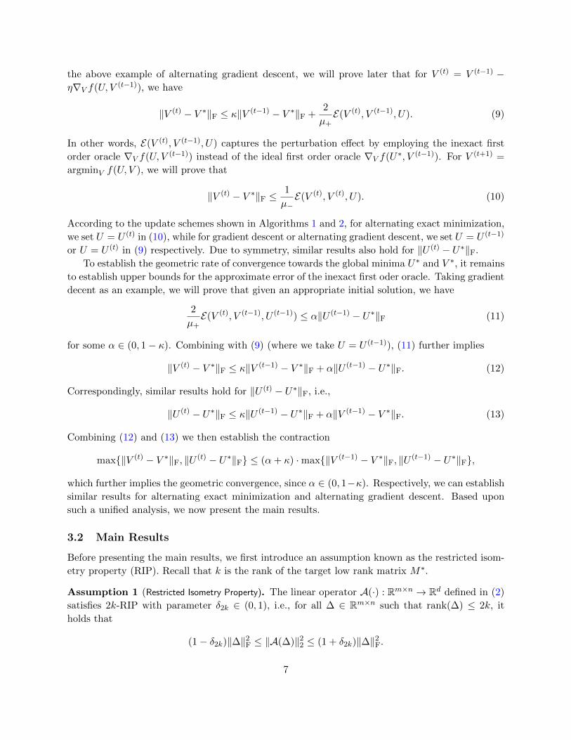
Lemma 3. Suppose that δ2k and U(t)
satisfy
δ2k ≤(1− δ2k)2σk
12ξk(1 + δ2k)σ1and ‖U (t) − U∗(t)‖F ≤
(1− δ2k)σk4ξ(1 + δ2k)σ1
. (16)
Then we have
E(V (t+0.5), V (t+0.5), U(t)
) ≤ (1− δ2k)σk2ξ
‖U (t) − U∗(t)‖F.
The proof of Lemma 3 is provided in Appendix A.2. Lemma 3 shows that the approximation
error of the inexact first order oracle for updating V diminishes with the estimation error of U(t)
,
when U(t)
is sufficiently close to U∗(t)
. The following lemma quantifies the progress of an exact
minimization step using the inexact first order oracle.
Lemma 4. We have
‖V (t+0.5) − V ∗(t)‖F ≤1
1− δ2kE(V (t+0.5), V (t+0.5), U
(t)).
The proof of Lemma 4 is provided in Appendix A.3. Lemma 4 illustrates that the estimation
error of V (t+0.5) diminishes with the approximation error of the inexact first order oracle. The
following lemma characterizes the effect of the renormalization step using QR decomposition, i.e.,
the relationship between V (t+0.5) and V(t+1)
in terms of the estimation error.
Lemma 5. Suppose that V (t+0.5) satisfies
‖V (t+0.5) − V ∗(t)‖F ≤σk4. (17)
Then there exists a factorization of M∗ = U∗(t+1)V∗(t+1)
such that V∗(t+0.5) ∈ Rn×k is an orthonor-
mal matrix, and satisfies
‖V (t+1) − V ∗(t+1)‖F ≤2
σk‖V (t+0.5) − V ∗(t)‖F.
The proof of Lemma 5 is provided in Appendix A.4. The next lemma quantifies the accuracy
of the initialization U(0)
.
Lemma 6. Suppose that δ2k satisfies
δ2k ≤(1− δ2k)2σ4k
192ξ2k(1 + δ2k)2σ41
. (18)
Then there exists a factorization of M∗ = U∗(0)
V ∗(0)> such that U∗(0) ∈ Rm×k is an orthonormal
matrix, and satisfies
‖U (0) − U∗‖F ≤(1− δ2k)σk
4ξ(1 + δ2k)σ1.
10

The proof of Lemma 6 is provided in Appendix A.5. Lemma 6 implies that the initial solution
U(0)
attains a sufficiently small estimation error.
Combining Lemmas 3, 4, and 5, we obtain the following corollary for a complete iteration of
updating V .
Corollary 1. Suppose that δ2k and U(t)
satisfy
δ2k ≤(1− δ2k)2σ4k
192ξ2k(1 + δ2k)2σ41
and ‖U (t) − U∗(t)‖F ≤(1− δ2k)σk
4ξ(1 + δ2k)σ1. (19)
We then have
‖V (t+1) − V ∗(t+1)‖F ≤(1− δ2k)σk
4ξ(1 + δ2k)σ1.
Moreover, we also have
‖V (t+1) − V ∗(t+1)‖F ≤1
ξ‖U (t) − U∗(t)‖F and ‖V (t+0.5) − V ∗(t)‖F ≤
σk2ξ‖U (t) − U∗(t)‖F.
The proof of Corollary 1 is provided in Appendix A.6. Since the alternating exact minimization
algorithm updates U and V in a symmetric manner, we can establish similar results for a complete
iteration of updating U in the next corollary.
Corollary 2. Suppose that δ2k and V(t+1)
satisfy
δ2k ≤(1− δ2k)2σ4k
192ξ2k(1 + δ2k)2σ41
and ‖V (t+1) − V ∗(t+1)‖F ≤(1− δ2k)σk
4ξ(1 + δ2k)σ1. (20)
Then there exists a factorization of M∗ = U∗(t+1)
V ∗(t+1)> such U∗(t+1)
is an orthonormal matrix,
and satisfies
‖U (t+1) − U∗(t+1)‖F ≤(1− δ2k)σk
4ξ(1 + δ2k)σ1.
Moreover, we also have
‖U (t+1) − U∗(t+1)‖F ≤1
ξ‖V (t+1) − V ∗(t+1)‖F and ‖U (t+0.5) − U∗(t+1)‖F ≤
σk2ξ‖V (t+1) − V ∗(t+1)‖F.
The proof of Corollary 2 directly follows Appendix A.6, and is therefore omitted..
We then proceed with the proof of Theorem 1 for alternating exact minimization. Lemma 6
ensures that (19) of Corollary 1 holds for U(0)
. Then Corollary 1 ensures that (20) of Corollary
2 holds for V(1)
. By induction, Corollaries 1 and 2 can be applied recursively for all T iterations.
Thus we obtain
‖V (T ) − V ∗(T )‖F ≤1
ξ‖U (T−1) − U∗(T−1)‖F ≤
1
ξ2‖V (T−1) − V ∗(T−1)‖F
≤ · · · ≤ 1
ξ2T−1‖U (0) − U∗(0)‖F ≤
(1− δ2k)σk4ξ2T (1 + δ2k)σ1
, (21)
11

where the last inequality comes from Lemma 6. Therefore, for a pre-specified accuracy ε, we need
at most
T =
⌈1
2log
((1− δ2k)σk
2ε(1 + δ2k)σ1
)log−1 ξ
⌉(22)
iterations such that
‖V (T ) − V ∗(T )‖F ≤(1− δ2k)σk
4ξ2T (1 + δ2k)σ1≤ ε
2. (23)
Moreover, Corollary 2 implies
‖U (T−0.5) − U∗(T )‖F ≤σk2ξ‖V (T ) − V ∗(T )‖F ≤
(1− δ2k)σ2k8ξ2T+1(1 + δ2k)σ1
,
where the last inequality comes from (21). Therefore, we need at most
T =
⌈1
2log
((1− δ2k)σ2k4ξε(1 + δ2k)
)log−1 ξ
⌉(24)
iterations such that
‖U (T−0.5) − U∗‖F ≤(1− δ2k)σ2k
8ξ2T+1(1 + δ2k)σ1≤ ε
2σ1. (25)
Then combining (23) and (25), we obtain
‖M (T ) −M∗‖ = ‖U (T−0.5)V(T )> − U∗(T )V ∗(T )>‖F
= ‖U (T−0.5)V(T )> − U∗(T )V (T )>
+ U∗(T )V(T )> − U∗(T )V ∗(T )>‖F
≤ ‖V (T )‖2‖U (T−0.5) − U∗(T )‖F + ‖U∗(T )‖2‖V(T ) − V ∗(T )‖F ≤ ε, (26)
where the last inequality comes from ‖V (T )‖2 = 1 (since V(T )
is orthonormal) and ‖U∗‖2 =
‖M∗‖2 = σ1 (since U∗(T )V∗(T )>
= M∗ and V∗(T )
is orthonormal). Thus combining (22) and
(24) with (26), we complete the proof.
4.3 Proof of Theorem 1 (Alternating Gradient Descent)
Proof. Throughout the proof for alternating gradient descent, we define a sufficiently large constant
ξ. Moreover, we assume that at the t-th iteration, there exists a matrix factorization of M∗
M∗ = U∗(t)
V ∗(t)>,
where U∗(t) ∈ Rm×k is an orthonormal matrix. We define the approximation error of the inexact
first order oracle as
E(V (t+0.5), V (t), U(t)
) = ‖∇V F(U(t), V (t))−∇V F(U
∗(t), V (t))‖F.
The first lemma is parallel to Lemma 3 for alternating exact minimization.
12

Lemma 7. Suppose that δ2k, U(t)
, and V (t) satisfy
δ2k ≤(1− δ2k)σk
24ξkσ1, ‖U (t) − U∗(t)‖F ≤
σ2k4ξσ21
, and ‖V (t) − V ∗(t)‖F ≤σ1√k
2. (27)
Then we have
E(V (t+0.5), V (t), U(t)
) ≤ (1 + δ2k)σkξ
‖U (t) − U∗(t)‖F.
The proof of Lemma 7 is provided in Appendix B.1. Lemma 7 illustrates that the approximation
error of the inexact first order oracle diminishes with the estimation error of U(t)
, when U(t)
and
V (t) are sufficiently close to U∗(t)
and V ∗(t).
Lemma 8. Suppose that the step size parameter η satisfies
η =1
1 + δ2k. (28)
Then we have
‖V (t+0.5) − V ∗‖F ≤√δ2k‖V (t) − V ∗‖F +
2
1 + δ2kE(V (t+0.5), V (t), U
(t)).
The proof of Lemma 8 is in Appendix B.2. Lemma 8 characterizes the progress of a gradient
descent step with a pre-specified fixed step size. A more practical option is adaptively selecting η
using the backtracking line search procedure, and similar results can be guaranteed. See Nesterov
[2004] for details. The following lemma characterizes the effect of the renormalization step using
QR decomposition.
Lemma 9. Suppose that V (t+0.5) satisfies
‖V (t+0.5) − V ∗(t)‖F ≤σk4. (29)
Then there exists a factorization of M∗ = U∗(t+1)V∗(t+1)
such that V∗(t+1) ∈ Rn×k is an orthonor-
mal matrix, and
‖V (t+1) − V ∗(t+1)‖F ≤2
σk‖V (t+0.5) − V ∗(t)‖F,
‖U (t) − U∗(t+1)‖F ≤3σ1σk‖V (t+0.5) − V ∗(t)‖F + σ1‖U
(t) − U∗(t)‖F,
The proof of Lemma 9 is provided in Appendix B.3. The next lemma quantifies the accuracy
of the initial solutions.
Lemma 10. Suppose that δ2k satisfies
δ2k ≤σ6k
192ξ2kσ61. (30)
Then we have
‖U (0) − U∗(0)‖F ≤σ2k
4ξσ21and ‖V (0) − V ∗(0)‖F ≤
σ2k2ξσ1
≤ σ1√k
2.
13

The proof of Lemma 10 is in Appendix B.4. Lemma 10 indicates that the initial solutions U(0)
and V (0) attain sufficiently small estimation errors.
Combining Lemmas 7, 8, 5, , we obtain the following corollary for a complete iteration of
updating V .
Corollary 3. Suppose that δ2k, U(t)
, and V (t) satisfy
δ2k ≤σ6k
192ξ2kσ61, ‖U (t) − U∗(t)‖F ≤
σ2k4ξσ21
, and ‖V (t) − V ∗(t)‖F ≤σ2k
2ξσ1. (31)
We then have
‖V (t+1) − V ∗(t+1)‖F ≤σ2k
4ξσ21and ‖U (t) − U∗(t+1)‖F ≤
σ2k2ξσ1
.
Moreover, we have
‖V (t+0.5) − V ∗(t)‖F ≤√δ2k‖V (t) − V ∗(t)‖F +
2σkξ‖U (t) − U∗(t)‖F, (32)
‖V (t+1) − V ∗(t+1)‖F ≤2√δ2kσk‖V (t) − V ∗(t)‖F +
4
ξ‖U (t) − U∗(t)‖F, (33)
‖U (t) − U∗(t+1)‖F ≤3σ1√δ2k
σk‖V (t) − V ∗(t)‖F +
(6
ξ+ 1
)σ1‖U
(t) − U∗(t)‖F. (34)
The proof of Corollary 3 is provided in Appendix B.5. Since the alternating gradient descent
algorithm updates U and V in a symmetric manner, we can establish similar results for a complete
iteration of updating U in the next corollary.
Corollary 4. Suppose that δ2k, V(t+1)
, and U (t) satisfy
δ2k ≤σ6k
192ξ2kσ61, ‖V (t+1) − V ∗(t+1)‖F ≤
σ2k4ξσ21
, and ‖U (t) − U∗(t+1)‖F ≤σ2k
2ξσ1. (35)
We then have
‖U (t+1) − U∗(t+1)‖F ≤σ2k
4ξσ21and ‖V (t+1) − V ∗(t+1)‖F ≤
σ2k2ξσ1
.
Moreover, we have
‖U (t+0.5) − U∗(t+1)‖F ≤√δ2k‖U (t) − U∗(t+1)‖F +
2σkξ‖V (t+1) − V ∗(t+1)‖F, (36)
‖U (t+1) − U∗(t+1)‖F ≤2√δ2kσk‖U (t) − U∗(t+1)‖F +
4
ξ‖V (t+1) − V ∗(t+1)‖F, (37)
‖V (t+1) − V ∗(t+1)‖F ≤3σ1√δ2k
σk‖U (t) − U∗(t+1)‖F +
(6
ξ+ 1
)σ1‖V
(t+1) − V ∗(t+1)‖F. (38)
14

The proof of Corollary 4 directly follows Appendix B.5, and is therefore omitted..
Now we proceed with the proof of Theorem 1 for alternating gradient descent. Recall that
Lemma 10 ensures that (31) of Corollary 3 holds for U(0)
and V (0). Then Corollary 3 ensures
that (35) of Corollary 4 holds for U (0) and V(1)
. By induction, Corollaries 1 and 2 can be applied
recursively for all T iterations. For notational simplicity, we write (32)-(38) as
‖V (t+0.5) − V ∗(t)‖F ≤ α1‖V (t) − V ∗(t)‖F + γ1σ1‖U(t) − U∗(t)‖F, (39)
σ1‖V(t+1) − V ∗(t+1)‖F ≤ α2‖V (t) − V ∗(t)‖F + γ2σ1‖U
(t) − U∗(t)‖F, (40)
‖U (t+0.5) − U∗(t+1)‖F ≤ α3‖U (t) − U∗(t+1)‖F + γ3σ1‖V(t+1) − V ∗(t+1)‖F, (41)
σ1‖U(t+1) − U∗(t+1)‖F ≤ α4‖U (t) − U∗(t+1)‖F + γ4σ1‖V
(t+1) − V ∗(t+1)‖F, (42)
‖U (t) − U∗(t+1)‖F ≤ α5‖V (t) − V ∗(t)‖F + γ5σ1‖U(t) − U∗(t)‖F, (43)
‖V (t+1) − V ∗(t+1)‖F ≤ α6‖U (t) − U∗(t+1)‖F + γ6σ1‖V(t+1) − V ∗(t+1)‖F. (44)
Note that we have γ5, γ6 ∈ (1, 2), but α1,...,α6, γ1,..., and γ4 can be sufficiently small as long as ξ
is sufficiently large. We then have
‖U (t+1) − U∗(t+2)‖F(i)
≤α5‖V (t+1) − V ∗(t+1)‖F + γ5σ1‖U(t+1) − U∗(t+1)‖F
(ii)
≤ α5α6‖U (t) − U∗(t+1)‖F + α5γ6σ1‖V(t+1) − V ∗(t+1)‖F + γ5σ1‖U
(t+1) − U∗(t+1)‖F(iii)
≤ (α5α6 + γ5α4)‖U (t) − U∗(t+1)‖F + (γ5γ4σ1 + α5γ6)σ1‖V(t+1) − V ∗(t+1)‖F
(iv)
≤ (α5α6 + γ5α4)‖U (t) − U∗(t+1)‖F + (γ5γ4σ1 + α5γ6)α2‖V (t) − V ∗(t)‖F
+ (γ5γ4σ1 + α5γ6)γ2σ1‖U(t) − U∗(t)‖F, (45)
where (i) comes from (43), (ii) comes from (44), (iii) comes from (42), and (iv) comes from (40).
Similarly, we can obtain
‖V (t+1) − V ∗(t+1)‖F ≤ α6‖U (t) − U∗(t+1)‖F + γ6α2‖V (t) − V ∗(t)‖F
+ γ6γ2σ1‖U(t) − U∗(t)‖F, (46)
σ1‖U(t+1) − U∗(t+1)‖F ≤ α4‖U (t) − U∗(t+1)‖F + γ4α2‖V (t) − V ∗(t)‖F
+ γ4γ2σ1‖U(t) − U∗(t)‖F (47)
‖U (t+0.5) − U∗(t+1)‖F ≤ α3‖U (t) − U∗(t+1)‖F + γ3α2‖V (t) − V ∗(t)‖F
+ γ3γ2σ1‖U(t) − U∗(t)‖F. (48)
For simplicity, we define
φV (t+1) = ‖V (t+1) − V ∗(t+1)‖F, φV (t+0.5) = ‖V (t+0.5) − V ∗(t)‖F, φV (t+1) = σ1‖V(t+1) − V ∗(t+1)‖F,
φU(t+1) = ‖U (t+1) − U∗(t+2)‖F, φU(t+0.5) = ‖U (t+0.5) − U∗(t+1)‖F, φU(t+1) = σ1‖U(t+1) − U∗(t+1)‖F.
15

Then combining (39), (40) with (45)–(48), we obtain
maxφV (t+1) , φV (t+0.5) , φ
V(t+1) , φU(t+1) , φU(t+0.5) , φ
U(t+1)
≤ βmax
φV (t) , φU(t) , φ
U(t)
, (49)
where β is a contraction coefficient defined as
β = maxα5α6 + γ5α4, α6, α4, α3+ maxα1, α2, (γ5γ4σ1 + α5γ6), γ6α2, γ4α2, γ3α2+ maxγ1, γ2, (γ5γ4σ1 + α5γ6)γ2, γ6γ2, γ4γ2, γ3γ2.
Then we can choose ξ as a sufficiently large constant such that β < 1. By recursively applying (49)
for t = 0, ..., T , we obtain
maxφV (T ) , φV (T−0.5) , φ
V(T ) , φU(T ) , φU(T−0.5) , φ
U(T )
≤ βmax
φV (T−1) , φU(T−1) , φ
U(T−1)
≤ β2 max
φV (T−2) , φU(T−2) , φ
U(T−2)
≤ ... ≤ βT max
φV (0) , φU(0) , φ
U(0)
.
By Corollary 3, we obtain
‖U (0) − U∗(1)‖F ≤3σ1√δ2k
σk‖V (0) − V ∗(0)‖F +
(6
ξ+ 1
)σ1‖U
(0) − U∗(0)‖F
(i)
≤ 3σ1σk·
σ3k12ξσ31
·σ2k
2ξσ1+
(6
ξ+ 1
)σ2k
4ξσ1
(ii)=
σ4k8ξ2σ31
+3σ2k
2ξ2σ1+
σ2k4ξσ1
(iii)
≤σ2k
2ξσ1, (50)
where (i) and (ii) come from Lemma 10, and (iii) comes from the definition of ξ and σ1 ≥ σk.
Combining (50) with Lemma 10, we have
φV (0) , φU(0) , φ
U(0)
≤ max
σ2k2ξσ1
,σ2k
4ξσ21
.
Then we need at most
T =
⌈log
(max
σ2kξσ1
,σ2k
2ξσ21,σ2kξ,σ2k
2ξσ1
· 1
ε
)log−1(β−1)
⌉iterations such that
‖V (T ) − V ∗‖F ≤ βT max σ2k
2ξσ1,σ2k
4ξσ21
≤ ε
2and ‖U (T ) − U∗‖F ≤ βT max
σ2k2ξσ1
,σ2k
4ξσ21
≤ ε
2σ1.
We then follow similar lines to (26) in §4.2, and show ‖M (T ) −M∗‖F ≤ ε, which completes the
proof.
4.4 Proof of Theorem 1 (Gradient Descent)
Proof. The convergence analysis of the gradient descent algorithm is similar to that of the alter-
nating gradient descent. The only difference is that for updating U , the gradient descent algorithm
employs V = V(t)
instead of V = V(t+1)
to calculate the gradient at U = U (t). Then everything
else directly follows §4.3, and is therefore omitted..
16

5 Extensions to Matrix Completion
We then extend our methodology and theory to matrix completion problems. Let M∗ ∈ Rm×nbe the unknown low rank matrix of interest. We observe a subset of the entries of M∗, namely,
W ⊆ 1, . . . ,m × 1, . . . , n. We assume that W is drawn uniformly at random, i.e., M∗i,j is
observed independently with probability ρ ∈ (0, 1]. To exactly recover M∗, a common assumption
is the incoherence of M∗, which will be specified later. A popular approach for recovering M∗ is
to solve the following convex optimization problem
minM∈Rm×n
‖M‖∗ subject to PW(M∗) = PW(M), (51)
where PW(M) : Rm×n → Rm×n is an operator defined as
[PW(M)]ij =
Mij if (i, j) ∈ W,
0 otherwise.
Similar to matrix sensing, existing algorithms for solving (51) are computationally inefficient.
Hence, in practice we usually consider the following nonconvex optimization problem
minU∈Rm×k,V ∈Rn×k
FW(U, V ), where FW(U, V ) =1
2‖PW(M∗)− PW(UV >)‖2F. (52)
Similar to matrix sensing, (52) can also be efficiently solved by gradient-based algorithms illustrated
in Algorithm 2. For the convenience of later convergence analysis, we partition the observation set
W into 2T+1 subsetsW0,...,W2T by Algorithm 4. However, in practice we do not need the partition
scheme, i.e., we simply set W0 = · · · =W2T =W.
Before we present the convergence analysis, we first introduce an assumption known as the
incoherence property.
Assumption 2 (Incoherence Property). The target rank k matrix M∗ is incoherent with parameter
µ, i.e., given the rank k singular value decomposition of M∗ = U∗Σ∗V
∗>, we have
maxi‖U∗i∗‖2 ≤ µ
√k
mand max
j‖V ∗j∗‖2 ≤ µ
√k
n.
Roughly speaking, the incoherence assumption guarantees that each entry of M∗ contains sim-
ilar amount of information, which makes it feasible to complete M∗ when its entries are missing
uniformly at random. The following theorem establishes the iteration complexity and the estima-
tion error under the Frobenius norm.
Theorem 2. Suppose that there exists a universal constant C4 such that ρ satisfies
ρ ≥ C4µ2k3 log n log(1/ε)
m, (53)
where ε is the pre-specified precision. Then there exist an η and universal constants C5 and C6
such that for any T ≥ C5 log(C6/ε), we have ‖M (T ) −M‖F ≤ ε with high probability.
17

Algorithm 2 A family of nonconvex optimization algorithms for matrix completion. The in-
coherence factorization algorithm IF(·) is illustrated in Algorithm 3, and the partition algorithm
Partition(·), which is proposed by Hardt and Wootters [2014], is provided in Algorithm 4 of Ap-
pendix C for the sake of completeness. The initialization procedures INTU (·) and INTU (·) are
provided in Algorithm 5 and Algorithm 6 of Appendix D for the sake of completeness. Here FW(·)is defined in (52).
Input: PW(M∗)
Parameter: Step size η, Total number of iterations T
(Wt2Tt=0, ρ)← Partition(W), PW0(M)← PW0(M∗), and Mij ← 0 for all (i, j) /∈ W0
(U(0), V (0))← INTU (M), (V
(0), U (0))← INTV (M)
For: t = 0, ...., T − 1
Alternating Exact Minimization : V (t+0.5) ← argminV FW2t+1(U(t), V )
(V(t+1)
, R(t+0.5)
V)← IF(V (t+0.5))
Alternating Gradient Descent : V (t+0.5) ← V (t) − η∇V FW2t+1(U(t), V (t))
(V(t+1)
, R(t+0.5)
V)← IF(V (t+0.5)), U (t) ← U
(t)R
(t+0.5)>V
Gradient Descent : V (t+0.5) ← V (t) − η∇V FW2t+1(U(t), V (t))
(V(t+1)
, R(t+0.5)
V)← IF(V (t+0.5)), U (t+1) ← U
(t)R
(t+0.5)>V
Updating V .
Alternating Exact Minimization : U (t+0.5) ← argminU FW2t+2(U, V(t+1)
)
(U(t+1)
, R(t+0.5)
U)← IF(U (t+0.5))
Alternating Gradient Descent : U (t+0.5) ← U (t) − η∇UFW2t+2(U (t), V(t+1)
)
(U(t+1)
, R(t+0.5)
U)← IF(U (t+0.5)), V (t+1) ← V
(t+1)R
(t+0.5)>U
Gradient Descent : U (t+0.5) ← U (t) − η∇UFW2t+2(U (t), V(t)
)
(U(t+1)
, R(t+0.5)
U)← IF(U (t+0.5)), V (t+1) ← V
(t)R
(t+0.5)>U
Updating U .
End for
Output: M (T ) ← U (T−0.5)V(T )>
(for gradient descent we use U(T )V (T )>)
Algorithm 3 The incoherence factorization algorithm for matrix completion. It guarantees that
the solutions satisfy the incoherence condition throughout all iterations.
Input: W in
r ← Number of rows of W in
Parameter: Incoherence parameter µ
(Win, Rin
W)← QR(W in)
W ← argminW
‖W −W in‖2F subject to maxj‖Wj∗‖2 ≤ µ
√k/r
(Wout, Rtmp
W)← QR(W out)
RoutW
= Wout>
W in
Output: Wout, Rout
W
18
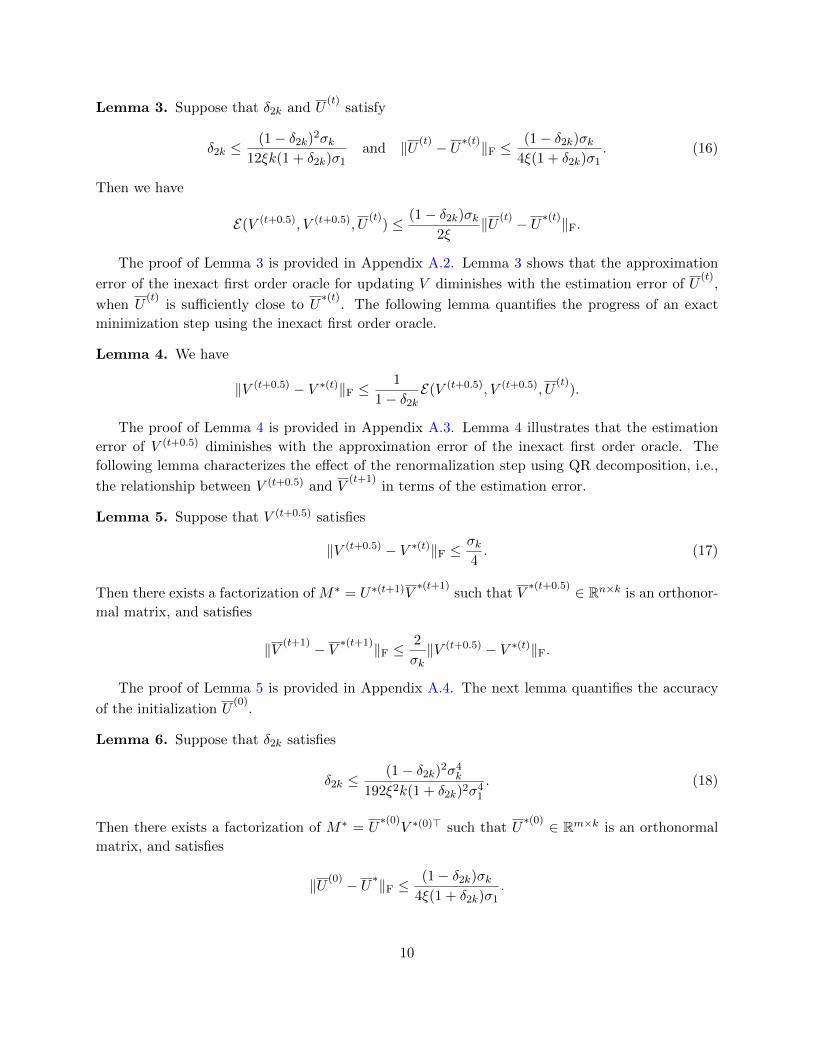
The proof of Theorem 2 is provided in §F.1, §F.2, and §F.3. Theorem 2 implies that all
three nonconvex optimization algorithms converge to the global optimum at a geometric rate.
Furthermore, our results indicate that the completion of the true low rank matrix M∗ up to ε-
accuracy requires the entry observation probability ρ to satisfy
ρ = Ω(µ2k3 log n log(1/ε)/m). (54)
This result matches the result established by Hardt [2014], which is the state-of-the-art result for
alternating minimization. Moreover, our analysis covers three nonconvex optimization algorithms.
In fact, the sample complexity in (54) depends on a polynomial of σmax(M∗)σmin(M∗)
, which is a constant
since in this paper we assume that σmax(M∗) and σmin(M∗) are constants. If we allow σmax(M∗)σmin(M∗)
to
increase, we can replace the QR decomposition in Algorithm 3 with the smooth QR decomposition
proposed by Hardt and Wootters [2014] and achieve a dependency of log(σmax(M∗)σmin(M∗)
)on the condi-
tion number with a more involved proof. See more details in Hardt and Wootters [2014]. However,
in this paper, our primary focus is on the dependency on k, n and m, rather than optimizing over
the dependency on condition number.
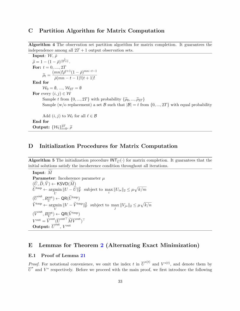
6 Numerical Experiments
We present numerical experiments to support our theoretical analysis. We first consider a matrix
sensing problem with m = 30, n = 40, and k = 5. We vary d from 300 to 900. Each entry of Ai’s are
independent sampled from N(0, 1). We then generate M = UV >, where U ∈ Rm×k and V ∈ Rn×kare two matrices with all their entries independently sampled from N(0, 1/k). We then generate d
measurements by bi = 〈Ai,M〉 for i = 1, ..., d. Figure 1 illustrates the empirical performance of the
alternating exact minimization and alternating gradient descent algorithms for a single realization.
The step size for the alternating gradient descent algorithm is determined by the backtracking line
search procedure. We see that both algorithms attain linear rate of convergence for d = 600 and
d = 900. Both algorithms fail for d = 300, because d = 300 is below the minimum requirement of
sample complexity for the exact matrix recovery.
We then consider a matrix completion problem with m = 1000, n = 50, and k = 5. We vary ρ
from 0.025 to 0.1. We then generate M = UV >, where U ∈ Rm×k and V ∈ Rn×k are two matrices
with all their entries independently sampled from N(0, 1/k). The observation set is generated
uniformly at random with probability ρ. Figure 2 illustrates the empirical performance of the
alternating exact minimization and alternating gradient descent algorithms for a single realization.
The step size for the alternating gradient descent algorithm is determined by the backtracking line
search procedure. We see that both algorithms attain linear rate of convergence for ρ = 0.05 and
ρ = 0.1. Both algorithms fail for ρ = 0.025, because the entry observation probability is below the
minimum requirement of sample complexity for the exact matrix recovery.
7 Conclusion
In this paper, we propose a generic analysis for characterizing the convergence properties of noncon-
vex optimization algorithms. By exploiting the inexact first order oracle, we prove that a broad class
19

Numer of Iterations0 10 20 30 40
Estimation Error
10-6
10-4
10-2
100
102
d=300d=600d=900
(a) Alternating Exact Minimization Algorithm
Number of Iterations0 20 40 60 80
Estaimation Error
10-6
10-4
10-2
100
102
d=300d=600d=900
(b) Alternating Gradient Descent Algorithm
Figure 1: Two illustrative examples for matrix sensing. The vertical axis corresponds to estimation
error ‖M (t)−M‖F. The horizontal axis corresponds to numbers of iterations. Both the alternating
exact minimization and alternating gradient descent algorithms attain linear rate of convergence
for d = 600 and d = 900. But both algorithms fail for d = 300, because the sample size is not large
enough to guarantee proper initial solutions.
of nonconvex optimization algorithms converge geometrically to the global optimum and exactly
recover the true low rank matrices under suitable conditions.
A Lemmas for Theorem 1 (Alternating Exact Minimization)
A.1 Proof of Lemma 1
Proof. For notational convenience, we omit the index t in U∗(t)
and V ∗(t), and denote them by U∗
and V ∗ respectively. Then we define two nk × nk matrices
S(t) =
S(t)11 · · · S
(t)1k
.... . .
...
S(t)k1 · · · S
(t)kk
with S(t)pq =
d∑i=1
AiU(t)∗pU
(t)>∗q A>i ,
G(t) =
G
(t)11 · · · G
(t)1k
.... . .
...
G(t)k1 · · · G
(t)kk
with G(t)pq =
d∑i=1
AiU∗∗pU
∗>∗q A
>i
for 1 ≤ p, q ≤ k. Note that S(t) and G(t) are essentially the partial Hessian matrices ∇2V F(U
(t), V )
and ∇2V F(U
∗, V ) for a vectorized V , i.e., vec(V ) ∈ Rnk. Before we proceed with the main proof,
we first introduce the following lemma.
20

Number of Iterations0 20 40 60 80 100
Estimation Error
10-8
10-6
10-4
10-2
100
102
7; = 0:0257; = 0:0257; = 0:025
(a) Alternating Exact Minimization Algorithm
Number of Iterations0 10 20 30 40 50
Estimation Error
10-8
10-6
10-4
10-2
100
102
7; = 0:0257; = 0:057; = 0:1
(b) Alternating Gradient Descent Algorithm
Figure 2: Two illustrative examples for matrix completion. The vertical axis corresponds to esti-
mation error ‖M (t) −M‖F. The horizontal axis corresponds to numbers of iterations. Both the
alternating exact minimization and alternating gradient descent algorithms attain linear rate of
convergence for ρ = 0.05 and ρ = 0.1. But both algorithms fail for ρ = 0.025, because the entry
observation probability is not large enough to guarantee proper initial solutions.
Lemma 11. Suppose that A(·) satisfies 2k-RIP with parameter δ2k. We then have
1 + δ2k ≥ σmax(S(t)) ≥ σmin(S(t)) ≥ 1− δ2k.
The proof of Lemma 11 is provided in Appendix A.7. Note that Lemma 11 is also applicable
G(t), since G(t) shares the same structure with S(t).
We then proceed with the proof of Lemma 1. Given a fixed U , F(U, V ) is a quadratic function
of V . Therefore we have
F(U, V ′) = F(U, V ) + 〈∇V F(U, V ), V ′ − V 〉+ 〈vec(V ′)− vec(V ),∇2V F (U, V )
(vec(V ′)− vec(V )
)〉,
which further implies implies
F(U, V ′)−F(U, V )− 〈∇V (U, V ), V ′ − V 〉 ≤ σmax(∇2V F (U, V ))‖V ′ − V ‖2F
F(U, V ′)−F(U, V )− 〈∇V (U, V ), V ′ − V 〉 ≥ σmin(∇2V F (U, V ))‖V ′ − V ‖2F.
Then we can verify that∇2V F (U, V ) also shares the same structure with S(t). Thus applying Lemma
11 to the above two inequalities, we complete the proof.
21

A.2 Proof of Lemma 3
Proof. For notational convenience, we omit the index t in U∗(t)
and V ∗(t), and denote them by U∗
and V ∗ respectively. We define two nk × nk matrices
J (t) =
J(t)11 · · · J
(t)1k
.... . .
...
J(t)k1 · · · J
(t)kk
with J (t)pq =
d∑i=1
AiU(t)∗pU
∗>∗q A
>i ,
K(t) =
K
(t)11 · · · K
(t)1k
.... . .
...
K(t)k1 · · · K
(t)kk
with K(t)pq = U
(t)>∗p U
∗∗qIn
for 1 ≤ p, q ≤ k. Before we proceed with the main proof, we first introduce the following lemmas.
Lemma 12. Suppose that A(·) satisfies 2k-RIP with parameter δ2k. We then have
‖S(t)K(t) − J (t)‖2 ≤ 3δ2k√k‖U (t) − U∗‖F.
The proof of Lemma 12 is provided in Appendix A.8. Note that Lemma 12 is also applicable
to G(t)K(t) − J (t), since G(t) and S(t) share the same structure.
Lemma 13. Given F ∈ Rk×k, we define a nk × nk matrix
F =
F11In · · · F1kIn...
. . ....
Fk1In · · · FkkIn
.For any V ∈ Rn×k, let v = vec(V ) ∈ Rnk, then we have ‖Fv‖2 = ‖FV >‖F.
Proof. By linear algebra, we have
[FV ]ij = F>i∗Vj∗ =
k∑`=1
Fi`Vj` =k∑`=1
Fi`I>∗`V∗`,
which completes the proof.
We then proceed with the proof of Lemma 3. Since bi = tr(V ∗>AiU∗), then we rewrite F(U, V )
as
F(U, V ) =1
2
d∑i=1
(tr(V >AiU)− bi
)2=
1
2
d∑i=1
( k∑j=1
V >j∗AiU∗j −k∑j=1
V ∗>j∗ AiU∗∗j
)2
.
For notational simplicity, we define v = vec(V ). Since V (t+0.5) minimizes F(U(t), V ), we have
vec(∇UF(U
(t), V (t+0.5))
)= S(t)v(t+0.5) − J (t)v∗ = 0.
22

Solving the above system of equations, we obtain
v(t+0.5) = (S(t))−1J (t)v∗. (55)
Meanwhile, we have
vec(∇V F(U∗, V (t+0.5))) = G(t)v(t+0.5) −G(t)v∗
= G(t)(S(t))−1J (t)v∗ −G(t)v∗ = G(t)((S(t))−1J (t) − Ink
)v∗, (56)
where the second equality come from (55). By triangle inequality, (56) further implies
‖((S(t))−1J (t) − Ink)v∗‖2 ≤ ‖(K(t) − Ink)v∗‖2 + ‖(S(t))−1(J (t) − S(t)K(t))v∗‖2
≤ ‖(U (t)>U∗ − Ik)V ∗>‖F + ‖(S(t))−1‖2‖(J (t) − S(t)K(t))v∗‖2
≤ ‖U (t)>U∗ − Ik‖F‖V ∗‖2 + ‖(S(t))−1‖2‖(J (t) − S(t)K(t))v∗‖2, (57)
where the second inequality comes from Lemma 13. Plugging (57) into (56), we have
‖vec(∇V F(U∗, V (t+0.5)))‖2 ≤ ‖G(t)‖2‖((S(t))−1J (t) − Ink)v∗‖2
(i)
≤(1 + δ2k)(σ1‖U(t)>
U∗ − Ik‖2 + ‖(S(t))−1‖2‖S(t)K(t) − J (t)‖2σ1
√k)
(ii)
≤ (1 + δ2k)σ1
(‖(U (t) − U∗)>(U
(t) − U∗)‖F +3δ2kk
1− δ2k‖U (t) − U∗‖F
)(iii)
≤ (1 + δ2k)σ1
(‖U (t) − U∗‖2F +
3δ2kk
1− δ2k‖U (t) − U∗‖F
) (iv)
≤ (1− δ2k)σk2ξ
‖U∗ − U (t)‖F,
where (i) comes from Lemma 11 and ‖V ∗‖2 = ‖M∗‖ = σ1 and ‖V ∗‖F = ‖v∗‖2 ≤ σ1√k, (ii) comes
from Lemmas 11 and 12, (iii) from Cauchy-Schwartz inequality, and (iv) comes from (16). Since
we have ∇V F(U(t), V (t+0.5)) = 0, we further btain
E(V (t+0.5), V (t+0.5), U(t)
) ≤ (1− δ2k)σk2ξ
‖U∗ − U (t)‖F,
which completes the proof.
A.3 Proof of Lemma 4
Proof. For notational convenience, we omit the index t in U∗(t)
and V ∗(t), and denote them by U∗
and V ∗ respectively. By the strong convexity of F(U∗, ·), we have
F(U∗, V ∗)− 1− δ2k
2‖V (t+0.5) − V ∗‖2F ≥ F(U
∗, V (t+0.5))
+ 〈∇V F(U∗, V (t+0.5)), V ∗ − V (t+0.5)〉. (58)
By the strong convexity of F(U∗, ·) again, we have
F(U∗, V (t+0.5)) ≥ F(U
∗, V ∗) + 〈∇V F(U
∗, V ∗), V (t+0.5) − V (t+0.5)〉+
1− δ2k2‖V (t+0.5) − V ∗‖2F
≥ F(U∗, V ∗) +
1− δ2k2‖V (t+0.5) − V ∗‖2F, (59)
23

where the last inequality comes from the optimality condition of V ∗ = argminV F(U∗, V ), i.e.
〈∇V F(U∗, V ∗), V (t+0.5) − V ∗〉 ≥ 0.
Meanwhile, since V (t+0.5) minimizes F(U(t), ·), we have the optimality condition
〈∇V F(U(t), V (t+0.5)), V ∗ − V (t+0.5)〉 ≥ 0,
which further implies
〈∇V F(U∗, V (t+0.5)), V ∗ − V (t+0.5)〉
≥ 〈∇V F(U∗, V (t+0.5))−∇V F(U
(t), V (t+0.5)), V ∗ − V (t+0.5)〉. (60)
Combining (58) and (59) with (60), we obtain
‖V (t+0.5) − V ∗‖2 ≤1
1− δ2kE(V (t+0.5), V (t+0.5), U
(t)),
which completes the proof.
A.4 Proof of Lemma 5
Proof. Before we proceed with the proof, we first introduce the following lemma.
Lemma 14. Suppose that A∗ ∈ Rn×k is a rank k matrix. Let E ∈ Rn×k satisfy ‖E‖2‖A∗†‖2 < 1.
Then given a QR decomposition (A∗ + E) = QR, there exists a factorization of A∗ = Q∗O∗ such
that Q∗ ∈ Rn×k is an orthonormal matrix, and satisfies
‖Q−Q∗‖F ≤√
2‖A∗†‖2‖E‖F1− ‖E‖2‖A∗†‖2
.
The proof of Lemma 14 is provided in Stewart et al. [1990], therefore omitted.
We then proceed with the proof of Lemma 5. We consider A∗ = V ∗(t) and E = V (t+0.5) − V ∗(t)in Lemma 14 respectively. We can verify that
‖V (t+0.5) − V ∗(t)‖2‖V ∗(t)†‖2 ≤‖V (t+0.5) − V ∗(t)‖F
σk≤ 1
4.
Then there exists a V ∗(t) = V∗(t+1)
O∗ such that V∗(t+1)
is an orthonormal matrix, and satisfies
‖V ∗(t+0.5) − V ∗(t+1)‖F ≤ 2‖V ∗(t)†‖2‖V (t+0.5) − V ∗(t)‖F ≤2
σk‖V (t+0.5) − V ∗(t)‖F.
24

A.5 Proof of Lemma 6
Proof. Before we proceed with the main proof, we first introduce the following lemma.
Lemma 15. Let b = A(M∗) + ε, M is a rank-k matrix, and A is a linear measurement operator
that satisfies 2k-RIP with constant δ2k < 1/3. Let X(t+1) be the (t + 1)-th step iterate of SVP,
then we have
‖A(X(t+1))− b‖22 ≤ ‖A(M∗)− b‖22 + 2δ2k‖A(X(t))− b‖22
The proof of Lemma 15 is provided in Jain et al. [2010], therefore omitted. We then explain
the implication of Lemma 15. Jain et al. [2010] show that X(t+1) is obtained by taking a projected
gradient iteration over X(t) using step size 11+δ2k
. Then taking X(t) = 0, we have
X(t+1) =U
(0)Σ(0)V
(0)>
1 + δ2k.
Then Lemma 15 implies ∥∥∥∥A(U (0)Σ(0)V
(0)>
1 + δ2k−M∗
)∥∥∥∥22
≤ 4δ2k‖A(M∗)‖22. (61)
Since A(·) satisfies 2k-RIP, then (61) further implies∥∥∥∥U (0)Σ(0)V
(0)>
1 + δ2k−M∗
∥∥∥∥2
F
≤ 4δ2k(1 + 3δ2k)‖M∗‖2F. (62)
We then project each column of M∗ into the subspace spanned by U (0)∗i ki=1, and obtain
‖U (0)U
(0)>M∗ −M∗‖2F ≤ 6δ2k‖M∗‖2F.
Let U(0)⊥ denote the orthonormal complement of U
(0), i.e.,
U(0)>⊥ U
(0)⊥ = In−k and U
(0)>⊥ U
(0)= 0.
Then given a compact singular value decomposition of M∗ = U∗D∗V ∗>, we have
6δ2kkσ21
σ2k≥ ‖(U (0)
U(0)> − In)U∗‖2F = ‖U (0)>
⊥ U∗‖2F.
Thus Lemma 2 guarantees that for O∗ = argminO>O=Ik‖U (0) − U∗O‖F, we have
‖U (0) − U∗O∗‖F ≤√
2‖U (0)>⊥ U∗‖F ≤ 2
√3δ2kk ·
σ1σk.
We define U∗(0)
= U∗O∗. Then combining the above inequality with (18), we have
‖U (0) − U∗(0)‖F ≤(1− δ2k)σk
4ξ(1 + δ2k)σ1.
Meanwhile, we define V ∗(0) = V ∗D∗O∗. Then we have U∗(0)
V ∗(0)> = U∗OO∗>D∗V ∗ = M∗.
25

A.6 Proof of Corollary 1
Proof. Since (19) ensures that (16) of Lemma 3 holds, then we have
‖V (t+0.5) − V ∗(t)‖F ≤1
1− δ2kE(V (t+0.5), V (t+0.5), U
(t))(i)
≤ 1
1− δ2k· (1− δ2k)σk
2ξ‖U (t) − U∗(t)‖F
(ii)
≤ 1
1− δ2k· (1− δ2k)σk
2ξ· (1− δ2k)σk
4ξ(1 + δ2k)σ1≤(
(1− δ2k)σk8ξ2(1 + δ2k)σ1
)σk
(iii)
≤ σk4, (63)
where (i) comes from Lemma 4, (ii) comes from (19), and (iii) comes from the definition of ξ and
σk ≤ σ1. Since (63) ensures that (17) of Lemma 5 holds for V (t+0.5), then we obtain
‖V (t+1) − V ∗(t+1)‖F ≤2
σk‖V (t+0.5) − V ∗(t)‖F
(i)
≤ 1
ξ‖U (t) − U∗(t)‖F
(ii)
≤ (1− δ2k)σk4ξ(1 + δ2k)σ1
, (64)
where (i) comes from (63), and (ii) comes from the definition of ξ and (19).
A.7 Proof of Lemma 11
Proof. We consider an arbitrary W ∈ Rn×k such that ‖W‖F = 1. Let w = vec(W ). Then we have
w>Bw =k∑
p,q=1
W>∗pS(t)pqW∗p =
k∑p,q=1
W>∗p
( d∑i=1
AiU(t)∗pU
(t)>∗q A>i
)W∗q
=d∑i=1
( k∑p=1
W>∗pAiU(t)∗p
)( k∑q=1
W>∗qAiU(t)∗q
)=
n∑i=1
tr(W>AiU(t)
)2 = ‖A(U(t)W>)‖22.
Since A(·) satisfies 2k-RIP, then we have
‖A(U(t)W>)‖22 ≥ (1− δ2k)‖U
(t)W>‖F = (1− δ2k)‖W‖F = 1− δ2k,
‖A(U(t)W>)‖22 ≤ (1 + δ2k)‖U
(t)W>‖F = (1 + δ2k)‖W‖F = 1 + δ2k.
Since W is arbitrary, then we have
σmin(S(t)) = min‖w‖2=1
w>S(t)w ≥ 1− δ2k and σmax(S(t)) = max‖w‖2=1
w>S(t)w ≤ 1 + δ2k.
A.8 Proof of Lemma 12
Proof. For notational convenience, we omit the index t in U∗(t)
and V ∗(t), and denote them by
U∗
and V ∗ respectively. Before we proceed with the main proof, we first introduce the following
lemma.
Lemma 16. Suppose A(·) satisfies 2k-RIP. For any U, U ′ ∈ Rm×k and V, V ′ ∈ Rn×k, we have
|〈A(UV >),A(U ′V ′>)〉 − 〈U>U ′, V >V ′〉| ≤ 3δ2k‖UV >‖F · ‖U ′V ′>‖F.
26

The proof of Lemma 16 is provided in Jain et al. [2013], and hence omitted.
We now proceed with the proof of Lemma 12. We consider arbitrary W,Z ∈ Rn×k such that
‖W‖F = ‖Z‖F = 1. Let w = vec(W ) and z = vec(Z). Then we have
w>(S(t)K(t) − J (t))z =k∑
p,q=1
W>∗p[S(t)K(t) − J (t)]pqZ∗q.
We consider a decomposition
[S(t)K(t) − J (t)]pq =k∑`=1
S(t)p` K
(t)`q − J
(t)pq =
k∑`=1
S(t)p` U
(t)>∗` U
∗∗qIn − J (t)
pq
=k∑`=1
U∗>∗q U
(t)∗`
d∑i=1
AiU(t)∗pU
(t)∗`A
>i − J (t)
pq =k∑`=1
AiU∗>∗q U
(t)∗`
d∑i=1
U(t)∗pU
(t)∗`A
>i −
d∑i=1
AiU(t)∗pU
∗∗qA
>i
=d∑i=1
AiU(t)∗pU
∗∗q(U
(t)U
(t)> − In)A>i .
which further implies
w>(S(t)K(t) − J (t))z =∑p,q
W>∗p
( d∑i=1
AiU(t)∗pU
∗∗q(U
(t)U
(t)> − Im)A>i
)Z∗q
=d∑i=1
∑p,q
W>∗pAiU(t)∗pU
∗∗q(U
(t)U
(t)> − Im)A>i Z∗q
=d∑i=1
tr(W>AiU(t)
) tr(Z>Ai(U
(t)U
(t)> − Im)U∗). (65)
Since A(·) satisfies 2k-RIP, then by Lemma 16, we obtain
w>(S(t)K(t) − J (t))z ≤ tr(U∗(U
(t)U
(t)> − Im)U(t)W>Z
)+ 3δ2k‖U
(t)W>‖F‖(U
(t)U
(t)> − Im)U∗Z>‖F
(i)
≤ 3δ2k‖W‖F√‖U∗>(U
(t)U
(t)> − Im)U∗‖F‖Z>Z‖F, (66)
where the last inequality comes from (U(t)U
(t)> − Im)U(t)
= 0. Let U(t)⊥ ∈ Rm−k denote the
orthogonal complement to U(t)
such that U(t)>
U(t)⊥ = 0 and U
(t)>⊥ U
(t)⊥ = Im−k. Then we have
Im − U(t)U
(t)>= U
(t)⊥ U
(t)>⊥ ,
which implies√‖U∗>(U
(t)U
(t)> − Im)U∗‖F =
√‖U∗>U (t)
⊥ U(t)>⊥ U
∗‖F ≤ ‖U(t)>⊥ U
∗‖F
= ‖U (t)>⊥ U
(t) − U (t)>⊥ U
∗‖F ≤ ‖U(t) − U∗‖F. (67)
27

Combining (66) with (67), we obtain
w>(S(t)K(t) − J (t))z ≤ 3δ2k√k‖U (t) − U∗‖F. (68)
Since W and Z are arbitrary, then (68) implies
σmax(S(t)K(t) − J (t)) = max‖w‖2=1,‖z‖2=1
w>(S(t)K(t) − J (t))w ≤ 3δ2k√k‖U (t) − U∗‖F,
which completes the proof.
B Lemmas for Theorem 1 (Alternating Gradient Descent)
B.1 Proof of Lemma 7
Proof. For notational convenience, we omit the index t in U∗(t)
and V ∗(t), and denote them by U∗
and V ∗ respectively. We have
vec(∇V F(U(t), V (t))) = S(t)v(t) − J (t)v∗ and vec(∇V F(U
∗, V (t))) = G(t)v(t) −G(t)v∗.
Therefore, we further obtain
‖∇V F(U(t), V (t))−∇V F(U
∗, V (t))‖F
= ‖(S(t) − J (t))(v(t) − v∗) + (S(t) − J (t))v∗ + (J (t) −G(t))(v(t) − v∗)‖2≤ ‖(S(t) − J (t))(v(t) − v∗)‖2 + ‖(S(t) − J (t))v∗‖2 + ‖(J (t) −G(t))(v(t) − v∗)‖2≤ ‖S(t)‖2 · ‖((S(t))−1J (t) − Ink)(v(t) − v∗)‖2 + ‖S(t)‖2 · ‖((S(t))−1J (t) − Ink)v∗‖2
+ ‖G‖2 · ‖((G(t))−1J (t) − Ink)(v(t) − v∗)‖2. (69)
Recall that Lemma 12 is also applicable to G(t)K(t) − J (t). Since we have
‖V (t) − V ∗‖2 ≤ ‖V (t) − V ∗‖F = ‖v(t) − v∗‖2 ≤ σ1,
following similar lines to Appendix A.2, we can show
‖((S(t))−1J (t) − Imn)v∗‖2 ≤ σ1(‖U (t) − U∗‖2F +
3δ2kk
1− δ2k‖U (t) − U∗‖F
),
‖((G(t))−1J (t) − Imn)(v(t) − v∗)‖2 ≤ σ1(‖U (t) − U∗‖2F +
3δ2kk
1− δ2k‖U (t) − U∗‖F
),
‖((S(t))−1J (t) − Imn)(v(t) − v∗)‖2 ≤ σ1(‖U (t) − U∗‖2F +
3δ2kk
1− δ2k‖U (t) − U∗‖F
).
Combining the above three inequalities with (69), we have
‖∇V F(U(t), V (t))−∇V F(U
∗, V (t))‖F
≤ 2(1 + δ2k)σ1
(‖U (t) − U∗‖2F +
3δ2kk
1− δ2k‖U (t) − U∗‖F
). (70)
28

Since U(t)
, δ2k, and ξ satisfy (27), then (70) further implies
E(V (t+0.5), V (t), U(t)
) = ‖∇V F(U(t), V (t))−∇V F(U
∗, V (t))‖F ≤
(1 + δ2k)σkξ
‖U (t) − U∗‖F,
which completes the proof.
B.2 Proof of Lemma 8
Proof. For notational convenience, we omit the index t in U∗(t)
and V ∗(t), and denote them by U∗
and V ∗ respectively. By the strong convexity of F(U∗, ·), we have
F(U∗, V ∗)− 1− δ2k
2‖V (t) − V ∗‖2F ≥ F(U
∗, V (t)) + 〈∇V F(U
∗, V (t)), V ∗ − V (t)〉
= F(U∗, V (t)) + 〈∇V F(U
∗, V (t)), V (t+0.5) − V (t)〉+ 〈∇V F(U
∗, V (t)), V ∗ − V (t+0.5)〉. (71)
Meanwhile, we define
Q(V ;U∗, V (t)) = F(U
∗, V (t)) + 〈∇V F(U
∗, V (t)), V − V (t)〉+
1
2η‖V − V (t)‖2F.
Since η satisfies (28) and F(U∗, V ) is strongly smooth in V for a fixed orthonormal U
∗, we have
Q(V ;U∗, V (t)) ≥ F(U
∗, V (t)).
Combining the above two inequalities, we obtain
F(U∗, V (t)) + 〈∇V F(U
∗, V (t)), V (t+0.5) − V (t)〉 = Q(V (t+0.5);U
∗, V (t))− 1
2η‖V (t+0.5) − V (t)‖2F
≥ F(U∗, V (t+0.5))− 1
2η‖V (t+0.5) − V (t)‖2F. (72)
Moreover, by the strong convexity of F(U∗, ·) again, we have
F(U∗, V (t+0.5)) ≥ F(U
∗, V ∗) + 〈∇V F(U
∗, V ∗), V (t+0.5) − V ∗〉+
1− δ2k2‖V (t+0.5) − V ∗‖2F
≥ F(U∗, V ∗) +
1− δ2k2‖V (t+0.5) − V ∗‖2F, (73)
where the second equalities comes from the optimality condition of V ∗ = argminV F(U∗, V ), i.e.
〈∇V F(U∗, V ∗), V (t+0.5) − V ∗〉 ≥ 0.
Combining (71) and (72) with (73), we obtain
F(U∗, V (t)) + 〈∇V F(U
∗, V (t)), V (t+0.5) − V (t)〉
≥ F(U∗, V ∗) +
1− δ2k2‖V (t+0.5) − V ∗‖2F −
1
2η‖V (t+0.5) − V (t)‖2F. (74)
29

On the other hand, since V (t+0.5) minimizes Q(V ;U∗, V (t)), we have
0 ≤ 〈∇Q(V (t+0.5);U∗, V (t)), V ∗ − V (t+0.5)〉
≤ 〈∇V F(U∗, V (t)), V ∗ − V (t+0.5)〉+ (1 + δ2k)〈V (t+0.5) − V (t), V ∗ − V (t+0.5)〉. (75)
Meanwhile, we have
〈∇V F(U∗, V (t)), V ∗ − V (t+0.5)〉
= 〈∇V F(U(t), V (t)), V ∗ − V (t+0.5)〉 − E(V (t+0.5), V (t), U
(t))‖V ∗ − V (t+0.5)‖2
≥ (1 + δ2k)〈V (t) − V (t+0.5), V ∗ − V (t+0.5)〉 − E(V (t+0.5), V (t), U(t)
)‖V ∗ − V (t+0.5)‖2
= (1 + δ2k)〈V (t) − V (t+0.5), V ∗ − V (t)〉+1
2η‖V (t) − V (t+0.5)‖2F
− E(V (t+0.5), V (t), U(t)
)‖V ∗ − V (t+0.5)‖2. (76)
Combining (75) with (76), we obtain
2〈V (t) − V (t+0.5), V ∗ − V (t)〉 ≤ −η(1− δ2k)‖V (t) − V ∗‖22 − η(1− δ2k)‖V (t+0.5) − V ∗‖22− ‖V (t+0.5) − V (t)‖22 + E(V (t+0.5), V (t), U
(t))‖V ∗ − V (t+0.5)‖2. (77)
Therefore, combining (74) with (77), we obtain
‖V (t+0.5) − V ∗‖2F ≤ ‖V (t+0.5) − V (t) + V (t) − V ∗‖2F= ‖V (t+0.5) − V (t)‖2F + ‖V (t) − V ∗‖2F + 2〈V (t+0.5) − V (t), V (t) − V ∗〉
≤ 2η‖V (t) − V ∗‖2F − η(1− δ2k)‖V (t+0.5) − V ∗‖2F− E(V (t+0.5), V (t), U
(t))‖V ∗ − V (t+0.5)‖2.
Rearranging the above inequality, we obtain
‖V (t+0.5) − V ∗‖F ≤√δ2k‖V (t) − V ∗‖F +
2
1 + δ2kE(V (t+0.5), V (t), U
(t)),
which completes the proof.
B.3 Proof of Lemma 9
Proof. Before we proceed with the main proof, we first introduce the following lemma.
Lemma 17. For any matrix U, U ∈ Rm×k and V, V ∈ Rn×k, we have
‖UV > − U V >‖F ≤ ‖U‖2‖V − V ‖+ ‖V ‖2‖U − U‖F.
Proof. By linear algebra, we have
‖UV > − U V >‖F = ‖UV > − UV > + UV > − U V >‖F≤ ‖UV > − UV >‖F + ‖UV > − U V >‖F ≤ ‖U‖2‖V − V ‖F + ‖V ‖2‖U − U‖F. (78)
30

We then proceed with the proof of Lemma 9. By Lemma 17, we have
‖R(t+0.5)
V− V ∗(t+1)>
V ∗(t)‖F = ‖V (t+0.5)>V (t+0.5) − V ∗(t+1)>
V ∗(t)‖F
≤ ‖V (t+0.5)‖2‖V (t+0.5) − V ∗(t)‖F + ‖V ∗(t)‖2‖V(t+0.5) − V ∗(t+1)‖F
≤ ‖V (t+0.5) − V ∗(t)‖F +2σ1σk‖V (t+0.5) − V ∗(t)‖F, (79)
where the last inequality comes from Lemma 5. Moreover, we define U∗(t+1) = U∗(t)
(V∗(t+1)>
V ∗(t))>.
Then we can verify
U∗(t+1)V∗(t+1)
= U∗(t)
V ∗(t)>V∗(t+1)
V∗(t+1)>
= M∗V∗(t+1)
V∗(t+1)>
= M∗,
where the last equality holds, since V∗(t+1)
V∗(t+1)>
is exactly the projection matrix for the row
space of M∗. Thus by Lemma 17, we have
‖U (t+1) − U∗(t+1)‖F = ‖U (t)R
(t+0.5)>V
− U∗(t)(V ∗(t+1)>V ∗(t))>‖F
≤ ‖U (t)‖2‖R(t+0.5)
V− V ∗(t+1)>
V ∗(t)‖F + ‖V ∗(t+1)>V ∗(t)‖2‖U
(t) − U∗(t)‖F
≤(
1 +2σ1σk
)‖V (t+0.5) − V ∗(t)‖F + σ1‖U
(t) − U∗(t)‖F,
where the last inequality comes from (79), ‖V ∗(t+1)‖2 = 1, ‖U (t)‖2 = 1, and ‖V ∗(t)‖2 = σ1.
B.4 Proof of Lemma 10
Proof. Following similar lines to Appendix A.5, we have
‖U (0) − U∗(0)‖F ≤σ2k
4ξσ21. (80)
In Appendix A.5, we have already shown∥∥∥∥U (0)Σ(0)V
(0)>
1 + δ2k−M∗
∥∥∥∥F
≤ 2√δ2k(1 + 3δ2k)‖Σ
∗‖F. (81)
Then by Lemma 17 we have∥∥∥∥U (0)Σ(0)
1 + δ2k− V ∗(0)
∥∥∥∥F
=
∥∥∥∥U (0)>U
(0)Σ(0)V
(0)>
1 + δ2k− U∗(0)>M∗
∥∥∥∥F
≤ ‖U (0)‖2∥∥∥∥U (0)
Σ(0)V
(0)>
1 + δ2k−M∗
∥∥∥∥F
+ ‖M∗‖2‖U(0) − U∗(0)‖F
≤ 2√δ2kk(1 + 3δ2k)σ1 +
σ2k4ξσ11
, (82)
31

where the last inequality comes from (80), (81), ‖M∗‖2 = σ1, and ‖U (0)‖2 = 1. By triangle
inequality, we further have
‖U (0)Σ(0) − V ∗(0)‖F ≤ (1 + δ2k)
∥∥∥∥U (0)Σ(0)
1 + δ2k− V ∗(0)
∥∥∥∥F
+ δ2k‖V ∗(0)‖F
(i)
≤(1 + δ2k)(
2√δ2kk(1 + 3δ2k)σ1 +
σ2k4ξσ1
)+ δ2kσ1
√k
(ii)
≤(
σ3k9σ31ξ
+σ2k
3σ31ξ2
+σ3k
192ξ3σ21
)σ1
(iii)
≤σ2k
2ξσ1,
where (i) comes from (82) and ‖V ∗(0)‖F = ‖M∗‖F ≤ σ1√k, (ii) comes from (30), and (iii) comes
from the definition of ξ and σ1 ≥ σk.
B.5 Proof of Corollary 3
Proof. Since (31) ensures that (27) of Lemma 7 holds, we have
‖V (t+0.5) − V ∗(t)‖F ≤√δ2k‖V (t) − V ∗(t)‖F +
2
1 + δ2kE(V (t+0.5), V (t), U
(t))
(i)
≤√δ2k‖V (t) − V ∗(t)‖F +
2
1 + δ2k· (1 + δ2k)σk
ξ‖U (t) − U∗(t)‖F
(ii)
≤σ2k
12ξσ21‖V (t) − V ∗(t)‖F +
2σkξ‖U (t) − U∗(t)‖F
(iii)
≤σ2k
12ξσ21·σ2k
2ξσ1+
2σkξ·σ2k
4ξσ21
(iv)
≤13σ3k
24ξ2σ21
(v)
≤ σk4, (83)
where (i) comes from Lemma 8, (ii) and (iii) come from (31), and (iv) and (v) come from the
definition of ξ and σk ≤ σ1. Since (83) ensures that (17) of Lemma 5, then we obtain
‖V (t+1) − V ∗(t+1)‖F ≤2
σk‖V (t+0.5) − V ∗(t)‖F
(i)
≤ 2√δ2kσk‖V (t) − V ∗(t)‖F +
4
ξ‖U (t) − U∗(t)‖F
(ii)
≤(
σk3ξσ1
+4
ξ
)·σ2k
4ξσ21
(iii)
≤σ2k
4ξσ21, (84)
where (i) and (ii) come from (83), and (iii) comes from the definition of ξ and σ1 > σk. Moreover,
since (83) ensures that (29) of Lemma 9 holds, then we have
‖U (t) − U∗(t+1)‖F ≤3σ1σk‖V (t+0.5) − V ∗(t)‖F + σ1‖U
(t) − U∗(t)‖F(i)
≤ 3σ1√δ2k
σk‖V (t) − V ∗(t)‖F +
(6
ξ+ 1
)σ1‖U
(t) − U∗(t)‖F
(ii)
≤ 3σ1σk·
σ3k12ξσ31
·σ2k
2ξσ1+
(6
ξ+ 1
)·σ2k
4ξσ1=
(σ2k
4ξ2σ21+
3
ξ+
1
2
)σ2k
2ξσ1
(iii)
≤σ2k
2ξσ1,
where (i) comes from (83), (ii) comes from (31), and (iii) comes from the definition of ξ and
σ1 ≥ σk.
32
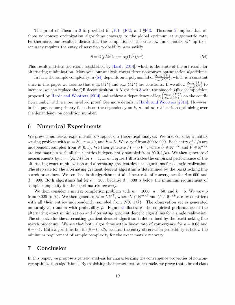
C Partition Algorithm for Matrix Computation
Algorithm 4 The observation set partition algorithm for matrix completion. It guarantees the
independence among all 2T + 1 output observation sets.
Input: W, ρ
ρ = 1− (1− ρ)1
2T+1 .
For: t = 0, ...., 2T
ρt =(mn)!ρt+1(1− ρ)mn−t−1
ρ(mn− t− 1)!(t+ 1)!End for
W0 = ∅, ..., W2T = ∅For every (i, j) ∈ W
Sample t from 0, ..., 2T with probability ρ0, ..., ρ2T Sample (w/o replacement) a set B such that |B| = t from 0, ..., 2T with equal probability
Add (i, j) to W` for all ` ∈ BEnd for
Output: Wt2Tt=0, ρ
D Initialization Procedures for Matrix Computation
Algorithm 5 The initialization procedure INTU (·) for matrix completion. It guarantees that the
initial solutions satisfy the incoherence condition throughout all iterations.
Input: M
Parameter: Incoherence parameter µ
(U , D, V )← KSVD(M)
U tmp ← argminU‖U − U‖2F subject to max
i‖Ui∗‖2 ≤ µ
√k/m
(Uout, Rout
U)← QR(U tmp)
V tmp ← argminV
‖V − V tmp‖2F subject to maxj‖Vj∗‖2 ≤ µ
√k/n
(Vout, Rout
V)← QR(V tmp)
V out = Vout
(Uout>
MVout
)>
Output: Uout
, V out
E Lemmas for Theorem 2 (Alternating Exact Minimization)
E.1 Proof of Lemma 21
Proof. For notational convenience, we omit the index t in U∗(t)
and V ∗(t), and denote them by
U∗
and V ∗ respectively. Before we proceed with the main proof, we first introduce the following
33

Algorithm 6 The initialization procedure INTV (·) for matrix completion. It guarantees that the
initial solutions satisfy the incoherence condition throughout all iterations.
Input: M
Parameter: Incoherence parameter µ
(U , D, V )← KSVD(M)
V tmp ← argminV
‖V − V ‖2F subject to maxj‖Vj∗‖2 ≤ µ
√k/n
(Vout, Rout
V)← QR(V tmp)
U tmp ← argminU‖U − U tmp‖2F subject to max
i‖Ui∗‖2 ≤ µ
√k/m
(Uout, Rout
U)← QR(U tmp)
Uout = Uout
(Uout>
MVout
)
Output: Vout
, Uout
lemma.
Lemma 18. Suppose that ρ satisfies (93). For any z ∈ Rm and w ∈ Rn such that∑
i zi = 0, and
a t ∈ 0, ..., 2T, there exists a universal constant C such that∑(i,j)∈Wt
ziwj ≤ Cm1/4n1/4ρ1/2‖z‖2‖w‖2
with probability at least 1− n−3.
The proof of Lemma 18 is provided in Keshavan et al. [2010a], and therefore omitted.
We then proceed with the proof of Lemma 21. For j = 1, ..., k, we define S(j,t), J (j,t), and K(j,t)
as
S(j,t) =1
ρ
∑i:(i,j)∈W2t+1
U(t)i∗ U
(t)>i∗ , J (j,t) =
1
ρ
∑i:(i,j)∈W2t+1
U(t)i∗ U
∗>i∗ , and K(j,t) = U
(t)>U∗.
We then consider an arbitrary W ∈ Rn×k such that ‖W‖F = 1 and w = vec(W ). Then we have
maxjσmax(S(j,t)) ≥ w>S(t)w =
∑j=1
W>j∗S(j,t)Wj∗ ≥ min
jσmin(S(j,t)). (85)
SinceW2t+1 is drawn uniformly at random, we can use mn independent Bernoulli random variables
δij ’s to describeW2t+1, i.e., δiji.i.d.∼ Bernoulli(ρ) with δij = 1 denoting (i, j) ∈ W2t+1 and 0 denoting
(i, j) /∈ W2t+1. We then consider an arbitrary z ∈ Rk with ‖z‖2 = 1, and define
Y = z>S(j,t)z =1
ρ
∑i:(i,j)∈W2t+1
(z>U
(t)i∗)2
=1
ρ
∑i
δij(z>U
(t)i∗)2.
Then we have
EY = z>U(t)U
(t)>z = 1 and EY 2 =
1
ρ
∑i
δij(z>U
(t)i∗)4 ≤ 4µ2k
mρ
∑i
(z>U
(t)i∗)2
=4µ2k
mρ,
34

where the last inequality holds, since U(t)
is incoherent with parameter 2µ. Similarly, we can show
maxi
(z>U
(t)i∗)2 ≤ 4µ2k
mρ.
Thus by Bernstein’s inequality, we obtain
P (|Y − EY | ≥ δ2k) ≤ exp
(−
3δ22k6 + 2δ2k
mρ
4µ2k
).
Since ρ and δ2k satisfy (53) and (95), then for a sufficiently large C7, we have
P (|Y − EY | ≥ δ2k) ≤1
n3,
which implies that for any z and j, we have
P(1 + δ2k ≥ z>S(j,t)z ≥ 1− δ2k
)≥ 1− n−3. (86)
Combining (86) with (85), we complete the proof.
E.2 Proof of Lemma 22
Proof. For notational convenience, we omit the index t in U∗(t)
and V ∗(t), and denote them by U∗
and V ∗ respectively. Let H(j,t) = S(j,t)K(j,t) − J (j,t). We have
H(j,t) =1
ρ
∑i:(i,j)∈W2t+1
U(t)i∗ U
(t)>i∗ U
(t)>U∗ − U i∗U
>i∗ =
1
ρ
∑i:(i,j)∈W2t+1
H(i,j,t).
We consider an arbitrary Z ∈ Rn×k such that ‖Z‖F = 1. Let z = vec(Z) and v = vec(V ). Since∑i
H(i,j,t) = U(t)>
U(t)U
(t)>U∗ − U (t)>
U∗
= 0,
then by Lemma 18, we have
z>(S(t)K(t) − J (t))v =∑j
Z>∗j(S(j,t)K(t) − J (j,t))Vj∗ ≤
1
ρ
∑p,q
√∑j
Z2pj(Vjq)
2
√∑i
[H(i,j,t)]2pq.
Meanwhile, we have∑i
[H(i,j,t)]2pq =∑i
(U(t)ip )2(U
(t)>i∗ U
(t)>U∗∗q − U
∗iq)
2 ≤ maxi
(U(t)ip )2
∑i
(U(t)>i∗ U
(t)>U∗∗q − U
∗iq)
2
= maxi
(U(t)ip )2(1− ‖U (t)>
U∗∗q‖22) ≤ max
i‖U (t)
i∗ ‖22(1− (U(t)>∗q U
∗∗q)
2)
(i)
≤ 4µ2k
m(1− U (t)>
∗q U∗∗q)(1 + U
(t)>∗q U
∗∗q)
(ii)
≤ 4µ2k
m‖U∗q − U
∗∗q‖22 ≤
4√
2µ2k
m‖U (t) − U∗‖2F,
35

where (i) comes from the incoherence of U(t)
, and (ii) comes from U(t)>∗q U
∗∗q ≤ ‖U
(t)∗q ‖2‖U
∗∗q‖2 ≤ 1.
Combining the above inequalities, by the incoherence of V and Bernstein’s inequality, we have
z>(S(t)K(t) − J (t))v ≤∑p,q
4σ1µ2k
mρ‖U (t) − U∗‖F‖Z∗p‖2 ≤ 3kσ1δ2k‖U
(t) − U∗‖F
with probability at least 1 − n−3, where the last inequality comes from the incoherence of V ,∑p ‖Z∗p‖2 ≤
√k, and a sufficiently large ρ. Since z is arbitrary, then we have
P(‖(S(t)K(t) − J (t))v‖2 ≤ 3δ2kkσ1‖U
(t) − U∗‖F)≥ 1− n−3,
which completes the proof.
E.3 Proof of Lemma 26
Proof. Recall that we have W in = V (t+0.5) and V(t+1)
= W out in Algorithm 3. Since V (t+0.5)
satisfies (5) of Lemma 5, then there exists a factorization of M∗ = U∗(t+0.5)V∗(t+0.5)>
such that
V∗(t+0.5)
is an orthonormal matrix, and satisfies
‖W in − V ∗(t+0.5)‖F ≤2
σk‖W in − V ∗(t)‖F ≤
2
σk· σk
8=
1
4. (87)
Since the Frobenius norm projection is contractive, then we have
‖W − V ∗(t+0.5)‖F ≤ ‖Win − V ∗(t+0.5)‖F ≤
1
4. (88)
Since V∗(t+0.5)
is an orthonormal matrix, by Lemma 14, we have
‖W out − V ∗(t+1)‖F ≤√
2‖V ∗(t+0.5)†‖2‖W − V∗(t+0.5)‖F
1− ‖W in − V ∗(t+0.5)‖F‖V∗(t+0.5)†‖2
≤ 2‖W − V ∗(t+0.5)‖F ≤1
2, (89)
where V∗(t+1)
= V∗(t+0.5)
O for some unitary matrix O ∈ Rk×k, and the last inequality comes from
(88). Moreover, since V∗(t+1)
is an orthonormal matrix, then we have
σmin(W ) ≥ σmin(V∗(t+1)
)− ‖W − V ∗(t+1)‖F ≥ 1− 1
2=
1
2.
where the last inequality comes from (89). Since Wout
= W (Rtmp
W)−1, then we have
‖W outi∗ ‖2 ≤ ‖W
out>ei‖2 = ‖(R
W)−1‖2‖W>ei‖2 ≤ σ−1min(W )µ
√k
n≤ 2µ
√k
n.
36
E.4 Proof of Lemma 27
Proof. Before we proceed with the main proof, we first introduce the following lemma.
Lemma 19. Suppose that ρ satisfies (93). Recall that U , Σ, and V are defined in Algorithm 2.
There exists a universal constant C such that
‖U ΣV > −M∗‖2 = C
√k
ρ√mn
with high probability.
The proof of Lemma 19 is provided in Keshavan et al. [2010a], therefore omitted.
We then proceed with the proof of Lemma 27. Since both U ΣV > and M∗ are rank k matrices,
then U ΣV −M∗ has at most rank 2k. Thus by Lemma 19, we have
‖U ΣV > −M∗‖2F ≤ 2k‖U ΣV > −M∗‖22 ≤2Ck2
ρ√mn‖M∗‖2F ≤
2Ck3σ21ρ√mn
≤σ6k(1− δ2k)
1024(1 + δ2k)σ41ξ
2(90)
with high probability, where the last inequality comes from (93) with
C7 ≥2048(1 + δ2k)
2σ61ξ2
µ2σ6k(1− δ2k)2.
Suppose that M∗ has a rank k singular value decomposition M∗ = U∗D∗V ∗>. Then we have
‖U ΣV > −M∗‖2F = ‖U∗D∗V ∗> − U ΣV >‖2F= ‖U∗D∗V ∗> − U U>U∗D∗V ∗> + U U>U∗D∗V ∗> − U ΣV >‖2F= ‖(Im − U U>)U∗D∗V ∗> + U(U>U∗D∗V ∗> − ΣV >)‖2F≥ ‖(Im − U UT )U∗D∗V ∗>‖2F.
Let U⊥ ∈ Rm×(m−k) denote the orthogonal complement to U . Then we have
‖(Im − U UT )U∗D∗V ∗>‖2F = ‖(U⊥U>⊥ )U∗D∗V ∗>‖22 = ‖U>⊥ U∗D∗‖2F ≥σ2k2‖U>⊥ U∗‖2F.
Thus Lemma 2 guarantees that for O = argminO>O=Ik‖U − U∗O‖F, we have
‖U − U∗O‖F ≤√
2‖U>⊥ U∗‖F ≤2
σk‖U ΣV > −M∗‖F.
We define U∗tmp = U∗O. Then combining the above inequality with (90), we have
‖U − U∗tmp‖F ≤2
σk‖U ΣV > −M∗‖F ≤
σ2k(1− δ2k)16(1 + δ2k)σ
21ξ.
Since the Frobenius norm projection is contractive, then we have
‖U tmp − U∗tmp‖F ≤ ‖U − U∗tmp‖F ≤σ2k(1− δ2k)
16(1 + δ2k)σ21ξ≤ 1
16, (91)
37

where the last inequality comes from the definition of ξ and σ1 ≥ σk. Since U∗tmp is an orthonormal
matrix, by Lemma 14, we have
‖Uout − U∗(0)‖F ≤√
2U∗tmp†‖U tmp − U∗tmp‖F1− ‖U tmp − U∗tmp‖F‖U∗tmp†‖2
≤ 2‖U tmp − U∗tmp‖F ≤σ2k(1− δ2k)
8(1 + δ2k)σ21ξ≤ 1
8, (92)
where U∗(0)
= U∗tmpOtmp for some unitary matrix Otmp ∈ Rk×k such that OtmpOtmp> = Ik, and
the last inequality comes from (91). Moreover, since U∗(0)
is an orthonormal matrix, then we have
σmin(U tmp) ≥ σmin(U∗(0)
)− ‖U tmp − V ∗(t+1)‖F ≥ 1− 1
8=
7
8,
where the last inequality comes from (91). Since Uout
= U tmp(RoutU
)−1, then we have
‖Uouti∗ ‖2 ≤ ‖U
out>ei‖2 = ‖(Rout
U)−1‖2‖U>ei‖2 ≤ σ−1min(U tmp)µ
√k
m≤ 8µ
7
√k
m.
Moreover, we define V ∗(0) = M∗>U∗(0)
. Then we have U∗(0)
V ∗(0)> = U∗(0)
U∗(0)>
M∗ = M∗, where
the last inequality comes from the fact that U∗(0)
U∗(0)>
is exactly the projection matrix for the
column space of M∗.
E.5 Proof of Corollary 5
Proof. Since E(t)U implies that E(t)U,1,..., and E(t)U,4 hold with probability at least 1 − 4n−3, then com-
bining Lemmas 24 and 25, we obtain
‖V (t+0.5) − V ∗(t)‖F ≤σk2ξ‖U (t) − U∗(t)‖F
(i)
≤ σk2ξσ1
· σk(1− δ2k)4(1 + δ2k)σ1
=σ2k(1− δ2k)
8(1 + δ2k)σ21ξ
2
(ii)
≤ σk8
with probability at least 1 − 4n−3, where (i) comes from the definition of E(t)U , and (ii) comes
from the definition of ξ and σ1 ≥ σk. Therefore Lemma 26 implies that V(t+1)
is incoherent with
parameter 2µ, and
‖V (t+1) − V ∗(t+1)‖F ≤4
σk‖V (t+0.5) − V ∗(t)‖F ≤
2
ξ‖U (t) − U∗(t)‖F ≤
σk(1− δ2k)4(1 + δ2k)σ1
with probability at least 1 − 4n−3, where the last inequality comes from the definition of ξ and
E(t)U .
F Proof of Theorem 2
We present the technical proof for matrix completion. Before we proceed with the main proof, we
first introduce the following lemma.
38

Lemma 20. [Hardt and Wootters [2014]] Suppose that the entry observation probability ρ of Wsatisfies (53). Then the output sets Wt2Tt=0, of Algorithm 4 are equivalent to 2T + 1 observation
sets, which are independently generated with the entry observation probability
ρ ≥ C7µ2k3 log n
m(93)
for some constant C7.
See Hardt and Wootters [2014] for the proof of Lemma 20. Lemma 20 ensures the independence
among all observation sets generated by Algorithm 4. To make the convergence analysis for matrix
completion comparable to that for matrix sensing, we rescale both the objective function FW and
step size η by the entry observation probability ρ of each individual set, which is also obtained by
Algorithm 4. In particular, we define
FW(U, V ) =1
2ρ‖PW(UV >)− PW(M∗)‖2F and η = ρη. (94)
For notational simplicity, we assume that at the t-th iteration, there exists a matrix factorization
of M∗ as
M∗ = U∗(t)
V ∗(t)>,
where U∗(t) ∈ Rm×k is an orthonormal matrix. Then we define several nk × nk matrices
S(t) =
S(t)11 · · · S
(t)1k
.... . .
...
S(t)k1 · · · S
(t)kk
with S(t)pq =
1
ρ
∑i:(i,1)∈W2t+1
U(t)ip U
(t)iq · · · 0
.... . .
...
0 · · · 1
ρ
∑i:(i,n)∈W2t+1
U(t)ip U
(t)iq
,
G(t) =
G
(t)11 · · · G
(t)1k
.... . .
...
G(t)k1 · · · G
(t)kk
with G(t)pq =
1
ρ
∑i:(i,1)∈W2t+1
U∗(t)ip U
∗(t)iq · · · 0
.... . .
...
0 · · · 1
ρ
∑i:(i,n)∈W2t+1
U∗(t)ip U
∗(t)iq
,
J (t) =
J(t)11 · · · J
(t)1k
.... . .
...
J(t)k1 · · · J
(t)kk
with J (t)pq =
1
ρ
∑i:(i,1)∈W2t+1
U(t)ip U
∗(t)iq · · · 0
.... . .
...
0 · · · 1
ρ
∑i:(i,n)∈W2t+1
U(t)ip U
∗(t)iq
,
K(t) =
K
(t)11 · · · K
(t)1k
.... . .
...
K(t)k1 · · · K
(t)kk
with K(t)pq = U
(t)>∗p U
∗(t)∗q In,
39

where 1 ≤ p, q ≤ k. Note that S(t) and G(t) are the partial Hessian matrices ∇2V FW2t+1(U
(t), V )
and ∇2V FW2t+1(U
∗(t), V ) with respect to a vectorized V , i.e., vec(V ).
F.1 Proof of Theorem 2 (Alternating Exact Minimization)
Proof. Throughout the proof for alternating exact minimization, we define a constant ξ ∈ (2,∞)
to simplify the notation. We define the approximation error of the inexact first order oracle as
E(V (t+0.5), V (t+0.5), U(t)
) = ‖∇V FW2t+1(U∗(t)
, V (t+0.5))−∇V FW2t+1(U(t), V (t+0.5))‖F.
To simplify our later analysis, we first introduce the following event.
E(t)U =
‖U (t) − U∗(t)‖F ≤
(1− δ2k)σk4ξ(1 + δ2k)σ1
and maxi‖U (t)
i∗ ‖2 ≤ 2µ
√k
m
.
We then present two important consequences of E(t)U .
Lemma 21. Suppose that E(t)U holds, and ρ satisfies (93). Then we have
P(1 + δ2k ≥ σmax(S(t)) ≥ σmin(S(t)) ≥ 1− δ2k
)≥ 1− n−3,
where δ2k is some constant satisfying
δ2k ≤σ6k
192ξ2kσ61. (95)
The proof of Lemma 21 is provided in Appendix E.1. Lemma 21 is also applicable to G(t), since
G(t) shares the same structure with S(t), and U∗(t)
is incoherent with parameter µ.
Lemma 22. Suppose that E(t)U holds, and ρ satisfies (93). Then for an incoherent V with parameter
3σ1µ, we have
P(‖(S(t)K(t) − J (t)) · vec(V )‖2 ≤ 3kσ1δ2k‖U
(t) − U∗(t)‖F)≥ 1− n−3,
where δ2k is defined in (95).
The proof of Lemma 22 is provided in Appendix E.2. Note that Lemma 22 is also applicable to
‖(G(t)K(t)− J (t)) · vec(V )‖2, since G(t) shares the same structure with S(t), and U∗(t)
is incoherent
with parameter µ.
We then introduce another two events:
E(t)U,1 = 1 + δ2k ≥ σmax(S(t)) ≥ σmin(S(t)) ≥ 1− δ2k,
E(t)U,2 = 1 + δ2k ≥ σmax(G(t)) ≥ σmin(G(t)) ≥ 1− δ2k,
where δ2k is defined in E(t)U . By Lemmas 21, we can verify that E(t)U implies E(t)U,1 and E(t)U,2 with
probability at least 1− 2n−3. The next lemma shows that E(t)U,1 and E(t)U,2 imply the strong convexity
and smoothness of FW2t+1(U, V ) in V at U = U(t)
and U∗(t)
.
40

Lemma 23. Suppose that E(t)U,1 and E(t)U,2 hold. Then for any V, V ′ ∈ Rn×k, we have
1 + δ2k2‖V ′ − V ‖2F ≥ FW2t+1(U
(t), V ′)−FW2t+1(U
(t), V )
− 〈∇V FW2t+1(U(t), V ), V ′ − V 〉 ≥ 1− δ2k
2‖V ′ − V ‖2F,
1 + δ2k2‖V ′ − V ‖2F ≥ FW2t+1(U
∗(t), V ′)−FW2t+1(U
∗(t), V )
− 〈∇V FW2t+1(U∗(t)
, V ), V ′ − V 〉 ≥ 1− δ2k2‖V ′ − V ‖2F.
Since S(t) andG(t) are essentially the partial Hessian matrices∇2V FW2t+1(U
(t), V ) and∇2
V FW2t+1(U∗(t)
, V ),
the proof of 23 directly follows Appendix A.1, and is therefore omitted.
We then introduce another two events:
E(t)U,3 = ‖(S(t)K(t) − J (t)) · vec(V ∗(t))‖2 ≤ 3kσ1δ2k‖U(t) − U∗(t)‖F,
E(t)U,4 = ‖(G(t)K(t) − J (t)) · vec(V ∗(t))‖2 ≤ 3kσ1δ2k‖U(t) − U∗(t)‖F,
where δ2k is defined in E(t)U . We can verify that E(t)U implies E(t)U,3 and E(t)U,4 with probability at least
1 − 2n−3 by showing the incoherence of V ∗(t). More specifically, let V ∗(t) = V∗(t)
R∗(t)V denote the
QR decomposition of V ∗(t). We have
‖V ∗(t)j∗ ‖2 = ‖R∗(t)>V V ∗(t)>ej‖2 ≤ ‖R∗(t)V ‖2‖V∗(t)>ej‖2 ≤ σ1‖V ∗(t)j∗ ‖2 ≤ σ1µ
√k
n. (96)
Then Lemma 22 are applicable to E(t)U,3 and E(t)U,4.We then introduce the following key lemmas, which will be used in the main proof.
Lemma 24. Suppose that E(t)U , E(t)U,1,..., and E(t)U,4 hold. We then have
E(V (t+0.5), V (t+0.5), U(t)
) ≤ (1− δ2k)σk2ξ
‖U (t) − U∗(t)‖F.
Lemma 24 shows that the approximation error of the inexact first order oracle for updating V
diminishes with the estimation error of U (t), when U (t) is sufficiently close to U∗(t). It is analogous
to Lemma 3 in the analysis of matrix sensing, and its proof directly follows A.2, and is therefore
omitted.
Lemma 25. Suppose that E(t)U , E(t)U,1,..., and E(t)U,4 hold. We then have
‖V (t+0.5) − V ∗(t)‖F ≤1
1− δ2kE(V (t+0.5), V (t), U
(t)).
Lemma 25 illustrates that the estimation error of V (t+0.5) diminishes with the approximation
error of the inexact first order oracle. It is analogous to Lemma 4 in the analysis of matrix sensing,
and its proof directly follows Appendix A.3, and is therefore omitted.
41

Lemma 26. Suppose that V (t+0.5) satisfies
‖V (t+0.5) − V ∗(t)‖F ≤σk8. (97)
Then there exists a factorization of M∗ = U∗(t+1)V∗(t+1)>
such that V∗(t+1) ∈ Rn×k is an orthonor-
mal matrix, and satisfies
maxj‖V (t+1)
j∗ ‖2 ≤ 2µ
√2k
nand ‖V (t+1) − V ∗(t+1)‖F ≤
4
σk‖V (t+0.5) − V ∗‖F.
The proof of Lemma 26 is provided in Appendix E.3. Lemma 26 ensures that the incoherence
factorization enforces V(t+1)
to be incoherent with parameter 2µ.
Lemma 27. Suppose that ρ satisfies (93). Then E(0)U holds with high probability.
The proof of Lemma 27 is provided in §E.4. Lemma 27 shows that the initial solution U(0)
is incoherent with parameter 2µ, while achieving a sufficiently small estimation error with high
probability. It is analogous to Lemma 6 for matrix sensing.
Combining Lemmas 24, 25, and 26, we obtain the next corollary for a complete iteration of
updating V .
Corollary 5. Suppose that E(t)U holds. Then
E(t)V =
‖V (t+1) − V ∗(t+1)‖F ≤
(1− δ2k)σk4ξ(1 + δ2k)σ1
and maxj‖V (t+1)
j∗ ‖2 ≤ 2µ
√k
m
holds with probability at least 1− 4n−3. Moreover, we have
‖V (t+1) − V ∗‖F ≤2
ξ‖U (t) − U∗(t)‖F and ‖V (t+0.5) − V ∗(t)‖F ≤
σk2ξ‖U (t) − U∗(t)‖F
with probability at least 1− 4n−3.
The proof of Corollary 5 is provided in Appendix E.5. Since the alternating exact minimization
algorithm updates U and V in a symmetric manner, we can establish similar results for a complete
iteration of updating U in the next corollary.
Corollary 6. Suppose E(t)V holds. Then E(t+1)U holds with probability at least 1− 4n−3. Moreover,
we have
‖U (t+1) − U∗(t+1)‖F ≤2
ξ‖V (t+1) − V ∗(t+1)‖F and ‖U (t+0.5) − U∗(t+1)‖F ≤
σk2ξ‖V (t+1) − V ∗(t+1)‖F
with probability at least 1− 4n−3.
The proof of Lemma 6 directly follows Appendix E.5, and is therefore omitted.
42

We proceed with the proof of Theorem 2 conditioning on E(0)U . Similar to Appendix 1, we can
recursively apply Corollaries 5 and 6, and show that E(t)U Tt=1 and E(t)V Tt=0 simultaneously hold
with probability at least 1− 8Tn−3. Then conditioning on all E(t)U Tt=0 and E(t)V Tt=0, we have
‖V (T ) − V ∗(T )‖F ≤2
ξ‖U (T−1) − U∗(T−1)‖F ≤
(2
ξ
)2
‖V (T−1) − V ∗(T−1)‖F
≤(
2
ξ
)2T−1‖U (0) − U∗(0)‖F ≤
(2
ξ
)2T (1− δ2k)σk8(1 + δ2k)σ1
, (98)
where the last inequality comes from the definition of E(0)U . Thus we only need
T =
⌈1
2log−1
(ξ
2
)log
((1− δ2k)σk4(1 + δ2k)σ1
· 1
ε
)⌉iterations such that
‖V (T ) − V ∗(T )‖F ≤(
2
ξ
)2T (1− δ2k)σk8(1 + δ2k)σ1
≤ ε
2. (99)
Meanwhile, by (99) and Corollary 6, we have
‖U (T−0.5) − U∗(T )‖F ≤σk2ξ‖V (T ) − V ∗(T )‖F ≤
(2
ξ
)2T (1− δ2k)σ2k16ξ(1 + δ2k)σ1
,
where the last inequality comes from (98). Thus we only need
T =
⌈1
2log−1
(ξ
2
)log
((1− δ2k)σ2k8ξ(1 + δ2k)
· 1
ε
)⌉iterations such that
‖U (T−0.5) − U∗(T )‖F ≤(
2
ξ
)2T (1− δ2k)σ2k16ξ(1 + δ2k)σ1
≤ ε
2σ1. (100)
We then combine (99) and (100) by following similar lines to §4.2, and show
‖M (T ) −M∗‖F ≤ ε. (101)
The above analysis only depends on E(0)U . Because Lemma 27 guarantees that E(0)U holds with high
probability, given T n3, (101) also holds with high probability.
F.2 Proof of Theorem 2 (Alternating Gradient Descent)
Proof. Throughout the proof for alternating gradient descent, we define a sufficiently large constant
ξ. Moreover, we assume that at the t-th iteration, there exists a matrix factorization of M∗ as
M∗ = U∗(t)
V ∗(t)>,
43

where U∗(t) ∈ Rm×k is an orthonormal matrix. We define the approximation error of the inexact
first order oracle as
E(V (t+0.5), V (t), U(t)
) ≤ ‖FW2t+1(U(t), V (t))−∇V FW2t+1(U
∗(t), V (t))‖F
To simplify our later analysis, we introduce the following event.
E(t)U =
maxi‖U (t)
i∗ ‖2 ≤ 2µ
√k
n, ‖U (t) − U∗(t)‖F ≤
σ2k4ξσ21
maxi‖V (t)
j∗ ‖2 ≤ 2σ1µ
√k
n, and ‖V (t) − V ∗(t)‖F ≤
σ2k2ξσ1
.
As has been shown in §F.1, E(t)U implies the following four events with probability at least 1−4n−3,
E(t)U,1 =
1 + δ2k ≥ σmax(S(t)) ≥ σmin(S(t)) ≥ 1− δ2k,
E(t)U,2 =
1 + δ2k ≥ σmax(G(t)) ≥ σmin(G(t)) ≥ 1− δ2k,
E(t)U,3 =‖(S(t)K(t) − J (t)) · vec(V ∗(t))‖2 ≤ 3kσ1δ2k‖U
(t) − U∗(t)‖F,
E(t)U,4 =‖(G(t)K(t) − J (t)) · vec(V ∗(t))‖2 ≤ 3kσ1δ2k‖U
(t) − U∗(t)‖F,
where δ2k is defined in (95). In §F.1, we also show that E(t)U,1 and E(t)U,2 imply the strong convexity
and smoothness of FW2t+1(U, V ) at U = U(t)
and U∗(t)
.
Moreover, we introduce the following two events,
E(t)U,5 =‖(S(t)K(t) − J (t)) · vec(V (t) − V ∗(t))‖2 ≤ 3kσ1δ2k‖U
(t) − U∗(t)‖F,
E(t)U,6 =‖(G(t)K(t) − J (t)) · vec(V (t) − V ∗(t))‖2 ≤ 3kσ1δ2k‖U
(t) − U∗(t)‖F,
where δ2k is defined in (95). We can verify that E(t)U implies E(t)U,5 and E(t)U,6 with probability at least
1− 2n−3 by showing the incoherence of V (t) − V ∗(t). More specifically, we have
maxj‖V (t)
j∗ − V∗(t)j∗ ‖2 ≤ max
i‖V (t)
j∗ ‖2 + maxj‖V ∗(t)j∗ ‖2 ≤ 3σ1µ
√k
n,
where the last inequality follows the definition of E(t)U and the incoherence of V ∗(t) as shown in (96).
Then Lemma 22 are applicable to E(t)U,5 and E(t)U,6We then introduce the following key lemmas, which will be used in the main proof.
Lemma 28. Suppose that E(t)U , E(t)U,1, ..., and E(t)U,6 hold. Then we have
E(V (t+0.5), V (t), U(t)
) ≤ (1 + δ2k)σkξ
‖U (t) − U∗‖F.
Lemma 28 shows that the approximation error of the inexact first order oracle for updating V
diminishes with the estimation error of U (t), when U (t) is sufficiently close to U∗(t). It is analogous
to Lemma 7 in the analysis of matrix sensing, and its proof directly follows B.1, and is therefore
omitted.
44

Lemma 29. Suppose that E(t)U , E(t)U,1, ..., and E(t)U,6 hold. Meanwhile, the rescaled step size parameter
η satisfies
η =1
1 + δ2k.
Then we have
‖V (t+0.5) − V ∗(t)‖F ≤√δ2k‖V (t) − V ∗(t)‖F +
2
1 + δ2kE(V (t+0.5), V (t), U
(t)).
Lemma 29 illustrates that the estimation error of V (t+0.5) diminishes with the approximation
error of the inexact first order oracle. It is analogous to Lemma 8 in the analysis of matrix sensing.
Its proof directly follows Appendix B.2, and is therefore omitted.
Lemma 30. Suppose that V (t+0.5) satisfies
‖V (t+0.5) − V ∗(t)‖F ≤σk8.
We then have
maxj‖V (t+1)
j∗ ‖2 ≤ 2µ
√2k
nand max
i‖U (t+1)
i∗ ‖2 ≤ 2σ1µ
√2k
m
Moreover, there exists a factorization of M∗ = U∗(t+1)V∗(t+1)>
such that V∗(t+1)
is an orthonormal
matrix, and
‖V (t+1) − V ∗(t)‖F ≤4
σk‖V (t+0.5) − V ∗(t)‖F,
‖U (t) − U∗(t+1)‖F ≤5σ1σk‖V (t+0.5) − V ∗(t)‖F + σ1‖U
(t) − U∗(t)‖F.
The proof of Lemma 26 is provided in Appendix G.1. Lemma 30 guarantees that the incoherence
factorization enforces V(t+1)
and U (t) to be incoherent with parameters 2µ and 2σ1µ respectively.
The next lemma characterizes the estimation error of the initial solutions.
Lemma 31. Suppose that ρ satisfies (93). Then E(0)U holds with high probability.
The proof of Lemma 31 is provided in Appendix G.2. Lemma 31 ensures that the initial solutions
U (0), and V (0) are incoherent with parameters 2µ and 2σ1µ respectively, while achieving sufficiently
small estimation errors with high probability. It is analogous to Lemma 10 in the analysis of matrix
sensing.
Combining Lemmas 28, 29, and 26, we obtain the following corollary for a complete iteration
of updating V .
Corollary 7. Suppose that E(t)U holds. Then
E(t)V =
maxj‖V (t)
j∗ ‖2 ≤ 2µ
√k
m, ‖V (t) − V ∗(t)‖F ≤
σ2k4ξσ21
,
maxi‖U (t)
i∗ ‖2 ≤ 2σ1µ
√k
m, and ‖U (t) − U∗(t+1)‖F ≤
σ2k2ξσ1
45

holds with probability at least 1− 6n−3. Moreover, we have
‖V (t+0.5) − V ∗(t)‖F ≤√δ2k‖V (t) − V ∗(t)‖F +
2σkξ‖U (t) − U∗(t)‖F, (102)
‖V (t+1) − V ∗(t)‖F ≤4√δ2kσk‖V (t) − V ∗(t)‖F +
8
ξ‖U (t) − U∗(t)‖F, (103)
‖U (t) − U∗(t+1)‖F ≤5σ1√δ2k
σk‖V (t) − V ∗(t)‖F +
(10
ξ+ 1
)σ1‖U
(t) − U∗(t)‖F, (104)
with probability at least 1− 6n−3.
The proof of Corollary 7 is provided in Appendix G.3. Since the algorithm updates U and V
in a symmetric manner, we can establish similar results for a complete iteration of updating U in
the next corollary.
Corollary 8. Suppose E(t)V holds. Then E(t+1)U holds with probability at least 1− 6n−3. Moreover,
we have
‖U (t+0.5) − U∗(t+1)‖F ≤√δ2k‖U (t) − U∗(t+1)‖F +
2σkξ‖V (t+1) − V ∗(t+1)‖F, (105)
‖U (t+1) − U∗(t+1)‖F ≤4√δ2kσk‖U (t) − U∗(t+1)‖F +
8
ξ‖V (t+1) − V ∗(t+1)‖F, (106)
‖V (t+1) − V ∗(t+1)‖F ≤5σ1√δ2k
σk‖U (t) − U∗(t+1)‖F +
(10σ1ξ
+ 1
)‖V (t+1) − V ∗(t+1)‖F, (107)
with probability at least 1− 6n−3.
The proof of Corollary 8 directly follows Appendix G.3, and is therefore omitted.
We then proceed with the proof of Theorem 2 conditioning on E(0)U . Similar to Appendix 1, we
can recursively apply Corollaries 7 and 8, and show that E(t)U Tt=1 and E(t)V Tt=0 simultaneously
hold with probability at least 1− 12Tn−3. For simplicity, we define
φV (t+1) = ‖V (t+1) − V ∗(t+1)‖F, φV (t+0.5) = ‖V (t+0.5) − V ∗(t)‖F, φV
(t+1) = σ1‖V(t+1) − V ∗(t+1)‖F,
φU(t+1) = ‖U (t+1) − U∗(t+2)‖F, φU(t+0.5) = ‖U (t+0.5) − U∗(t+1)‖F, φU
(t+1) = σ1‖U(t+1) − U∗(t+1)‖F.
We then follow similar lines to §4.3 and §F.1, and show that ‖M (T )−M‖F ≤ ε with high probability.
F.3 Proof of Theorem 2 (Gradient Descent)
Proof. The convergence analysis of the gradient descent algorithm is similar to alternating gradient
descent. The only difference is, for updating U , gradient descent uses V = V(t)
instead of V =
V(t+1)
to calculate the gradient at U = U (t). Then everything else directly follows Appendix F.2,
and is therefore omitted.
46

G Lemmas for Theorem 2 (Alternating Gradient Descent)
G.1 Proof of Lemma 30
Proof. Recall that we have W in = V (t+0.5) and V(t+1)
= W out in Algorithm 3. By Lemma 26, we
can show
‖W out − V ∗(t+1)‖F ≤4
σk‖V (t+0.5) − V ∗(t)‖F. (108)
By Lemma 17, we have
‖R(t+0.5)
V− V ∗(t+1)>
V ∗(t)‖F = ‖V (t+1)>V (t+0.5) − V ∗(t+1)>
V ∗(t)‖F
≤ ‖V (t+1)‖2‖V (t+0.5) − V ∗(t)‖F + ‖V ∗(t)‖2‖V(t+1) − V ∗(t+1)‖F
≤ ‖V (t+0.5) − V ∗(t)‖F +4σ1σk‖V (t+0.5) − V ∗(t)‖F, (109)
where the last inequality comes from (108), ‖V (t+1)‖2 = 1, and ‖V ∗(t)‖2 = σ1. Moreover, we define
U∗(t+1) = U∗(t)
(V∗(t+1)>
V ∗(t))>. Then we can verify
U∗(t+1)V∗(t+1)
= U∗(t)
V ∗(t)>V∗(t+1)
V∗(t+1)>
= M∗,
where the last equality holds since V∗(t+1)
V∗(t+1)
is exactly the projection matrix for the row space
of M∗. Thus we further have
‖U (t) − U∗(t+1)‖F = ‖U (t)(V
(t+1)>V (t+0.5))> − U∗(t)(V ∗(t+1)>
V ∗(t))>‖F
≤ ‖U (t)‖2‖R(t+0.5)
V− V ∗(t+1)>
V ∗(t)‖F + ‖V ∗(t+1)>V ∗(t)‖2‖U
(t) − U∗(t)‖F
≤ 5σ1σk‖V (t+0.5) − V ∗(t)‖F + σ1‖U
(t) − U∗(t)‖F,
where the last inequality comes from (109), ‖U (t)‖2 = 1, ‖V ∗(t+1)>V ∗(t)‖2 = σ1, and σ1 ≥ σk.
G.2 Proof of Lemma 31
Proof. Following similar lines to Appendix E.4, we can obtain
maxi‖U (0)
i∗ ‖2 ≤8µ
7
√k
m, ‖U (0) − U∗(0)‖F ≤
σ2k8ξσ21
, (110)
maxj‖V (0)
j∗ ‖2 ≤8µ
7
√k
n, ‖V (0) − V ∗(0)‖F ≤
σ2k8ξσ21
. (111)
Then by Lemma 17, we have
‖U (0)>M − U∗(0)>M∗‖F ≤ ‖U
(0)‖2‖M −M∗‖F + ‖M∗‖2‖U(0) − U∗(0)‖F
≤ σ3132ξσ2k
+σ2k
8ξσ1≤
5σ2k32ξσ1
. (112)
47
By Lemma 17 again, we have
‖V (0)>M>U
(0) − V ∗(0)>M∗>U∗(0)‖F
≤ ‖V (0)‖2‖M>U(0) −M∗>U∗(0)‖F + ‖U∗(0)>M∗‖2‖V
(0) − V ∗(0)‖F
≤5σ2k
32ξσ1+
σ2k8ξσ1
≤9σ2k
32ξσ1, (113)
where the last inequality comes from (111) and (112), and ‖M∗‖2 = σ1. By Lemma 17 again, we
have
‖V (0) − V ∗(0)‖F ≤ ‖V(0)V
(0)>M>U
(0) − V ∗(0)V ∗(0)>M∗>U∗(0)‖F
≤ ‖V (0)‖2‖V(0)>
M>U(0) − V ∗(0)>M∗>U∗(0)‖F + ‖U∗(0)>M∗V ∗(0)‖2‖V
(0) − V ∗(0)‖F
≤9σ2k
32ξσ1+
σ2k8ξσ1
≤13σ2k32ξσ1
, (114)
where the last two inequalities come from (111), (114), and ‖U∗(0)>M∗V ∗(0)‖2 ≤ σ1, the definition
of ξ, and σ1 ≥ σk. Moreover, by the incoherence of V (0), we have
‖V (0)j∗ ‖2 ≤ ‖V
(0)>ej‖2 = ‖V (0)>M>U
(0)‖2‖V(0)>
ei‖2
≤(‖V ∗(0)V ∗(0)>M∗>U∗(0)‖2 + ‖V (0)>
M>U(0) − V ∗(0)V ∗(0)>M∗>U∗(0)‖F
) 6µ
5
√k
m
≤(
1 +9σ2k
32ξσ21
)6σ1µ
5
√k
m≤ 41σ1µ
28
√k
m,
where the last two inequalities come from (111), (114), the definition of ξ, and σ1 ≥ σk
G.3 Proof of Corollary 7
Proof. Since E(t)U implies that E(t)U,1,...,E(t)U,6 hold with probability 1− 6n−3, then combining Lemmas
28 and 29, we obtain
‖V (t+0.5) − V ∗(t)‖F ≤√δ2k‖V (t) − V ∗(t)‖F +
2
1 + δ2kE(V (t+0.5), V (t), U
(t))
≤√δ2k‖V (t) − V ∗(t)‖F +
2σkξ‖U (t) − U∗(t)‖F
≤σ3k
12ξσ31·σ2k
2ξσ1+
2σ2kξ
σk4ξσ21
=σ5k
24ξ2σ41+
σ3k2ξ2σ21
≤ σk8
with probability 1 − 6n−3, where the last inequality comes from the definition of ξ and σ1 ≥ σk.
Thus by Lemma 30, we have
‖V (t+1) − V ∗(t+1)‖F ≤4√δ2kσk‖V (t) − V ∗(t)‖F +
8
ξ‖U (t) − U∗(t)‖F
≤ 4
σk
(σ5k
24ξ2σ41+
σ3k2ξ2σ21
)=
σ4k6ξ2σ41
+2σ2kξ2σ21
≤σ2k
4ξσ21,
48

with probability 1 − 6n−3, where the last inequality comes from the definition of ξ and σ1 ≥ σk.
Moreover, by Lemma 30 again, we have
‖U (t) − U∗(t+1)‖F ≤5σ1√δ2k
σk‖V (t) − V ∗(t)‖F +
(10
ξ+ 1
)σ1‖U
(t) − U∗(t)‖F
≤ 5σ1σk·
σ3k12ξσ31
·σ2k
2ξσ1+
(10
ξ+ 1
)σ1
σ2k4ξσ21
=5σ4k
24ξ2σ31+
σ2k3ξσ1
≤σ2k
2ξσ1
with probability 1−6n−3, where the last inequality comes from the definition of ξ and σ1 ≥ σk.
References
Alekh Agarwal, Sahand Negahban, and Martin J Wainwright. Noisy matrix decomposition via
convex relaxation: Optimal rates in high dimensions. The Annals of Statistics, 40(2):1171–1197,
2012.
Sanjeev Arora, Rong Ge, Tengyu Ma, and Ankur Moitra. Simple, efficient, and neural algorithms
for sparse coding. arXiv preprint arXiv:1503.00778, 2015.
Michel Baes. Estimate sequence methods: extensions and approximations. Institute for Operations
Research, ETH, Zurich, Switzerland, 2009.
Sivaraman Balakrishnan, Martin J Wainwright, and Bin Yu. Statistical guarantees for the EM
algorithm: From population to sample-based analysis. arXiv preprint arXiv:1408.2156, 2014.
Srinadh Bhojanapalli, Anastasios Kyrillidis, and Sujay Sanghavi. Dropping convexity for faster
semi-definite optimization. arXiv preprint arXiv:1509.03917, 2015.
Jian-Feng Cai, Emmanuel J Candes, and Zuowei Shen. A singular value thresholding algorithm for
matrix completion. SIAM Journal on Optimization, 20(4):1956–1982, 2010.
T Tony Cai and Anru Zhang. ROP: Matrix recovery via rank-one projections. The Annals of
Statistics, 43(1):102–138, 2015.
Emmanuel Candes, Xiaodong Li, and Mahdi Soltanolkotabi. Phase retrieval via wirtinger flow:
Theory and algorithms. arXiv preprint arXiv:1407.1065, 2014.
Emmanuel J Candes and Yaniv Plan. Matrix completion with noise. Proceedings of the IEEE, 98
(6):925–936, 2010.
Emmanuel J Candes and Benjamin Recht. Exact matrix completion via convex optimization.
Foundations of Computational Mathematics, 9(6):717–772, 2009.
Emmanuel J Candes and Terence Tao. The power of convex relaxation: Near-optimal matrix
completion. IEEE Transactions on Information Theory, 56(5):2053–2080, 2010.
Venkat Chandrasekaran, Sujay Sanghavi, Pablo A Parrilo, and Alan S Willsky. Rank-sparsity
incoherence for matrix decomposition. SIAM Journal on Optimization, 21(2):572–596, 2011.
49

Jianhui Chen, Jiayu Zhou, and Jieping Ye. Integrating low-rank and group-sparse structures for
robust multi-task learning. In Proceedings of the 17th ACM SIGKDD international conference
on Knowledge discovery and data mining, pages 42–50. ACM, 2011.
Yudong Chen. Incoherence-optimal matrix completion. arXiv preprint arXiv:1310.0154, 2013.
Yudong Chen and Martin J. Wainwright. Fast low-rank estimation by projected gradient descent:
General statistical and algorithmic guarantees. arXiv preprint arXiv:1509.03025, 2015.
Yudong Chen, Srinadh Bhojanapalli, Sujay Sanghavi, and Rachel Ward. Coherent matrix comple-
tion. arXiv preprint arXiv:1306.2979, 2013a.
Yudong Chen, Ali Jalali, Sujay Sanghavi, and Constantine Caramanis. Low-rank matrix recovery
from errors and erasures. IEEE Transactions on Information Theory, 59(7):4324–4337, 2013b.
Alexandre d’Aspremont. Smooth optimization with approximate gradient. SIAM Journal on Op-
timization, 19(3):1171–1183, 2008.
Olivier Devolder, Francois Glineur, and Yurii Nesterov. First-order methods of smooth convex
optimization with inexact oracle. Mathematical Programming, 146(1-2):37–75, 2014.
Michael P Friedlander and Mark Schmidt. Hybrid deterministic-stochastic methods for data fitting.
SIAM Journal on Scientific Computing, 34(3):A1380–A1405, 2012.
Rainer Gemulla, Erik Nijkamp, Peter J Haas, and Yannis Sismanis. Large-scale matrix factorization
with distributed stochastic gradient descent. In ACM SIGKDD International Conference on
Knowledge Discovery and Data Mining, pages 69–77, 2011.
David Gross. Recovering low-rank matrices from few coefficients in any basis. IEEE Transactions
on Information Theory, 57(3):1548–1566, 2011.
Osman Guler. New proximal point algorithms for convex minimization. SIAM Journal on Opti-
mization, 2(4):649–664, 1992.
Moritz Hardt. Understanding alternating minimization for matrix completion. In Symposium on
Foundations of Computer Science, pages 651–660, 2014.
Moritz Hardt and Mary Wootters. Fast matrix completion without the condition number. arXiv
preprint arXiv:1407.4070, 2014.
Moritz Hardt, Raghu Meka, Prasad Raghavendra, and Benjamin Weitz. Computational limits for
matrix completion. arXiv preprint arXiv:1402.2331, 2014.
Trevor Hastie, Rahul Mazumder, Jason Lee, and Reza Zadeh. Matrix completion and low-rank svd
via fast alternating least squares. arXiv preprint arXiv:1410.2596, 2014.
Cho-Jui Hsieh and Peder Olsen. Nuclear norm minimization via active subspace selection. In
International Conference on Machine Learning, pages 575–583, 2014.
50

Daniel Hsu, Sham M Kakade, and Tong Zhang. Robust matrix decomposition with sparse corrup-
tions. IEEE Transactions on Information Theory, 57(11):7221–7234, 2011.
Prateek Jain and Praneeth Netrapalli. Fast exact matrix completion with finite samples. arXiv
preprint arXiv:1411.1087, 2014.
Prateek Jain, Raghu Meka, and Inderjit S Dhillon. Guaranteed rank minimization via singular
value projection. In Advances in Neural Information Processing Systems, pages 937–945, 2010.
Prateek Jain, Praneeth Netrapalli, and Sujay Sanghavi. Low-rank matrix completion using alter-
nating minimization. In Symposium on Theory of Computing, pages 665–674, 2013.
Raghunandan H Keshavan, Andrea Montanari, and Sewoong Oh. Matrix completion from a few
entries. IEEE Transactions on Information Theory, 56(6):2980–2998, 2010a.
Raghunandan H Keshavan, Andrea Montanari, and Sewoong Oh. Matrix completion from noisy
entries. Journal of Machine Learning Research, 11:2057–2078, 2010b.
Vladimir Koltchinskii, Karim Lounici, and Alexandre B Tsybakov. Nuclear-norm penalization and
optimal rates for noisy low-rank matrix completion. The Annals of Statistics, 39(5):2302–2329,
2011.
Yehuda Koren. The bellkor solution to the netflix grand prize. Netflix Prize Documentation, 81,
2009.
Yehuda Koren, Robert Bell, and Chris Volinsky. Matrix factorization techniques for recommender
systems. IEEE Computer, 18:30–37, 2009.
Kiryung Lee and Yoram Bresler. Admira: Atomic decomposition for minimum rank approximation.
IEEE Transactions on Information Theory, 56(9):4402–4416, 2010.
Zhi-Quan Luo and Paul Tseng. Error bounds and convergence analysis of feasible descent methods:
a general approach. Annals of Operations Research, 46(1):157–178, 1993.
Angelia Nedic and Dimitri Bertsekas. Convergence rate of incremental subgradient algorithms. In
Stochastic optimization: algorithms and applications, pages 223–264. Springer, 2001.
Sahand Negahban and Martin J Wainwright. Estimation of (near) low-rank matrices with noise
and high-dimensional scaling. The Annals of Statistics, 39(2):1069–1097, 2011.
Sahand Negahban and Martin J Wainwright. Restricted strong convexity and weighted matrix
completion: Optimal bounds with noise. Journal of Machine Learning Research, 13(1):1665–
1697, 2012.
Yurii Nesterov. Introductory lectures on convex optimization:A basic course, volume 87. Springer,
2004.
Arkadiusz Paterek. Improving regularized singular value decomposition for collaborative filtering.
In Proceedings of KDD Cup and workshop, volume 2007, pages 5–8, 2007.
51

Benjamin Recht. A simpler approach to matrix completion. Journal of Machine Learning Research,
12:3413–3430, 2011.
Benjamin Recht and Christopher Re. Parallel stochastic gradient algorithms for large-scale matrix
completion. Mathematical Programming Computation, 5(2):201–226, 2013.
Benjamin Recht, Maryam Fazel, and Pablo A Parrilo. Guaranteed minimum-rank solutions of
linear matrix equations via nuclear norm minimization. SIAM Review, 52(3):471–501, 2010.
Angelika Rohde and Alexandre B Tsybakov. Estimation of high-dimensional low-rank matrices.
The Annals of Statistics, 39(2):887–930, 2011.
Gilbert W Stewart, Ji-guang Sun, and Harcourt Brace Jovanovich. Matrix perturbation theory,
volume 175. Academic press New York, 1990.
Ruoyu Sun and Zhi-Quan Luo. Guaranteed matrix completion via non-convex factorization. arXiv
preprint arXiv:1411.8003, 2014.
Gabor Takacs, Istvan Pilaszy, Bottyan Nemeth, and Domonkos Tikk. Major components of the
gravity recommendation system. ACM SIGKDD Explorations Newsletter, 9(2):80–83, 2007.
Stephen Tu, Ross Boczar, Mahdi Soltanolkotabi, and Benjamin Recht. Low-rank solutions of linear
matrix equations via procrustes flow. arXiv preprint arXiv:1507.03566, 2015.
Zheng Wang, Ming-Jun Lai, Zhaosong Lu, Wei Fan, Hasan Davulcu, and Jieping Ye. Orthogonal
rank-one matrix pursuit for low rank matrix completion. SIAM Journal on Scientific Computing,
37(1):A488–A514, 2015.
Shuo Xiang, Yunzhang Zhu, Xiaotong Shen, and Jieping Ye. Optimal exact least squares rank
minimization. In Proceedings of the 18th ACM SIGKDD international conference on Knowledge
discovery and data mining, pages 480–488. ACM, 2012.
Qi Yan, Jieping Ye, and Xiaotong Shen. Simultaneous pursuit of sparseness and rank structures
for matrix decomposition. Journal of Machine Learning Research, 16:47–75, 2015.
Tuo Zhao, Zhaoran Wang, and Han Liu. A nonconvex optimization framework for low rank matrix
factorization. Advances in Neural Information Processing Systems, 2015. To appear.
Qinqing Zheng and John Lafferty. A convergent gradient descent algorithm for rank mini-
mization and semidefinite programming from random linear measurements. arXiv preprint
arXiv:1506.06081, 2015.
Yunzhang Zhu, Xiaotong Shen, and Changqing Ye. Personalized prediction and sparsity pursuit in
latent factor models. Journal of the American Statistical Association, 2015. To appear.
Yong Zhuang, Wei-Sheng Chin, Yu-Chin Juan, and Chih-Jen Lin. A fast parallel sgd for matrix
factorization in shared memory systems. In ACM Conference on Recommender Systems, pages
249–256, 2013.
52