Nonconvex? NP!

(No Problem!)

Lecturer: Ryan TibshiraniConvex Optimization 10-725/36-725

1

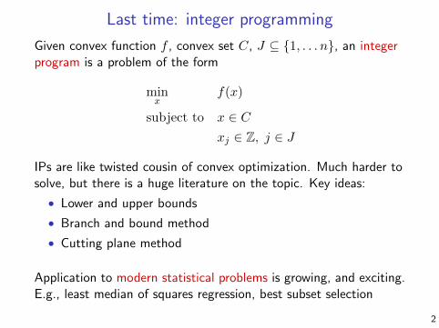
Last time: integer programming

Given convex function f , convex set C, J ⊆ 1, . . . n, an integerprogram is a problem of the form

minx

f(x)

subject to x ∈ Cxj ∈ Z, j ∈ J

IPs are like twisted cousin of convex optimization. Much harder tosolve, but there is a huge literature on the topic. Key ideas:

• Lower and upper bounds

• Branch and bound method

• Cutting plane method

Application to modern statistical problems is growing, and exciting.E.g., least median of squares regression, best subset selection

2

My soap box

Recently, it’s been said that statisticians should pay more attentionto IPs. I agree

But just because we can solve a nonconvex problem by formulatingit as IP, doesn’t mean we should prefer its solution over that fromrelated convex program

• The lasso is not a heuristic for best subset selection

• It’s an estimator, with its own properties

• An `1 penalty shrinks coefficients (unlike `0); this can hurt orhelp, depending on the situation

• Even if we could always solve best subset selection efficiently,it would be unwise to think that we should always prefer it

Optimizers should be more aware of the bias-variance tradeoff

3

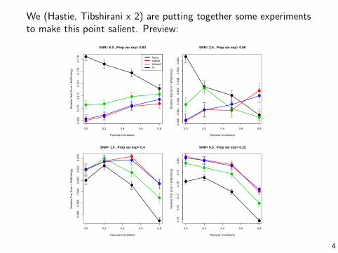
We (Hastie, Tibshirani x 2) are putting together some experimentsto make this point salient. Preview:

0.0 0.2 0.4 0.6 0.8

0.16

80.

170

0.17

20.

174

0.17

60.

178

SNR= 6.0 , Prop var exp= 0.83

Pairwise Correlation

Rel

ativ

e Te

st E

rror

= M

SE

/Var

(y)

lassosubsetrelaxedfs

0.0 0.2 0.4 0.6 0.8

0.34

00.

342

0.34

40.

346

0.34

80.

350

0.35

2

SNR= 2.5 , Prop var exp= 0.66

Pairwise Correlation

Rel

ativ

e Te

st E

rror

= M

SE

/Var

(y)

0.0 0.2 0.4 0.6 0.8

0.58

00.

585

0.59

00.

595

0.60

00.

605

SNR= 1.0 , Prop var exp= 0.4

Pairwise Correlation

Rel

ativ

e Te

st E

rror

= M

SE

/Var

(y)

0.0 0.2 0.4 0.6 0.8

0.75

0.76

0.77

0.78

0.79

0.80

SNR= 0.5 , Prop var exp= 0.22

Pairwise Correlation

Rel

ativ

e Te

st E

rror

= M

SE

/Var

(y)

4

Outline

Today:

• Convex versus nonconvex?

• Classical nonconvex problems

• Eigen problems

• Graph problems

• Nonconvex proximal operators

• Discrete problems

• Infinite-dimensional problems

• Statistical problems

• Miscellaneous

5

Beyond the tip?

6

Some takeaway points

• If possible, formulate task in terms of convex optimization —typically easier to solve, easier to analyze

• Nonconvex does not necessarily mean nonscientific! However,statistically, it can often mean high(er) variance

• This is true both intrinsically, and because we can rarely solvenonconvex problems (to global optimality)

• In more cases than you might expect, nonconvex problems canbe solved exactly (to global optimality)

7

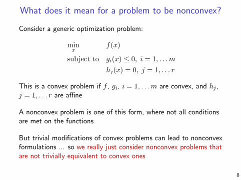
What does it mean for a problem to be nonconvex?

Consider a generic optimization problem:

minx

f(x)

subject to gi(x) ≤ 0, i = 1, . . .m

hj(x) = 0, j = 1, . . . r

This is a convex problem if f , gi, i = 1, . . .m are convex, and hj ,j = 1, . . . r are affine

A nonconvex problem is one of this form, where not all conditionsare met on the functions

But trivial modifications of convex problems can lead to nonconvexformulations ... so we really just consider nonconvex problems thatare not trivially equivalent to convex ones

8

What does it mean to solve a nonconvex problem?

Nonconvex problems can have local minima, i.e., there can exist afeasible x such that

f(y) ≥ f(x) for all feasible y such that ‖x− y‖2 ≤ R

but x is still not globally optimal. (Note: we proved that this couldnot happen for convex problems)

Hence by solving a nonconvex problem, we mean finding the globalminimizer

We also implicitly mean doing it efficiently, i.e., in polynomial time

9

Addendum

This is really about putting together a list of interesting problems,that are suprisingly tractable ... so there will be exceptions aboutnonconvexity and/or requiring exact global optima

(Also, I’m sure that there are many more examples out there thatI’m missing, so I invite you to give me ideas / contribute!)

10

Classical nonconvex problems

11

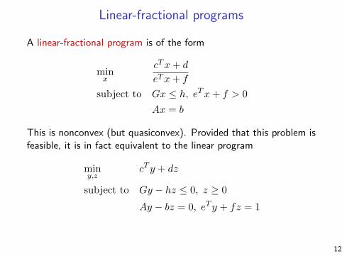
Linear-fractional programs

A linear-fractional program is of the form

minx

cTx+ d

eTx+ f

subject to Gx ≤ h, eTx+ f > 0

Ax = b

This is nonconvex (but quasiconvex). Provided that this problem isfeasible, it is in fact equivalent to the linear program

miny,z

cT y + dz

subject to Gy − hz ≤ 0, z ≥ 0

Ay − bz = 0, eT y + fz = 1

12

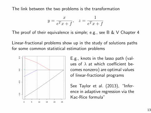
The link between the two problems is the transformation

y =x

eTx+ f, z =

1

eTx+ f

The proof of their equivalence is simple; e.g., see B & V Chapter 4

Linear-fractional problems show up in the study of solutions pathsfor some common statistical estimation problems

0 5 10 15 20 25

−1.

0−

0.5

0.0

0.5

E.g., knots in the lasso path (val-ues of λ at which coefficient be-comes nonzero) are optimal valuesof linear-fractional programs

See Taylor et al. (2013), “Infer-ence in adaptive regression via theKac-Rice formula”

13

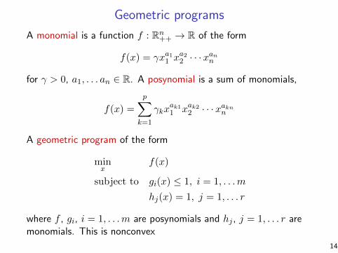
Geometric programs

A monomial is a function f : Rn++ → R of the form

f(x) = γxa11 xa22 · · ·xann

for γ > 0, a1, . . . an ∈ R. A posynomial is a sum of monomials,

f(x) =

p∑

k=1

γkxak11 xak22 · · ·xaknn

A geometric program of the form

minx

f(x)

subject to gi(x) ≤ 1, i = 1, . . .m

hj(x) = 1, j = 1, . . . r

where f , gi, i = 1, . . .m are posynomials and hj , j = 1, . . . r aremonomials. This is nonconvex

14

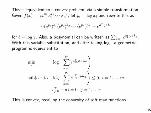
This is equivalent to a convex problem, via a simple transformation.Given f(x) = γxa11 x

a22 · · ·xann , let yi = log xi and rewrite this as

γ(ey1)a1(ey2)a2 · · · (eyn)an = eaT y+b

for b = log γ. Also, a posynomial can be written as∑p

k=1 eaTk y+bk .

With this variable substitution, and after taking logs, a geometricprogram is equivalent to

miny

log

(p0∑

k=1

eaT0ky+b0k

)

subject to log

(pi∑

k=1

eaTiky+bik

)≤ 0, i = 1, . . .m

cTj y + dj = 0, j = 1, . . . r

This is convex, recalling the convexity of soft max functions

15

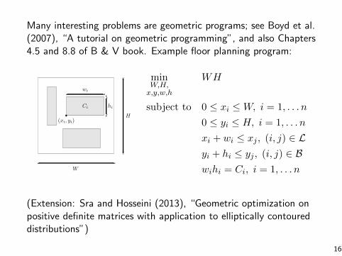
Many interesting problems are geometric programs; see Boyd et al.(2007), “A tutorial on geometric programming”, and also Chapters4.5 and 8.8 of B & V book. Example floor planning program:

8.8 Floor planning 439

W

H

hi

wi

(xi, yi)

Ci

Figure 8.18 Floor planning problem. Non-overlapping rectangular cells areplaced in a rectangle with width W , height H, and lower left corner at (0, 0).The ith cell is specified by its width wi, height hi, and the coordinates of itslower left corner, (xi, yi).

We also require that the cells do not overlap, except possibly on their boundaries:

int (Ci ∩ Cj) = ∅ for i = j.

(It is also possible to require a positive minimum clearance between the cells.) Thenon-overlap constraint int(Ci ∩ Cj) = ∅ holds if and only if for i = j,

Ci is left of Cj , or Ci is right of Cj , or Ci is below Cj , or Ci is above Cj .

These four geometric conditions correspond to the inequalities

xi + wi ≤ xj , or xj + wj ≤ xi, or yi + hj ≤ yj , or yj + hi ≤ yi, (8.32)

at least one of which must hold for each i = j. Note the combinatorial nature ofthese constraints: for each pair i = j, at least one of the four inequalities abovemust hold.

8.8.1 Relative positioning constraints

The idea of relative positioning constraints is to specify, for each pair of cells,one of the four possible relative positioning conditions, i.e., left, right, above, orbelow. One simple method to specify these constraints is to give two relations on1, . . . , N: L (meaning ‘left of’) and B (meaning ‘below’). We then impose theconstraint that Ci is to the left of Cj if (i, j) ∈ L, and Ci is below Cj if (i, j) ∈ B.This yields the constraints

xi + wi ≤ xj for (i, j) ∈ L, yi + hi ≤ yj for (i, j) ∈ B, (8.33)

minW,H,x,y,w,h

WH

subject to 0 ≤ xi ≤W, i = 1, . . . n

0 ≤ yi ≤ H, i = 1, . . . n

xi + wi ≤ xj , (i, j) ∈ Lyi + hi ≤ yj , (i, j) ∈ Bwihi = Ci, i = 1, . . . n

(Extension: Sra and Hosseini (2013), “Geometric optimization onpositive definite matrices with application to elliptically contoureddistributions”)

16

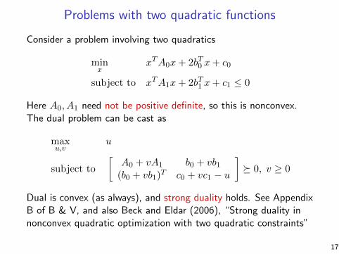
Problems with two quadratic functions

Consider a problem involving two quadratics

minx

xTA0x+ 2bT0 x+ c0

subject to xTA1x+ 2bT1 x+ c1 ≤ 0

Here A0, A1 need not be positive definite, so this is nonconvex.The dual problem can be cast as

maxu,v

u

subject to

[A0 + vA1 b0 + vb1

(b0 + vb1)T c0 + vc1 − u

] 0, v ≥ 0

Dual is convex (as always), and strong duality holds. See AppendixB of B & V, and also Beck and Eldar (2006), “Strong duality innonconvex quadratic optimization with two quadratic constraints”

17

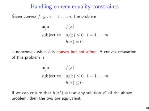
Handling convex equality constraints

Given convex f , gi, i = 1, . . .m, the problem

minx

f(x)

subject to gi(x) ≤ 0, i = 1, . . .m

h(x) = 0

is nonconvex when h is convex but not affine. A convex relaxationof this problem is

minx

f(x)

subject to gi(x) ≤ 0, i = 1, . . .m

h(x) ≤ 0

If we can ensure that h(x∗) = 0 at any solution x∗ of the aboveproblem, then the two are equivalent

18

From B & V Exercises 4.6 and 4.58, e.g., consider the maximumutility problem

maxx,b

T∑

t=1

αtu(xt)

subject to bt+1 = bt + f(bt)− xt, t = 1, . . . T

0 ≤ xt ≤ bt, t = 1, . . . T

where b0 ≥ 0 is fixed. Interpretation: xt is the amount spent ofyour total available money bt at time t; concave function u givesutility, concave function f measures investment return

This is not a convex problem, because of the equality constraint;but can relax to

bt+1 ≤ bt + f(bt)− xt, t = 0, . . . T

without changing solution (think about throwing out money)

19

Convexifying constraint sets

Given nonconvex set C, consider the nonconvex problem

minx

cTx subject to x ∈ C

Due to linearity of objective, this is equivalent to convex problem

minx

cTx subject to x ∈ conv(C)

Proof: let f? be optimal value in first problem, x? be solution insecond. Then x? =

∑i aixi where xi ∈ C, ai ≥ 0, and

∑i ai = 1.

Note f? ≥ cTx? =∑

i aicTxi ≥

∑i aif

? = f?. Thus all xi mustbe optimal for first problem

But note that the convex problem is not necessarily easy! Could bevery hard to even form conv(C) (recall the cutting plane methodfor integer programming)

20

Eigen problems

21

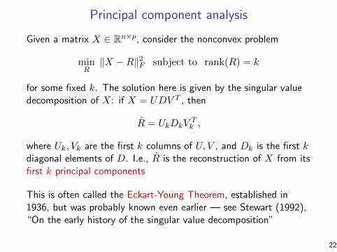
Principal component analysis

Given a matrix X ∈ Rn×p, consider the nonconvex problem

minR‖X −R‖2F subject to rank(R) = k

for some fixed k. The solution here is given by the singular valuedecomposition of X: if X = UDV T , then

R = UkDkVTk ,

where Uk, Vk are the first k columns of U, V , and Dk is the first kdiagonal elements of D. I.e., R is the reconstruction of X from itsfirst k principal components

This is often called the Eckart-Young Theorem, established in1936, but was probably known even earlier — see Stewart (1992),“On the early history of the singular value decomposition”

22

Fantope

Another characterization of the SVD is via the following nonconvexproblem, given X ∈ Rn×p:

minZ∈Sp

‖X −XZ‖2F subject to rank(Z) = k, Z projection

⇐⇒ maxZ∈Sp

〈XTX,Z〉 subject to rank(Z) = k, Z projection

The solution here is Z = VkVTk , where the columns of Vk ∈ Rp×k

give the first k eigenvectors of XTX

This is equivalent to a convex problem. Express constraint set C as

C =Z ∈ Sp : rank(Z) = k, Z is a projection

=Z ∈ Sp : λi(Z) ∈ 0, 1, i = 1, . . . p, tr(Z) = k

23

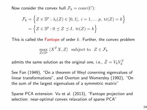
Now consider the convex hull Fk = conv(C):

Fk =Z ∈ Sp : λi(Z) ∈ [0, 1], i = 1, . . . p, tr(Z) = k

=Z ∈ Sp : 0 Z I, tr(Z) = k

This is called the Fantope of order k. Further, the convex problem

maxZ∈Sp

〈XTX,Z〉 subject to Z ∈ Fk

admits the same solution as the original one, i.e., Z = VkVTk

See Fan (1949), “On a theorem of Weyl conerning eigenvalues oflinear transformations”, and Overton and Womersley (1992), “Onthe sum of the largest eigenvalues of a symmetric matrix”

Sparse PCA extension: Vu et al. (2013), “Fantope projection andselection: near-optimal convex relaxation of sparse PCA”

24

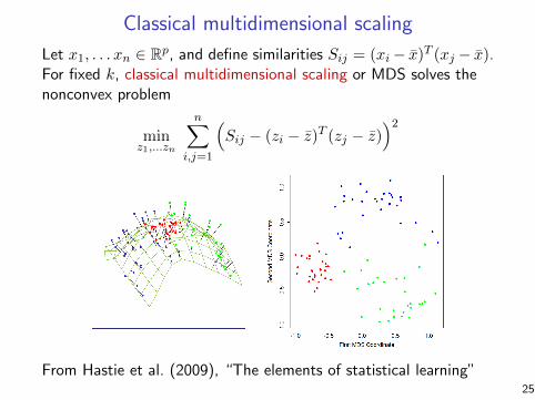
Classical multidimensional scaling

Let x1, . . . xn ∈ Rp, and define similarities Sij = (xi− x)T (xj − x).For fixed k, classical multidimensional scaling or MDS solves thenonconvex problem

minz1,...zn

n∑

i,j=1

(Sij − (zi − z)T (zj − z)

)2

From Hastie et al. (2009), “The elements of statistical learning”25

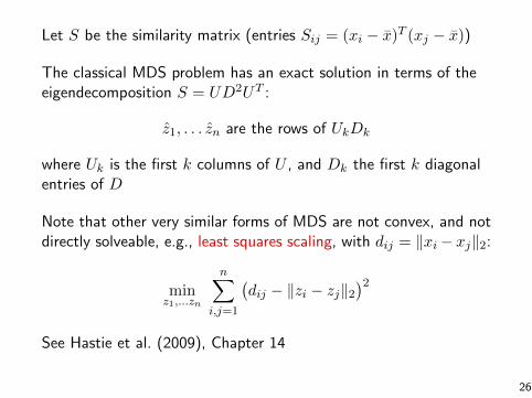
Let S be the similarity matrix (entries Sij = (xi − x)T (xj − x))

The classical MDS problem has an exact solution in terms of theeigendecomposition S = UD2UT :

z1, . . . zn are the rows of UkDk

where Uk is the first k columns of U , and Dk the first k diagonalentries of D

Note that other very similar forms of MDS are not convex, and notdirectly solveable, e.g., least squares scaling, with dij = ‖xi− xj‖2:

minz1,...zn

n∑

i,j=1

(dij − ‖zi − zj‖2

)2

See Hastie et al. (2009), Chapter 14

26

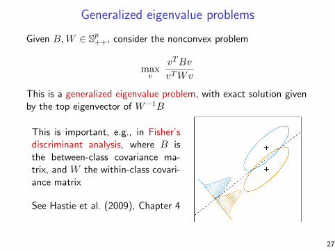
Generalized eigenvalue problems

Given B,W ∈ Sp++, consider the nonconvex problem

maxv

vTBv

vTWv

This is a generalized eigenvalue problem, with exact solution givenby the top eigenvector of W−1B

This is important, e.g., in Fisher’sdiscriminant analysis, where B isthe between-class covariance ma-trix, and W the within-class covari-ance matrix

See Hastie et al. (2009), Chapter 4

27

Graph problems

28

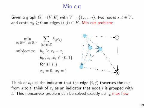
Min cut

Given a graph G = (V,E) with V = 1, . . . n, two nodes s, t ∈ V ,and costs cij ≥ 0 on edges (i, j) ∈ E. Min cut problem:

minb∈R|E|, x∈R|V |

∑

(i,j)∈Ebijcij

subject to bij ≥ xi − xjbij , xi, xj ∈ 0, 1for all i, j,

xs = 0, xt = 1

Think of bij as the indicator that the edge (i, j) traverses the cutfrom s to t; think of xi as an indicator that node i is grouped witht. This nonconvex problem can be solved exactly using max flow

29

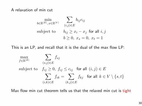
A relaxation of min cut

minb∈R|E|, x∈R|V |

∑

(i,j)∈Ebijcij

subject to bij ≥ xi − xj for all i, j

b ≥ 0, xs = 0, xt = 1

This is an LP, and recall that it is the dual of the max flow LP:

maxf∈R|E|

∑

(s,j)∈Efsj

subject to fij ≥ 0, fij ≤ cij for all (i, j) ∈ E∑

(i,k)∈Efik =

∑

(k,j)∈Efkj for all k ∈ V \ s, t

Max flow min cut theorem tells us that the relaxed min cut is tight

30

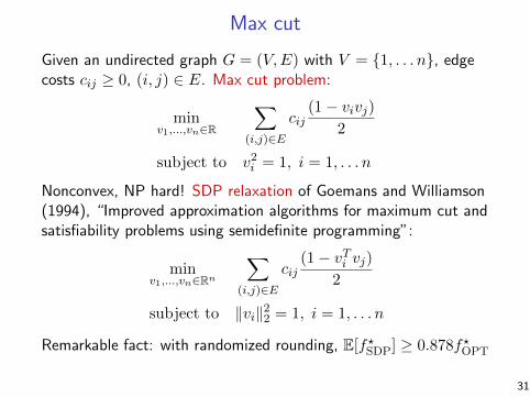
Max cut

Given an undirected graph G = (V,E) with V = 1, . . . n, edgecosts cij ≥ 0, (i, j) ∈ E. Max cut problem:

minv1,...,vn∈R

∑

(i,j)∈Ecij

(1− vivj)2

subject to v2i = 1, i = 1, . . . n

Nonconvex, NP hard! SDP relaxation of Goemans and Williamson(1994), “Improved approximation algorithms for maximum cut andsatisfiability problems using semidefinite programming”:

minv1,...,vn∈Rn

∑

(i,j)∈Ecij

(1− vTi vj)2

subject to ‖vi‖22 = 1, i = 1, . . . n

Remarkable fact: with randomized rounding, E[f?SDP] ≥ 0.878f?OPT

31

Nonconvex proximal operators

32

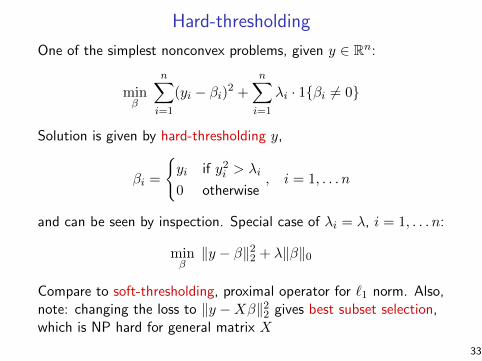
Hard-thresholding

One of the simplest nonconvex problems, given y ∈ Rn:

minβ

n∑

i=1

(yi − βi)2 +

n∑

i=1

λi · 1βi 6= 0

Solution is given by hard-thresholding y,

βi =

yi if y2i > λi

0 otherwise, i = 1, . . . n

and can be seen by inspection. Special case of λi = λ, i = 1, . . . n:

minβ‖y − β‖22 + λ‖β‖0

Compare to soft-thresholding, proximal operator for `1 norm. Also,note: changing the loss to ‖y −Xβ‖22 gives best subset selection,which is NP hard for general matrix X

33

Potts minimization

Consider 1d segmentation problem, also called Potts minimization:

minβ

n∑

i=1

(yi − βi)2 + λ

n−1∑

i=1

1βi 6= βi+1

Nonconvex, but solveable by dynamic programming, in two ways:Bellman (1961), “On the approximation of curves by line segmentsusing dynamic programming”, and Johnson (2013) “A dynamicprogramming algorithm for the fused lasso and L0-segmentation”

Johnson: more efficient, Bellman:more general

Worst-case O(n2), but with prac-tical performance more like O(n)

34

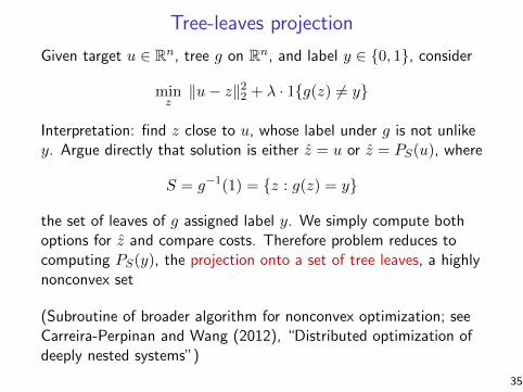
Tree-leaves projection

Given target u ∈ Rn, tree g on Rn, and label y ∈ 0, 1, consider

minz‖u− z‖22 + λ · 1g(z) 6= y

Interpretation: find z close to u, whose label under g is not unlikey. Argue directly that solution is either z = u or z = PS(u), where

S = g−1(1) = z : g(z) = y

the set of leaves of g assigned label y. We simply compute bothoptions for z and compare costs. Therefore problem reduces tocomputing PS(y), the projection onto a set of tree leaves, a highlynonconvex set

(Subroutine of broader algorithm for nonconvex optimization; seeCarreira-Perpinan and Wang (2012), “Distributed optimization ofdeeply nested systems”)

35

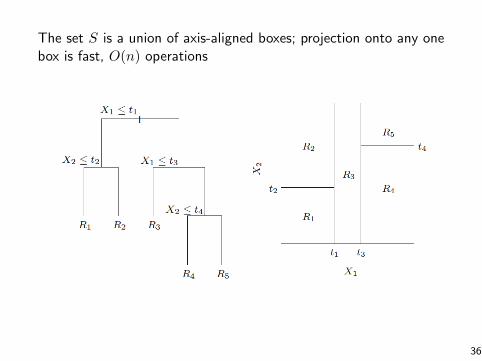
The set S is a union of axis-aligned boxes; projection onto any onebox is fast, O(n) operations

36

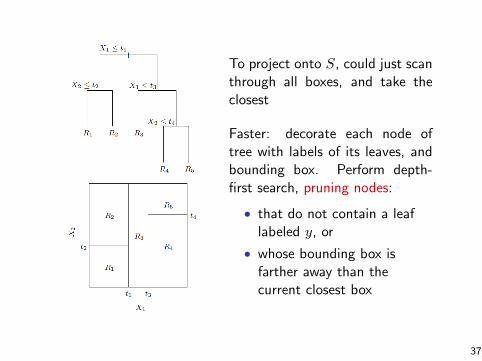
To project onto S, could just scanthrough all boxes, and take theclosest

Faster: decorate each node oftree with labels of its leaves, andbounding box. Perform depth-first search, pruning nodes:

• that do not contain a leaflabeled y, or

• whose bounding box isfarther away than thecurrent closest box

37

Discrete problems

38

Binary graph segmentation

Given y ∈ Rn, undirected graph G = (V,E) with V = 1, . . . n,consider binary graph segmentation:

minβ∈0,1n

n∑

i=1

(yi − βi)2 +∑

(i,j)∈Eλij · 1βi 6= βj

Nonconvex, but simple manipulation delivers the equivalent form

maxA⊆1,...n

∑

i∈Aai +

∑

j∈Acbj −

∑

(i,j)∈E, |A∩i,j|=1

λij

which is a segmentation problem that can be solved exactly usingmin cut/max flow. E.g., Kleinberg and Tardos (2005), “Algorithmdesign”, Chapter 7

39

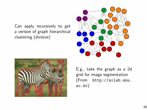
Can apply recursively to geta verison of graph hierarchicalclustering (divisive)

E.g., take the graph as a 2dgrid for image segmentation(From http://ailab.snu.

ac.kr)

40

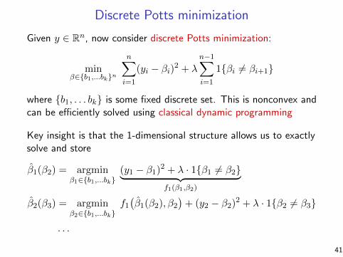
Discrete Potts minimization

Given y ∈ Rn, now consider discrete Potts minimization:

minβ∈b1,...bkn

n∑

i=1

(yi − βi)2 + λ

n−1∑

i=1

1βi 6= βi+1

where b1, . . . bk is some fixed discrete set. This is nonconvex andcan be efficiently solved using classical dynamic programming

Key insight is that the 1-dimensional structure allows us to exactlysolve and store

β1(β2) = argminβ1∈b1,...bk

(y1 − β1)2 + λ · 1β1 6= β2︸ ︷︷ ︸f1(β1,β2)

β2(β3) = argminβ2∈b1,...bk

f1(β1(β2), β2

)+ (y2 − β2)2 + λ · 1β2 6= β3

. . .

41

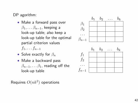
DP agorithm:

• Make a forward pass overβ1, . . . βn−1, keeping alook-up table; also keep alook-up table for the optimalpartial criterion valuesf1, . . . fn−1

• Solve exactly for βn

• Make a backward passβn−1, . . . β1, reading off thelook-up table

b1 b2 . . . bkβ1β2. . .βn−1

b1 b2 . . . bkf1f2. . .fn−1

Requires O(nk2) operations

42

Nearly optimal K-means

Given data points x1, . . . xn ∈ Rp, the K-means problem is

minc1,...cK

n∑

i=1

mink=1,...K

‖xi − ck‖22︸ ︷︷ ︸

f(c1,...cK)

This is nonconvex, NP hard, and it is usually approximately solvedusing Lloyd’s algorithm, run many times, with random starts

Careful choice of starting positions makes a big impact: if we runLloyd’s algorithm once, starting at c1 = s1, . . . cK = sK , for special(random) s1, . . . sK , then we get estimates c1, . . . cK with

E[f(c1, . . . cK)

]≤ 8(log k + 2) · min

c1,...cK∈Rpf(c1, . . . cK)

43

See Arthur and Vassilvitskii (2007), “k-means++: The advantagesof careful seeding”. Their construction of s1, . . . sK is simple:

• Begin by choosing s1 uniformly at random among x1, . . . xn

• Compute squared distances

d2i = ‖xi − s1‖22

for all points i not chosen, and choose s2 by drawing from theremaining points, with probability weights d2i /

∑j d

2j

• Recompute the squared distances as

d2i = min‖xi − s1‖22, ‖xi − s2‖22

and choose s3 according to the same recipe

• And so on, until all of s1, . . . sK are chosen

44

Infinite-dimensional problems

45

Smoothing splines

Given pairs (xi, yi) ∈ R× R, i = 1, . . . n, smoothing spline solves

minf

n∑

i=1

(yi − f(xi)

)2+ λ

∫ (f ′′(t)

)2dt

Optimization domain: all functions f such that∫

(f ′′(t))2 dt <∞,infinite-dimensional set

Can show that the solution f to the above problem is unique, andgiven by natural cubic spline, that has knots at x1, . . . xn. (Proof:use integration by parts.) Hence we can parametrize by

f =

n∑

j=1

θjηj

where η1, . . . ηn are natural cubic spline basis functions. Task nowis to solve for coefficients θ ∈ Rn

46

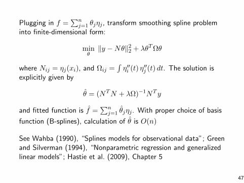
Plugging in f =∑n

j=1 θjηj , transform smoothing spline probleminto finite-dimensional form:

minθ‖y −Nθ‖22 + λθTΩθ

where Nij = ηj(xi), and Ωij =∫η′′i (t) η′′j (t) dt. The solution is

explicitly given by

θ = (NTN + λΩ)−1NT y

and fitted function is f =∑n

j=1 θjηj . With proper choice of basis

function (B-splines), calculation of θ is O(n)

See Wahba (1990), “Splines models for observational data”; Greenand Silverman (1994), “Nonparametric regression and generalizedlinear models”; Hastie et al. (2009), Chapter 5

47

Locally adaptive regression splines

Given same setup, (cubic) locally adaptive regression spline solves

minf

n∑

i=1

(yi − f(xi)

)2+ λ · TV(f ′′′)

Optimization domain: all functions f with TV(f ′′′) <∞, which isagain infinite-dimensional

Similar to before, can show that the solution f to above problem isa cubic spline, but two key differences:

• Can have any number of knots ≤ n− 4 (tuned by λ)

• Knots do not necessarily lie at input points x1, . . . xn!

Details in Mammen and van de Geer (1997), “Locally adaptiveregression splines”. Summary: these are statistically more adaptivebut computationally more challenging than smoothing splines

48

Smoothing spline Locally adaptive spline(easier to compute) (more adaptive)

Finite-dimensional approximation is given in Mammen and van deGeer (1997), and a much faster approximation in Tibshirani (2014),“Adaptive piecewise polynomial estimation via trend filtering”

49

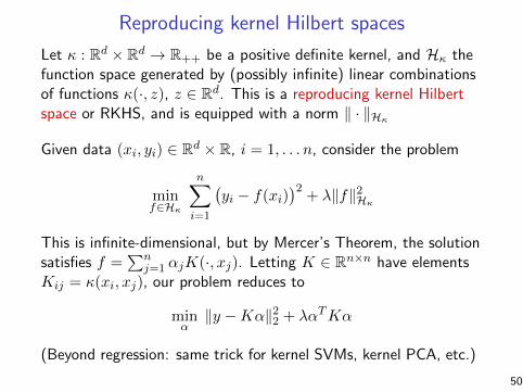
Reproducing kernel Hilbert spaces

Let κ : Rd × Rd → R++ be a positive definite kernel, and Hκ thefunction space generated by (possibly infinite) linear combinationsof functions κ(·, z), z ∈ Rd. This is a reproducing kernel Hilbertspace or RKHS, and is equipped with a norm ‖ · ‖Hκ

Given data (xi, yi) ∈ Rd × R, i = 1, . . . n, consider the problem

minf∈Hκ

n∑

i=1

(yi − f(xi)

)2+ λ‖f‖2Hκ

This is infinite-dimensional, but by Mercer’s Theorem, the solutionsatisfies f =

∑nj=1 αjK(·, xj). Letting K ∈ Rn×n have elements

Kij = κ(xi, xj), our problem reduces to

minα‖y −Kα‖22 + λαTKα

(Beyond regression: same trick for kernel SVMs, kernel PCA, etc.)

50

Statistical problems

51

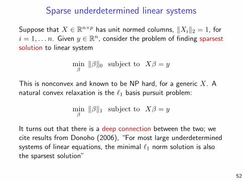
Sparse underdetermined linear systems

Suppose that X ∈ Rn×p has unit normed columns, ‖Xi‖2 = 1, fori = 1, . . . n. Given y ∈ Rn, consider the problem of finding sparsestsolution to linear system

minβ‖β‖0 subject to Xβ = y

This is nonconvex and known to be NP hard, for a generic X. Anatural convex relaxation is the `1 basis pursuit problem:

minβ‖β‖1 subject to Xβ = y

It turns out that there is a deep connection between the two; wecite results from Donoho (2006), “For most large underdeterminedsystems of linear equations, the minimal `1 norm solution is alsothe sparsest solution”

52

As n, p grow large, p > n, there exists a threshold ρ (depending onthe ratio p/n), such that for most matrices X, the following holds.If we solve the `1 problem and find a solution with:

• fewer than ρn nonzero components, then we must have foundthe unique solution of the `0 problem

• greater than ρn nonzero components, then there is no solutionof the linear system with less than ρn nonzero components

Here “most” can be quantified precisely via a uniform probabilitymeasure over matrices X with unit norm columns

There is a large and fast-moving body of related literature. SeeDonoho et al. (2009), “Message-passing algorithms for compressedsensing” for a nice review

53

Exact low-rank matrix completion

Given a matrix Y ∈ Rn×n, partially observed, over a set of indicesΩ ⊆ 1, . . . , n2. Consider the problem of finding the lowest-rankmatrix matching Y on the observed set

minB

rank(B) subject to Bij = Yij , (i, j) ∈ Ω

This is nonconvex. Natural convex relaxation:

minB‖B‖tr subject to Bij = Yij , (i, j) ∈ Ω

Under some assumptions, it can be shown that the solution to theconvex problem is exactly equal to the solution to the nonconvexproblem, with high probability over the sampling model

See, e.g., Candes and Recht (2008), “Exact matrix completion viaconvex optimization”, and many papers since

54

Miscellaneous

55

Curvature domination

Given convex f and nonconvex g, consider a problem

minx

f(x) + g(x)

For convex h, we can always rewrite this problem as

minx

f(x) + g(x)− h(x)︸ ︷︷ ︸F (x)

+ h(x)

Sometimes, can choose h to make F smooth and strictly convex!How? Prove that ∇2f(x) ∇2(h− g)(x) for all x

This is apparently an old idea. See Parekh and Selesnick (2015),“Convex fused lasso denoising with non-convex regularization andits use for pulse detection” and references therein. (Related ideason curvature domination from statistics: Zhang, Loh, Wainwright)

56

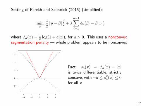
Setting of Parekh and Selesnick (2015) (simplified):

minβ

1

2‖y − β‖22 + λ

n−1∑

i=1

φa(βi − βi+1)

where φa(x) = 1a log(1 + a|x|), for a > 0. This uses a nonconvex

segmentation penalty — whole problem appears to be nonconvex

−4 −2 0 2 4

−1

01

23

Fact: sa(x) = φa(x) − |x|is twice differentiable, strictlyconcave, with −a ≤ s′′a(x) ≤ 0for all x

57

Rewrite problem (denoting by D the first difference operator) as

minβ

1

2‖y − β‖22 + λ

n−1∑

i=1

(φa([Dβ]i)− |[Dβ]i|

)

︸ ︷︷ ︸Fa(β)

+λ‖Dβ‖1

Now compute

∇2Fa(β) = I + λDTSa(Dβ)D

where Sa(x) = diag(s′′a(x1), . . . s′′a(xn−1)). Easy to check that

DTSa(Dβ)D −aDTD −4a

using our previous fact, and λmax(DTD) = 4. Thus Fa(β) — andour whole problem — is strictly convex provided 1− 4aλ > 0, i.e.,a < 1/(4λ)

58

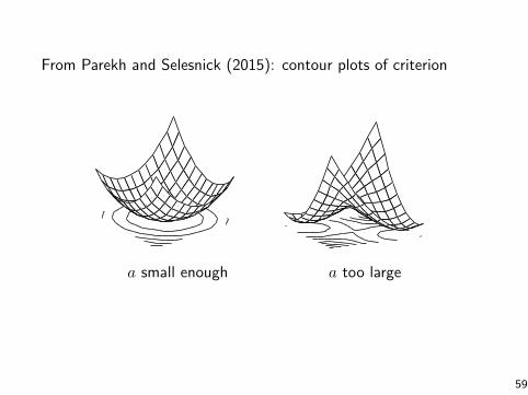
From Parekh and Selesnick (2015): contour plots of criterionIEEE SIGNAL PROCESSING IN MEDICINE AND BIOLOGY SYMPOSIUM, DECEMBER 2015. 3

(a) G(x),a0 = 1/2,a1 = 1/8 (b) G(x),a0 = 1/2,a1 = 1/3

Fig. 1. Surface plots illustrating the convexity condition. (a) The functionG(x) (15) is convex for a0 = 1/2 and a1 = 1/8. (b) The function G(x) isnot convex for a0 = 1/2 and a1 = 1/3 (these values violate Theorem 1).

For the strict convexity of G, we need to ensure that ∇2G ispositive definite. To this end, from the assumptions on φ, itfollows that

Γ(x; a0) ! −a0I, x ∈ RN . (18)

Moreover, we can write

DT Γ(Dx; a1)D ! −a1DT D (19)

≻ −4a1I. (20)

The inequality (20) is obtained using the eigenvalues1 of thematrix DT D. Using (16), (18) and (20), ∇2G ≻ 0 if

(1 − a0λ0 − 4a1λ1)I ! 0, (21)

or equivalently if,

1 − a0λ0 − 4a1λ1 " 0. (22)

From (11), (13) and (15) it is straighforward that

F (x) = G(x) + λ0∥x∥1 + λ1∥Dx∥1. (23)

Hence, F in (13) is strictly convex as long as the inequality(22) holds true (the function F is a sum of a strictly convexfunction G, the convex ℓ1 norm, and the convex TV penalty).

The following example illustrates the convexity condition(22) for N = 2. Let λ0 = λ1 = 1 and y = 0. As per Theorem1, the function G (by extension the function F ) is strictlyconvex if a0 + 4a1 # 1. Figure 1(a) shows the function Gwith the values a0 = 1/2 and a1 = 1/8. These values satisfyTheorem 1 and as a result the function G is strictly convex.On the other hand, Fig. 1(b) shows the function G when a0 =1/2 and a1 = 1/3. These values of a0 and a1 violate theTheorem 1; consequently the functionG is non-convex as seenin Fig. 1(b).The convexity condition given by Theorem 1 in (14) implies

that the values of a0 and a1 must lie on or below the line givenby a0λ1 + 4a1λ1 = 1. Figure 2 displays the values of a0 anda1 for which the function F is strictly convex. In order tomaximally induce sparsity, we choose the values of a0 anda1 on the line. Specifically, we propose to select a value of

1The eigenvalues of DT D are given by 2 − 2 cos(kπ/N) for k =0, . . . , N − 1 [30].

a0

a 1

Convex

Non−Convex

0 1/λ00

1/(4λ1)

Fig. 2. Region of convexity for the function F in (13). The function F isstrictly convex for any values of a0 and a1 inside the triangular region.

a0 ∈ (0, 1/λ) and set the value of a1 as

a1 =1 − a0λ0

4λ1. (24)

IV. OPTIMIZATION ALGORITHM

Due to Theorem 1, we can reliably obtain via convexoptimization the global minimum of (4) as long as the pa-rameters a0 and a1 are chosen to satisfy (14). We derive analgorithm for the proposed CNC fused lasso method using themajorization-minimization (MM) procedure [8], such that

xk+1 = arg minx

FM(x, xk), (25)

where FM denotes a majorizer of the function F in (4), andwhere k is the iteration index. The MM procedure guaranteesthat each iteration monotonically decreases the value of theobjective function F in (4). We use the absolute value functionand a linear function to majorize the non-convex penaltyfunction. With this particular choice of majorizer, each MMupdate iteration involves solving the ℓ1 FLSA problem (2).To derive a majorizer of the function φ, note that φ(x; a) =

s(x; a)+ |x|. As a result, it suffices to majorize the function swith a linear term in order to obtain a majorizer of the functionφ. Observe that since s is a concave function, the tangent lineto s at a point v always lies above the function s. Using thetangent line to the function s, a majorizer of the function φ isgiven by φM : R × R → R, defined as

φM(x, v; a) = |x| + s′(v; a)(x − v) + s(v; a), (26)

for x, v ∈ R. It follows straightforwardly that

φM(x, v; a) " φ(x; a), ∀x, v ∈ R, (27)φM(v, v; a) = φ(v; a), ∀v ∈ R. (28)

Figure 3(a) shows the absolute value function |x|. Thetwice continuously differentiable function s(x; a) is shown inFig. 3(b), along with the tangent line to s(x; a) at x = 1.Figure 3(c) shows the non-convex penalty function φ and itsmajorizer φM(x, v; s) given by (26). The majorizer is the sumof the absolute value function in Fig. 3(a) and the tangent lineto s(x; a) in Fig. 3(b).Using (27) and (28), we note that

!

n

φM"xn, vn; a

#"!

n

φ"xn; a

#, (29)

a small enough a too large

59

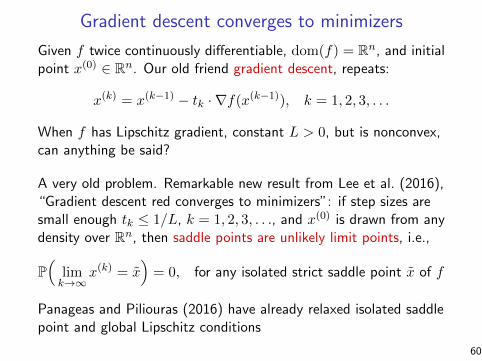
Gradient descent converges to minimizers

Given f twice continuously differentiable, dom(f) = Rn, and initialpoint x(0) ∈ Rn. Our old friend gradient descent, repeats:

x(k) = x(k−1) − tk · ∇f(x(k−1)), k = 1, 2, 3, . . .

When f has Lipschitz gradient, constant L > 0, but is nonconvex,can anything be said?

A very old problem. Remarkable new result from Lee et al. (2016),“Gradient descent red converges to minimizers”: if step sizes aresmall enough tk ≤ 1/L, k = 1, 2, 3, . . ., and x(0) is drawn from anydensity over Rn, then saddle points are unlikely limit points, i.e.,

P(

limk→∞

x(k) = x)

= 0, for any isolated strict saddle point x of f

Panageas and Piliouras (2016) have already relaxed isolated saddlepoint and global Lipschitz conditions

60