nonlinear algebraic multigrid for constrained solid ... · sand2006–2256 unlimited release...

SAND2006–2256

Unlimited Release

Printed April 2006

Nonlinear algebraic multigrid for constrained solid mechanics problemsusing Trilinos

Michael W. Gee

Computational Math & Algorithms

Sandia National Laboratories

PO Box 5800, Albuquerque, NM, 87185–1110

Ray S. Tuminaro

Computational Math & Algorithms

Sandia National Laboratories

PO Box 0969, Livermore, CA, 94551–0969

Key words nonlinear multigrid, algebraic multigrid, smoothed aggregation, nonlinear systems of equations,

full approximation scheme, nonlinear conjugate gradients, Newton’s method

Abstract

The application of the finite element method to nonlinear solid mechanics problems results in the neccessity

to repeatedly solve a large nonlinear set of equations. In this paper we limit ourself to problems arising in

constrained solid mechanics problems. It is common to apply some variant of Newton’s method or a Newton–

Krylov method to such problems. Often, an analytic Jacobian matrix is formed and used in the above mentioned

methods. However, if no analytic Jacobian is given, Newton methods might not be the method of choice. Here,

we focus on a variational nonlinear multigrid approach that adopts the smoothed aggregation algebraic multi-

grid method to generate a hierachy of coarse grids in a purely algebraic manner. We use preconditioned nonlin-

ear conjugent gradient methods and/or quasi–Newton methods as nonlinear smoothers on fine and coarse grids.

In addition we discuss the possibility to augment this basic algorithm with an automatically generated Jacobian

by applying a block colored finite differencing scheme. After outlining the fundamental algorithms we give

some examples and provide documentation for the parallel implementation of the described method within the

Trilinos framework.

Acknowledgment

This work was partially funded by the Department of Energy Office of Science MICS program at Sandia Nation-

al Laboratory. Sandia is a multiprogram laboratory operated by Sandia Corporation, a Lockheed Martin Compa-

ny, for the United Stated Department of Energy’s National Nuclear Security Administration under contract DE–

AC04–94AL85000.

M.W. Gee, R.S. Tuminaro

2

(page intentionally left blank)


3

1 Intr oduction and problem definition

The application of the finite element method to nonlinear solid mechanics problems results

in the necessity to repeatedly solve a nonlinear function

F(x) � 0 , (1)

where F : �N � �N usually is a vector of residual forces and x is a vector of primal variables

such as nodal velocities or displacements. In this paper we limit ourself to problems arising

in (contrained) nonlinear solid mechanics though the given methods and algorithms might be

applicable to other types of nonlinear problems as well.

It is common to apply some variant of Newton’s method or some kind of Newton–Krylov

method to Eq. (1). With the exception of matrix–free Newton type algorithms, if F is differen-

tiable at x, a Jacobian

J(x) � �Jij�(x) ��Fi�xj

(x) (2)

is formed and used in the Newton– or Newton–Krylov type algorithm [14]. This differentiation

can be performed analytically in some cases, or the Jacobian can be formed by a numerical

finite difference approximation to the differentiation. Newton type methods in general have

very good convergence characterictics but are not guaranteed to converge. The initial estimate

x0 has to be sufficiently close to the solution and the Jacobian J has to be a sufficiently good

approximation to Eq. (2). Here, we focus on cases were either one or both of these conditions

are not met so that Newton’s method might not be an appropiate choice.

Besides these Newton type methods, there exist several other solution approaches as e.g.

the nonlinear Gauss–Seidel algorithm [6], preconditioned nonlinear conjugate gradient meth-

od (nonlinear CG) [2] or nonlinear multigrid schemes [3],[6].

We focus on a variational nonlinear multigrid approach called the full approximation

scheme (FAS) that adopts a smoothed aggregation algebraic multigrid method [18],[19],[20]

to create prolongation and restriction operators between grids in a purely algebraic manner.

No coarse grid discretizations of the underlying problem have to be provided. We use nonlinear

CG and/or quasi–Newton methods as nonlinear smoothers and approximate nonlinear solvers

on fine and coarse grids.

In addition we discuss the possibility to augment this basic algorithm with an automatically

generated Jacobian by applying a block colored finite difference scheme. With this capability

inside the nonlinear solver, the underlying application does not have to provide any Jacobian

to the multigrid algorithm. The algorithm is therefore suitable to use in applications that merely

have functionality to evaluate residuals at a given current solution state as would usually be

the case in purely explicit time integration codes.


4

Underlying theory and algorithms are discussed briefly in this article. The emphasis lies on

the usage of the implementation of the proposed algorithm in parallel within the software proj-

ect Trilinos [9] and on the discussion of the several method variants that can be used. We pro-

vide two examples comparing several choices.

The implementation makes use of several of Trilinos’ subpackages, most importantly the

algebraic multigrid package ML [15] and the nonlinear solver package NOX [16]. The present-

ed method is implemented in ML and uses its algebraic multigrid hierarchy. Nonlinear smooth-

ing and solution methods as well as the interface to an underlying application code are derived

from the NOX package.

This article is organized as follows. In Section 2 through Section 6 we present the proposed

nonlinear multigrid algorithm and pay special attention to its building blocks. In Section 7 the

usage of the method for problems with constraints is discussed and in Section 8 two examples

are given. Section 9 serves as a detailed documentation of the implementation of the method

and we conclude in Section 10.

2 Smoothed aggregation multigrid (SA)

A multigrid solver tries to approximate the original PDE problem of interest on a hierarchy

of grids and uses approximate solutions from coarse grids to accelerate the convergence on the

finest grid (which is the one of interest). To do so, a basic – in this case nonlinear – iterative

method has to be applied on each grid which effectively smooths out the error associated with

the current approximate solution on that grid.

The prolongation P and restriction R (operators that transfer solutions, residuals and

corrections from coarse to fine grids and vice versa, respectively) are the key ingredient and

are determined by the smoothed aggregation method, for details see [18],[19],[20]. The user

does not need to supply any hierarchy of coarse discretizations. However, it is advantageous

to supply some extra information about the problem, namely the kernel of the fine grid Jaco-

bian neglecting any Dirichlet boundary conditions. In the case of 3D–elasticity, the kernel con-

sists of six vectors describing the rigid body modes of the object of interest neglecting Dirichlet

boundary conditions. Computing these rigid body modes is not part of the presented imple-

mentation though details on how to compute them from nodal coordinates of the fine grid are

given in Section 9.2. The actual fine grid Jacobian is not needed to compute rigid body modes.

The implementation of the presented method also provides the capabilitiy to use an adaptive

smoothed aggregation procedure (�SA) [4] to identify additional near nullspace modes that

are not well captured by an existing multigrid hierarchy. These additional adaptively computed

modes are then added to the nullspace and this enriched near–nullspace is used to recompute

a multigrid hierachy with improved approximation and convergence properties.

As the adaptive smoothed aggregation multigrid procedure uses linear v–cycles to deter-


5

mine additional nullspace modes in the setup phase it is inexpensive compared to the actual

nonlinear iteration to be performed. It is therefore especially suitable to use in the nonlinear

setting, which does not always hold when used in linear multigrid methods. An example of

the adaptive smoothed aggregation approach is given in Section 8.3. The usage with the Trili-

nos implementation is described in Section 9.5.

Systems of equations resulting from finite element or other types of discretizations have a

sparse nodal block structure. When the underlying application retains degrees of freedom that

are prescribed by Dirichlet boundary condition within the system, the nodal block size is

constant throughout the system. However, some applications condense rows and columns as-

sociated with Dirichlet boundary condition from the system of equations resulting in a variable

block size. In those cases it is beneficial or even necessary to provide ML with additional infor-

mation about the block structure of the problem. ML supports variable blocked systems in the

generation of the multigrid hierarchy when sufficient information is provided. Building and

providing nodal block information as well as choosing the correct input parameters for ML is

described in Section 9.2.

3 Full approximation scheme (FAS)

The algorithm is described for a nonlinear multigrid V–cycle, which indicates the order that

coarse grids are visited and how they contribute to the solution. We use a classical full approxi-

mation scheme (FAS) [3],[6], that can be shown to reduce to a standard linear V–cycle in the

case that the nonlinear function F in Eq. (1) is in fact linear (see Remark 2).

In this paper sub– and superscripts ( )(l) , ( )(l) in parenthesis indicate a grid in the multigrid

hierarchy with l � 0 being the finest grid and L is the number of grids to be used. In the follow-

ing, the FAS V–cycle is explained as a 2–grid method choosing L � 2. Introducing an iterate

index k we can rewrite problem (1) on the fine grid as a series of iterates such that

Fk(0)�xk

(0)�� 0 . (3)

We introduce a nonlinear smoothing method S�1

(l)�Fk

(l), xk(l)� to be applied �1 times and obtain

the presmoothed fine grid iterate

x~ k(0) � S�1

(0)�Fk

(0), xk(0)� . (4)

Restricting the current solution vector x~ k(0) and the current residual Fk

(0)�x~ k

(0)� to the next

coarser grid yields

x(1) � R(1)(0)

x~ k(0) , F(1) � R(1)

(0)Fk

(0)�x~ k

(0)� . (5)

We omit the iterate index k on all coarse grid variables for clarity.

A modified coarse grid problem


6

F(1)x(1)

�F^

(1) x(1)

� F(1) � 0 (6)

is set up, where F(1) is obtained from Eq. (5) and

F^ x(1)� F

^ R(1)(0)

x~ k(0) . (7)

F(1) , F^

(1) are fixed quantities throughout the nonlinear smoothing iteration S�1

(1) applied to Eq.

(6)

x~ (1) � S�1

(1)F(1)�F

^(1) � F(1) , x(1) . (8)

The nonlinear function F(l) is evaluated in a variational way on all coarse grids l � 0. Specifi-

cally,

F(l)x(l)� R(l)(0)

F(0) P(0)(l)

x(l) , l � 0 , (9)

where P(j)(k)

prolongates from level k to level j and R(k)(j)

restricts from level j to level k. Specifi-

cally

P(0)(l)

� P(0)(1)

P(1)(2)

�� P(l�1)(l)

, (10)

R(l)(0)

� P(0)T(l)

, (11)

and R(l)T(l�1)

� P(l�1)(l)

correspond to the smoothed aggregation multigrid hierarchy discussed

in Section 2.

Remark 1: Operators P(0)(l)

, R(l)(0)

are never explicitly formed. Instead, Eq. (10) is applied.

Given the nonlinear smoothed coarse grid iterate x~ (1), a correction is calculated and added to

the current fine grid solution using the interpolation operator:

x~ k(0) � x~ k

(0)� P(0)(1)x~ (1)� x (1)

. (12)

Applying a postsmoothing step

xk�1(0) � S�2

(0)Fk

(0), x~ k(0) . (13)

�2 times finalizes the V–cycle. Fig. 1 gives the complete FAS solver scheme for the general

case L � 2. Therein, F(l) denotes the residual restricted to level l which remains unaltered

throughout the pre– and postsmoothing steps . The number of smoothing steps �1 and �2 can

be chosen independently on each grid. Choosing �1 � �2 on each grid results in a symmetric


7

V–cycle which is normally recommended for symmetric problems in the linear case. Choosing

�1 � �2 results in a nonsymmetric multigrid operator which can be comptetitive with respect

to performance in the nonlinear case.

FAS_Vcycle ( F(l) , x(l) , l )

F^

(l) � F(l)�x(l)

�Presmooth x(l) � S�1

(l)�F(l)�F

^(l) � F(l) , x(l)�

if l � L�1

FAS_Vcycle ( F(l�1) , x(l�1) , l � 1 )

x(l�1) � R(l�1)(l)

x(l)

F(l�1) � R(l�1)(l)

F(l)�x(l)

�

x(l) � x(l) � P(l)(l�1)

x(l�1)

endif

Postsmooth x(l) � S�1

(l)�F(l)�F

^(l) � F(l) , x(l)�

return

if l � 0

Presmooth x(l) � S�1

(l)�F(l) , x(l)

�else

endif

if l � 0


(l)�F(l) , x(l)

�else

endif

x(l) � x(l) � x(l)

Figure 1: FAS V–cycle as a solver

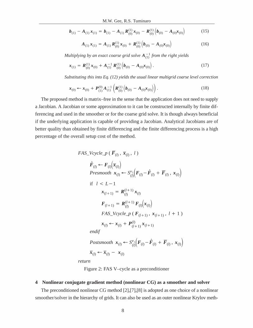
The full approximation scheme V–cycle can also be easily formulated as a preconditioner

to some outer nonlinear iteration, e.g. nonlinear CG. The V–cycle as a preconditioner is given

in Fig. 2. The ML implementation supports both versions.

Remark 2: When F(0) is linear and an exact coarse grid solve is used the algorithm correspondsto the usual multigrid scheme. In particular:

F(0) � b(0)� A(0)x(0) , F(1) � b(1) � A(1)x(1) . (14)

Substituting Eq. (14) into (6) we get


8

b(1)� A(1) x(1) � b(1)� A(1) R(1)(0)

x(0) � R(1)(0)�b(0) � A(0)x(0)� (15)

A(1) x(1) � A(1) R(1)(0)

x(0)� R(1)(0)�b(0)� A(0)x(0)� (16)

Multiplying by an exact coarse grid solve A�1(1) from the right yields

x(1) � R(1)(0)

x(0)� A�1(1) R(1)

(0)�b(0) � A(0)x(0)� . (17)

Substituting this into Eq. (12) yields the usual linear multigrid coarse level correction

x(0) � x(0)� P(0)(1)

A�1(1)�R(1)

(0)�b(0) � A(0)x(0)�� . (18)

The proposed method is matrix–free in the sense that the application does not need to supply

a Jacobian. A Jacobian or some approximation to it can be constructed internally by finite dif-

ferencing and used in the smoother or for the coarse grid solve. It is though always beneficial

if the underlying application is capable of providing a Jacobian. Analytical Jacobians are of

better quality than obtained by finite differencing and the finite differencing process is a high

percentage of the overall setup cost of the method.

FAS_Vcycle_p ( F(l) , x(l) , l )

F^

(l) � F(l)�x(l)

�Presmooth x(l) � S�1

(l)�F(l)�F

^(l) � F(l) , x(l)�

if l � L�1

FAS_Vcycle_p ( F(l�1) , x(l�1) , l � 1 )

x(l�1) � R(l�1)(l)

x(l)

F(l�1) � R(l�1)(l)

F(l)�x(l)

�

x(l) � x(l) � P(l)(l�1)

x(l�1)

endif


(l)�F(l)�F

^(l) � F(l) , x(l)�

return

x(l) � x(l) � x(l)

Figure 2: FAS V–cycle as a preconditioner

4 Nonlinear conjugate gradient method (nonlinear CG) as a smoother and solver

The preconditioned nonlinear CG method [2],[7],[8] is adopted as one choice of a nonlinear

smoother/solver in the hierarchy of grids. It can also be used as an outer nonlinear Krylov meth-


9

od to which the presented nonlinear algebraic multigrid is then applied as a nonlinear precondi-

tioner. Given the nonlinear problem Fk(l)�xk

(l)� from Eq. (1) on some grid (l) with k � 0,...,Niter

as iterate index a search direction

sk�1 � M�1 Fk , k � 0 , (19)

sk�1 � M�1 Fk � �k sk , k � 0 (20)

is computed omitting the grid identifier (l) for clarity, where M is a linear preconditioner and

�k results from the so called Polak–Ribière formula

�k �FkT M�1�Fk � Fk�1�

Fk�1T M�1 Fk�1. (21)

In the case �k � 0 the iteration is restarted using Eq. (19). A new iterate

xk�1 � xk � �k sk�1 (22)

is computed using the line search parameter

�k � FkT sk

F�xk�sk�1�T sk � FkT sk. (23)

The iteration terminates when a user provided convergence criteria � Fk �2� � is met or a pre-

scribed maximum number of iterations is reached.

Except for the linear preconditioner M to the nonlinear CG, no Jacobian is used to generate

a search direction as would be the case in linear CG. The implementation of the method offers

a variety of choices for M, e.g. damped Jacobi, domain decomposition symmetric Gauss–Sei-

del, Chebychev polynomials and a LU–factorization, see Section 9.5. All of them except for

the Jacobi preconditioner need a Jacobian for construction. If one sweep of damped Jacobi pre-

conditioning is chosen by the user, just the main diagonal of the Jacobian is necessary and can

be efficiently constructed using finite differencing.

Though nonlinear CG has been proven to be inferior to Newton’s method with respect to con-

vergence rates in [2], it is more reliable if the approximation to the Jacobian is not of high quali-

ty and/or the initial guess is far from the solution. It also is of low computational cost and might

actually be very efficient depending on the efficiency of the underlying application in evaluat-

ing the residual.

Remark 3: Code that has been designed for explicit time integration usually does not have a sup-porting infrastructure to compute and assemble Jacobians.On the other hand, suchapplications usually compute residual vectors in a very efficient way.Thus, nonlinear CG (even though it generally takes more iterations than some Newtontype method) might actually be the nonlinear smoother of choice. Our numerical stu-dies also indicate that it seems to be less sensitive to poor quality approximations toa Jacobian than the quasi–Newton method, as the Jacobian is used in the constructionof the linear preconditioner to the nonlinear CG only.


10

5 Quasi–Newton method as a smoother and solver

The implementation of the proposed variational multigrid offers a choice of two types of

quasi–Newton method. The first is a simple modified Newton method (with a guaranteed lin-

ear convergence rate), where the Jacobian J0 is computed or provided in the setup phase of the

multigrid and is used throughout the iteration on some grid (l):

�xk � ��J0�1 F�xk , xk�1 � xk � �xk , k � k � 1 .(24)

The second is matrix–free Newton–Krylov, where the matrix–vector product of the Krylov

solver is approximated by

Jk y �F� xk � �y �F� xk

�, (25)

and � � 1 is a perturbation parameter.

As a linear solver inside the Newton iteration a preconditioned linear Krylov method is

used. As preconditioner to the Krylov solver, one of the methods mentioned in Section 4 can

be chosen. Additionally, the number of Krylov iterations and Newton iterations can be limited

separately on each grid to allow for incomplete solves, see also Section 9.5. NOX provides the

implementation of Newton’s method, using the AztecOO [10] package’s implementation of

parallel preconditioned Krylov iterative methods.

6 Block colored finite differencing of Jacobian operators

As some applications might not provide a Jacobian matrix, the construction of a Jacobian on

some grid (l) can be performed using a parallel block colored finite difference scheme. The

minimum requirement to the underlying application is therefore to provide a graph (sparsity

pattern) of the problem on the fine grid, see also Section 9.5.

Scalar entries of the tangent Jacobian operator are approximated by a secant. So called for-

ward differencing evaluates

Jij ��Fi�xj

�Fi�x � �ej� Fi

(x)

�, � � � |xj|� � , (26)

where ej is the jth unit vector and � is a scalar perturbation value computed from user chosen

parameters � and �. Forward finite differencing needs N � 1 evaluations of the residual.

Central finite differencing evaluates

Jij ��Fi�xj

�Fi�x � �ej� Fi�x � �ej

2�, (27)


11

and provides second order spatial accuracy at the cost of 2N � 1 evaluations of the residual

vector. Both methods cannot be used in their orginal form as the computational cost is immense

and scales quadratically with respect to problem size. Therefore, the problem graph is colored

using a parallel distance–2 coloring scheme such that every colored node of the graph does not

share a neighbor with any other node of the same color. A graphical illustration of a distance–2

coloring of a structured graph is given in Fig. 3.

Figure 3: Distance–2 graph coloring

All entries sharing a color can then be evaluated at the same time reducing the number of

residual evaluations to the number of colors. The distance–2 coloring process scales as ��Nb2�,where b is the maximum bandwith of the graph and N is the problem size. The coloring is per-

formed exploiting the nodal block structure of the problem resulting from the finite element

nature of the problem. By building a nodal block graph, which is smaller in N as well as in b

by the factor n, where n is the number of degrees of freedom per node, the coloring cost can

be reduced to ��Nb2

n3�. This proved to be affordable in all tested applications. Note that while

the actual parallel coloring is performed by the Trilinos subpackage EpetraExt [12], the nodal

block collapsed coloring wrapper is currently implemented in ML.

7 Nonlinear systems of equations with constraints

The nonlinear multigrid method can also be used to solve nonlinear systems of equations

with constraints

F(x) � C � � 0 , (28)

subject to

CT x � 0 , (29)

were � is a set of Lagrange multipliers and C is a matrix representation of constraint equations.

Such constraints can arise from e.g. contact formulations, mesh–tying and periodic boundary


12

conditions.

The solver is designed to operate on x only expecting the underlying application to perform

neccessary constraint enforcement. It has to be guaranteed that the current iterate and initial

guess satifiy constraints Eq. (29) and the residual is evaluated according to Eq. (28). Note that

convergence might deteriorate when C is nonlinear.

Special care should be taken in the construction of the Jacobian matrix used to build the mul-

tigrid hierarchy and the smoothing operators. The Jacobian (gradient of F) should at least satis-

fy the constraints approximately. This can be achieved by either using a penalty approach for

the constraints or by using the colored finite differencing process described in Section 6, where

Eqns. (28) and (29) are applied to the probe vector and residual, respectively.

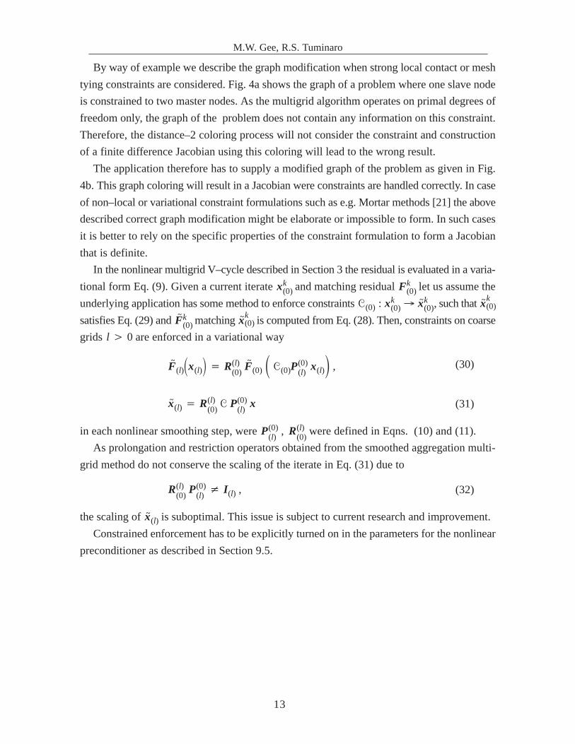
In the latter case of colored finite differencing for an approbiate Jacobian, a graph contain-

ing all potential Jacobian entries for constraints has to be supplied and is used in the coloring

and finite differencing process.

a) Wrong graph coloring as it would appear without additional constraint information

mesh–tying/contactconstraint

b) Correct graph coloring on constraint–modified graph

Figure 4: Distance–2 graph coloring of constraint–modified graph

It is requested by the implementation of the method through the getModifiedGraph()

method described in Section 9.2. The way in which the graph has to be modified depends on

the type of the constraints and is not prescribed by the solver.


13

By way of example we describe the graph modification when strong local contact or mesh

tying constraints are considered. Fig. 4a shows the graph of a problem where one slave node

is constrained to two master nodes. As the multigrid algorithm operates on primal degrees of

freedom only, the graph of the problem does not contain any information on this constraint.

Therefore, the distance–2 coloring process will not consider the constraint and construction

of a finite difference Jacobian using this coloring will lead to the wrong result.

The application therefore has to supply a modified graph of the problem as given in Fig.

4b. This graph coloring will result in a Jacobian were constraints are handled correctly. In case

of non–local or variational constraint formulations such as e.g. Mortar methods [21] the above

described correct graph modification might be elaborate or impossible to form. In such cases

it is better to rely on the specific properties of the constraint formulation to form a Jacobian

that is definite.

In the nonlinear multigrid V–cycle described in Section 3 the residual is evaluated in a varia-

tional form Eq. (9). Given a current iterate xk(0) and matching residual Fk

(0) let us assume the

underlying application has some method to enforce constraints �(0) : xk(0) � x~k

(0), such that x~k(0)

satisfies Eq. (29) and F~k

(0) matching x~k(0) is computed from Eq. (28). Then, constraints on coarse

grids l � 0 are enforced in a variational way

F~

(l)�x(l)�� R(l)(0)

F~

(0) � �(0)P(0)(l)

x(l)� , (30)

x~(l) � R(l)(0)

� P(0)(l)

x (31)

in each nonlinear smoothing step, were P(0)(l)

, R(l)(0)

were defined in Eqns. (10) and (11).

As prolongation and restriction operators obtained from the smoothed aggregation multi-

grid method do not conserve the scaling of the iterate in Eq. (31) due to

R(l)(0)

P(0)(l)

� I(l) , (32)

the scaling of x~(l) is suboptimal. This issue is subject to current research and improvement.

Constrained enforcement has to be explicitly turned on in the parameters for the nonlinear

preconditioner as described in Section 9.5.


14

8 Examples

8.1 One dimensional example

This simple example discretizes and solves

�2u�x2

� 103 u2� 0 , � � [0, 1] , u(x � 0) � 1 , u(x � 1) � 0 (33)

using linear finite elements. It is also provided as a user example with the distribution of

Trilinos/ML, see Section 9.6.

We fix the size of the generated coarsest grid to be 3000 equations and the coarsening rate

to be 1 : 3 for each level. This leads to an increase in the number of coarse grids as the problem

size is increased by refinement. We use colored finite differencing to obtain a fine grid Jacobian

matrix from which a smoothed aggregation multigrid hierachy is generated. We denote this set

of choices as ‘Version I’ in Fig. 5. As nonlinear smoothers, we select a polynomial smoother[1]

preconditioned nonlinear CG where the polynomial order is chosen as 4 on all grids. On the

coarsest grid, we use nonlinear CG preconditioned by a LU factorization of the variational coa-

resest level Jacobian. We apply a nonsymmetric V–cycle skipping all presmoothing steps on

all grids to avoid the presmoothing residual evaluations, applying 6 iterations on the coarsest

grid, 2 postsmoothing steps on every intermediate grid and 3 postsmoothing steps on the finest

grid, respectively. As convergence criteria, an absolute residual norm of 1.0e–07 is chosen.

1

10

100

1000

40000,00 400000,00 4000000,00

t [sec]

unknowns0

10

20

30

40

50

0 500000 1000000 1500000

iterations

unknowns

Version I: nonlinear MG Version II: linear MG

total

residual eval.

total

residual eval.

Figure 5: Solution times


15

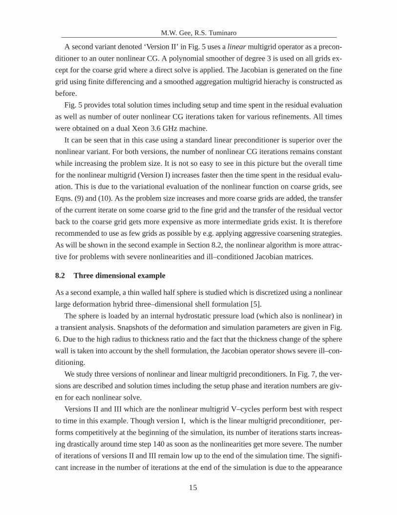
A second variant denoted ‘Version II’ in Fig. 5 uses a linear multigrid operator as a precon-

ditioner to an outer nonlinear CG. A polynomial smoother of degree 3 is used on all grids ex-

cept for the coarse grid where a direct solve is applied. The Jacobian is generated on the fine

grid using finite differencing and a smoothed aggregation multigrid hierachy is constructed as

before.

Fig. 5 provides total solution times including setup and time spent in the residual evaluation

as well as number of outer nonlinear CG iterations taken for various refinements. All times

were obtained on a dual Xeon 3.6 GHz machine.

It can be seen that in this case using a standard linear preconditioner is superior over the

nonlinear variant. For both versions, the number of nonlinear CG iterations remains constant

while increasing the problem size. It is not so easy to see in this picture but the overall time

for the nonlinear multigrid (Version I) increases faster then the time spent in the residual evalu-

ation. This is due to the variational evaluation of the nonlinear function on coarse grids, see

Eqns. (9) and (10). As the problem size increases and more coarse grids are added, the transfer

of the current iterate on some coarse grid to the fine grid and the transfer of the residual vector

back to the coarse grid gets more expensive as more intermediate grids exist. It is therefore

recommended to use as few grids as possible by e.g. applying aggressive coarsening strategies.

As will be shown in the second example in Section 8.2, the nonlinear algorithm is more attrac-

tive for problems with severe nonlinearities and ill–conditioned Jacobian matrices.

8.2 Three dimensional example

As a second example, a thin walled half sphere is studied which is discretized using a nonlinear

large deformation hybrid three–dimensional shell formulation [5].

The sphere is loaded by an internal hydrostatic pressure load (which also is nonlinear) in

a transient analysis. Snapshots of the deformation and simulation parameters are given in Fig.

6. Due to the high radius to thickness ratio and the fact that the thickness change of the sphere

wall is taken into account by the shell formulation, the Jacobian operator shows severe ill–con-

ditioning.

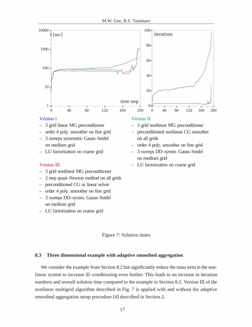
We study three versions of nonlinear and linear multigrid preconditioners. In Fig. 7, the ver-

sions are described and solution times including the setup phase and iteration numbers are giv-

en for each nonlinear solve.

Versions II and III which are the nonlinear multigrid V–cycles perform best with respect

to time in this example. Though version I, which is the linear multigrid preconditioner, per-

forms competitively at the beginning of the simulation, its number of iterations starts increas-

ing drastically around time step 140 as soon as the nonlinearities get more severe. The number

of iterations of versions II and III remain low up to the end of the simulation time. The signifi-

cant increase in the number of iterations at the end of the simulation is due to the appearance


16

of dynamic buckling of the structure which should make an adjustement of the time step size

necessary at that time.

t � 0 sec

– shell discretization includes thickness change of shell wall

– radius / thickness = 100 – Ogden hyperelastic material – hydrostatic internal pressure load – 19926 equations – implicit nonlinear dynamic analysis

(generalized–alpha–method)– 193 load steps, �t = 0.01 sec

t � 1 sec

t � 1.93 sec

Figure 6: Half sphere under hydrostatic pressure


17

Version I– 3 grid linear MG preconditioner– order 4 poly. smoother on fine grid– 3 sweeps symmetric Gauss–Seidel

on medium grid – LU factorization on coarse grid

Version III– 3 grid nonlinear MG preconditioner– 2 step quasi–Newton method on all grids– preconditioned CG as linear solver– order 4 poly. smoother on fine grid– 3 sweeps DD–symm. Gauss–Seidel


1

10

100

1000

10000

0 40 80 120 160 200

t [sec]

time step0

20

40

60

80

100

0 40 80 120 160 200

iterations

Version II– 3 grid nonlinear MG preconditioner– preconditioned nonlinear CG smoother

on all grids– order 4 poly. smoother on fine grid– 3 sweeps DD–symm. Gauss–Seidel


Figure 7: Solution times

8.3 Three dimensional example with adaptive smoothed aggregation

We consider the example from Section 8.2 but significantly reduce the mass term in the non-

linear system to increase ill–conditioning even further. This leads to an increase in iteration

numbers and overall solution time compared to the example in Section 8.2. Version III of the

nonlinear multigrid algorithm described in Fig. 7 is applied with and without the adaptive

smoothed aggregation setup procedure [4] described in Section 2.


18

– in clock–wise order: first, second and third near–nullspace mode

– 3 level adaptive multigrid setupusing symmetric Gauss–Seidel and 20 V–cycles on all levels to determine near–nullspace components

Figure 8: Near–nullspace modes from adaptive smoothed aggregation setup

An initial smoothed aggregation multigrid preconditioner is constructed based on the 6 rigid

body modes of the structure and the adaptive smoothed aggregation procedure is applied to

compute an additional 3 near–nullspace modes visualized in Fig. 8 that are not well–captured

by the existing multigrid preconditioner. The initial 6 rigid body modes together with 3 adat-

pively computed near–nullspace modes are then incorporated in a refined multigrid hierachy

which is then used in the nonlinear multigrid iteration described in Section 3.

Iteration numbers and solution times that include all setup costs are given in Fig. 9 for a

simulation applying 123 time steps.

In Fig. 9 the overall solution time benefits from the adaptive setup even though there is a

significantly higher setup cost for the adaptive multigrid hierachy in each time step and a

slightly increased cost for the application of one nonlinear V–cycle. The peak that can be seen

in Fig. 9 at time step 65 is due to geometric buckling phenomena which drives the determinant

of the Jacobian close to zero thus significantly increasing the condition number of the problem.

Remark 4: Efficieny can be increased even further if the once computed near–nullspace modesare resused in several consecutive solves as the setup procedure of the adaptive smoo-thed aggregation method contributes a major component to the overall solution time.This approach was not used here to demonstrate competitiveness of the adaptive me-thod in each individual solve.


19

It can also be expected that the benefit from the adaptive procedure is even higher in the

case of more complex models with e.g. jumps in material coefficients, where algebraically

smooth solution components are less well captured by the standard smoothed aggregation mul-

tigrid approach.

0

200

400

600

800

1000

1200

1400

0 40 80 120

t [sec]

time step0

10

20

30

0 40 80 120

iterations

adaptive SAadaptive SA

SASA

Figure 9: Solution times with adaptive smothed aggregation setup

9 Implementation documentation

9.1 Availability and configuration of Trilinos and ML

The proposed algorithm is part of the ML [15] package within the Trilinos [9] framework.

It is contained in the Trilinos developer version and in Trilinos 6.0 and later releases. Note that

this report refers to the Trilinos 6.0 version of the code.

––enable–ml ––with–ml_metis ––with–ml_nox

––enable–nox ––enable–nox–epetra ––enable–prerelease

––enable–epetra ––enable–epetraext

––enable–teuchos

––enable–aztecoo

––enable–amesos

––with–ldflags=”–L/<METIS_PATH>”

––with–incdirs=”–I/<METIS_PATH>/Lib”

––with–libs=”–lmetis”

Figure 10: Configuring Trilinos for use of nonlinear MG

As the method makes use of several of Trilinos’ subpackages such as ML, NOX, Epetra and

EpetraExt, Trilinos has to be configured such that all neccessary subpackages are present. To


20

do so, the configure options given in Fig. 10 should be included in the Trilinos configuration.

For general installation and usage instructions for Trilinos and ML, see [9] and [15].

In some choices of aggregation schemes, ML makes use of the third party library Metis [13]

not contained in the Trilinos distribution. The user has to provide the Metis library when con-

figuring and compiling Trilinos, see Fig. 10.

9.2 The application interface

The interface between an underlying nonlinear application and the nonlinear multigrid pre-

conditioner or solver is entirely contained in a virtual class called

ML_NOX::ML_Nox_Fineinterface contained in the file

Trilinos/packages/ml/src/NonlinML/ml_nox_fineinterface.H .

The user has to provide an implementation of this virtual class. Data from the solver such

as e.g. the current solution iterate will be passed to the underlying application through this in-

terface and the application has to provide information such as a residual vector or a graph of

the problem to the solver. The virtual class ML_NOX::ML_Nox_Fineinterface itself in-

herits from three different types of NOX’s interface classes.

Remark 5: It shall be stressed that all data passed to and from the solver through this interfacerefers to the finest grid which is the one the user is interested in solving. No data asso-ciated with any coarse grids nor a coarse grid interface need to be provided as datais passed to coarse grids through automatically generated coarse grid interfaces thatobtain data from the described fine grid interface. Most data is passed as Epetra distri-buted objects. Please refer to the Epetra user manual [11] for a detailed description.

In the following, a brief description of the methods in ML_NOX::ML_Nox_Fineinter-

face is given. Pure virtual methods have to be implemented by the user’s derived class.


21

virtual bool computeF( const Epetra_Vector& x, Epetra_Vector& FVec,

FillType flag) = 0;

The solver provides the current iterate (solution vector) in x and ex-pects the underlying application to reevaluate the residual vectorand store it in FVec.

virtual bool computeJacobian(const Epetra_Vector& x) = 0;

The solver provides the current iterate (solution vector) in x and ex-pects the application to reevaluate the Jacobian matrix and store itso it can be accessed by the method getJacobian() described be-low. This method will only be used in cases where the user specifiedusage of an application provided Jacobian in the input options, seeSection 9.5.

virtual Epetra_CrsMatrix* getJacobian() = 0;

The method returns a pointer to the Jacobian evaluated at the mostrecent call to computeJacobian() described above. This methodwill only be used in cases where the user specified usage of an ap-plication provided Jacobian in the input options.

virtual bool computePreconditioner(const Epetra_Vector& x) = 0;

The method is currently not used by the algorithm. It has to be im-plemented though (e.g. with an error message) as it is derived froman underlying NOX virtual class.

virtual const Epetra_CrsGraph* getGraph() = 0;

The method returns the graph of the problem. This could either bethe graph underlying the Jacobian matrix if present or, in the casethe application does not provide a Jacobian, it has to be a graphinstance computed and stored for this purpose by the underlying ap-plication.

virtual const Epetra_CrsGraph* getModifiedGraph() = 0;

The method returns the modified graph of the constrained problemas described in Section 7.


22

virtual const Epetra_Map& getMap() = 0;

The method returns the Epetra map associated with the solutionvector. It is crucial that this map is pointwise identical to the map ofthe residual vector, the pointwise row map of the Jacobian and thepointwise row map of the supplied graph. In parallel, any map mightbe specified though the performance of the algorithm benefits fromwell chosen distributions of the unknowns as can be generated usinga partitioning library such as e.g. Metis [13].

virtual double* Get_Nullspace( const int nummyrows, const int numpde,

const int dim_nullsp) = 0;

The method returns vectors representing an approximation to thenullspace of the nonlinear PDE operator. In case of elasticity prob-lems, these vectors contain the six rigid body modes of the discretedomain on the fine grid. The rigid body modes can be easily com-puted using nodal coordinates of the fine discretization, for detailssee [15] and the example in Fig. 11. They are used in the construc-tion of the algebraic prolongation and restriction operators and playa crucial role to the performance of the overall algorithm. The pa-rameters provided are:nummyrows Number of local rows of a nullspace vector on a

processnumpde Maximum number of degrees of freedom per

node as specified in the solver options by the user.dim_nullsp Number of nullspace vectors expected by the

solver. If the user specified the dimension of theproblem as ‘3’ on input, the algorithm expects sixvectors, if the dimension of the problem was specified as ‘2’ or as ‘1’, the algorithm expects three or one nullspace vector, respectively.

If the method returns NULL, ML’s default nullspace will be usedwhich might lead to slower convergence rates.

virtual const Epetra_Vector* getSolution() = 0;

The method returns the initial guess or the latest solution iteratestored by the application. It is used only in cases where the nonlinearmultigrid is used as a standalone solver instead of as a precondition-er. If a preconditioner is used, implementing an error message is suf-ficient.


23

rigid body modes::

translation in x

rotation round x

noda

l deg

rees

of fr

eedo

mx–direction

y–direction

z–direction

translation in y

translation in z

rotation round y

rotation round z

1

0

0

0

1

0

0

0

1

0

x^ 3�x3

x2�x^ 2

x3�x^ 3

0

x^ 1�x1

x^ 2�x2

x1�x^ 1

0

x : nodal coordinates

x^ : coordinates of an arbitrary reference point

Figure 11: Nullspace for continuum discretization

virtual bool Get_BlockInfo( int* nblocks, int** blocks,

int** block_pde) = 0;

The method is used if the ‘VBMETIS’ aggregation scheme is cho-sen by the user on input, see Section 9.5. This aggregation schemeprovides support for variable blocked problems when the numberof degrees of freedom per node is non–constant throughout the sys-tem of equations. In this case the user has to provide additional in-formation about the nodal block structure of the problem.nblocks (output) Local number of blocks on a processblocks (output) Allocated vector of local length match–

ing the row map obtained by getMap(). Contains global numbering of blocks where the index base is zero.

block_pde (output) Allocated vector of local length match–ing the row map obtained by getMap(). Contains the number of the PDE equation each

point row entry belongs to, where the index base is zero.Both allocated vectors are destroyed by the solver when no longerneeded. If the method returns false on exit, the aggregationscheme ‘METIS’ is used and a constant block size is assumed. Anexample for the construction of this block information is given inFig. 12.


24

node 0

X X X

X X X

X X X

X X X

X X X

X X X

X

X

X

X X X X

X

X

X

X

X X

X X

X X

X X X

X X X

node 1

node 2

blocks

block_pde

*nblocks = 3

0 0 0 1 1 1 1 2 2

0 1 2 0 1 2 3 0 1

graph:

block data:

Figure 12: Variable block data

bool isnewJacobian() { return isnewJacobian_; }

Returns the variable bool isnewJacobian_ from class ML_NOX::ML_Nox_Fineinterface. This variable shouldbe set to true by computeJacobian whenever a Jacobian is re-evaluated. It should be set to false by computeF whenever anew residual is evaluated. This allows the solver to determinewhether the current Jacobian matches the current residual.

int getnumJacobian() { return numJacobian_; }

Returns the variable int numJacobian_ from class ML_NOX::ML_Nox_Fineinterface. This variable shouldbe incremented by computeJacobian whenever a Jacobian isreevaluated. It is used for statistical output.

void resetsumtime() { t_ = 0.; return; }

Used internally to reset the summed time spent in the interface. Itis used to measure time spent in the interface and application sepa-rately for the solver setup and the iteration phase. It is used for statis-tical output.


25

int getnumcallscomputeF() { return ncalls_computeF_ }

Returns the variable int ncalls_computeF_ from class ML_NOX::ML_Nox_Fineinterface. This variable shouldbe incremented by computeF whenever a residual is reevaluated.It is used for statistical output.

bool setnumcallscomputeF(int ncalls) { ncalls_computeF_=ncalls;

return true;}

Used internally to reset the variable int ncalls_computeF_

from class ML_NOX::ML_Nox_Fineinterface. It is usedto measure the number of calls to computeF separately for thesetup phase and in the total.

9.3 Nonlinear multigrid as a solver

The nonlinear multigrid class can be used as a solver though in most cases it is recommended

to use it as a preconditioner to some outer nonlinear iteration, see Section 9.4. Here we describe

the principal setup of the method in Fig. 13 using the solver capability of the class.

The nonlinear multigrid class can be constructed (Fig. 13, line 108) after defining an ��

�� derived communicator object, a map reflecting the distribution of solution and re-

sidual vectors, rows of the problem graph and the Jacobian. Detailed function documentation

is also provided in the Trilinos/packages/ml/doc directory of the distribution. Fol-

lowing line 110 in Fig. 13, a variety of options can be chosen which are discussed in detail in

Section 9.5.

After all options are chosen and passed to the ML_NOX::ML_Nox_Preconditioner

class, the solve() method starts the setup phase and the iterative solution procedure of the

multigrid method.

9.4 Nonlinear multigrid as a preconditioner

It is recommended to use the nonlinear multigrid as a preconditioner to some outer nonlinear

Krylov iteration. The basic setup of the preconditioner has already been described in Section

9.3. Additionally, the user has to setup the outer Krylov solver and register the preconditioner

with it. As describing the setup of a NOX solver would exceed the purpose of this report, we

refer to [16] and the example application provided with the distribution and described in Sec-

tion 9.6.


26

0 #ifdef PARALLEL

1 #include “Epetra_MpiComm.h”

2 #else

3 #include “Epetra_SerialComm.h”

4 #endif

5

6 #include “Epetra_Map.h”

7

8 #include “myinterface.H“

9 #include “ml_nox_preconditioner.H”

(...)

50 #ifdef PARALLEL

51 Epetra_MpiComm Comm(mpicomm);

52 #else

53 Epetra_SerialComm Comm();

54 #endif

(...)

100 // create the ML_NOX::ML_Nox_Fineinterface

101 // derived application interface

102 MY_APP_INTERFACE inter(Comm);

103

104 // get the fine grid row– and vector map

105 Epetra_Map& map = inter.GetMap();

106

107 // create the nonlinear multigrid class

108 ML_NOX::ML_Nox_Preconditioner Prec(inter,map,map,Comm);

109

110 // choose options

(...)

150 // solve

151 bool ok = Prec.solve();

Figure 13: Setup of the nonlinear algorithm

9.5 Nonlinear preconditioner options

Once the ML_NOX::ML_Nox_Preconditioner class is created as shown in Fig. 13, line

108, there exist several methods to pass options to the class and override the default configura-

tion.

In the following, options as well as the methods to pass options to the preconditioner class are

listed and discussed. Note that some option choices might conflict or might not have any effect

at all depending on how other parameters are chosen. It is therefore recommended to study the

variants carefully.


27

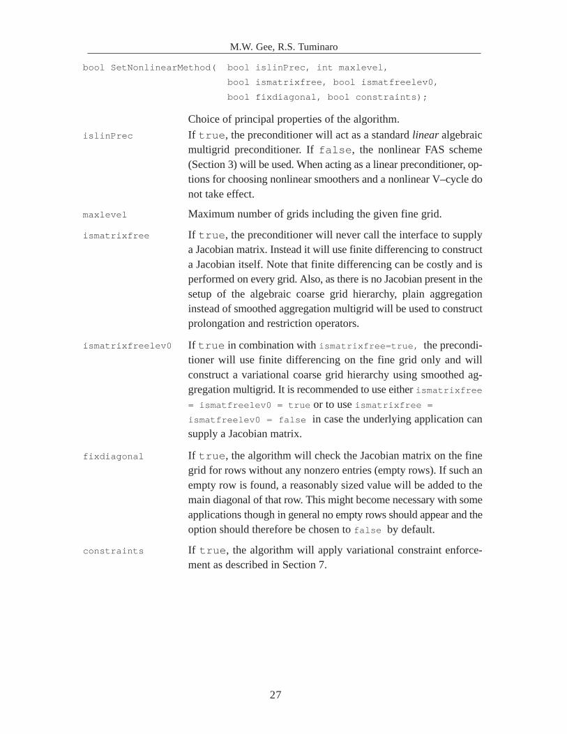
bool SetNonlinearMethod( bool islinPrec, int maxlevel,

bool ismatrixfree, bool ismatfreelev0,

bool fixdiagonal, bool constraints);

Choice of principal properties of the algorithm.

islinPrec If true, the preconditioner will act as a standard linear algebraicmultigrid preconditioner. If false, the nonlinear FAS scheme(Section 3) will be used. When acting as a linear preconditioner, op-tions for choosing nonlinear smoothers and a nonlinear V–cycle donot take effect.

maxlevel Maximum number of grids including the given fine grid.

ismatrixfree If true, the preconditioner will never call the interface to supplya Jacobian matrix. Instead it will use finite differencing to constructa Jacobian itself. Note that finite differencing can be costly and isperformed on every grid. Also, as there is no Jacobian present in thesetup of the algebraic coarse grid hierarchy, plain aggregationinstead of smoothed aggregation multigrid will be used to constructprolongation and restriction operators.

ismatrixfreelev0 If true in combination with ismatrixfree=true, the precondi-tioner will use finite differencing on the fine grid only and willconstruct a variational coarse grid hierarchy using smoothed ag-gregation multigrid. It is recommended to use either ismatrixfree

= ismatfreelev0 = true or to use ismatrixfree = ismatfreelev0 = false in case the underlying application cansupply a Jacobian matrix.

fixdiagonal If true, the algorithm will check the Jacobian matrix on the finegrid for rows without any nonzero entries (empty rows). If such anempty row is found, a reasonably sized value will be added to themain diagonal of that row. This might become necessary with someapplications though in general no empty rows should appear and theoption should therefore be chosen to false by default.

constraints If true, the algorithm will apply variational constraint enforce-ment as described in Section 7.


28

bool SetNonlinearSolvers( bool usenlnCG_fine, bool usenlnCG,

bool usenlnCG_coarse, bool useBroyden,

int niters_fine, int niters,

int niters_coarse);

Choice of nonlinear smoothing and solving algorithm and the maxi-mum number of iterations to be taken on distinct grids.

usenlnCG_fine,

usenlnCG,

usenlnCG_coarse

If true, the preconditioner will use nonlinear CG as a nonlinearmethod on the fine, all intermediate and on the coarse grid, respec-tively. If false, quasi–Newton method will be used. Usage of non-linear CG and Newton’s method can be mixed among grids.

niters_fine,

niters,

niters_coarse

When choosing a quasi–Newton method on a grid, a linear CG solvewill be performed inside each Newton step. The maximum numberof linear CG iterations to be taken can be specified by these vari-ables. These options do not take effect when nonlinear CG is chosenas the nonlinear smoothing method.

bool SetPrintLevel(int ml_printlevel);

Choice of the amount of output to be generated during setup and it-eration. ml_printlevel can take values between 0 (no output) and10 (full output). A value of 6 results in a reasonable amount of infor-mation.

bool SetDimensions( int spatialDimension, int numPDE, int dimNS);

Provide information about the spatial dimension of the problem, thenodal block size and the nullspace to be used.

spatialDimension Specify 1, 2 or 3 for 1D, 2D or 3D problems, respectively.

numPDE Number of PDE equations. In general equal to the number of de-grees of freedom per node on the fine grid and the nodal block sizeof the Jacobian matrix. If the aggregation scheme “VBMETIS” isused and the problem is of variable block size, the largest block sizein the system has to be specified.

dimNS Dimension of the approximation to the nullspace of the fine gridnonlinear operator, see Section 2. For 3D structural problems, thisusually would be the 6 rigid body modes of the discretized body ne-glecting Dirichlet boundary conditions. The number of nullspacevectors dimNS has to be larger or equal to numPDE.


29

bool SetCoarsenType( string coarsentype, int maxlevel,

int maxcoarsesize, int nnodeperagg);

Choice of ML’s aggregation method in the generation of the coarsegrid hierachy.

coarsentype Though ML supports several other aggregation schemes, the nonlin-ear preconditioner class currently supports “Uncoupled”, “ME-TIS” and “VBMETIS”, see also [15]. The “VBMETIS” schemeis currently the only scheme supporting problems with nonconstantnodal blocks, also see Sections 2 and 9.2. “VBMETIS” can also beused for constant block sized problems though the “METIS”scheme is more efficient in this case resulting in an identical gridhierarchy.

maxlevel Maximum number of levels to be generated. The maximum numberof levels to be used depends on the problem size but should be keptas small as possible without resulting in a too large coarse grid prob-lem.

maxcoarsesize The setup of the multigrid hierachy stops generating coarser gridswhen the current coarsest grid has less than maxcoarsesize equa-tions.

nnodeperagg When using the “METIS” or “VBMETIS” aggregation scheme,the target number of nodal blocks per aggregate can be specified.Standard choices are 9 in 2D and 27 in 3D. Choosing less nodes peraggregate results in larger and eventually more coarse grids, choos-ing more nodes per aggregate results in a faster decay of grid sizeand eventually less coarse grids (a ‘cheaper’ coarse grid hierarchy)at the cost of reduced convergence rates. The option does not haveany effect when the “Uncoupled” aggregation scheme is chosen.

bool SetConvergenceCriteria( double FAS_normF, double FAS_nupdate);

Choose the convergence criteria norm of the residual vector andnorm of the update vector for all grids. The nonlinear smoothing it-eration (nonlinear CG or quasi–Newton method) on a grid will ter-minate successfully when either of these criteria is met. Note thatthese criteria should be chosen equal or smaller than for the outsidenonlinear Krylov method if used as a preconditioner.


30

bool SetRecomputeOffset( int offset );

bool SetRecomputeOffset( int offset, int recomputestep,

double adaptrecompute, int adaptns);

Options to choose when to recompute the multigrid hierachy. Oncethe multigrid hierachy and the Jacobian operators are computedthey do not change throughout the nonlinear iteration. In order tospeed up the iteration process it might be useful to recompute thisdata from time to time. Several ways to do so can be chosen usingthese parameters.

offset Every offset nonlinear iterations, the multigrid hierachy and Ja-cobian operators are destroyed and recomputed from scratch. If norecomputation is desired, offset should be chosen as a very largenumber.

recomputestep It might be advantagous to recompute the multigid hierachy onceafter a few nonlinear iterations have taken place. When comingcloser to the solution, the approximation quality of the Jacobian op-erators and the multigrid preconditioner increases. The multigridhierarchy is recomputed once after the recomputestep iteration.Choosing recomputestep to 0 indicates that the hierarchy is notrecomputed.

adaptrecompute If the initial guess to the nonlinear iteration is far from the solution,the nonlinear multigrid preconditioner might have poor approxima-tion properties and divergence might occur. The multigrid hierachyis recomputed every time the residual norm of the outside Krylovmethod is larger than adaptrecompute. Choosing adaptrecom-pute to 0.0 will not recompute the hierachy.

adaptns Number of additional near–nullspace components to be computedby an adaptive smoothed aggregation setup procedure, see also Sec-tions 2, 8.3 and [4]. If chosen to 0, no adaptive setup will be per-formed.


31

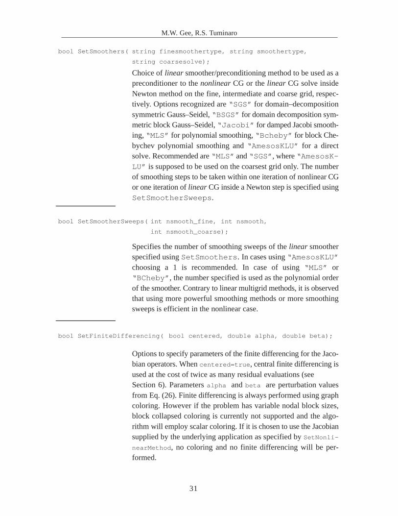
bool SetSmoothers( string finesmoothertype, string smoothertype,

string coarsesolve);

Choice of linear smoother/preconditioning method to be used as apreconditioner to the nonlinear CG or the linear CG solve insideNewton method on the fine, intermediate and coarse grid, respec-tively. Options recognized are “SGS” for domain–decompositionsymmetric Gauss–Seidel, “BSGS” for domain decomposition sym-metric block Gauss–Seidel, “Jacobi” for damped Jacobi smooth-ing, “MLS” for polynomial smoothing, “Bcheby” for block Che-bychev polynomial smoothing and “AmesosKLU” for a directsolve. Recommended are “MLS” and “SGS”, where “AmesosK-LU” is supposed to be used on the coarsest grid only. The numberof smoothing steps to be taken within one iteration of nonlinear CGor one iteration of linear CG inside a Newton step is specified usingSetSmootherSweeps.

bool SetSmootherSweeps( int nsmooth_fine, int nsmooth,

int nsmooth_coarse);

Specifies the number of smoothing sweeps of the linear smootherspecified using SetSmoothers� In cases using “AmesosKLU”choosing a 1 is recommended. In case of using “MLS” or“BCheby”, the number specified is used as the polynomial orderof the smoother. Contrary to linear multigrid methods, it is observedthat using more powerful smoothing methods or more smoothingsweeps is efficient in the nonlinear case.

bool SetFiniteDifferencing( bool centered, double alpha, double beta);

Options to specify parameters of the finite differencing for the Jaco-bian operators. When centered=true, central finite differencing isused at the cost of twice as many residual evaluations (see Section 6). Parameters alpha and beta are perturbation valuesfrom Eq. (26). Finite differencing is always performed using graphcoloring. However if the problem has variable nodal block sizes,block collapsed coloring is currently not supported and the algo-rithm will employ scalar coloring. If it is chosen to use the Jacobiansupplied by the underlying application as specified by SetNonli-

nearMethod, no coloring and no finite differencing will be per-formed.


32

bool SetFAScycle( int prefsmooth, int presmooth,

int coarsesmooth, int postsmooth,

int postfsmooth, int maxcycle);

Options to specify the layout of the potentially nonsymmetric FAS V–cycle. For the finest,intermediate and coarsest grids, the maximum number of presmoothing, coarse grid andpostsmoothing iterations can be chosen. Choosing pre– and post iteration numbers different-ly results in a nonsymmetric V–cycle. Except for coarsesmooth, all values can also be inde-pendently chosen to be zero, see also Fig. 14a.When convergence is achieved on some intermediate grid in the presmoothing phase, nocoarser grid is visited but instead the algorithm returns to the postsmoothing phase of thenext finer grid. For a graphical illustration, see Fig. 14b.

outer nonlinear CG

fine

coarse

prefsmooth=0

presmooth=2

presmooth=2

presmooth=2

coarsesmooth=4

postfsmooth=4

postsmooth=3

postsmooth=3

postsmooth=3

outer nonlinear CG

convergence criteria is met

proceed to postsmoothing on next finer grid

a) nonsymmetric FAS V–cycle, options for pre– and postsmoothing number of iterations

b) convergence during presmoothing step

Figure 14: Nonsymmetric FAS v–cycle


33

9.6 Example application

An example application using the nonlinear multigrid is given in the subdirectory

Trilinos/packages/ml/examples/NonlinML/

of the Trilinos installation. It is a simple one dimensional nonlinear finite element problem

where the number of elements is specified by the user on the command line. A sufficiently large

number (e.g. 10000) must be specified to allow for generation of at least one coarse grid by

ML.

The file ml_nox_1Delasticity_example.cpp contains the main routine

where all solver parameters are set. The files FiniteElementProblem.cpp and Prob-

lem_Interface.cpp contain the underlying application and the interface between ap-

plication and solver, respectively. The latter is a good example on how the interface described

in Section 9.2 is implemented while the main routine contains one choice of solver options de-

scribed in Section 9.5.

10 Conclusion

A nonlinear multigrid solver is described. This description includes algorithm basics as well

as detailed user instructions for setting up and directing the solver. More information can be

found within ML’s documentation and example directories.

11 References

[1] Adams, M., Brezina, M., Hu, J., Tuminaro, R. (2003): Parallel multigrid smoothing:

Polynomial versus Gauss–Seidel. J. Comp. Physics, 188/2, 593–610.

[2] Al–Baali, M., Fletcher, R. (1996): On the order of convergence of preconditioned non-

linear conjugate gradient methods. SIAM J. Sci. Comput., 17, 658–665.

[3] Brandt, A. (1977): Multi–Level Adaptive Solutions to Boundary Value Problems. Math.

Comp., 31, 333–390.

[4] Brezina, M., Falgout, R., MacLachlan, S., Manteuffel, T., McCormick, S., Ruge, J.

(2004): Adaptive Smoothed Aggregation (�SA). SIAM J. Sci. Comp., 25, 1896–1920.

[5] Büchter, N., Ramm, E., Roehl, D. (1994): Three Dimensional Extension of Nonlinear

Shell Formulation Based on the Enhanced Assumed Strain Concept. Int. J. Num. Meth.

Eng., 37, 2551–2568.

[6] Briggs, W.L., Henson, V.E., McCormick, S.F. (2000): A Multigrid Tutorial, Second

Edition. SIAM Press.


34

[7] Fletcher, R. (1987): Practical Methods of Optimization, Second Ed.. Wiley, Chichester,

England.

[8] Heinstein, M.W., Key, S.W., Blanford, M.L. (): A Multigrid Method for Matrix–free

Solutions of Non–Linear Quasistatic FE Solid Mechanics Problems. Draft, Sandia Na-

tional Laboratories.

[9] Heroux, M. Allen, M., Sala, M. (2004): An Overview of the Trilinos package. Technical

Report No. SAND2004–1949C, Sandia National Laboratories.

[10] Heroux, M. (2005): AztecOO User Guide. Technical Report No. SAND2004–3796, San-

dia National Laboratories. software.sandia.gov/trilinos/packages/aztecoo .

[11] Heroux, M., Hoekstra, R.J., Williams, A. (2005): Epetra User Guide. Technical Report

No. SAND2004–xxxx, Sandia National Laboratories. software.sandia.gov/packages/

epetra .

[12] Hoekstra, R., Cross, J., Heroux, M., Willenbring, J., Williams, A. (2005): EpetraExt

linear algebra package. software.sandia.gov/packages/epetraext .

[13] Karypis, G., Kumar, V. (1998): METIS 4.0: Unstructured graph partitioning and sparse

matrix ordering system. technical report, Deprtment of Computer Science, Univ. of Mi-

nessota.

[14] Kelley, C.T. (2003): Solving Nonlinear Equations with Newton’s Method. in ‘Fundamen-

tals of Algorithms’ series, SIAM Press.

[15] Sala, M., Tuminaro, R.S., Hu, J.J., Gee, M.W. (2005): ML 4.0 Smoothed Aggregation

User’s Guide. Technical Report No. SAND2004–4819, Sandia National Laboratories.

software.sandia.gov/trilinos/packages/ml .

[16] Kolda, T., Pawolwski, R., Bader, B., Hooper, R., Phipps, E., Salinger, A. (2005): NOX/

LOCA nonlinear solvers and path following algorithms package within Trilinos. soft-

ware.sandia.gov/nox .

[17] Shewchuk, J.R. (1994): An Introdution to the Conjugate Gradient Method Without the

Agonizing Pain. Technical Report, Carnegie Mellon Univ. .

[18] Vanek, P., Mandel, J., Brezina, M. (1996): Algebraic Multigrid by Smoothed Aggrega-

tion for Second and Fourth Order Elliptic Problems, Computing, 56, 179–196.

[19] Vanek, P., Brezina, M., Tezaur, R. (1999): Two–Grid Method for Linear Elasticity on

Unstructured Meshes, SIAM Journal on Scientific Computing, 21, 900–923.


35

[20] Vanek, P., Brezina, M., Mandel, J. (2001): Convergence of algebraic multigrid based

on smoothed aggregation, Numerische Mathematik, 88, 559–579.

[21] Wohlmuth, B.I. (2001): Discretization Methods and Iterative Solvers Based on Domain

Decomposition. Lecture Notes in Computational Science and Engineering 17, Springer

Press, Berlin, Germany.

nonlinear algebraic multigrid for constrained solid ... · sand2006–2256 unlimited release...

Documents