nonlinear analysis of layered structures with weak … · laboratoire de mécanique et milieux...
TRANSCRIPT

POUR L'OBTENTION DU GRADE DE DOCTEUR ÈS SCIENCES
PAR
M.Sc. in Mechanics and Machine Design, Cracow University of Technology, Cracow, Pologneet de nationalité polonaise
acceptée sur proposition du jury:
Lausanne, EPFL2006
Prof. C. Ancey, président du juryProf. F. Frey, Prof. A. Zielinski, directeurs de thèse
Dr T. Kurtyka, rapporteurProf. J.-M. Reynouard, rapporteur
Prof. Y. Weinand, rapporteur
nonlinear analysis of layered structureswith weak interfaces
Piotr KRAWCZYK
THÈSE NO 3554 (2006)
ÉCOLE POLYTECHNIQUE FÉDÉRALE DE LAUSANNE
PRÉSENTÉE LE 22 JUIN 2006
à LA FACULTÉ ENVIRONNEMENT NATUREL, ARCHITECTURAL ET CONSTRUIT
Laboratoire de mécanique et milieux continus
SECTION DE GÉNIE CIVIL


There is nothing so practical as a good theory Kurt Lewin
To my parents


Contents: Summary .................................................................................................................................1 Résumé....................................................................................................................................2 Acknowledgments...................................................................................................................3 1. Introduction.....................................................................................................................4 2. Beams..............................................................................................................................6
2.1. Theoretical development.........................................................................................6 2.1.1. Kinematic relations .........................................................................................6 2.1.2. Geometric relations .......................................................................................10 2.1.3. Constitutive relations ....................................................................................12 2.1.4. Equilibrium relations.....................................................................................16
2.2. Finite element development ..................................................................................19 2.2.1. Co-rotational finite element formulation ......................................................19 2.2.2. Criteria for establishment of element interpolation ......................................23 2.2.3. Management of numerical locking ...............................................................24 2.2.4. Deforming displacement field evaluation .....................................................25 2.2.5. Management of layer-wise boundary conditions ..........................................27 2.2.6. Transverse refinement of shear stress ...........................................................28 2.2.7. Survey of investigated elements ...................................................................29
2.3. Numerical benchmarks .........................................................................................31 2.3.1. Patch tests......................................................................................................31 2.3.2. Cantilever bent by transverse force...............................................................32 2.3.3. Pagano test ....................................................................................................34 2.3.4. Ren test..........................................................................................................36 2.3.5. Buckling of laminated columns ....................................................................38 2.3.6. Beam-column with partial interaction...........................................................40 2.3.7. Uniform bending of cantilever ......................................................................42 2.3.8. Nonlinear buckling of sheathed walls ...........................................................44 2.3.9. Nonlinear response of hyperstatic laminated beam ......................................46 2.3.10. Steel-concrete bridge deck ............................................................................47
2.4. Summary for beam formulation............................................................................51 3. Plates .............................................................................................................................53
3.1. Theoretical development.......................................................................................53 3.1.1. Kinematic relations .......................................................................................53 3.1.2. Geometric relations .......................................................................................55 3.1.3. Constitutive relations ....................................................................................56 3.1.4. Equilibrium relations.....................................................................................57
3.2. Finite element development ..................................................................................60 3.2.1. Total-Lagrangian finite element formulation................................................60 3.2.2. Element topology and mapping ....................................................................62 3.2.3. Rotation of element vectors and matrices .....................................................63 3.2.4. Management of numerical locking ...............................................................64
3.3. Numerical benchmarks .........................................................................................68 3.3.1. Patch tests......................................................................................................68 3.3.2. Pagano test ....................................................................................................71 3.3.3. Uniform bending test ....................................................................................74 3.3.4. Nonlinear behaviour of laminated glass plates .............................................74 3.3.5. Laminated glass buckling..............................................................................76
3.4. Summary for plate formulation.............................................................................78 4. Shallow shells ...............................................................................................................79
4.1. Theoretical development.......................................................................................79

4.1.1. Kinematic relations .......................................................................................79 4.1.2. Geometric relations .......................................................................................83 4.1.3. Constitutive relations ....................................................................................84 4.1.4. Equilibrium relations.....................................................................................84
4.2. Finite element development ..................................................................................86 4.2.1. Co-rotational finite element formulation ......................................................86 4.2.2. On finite element implementation.................................................................87
4.3. Summary for shallow shell formulation................................................................88 5. Concluding remarks ......................................................................................................89 6. References .....................................................................................................................90 Curriculum Vitae...................................................................................................................95

- 1 -
Summary This work addresses nonlinear finite element analysis of laminated structures with weak interfaces. Considered first are shallow laminated beams subject to arbitrary large displacements, small layer strains and moderate interface slippage. Under these requirements rigorous development of layer-wise kinematic field is performed assuming First order Shear Deformation Theory (FSDT) at the layer level. The final form of this field is highly nonlinear and thus awkward in direct finite element (FE) implementation. However, the small strain assumption allows decomposition of element displacements into large rigid-body-motion and small deforming displacement field. In this case, the conjunction of linearized kinematic relations and the von Kármán strain measure applied in moving element frame allows for robust co-rotational FE formulation. This formulation is here extended to account for material nonlinear behaviour of layers and interfaces. To complete the development, means of obtaining efficient FE implementation are indicated. Discussed topics include the choice of suitable element interpolation schemes, proficient methods of alleviating numerical locking, evaluation of element deforming displacement field and management of layer-wise boundary conditions. In addition, a novel approach is proposed for a posteriori enhancement of the transverse shear stress distribution. Finally, the proposed model is tested with a number of demanding benchmark tests. The above modelling approach is next extended to geometric nonlinear analysis of laminated plates. Constraining plate displacements to be moderate (in von Kármán’s sense) and using Total-Lagrangian FE formulation it is shown that the simplicity and robustness of the beam formulation can be preserved also in plate analysis. FE solutions obtained with the adopted approach are again shown to provide reliable results in global and local scale. However, it is also indicated that methods used to alleviate shear locking in single-layer plate elements are not entirely satisfactory in multi-layer ones. Thus, FE implementation allowing for non-regular meshes needs yet to be identified. Considered next is the possibility of extending the developed plate model to the co-rotational FE analysis of shallow laminated shells. Primary concern here is assuring consistency of 3D rotations of element vectors and matrices. This problem is resolved here by modifying the description of interface displacement field and including vertex rotations in finite element kinematics. With these enhancements FE matrix formulation is constructed to allow geometric nonlinear analysis of shallow laminated shells subject to arbitrary large displacements, small layer strains and moderate interface slippage. Keywords: Laminated Structures, Layer-Wise Approach, Inter-Layer Slip, Large Displacements, Co-rotational Finite Element Formulation, Material Nonlinearity

- 2 -
Résumé Ce travail a pour cadre l’analyse non linéaire par éléments finis de structures multicouches avec glissement d’interface. Dans un premier temps, sont traitées les poutres multicouches, droites ou faiblement courbes, soumises à de grands déplacements produisant de petites dilatations dans les couches et à des glissements modérés aux interfaces. Sous ces conditions, une description rigoureuse de la cinématique des couches est effectuée sur la base de la théorie du premier ordre de la déformation à l’effort tranchant (FSDT) au niveau de chaque couche. La forme finale de cette cinématique est hautement non linéaire et est ainsi particulièrement embarrassante pour son introduction directe dans la formulation des éléments finis. Cependant, l’hypothèse des petites déformations autorise la décomposition du mouvement d’un élément en un champ de grands déplacements rigides et un champ de petits déplacements déformants. Dans ce cas, la conjonction de la linéarisation des relations cinématiques et de l’utilisation de la déformation de von Kármán, écrites dans le repère qui suit le mouvement de l’élément, permet d’obtenir une formulation corotationnelle robuste. Cette formulation est étendue au comportement non linéaire matériel des couches et des interfaces. Pour compléter ces développements, on indique les moyens d’obtenir une implémentation efficace des éléments finis. En particulier, les sujets suivants sont discutés : le choix des schémas adéquats d’interpolation des éléments, les méthodes efficaces pour éviter les divers verrouillages numériques, la manière d’évaluer les déplacements déformants de l’élément et la gestion des conditions de bord. De plus, une nouvelle approche est proposée pour l’enrichissement a posteriori de la distribution des contraintes de cisaillement transverse. Finalement, le modèle proposé est vérifié à l’aide de plusieurs benchmarks exigeants. La même approche de modélisation est étendue ensuite à l’analyse géométriquement non linéaire des plaques multicouches. En se restreignant aux déplacements modérés (au sens de von Kármán) et en utilisant la formulation lagrangienne totale, on montre que la simplicité et la robustesse de la formulation développée pour les poutres peuvent être conservées pour l’analyse des plaques multicouches. Les solutions obtenues par cette approche fournissent également des valeurs sûres tant dans le comportement global que local. Par contre, il est mis en évidence que les méthodes utilisées pour éviter le verrouillage d’effort tranchant pour les plaques à une seule couche ne donnent pas entière satisfaction dans le cas des plaques multicouches. Ainsi, une autre approche par rapport à ce problème doit être identifiée pour les réseaux non réguliers. On considère ensuite la possibilité d’étendre le modèle de plaque développé à l’analyse en formulation corotationnelle des coques légèrement courbes. La première exigence est d’assurer la consistance des vecteurs et matrices en rotation tridimensionnelle. Cette question est résolue ici en modifiant la description du champ des déplacements aux interfaces et en incluant les rotations "vertex" dans la cinématique de chaque couche. Avec cet apport, la formulation proposée permet l’analyse non linéaire géométrique des coques multicouches légèrement courbes soumises à de grands déplacements arbitraires induisant des petites déformations et des glissements modérés. Mots-clés: Structures Multicouches, Approche "Layer-Wise", Glissement d’interface, Grands Déplacements, Formulation Corotationnelle, Non Linéaire Matérielle.

- 3 -
Acknowledgments I would like to express my deepest gratitude to Prof. François Frey and Prof. Andrzej Zieliński for providing me the opportunity to work on this project and their kind support. I thank Blaise Rébora for his invaluable guidance, commitment and all the stimulating discussions we had. I am grateful to Prof. Adnan Ibrahimbegović for his contribution to this research. I would also like to thank all present and former collaborators at the LSC: Raphaël Bonnaz, Stéphane Bordas, Peter Grassl, Céline Neyroud, Nhi Nguyen, Matthias Preissig, Simon Rolshoven, Ann Schumacher, Birgitte Seem, Marc-André Studer and Thomas Zimmermann. Thank you for making LSC a niece and friendly place.
NONLINEAR ANALYSIS OF LAYERED STRUCTURES WITH WEAK INTERFACES
- 4 -
1. Introduction Basic theoretical provisions in the analysis of laminated structures emerge from the equilibrium of inter-laminar forces and are often referred to as the 0
zC -requirements [1], [2]. They can be summarized in the form of limitations imposed on transverse continuity of the stress and the strain fields at an interface of two layers with different thermo-mechanical properties. In such case, transverse stresses are required to maintain 0C continuity, whereas membrane stresses and the strain field may in general be discontinuous. This implicates that the transverse continuity of the displacement field at such interface cannot be imposed beyond the 0C level. Moreover, if complete layer interaction is not assured, the displacement field may also be discontinuous. As the traditional structural models are not capable of fulfilling the aforementioned limitations, new modelling approaches are being developed for analysis of laminated structures. Particularly investigated are theories a priori postulating certain kinematic field distribution in structure transverse direction. According to Reddy’s classification [1], these theories can be sub-divided into two major categories: the Equivalent-Single-Layer (ESL) and the Layer-Wise (LW) ones. ESL theories are constructed by through-the-thickness enhancement of the traditional structural models. This is typically done by including higher order terms of the displacement field, e.g. [3], or by introducing so-called zig-zag functions [4]. Obviously, approaches uniting the two concepts are also reported, e.g. [5]. The most advantageous property of the ESL models is their constant and usually very low number of independent variables. Thus, finite elements based on these theories can often be used in parallel with traditional (single-layer) elements. However, many of these approaches are reported to yield poor estimation of transverse stress distributions. Thus, they may not be used to obtain reliable local response of laminate. Layer-Wise models can be regarded as transverse stacking of chosen single-layer theory applied at each layer. Thus, in contrast to the ESL approach, the number of variables is here proportional to the number of layers. In general, this allows LW models to be more versatile and immune to the drawbacks of the ESL approach. However, it also requires constraining displacement field of each layer to represent physically admissible behaviour of laminate. This is usually achieved by constructing layer-wise kinematic relations which make use of reduced number of independent variables. Several, comprehensive reviews comparing most common ESL and LW approaches can be found in the literature, e.g. [2], [6], [7] and [8]. Additionally, a valuable assessment of result quality and prospective refinements is given in [9]. These reviews are primarily concerned with beam and plate formulations. However, equally advanced models are also reported for laminated shells, e.g. [10] and [11]. Developments listed in the above classification assume that material layers are perfectly bonded. However, in many engineering applications, complete layer interaction is not obtained. So called weak interfaces originate in fabrication process (steel-concrete compositions or nailed timber), develop in operation phase (de-lamination due to impacts), or can be purposefully introduced to enhance specific properties of layered structure (PVB inter-layer in laminated safety glass). At weak interface a relative displacement of initially adjacent layers may occur. It is usually subdivided into two components: transverse separation and slip tangent to the interface surface. In laminated structure analysis it is usually assumed sufficient to consider only interface slippage. Thus, works dealing with transverse layer separation are relatively rare, e.g. [12], [13]. Another important aspect is geometric nonlinear behaviour of laminated structures. The difficulties encountered in including geometric nonlinearities for the case of arbitrary large displacements, combined with inherent complexity of laminate kinematic models, substantially limit the number of far-reaching developments in this area [14], [15], [16],

NONLINEAR ANALYSIS OF LAYERED STRUCTURES WITH WEAK INTERFACES
- 5 -
and [17]. When model complexity is further augmented by incorporating interface slippage, developments including geometric nonlinear effects become rare. To author’s knowledge there are no models with proven ability to address arbitrary large displacements and interface slippage at the same time. Beam models having this capability are reported in [18] and [19]. However, they are developed assuming special case of the two-layer configuration and Bernoulli kinematics at the layer level. Other noteworthy developments in this domain are constrained to moderate displacements in the von Kármán’s sense [20], [21] and [22]. In order to complete the presentation of approaches available for modelling laminated structures with weak interfaces it is worth mentioning several niche developments. Particularly valuable here is the group of interface models, e.g. [23], [24], [25] and [26]. These are developed to connect two single or multi-layer elements in order to simulate laminate with single weak interface. Thus, they provide computationally efficient alternative for some particular applications. Another group of specialized approaches is dedicated to analysis of sandwich beams and plates with soft core, e.g. [27]. In such developments bending stiffness of the core is neglected allowing development of simple analytical relations suitable for linear and buckling analysis. For simply supported and sinusoidally loaded multi-layer beams with multiple weak interfaces the same is achieved by some other approximate methods, e.g. [28]. Material nonlinear effects investigated in laminated structures include elasto-plastic yielding of layers and interfaces, e.g. [28] and [29], visco-elastic behaviour of Polyvinyl-Butyral (PVB) inter-layer in laminated safety glass, e.g. [30], or combinations of fracture and contact mechanics applied for the analysis of fibre-reinforced-polymers, e.g. [25]. A noteworthy amount of interest is dedicated to the analysis of concrete structures. The discussed topics include the non-symmetric response of concrete to tension and compression, e.g. [29], brittle concrete behaviour incorporated through the continuum damage mechanics, e.g. [26], and the time effects (shrinkage and creep) in rehabilitated concrete structures, e.g. [19]. Addressed in present work is nonlinear analysis of laminated structures composed of arbitrary number of layers connected by weak interfaces. In the centre of interest are the geometric nonlinear effects associated with arbitrary large displacements and moderate inter-layer slips. The discussion is here gradually extended from beam to plate and shallow shell approach. In each case layer-wise kinematic field is formulated assuming the First order Shear Deformation Theory (FSDT) at the layer level. Rigorous development of this field is shown to be one of the key components necessary to obtain an approach capable to address arbitrary large displacements. The second such component is the use of the co-rotational FE formulation, possible under the assumption of small layer strains. This formulation is shown here to be straightforwardly extendable with some readily available material nonlinear models formulated at the layer and the interface level.

NONLINEAR ANALYSIS OF LAYERED STRUCTURES WITH WEAK INTERFACES
- 6 -
2. Beams Considered here is a planar laminated beam composed of Nlay layers (lay = 1, 2,..., Nlay) and referred to Cartesian axes ( )yx, . Layers are counted from the beam bottom. Each
layer has a rectangular cross-section of area )()()( laylaylay hbA = and refers to local Cartesian axes ( ))()( , laylay yx , with )(layx parallel to x and located at layer midline. Hence, xx lay ≡)(
and 2,2 )()()( laylaylay hhy −∈ . Layer interfaces are identified by the indices of layers
above them (int = 2,3,..., Nlay).
2.1. Theoretical development As in traditional beam models, kinematic relations are here constructed around a reference line chosen to coincide with the x ordinate (arbitrarily located within beam thickness). A set of 2Nlay+1 independent kinematic variables used for this purpose consists of axial and transverse displacements of the beam reference line, ( )xu and ( )xv respectively, layer
cross section rotations ( )xlay )(θ , and interface slips ( )xg int )( . For the clarity of the theoretical development, an auxiliary set of 3Nlay dependent kinematic variables is additionally employed. It consists of the axial and transverse displacements and cross section rotation defined at each layer midline: ( )xu lay )( , ( )xv lay )( ,
( )xlay )(θ . The layer-wise kinematic, strain and stress fields expressed in terms of the auxiliary variable set may straightforwardly be associated with the well-known Timoshenko beam theory applied at each layer. Hence, clear physical interpretation is given to the developed mathematical relations. The equilibrium relations for the proposed model are provided in strong and weak forms. In both cases, the development process is based on standard procedures used for beam models.
2.1.1. Kinematic relations Laminated beam kinematic field is developed here assuming large displacements, moderate slips and small layer strains. According to FSDT, the displacement field in each layer ( ))()( , laylay yxu , ( ))()( , laylay yxv can be expressed as:
)1( ( ) ( ) ( )( )( ) ( ) ( )( )[ ]1cos,
sin,)()()()()(
)()()()()(
−+=−=
xyxvyxv
xyxuyxulaylaylaylaylay
laylaylaylaylay
θθ
Figure 1 shows the layer containing laminated beam reference axis (called here the reference layer); the midline displacements of this layer can be evaluated as:
)2( ( ) ( ) ( ) ( )( )( ) ( ) ( ) ( )( )[ ]1cos
sin)()(
ecc)()(
)()(ecc
)()(
−−=→
+=→
xyxvxvxv
xyxuxuxurefrefreflay
refrefreflay
θθ
where index ref and the ordinate )(
eccrefy determine unique location of the reference line in
the laminated beam thickness.

NONLINEAR ANALYSIS OF LAYERED STRUCTURES WITH WEAK INTERFACES
- 7 -
)(ecc
refy y(ref)
x(ref)
A
A-B reference layer midline
C-D laminated beam reference line
C
y
x
D
)(B
refu B
A’
C’
Du
)(B
refθ
)(B
refvDv
B’
D’
Figure 1 Kinematic relations at the reference layer
Taking advantage of the small-strain / moderate-slip assumptions, interface slip is understood here as a scalar measure along locally straight interface of the deformed configuration (small interface curvature can be neglected over the slip span). As shown in Figure 2, this simplification enables the axial and the transverse displacement jumps at an interface to be evaluated as functions of the slip and the interface rotation:
)3( ( ) ( ) ( )( )( ) ( ) ( )( )xxgxv
xxgxuiii
iii
)()()(
)()()(
sin
cos
αα
=Δ=Δ
The interface rotation angle ( )xi )(α is a dependent variable which can be evaluated as a function of the transverse displacement of the neighbouring layers:
)4( ( )
( )
( )⎪⎪
⎩
⎪⎪
⎨
⎧
⎥⎥⎦
⎤
⎢⎢⎣
⎡
∂−=∂
⎥⎥⎦
⎤
⎢⎢⎣
⎡
∂=∂
=
−−−−
knownif,
arctg
knownif,
arctg
)()(
21)()(
)1()1(
21)1()1(
)(
iiii
iiii
i
vx
hyxv
vx
hyxv
xα

NONLINEAR ANALYSIS OF LAYERED STRUCTURES WITH WEAK INTERFACES
- 8 -
A’
B’
B’
(i-1)
(i) y (i)
y (i-1)
A x (i-1)
x (i)
B
)(Big
)(BivΔ
)(BiuΔ
)(Biα
Figure 2 Interface slip (positive sense and decomposition)
Subdivision of the interface slip into horizontal and vertical components allows definition of the axial and the transverse displacements for the layers that do not contain the reference line. Relations (5) and (6) provide a definition of the layer midline displacements for the layers above the reference layer (lay > ref):
)5(
( ) ( ) ( )( ) ( )( )( )( ) ( ) ( )( )∑∑
+=+=
+−
++−=lay
refi
iilay
refl
ll
laylayrefrefreflay
xxgxh
xhxhxuxu
1
)()(
1
)()(
)()(21)()(
21)()(
cossin
sinsin
αθ
θθ
)6(
( ) ( ) ( )( )[ ] ( )( )[ ]( )( )[ ] ( ) ( )( )∑∑
+=+=
+−+
+−−−+=lay
refi
iilay
refl
ll
laylayrefrefreflay
xxgxh
xhxhxvxv
1
)()(
1
)()(
)()(21)()(
21)()(
sin1cos
1cos1cos
αθ
θθ
For the layers below the reference layer (lay < ref) the above relations need to be substituted by equations (7) and (8) (note that the summations have negative increments here)
)7(
( ) ( ) ( )( ) ( )( )( )( ) ( ) ( )( )∑∑
−=
++
−=
−+
+−+=lay
refi
iilay
refl
ll
laylayrefrefreflay
xxgxh
xhxhxuxu
1
)1()1(
1
)()(
)()(21)()(
21)()(
cossin
sinsin
αθ
θθ
)8(
( ) ( ) ( )( )[ ] ( )( )[ ]( )( )[ ] ( ) ( )( )∑∑
−=
++
−=
−−−
+−+−−=lay
refi
iilay
refl
ll
laylayrefrefreflay
xxgxh
xhxhxvxv
1
)1()1(
1
)()(
)()(21)()(
21)()(
sin1cos
1cos1cos
αθ
θθ
Graphical interpretation to the above relations is provided in Figure 3.

NONLINEAR ANALYSIS OF LAYERED STRUCTURES WITH WEAK INTERFACES
- 9 -
(1)
(2)
(3)
A’
B’
A B
y (1) x (1)
y (2)
x (2)
x (3)
y (3)
)2(Bθ
)3(Bg
)2(Bg
)3(Bu
)1(Bu
)2(Bu
)2(Bv
)1(Bv
)3(Bv
Figure 3 Kinematics of a multilayer beam with interface slips
The displacement field of a laminated beam with moderate slips and small layer strains is established here for a general case of large displacements and rotations. Total of 2Nlay+1 independent kinematic variables are used. Importantly, this field is expressed as an assembly of displacement fields of every layer, each of which is treated as a Timoshenko beam. It should also be noted that, including inter-layer slips significantly increases the complexity and the nonlinear character of the kinematic relations. As in many engineering applications displacements and rotations remain small, a linearized solution provides satisfactory results with significantly reduced computational effort. Moreover, the small strain assumption implies that the displacement field in a small section of a laminated beam (e.g. a finite element) can be decomposed into a large rigid-body-motion followed by a moderate deformation. According to the co-rotational formulation, see e.g. [31], the rigid-body-motion can be eliminated from the element displacement field using a local reference frame moving with the element. In this case, use of linearized kinematic relations is also sufficient. For these reasons a linearization of the developed kinematic field is discussed below. Following the standard approach in beam analysis, trigonometric functions are expanded into Taylor series and higher order terms are truncated (note that )(intα and )(layθ are of the same order of magnitude, as only small shear strains are considered):
)9( ( )( ) ( )( )( )
( )( ) ( )( )( )⎩
⎨⎧
≈≈
⎩⎨⎧
≈≈
1cos
sinand
1cos
sin)(
)()(
)(
)()(
x
xx
x
xxint
intint
lay
laylay
ααα
θθθ
Assuming (9), kinematic relations (2), (5) and (7) become linear. However, expressions for layer transverse displacement ((6) and (8)) remain nonlinear functions of interface slips and interface rotation angles. They can now be written as:

NONLINEAR ANALYSIS OF LAYERED STRUCTURES WITH WEAK INTERFACES
- 10 -
)10( ( )
( ) ( ) ( )
( ) ( ) ( )⎪⎪⎩
⎪⎪⎨
⎧
<−
>+≈
∑
∑+
=
+=1
)()()(
1
)()()(
)(
if
if
lay
refi
iiref
lay
refi
iiref
lay
reflayxxgxv
reflayxxgxv
xvα
α
Small strain assumption implies that, in element co-rotated frame, gradient of transverse displacement and resulting interface rotation angles α(i) are moderate, irrespectively of large rigid-body-motion of the element. Hence, it can be assumed that the nonlinear influence of interface slippage on the element transverse displacement can be neglected if the slips remain sufficiently small. In this case:
)11( ( ) ( ) ( ) Nlaylayxvxvxv reflay ,...,2,1;)()( ==≈
It can be observed that accuracy of the simplified relation (11) diminishes with increasing number of interfaces (relations in (10) contain summation over interfaces). Additionally, it must be remembered that the smallness of interface slip and interface rotation angle is referred here to the amount of the reference line transverse displacement. As in the co-rotational approach all these quantities are the deforming displacements defined in moving element frame, performing mesh refinement does not allow to accommodate significantly larger interface slips (both, interface rotation angle and reference line transverse displacement diminish with element size). Assuming small displacements, moderate inter-layer slips and small layer strains, the approximate kinematic relations can be expressed in the following, linear form:
)12( ( ) ( ) ( )( ) ( )xvyxv
xyxuyxulaylay
laylaylaylaylay
≈−≈
)()(
)()()()()(
,
, θ
where for the reference layer (lay = ref):
)13( ( ) ( ) ( )xyxuxu refref )(ecc
)( θ+≈
for the layers above the reference layer (lay > ref):
)14( )()()()()()(1
)(
1
)()()()(21)()(
21)()( xgxhxhxhxuxu
lay
refi
ilay
refl
lllaylayrefrefreflay ∑∑+=+=
+−+−≈ θθθ
and finally, for the layers below the reference layer (lay < ref):
)15( ( ) ( ) ( ) ( ) ( ) ( )∑∑−=
+
−=
−+−+≈lay
refi
ilay
refl
lllaylayrefrefreflay xgxhxhxhxuxu1
)1(
1
)()()()(21)()(
21)()( θθθ
2.1.2. Geometric relations Layer-wise strain field of laminated beam can now be expressed analogously to the well-known geometric relations of the Timoshenko beam theory applied at each layer. For example, considering only small displacements, the infinitesimal strain measure reads:

NONLINEAR ANALYSIS OF LAYERED STRUCTURES WITH WEAK INTERFACES
- 11 -
)16(
( )
( ) ( ))(
)()()()()(
)()()(
,,
,
lay
laylaylaylaylay
xy
laylaylay
xx
y
yxu
x
yxv
x
yxu
∂∂+
∂∂=
∂∂=
γ
ε
Employing the linearized kinematic relations (12), the layer strain field has remarkably simple form:
)17( )()(
)()()(
d
dd
d
d
d
laylayxy
laylaylay
xx
x
vx
yx
u
θγ
θε
−=
−=
Large displacements and rotations require use of nonlinear kinematic relations in conjunction with a nonlinear strain measure. The combination of these two fields leads to complex solution process, frequently accompanied by undesirable membrane and shear locking of the finite element formulation. However, combining small strain assumption with co-rotational formulation allows for an important simplification, i.e. the use of moderate displacement (second order) von Kármán strain measure in element co-rotated reference frame:
)18(
( ) ( )
( ) ( ))(
)()(*)()(*)(
''
2)()(*)()(*)(
''
,,
,
2
1,
lay
laylaylaylaylayyx
laylaylaylaylayxx
y
yxu
x
yxv
x
yxv
x
yxu
′∂′′∂+
′∂′′∂=
⎟⎟⎠
⎞⎜⎜⎝
⎛′∂′′∂+
′∂′′∂=
γ
ε
where ( ))(, layyx ′′ is the co-rotated reference frame and the star symbol denotes the deforming displacements. As these displacements are moderate, the linearized kinematic relations may be applied and the von Kármán strain measure reads:
)19( )(*
*)(
2*)(*)(
)(*)(
d
d
d
d
2
1
d
d
d
d
laylayyx
laylay
laylayxx
x
v
x
v
xy
x
u
θγ
θε
−′
=
⎟⎟⎠
⎞⎜⎜⎝
⎛′
+′
′−′
=
′′
′′
It should be noted here that the only nonlinear strain component in (19) is identical for all layers. The process of evaluating the deforming displacements is demonstrated in paragraph 2.2.4 where some aspects of the finite element implementation are additionally addressed. In the spirit of the development presented in [32] an initial shallow curvature can be incorporated in present formulation by enhancing the strain field with an additional, linear term. Relations (19) can now be written in the following form:
)20( )(
0)(
vKM)(
0)(
laylayyx
laylayxx
γγεεεε
=
++=
′′
′′

NONLINEAR ANALYSIS OF LAYERED STRUCTURES WITH WEAK INTERFACES
- 12 -
where:
)21( )(*
*)(
0
2*
vKM
*
M
)(*)(
)(*)(
0
d
d
d
d
2
1;
d
d
d
d;
d
d
d
d
laylay
laylay
laylay
x
v
x
v
x
v
x
v
xy
x
u
θγ
εεθε
−′
=
⎟⎟⎠
⎞⎜⎜⎝
⎛′
=′′
=′
′−′
=
In the above Mε is the strain correction reflecting presence of initial shallow beam configuration. Figure 4 provides graphical interpretation of the initial curvature at the element level. In such case )( 0M xv can be conveniently defined through the element end
slopes 0M dd xv in A and B. Moreover, it can be observed that ( ) ( )0MM ' xvxv ≡ , thus
0MM dd'dd xvxv ≡ .
0Ω0x
'x
'y
0yMΩ
0'Ω
'Ω
M'Ω
ionconfiguratshallow initial
ionconfigurat reference initial
M
0
−Ω−Ω
( )0M xv
ionconfiguratshallow initial rotated-co'
ionconfigurat reference rotated-co'
ionconfigurat deformed'
M
0
−Ω−Ω−Ω
A B
( )A00
M
d
dxx
x
v = ( )A00
M
dd
xxx
v =
Figure 4 Initial shallow curvature
It should be noted that using linearized kinematic relations, the influence of the initial curvature is unique in the thickness of laminated beam. Hence, applicability of present approach is limited to the analysis of moderately thick beams.
2.1.3. Constitutive relations In present development, the constitutive relations need to be provided for each layer and interface. The considerations presented herein encompass linear and nonlinear elasto-plastic models applicable to analysis of some common engineering problems. The development is made in view of the finite element incremental plasticity formulation and, for the simplicity sake, only a case of monotonic loading is assumed. The simplest, linear form of layer constitutive relation is the Hooke’s law. In present development it is written as:
)22( )()()( laylaylay εDσ =

NONLINEAR ANALYSIS OF LAYERED STRUCTURES WITH WEAK INTERFACES
- 13 -
)23( ⎥⎦
⎤⎢⎣
⎡=⎥
⎦
⎤⎢⎣
⎡=⎥
⎦
⎤⎢⎣
⎡=
)(
)()(
)(
)()(
)(
)()(
0
0;;
lay
laylay
layxy
layxxlay
layxy
layxxlay
G
EDεσ
γε
τσ
where )(layD is elastic constitutive matrix, )(layE is layer Young’s modulus, and )(layG is layer shear modulus. A model suitable for elasto-plastic yielding of mild steels is next considered. The development follows the approach presented in [33] (see also [34] for more general formulation), which is a specialization of the radial return algorithm [35] for plane stress problems. It is based on the split of the deformation field into elastic and plastic subcomponents (24), the proportionality of the stress gradient to the elastic strain gradient (25), the von Mises yield criterion with isotropic hardening rule (26) and the associated flow rule (27). As the considerations are made at the layer level, index (lay) is temporarily omitted to simplify the notation.
)24( pe εεε +=
)25( ( )pe εεDεDσ &&&& −==
)26( 03 222 =−+= Yf xyxx τσ
)27( ⎥⎦
⎤⎢⎣
⎡=
∂∂=
xy
xxp fτσ
λλ6
2&&&σ
ε
where the relation ( )ν+=12
EG holds between components of the elastic constitutive
matrix. In elastic problems the Poisson constant 5.0,0∈ν and in active plastic processes
it is identically taken as 5.0=ν . ( )pεYY = is given hardening rule and pε is effective
plastic strain defined by the rate equation ( ) ( )2231 p
xypxx
pε γε &&& += . The ˙ symbol denotes
differentiation with respect to pseudo time parameter. Taking dot product of the vector
components on both sides of (27), λ& can be expressed as:
)28( Y
ε p
2
&& =λ
Using (25) and (28) stress increments σd in an iterative solution process (e.g. the Newton-Raphson method) can be evaluated as:
)29( ⎟⎟⎠
⎞⎜⎜⎝
⎛∂∂−=σ
εσ f
Y
εD
p
2
ddd
and the total stress is given by:
)30( σσσ d0 += where 0σ is known initial stress state. Relation (30) can be re-written as:

NONLINEAR ANALYSIS OF LAYERED STRUCTURES WITH WEAK INTERFACES
- 14 -
)31( σ
Dσσ∂∂−= f
Y
ε pE
2
d
where Eσ is a trial stress state that would occur if the stress increment was purely elastic. The admissible stress states are required to satisfy the Kuhn-Tucker conditions:
)32( 000 ≡∧≥∧≤ ff λλ &&
Hence, if the trial stress state Eσ remains within the volume delimitated by the yield
surface ( )0≤f , there is no active plastic process and 0d~d =λpε . Otherwise, relation (31) can be re-cast in the form:
)33( EY
εda
a
pE
+== 1;σσ
and the stresses (33) are to remain on the yield surface ( )0=f . This reduces the problem
to a single nonlinear equation with the increment of effective plastic strain pεd as the only unknown:
)34( ( ) ( ) ( ) ( ) 0dd
3d
d 2
22
=−⎟⎟⎠
⎞⎜⎜⎝
⎛+⎟⎟
⎠
⎞⎜⎜⎝
⎛= p
p
Exy
p
Exxp εY
εaεaεf
τσ
The above equation can be locally solved at each Gauss point using the Newton-Raphson method, thus giving the stress field that satisfies the Kuhn-Tucker conditions (32). In order to maintain convergence properties of the global iterative solution process, a consistent tangent constitutive matrix εσD ∂∂=EP must be used. Adhering to the approach proposed in [33], the elasto-plastic constitutive matrix for the discussed problem takes the following form:
)35( ⎥⎦
⎤⎢⎣
⎡⎟⎟⎠
⎞⎜⎜⎝
⎛∂∂−−=
3331
3111
3EP d
d1
2
11dddd
dddd
εY
Y
εYaa p
p
DD
where:
)36( a
Ed
a
Ed
εf
a xyxxp
τσ 2;
2;
d 313 ==∂∂=
Noteworthy, the elasto-plastic constitutive matrix is symmetric, but in active plastic processes ( )0d ≠pε it is no longer diagonal (in contrast to the elastic case). Provided that given interface possesses certain amount of tangential rigidity, a reaction parallel to this interface is developed. This reaction is called here interface shear stress and, in the simplest case, can be evaluated using the following linear relation (compare to [36]):
)37( )()()( intintint gkf =

NONLINEAR ANALYSIS OF LAYERED STRUCTURES WITH WEAK INTERFACES
- 15 -
where )(intf [N/m2] is interface shear stress, )(intg [m] is interface slip and )(intk [N/m3] is interface stiffness. Adopting convention used in the laminated glass analysis [37], the parameters used in (37) can be interpreted by regarding the interface as a thin layer of finite thickness )(inth [m] and shear modulus )(intG [N/m2]. In this case, interface constitutive relation is typically postulated in the classical form of Hooke’s law:
)38( )()()( intintint G γτ =
where )()( intint f=τ [N/m2] is interface shear stress and )()()( intintint hg=γ [-] is interface shear strain. Hence, interface stiffness of present approach can be interpreted as:
)39( )(
)()(
int
intint
h
Gk =
In the literature dedicated to laminated beams with discrete shear connectors, e.g. [20], yet another form of interface constitutive relation is frequently encountered:
)40( )()()( intintint gKF =
where )(intF [N/m] is interface shear force and )(intK [N/m2] is interface stiffness. Noting that slip is always assumed constant over the interface width )(intb [m], the following relations can be deduced:
)41( )(
)()(
)(
)()( and
int
intint
int
intint
b
Ff
b
Kk ==
As indicated herein, various formalisms proposed in the literature can be linked through simple algebraic relations. Though the discussion is provided for the linear case, it can straightforwardly be extended to material nonlinear analysis. A representative case of elasto-plastic interface yielding is presented in Figure 5 where the interface shearing force F versus interface slip g is plotted for a nailed wood connection [28]. This type of behaviour is also characteristic for headed studs used to enforce interaction in steel-concrete composite bridge decks [29]. It is usually fitted through a power law in the form (interface index omitted to simplify the notation):
)42(
⎪⎪⎪
⎩
⎪⎪⎪
⎨
⎧
>
⎥⎥
⎦
⎤
⎢⎢
⎣
⎡
⎟⎟⎠
⎞⎜⎜⎝
⎛
−−+
−+
≤
= yrr
yu
u
yy
y
FKg
FF
FKg
FKgF
FKgKg
F if
1
if
/1
or:
)43(
( )⎪⎩
⎪⎨
⎧
−=
−+= −−
gF
KKx
eFgKF
u
p
sxxup
2
1

NONLINEAR ANALYSIS OF LAYERED STRUCTURES WITH WEAK INTERFACES
- 16 -
where Figure 6 provides graphical interpretation to the parameters srKFFK pyu and,,,,
used to fit the experimental results.
0,0
1,0
2,0
3,0
4,0
0,0 5,0 10,0 15,0 20,0 25,0g [mm]
F [
kN]
experimentmodel (42)
Figure 5 Nonlinear behaviour of nailed wood interface
K
F
g
yF
uF
g
K
pK
r s
uF
F
1
Figure 6 Graphical interpretation of parameters used in (42) and (43)
Derivation of the tangent stiffness gFK ddEP = for a one-dimensional interface model is straightforward and hence it is not discussed herein.
2.1.4. Equilibrium relations Figure 7 shows a small section of an arbitrary layer in laminated beam. A set of three equilibrium equations can be written for this domain:
)44( )()1()1()()()(
d
d laylaylaylaylaylay
nfbfbx
N −−= ++
)45( ( ) )()1()1()()()(21)(
)(
d
d laylaylaylaylaylaylaylay
mfbfbhVx
M −++−= ++

NONLINEAR ANALYSIS OF LAYERED STRUCTURES WITH WEAK INTERFACES
- 17 -
)46( )()1()1()()()(
d
d laylaylaylaylaylay
qpbpbx
V −−= ++
where ( )xN lay )( , ( )xV lay )( and ( )xM lay )( are layer normal force, shear force and bending
moment, )(layn , )(laym , )(layq are distributed loads applied at the layer midline, )(layf , )1( +layf and )(layp , )1( +layp are interface shear and normal stresses at the layer bottom and
top, and )(layb , )1( +layb are interface widths at the layer bottom and top. Interface width is
assumed as a minimum width of the neighbouring layers )1()()( ,min −= laylaylay bbb . Layer
width )(layb is an arbitrary, geometric parameter. However, in order to comply with the planar beam theory, it is assumed here that the laminated beam cross-section is symmetrical with respect to the ( )yx, plane and that the changes in layer width are moderate (to avoid in plane deformation of an initially planar cross-section of the layer). It should also be noted that there is no interface at the bottom of the first layer and at the top of the last layer. Thus, stresses )1(f , )1(p , )1( +Nlayf , )1( +Nlayp are boundary conditions.
dx
f (lay)
N (lay)+dN (lay) M(lay)+dM (lay)
V(lay)+dV (lay)
M (lay) N (lay)
V (lay)
x (lay)
y (lay)
f (lay+1)
)(layn
)(layq)(laym
)1( +layp
)(layp
Figure 7 Equilibrium of a layer segment (sign convention for forces)
Lack of transverse separation between adjacent layers induces development of normal reactions between them )(layp , lay = int = 2,..., Nlay. Those unknown reactions can be eliminated from laminated beam equilibrium by summing up the transverse force equilibrium equation (46) for all the layers:
)47( qx
V −=d
d
where V is the total shear force, and q is the total transverse load:
)48( ∑=
=Nlay
lay
layVV1
)(
)49( ∑=
=Nlay
lay
layqq1
)(
In order to complete the discussion on the strong form of laminated beam equilibrium, a definition of layer stress resultants is provided here in the spirit of beam analysis. As only

NONLINEAR ANALYSIS OF LAYERED STRUCTURES WITH WEAK INTERFACES
- 18 -
small deformations are considered, the integration is performed over the reference configuration.
)50(
( )
( )
( ) ∫
∫
∫
=
−=
=
)(
)(
)(
d
d
d
)()(
)()()(
)()(
lay
lay
lay
A
(lay)layxy
lay
A
(lay)layxx
laylay
A
(lay)layxx
lay
AxV
AyxM
AxN
τ
σ
σ
where )(layA is layer cross-section area. Equations (50), together with suitable constitutive and geometric relations, provide a complete link between the 2Nlay+1 independent kinematic variables and the 2Nlay+1 equilibrium relations given by (44), (45) and (47). In view of the finite element formulation also a weak equilibrium form is provided here. It can be derived from the strong form in a manner typical for beam analysis. Namely, 2Nlay+1 equilibrium equations need to be pre-multiplied with suitable weighting functions and integrated over the laminated beam length. After performing integration by parts, re-arranging the summations and interpreting weighting functions as virtual displacements (symbol δ), the weak equilibrium takes the form of the Principle of Virtual Work (PVW):
)51(
( )( )
[ ] [ ] [ ]( )∑
∑∫∫
∑ ∫∑ ∫
=
==
==
==
=
==
+−−
++−−=
+=
=+
Nlay
lay
Lx
xlaylayLx
xlaylayLx
x
Nlay
lay x
laylaylaylay
x
Nlay
int x
intintintNlay
lay Ω
laylaylay
MNuvV
xmnuxqvW
xfgbΩW
WW
lay
10
)()(0
)()(0
1
)()()()(
2
)()()(
1
)()(T)(
dd
dd
0
)(
δθδδ
δθδδδ
δδδ
δδ
ext
int
extint
σε
where intWδ and extWδ are virtual works of internal and external forces, ( )layΩ is layer
volume, Lx ,0∈ is axial co-ordinate, and L is laminated beam length. An important
property of the weak equilibrium form is that the virtual work of internal forces can be clearly subdivided into the work performed in each layer and at each interface. It should be remembered, that no relation between layer and interface shear stresses was made up to this point. Additionally, it is worth noting that the natural boundary condition for the transverse force is a global one. This indicates that the layer transverse force distribution is governed by the model and cannot be externally imposed. On the other hand, the layer-wise normal forces and bending moments may be separately defined for each layer. Moreover, observing that auxiliary kinematic variable u(lay) is, amongst others, a function of the interface slips means that they can be externally imposed (e.g. blocked).

NONLINEAR ANALYSIS OF LAYERED STRUCTURES WITH WEAK INTERFACES
- 19 -
2.2. Finite element development Main purpose of this section is to present derivation of matrix formulation for the proposed scheme of nonlinear FE analysis of laminated beams. Based on this development, a discussion is provided on some key aspects of element implementation process. These include constructing element interpolation scheme, sources of numerical locking and methods of its alleviation, evaluation of element deforming displacement field and management of layer-wise boundary conditions. In addition, a novel technique of transverse shear stress enhancement is proposed along with some considerations on its applicability and efficiency. Using these considerations, a family of finite elements of varying complexity and quality is proposed and discussed.
2.2.1. Co-rotational finite element formulation Nonlinear finite element formulation for the proposed model is here derived. The development is made in view of the co-rotational approach and including geometric and material nonlinear effects. An iterative solution using the Newton-Raphson method is assumed and the consistent matrix formulation is obtained. In the co-rotational approach, considerations at the element level are made in local co-ordinate frame of this element. However, for the sake of clarity, the prime marks linked with the co-rotated element frame are here omitted. In addition, it should be remembered that the element vectors and matrices developed in local frame must be rotated to the global structural frame before they are assembled. Though, due to the choice of the independent kinematical variable set, standard rotation procedures can be applied. Formulation at the element level starts from definition of the element kinematic field (12). Let d be the vector of element degrees of freedom (DOFs). If A and B are the end nodes of the element and C,D,... are possible element internal nodes, then d can be organized as follows:
)52( [ ],...,,, TD
TC
TB
TA
T ddddd =
where md (m = A,B,C,D...) are vectors of nodal DOFs, e.g.:
)53( [ ])()()2()2()1(T ,,...,,,,, Nlay
mNlay
mmmmmmm ggvu θθθ=d
Element interpolation of 2Nlay+1 independent kinematic variables can now be expressed as:
)54(
( ) ( )( ) ( )
( ) ( )( ) ( ) Nlayintxxg
Nlaylayxx
xxv
xxu
intg
int
laylay
v
u
,...,3,2
,...,2,1)()(
)()(
==
==
==
dN
dN
dN
dN
θθ
where ( )xuN , ( )xvN , ( )xlay )(
θN , ( )xintg
)(N are vectors of element shape functions for u ,
v , )(layθ , )(intg , respectively. It should be noted here that independent interpolation

NONLINEAR ANALYSIS OF LAYERED STRUCTURES WITH WEAK INTERFACES
- 20 -
scheme is allowed for each kinematic variable. In general, relations (54) can be shortly re-written as:
)55( ( ) ( )dNu xx =
where u is a vector of 2Nlay+1 independent kinematic variables and ( )xN is a matrix of element shape functions. The element virtual displacement field is defined as:
)56( ( ) dNddu
u δδδ x=∂∂=
and by analogy, the element virtual strain field is:
)57( ( ) ddBdd
εε δδδ ,, )()(
)()( laylay
laylay yx=
∂∂
=
Following the strain decomposition given in (20), the matrix )(layB can be written as:
)58( ( ) ( ) ( )dBBdB ,,,, vK
)()(0
)()( xyxyx laylaylaylay +=
where:
)59( ( ) ( )⎥⎥
⎦
⎤
⎢⎢
⎣
⎡∂∂
=
⎥⎥⎥⎥
⎦
⎤
⎢⎢⎢⎢
⎣
⎡
∂∂
∂∂+
∂∂
=0ddB
d
ddBvK
vK)(0
M)(
0
)()(0 ,and,
ε
γ
εε
xyx lay
lay
laylay
Employing relations (56) and (57), the PVW statement (51) can now be used to express virtual work of element internal and external forces:
)60( ( ) extextintint QddQd TT and δδδδ −== WW
where ( )dQint and extQ are vectors of element internal and external forces:
)61(
( ) ( ) ( ) ( ) ( )
( )∑
∑ ∫
∑ ∫
=
=
= Ω
++=
+
+=
Nlay
lay
layM
layNV
Nlay
int x
intintg
int
Nlay
lay
laylaylaylaylay
xxfxb
Ωyxyxlay
1
)()(
2
)(T)()(
1
)()()()(T)(
d,
d,,,,)(
QQQQ
dN
dσdBdQ
ext
int
where VQ , )(lay
NQ , )(layMQ are load vectors structured in accordance to the organization of d.
A detailed discussion on constructing layer-wise load vectors is presented in paragraph 2.2.5.

NONLINEAR ANALYSIS OF LAYERED STRUCTURES WITH WEAK INTERFACES
- 21 -
After rotation of element force vectors to the global co-ordinate system and assembling them according to the adopted discretization, laminated beam equilibrium can be expressed as a system of nonlinear algebraic equations:
)62( ( ) extint QdQ =
where intQ is the global vector of laminated beam internal forces, extQ is the global vector
of external loads and d is the global vector of degrees of freedom. Numerical solutions for this type of problems are typically obtained using incremental load stepping with the Newton-Raphson iterative solution algorithm. For the sake of completeness, the scheme of deriving this solution algorithm is briefly recalled here. Let
n0d denote a known initial configuration, where n refers to the load step. Provided certain
load vector 1+nextQ is applied, a configuration 1
0+nd satisfying the global equilibrium is to be
established:
)63( ( ) 110
++ = nnextint QdQ
A linear expansion of the above relation can be used to obtain an iterative solution scheme:
)64( ( ) ( )01 =−Δ
∂∂+ +nn
i
nin
i extint
int QdddQ
dQ
where i is the iteration counter and starting from n
0d the current configuration nid is
updated using the following scheme:
)65( ni
ni
ni ddd Δ+=+1
Relation (64) can be re-formulated as:
)66( ( ) 1+=Δ ni
ni
ni RddKTAN
where ( )dKTAN is referred to as the tangent-stiffness-matrix, and ( )dR is the vector of
residual (out-of-balance) forces:
)67( ( ) ( )ddQ
dK∂
∂=nin
iint
TAN
)68( ( )n
inn
i dQQR intext −= ++ 11
The iterative solution process is typically continued until the vector of residual forces
1+niR , or the vector of displacement increments n
idΔ , become sufficiently small. At this
point, the equilibrium configuration is obtained as the sum of the preceding linearized solutions:
)69( ∑Δ+=+
i
ni
nn ddd 01
0

NONLINEAR ANALYSIS OF LAYERED STRUCTURES WITH WEAK INTERFACES
- 22 -
Provided that the starting point is sufficiently close to the exact solution, the method is proved to converge to this solution and the convergence rate to be quadratic. The global tangent stiffness matrix (67) is assembled from local matrices evaluated at the element level:
)70( ( ) ( )ddQ
dK∂
∂=n
ini
*int*
TAN
Noteworthy, in co-rotational approach, element stiffness matrix is evaluated using contemporary deforming displacement field n
i*d of the element. Analogously to (65), this
field is obtained by summing up deforming displacements increments *idΔ . These are
obtained by subtraction of the rigid-body-motion increment RidΔ from the total solution
increment idΔ :
)71( n
in
in
i
iii
***1
R*
ddd
ddd
Δ+=
Δ−Δ=Δ
+
On the other hand, increments of the element rigid-body-motion are used to re-define the co-rotated element frame and update the element rotation matrix. Detailed discussion on updating element deforming displacement field and re-definition of element reference frame is provided in paragraph 2.2.4. Using the internal force vector definition (61) and noting that:
)72( )()(
EP
)(
)(
)()(
)()(EP
)(
)(
)()(
intg
intint
int
intint
laylaylay
lay
laylay
kg
g
ffN
dd
BDd
εεσ
d
σ
=∂
∂∂∂
=∂
∂
=∂
∂∂∂
=∂
∂
where )(
EPlayD and )(
EPintk are tangent (elasto-plastic) constitutive relations, element tangent
stiffness matrix can be expressed as:
)73( ( ) ( ) ( )dKdKdK σ+=TAN
where matrix ( )dK is:
)74(
( ) ( ) ( ) ( ) ( )∑ ∫
∑ ∫
=
= Ω
+
=
Nlay
int x
intg
intintg
int
Nlay
lay
laylaylaylaylaylay
xxkxb
Ωyxyxlay
2
)()(EP
T)()(
1
)()()()(EP
)(T)(
d
d,,,,)(
NN
dBDdBdK
Noting that one of the two rows of ( )dB ,T
vK x is identically equal to zero, evaluation of the
initial stress matrix ( )dKσ can be considerably simplified:

NONLINEAR ANALYSIS OF LAYERED STRUCTURES WITH WEAK INTERFACES
- 23 -
)75(
( ) ( ) ( )
( )∫ ∑
∑ ∫
⎪⎭
⎪⎬⎫
⎪⎩
⎪⎨⎧
⎟⎟⎠
⎞⎜⎜⎝
⎛∂∂=
=⎭⎬⎫
⎩⎨⎧
∂∂=
=
= Ω
x
Nlay
lay
lay
Nlay
lay
laylaylay
xxN
Ωyxx
lay
d,
d,,,
1
)(2vK
2
1
)()()(TvK
)(
dd
dσd
dBdK
ε
σ
It should be underlined here that matrix 2vK
2
d∂∂ ε
is not only identical for all the layers, but it
is also a function of the transverse displacement DOFs only. Thus, in present approach, the initial stress matrix is sparse, allowing for highly efficient numerical evaluation. Components of the developed matrix formulation can be used to obtain several other types of solutions. In particular, many engineering applications do not require large displacement capability. In such cases it is possible to use an analysis option suppressing evaluation of the von Kármán strains and the initial stress matrix. Maintaining the initial configuration as the reference one and substituting the deforming displacements with the total ones, a geometric linear Total Lagrangian formulation is obtained for material nonlinear analysis. This leads to more stable solution behaviour and hence larger load steps can be used. The element tangent stiffness matrix for this case takes the following form:
)76(
( ) ( ) ( ) ( )∑ ∫
∑ ∫
=
= Ω
+
=
Nlay
int x
intg
intintg
int
Nlay
lay
laylaylaylaylaylay
xxkxb
Ωyxyxlay
2
)()(EP
T)()(
1
)()()(0
)(EP
)(T)(0TAN
d
d,,)(
NN
BDBK
Assuming elastic material behaviour, the analysis can be further simplified to a linear problem in the form:
)77( extQdK =00
where 0K is the linear stiffness matrix. On the element level it is obtained from (76) by
substituting elastic constitutive relations )()( and intlay kD .
Linearized buckling can be addressed in the form of an eigenvalue problem:
)78( ( )[ ] 000 =+ crλ ddKK σ
where 0d is preceding linear solution, σK is the initial stress matrix defined in (75), λ is
the buckling load multiplier (eigenvalue), and crd is the buckling mode (eigenvector).
2.2.2. Criteria for establishment of element interpolation The adopted mathematical model requires that interpolation of the independent kinematic variables must be at least C1 continuous within an element and C0 continuous between elements. Consistency of the kinematic and strain field interpolation leads to additional restraining conditions. Although not necessary, these conditions need to be satisfied if numerical locking is to be avoided. Considering polynomial interpolation, consistency of the linearized kinematic relations (12) to (15) implies that the reference line axial

NONLINEAR ANALYSIS OF LAYERED STRUCTURES WITH WEAK INTERFACES
- 24 -
displacement, layer cross-section rotations and interface slips must have identical degree of interpolation for all layers and interfaces. This can be denoted as:
)79( gu degdegdeg == θ
This is also sufficient for the coherence of the linear, layer-wise normal strain (17). To assure consistency of the layer shear strain, transverse displacement interpolation needs to be one degree higher than the interpolation of the layer cross-section rotation:
)80( 1−= vdegdegθ
Noteworthy, satisfying relations (79) and (80) implies that the degree of layer shear stress ( )θτ degdeg = is equal to the degree of interface shear stress ( )gf degdeg = . This
observation is essential for the use of transverse stress enhancement technique discussed in paragraph 2.2.6. Allowing for initial element curvature or including geometric nonlinear von Kármán strain component (20) leads to an additional restriction:
)81( 12 −= vdegdegθ
As the conditions (80) and (81) are self excluding (except for the trivial case of 0=vdeg ),
it can be concluded that it is not possible to obtain a locking-free polynomial interpolation scheme for the developed formulation. Hence, an additional technique of suppressing numerical locking must be employed to obtain a reliable finite element. Use of the co-rotational approach suggests an additional criterion for the choice of element interpolation. Instead of using classical, higher order shape functions, it is advantageous to define basic, linear interpolation spanned between the end nodes of the element and enrich it with hierarchic (bubble) modes. As these modes do not contain rigid-body-motion, they are the deforming displacements of the co-rotational framework. Hence, the process of evaluating the deforming displacement field can be considerably simplified. Moreover, the DOFs associated with hierarchic modes can be eliminated at the element level through static condensation process, see e.g. [38]. Hence, they do not need to explicitly appear in the global formulation (matrix assembly).
2.2.3. Management of numerical locking As already indicated, present formulation requires use of an additional technique to suppress numerical locking. This is usually attained through simplification of the inconsistently defined strains. Hence, it is advantageous to obtain a locking free interpolation for the dominant strain components ( ))(
0)(
0 and laylay γε and simplify the minor
ones ( )vKM and εε . This can be achieved by defining an identical interpolation of all
kinematic variables and enriching it with an additional hierarchic mode for transverse displacement only. To suppress resulting membrane locking associated with the Marguerre and the nonlinear von Kármán strain components, a reduced numerical integration can be used. Another approach is to employ a variant of assumed strain method. This is particularly suitable, if more flexibility is needed for the choice of numerical integration scheme (e.g. in post-processing or material nonlinear analysis). In present development, the assumed strain is derived from the last square error condition:

NONLINEAR ANALYSIS OF LAYERED STRUCTURES WITH WEAK INTERFACES
- 25 -
)82( ( ) ( ) ( )[ ]∫ −==∂∂
x
xxxee
d,,;0 2dddd
εε
where ( )de is the error norm between the assumed strain ( )d,xε and the strain derived
using the geometric relations ( )d,xε . Condition (82) represents a system of algebraic equations that can be a priori resolved, provided element interpolation scheme.
2.2.4. Deforming displacement field evaluation A characteristic feature of the co-rotational approach is the necessity of splitting element displacement field into the rigid-body-motion and the deforming displacements. This paragraph shows that this operation can be performed in a robust way also in analysis of laminated beams. Figure 8 shows an element spanned between nodes Ai and Bi defining its reference frame ( )ii yx , at i-th step of the iterative solution process. The element
configuration iΓ is expressed through the deforming displacement field
[ ])*()*()2*()2*()1*(**T* ,,...,,,,, Nlayi
Nlayiiiiiii ggvu θθθ=u defined in the element reference frame. For
the sake of transparency, the index n of the load increment is here omitted. Performing iterative solution step defined in (66), a displacement increment iuΔ is
obtained and new element configuration 1+Γi is established as iii uuu Δ+=+*
1 . The
objective is now to define a new deforming displacement field *1+iu expressing
configuration 1+Γi in the new co-ordinate frame ( )11, ++ ii yx alleviating the rigid-body-
motion of the element.
0L
0L
iLΔ
1+Δ iL
ixΔ
iyΔ
iΓ
1+Γi
ix
1+ix1+iy
iy
iβΔ
iuBΔ
ivBΔ
ivAΔ
iuAΔ
iB
iA
1A +i
1B +i
Figure 8 Deformed element configuration and co-rotated element frame

NONLINEAR ANALYSIS OF LAYERED STRUCTURES WITH WEAK INTERFACES
- 26 -
Increment of the element rigid-body-translations between steps i and 1+i is chosen as
iuAΔ , ivAΔ . Increment of the rigid-body-rotation iβΔ is evaluated using the following
relation:
)83( ⎟⎟⎠
⎞⎜⎜⎝
⎛ΔΔ=Δ
i
ii x
yarctgβ
where Figure 8 provides graphical interpretation to parameters ixΔ and iyΔ defined as:
)84( iii
iiii
vvy
LLuux
AB
0AB
Δ−Δ=Δ
+Δ+Δ−Δ=Δ
In the above 0L is the initial length of the element and iLΔ is the elongation at step i .
Using hierarchic interpolation scheme proposed in paragraph 2.2.2, the vector of deforming displacement DOFs at node A can now be expressed as:
)85(
⎥⎥⎥⎥⎥⎥⎥⎥⎥⎥⎥
⎦
⎤
⎢⎢⎢⎢⎢⎢⎢⎢⎢⎢⎢
⎣
⎡
Δ−Δ+Δ+
Δ−Δ+Δ+
Δ−Δ+
=
⎥⎥⎥⎥⎥⎥⎥⎥⎥⎥⎥
⎦
⎤
⎢⎢⎢⎢⎢⎢⎢⎢⎢⎢⎢
⎣
⎡
=
+
+
+
+
+
+
+
+
iNlayi
Nlayi
Nlayi
Nlayi
iii
ii
iii
Nlayi
Nlayi
i
i
i
i
i
i
gg
gg
g
g
v
u
βθθ
βθθ
βθθ
θ
θ
θ
)(A
)(*A
)(A
)(*A
)2(A
)2(*A
)2(A
)2(*A
)1(A
)1(*A
)(*1A
)(*1A
)2(*1A
)2(*1A
)1(*1A
*1A
*1A
*1A
0
0
MM
d
Noteworthy, there are no special operations on the interface slips DOFs, as the slips are scalars measured in the deformed beam configuration. The vector of deforming displacements at node B is defined in a similar manner, the only exception being the first term evaluated as:
)86( ( ) ( ) 022
1*
1B LyxLu iiii −Δ+Δ=Δ= ++
As indicated earlier, the DOFs associated with possible hierarchic modes do not represent rigid-body-motion of the element. Hence, at any inside element node associated with a hierarchic mode, the following simple relation holds:
)87( imimim ddd Δ+=+**
1
where ,...D,C=m . For clarity of the development, presence of the element initial curvature was not considered here. However, as indicated at the end of paragraph 2.1.2 (see also Figure 4), including this feature is straightforward and, in particular, does not affect herein developed relations. It should also be noted here that invoking element deforming displacement field at given iteration always refers to the co-rotated element reference frame at this iteration.

NONLINEAR ANALYSIS OF LAYERED STRUCTURES WITH WEAK INTERFACES
- 27 -
2.2.5. Management of layer-wise boundary conditions The independent variable set chosen for present model allows for simple and efficient management of essential boundary conditions encountered in common engineering problems. In particular, having interface slips as independent kinematic variables (nodal DOFs) gives a possibility of straightforward suppression of inter-layer slips (representing complete layer interaction). However, management of natural boundary conditions associated with layer-wise distribution of external loads requires special attention. For example, consider an element with two layers of thickness )1(h and )2(h , respectively. Figure 9 shows two external load systems applied at both ends of this element.
x
y
Le
h(1)
h(2)
A B
xQhM )2(21=xQ
xQ xQ
xQ
Figure 9 Layer-wise element loads
The vector of degrees of freedom at a node m = A or B is:
)88( [ ])2()2()1(T ,,,, mmmmmm gvu θθ=d
Assuming the reference line to be the midline of the bottom layer, load vector at node A can be evaluated from the expression for virtual work of element external loads in (51) and the kinematic relation (14):
)89(
⎥⎥⎥⎥⎥⎥
⎦
⎤
⎢⎢⎢⎢⎢⎢
⎣
⎡
−
−=
⎥⎥⎥⎥⎥⎥
⎦
⎤
⎢⎢⎢⎢⎢⎢
⎣
⎡
−
−+
⎥⎥⎥⎥⎥⎥
⎦
⎤
⎢⎢⎢⎢⎢⎢
⎣
⎡−
=
x
x
x
x
x
x
xx
Qh
Q
Qh
Qh
Q
Qh
)2(21
)1(21
)2(21
)1(21
A
0
0
0
0
0
0
0
extQ
Analogically, the load vector at node B can be evaluated as:

NONLINEAR ANALYSIS OF LAYERED STRUCTURES WITH WEAK INTERFACES
- 28 -
)90( A
)1(21
B
0
0
0
0
0
0
0
0
0
0
ext ext QQ −=
⎥⎥⎥⎥⎥⎥
⎦
⎤
⎢⎢⎢⎢⎢⎢
⎣
⎡
+
⎥⎥⎥⎥⎥⎥
⎦
⎤
⎢⎢⎢⎢⎢⎢
⎣
⎡
−
−
+
⎥⎥⎥⎥⎥⎥
⎦
⎤
⎢⎢⎢⎢⎢⎢
⎣
⎡
=
M
Q
Qh
x
x
xx
Two important observations can be made here. First, the form of the load vectors corresponding to axial forces applied away from the beam reference line is not trivial and depends on the kinematic relations. Second, the structure of the right-hand-side vector does not permit unique determination of the applied load system. The above properties have several implications in geometric nonlinear FE formulation. Due to the co-rotational approach, the kinematical relations and the resulting right-hand-side vector need to be re-defined at each iteration of the Newton-Raphson solution (note that the right-hand-side vector re-definition can easily be incorporated into the process of evaluating the element residual force vector, see (68)). Moreover, when layer cross-section undergoes large rotations, nature of the conservative loads applied to this cross-section changes from axial to transverse and vice versa. Hence, it is essential to provide the layer-wise distribution of all such loads (even the transverse ones with respect to the initial configuration). This information needs to be stored and made available at each evaluation of the right-hand-side vector.
2.2.6. Transverse refinement of shear stress In elasticity problems, transverse distribution of the shear stress obtained with the proposed beam model is layer-wise constant and hence, violates one of the 0
zC -requirements. However, the following enhancement of layer shear stress field can be considered:
)91(
( ) ( ) ( ) ( ) ( )
( ) ( ) ( ) ( )2)()1(
)(
)()1()()1()()(
122
3
22,
ητ
ητ
−⎟⎟⎠
⎞⎜⎜⎝
⎛ +−+
+−
++
=
+
++
xfxfx
xfxfxfxfyx
laylaylay
xy
laylaylaylaylaylay
xy
where )()(2 laylay hy=η is local, non dimensional ( )1;1−∈η ordinate of a point in the
layer. The proposed layer-wise parabolic shear stress field ( ))()( , laylayxy yxτ is equivalent, in
the integral sense, to the layer constant shear stress ( ) ( )xGx layxy
laylayxy
)()()( γτ = , and complies
with interface shear stresses at layer top and bottom, ( )xf lay )1( + and ( )xf lay )( respectively.
Hence, it satisfies the 0zC -requirements. In sharp contrast to the traditional a posteriori
enhancement methods employing elasticity equations, e.g. [39], present approach is defined only at the layer level. Thus, it is considerably simpler and more efficient from the computational point of view. In addition, it is worth noting that the interface shear stresses, dominating the proposed shear stress field, are super-convergent quantities (they are algebraic functions of independent variables of present formulation), see e.g. [40]. The above refinement technique is appropriate provided that layer and interface shear stress fields have analogous nature. This is indicated in the discussion of interface constitutive law, where the interface is considered as a thin layer with certain shear rigidity. However, in present formulation, compliance of the two stress fields is not granted
NONLINEAR ANALYSIS OF LAYERED STRUCTURES WITH WEAK INTERFACES
- 29 -
and, in certain conditions, they may behave differently. This can occur near boundary conditions, e.g. at built-in end (imposed zero interface slip / shear), or near concentrated transverse force (imposed jump of global shear force / layer shear stress). For this reason, the presented refinement technique is primarily intended for an a posteriori treatment of layer shear stresses. However, it can also be a priori incorporated into element formulation through the Hellinger-Reissner mixed principle [41], [38]. In this case, the expression for element internal work in the PVW (51) is substituted by the following one:
)92( [ ]
∑ ∫
∑ ∫
=
=
+
+⎪⎭
⎪⎬⎫
⎪⎩
⎪⎨⎧
−+
+=
Nlay
int A
intintint
Nlay
lay Ω
lay
layxy
layxy
layxy
layxy
layxy
layxx
layxx
int
lay
Afg
ΩW
2
)()()(
1
)(
)()()()()(
)()(
)(
)(
d
d
δ
γγτδτδγσδε
δ int
where )()()( laylay
xylay
xy Gτγ = . Using (91) as the definition of the assumed shear stress )(layxyτ ,
no new variables are introduced. Moreover, as the assumed shear stress field is geometric linear, there are no additional complications in derivation of matrix formulation for the geometric nonlinear co-rotational formulation. Hence, provided that the aforementioned boundary condition types are avoided, the formulation based on the mixed principle can offer significant qualitative improvement for elasticity problems. However, so defined formulation can become ill conditioned if order of interface stiffness is larger than order of layer shear stiffness (as in case of simulating complete layer interaction). In FE matrix formulation this corresponds to appearance of negative terms at the diagonal of element stiffness matrix. Thus, applicability of this formulation is further limited to analysis of beams with weak and moderately strong interfaces.
2.2.7. Survey of investigated elements Table I gives a survey of some of the investigated element configurations. The elements are implemented as part of the finite element code FELINA [42]. Elements 737 and 739 deserve particular attention, as they are formulated according to the proposed criteria for establishing optimal element configuration. In both cases, shear locking is eliminated by incorporating an additional hierarchic mode for interpolation of the element transverse displacement, and membrane locking is alleviated using assumed strain method proposed in (82) (in element 737 assumed normal strain is constant over the element length and in element 739 it is linear). According to the reasoning presented in [38], the higher order element 739 is primarily intended for the use in elasticity problems where smooth solutions are expected, whereas the lower order element 737 is intended for the material nonlinear analysis where non-smooth yielding criterions are often employed.

NONLINEAR ANALYSIS OF LAYERED STRUCTURES WITH WEAK INTERFACES
- 30 -
Table I Survey of investigated elements
Element ID
Degree of kinematic variable interpolation
u, v, θ (lay), g (int)
Degree of not locked stress resultants
N (lay), V (lay), M(lay), f (int)
shear locking
cure
membrane locking
cure 731 1, 1, 1, 1 0, 0, 0, 1 RI NO
732 1, 2, 1, 1 0, 1, 0, 1 HM RI 733 2, 2, 2, 2 1, 1, 1, 2 RI RI 734 2, 3, 2, 2 1, 2, 1, 2 HM RI 736 1, 1, 1, 1 0, 0, 0, 1 ASM NO
737 1, 2, 1, 1 0, 1, 0, 1 HM ASM 739 2, 3, 2, 2 1, 2, 1, 2 HM ASM
739R 2, 3, 2, 2 1, 2, 1, 2 HM ASM NO RI ASM HM 739R
- no membrane locking in the co-rotational formulation (transverse deforming displacement is identically zero)
- reduced Gaussian integration - assumed strain method - additional hierarchic mode for transverse displacement interpolation - element using Reissner principle to a priori enhance layer shear stress field

NONLINEAR ANALYSIS OF LAYERED STRUCTURES WITH WEAK INTERFACES
- 31 -
2.3. Numerical benchmarks The examples presented herein are chosen to illustrate performance of the developed elements and the underlying theoretical model. The elastic results are obtained with element 739 and the material nonlinear analysis is performed with element 737. Sampling points for graphs of layer and interface stress resultants are the points of Gaussian scheme of numerical integration. Nine Gauss points per element length and layer thickness are typically used for aesthetic reasons.
2.3.1. Patch tests Two patch tests can be proposed for finite elements based on present formulation. The first one is uniform bending test shown in Figure 10 and the second one is uniform shear test shown in Figure 11. In both cases an isotropic, simply supported beam of length L , thickness toth and width b is considered.
y
tot
2)(
h
ysbys =
L
toth
x
Figure 10 Uniform bending test
Ltb−
toth
y tb
x
Figure 11 Uniform shear test
In order to pass the patch tests, the finite element solution should represent the imposed uniform stress states independently of transverse and longitudinal discretization. For the case of uniform bending, the stress field should take the form:
)93( ( ) 0and0and2
tot
≡≡= fh
ysy xyxx τσ
where [ ]2mNs is the maximum normal stress and f is the shear stress at an interface of arbitrary location and stiffness. For the purpose of present formulation, transverse distribution of load is represented by an equivalent layer-wise loading established using the following relations:
)94( ∫∫−−
−==)(
)(
)(
)(
5.0
5.0
)()()()(5.0
5.0
)()()( d)(andd)(
lay
lay
lay
lay
h
h
laylaylaylayh
h
laylaylay yysyMyysN

NONLINEAR ANALYSIS OF LAYERED STRUCTURES WITH WEAK INTERFACES
- 32 -
where )()( and laylay MN are layer normal force and bending moment applied at the layer midline. Hence, it can be noted that, for a single layer discretization, the uniform bending test reduces to the form commonly used for validation of elements based on the Timoshenko beam theory. In the uniform shear test the stress field should take the form:
)95( tftxyxx ≡≡≡ andand0 τσ
where [ ]2mNt is the constant shearing stress applied at the beam top and bottom. All elements listed in Table I are verified to pass the proposed patch tests.
2.3.2. Cantilever bent by transverse force Cantilever bent by transverse force is a classical benchmark for beam models. In order to validate present approach two reference solutions are considered. The first one is obtained with the well-known Timoshenko beam theory. However, the constant shear stress in the beam thickness returned by this model is inconsistent with the theory of elasticity requiring zero shear stresses at the top and the bottom of the beam. Therefore, another analytical solution [43], allowing for parabolic shear stress distribution in beam thickness, is considered as well. This simple solution is in fine agreement with more elaborate, exact elasticity solution [44].
x
Qy
L
toth
Figure 12 Cantilever bent by transverse force
The numerical results presented in this work are obtained for a homogenous, isotropic beam shown in Figure 12. The geometric parameters are: length L = 1000 [mm], total thickness toth = 20 [mm] and width b = 1 [mm]. The material properties are: E = 104
[MPa], G = 0.4 104 [MPa]. The transverse force applied at the beam tip is yQ = 1 [N]. The
global co-ordinate system is chosen so that the x axis coincides with the beam midline and its origin is situated at the built in end of the beam. Basic functionality of the present finite element formulation is tested by investigation of a single-layer, single-element solution, where numerical results are verified to coincide with the analytical solution provided by the Timoshenko beam theory. If the cantilever is split into two identical layers and constant interface stiffness is assumed along the beam length, the analytical solution for the interface shear stress of the present formulation can be expressed in the following form:
)96( ( ) ⎥⎦
⎤⎢⎣
⎡+
+−= −
−−
CL
CxLxCy
e
ee
A
Qxf 2
)2(
11
2
3
where f is the interface shear stress, totbhA = is the beam cross-section area,
⎥⎦⎤
⎢⎣⎡= 2
2 116
mEA
kbC , and k is interface rigidity. Figure 13 shows the interface shear stress

NONLINEAR ANALYSIS OF LAYERED STRUCTURES WITH WEAK INTERFACES
- 33 -
distributions analytically evaluated for several representative values of the interface stiffness. It can be observed that with increasing interface stiffness the interface shear
stress rapidly stabilizes on the level of ]MPa[075.02
3max ==
A
Qf y , which corresponds
exactly to the shear stress value at beam midline provided by [43].
0.000
0.015
0.030
0.045
0.060
0.075
0.090
0 100 200 300 400 500 600 700 800 900 1000
x [mm]
f(x,
k)
[MPa
]
f(x,kb=0.00001E)
f(x,kb=0.0001E)
f(x,kb=0.001E)
f(x,kb=0.01E)
f(x,kb=0.1E)
f (x,kb =0.00001E )
f (x,kb =0.0001E )
f (x,kb =0.001E )
f (x,kb =0.01E )
f (x,kb =0.1E )
Figure 13 Interface shear stress distribution in cantilever, analytical solutions, 2 layers
Figure 14 shows finite element results obtained for two layer model and a uniform mesh of ten elements. Two interface rigidities are considered (kb = 0.0001E and kb = 0.01E). It can be observed that the analytical solution is retrieved, provided that the polynomial interpolation is capable of representing the interface slip variation within an element. If the slip variation takes excessive exponential form, the element solution becomes inaccurate. This inaccuracy applies only to the interface slip/shear results and it is highly localized / decays fast, allowing the analytical solution pattern to be recovered. Moreover, it can be effectively reduced with local mesh refinement.
0.000
0.015
0.030
0.045
0.060
0.075
0.090
0 100 200 300 400 500 600 700 800 900 1000
x [mm]
f(x,
k)
[MPa
]
analytical FE
analytical FE
f (x,kb =0.0001E )
f (x,kb =0.01E )
Figure 14 Interface shear stress plot for Ekb 410−= and Ekb 210−= , 10 elements, 2 layers

NONLINEAR ANALYSIS OF LAYERED STRUCTURES WITH WEAK INTERFACES
- 34 -
Figure 15 shows transverse distribution of the shear stress at the beam tip obtained with eight identical layers and inter-layer slips suppressed by large interface stiffness. It can be observed that both interface and layer shear stresses follow the reference solution [43]. Additionally, indicated here is an a posteriori evaluated layer-wise parabolic shear stress distribution proposed in (91). It should be underlined, that the same fine agreement of the post processed shear stress with the reference solution can be obtained using only two layers.
-10.0
-7.5
-5.0
-2.5
0.0
2.5
5.0
7.5
10.0
0 0.015 0.03 0.045 0.06 0.075τ (x =L , y ) [MPa]
y [
mm
]
reference
layerwise constant (FE)
interface (FE)
postprocessed (FE)
Figure 15 Shear stress distribution at cantilever tip
It can be remarked in Figure 13 that relatively low interface stiffness (in respect to layer stiffness) is necessary to obtain maximum interface shear stress, and hence complete layer interaction. This is due to relatively large length to thickness ratio of the considered beam setup 50=tothL . However, as indicated in [45], amount of interface stiffness necessary to
obtain the same level of interaction increases nonlinearly with the beam thickness.
2.3.3. Pagano test Recalled here is the elasticity solution for laminated plate strips in cylindrical bending [46]. A rectangular, simply supported plate strip is loaded with transverse pressure. The load amplitude has sinusoidal variation between the supports. The material properties simulate high modulus graphite / epoxy composite: EL = 25 106 [psi], ET = 106 [psi], GLT = 0.5 106 [psi], GTT = 0.2 106 [psi], νLT = νTT = 0.25, where L denotes the direction parallel to the fibres and T is the transverse direction. A two layer, antisymmetric lamination scheme (0/90) is assumed here. The layers have equal thickness and their material properties represent the case when the reinforcing fibres are parallel to the strip length in the bottom layer and perpendicular in the top one. Complete layer interaction is assumed.

NONLINEAR ANALYSIS OF LAYERED STRUCTURES WITH WEAK INTERFACES
- 35 -
]in[36=L
y ⎟⎠⎞
⎜⎝⎛=
L
xbqxq
πsin)( 0
x ]in[9tot =h
]in[1=b
Figure 16 Two layer Pagano test, q0 = 30 [psi]
In the finite element beam model the plate effects are accounted for by specifying the bottom material properties ( )LTTLLEE νν−= 1BOT , LTGG =BOT and the top material
properties ( )TLLTTEE νν−= 1TOP , TTGG =TOP . The interface slips are suppressed by large interface stiffness (k = 1012 [psi/in]). Geometric proportions and boundary conditions are shown in Figure 16. A uniform mesh of twenty finite elements per half span is used. The sinusoidal load distribution is approximated by element constant one. Two finite element solutions employing one and four sub-layers in each material layer are presented. As in the previous example, transverse refinement significantly improves the transverse shear stress distribution (compare Figure 17 and Figure 18), the interface shear stresses are in close agreement with the reference solution and satisfactory shear stress distribution can be obtained through the proposed post-processing technique. Independently of transverse refinement, the finite element results show certain discrepancy with respect to the 2D elasticity solution. This is manifested by smaller shear stress in the upper material layer and should be ascribed to the assumption of zero transverse strain in the adopted model. Some characteristic numerical results are summarized in Table II.
Table II Numerical results for Pagano test
( )Lxv 5.0= [in] ][)0,0(
0
−==q
yxτ
2 layer FE solution –0.0031148 0.85508 8 layer FE solution –0.0032584 0.85042 elasticity solution –0.0032414 0.91348
-1.00
0.00
1.00
0 1 2 3τ /q 0
2y/h
tot
2D elasticity solution
layer shear (FE)
interface shear (FE)
postprocessed shear (FE)
Figure 17 Normalized shear stress distribution at the support, 2 layer FE solution

NONLINEAR ANALYSIS OF LAYERED STRUCTURES WITH WEAK INTERFACES
- 36 -
-1.00
0.00
1.00
0 1 2 3τ /q 0
2y/h
tot
2D elasticity solution
layer shear (FE)
interface shear (FE)
postprocessed shear (FE)
Figure 18 Normalized shear stress distribution at the support, 8 layer FE solution
2.3.4. Ren test Ren [47] performed an extension of the Pagano solution procedure to the analysis of laminated plate strips in cylindrical co-ordinates. Figure 19 shows a simply supported beam spanning over angle o60=φ and of radius 10=R [in]. Laminated beam thickness is
defined through non-dimensional parameter hRS = ; two cases are here considered 10=S and 50=S . Material properties are identical as in the preceding Pagano test,
lamination scheme is (0,90,0), the layers are of equal thickness and complete layer interaction is assumed.
R
( )φθπθ sin)( 0qq =
θ
φ
r
h
Figure 19 Simply supported, cylindrical plate strip

NONLINEAR ANALYSIS OF LAYERED STRUCTURES WITH WEAK INTERFACES
- 37 -
Table III and Table IV compare the elasticity solution and the finite element ones obtained with a uniform mesh of 20 elements and 3 layers corresponding to the three material layers. Tabulated transverse deflection and stresses are normalized as follows:
)97(
( ) ( )
( ) ( ) ( ) ( )θτθτθσθσ
θθ
θθθθθθ ,,,,
,10
,
02
0
40
rSq
brr
Sq
br
rwhSq
bErw
rr
T
−==
=
Table III Ren test, S = 50
⎟⎠⎞
⎜⎝⎛ ==
2,
φθRrw ⎟⎠⎞
⎜⎝⎛ ==
2,
2
φθσθθh
Rr m ( )0, == θτθ Rrr
Elasticity 0.808 − 0.798 0.782
0.526
FE, initial curvature
0.8134 − 0.7851 0.7778
0.5225
FE, no initial curvature
0.8130 − 0.7849 0.7776
0.5223
Table IV Ren test, S = 10
⎟⎠⎞
⎜⎝⎛ ==
2,
φθRrw ⎟⎠⎞
⎜⎝⎛ ==
2,
2
φθσθθh
Rr m ( )0, == θτθ Rrr
Elasticity 0.144 − 0.995 0.897
0.525
FE, initial curvature
0.1425 − 0.9187 0.8778
0.5084
FE, no initial curvature
0.1424 − 0.9185 0.8776
0.5083
It can be observed that the quality of the finite element solution deteriorates when parameter S decreases. This is expected, as present FE formulation is developed in Cartesian co-ordinates. As relatively dense FE mesh is used, including initial element curvature in the form of Marguerre strain has negligible effect on FE results. The normalized stress distributions are plotted in Figure 20 and Figure 21. As observed in [47], these distributions become clearly unsymmetrical in respect to the beam midline with diminishing parameter S.
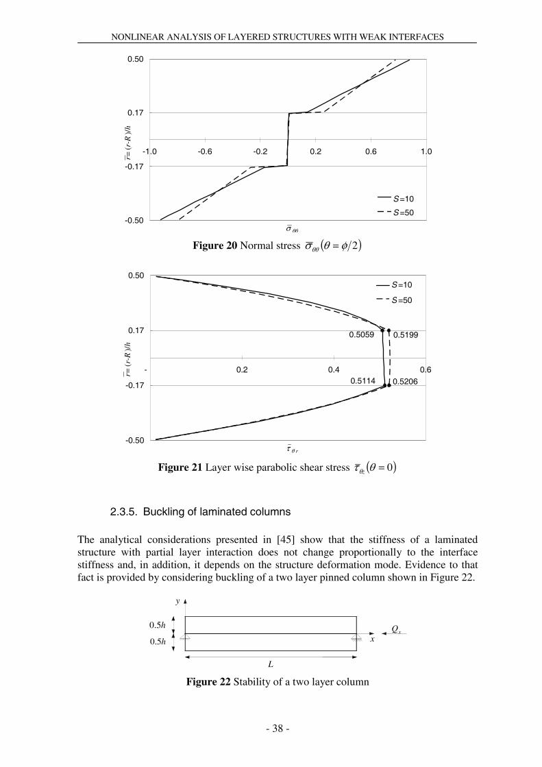
NONLINEAR ANALYSIS OF LAYERED STRUCTURES WITH WEAK INTERFACES
- 38 -
-0.50
-0.17
0.17
0.50
-1.0 -0.6 -0.2 0.2 0.6 1.0
σ θθ
r=(r
-R)/
h
s=10
s=50
S =10
S =50
Figure 20 Normal stress ( )2φθσθθ =
0.5059
0.5114
0.5199
0.5206
-0.50
-0.17
0.17
0.50
- 0.2 0.4 0.6
τ θ r
r=(r
-R)/
h
S=10
S=50
S =10
S =50
Figure 21 Layer wise parabolic shear stress ( )0=θτθz
2.3.5. Buckling of laminated columns The analytical considerations presented in [45] show that the stiffness of a laminated structure with partial layer interaction does not change proportionally to the interface stiffness and, in addition, it depends on the structure deformation mode. Evidence to that fact is provided by considering buckling of a two layer pinned column shown in Figure 22.
L
y
xQx
h5.0
h5.0
Figure 22 Stability of a two layer column

NONLINEAR ANALYSIS OF LAYERED STRUCTURES WITH WEAK INTERFACES
- 39 -
Under the assumption of Bernoulli kinematics at the layer level, [45] gives the consecutive buckling loads of the laminated column in the form:
)98( ),(][][ knPP nnk η∞=
where n is identification number of the consecutive buckling load (n = 1 corresponds to the Euler load), k is uniform interface stiffness, ][nP∞ are the buckling loads for the case of complete layer interaction and ),( knη describes buckling load evolution in terms of interface stiffness and deformation mode:
)99( 2
22
2
22][
1
),(
⎟⎠⎞
⎜⎝⎛+
⎟⎠⎞
⎜⎝⎛+
==∞
πϖπ
ϖβηπ
n
L
n
L
knL
EInP n
where 123bhI = is moment of beam cross section inertia for the case of complete layer
interaction and Ehk42 =ϖ . ∑=layer
layer II2β is a geometric parameter, which for the
chosen layer setup is 25.02 =β . Hence, the buckling loads of the considered beam setup are contained between two limits. When the interface rigidity assures complete layer interaction 1),(lim =∞→knη , and when the layers work independently
25.0)0,(lim =→knη . Assuming arbitrary values of geometric and material properties 100=L [mm], 1== bh [mm] and 410=E [MPa], Table V gives a comparison of the reference and present FE solution obtained with a uniform mesh of 30 elements. In order to enforce the Bernoulli's type of kinematics at the layer level, large layer shear stiffness 1010=G [MPa] is used in the FE model. It can be observed that the two solutions are in excellent agreement.
Table V Buckling loads of laminated beam-column with partial layer interaction
]1[][k
nk PP 1=n 2=n 3=n 4=n
reference ( )∞→k 1.00 4.00 9.00 16.00
FE ( )∞→k 1.00 4.00 9.00 16.01
reference ⎟⎟⎠
⎞⎜⎜⎝
⎛= 2
2
4L
Ehk
π 1.00 2.56 4.68 7.52
FE ⎟⎟⎠
⎞⎜⎜⎝
⎛= 2
2
4L
Ehk
π 1.00 2.56 4.68 7.53
The nonlinear dependence of laminated column stability on the interface stiffness and the deformation mode is further illustrated in Figure 23, where function ),( knη is plotted for four consecutive buckling modes.

NONLINEAR ANALYSIS OF LAYERED STRUCTURES WITH WEAK INTERFACES
- 40 -
0.250
0.375
0.500
0.625
0.750
0.875
1.000
0.000 0.002 0.004 0.006 0.008 0.010kb /E
η(k
,n)
n=1
n=2
n=3
n=4
n =1
n =2
n =3n =4
Figure 23 Laminated column stability in function of interface stiffness and deformation mode
Above considerations explicitly reveal the complexity of weak interface influence on laminated structure behaviour. Using a simple, linear interface constitutive model it is shown that the laminate rigidity is a nonlinear function of the interface stiffness, as well as the structure deformation character.
2.3.6. Beam-column with partial interaction Influence of shear deformability on the response of a simply supported beam-column considered in [20] and [19] is here investigated. Figure 24 shows the structure configuration and boundary conditions. The normal, compressive load Qx = 50 [kN] is distributed between the two layers accordingly to their axial stiffness (so that it does not induce any bending of straight column). A constant, transverse load q0= –1 [kN/m] is applied at the top of the second layer. The material properties correspond to wood and concrete in the bottom and the top layer respectively. As the referenced works did not address shear deformations, only Young’s modulus was specified for each layer: E(1) = 8 [GPa], E(2) = 12 [GPa]. In present work, two cases are considered. First, large shear stiffness at both layers is assumed. Hence, Bernoulli's type of layer kinematics is enforced and the reference solutions are reproduced. Next, influence of layer shear deformations is considered. For wood (the bottom layer), a representative ratio 20)1()1( =GE is assumed.
For concrete (the top layer), Poisson ratio is assumed to be ν(2) = 0.2. Hence, G(2) = 5 [GPa]. Partial interaction between the two layers is provided by shear connectors. In the referenced works, behaviour of these connectors is characterized using interface stiffness K = 50 [MPa]. Employing relation (39) the interface stiffness is here k(2) = 1 [GPa/m]. A uniform mesh of twenty elements is used.

NONLINEAR ANALYSIS OF LAYERED STRUCTURES WITH WEAK INTERFACES
- 41 -
x
b(2) = 0.30 [m]
b(1) = 0.05 [m]
h(1) = 0.15 [m]
h(2) = 0.05 [m]
q0 = -1 [kN/m]
L=4 [m]
[ ]kN5.12)1( =xQ
[ ]kN5.37)2( =xQ
)1(xQ
)2(xQ
concrete
wood
Figure 24 Beam-column with partial interaction
The linear results are compared in Table VI, where MAXv is maximum deflection, )(
MAXlayM ,
)(MAX
layN , )(MAX
layV are maximum layer stress resultants, and MAXF is maximum shearing force at the interface (F = Kg(2) = b(1)k(2)g(2)). Suppressing layer shear deformations, fine agreement with both reference solutions is obtained. Including shear deformations, deflection of the beam-column increases by 5%, but the interface slip/shear remains unchanged. As the rigidity of the bottom layer is significantly reduced (small shear stiffness) this layer is partially unloaded and the stresses in the top layer increase. Noteworthy, in geometric linear solution, there is no re-arrangement of layer normal force due to change of layer shear stiffness.
Table VI Geometric linear results
analytical,
[20] FE, [19]
FE, present, shear
deformations suppressed
FE, present, shear
deformations allowed
change due to shear deformations
[%]
MAXv [mm] –7.560 –7.559 –7.560 –7.935 5.0 )1(
MAXM [kNm] 0.4977 0.4978 0.4984 0.4915 –1.4 )2(
MAXM [kNm] 0.1659 0.1659 0.1661 0.1731 4.2 )1(
MAXN [kN] 0.863 0.862 0.884 0.884 0.0 )2(
MAXN [kN] –50.863 –50.862 –50.884 –50.884 0.0
MAXF [kN/m] 11.444 11.442 11.444 11.444 0.0
If Bernoulli kinematics at the layer level is enforced, the buckling load provided by present finite element formulation ]kN[0.271FEM
Bcr =Q corresponds closely to the value obtained
analytically in [20] ]kN[0.271refcr =Q . Allowing for layer shear deformation, the buckling
load decreases by 4.8% ( )]kN[9.257FEMTcr =Q .
Geometric nonlinear results are summarized in Table VII. As the relative displacements and rotations remain small, the linearized second-order analysis performed in [20] provides sufficiently accurate estimation of the geometric nonlinear effects. Noteworthy, stress re-

NONLINEAR ANALYSIS OF LAYERED STRUCTURES WITH WEAK INTERFACES
- 42 -
distribution taking shear deformations into account is more pronounced in geometric nonlinear analysis and affects layer normal forces and the interface shearing force.
Table VII Geometric nonlinear results
analytical,
[20] FE, [19]
FE, present, shear
deformations suppressed
FE, present, shear
deformations allowed
change due to shear deformations
[%]
MAXv [mm] –9.276 –9.274 –9.276 –9.851 6.2 )1(
MAXM [kNm] 0.6126 0.6157 0.6168 0.6151 –0.3 )2(
MAXM [kNm] 0.2054 0.2052 0.2056 0.2169 5.5 )1(
MAXN [kN] 3.897 3.918 3.954 4.145 4.8 )2(
MAXN [kN] –53.897 –53.933 –53.954 –54.145 0.4
MAXF [kN/m] 13.878 13.881 13.865 14.022 1.1
2.3.7. Uniform bending of cantilever This classical benchmark problem is adopted here in the form allowing for geometric nonlinear validation of laminated beam models with inter-layer slip. Figure 25 shows two adjacent cantilevers of equal length L. Bending moment applied to the tip of the first (bottom) beam is chosen to deform it into a quarter of a circle:
)100( ( )
)1(
3)1()1()1()1(
12R
hbEM =
where πLR 2)1( = is radius of the bottom beam midline, )1(E is the beam Young’s
modulus, and )1(b , )1(h are its width and thickness. Requiring the second beam to bend into a concentric arc defines the moment applied at the upper beam tip:
)101( ( )
)2(
3)2()2()2()2(
12R
hbEM =
where ( ))2()1(
21)1()2( hhRR +−= is the radius of the second beam midline, )2(E is the
second beam Young’s modulus, and )2(b , )2(h are its width and thickness. Provided that the two beams can slip freely, they should deform so that neither transverse separation nor transverse reactions develop. Slip at their interface is:
)102( ( ) xRR
RRhRxg
)2()1(
)2()1()1(
21)1()(
−−=
Using the proposed model, the beam assembly is represented as a two layer laminate with zero interface stiffness. Laminate reference line is chosen to be the bottom beam midline. Geometric and material properties are: L = 100 [mm], h(1) = 3h(2) = 3 [mm], b(1) = b(2) = 1 [mm], and 2E(1) = E(2) = 24.0 [GPa], 2G(1) = G(2) = 9.6 [GPa].

NONLINEAR ANALYSIS OF LAYERED STRUCTURES WITH WEAK INTERFACES
- 43 -
Table VIII gives the summary of numerical results obtained with a uniform mesh of ten elements. This, relatively coarse, mesh is sufficient to obtain fine agreement with the proposed benchmark. It can be observed, that the layer bending moments returned by present model do not correspond exactly to the applied load. Instead, they are redistributed proportionally to the layer bending stiffness:
)103( ( ) ( )( ) ( ))2()1()2()1(
)2()2()1()1(
)2()2()2(
)2()1()2()1(
)2()2()1()1(
)1()1()1(
29
2
29
27
MMMMIEIE
IEM
MMMMIEIE
IEM
+=++
=
+=++
=
This should be attributed to the use of linearized kinematic relations (unique transverse displacement throughout beam thickness) in the co-rotated element frame
R(2)
R(1)
L
90.00
92.90
x
y
)2(M
)1(M
Figure 25 Two cantilevers bent into concentric arcs (figure to scale)
Table VIII Uniform bending of the two layer assembly
Analytical FE (10 elements) error v(x=L) [mm] R(1)= 63.662 63.743 0.1 % u(x=L) [mm] R(1)–L= –36.338 –36.481 0.4 % g(x=L) [mm] 3.167 3.149 0.6 % M(x=0.5L)
[Nmm] M(1) = 424.115 M(2) = 32.435
M(1) = 425.064 M(2) = 31.486
0.2 % 2.9 %
max |V(x)| [N] V(1)= V(2)= 0.000 0.460 - max |N(x)| [N] N(1)= N(2)= 0.000 0.249 10–6 -
A minor perturbation of the FE results can be observed near the laminated beam tip, where the layer bending moments are driven to match the applied load system. As a result, a small transverse reaction is developed between the layers. This is manifested by appearance of opposing transverse layer forces (total transverse force remains zero). As this perturbation is due to the use of linearized kinematic relations, it remains small if small strain, moderate slip postulates are satisfied. For example, in the considered case, the ratio

NONLINEAR ANALYSIS OF LAYERED STRUCTURES WITH WEAK INTERFACES
- 44 -
of the maximum normal stress to the maximum shear stress ( )yLxlayxx ,max )( =σ /
( )yLxlayxy ,max )( =τ remains above 100 in both layer cross-sections.
2.3.8. Nonlinear buckling of sheathed walls A discussion on nonlinear buckling of a sheathed wood wall presented in [48] is here referenced. The wall setup consists of a simply supported stud with sheathing applied to one of its sides. The geometric parameters of the model are shown in Figure 26. Young’s modulus of the stud and the sheathing is E(1)= 7.84 [GPa] and E(2)= 4.90 [GPa], respectively. Wood shear deformations are not considered. Partial interaction of the two layers is obtained through nail connection characterized by a linear spring model (K = 49 [MPa]), which for present formulation is k = K/b(1) = 1.28947 [MPa/mm]. Employing uniform mesh of thirty elements and suppressing layer shear deformations by large (penalty) shear stiffness, the linear buckling load of FEM
crQ = 58.04 [kN] is obtained.
This corresponds closely to the reference analytical solution refcrQ = 58.19 [kN].
A notion of wall centre of compression introduced in [48] corresponds to the location in the wall thickness where the applied boundary condition system (the normal, compressive force Qx, and the supports) results in minimal deflection. Measured from the stud midline, the centre of compression for the considered wall is e ≈ 13.25 [mm] (it is worth noting that the location of the wall centre of compression depends on the interface stiffness).
e x
y
h (2)= 9 [mm]
h(1)= 88 [mm]
b(1)= 38 [mm]
b(2)= 341 [mm]
L= 2400 [mm]
xQ
Figure 26 Sheathed wall setup
Figure 27 shows dramatic change of the wall behaviour when boundary conditions are applied at three nearby locations: e = 15.00 [mm], e = 13.25 [mm] and e = 11.50 [mm]. Additionally, pronounced changes in deformation patterns for various load levels indicate considerable geometric nonlinear behaviour before buckling load is reached. Evidence to this is also provided in Table IX, where geometric linear and nonlinear deflections are compared.

NONLINEAR ANALYSIS OF LAYERED STRUCTURES WITH WEAK INTERFACES
- 45 -
-6.0
-5.0
-4.0
-3.0
-2.0
-1.0
0.00 240 480 720 960 1200 1440 1680 1920 2160 2400
x [mm]
v(x
) [m
m]
10 [kN]
20 [kN]
40 [kN]
Q x =10 [kN]
Q x =40 [kN]e =15.00 [mm]
Q x =20 [kN]
-0.8
-0.6
-0.4
-0.2
0
0.2
0.4
0.6
v(x
) [m
m]
10 [kN]
20 [kN]
40 [kN]Q x =40 [kN]
Q x =10 [kN]e =13.25 [mm]Q x =20 [kN]
0.0
1.0
2.0
3.0
4.0
5.0
6.0
v(x
) [m
m]
10 [kN]
20 [kN]
40 [kN]
Q x =10 [kN]
Q x =20 [kN]
Q x =40 [kN]
e =11.50 [mm]
Figure 27 Transverse deflection patterns for various boundary conditions
Table IX Deflections at wall centre, Qx = 40 [kN]
e = 15.00
[mm] e = 13.25
[mm] e = 11.50
[mm] present, linear, FE – 1.1355 0.3308 1.7972
present, nonlinear, FE – 4.4738 0.3823 5.2387 second order, analytical
[48] – 4.4805 0.3823 5.2451
An interesting effect of slip reversal near the buckling load for the case of e = 11.50 [mm] is shown in Figure 28.

NONLINEAR ANALYSIS OF LAYERED STRUCTURES WITH WEAK INTERFACES
- 46 -
0
10
20
30
40
50
60
-2 -1 0 1 2 3 4 5g (x=L ,e ,Q x ) [mm]
Qx [
kN]
e = 15 [mm]
e = 11.5 [mm]
e = 13.25 [mm]
e
e
e
Figure 28 Evolution of the interface slip at the wall tip, FE results
2.3.9. Nonlinear response of hyperstatic laminated beam Laminated structures with large degree of transverse anisotropy can exhibit substantial geometric nonlinear behaviour at small loads and deflections. This effect is here presented on the example of a two-layer, asymmetrically laminated plate strip considered in [49] and [17]. As shown in Figure 29, the laminate is pinned at two opposite ends and loaded with uniform transverse load q .
q
x
L
y
toth
Figure 29 Pinned-pinned, asymmetrically laminated plate
The geometric parameters are: width b=1.5 [in], thickness htot = 0.04 [in], length L = 9 [in]. The material properties are: E1 = 20 [msi], E2 = 1.4 [msi], ν = 0.3, G12 = G13 = G23 = 0.7 [msi], where direction 1 is parallel to the fibres, while 2 and 3 are perpendicular. Lamination scheme is (90/0). In present beam formulation, the plate effects are accounted for by specifying material properties of the layers as: ( )12212
)1( 1 νν−= EE , 23)1( GG = ,
( )21121)2( 1 νν−= EE , 12
)2( GG = . The interface slips are suppressed by large interface
stiffness 7)2( 10=k [msi/in]. A uniform mesh of 20 elements is used. For the supports located at the laminate midline, Figure 30 shows maximum plate deflection in function of the load amplitude. The geometric nonlinear effects appear instantly and are significant within small displacement range. Noteworthy, strong dependence on the load direction can be observed.

NONLINEAR ANALYSIS OF LAYERED STRUCTURES WITH WEAK INTERFACES
- 47 -
-1.2
-0.8
-0.4
0
0.4
0.8
-0.05 -0.04 -0.03 -0.02 -0.01 0 0.01 0.02 0.03 0.04 0.05q [psi]
v(L
/2)/
h tot
[49]
present linear
present nonlinear
Figure 30 Geometric nonlinear response of laminated plate, supports at plate midline
Figure 31 shows response of the laminate when the supports are displaced to the bottom of the first layer. The dependence on loading direction is more pronounced here and the snap-through type of behaviour is observed.
-2.4
-1.8
-1.2
-0.6
0
0.6
1.2
-0.05 -0.04 -0.03 -0.02 -0.01 0 0.01 0.02 0.03 0.04 0.05q [psi]
v(L
/2)/
h tot
[17]
present linear
present nonlinear
Figure 31 Geometric nonlinear response of laminated plate, supports at plate bottom
2.3.10. Steel-concrete bridge deck Addressed here is nonlinear behaviour of continuous steel-concrete bridge deck experimentally investigated by Teraszkiewicz [50] and further discussed in [29]. The bridge consists of steel I beam and an overlying concrete slab. Partial interaction between the two sub-components is enforced through uniformly spaced shear studs. Details of the configuration are shown in Figure 32.

NONLINEAR ANALYSIS OF LAYERED STRUCTURES WITH WEAK INTERFACES
- 48 -
yxQ
]mm[8.3352=L
L5.0
]mm[4.152
]mm[6.9]mm[1.6
]mm[2.76
x
]mm[6.609
]mm[3.60
Figure 32 Continuous steel-concrete bridge deck
Elasto-plastic behaviour of the steel I beam is governed by a bi-linear hardening law with Young’s modulus 5
st 1007.2=E [MPa], yield stress 08.307sty =σ [MPa] and hardening
ratio 005.0st =α . Additionally, a representative value of Poisson constant 3.0st =ν is
assumed in elastic domain. The I beam is subdivided into three layers corresponding to its flanges and the web. Interface slips between these layers are suppressed by large interface stiffness. The concrete slab is also subdivided into three layers, with the second layer corresponding to steel reinforcement of the slab. This layer is located at 80% of the total slab thickness and its thickness is chosen to obtain the area of reinforcement 16.445r =A [mm2]. Elasto-plastic behaviour of the reinforcement is governed by a bi-linear hardening law with Young’s modulus 5
r 1007.2=E [MPa], yield stress 321ry =σ [MPa] and hardening ratio
005.0r =α . Poisson constant 3.0r =ν is assumed in elastic domain of the reinforcement. Modelling inelastic behaviour of the concrete layers requires special attention. Following [29], the concrete is assumed not to possess any tensile strength and its behaviour in compression is characterised by an initial modulus 8.16270c =−E [MPa], maximum
compressive stress 677.40cu −=−σ [MPa] and compressive crushing strain 006.0ccr −=−ε
where the stress level instantly drops to zero. The above characteristic is used here only for the normal stress-strain relationship, whereas the shear stress-strain relation is assumed linear, symmetric (with shear modulus )1(2 ccc ν+= −EG and 25.0c =ν arbitrarily
assumed). This grossly simplified approach seems, nevertheless, sufficient in this particular problem where shear deformations of the concrete slab are negligible. A more rigorous approach would necessitate change of yield criterion in the radial return development of paragraph 2.1.3. However, it can be observed that assuming lack of tensile concrete strength leads to instant failure of the top layer at the mid support of the deck ( )Lx = . This would result in null tangent constitutive matrix for this layer and, in consequence, singular stiffness matrix would be obtained. Thus, in order to stabilize numerical solution, some small shear stiffness would have to be defined for the failed top layer of concrete. Nonlinear behaviour of shear studs, providing interaction between the steel beam and the concrete slab, is idealized using a power law in the form:
)104( ( )intuint1intufgk
eff−−=
where g [mm] is the interface slip, 82.5int =uf [MPa] is the ultimate load carrying
capacity of the interface and 54.27int =k [MPa/mm] is the initial tangent modulus. [29]
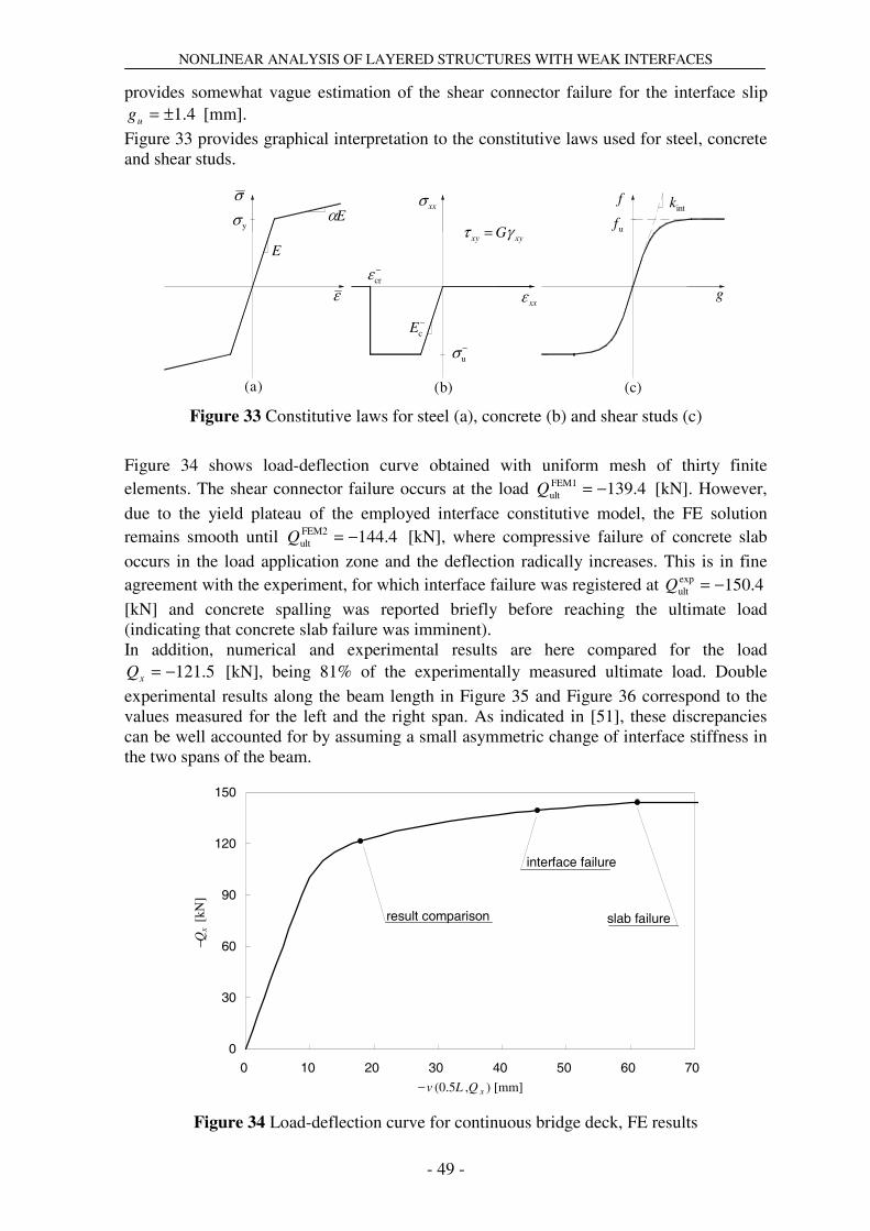
NONLINEAR ANALYSIS OF LAYERED STRUCTURES WITH WEAK INTERFACES
- 49 -
provides somewhat vague estimation of the shear connector failure for the interface slip 4.1±=ug [mm].
Figure 33 provides graphical interpretation to the constitutive laws used for steel, concrete and shear studs.
ε
E
σ
)a(
−crε
Eαyσ
)b( )c(
−cE
xxσ
xxε
−uσ
g
fintk
ufxyxy Gγτ =
Figure 33 Constitutive laws for steel (a), concrete (b) and shear studs (c)
Figure 34 shows load-deflection curve obtained with uniform mesh of thirty finite elements. The shear connector failure occurs at the load 4.139FEM1
ult −=Q [kN]. However,
due to the yield plateau of the employed interface constitutive model, the FE solution remains smooth until 4.144FEM2
ult −=Q [kN], where compressive failure of concrete slab
occurs in the load application zone and the deflection radically increases. This is in fine agreement with the experiment, for which interface failure was registered at 4.150exp
ult −=Q
[kN] and concrete spalling was reported briefly before reaching the ultimate load (indicating that concrete slab failure was imminent). In addition, numerical and experimental results are here compared for the load
5.121−=xQ [kN], being 81% of the experimentally measured ultimate load. Double
experimental results along the beam length in Figure 35 and Figure 36 correspond to the values measured for the left and the right span. As indicated in [51], these discrepancies can be well accounted for by assuming a small asymmetric change of interface stiffness in the two spans of the beam.
0
30
60
90
120
150
0 10 20 30 40 50 60 70
− v (0.5L ,Q x ) [mm]
−Qx [
kN]
interface failure
result comparison slab failure
Figure 34 Load-deflection curve for continuous bridge deck, FE results

NONLINEAR ANALYSIS OF LAYERED STRUCTURES WITH WEAK INTERFACES
- 50 -
-25
-20
-15
-10
-5
0
0.0 558.8 1117.6 1676.4 2235.2 2794.0 3352.8
x [mm]
v(x
) [m
m]
FE
EXPERIMENT
Figure 35 Transverse deflection at 5.121−=xQ [kN]
-0.6
-0.3
0
0.3
0.6
0.0 558.8 1117.6 1676.4 2235.2 2794.0 3352.8
x [mm]
g(x
) [m
m]
FE
EXPERIMENT
Figure 36 Interface slip at 5.121−=xQ [kN]
It can be added that the geometric nonlinear effects in present analysis are negligible. This can be deduced from Figure 34, showing that the transverse deflections remain small until ultimate state is reached.

NONLINEAR ANALYSIS OF LAYERED STRUCTURES WITH WEAK INTERFACES
- 51 -
2.4. Summary for beam formulation The above development provides a model suitable for geometric and material nonlinear analysis of laminated beams with inter-layer slips. Remarkable property of the proposed formulation is the balance between simplicity (computational efficiency) and quality of the results. Two properties deserve particular attention. First, evidence is provided to the robustness of the co-rotational formulation in dealing with large displacements of laminated beams. Second, a relatively simple model based on FSDT is shown to provide reliable transverse shear stress distributions. It should also be underlined that the development is made for an arbitrary number of layers. Hence, remarkable flexibility is provided for modelling complex engineering problems. Performance of the proposed model is tested in a series of demanding numerical tests and the FE results are found to be in satisfactory agreement with all benchmarks. When compared to classical beam formulations, the proposed laminated beam model offers significant improvement in modelling capabilities. As usually in such cases, this is obtained at the expense of greater susceptibility to numerical problems. An overview of these problems is provided here. The discussion is sub-divided into three main categories: reliability of layer stress/strain fields, layer interface problems and singularity of numerical solution. As in 2D elasticity, present model may return singular stress distributions. This can occur in presence of point-wise bending moment, point-wise normal force, or equivalently for normal reaction developed at a pin support. In such case, performing transverse refinement, singular stress concentration is revealed. If this refinement is excessive, numerical solution using higher order elements may become ill conditioned. It is manifested by perturbation of the bending moment distribution at the layer where the point load (or support) is applied. This is due to the fact that the layer bending stiffness diminishes with cube of the layer thickness, while normal and shear stiffness are linear functions of the thickness. Noteworthy, this perturbation spreads through the entire layer (beam) length. On the other hand, the layer-wise shear stress field is not prone to singular concentrations. This is due to uniqueness of transverse displacement in laminated beam thickness. However, this property leads to poor quality of shear stress estimation at built-in supports. Suppressing transverse displacements and layer rotations at the same time is observed to drive layer shear stress re-distribution proportional to layer shear rigidity. Hence, in vicinity of this type of boundary condition, transverse shear stress distribution provided by present formulation is not reliable. Notably, this rearrangement has no effect on estimation of the global transverse force. Using linearized kinematic relations, the interface slip variable is effectively the axial component of the real slip. Hence, if the reference configuration is curved, its approximation by assembly of straight elements leads to inconsistency of interface slip interpretation at element junctions. As a result, a small perturbation of interface slip distribution can be observed for higher order elements (with at least quadratic variation of interface slip within element). It should be noted that, if the small-strain / shallow-curvature assumptions are satisfied, the terms simplified in the linearization of kinematic relations are negligible, and hence, solution perturbation remains small. Another problem associated with interface is the possibility of numerical solution ill conditioning due to applying excessive interface stiffness with respect to layer shear stiffness. This might take place if large interface stiffness is employed to simulate complete layer interaction. However, performed numerical experiments show that the developed elements support well order of interface stiffness three to four times larger than the order of layer shear stiffness. This is usually sufficient to suppress the slippage effects to negligible level.

NONLINEAR ANALYSIS OF LAYERED STRUCTURES WITH WEAK INTERFACES
- 52 -
Using the proposed formulation special attention need to be paid to avoiding singularity of the FE solution. Two major cases can be distinguished here. If element reference layer or one of external layers has zero stiffness, the element stiffness matrix has zero diagonal terms. This property is of particular importance in material nonlinear analysis where such condition may occur due to layer yielding. Interestingly, in all other cases (zero stiffness of non reference, internal layers and zero interface stiffness), the element stiffness matrix does not have zero diagonal terms. This is due to the additive character of the kinematic relations. Another important aspect is preventing rigid-body-motion within laminate. Though this problem can be easily eradicated, its presence is not always evident. For example, note that having zero interface stiffness or zero layer stiffness can be admissible in a cantilever but will lead to singular stiffness matrix for a simply supported configuration.

NONLINEAR ANALYSIS OF LAYERED STRUCTURES WITH WEAK INTERFACES
- 53 -
3. Plates Proposed here is a model of laminated plate with weak layer interfaces. The development is largely similar to the laminated beam formulation obtained in previous paragraphs. Hence, presented are only its key components and the main accent is put on novel aspects. In sharp contrast to the beam model, present development is restricted to moderate displacements and the Total Lagrangian FE formulation. This is due to the fact that the use of the co-rotational FE formulation, to account for large rigid-body-motion of a 2D element, would require the shallow shell approach rather than the plate one. The material nonlinear effects are also not considered. This however can be straightforwardly included noting the well-known Reissner-Mindlin plate formulation at the layer level.
3.1. Theoretical development Laminated plate is here assumed to lie in x-y plane and layer stacking sequence follows the z ordinate direction. Layers are of uniform thickness )(layh . Independent variable set consists now of 14 +Nlay components. These are, three reference plane displacements
( ( )yxu , , ( )yxv , , ( )yxw , ), Nlay2 layer cross-section rotations ( ( )yxlayx ,)(θ , ( )yxlay
y ,)(θ )
and ( )12 −Nlay interface slips ( ( )yxg intx ,)( , ( )yxg int
y ,)( ). Right-Hand-Rule (R-H-R) is used
for sign convention of layer cross-section rotations.
3.1.1. Kinematic relations In 2D problems the FSDT is known as the Reissner-Mindlin plate theory. Applying it at the layer level, the following linearized kinematic relations can be written:
)105(
( ) ( ) ( )( ) ( ) ( )( ) ( )yxwzyxw
yxzyxvzyxv
yxzyxuzyxu
laylay
layx
laylaylaylay
layy
laylaylaylay
,,,
,,,,
,,,,
)()(
)()()()()(
)()()()()(
≈
−≈
+≈
θ
θ
where for the reference layer (lay = ref):
)106( ( ) ( ) ( )( ) ( ) ( )yxzyxvyxv
yxzyxuyxuref
xrefref
refy
refref
,,,
,,,)()(
ecc)(
)()(ecc
)(
θ
θ
+≈
−≈
for the layers above the reference layer (lay > ref):

NONLINEAR ANALYSIS OF LAYERED STRUCTURES WITH WEAK INTERFACES
- 54 -
)107(
( ) ( ) ( ) ( )
( ) ( )
( ) ( ) ( ) ( )
( ) ( )yxgyxh
yxhyxhyxvyxv
yxgyxh
yxhyxhyxuyxu
lay
refi
iy
lay
refl
lx
l
layx
layrefx
refreflay
lay
refi
ix
lay
refl
ly
l
layy
layrefy
refreflay
,,
,,,,
,,
,,,,
1
)(
1
)()(
)()(21)()(
21)()(
1
)(
1
)()(
)()(21)()(
21)()(
∑∑
∑∑
+=+=
+=+=
++
+−+≈
+−
++−≈
θ
θθ
θ
θθ
and finally, for the layers below the reference layer (lay < ref):
)108(
( ) ( ) ( ) ( )
( ) ( )
( ) ( ) ( ) ( )
( ) ( )yxgyxh
yxhyxhyxvyxv
yxgyxh
yxhyxhyxuyxu
lay
refi
iy
lay
refl
lx
l
layx
layrefx
refreflay
lay
refi
ix
lay
refl
ly
l
layy
layrefy
refreflay
,,
,,,,
,,
,,,,
1
)1(
1
)()(
)()(21)()(
21)()(
1
)1(
1
)()(
)()(21)()(
21)()(
∑∑
∑∑
−=
+
−=
−=
+
−=
−−
++−≈
−+
+−+≈
θ
θθ
θ
θθ
In the above, layer index ref and local ordinate )(
eccrefz are used to define location of the
reference plane in laminate thickness. Interface slips are again taken as measures in deformed configuration. Using the small-strain and the moderate-slip assumptions )(int
jg
( )Nlayintyxj ,...,3,2;, == is here defined as a line measure of interface slip in direction j . Thus, the norm of the total interface slip can be written as:
)109( ( ) ( )[ ] ( )[ ]2)(2)()( ,,, yxgyxgyxg iy
ix
i +=
It should be noted that )(i
xg and )(iyg constitute a 2D vector field dependent on the choice
of the reference frame. In here developed plate formulation the reference frame may at most be subject to 1D rotation (about the z axis). Thus, transformation of so defined interface displacement field does not pose a particular problem. On the other hand, it can be deduced that constructing consistent transformation of this field can be rather cumbersome when the reference frame is subject to arbitrary 3D rotations (as it is the case in the co-rotational shallow shell formulation).

NONLINEAR ANALYSIS OF LAYERED STRUCTURES WITH WEAK INTERFACES
- 55 -
3.1.2. Geometric relations The layer-wise strain field of the von Kármán type can now be written as:
)110(
⎪⎪⎪⎪⎪⎪⎪
⎩
⎪⎪⎪⎪⎪⎪⎪
⎨
⎧
∂∂+
∂∂=
∂∂+
∂∂=
⎟⎟⎠
⎞⎜⎜⎝
⎛∂
∂∂
∂+∂
∂+∂
∂=
⎟⎟⎠
⎞⎜⎜⎝
⎛∂
∂+∂
∂=
⎟⎟⎠
⎞⎜⎜⎝
⎛∂
∂+∂
∂=
z
v
y
w
z
u
x
w
y
w
x
w
x
v
y
u
y
w
y
v
x
w
x
u
laylaylay
yz
laylaylay
xz
laylaylaylaylay
xy
laylaylay
yy
laylaylay
xx
)()()(
)()()(
)()()()()(
2)()()(
2)()()(
2
1
2
1
γ
γ
γ
ε
ε
It should be noted here that in the Total-Lagrangian formulation, derivatives are performed with respect to the initial reference frame and total displacements are used. To simplify further developments, relation (110) is re-cast here in the matrix notation:
)111( vK)(
0)( εεε += laylay
where:
)112( [ ])()()()()(T)( layyz
layxz
layxy
layyy
layxx
lay γγγεε=ε
)113(
⎥⎥⎥⎥⎥⎥⎥⎥⎥⎥⎥⎥
⎦
⎤
⎢⎢⎢⎢⎢⎢⎢⎢⎢⎢⎢⎢
⎣
⎡
−∂∂
+∂∂
⎟⎟⎠
⎞⎜⎜⎝
⎛
∂∂−
∂∂
+∂
∂+∂
∂∂
∂−∂
∂∂
∂+
∂∂
=
)(
)(
)()()(
)()(
)()(
)(
)()(
)(
)(0
layx
layy
layx
layylay
laylay
layxlay
lay
layylay
lay
lay
y
wx
wxy
zx
v
y
u
yz
y
vx
zx
u
θ
θ
θθ
θ
θ
ε
and
)114( ⎥⎥⎦
⎤
⎢⎢⎣
⎡⎟⎟⎠
⎞⎜⎜⎝
⎛∂∂
∂∂
⎟⎟⎠
⎞⎜⎜⎝
⎛∂∂
⎟⎠⎞
⎜⎝⎛∂∂= 00
2
1
2
122
TvK y
w
x
w
y
w
x
wε

NONLINEAR ANALYSIS OF LAYERED STRUCTURES WITH WEAK INTERFACES
- 56 -
3.1.3. Constitutive relations In present development only linear constitutive relations are considered. At the layer level, these can be written in the following compact form:
)115( )()()( laylaylay εDσ =
where )(layσ and )(layε are vectors grouping layer stress and strain components and )(layD is
layer constitutive matrix. Assuming that layer material is linear, orthotropic and that its principal axes coincide with axes of the plate reference frame, the Hooke’s law for plane stress problems states:
)116(
⎥⎥⎥⎥⎥⎥
⎦
⎤
⎢⎢⎢⎢⎢⎢
⎣
⎡
⎥⎥⎥⎥⎥⎥⎥⎥⎥
⎦
⎤
⎢⎢⎢⎢⎢⎢⎢⎢⎢
⎣
⎡
−−
−−
=
⎥⎥⎥⎥⎥⎥
⎦
⎤
⎢⎢⎢⎢⎢⎢
⎣
⎡
)(
)(
)(
)(
)(
)(
)(
)(
)()(
)(
)()(
)()(
)()(
)()(
)()(
)(
)(
)(
)(
)(
)(
0000
0000
0000
00011
00011
layyz
layxz
layxy
layyy
layxx
layyz
layxz
layxy
layyx
layxy
layy
layyx
layxy
layy
layxy
layyx
layxy
layx
layyx
layyx
layxy
layx
layyz
layxz
layxy
layyy
layxx
G
G
G
EE
EE
γγγεε
ννννν
ννν
νν
τττσσ
where )()()()( lay
ylay
xylay
xlay
yx EE νν = in order to satisfy the requisite of the constitutive matrix
symmetry. If material principal axes do not coincide with the plate reference frame, the constitutive matrix needs to be rotated to this frame, see e.g. [1]. Interface constitutive relation is here expressed using analogous matrix notation:
)117( )()()( intintint gkf =
where
)118( ⎥⎦
⎤⎢⎣
⎡=⎥
⎦
⎤⎢⎣
⎡= )(
)()(
)(
)()( and int
y
intxint
inty
intxint
g
g
f
fgf
As in case of beams, reactions developed at an interface are interpreted here as the interface shear stresses )(intf ]m/N[ 2 . Assuming that interface is linear, orthotropic, with
two principal axes corresponding to the laminated plate reference frame axes, the constitutive matrix )(intk takes the following form:
)119( ⎥⎦
⎤⎢⎣
⎡= )(
)()(
0
0int
y
intxint
k
kk
As in the case of layer Hooke’s law, there is no coupling assumed between two interface shear components.
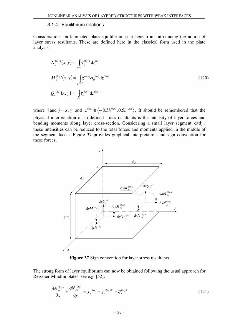
NONLINEAR ANALYSIS OF LAYERED STRUCTURES WITH WEAK INTERFACES
- 57 -
3.1.4. Equilibrium relations Considerations on laminated plate equilibrium start here from introducing the notion of layer stress resultants. These are defined here in the classical form used in the plate analysis:
)120(
( )
( )
( ) ∫
∫
∫
=
=
=
)(
)(
d,
d,
d,
)()(
)()()(
)()(
lay
lay
(lay)
z
(lay)layiz
layi
z
(lay)layij
laylayij
z
(lay)layij
layij
zyxQ
zzyxM
zyxN
τ
σ
σ
where yxji , and = and (lay)(lay)(lay) hhz 5.0,5.0−∈ . It should be remembered that the
physical interpretation of so defined stress resultants is the intensity of layer forces and bending moments along layer cross-section. Considering a small layer segment yxdd , these intensities can be reduced to the total forces and moments applied in the middle of the segment facets. Figure 37 provides graphical interpretation and sign convention for these forces.
x
y
yd
xd
z
)(d layxxyN
)(d layxyyN
)(d layxyyM)(d lay
xxyM
)(d layyyxN
)(d layyyxM
)(d layyxQ
)(d layxyQ
)(layh)(d lay
yxxN
)(d layyxxM
Figure 37 Sign convention for layer stress resultants
The strong form of layer equilibrium can now be obtained following the usual approach for Reissner-Mindlin plates, see e.g. [52]:
)121( )()1()()()(
layx
layx
layx
layxy
layxx qff
y
N
x
N −−=∂
∂+
∂∂ +

NONLINEAR ANALYSIS OF LAYERED STRUCTURES WITH WEAK INTERFACES
- 58 -
)122( )()1()()()(
layy
layy
layy
layyy
layxy qff
y
N
x
N−−=
∂∂
+∂
∂ +
)123( ( ))1()()(21)(
)()(++−=
∂∂
+∂
∂ layx
layx
laylayx
layxy
layxx ffhQ
y
M
x
M
)124( ( ))1()()(21)(
)()(++−=
∂∂
+∂
∂ layy
layy
laylayy
layyy
layxy ffhQ
y
M
x
M
)125( )()1()()()(
layz
layz
layz
layy
layx qpp
y
Q
x
Q −−=∂
∂+
∂∂ +
where )(lay
xq , )(layyq , )(lay
zq refer to components of distributed loading applied at the mid-
plane of a the layer segment yxdd . As usual in plate analysis, distributed bending moments
are not considered. )(lif and )(l
zp ( )1, += laylayl are interface shear and normal stresses at
layer top and bottom. Analogously to the preceding beam development, normal interface stresses can be eliminated from laminated plate equilibrium by summing up relations (125):
)126( zyx q
y
Q
x
Q −=∂∂
+∂∂
where
)127( ∑∑∑===
===Nlay
lay
layzz
Nlay
lay
layyy
Nlay
lay
layxx qqQQQQ
1
)(
1
)(
1
)( ;;
Hence, (121) to (124) and (126) constitute 14 +Nlay equilibrium relations necessary to resolve the proposed laminated plate model. Following the derivation scheme presented for laminated beams, the weak equilibrium of laminated plate can be provided in the classical form of the Principle of Virtual Work ( )0=+ extint WW δδ . In this case, the virtual work of internal forces takes the following
form:
)128( ( ) ∑∫∑ ∫==
+=Nlay
int A
intintNlay
lay Ω
laylaylay AΩWlay 2
)(T)(
1
)()(T)( dd)(
fgσε δδδ int
In the above relation all layers are assumed of identical shape. Thus, all interfaces have equal area A and layer volume is )()( laylay AhΩ = . The virtual work of external forces is:

NONLINEAR ANALYSIS OF LAYERED STRUCTURES WITH WEAK INTERFACES
- 59 -
)129(
( ) ( )∫ ∫
∑∫
∫
∑∫
∫
∫∑∫
−−
+
⎪⎪
⎭
⎪⎪
⎬
⎫
⎪⎪
⎩
⎪⎪
⎨
⎧
−
+−
−
+
⎪⎪
⎭
⎪⎪
⎬
⎫
⎪⎪
⎩
⎪⎪
⎨
⎧
+
++
−
+−+−=
=
=
=
σ σ
σ
σ
σ
σ
σσ
σ
σ
σ
σ
δδ
δθδθ
δθδθ
δδ
δδ
δδδδ
x y
y
x
y
x
Γ Γyyxx
Nlay
lay
Γy
layxy
layy
layyy
layx
Γx
layxx
layy
layxy
layx
Nlay
lay
Γy
layyy
laylayxy
lay
Γx
layxy
laylayxx
lay
A
z
Nlay
lay A
layy
laylayx
lay
ΓQwΓQw
ΓMM
ΓMM
ΓNvNu
ΓNvNu
AqwAqvquW
dd
d
d
d
d
dd
1 )()()()(
)()()()(
1 )()()()(
)()()()(
1
)()()()(ext
As the shape of all layers is identical, a simplified notation iΓ is used here to denote layer
mid-plane edge with normal direction i=x,y. Thus, yΓ x dd = and xΓ y dd = . Additional
index σ is used to underline the fact that considered are only edge portions with imposed natural boundary conditions. )(lay
ijN , )(layijM and iQ are the imposed force and bending
moment intensities on relevant edge segment σiΓ .

NONLINEAR ANALYSIS OF LAYERED STRUCTURES WITH WEAK INTERFACES
- 60 -
3.2. Finite element development Presented in this section is the development of laminated plate FE matrix formulation and its implementation in the form of four node quadrilateral element.
3.2.1. Total-Lagrangian finite element formulation It should be remembered that present development is made in view of geometric nonlinear Total-Lagrangian FE formulation. Hence, integration of element vectors and matrices is performed over the initial element configuration and total displacements are used at all times. Typical plate elements have either triangular or quadrilateral topology. In the simplest case, these are the three node triangle and the four node quadrilateral. Thus, the vector of plate element degrees of freedom d can be written as:
)130( [ ],...,, TC
TB
TA
T dddd =
where md (m = A,B,C,...) are vectors of nodal DOFs. In present development these can be
written in the following form:
)131( [ ])()()()()1()1(T ,,,,...,,,,, Nlaymy
Nlaymx
Nlaymy
Nlaymxmymxmmmm ggwvu θθθθ=d
Choosing element topology implies the interpolation scheme used to approximate the element kinematic field (105):
)132( ( ) ( )dNu yxyx ,, =
where [ ])()()()()1()1(T ,,,,...,,,,, Nlayy
Nlayx
Nlayy
Nlayxyx ggwvu θθθθ=u is the transpose of a 14 +Nlay
vector of independent kinematic variables. If Lib is used to denote the total number of element degrees of freedom (dimension of vector d ), the matrix of element shape functions ( )yx,N is ( ) LibNlay ×+14 . The element virtual displacement and virtual strain fields can be written in the form analogous to the beam formulation:
)133( ( ) dNddu
u δδδ yx,=∂∂=
)134( ( ) ddBdd
εε δδδ ,,, )()(
)()( laylay
laylay zyx=
∂∂
=
Following the strain decomposition given in (111) , the matrix )(layB can be decomposed
into linear and geometric nonlinear components:
)135( ( ) ( ) ( )dBBdB ,,,,,,, vK)()(
0)()( yxzyxzyx laylaylaylay +=

NONLINEAR ANALYSIS OF LAYERED STRUCTURES WITH WEAK INTERFACES
- 61 -
It should be remembered that in present plate formulation there are five strain components. Hence, dimension of all B matrices is Lib×5 . To simplify further development, yet one more matrix definition is here introduced:
)136( ( ) dNdd
gg δδδ yxint
g
intint ,)(
)()( =
∂∂=
where ( )yxint
g ,)(N , Nlayint ,...,2= are Lib×2 sub-matrices of ( )yx,N , containing only
interpolation functions used for given interface. Employing relations (133) to (136), the virtual work of element internal and external forces can now be expressed as:
)137( ( ) extextintint QddQd TT and δδδδ −== WW
where the vector of element internal forces is:
)138(
( ) ( ) ( ) ( ) ( )∑ ∫
∑ ∫
=
= Ω
+
+=
Nlay
int A
intintg
Nlay
lay
laylaylaylaylay
Ayxyx
Ωzyxzyxlay
2
)(T)(
1
)()()()(T)(
d,,,
d,,,,,,)(
dfN
dσdBdQint
As in the preceding beam formulation, the vector of element external forces extQ is to be
established with the aid of layer-wise kinematic relations. Despite its lengthiness, this operation does not bring in any novel aspects and hence it is not discussed. Passage from element to structure level and obtaining matrix formulation for the Newton-Raphson iterative solution algorithm adhere to the development presented for the laminated beam formulation. Hence, for the sake of completeness, only the final form of element tangent stiffness matrix is recalled here:
)139( ( ) ( ) ( )dKdKdK σ+=TAN
where matrix ( )dK is now defined as:
)140(
( ) ( ) ( ) ( ) ( )∑ ∫
∑ ∫
=
= Ω
+
=
Nlay
int A
intg
intintg
Nlay
lay
laylaylaylaylaylay
Ayxyx
Ωzyxzyxlay
2
)()(T)(
1
)()()()()(T)(
d,,
d,,,,,,)(
NkN
dBDdBdK
Analogously to the beam formulation, evaluation of the initial stress matrix ( )dKσ can be
considerably simplified:
)141(
( ) ( ) ( )
( )∫ ∑
∑ ∫
⎪⎭
⎪⎬⎫
⎪⎩
⎪⎨⎧
⎟⎟⎠
⎞⎜⎜⎝
⎛∂∂
=
=⎭⎬⎫
⎩⎨⎧
∂∂=
=
= Ω
A
Nlay
lay
layij
ij
Nlay
lay
laylaylay
AyxN
Ωzyxyx
lay
d,,
d,,,,,
1
)(2
2
1
)()()(TvK
)(
dd
ε
dσd
dBdKσ

NONLINEAR ANALYSIS OF LAYERED STRUCTURES WITH WEAK INTERFACES
- 62 -
where xyyyxxij ,,= . Hence, the initial stress matrix is obtained as a sum of three sparse
matrices 2
2
d
ε∂∂ ij multiplied by sums of relevant layer force intensities.
Analogously to the preceding beam formulation, it can be noted that present formulation can be down-graded to address geometric-linear problems, as well as, linearized buckling. Alternatively, using some well-known material non-linear approaches for Reissner-Mindlin plates, e.g. [33], the above matrix formulation can be trivially extended to include material non-linear effects at the layer level.
3.2.2. Element topology and mapping Element chosen for FE implementation of the developed plate formulation is the four node quadrilateral with bi-linear interpolation of all kinematic variables. Figure 38 shows an arbitrary element shape in global reference frame (X-Y-Z). The element is defined by four corner nodes 1, 2, 3, and 4. Auxiliary points A, B, C and D are established as the element edges mid-points. The x axis of the element local frame (x-y-z) is chosen along segment D-B, with origin at point O. The y axis is orthogonal to the x axis, and lies in plane defined by segments A-C and D-B. The z axis is then constructed as orthogonal to x and y axes. As indicated in [53], this choice of element local frame allows for an elegant treatment of warped element configuration. Hence, it is particularly suitable for future extension to the co-rotational laminated shell formulation.
2
Z
Y
X
x
y
η
ξ
4
C
3
D
1
A
B1 A 2
B
3C4
D
O
O
Figure 38 Quadrilateral plate element reference frame and mapping
Figure 38 shows also natural element configuration defined in non-dimensional (natural) reference frame (ξ-η-ζ). In this configuration the element shape functions are defined as:
)142( ( ) ( )( )nnnN ηηξξηξ ++= 114
1,

NONLINEAR ANALYSIS OF LAYERED STRUCTURES WITH WEAK INTERFACES
- 63 -
where 4,3,2,1=n refers to the element nodes and 1, ±=nn ηξ are non-dimensional co-
ordinates of these nodes. Element spatial co-ordinates can now be mapped using the element shape functions and nodal co-ordinates:
)143( ( ) ( )∑=
=4
1nnnN xx ξξ
where [ ]yx,T =x and [ ]ηξ ,T =ξ . Layer transverse ordinate can be trivially expressed as:
)144( ζ2
)()(
laylay h
z =
In order to complete the discussion on element mapping, spatial derivatives need to be expressed in the natural reference frame. This can be written in the following compact form:
)145( xx ∂∂
∂∂=
∂∂ ξ
ξ
where x∂∂ξ is defined in the usual manner (compare to e.g. [54]):
)146( ξηηξξξ
ηη yxyxJxy
xy
J,,,,and
,,
,,11
−=⎥⎦
⎤⎢⎣
⎡−
−=⎟
⎠
⎞⎜⎝
⎛∂∂=
∂∂
−
ξξξ
ξ xx
and (143) stipulates that:
)147( ⎥⎦
⎤⎢⎣
⎡=
∂∂
ηξ
ηξ
yy
xx
,,
,,
ξx
3.2.3. Rotation of element vectors and matrices As shown in Figure 38 base vectors of the global and element reference frames are not necessarily parallel. Hence, in order to perform element assembly (aggregation), element vectors and matrices need to be rotated to a common, e.g. global, frame. In present plate formulation this is 1D rotation about z||Z axis. Hence, constructing appropriate rotation matrix does not pose particular problem. However, it should be underlined here that this transformation now applies also to the interface slip field. For example, recall the form of element kinematic variable vector given in (132):
)148( [ ])()()()()1()1(T ,,,,...,,,,, Nlayy
Nlayx
Nlayy
Nlayxyx ggwvu θθθθ=xu
Rotation of this vector to the global co-ordinates can be expressed as:
)149( xX uRu T=
where R is the rotation matrix from the global frame to element frame. This matrix has the following form:

NONLINEAR ANALYSIS OF LAYERED STRUCTURES WITH WEAK INTERFACES
- 64 -
)150(
⎥⎥⎥⎥⎥⎥⎥⎥⎥⎥⎥⎥⎥⎥
⎦
⎤
⎢⎢⎢⎢⎢⎢⎢⎢⎢⎢⎢⎢⎢⎢
⎣
⎡
−
−
−
−
=
cs
sc
cs
sc
cs
sc
cs
sc
0000000
0000000
0000000
0000000
0000000
0000000
000000100
0000000
0000000
L
L
L
L
MMMMOMMMMM
L
L
L
L
L
R
where ( )zc αcos= , ( )zs αsin= and zα is the angle measured from the global X axis to the x axis of element frame.
3.2.4. Management of numerical locking Four node quadrilateral elements based on the Reissner-Mindlin formulation are subject to shear locking. As in beam formulation, this can be circumvented by reduced integration of transverse shear components. However, the rank deficiency of element stiffness matrix caused by this operation has severe impact on plate element behaviour, see e.g. [38]. Therefore, in present development, an assumed strain method is chosen to alleviate the shear locking. The adopted approach follows the one proposed by Bathe and Dvorkin in [55]. This prevents appearance of spurious zero-energy modes and improves results for non-rectangular element configurations. Moreover, the assumed shear strains are integrated using the same scheme as the normal strains, e.g. 2x2 Gaussian scheme. Hence the method is also suitable in material nonlinear analysis. The assumed shear strain field proposed by Bathe and Dvorkin is defined in natural co-ordinate system of the element. Each component of transverse shear strain is taken as constant in one direction and linear in the other one. They are required to comply with the shear stress field computed from the displacement field at selected points along the element edges and read:
)151( ⎪⎩
⎪⎨
⎧
−++=
−++=
DB
AC
2
1
2
12
1
2
1
ηζηζηζ
ξζξζξζ
γηγηγ
γηγηγ
where ηζξζ γγ , are the assumed transverse shear strains and m
ηζmξζ γγ , are the shear strains
evaluated from the kinematic field at points Dand C B,A,=m . As the presented development is to be applied at each layer of laminated plate, the layer index is here omitted to simplify the notation. Element deformation field in the element natural co-ordinate system is evaluated as the linear part of the Green-Lagrange strain measure:
)152( ( )lklkkl gggg 001121 −=ε

NONLINEAR ANALYSIS OF LAYERED STRUCTURES WITH WEAK INTERFACES
- 65 -
where ζηξ ,,, =lk and lk gg 00 , are co-variant base vectors of the natural co-ordinate
system of the element initial configuration and lk gg 11 , are co-variant base vectors of the
natural co-ordinate system of the element deformed configuration. The geometric linear part of transverse shear strains evaluated from (152) can be written as:
)153(
⎪⎪⎩
⎪⎪⎨
⎧
∂∂−
∂∂+
∂∂=
∂∂−
∂∂+
∂∂=
xy
xy
yxw
yxw
θη
θηη
γ
θξ
θξξ
γ
ηζ
ξζ
Using the finite difference approach to evaluate the partial derivatives in (153), the shear strains at the element edge mid-points can be expressed as:
)154(
⎪⎪⎩
⎪⎪⎨
⎧
+−−+−+−=
+−−+−+−=
22222
222224343434343C
1212121212A
xxyy
xxyy
yyxxww
yyxxww
θθθθγ
θθθθγ
ξζ
ξζ
and
)155(
⎪⎪⎩
⎪⎪⎨
⎧
+−−+−+−=
+−−+−+−=
22222
222221414141414D
2323232323B
xxyy
xxyy
yyxxww
yyxxww
θθθθγ
θθθθγ
ηζ
ηζ
where nynxnw θθ ,, refer to nodal degrees of freedom at node 4,3,2,1=n .
The assumed shear strain field defined in (151) needs now to be transformed from the natural to the spatial co-ordinates of the element. The definition of strain tensor transformation states:
)156( jiijlk
kl gggg εε =
where ji gg , are the co-variant base vectors of the element spatial frame zyxji ,,, = and
lk gg , are the contra-variant base vectors of the element natural frame ζηξ ,,, =lk . It is
worth to remind that the contra-variant base vectors are defined as orthogonal to the co-variant ones:
)157( snn
s gg δ=
where s
nδ is Kronecker’s delta. Hence, noting that axes z and ζ are parallel and have the
same orientation, the assumed transverse shear strains in spatial co-ordinates are evaluated as:
)158( ( )ik
kiz ggζγγ =
This gives the following relations:

NONLINEAR ANALYSIS OF LAYERED STRUCTURES WITH WEAK INTERFACES
- 66 -
)159(
⎪⎪⎩
⎪⎪⎨
⎧
++−+=
−+
+=
ηζξ
ξζξ
ηζξ
ξζξ
γηγξγ
γη
γξ
γ
J
EB
J
EC
J
E
J
EC
xxxxyz
yyyxz
where
)160(
⎪⎪⎩
⎪⎪⎨
⎧
−−+=
−−+=
⎪⎪⎩
⎪⎪⎨
⎧
+=
+=
⎪⎪⎩
⎪⎪⎨
⎧
≡+=
+=
4
4
2
2
02
2
4231
4231
43
43
32
32
yyyyE
xxxxE
yyC
xxC
yyB
xxB
y
x
y
x
y
x
Noteworthy, when compared to [55], the final form of the assumed strain field is simpler here. This is due to the particular choice of element reference frame in present formulation. Figure 39 provides graphical interpretation to the parameters defined in (160). Points E1 and E2 are mid points of segments 1-3 and 2-4 respectively.
A
xB
2
1
yC
D
4
O
xE22E
yE2
1E
B
xC
C
y
3
x
Figure 39 Parameters in the assumed strain field (159)
It can be remarked that a similar form of the assumed strain field is obtained using the approach presented by Ibrahimbegović in [56]. In fact, for rectangular element topology, the two formulations coincide and successfully alleviate the shear locking. On the other hand, neither method is capable of entirely suppressing the phenomenon for non-rectangular elements. This effect is further discussed in the paragraph dedicated to laminated plate patch tests.

NONLINEAR ANALYSIS OF LAYERED STRUCTURES WITH WEAK INTERFACES
- 67 -
It is also worth mentioning that Ibrahimbegović’s approach uses cross-section rotations to enhance element transverse displacement field. Hence, if simple support is specified along element edge, the rotations about normal to this edge should also be suppressed (note analogy to Kirchhoff plate theory). Remarkably, this is also the case in present formulation. As evidenced in the following benchmarks, failure to fulfil this requirement may lead to erroneous estimation of the stress field near the supported edge. However, in laminated plate formulation, the Bathe-Dvorkin approach (interpretation) seems more suitable than the one adopted by Ibrahimbegović, where logical inconsistency appears between the unique transverse displacement stipulated by the kinematic relations and the layer dependent transverse displacement obtained through enrichment with layer cross-section rotations. Using the von Kármán strain measure, the four node quadrilateral element is also subject to membrane locking in geometric nonlinear analysis. This can be alleviated assuming element constant nonlinear strains vKε :
)161( ∫=A
AA
d1
vKvK εε
where vKε is given in (114).
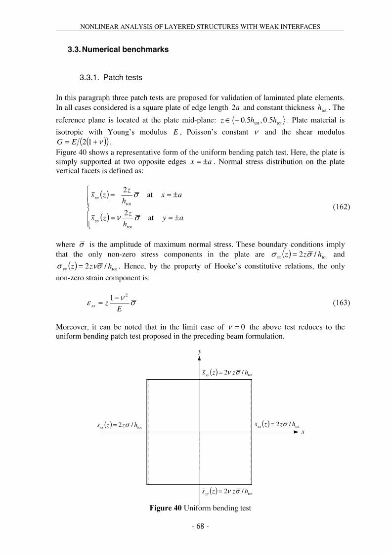
NONLINEAR ANALYSIS OF LAYERED STRUCTURES WITH WEAK INTERFACES
- 68 -
3.3. Numerical benchmarks
3.3.1. Patch tests In this paragraph three patch tests are proposed for validation of laminated plate elements. In all cases considered is a square plate of edge length a2 and constant thickness toth . The
reference plane is located at the plate mid-plane: tottot 5.0,5.0 hhz −∈ . Plate material is
isotropic with Young’s modulus E , Poisson’s constant ν and the shear modulus ( )( )ν+= 12EG .
Figure 40 shows a representative form of the uniform bending patch test. Here, the plate is simply supported at two opposite edges ax ±= . Normal stress distribution on the plate vertical facets is defined as:
)162(
( )
( )⎪⎪⎩
⎪⎪⎨
⎧
±==
±==
ayh
zzs
axh
zzs
yy
xx
at2
at2
tot
tot
σν
σ
where σ is the amplitude of maximum normal stress. These boundary conditions imply that the only non-zero stress components in the plate are ( ) tot/2 hzzxx σσ = and
( ) tot/2 hzzyy σνσ = . Hence, by the property of Hooke’s constitutive relations, the only
non-zero strain component is:
)163( σνεE
zxx
21−=
Moreover, it can be noted that in the limit case of 0=ν the above test reduces to the uniform bending patch test proposed in the preceding beam formulation.
( ) tot/2 hzzsyy σν=
( ) tot/2 hzzsyy σν=
( ) tot/2 hzzsxx σ=
y
( ) tot/2 hzzsxx σ=x
Figure 40 Uniform bending test

NONLINEAR ANALYSIS OF LAYERED STRUCTURES WITH WEAK INTERFACES
- 69 -
A representative form of uniform shear patch test is shown in Figure 41. The plate is again simply supported at two opposite edges ax ±= . The uniform shearing pressure applied at its top and bottom is defined as:
)164( τ=−= BOTTOPxx qq
This implies that the only non-zero stress component in the plate is ττ =xz .
x
y
TOPxq
BOTxq
Figure 41 Uniform shear test
Figure 42 shows the uniform twist patch test. Here the plate is simply supported at three corners. The twisting stress applied at vertical facets of the plate is:
)165(
( )
( )⎪⎪⎩
⎪⎪⎨
⎧
±==
±==
ayh
zzt
axh
zzt
yx
xy
at2
at2
tot
tot
τ
τ
These boundary conditions result in uniform twisting of the plate ( ) tot/2 hzzxy ττ = , where
τ is the amplitude of maximum twisting stress. It is noteworthy that in sharp contrast to the classical form of the twist patch test, e.g. [57], the above formulation is not constrained to the thin plate limit.

NONLINEAR ANALYSIS OF LAYERED STRUCTURES WITH WEAK INTERFACES
- 70 -
x
y
( ) tot/2 hzztxy τ=
0=w 0=w
0=w
( ) tot/2 hzztxy τ=
( ) tot/2 hzztyx τ=
( ) tot/2 hzztyx τ=
Figure 42 Uniform twist test
In order to satisfy the above tests, finite element results should return the imposed uniform stress distributions irrespectively of transverse and planar discretization. For the proposed FE implementation this is achieved only for uniform bending and twisting tests. The uniform shear test is passed for rectangular element meshes. However, when element topology is non-rectangular, the Bathe-Dvorkin approach is insufficient to alleviate the shear locking and element stress field is perturbed. This effect is here assessed by considering a patch of elements proposed in [55]. Figure 43 recalls the details of element mesh and material properties.
x
y
( )5,5
2
−−
( )5,5
7
( )5,5
8
−
( )5,5
1
−
( )2,1
3
− ( )2,3
5
( )2,3
6
−( )3,3
4
−−
0.1
3.0
101.2
tot
6
===
h
E
ν
Figure 43 Element patch for uniform shear test
Table X resumes finite element results obtained with uniform two-layer discretization and uniform isotropic interface stiffness tothGk = . It is worth noting that the average values
of membrane stresses correspond exactly to the expected values. This is verified to be equally true at the element level. In contrast, element transverse shear stress evaluation

NONLINEAR ANALYSIS OF LAYERED STRUCTURES WITH WEAK INTERFACES
- 71 -
remains poor. For example, in element established by nodes 2-8-6-4 average shear stress error is –21.3%. Thus, it can be concluded that the proposed FE implementation is not reliable for analysis of shear-sensitive problems with non-rectangular element meshes.
Table X Uniform shear patch test results (entire plate)
stress patch test FE FE error max 1.000 1.482 48.2 %
xzτ min 1.000 0.690 – 31.0% max 0.000 0.243 -
yzτ min 0.000 – 0.200 - max 1.000 1.444 44.4 %
xf min 1.000 0.481 – 51.9 % max 0.000 1.506 -
yf min 0.000 – 1.202 - max 0.000 1.999 -
xyτ min 0.000 – 1.999 - max 0.000 2.500 -
xxσ min 0.000 – 2.500 - max 0.000 4.511 -
yyσ min 0.000 – 4.511 -
3.3.2. Pagano test The developed FE formulation is validated here using the elasticity solutions obtained by Pagano [58]. Considered here is a rectangular plate tot3 haa ×× . The plate consists of three
layers of equal thickness. The lamination scheme is (0/90/0) and the material properties are identical to those used in the preceding Pagano test (paragraph 3.3.2). Hard simple supports are assumed along all plate edges:
)166( ayw
uax
w
v3,0at
0
0and,0at
0
0=
⎩⎨⎧
==
=⎩⎨⎧
==
Transverse load applied at the plate top is defined as:
)167( ( ) ⎟⎠⎞
⎜⎝⎛
⎟⎠⎞
⎜⎝⎛=
a
y
a
xqyxqz 3
sinsin, 0
ππ
where 0q is the load amplitude.
Table XI compares the elasticity and the FE results for several aspect ratios tothaS = . FE
results are obtained with uniform 1010× mesh per quarter of the plate and three layer discretization. The thin plate ( )100=S results are given to asses the error associated with the FE discretization. It can be observed that with decreasing S , the stress distributions obtained from the elasticity solution become significantly non-symmetric in respect to plate mid-plane. This effect is entirely due to transverse compressibility of the layers. Hence, it is not reproduced by present approach. The tabulated results are normalized using the following relations ( )yxi ,= :

NONLINEAR ANALYSIS OF LAYERED STRUCTURES WITH WEAK INTERFACES
- 72 -
)168(
( ) ( )
( ) ( ) ( ) ( )
( ) ( )Sq
zyxzyx
Sq
zyxzyx
Sq
zyxzyx
h
zzyxw
Shq
Eyxw
iziz
xyxy
iiii
TT
0
20
20
tot4
tot0
,,,,
,,,,;
,,,,
;,100
,
ττ
ττσσ
=
==
==
Table XI Pagano test for plates
( )23
2 , aa
w ( )tot2
12
32 ,, haa
xx
±σ
( )tot61
23
2 ,, haa
yy
±
σ ( )tot2
1,0,0 h
xy
±
τ ( )0,,0 2
3a
xzτ ( )0,0,2
a
yzτ
elasticity 4=S
2.820 1.14 –1.10
0.109 –0.119
–0.0269 0.0281
0.351 0.0334
FE 4=S
2.738 ±0.96 ±0.104 ±0.0257 0.350 0.0307
elasticity 10=S
0.919 0.726 –0.725
0.0418 –0.0435
–0.0120 0.0123
0.420 0.0152
FE 10=S
0.899 ±0.687 ±0.0395 ±0.0116 0.418 0.0146
elasticity 100=S
0.508 ±0.624 ±0.0253 ±0.0083 0.439 0.0108
FE 100=S
0.505 ±0.613 ±0.0243 ±0.0082 0.437 0.0108
Figure 44 shows a representative FE transverse shear stress distribution obtained with the post processing technique introduced earlier for the beam formulation. Also in this case satisfactory agreement with the elasticity solution is obtained.
-0.5
-0.25
0
0.25
0.5
0.0 0.1 0.2 0.3 0.4τ xz
z
layer
interface
Figure 44 Transverse shear stress distribution ( ) 4;,,0 23 =Sza
xzτ
As indicated in 3.2.4, present formulation requires special attention to the simple support. Table XII compares FE results obtained with two types of this boundary condition. In the first case layer rotations about normal to supported edges are suppressed and in the other
( )( )( )( ) 23.0at390.0,,0max
27.0at387.0,,0max
23FE
23elasticity
==
==
zz
zz
axz
z
axz
z
τ
τ

NONLINEAR ANALYSIS OF LAYERED STRUCTURES WITH WEAK INTERFACES
- 73 -
they are left free. As further evidenced in Figure 45 and Figure 46, there is a significant difference in stress distributions near the boundary conditions.
Table XII Pagano test for plate 4=S , influence of boundary conditions
( )23
2 , aa
w ( )tot2
12
32 ,, haa
xx
±σ
( )tot61
23
2 ,, haa
yy
±
σ ( )tot2
1,0,0 h
xy
±
τ ( )0,,0 2
3a
xzτ ( )0,0,2
a
yzτ
FE – rotations suppressed
2.738 ±0.96 ±0.104 ±0.0257 0.350 0.0307
FE – rotations allowed
2.751 ±0.96 ±0.104 ±0.0061 0.353 0.0301
-0.5
-0.25
0
0.25
0.5
-0.03 -0.02 -0.01 0.00 0.01 0.02 0.03τ xy (0,0,z )
z
ROTATIONS SUPPRESSED
ROTATIONS ALLOWED
Figure 45 Twisting stress distribution for two types of boundary condition, 4=S
-0.5
-0.25
0
0.25
0.5
-0.0010 -0.0005 0.0000 0.0005 0.0010σ xx (0,0,z )
z
ROTATIONS SUPPRESSED
ROTATIONS ALLOWED
Figure 46 Normal stress distribution for two types of boundary conditions, 4=S
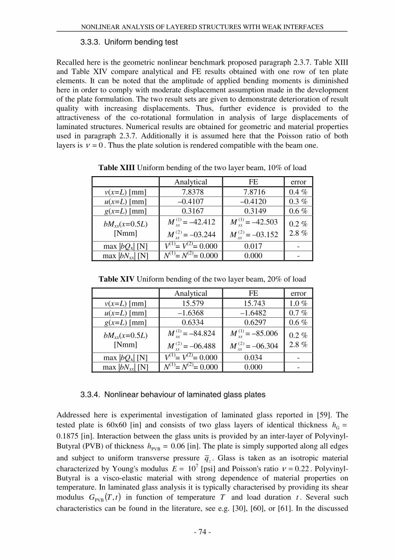
NONLINEAR ANALYSIS OF LAYERED STRUCTURES WITH WEAK INTERFACES
- 74 -
3.3.3. Uniform bending test Recalled here is the geometric nonlinear benchmark proposed paragraph 2.3.7. Table XIII and Table XIV compare analytical and FE results obtained with one row of ten plate elements. It can be noted that the amplitude of applied bending moments is diminished here in order to comply with moderate displacement assumption made in the development of the plate formulation. The two result sets are given to demonstrate deterioration of result quality with increasing displacements. Thus, further evidence is provided to the attractiveness of the co-rotational formulation in analysis of large displacements of laminated structures. Numerical results are obtained for geometric and material properties used in paragraph 2.3.7. Additionally it is assumed here that the Poisson ratio of both layers is 0=ν . Thus the plate solution is rendered compatible with the beam one.
Table XIII Uniform bending of the two layer beam, 10% of load
Analytical FE error v(x=L) [mm] 7.8378 7.8716 0.4 % u(x=L) [mm] –0.4107 –0.4120 0.3 % g(x=L) [mm] 0.3167 0.3149 0.6 %
bMxx(x=0.5L) [Nmm]
)1(xxM = –42.412
)2(xxM = –03.244
)1(xxM = –42.503
)2(xxM = –03.152
0.2 % 2.8 %
max |bQx| [N] V(1)= V(2)= 0.000 0.017 - max |bNxx| [N] N(1)= N(2)= 0.000 0.000 -
Table XIV Uniform bending of the two layer beam, 20% of load
Analytical FE error v(x=L) [mm] 15.579 15.743 1.0 % u(x=L) [mm] –1.6368 –1.6482 0.7 % g(x=L) [mm] 0.6334 0.6297 0.6 %
bMxx(x=0.5L) [Nmm]
)1(xxM = –84.824
)2(xxM = –06.488
)1(xxM = –85.006
)2(xxM = –06.304
0.2 % 2.8 %
max |bQx| [N] V(1)= V(2)= 0.000 0.034 - max |bNxx| [N] N(1)= N(2)= 0.000 0.000 -
3.3.4. Nonlinear behaviour of laminated glass plates Addressed here is experimental investigation of laminated glass reported in [59]. The tested plate is 60x60 [in] and consists of two glass layers of identical thickness =Gh
0.1875 [in]. Interaction between the glass units is provided by an inter-layer of Polyvinyl-Butyral (PVB) of thickness =PVBh 0.06 [in]. The plate is simply supported along all edges
and subject to uniform transverse pressure zq . Glass is taken as an isotropic material characterized by Young's modulus =E 107 [psi] and Poisson's ratio 22.0=ν . Polyvinyl-Butyral is a visco-elastic material with strong dependence of material properties on temperature. In laminated glass analysis it is typically characterised by providing its shear modulus ( )tTG ,PVB in function of temperature T and load duration t . Several such
characteristics can be found in the literature, see e.g. [30], [60], or [61]. In the discussed

NONLINEAR ANALYSIS OF LAYERED STRUCTURES WITH WEAK INTERFACES
- 75 -
experiment the maximum load was incrementally reached in s][60exp =t and the recorded
temperatures were [ ]F80,70 00exp ∈T . However, specific material properties of the PVB
inter-layer are not provided. Instead, it is evidenced that PVB behaviour can be satisfactorily approximated as an elastic one. Using the model adopted in [59] the optimum value of the effective PVB shear modulus was declared to be =PVBG 100 [psi]. As
indicated in Figure 47, this estimation provides a reasonable approximation of the experiment also in present approach, where a mesh of 10x10 elements is used for a quarter of the plate. However, a better fit is attained for =PVBG 146 [psi]. The discrepancy
between the two approaches is due to the finite thickness of the PVB inter-layer (13.8% of the total plate thickness). In present formulation the inter-layer is treated as an interface; thus its thickness is neglected. On the other hand, the development adopted in [59] uses the approach proposed for analysis of sandwich plates with soft core (accounting for finite thickness of the core).
0
0.2
0.4
0.6
0.8
1
0 0.2 0.4 0.6 0.8 1q z [psi]
EXPERIMENT
g=146psi
FE GPVBFE G PVB=100 [psi]
FE G PVB=146 [psi]
cent
ral d
efle
ctio
n [m
m]
Figure 47 Nonlinear response of laminated glass unit, experiment vs. FE
A noteworthy fact here is significant increase of laminated plate stiffness due to the use of relatively soft PVB inter-layer. This can be deduced from Figure 49 where plate response is compared with the limit cases of full layer interaction ∞→PVBG and lack of layer
interaction 0PVB →G .

NONLINEAR ANALYSIS OF LAYERED STRUCTURES WITH WEAK INTERFACES
- 76 -
0
0.2
0.4
0.6
0.8
1
0 0.2 0.4 0.6 0.8 1q z [psi]
g=146psi
FE NO INTERACTION
FE FULL INTERACTION
FE G PVB=146 [psi]
cent
ral d
efle
ctio
n [m
m]
Figure 48 Influence of PVB inter-layer on laminated glass stiffness
3.3.5. Laminated glass buckling Addressed here is experimental investigation of laminated glass buckling reported in [62]. Figure 49 shows schematic representation of the experiment. A square plate of edge length
]mm[1000=a is simply supported along all edges and loaded in its plane by imposing
uniform lateral displacement v . The plate consists of two glass layers of thickness Gh = 8
[mm] and a thin inter-layer of Polyvinyl-Butyral of thickness PVBh = 1.52 [mm].
x
y
a
v
v
a
Figure 49 Laminated glass buckling, schematic representation

NONLINEAR ANALYSIS OF LAYERED STRUCTURES WITH WEAK INTERFACES
- 77 -
Figure 50 shows details of plate mounting at y=±0.5a. It can be deduced that fastening metallic clamps gives rise to friction between glass sheets constituting the plate, washers and clamps. This friction restricts relative movement of the two glass sheets. Thus, present (Finite Element) model uses essential boundary conditions to suppress interface slips (gx and gy) at y=±0.5a. On the other hand, both interface slips are left free at x=±0.5a, where the experimental setup does not restrict slippage.
Figure 50 Detailed view of experimental setup at y=±0.5a
Three experimental results are reported in [62]. The experiments were conducted at the average temperature of [ ]C200
exp ≈T and the average time needed to reach the ultimate
load was s][5000exp ≈t . Thus, following the discussion given in [62], the effective (linear,
elastic) stiffness of the PVB interlayer can be estimated to be PVBG = 0.8 [MPa]. Glass
Young’s modulus is taken as =E 7 104 [MPa] and Poisson’s ratio is 23.0=ν . Figure 51 compares experimental and present (Finite Element) results obtained with uniform 10x10 element mesh per quarter of the plate. N is the total compressive force (integrated along edge y=+0.5a). Numerical results are obtained taking the reference plane at =)1(
eccz 3 [mm] (1 [mm] away from the plate mid-plane). This location is chosen to match
the laminate response in early stage of loading.
0
100
200
300
400
500
600
700
0 2 4 6 8 10 12 14 16w (0,0) [mm]
N [
kN]
Experiment 1
Experiment 2
Experiment 3
FE model
Figure 51 Laminated glass buckling, comparison of experimental and FE results

NONLINEAR ANALYSIS OF LAYERED STRUCTURES WITH WEAK INTERFACES
- 78 -
3.4. Summary for plate formulation In the above, the analytical and the finite element formulation is provided for geometric nonlinear analysis of laminated plates subject to moderately large displacements (in the von Kármán sense). The development is performed assuming Reissner-Mindlin kinematics at each layer and moderate slip at layer interfaces. No transverse separation is allowed. Analogously to the preceding beam development using interface slips as independent variables allows obtaining robust FE formulation for laminated plates. However, the approach is shown unsuitable for the extension to the shallow shell formulation. As evidenced in numerical benchmarks, the proposed model is capable of representing complex stress distributions expected in laminated plate structures with large transverse anisotropy. It is also shown to provide reliable description to a number of geometric nonlinear effects. However, the adopted FE implementation does not provide satisfactory solution to the shear locking for non-rectangular element configurations. Thus, a suitable solution to this problem needs yet to be identified.

NONLINEAR ANALYSIS OF LAYERED STRUCTURES WITH WEAK INTERFACES
- 79 -
4. Shallow shells Laminated shell is assumed here to undergo arbitrary large displacements, moderate interface slips and be subject to small layer strains. Thus, allowing for shallow initial configuration, the co-rotational FE formulation can be used to approximate shell behaviour with elements having flat reference surface, small initial curvature, and subject to moderate deforming displacements (in the von Kármán sense). Therefore, the purpose of present development is to extend the preceding plate formulation to accommodate the required features.
4.1. Theoretical development
4.1.1. Kinematic relations Laminated plate kinematic field developed in paragraph 3.1.1 makes use of simplifying assumptions preventing its consistent 3D rotation. Hence, it is not well suited for the intended FE shell formulation. The encountered problems can be cast here into two categories. In the first one, no )(lay
zθ rotations appear in description of layer displacement field. This problem received substantial amount of interest in single-layer formulations. The successful approaches can be sub-divided into two main trends. Representative of the first one is the pioneering work of Allman [63] where vertex rotations zθ are used to enhance FE kinematic field. Despite additional problems with numerical locking and zero energy mode control (e.g. [64]), this method gained substantial popularity due to its relative simplicity. In more recent works, e.g. [65] and [66], drilling rotations zθ are introduced as independent kinematic field. Here however, the use of mixed principles is necessary to enforce the strain and the stress tensor symmetry. It can be shown that any of the aforementioned approaches can be applied at the layer level of present (layer-wise) development. However, for the sake of simplicity Allman`s approach is assumed here and the vertex rotations )(lay
zθ are introduced only at the stage of the FE development. Another difficulty with 3D rotations is associated with the use of interface slips as independent variables. These quantities constitute a 2D vector field. Therefore, transformation of this field is rather awkward in case of 3D rotation of the reference frame. To circumvent this problem present development uses the following vector description of interface displacement:
)169( ( ) ( ) ( ) ( )[ ]yxwyxvyxuyx intintintint ,,,,,, )()()(T)( ΔΔΔ=Δ
where ( )yxu int ,)(Δ , ( )yxv int ,)(Δ and ( )yxw int ,)(Δ are projections of the total interface
displacement ( )yxint ,)(Δ on relevant axes of the adopted reference frame. Hence, using these quantities as independent variables provides appropriate dimension and straightforward 3D rotation of the interface displacement field. However, it does not exclude the possibility of layer transverse separation/overlapping. Figure 52 shows a representative vector )(intΔ and its projections on the reference system axes. Assuming moderate interface slips and small layer strains allows local approximation of the deformed interface surface as a plane (shaded area in Figure 52). In this case, vector
)(intΔ can be restricted to represent only interface slippage by stating:

NONLINEAR ANALYSIS OF LAYERED STRUCTURES WITH WEAK INTERFACES
- 80 -
)170( ( ) ( ) ( )[ ] ( ) ( )[ ]yxyxvyxyxuyxw inty
intintx
intint ,tg,,tg,, )()()()()( αα Δ+Δ=Δ
where ( )yxint
j ,)(α are interface rotation angles defined as:
)171( ( )( )
( )⎪⎪⎩
⎪⎪⎨
⎧
⎥⎦
⎤⎢⎣
⎡∂
−=∂
⎥⎦
⎤⎢⎣
⎡∂
=∂
=
−−−−
knownif,,
arctg
knownif,,
arctg
,)(
)(21)()(
)1()1(
21)1()1(
)(
intintintint
intintintint
intj
wj
hzyxw
wj
hzyxw
yxα
where ( ))()( ,, laylay zyxw is layer transverse displacement field (note the analogy to the relation (4) of the laminated beam development).
)(intwΔ
z
y
x
z||
y||
x||
)( intvΔ
)(intuΔ
)(intxg
)(intyg
)(intxα
)(intyα
)(intΔ
Figure 52 Vector representation of interface displacement
Thus, assuming that )1( −intw is known:
)172(
( ) ( ) ( )
( ) ( )y
hzyxwyxv
x
hzyxwyxuyxw
intintintint
intintintintint
∂=∂
Δ+
+∂
=∂Δ=Δ
−−−
−−−
)1(21)1()1(
)(
)1(21)1()1(
)()(
,,,
,,,,
or if )(intw is known:
)173(
( ) ( ) ( )
( ) ( )y
hzyxwyxv
x
hzyxwyxuyxw
intintintint
intintintintint
∂−=∂
Δ+
+∂
−=∂Δ=Δ
)(21)()(
)(
)(21)()(
)()(
,,,
,,,,
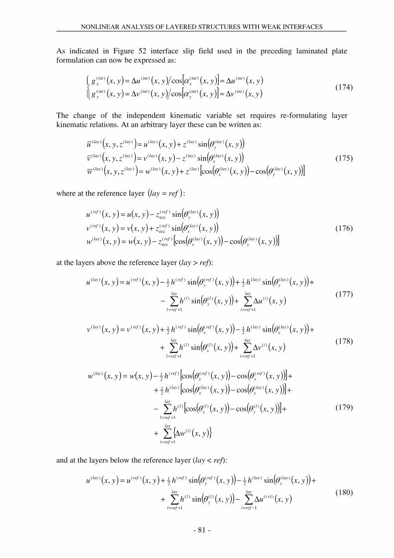
NONLINEAR ANALYSIS OF LAYERED STRUCTURES WITH WEAK INTERFACES
- 81 -
As indicated in Figure 52 interface slip field used in the preceding laminated plate formulation can now be expressed as:
)174( ( ) ( ) ( )[ ] ( )( ) ( ) ( )[ ] ( )⎪⎩
⎪⎨⎧
Δ≈Δ=
Δ≈Δ=
yxvyxyxvyxg
yxuyxyxuyxgintint
yintint
y
intintx
intintx
,,cos,,
,,cos,,)()()()(
)()()()(
αα
The change of the independent kinematic variable set requires re-formulating layer kinematic relations. At an arbitrary layer these can be written as:
)175(
( ) ( ) ( )( )( ) ( ) ( )( )( ) ( ) ( )( ) ( )( )[ ]yxyxzyxwzyxw
yxzyxvzyxv
yxzyxuzyxu
layy
layx
laylaylaylay
layx
laylaylaylay
layy
laylaylaylay
,cos,cos,,,
,sin,,,
,sin,,,
)()()()()()(
)()()()()(
)()()()()(
θθθ
θ
−+=
−=
+=
where at the reference layer ( )reflay = :
)176(
( ) ( ) ( )( )( ) ( ) ( )( )( ) ( ) ( )( ) ( )( )[ ]yxyxzyxwyxw
yxzyxvyxv
yxzyxuyxu
layy
layx
reflay
layx
refref
layy
refref
,cos,cos,,
,sin,,
,sin,,
)()()(ecc
)(
)()(ecc
)(
)()(ecc
)(
θθθ
θ
−−=
+=
−=
at the layers above the reference layer (lay > ref):
)177(
( ) ( ) ( )( ) ( )( )( )( ) ( )∑∑
+=+=
Δ+−
++−=lay
refi
ilay
refl
ly
l
layy
layrefy
refreflay
yxuyxh
yxhyxhyxuyxu
1
)(
1
)()(
)()(21)()(
21)()(
,,sin
,sin,sin,,
θ
θθ
)178(
( ) ( ) ( )( ) ( )( )( )( ) ( )∑∑
+=+=
Δ++
+−+=lay
refi
ilay
refl
lx
l
layx
layrefx
refreflay
yxvyxh
yxhyxhyxvyxv
1
)(
1
)()(
)()(21)()(
21)()(
,,sin
,sin,sin,,
θ
θθ
)179(
( ) ( ) ( )( ) ( )( )[ ]( )( ) ( )( )[ ]( )( ) ( )( )[ ]
( ) ∑
∑
+=
+=
Δ+
+−−
+−+
+−−=
lay
refi
i
lay
refl
ly
lx
l
layy
layx
lay
refy
refx
reflay
yxw
yxyxh
yxyxh
yxyxhyxwyxw
1
)(
1
)()()(
)()()(21
)()()(21)(
,
,cos,cos
,cos,cos
,cos,cos,,
θθ
θθ
θθ
and at the layers below the reference layer (lay < ref):
)180(
( ) ( ) ( )( ) ( )( )( )( ) ( )∑∑
−=
+
+=
Δ−+
+−+=lay
refi
ilay
refl
ly
l
layy
layrefy
refreflay
yxuyxh
yxhyxhyxuyxu
1
)1(
1
)()(
)()(21)()(
21)()(
,,sin
,sin,sin,,
θ
θθ

NONLINEAR ANALYSIS OF LAYERED STRUCTURES WITH WEAK INTERFACES
- 82 -
)181(
( ) ( ) ( )( ) ( )( )( )( ) ( )∑∑
−=
+
+=
Δ−−
++−=lay
refi
ilay
refl
lx
l
layx
layrefx
refreflay
yxvyxh
yxhyxhyxvyxv
1
)1(
1
)()(
)()(21)()(
21)()(
,,sin
,sin,sin,,
θ
θθ
)182(
( ) ( ) ( )( ) ( )( )[ ]( )( ) ( )( )[ ]( )( ) ( )( )[ ]
( ) ∑
∑
−=
+
+=
Δ−
+−+
+−−
+−+=
lay
refi
i
lay
refl
ly
lx
l
layy
layx
lay
refy
refx
reflay
yxw
yxyxh
yxyxh
yxyxhyxwyxw
1
)1(
1
)()()(
)()()(21
)()()(21)(
,
,cos,cos
,cos,cos
,cos,cos,,
θθ
θθ
θθ
Moderate rotations expected in the co-rotational FE formulation allow simplifying the above relations by expanding trigonometric functions into Taylor series and truncating higher order terms. In such case layer kinematic relations can be written in the following linear form:
)183(
( ) ( ) ( )( ) ( ) ( )( ) ( )yxwzyxw
yxzyxvzyxv
yxzyxuzyxu
laylaylay
layx
laylaylaylay
layy
laylaylaylay
,,,
,,,,
,,,,
)()()(
)()()()()(
)()()()()(
≈
−≈
+≈
θ
θ
where at the reference layer (lay = ref):
)184(
( ) ( ) ( )( ) ( ) ( )( ) ( )yxwyxw
yxzyxvyxv
yxzyxuyxu
lay
refx
ref
refy
ref
,,
,,,
,,,
)(
)(ecc
)(
)(ecc
)(
≈
+≈
−≈
θ
θ
at layers above the reference layer (lay > ref):
)185(
( ) ( ) ( ) ( )
( ) ( )
( ) ( ) ( ) ( )
( ) ( )
( ) ( ) ( )yxwyxwyxw
yxvyxh
yxhyxhyxvyxv
yxuyxh
yxhyxhyxuyxu
lay
refi
ilay
lay
refi
ilay
refl
lx
l
layx
layrefx
refreflay
lay
refi
ilay
refl
ly
l
layy
layrefy
refreflay
,,,
,,
,,,,
,,
,,,,
1
)()(
1
)(
1
)()(
)()(21)()(
21)()(
1
)(
1
)()(
)()(21)()(
21)()(
∑
∑∑
∑∑
+=
+=+=
+=+=
Δ+≈
Δ++
+−+≈
Δ+−
++−≈
θ
θθ
θ
θθ
and finally, at the layers below the reference layer (lay < ref):

NONLINEAR ANALYSIS OF LAYERED STRUCTURES WITH WEAK INTERFACES
- 83 -
)186(
( ) ( ) ( ) ( )
( ) ( )
( ) ( ) ( ) ( )
( ) ( )
( ) ( ) ( )∑
∑∑
∑∑
−=
+
−=
+
−=
−=
+
−=
Δ−≈
Δ−−
++−≈
Δ−+
+−+≈
lay
refi
ilay
lay
refi
ilay
refl
lx
l
layx
layrefx
refreflay
lay
refi
ilay
refl
ly
l
layy
layrefy
refreflay
yxwyxwyxw
yxvyxh
yxhyxhyxvyxv
yxuyxh
yxhyxhyxuyxu
1
)1()(
1
)1(
1
)()(
)()(21)()(
21)()(
1
)1(
1
)()(
)()(21)()(
21)()(
,,,
,,
,,,,
,,
,,,,
θ
θθ
θ
θθ
From (170) it can be concluded that ( )yxw int ,)(Δ is significantly smaller than ( )yxw , .
Thus, the above relations could be further simplified leading to constant transverse displacement across laminate thickness. This simplification was shown to be the source of some minor problems in the laminated beam formulation. Thus, leaving ( )yxw int ,)(Δ in
(185) and (186) gives present approach the potential to avoid these problems. It can also be noted that neglecting influence of ( )yxw int ,)(Δ and using (174) to replace
( )yxu int ,)(Δ and ( )yxv int ,)(Δ with interface slips, the form of linearized kinematic relations
is identical to the ones formulated for analysis of laminated plates.
4.1.2. Geometric relations Layer-wise strain field of the von Kármán type can now be written in the following form:
)187( )(M
)(vK
)(0
)( laylaylaylay εεεε ++=
where the linear strain field )(
0layε is defined as (note the use of deforming displacements
and moving reference frame):
)188(
⎥⎥⎥⎥⎥⎥⎥⎥⎥⎥⎥⎥
⎦
⎤
⎢⎢⎢⎢⎢⎢⎢⎢⎢⎢⎢⎢
⎣
⎡
−∂
∂
+∂
∂
⎟⎟⎠
⎞⎜⎜⎝
⎛
∂∂−
∂∂
+∂
∂+∂
∂∂
∂−∂
∂∂
∂+
∂∂
=
)(*)(*
)(*)(*
)(*)(*)(
)(*)(*
)(*)(
)(*
)*()(
)*(
)(0
'
'
'''
''
''
'
''
'
layx
lay
layy
lay
layx
layylay
laylay
layxlay
lay
layylay
lay
lay
y
wx
w
xyz
x
v
y
u
yz
y
vx
zx
u
θ
θ
θθ
θ
θ
ε
Geometric nonlinear part of von Kármán strains is:

NONLINEAR ANALYSIS OF LAYERED STRUCTURES WITH WEAK INTERFACES
- 84 -
)189(
⎥⎥⎥⎥⎥⎥⎥⎥⎥⎥⎥
⎦
⎤
⎢⎢⎢⎢⎢⎢⎢⎢⎢⎢⎢
⎣
⎡
∂∂
∂∂
⎟⎟⎠
⎞⎜⎜⎝
⎛
∂∂
⎟⎟⎠
⎞⎜⎜⎝
⎛
∂∂
=
0
0''
'2
1
'2
1
)(*)(*
2)(*
2)(*
)(vK
y
w
x
w
y
w
x
w
laylay
lay
lay
layε
Using Marguerre's approach to account for initial curvature of the reference surface, vector
)(Mlayε is:
)190(
⎥⎥⎥⎥⎥⎥⎥⎥⎥⎥
⎦
⎤
⎢⎢⎢⎢⎢⎢⎢⎢⎢⎢
⎣
⎡
∂∂
∂∂+
∂∂
∂∂
∂∂
∂∂
∂∂
∂∂
=
0
0''''
''
''
)(*
00
)(*
0
)(*
0
)*(
)(M
y
w
x
w
y
w
x
wy
w
y
wx
w
x
w
laylay
lay
lay
layε
4.1.3. Constitutive relations Constitutive relations used in present formulation are identical as the ones proposed for the laminated plate development (see paragraph 3.1.3).
4.1.4. Equilibrium relations Present approach employs Nlay5 independent kinematic variables. Thus, the same number of equilibrium relations needs to be provided. 14 +Nlay of them are the equilibrium relations developed in paragraph 3.1.4 for laminated plate formulation. The remaining
1−Nlay relations are obtained by constraining interface displacement field to represent only layer slippage. This is obtained by writing equation (170) at each interface. In the perspective of FE development it is particularly convenient to do so by using relations (172) or (173). Regarding the weak form of equilibrium, only the expression for virtual work of internal forces is here changed in respect to the form provided for laminated plates. In present development it can be written as:
)191( ( ) ( )∑∫∑ ∫==
++=Nlay
int A
intintintintintNlay
lay Ω
laylaylay AccΩWlay 2
)()(C
)()(T)(
1
)()(T)( dd)(
λδδδδ fgσεint
where equations constraining interface displacement field are incorporated through variable ( )yxc int ,)( . If )1( −intw is known then:

NONLINEAR ANALYSIS OF LAYERED STRUCTURES WITH WEAK INTERFACES
- 85 -
)192( ( ) ( ) ( ) ( )
( ) ( )y
hzyxwyxv
x
hzyxwyxuyxwyxc
intintintint
intintintintintint
∂=∂Δ−
+∂
=∂Δ−Δ=
−−−
−−−
)1(21)1()1(
)(
)1(21)1()1(
)()()(
,,,
,,,,,
or if )(intw is known then:
)193( ( ) ( ) ( ) ( )
( ) ( )y
hzyxwyxv
x
hzyxwyxuyxwyxc
intintintint
intintintintintint
∂−=∂Δ−
+∂
−=∂Δ−Δ=
)(21)()(
)(
)(21)()(
)()()(
,,,
,,,,,
It should be noted here that the variable ( )yxc int ,)( contains linear, as well as, geometric
nonlinear terms. Thus, it can be concluded that incorporating it in the FE matrix formulation results in substantial increase of computational effort necessary to establish consistent tangent stiffness matrix. This effort cannot be diminished by neglecting the geometric nonlinear terms in (192) and (193), as these terms can be as large as the linear term. Additionally, it can be observed that the unit of the penalty parameter )(
Cintλ is [N/m3].
Thus, it is identical as the unit of interface stiffness )(intk .

NONLINEAR ANALYSIS OF LAYERED STRUCTURES WITH WEAK INTERFACES
- 86 -
4.2. Finite element development
4.2.1. Co-rotational finite element formulation Detailed co-rotational shallow laminated shell matrix formulation can be straightforwardly obtained using elements of the preceding beam and plate formulations. Thus, discussed here are only selected components of this development. The form of consistent tangent stiffness matrix at the element level can now be written as:
)194( ( ) ( ) ( )*** dKdKdK σ+=TAN
First, it should be noted that only deforming displacements *d are used in (194). Second, the vector of element DOF’s is here substantially larger than in case of laminated plate element. For example, at a representative node m the vector of nodal DOF’s is now:
)195( [ ])()()()()()()1()1()1(T ,,,,,...,,,,,, Nlaymz
Nlaymy
Nlaymx
Nlaym
Nlaym
Nlaymmzmymxmmmm wvuwvu θθθθθθ ΔΔΔ=d
Thus, it contains Nlay6 components instead of 14 +Nlay used at laminated plate nodes.
Matrix ( )dK is now defined as:
)196(
( ) ( ) ( ) ( ) ( )( ) ( )
∑ ∫
∑ ∫
=
= Ω
⎪⎭
⎪⎬⎫
⎪⎩
⎪⎨⎧
+
++
=
Nlay
int Aintintint
intg
intintg
Nlay
lay
laylaylaylaylaylay
Ayxyx
yxyx
Ωzyxzyxlay
2 )(C
)(C
T)(C
)()(T)(
1
)()()()()(T)(
d,,,,
,,
d,,,,,,)(
dBdB
NkN
dBDdBdK
λ
where:
)197( ( ) ( ) ( ) ( )
( )dB
dBBBdB
,,
,,,,,,,,)(
vK
0)(
M)(
A)()(
0)()(
yx
yxyxzyxzyxlay
laylaylaylaylaylay
+
+++=
)198(
( )
( )
( )
( )⎪⎪⎪⎪⎪
⎩
⎪⎪⎪⎪⎪
⎨
⎧
∂∂=
∂∂=
∂∂=
∂∂=
dε
dB
dε
dB
dε
B
dε
B
)(vK)(
vK
)(M
0)(
M
)(A)(
A
)(0)()(
0
,,
,,
,
,,
laylay
laylay
laylay
laylaylay
yx
yx
yx
zyx
In the above matrix ( ))()(
0 ,, laylay zyxB refers to geometric linear strains defined in (188),
( )0)(
M ,, dB yxlay refers to geometric linear strain field associated with given initial curvature
0d (relation (190)), ( )dB ,,)(vK yxlay refers to geometric nonlinear strains defined in (189)

NONLINEAR ANALYSIS OF LAYERED STRUCTURES WITH WEAK INTERFACES
- 87 -
and ( )yxlay ,)(AB refers to layer-wise strains ( ))()(
A ,, laymz
lay yx θε appearing as a result of
enriching element kinematic field with the vertex rotations. In Allman’s approach these strains are in general geometric linear relations dependent on adopted element topology. Thus, particular form of these is not yet defined here. In (196) vector ( )dB ,,)(
C yxint represents nonlinear interface constraint and is defined as:
)199( ( )d
dB∂
∂=
)()(
C ,,int
int cyx
The initial stress matrix ( )dKσ is now defined as:
)200(
( ) ( ) ( )
( ) ( )∑ ∫
∑ ∫
=
= Ω
⎪⎭
⎪⎬⎫
⎪⎩
⎪⎨⎧
∂∂+
+⎪⎭
⎪⎬⎫
⎪⎩
⎪⎨⎧
∂∂=
Nlay
int A
intintint
Nlay
lay
laylaylaylay
Ayxcyx
Ωzyxyx
lay
2
)()(C
T)(C
1
)()()(
T)(vK
d,,,,
d,,,,,
)(
dd
dB
dσd
dBdK
λ
σ
4.2.2. On finite element implementation Briefly discussed here is an attempt to implement the above formulation in the form of 4 node quadrilateral used in the preceding plate development. For such element topology the vertex rotations can be independently incorporated at each layer following the development presented in [64]. In this case, standard bi-linear interpolation of layer kinematic field is enriched by quadratic interpolation associated with vertex rotations. Obviously, this leads to membrane locking due to incompatibility of layer strain interpolation. In single-layer approaches it is typically alleviated by using reduced 2x2 Gaussian integration scheme and adding stabilization matrices to assure under-integrated element performance. However, in multi-layer case this is insufficient and membrane locking persists. This is due to the incompatibility of layer and interface displacement field interpolation. This implies that an interface of non-zero stiffness is unable to consistently transmit inter-laminar forces. Taking into consideration the co-rotational character of present formulation, the most advantageous solution to this problem seems to be including hierarchic modes to selectively enrich interface interpolation. This however, needs yet to be investigated.

NONLINEAR ANALYSIS OF LAYERED STRUCTURES WITH WEAK INTERFACES
- 88 -
4.3. Summary for shallow shell formulation Presented in the above paragraphs are some general lines for the FE co-rotational analysis of shallow laminated shells subject to arbitrary large displacements, moderate interface slips and small layer strains. Rigorous development of theoretical basis (in particular layer-wise kinematics) allows expecting fine performance of elements based on the proposed formulation. However, FE implementation allowing satisfactory suppression of all numerical locking needs yet to be studied in detail. It should also be noted that the versatility of laminated shell formulation is obtained at the expense of substantial increase of computational demands in respect to the preceding plate development. This observation underlines the usefulness of less resourceful, but computationally efficient, models of laminated beams and plates.
NONLINEAR ANALYSIS OF LAYERED STRUCTURES WITH WEAK INTERFACES
- 89 -
5. Concluding remarks This chapter provides summary of the key observations regarding present work and perspectives of further development. The co-rotational FE formulation is shown to be a simple and efficient mean of geometric nonlinear analysis of laminated structures. The possibility of using linearized kinematic relations and the von Kármán strain measure is particularly advantageous in the analysis of laminates with weak interfaces where the combined complexity of kinematic and geometric relations limits preceding (Total-Lagrangian) developments to the moderate displacement regime. Thus, the co-rotational formulation can be used to substantially extend versatility of some, readily available, models. However, the co-rotational approach requires evaluation of element deforming displacement field, which in turn necessitates rigorous approach to the formulation of laminate kinematics. In present work this is assured by starting the considerations from the assumption of arbitrary large displacements. The additional benefit of such approach is the insight to the linearized model limitations and possibilities of its refinement. For example, it is here observed that neglecting influence of interface slips on layer transverse displacement field allows significant simplifications; but it is also the source of minor stress re-distribution within laminate thickness. Thus, an approach avoiding this effect and maintaining computational robustness is worth pursuing. Another interesting observation can be made regarding the choice of independent variable set used to formulate layer-wise kinematic relations. Employing interface slips as independent variables allows constructing simple and computationally efficient beam and plate models. However, the same approach is shown to be rather cumbersome in shell formulation. This problem is resolved here by changing independent variables used to define interface displacement field. This however, necessitates introducing additional interface constraint equations which reduce computational robustness of the approach. Thus, it is worth investigating alternative possibilities of formulating robust, yet consistent, shell formulation. It can be noted that the form of layer constitutive relations used in present work is identical as in relevant single-layer approaches. As evidenced in the laminated beam development, this allows straightforward extension of present FE formulations to include the variety of material nonlinear models readily available for such single-layer approaches. Underlined here should also be the importance of efficient alleviation of numerical locking. As indicated in laminated plate and shell developments, methods considered satisfactory in single-layer approaches are not necessarily sufficient in multi-layer ones. Particularly important here is alleviation of the shear locking, as the shear stresses govern layer delamination and may in consequence lead to global laminate failure. The above remark allows identifying yet another prospective direction of development. Assuming FSDT at the layer level, present approach does not satisfy the theoretical requirement stating 0C inter-laminar continuity of transverse shear stresses. Thus,
recognizing importance of these stresses, it is worth investigating possibilities of meeting the above requirement. One such opportunity is indicated in the laminated beam approach, where mixed principle is proposed to enhance the formulation with the assumed shear stress distribution.

NONLINEAR ANALYSIS OF LAYERED STRUCTURES WITH WEAK INTERFACES
- 90 -
6. References
[1] Reddy J.N., (1997), Mechanics of Laminated Composite Plates, CRC Press, Inc., Boca Raton
[2] Carrera E., (1997), "C0
z Requirements – Models for the Two Dimensional Analysis of Multilayered Structures", Composite Structures, Vol. 37, pp 373-384
[3] Reddy J.N., (1991), "A Transverse Deformation Theory of Laminated Composite
Plates", Computers and Structures, Vol. 41, pp 821-833
[4] Murakami H., (1986), "Laminated composite plate theory with improved in-plane responses", Journal of Applied Mechanics, Vol. 53, pp 661-666
[5] Averill R.C., Yip Y.Ch., (1996), "Development of Simple Robust Finite Elements
Based on Refined Theories for Thick Laminated Beams", Computers and Structures, Vol. 59, pp 529-546
[6] Noor A.K., Burton W.S., (1989), "Assessment of shear deformation theories for
multilayered composite plates", Applied Mechanics Review, Vol. 41, pp 1-18
[7] Reddy J.N., Robbins D.H., (1994), "Theories and computational models for composite laminates", Applied Mechanics Review, Vol. 47, pp 147-165
[8] Carrera E. (2002), "Theories and finite elements for multilayered, anisotropic,
composite plates and shells", Archives of Computational Methods in Engineering, Vol. 9, pp 87-140
[9] Carrera E., (2000), "A priori vs. a posteriori evaluation of transverse stresses in
multilayered orthotropic plates", Composite Structures, Vol. 48, pp 245-260
[10] Fraternalli F., Reddy J.N., (1993), "A Penalty Model for the Analysis of Laminated Composite Shells", International Journal of Solids and Structures, Vol. 30, pp 3337-3355
[11] Dau F., Polit O., Touratier M., (2004) "An Efficient C1 Finite Element with
Continuity Requirements for Multilayered/Sandwich Shell Structures", Computes and Structures, Vol. 82, pp 1889-1899
[12] Williams T.O., Addessio F.L., (1997), "A General Theory for Laminated Plates
With Delaminations", International Journal of Solids and Structures, Vol. 34, pp 2003-2024
[13] Soldatos K.P., Shu X., (2001), "Modelling of Perfectly and Weakly Bonded
Laminated Plates and Shallow Shells", Composites Science and Technology, Vol. 61, pp 247-260
[14] Reddy J.N., Kuppusamy T., (1984), "A Three-Dimensional Nonlinear Analysis of
Cross-Ply Rectangular Composite Plates", Computers & Structures, Vol. 18, pp 263-272

NONLINEAR ANALYSIS OF LAYERED STRUCTURES WITH WEAK INTERFACES
- 91 -
[15] Zinno R., Barbero E.J., (1995), "Total Lagrangian Formulation for Laminated Composite Plates Analysed by Three-Dimensional Finite Elements with Two-Dimensional Kinematic Constraints", Computers and Structures, Vol. 57, pp 455-466
[16] Pai P.F., Palazotto A., (1995), "Nonlinear Displacement-Based Finite-Element
Analysis of Composite Shells - a New Total Lagrangian Formulation", International Journal of Solids and Structures, Vol. 32, pp 3047-3073
[17] Zielinski A.P., Frey F., (2003), "Nonlinear Weighted Residual Approach:
Application to Laminated Beams", Computers and Structures, Vol. 81, pp 1087-1098
[18] Oven V.A., Burgess I.W., Plank R.J., Wali A.A.A., (1997), "An Analytical Model
for the Analysis of Composite Beams with Partial Interaction", Computers and Structures, Vol. 62, pp 493-504
[19] Saje M., Cas B., Planinc I., (2004), "Non-Linear Finite Element Analysis of
Composite Planar Frames With an Interlayer Slip", Computers and Structures, Vol. 82, pp1901-1912
[20] Girhammar U.A., Gopu V.K.A., (1993), "Composite Beam-Columns with Inter-
layer Slip - Exact Analysis", Journal of Structural Engineering ASCE, Vol. 119, pp 1265-1282
[21] Cheng Z.Q., Howson W.P., Williams F.W., (1997), "Modelling of Weakly
Bonded Laminated Composite Plates at Large Deflections", International Journal of Solids and Structures, Vol. 34, pp 3583-3599
[22] Zhang Y., Wang S., Petersson B., (2003), "Large Deflection Analysis of
Composite Laminates", Journal of Materials Processing Technology, Vol. 138, pp 34-40
[23] Qiu Y., Crissfield M.A., Alfano G., (2001), "An Interface Element Formulation
for the Simulation of Delamination with Buckling", Engineering Fracture Mechanics, Vol. 68, pp 1755-17876
[24] Larsson R., (2004), "A Discontinuous Shell-Interface Element for Delamination
Analysis of Laminated Composite Structures", Computational Methods in Applied Engineering, Vol. 193, pp 3173-3194
[25] Bruno D., Grecko F., Lonetti P., (2005), "A 3D Delamination Modelling
Technique Based on Plate and Interface Theories for Laminated Structures", European Journal of Mechanics A/Solids, Vol. 24, pp 127-149
[26] Dominguez N., Brancherie D., Ibrahimbegović A., (2005), "Prediction of Crack
Pattern Distribution in Reinforced Concrete by Coupling a Strong Discontinuity Model of Concrete Cracking and a Bond-Slip of Reinforcement Model", Engineering Computations, Vol.22, pp 558-582
[27] Zenkert D., (1997), The Handbook of Sandwich Construction, Engineering
Materials Advisory Service Ltd., United Kingdom

NONLINEAR ANALYSIS OF LAYERED STRUCTURES WITH WEAK INTERFACES
- 92 -
[28] Pirazzi C., (2005), "Zur Berechnung von Holzschalen in Brettrippenbauweise mit
Elastischem Verbundquerschnitt", Ph.D. thesis, Ecole Polytechnique Fédérale de Lausanne
[29] Yam L.C.P., Chapman J.C., (1972), "The Inelastic Behaviour of Continuous
Composite Beams of Steel and Concrete" Proceedings of Institution of Civil Engineers, Vol. 53, pp 487-501
[30] Van Duser A., Jagota A., Bennison S.J., (1999), "Analysis of Glass/Polyvinyl
Butyral Laminates Subjected to Uniform Pressure", Journal of Engineering Mechanics, Vol. 125, pp 435-442
[31] Crisfield M.A., Moita G.F., (1996), "A Unified Co-rotational Framework for
Solids, Shells and Beams", International Journal of Solids and Structures, Vol. 33, pp 2969-2992
[32] Marguerre K., (1933), "Zur Theorie der Gekrümmten Platte Großer
Formänderung", Jahrbuch des 1939 der Deutschen Luftfahrforschnung, p. 413
[33] Jetteur P., (1986), “Implicit Integration Algorithm for Elastoplasticity in Plane Stress Analysis”, Engineering Computations, Vol. 3, pp 251-253
[34] Simo J.C., Taylor R.L., (1986) "A Return Mapping Algorithm for Plane Stress
Elastoplasticity", International Journal for Numerical Methods in Engineering, Vol. 22, pp 649-670
[35] Wilkins M.L., (1964), "Calculation of Elasto-Plastic Flow", Methods of
Computational Physics 3”, Academic Press, New York
[36] Murakami H., (1984), "A Laminated Beam Theory with Inter-layer Slip", Journal of Applied Mechanics, Vol. 51, pp 551-559
[37] Girija Vallabhan C.V., Das Y.C., Ramasamudra M., (1992), "Properties of PVB
Inter-Layer Used in Laminated Glass", Journal of Materials in Civil Engineering, Vol. 4, pp 71-77
[38] Hughes T.J.R., (2000), The Finite Element Method - Linear Static and Dynamic
Finite Element Analysis, Dover Publications Inc., Mineola, New York
[39] Kim Y., Davalos J. F., Barbero E.J, (1994), "Composite Beam Element with Layer-Wise Plane Sections", Journal of Engineering Mechanics ASCE, Vol. 120, pp1160-1166
[40] Zienkiewicz O.C., Taylor R.L., (2000), The Finite Element Method, Vol.
1, Butterworth Heinemann, Oxford, pp 370-375
[41] Reissner E., (1984), "On a Certain Mixed Variational Theorem and Proposed Application", International Journal on Numerical Methods in Engineering, Vol. 20, pp 1366-1368

NONLINEAR ANALYSIS OF LAYERED STRUCTURES WITH WEAK INTERFACES
- 93 -
[42] Frey F., (1992), FELINA User’s Manual, LSC Report 92/19, Ecole Polytechnique Fédérale de Lausanne (EPFL), Lausanne
[43] Timoshenko S.P., Goodier J. N., (1951), Theory of Elasticity, second edition,
McGraw-Hill Book Company Inc., New York, pp 41-46 & 355-366
[44] Love E. A. H., (1944), A Treatise on the Mathematical Theory of Elasticity, fourth edition, Dover Publications, New York, pp 329-348
[45] Möhler K., (1956), "Über das Tragverhalten von Biegeträgern und Druckstäben
mit Zusammengesetzten Querschnitten und nachgiebigen Verwindungsmitteln", Technischen Hochschule Fridericiana zu Karlsruhe
[46] Pagano N.J., (1969), "Exact Solutions for Composite Laminates in Cylindrical
Bending", Journal of Composite Materials, Vol. 3, pp 398-411
[47] Ren J.G., (1987), "Exact Solutions for Laminated Cylindrical Shells in Cylindrical Bending", Composites Science and Technology, Vol. 29, pp 169-187
[48] Kamiya F., (1987), "Buckling of Sheathed Walls: Linear Analysis", Journal of
Structural Engineering, Vol. 113, pp 2009-2022
[49] Reddy J.N., (1989), "On Refined Computational Models of Composite Laminates", International Journal for Numerical Methods in Engineering, Vol. 27, pp 361-382
[50] Teraszkiewicz J.S., (1967), "Static and Fatigue Behaviour of Simply Supported
and Continuous Composite Beams of Steel and Concrete", Ph.D. thesis, University of London
[51] Rebora B., Frey F., (2006), "Elément de Poutre Multicouche avec Glissement
d'Interface", Revue Européenne de Mécanique Numérique, submitted
[52] Donnell L.H., (1976), Beams Plates and Shells, McGraw-Hill Book Company
[53] Falla Luque C.A., (2001), "Corotational Formulation for a Geometrically Nonlinear Shell Element", Ph.D. thesis, Ecole Polytechnique Fédérale de Lausanne
[54] Belytschko T., Liu W.K., Moran B., (2001), Nonlinear Finite Elements for
Continua and Structures, John Willey and Sons, Ltd.
[55] Bathe K.J., Dvorkin E.N., (1985), "Short Communication A Four Node Plate Bending Element Based on Mindlin/Reissner Plate Theory and a Mixed Interpolation", International Journal for Numerical Methods in Engineering, Vol. 21, pp 367-383
[56] Ibrahimbegović A., (1991), "Quadrilateral Finite Elements for Analysis of Thick
and Thin Plates", LSC Internal report 91/5 Ecole Polytechnique Fédérale de Lausanne (EPFL), Lausanne

NONLINEAR ANALYSIS OF LAYERED STRUCTURES WITH WEAK INTERFACES
- 94 -
[57] Razzaque A., (1986), "The Path Test for Elements", International Journal for Numerical Methods in Engineering, Vol. 22, pp 63-71
[58] Pagano N.J., (1969), "Exact Solutions for Rectangular Bidirectional Composites
and Sandwich Plates", Journal of Composite Materials, Vol. 3, pp 398-411
[59] Vallabhan C.V.G., Das Y.C., Magdi M., Asik M., Bailey J., (1993), "Analysis of Laminated Glass Units", Journal of Structural Engineering, Vol. 119, pp 1572-1585
[60] Schuler Ch., Bucak Ö., Sackmann V., Gräf H., Albrecht G., (2004), "Time and
Temperature Dependant Mechanical Behaviour and Durability of Laminated Safety Glass", Structural Engineering International, Vol. 14, pp 80-83
[61] Vallabhan C.V.G., Das Y.C., Ramasamudra M., (1992), "Properties of PVB Inter-
layer Used in Laminated Glass", Journal of Materials in Civil Engineering, Vol. 4, pp 71-76
[62] Luible A., (2004), "Stabilität von Tragelementen aus Glas", Ph.D. thesis, Ecole
Polytechnique Fédérale de Lausanne
[63] Allman D.J., (1984), "A Compatible Triangular Element Including Vertex Rotations for Plane Elasticity Analysis", Computers & Structures, Vol. 19, pp 1-8
[64] MacNeal R.H., Harder R.L., (1988), "A Refined Four-Noded Membrane Element
with Rotational Degrees of Freedom", Computers & Structures, Vol. 28, pp 75-84
[65] Hughes T.J.R., Brezzi F., (1989), "On Drilling Degrees of Freedom", Computer Methods in Applied Mechanics and Engineering, Vol. 72, pp 105-121
[66] Ibrahimbegović A., (1994), "Stress Resultant Geometrically Nonlinear Shell
Theory with Drilling Rotations – Part I. Consistent Formulation", Computer Methods in Applied Mechanics and Engineering, Vol. 118, pp 265-284
- 95 -
Curriculum Vitae Piotr Krawczyk 07/08/1977 born in Chrzanów, Poland 1996 - 2001 M.Sc. in Mechanics and Machine Design at the Department of
Mechanical Engineering of Cracow University of Technology, Kraków, Poland
2001 - 2003 Finite Element Analyst in the Turbine Department of Fiat Avio
R&D centre, Bielsko-Biała, Poland 2003 - 2006 Research assistant at the Laboratory of Structural and Continuum
Mechanics, Ecole Polytechnique Fédérale de Lausanne, Lausanne, Switzerland
Publications Krawczyk P., Frey F., Zielinski A., (2006), "Large deflections of
laminated beams with interlayer slips – model development", Engineering Computations, submitted
Krawczyk P., Rébora B., (2006), "Large deflections of laminated
beams with interlayer slips – finite element development", Engineering Computations, submitted
Muc A., Kędziora P., Krawczyk P., Sikoń M., (2001), "Failure
Analysis of FRP Panels With a Cut-out Under Static and Cyclic Load”, Thin-Walled Structures Advances and Developments, Elsevier Science Ltd, pp 313-320