Nonlinear Control Design for a Piezoelectric-

Driven Nanopositioning Stage

William S. Oates 1 and Ralph C. Smith 2

Center for Research in Scientific Computation

Department of Mathematics

North Carolina State University

Raleigh, NC 27695

ABSTRACT

A model-based nonlinear optimal control design is developed and applied to a piezoelectric-driven nanopo-

sitioning stage to demonstrate high accuracy displacement control when ferroelectric nonlinearities, hysteresis

and relaxation behavior are present in the piezoelectric actuator. The nonlinear control design is compared to

Proportional-Integral-Derivative (PID) control to illustrate performance enhancements when ferroelectric ma-

terial behavior is directly incorporated into the control design. A multi-scale ferroelectric constitutive law is

used to model the nonlinear, hysteretic and relaxation behavior of the piezoelectric actuator. The constitutive

model is implemented in a structural model of a nanopositioning stage that uses piezoelectric stack actuators.

Both moderate frequency (100 Hz) and quasi-static (0.2 Hz) operating regimes are considered to address issues

associated with high accuracy atomic force microscopy applications. The nonlinear control design includes an

open-loop nonlinear control input determined from finite-dimensional optimal control theory and linear pertur-

bation feedback determined from Proportional Integral (PI) control. The hybrid control design reduces error by

over two orders of magnitude when nonlinearities, hysteresis and relaxation behavior is present. Additionally,

the magnitude of control input is considerably smaller when the hybrid control design is implemented.

Keywords: nonlinear optimal tracking, atomic force microscopy, piezoelectric, relaxation, perturbation control

1. Introduction

Piezoelectric materials have been utilized in a broad range of aerospace, biomedical, industrial, and automo-

tive applications. These materials generate large forces, small displacements and fast response times in response

to applied electric fields. These properties have provided compact actuators and sensors at macro- and micron-1Email: wsoates@ncsu.edu, Telephone: (919) 515-23862Email: rsmith@eos.ncsu.edu, Telephone: (919) 515-7552

1

scales. One of the challenges in effectively utilizing these materials in devices relates to ferroelectric nonlin-

earities and hysteresis due to reorientation of electric dipoles at moderate to large field levels. Whereas this

behavior can be minimized by applying a unipolar field, material inhomogeneities and residual fields often cause

minor loop hysteresis from polarization switching at low fields. Ferroelectric materials such as lead zirconate

titanate (PZT) are typically implemented in actuator applications due to their relatively large piezoelectric

coupling, although moderate to large field inputs are often necessary to compete with conventional actuators

which introduces constitutive nonlinearities and hysteresis. More recently, ferroelectric relaxor single crystals

(PMN-PT and PZN-PT) have been investigated for actuator applications due to their high strain (> 1%) and

high coupling coefficient (k2 > 90%) [1–3]. Certain crystal cuts provide exceptionally linear electric field-strain

behavior under quasi-static loading at low to moderate fields, although nonlinearities and hysteresis can occur

at higher field levels and frequencies. In certain applications, constitutive nonlinearities and hysteresis can be

compensated using classical PI or PID control, but this can potentially lead to loss of high accuracy, band-

width limitation and inefficiencies. This is a particular issue in nanoscale position control where piezoelectric

actuators are used to accurately position a specimen for material characterization or nanofabrication in atomic

force microscopes and scanning tunneling microscopes. Alternatively, it is illustrated in [4, 5] that the use of

charge- or current-controlled amplifiers can essentially eliminate hysteresis. However, this mode of operation

can be prohibitively expensive when compared with more commonly employed voltage-controlled amplifiers,

and current control is ineffective if maintaining DC offsets as is the case when the x-stage of an AFM is in a

fixed position while a sweep is performed with the y-stage. The present analysis focuses on control development

for these applications where nanoscale position accuracy is paramount and charge control is not feasible.

The focus on nanoscale material’s research and device development continues to increase, highly accurate

nanopositioning control becomes increasingly important in applications such image steering devices [6], nanoscale

material characterization [7], atomic manipulation [8], and protein delivery [9]. Piezoelectric materials are often

employed as actuators in nanopositioning stages as well as embedded actuators within MEMS devices [6]. A

careful assessment of the control design is generally required to ensure adequate control is available to meet

the performance objectives while accommodating constitutive nonlinearities and hysteresis. For example, the

real-time monitoring of biological processes using an atomic force microscope requires highly accurate position

control over several microns which is sufficient to introduce constitutive nonlinearities and hysteresis in the

nanopositioning stage. In addition, low scan rates or static displacement control can lead to drift from relaxation

mechanisms thus reducing accuracy in characterizing a specimen surface during quasti-static measurements.

Linear control designs are often insufficient to achieve the desired displacement accuracy over a broad range of

operating frequencies while compensating constitutive nonlinearities and hysteresis.

2

An extensive amount of research has focused on implementation of different control strategies to compensate

for ferroelectric hysteresis and nonlinearities in piezoelectric actuators - used in nanopositioning stages [10–15].

Classical PI and PID designs have been shown to be limited in bandwidth and are only effective in small

scanning regimes where hysteresis is minimal. As the nonlinearties and hysteresis increase, stability becomes

an issue as the control gains are necessarily increased to achieve the required accuracy. The application of

linear robust control techniques such as H∞ control have provided improvements in bandwidth and robustness

to nonlinearities and hysteresis [10–12]. However, when linear robust control methods are implemented, the

control input focuses on compensating for the ferroelectric constitutive behavior which reduces the amount of

control that can be used to compensate for external disturbance loads and system dynamics of the device.

This has led to research focused on the design and implemention of nonlinear, model-based control designs to

accommodate constitutive nonlinearities and hysteresis [13, 15, 16]. In general, nonlinear control designs use

either a nonlinear inverse filter to approximately linearize the material response so that linear control can be

applied or direct implementation of the nonlinear and hysteretic constitutive behavior within the control design.

These two approaches are illustrated in Figure 1.

Previously, the nonlinear control design illustrated in Figure 1(ii) was implemented on a magnetostrictive ac-

tuator to accurately track a cutting tool position for machining out-of-round automotive parts at high speed [16].

This design utilized nonlinear optimal open-loop control to compensate for constitutive nonlinearities and hys-

teresis while optimal perturbation feedback was employed to increase robustness in operating uncertainities. In

the present analysis, the additional effect of relaxation mechanisms in position tracking is considered and applied

to a piezoelectric-driven nanopositioning stage. To illustrate improvements provided by the nonlinear control

design, it is compared with classical PID control. The nonlinear control design is shown to reduce tracking errors

over two orders of magnitude in operating regimes where nonlinearities, hysteresis, and relaxation affect the

performance. Additionally, perturbation feedback is developed using PI control instead of optimal perturbation

feedback previously employed [16], which provides a simplified control design for real-time implementation.

The development and implementation of the nonlinear control design is presented as follows. In Section 2 a

homogenized energy model describing the ferroelectric constitutive behavior is summarized and used to construct

partial differential equations (PDE) and subsequent finite element model of the piezoelectric actuator used in

the nanopositioning stage. In Section 3, the control design is developed. First, PID control is implemented to

illustrate operating regimes where displacement accuracy is marginal. The open loop nonlinear tracking control

design is subsequently developed and applied to the nanopositioning stage to illustrate improvements in control

when nonlinearities, hysteresis and relaxation behavior are incorporated into the control design. Lastly, Section

4 describes perturbation feedback using PI control to significantly improve robustness in operating uncertainties.

3

u

r y

Disturbance

ControllerNonlinear Nonlinear Plant

(i)

(ii)

r y

Disturbance

u

ControllerLinear Inverse

Filter Nonlinear Plant

K

Figure 1: (i) Linear control design employing an inverse filter, and (ii) nonlinear control design.

2. Piezoelectric Nanopositioning Stage and Hysteresis Model

A schematic of the nanopositioning stage and atomic force microscope used in developing the control design

is illustrated in Figure 2. The side view illustrates the nanopositioning stage and piezoelectric actuator that

controls specimen height relative to the cantilever. In this mode of operation, the cantilever position is defined

by using a photodiode to measure changes in a reflected laser beam and a feedback law is used to reposition

the specimen to maintain constant surfaces. A 2-D scan in this manner yields the surface topography of the

specimen. A top view of the positioning stage is illustrated in Figure 2(ii) where two additional piezoelectric

stack actuators are used to control in-plane displacement. In this design, in-plane actuator coupling is typically

negligible which allows development of the control design for a single actuator. Nanopositioning stages may also

utilize piezoelectric tube actuators to control in-plane and out-of-plane displacement. This design uses segmented

electrodes where the application of an electric field forces the tube to bend creating lateral displacement.

This design has shown to provide improved linear behavior but the non-negligible coupling between in-plane

displacements further complicates the control design [15]. Whereas the control design presented here is suitable

for accommodating coupling present in a piezoelectric-tube actuator, the finite element implementation is more

4

���������������������������������������������������������

���������������������������������������������������������

FeedbackLaw

Photodiode Laser

Positioning

Z−Piezo

Stage

Cantilever

������������������������������������

������������������������������������

����������������������������������������������������������������������������

Arm

Arm

Specimen

X−Piezo

Y−Piezo

Position

(i) (ii)

Figure 2: Schematic of an atomic force microscope configuration used when constructing the nonlinear control design.

(i) Side view of the AFM set-up with z-control piezoelectric actuator. (ii) Top view of the positioning stage illustrating

the configuration of the x− y control piezoelectric actuators.

complex, e.g., see [17]. The decoupled stack actuator nanopositioner design is considered here to focus on control

development.

To achieve highly accurate displacement control in a nanopositioning stage, it is advantageous to employ an

efficient and accurate ferroelectric constitutive law that can be utilized in real-time control. Model development

employed in the present analysis focuses on a homogenized energy framework. The nonlinear and hysteretic

material behavior is a manifestation of material relations at multiple length scales. At the crystal lattice level,

the applied electric field forces ions to move and distort the local lattice structure which can provide reversible

lattice distortions or irreversible polarization switching and phase transformations. At the mesoscopic length

scale, regions of like polarization and phase called domains form in different orientations to reduce the total

energy. When a field is applied, these domain structures reorient through a nucleation and growth process similar

to dislocations in metal plasticity. This process is strongly dependent on composition and defect structure and is

primarily responsible for the observed hysteresis and nonlinearities. At the next larger length scale (grain level),

defects along grain boundaries and spatial variations in residual stress and local electric fields can affect the

domain reorientation. These effects yield the observed macroscopic constitutive behavior from many grains fused

together to form a ceramic. In addition to multiple length scale behavior, ferroelectric materials are dependent

on the drive frequency and temperature. At low frequency or static displacement, relaxation mechanisms can

5

result in creep in the nanopositioning stage. Rate-dependent effects are incorporated into the constitutive law

and control design by focusing on relaxation behavior at low frequency and static displacement control often

used in AFM scanning profiles.

The multiscale constitutive behavior is implemented in the control design by utilizing a previously developed

homogenized energy-based model [18–20]. The constitutive model incorporates mesocopic material behavior

at the domain or grain level in a stochastic homogenization framework to characterize macroscopic material

behavior. A distribution of interaction fields and coercive fields are implemented to model the nucleation of

polarization switching that typically occurs in the presence of material inhomogeneities and residual fields.

Thermal relaxation is included in the model by employing Boltzmann relations to determine local polarization

switching when thermal energy affects the material behavior. Macroscopic material behavior is determined by

homogenizing the local polarization variants according to the distribution of interaction and coercive fields.

2.1 Homogenized Energy Model

The equations governing the homogenized energy model are summarized here. A detailed review of the mod-

eling framework is given in [19–21]. As previously mentioned, the control design is developed for a piezoelectric

stack actuator used in controlling the nanopositioning stage for in-plane position control. The constitutive law

is therefore focused on uniaxial loading of rod-type actuators where material coefficients have been reduced to

scalar coefficients or distributed variables in the direction of loading. The Gibbs energy at the mesoscopic length

scale is

G(P, T ) = Ψ(P, T )− EP (1)

where Ψ(P, T ) is the Helmholtz energy detailed in [18], T is temperature, E is the electric field, and P is

the polarization. In the one-dimensional case considered here, the Helmholtz energy function is a double-well

potential below the Curie point Tc which gives rise to stable spontaneous polarization with equal magnitude in

the positive and negative directions.

The effects of thermal relaxation are often present and must be included in the constitutive model to predict

creep in the nanopositioning stage. This can be accomplished by introducing the Boltzmann relation

µ(G) = Ce−GV/kT (2)

which quantifies the probability µ of achieving an energy level G. Here kT/V is the relative thermal energy

where V is a representative volume element at the mesoscopic length scale, k is Boltzmann’s constant, and the

constant C is specified to ensure integration to unity. The inclusion of thermal energy in the energy function

6

incorporates the effect of switching before minima in G disappear as the temperature increases. This reduces the

sharp transition of ferroelectric switching as fields diametrically opposed to the polarization direction approach

the coercive field.

The Boltzmann relation gives rise to the expected values

〈P+〉 =∫ ∞

PI

Pµ(G)dP , 〈P−〉 =∫ −PI

−∞Pµ(G)dP (3)

of the polarization associated with positively and negatively oriented dipoles. Here ±PI are the positive and

negative inflection points in the Helmholtz energy definition.

The local polarization variants are defined by a volume fraction of variants x+ and x− having positive and

negative orientations, respectively. The conservation relation x− + x+ = 1 must hold for the volume fraction of

polarization variants. The kinetic equations

x+ = −p+−x+ + p−+x−

x− = −p−+x− + p+−x+

(4)

govern the evolution of variants that switch where the rate dependent behavior is determined by the transition

likelihoods p+− and p−+ that define the probabilities that polarization variants repsectively switch into negative

or positive directions according to the relaxation behavior. The transition likelihoods are given by

p+− =1

T (T )

∫ PI

PI−εe−G(E,P )V/kT dP∫∞

PI−εe−G(E,P )V/kT dP

, p−+ =1

T (T )

∫ −PI+ε

−PIe−G(E,P )V/kT dP∫ −PI+ε

−∞ e−G(E,P )V/kT dP(5)

where ε is taken to be a small positive constant. The relaxation time T defines the time required to switch

a polarization variant. The quantity T 2 is inversely proportional to the relative thermal energy such that

T (T ) = T1

√V/kT where T1 is a time dependent material property. Additional details describing the governing

equations are given in [19,20]. The resulting local average polarization is quantified by the relation

P = x+〈P+〉+ x−〈P−〉. (6)

In cases where relative thermal effects are negligible (i.e., the relative thermal energy kT/V is small) and

relaxation times are small relative to the drive frequencies, the relation Eq. (6) limits to the piecewise linear

relation

P (E + EI ;Ec, ξ) = χe(E + EI) + δPR (7)

7

where χe is the electric susceptibility, PR denotes the magnitude of spontaneous polarization and δ = 1 for

local variants aligned in the positive direction and δ = −1 for local variants aligned in the negative direction.

The interaction field EI represents local variations in the field due to various material inhomogeneities such

as twinned domain structures and intergranular residual stress. The spontaneous polarization PR will switch

when the diametrically opposed effective field (Ee = E + EI) reaches the coercive field. A semi-infinite set of

polarization variants, interaction fields and coercive fields Ec are used to determine when each variant switches.

The macroscopic polarization is computed from the distribution of local variants from the relation

[P (E)] (t) =∫ ∞

−∞

∫ ∞

0

ν(Ec, EI)[P (E + EI ;Ec, ξ)

](t)dEIdEc (8)

where ν(Ec, EI) denotes the distribution of coercive and interaction fields and ξ represents the initial distribution

of the local variants. The local polarization P (E + EI ;Ec, ξ) is determined from Eq. (6) or (7) depending on

the degree of relaxation exhibited by the material. One choice for the density in which satisfies physical criteria

is

ν(Ec, EI) = c1e−[ln(Ec/Ec)/2c]2e−E2

I /2b2 (9)

where Ec is the average coercive field, c quantifies the coercive field variability, b is the variance of the interaction

field, and c1 is a scaling parameter. Techniques to identify general densities can be found in [20]. Numerical

techniques to approximate Eq. (8) and comparison to experimental results can be found in [18].

Whereas the macroscopic polarization is quantified by Eq. (8), the forces generated by the stack actuator

must be quantified for implementation within the control design. This is provided by the constitutive law

σ = Y P ε + cD ε− h1(P (E)− P r)− h2(P (E)− P r)2 (10)

representing uniaxial stress in the piezoelectric stack actuator where the effective properties of the actuator

include Y P as the elastic modulus at constant polarization, a Kelvin-Voigt damping parameter cD, ε as the

linear strain component in the direction of loading, h1 as the piezoelectric coefficient and h2 as the electrostrictive

coefficient. It is assumed that stress fields are limited to the linear elastic regime where ferroelastic switching

is negligible. The polarization P (E) is computed using Eq. (8) where P r is the initial macroscopic remanent

state of the material. In all simulations presented, the actuator is intially poled poled with a field equal to 2Ec

which results in P r = 0.206 C/m2.

Simulations of minor loop hysteresis for the negligible relaxation and thermal relaxation models are illustrated

in Figure 3 for the case of zero applied stress. The negligible relaxation model guarantees closure of minor

8

hysteresis loops whereas the thermal relaxation model illustrates drift in the polarization and strain behavior.

A sinusoidal waveform at 1 Hz was used as the field input in both simulations. The material parameters

associated with the homogenized energy model are given in Table 1. The material parameters associated with

the density ν(Ec, EI) have been adjusted to give approximately the same constitutive behavior. This adjustment

is necessary to account for thermal energy in the relaxation model. The size of the representative volume element

V was selected to give typical relaxation behavior for an isothermal process and internal damping behavior at

room temperature.

The stress computed using Eq. (10) includes linear stress-strain behavior as well as nonlinear and hysteretic

dependence on the electric field through the P (E) relation. It does not include spatial dependence. This is

incorporated in the structural model in the following section.

2.2 Structural Model

To facilitate the control design, the constitutive relations given by Eqs. (8) and (10) are used to develop a

system model that quantifies forces and displacements when a electric field or stress is applied to the piezoelectric

stack actuator used in the nanopositioning stage. The partial differential equation (PDE) model is first given

and then formulated as set of ordinary differential equations (ODEs) through a finite element discretization in

space. The structural coupling of the nanopositioning stage is modeled as a damped oscillator to account for

boundary conditions at the end of the piezoelectric actuator. The geometry used in constructing the structural

model is illustrated in Fig. 4.

A balance of forces for the structural model is given by the relation [18,22]

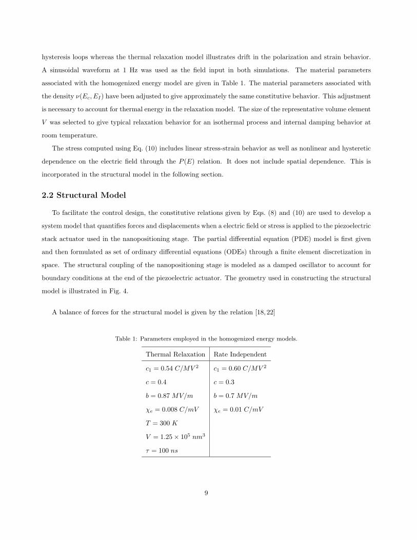
Table 1: Parameters employed in the homogenized energy models.

Thermal Relaxation Rate Independent

c1 = 0.54 C/MV 2 c1 = 0.60 C/MV 2

c = 0.4 c = 0.3

b = 0.87 MV/m b = 0.7 MV/m

χe = 0.008 C/mV χe = 0.01 C/mV

T = 300 K

V = 1.25× 105 nm3

τ = 100 ns

9

0 0.5 1 1.5 20.16

0.18

0.2

0.22

0.24

0.26

Electric field (MV/m)

Pol

ariz

atio

n (C

/m2 )

Neglible RelaxationThermal Relaxation

0 0.5 1 1.5 2−500

0

500

1000

Electric field E (MV/m)

Mic

rost

rain

, ε (

µm/m

)

Negligible RelaxationThermal Relaxation

(a) (b)

Figure 3: Nonlinear and hysteretic homogenized energy model results for minor loop hysteresis typically observed in

ferroelectric materials under zero stress; comparison between the negligible relaxation model and thermal relaxation

model. (a) Electric field versus polarization. (b) Electric field versus longitudinal microstrain.

ρA∂2w

∂t2=

∂Ntot

∂x(11)

where the density of the actuator is denoted by ρ, the cross-section area is A and the displacement is denoted

by w. The total force Ntot acting on the actuator is

������������

������������

L

L

d Lx=0

Fx=L

+wk w

dw/dtc

Mu(t)

Transducer

Figure 4: Piezoelectric stack actuator with damped oscillator used to quantify loads during scanning operations of an

AFM nanopositioning stage. Disturbance forces along the actuator are given by Fd and the control input is u(t).

10

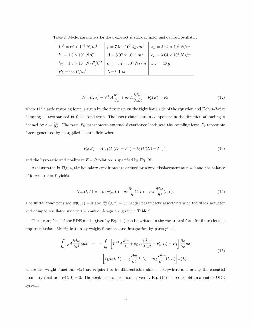
Table 2: Model parameters for the piezoelectric stack actuator and damped oscillator.

Y P = 60× 109 N/m2 ρ = 7.5× 103 kg/m3 kL = 3.04× 106 N/m

h1 = 1.0× 106 N/C A = 5.07× 10−4 m2 cL = 3.04× 102 Ns/m

h2 = 1.0× 103 Nm2/C2 cD = 3.7× 106 Ns/m mL = 40 g

PR = 0.3 C/m2 L = 0.1 m

Ntot(t, x) = Y P A∂w

∂x+ cDA

∂2w

∂x∂t+ Fp(E) + Fd (12)

where the elastic restoring force is given by the first term on the right hand side of the equation and Kelvin-Voigt

damping is incorporated in the second term. The linear elastic strain component in the direction of loading is

defined by ε = ∂w∂x . The term Fd incorporates external disturbance loads and the coupling force Fp represents

forces generated by an applied electric field where

Fp(E) = A[h1(P (E)− P r) + h2(P (E)− P r)2] (13)

and the hysteretic and nonlinear E − P relation is specified by Eq. (8).

As illustrated in Fig. 4, the boundary conditions are defined by a zero displacement at x = 0 and the balance

of forces at x = L yields

Ntot(t, L) = −kLw(t, L)− cL∂w

∂t(t, L)−mL

∂2w

∂t2(t, L). (14)

The initial conditions are w(0, x) = 0 and ∂w∂x (0, x) = 0. Model parameters associated with the stack actuator

and damped oscillator used in the control design are given in Table 2.

The strong form of the PDE model given by Eq. (11) can be written in the variational form for finite element

implementation. Multiplication by weight functions and integration by parts yields

∫ L

0

ρA∂2w

∂t2φdx = −

∫ L

0

[Y MA

∂w

∂x+ cDA

∂2w

∂x∂t+ Fp(E) + Fd

]∂φ

∂xdx

−[kLw(t, L) + cL

∂w

∂t(t, L) + mL

∂2w

∂t2(t, L)

]φ(L)

(15)

where the weight functions φ(x) are required to be differentiable almost everywhere and satisfy the essential

boundary condition w(t, 0) = 0. The weak form of the model given by Eq. (15) is used to obtain a matrix ODE

system.

11

2.2.1 Approximation Method

The piezoelectric stack actuator model given by Eq. (15) is discretized in space followed by a finite-difference

approximation. The transducer is divided into N equal segments over the length [0, L] with points xi = ih, i =

0, 1, . . . , N and step size h = L/N . The spatial basis {φi}Ni=1 is comprised of the linear basis functions

φi(x) =1h

(x− xi−1) , xi−1 ≤ x < xi

(xi+1 − x) , xi ≤ x < xi+1

0 , otherwise

(16)

for i = 1, . . . , N − 1. For i = N , the basis function is defined to be

φN (x) =1h

(x− xN−1) , xN−1 ≤ x < xN

0 , otherwise.(17)

Details describing the basis functions can be found in [18,23].

The approximate solution to Eq. (15) is given by a linear superposition of the basis functions

wN (t, x) =N∑

j=1

wj(t)φj(x) (18)

where wj(t) are the nodal displacement solutions along the length of the transducer.

A second order matrix equation is obtained by substituting wN (t, x) into Eq. (15) with the basis functions

employed as the weight functions. This gives

Mw + CDw + Kw = Fp(E)b + fd (19)

where w(t) = [w1(t), . . . , wN (t)], and M ∈ RN×N , CD ∈ RN×N and K ∈ RN×N denote the mass, damping and

stiffness matrices. The vectors b ∈ RN and fd ∈ RN include the integrated basis functions related to the control

input and disturbance loads, respectively. Components contained within the system matrices and vectors can

be found in [16,18] and in the Appendix.

Formulation of Eq. (19) as a first order system yields

x(t) = Ax(t) + [B(u)](t) + G(t)

x(0) = x0

y(t) = Cx(t)

(20)

12

where x(t) = [~w, ~w]T should not to be confused with the coordinate x. The matrix A incorporates the mass,

damping and stiffness matrices given in Eq. (19) and [B(u)](t) includes the nonlinear input where u(t) is defined

as the electric field. The initial conditions are defined by x0. The output of the system y(t) is a function of the

system states according to the matrix C. In the nanopositioning stage, it is assumed that only the displacement

at x = L is observable which results in C =[

1 0 . . . 0]

with dimension 1 × 2N . External disturbances

are incorporated in G. The system matrix A, input vector B(u) and disturbance load G(t) are

A =

0 I

−M−1K −M−1CD

, B(u) = Fp(u)

0

M−1b

, G(t) =

0

M−1fd(t)

. (21)

The identity matrix, with dimension N ×N , is denoted by I.

A temporal discretization of the system given by Eq. (20) is used to numerically analyze the dynamic

performance. The trapezoid rule is adopted since it is moderately accurate, A-stable, and requires minimal

computer storage capacity. The trapezoidal discretization yields the relation for each iteration

xk+1 = Wxk + V [B(uk)] +12V [G(tk) + G(tk+1)]

x(0) = x0

(22)

where a temporal step size ∆t is employed giving a discretization in time defined by tk = k∆t. The values xk

approximate x(tk). The matrices

W =[I− ∆t

2A

]−1 [I +

∆t

2A

]

V = ∆t

[I− ∆t

2A

]−1(23)

are created once for numerical implementation yielding approximate solutions with O(h2, (∆t)2) accuracy. In

Eq. (22), only values for the control input at the present time tk are included in the temporal discretization to

model dynamics of real-time feedback developed in the following section. This approach is employed since the

control input can only be dependent on the current and previous states.

3. Control Design

We first illustrate the performance and limitations of a PID control design when ferroelectric nonlineari-

ties, hysteresis and relaxation behavior are present in the piezoelectric actuator. The ferroelectric constitutive

behavior is shown to introduce degradation in position accuracy when classical control methods are employed.

13

Improvements in high accuracy tracking is then obtained by implementing a nonlinear optimal control design.

Actuator displacements on the order of tens of microns are chosen for the analysis where it has been demon-

strated that nonlinearities and hysteresis are significant. The reference tracking profile used in the simulations

is based on a typical scan and hold procedure used in nano- and micron-scale materal characterization. This

procedure requires that the specimen translate in the x-direction while holding in the y-direction. At the end of

each scan, the position is held in the x-direction and increased or decreased a small amount in the y-direction

and the procedure is repeated in the negative x-direction. Two scanning frequencies are considered — one

moderate frequency (100 Hz) where relaxation is considered negligible and one low frequency (0.2 Hz) where re-

laxation and creep are significant. The constitutive relations given by Eqs. (6) and (7) are employed to illustrate

operating frequencies where hysteresis and relaxation behavior affect the tracking performance.

3.1 Proportional-Integral-Derivative (PID) Tracking Control

We first consider classical PID control design to demonstrate the need for nonlinear control when operating

in regimes where ferroelectric hysteresis and relaxation is significant. Integral control is first developed by

appending an integral state to Eq. (20) that represents the error dynamics between the piezoelectric actuator

displacement and the prescribed displacement r(t).

The error between the output y(t) and the specified displacement is used to formulate the error dynamics

governed by

xI(t) = Cx(t)− r(t). (24)

The integral state augments the state space system to track the accumulation of error. This gives rise to the

relation

xI(t)

x(t)

=

0 C

0 A

xI(t)

x(t)

+

0

B

u(t)−

1

0

r(t) +

0

G(t)

(25)

and the control input is

u(t) = −[

KI K0

]

xI(t)

x(t)

(26)

where KI is a scalar quantity that represents the integral control gain and K0 is a vector with dimension 1×2N

which includes control gains on the displacements and velocities along the length of the piezoelectric actuator.

14

Therefore K0 includes proportional control KP on the actuator displacement w(t) at x = L and derivative

control KD on the actuator velocity w(t) at x = L (i.e., K0 =[

KP 0 . . . 0 KD 0 . . . 0]).

3.1.1 Numerical Results: PID Control Design

The tracking performance of the nanopositioning stage using PID control is demonstrated using scan rates

conducted at two different frequencies. In the first case, we consider a moderate frequency scan rate at 100

Hz where relaxation behavior is expected to be minimal. The negligible relaxation model based on Eq. (7)

is employed in the constitutive law and the control design for the 100 Hz scanning frequency. In the second

case, a low frequency scan rate of 0.2 Hz is applied to the piezoelectric actuator and the relaxation model

(Eq. (6)) is used to illustrate the additional effect of creep in tracking a reference displacement. In both

cases, the maximum displacement specified to the piezoelectric actuator was 40 µm and the disturbance loads

G(t) were set to zero. Additionally, it was determined that a lumped paramater model (single finite element)

was sufficient to accurately model the piezoelectric actuator dynamics for a 100 Hz scan rate, thus the state

space system reduces to scalar coefficients with N = 1. The lumped parameter model assumes the σ − ε

and E − P are uniform along the rod which has been shown to be a reasonable approximation [20]; however,

in general this approximation is not necessarily valid for all rod structures and operating regimes. In these

cases, implementation of the discretized PDE is necessary. The control gains on the integral state, actuator

displacement and velocity at x = L were adjusted to minimize the error between the prescribed displacement

and the commanded displacement. The values used in the simulations were KI = 1.4× 1012, KP = 1× 108 and

KD = 2000 where the units were N-m and mC- kV. Larger control gains resulted in no improvement in error

reduction and eventually led to an unstable response.

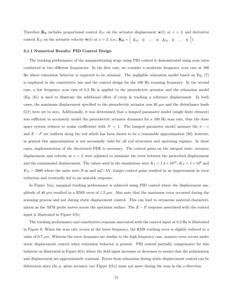
In Figure 5(a), marginal tracking performance is achieved using PID control where the displacement am-

plitude of 40 µm resulted in a RMS error of 1.2 µm. Also note that the maximum error occurred during the

scanning process and not during static displacement control. This can lead to erroneous material characteri-

zation as the AFM probe moves across the specimen surface. The E − P response associated with the control

input is illustrated in Figure 5(b).

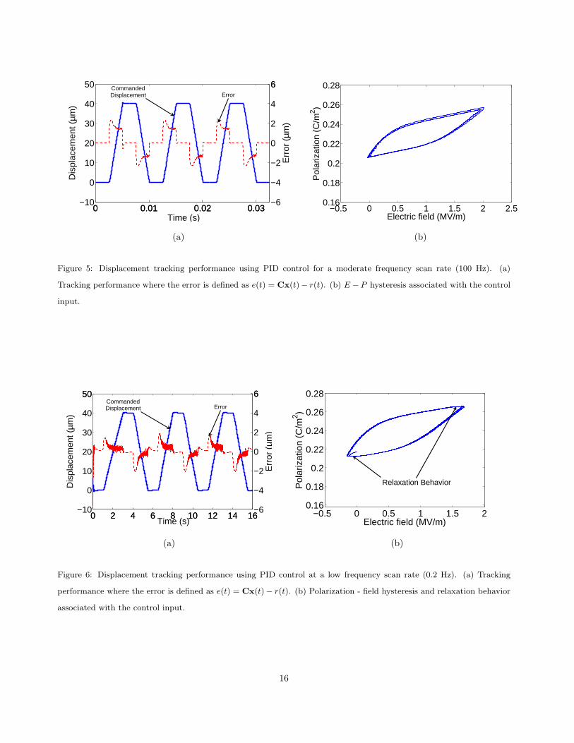
The tracking performance and constitutive response associated with the control input at 0.2 Hz is illustrated

in Figure 6. When the scan rate occurs at the lower frequency, the RMS tracking error is slightly reduced to a

value of 0.7 µm. Whereas the error dynamics are similar to the high frequency case, nonzero error occurs under

static displacement control when relaxation behavior is present. PID control partially compensates for this

behavior as illustrated in Figure 6(b) where the field input increases or decreases to ensure that the polarization

and displacement are approximately constant. Errors from relaxation during static displacement control can be

deleterious since the y−piezo actuator (see Figure 2(b)) must not move during the scan in the x-direction.

15

0 0.01 0.02 0.03−10

0

10

20

30

40

50D

ispl

acem

ent (

µm)

Time (s)0 0.01 0.02 0.03

−6

−4

−2

0

2

4

66

Err

or (

µm)

CommandedDisplacement Error

−0.5 0 0.5 1 1.5 2 2.50.16

0.18

0.2

0.22

0.24

0.26

0.28

Electric field (MV/m)

Pol

ariz

atio

n (C

/m2 )

(a) (b)

Figure 5: Displacement tracking performance using PID control for a moderate frequency scan rate (100 Hz). (a)

Tracking performance where the error is defined as e(t) = Cx(t)− r(t). (b) E −P hysteresis associated with the control

input.

0 2 4 6 8 10 12 14 16−10

0

10

20

30

40

5050

Dis

plac

emen

t (µm

)

Time (s)0 2 4 6 8 10 12 14 16

−6

−4

−2

0

2

4

66

Err

or (

µm)

CommandedDisplacement Error

−0.5 0 0.5 1 1.5 20.16

0.18

0.2

0.22

0.24

0.26

0.28

Electric field (MV/m)

Pol

ariz

atio

n (C

/m2 )

Relaxation Behavior

(a) (b)

Figure 6: Displacement tracking performance using PID control at a low frequency scan rate (0.2 Hz). (a) Tracking

performance where the error is defined as e(t) = Cx(t)− r(t). (b) Polarization - field hysteresis and relaxation behavior

associated with the control input.

16

3.2 Nonlinear Optimal Tracking

Development of the nonlinear optimal tracking control design follows a previous approach focused on negligi-

ble relaxation hysteresis of magnetostrictive actuators for vibration attenuation of beam and plate structures and

tracking control of rod structures [16,24,25]. We summarize here key equations associated with optimal tracking

control and its application in compensating ferroelectric nonlinearities, hysteresis and relaxation behavior.

Optimal tracking control utilizes a cost functional to determine the optimal control input. The cost functional

J =12(Cx(tf )− r(tf ))T P (Cx(tf )− r(tf )) +

∫ tf

t0

[H − λT (t)x(t)

]dt (27)

penalizes the control input and the error between the piezoelectric actuator displacement and the prescibed

displacement where P penalizes large terminal values on the tracking error, H is the Hamiltonian, and λ(t) is

a set of Lagrange multipliers. The Hamiltonian is

H =12

[(Cx(t)− r(t))T Q(Cx(t)− r(t)) + uT (t)Ru(t)

]

+λT [Ax(t) + [B(u)](t) + G(t)]

(28)

where penalties on the tracking error and the control input are given by the variables Q and R, respectively.

The minimum of the cost functional in Eq. (27) is determined under the constraint of the differential equation

given by Eq. (20). By employing Lagrange multipliers an unconstrained minimization problem is constructed

where the stationary condition for the Hamiltonian yields the adjoint relation [26,27]

λ(t) = −ATλ(t)−CTQCx(t) + CTQr(t) (29)

and optimal control input

u(t) = −R−1

(∂B(u)

∂u

)T

λ(t). (30)

The resulting optimality system is

x(t)

λ(t)

=

Ax(t) + [B(u)](t) + G(t)

−ATλ(t)−CTQCx(t) + CTQr(t)

x(t0) = x0

λ(tf ) = CTP (Cx(tf )− r(tf )) .

(31)

17

The force determined from Eq. (13) is included in the input operator [B(u)](t) which directly includes the

nonlinear and hysteretic E − P relation as well as relaxation behavior within the control formulation. This

system of equations results in a two-point boundary value problem which presents challenges in obtaining

a solution for large systems. Furthermore, the nonlinear nature of the input operator precludes an efficient

Riccati formulation.

We first not that Eq. (31) has the general form

z(t) = F(t, z)

E0z(t0) = [x0,0]T

Efz(tf ) = [0,0]T

(32)

where z = [x(t), λ(t)]T and

F(t, z) =

Ax(t) + [B(u)](t) + G(t)

−AT λ(t)−CT QCx(t) + CT Qr(t)

E0 =

I 0

0 0

, Ef =

0 0

−CT PC I

.

(33)

Here I denotes an identity matrix with dimension corresponding to the number of basis functions employed in

the spatial approximation of the state variables. Also note that the prescribed displacement has been restricted

to r(tf ) = 0.

The system given by Eq. (32) is approximated by discretizing the time interval [t0, tf ] with a uniform step

size ∆t at the points t0, t1, · · · , tN = tf . The approximate values of the state solutions and the adjoint at each

time step are denoted by z0, · · · , zN. Whereas several techniques are available to approximate the solution to

Eq. (32), such as finite differences and nonlinear multiple shooting [28], a central difference of the temporal

derivative is utilized here to yield

1∆t

[zj+1 − zj ] =12

[F(tj , zj) + F(tj+1, zj+1)]

E0z0 = [x0,0]T

EfzN = [0,0]

(34)

for j = 0, · · · , N − 1. As summarized in the Appendix, the central difference approximation provides a formu-

lation that can be cast in a analytic LU decomposition to solve the two-point boundary value problem.

18

Equation (34) can be expressed as the problem of finding zh = [z0, · · · , zN ] which solves

F(zh) = 0 . (35)

Equation (35) includes the optimality system at each time step and the boundary conditions. Details are given

in [24].

A quasi-Newton iteration of the form

zk+1h = zk

h + ξkh, (36)

where ξkh solves

F ′(zkh)ξk

h = −F(zkh), (37)

is then used to approximate the solution to the nonlinear system given by Eq. (35). The Jacobian F ′(zkh) has

the form

F ′(zh) =

S0 R0

S1 R1

. . . . . .

SN−1 RN−1

E0 Ef

(38)

where

Si = − 1∆t

I 0

0 I

− 1

2

A ∂

∂λB[u∗i ]

−CT QC −AT

(39)

for Si. The representation for Ri is similar.

Approximate solutions using the quasi-Newton iteration requires inverting the Jabobian to obtain updates to

the states through the iteration procedure. When a large number of time steps and basis functions are required

to represent the structure or device, direct inversion is not feasible. This is avoided by implementing the analytic

LU decomposition. The LU decomposition is identical to the formulation used in previous investigations [24,25]

and is summarized in the Appendix. This gives rise to the following representation of the Jacobian

F ′(zkh) = LU (40)

19

where L and U respectively denote lower and upper triangular matrices. Updates to the state and adjoint

solution at each time step zk+1h are obtained through direct solution of the lower triangular system Lζk

h = −F(zkh)

followed by direct solution of the upper triangular system Uξkh = ζk

h .

3.2.1 Nonlinear Simulation Results

Improvements in tracking control are demonstrated here by implementing the nonlinear optimal control

design. The scanning frequencies used with PID control in Section 3.1.1 illustrate the effectiveness of directly

incorporating ferroelectric constitutive behavior within the nonlinear control design. The values used to penal-

ized the displacement error and control input were Q = 1 × 1016 and R = 1 × 10−8 for both the high and low

frequency scan rates. The penalty on the final state was P = 1.4× 1010.

In Figure 7, the moderate frequency scan rate is simulated using the negligible relaxation polarization kernel

that characterizes typical nonlinearities and hysteresis at this frequency. The RMS error in this case was

0.3 µm for the 40 µm displacement amplitude illustrating a factor of four in error reduction relative to PID

control. Moreover, high performance tracking was achieved with a smaller applied field on the piezoelectric

stack actuator. Here the maximum field input to the stack actuator was less than 1.5 MV/m in comparison to

a maximum field input of 2 MV/m using PID control at 100 Hz (Figure 5b).

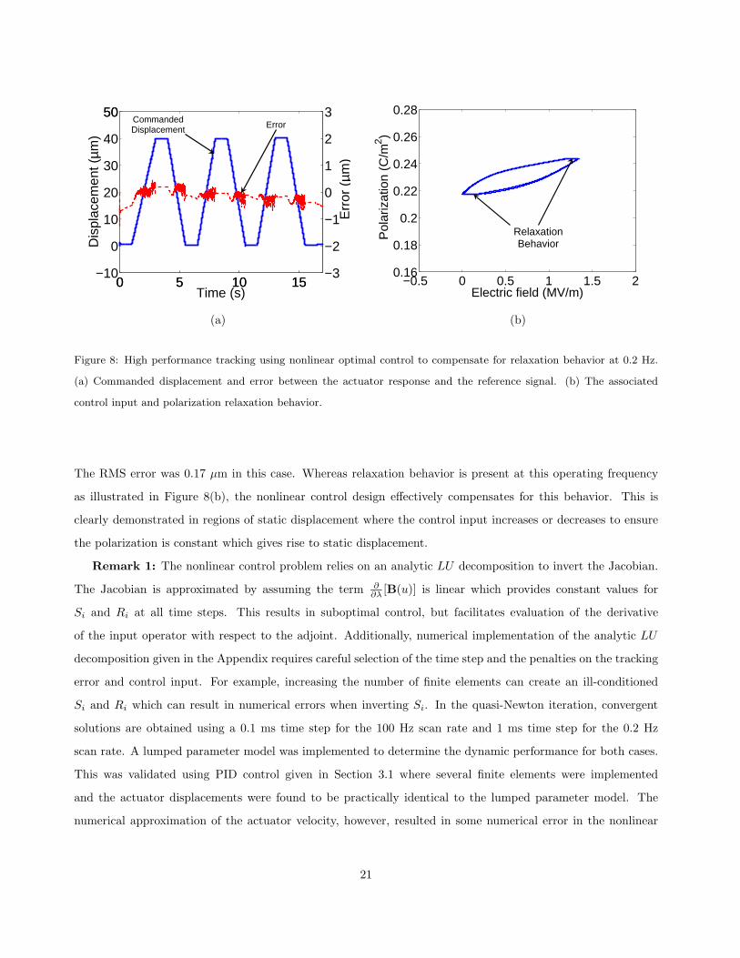
In Figure 8, the nonlinear control design is applied to the piezoelectric actuator using a scan rate of 0.2 Hz.

0 0.01 0.02 0.03−10

0

10

20

30

40

5050

Dis

plac

emen

t (µm

)

Time (s)0 0.01 0.02 0.03

−3

−2

−1

0

1

2

33

Err

or (

µm)

CommandedDisplacement Error

−0.5 0 0.5 1 1.5 20.16

0.18

0.2

0.22

0.24

0.26

0.28

Electric field MV/m

Pol

ariz

atio

n C

/m2

(a) (b)

Figure 7: High performance tracking using open loop nonlinear optimal control with the negligible relaxation constitutive

model at 100 Hz. (a) Commanded displacement and error between the actuator displacement and desired reference signal.

(b) E − P constitutive behavior associated with the control input.

20

0 5 10 15−10

0

10

20

30

40

5050D

ispl

acem

ent (

µm)

Time (s)0 5 10 15

−3

−2

−1

0

1

2

3

Err

or (

µm)

CommandedDisplacement Error

−0.5 0 0.5 1 1.5 20.16

0.18

0.2

0.22

0.24

0.26

0.28

Electric field (MV/m)

Pol

ariz

atio

n (C

/m2 )

RelaxationBehavior

(a) (b)

Figure 8: High performance tracking using nonlinear optimal control to compensate for relaxation behavior at 0.2 Hz.

(a) Commanded displacement and error between the actuator response and the reference signal. (b) The associated

control input and polarization relaxation behavior.

The RMS error was 0.17 µm in this case. Whereas relaxation behavior is present at this operating frequency

as illustrated in Figure 8(b), the nonlinear control design effectively compensates for this behavior. This is

clearly demonstrated in regions of static displacement where the control input increases or decreases to ensure

the polarization is constant which gives rise to static displacement.

Remark 1: The nonlinear control problem relies on an analytic LU decomposition to invert the Jacobian.

The Jacobian is approximated by assuming the term ∂∂λ [B(u)] is linear which provides constant values for

Si and Ri at all time steps. This results in suboptimal control, but facilitates evaluation of the derivative

of the input operator with respect to the adjoint. Additionally, numerical implementation of the analytic LU

decomposition given in the Appendix requires careful selection of the time step and the penalties on the tracking

error and control input. For example, increasing the number of finite elements can create an ill-conditioned

Si and Ri which can result in numerical errors when inverting Si. In the quasi-Newton iteration, convergent

solutions are obtained using a 0.1 ms time step for the 100 Hz scan rate and 1 ms time step for the 0.2 Hz

scan rate. A lumped parameter model was implemented to determine the dynamic performance for both cases.

This was validated using PID control given in Section 3.1 where several finite elements were implemented

and the actuator displacements were found to be practically identical to the lumped parameter model. The

numerical approximation of the actuator velocity, however, resulted in some numerical error in the nonlinear

21

model. To achieve high performance tracking, large jumps in the actuator velocity occur over the scanning

profile particularly at high frequency. This requires a small step size which is not feasible in the quasi-Newton

method due to numerical errors associated with ill-conditioned matrices Si and Ri. This issue is addressed in the

nonlinear problem by penalizing actuator displacement and not the velocity in the cost functional. Additionally,

the control input computed during each iteration is filtered by averaging values over two consectutive time steps

to improve convergence properties. These errors can be potentially reduced further by using adaptive step sizes

near regions of large jumps in the velocity, although more work is required to implement this technique.

Remark 2: The negligible relaxation homogenized energy model has been employed to estimate typical

ferroelectric nonlinearities and hysteresis at the 100 Hz scan rate whereas the relaxation model was implemented

at low frequency to evaluate to effects of charge relaxation and creep. This approach has approximated the

actual rate-dependent hysteresis that may occur over a broad frequency spectrum. The relaxation model is valid

for isothermal processes; however, thermal boundary conditions and heat generation may occur which requires

additional analysis to incorporate these effects into a multi-scale framework over a broad frequency range. In

the present analysis, the negligible relaxation model and relaxation model are assumed to contain comparable

hysteresis effects to illustrate differences tracking performance when relaxation may be present.

3.3 Perturbation Control

In the previous section, a nonlinear open loop control design was shown to provide accurate tracking behavior

by compensating for nonlinear and hysteretic ferroelectric material behavior. However, it is well known that

such open loop controls are not robust with regard to operating uncertainties such as unmodeled constitutive

behavior or disturbance loads. These issues are addressed by implementing perturbation feedback determined

using PI control to improve robustness. The control design presented here can be extended to PID control;

however, additional control gains on the actuator velocity did not improve tracking performance.

The perturbed system consists of first-order variations in the state space system and initial conditions

previously given by Eq. (20),

δx(t) = Aδx(t) + Bδu(t) + δG(t)

δy(t) = Cδx(t) + w(t)

δx(t0) = δx0,

(41)

where δu, δx and δy are first-order variations about the optimal input and system states u∗, x∗ and y∗. The

nonlinear input operator B(u) has been linearized around the optimal input u∗(t). The perturbation in plant

disturbances is denoted by δG(t). In comparison to the output in Eq. (20), measurement noise w(t) has been

22

included in the first-order variation of the output to illustrate robustness in the resulting design. Both the

variation in system noise δG(t) and the measurement noise w(t) are assumed to be random processes with zero

mean. The covariance for the system and measurement noise is defined by E[δG(t)δGT (τ)

]= V δ(t − τ) and

E[w(t)wT (τ)

]= Wδ(t− τ) with the joint property E

[δG(t)wT (τ)

]= 0.

Proportional Integral (PI) control is implemented in the perturbed system in a manner analogous to the

approach summarized in Section 3.1. An integrator state associated with error in the perturbed states is

introduced

δxI(t) = Cδx(t) + e(t). (42)

where e(t) = Cx(t)− r(t). This results in an augmented perturbation system given by

δxI(t)

δx(t)

=

0 C

0 A

δxI(t)

δx(t)

+

0

B

δu(t) +

1

0

e(t) +

0

δG(t)

(43)

The control input is

δu(t) = −[

KδI Kδ

0

]

δxI(t)

δx(t)

(44)

where the integral control gain KδI is a scalar coefficient and the proportional Kδ

P and derivative KδD control

gains are included in the vector Kδ0 similar to the control gain presented in Section 3.1. As previously mentioned,

derivative control can be included, although only PI perturbation control is considered here.

The nanopositioning stage relies on position feedback using a laser and a photodiode. A certain level of

sensor noise is expected to be present which can degrade tracking performance from sensor feedback. A Kalman

filter is used to accommodate measurement noise in the feedback sensor, as well as unmeasured states, by

introducing the state estimator

δ ˙x(t) = Aδx(t) + Bδu(t) + L(t) [δy(t)−Cδx(t)]

δx(t0) = δx0

(45)

into the perturbation system. Here δx0 is the estimated initial conditions and L(t) is the Kalman gain. A

similar approach can be found in [16].

Key equations used in determining the Kalman gain are summarized here; see [29,30] for additional details.

The Kalman gain is determined from the error covariance Υ(t) = E[eL(t)eT

L(τ)]

where the error is associated

with first order variations in the error dyanmics

23

eL(t) = δx(t)− δ ˙x(t). (46)

By substituting Eqs. (41) and (45) into Eq. (46), the error is determined by the convolution integral

eL(t) = Φ(t, t0)eL(t0) +∫ t

t0

Φ(t, τ) [δG(τ)− L(τ)w(τ)] dτ (47)

where Φ(t, t0) is the state transition matrix. A differential Riccati equation is obtained by manipulating the

equation for error covariance; see [29, 30] for details. Whereas this yields a time-dependent Kalman gain, a

steady state solution is often sufficient to accurately estimate the system states. The steady-state Kalman gain

is employed here which is determined from the algebraic Riccati equation

AΥ(t) + Υ(t)AT −Υ(t)CT W−1CΥ(t) + V = 0 (48)

with the initial conditions Υ(t0) = Υ0. The steady-state Kalman gain is then given by

L = ΥCT W−1. (49)

In summary, the matrix system

δxI(t)

δx(t)

δ ˙x(t)

=

0 0 C

−BKI A −BK0

−BKI LC A−BK0 − LC

δxI(t)

δx(t)

δx(t)

+

e(t)

δG(t)

Lδw(t)

δxI(t0) = 0

δx(t0) = δx0

δx(t0) = δx0.

(50)

governing the dynamics of the perturbed state space system with PI control and Kalman filter is solved to

obtain the system response when perturbation feedback of the estimated states is implemented.

3.3.1 Numerical Results

The hybrid nonlinear control method using PI perturbation feedback is implemented numerically using a

temporal discretization method similar to Eq. (22). Since the error e(t) is only known at the present and past

time steps, the temporal discretization of Eq. (50) is formulated as

24

δX k+1 = WδXk + VEk + 12V [Nk + Nk+1]

X (0) = X0

(51)

where δXk =[

δxIk δxk δxk

]T

, Ek =[

ek 0 0]T

and Nk =[

0 δGk wk

]T

for each time step

tk. The matrices W and V are similar to those used in Eq. (22) except the A matrix contains the input

vector, control gains, and Kalman gains given in the form of the matrix in Eq. (50). This form of the temporal

discretization gives a direct comparison of performance improvements relative to the PID control given in

Section 3.1. The control gains were KδI = 5 × 1017 and Kδ

P = 1 × 1011 using the units N-m and mC-kV. The

values used in determining the Kalman gains were V = 5× 106 and W = 5× 10−6 while the measurement noise

was a random signal with amplitude 1 µm. The first order variation in disturbance noise was set to zero.

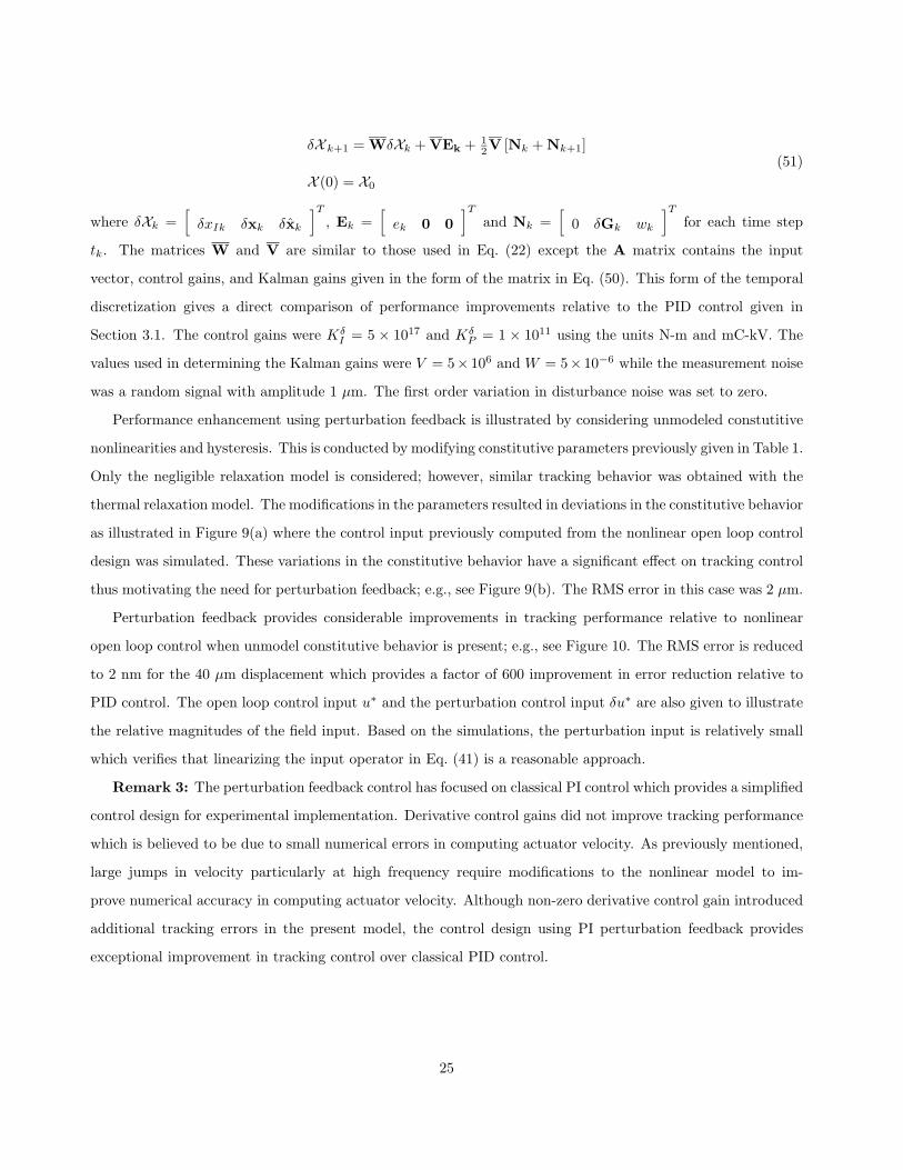
Performance enhancement using perturbation feedback is illustrated by considering unmodeled constutitive

nonlinearities and hysteresis. This is conducted by modifying constitutive parameters previously given in Table 1.

Only the negligible relaxation model is considered; however, similar tracking behavior was obtained with the

thermal relaxation model. The modifications in the parameters resulted in deviations in the constitutive behavior

as illustrated in Figure 9(a) where the control input previously computed from the nonlinear open loop control

design was simulated. These variations in the constitutive behavior have a significant effect on tracking control

thus motivating the need for perturbation feedback; e.g., see Figure 9(b). The RMS error in this case was 2 µm.

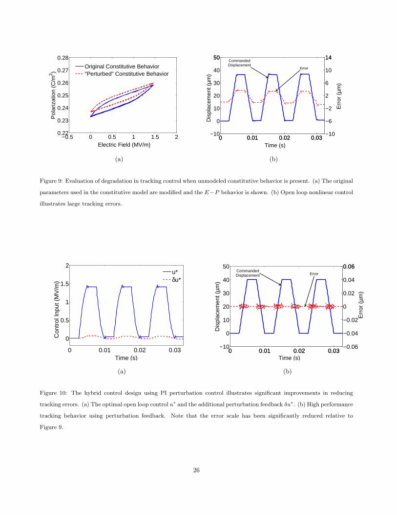
Perturbation feedback provides considerable improvements in tracking performance relative to nonlinear

open loop control when unmodel constitutive behavior is present; e.g., see Figure 10. The RMS error is reduced

to 2 nm for the 40 µm displacement which provides a factor of 600 improvement in error reduction relative to

PID control. The open loop control input u∗ and the perturbation control input δu∗ are also given to illustrate

the relative magnitudes of the field input. Based on the simulations, the perturbation input is relatively small

which verifies that linearizing the input operator in Eq. (41) is a reasonable approach.

Remark 3: The perturbation feedback control has focused on classical PI control which provides a simplified

control design for experimental implementation. Derivative control gains did not improve tracking performance

which is believed to be due to small numerical errors in computing actuator velocity. As previously mentioned,

large jumps in velocity particularly at high frequency require modifications to the nonlinear model to im-

prove numerical accuracy in computing actuator velocity. Although non-zero derivative control gain introduced

additional tracking errors in the present model, the control design using PI perturbation feedback provides

exceptional improvement in tracking control over classical PID control.

25

−0.5 0 0.5 1 1.5 20.22

0.23

0.24

0.25

0.26

0.27

0.28

Electric Field (MV/m)

Pol

ariz

atio

n (C

/m2 )

Original Constitutive Behavior"Perturbed" Constitutive Behavior

0 0.01 0.02 0.03−10

0

10

20

30

40

5050

Dis

plac

emen

t (µm

)

0 0.01 0.02 0.03−10

−6

−2

2

6

10

1414

Err

or (

µm)

CommandedDisplacement

Error

Time (s)

(a) (b)

Figure 9: Evaluation of degradation in tracking control when unmodeled constitutive behavior is present. (a) The original

parameters used in the constitutive model are modified and the E−P behavior is shown. (b) Open loop nonlinear control

illustrates large tracking errors.

0 0.01 0.02 0.03

0

0.5

1

1.5

2

Time (s)

Con

trol

Inpu

t (M

V/m

)

u*δu*

0 0.01 0.02 0.03−10

0

10

20

30

40

50

Dis

plac

emen

t (µm

)

Time (s)0 0.01 0.02 0.03

−0.06

−0.04

−0.02

0

0.02

0.04

0.060.06

Err

or (

µm)

CommandedDisplacement Error

(a) (b)

Figure 10: The hybrid control design using PI perturbation control illustrates significant improvements in reducing

tracking errors. (a) The optimal open loop control u∗ and the additional perturbation feedback δu∗. (b) High performance

tracking behavior using perturbation feedback. Note that the error scale has been significantly reduced relative to

Figure 9.

26

4. Concluding Remarks

A hybrid nonlinear optimal control design has been applied to a nanopositioning stage for both quasi-static

and high frequency (100 Hz) scanning rates for applications where nanoscale resolution is critical. Ferroelectric

material behavior was incorporated into the control design using a homogenized energy model that accounts for

local residual interaction fields and variations in the coercive field. Material parameters were chosen to represent

typical hysteresis behavior for operating frequencies that range from tens to hundreds of Hertz. Relaxation

behavior was incorporated into the constitutive model to account for creep during quasi-static actuation. The

hybrid control design significantly improved reduction in tracking errors relative to PID control where the error

was reduced by over two orders of magnitude for the high frequency scan rate. Furthermore, the improvement

in tracking performance was achieved using a smaller field input which may have implications in applications

were energy efficiency is critical.

Acknowledgments

The authors gratefully acknowledge support from the Air Force Office of Scientific Research through grant

AFOSR-FA9550-04-1-0203.

Appendix

A. Mathematical Relations

Matrix and Vector Relations

The matrices and vectors given in Section 2.2 are formulated using linear basis functions. The approximate

displacements in Eq. (18) are substituted into the variational form of the dynamic equation Eq. (15) which gives

N∑j=1

wj(t)∫ L

0

ρAφiφjdx +N∑

j=1

wj(t)∫ L

0

cDAφ′iφ′jdx +

N∑j=1

wj(t)∫ L

0

Y MAφ′iφ′jdx = Fmag(H)

∫ L

0

φ′idx

+∫ L

0

Fdφidx− (kLwN (t)φN (L) + cLwN (t)φN (L) + mLwNφN (L)) φN (L) .

The global mass, stiffness, and damping matrices have the components

[M]ij =

∫ L

0

ρAφiφjdx , i 6= N or j 6= N

∫ L

0

ρAφiφjdx + mL , i = N or j = N

27

[CD]ij =

∫ L

0

cDAφ′iφ′jdx , i 6= N or j 6= N

∫ L

0

cDAφ′iφ′jdx + cL , i = N or j = N

[K]ij =

∫ L

0

Y MAφ′iφ′jdx , i 6= N or j 6= N

∫ L

0

Y MAφ′iφ′jdx + kL , i = N or j = N

whereas the force vectors have the components

[fd]i =∫ L

0

Fdφidx , [b]i =∫ L

0

φ′idx.

Details regarding the formulation of these matrices can be found in Chapter 8 of [18].

LU Decomposition

The Jacobian given by Eq. (38) is written in terms of a LU decomposition to avoid matrix inversion when

considering large systems. The analytic form of the decomposition used in the simulations is

L =

S0

S1

. . .

SN−1 0

E0 −E0(S−10 R0) · · · E0

N−2∏i=0

(−1)i(S−1i Ri) Ef + E0

N−1∏i=0

(−1)i(S−1i Ri)

U =

I S−10 R0

I S−11 R1

. . . . . .

I S−1N−1RN−1

I

.

28

This form of the matrix system reduces the computation to solving 2N × 2N systems for each time step

separately.

References

[1] Park, S.-E., and Shout, T., 1997. “Ultrahigh strain and piezoelectric behavior in relaxor based ferroelectric

single crystals”. J. Appl. Phys., 82(4), pp. 1804–18011.

[2] Liu, T., and Lynch, C., 2003. “Ferroelectric properties of [110], [001], and [111] poled relaxor single crystals:

measurements and modeling”. Acta. Mater., 51, pp. 407–416.

[3] McLaughlin, B., Liu, T., and Lynch, C., 2004. “Relaxor ferroelectric PMN-32%PT crystals under stress

and electric field loading: I-32 mode measurements”. Acta. Mater., 52, pp. 3849–3857.

[4] Main, J., Garcia, E., and Newton, D., 1995. “Precision position control of piezoelectric actuators using

charge feedback”. J. Guid. Control Dynam., 18(5), pp. 1068–1073.

[5] Main, J., Garcia, E., Newton, D., Massengil, L., and Garcia, E., 1996. “Efficient power amplifiers for

piezoelectric applications”. Smart Mater Struct, 5(6), pp. 766–775.

[6] Wong, C., Jeon, Y., Barbastathis, G., and Kim, S.-K., 2004. “Analog piezoelectric-driven tunable gratings

with nanometer resolution”. J. Microelectromech. S., 13(6), pp. 998–1005.

[7] Gruverman, A., Cao, W., Bhaskar, S., and Dey, S., 2004. “Investigation of Pb(Zr,Ti)O3/GaN heterostruc-

tures by scanning probe microscopy”. Appl. Phys. Lett., 84(25), pp. 5153–5155.

[8] Sugimoto, Y., Abe, M., Hirayama, S., Oyabu, N., Custance, O., and Morita, S., 2005. “Atom inlays

performed at room temperature using atomic force microscopy”. Nat. Mater., 4, pp. 156–159.

[9] Tang, Q., Zhang, Y., Chen, L., Yan, F., and Wong, R., 2005. “Protein delivery with nanoscale precision”.

Nanotechnology, 16, pp. 1062–1068.

[10] Schitter, G., Menold, P., Knapp, H., Allgower, F., and Stemmer, A., 2003. “High performance feedback

for fast scanning atomic force microscopes”. Rev. Sci. Instrum., 72(8), pp. 3320–3327.

[11] Sebastion, A., and Salapaka, S., 2003. “H∞ loop shaping design for nano-positioning”. IEEE Proc. Amer.

Control Conf., pp. 3708–3713.

[12] Salapaka, S., Sebastian, A., Cleveland, J., and Salapaka, M., 2002. “High bandwidth nano-positioner: A

robust control approach”. Rev. Sci. Instrum., 73(9), pp. 3232–3241.

29

[13] Croft, D., and Devasia, S., 1999. “Vibration compensation for high speed scanning tunneling microscopy”.

Rev. Sci. Instrum., 70(12), pp. 4600–4605.

[14] Zou, Q., and Devasia, S., 2004. “Preview-based optimal inversion for output tracking: Applications to

scanning tunneling microscopy”. IEEE T. Contr. Syst. T., 12(3), pp. 375–386.

[15] Smith, R., Salapaka, M., Hatch, A., Smith, J., and De, T., 2002. “Model development and inverse com-

pensator design for high speed nanopositioning”. Proc. 41nd IEEE Conf. Decision Control, pp. 3652–3657.

[16] Oates, W., and Smith, R. “Optimal tracking using magnetostricive actuators operating in the nonlinear

and hysteretic regime”. submitted to J. Dyn. Syst.-T. ASME.

[17] Smith, R., Hatch, A., De, T., Salapaka, M., del Rosario, R., and Raye, J. “Model development for atomic

force microscope mechanisms”. CRSC-TRO5-25, SIAM J. Appl. Math, submitted.

[18] Smith, R., 2005. Smart Material Systems: Model Development. SIAM, Philadelphia, PA.

[19] Smith, R., Seelecke, S., Ounaies, Z., and Smith, J., 2003. “A free energy model for hysteresis in ferroelectric

materials”. J. Intell. Mater. Syst. Struct., 14(11), pp. 719–739.

[20] Smith, R., Hatch, A., Mukherjee, B., and Liu, S., 2005. “A homogenized energy model for hysteresis in

ferroelectric materials: General density formulations”. J. Intell. Mater. Syst. Struct., 16(9), pp. 713–732.

[21] Smith, R., Seelecke, S., Dapino, M., and Ounaies, Z., 2005. “A unified framework for modeling hysteresis

in ferroic materials”. J. Mech. Phys. Solids, 54(1), pp. 46–55.

[22] Dapino, M., Smith, R., and Flatau, A., 2000. “A structural strain model for magnetostrictive transducers”.

IEEE T. Magn., 36(3), pp. 545–556.

[23] Reddy, J., 1993. An Introduction to the Finite Element Method. McGraw-Hill, New York, NY.

[24] Smith, R., 1995. “A nonlinear optimal control method for magnetostrictive actuators”. J. Intell. Mater.

Syst. Struct., 9(6), pp. 468–486.

[25] Oates, W., and Smith, R. “Nonlinear optimal control techniques for vibration attenuation using nonlinear

magnetostricive actuators”. submitted to J. Intell. Mater. Sys. Struct.

[26] Bryson, A., and Ho, Y.-C., 1969. Applied Optimal Control. Blasidell Publishing Company, Waltham, MA.

[27] Lewis, F., and Syrmos, V., 1995. Optimal Control. John Wiley and Sons, New York, NY.

30

[28] Ascher, U., Mattheij, R., and Russell, R., 1995. Numerical Solution of Boundary Value Problems for

Ordinary Differential Equations. SIAM Classics in Applied Mathematics.

[29] Lewis, F., 1986. Optimal Estimation With an Introduction to Stochastic Control Theory. John Wiley and

Sons, New York, NY.

[30] Bay, J., 1999. Fundamentals of Linear State Space Systems. WCB McGraw-Hill.

31