nonlinear control lecture 4: stability analysis iele.aut.ac.ir/~abdollahi/lec_3_n10.pdf · outline...
TRANSCRIPT

Outline Autonomous Systems Invariance Principle Linear System and Linearization Lyapunov and Lasalle Appl.
Nonlinear ControlLecture 4: Stability Analysis I
Farzaneh Abdollahi
Department of Electrical Engineering
Amirkabir University of Technology
Fall 2010
Farzaneh Abdollahi Nonlinear Control Lecture 4 1/70

Outline Autonomous Systems Invariance Principle Linear System and Linearization Lyapunov and Lasalle Appl.
Autonomous SystemsLyapunov StabilityVariable Gradient MethodRegion of Attraction
Invariance Principle
Linear System and Linearization
Lyapunov and Lasalle Theorem ApplicationExample: Robot ManipulatorControl Design Based on Lyapunov’s Direct MethodEstimating Region of Attraction
Farzaneh Abdollahi Nonlinear Control Lecture 4 2/70

Outline Autonomous Systems Invariance Principle Linear System and Linearization Lyapunov and Lasalle Appl.
StabilityI Stability theory is divided into three parts:
1. Stability of equilibrium points2. Stability of periodic orbits3. Input/output stability
I An equilibrium point (Equ. pt.) is:I Stable if all solutions starting at nearby points stay nearby.I Asymptotically Stable if all solutions starting at nearby points not only stay
nearby, but also tend to the Equ. pt. as time approaches infinity.I Exponentially Stable, if the rate of converging to the Equ. pt. is
exponentially.I Lyapunov stability theorems give sufficient conditions for stability,
asymptotic stability, and so on.
I Lyapunov stability analysis can be used to show boundedness of thesolution even when the system has no equilibrium points.
I The theorems provide necessary conditions for stability are so-calledconverse theorems.
Farzaneh Abdollahi Nonlinear Control Lecture 4 3/70
Outline Autonomous Systems Invariance Principle Linear System and Linearization Lyapunov and Lasalle Appl.
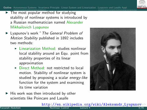
I The most popular method for studyingstability of nonlinear systems is introduced bya Russian mathematician named AlexanderMikhailovich Lyapunov
I Lyapunov’s work ”The General Problem ofMotion Stability published in 1892 includestwo methods:
I Linearization Method: studies nonlinearlocal stability around an Equ. point fromstability properties of its linearapproximation
I Direct Method: not restricted to localmotion. Stability of nonlinear system isstudied by proposing a scalar energy-likefunction for the system and examiningits time variation
I His work was then introduced by otherscientists like Poincare and Lasalle
http://en.wikipedia.org/wiki/Aleksandr_LyapunovFarzaneh Abdollahi Nonlinear Control Lecture 4 4/70
Outline Autonomous Systems Invariance Principle Linear System and Linearization Lyapunov and Lasalle Appl.
Autonomous Systems
I Consider the autonomous system:x = f (x)
where f : D −→ Rn is a locally Lip. function on a domain D ⊂ Rn.
I Let x ∈ D be an Equ. point, that is f (x) = 0.
I Objective: To characterize stability of x .I without loss of generality (wlog), let x = 0
I If x 6= 0, introduce a coordinate transformation: y = x − x , thenI y = x = f (y + x) = g(y) with g(0) = 0
Farzaneh Abdollahi Nonlinear Control Lecture 4 5/70

Outline Autonomous Systems Invariance Principle Linear System and Linearization Lyapunov and Lasalle Appl.
I The Equ. point x = 0 of x = f (x) is:I stable, if for each ε > 0, ∃ δ = δ(ε) > 0
s.t.
‖x(0)‖ < δ =⇒ ‖x(t)‖ < ε ∀t ≥ 0
I unstable, if it is not stableI asymptotically stable, if it is stable andδ can be chosen s.t.
‖x(0)‖ < δ =⇒ limt−→∞
x(t) = 0
I ∴ Lyapunov stability means that thesystem trajectory can be kept arbitraryclose to the origin by starting sufficientlyclose to it.
I An Equ. point which is Lypunov stabilebut not asymptotically stable is calledMarginally stable
Farzaneh Abdollahi Nonlinear Control Lecture 4 6/70

Outline Autonomous Systems Invariance Principle Linear System and Linearization Lyapunov and Lasalle Appl.
I Example: Van Der Pol OscillatorI Van der pol oscillator dynamics:
x1 = x2
x2 = −x1 + (1− x1)2x2
I All system trajectories start except fromorigin, asymptotically approaches a limitcycle.
I ∴ Even the system states remain aroundthe Equ. point in a certain sense, theycan not stay arbitrarily close to it.
I So the Equ. point is unstable.
I Implicit in Lyapunov stability condition isthat the sol. are defined ∀t ≥ 0.
I This is not guaranteed by local Lip.I The additional condition imposed by
Lyapunov theorem will ensure global existenceof sol.
Farzaneh Abdollahi Nonlinear Control Lecture 4 7/70

Outline Autonomous Systems Invariance Principle Linear System and Linearization Lyapunov and Lasalle Appl.
Lyapunov StabilityI Physical Motivation
I Consider the pendulum example (recall Lecture 2):
x1 = x2
x2 =−g
lsinx1 −
k
mx2
I In first period it has two Equ. pts. (x1 = 0, x2 = 0) & (x1 = π, x2 = 0)
I For frictionless pendulum, i.e. k = 0 : trajectories are closed orbits inneighborhood of 1st Equ. pt. ε− δ requirement for stability is satisfied.
I However, it is not asymptotically stable.
I For Pendulum with friction, i.e. k > 0the 1st Equ. pt. is a stable focus ε− δ requirement for asymptoticstability is satisfied.the 2nd Equ. pt. is a saddle point ε− δ requirement is not satisfied it is unstable
Farzaneh Abdollahi Nonlinear Control Lecture 4 8/70

Outline Autonomous Systems Invariance Principle Linear System and Linearization Lyapunov and Lasalle Appl.
I To generalize the phase-plane analysis, consider the energy associatedwith the pendulum:
E (x) =1
2x22 +
∫ x1
0
g
lsin y dy =
1
2x22 +
g
l(1− cosx1), E (0) = 0
I If k = 0, system is conservative, i.e. there is no dissipation of energy:I E = constant during the motion of the system.I ∴ dE
dt = 0 along the traj. of the system.
I If k > 0, energy is being dissipatedI dE
dt < 0 along the traj. of the system.I ∴ E starts to decrease until it eventually reaches zero, at that pt. x = 0.
I Lyapunov showed that certain other function can be used instead ofenergy function to determine stability of an Equ. pt.
Farzaneh Abdollahi Nonlinear Control Lecture 4 9/70
Outline Autonomous Systems Invariance Principle Linear System and Linearization Lyapunov and Lasalle Appl.
Lyapunov’s Direct Method:
I Let x = 0 be an Equ. pt. for x = f (x). Let V : D −→ R, D ⊂ Rn be acontinuously differentiable function on a neighborhood D of x = 0, s.t.
1. V (0) = 02. V (x) > 0 in D − 03. V (x)≤0 in D
Then x = 0 is stable.Moreover, if V (x)<0 in D − 0 then x = 0 is asymptotically stable.
I The continuously differentiable function V (x) is called a Lyapunovfunction.
I The surface V (x) = c , for some c > 0 is called a Lyapunov surface orlevel surface.
Farzaneh Abdollahi Nonlinear Control Lecture 4 10/70

Outline Autonomous Systems Invariance Principle Linear System and Linearization Lyapunov and Lasalle Appl.
Lyapunov Stability
I when V ≤ 0 when a trajectory crosses a Lyapunov surface V (x) = c , it moves insidethe set Ωc = x ∈ Rn|V (x) ≤ c and traps inside Ωc .
I when V < 0 trajectories move from one level surface to an inner level with smaller ctill V (x) = c shrinks to zero as time goes on
Farzaneh Abdollahi Nonlinear Control Lecture 4 11/70

Outline Autonomous Systems Invariance Principle Linear System and Linearization Lyapunov and Lasalle Appl.
Lyapunov StabilityI A function satisfying V (0) = 0 & V (x) > 0 in D − 0 is said to be
Positive Definite (p.d.)
I If it satisfies a weaker condition V (x) ≥ 0 for x 6= 0 is said to be PositiveSemi-Definite (p.s.d.)
I A function is Negative Definite (n.d.) or Negative Semi-Definite (n.s.d.)if −V (x) is p.d. or p.s.d., respectively.
I Lyapunov theorem states that:The origin is stable if there is a continuously differentiable, p.d. functionV (x) s.t. V (x) is n.s.d., and is asymptotically if V (x) is n.d.
I Note that when x is a vector:
V (x) =∂V
∂xf (x) =
n∑i=1
∂V
∂xixi =
n∑i=1
∂V
∂xifi =
[∂V∂x1
· · · ∂V∂xn
] f1...
fn
Farzaneh Abdollahi Nonlinear Control Lecture 4 12/70

Outline Autonomous Systems Invariance Principle Linear System and Linearization Lyapunov and Lasalle Appl.
Lyapunov Stability
I A class of scalar functions for which sign definition can be easily checkedis ”quadratic functions:”
V (x) = xT Px =n∑
i=1
n∑j=1
xixjPij
where P = PT is a real matrix.
I V (x) is p.d./p.s.d. iff λiP > 0 or λiP ≥ 0, i = 1...n
I λiP > 0 or λiP ≥ 0, i = 1...n iff all leading principle minors of Pare positive or non-negative, respectively.
I If V (x) is p.d. (p.s.d.), we say the matrix P is p.d. (p.s.d.) and writeP > 0 (P ≥ 0).
Farzaneh Abdollahi Nonlinear Control Lecture 4 13/70

Outline Autonomous Systems Invariance Principle Linear System and Linearization Lyapunov and Lasalle Appl.
Example 1
V (x) = ax21 + 2x1x3 + ax2
2 + 4x2x3 + ax23
=[
x1 x2 x3
] a 0 10 a 21 2 a
x1
x2
x3
= xT Px
I The leading principle minors are
det(a) = a; det
[a 00 a
]= a2; det
a 0 10 a 21 2 a
= a(a2 − 5)
∴V (x) is p.s.d. if a ≥√
5, V (x) is p.d. if a >√
5I For n.d. the leading principle minors of
I −P should be positive. ORI P should alternate in sign with the first one neg. (odds: neg., even: pos.)
∴V (x) is n.s.d. if a ≤ −√
5, V (x) is n.d. if a < −√
5,V (x) is sign indefinite for −
√5 < a <
√5
Farzaneh Abdollahi Nonlinear Control Lecture 4 14/70

Outline Autonomous Systems Invariance Principle Linear System and Linearization Lyapunov and Lasalle Appl.
Example 2
I Consider x = −g(x) where g(x) is locally Lip. on(−a, a) & g(0) = 0, xg(x) > 0, ∀x 6= 0, x ∈ (−a, a). stability?
I origin is Equ. pt.I Solution 1:
I starting on either side of the origin will have to move toward the origin dueto the sign of x
I ∴ Origin is an isolated Equ. pt. and is asymptotically stable.
I Solution 2: using Lypunov theorem:I Consider the function V (x) =
∫ x
0g(y)dy over D = (−a, a).
I V (x) is continuously differentiable, V (0) = 0 and V (x) > 0, ∀x 6= 0 . Vis a valid Lyapunov candidate
I To see if it is really a Lyap. fcn, we have to take its derivative along systemtrajectory: V (x) = ∂V
∂x (−g(x)) = −g2(x) < 0, ∀x ∈ D − 0I ∴ V (x) is a valid Lyap. fcn the origin is asymptotically stable.
Farzaneh Abdollahi Nonlinear Control Lecture 4 15/70

Outline Autonomous Systems Invariance Principle Linear System and Linearization Lyapunov and Lasalle Appl.
Example 3: Frictionless Pendulum
x1 = x2
x2 =−g
lsinx1
I Study stability of the Equ. pt. at the origin.
I A natural Lyap. fcn is the energy fcn:
V (x) =g
l(1− cosx1) +
1
2x22
I V (0) = 0 and V (x) is p.d. over the domain −2π ≤ x1 ≤ 2π.
I ∴V = gl x1sinx1 + x2x2 = g
l x2sinx1 − gl x2sinx1 = 0
I V (x) satisfies the condition of the Lyap. Theorem origin is stable
Farzaneh Abdollahi Nonlinear Control Lecture 4 16/70

Outline Autonomous Systems Invariance Principle Linear System and Linearization Lyapunov and Lasalle Appl.
Example 4: Pendulum with Frictionx1 = x2
x2 =−g
lsinx1 −
k
mx2
I Take the energy fcn as a Lyap. fcn candidate
V (x) =g
l(1− cosx1) +
1
2x22
I V = − kmx2
2
I V (x) is n.s.d. It is not since n.d. since V = 0 for x2 = 0 and all x1 6= 0.the origin is only stable.
I But, phase portrait showed asymptotic stability!!
I Toward this end, let’s choose:
V (x) =1
2xT Px +
g
l(1− cosx1)
Farzaneh Abdollahi Nonlinear Control Lecture 4 17/70
Outline Autonomous Systems Invariance Principle Linear System and Linearization Lyapunov and Lasalle Appl.
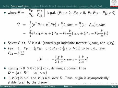
I where P =
[P11 P12
P12 P22
]is p.d. (P11 > 0, P22 > 0, P11P22 − P2
12 > 0)
V =1
2(xT Px + xT Px) +
g
lx1sinx1 =
g
l(1− P22)x2sinx1
− g
lP12x1sinx1 + (P11 − P12
k
m)x1x2 + (P12 − P22
k
m)x2
2
I Select P s.t. V is n.d. (cancel sign indefinite factors: x2sinx1 and x1x2)
I P22 = 1, P11 = kmP12, 0 < P12 <
km (for V (x) to be p.d., take
P12 = 12
km )
∴V = −1
2
g
l
k
mx1sinx1 −
1
2
k
mx22
I x1sinx1 > 0 ∀ 0 < |x1| < π, defining a domain D byD = x ∈ R2| |x1| < π
I ∴ V (x) is p.d. and V is n.d. over D. Thus, origin is asymptoticallystable (a.s.) by the theorem.
Farzaneh Abdollahi Nonlinear Control Lecture 4 18/70

Outline Autonomous Systems Invariance Principle Linear System and Linearization Lyapunov and Lasalle Appl.
How Search for A Lyapunov Function?I Lyapunov theorem is only sufficient.
I Failure of a Lyap. fcn candidate to satisfy the theorem does not meanthe Equ. pt. is unstable.
I Variable Gradient MethodI Idea is working backward:
I Investigated an expression for V (x) and go back to choose the parametersof V (x) so as to make V (x) n.d. (n.s.d)
I Let V = V (x) and g(x) = ∇xV =(
∂V∂x
)TI Then V = ∂V
∂x f = gT fI Choose g(x) s.t. it would be the gradient of a p.d. fcn V and make V n.d.
(n.s.d)I g(x) is the gradient of a scalar fcn iff the Jacobian matrix ∂g
∂x is symmetric:
∂gi
∂xj=∂gj
∂xi, ∀i , j = 1, ..., n
Farzaneh Abdollahi Nonlinear Control Lecture 4 19/70

Outline Autonomous Systems Invariance Principle Linear System and Linearization Lyapunov and Lasalle Appl.
Variable Gradient MethodI Select g(x) s.t. gT (x)f (x) is n.d.
I Then, V (x) is computed from the integral:
V (x) =
∫ x
0g(y)dy =
∫ x
0
n∑i=1
gi (y)dyi
I The integration is taken over any path joining the origin to x . This canbe done along the axes:
V (x) =
∫ x1
0g1(y1, 0, ..., 0)dy1 +
∫ x2
0g2(x1, y2, 0, ..., 0)dy2
+ ...+
∫ xn
0gn(x1, x2, ..., yn)dyn
I By leaving some parameters of g undetermined, one would try to choosethem so that V is p.d.
Farzaneh Abdollahi Nonlinear Control Lecture 4 20/70

Outline Autonomous Systems Invariance Principle Linear System and Linearization Lyapunov and Lasalle Appl.
Example 5:
x1 = x2
x2 = −h(x1)− ax2
where a > 0, h(.) is locally Lip.,h(0) = 0, yh(y) > 0, ∀ y 6= 0, y ∈ (−b, c), b, c > 0.
I The pendulum is a special case of this system.
I Find proper Lypunov function?
I Applying variable gradient method, we must find g(x) s.t. ∂g1∂x2
= ∂g2∂x1
I V (x) = g1(x)x2 − g2(x)(h(x1) + ax2) < 0, ∀x 6= 0 and
V (x) =
∫ x
0gT (y)dy > 0 for x 6= 0
I Choose g(x) =
[α(x)x1 + β(x)x2
γ(x)x1 + δ(x)x2
]where α, β, γ, δ to be determined
Farzaneh Abdollahi Nonlinear Control Lecture 4 21/70

Outline Autonomous Systems Invariance Principle Linear System and Linearization Lyapunov and Lasalle Appl.
I To satisfy the symmetry req., we need
β(x) +∂α
∂x2x1 +
∂β
∂x2x2 = γ(x) +
∂γ
∂x1x1 +
∂δ
∂x1x2
I V (x) =α(x)x1x2 + β(x)x2
2 − aγ(x)x1x2 − aδ(x)x22 − δ(x)x2h(x1)− γ(x)x1h(x1)
I To cancel the cross terms, letα(x)x1 − aγ(x)x1 − δ(x)h(x1) = 0
I ∴V (x) = −(aδ(x)− β(x))x22 − γ(x)x1h(x1)
I For simplification, let δ(x) = δ = cte, γ(x) = γ = cte, β(x) = β = cte
I ∴α(x) only depends on x1
I symmetry is satisfied if β = γ.
g(x) =
[aγx1 + δh(x1) + γx2
γx1 + δx2
]Farzaneh Abdollahi Nonlinear Control Lecture 4 22/70
Outline Autonomous Systems Invariance Principle Linear System and Linearization Lyapunov and Lasalle Appl.
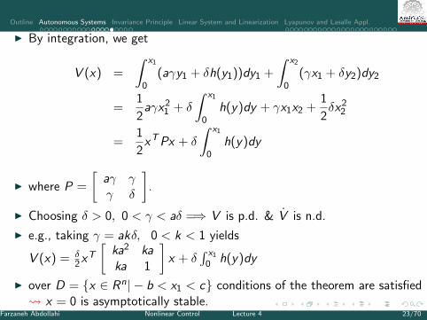
I By integration, we get
V (x) =
∫ x1
0(aγy1 + δh(y1))dy1 +
∫ x2
0(γx1 + δy2)dy2
=1
2aγx2
1 + δ
∫ x1
0h(y)dy + γx1x2 +
1
2δx2
2
=1
2xT Px + δ
∫ x1
0h(y)dy
I where P =
[aγ γγ δ
].
I Choosing δ > 0, 0 < γ < aδ =⇒ V is p.d. & V is n.d.
I e.g., taking γ = akδ, 0 < k < 1 yields
V (x) = δ2xT
[ka2 kaka 1
]x + δ
∫ x1
0 h(y)dy
I over D = x ∈ Rn| − b < x1 < c conditions of the theorem are satisfied x = 0 is asymptotically stable.
Farzaneh Abdollahi Nonlinear Control Lecture 4 23/70

Outline Autonomous Systems Invariance Principle Linear System and Linearization Lyapunov and Lasalle Appl.
Region of AttractionI For asymptotically stable Equ. pt.:
How far from the origin can the trajectory be and still converges to the origin ast −→∞ ?
I Let φ(t, x) be the sol. of x = f (x) starting at x0.Then, the Region of Attraction (RoA) is defined asthe set of all pts. x s.t. lim
t−→∞φ(t, x) = 0
I Lyap. fcn can be used to estimate the RoA:I If there is a Lyap. fcn. satisfying asymptotic stability over domain D,I and set Ωc = x ∈ Rn|V (x) ≤ c is bounded and contained in DI ∴ all trajectories starting in Ωc remains there and converges to 0 at t →∞.
I Under what condition the RoA be Rn( i.e., the Equ. pt. is globallyasymptotically stable (g.a.s))?
I the conditions of stability theory must hold globally, i.e. D = Rn.I This not enough!I for large c , the set Ωc should be kept bounded.
i.e., reduction of V (x) should also result in reduction of ‖x‖.Farzaneh Abdollahi Nonlinear Control Lecture 4 24/70

Outline Autonomous Systems Invariance Principle Linear System and Linearization Lyapunov and Lasalle Appl.
Region of AttractionI Example: V (x) =
x21
1+x21
+ x22
I It’s clear that V (x) can get smaller, but x grows unboundedly
I Babashin-Krasovskii Theorem: Let x = 0 be an Equ. pt. of x = f (x).Let V : Rn −→ R be a continuously differentiable fcn. s.t.:
I V (0) = 0I V (x) > 0, ∀x 6= 0I ‖x‖ −→ ∞ =⇒ V (x) −→∞ (i.e. it is radially unbounded)I V < 0, ∀x 6= 0
then x = 0 is globally asymptotically stableFarzaneh Abdollahi Nonlinear Control Lecture 4 25/70

Outline Autonomous Systems Invariance Principle Linear System and Linearization Lyapunov and Lasalle Appl.
Example 6 : Globally Asymptotically Stable
I Reconsider Example 5 ( h(0) = 0, xh(x) > 0, ∀x 6= 0, x ∈ (−a, a))I but assume that xh(x) > 0 hold for all x 6= 0.
I The Lyap. fcn:
V (x) =δ
2xT
[ka2 kaka 1
]x + δ
∫ x1
0
h(y)dy
is p.d. ∀x ∈ R2
I V (x) is radially unbounded.I V = −aδ(1− k)x2
2 − akδx1h(x1) < 0, ∀x ∈ R2
I ∴ origin is g.a.s.
I Important: Since the origin is g.a.s., then it must be the unique Equ.pt. of the system
I g.a.s. is not satisfied for multiple Equ. pt. problem such as pendulum.
Farzaneh Abdollahi Nonlinear Control Lecture 4 26/70

Outline Autonomous Systems Invariance Principle Linear System and Linearization Lyapunov and Lasalle Appl.
Instability TheoremI Chetaev’s Theorem Let x = 0 be an Equ. pt. of x = f (x). Let V : D −→ R
be a continuously differentiable fcn such that V (0) = 0 and V (x0) > 0 for somex0 with arbitrary small ‖x0‖. Define a set ν = x ∈ Br |V (x) > 0 whereBr = x ∈ Rn|‖x‖ < r and suppose that V (x) is p.d. in ν. Then, x = 0 isunstable.
I Example:x1 = x1 + g1(x)
x2 = −x2 + g2(x)
where |gi (x)| ≤ k‖x‖22 in a neighborhood D of originI The inequality implies, gi (0) = 0 =⇒ origin is an Equ. pt.
I Consider: V (x) = 12 (x2
1 − x22 )
I On the line x2 = 0,V (x) > 0.I V (x) = x2
1 + x22 + x1g1(x)− x2g2(x)
I Since |x1g1(x)− x2g2(x)| ≤2∑
i=1
|xi ||gi (x)| ≤ 2k‖x‖32
I ∴ V (x) ≥ ‖x‖22 − 2k‖x‖32 = ‖x‖22(1− 2k‖x‖2)I Choosing r s.t. Br ⊂ D and r < 1
2k =⇒ origin is unstable.Farzaneh Abdollahi Nonlinear Control Lecture 4 27/70

Outline Autonomous Systems Invariance Principle Linear System and Linearization Lyapunov and Lasalle Appl.
Invariance PrincipleI Recall the pendulum example:
x1 = x2
x2 =−g
lsinx1 −
k
mx2
V (x) = −km x2
2 which is n.s.d.I ∴ Lyap. theorem shows only stability. However,
I V is negative everywhere except at x2 = 0 where V = 0.I To get V = 0, the trajectory must be confined to x2 = 0I Now, from the model x2(t) ≡ 0 =⇒ x1 ≡ 0 =⇒ x1(t) = cte and
x2(t) ≡ 0 =⇒ x2 ≡ 0 =⇒ sinx1 ≡ 0I Hence, on the segment −π < x1 < π of x2 = 0 line, the system can
maintain V = 0 only at x = 0.
I Therefore, V (x) decrease to zero and x(t) −→ 0 as t −→∞.
I The idea follows from LaSalle’s Invariance PrincipleFarzaneh Abdollahi Nonlinear Control Lecture 4 28/70

Outline Autonomous Systems Invariance Principle Linear System and Linearization Lyapunov and Lasalle Appl.
Invariance Principle
I A set M is said to be a positively invariant set with respect to x = f (x),if x(0) ∈ M =⇒ x(t) ∈ M, ∀t ≥ 0
I If a solution belongs to M at some time instant, then it belongs to M forall future time.
I ∴ Equ. points and limit cycle are invariant sets
I Also the set Ω = x ∈ Rn|V (x) ≤ c with V ≤ 0 ∀x ∈ Ω is a positivelyinvariant set.
Farzaneh Abdollahi Nonlinear Control Lecture 4 29/70

Outline Autonomous Systems Invariance Principle Linear System and Linearization Lyapunov and Lasalle Appl.
Lasalle’s Theorem:I Let Ω be a compact set with property that every solution of x = f (x)
starting in Ω remains in Ω for all future time.I Let V : Ω −→ R be a continuously differentiable fcn s.t. V (x) ≤ 0 in Ω.I Let E be the set of all pts in Ω where V (x) = 0I Let M be the largest invariant set in E .
Then, every sol. starting in Ω approaches M as t −→∞I Unlike Lyap. theorem, Lasalle’s theorem does not require V (x) to be p.dI Only Ω should be bounded
I If V is p.d. ⇒ Ω = x ∈ Rn|V (x) ≤ c is bounded for suff. small cI If V is radially unbounded ⇒ Ω is bounded for all c no matter V is p.d. or
not
I To show a.s. of the origin −→ show largest invariant set in E is theorigin.
I ∴ Show that no solution can stay forever in E other than x = 0.
Farzaneh Abdollahi Nonlinear Control Lecture 4 30/70

Outline Autonomous Systems Invariance Principle Linear System and Linearization Lyapunov and Lasalle Appl.
Lasalle’s Theorem:
Farzaneh Abdollahi Nonlinear Control Lecture 4 31/70

Outline Autonomous Systems Invariance Principle Linear System and Linearization Lyapunov and Lasalle Appl.
Barbashin and Krasovskii Corollaries
I Corollary 1: Let x = 0 be an Equ. pt of x = f (x). Let V : D → R be acontinuously differentiable p.d. fcn on a domain D containing the originx = 0, s.t. V (x) ≤ 0 in D. Let S = x ∈ D|V = 0 and suppose that nosolution can stay identically in S, other than the trivial solution x(t) = 0.Then, the origin is a.s.
I Corollary 2: Let x = 0 be an Equ. pt. of x = f (x). Let V : Rn −→ Rbe a continuously differentiable, radially unbounded, p.d. fcn s.t.V (x) ≤ 0 ∀x ∈ Rn. Let S = x ∈ Rn|V = 0 and suppose that nosolution can stay in S forever except x = 0. Then, the origin is g.a.s.
Farzaneh Abdollahi Nonlinear Control Lecture 4 32/70
Outline Autonomous Systems Invariance Principle Linear System and Linearization Lyapunov and Lasalle Appl.
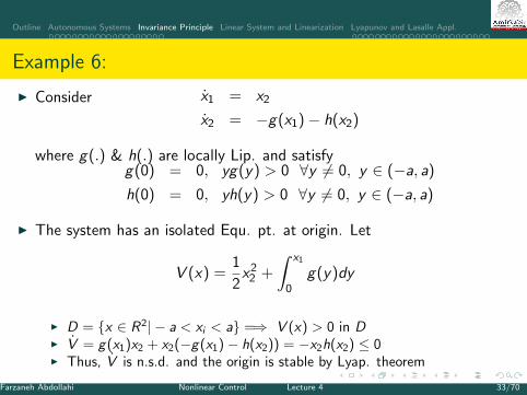
Example 6:
I Consider x1 = x2
x2 = −g(x1)− h(x2)
where g(.) & h(.) are locally Lip. and satisfyg(0) = 0, yg(y) > 0 ∀y 6= 0, y ∈ (−a, a)
h(0) = 0, yh(y) > 0 ∀y 6= 0, y ∈ (−a, a)
I The system has an isolated Equ. pt. at origin. Let
V (x) =1
2x22 +
∫ x1
0g(y)dy
I D = x ∈ R2| − a < xi < a =⇒ V (x) > 0 in DI V = g(x1)x2 + x2(−g(x1)− h(x2)) = −x2h(x2) ≤ 0I Thus, V is n.s.d. and the origin is stable by Lyap. theorem
Farzaneh Abdollahi Nonlinear Control Lecture 4 33/70

Outline Autonomous Systems Invariance Principle Linear System and Linearization Lyapunov and Lasalle Appl.
Example 6:
I Using Lasalle’s theorem, define S = x ∈ D|V = 0I V = 0 =⇒ x2h(x2) = 0 =⇒ x2 = 0, since −a < x2 < aI Hence S = x ∈ D|x2 = 0. Suppose x(t) is a traj. ∈ S ∀tI ∴ x2(t) ≡ 0 =⇒ x1 ≡ 0 =⇒ x1(t) = c , where c ∈ (−a, a). Also
x2(t) ≡ 0 =⇒ x2 ≡ 0 =⇒ g(c) = 0 =⇒ c = 0
I ∴ Only solution that can stay in S ∀ t ≥ 0 is the origin =⇒ x = 0 is a.s.
I Now, Let a =∞ and assume g satisfy:∫ y
0g(z)dz −→∞ as |y | −→ ∞.
I The Lyap. fcn V (x) = 12x2
2 +∫ x1
0 g(y)dy is radially unbounded.
I V ≤ 0 in R2 and note that S = x ∈ R2|V = 0 = x ∈ R2|x2 = 0contains no solution other than origin =⇒ x = 0 is g.a.s.
Farzaneh Abdollahi Nonlinear Control Lecture 4 34/70

Outline Autonomous Systems Invariance Principle Linear System and Linearization Lyapunov and Lasalle Appl.
Summary
I Lyapunov Direct Method:The origin of an autonomous system x = f (x)is stable if there is a continuously differentiable, p.d. function V (x) s.t.
V (x) is n.s.d., and] is asymptotically if V (x) is n.d.I V (x) is p.d./p.s.d. iff λiP > 0/λiP ≥ 0 iff all leading principle minors
of P are positive / non-negative.I Variable Gradient Method: To find a Lyap fcn: Choose g(x) s.t.
1. ∂gi∂xj
=∂gj
∂xi
2. gT (x)f (x) is n.d. (n.s.d)3. V (x) =∫ x1
0g1(y1, 0, ..., 0)dy1 +
∫ x2
0g2(x1, y2, 0, ..., 0)dy2 + ...+
∫ xn
0gn(x1, x2, ..., yn)dyn
is P.d.
I Babashin-Krasovskii Theorem: Let x = 0 be an Equ. pt. of x = f (x).Let V : Rn −→ R be a continuously differentiable fcn. s.t.: V (0) = 0,V (x) > 0, ∀x 6= 0, ‖x‖ −→ ∞ =⇒ V (x) −→∞ (i.e. it is radiallyunbounded), V < 0, ∀x 6= 0 then x = 0 is globally asymptotically stable
Farzaneh Abdollahi Nonlinear Control Lecture 4 35/70

Outline Autonomous Systems Invariance Principle Linear System and Linearization Lyapunov and Lasalle Appl.
Summary
I Another method for study a.s is defined based on Lasalle Theorem:I Corollary 1: Let x = 0 be an Equ. pt of x = f (x). Let V : D → R be a
continuously differentiable p.d. fcn on a domain D containing the originx = 0, s.t. V (x) ≤ 0 in D.Let S = x ∈ D|V = 0 and suppose that nosolution can stay identically in S, other than the trivial solution x(t) = 0.Then, the origin is a.s.
I The origin is g.a.s. if D = Rn, and V (x) is radially unbounded.
Farzaneh Abdollahi Nonlinear Control Lecture 4 36/70

Outline Autonomous Systems Invariance Principle Linear System and Linearization Lyapunov and Lasalle Appl.
Invariance Principle
I Lasalle’s theorem can also extend the Lyap. theorem in three differentdirections
1. It gives an estimate of the RoA not necessarily in the form ofΩc = x ∈ Rn| V (x) ≤ c. The set can be any positively invariant setwhich leads to less conservative estimate.
2. Can determine stability of Equ. set, rather than isolated Equ. pts.3. The function V (x) does not have to be positive definite.
I Example 7: shows how to use Lasalle’s theorem for system with Equ.sets rather than isolated Equ. pts
I A simple adaptive control problem:
x = ax + u a unknown
with the adaptive control law
u = −kx ; k = γx2, γ > 0
Farzaneh Abdollahi Nonlinear Control Lecture 4 37/70

Outline Autonomous Systems Invariance Principle Linear System and Linearization Lyapunov and Lasalle Appl.
Example 7:I Let x1 = x , x2 = k , we get:
x1 = −(x2 − a)x1
x2 = γx21
I The line x1 = 0 is an Equ. setI Show that the traj. of closed-loop system approaches this set as t −→ ∞
I i.e. the adaptive system regulates y to zero (x1 −→ 0 as t −→ ∞).
I Consider the Lyap. fcn candidate:
V (x) =1
2x21 +
1
2γ(x2 − b)2
where b > a.I V = −x2
1 (b − a) ≤ 0I The set Ω = x ∈ Rn|V (x) ≤ c is a compact positively invariant set
Farzaneh Abdollahi Nonlinear Control Lecture 4 38/70

Outline Autonomous Systems Invariance Principle Linear System and Linearization Lyapunov and Lasalle Appl.
Example 7:I V (x) is radially unbounded =⇒ Lasalle’s theorem conditions are satisfied
with the set E as E = x ∈ Ω|x1 = 0
I Since any pt on x1 = 0 line is an Equ. pt, E is an invariant set: M = E .
I Hence, every trajectory starting in Ω approaches E as t −→ ∞, i.e.x1(t) −→ 0 as t −→ ∞.
I V is radially unbounded =⇒ the result is global
I Note that in the above example the Lyapunov function depends on aconstant b which is required to satisfy b > a
I But it is not known we may not know the constant b explicitly, but weknow that it always exists.
I This highlights another feature of Lyapunov’s method:I In some situations, we may be able to assert the existence of a Lyapunov
function that satisfies the conditions, even though we may not explicitlyknow that function.
Farzaneh Abdollahi Nonlinear Control Lecture 4 39/70

Outline Autonomous Systems Invariance Principle Linear System and Linearization Lyapunov and Lasalle Appl.
Linear System and Linearization
I Given x = Ax , the Equ. pt. is at origin
I It is isolated iff det A 6= 0,
I System has an Equ. subspace if det A = 0, the subspace is the nullspace of A.
I The linear system cannot have multiple isolated Equ. pt. sinceI Linearity requires that if x1 and x2 are Equ. pts., then all pts. on the line
connecting them should also be Equ. pts.
I Theorem: The Equ. pt. x = 0 of x = Ax is stable iff all eigenvalues ofA satisfy Reλi ≤ 0 and every eigenvalue with Reλi = 0 and algebricmultiplicity qi ≥ 2, rank(A− λi I ) = n − qi , where n is dimension of x.The Equ. pt. x = 0 is globally asymptotically stable iff Reλi < 0.
Farzaneh Abdollahi Nonlinear Control Lecture 4 40/70

Outline Autonomous Systems Invariance Principle Linear System and Linearization Lyapunov and Lasalle Appl.
Linear Systems and Linearization
I When all eigenvalues of A satisfy Reλi < 0, A is called a Hurwitz matrix.I Asymptotic stability can be verified by using Lyapunov’s method :
I Consider a quadratic Lyap. fcn candidate:
V (x) = xT P x , P = PT > 0
V = xT Px + xT Px , xT (AT P + PA)x , −xT Q x
where
AT P + P A = −Q, Q = QT Lyapunov Equation
I If Q is p.d., then we conclude that x = 0 is g.a.s.I We can proceed alternatively as follows:I Start by choosing Q = QT , Q > 0, then solve the Lyap. eqn. for P.I If P > 0, then x = 0 is g.a.s.
Farzaneh Abdollahi Nonlinear Control Lecture 4 41/70

Outline Autonomous Systems Invariance Principle Linear System and Linearization Lyapunov and Lasalle Appl.
Linear Systems and LinearizationI Theorem: A matrix A is a stable matrix, i.e. Re λi < 0 iff for every
given Q = QT > 0, ∃ P = PT > 0 that satisfies the Lyap. eq.Moreover, if A is a stable matrix, then P is unique.
I Example 8:A =
[0 −11 −1
]
I Let Q =
[1 00 1
]= QT > 0
I denote P =
[P11 P12
P12 P22
]= PT > 0
I The Lyap. eq. AT P + P A = −Q becomes
2 P12 = −1
−P11 − P12 + P22 = 0
−2 P12 − 2P22 = −1
Farzaneh Abdollahi Nonlinear Control Lecture 4 42/70
Outline Autonomous Systems Invariance Principle Linear System and Linearization Lyapunov and Lasalle Appl.
Linear Systems and Linearization
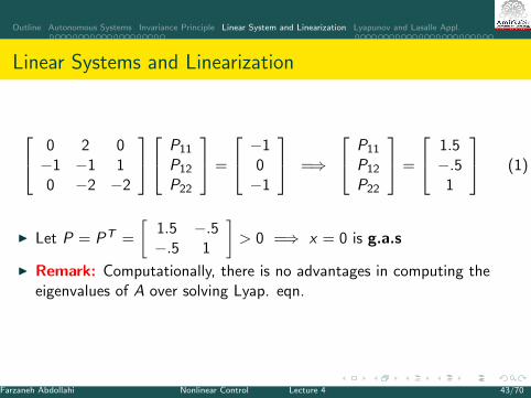
0 2 0−1 −1 10 −2 −2
P11
P12
P22
=
−10−1
=⇒
P11
P12
P22
=
1.5−.5
1
(1)
I Let P = PT =
[1.5 −.5−.5 1
]> 0 =⇒ x = 0 is g.a.s
I Remark: Computationally, there is no advantages in computing theeigenvalues of A over solving Lyap. eqn.
Farzaneh Abdollahi Nonlinear Control Lecture 4 43/70

Outline Autonomous Systems Invariance Principle Linear System and Linearization Lyapunov and Lasalle Appl.
Linear Systems and Linearization
I Consider x = f (x) where f : D −→ Rn, D ⊂ Rn, is continuously diff. Letx = 0 is in the interior of D and f (0) = 0.
I In a small neighborhood of x = 0, the nonlinear system x = f (x) can belinearized by x = Ax .
I Proof: Ref. Khalil’s book
I Theorem (Lyapunov’s First Method):I Let x = 0 be an Equ. pt. for x = f (x) where f : D −→ Rn is
continuously differentiable and D is a nghd of origin. Let A = ∂f∂x
∣∣x=0
,then
1. x = 0 is a.s. if Reλi < 0, i = 1, ..., n2. x = 0 is unstable if Reλi > 0, for one or more eigenvalues
Farzaneh Abdollahi Nonlinear Control Lecture 4 44/70

Outline Autonomous Systems Invariance Principle Linear System and Linearization Lyapunov and Lasalle Appl.
Linear Systems and LinearizationI Example 9: x = ax3
I Linearization about x = 0 yields:
A =∂f
∂x
∣∣∣∣x=0
= 3ax2∣∣x=0
= 0
I Linearization fails to determine stabilityI If a < 0, x = 0 is a.s.I To see this, let V (x) = x4 =⇒ V = 4x3x = 4ax6
I If a > 0, x = 0 is unstableI If a ≤ 0, x = 0 is stable, starting at any x , remains in x
I Example 10:
x1 = x2
x2 = −(g
l
)sin x1 −
(k
mx2
)Farzaneh Abdollahi Nonlinear Control Lecture 4 45/70

Outline Autonomous Systems Invariance Principle Linear System and Linearization Lyapunov and Lasalle Appl.
Linear Systems and LinearizationI Linearization about 2 Equ. pts. (0, 0) & (π, 0):
A =∂f
∂x=
[∂f1∂x1
∂f1∂x2
∂f2∂x1
∂f2∂x2
]=
[0 1
−gl cos x1 − k
m
]I At (0, 0)
I A =
[0 1− g
l − km
], λ1,2 = − 1
2km ±
12
√( k
m )2 − 4 gl
I ∴ ∀g , k , l ,m > 0 =⇒ Re(λ1, λ2) < 0 =⇒ x = 0 is a.s.I If k = 0 =⇒ Re(λ1, λ2) = 0 =⇒ eigenvalues on jω axis,rank(A−λi I ) 6= 0∴ stability cannot be determined.
I At (π, 0) , change the variable to z1 = x1 − π, z2 = x2
I A =
[0 1gl − k
m
], λ1,2 = − 1
2km ±
12
√( k
m )2 + 4 gl
I ∴ ∀g , k , l ,m > 0 =⇒ there is one eigenvalue in the open right-half plane=⇒ x = 0 is unstable.
Farzaneh Abdollahi Nonlinear Control Lecture 4 46/70

Outline Autonomous Systems Invariance Principle Linear System and Linearization Lyapunov and Lasalle Appl.
Example: Robot ManipulatorI Dynamics:
M(q)q + C (q, q)q + Bq + g(q) = u (2)
where M(q) is the n × n inertia matrix of the manipulator
I C (q, q)q is the vector of Coriolis and centrifugal forces
I g(q) is the term due to the Gravity
I Bq is the viscous damping term
I u is the input torque, usually provided by a DC motor
I Objective: To regulate the joint position q around desired position qd .
I A common control strategy PD+Gravity:
u = KP q− KD q + g(q)
where q = qd − q is the error between the desired and actual position
I KP and KD are diagonal positive proportional and derivative gains.Farzaneh Abdollahi Nonlinear Control Lecture 4 47/70

Outline Autonomous Systems Invariance Principle Linear System and Linearization Lyapunov and Lasalle Appl.
Example: Robot ManipulatorI Consider the following Lyap. fcn candidate:
V =1
2qT M(q)q +
1
2qT KP q
I The first term is the kinetic energy of the robot and the second termaccounts for “artificial potential energy” associated with virtual spring inPD control law (proportional feedback Kpq)
I Physical properties of a robot manipulator:
1. The inertia matrix M(q) is positive definite2. The matrix M(q)− 2C(q, q) is skew symmetric
I V is positive in Rn except at the goal position q = qd , q = 0
V = qT M(q)q +1
2qT M(q)q− qT KP q
I Substituting M(q)q from (2) into the above equation yields
V = qT (u − C (q, q)q− Bq− g(q)) +1
2qT M(q)q− qT KP q
= qT (u − Bq− KP q− g(q)) +1
2qT (M(q)− 2C (q, q))q
Farzaneh Abdollahi Nonlinear Control Lecture 4 48/70
Outline Autonomous Systems Invariance Principle Linear System and Linearization Lyapunov and Lasalle Appl.
Example: Robot Manipulator
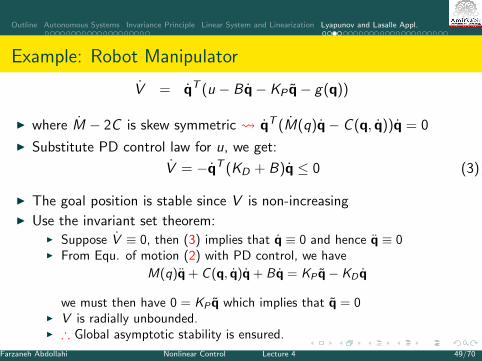
V = qT (u − Bq− KP q− g(q))
I where M − 2C is skew symmetric qT (M(q)q− C (q, q))q = 0
I Substitute PD control law for u, we get:
V = −qT (KD + B)q ≤ 0 (3)
I The goal position is stable since V is non-increasingI Use the invariant set theorem:
I Suppose V ≡ 0, then (3) implies that q ≡ 0 and hence q ≡ 0I From Equ. of motion (2) with PD control, we have
M(q)q + C (q, q)q + Bq = KP q− KD q
we must then have 0 = KP q which implies that q = 0I V is radially unbounded.I ∴ Global asymptotic stability is ensured.
Farzaneh Abdollahi Nonlinear Control Lecture 4 49/70

Outline Autonomous Systems Invariance Principle Linear System and Linearization Lyapunov and Lasalle Appl.
Example: Robot Manipulator
I In case, the gravitational terms is not canceled, V is modified to:
V = −qT ((KD + B)q + g(q))
I The presence of gravitational term means PD control alone cannotguarantee asymptotic tracking.
I Assuming that the closed loop system is stable, the robot configuration qwill satisfy
KP(qd − q) = g(q)
I The physical interpretation of the above equation is that:I The configuration q must be such that the motor generates a steady state
“holding torque” KP(qd − q) sufficient to balance the gravitational torqueg(q).
I ∴ the steady state error can be reduced by increasing KP .
Farzaneh Abdollahi Nonlinear Control Lecture 4 50/70

Outline Autonomous Systems Invariance Principle Linear System and Linearization Lyapunov and Lasalle Appl.
Control Design Based on Lyapunov’s Direct Method
I Basically there are two approaches to design control usingLyapunov’s direct method
I Choose a control law, then find a Lyap. fcn to justify thechoice
I Candidate a Lyap. fcn, then find a control law to satisfy theLyap. stability conditions.
I Both methods have a trial and error flavorI In robot manipulator example the first approach was applied:
I First a PD controller was chosen based on physical intuitionI Then a Lyap. fcn. is found to show g.a.s.
Farzaneh Abdollahi Nonlinear Control Lecture 4 51/70

Outline Autonomous Systems Invariance Principle Linear System and Linearization Lyapunov and Lasalle Appl.
Control Design Based on Lyapunov’s Direct MethodI Example: Regulator Design
I Consider the problem of stabilizing the system:x − x3 + x2 = u
I In other word, make the origin an asymptotically stable Equ. pt.
I Recall the example: x1 = x2
x2 = −g(x1)− h(x2)
where g(.) & h(.) are locally Lip. and satisfyg(0) = 0, yg(y) > 0 ∀y 6= 0, y ∈ (−a, a)
h(0) = 0, yh(y) > 0 ∀y 6= 0, y ∈ (−a, a)
I Asymptotic stability of such system could be shown by selecting thefollowing Lyap. fcn:
V (x) =1
2x22 +
∫ x1
0g(y)dy
Farzaneh Abdollahi Nonlinear Control Lecture 4 52/70
Outline Autonomous Systems Invariance Principle Linear System and Linearization Lyapunov and Lasalle Appl.
Example: Regulator DesignI Let x1 = x , x2 = x . The above example motivates us to select the
control law u asu = u1(x) + u2(x)
where
x(x3 + u1(x)) < 0 for x 6= 0
x(u2(x)− x2) < 0 for x 6= 0
I The globally stabilizing controller can be designed even in the presence ofsome uncertainties on the dynamics:
x + α1x3 + α2x2 = u
where α1 and α2 are unknown, but s.t. α1 > − 2 and |α2| < 5
I This system can be globally stabilized using the control law:u = −2x3 − 5(x + x3)
Farzaneh Abdollahi Nonlinear Control Lecture 4 53/70
Outline Autonomous Systems Invariance Principle Linear System and Linearization Lyapunov and Lasalle Appl.
Estimating Region of Attraction
I Sometimes just knowing a system is a.s. is not enough. At least anestimation of RoA is required.
I Example: Occurring fault and finding ”critical clearance time”
I Let x = 0 be an Equ. pt. of x = f (x). Let φ(t, x) be the sol starting at xat time t=0. The Region Of Attraction (RoA) of the origin denoted byRA is defined by:
RA = x ∈ Rn|φ(t, x) −→ 0 as t −→ ∞
I Lemma: If x = 0 is an a.s. Equ. pt. of x = f (x), then its RoA RA is anopen, connected, invariant set. Moreover, the boundary of RoA, ∂RA, isformed by trajectories of x = f (x).
I ∴ one way to determine RoA is to characterize those trajectories that lieon ∂RA.
Farzaneh Abdollahi Nonlinear Control Lecture 4 54/70

Outline Autonomous Systems Invariance Principle Linear System and Linearization Lyapunov and Lasalle Appl.
Example: Van-der-Pol
I Dynamics of oscillator in reverse time
x1 = −x2
x2 = x1 + (x21 − 1)x2
I The system has an Equ. pt at origin and an unstable limit cycle.
I The origin is a stable focus −→ it is a.s.Farzaneh Abdollahi Nonlinear Control Lecture 4 55/70
Outline Autonomous Systems Invariance Principle Linear System and Linearization Lyapunov and Lasalle Appl.
Example: Van-der-Pol
I Checking by linearizaton method
A =∂f
∂x
∣∣∣∣x=0
[0 −11 −1
]I λ = −1/2± j
√3/2 Re λi < 0
I Clearly, RoA is bounded since trajectories outside the limit cycle driftaway from it
I ∴ ∂RA is the limit cycle
Farzaneh Abdollahi Nonlinear Control Lecture 4 56/70
Outline Autonomous Systems Invariance Principle Linear System and Linearization Lyapunov and Lasalle Appl.
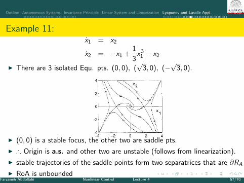
Example 11:x1 = x2
x2 = −x1 +1
3x31 − x2
I There are 3 isolated Equ. pts. (0, 0), (√
3, 0), (−√
3, 0).
I (0, 0) is a stable focus, the other two are saddle pts.
I ∴ Origin is a.s. and other two are unstable (follows from linearization).
I stable trajectories of the saddle points form two separatrices that are ∂RA
I RoA is unboundedFarzaneh Abdollahi Nonlinear Control Lecture 4 57/70

Outline Autonomous Systems Invariance Principle Linear System and Linearization Lyapunov and Lasalle Appl.
Example 11:I Recall the example:
x1 = x2
x2 = −h(x1)− ax2
V =δ
2xT
[ka2 kaka 1
]x + δ
∫ x1
0hdy
I Let
V = 12xT
[12
12
12 1
]x +
∫ x1
0
(y − 1
3y3)
dy
=34x2
1 − 112x4
1 + 12x1x2 + 1
2x22
I We get: V = −12x2
1
(1− 1
3x21
)− 1
2x22
I Define D = x ∈ R2| −√
3 < x1 <√
3I ∴ V (x) > 0 and V (x) < 0 in D − 0,I From the phase portrait =⇒ D is not a
subset of RA. Tell me why?!!Farzaneh Abdollahi Nonlinear Control Lecture 4 58/70

Outline Autonomous Systems Invariance Principle Linear System and Linearization Lyapunov and Lasalle Appl.
Estimating RoAI Traj starting in D move from one Lyap. surface to V (x) = c1 to an inner
surface V (x) = c2 with c2 < c1.
I However, there is no guarantee that the traj. will remain in D forever.
I Once, the traj leaves D, no guarantee that V remains negative.
I This problem does not occur in RA since RA is an invariant set.
I The simplest estimate is given by the set
Ωc = x ∈ Rn|V (x) ≤ c
where Ωc isbounded and connected and Ωc ∈ DI Note that V (x) ≤ c may have more than one component, only the
bounded component which belong to D is acceptable.I Example: If V (x) = x2/(1 + x4).and D = |x | < 1I The set V (x) ≤ 1/4 has two components |x | ≤
√2−√
3 and
|x | ≤√
2 +√
3 only |x | ≤√
2−√
3 is acceptable.
Farzaneh Abdollahi Nonlinear Control Lecture 4 59/70

Outline Autonomous Systems Invariance Principle Linear System and Linearization Lyapunov and Lasalle Appl.
Estimating RoAI To find RoA, first we need to find a domain D in which V is n.d.
I Then, a bounded set Ωc ⊂ D shall be sought
I We are interested in largest set Ωc , i.e. the largest value of c since Ωc isan estimate of RA.
I V is p.d. everywhere in R2.
I If V (x) = xT Px , let D = x ∈ R2| ‖x‖ ≤ r. Once, D is obtained,then select Ωc ⊂ D by c < min
‖x‖=rV (x)
I In words, the smallest V (x) = c which fits into D.
I SincexT Px ≥ λmin(P)‖x‖2
I We can choosec < λmin(P)r2
I To enlarge the estimate of RA =⇒ find largest ball on which V is n.d.Farzaneh Abdollahi Nonlinear Control Lecture 4 60/70

Outline Autonomous Systems Invariance Principle Linear System and Linearization Lyapunov and Lasalle Appl.
Example 12:
x1 = −x2
x2 = x1 + (x21 − 1)x2
I From the linearization ∂f∂x
∣∣x=0
=
[0 −11 −1
]is stable
I Taking Q = I and solve the Lyap. equation:
PA + AT P = −I =⇒ P =
[1.5 −.5−.5 1
]I λmin(P) = 0.69
I V = −(x21 + x2
2 )− (x31 x2 − 2x2
1 x22 ) ≤ −‖x‖22 + |x1||x1x2||x1 − 2x2| ≤
−‖x‖22 +√
52 ‖x‖
42
I where |x1| ≤ ‖x‖2, |x1x2| ≤ ‖x‖22/2, |x1− 2x2| ≤√
5‖x‖2I V is n.d. on a ball D of radius
r2 = 2/√
5 = 0.894 c < 0.894× 0.69 = 0.617Farzaneh Abdollahi Nonlinear Control Lecture 4 61/70

Outline Autonomous Systems Invariance Principle Linear System and Linearization Lyapunov and Lasalle Appl.
Example 12:
I To find less conservative estimate of Ωc :
I Let x1 = ρ cosθ, x2 = ρ sinθ
V = −ρ2 + ρ4cos2θsinθ (2sinθ − cosθ)
≤ −ρ2 + ρ4∣∣cos2θsinθ
∣∣ |2sinθ − cosθ|≤ −ρ2 + ρ4(.3849)(2.2361)
≤ −ρ2 + .861ρ4 < 0 for ρ2 <1
.861
I c = .8 < .69.861 = .801
I Thus the set:Ωc = x ∈ R2| V (x) ≤ .8 is an estimate of RA.
Farzaneh Abdollahi Nonlinear Control Lecture 4 62/70

Outline Autonomous Systems Invariance Principle Linear System and Linearization Lyapunov and Lasalle Appl.
Example 12:I A lesser conservative estimation of RoA:
I plot the contour of V = 0I plot V (x) = c for increasing c to find largest c where V < 0
I The c obtained by this method is c = 2.25.
Farzaneh Abdollahi Nonlinear Control Lecture 4 63/70

Outline Autonomous Systems Invariance Principle Linear System and Linearization Lyapunov and Lasalle Appl.
Example 13:x1 = −2x1 + x1x2
x2 = −x2 + x1x2
I There are two Equ. pts., (0, 0), (1, 2).
I At (1, 2) A =
[0 −12 0
]=⇒ unstable
(λ1,2 = ±
√2)
(saddle pt.)
I At (0, 0) A =
[−2 00 −1
]=⇒ a.s.
I Taking Q = I and solving Lyap Eq. AT P + PA = −I⇒P =
[14 00 1
2
]I ∴ The Lyap. fcn is V (x) = xT Px
I We have V = −(x21 + x2
2 ) + 12(x2
1 x2 + 2x1x22 )
I Find largest D s.t.V is n.d. in D.
I Let x1 = ρ cosθ, x2 = ρ sinθFarzaneh Abdollahi Nonlinear Control Lecture 4 64/70

Outline Autonomous Systems Invariance Principle Linear System and Linearization Lyapunov and Lasalle Appl.
Example 13:
V = −ρ2 + ρ3cosθsinθ
(sinθ +
1
2cosθ
)≤ −ρ2 +
1
2ρ3 |sin2θ|
∣∣∣∣sinθ +1
2cosθ
∣∣∣∣≤ −ρ2 +
√5
4ρ3 < 0 for ρ <
4√5
I Since λmin(P) = 14 =⇒, we choose
c = .79 < 14 ×
(4√5
)2= .8
I Thus the set:Ωc = x ∈ R2| V (x) ≤ .79 ⊂ RA.
I Estimating RoA by the set Ωc is simple but conservative
I Alternatively Lasalle’s theorem can be used. It provides an estimate of RA
by the set Ω which is compact and positively invariant set.Farzaneh Abdollahi Nonlinear Control Lecture 4 65/70
Outline Autonomous Systems Invariance Principle Linear System and Linearization Lyapunov and Lasalle Appl.
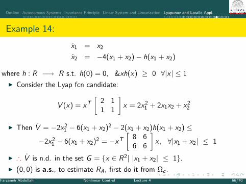
Example 14:
x1 = x2
x2 = −4(x1 + x2)− h(x1 + x2)
where h : R −→ R s.t. h(0) = 0, &xh(x) ≥ 0 ∀|x | ≤ 1
I Consider the Lyap fcn candidate:
V (x) = xT
[2 11 1
]x = 2x2
1 + 2x1x2 + x22
I Then V = −2x21 − 6(x1 + x2)2 − 2(x1 + x2)h(x1 + x2) ≤
−2x21 − 6(x1 + x2)2 = −xT
[8 66 6
]x , ∀|x1 + x2| ≤ 1
I ∴ V is n.d. in the set G = x ∈ R2| |x1 + x2| ≤ 1.I (0, 0) is a.s., to estimate RA, first do it from Ωc .
Farzaneh Abdollahi Nonlinear Control Lecture 4 66/70
Outline Autonomous Systems Invariance Principle Linear System and Linearization Lyapunov and Lasalle Appl.
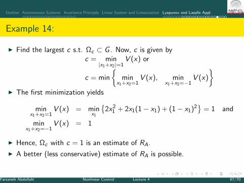
Example 14:
I Find the largest c s.t. Ωc ⊂ G . Now, c is given byc = min
|x1+x2|=1V (x) or
c = min
min
x1+x2=1V (x), min
x1+x2=−1V (x)
I The first minimization yields
minx1+x2=1
V (x) = minx1
2x2
1 + 2x1(1− x1) + (1− x1)2
= 1 and
minx1+x2=−1
V (x) = 1
I Hence, Ωc with c = 1 is an estimate of RA.
I A better (less conservative) estimate of RA is possible.
Farzaneh Abdollahi Nonlinear Control Lecture 4 67/70
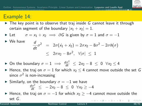
Outline Autonomous Systems Invariance Principle Linear System and Linearization Lyapunov and Lasalle Appl.
Example 14:I The key point is to observe that traj inside G cannot leave it through
certain segment of the boundary |x1 + x2| = 1.
I Let σ = x1 + x2 =⇒ ∂G is given by σ = 1 and σ = −1
I We have d
dtσ2 = 2σ(x1 + x2) = 2σx2 − 8σ2 − 2σh(σ)
≤ 2σx2 − 8σ2, ∀|σ| ≤ 1
I On the boundary σ = 1 =⇒ dσ2
dt ≤ 2x2 − 8 ≤ 0 ∀x2 ≤ 4
I Hence, the traj on σ = 1 for which x2 ≤ 4 cannot move outside the set Gsince σ2 is non-increasing
I Similarly, on the boundary σ = −1 we havedσ2
dt ≤ − 2x2 − 8 ≤ 0 ∀x2 ≥ −4
I Hence, the traj on σ = −1 for which x2 ≥ −4 cannot move outside theset G .
Farzaneh Abdollahi Nonlinear Control Lecture 4 68/70

Outline Autonomous Systems Invariance Principle Linear System and Linearization Lyapunov and Lasalle Appl.
Example 14:
I To define the boundary of G , we need to find two other segments to closethe set.
I We can take them as the segments of Lyap. fcn surface
I Let c1 be s.t. V (x) = c1 intersects the boundary of x1 + x2 = 1 at x2 = 4and let c2 be s.t. V (x) = c2 intersects the boundary of x1 + x2 = −1 atx2 = −4
I Then, we define V (x) = min c1, c2, we have
c1 = V (x)|x1 = −3x2 = 4
= 10 &c2 = V (x)|x1 = 3
x2 = −4
= 10
Farzaneh Abdollahi Nonlinear Control Lecture 4 69/70

Outline Autonomous Systems Invariance Principle Linear System and Linearization Lyapunov and Lasalle Appl.
Example 14:I The set Ω is defined by
Ω = x ∈ R2|V (x) ≤ 10 &|x1 + x2| ≤ 1
I This set is closed and bounded and positively invariant. Also, V is n.d.in Ω since Ω ⊂ G =⇒ Ω ⊂ RA.
Farzaneh Abdollahi Nonlinear Control Lecture 4 70/70