nonlinear nonmodal stability theory - damtp.cam.ac.uk · the reference state deep within the basin...

Nonlinear NonmodalStability Theory

R. R. Kerswell,School of Mathematics, Bristol University, Bristol, U.K., BS8 1TW; email:

[email protected]

Xxxx. Xxx. Xxx. Xxx. YYYY. AA:1–30

This article’s doi:

10.1146/((please add article doi))

Copyright c© YYYY by Annual Reviews.

All rights reserved

Keywords

transition, optimization, energy growth, nonlinear stability

Abstract

This review discusses a recently developed optimization technique for

analysing the nonlinear stability of a flow state. It is based upon a

nonlinear extension of nonmodal analysis and, in its simplest form,

consists of finding the disturbance to the flow state of a given amplitude

which experiences the largest energy growth at a certain time later.

When coupled with a search over the disturbance amplitude, this can

reveal the disturbance of least amplitude - called the ‘minimal seed’

- for transition to turbulence. The approach bridges the theoretical

gap between (linear) nonmodal theory and the (nonlinear) dynamical

systems approach to fluid flows by providing the ability to explore phase

space a finite distance from the reference flow state. Various ongoing

and potential applications of the technique are discussed.

1

1. History and Motivation

Hydrodynamic stability theory has been of central importance in fluid mechanics ever since

the observation that the property of a flow state being a solution of the governing equations

is no guarantee that it will actually be realised in practice. Starting in the late 19th

century and stimulated by the first controlled experiments of Reynolds (1883a,b), the initial

attempts to rationalise why a flow state might be unstable centred on the idea of linear

stability analysis (Rayleigh 1880, Kelvin 1887). In this, the linearised initial value problem

describing how infinitesimal disturbances temporally evolve on top of the steady reference

state is converted into an eigenvalue problem for the (possibly complex) growth rates of

‘normal’ modes whose temporal behaviour is exponential. These growth rates reveal the

long time behaviour of the system, with just a single unstable one being enough to establish

the linear instability of the reference state. The approach works well in explaining some

experiments - for example, Rayleigh-Benard convection (Rayleigh 1916) and Taylor-Couette

flow (Taylor 1923) - but not others, with wall-bounded shear flows such as plane Couette

flow, channel flow and pipe flow being prime examples of failure.

Linear stability analysis, however, says nothing about the short-time behaviour of the

linearised initial value problem which it was realised much later could be very different

(Boberg & Brosa 1988, Farrell 1988, Gustavsson 1991, Butler & Farrell 1992, Reddy &

Henningson 1993, Henningson & Reddy 1994, Trefethen et al. 1993; see Schmid 2007 for a

review). A new formulation was developed to analyse this behaviour - variously called ‘tran-

sient growth’ (Reddy & Henningson 1993) , ‘optimal perturbation theory’ (Butler & Farrell

1992) or ‘nonmodal analysis’ (Schmid 2007) - which started to explain the ‘hit-or-miss’ per-

formance of linear stability analysis by revealing that for flows with no predicted long-time

disturbance growth, there could nevertheless be substantial but transient short-time energy

amplification. The implication was that this energy growth could amplify a small distur-

bance into one which could trigger the transition to turbulence seen in experiments through

nonlinear processes, although the analysis was strictly only linear (substantially amplified

infinitesimal disturbances are still only infinitesimal). Interestingly, this new formulation

revolved around considering the evolution of a mixture of normal modes rather than just

one in isolation and revealed how the non-orthogonality of these modes with each other

(present when the linearised operator is non-normal) can lead to short-time energy growth.

The initial and final disturbances of the energy growth episode have very different spatial

structures - hence the term ‘non-modal’ analysis - whereas in linear stability, or ‘modal’

analysis, the normal modes maintain their spatial structure as they evolve.

Non-Normal: An

operator/matrix L is

non-normal if it doesnot commute with

its adjoint/transpose

L†, i.e. LL† 6= L†L.

Slightly after this nonmodal approach had completed the linear perspective of stability

in the early 1990s, an alternative fully nonlinear dynamical systems approach started to

emerge. This was sparked by the discovery of new finite amplitude solutions disconnected

from the reference state in shear flows (see the reviews Kerswell 2005, Eckhardt et al. 2007,

Kawahara et al. 2012) and was made feasible by the increasing availability of computational

power. In this approach, the flow is viewed as a (huge) dynamical system in which the flow

state evolves along a trajectory in a phase space populated by various invariant sets (exact

solutions) and their stable and unstable manifolds. In the case of a linearly-stable reference

state, transition or ‘nonlinear instability’ occurs when a finite disturbance to the system

puts the flow state beyond the basin of attraction of the reference state in phase space.

The dynamical systems approach to transition focuses on fully nonlinear structures like

basin boundaries and what happens beyond them whereas nonmodal analysis describes

how infinitesimal disturbances can grow temporarily in the immediate neighbourhood of

2 R. R. Kerswell

the reference state deep within the basin of attraction.

Recently a theoretical technique, which is the nonlinear extension of nonmodal analysis,

has been developed to bridge this gap in perspective and disturbance amplitude. Concep-

tually, the addition of nonlinearity to (linear) nonmodal analysis is a simple step and as a

result has been formulated independently in (at least) three different parts of the scientific

literature over the last 15 years (in transitional flows by Pringle & Kerswell 2010, Cherubini

et al. 2010 and Monokrousos et al. 2011 - see §4.1; in oceanography by Mu et al. 2004 - see

§5.1; and in thermoacoustics by Juniper 2011a - see §5.2 ). Mathematically, however, non-

linearity changes everything. What was a convex optimization problem to maximise energy

growth with a unique optimiser now becomes a fully nonlinear, non-convex optimization

problem where much less is known about the possibly multiple solutions (local as well as

global maxima) or how to find them. However, the key recent advance has been the realisa-

tion that such problems are now solvable for the 3D Navier-Stokes equation discretised by

a large number (O(105-106)) of degrees of freedom (Pringle & Kerswell 2010, Cherubini et

al. 2010, Monokrousos et al. 2011) by using a direct-adjoint looping approach on a desktop

computer. That this is a step up in computational complexity, however, is reflected in the

fact that the first nonlinear energy growth optimals incorporating the full 3D Navier-Stokes

equations were computed (Pringle & Kerswell 2010, Cherubini et al. 2010) fully 18 years

after the first 3D linear energy growth optimal (Butler & Farrell 1992).

Nonlinear Stability

The nonlinear stability of a reference state is usually couched in terms of how an energy norm E(t) (e.g.

the kinetic energy) of any disturbance to the reference state evolves in time. If limt→∞E(t)/E(0) = 0 for

all E(0) ≤ δ, where δ is finite, then the reference state is nonlinearly stable and δ measures how stable.

In its simplest form, nonlinear nonmodal analysis seeks to identify the disturbance

from among all disturbances of a given energy E(0) which optimises the energy growth,

G(E(0), T ) := E(T )/E(0), some time T later. While the result of (linear) nonmodal analysis

is recovered when E(0)→ 0, increasing E(0) explores ever more distant parts of the basin of

attraction away from the reference state. If E(0) is increased enough, the set of competing

disturbances includes initial conditions outside the basin of attraction which is reflected in a

step change in the optimal energy gain found. Determining the critical starting energy value

when this occurs identifies the finite-amplitude disturbance which first breaches the basin

boundary of the reference state. In this way nonlinear nonmodal analysis coupled with a

search over the initial energy E(0) represents a nonlinear stability analysis - called ‘nonlinear

nonmodal stability analysis’ here - since the most ‘dangerous’ disturbance which can cause

the system to evolve to another state is found together with a measure of how nonlinearly

stable the reference state is in the form of the minimal energy needed to initiate this event.

The purpose of this review is to describe the results found so far using this nonlinear

nonmodal stability analysis and to highlight the huge potential for new applications. An

earlier progress report (Kerswell et al. 2014) emphasized the generality of this approach

as a fully nonlinear optimization technique for studying nonlinear systems whereas here

the focus is on its use to probe nonlinear stability in fluid mechanics and the fact that it

is a natural extension of (linear) nonmodal stability analysis in hydrodynamic stability, as

www.annualreviews.org • Nonlinear Nonmodal Stability Theory 3

reviewed a decade ago by Schmid (2007).

2. Overview

The plan of this review is to first explain in §3 the procedure for performing nonlinear

nonmodal analysis which, in its simplest form, is the procedure of finding the optimal energy

growth over all disturbances of a given starting energy and time horizon constrained by the

3D Navier-Stokes equation for an incompressible fluid. This is the fundamental, fully-

nonlinear optimization problem which underpins everything that follows. The objective

functional to be optimised needn’t be the energy, nor must the initial amplitude constraint

also be the energy, but these simple choices are the most logical historically (nonmodal

analysis focusses on this), natural mathematically and illustrate the phenomenology most

clearly. A series of subsequent sections then outline how the results of this optimization

procedure - the optimal disturbance at one choice of the initial energy and target time -

can then be utilised in different ways to study the nonlinear stability of a linearly-stable

reference state. It is this two-tier process of nonlinear nonmodal analysis coupled to, say, a

subsequent search over the initial energy which constitutes the nonlinear nonmodal stability

theory titling this article.

The primary application so far has been in bistable systems where the disturbance of

smallest energy to trigger transition from one state (typically a steady laminar flow) to

the other (a turbulent state) is sought: see §4.1. Section 4.2 discusses the use of nonlinear

nonmodal analysis to identify different types of transition scenario, where, for example the

flow undergoes a ‘bursting’ (large energy event) before settling down to the (lower energy)

turbulent state, or rapid transition is required (turbulence is reached after a given time

rather than asymptotically long times). §4.3 then describes preliminary work directed at

identifying nearby unstable solutions to the reference state which is the only attractor in

the system. This scenario is now realised to be quite a common situation in low Reynolds

number shear flows and being able to identify when new alternative solutions appear in

phase space as the Reynolds number increases is of key importance in anticipating the

emergence of a chaotic repellor. §4.4 discusses the issue of how the analysis can be modified

to probe the nonlinear stability of a time-dependent reference state. Here little has been

done but there is great potential to make progress. Finally, other applications are briefly

discussed which use the same looping procedure to solve related optimization problems.

These are mentioned to give further evidence that the whole approach of solving highly

nonlinear constrained optimization problems using a looping approach is now both feasible

and a valuable theoretical approach. The article closes with a summary and discussion of

future directions.

3. Nonlinear Nonmodal Analysis

3.1. Formulation

The procedure for nonlinearising nonmodal analysis is described here using the example

of an incompressible fluid in steady unidirectional flow U(x) driven by a combination of

applied pressure gradient and boundary conditions (the particular situation of pipe flow

is discussed in Kerswell et al. 2014). For clarity, we discuss the formulation using the

simplest choices of the energy at a time T later as the objective functional and the energy

norm to measure the size of the initial perturbation. We assume that there exists a simple

4 R. R. Kerswell

basic state (U, P ) directly driven by the inhomogeneities of the problem and work with the

disturbance fields (u, p) away from this basic state,

u := utot −U, p = ptot − P, (1)

(where (utot, ptot) are the full fields) which satisfy the unforced Navier Stokes equation

∂u

∂t+ (U ·∇)u + (u ·∇)U + (u ·∇)u + ∇p− 1

Re∇2u = 0, (2)

are incompressible

∇ · u = 0 (3)

and obey homogeneous boundary conditions (by default non-slip on solid surfaces and

periodicity in any unbounded direction). Then to extremise the objective functional, the

Lagrangian

L = L(u, p, λ,ν, π;T,E0) :=

⟨1

2|u(x, T )|2

⟩+ λ

{⟨1

2|u(x, 0)|2

⟩− E0

}+

∫ T

0

⟨ν(x, t) ·

{∂u

∂t+ (U ·∇)u + (u ·∇)U + (u ·∇)u

+∇p− 1

Re∇2u

}⟩dt+

∫ T

0

〈π(x, t)∇ · u〉 dt (4)

is considered where ⟨. . .

⟩:=

∫∫∫. . . dV (5)

and λ, ν and π are Lagrange multipliers imposing the constraints that the amplitude of the

initial disturbance is fixed, that the Navier-Stokes equation holds over t ∈ [0, T ] and that

the flow is incompressible. Their corresponding Euler-Lagrange equations are⟨1

2|u(x, 0)|2

⟩= E0 (6)

together with (2) and (3) respectively. The linearised problem is recovered in the limit of

E0 → 0 whereupon the nonlinear term u ·∇u becomes vanishingly small relative to the

other (linear) terms. On dropping this nonlinear term, the amplitude of the disturbance

is then arbitrary for the purposes of the optimization calculation and it is convenient to

reset E0 from vanishingly small to 1. In this case the maximum of L is then precisely the

maximum gain in energy over the period [0, T ].

The variation of L with respect to the pressure p is∫ T

0

⟨δLδpδp

⟩dt =

∫ T

0

〈(ν ·∇)δp〉 dt =

∫ T

0

〈∇ · (νδp)〉 dt−∫ T

0

〈δp(∇ · ν)〉 dt (7)

which vanishes if ν is incompressible and satisfies natural boundary conditions that mirror

those for u (note δp is periodic in any homogeneous directions to ensure any imposed

pressure drop across the system is constant). The variation in L due to u (with δu vanishing


on boundaries and periodic in homogeneous direction) is

δL =

∫ T

0

⟨δLδu· δu

⟩= 〈u(x, T ) · δu(x, T )〉+ λ 〈u(x, 0) · δu(x, 0)〉

+

∫ T

0

⟨ν ·{∂δu

∂t+ (U ·∇)δu + (δu ·∇)U + u ·∇δu + δu ·∇u

− 1

Re∇2δu

}⟩dt+

∫ T

0

〈π∇ · δu〉 dt. (8)

Integration by parts both in time and space allows this to be re-expressed as∫ T

0

⟨δLδu· δu

⟩= 〈δu(x, T ) · {u(x, T ) + ν(x, T )}〉+ 〈δu(x, 0) · {λu(x, 0)− ν(x, 0)}〉

+

∫ T

0

⟨δu ·

{−∂ν∂t− ([U + u] ·∇)ν + ν · (∇[U + u])T

−∇π − 1

Re∇2ν

}⟩dt (9)

where[ν · (∇[U + u])T

]i

= νj∂i(Uj + uj). A little care is needed in treating the incom-

pressibility constraint as the surface term generated

〈π∇ · δu〉 = 〈∇ · πδu〉 − 〈δu ·∇π〉 (10)

only drops if π is periodic in the applied pressure gradient direction as 〈δu·∇ptot/|∇ptot|〉 6=0 (a change in the mass flux is permitted for constant pressure-drop driven flow). Imposing

constant mass flux, as is usual in pipe flow (see Pringle & Kerswell 2010, Pringle et al.

2012), releases π from this restriction but then, via (7) forces ν to also have zero flux.

For the first variation of L, δL in (8), to vanish for all allowed δu(x, T ), δu(x, 0) and

δu(x, t) with t ∈ (0, T ) requires

δLδu(x, T )

= 0 ⇒ u(x, T ) + ν(x, T ) = 0, (11)

δLδu(x, 0)

= 0 ⇒ λu(x, 0)− ν(x, 0) = 0, (12)

δLδu(x, t)

= 0 ⇒ ∂ν

∂t+ (U + u) ·∇ν − ν · (∇[U + u])T + ∇π +

1

Re∇2ν = 0.(13)

This last equation is the dual (or adjoint) Navier-Stokes equation for evolving ν backwards

in time because of the negative diffusion term and is linear in ν. This dual equation has

the same means of driving - constant pressure drop - as the physical problem, a situation

also true for the constant mass-flux situation (e.g. see Pringle & Kerswell 2010, Pringle et

al. 2012 for the pipe flow problem).

3.2. Solution Procedure

The approach for tackling this optimization problem - ‘nonlinear direct-adjoint looping’

- is iterative as in the linear situation (Luchini & Bottaro 1998, Anderson et al. 1999,

Luchini 2000, Corbett & Bottaro 2000, Guegan et al 2006, see also the review Luchini &

Bottaro 2014), the nonlinear calculations of Zuccher et al. (2004, 2006) using the (parabolic)

6 R. R. Kerswell

boundary layer equations and more generally (Gunzburger 2000). The procedure is started

by choosing an initial condition u(0)(x, 0) such that⟨1

2|u(0)(x, 0)|2

⟩= E0. (14)

This can be any flow field which satisfies the boundary conditions but in practice it is best

to ensure that it is also incompressible: a renormalised turbulent state seems to work well

even computed at a different Re. The (better) next iterate u(n+1)(x, 0) is then constructed

from u(n)(x, 0) via the following 4 steps which are repeated until some convergence criterion

is reached (Kerswell et al. 2014).

Step 1. Time integrate the Navier-Stokes equation (2) forward from t = 0 to t = T im-

posing incompressibility (3) with the initial condition u(n)(x, 0) to find u(n)(x, T ).

Step 2. Calculate ν(n)(x, T ) using (11) which is then used as the initial condition for the

dual Navier-Stokes equation (13).

Step 3. Backwards in time integrate the dual Navier-Stokes equation (13) from t = T to

t = 0 with the ‘initial’ condition ν(n)(x, T ) to find ν(n)(x, 0).

Step 4. Use the fact thatδL

δu(x, 0)= λu(x, 0)− ν(x, 0) (15)

is now computable to move u(x, 0) towards a maximum of L. There are a multitude

of possible approaches that can be used here. One approach (Pringle & Kerswell 2010,

Pringle et al. 2012, Rabin et al. 2012) is to simply move u(n)(x, 0) in the direction

of maximum ascent of L, i.e. a correction to u(n) is calculated as follows:

u(n+1) = u(n) + ε

[δL

δu(x, 0)

](n)= u(n) + ε

(λu(n)(x, 0)− ν(n)(x, 0)

), (16)

with λ chosen to ensure that

E0 =

⟨1

2|u(n+1)(x, 0)|2

⟩=

⟨1

2|(1 + ελ)u(n)(x, 0)− εν(n)(x, 0)|2

⟩. (17)

Here ε is a parameter which can be adjusted as the iteration proceeds to improve

convergence (e.g. Pringle et al. 2012, Rabin et al. 2012). (The same procedure can

be used to solve the linearised problem but with step 4 replaced by simply setting

u(x, 0) equal to ν(x, 0) or a rescaled version of it: this is known as the power method

- e.g. see Corbett & Bottaro 2000.) Other strategies have been adopted - e.g. a

relaxation approach (Monokrousos et al. 2011, Duguet et al. 2013), a conjugate

gradient method (Cherubini et al. 2010, 2011, 2012, Cherubini & De Palma 2013,

Juniper 2011a) and a gradient rotation method (Farano et al. 2016, 2017). Evidence

for which approach is best is anecdotal and probably varies with the situation. No

one method stands out when compared in the pipe flow problem using a convergence

criterion based on the residual - see §3.2.1 (Pringle, private communication) whereas

the gradient rotation method has been found to converge in about 10 times less

iterations than a standard steepest ascent approach in 2D Poiseuille flow using an

incremental change criterion - again see §3.2.1 (Cherubini, private communication).


3.2.1. Convergence . So far two different convergence criteria have been adopted: one based

on the L2 norm of the residual 〈(δL/δu(x, 0))2〉 (Pringle & Kerswell 2010, Pringle et al.

2012, Rabin et al. 2012) and the other on the incremental change in L between iterations

(Cherubini et al. 2010, 2011, 2012, Cherubini & De Palma 2013). The danger with the

latter is that it can become small because of the size of the step taken in u(x, 0) rather

than because δL/δu(x, 0) is vanishing. The former also has problems with the residual

sometimes failing to keep decreasing even when there is no apparent further increase in the

objective functional (e.g. Figure 9 in Pringle et al. 2012, Figure 9(b) in Rabin et al. 2012,

and the top (left) plot in Figure 5). This ‘stalling’ of the iterative procedure despite an

apparently good optimal emerging is not currently understood.

3.2.2. Checkpointing. One key new feature of the looping procedure when the full Navier-

Stokes equation is incorporated as a constraint is that the dual Navier-Stokes equation

now depends on u. To avoid storing u in totality (which is impractical for all but the

smallest calculations), ‘checkpointing’ (Berggren 1998, Hinze et al. 2006) is used in which

u is recalculated piecemeal during the backward integration stage. This requires storing

u at regular intermediate points, e.g. t = Ti := iT/n for i = 1, . . . , n − 1, during the

forward integration stage. Then, to integrate the adjoint equation backward over the time

interval [Ti, Ti+1], u is regenerated starting from the stored value at t = Ti by integrating

the Navier-Stokes equations forward to Ti+1 again. The number of intermediate points is

chosen such that the storage requirement for each subinterval is manageable (preferably

in memory rather than stored on disk). The extra overhead of this technique is to redo

the forward integration for every backward integration, approximately a 50% increase in

cpu time, assuming forward and backward integrations take essentially the same time and

ignoring any occasional state reads from disk.

3.2.3. Robustness. The hope is that the looping approach uncovers the global optimizer

but, since the optimization problem is nonlinear and non-convex, there is unlikely ever be a

way to confirm this. A practical way to get some reassurance is to initiate the optimization

procedure with a suite of very different initial conditions every so often to see if the same

global optimal emerges (e.g. see Figures 14 and 15 of Pringle et al. 2012).

3.3. Results

The above has discussed the procedure to (hopefully) find a global optimal initial condition

uoptNL(x) of a given energy amplitude E0 which maximises the objective functional using the

specific example of energy growth after time T . Here we discuss what results emerge as a

function of T and E0 since formally uoptNL = uopt

NL(x;Re,E0, T ) (suppressing any dependence

on flow geometry) at a given Re. Clearly,

limE0→0

uoptNL(x;Re,E0, T ) = uopt

L (x, Re, T ), (18)

where uoptL (x;Re, T ) is the optimal which extremises the objective functional constrained

by the linearised Navier-Stokes equations (referred to as the LOP - ‘linear optimal per-

turbation’; Pringle et al. 2012, 2015, Rabin et al. 2012). There has to be, of course, a

finite neighbourhood 0 ≤ E0 ≤ ENL(Re, T ) in which uoptNL gradually moves away from uopt

L

as E0 increases from 0 due to the effects of nonlinearity. This nonlinearly-adjusted linear

optimal is sometimes referred to as the ‘quasi-linear optimal perturbation’ or QLOP - e.g.

8 R. R. Kerswell

E0

G Minimal seed

QLOP

No convergence

NLOP1

NLOP2

LOP

ENL Ec

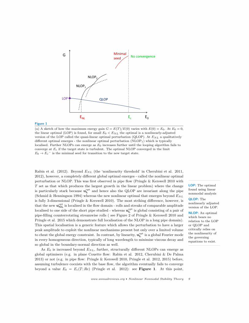
Figure 1

(a) A sketch of how the maximum energy gain G = E(T )/E(0) varies with E(0) = E0. At E0 = 0,

the linear optimal (LOP) is found, for small E0 < ENL the optimal is a nonlinearly-adjustedversion of the LOP called the quasi-linear optimal perturbation (QLOP). At ENL a qualitatively

different optimal emerges - the nonlinear optimal perturbation (NLOP1) which is typically

localised. Further NLOPs can emerge as E0 increases further until the looping algorithm fails toconverge at Ec if the target state is turbulent. The optimal NLOP converged in the limit

E0 → Ec− is the minimal seed for transition to the new target state.

Rabin et al. (2012). Beyond ENL (the ‘nonlinearity threshold’ in Cherubini et al. 2011,

2012), however, a completely different global optimal emerges - called the nonlinear optimal

perturbation or NLOP. This was first observed in pipe flow (Pringle & Kerswell 2010 with

T set as that which produces the largest growth in the linear problem) where the change

is particularly stark because uoptL and hence also the QLOP are invariant along the pipe

(Schmid & Henningson 1994) whereas the new nonlinear optimal that emerges beyond ENLis fully 3-dimensional (Pringle & Kerswell 2010). The most striking difference, however, is

that the new uoptNL is localised in the flow domain - rolls and streaks of comparable amplitude

localised to one side of the short pipe studied - whereas uoptL is global consisting of a pair of

pipe-filling counterrotating streamwise rolls ( see Figure 2 of Pringle & Kerswell 2010 and

Pringle et al. 2015 which demonstrate full localisation of the NLOP in a long pipe domain).

This spatial localisation is a generic feature which allows the perturbation to have a larger

peak amplitude to exploit the nonlinear mechanisms present but only over a limited volume

to cheat the global energy constraint. In contrast, by linearity, uoptL is a global Fourier mode

in every homogeneous direction, typically of long wavelength to minimise viscous decay and

so global in the boundary-normal direction as well.

LOP: The optimal

found using linearnonmodal analysis

QLOP: The

nonlinearly adjustedversion of the LOP.

NLOP: An optimal

which bears norelation to the LOP

or QLOP and

critically relies onthe nonlinearity of

the governingequations to exist.

As E0 is increased beyond ENL, further, structurally different NLOPs can emerge as

global optimisers (e.g. in plane Couette flow: Rabin et al. 2012, Cherubini & De Palma

2013) or not (e.g. in pipe flow: Pringle & Kerswell 2010, Pringle et al. 2012, 2015) before,

assuming turbulence coexists with the base flow, the algorithm eventually fails to converge

beyond a value E0 = Ec(T ;Re) (Pringle et al. 2012): see Figure 1. At this point,


the looping scheme has stumbled across an initial condition in the basin of attraction of

the turbulence which can reach the turbulent state by the target time. As a result, the

looping procedure becomes ill-conditioned due to the extreme sensitivity of the final state

energy to changes in the initial condition (Pringle et al. 2012). Reducing T allows NLOPs

to be converged at higher initial energies (Cherubini et al 2010, 2011, Cherubini & De

Palma 2013, Farano et al. 2015) whereas increasing T reduces Ec(T ;Re). This implies

the existence of a minimal finite (since the base flow is linearly stable) value Ec(∞;Re)

which represents the infimum on the disturbance energy which can trigger transition or,

equivalently, equals the minimum energy of any state on the laminar-turbulent boundary

or edge. States arbitrarily close to this minimal energy state - called the ‘minimal seed’

(Pringle et al. 2012) - and ‘above’ the edge (so outside the basin of attraction of the laminar

state) trigger turbulence. The closer they are to the minimal seed, the longer they take

to reach the turbulent state. Finding the form of the minimal seed is therefore central to

understanding transition in threshold conditions, that is, where transition is just triggered.

The evolution of the minimal seed itself is within the laminar-turbulent boundary or edge,

which is an invariant manifold, and is ultimately attracted to a relative attractor embedded

with it. This can be unique and simple (e.g. the equilibrium in Schneider et al. 2008) but

more generally is non-unique (§3.6 of Duguet et al. 2008) and chaotic (e.g. Schneider et

al. 2007, Mellibovsky et al. 2009). Either way, the minimal seed itself does not lead to

turbulence but there are states arbitrarily close to it which do. Identifying it is the first

application of the basic optimization approach just discussed.

4. Nonlinear Nonmodal Stability Analysis

Edge: The edge is a

hypersurface in

phase space whichseparates flow states

which evolve in

qualitativelydifferent ways.

4.1. Switching Basins of Attraction: Minimal Seeds for Transition

The approach to calculating the minimal seed assumes that as the disturbance energy

hypersurface expands (i.e. E0 increases), it first touches the laminar-turbulent boundary

or edge at precisely the energy E0 = Ec(T ;Re) (e.g. see the simple 2 ODE model of §2.1

in Kerswell et al. 2014). The common state on the two manifolds is then the minimal seed

as it has the lowest energy state on the edge. For E0 > Ec, so that now the edge punctures

the energy hypersurface, there exist initial conditions for the optimization procedure which

are in the basin of attraction of the turbulent state (or more generally are ‘above’ the edge

if the turbulence is instead a chaotic saddle). These can then achieve values of the objective

functional larger than any possible in the laminar basin of attraction (by design) and so

the optimization will track these. If the subsequent evolutions reach the turbulent state,

the looping algorithm will then fail to converge due to extreme sensitivity to the initial

conditions unless the objective functional has been specifically designed to average over the

final turbulent state in some way (Monokrousos et al. 2011). The procedure is then to

slowly increase E0 from a value where the algorithm converges until it no longer does due

to the existence of turbulent end states created by the looping iterates. The optimal of

the last successful convergence at E0 . Ec(T ;Re) is an approximation to the minimal seed

providing T is large enough (Pringle et al. 2012). A complementary approach is to start

with E0 & Ec where ‘turbulent seeds’ - initial conditions which lead to turbulence by T -

can be identified and then gradually reducing E0 (initiating with the previously identified

turbulent seeds at slightly higher E0) until no turbulent seeds can be found (Monokrousos

10 R. R. Kerswell

et al. 2011, Rabin et al. 2012, 2014). This latter approach can be quite efficient if the

starting E0 is sufficiently close to Ec as then the set of turbulent seeds will shrink down

smoothly to the minimal seed as E0 → Ec+, although there is always the danger of settling

on a local rather than global energy minimum of the edge.

Pringle et al. (2012) argue for why energy growth after time T might be the most

natural objective functional for this procedure, but actually any objective functional which

takes on heightened values in the basin of attraction of the turbulent state will do (e.g. total

dissipation over the trajectory - Monokrousos et al. 2011, Duguet et al 2013 and Eaves &

Caulfield 2015). The key point is that the optimization procedure should seek out any

initial condition on the energy hypersurface which is in the turbulent basin of attraction

if such states maximise the objective functional. Rabin et al. (2012) confirmed that the

same minimal seed emerged in plane Couette flow by using energy growth after time T as

when the total dissipation was used (Monokrousos et al. 2011). Practically, T has to be

chosen large enough to find the (globally) minimal seed and Ec(T ;Re) rather than just local

minima. However, evidence gathered so far using a variety of different T indicates that this

is not such a problem. For example, the NLOP first found in Pringle & Kerswell (2010) (see

their Figure 2) using a pipe only π/2 diameters long at Re = 1750 and T = 21D/U (where

D is the pipe diameter and U is the mean flow along the pipe) is recognisably the same

structure (albeit with no streamwise localisation and an extra symmetry: see Figure 8 of

Pringle et al. 2015) as that found at Re = 2400 in a pipe 5D long using T = 75D/U (see §5of Pringle et al. 2012) and in a pipe 50D long using T = 29.35D/U . In fact, the latter study

was able to reduce T down to ≈ 16D/U before finding any significant structural change in

the NLOP. There is also further indirect evidence for this robustness to the choice T in that

similar optimals are reported across a variety of flows: in plane Couette flow (Cherubini &

De Palma 2013, 2014a); the Blasius boundary layer (Cherubini et al. 2010, 2011, 2012);

the asymptotic suction boundary layer (Cherubini et al. 2015) and plane Poiseuille flow

(Farano et al. 2015, 2016). If T is too small, transients can obscure the situation (Rabin

et al. 2012) or new optimals become preferred (Pringle et al. 2015, Farano 2015). Another

potential problem is studying a flow where the turbulent state is not separated from the

laminar-turbulent boundary or edge as far as the objective functional is concerned. This is

a well-known issue with the technique of edge-tracking (Schneider & Eckhardt 2009) and

experience gained there indicates that provided the flow is not too tightly constrained (e.g.

the computational box is not too small) or too close to the first appearance of the turbulent

state (Re too low), the required separation exists.

4.1.1. Evolution. Once the minimal seed has been found, the evolution of a nearby turbulent

seed can be studied to uncover the optimal way (initiated by a disturbance of least energy)

to trigger transition. The fairly robust picture which emerges is that the minimal seed

is always spatially localised in all directions to allow much larger velocity amplitudes to

be accommodated than would be possible globally given the initial amplitude constraint

(for example see Figure 2). The minimal seed is also characterised by an initial flow

pattern which opposes the underlying mean shear so as to immediately benefit from the

Orr mechanism (Orr 1907). In this, the mean shear rotates the disturbance field around to

align with the mean flow direction creating some initial disturbance energy growth over a

fast time scale. Concurrently, the minimal seed also delocalises or ‘smears out’ due to the

mean shear before an ‘oblique wave phase’ of energy growth occurs over intermediate time

scales. This passes its energy into streamwise rolls which initiate a third growth process


Figure 2

The evolution of an initial condition close to but ‘below’ the minimal seed in a pipe 25D

(diameters) long with t = 0, 0.25, 0.5, 1, 2.5, 5, 10, 20 and Topt = 29.35D/U (going downwards: flowis from left to right) where U is the bulk speed along the pipe and Re := UD/ν = 2400 (see

figures 1 and 3 from Pringle et al. (2015) for alternative representations of the evolution) The

initially localised disturbance grows locally in amplitude and spatial extent evolving into analmost axially-invariant streak structure.

known as ‘lift up’ which operates over a comparatively slow (viscous) time scale (Pringle et

al. 2012, Duguet et al. 2013) to produce a predominately 2-dimensional streak field (e.g.

see the last 2 snapshots in Figure 2). For an initial condition just below the edge, this

streak field is linearly stable and the flow will ultimately decay. For an initial condition on

the edge, the streak field will then evolve into the (attracting) edge state whereas for an

initial condition just above the edge, the streak field is unstable, starts to bend and breaks

down to small scales signalling the turbulence state (e.g. Figure 12 of Pringle et al. 2012

and Duguet et al. 2013).

What is intriguing and also reassuring about this evolution is the fact that the finite-

amplitudeness of the minimal seed is able to symbiotically couple together - via the nonlin-

earity of the Navier-Stokes equations - three well-known linear growth mechanisms which

are staggered in time scale but uncoupled in the linearised Navier-Stokes equations. The

Orr mechanism is essentially a 2D spanwise-invariant process, while the oblique wave growth

is inherently 3D and the lift-up mechanism is optimised by 2D streamwise-invariant flows.

The minimal seed is able to take advantage of all 3 processes in turn by ensuring that the

energy growth of the preceding process is available to seed the next: see Appendix B of

Kerswell et al. (2014) for a simple example of this. The fact that retaining the nonlinearity

can then link these processes up is reassuring that the truly optimal (global) minimal seed

has been revealed by this procedure.

12 R. R. Kerswell

Essentially the same picture emerges from the Blasius boundary layer calculations of

Cherubini et al. (2011, 2012) although they work with short T and analyse a NLOP

computed some way ‘over’ the laminar-turbulent boundary rather than the minimal seed.

Although this NLOP seems to have the same localised structure - vortices inclined to the

streamwise direction positioned on the flanks of a region of intense streamwise velocity,

the various dynamical processes are not so well separated in time to the extent that the

formation of streaks and their subsequent instability are obscured by other instabilities.

Interestingly, they identify coherent structures reminiscent from DNS such as Λ vortices

and hairpin vortices in the evolution (e.g. see Figure 22 of Cherubini et al. 2011). Hairpin

vortices are also found to be generated by optimals computed in plane Poiseuille flow using

a very short T on the timescale of the Orr mechanism (Farano et al. 2015).

Once the minimal seed has been identified, its critical energy Ec can then be tracked as

a function of Re. This has been attempted in plane Couette flow at least up to Re = 3000

which suggests a scaling law Ec = O(Re−2.7) for the transition threshold (Duguet et al.

2013). This is significantly smaller than previous estimates of Ec = O(Re−2) (Duguet

et al. 2010) with the new feature being the spanwise localisation of the flow before streak

breakdown. A similar investigation has been carried out in the asymptotic suction boundary

layer for Re up to 5000 where a scaling of Ec = 0.38Re−2 is found (Cherubini et al. 2015).

This comfortably undercuts earlier estimates using initial conditions based upon: a) random

3-dimensional noise; b) streamwise vortices; c) oblique waves (Levin et al. 2005) and d)

two pairs of localised counterrotating vortices (Levin & Henningson 2007): see Figure 9 of

Cherubini et al. (2015) for a comparison.

4.2. Exploring Other Transition Scenarios

Beyond identifying the minimal seed and its subsequent evolution, other forms of transition

generated by larger disturbances can be uncovered using the optimization approach. In a

noisy environment, for example, where disturbance levels are much larger than the energy

level of the minimal seed, determining optimal routes to turbulence after a (short) time

horizon is of more natural concern. This, of course, is just the problem of computing Ec(T )

where T is finite and, as stressed above, may yield an approximation to the minimal seed

or a completely different optimal disturbance which starts off near a different part of the

edge, or is substantially removed from it if T is small enough. A good example of the latter

scenario is given by Cherubini & De Palma (2013) who found a bursting form of transition

in plane Couette flow by computing small T energy growth optimals at large E0 > ENL:

see Figure 3 and compare the top plots in their Figure 17. In this bursting transition, the

flow trajectory leaves the vicinity of the edge along a different unstable manifold than that

originating from the edge state, and so follows a different evolution than that of turbulent

seeds close to the minimal seed. This new manifold, which emerges from some other state

on the edge, plausibly forms a heteroclinic connection to a high energy state buried in the

basin of attraction of the turbulent state but not in the attractor itself: see Figure 4. A

similar phenomenon has been seen in stratified plane Couette flow where an initial burst

in energy is a precursor to the turbulent state and persists even when the turbulent state

is eventually suppressed by strong stable stratification (Olvera & Kerswell 2017). Farano

et al. (2017) have also looked for bursting events using a turbulent mean as the reference

state in channel flow. By tuning T to be the eddy turnover time at an ‘inner’ (in viscous

wall units y+ = 19) and ‘outer’ part (the centreline of the channel) of the flow, they find


X

2

4

6

8

10

12

Y

-1

0

1

Z

0

2

4

6

X

2

4

6

8

10

12

Y

-1

0

1

Z

0

2

4

6

Figure 3

Optimals for plane Couette flow (boundary at Y = ±1 moving in the ±X direction) at Re=400

obtained by nonlinear optimization with (E0, T ) = (0.05, 50) (left) and (0.0027, 300) (right) whichapproximates the minimal seed. Blue/yellow isosurfaces indicate negative/positive streamwise

velocity perturbation (contours ±0.06 left and ±0.013 right) whereas black/light gray ones

represent negative/positive spanwise velocity perturbation (±0.055 left and w = ±0.02 right).Data courtesy of Cherubini & De Palma (2013).

different bursting optimals which resemble observed large energy events.

Probing the early stages of transition has also been attempted by confining attention to

the initial approach to the edge state along its stable manifold. Here an objective functional

has been developed which balances minimising the initial energy of the perturbation with

the closeness with which it gets to the edge state over a range of T in plane Couette

flow (Cherubini & De Palma 2014b, 2015). The calculated optimal is found to become

successively less structured as T increases until the minimal seed emerges at large times:

Figure 5 of Cherubini & De Palma (2015) shows how the energy minimum converges to Ecfor large T .

In experiments where only specific forms of disturbance can be generated to initiate

transition - for example, injecting or removing fluid through small holes in the bound-

ary of pipe flow (Hof et al. 2003, Peixinho & Mullin 2007), the problem of interest

is typically to select the most dangerous such disturbance to trigger turbulence and

hence estimate Ec. In this case, the optimization procedure must be adapted to work

only over the reduced set of competitor initial conditions. This is easily accomplished

by projecting the variational derivative δL/δu(x, 0) down onto the subset of allowed

disturbances until a revised minimal seed emerges. This has not been done yet but

all the ingredients including the successful design of an artificial body forcing to theo-

retically model the inflow and ouflow jets (Mellibovsky & Meseguer 2009) are now available.

4.3. Detecting Nearby Saddles

A very similar optimization procedure can be used to explore the neighbourhood in phase

space of a (reference) flow state for nearby unstable states as that discussed above for

identifying minimal seeds. Providing the objective functional is chosen to be maximised

14 R. R. Kerswell

Turbulence

ES S1

S2

O

Edge

Figure 4

A sketch of phase space to illustrate how a different bursting transition scenario (initiated by a

disturbance of larger amplitude than the minimal seed) can occur than that which is mediated bythe edge state (ES). The reference state is the origin O of the coordinate system. S1 is a saddle

point on the edge (blue surface) and it is its unstable manifold perpendicular to the edge which

causes the bursting phenomenon leading the trajectory possibly up to another saddle S2 as shownbefore it ultimately gets attracted by the the turbulent attractor living at lower energy (energy is

depicted here as distance from O).

away from the reference state, the optimization procedure will select disturbances from the

energy hypersphere which lie nearest to or on the stable manifold of a nearby solution in

phase space, if T is large enough, as this is the best way to avoid converging back into the

reference state. The difference now, however, is since the nearby solution is unstable, T

cannot be too large otherwise even these disturbances will have decayed away (realistically

it is improbable to stay on the stable manifold to converge in to the unstable state). Once

such an optimal disturbance has been found, its temporal evolution will show evidence of

a transient approach to the new solution such as a plateauing of the objective functional

value in time if the new state is steady. A sufficiently close visit can yield a flow state

convergeable using a now-standard Newton-GMRES algorithm into the neighbouring state.

This has recently been demonstrated in wide-box plane Couette flow at low Re where

a multiplicity of states are known to co-exist (Olvera & Kerswell 2017). In particular, the

spanwise-localised ‘snake’ solution of Schneider et al. (2010) coexists with repeated copies

of the original global solution found by Nagata (1990) in a narrow domain. Not surprisingly,

the stable manifold of the ‘snake’ solution passes closer to the basic shear state (in energy

norm) than that of Nagata’s solution. However, the latter offers the possibility of greater

energy growth as it is global and hence is preferred if reachable from the hypersurface of

initial conditions. As a result, there is an energy threshold for which the optimal transiently

approaches the snake solution - see Figure 5 - and a yet higher threshold beyond which


0 50 100 150 2000

0.2

0.4

0.6

0.8

1

1.2

Res

idua

l, G

/100

m0 20 40 60 80 100 120 140 160 180 200 2200

0.005

0.01

0.015

0.02

0.025

0.03

Time

E

0 π 2π 3π 4π 5π 6π 7π 8π 9π 10π 11π 12π 13π 14π 15π 16π−1

−0.5

0

0.5

1

Z

Y


−0.5

0

0.5

1

Z

Y


−0.5

0

0.5

1

Z

Y


−0.5

0

0.5

1

Z

Y


−0.5

0

0.5

1

Z

Y


−0.5

0

0.5

1

Z

Y


−0.5

0

0.5

1

Z

Y


−0.5

0

0.5

1

Z

Y


−0.5

0

0.5

1

Z

Y


−0.5

0

0.5

1

Z

Y

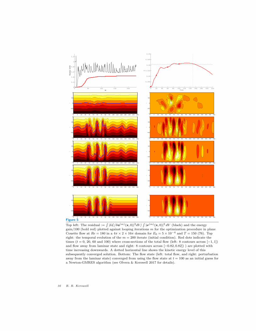
Figure 5

Top left: The residual :=∫|δL/δu(m)(x, 0)|2dV/

∫|ν(m)(x, 0)|2 dV (black) and the energy

gain/100 (bold red) plotted against looping iterations m for the optimization procedure in plane

Couette flow at Re = 180 in a 4π × 2× 16π domain for E0 = 5× 10−4 and T = 150 (76). Topright: the temporal evolution of the m = 200 iterate (initial condition). Red dots indicate thetimes (t = 0, 20, 60 and 100) where cross-sections of the total flow (left: 8 contours across [−1, 1])and flow away from laminar state and right: 8 contours across [−0.82, 0.82]) ) are plotted with

time increasing downwards. A dotted horizontal line shows the kinetic energy level of thissubsequently converged solution. Bottom: The flow state (left: total flow, and right: perturbation

away from the laminar state) converged from using the flow state at t = 100 as an initial guess fora Newton-GMRES algorithm (see Olvera & Kerswell 2017 for details).

16 R. R. Kerswell

Nagata’s solution is approached (see §6.3 in Rabin 2013). Figure 5 shows the plateauing

in the objective functional over t ∈ [80, 160] and snapshots of the evolving flow state. The

last flow state shown at t = 100 converges using a Newton-GMRES algorithm to the exact

solution shown at the bottom of the figure (Olvera & Kerswell 2017). The procedure works

just as well to isolate Nagata’s solution.

This approach can be used to look for new solutions in regions of parameter space where

little is known. For example, the simple shear state is provably unique in plane Couette

flow for Re < 20.7 and provably non-unique for Re ≥ 127.7 where Nagata’s solution exists.

However, a preliminary search has so far found nothing at Re = 100 (Olvera & Kerswell

2017) suggesting that the uniqueness of the simple shear state extends up to here and

probably all the way to 127.7.

4.4. Stability of Temporally- and Spatially-Evolving flows

4.4.1. Spatially-Evolving Flows. The linear (modal) stability analysis of spatially-evolving

flows can either be attempted locally, by assuming the base flow is slowly varying relative

to the disturbance being considered, or globally, by considering a large domain and looking

for growing global disturbances (e.g. see Chomaz (2005)). With increasing computational

power, the latter has naturally become more prevalent although it is still computationally

expensive. Nonmodal analysis (linear or nonlinear) can be carried out in either but the time

horizon over which energy growth is sought is then restricted by the timescale over which

the base flow is seen to vary by the disturbance or the transit time of the flow through the

truncated domain. For example, in the Blasius boundary layer calculations of Cherubini et

al. (2010), the boundary region studied is x ∈ [200, 400], where the leading edge is at x = 0

and the evolving disturbance is forced to vanish at either end of this domain. The nonlinear

optimals which emerge are necessarily positioned near the upstream domain boundary and

T is taken small enough so that disturbance doesn’t interact with downstream boundary.

Providing this global approach is taken, nonmodal analysis is straightforward to formulate

since the starting position of the optimal disturbance emerges as part of the optimization

procedure once the exact (spatial) domain of interest has been chosen. For a time-evolving

base state situation, however, knowing when to start the optimization procedure - i.e.

introduce the disturbance - is a nontrivial consideration and it is to this situation we now

turn.

4.4.2. Time-Periodic States. In the periodic case, the usual choices for a modal analysis

are again local in time - a ‘quasi-static’ analysis in which the base flow is assumed frozen

in time - and a global-in-time formal Floquet analysis. The latter can identify modal

energy growth across one period only which repeats to give asymptotically sustained growth.

However, there may be strong nonmodal energy amplification of infinitesimal disturbances

within a subinterval of a period which happens to decay by the end of the period and/or

transient energy growth over multiple periods, both of which can be identified by a linear

nonmodal analysis (see §3.3 of Schmid (2007)). Determining at what finite amplitude of

disturbance either of these transient effects may trigger transition requires a nonlinear

nonmodal stability analysis. Two thresholds can be pursued. The first is for a turbulent

state to be triggered within a period (small T ) but which relaminarises by the end of it

and the second, larger threshold is for sustained turbulence which persists once triggered

over subsequent periods (large T ). In the latter, the objective functional may need to be


some sort of a time average of the energy or dissipation rate over the latter part of the

time period to keep the variational derivatives relatively smooth when transient turbulence

is triggered, but sustained turbulence is not yet been reached (e.g. see Monokrousos et al.

2011).

In either situation, the time origin for the optimization procedure must either be a

priori chosen (and then optimised over as done in Rabin et al. 2014) or calculated as part

of the optimization procedure. In the latter situation, the Lagrangian (expression (4) ) can

be rewritten as

L = E(T + T0) + λ {E(T0)− E0} +

∫ T+T0

T0

〈{ · · · }〉dt.

where E(t) := 〈 12u(x, t)2〉 is the kinetic energy, T0 is now a variable time origin relative to

the base state and, as before, T is the time horizon. The Euler-Lagrange equation for T0

(keeping T fixed) is then simply

δL∂T0

=∂E

∂t

∣∣∣∣T+T0

+ λ∂E

∂t

∣∣∣∣T0

(19)

(assuming that the Navier-Stokes equation and incompressibility are imposed at T0 and

T0+T ) which can be straightforwardly incorporated in the looping algorithm. Here δL/∂T0

is evaluated at the end of a loop (when both u(x, T0) and u(x, T0 + T ) are available) and

then used to move T0 in the direction of increasing L for the next loop (u(x, T0) is then

used to initiate the next loop at this new time). Rabin et al. (2012) experimented with

optimising T (keeping T0 = 0) in plane Couette flow when looking for the minimal seed but

found that T could become small caused by short term transients which complicated the

results.

An outstanding example of where this analysis could be useful is Stokes’ second problem

of an oscillating plate bounding a semi-infinite (y ≥ 0) fluid-filled domain. There the base

flow is

U(y, t) = cos(2πt−√π y)e−

√π y (20)

where the period of oscillation T and diffusive length scale√νT are used as units of time

and length respectively (ν being the kinematic viscosity). Defining a Reynolds number as

Re := U√T/ν where U is the maximum speed of the oscillating plate (after Biau 2016), a

quasi-static linear analysis gives an estimate of the critical Re as 152 for linear instability

whereas a (proper) Floquet analysis gives a figure of 2511 (see Ozdemir et al. 2014 for

references). The actual transitional Re, however, is firmly in the middle of these theoretical

estimates at about 900, indicating a finite-amplitude instability. A recent (linear) nonmodal

analysis reveals that infinitesimal disturbances can experience huge energy growth - e.g. a

growth factor of 3.8 × 106 at Re = 1000 (see Table 1 of Biau 2016) - over a sub-interval

of an oscillation through the Orr mechanism, suggesting that the (finite) energy thresholds

for partial or sustained turbulence may be very small. This would imply that the finite

amplitude instability can be triggered very easily in both experiments by ambient noise

and numerical simulations by the supposedly small initial conditions used to initiate runs

(Ozdemir et al. 2014). The linear nonmodal analysis also indicates that only the Orr

mechanism is important and so the optimal starting time found there may be good for the

nonlinear nonmodal analysis too: see Table 1 of Biau (2016).

18 R. R. Kerswell

−1 −0.5 0 0.5 1−1

−0.8

−0.6

−0.4

−0.2

0

0.2

0.4

0.6

0.8

1

U

y

00.20.50.831.2

∞

0 0.2 0.4 0.6 0.8 1 1.2

1

1.5

2

2.5

3

3.5

4x 10

4

Re c

η := 4 ( t / Re )1/2

85920.83

0.918

5.311

3.547

2.128

1.3980.496

0.232

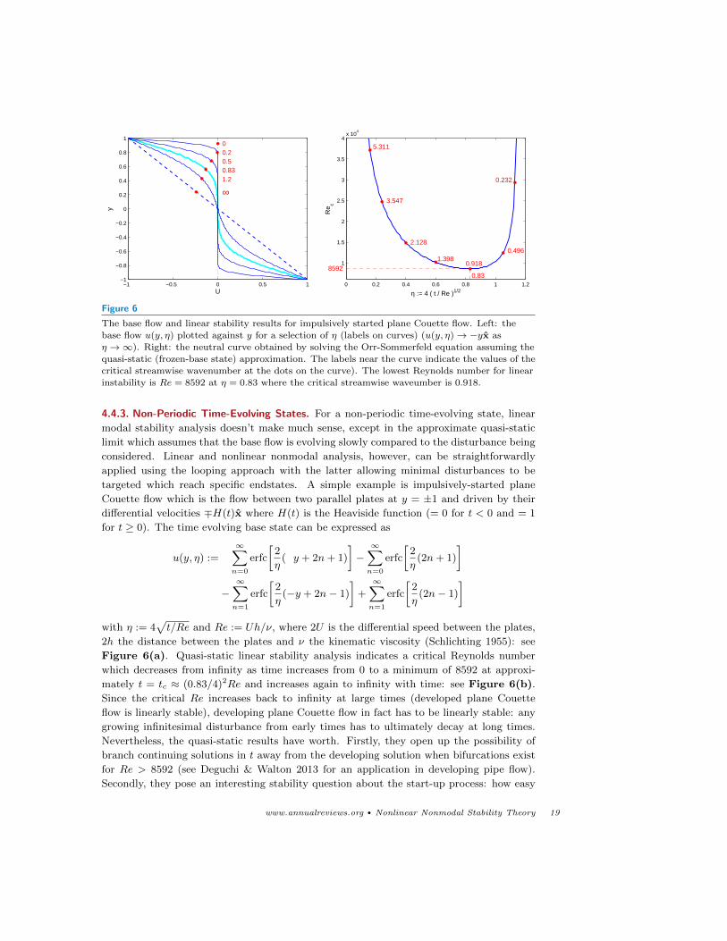
Figure 6

The base flow and linear stability results for impulsively started plane Couette flow. Left: the

base flow u(y, η) plotted against y for a selection of η (labels on curves) (u(y, η)→ −yx asη →∞). Right: the neutral curve obtained by solving the Orr-Sommerfeld equation assuming the

quasi-static (frozen-base state) approximation. The labels near the curve indicate the values of the

critical streamwise wavenumber at the dots on the curve). The lowest Reynolds number for linearinstability is Re = 8592 at η = 0.83 where the critical streamwise waveumber is 0.918.

4.4.3. Non-Periodic Time-Evolving States. For a non-periodic time-evolving state, linear

modal stability analysis doesn’t make much sense, except in the approximate quasi-static

limit which assumes that the base flow is evolving slowly compared to the disturbance being

considered. Linear and nonlinear nonmodal analysis, however, can be straightforwardly

applied using the looping approach with the latter allowing minimal disturbances to be

targeted which reach specific endstates. A simple example is impulsively-started plane

Couette flow which is the flow between two parallel plates at y = ±1 and driven by their

differential velocities ∓H(t)x where H(t) is the Heaviside function (= 0 for t < 0 and = 1

for t ≥ 0). The time evolving base state can be expressed as

u(y, η) :=

∞∑n=0

erfc

[2

η( y + 2n+ 1)

]−∞∑n=0

erfc

[2

η(2n+ 1)

]

−∞∑n=1

erfc

[2

η(−y + 2n− 1)

]+

∞∑n=1

erfc

[2

η(2n− 1)

]with η := 4

√t/Re and Re := Uh/ν, where 2U is the differential speed between the plates,

2h the distance between the plates and ν the kinematic viscosity (Schlichting 1955): see

Figure 6(a). Quasi-static linear stability analysis indicates a critical Reynolds number

which decreases from infinity as time increases from 0 to a minimum of 8592 at approxi-

mately t = tc ≈ (0.83/4)2Re and increases again to infinity with time: see Figure 6(b).

Since the critical Re increases back to infinity at large times (developed plane Couette

flow is linearly stable), developing plane Couette flow in fact has to be linearly stable: any

growing infinitesimal disturbance from early times has to ultimately decay at long times.

Nevertheless, the quasi-static results have worth. Firstly, they open up the possibility of

branch continuing solutions in t away from the developing solution when bifurcations exist

for Re > 8592 (see Deguchi & Walton 2013 for an application in developing pipe flow).

Secondly, they pose an interesting stability question about the start-up process: how easy


is it to influence the endstate reached via a finite-amplitude disturbance after a certain time

when there are multiple attractors? This is a generalised minimal seed question since the

time of disruption as well as the optimal disturbance must be sought to minimally disturb

the evolving simple shear state to an alternate attractor (e.g. turbulence at high Re). In

the first instance, if only one alternative attractor is present (the generic situation in plane

Couette flow at high enough Re), using the final energy of the disturbance away from the

simple shear state as the objective functional should work provided a ‘long’ time horizon

T is chosen. The time-evolving mixing layer (e.g. Arratia et al. 2013) is another good

example of where this approach may be used profitably.

5. Other Applications

5.1. Weather Forecasting and Sensitivity

In weather forecasting, an important issue is the short time behaviour of a predictive model

initiated with imperfect initial data (the state of the atmosphere is never known everywhere

at once). Understanding the sensitivity of the model to errors in the initial data is then

paramount for assessing the subsequent errors in forecasts. Ensemble forecasts (Palmer et

al. 1993, Buizza & Palmer 1995) attempt to estimate the likely uncertainty in the forecast

by considering an ensemble of runs initiated with data polluted by the most ‘dangerous’

errors. These most dangerous errors are taken to be the singular value vectors or nonmodal

(linear) optimals calculated from the linear operator based upon the unpolluted prediction

and are then assigned some finite amplitude. There have been attempts to incorporate

nonlinearity into this by an iterative approach (Oortwijn and Barkmeijer 1995, Barkmeijer

1996) as well as a fully nonlinear approach (Mu 2000, Mu et al. 2003, Mu & Zhang 2006,

Mu & Jiang 2008a,b, Mu et al. 2010, Duan & Zhou 2013, Jiang et al. 2013, Ziqing et al.

2013, Dijkstra & Viebahn 2015). Of key concern is that given the amplitude of perturbation

assumed, fully nonlinear optimals may indicate a completely different response of the system

compared to the linear optimals precisely because the perturbation is finite amplitude. This

will then have implications for the probability distribution of what the true forecast is some

given time later.

Mu and coworkers have also computed nonlinear optimals - or ‘conditional nonlinear

optimal perturbation’ (CNOP) in their words - to study the sensitivity of other weather

and climate events such as El Nino events (Yu et al. 2009, Duan et al. 2013, Mu et

al. 2013), ‘blocking’ onsets (Mu & Jiang 2008b, 2011 and Jiang & Wang 2010) and the

Kuroshio large meander (Wang et al. 2012, 2013), and to probe nonlinear stability of

simple oceanographic models (Mu et al. 2004, Mu & Zhang 2006). In their first study, Mu

et al. (2004) considered a very simple (2-dimensional ODE) box model of the thermohaline

circulation but subsequent work (Mu & Zhang 2006) scaled this effort up to a 2-dimensional

quasigeostrophic model with 512 grid points. van Scheltinga & Dijkstra’s (2008) model

of a double-gyre ocean circulation, which uses 4800 degrees of freedom, represents the

most ambitious application so far in this context. Given that the Navier-Stokes equation

discretised using millions of degrees of freedom has now been handled successfully in the

transition to turbulence context, there is clearly an opportunity to push this work further.

20 R. R. Kerswell

5.2. Thermoacoustics

The optimization approach to identify the critical disturbance of one linearly-stable state so

that another state is reached has also been used in thermoacoustics. Juniper (2011a,b) has

studied the horizontal Rijke tube, which is modelled by a couple of 1-space 1-time PDEs,

using this approach. Here the laminar state is a fixed point, the edge state is an unstable

periodic orbit and the ‘turbulent’ state is a stable periodic orbit (respectively the ‘lower’

and ‘upper’ branches which emerge from a saddle node bifurcation). The Rijke tube system

is sufficiently simple that an exhaustive study of optimal energy growth can be carried

out over both amplitude and time horizon T to confirm the predictions of the nonlinear

optimization procedure (Juniper 2011b).

5.3. Magnetic Field Generation and Mixing in Stratified flows

Two very different applications have been attempted following the success of the nonlinear

looping approach in the transition problem. In 2012, Willis considered the kinematic dy-

namo problem in magnetohydrodynamics, which asks the question of whether a magnetic

field B can grow on a velocity field u in an electrically conducting fluid. This is usually

formulated by assuming a specific form for the velocity field and then converting the in-

duction equation for the magnetic field into an eigenvalue problem. However, Willis (2012)

formulated a novel optimization problem to both identify the magnetic field and velocity

field which together give the largest magnetic field growth for a given magnetic Reynolds

number Rm. The only constraints on the velocity field are incompressibility, periodicity

(calculations are performed in a triply periodic box) and fixed energy dissipation rate (or,

equivalently, fixed power input) so that the Lagrangian is

L = 〈B2T 〉 − λ1(〈(∇× u)2〉 − 1)− λ2(〈B2

0〉 − 1)− 〈Π1∇ · u〉 − 〈Π2∇ ·B0〉

−∫ T

0

〈Γ ·[∂B

∂t−∇× (u×B)− 1

Rm∇2B

]〉dt (21)

where B0 is the initial magnetic field, BT the final magnetic field at t = T and λi, Πi and Γ

are Lagrange multipliers. In this formulation, the induction equation is now fully nonlinear

since both B and u are unknowns. This work has been extended to finite fluid-filled domains

which adds the extra complication of matching the magnetic field to surrounding (external)

conditions (Chen et al. 2015).

In 2-dimensional channel flow, Foures et al. (2014) have identified initial velocity fields

u(x, t) which lead to ‘maximal’ mixing of a passive scalar θ(x, t) depending on exactly how

this mixing is quantified. The scalar is initially arranged in two unmixed layers of different

concentrations meeting at the midplane of the channel and a number of different objective

functionals

L :=1

2(1− α)

∫ T

0

〈u(x, t)2〉 dt+1

2α〈|∇−βθ(x, T )|2〉 (22)

extremised using the nonlinear looping approach. Optimal initial velocity conditions which

maximise the time-averaged energy (α = 0), minimise the variance of the passive scalar

(α = 1, β = 0) or minimise the ‘mix-norm’ of the scalar (α = 1, β = 1) are each tested to

see how effective their subsequent evolution is in mixing up the scalar field.


5.4. Control

Once the nonlinear stability of a given flow has been quantified by identifying the critical

disturbance energy and structure, it becomes feasible to attempt to design a more (or less)

nonlinearly stable flow by changing some aspect of the system. Rabin et al. (2014) tried

just this in plane Couette flow by adding an extra spanwise oscillation (amplitude A and

frequency ω) of both boundaries to their relative motion so that the boundary motion at

y = ±1 is

u(x,±1, z, t) = ∓x +A sin(ωt)z (23)

(using the set-up of §4.4.3). This modified boundary motion leads to the revised basic flow

response uA(x, t;A,ω,Re) and the question is then: can A and ω be chosen such that uAis more nonlinearly stable (where ‘more stable’ means the energy of the critical disturbance

to reach the basin boundary, Ec, is increased)? As the reference state is time-periodic,

the nonlinear nonmodal analysis is more intensive as an extra search has to be conducted

over the exact time within a period when the disturbance is introduced. Despite this extra

overhead, Rabin et al. (2014) show that there is a sweet spot in the (A,ω) plane where the

flow uA can be made 41% more stable than the unoscillated basic flow at Re = 1000 (i.e.

Ec is 1.41 × the uncontrolled value). The implication is that if the ambient noise level is

between the unoscillated and oscillated values, there are power savings to be had since uAwill be stable to the noise while the unoscillated system should be turbulent and therefore

consume much more power. This is very much a proof-of-concept computation in that 1)

no robustness of the the sweet spot over Re was demonstrated and, more seriously, 2) the

optimization approach assumes the introduction of one disturbance only and its subsequent

evolution rather than a continual stream of disturbances. This latter assumption can be

lifted by opening up the optimization to multiple disturbances distributed over the time

interval [0, T ] but then the exact amplitude condition to constrain different disturbance

patterns is less clear (Lecoanet & Kerswell 2013). For example, the energy of two identical

disturbances occuring at different times is half the energy measure if the two disturbances

occur simultaneously. This is, however, an interesting direction for further work.

Other work stimulated by the recent success of nonlinear looping is that of Passaggia

and Ehrenstein (2013) who have looked at controlling the 2-dimensional boundary layer

dynamics over a bump by blowing and sucking using the full Navier-Stokes equation. This

has been extended to 3 dimensions by Cherubini et al. (2013) where the linear and non-

linear optimals have been used as initial conditions. This work remains a long way off real

applications because it relies on knowing the state of the system at each time and perform-

ing costly optimization calculations, which can’t be done in real time, so the use of fully

nonlinear methods in control are still impractical (e.g. Joslin et al. 1995, 1997, Gunzburger

2000, Bewley et al. 2001, Chevalier et al. 2002, Pralits et al. 2002, Kim & Bewley 2007).

6. Summary and Future Directions

This article has described a new optimization technique for analysing the nonlinear stability

of a reference state. This is ostensibly for a linearly stable state and then the fundamental

question is: what sort of disturbance will shift the system beyond the state’s basin of

attraction? However, it can also be useful for linearly unstable states if the timescale of the

linear instability is much longer than the time horizon of interest (e.g. in Blasius boundary

layer flow). Then ‘bypass’ processes acting on shorter timescales can be analysed as if the

22 R. R. Kerswell

reference state is stable. The core of the approach is to ‘nonlinearise’ nonmodal analysis

so that competing disturbances of a given fixed finite amplitude are considered to optimise

an objective functional, constrained by the fact that each disturbance evolves subject to

the full Navier-Stokes equation. The discussion has focussed on the final energy growth of

the disturbance mostly for simplicity and historical reasons, but in fact this is a sensible

default choice for most applications because the asymptotic limit of disturbance energy

clearly signals whether the disturbance started inside, on or outside the basin boundary of

the reference state.

As stated earlier, the idea to extend nonmodal analysis to treat finite amplitude distur-

bances is not particularly profound. Neither is the observation that the optimal value of

the objective functional will undergo a sudden change to larger values as the initial distur-

bance amplitude is increased beyond the point where some can explore parts of phase space

beyond the basin of attraction. Instead, what is noteworthy is the recent realisation that

the fully nonlinear non-convex optimization problem so formulated can actually be solved

using a direct-adjoint looping approach on large degree-of-freedom systems to give credible

results. Conceptually, this procedure provides a theoretical bridge between the two comple-

mentary perspectives of linear nonmodal analysis (which technically includes linear stability

analysis if T → ∞) and the (nonlinear) dynamical systems approach to fluid mechanics.

The strict inclusion of nonlinearity means the approach is necessarily computational and

has its uncertainties (e.g. identifying global over local optimals). However, the fact that

the nonlinear optimals which have emerged so far appear to be as a concatenation of linear

processes hints that a simpler semi-analytical framework could be available (e.g. see Pralits

et al. 2015 for some work in this direction).

This article has also tried to indicate how flexible this optimization approach is. Al-

though the focus has been on bistable systems, multistable situations can be handled pro-

viding the objective functional is designed to pick out the desired target state. A long-lived

transient state can also be targeted which is actually what was originally treated since the

turbulence in shear flows at low Reynolds number and in constrained computational do-

mains tends only to be a chaotic repellor (e.g. the short periodic pipe of Pringle & Kerswell

2010). Some preliminary work using nonlinear nonmodal analysis has also been described

to probe phase space for unstable solutions nearby to the reference state (Olvera & Kerswell

2017).

The technique as described here specifically considers only one finite-amplitude distur-

bance and then considers its evolution in the absence of any further disturbances. This is

sufficient to gauge the nonlinear stability of the reference state but, in practice, flows can

be exposed to multiple, if not a continuous stream, of disturbances and how these interact

to push the system to another attractor is more important. The optimization approach

can be straightforwardly extended to consider multiple disturbances distributed across an

interval and there is an interesting connection to be made with the continuously disturbed

or ‘noisy’ situation (Freidlin & Wentzell 1998, Waugh & Juniper 2011, Wang et al. 2015,

Lecoanet & Kerswell 2017).

A number of areas ripe for future development have also been discussed. Perhaps most

obvious is the treatment of time-periodic states. The procedure is more arduous in this

case - an extra optimization over the disturbance time is required - but still doable and

the easier linear calculation may suggest a shortcut through this. Some aperiodic flows like

an impulsively started flow or the diffusing mixing layer situation can also be treated in

the same way, where the optimal time to add the disturbance can be narrowed down by a


linear quasi-static analysis. However, it is presently unclear how to handle reference states

which are quasi-periodic or even chaotic and a more natural approach would be to consider

noise instead. Another area is ‘design’. The ability to quantify the nonlinear stability of

a state opens up the possibility of manipulating the system to produce a ‘better’ flow,

whether this be more or less stable. This idea has been briefly explored by actively (using

more power) modifying the motion of the boundaries in plane Couette flow but there are

interesting passive options (requiring no additional power) such as adjusting the shape of

the boundaries to be explored. The technique can also be used to help design experiments

where typically a limited suite of perturbations are available to the experimentalist. The

search for an optimal disturbance to trigger a desired effect (e.g. transition or a large

amplitude event) can then be simply restricted to those which are practical, avoiding a

trail-and-error approach.

In conclusion, nonlinear nonmodal analysis appears to be a valuable tool to probe

the dynamics around a given reference state. Coupled to a search over the amplitude of

the competing disturbances, a computational tool emerges to probe basin boundaries and,

if the ‘other’ state is turbulence, the transition problem. Challenges exist to lessen the

computational overhead and perhaps even to make part of the procedure semi-analytic, but

with ever-increasing computational power, it’s hard not to envisage this technique becoming

a standard theoretical tool in fluid mechanics.

SUMMARY POINTS

1. Nonlinear nonmodal analysis. It is now feasible to identify a disturbance of a

given initial (finite) amplitude to a reference state which maximises the energy

growth some time later using an iterative direct-adjoint looping procedure thereby

extending (linear) nonmodal analysis. This has recently been performed for flow

systems with millions of degrees of freedom, is easily extendable to treat other

objective functionals and can be used to investigate phase space beyond that which

immediately surrounds the reference state.

2. Nonlinear nonmodal stability analysis. Providing the objective functional to be

maximised is chosen so that it takes heightened values at the new attracting target

state, nonlinear nonmodal analysis can be coupled with a search over disturbance

amplitude to identify the critical disturbance which corresponds to the closest

point of approach of the basin boundary to the reference state. For the transition

problem, this critical disturbance is called the minimal seed for transition and is

arbitrarily close to initial conditions beyond the basin boundary which lead to

turbulence.

3. Bridging a gap. Nonlinear nonmodal stability analysis bridges the conceptual

gap between (linear) nonmodal stability theory which focusses on the behaviour

in the immediate neighbourhood of a reference state and the (fully nonlinear)

dynamical systems approach to fluid mechanics. By identifying the critical distur-

bance for a given amplitude measure, the nonlinear stability of a flow state can

now be quantified which can then be used to design a more stable or less stable state.

4. Flexibility. The general approach is one of optimization of a chosen objective func-

24 R. R. Kerswell

tional subject to constraints which include the full Navier-Stokes equations and

is therefore incredibly flexible. The nonlinear stability of time-evolving reference

states can be considered as can optimal starting conditions identified which lead to

desired flow episodes (e.g. large energy events such as ‘bursting’ or transition by a

certain time).

FUTURE ISSUES

1. Convergence. Implementations of nonlinear nonmodal analysis sometimes show

stalling convergence even though a reasonable optimal still appears to emerge.

Work is needed to understand this and to improve the update procedure for the

optimal in the direct-adjoint looping iterations. Currently there is no specific

tailoring of this procedure to the likely form of the optimal (e.g. the NLOP is

generically fully localised in space) or for what initial conditions can be generated

in the laboratory.

2. Multiple disturbances. This article discusses the implications of applying a single

disturbance to a flow system and then studying its subsequent evolution free

of any further disturbances. While useful for formally assessing the nonlinear

stability of the reference state, this is less relevant to a reference state continually

being exposed to disturbances. Multiple disturbances can be handled using the

optimization approach of this article and connecting this with the continuous noise

limit (large deviation theory and ‘instantons’) is an interesting future direction.

3. Applications. The most obvious new direction for applications is the treatment

of time-dependent reference states. Even the simplest scenario of a time-periodic

state leads to a more involved optimization procedure since the application

time for the disturbance ostensibly needs to be optimized over. Avoiding this

extra search by exploiting some physical insight as, for example, provided by the

(linear) nonmodal analysis over short times would represent a valuable step forward.

4. Design. The ability to quantify the nonlinear stability of a given flow state opens

up the possibility of then subsequently manipulating or designing a ‘better’ system

whether this means one with a more or less stable reference state. So far only one

proof-of-concept calculation has been done by introducing an extra motion of the

boundary so developing this idea further (e.g. to include boundary shape design)

is an exciting direction for future work.

DISCLOSURE STATEMENT

The author is not aware of any affiliations, memberships, funding, or financial holdings that

might be perceived as affecting the objectivity of this review.


ACKNOWLEDGEMENTS

I’d like to thank Stefania Cherubini, Jake Langham and Jacob Page for commenting on an

early version of the manuscript. Thanks also to Chris Pringle, Stefania Cherubini (again)

and Daniel Olvera for helping to produce Figures, 2, 3 and 5 respectively.

LITERATURE CITED

Arratia C, Caulfield CP, Chomaz J-M. 2013. Transient perturbation growth in time-dependent

mixing layers. J. Fluid Mech. 717:90–133

Andersson P, Berggren M, Henningson DS. 1999. Optimal disturbances and bypass transition in

boundary layers. Phys. Fluids 11:134–150

Barkmeijer J. 1996. Constructing fast-growing perturbations for the nonlinear regime. J. Atmos.

Sci. 53:2838–2851

Berggren M. 1998. Numerical solution of a flow-control problem: vorticity reduction by dynamic

boundary action. Siam J. Sci. Comput. 19:829–860

Bewley TR, Moin P, Temam R. 2001. DNS-based predictive control of turbulence: an optimal

benchmark for feedback algorithms. J. Fluid Mech. 447:179–225

Biau D. 2016. Transient growth of perturbations in Stokes oscillatory flows. J. Fluid Mech. 794:R4

Boberg L, Brosa U. 1988. Onset of turbulence in a pipe. Z. Naturforsch. 43a:697–726

Buizza R, Palmer TN. 1995. The singular-vector structure of the atmospheric global circulation. J.

Atmos. Sci. 52:1434–1456

Butler KM, Farrell BF. 1992. 3-Dimensional optimal perturbations in viscous shear-flow. Phys.

Fluids 4:1637–1650

Chen L, Herreman W, Jackson A. 2015. Optimal dynamo action by steady flows confined to a cube.

J. Fluid Mech. 783:23–45

Cherubini S, De Palma P, Robinet J-C, Bottaro A. 2010. Rapid path to transition via nonlinear

localised optimal perturbations in a boundary layer flow. Phys. Rev. E 82: 066302

Cherubini S, De Palma P, Robinet J-C, Bottaro A. 2011. The minimal seed of turbulent transition

in the boundary layer. J. Fluid Mech. 689:221–253

Cherubini S, De Palma P, Robinet J-C, Bottaro A. 2012. A purely nonlinear route to transition

approaching the edge of chaos in a boundary layer. Fluid Dynam. Res. 44:031404

Cherubini S, De Palma P. 2013. Nonlinear optimal perturbations in a Couette flow: bursting and

transition. J. Fluid Mech. 716:251–279

Cherubini S, Robinet J-C, De Palma P. 2013a. Nonlinear control of unsteady finite-amplitude per-

turbations in the Blasius boundary-layer flow. J. Fluid Mech. 737:440–465

Cherubini S, De Palma P. 2014a. Minimal perturbations approaching the edge of chaos in a Couette

flow. Fluid Dynam. Res. 46:041403

Cherubini S, De Palma P 2014b. Minimal-energy perturbations rapidly approaching the edge state

in Couette flow. J. Fluid Mech. 746:572–598.

Cherubini S, De Palma P, Robinet J-C. 2015. Nonlinear optimals in the asymptotic suction boundary

layer: transition thresholds and symmetry breaking. Phys. Fluids 27:034108.

Chevalier M, Hogberg M, Berggren M, Henningson DS. 2002. Linear and nonlinear optimal control

in spatial boundary layers. AIAA paper 2002–2755 3rd Theoretical Fluid Mechanics Meeting,

St Loius, Missouri

Chomaz J-M. 2005. Global instabilities in spatially developing flow: Non-normality and nonlinearity.

Ann. Rev. Fluid Mech. 37:357–392

Corbett P, Bottaro A. 2000. Optimal perturbations for boundary layers subject to streamwise

pressure gradient. Phys. Fluids 12:120–130

Deguchi K, Walton AC. 2013. A swirling spiral wave solution in pipe flow. J. Fluid Mech. 737:R2

Dijkstra H, Viebahn JP. 2015. Sensitivity and resilience of the climate system: a conditional non-

26 R. R. Kerswell

linear optimization approach. Commun. Nonlinear Sci. Numer. Simulat. 22:13–22

Duan W, Yu Y, Xu H, Zhao P. 2013. Behaviors of nonlinearities modulating the El Nino events

induced by optimal precursory disturbances. Clim. Dyn. 40:1399–1413

Duan W, Zhou F. 2013. Non-linear forcing singular vector of a two-dimensional quasi-geostrophic

model. Tellus 65:18452

Duguet Y, Willis AP, Kerswell RR. 2008. Transition in pipe flow: the saddle structure on the

boundary of turbulence. J. Fluid Mech. 613:255–274

Duguet Y, Brandt L, Larsson BRJ. 2010. Towards minimal perturbations in transitional plane

Couette flow. Phys. Rev. E 82:026316

Duguet Y, Monokrousos A, Brandt L, Henningson DS. 2013. Minimal transition thresholds in plane

Couette flow. Phys. Fluids 25:084103

Eaves TS, Caulfield CP. 2015. Disruption of SSP/VWI states by a stable stratification. J. Fluid

Mech. 784:548–564

Eckhardt B, Schneider T M, Hof B, Westerweel J. 2007. Turbulence transition in pipe flow. Ann.

Rev. Fluid Mech. 39:447–468

Farano M, Cherubini S, Robinet J-C, De Palma P. 2015. Hairpin-like optimal pertubations in plane

Poiseuille flow. J. Fluid Mech. 775:R2

Farano M, Cherubini S, Robinet J-C, De Palma P. 2016. Subcritical transition scenarios via lin-

ear and nonlinear localized optimal perturbations in plane Poiseuille flow. Fluid Dynam. Res.

46:061409

Farano M, Cherubini S, Robinet J-C, De Palma P. 2017 Optimal bursts in turbulenty channel flow.

J. Fluid Mech. 817:35–60

Farrell BF. 1988. Optimal excitation of perturbations in viscous shear flow. Phys. Fluids 31:2093–

2101

Freidlin MI, Wentzell AD. 1998. Random Perturbations of Dynamical Systems. New York: Springer-

Verlag

Foures DPG, Caulfield CP, Schmid PJ. 2014. Optimal mixing in two-dimensional plane Poiseuille

flow at high Peclet number. J. Fluid Mech. 748:241–277.

Guegan A, Schmid PJ, Huerre P. 2006. Optimal energy growth and optimal control in swept Hiemenz

flow. J. Fluid Mech. 566:11–45

Gunzburger M. 2000. Adjoint equation-based methods for control problems in incompressible, vis-

cous flows. Flow, Turbulence and Combustion 65:249–272

Gustavsson LH. 1991. Energy growth of 3-dimensional disturbances in plane Poiseuille flow. J. Fluid

Mech. 224:241–260

Henningson DS, Reddy SC. 1994. On the role of linear mechanisms in transition to turbulence.

Phys. Fluids 6:1396–1398

Hinze M, Walther A, Sternberg J. 2006. An optimal memory-reduced procedure for calculating

adjoints of the instationary Navier-Stokes equations. Optim. Control Appl. Methods 27:19–40.

Hof B, Juel A, Mullin T. 2003. Scaling of the turbulence transition in pipe flow. Phys. Rev. Lett.

91:244502

Jiang Z, Wang D. 2010. A study on precursors to blocking anomalies in climatological flows by

using conditional nonlinear optimal perturbations. Quart. J. Roy. Meteor. Soc. 136:1170–1180

Jiang ZN, Mu M, Luo DH. 2013. A study of the North Atlantic Oscillation using conditional

nonlinear optimal perturbation. J. Atmos. Sci. 70:855–875

Joslin RD, Gunzburger MD, Nicolaides RA, Erlebacher G, Hussaini MY. 1995. Self-contained au-

tomated methodology for optimal flow control. Institute for Computer Applications in Science

and Engineering (ICASE) technical report, 95–64

Joslin RD, Gunzburger MD , Nicolaides RA, Erlebacher G, Hussaini MY. 1997. Self-contained

automated methodology for optimal flow control validated for transition delay. AIAA Journal

35:816–824

Juniper MP. 2011a. Triggering in the horizontal Rijke tube: non-normality, transient growth and


bypass transition. J. Fluid Mech. 667:272–308

Juniper MP. 2011b. Transient growth and triggering in the horizontal Rijke tube Int. J. Spray and

Combustion Dynamics 3:209–224

Kawahara G, Uhlmann M, van Veen L. 2012. The significance of simple invariant solutions in

turbulent flows. Ann. Rev. Fluid Mech. 44:203–225

Kerswell RR. 2005. Recent progress in understanding the transition to turbuelnce in a pipe. Non-

linearity 18:R17–R44

Kerswell RR, Pringle CCP, Willis AP. 2014. An optimization approach for analysing nonlinear

stability with transition to turbulence in fluids as an exemplar. Rep. Prog. Phys. 77:085901

Kim J, Bewley TR. 2007. A linear systems approach to flow control. Ann. Rev. Fluid Mech. 39:383–

417

Lecoanet D, Kerswell RR. 2013. Nonlinear optimization of multiple perturbations and stochastic

forcing of subcritical ODE systems. Bull. Am. Phys. Soc. 58:L10.4

Lecoanet D, Kerswell RR. 2017. Connection between nonlinear energy growth and instantons.

preprint

Levin O, Davidsson EN, Henningson DS. 2005. Transition thresholds in the asymptotic suction

boundary layer. Phys. Fluids 17:114104

Levin O, Henningson DS. 2005. Turbulent spots in the asymptotic suction boundary layer. J. Fluid

Mech. 584:397–413

Luchini P, Bottaro A. 1998. Gortler vortices: a backward-in-time approach to the receptivity prob-

lem. J. Fluid Mech. 363:1–23

Luchini P. 2000. Reynolds-number-independent instability of the boundary layer over a flat surface:

optimal perturbations. J. Fluid Mech. 404:289–309

Luchini P, Bottaro A. 2014. Adjoint equations in stability analysis. Ann. Rev. Fluid Mech. 46:493–

517

Mellibovsky F, Meseguer A. 2009. Critical threshold in pipe flow transition. Phil. Trans. R. Soc. A

467:545–560

Mellibovsky F, Meseguer A, Schneider TM, Eckhardt B. 2009. Transition in localized pipe flow

turbulence. Phys. Rev. Lett. 103:054502

Monokrousos A, Bottaro A, Brandt L, Di Vita A, Henningson DS. 2011. Nonequilibrium thermo-

dynamics and the optimal path to turbulence in shear flows. Phys. Rev. Lett. 106:134502

Mu M. 2000. Nonlinear singular vectors and nonlinear singular values. Sci. China 43D:375–385

Mu M, Duan WS, Wang B. 2003. Conditional nonlinear optimal perturbation and its applications.

Nonlin. Processes Geophys. 10:493–501

Mu M, Sun L, Dijstra HA. 2004. The sensitivity and stability of the ocean’s thermohaline circulation

to finite-amplitude perturbations. J. Phys. Ocean. 34:2305–2315

Mu M, Zhang Z. 2006. Conditional nonlinear optimal perturbations of a two-dimensional quasi-

geostrophic model. J. Atmos. Sci. 63:1587-1604

Mu M, Jiang ZN. 2008a. A new approach to the generation of initial perturbations for ensemble

prediction using dynamically conditional perturbations. Chinese Sci. Bull. 53:2062–2068

Mu M, Jiang Z. 2008b. A method to find perturbations that trigger blocking onset: conditional

nonlinear optimal perturbations. Am. Meteor. Soc. 65:3935–3946

Mu M, Duan W, Wang Q, Zhang R. 2010. An extension of conditional optimal perturbation ap-

proach and its applications. Nonlin. Proc. Geophys. 17:211–220

Mu M, Jiang Z. 2011. Similarities between optimal precursors that trigger the onset of blocking

events and optimally growing initial errors in onset prediction. J. Atmos. Sci. 68:2860–2877

Mu M, Yu Y S, Xu H, Gong TT. 2013. Similarities between optimal precusrosrs for ENSO events

and optimally growing initial errors in El Nino predictions. Theor. Appl. Climatol. 115:461–469

Nagata M. 1990. 3-dimensional finite-amplitude solutions in plane Couette flow - bifurcation from

infinity. J. Fluid Mech. 217:519–527

Ozdemir CE, Hsu T-J, Balachandar S. 2014. Direct numerical simulations of transition and turbu-

28 R. R. Kerswell

lence in smooth-walled Stokes boundary layer. Phys. Fluids 26:045108

Oortwijn J, Barkmeijer J. 1995. Perturbations that optimally trigger weather regimes. J. Atmos.

Sci. 52:3932–3944

Orr WM. 1907. The stability or instability of the steady motions of a perfect fluid and of a viscous

fluid. Part I. A perfect fluid. Part II A viscous fluid. Proc. Roy. Irish Acad. 27:9–138

Olvera D, Kerswell RR. 2017. Optimising energy growth as a tool for finding exact coherent struc-

tures. Phys. Rev. Fluids submitted

Palmer T, Molteni F, Mureau R, Buizza R, Chapelet P, Tribbia J. 1993. Ensemble prediction. Proc.

ECMWF Seminar. Reading, UK 1:21–66

Passaggia P-Y, Ehrenstein U. 2013. Adjoint based optimization and control of a separated boundary-

layer flow. Eur. J. Mech. B 41:169–177

Peixinho J, Mullin T. 2007. Finite amplitude thresholds for transition in pipe flow. J. Fluid Mech.

582:169–178

Pralits JO, Hanifi A, Henningson DS. 2002. Adjoint-based optimization of steady suction for dis-

turbance control in incompressible flows. J. Fluid Mech. 467:129–161

Pralits JO, Bottaro B, Cherubini S. 2015. Weakly nonlinear optimal perturbations. J. Fluid Mech.

785:135–151

Pringle CCT, Kerswell RR. 2010. Using nonlinear transient growth to construct the minimal seed

for shear flow turbulence. Phys. Rev. Lett. 105:154502

Pringle CCT, Willis AP, Kerswell RR. 2012. Minimal seeds for shear flow turbulence: using non-

linear transient growth to touch the edge of chaos. J. Fluid Mech. 702:415–443

Pringle CCT, Willis AP, Kerswell RR. 2015. Fully localised nonlinear energy growth optimals in

pipe flow. Phys. Fluids 27:064102

Rabin SME. 2013. A variational approach to determining nonlinear optimal perturbations and

minimal seeds. PhD thesis, University of Cambridge

Rabin SME, Caulfield CP, Kerswell RR. 2012. Variational identification of minimal seeds to trigger

transition in plane Couette flow. J. Fluid Mech. 712:244–272

Rabin SME, Caulfield CP, Kerswell RR. 2014. Designing a more nonlinearly stable laminar flow via

boundary manipulation. J. Fluid Mech. 738:R1

Rayleigh Lord. 1880. On the stability, or instability, of certain fluid motions. Proc. London Math.

Soc. 11:57–70

Rayleigh Lord. 1916. On convection currents in a horizontal layer of fluid, when the higher temper-

ature is on the under side. Phil. Mag. 6:432–446

Reddy SC, Henningson DS. 1993. Energy growth in viscous channel flows. J. Fluid Mech. 252:209–

238

Reynolds O. 1883a. An experimental investigation of the circumstances which determine whether

the motion of water shall be direct or sinuous and of the law of resistance in parallel channels.

Proc. R. Soc. Lond. Ser. A 35:84–99

Reynolds 0. 1883b. An experimental investigation of the circumstances which determine whether

the motion of water shall be direct or sinuous and of the law of resistance in parallel channels.

Phil. Trans. R. Soc. Lond. Ser. A 174:935–982

Schlichting H. 1955. Boundary Layer Theory. New York: McGraw-Hill

Schmid PJ, Henningson DS. 1994. Optimal energy density growth in Hagen-Poiseuille flow. J. Fluid

Mech. 277:197–225

Schmid PJ. 2007. Nonmodal Stability Theory Ann. Rev. Fluid Mech. 39:129–62

Schmid PJ, Henningson DS. 2001. Stability and Transition in Shear Flows. New York: Springer-

Verlag

Schneider TM, Eckhardt B, Yorke JA. 2007. Turbulence transition and the edge of chaos in pipe

flow. Phys. Rev. Lett. 99:034502

Schneider TM, Gibson JF, Lagha M. 2008. Laminar-turbulent boundary in plane Couette flow.

Phys. Rev. E 78:037301


Schneider TM, Eckhardt B. 2009. Edge states intermediate between laminar and turbulent dynamics

in pipe flow. Phil. Trans. R. Soc. A 367:577–587.

Schneider TM, Gibson JF, Burke J. 2010. Snakes and ladders: localized solutions in plane Couette

flow. Phys. Rev. Lett. 104:104501.

Taylor GI. 1923. Stability of a viscous liquid contained between two rotating cylinders. Phil. Trans.

Roy. Soc. Lond. 223:289–343

Terwisscha van Scheltinga AD, Dijkstra HA. 2008. Conditional nonlinear optimal perturbations of

the double-gyre ocean circulation Nonlin. Processes Geophys. 15:727–734

Thomson W (Lord Kelvin). 1887. Stability of fluid motion - rectilineal motion of viscous fluid

between two parallel plates. Philos. Mag. 24:188

Trefethen LN, Trefethen AE, Reddy SC, Driscoll TA. 1993. Hydrodynamic stability without eigen-

values. Science 261:578–584

Wang Q, Mu M, Dijkstra HA. 2012. Application of the conditional nonlinear optimal perturbation

method to the predictability study of the Kuroshio large meander. Adv. Atmos. Sci. 29:118–134

Wang Q, Mu M, Dijkstra HA. 2013. Effects of nonlinear physical processes on optimal error growth

in predictability experiments of the Kuroshio large meander. J. Geophys. Res. 118:6425–6436

Wang J, Li Q, E W. 2015. Study of the instability of the Poiseuille flow using a thermodynamic

formalism. Proc. Nat. Acad. Sci. 112: 9518–9523

Waugh IC, Juniper MP. 2011. Triggering in a thermoacoustic system with stochastic noise. Int. J.

Spray and Combustion Dynamics 3:225–242

Willis AP. 2012. On the optimised magnetic dynamo. Phys. Rev. Lett. 109:251101

Yu YS, Duan WS, Xu H, Mu M. 2009. Dyanmics of nonlinear error growth and season-dependent

predictability of El Nino events in the Zebiak-Cane model. Quart. J. Roy. Meteor. Soc.

135:2146–2160

Ziqing ZU, Mu M, Dijkstra HA. 2013. Optimal nonlinear excitation of decadal variability of the

North Atlantic thermohaline circulation. Chinese J. Ocean. Limnology 31:1356–1362

Zuccher S, Luchini P, Bottaro A. 2004. Algebraic growth in a Blasius boundary layer: optimal and

robust control by mean suction in the nonlinear regime. J. Fluid Mech. 513:135–160

Zuccher S, Bottaro A, Luchini P. 2006. Algebraic growth in a Blasius boundary layer: Nonlinear

optimal disturbances. Eur. J. Mech. B 25:1–17

30 R. R. Kerswell

nonlinear nonmodal stability theory - damtp.cam.ac.uk · the reference state deep within the basin...

Documents