Timo Stolt

NONLINEAR OPTICS USING RESONANTMETAMATERIAL STRUCTURES

Faculty of Engineering and Natural SciencesMaster of Science (Technology) Thesis

November 2019

i

ABSTRACT

Timo Stolt: Nonlinear optics using resonant metamaterial structuresMaster of Science (Technology) ThesisTampere UniversityScience and EngineeringNovember 2019

Metamaterials are artificial structures consisting of nanoscale building blocks that exhibit prop-erties not found in nature. They have recently shown potential for utilizing nonlinear processessuch as second-harmonic generation (SHG) and spontaneous parametric down-conversion (SPDC)in nanoscale applications. Despite the constant progress, metamaterials still lack in terms ofconversion efficiency when compared with conventional nonlinear materials that benefit of longpropagation lengths and gradual increase of signals via phase matching.

In previous studies of plasmonic metamaterials, the nonlinear properties of metal nanoparti-cles are enhanced with localized surface plasmon resonances (LSPRs). These resonances haverather short lifetimes leading to high losses typical to metal nanoparticles. Therefore, alternativeapproaches to realize efficient metamaterials are required.

In this thesis, we present two enhancement methods that are rather well known and studied butnot yet fully utilized in nonlinear nanophotonics. The first methods is to utilize collective responsesof periodic nanoscale structures known as surface lattice resonances (SLRs) and guided-moderesonances (GMRs). They are associated with narrow spectral features implying the presenceof strong local fields and thus enhanced nonlinear responses. Another method to enhance localfields is to couple relevant fields to an external cavity. This method is used in various nonlinearapplications such as in optical parametric oscillators (OPOs) and it has been studied also innanoscale processes.

Here, we investigate how SLRs and microcavities could be used to improve nonlinear meta-materials. First, we perform proof-of-principle studies showing that utilization of GMRs can dra-matically enhance SHG occurring in sub-wavelength dielectric gratings. We measure linear andSH response of two silicon nitride gratings and compare the results with simulations based on thenonlinear scattering theory (NLST). As our experiments agree with simulations, we then proposetwo novel plasmonic metamaterial structures designed for SPDC. The first structure is a meta-surface consisting of L-shaped aluminum nanoparticles arranged in a rectangular lattice. Themetasurface exhibits SLRs at pump and signal wavelengths resulting in a strong enhancementfor the SPDC process where the pump and signal have orthogonal polarizations. Thus, the meta-surface mimics a type-I SPDC-crystal which are widely used in quantum optics as photon-pairsources.

Our second design consists of a singly-resonant plasmonic metasurface that is placed insidea microcavity formed with two distributed Bragg reflectors. The cavity is designed to resonate withthe pump while the SLR of the metasurface is designed to enhance the local field at the signalwavelength. Our simulations demonstrate a polarization-independent operation where the SPDCis dramatically enhanced at the operation wavelength. This design then can act as either type-0,type-I or type-II nonlinear material, which are all used in quantum optics.

The simulations presented here demonstrate a clear path towards efficient photon-pair gener-ation with nanoscale structures via SPDC. In addition to SHG and SPDC, our structure designsand methods could be utilized also for other nonlinear processes such as cascaded third-harmonicgeneration or difference-frequency generation. These approaches could pave the path towardsdevelopment of nanoscale light sources operating in ultraviolet and terahertz regions.

Keywords: nonlinear optics, plasmonics, metasurfaces, surface lattice resonance, optical res-onators, distributed Bragg reflectors, nonlinear scattering theory

The originality of this thesis has been checked using the Turnitin OriginalityCheck service.

ii

TIIVISTELMÄ

Timo Stolt: Epälineaarinen optiikka resonanteissa metamateriaaleissaDiplomityöTampereen yliopistoTeknis-luonnontieteellinenMarraskuu 2019

Metamateriaalit ovat keinotekoisia rakenteita, joilla on luonnosta löytymättömiä ominaisuuksia.Metamateriaalit koostuvat yleensä nanoskaalan rakenteista kuten metallinanohiukkasista. Viime-aikainen kehitys nanorakenteiden valmistuksessa on mahdollistanut epälineaaristen ilmiöiden, ku-ten taajuudenkahdennuksen tai parametrisen fluoresenssin (eng. spontaneous parametric down-conversion, SPDC) tutkimisen metamateriaaleissa. Jatkuvasta kehityksestä huolimatta metama-teriaalien epälineaariset vasteet ovat huomattavasti heikompia kuin perinteisten epälineaaristenmateriaalien, jotka hyödyntävät vaihesovitusmenetelmiä.

Tässä työssä esitellään kaksi menetelmää, joita on tutkittu ja sovellettu laajasti, mutta joidenmahdollisia nanoskaalan sovelluksia on vasta hiljattain alettu tutkimaan. Ensimmäinen menetel-mä hyödyntää hilaresonansseja, jotka ovat jaksollisten rakenteiden vasteita. Hilaresonanssienviritystilat ovat tyypillisiä materiaalivasteita huomattavasti pitkäikäisempiä. Tämän seurauksenaepälineaariset vasteet voimistuvat niitä käyttämällä paljon enemmän ja paljon kapeammalla kais-tanleveydellä, kuin aikaisemissa tutkimuksissa. Toisena menetelmänä käsitellään oleellisten kent-tien kytkemistä optisiin resonaattoreihin, joita on jo pitkään hyödynnetty useissa epälineaarisenoptiikan sovelluksissa, kuten optisissa parameterisissa oskillaattoreissa.

Tässä työssä tutkitaan kuinka hilaresonanssien ja optisien resonaattoreiden avulla voidaanvahvistaa metamateriaalien epälineaarisia vasteita. Työn ensimmäisessä osassa osoitettiin hi-laresonanssien vaikutus mittaamaalla taajuudenkahdennusta resonanteista piinitridihiloista. Mit-taustuloksia vertailtiin simulaatiotuloksiin, jotka perustuivat epälineaariseen sirontateoriaan. Mit-taukset ja simulaatiot yhtenäisesti osoittivat hilaresonanssien toimivuuden, mikä kannustaa suun-nitelemaan uusia metamateriaalirakenteita mainittujen menetelmien avulla.

Työn toisessa osassa esitellään kaksi resonanttia metamateriaalirakennetta, jotka on suunni-teltu mahdollisimman tehokkaaseen fotoniparien muodostukseen SPDC:n avulla. Ensimmäisenämateriaalina tutkittiin alumiininanopartikkeleista muodostettua metamateriaalia. Partikkelit asetet-tiin suorakulmaiseen hilaan siten, että näytteellä oli hilaresonanssit sekä pumppu- että signaaliaal-lonpituuksilla. Tällöin huomattiin huomattava vahvistus SPDC-vasteessa, kun pumppu ja signaaliovat kohtisuorasti polarisoituneita. Täten metamateriaali voisi toimia fotoniparilähteenä kvanttiop-tiikan sovelluksissa.

Toinen ehdotettu rakenne koostuu metamateriaalista, joka on asetettu mikroskaalan resonaat-toriin. Suurin SPDC:n vahvistus saadtiin kytkemällä pumppu Bragg-hiloista muodostettuun reso-naattoriin samalla, kun hilaresonanssit vahvistavat paikalliskenttiä signaaliaallonpituudella. Sig-naalien arvioitiin olevan yhtä voimakattaita kaikille sallituille polarisaatioyhdistelmille, mikä kuvas-taa kyseisen metamateriaalin toiminnan joustavuutta ja soveltuvuutta moniin eri käytttötarkoituk-siin.

Työssä esitetyt simulaatiot kannustavat resonanttien metamateriaalien kehittämiseen nanos-kaalan fotoniparimuodostusta varten. SPDC:n ja taajuudenkahdennuksen lisäksi työssä esiteltyjärakenteita voidaan käyttää myös muiden epälineaaristen ilmiöiden kuten taajuudenkolmennuk-sen tai erotustaajuden muodostuksen vahvistamiseen metamateriaaleissa. Tämän työn tuloksetvoisivat siten olla lähtökohta tutkimukselle, jonka tavoitteena olisi ultravioletti-ja terahertsialueillatoimivien nanoskaalan valonlähteiden kehittäminen.

Avainsanat: epälineaarinen optiikka, plasmoniikka, hilaresonanssi, metamateriaalit, optinen reso-naattori, Bragg-hila, epälineaarinen sirontateoria

Tämän julkaisun alkuperäisyys on tarkastettu Turnitin OriginalityCheck -ohjelmalla.

iii

PREFACE

This Master of Science Thesis has been conducted in the Photonics Laboratory at Tam-pere University. Most of the experimental work was done in the spring of 2019, and thesimulation work in the Summer and the early autumn of the same year. The work con-ducted for this Thesis was part of the basic research done in the Nonlinear optics groupaiming to improve the nonlinear properties of nanoscale structures.

First, I thank my supervisor Doctor Mikko Huttunen for all his work and for the interestingresearch topic he has introduced me to. Without his guidance and support, the work donefor this Thesis would have not been possible. I thank also Professor Humeyra Caglayanfor being the examiner for this Thesis. I also thank Professor Martti Kauranen and DoctorRobert Czaplicki for their guidance in the earlier years of my career as a research assis-tant. Furthermore, I also thank Professor Tapio Niemi for providing the samples used inthe experimental work of this Thesis. For the practical help in the laboratory, I want tothank Doctor Kalle Koskinen for his help with the measurements. I also thank Anna foraiding in the final steps of the simulations. Especially, I want to thank Antti for all his helpin the lab over the years.

For the good times in and outside of the lab, I thank Sofia, Martti L, Juha T, Leevi and allthe other former and current colleagues and friends in the lab. The warm and welcomingcommunity in the SK1-corridor is something that I have really enjoyed being a part of. Ialso want to thank Riina, Markus, Tommi, and Jussi for all the good times during my studyyears. Thanks to their friendship and support, these past five years have been the besttime of my life.

Finally, I thank my family: My mother Riitta, my father Tauno and my brother Eero. Yourlife-long support and care have helped me to become the person I am today.

Tampere, 11th November 2019

Timo Stolt

iv

CONTENTS

List of Symbols and Abbreviations . . . . . . . . . . . . . . . . . . . . . . . . . . . . v

1 Introduction . . . . . . . . . . . . . . . . . . . . . . . . . . . . . . . . . . . . . . . 1

2 Nonlinear Optics . . . . . . . . . . . . . . . . . . . . . . . . . . . . . . . . . . . . 4

2.1 Maxwell’s Equations . . . . . . . . . . . . . . . . . . . . . . . . . . . . . . . 4

2.2 Electromagnetic Waves . . . . . . . . . . . . . . . . . . . . . . . . . . . . . 5

2.3 Irradiance . . . . . . . . . . . . . . . . . . . . . . . . . . . . . . . . . . . . . 7

2.4 Nonlinear Polarization in Materials . . . . . . . . . . . . . . . . . . . . . . . 7

2.5 Second-order Nonlinear Processes . . . . . . . . . . . . . . . . . . . . . . . 9

2.6 Second-order Susceptibility . . . . . . . . . . . . . . . . . . . . . . . . . . . 11

2.7 Birefringence and Second-harmonic Generation . . . . . . . . . . . . . . . 13

2.8 Symmetry Requirements of Second-order Effects . . . . . . . . . . . . . . . 13

2.9 Local-field Enhancement and Phase-matching Effects . . . . . . . . . . . . 15

2.10 Spontaneous Parametric Down-conversion . . . . . . . . . . . . . . . . . . 16

3 Optical Resonators in Nonlinear Optics . . . . . . . . . . . . . . . . . . . . . . . 18

3.1 Optical Cavities . . . . . . . . . . . . . . . . . . . . . . . . . . . . . . . . . . 183.1.1 Distributed Bragg Reflector Cavities . . . . . . . . . . . . . . . . . . 21

3.2 Optical Parametric Oscillator . . . . . . . . . . . . . . . . . . . . . . . . . . 22

3.3 Metasurfaces . . . . . . . . . . . . . . . . . . . . . . . . . . . . . . . . . . . 233.3.1 Localized Surface Plasmon Resonance . . . . . . . . . . . . . . . . 253.3.2 Surface Lattice Resonance . . . . . . . . . . . . . . . . . . . . . . . 26

3.4 Second-harmonic Generation from Metasurfaces . . . . . . . . . . . . . . . 27

4 Resonant Waveguide Gratings . . . . . . . . . . . . . . . . . . . . . . . . . . . . 29

4.1 Samples and Research Methods . . . . . . . . . . . . . . . . . . . . . . . . 29

4.2 Linear Properties . . . . . . . . . . . . . . . . . . . . . . . . . . . . . . . . . 31

4.3 Second-harmonic Generation from Resonant Waveguide Gratings . . . . . 33

5 Resonant Plasmonic Metamaterials . . . . . . . . . . . . . . . . . . . . . . . . . 37

5.1 Simulation Methods . . . . . . . . . . . . . . . . . . . . . . . . . . . . . . . 37

5.2 Multiresonant Metasurface . . . . . . . . . . . . . . . . . . . . . . . . . . . . 38

5.3 Singly-resonant Metasurface in Bragg Cavity . . . . . . . . . . . . . . . . . 42

6 Conclusion . . . . . . . . . . . . . . . . . . . . . . . . . . . . . . . . . . . . . . . 47

References . . . . . . . . . . . . . . . . . . . . . . . . . . . . . . . . . . . . . . . . . 50

v

LIST OF SYMBOLS AND ABBREVIATIONS

B0 Amplitude of the magnetic fluxD(ω) Denominator functionE Electric fieldE0 Amplitude of the electric fieldEp Photon energyEloc(ω) Local-field coefficientI IrradianceI0 Fundamental irradianceISHG Second-harmonic generation irradianceL Length of an optical resonatorN Number density of atomsQ Quality factorR Reflectance∆λ Wavelength linewidth∆νL Laser bandwidth∆νc Cavity mode linewidth∆νfsr Free spectral range∆ωs Gain linewidth of a nonlinear medium∆ϕ Round-trip phase shift∆θ Angular linewidth∆i,j,k Miller’s delta∆k Wavevector mismatchΛ Grating periodχ(1) Linear susceptibilityχ(2) Second-order susceptibilityχ(n) Susceptibility of the nth-orderϵ0 Vacuum permittivityγ Damping constantλ Wavelengthλ0 Resonance wavelengthλB Bragg wavelengthk Propagation vectorp Dipole momentumr Position vectorµ0 Vacuum permeabilityν Frequencyω Angular frequencyω0 Resonance frequencyϕ Internal phase-shiftρf Free charge densityτc Photon lifetimeθ Incident angleB Magnetic flux densityD Electric displacementE Electric field vectorH Magnetic fieldJf Free current densityM MagnetizationP Polarization fieldS Poynting vectora Nonlinear parameter of the Lorenz modelc.c. Complex conjugatec0 Vacuum speed of lightf Focal lengthh Planck’s constantk Propagation number

vi

n Refractive indexneff Effective refractive indext Time

DBR Distributed Bragg reflectorDFG Difference-frequency generation

FDTD Finite-difference time-domain

GMR Guided-mode resonance

HWP Half-wave plate

LP Linear polarizerLPF Long-pass filterLSPR Localized surface plasmon resonance

MNP Metal nanoparticles

Nd:YAG Neodymium-doped yttrium aluminum garnetNLST Nonlinear scattering theory

OPO Optical parametric oscillator

PD Photo diode

RA Rayleigh anomalyRWG Resonant waveguide grating

SFG Sum-frequency generationSHG Second-harmonic generationSiN Silicon nitrideSiO2 Silicon dioxideSLR Surface lattice resonanceSPDC Spontaneous parametric down-conversionSPF Short-pass filterSRC Singly-resonant-in-cavity

TiO2 Titanium dioxide

1

1 INTRODUCTION

Nonlinear optics is a sub-field of physics that studies the interaction between matter andintense light. In nonlinear processes, the material response is no longer linearly depen-dent on the fundamental field which can lead to the generation of new frequency com-ponents. The most studied and well known nonlinear process is called second-harmonicgeneration (SHG) in which the fundamental frequency of a laser is converted to the dou-bled frequency via three-wave mixing. SHG was first detected by Franken et. al. in 1961[1] and since then other nonlinear processes have been studied and utilized in differentlaser applications. One widely used nonlinear process utilized for down-conversion of thefundamental frequency is called difference-frequency generation (DFG) which is widelyutilized in tunable laser sources operating in ultraviolet, visible and infrared regions [2,3]. Another example of a second-order nonlinear process, that is the reverse process ofSHG, and the spontaneous counterpart of DFG is called spontaneous parametric down-conversion (SPDC) [4, 5]. Unlike DFG, SPDC is mostly used in fundamental research ofquantum optics in order to generate coherent photon pairs [6, 7].

An everyday problem in nonlinear optics is that the nonlinear processes in materials areintrinsically weak. Conventionally, this issue is overcome with phase-matching schemesthat enable the growth of the nonlinear signal over long enough propagation lengths inthe nonlinear medium. This approach is utilized in almost all nonlinear materials varyingfrom quasi-phase-matched crystals to nonlinear optical fibers [3, 8].

In many optical devices, the nonlinear processes are further enhanced by coupling therelevant electromagnetic waves into optical resonators [3]. They are optical systems thatcan store a part of the energy of an electromagnetic wave, when the resonance conditionsare fulfilled. The most traditional optical resonators consist of two highly reflective mirrorsseparated by a specific distance. For this Thesis, we call such systems as optical cavities.In addition to their nonlinear applications, optical cavities are widely used in laser systemsand spectroscopy due to their highly wavelength-selective operation.[9]

Recent progress in micro- and nanoscale photonics has created a growing demand forthe miniaturization of optical components capable of linear and nonlinear processes alike.Novel material type called metamaterials have shown the potential for answering this de-mand. Metamaterials are artificial structures that typically consist of nanoscale structuressuch as thin films or metal nanoparticles. They exhibit optical properties not found innatural materials such as strong optical activity, epsilon-near-zero behaviour, nanoscalephase-engineering, and magnetism at optical frequencies [10–15]. Studying this type of

2

novel structures could pave the way towards technologies capable of e.g. optical cloak-ing, nanoscale lensing, and high-speed optical switching [16, 17].

In addition to their linear properties, the nonlinear properties of metamaterials have beeninvestigated in many studies [18–21]. Especially, plasmonic metasurfaces consistingof metal nanoparticles have recently shown great potential for realizing more efficientnanoscale nonlinear materials. Metal nanoparticles support oscillations of the conduc-tion electrons, known as localized surface plasmons. In resonant conditions, these os-cillations increase the local electric field close to the particle. As nonlinear processesscale with higher powers of the local electric field, resonant plasmon oscillations result ina dramatic enhancement of the nonlinear responses of metamaterials.[22, 23]

Despite the recent progress, metamaterials still lack in conversion efficiency when com-pared against conventional materials. One promising method to improve the efficiencyof nonlinear metamaterials is to take advantage of the collective responses of periodicstructures known as surface lattice resonances (SLRs). They are associated with narrowspectral features known as Rayleigh Anomalies (RA), detected for the first time from ametallic diffraction grating by Wood in 1902 [24]. The narrow linewidths of SLRs imply thepresence of the strong the local fields resulting in dramatically enhanced nonlinear pro-cesses [25, 26]. The enhancement of nonlinear processes using SLRs has been shownfor both plasmonic and dielectric metamaterials [19, 27], and recently, utilizing SLRs inmultiresonant conditions has shown potential as a method to reach conversion efficien-cies of practical values [28].

However, the multiresonant operation based on SLRs has its drawbacks. For example,the multiresonant conditions are restrictive in terms of polarization of the relevant electricwaves. These types of restrictions are undesirable for many nanophotonic applicationsmotivating the search for alternative enhancement methods.

In this Thesis, we propose a novel structure capable of a more flexible multiresonantoperation. This design consists of two parts: An optical cavity formed with two distributedBragg reflectors (DBRs) and a SLR-exhibiting plasmonic metasurface placed inside thecavity. The structure is designed to generate coherent photon pairs via SPDC or to up-conversion of the fundamental frequency via SHG. Furthermore, the operation of thestructure is flexible in the term of the polarizations of the relevant field. The responsesthat corrseponding to the allowed polarization combinations are equally strong. Thus, themetamaterial can mimic a conventional nonlinear crystal of type 0, type I, or type II. Thisproperty is useful for quantum optics where crystals of type I and especially II are usedto generate coherent photon pairs.

Here, we use the finite-domain time-domain (FDTD) method and nonlinear scatteringtheory (NLST) to estimate both the linear and nonlinear properties of our sample de-signs. To validate our simulation methods, we first perform proof-of-principle experimentson fully dielectric waveguide gratings (RWGs) and compare the results with simulationsconducted on the same structures. We then simulate the properties of a multiresonant

3

metasurface which we can compare to the results presented in [28], and further validateour simulation methods. Then we repeat the process for the singly-resonant-in-cavitydesign and compare the results with the multiresonant design.

This Thesis consists of six chapters, this introduction being the first. After this chapter, weintroduce the reader to the theoretical background of linear and nonlinear optics. In thethird chapter, we will describe the basic properties of optical cavities and metamaterialsand how to use them to enhance nonlinear processes. The fourth chapter demonstratesthe proof-of-principle studies that we performed on dielectric RWGs. Then, in the fifthchapter, we present novel designs for plasmonic metasurfaces designed for an efficientphoton-pair generation with SPDC. In the sixth and final chapter, we conclude by sum-marizing our results and revealing some future actions.

4

2 NONLINEAR OPTICS

In this chapter, we examine the basic properties of electromagnetic waves and give anintroduction to the basic principles of nonlinear optics. We start by writing down Maxwell’sequations of electromagnetism followed by the description of electromagnetic waves.Then, we introduce nonlinear optics via material polarization and focus on second-ordernonlinear processes such as second-harmonic generation (SHG) and difference-frequen-cy generation (DFG). From there, we move to describe the classical properties and en-hancement methods of the second-order processes. We conclude this chapter with adescription of a quantum mechanic nonlinear process called spontaneous parametricdown-conversion.

2.1 Maxwell’s Equations

In classical physics, light-matter interactions are governed by Maxwell’s equations [29].For macroscopic materials, they can be written as [3, 30]

∇ · D = ρf , (2.1)

∇× E = −∂B

∂t, (2.2)

∇ · B = 0 , (2.3)

∇× H = Jf +∂D

∂t, (2.4)

where E is the electric field, B is the magnetic flux density, D is the electric displacement,H is the magnetic field, ρf is the free charge density and Jf is the free current density.The divergence ∇· and the curl ∇× are the vector operators which use the dot and crossproducts of vectors, respectively. The nabla operator is defined as ∇ = i ∂

∂x + j ∂∂y + k ∂

∂z ,where i, j and k are the unit vectors along the Cartesian coordinates.

By definition, D and H are described by equations [30]

D = ϵ0E+ P , (2.5)

H =B

µ0− M , (2.6)

where ϵ0 and µ0 are the vacuum permittivity and permeability, respectively. Here, the po-

5

larization field P and the magnetization field M are the material responses to the electricand magnetic fields, respectively. From now on, we use tilde (∼) to denote quantities withrapid time variations.

In vacuum, where there are no free currents (ρf = 0 and Jf = 0) or material responses(P = 0 and M = 0). Then, we can write the electric displacement and the magnetic fieldas D = ϵ0E and H = B/µ0. Now, we can rewrite Equation (2.4) as

∇× B = ϵ0µ0∂E

∂t. (2.7)

Next, we take the curl of the left-hand side of Equation (2.2). With vector calculus identi-ties and by substituting with Equation (2.1), we then get

∇×∇× E = ∇(∇ · E)−∇2E = −∇2E. (2.8)

By taking the curl of the right-hand side of Equation (2.2) and substituting with Equation(2.7), we get

−∇× ∂B

∂t= − ∂

∂t∇× B = −ϵ0µ0

∂2E

∂t2. (2.9)

As Equations (2.8) and (2.9) are the curls of the left- and right-hand sides of the sameequation, we can combine them and get the electromagnetic wave equation

∇2E = ϵ0µ0∂2E

∂t2. (2.10)

The equation above is of a similar structure than the general wave equation

∇2Ψ =1

v2∂2Ψ

∂t2, (2.11)

where Ψ is the wave function and v is the propagation speed of the wave. By comparingEquations (2.10) and (2.11) we can define the vacuum speed of light as [31]

c0 =1

√ϵ0µ0

. (2.12)

2.2 Electromagnetic Waves

In addition to the classical wave nature, light is also described as massless particlescalled photons. A photon is associated with a quantified energy Ep = hν and momentump = h

λ , where h is the Planck’s constant, and ν and λ are the frequency and wavelengthof the corresponding electromagnetic wave, respectively. Now, it is convenient to definelight as a monochromatic plane wave propagating along the z-axis. Then, the electricfield can be written as

E(z, t) = E0ei(kz−ωt) + c.c. , (2.13)

6

where E0 is the field amplitude, k = 2πλ is the propagation number, z is the position along

the z-axis, ω = 2πν is the angular frequency, t is time and c.c. denotes the complexconjugate of the first term. The speed of such a wave is given by equation

c =ω

k=

ω

nk0=

c0n, (2.14)

where n is the refractive index of the medium and k0 is the propagation number in vacuum.

We now move to describe the electric field in three dimensions by introducing the propa-gation vector

k = kxi+ ky j+ kzk . (2.15)

The propagation number is equal to the absolute value of k and is hence connected tothe Cartesian components through equation

k = |k| =√

k2x + k2y + k2z . (2.16)

Now, the electric field becomes a vector quantity written as a function of the positionvector r:

E(r, t) = E0ei(k·r−ωt) + c.c. = E0pe

i(k·r−ωt) + c.c. (2.17)

Here, the field amplitude E0 = E0p is also a vector quantity whose direction is defined bythe unit vector p, also known as the polarization vector (not to be confused with the ma-terial response to the electric field). Hence, p defines the direction in which E oscillateswith respect to space and time.

Next, we define the oscillation direction of the electric field with respect to the axis ofpropagation. We assume an isotropic material where the electric field is divergenceless(∇ · E(r, t) = 0). We apply this assumption to the electric field defined in Equation (2.17)and get the equation

∇ · E(r, t) = iE0k · pei(k·r−ωt) + c.c. = ik · E(r, t) = 0. (2.18)

This illustrates that the electric field is perpendicular to the propagation direction, whichmeans that the plane wave E(r, t) is transverse in isotropic media.

Next, we construct a connection between the electric and magnetic field components ofthe electromagnetic wave. We start by substituting the electric field from Equation (2.17)into Equation (2.2) and rewriting it as

∇× E(r, t) = ik× E(r, t) = −∂B(r, t)

∂t. (2.19)

Now, integrating both sides over time results in

B(r, t) =k

ω× E(r, t). (2.20)

From Equations (2.18) and (2.20) follows that electric and magnetic fields are mutually

7

perpendicular, making planar electromagnetic waves transverse. Additionally, their am-plitudes are connected by equation⏐⏐⏐B(r, t)

⏐⏐⏐ = B0 =n

c0E0, (2.21)

where n is the refractive index of the medium.[31, 32]

2.3 Irradiance

Our ability to detect electromagnetic waves is based on their capability to transfer energyand momentum. Therefore, the conventional measured quantity of light is its energy flowper unit time per unit area, also know as irradiance [31], sometimes called intensity. Thepower transferred with the electromagnetic wave is described with the Poynting vector[31]

S = c2ϵ0E× B. (2.22)

Its magnitude S is the power per unit area through a surface perpendicular to S, and itcan be written as

S = c2ϵ0

⏐⏐⏐E× B⏐⏐⏐ , (2.23)

whose time average is the irradiance of light. Next, we use Equations (2.21) and (2.23)to calculate the irradiance with equation

I = ⟨S⟩T =nc0ϵ02

E20 , (2.24)

which we use later to describe properties of laser systems and nonlinear interactions.[31]Furthermore, Equation (2.24) connects irradiance to the amplitude of the electric field.Thus, we can neglect the magnetic interactions and focus on the material responsesto the electric field component of light. In most cases, this selection is justified, as themagnetic interactions typically have negligible impact on the light-matter interactions.

2.4 Nonlinear Polarization in Materials

When light enters a medium, its electric field induces electric dipoles into the material.The total sum of the induced dipole moments is the polarization field P(r, t) [8]. Typically,P(r, t) is linearly dependent on the incident electric field and is thus given by the followingintegral [33]:

P(r, t) = ϵ0

∫ ∞

−∞

∫ ∞

−∞χ(1)(r− r′, t− t′) · E(r′, t′)dr′dt′, (2.25)

8

where χ(1)(r − r′, t − t′) is the linear susceptibility which is a tensor of rank two. Theconvolution above can be simplified by defining the Fourier transforms over space

F{f(r)} =

∫ ∞

−∞f(r)eik·rdr (2.26)

and timeF{f(t)} =

∫ ∞

−∞f(r)e−iωtdt. (2.27)

By recalling the convolution theorem, Equation (2.25) is now written as

P(k, ω) = ϵ0χ(1)(k, ω) ·E(k, ω), (2.28)

whereχ(1)(k, ω) = F{χ(1)(r, t)} (2.29)

andE(k, ω) = F{E(r, t)}. (2.30)

The susceptibilities and electric fields are usually independent of spatial quantities r andk [33]. Hence, we focus on t and ω domains and rewrite Equation (2.28) as

P(ω) = ϵ0χ(1)(ω) ·E(ω), (2.31)

which indicates that polarization oscillates at the same frequency as the incident field.Furthermore, the form in Equation (2.31) allows us to describe the material dispersionconveniently by recalling that

n2 = 1 + χ(1). (2.32)

For weak enough incident fields, Equations (2.25) and (2.31) describe the material re-sponse with adequate accuracy. However, with strong enough incident fields, P(t) shouldbe written as a power series of E(t) by equation [33]

P(t) =ϵ0

(∫ ∞

−∞χ(1)(t− t′) · E(t′)dt′

+

∫ ∞

−∞χ(2)(t− t1; t− t2) · E(t1) · E(t2)dt1dt2

+

∫ ∞

−∞χ(3)(t− t1; t− t2; t− t3) · E(t1) · E(t2) · E(t3)dt1dt2dt3 + · · · ,

(2.33)

where χ(n) is the nth-order susceptibility tensor with rank n + 1. Usually, E(t) can beexpressed as a group of monochromatic plane waves

E(t) =∑i

E(ωi), (2.34)

which is essentially the Fourier transform of E(t). Similarly, the Fourier transform of

9

Equation (2.33) gives

P(ω) = P(1)(ω) +P(2)(ω) +P(3)(ω) + · · · , (2.35)

with nonlinear polarization [33]

P(n)(ω) = ϵoχ(n)

(ω =

∑i

ωi

)∏i

E(ωi). (2.36)

The nonlinear processes related to P(n≥2) are intrinsically weak. Thus, the traditionalnonlinear applications utilize the second- and third-order nonlinear effects [3, 9]. In thisThesis, we focus on the second-order effects and leave other effects for future studies tocover.

2.5 Second-order Nonlinear Processes

In second-order processes, new frequencies are created in a nonlinear medium via three-wave mixing interactions. In order to explain the different wave mixing processes, weconsider a situation where an electric field consisting of two monochromatic field com-ponents is incident upon a second-order nonlinear material. The two components havedistinct frequencies ω1 and ω2, and thus the incident electric field is given by

E(t) = E1e−iω1t +E2e

−iω2t + c.c. = E(ω1) +E(ω2) + c.c. (2.37)

Now, the second-order polarization is given by

P(2)(t) = ϵ0χ(2)E2(t), (2.38)

and also byP(2)(t) =

∑n

P(ωn)e−iωnt. (2.39)

In the frequency domain, the various second-order polarization components can be writ-ten as [3]

P(2)(2ω1) = ϵ0χ(2)(2ω1;ω1, ω1)E

21 , (2.40)

P(2)(2ω2) = ϵ0χ(2)(2ω2;ω2, ω2)E

22 , (2.41)

P(2)(ω1 + ω2) = 2ϵ0χ(2)(ω1 + ω2;ω1, ω2)E1E2 , (2.42)

P(2)(ω1 − ω2) = 2ϵ0χ(2)(ω1 − ω2;ω1,−ω2)E1E

∗2 , (2.43)

P(2)(0) = 2ϵ0

(χ(2)(0;ω1,−ω1)E1E

∗1 + χ(2)(0;ω2,−ω2)E2E

∗2

). (2.44)

Here, the complex conjugates are connected to the frequency components with negativefrequencies by E∗(ω) = E(−ω). Thus, we can omit the negative frequency counterpartsof Equations (2.40)–(2.43), since they are the complex conjugates of the mentioned equa-

10

tions.

P(2)(0) corresponds to optical rectification, a process where a static electric field is cre-ated into the medium but is not a subject of interest here. The other four polarizationcomponents in Equations (2.40)–(2.43) correspond to the physical processes where newfrequency components are created and thus are much more relevant for this Thesis.P(2)(2ω1) and P(2)(2ω2) correspond to SHG, P(2)(ω1 + ω2) to sum-frequency generation(SFG), and P(2)(ω1 − ω2) to DFG. Next, we will describe the photon interactions of theseprocesses and visualize them with energy diagrams shown in Figures 2.1–2.3. In theenergy diagrams, the solid and dashed lines represent atomic ground states and virtuallevels, respectively. The upward and upward arrows illustrate the excitation and relaxationof the system, respectively.

2ω1

SHG

ω1

ω1

Figure 2.1. The energy diagram of second-harmonic generation (SHG). Two incidentphotons with frequency ω1 excite the system to a virtual state. The system immediatelyrelaxes from the virtual state, and a photon with doubled frequency 2ω1 is generated.

In SHG, the two fundamental photons with frequency ω1 are absorbed in to the nonlinearmedium. The system is then excited to a virtual state with the combined energy of thetwo incident photons. When the system relaxes from the virtual state, a photon with thedoubled frequency of 2ω1 is generated. As the relaxation from the virtual state is instant,the generated photon is coherent with the fundamental photons.

In the proper circumstances, SHG leads to a full frequency conversion from ω1 to 2ω1.Thus, SHG is widely used to convert laser power to a different spectral region. The mostcommon example is a typical laser pointer where an infrared emission from the laser isconverted to the visible region via SHG.[3]

ω2

ω1

ω1+ω2

SFG

Figure 2.2. The energy diagram of sum-frequency generation (SFG). Two photons withfrequencies ω1 and ω2 interact with the system resulting into a emission of a photon withfrequency ω1 + ω2.

11

The mechanism of SFG is very similar to SHG, as is shown in Figure 2.2. The only dif-ference is that the two incident photons have distinct frequencies of ω1 and ω2. Thus, thegenerated photon has the frequency ω1 + ω2. Unlike SHG that is typically used for fre-quency conversion of fixed-frequency lasers, SFG is used to realize tunable light sources.For example, illuminating a nonlinear medium with two visible-region lasers leads to thegeneration of ultraviolet light via SFG. When one of the incident lasers is frequency-tunable, the result is a frequency-tunable laser operating in the ultraviolet region.

ω1ω1-ω2

DFG

ω2

Figure 2.3. The energy diagram of difference-frequency generation (DFG). An incidentphoton with frequency ω1 excite the system to a virtual state. The other incident photonwith frequency ω2 initiates stimulated emission resulting in gain at the input frequency ω2.The remaining energy is emitted as a third photon with frequency ω1 − ω2.

DFG differs from the other two processes as of the two incident photons only one isabsorbed in the process. The other of the incident photons causes stimulated emissionand thus gain at the frequency ω2. In addition, a new photon is generated at the frequencyω1 − ω2. Similar SFG, DFG is also used to create tunable laser sources. Via DFG,illuminating a nonlinear medium with two visible-region lasers leads to the generation ofinfrared light. If one of the input laser is again frequency-tunable, the result of DFG isa frequency-tunable laser operating in the infrared region. This methods is used e.g. inoptical parametric oscillators which we describe in more detail in Section 3.2.

For all the processes described above, the emitted electric field at the generated fre-quency is proportional to to the second-order polarization P(2). Thus e.g. for SHG,the emitted irradiance ISHG can be written to be proportional the irradiance I0 of thefundamental field and the second-order susceptibility tensor χ(2)(2ω1;ω1, ω1) resulting inequation [32]

ISHG ∝ I20

⏐⏐⏐χ(2)(2ω1;ω1, ω1)⏐⏐⏐2. (2.45)

The square-dependence on I0 is one of the basic characteristics of SHG, which is widelyused to identify a generated signal as SHG [19, 34].

2.6 Second-order Susceptibility

The Lorentz model describes atoms as systems where light electrons are connected tomuch heavier nuclei with a spring. When an electromagnetic field interacts with the atom,

12

it induces displacement x(t) to the electrons creating an atomic dipole moment p(t) =

−ex(t). When the incident field is assumed to be monochromatic, the displacement canbe written as [3]

x(t) = x(1)(ω)e−iωt. (2.46)

The amplitude x(1)(ω) is defined as

x(1)(ω) = − e

m

E(ω)

D(ω), (2.47)

where e is the charge and m is the mass of the electron. The denominator function D(ω)

is defined asD(ω) = ω2

0 − ω2 − 2iωγ, (2.48)

where ω0 is the resonance frequency of the material and γ is the damping constant thatis related to the linewidth of the material resonance.

The amplitude of linear polarization is given as the total sum of atomic dipole moments.This sum can be calculated by defining the average number density of atoms as N ,allowing to write the polarization as

P (1) = −Nex(1)(ω) . (2.49)

With Equations (2.31), (2.47), and (2.49) we discover that the linear susceptibility is givenby

χ(1)(ω) =N(e2/m)

ϵ0D(ω). (2.50)

Similar analogy can be used for P (2), and thus, the second-order susceptibility corre-sponding to the process of SHG can be written as [3]

χ(2)(2ω;ω, ω) =N(e3/m2a)

D(2ω)D2(ω), (2.51)

where a is a nonlinear parameter for the Lorentz’s model and of the order of the size ofthe atom (a ∼ 10-10) [3].

By comparing Equations (2.50) and (2.51), we find that χ(2)(2ω;ω, ω) is also given by

χ(2)(2ω;ω, ω) =ϵ20ma

N2e3χ(1)(2ω)

[χ(1)(ω)

]2. (2.52)

The quantity ϵ20maN2e3

is nearly a constant for all condensed matter [3]. Now, we mark thisconstant as ∆ and solve it from Equation (2.52) as [3, 33]

∆ =χ(2)(2ω;ω, ω)

χ(1)(2ω)[χ(1)(ω)

]2 . (2.53)

The constant ∆ is commonly known as Miller’s delta, and the equality in Equation (2.53)as the Miller’s rule. With Equations (2.48), (2.50), and (2.53) we can now draw two

13

conclusions. The first conclusion is that at non-resonant conditions (ω0 >> ω), wherethe material is rather lossless, the second-order processes are quite weak as χ(2) ≃6.9 × 10−12 m/V [3]. As the second consequence, we notice that in resonant conditions(ω0 ≈ ω) highly refractive materials have high values for χ(2). This latter consequencewe exploit later when we describe some enhancement methods for SHG in nanoscalestructures.

2.7 Birefringence and Second-harmonic Generation

As we mentioned before, χ(1) is a second rank tensor whose components are defined bythe oscillation directions of P(1)(ω) and E(ω). Thus, it is convenient to rewrite Equation(2.31) for the amplitudes of different field components as

P(1)i (ω) = ϵ0

∑j

χ(1)ij Ej(ω), (2.54)

where indices i and j mark the field components. In the linear regime, the formed dipolesare for most materials aligned with the fundamental field. Therefore, Equation (2.54)simplifies to

P(1)i (ω) = ϵ0χ

(1)ii Ei(ω). (2.55)

Next, we apply a similar analogy to χ(2) which is a third rank tensor. Then, it is convenientto write an equation for a second-harmonic field component as

P(2)i (2ω) = ϵ0

∑jk

χ(2)ijkEj(ω)Ek(ω). (2.56)

Now, we can rewrite the Miller’s rule as [33]

∆ijk =χ(2)ijk(2ω;ω, ω)

χ(1)ii (2ω)χ

(1)jj (ω)χ

(1)kk (ω)

, (2.57)

where the notation χ(2ω;ω, ω) clarifies the fact that the nonlinear material response de-pends both of the input frequency ω and of the signal frequency ω. Here, we notice thatEquations (2.32) and (2.57) connect χ(2)

ijk(2ω;ω, ω) to the material birefringence, i.e. tothe polarization dependence of the refractive index.

2.8 Symmetry Requirements of Second-order Effects

As a third rank tensor, χ(2) consists of 27 different Cartesian components. For somecrystal point-groups, defined by group theory, all the components can be non-zero andindependent of each other. In most materials, the number of allowed tensor componentsis significantly reduced by permutation and symmetry properties of χ(2). For simplicity,

14

we demonstrate this for the SHG tensor χ(2)ijk(2ω;ω, ω) but note that similar restrictions

apply also for other second-order processes.[3]

First, we note that the fundamental field factors in Equation (2.56) are both identical andinterchangeable. Thus, the permutation of the last two indices will not change the processin any way and we can write that [3]

χ(2)ijk(2ω;ω, ω) = χ

(2)ikj(2ω;ω, ω). (2.58)

As mentioned before, the conventional nonlinear materials are lossless at the operatingfrequencies ω and 2ω. As a consequence, we can permute all of the indices of the SHGtensor as long as we permute the corresponding frequencies as well. In other words, wecan write that

χ(2)ijk(2ω;ω, ω) = χ

(2)jik(ω; 2ω,−ω), (2.59)

which holds as long as the first frequency argument is the sum of the latter two. Thisequality is called the full permutation symmetry which can be used even further, if ω and2ω are significantly smaller than the lowest resonant frequency of the material. Then, wecan neglect the frequency dependencies and permute all of the indices of the SHG tensorfreely:

χ(2)ijk = χ

(2)jik = χ

(2)kji = χ

(2)ikj = χ

(2)jki = χ

(2)kij , (2.60)

which is also known as Kleinman symmetry [35]. Even though the frequency-independentbehaviour is not fulfilled in the results presented in this work, Kleinman symmetry is stilla valid example to illustrate the properties of the SHG tensor.

Last, the SHG tensor components are restricted by the symmetry properties of the non-linear medium. If the medium has inversion symmetry with respect to r, then the trans-formation r −→ r′ should not impact χ(2). We now consider the situation where the signof r is reversed. Now, the electric field E and the polarization field P are polar vectorsthat are odd under the inversion transformation. Therefore, also change their signs in theinversion operation. In other words, we apply the following transformations:

r −→ −r, (2.61)

E −→ −E, (2.62)

P −→ −P. (2.63)

Next, we assume that the nonlinear polarization is written as

P = ϵ0χ(2)E2. (2.64)

Now, by applying the inversion operator and the transformation properties of E and P onthe above situation, we can write the following equality:

−P = ϵ0χ(2)(−E)2 = ϵ0χ

(2)E2 = P, (2.65)

15

which can only hold true if P vanishes identically. From here we can conclude that [3]

χ(2) = 0. (2.66)

Equation (2.66) has a powerful consequence: For any second-order processes to oc-cur, the inversion symmetry must be broken which forbids all second-order processes incentrosymmetric media. However, the inversion symmetry is broken at interfaces and insome crystal structures, in which case the symmetry requirements drastically limit thenumber of non-zero components. Conventionally, the number of non-zero and indepen-dent tensor components is less than ten for SHG. [3]

2.9 Local-field Enhancement and Phase-matching Effects

The conventional nonlinear crystals used in second-order processes are practically loss-less at the operating frequencies. According to the Miller’s rule, they have then low valuesfor χ(2) and thus weak second-order responses. Fortunately, it is possible to enhancenonlinear processes with local electric fields. This effect is called local-field enhance-ment which is usually phenomenologically described by using the local-field Eloc(ω).Now, we can replace the linear susceptibilities in Equation (2.52) by Eloc(2ω)χ

(1)(2ω)

and Eloc(ω)χ(1)(ω) [33]. Then, the SHG irradiance ISHG should scale as [36]

ISHG ∝ |Eloc(2ω)|2⏐⏐E2

loc(ω)⏐⏐2. (2.67)

In conventional nonlinear materials, the local electric field is enhanced with the fieldsgenerated in the previous parts of the nonlinear medium. This, however, requires con-structive interaction between the relevant electric fields. This, on the other hand, requiresvanishing or compensation of wavevector mismatch ∆k. For SHG, ∆k is defined withequation

∆k = 2k1 − k2, (2.68)

with [3]

ki =n(ωi)ωi

c. (2.69)

The perfect phase-matching (∆k = 0) requires that n(ω1) = n(2ω1), which is impossiblefor traditional dispersive materials where the refractive index increases monotonically withfrequency. Conventionally, this is overcome with the use of birefringent or quasi-phase-matched crystals. For phase-matched materials, the SH irradiance becomes square-dependent on the propagation length in the material. [3] If the phase-matching conditionis not fulfilled, the SH irradiance oscillates as a function of propagation length in thenonlinear medium [3, 37].

For second-order processes, there are three different types of phase-matched materials,named as type 0, type I and type II. As is shown in Figure 2.4, these three types differ

16

(a) (b) (c)

type 0

E1

E2

E3 type IE3 type II E3

E2E2

E1 E1

Figure 2.4. Three different types of phase-matched crystals used to convert input fieldsE1 and E2 to an output field E3 via second-order nonlinear processes. (a) In type 0, all therelevant field have the same polarization. (b) In type I material or crystal, E1 and E2 havethe same polarization which is orthogonal to the polarization of E3. (c) In type II, E3 hasthe same polarization than one of the input fields which have orthogonal polarizations.

in the polarizations of the interacting fields. Type 0 crystals are phase-matched for pro-cesses where the incident and generated fields have the same polarization. For type I,the incident field is orthogonal to the generated, and for type II the two generated fieldshave orthogonal polarizations. Especially, crystals of types I and II are widely used innonlinear applications such as in optical parametric oscillators and photon-pair sourcesfor quantum optics.[3]

2.10 Spontaneous Parametric Down-conversion

So far, we have introduced SHG, SFG and DFG which all are classical stimulated pro-cesses. The stimulation occurs with the frequencies that were generated in earlier inthe nonlinear medium and the signal is enhanced as described in Section 2.9. Theseprocesses have their corresponding spontaneous quantum processes where only thefundamental photons are present [5]. For DFG, the corresponding quantum process iscalled spontaneous parametric down-conversion (SPDC), also known as parametric flu-orescence [3].

The mechanism of SDPC, as is shown in Figure 2.5, is similar to DFG with a differencethat only the pumping frequency ω3 = ω1 + ω2 is present in the beginning of the process.This makes SPDC a reverse process of SFG, and thus it follows the phase-matching con-dition of SFG (k1+k2 = k3) rather than that of DFG (k1−k2 = k3) [38–40]. Furthermore, itis more convenient to describe SPDC with the susceptibility of SFG (χ(2)(ω1+ω2;ω1, ω2))than with the DFG-tensor (χ(2)(ω1−ω2;ω1,−ω2)). Consequently, by investigating the pro-cesses of SHG, DFG and SFG occurring in a material, one can also deduce informationof the SPDC response of the material [5].

Like any spontaneous processes, SPDC is relatively weak in comparison with stimulatedprocesses. In phase-matched crystals, the stimulated processes are square-dependenton the propagation length L while SPDC irradiance typically scales as ISPDC ∝ L

32 [5].

Thus, SPDC is not usually used in nonlinear applications such as in optical parametricoscillators. However, degenerate SPDC where the generated photons have the samefrequency, i.e. the reverse process of SHG, is a reliable process to generate coherentphoton pairs. Therefore, degenerate SPDC is widely used in quantum optics as a photon-pair source [6, 7, 41]. There, two types of phase-matched crystals are used: Type I to

17

(a) (b)

DFG

ω2

(c)

ω1+ω2

ω1

SFG

ω2ω2

SPDC

ω2,vacuum

ω1-ω2

ω1ω1-ω2

ω1

Figure 2.5. Energy diagrams of (a) spontaneous parametric down-conversion (SPDC),(b) difference-frequency generation (DFG), and (c) sum-frequency generation (SFG).DFG and SFG are the stimulated and reversed processes of SPDC, respectively.

generate photon pairs with polarization orthogonal to the pump, and type II to generatephoton pairs where the two signal photons have orthogonal polarization to each other.

In the applications of quantum optics however, the common difficulties arise from thebandwidth of the nonlinear crystal and the resulting inaccuracies of the photon-pair co-herence. Later in this Thesis, we will propose a novel nanoscale structure as a solutionto this issue. In our structure, SPDC will be enhanced using methods that are shown tobe effective for SHG [19, 27] and are described in detail in the next chapter.

18

3 OPTICAL RESONATORS IN NONLINEAR OPTICS

In this chapter, we give a short introduction to optical resonators and their applicationsthat use nonlinear optics. Optical resonators are systems that can store the energy of theincident electromagnetic field. From now on, we shall focus on two types of resonators:optical cavities formed with two or more mirrors, and resonant metamaterials with high-quality material responses. We start our treatment with an example of a macroscalecavity and its properties, followed by a design of a similar microcavity formed with dis-tributed Bragg reflectors (DBRs). Then, we give an illustrative example of an opticalparametric oscillator (OPO) that uses an optical cavity to enhance DFG of a nonlinearmaterial. From there, we move to metasurfaces and introduce their most relevant ma-terial responses: localized surface plasmon resonances and surface lattice resonances.For these resonances, we then define the same properties that were introduced withmacroscale cavities. As a conclusion to this chapter, we demonstrate how these latticeresonances have been used to enhance SHG from metasurfaces.

3.1 Optical Cavities

We start our description of optical resonators with a widely used and relatively simple cav-ity design called Fabry–Pérot etalon (FP), illustrated in Figure 3.1. This type of cavity isformed with two highly reflective plane mirrors, with reflectances R1 and R2. The mirrorsare separated by a distance L in a medium with a refractive index of n. Traditionally, FPetalons are used as laser cavities and as wavelength-selective elements in spectroscopyand nonlinear optical devices, but more recently, cavities with spherical mirrors are pre-ferred due to their superior stability. Nevertheless, a FP etalon is a simple and illustrativeexample to define many useful properties for optical resonators.[3, 9]

For efficient coupling, the fundamental light in the cavity must be self-consistent. Thisturns into a requirement that the round-trip phase shift

∆ϕ = −2kL+ ϕ, (3.1)

where −2kL arise from the propagation and ϕ from the internal phase shifts, must be aninteger multiplier of 2π. We assume a lossless medium and that the reflections from thecavity mirrors induce a total phase shift of 2π. We can now derive a connection between

19

R1 R2

L

I0 I0

n

Figure 3.1. A FP etalon formed with two planar mirrors with reflectances R1 and R2. Themirrors are separated by the distance L in a medium with refractive index n. The etalonis designed to transmit irradiance I0 when the coupling conditions are fulfilled.

the effective length L′ = nL of the cavity and the fundamental wavelength λ as

L′ = mλ

2, (3.2)

where m is an integer.[9]

The spectral properties of optical cavities are commonly described in terms of frequenciesrather than in wavelengths. As a start, we define the mode frequency νm that can betrivially derived from Equation (3.2) as follows

νm = mc

2L′ . (3.3)

The adjacent cavity modes are then separated by the free spectral range [9]

∆νfsr =c

2L′ . (3.4)

Note, that ∆νfsr is also the smallest possible value for νm and thus corresponds to thelongest possible coupled wavelength.

Even though these cavity modes are self-consistent, they experience losses during everyround-trip due to the transmission through the cavity mirrors. This leads to exponentialdecay in the field intensity described by equation

I(t) ≃ e−t/τcI(0). (3.5)

The cavity photon lifetime τc can be described in terms of cavity parameters as given by

τc = − 2L′

c ln (R1R2). (3.6)

Note, that τc has always positive values since ln (R1R2) ≤ 0. [9]

Now, the Fourier transform of Equation (3.6) gives the linewidth ∆νc of the cavity modes

20

as∆νc =

1

2πτc. (3.7)

By combining Equations (3.4), (3.6) and (3.7) we can also write that

∆νc = −∆νfsr ln (R1R2)

2. (3.8)

With typical reflectance values (0.9 ≤ R1,2 ≤ 1) this indicates that ∆νfsr ≫ ∆νc which isrequired to avoid mode overlapping.[9] The spectral properties of a FP etalon are illus-trated in Figure 3.2.

m-1 m m+1

Irra

dia

nce

fsr

c

Figure 3.2. The spectral properties of a FP etalon. The mode frequency νm, the freespectral range ∆νfsr and the cavity mode linewidth ∆νc are defined with the cavity pa-rameters shown in Figure 3.1.

We can now introduce a cavity quantity called quality factor, or Q-factor, which describesthe energy storage capability of an optical resonator. Q-factor is formally defined as

Q = 2πenergy stored

energy loss during a single pass. (3.9)

For a certain frequency ν, and wavelength λ, Q-factor can be written in terms of cavityphoton lifetime and cavity linewidth using

Q = 2πντc =ν

∆νc=

λ

∆λ, (3.10)

which with Equations (3.6) and (3.7) connects Q-factor to the cavity parameters.[9] Forlaser cavities, typical Q-factors can be on the order of 106–108. For example, with typicalcavity parameters R1 = 0.99, R2 = 0.95 and L = 10 cm, we get Q-factor of ∼4×107.

21

3.1.1 Distributed Bragg Reflector Cavities

Traditional cavity lengths in laser systems and nonlinear optical devices vary from cen-timeters to few meters, making them incompatible for micro-scale devices [3, 9]. For-tunately, use of layered thin film structures such as distributed Bragg reflector (DBR)cavities has decreased the sizes of optical systems down to millimeters [42–44]. There-fore, DBR cavities are often used in semiconductor lasers and other photonic integrationapplications.[45–48].

DBRs are periodic structures designed to reflect wavelengths close to a target wavelengthλB. As Figure 3.3(a) shows, one DBR grating period consists of a pair of layers of highand low refractive index materials.[45] In order to achieve high reflectance at λB, thelength of one grating period Λ must uphold the Bragg condition

mλB = 2neffΛ, (3.11)

where neff is the effective refractive index of the grating and m is an integer [42].

(a) (b)

n1

λB

Λ

n1 n1n2 n2 n2

400 600 800 1000 1200

Wavelength (nm)

0

20

40

60

80

100

Ref

lect

ance

(%

)

N=3N=8

Figure 3.3. (a) A schematic drawing and (b) reflectance spectrum of distributed Braggreflector designed to reflect the wavelength λB = 550 nm. The grating is constructedwith titanium dioxide (TiO2, n1 = 2.5) and silicon dioxide (SiO2, n2 = 1.45) resulting in agrating period Λ ≈ 150 nm. For grating of eight layer pairs, reflectance band has a cleantop-hat profile (red line) around λB while with three layer pairs (blue line) relfectance islower and the band profile deformed. Here, the material dispersion is neglected.

The Bragg condition is typically fulfilled by setting layer thicknesses to an integer multiplierof λB/4. Then, the reflectance of DBR can be accurately estimated by using equation [45]

R =1− (n1/n2)

2N n21/n

20

1 + (n1/n2)2N n2

1/n20

, (3.12)

where n1 and n2 are refractive indices of high index and low index materials, respectively,n0 is the refractive index of the surrounding medium, and N is the number of the layerpairs.

22

From Equation (3.12) follows that R increases with N , and also with the quantity ∆n =

|n1 − n2|. Thus, with large ∆n fewer layers are required for high reflectance values.It is noticeable though, that larger ∆n leads to a wider reflection band structure andstronger sidebands [45]. The sidebands can be reduced with several methods such aschirping or apodization of the grating [49]. These methods are worth of considerationwhen fabricating DBRs but are however beyond the scope of this Thesis.

λB

L=mλB/4

Figure 3.4. A schematic drawing of a FP etalon formed with two distributed Bragg re-flectors separated by distance L. The etalon is designed to operate around the Braggwavelength λB which requires that L must be an integer multiplier of λB/4.

As was mentioned earlier, DBRs can be used to form sub-wavelength FP etalons, as isdemonstrated in Figure 3.4. For DBR cavities, the condition for cavity length is [43, p.219]

L = mλB

4, (3.13)

which differs from the previous cavity length condition of Equation (3.2).

In typical applications of DBR cavities, the sizes of DBRs and cavity lengths are of theorder of few millimeters [43]. As Equations (3.4), (3.10) and (3.12) imply, this leads toextremely high Q-factors (Q ∼ 108) for such cavities. However, Q-factor of around a fewthousands is quite adequate for our research. This enables the use of DBR cavities withdimension of the order of few micrometers in this Thesis.

3.2 Optical Parametric Oscillator

Next, we describe an application of optical cavities and nonlinear optics called opticalparametric oscillators (OPOs). As Figure 3.5 illustrates, the two main components ofan OPO are the nonlinear crystal and the optical cavity around it. The phase-matchedDFG in the crystal and the mode-locking capabilities of the cavity result in an efficientconversion of pump frequency ωp to signal frequency ωs, and sometimes also to idlerfrequency ωi.[3] of [3].

As was mentioned earlier, the frequency conversion in OPO is achieved with DFG. Forcrystal length of a few millimeters, efficient DFG requires phase matching throughout thecrystal. Similar to SHG (see Equation (2.68)), phase matching is dependent on wavevec-

23

R1 R2

Lc

ωp

L

χ(2)

ωi

ωs

Figure 3.5. A schematic drawing an OPO. A nonlinear crystal with length L and second-order susceptibility χ(2) is inserted into an optical cavity. The cavity has length Lc andmirror reflectances R1 and R2. OPO is pumped with a pump frequency ωp which gener-ates an idler frequency ωi and a signal frequency ωs, via the process of DFG.

tor mismatch ∆k which we write for DFG as [3]

∆k = ki − ks − kp, (3.14)

where propagation constants ki, ks and kp are defined by Equation (2.69).

Let us now assume a phase-matched crystal in which frequency conversion is relativelyefficient for a frequency band ∆ωs, also known as the gain linewidth of the nonlinearmedium. The crystal is now placed between two mirrors with high reflectances, resultingin a laser cavity of sorts with a nonlinear gain medium. As is shown in Figure 3.6, ∆ωs

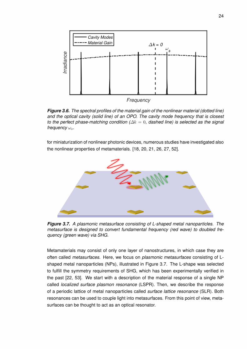
is much larger than the linewidth ∆νc and the free spectral range ∆νfsr of the cavity.Thus, there are several values for ωs with high enough material gain that can be coupledinto the cavity. However, only the ωs closest to the perfect phase-matching condition, i.e.∆k = 0, is strongly enhanced and is selected as the output frequency. As the cavitymode frequencies depend on the cavity, ωs can be accurately tuned by changing thecavity length.[3]

OPOs are widely used as tunable laser sources in ultraviolet, visible and infrared re-gions. They are used to produce nano-, pico- and femtosecond laser pulses as well ascontinuous-wave lasers. [50, 51] In this Thesis, however, we are not using an OPO as alight source. We are more interested in the operating principles of an OPO which we willapply to some extent in our sample design.

3.3 Metasurfaces

Metamaterials are artificial materials consisting of nanoscale structures such as metalnanoparticles or dielectric gratings. They can exhibit optical properties that are not foundin nature such as strong optical activity, epsilon-near-zero behaviour, nano-scale phase-engineering, and magnetism at optical frequencies [10–15]. Due to the growing demand

24

Frequency

Irra

dia

nce

Cavity Modes

Material Gaink = 0

s

Figure 3.6. The spectral profiles of the material gain of the nonlinear material (dotted line)and the optical cavity (solid line) of an OPO. The cavity mode frequency that is closestto the perfect phase-matching condition (∆k = 0, dashed line) is selected as the signalfrequency ωs.

for miniaturization of nonlinear photonic devices, numerous studies have investigated alsothe nonlinear properties of metamaterials. [18, 20, 21, 26, 27, 52].

Figure 3.7. A plasmonic metasurface consisting of L-shaped metal nanoparticles. Themetasurface is designed to convert fundamental frequency (red wave) to doubled fre-quency (green wave) via SHG.

Metamaterials may consist of only one layer of nanostructures, in which case they areoften called metasurfaces. Here, we focus on plasmonic metasurfaces consisting of L-shaped metal nanoparticles (NPs), illustrated in Figure 3.7. The L-shape was selectedto fulfill the symmetry requirements of SHG, which has been experimentally verified inthe past [22, 53]. We start with a description of the material response of a single NPcalled localized surface plasmon resonance (LSPR). Then, we describe the responseof a periodic lattice of metal nanoparticles called surface lattice resonance (SLR). Bothresonances can be used to couple light into metasurfaces. From this point of view, meta-surfaces can be thought to act as an optical resonator.

25

3.3.1 Localized Surface Plasmon Resonance

The optical properties of metals are governed by their electronic structure. The mostcommon model to understand the properties of metals is the free electron gas modelwhere valence electrons are assumed to move freely between positively charged metalions [54]. Therefore, metals to conduct heat and electric charge better than most solids,and due to this fact these electron are called conduction electrons. When a metal is illu-minated with light, the electromagnetic interactions induce oscillations in the conductionelectrons. The oscillations are called plasmons, and they have a specific frequency calledplasmon frequency. When the incident light and plasmons are in resonance, the light iscoupled into the metal structure causing an electronic excitation. In NPs, the excitationis restricted to the particle dimensions, and thus the particle exerts an effective restoringforce on the oscillating particles which enhances the local electric field near the particle.This resonance is LSPR and it occurs at the resonance wavelength λ0. [36]

+ -

-

+ +

(a) (b)

y

x

Figure 3.8. The current distributions associated with effective electric dipoles in an L-shaped metal nanoparticle for (a) x-polarized and (b) y-polarized incident light [23]. Theassociated local fields give rise to LSPRs. Here, the resonance wavelength is longer forx-polarized than for y-polarized light.

The spectral location of LSPR, i.e. value of λ0 depends on many parameters. Firstof all, the choice of material affects λ0 significantly. For example, silver has typicallyshorter resonance wavelength than gold [55]. Second, the particle size impacts as well,as λ0 increases monotonically with particle dimensions. Connected to the previous, thepolarization of the incident light also has an impact on λ0. The induced dipoles areparallel to the incident polarization, and thus the resulting electric current follows a pathin the particle that connects the two poles of the induced dipole (marked with black arrowsin Figure 3.8). Now, λ0 increases with the length of the mentioned path. Therefore for L-shaped NPs, λ0 is larger for the x-polarized incident light than for the y-polarized incidentlight. Finally, the refractive index of the surrounding medium and the neighbouring NPsalso have a shifting impact on λ0.[36] The inter-particle coupling of plasmons can alsoimpact the resonance linewidth, as was demonstrated by Czaplicki et al. [27]. Next, wewill describe the impact of the efficient inter-particle coupling in a periodic metasurfaceillustrated in Figure 3.9.

26

3.3.2 Surface Lattice Resonance

When NPs are organized in a periodic lattice, they act as a diffraction grating. The incidentlight is then diffracted from the grating in accordance with equation [25]

nsub sin(βi) = nsup sin(θ)± iλp, (3.15)

where i is the diffraction order, λ is the wavelength of the incident beam, p is the gratingperiod, θ is the incident angle, and nsub and nsup are the refractive indices of transmitted(substrate) and incident (superstrate) medium, respectively. In typical experiments, thetuned θ is the incident angle in air. Then, according to Snell’s law, we can set nsup = 1

even if the grating is covered with a superstrate material.

At a certain wavelength or a certain incident angle, the diffracted wave starts to propagatealong the grating surface, i.e. βi = 90°. Then, the induced dipoles in NPs start to coupleefficiently giving a rise to a collective response known as a SLR. The spectral features ofSLRs, also known as Rayleigh anomalies, can be extremely narrow and sensitive whichmakes them ideal for e.g.sensing applications. Furthermore, the grating material itselfdoes not impact the diffraction from the grating. Thus, also fully dielectric structuresexhibit resonances similar to SLRs that are called guided-mode resonances (GMR) [56–59].

We can now rewrite Equation (3.15) and derive an equation for the spectral location of aSLR as [60]

λi = p

(nsub

|i|− sin(θ)

i

). (3.16)

It is worth mentioning that SLRs arise only if the incident light is polarized perpendicularto the grating period. As much is illustrated in Figure 3.9 where two SLR modes of aplasmonic metasurface propagate in the direction perpendicular to their polarization.

py

px

SLRx

SLRy

y

x

z

Figure 3.9. Surface lattice resonance modes for a periodic plasmonic metasurface.When light is polarized along either x- or y-coordinate, the resonance wavelengths de-pend on the lattice constant (py or px) perpendicular to the polarization.

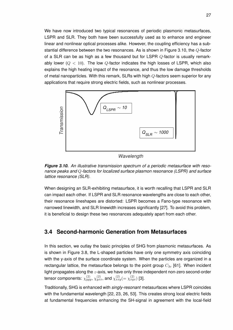
27

We have now introduced two typical resonances of periodic plasmonic metasurfaces,LSPR and SLR. They both have been successfully used as to enhance and engineerlinear and nonlinear optical processes alike. However, the coupling efficiency has a sub-stantial difference between the two resonances. As is shown in Figure 3.10, the Q-factorof a SLR can be as high as a few thousand but for LSPR Q-factor is usually remark-ably lower (Q < 10). The low Q-factor indicates the high losses of LSPR, which alsoexplains the high heating impact of the resonance, and thus the low damage thresholdsof metal nanoparticles. With this remark, SLRs with high Q-factors seem superior for anyapplications that require strong electric fields, such as nonlinear processes.

Wavelength

Tra

nsm

issio

n QLSPR

10

QSLR

1000

Figure 3.10. An illustrative transmission spectrum of a periodic metasurface with reso-nance peaks and Q-factors for localized surface plasmon resonance (LSPR) and surfacelattice resonance (SLR).

When designing an SLR-exhibiting metasurface, it is worth recalling that LSPR and SLRcan impact each other. If LSPR and SLR resonance wavelengths are close to each other,their resonance lineshapes are distorted: LSPR becomes a Fano-type resonance withnarrowed linewidth, and SLR linewidth increases significantly [27]. To avoid this problem,it is beneficial to design these two resonances adequately apart from each other.

3.4 Second-harmonic Generation from Metasurfaces

In this section, we outlay the basic principles of SHG from plasmonic metasurfaces. Asis shown in Figure 3.8, the L-shaped particles have only one symmetry axis coincidingwith the y-axis of the surface coordinate system. When the particles are organized in arectangular lattice, the metasurface belongs to the point group C3v [61]. When incidentlight propagates along the z-axis, we have only three independent non-zero second-ordertensor components: χ(2)

yyy, χ(2)yxx, and χ

(2)xxy(= χ

(2)xyx) [3].

Traditionally, SHG is enhanced with singly-resonant metasurfaces where LSPR coincideswith the fundamental wavelength [22, 23, 26, 53]. This creates strong local electric fieldsat fundamental frequencies enhancing the SH-signal in agreement with the local-field

28

model described in Section 2.9. The singly-resonant use of SLR has also been experi-mentally demonstrated for dielectric and plasmonic metamaterials alike [19, 62]. In thelatter, the SH-enhancement is far greater with SLRs than with LSPRs, when compared tothe off-resonance signal. When we compare the linewidths of these two resonances andconsider the Miller’s rule (2.53), this result is quite expected.

An experimental study performed by Celebrano et al. [63] shows that SH-signal can beimproved even further with multiresonant metamaterials. In a multiresonant design, ma-terial resonances occur both the fundamental and at the SH-wavelengths which, againfollowing the local-field model, enhances the SH-signal. However, the utilization of mul-tiresonant design requires that the fundamental and SH-fields have orthogonal polariza-tions which then connects the SH-signal to the tensor component χ(2)

yxx. In recent numer-ical studies [28, 64], Huttunen et al. demonstrate multiresonant sample designs whichutilize several SLRs and could achieve reasonable conversion efficiencies with second-and third-order processes.

(a) (b)Miller's rule NLST

(2) P(2ω)

(1)(3)

Figure 3.11. Two methods to evaluate the nonlinear response of plasmonic metasur-faces. (a) Miller’s rule consists of evaluation of the linear properties at fundamental andsecond-harmonic wavelengths. (b) Nonlinear scattering theory (NLST) has three evalua-tion steps: (1) The excitation by the fundamental field; (2) calculation of SH-polarization;and (3) the evaluation of the overlap integral between the SH-polarization and the local-field induced by a wave propagating from the detector and oscillating at the SH-frequency.

Even though the Miller’s rule predicts correctly superiority of SLR over LSPR, it is notaccurate enough to describe nonlinear responses of metasurfaces [65, 66]. Instead, thenonlinear scattering theory (NLST) [67], illustrated in Figure 3.11, should be used. NLSTevaluates the SH-emission Enl(2ω) with three steps. The first step is the material excita-tion by the fundamental field. The second step is the calculation of the SH-polarization.As a final step, we evaluate the overlap integral be between SH-polarization and the local-field induced by a wave propagating from the detector and oscillating at the SH-frequency.Then, the SH-emission is evaluated by using the following overlap integral:

Enl(2ω) ∝∫∫

χ(2)E2(ω)E(2ω)dS, (3.17)

where dS indicates the integration over the metasurface. E(ω) and E(2ω) are dependenton the local-fields at the fundamental and SH frequencies, respectively.

29

4 RESONANT WAVEGUIDE GRATINGS

In this chapter, we demonstrate proof-of-principle studies performed on fully dielectricresonant waveguide gratings (RWGs) made from silicon nitride (SiN). We start with adescription of our samples and measurement conditions. Then, we will describe the ex-perimental setup used for the linear and nonlinear measurements. Next, we will explainthe simulation methods used to estimate the second-harmonic response of our RWGs.In the second and third sections, we demonstrate a clear agreement between our sim-ulations and experiments. We start by comparing the simulated and measured linearproperties of our RWGs. Then, we present our results for the measured and simulatedSH emission from our samples. We conclude this chapter with the evaluation of oursimulation methods and with some proposals for future studies.

4.1 Samples and Research Methods

The RWGs studied here consisted of SiN. We used ion-beam-sputtering (IBS) [68] tofabricate 90–100 nm thick SiN gratings (ng = 1.9) on fused silica (ns = 1.457) and tocover them with silicon dioxide (SiO2 , nc = 1.49). Here, we set the grating periods p

of our samples to 500 and 600 nm and labelled them accordingly as S500 and S600.The widths of the SiN grooves in the RWGs were half of the grating period, and thus,both samples had the same amount of active material (SiN). The differences in opticalproperties should then be a consequence of the different grating periods. An illustrativedrawing of a SiN RWG is shown in Figure 4.1.

a

p

ng

ns

θ

d

nc

Figure 4.1. Schematic drawing of a resonant waveguide grating made of silicon nitride(SiN, ng = 1.9). The gratings are fabricated on fused silica (ns = 1.457) and covered witha silicon dioxide cladding (SiO2, nc = 1.49). SiN lines have thickness d = 90 – 100 nm,and width a which is half of the grating period p. The grating is illuminated with laser lightcentered at wavelength λ = 1064 nm at an incident angle θ.

30

As is shown in Figure 4.1, our RWGs are centrosymmetric. In order to fulfill the symmetryrequirements for SHG, the incident angle θ had to be tuned. The tuning of the incidentangle helps us to efficiently excite GMRs, as they are also angle dependent (see Equation(3.16)). Now, it is useful to rewrite Equation (3.16) for the first-order (i = ±1) resonanceangles as

θ±1 = asin

(±(ns −

λ

p

)), (4.1)

where wavelength λ is set to 1064 nm. In this case, the first-order RAs appear at the inci-dent angles of 42.5° and 18.6° for p = 500 nm and 600 nm, respectively. The wavelength–angle correspondence for the first-order RAs is illustrated in Figure 4.2.

0 10 20 30 40 50 60

Incident angle (degrees)

200

400

600

800

1000

1200

1400

Wavele

ngth

(nm

)

S500, i = -1

S500, i = 1

S600, i = -1

S600, i = 1

1064 nm

532 nm

Figure 4.2. The resonance wavelength as the function of the incident angle for the first-order RAs. For fundamental wavelength of 1064 nm (red dashed line), the RA angles oforder i = –1 are 42.5° and 18.6° for samples S500 and S600, respectively. The corre-sponding angles for RAs of order i = 1 at SH wavelength of 532 nm (green dashed line)are 22.7° and 34.2°.

In order to measure the transmittance and SH response of our RWGs, we used the setupillustrated in Figure 4.3. As a light source, we used a pulsed Nd:YAG (Ekspla PL 2200)laser with a wavelength of 1064 nm, pulse duration of 60 ps and a repetition rate of 1 kHz.To avoid possible sample damage, we limited the input power of the laser to 3 mW with ahalf-wave plate (HWP) and a linear polarizer (LP). In order to efficiently excite GMRs, wethen used another HWP to set the polarization along the SiN lines of the RWGs. Then,another LP was used to select the correct polarization of the generated SH signal. Toensure efficient coupling to the GMR modes, the laser beam as weakly focused on thesample using a lens with a focal length f = 400 mm. The sample itself was placed ona rotating stage allowing us to measure the transmittance and the SHG as the functionsof the incident angle. Furthermore, we put the sample between a long-pass filter (LPF)and a short-pass filter (SPF). This ensured that the detected SHG emission was onlydue to the sample emission. As the SH responses of nanoscale structures are typicallyvery weak, we used a photomultiplier tube (PMT) to detect the SH signal. In linear mea-surements, we turned LPF aside and used a photodiode to measure transmission of the

31

fundamental wavelength 1064 nm.

Nd:YAG Laser1064 nm

60 ps @ 1 kHz HWP1 LP1L1 L2LPF SPFHWP2 PD orPMT

Sample LP2

Figure 4.3. Schematic drawing of the experimental setup. The focal lengths of the lensesare 400 mm (L1) and 50 mm (L2). HWP = Half-wave plate, LP = Linear polarizer, LPF= Long-pass filter and SPF = Short-pass filter. The sample was put on a rotating stageallowing us to change the incident angle. In the nonlinear measurements, the SH sig-nal was collected using a photomultiplier tube (PMT). In linear measurements, SPF wasturned aside and the transmission was measured with a photodiode (PD).

In order to connect the nonlinear scattering theory (NLST) to the experiments, we alsoperformed numerical simulations based on our RWGs. We performed the first part of oursimulations using a commercial Lumerical FDTD Solutions software which uses the finite-domain time-domain (FDTD) [69] method to evaluate electromagnetic fields present in thestructure. We performed two-dimensional simulations for a structure illustrated in Figure4.1. As an excitation source in our simulations, we used a plane wave with a wavelengthof 1064 nm which we polarized along the SiN grooves. To gather the required data for thecalculation based on the NLST, we used three monitors in our simulation system. Onemonitor measured transmission T of fundamental light.The other two measured electricfield profiles Efund and ESH near the SiN gratings at the fundamental and SH wave-lengths, respectively. By performing an angle sweep, we gained values for T , Efund andESH as the functions of the incident angle θ. Then, we inserted the gained field profilesto Equation (3.17) and got an estimation for the scattered SH field. By then transformingthe scattered SH field into irradiance we were able to compare the numerical predictionswith the experimental results.

4.2 Linear Properties

We investigated the linear and nonlinear optical properties of SiN RWGs with two differentgrating periods (p = 500 and 600 nm). First, we measured and simulated the transmissionof the fundamental wavelength 1064 nm as a function of the incident angle θ. As is shownin Figure 4.4, we performed experiments over the range θ = 0° – 50° but we limited thesimulation range closer to the theoretical RA angles given by Equation (4.1).

The first glance at Figure 4.4 reveals that the simulations and experiments agree ratheraccurately on the angular locations of the GMRs. The small differences between theoret-ical and experimental values can be plausibly explained by the uncertainties associatedwith the experimental setup. It is also worth mentioning that all resonances correspondto the diffraction order i = –1 and that the resonance angles θexp and θsim decrease withp.

32

(a) (b)

16 18 20 22 24

Incident angle (degrees)

0

20

40

60

80

100

Tra

nsm

issi

on (

%)

S600 Exp.S600 Sim.

38 40 42 44 46

Incident angle (degrees)

0

20

40

60

80

100

Tra

nsm

issi

on (

%)

S500 Exp.S500 Sim.

Figure 4.4. Experimental (solid lines) and simulated (dashed lines) transmission as func-tion of incident angle for samples (a) S500 (red) (b) and S600 (black). The resonanceangles are around 18° and 42° for S500 and S600, respectively.

Another difference between the experimental and simulated results is in the strengths ofthe resonance peaks. The experimental peaks have practically equal amplitudes, which isa rather expected result since both samples have the same amount of SiN. The simulatedtransmission peaks, however, have slightly different amplitudes for our samples. It is thenlikely that our simulations did not cover the most optimal coupling conditions. This impliesthat the spectral simulation resolution was slightly inadequate, especially in the simulationfor S600. However, improving the simulation conditions is quite time consuming andwould, in the end, lead to results with spectral features much narrower than those of thelight sources and fabricated samples used in experimental work.

The mere locations and strengths of the resonance peaks do not offer much informationthat is needed to evaluate the nonlinear properties of our samples. The angular linewidths∆θsim and ∆θexp are more relevant since they are connected to the spectral linewidth byequation

∆λ = p cos(θ)∆θ, (4.2)

and thus, also to the Q-factor through Equation (3.10). As the emitted SH irradiancescales as ISHG ∝ Q4, angular linewidths help us to estimate the SH responses of oursamples. The relevant results of our linear experiments are listed in Table 4.1.

Table 4.1. Linear results for samples S500 and S600. The angle θRA is the theoreticalincident angle of the Rayleigh anomaly, and θsim and θexp are the simulated and experi-mental resonance angles, respectively. ∆θsim and ∆θexp are the angular linewidths andQsim and Qexp are the Q-factors of the simulated and measured resonances, respectively.

Sample θRA θsim θexp ∆θsim ∆θexp Qsim Qexp

S500 42.5° 42.4° 41.7° 0.1° 0.4° 1650 410S600 18.6° 19.5° 17.5° 0.1° 0.3° 1080 350

33

The experimental linewidths ∆θexp are significantly larger than their simulated counter-parts ∆θsim. This is most likely a consequence of the differences between the lightsources used in simulations and experiments. In the simulations, the light source is aperfect plane wave without divergence, while the laser beam used in the experimentshas a slight divergence. The experimental Q-factors are thus reduced when comparedwith the Q-factors of the simulation results. When we compare these results against thepredictions based on the Miller’s rule, the GMR-enhanced SHG would be stronger forS500 based on experiments and simulations alike. Since the SH emission scales asISHG ∝ Q4, the experimental Q-factors now imply that S500 should have three timesstronger SH response than S600. Alternatively, based on simulated Q-factors, the SH-response of S500 should be seven-fold to the response of S600.

4.3 Second-harmonic Generation from Resonant WaveguideGratings

Next, we studied the SH response of our samples using the setup shown in Figure 4.3.We performed measurements over incident angles θ = 0° – 70° and obtained the resultsplotted in Figure 4.5. The values for the emitted SH power shown in the graph are roughestimations due to the inaccuracies of our detection devices. First, the noise levels ofour PMT might vary significantly between the measurements. Moreover, the power meterused for power calibration had a noise level of the order of 10 fW. Combined, theseinaccuracies result in error terms up to 30 fW for our experiments. Nevertheless, theorder-of-magnitude should be correct, and thus we estimate conversion factors on theorder of 10-11 for both samples.

0 10 20 30 40 50 60 70

Incident angle (degrees)

0

50

100

150

SH

G (

fW)

S500

S600

650

100

Figure 4.5. Measured SH power as a function of incident angle for samples S500 (red)and S600 (black). The strongest signals are measured at the experimental resonance an-gles defined in the transmission measurements. The resonance enhancement comparedwith the off-resonance signals are 650 and 100 for S500 and S600, respectively.

34

The results shown in Figure 4.5 further confirm that the GMRs enhance the local fieldspresent in the SiN RWG. coincide well with the measured resonance angles, and are devi-ated only by around 0.1°. The linewidths of the SH peaks are also equal to the linewidths∆θexp of the SLR peaks. As was expected based on the measured Q-factors, S500 hasa SH response that is roughly four times stronger than the emitted SH power of S600.However, this relation may be inaccurate since the absolute values for the emitted powermay slightly vary between separate measurements. Another, and possibly more accuratemethod to evaluate the role of the resonance enhancement would be to compare theresonant signals with the off-resonance signals, illustrated with double arrows in Figure4.5. These enhancements are 650 and 100 for S500 and S600, respectively. This resultagrees rather well with the simulated Q-factors based on which we estimated a seven-folddifference between the two samples. Considering the results so far, we conclude that thesimulations define the linear properties accurately.

In order to validate the NLST method as a reliable basis for simulation, we need to con-sider our results beyond the simulated Q-factors. The incident light induces dipole mo-ments into the SiN grating that are then amplified by the propagating GMR mode. Thisgives rise to the local fields at the fundamental wavelength, and according to NLST, alsoto the SH emission. As is shown in Figure 4.6, the local field has a 12-fold increase at theresonance angle (42.4° for S500) when compared with the off-resonance electric field.For S600, the local-field enhancement is roughly ten-fold and occurs at the simulatedresonance angle 19.5°. For the vacuum field term in Equation (3.17), we also simulatedlocal fields at the SH wavelength. As the first-order RA-angles for λ = 1064 nm and λ =

532 nm differ quite significantly for both of our samples (see Figure 4.2), the local field atλ = 532 nm remains constant over the simulated angles.

41.5 42 42.5 43

Incidence angle (degrees)

50

60

70

80

90

100

Tra

nsm

issio

n %

0

5

10

15

Efu

nd (

a.u

.)

Figure 4.6. Simulated transmission and the local electric field Efund for the sample S500.The local electric field is normalized to the field amplitude next to the resonance. At theresonance angle 42.4°, the local field is 14-fold when compared with the off-resonancefield.

Next, we inserted the gained field profiles at the fundamental and SH wavelength to

35

the Equation (3.17). From there, we obtained simulated angle-dependence for the SHpower emitted from our RWG structures. For visual comparison between simulated andexperimental results, shown in Figure 4.7, we normalized all data sets to the maximumvalue of each individual set. We can then compare the resonance enhancements andpeak locations of simulation with the experimental results.

(a) (b)

40 42 44 46

Incident angle (degrees)

0

0.2

0.4

0.6

0.8

1

SH

G (

a.u.

)

S500 Exp.S500 Sim.

1000

16 18 20 22 24

Incident angle (degrees)

0

0.2

0.4

0.6

0.8

1

SH

G (

a.u.

)

S600 Exp.S600 Sim.

150

Figure 4.7. Emitted SHG signal based on the experiments (solid lines) and simulations(dashed lines) for samples (a) S500 and (b) S600. The signal enhancements comparedto the off-resonant values are 1000 and 150 for S500 nm and S600, respectively. All datasets are normalized to the maximum signal of each individual set. Thus, the graphs donot display information about the signal strengths relative to the other sets.

For both samples, the simulated SH emission peaks locate at the same incident anglesand have the same linewidths than the corresponding GMR peaks. This further confirmsthe role of GMR as an effective field-enhancing response. Also, the simulated resonanceenhancement factors agree with the experimental results. Once again, the enhancementfactor of S500 is seven-fold to the factor of S600. This agrees with the Q-factor-basedestimation we made in Section 4.2. Relevant results from SHG measurements and sim-ulations are listed in Table 4.2.

Table 4.2. Nonlinear results for samples S500 and S600. The SH emission peaks lo-cate at the incident angles θsim and θexp for simulations experiments, respectively. Theyhave angular linewidths ∆θsim and ∆θexp. At these resonant angles, the SH emission isenhanced by factors Esim and Eexp in simulations and experiments, respectively.

Sample θsim θexp ∆θsim ∆θexp Esim Eexp

S500 42.4° 41.7° 0.1° 0.4° 1000 650S600 19.5° 17.5° 0.1° 0.3° 150 100

Overall, our results confirm the reliability of FDTD and NLST as simulation methods.Both linear and nonlinear simulations agree with experimental results with adequate ac-curacy. The differences between the experiments and simulations can be explained withthe uncertainties associated with our experimental setup and with the limitations of oursimulations. For example, by improving the collimation of our laser beam, we shouldreach better agreement between the experimental and simulated results.

36

More importantly, our results validate utilizing GMRs as an effective method to engineerand enhance the SHG in dielectric materials. Our results motivate to design fully dielectricstructures suitable for other nonlinear processes such as SPDC, DFG, and cascade third-harmonic generation. The processes could be used to realize nanoscale photon-pairgeneration and light sources opertaing in THz and ultraviolet regions.

37

5 RESONANT PLASMONIC METAMATERIALS

In this chapter, we propose two novel plasmonic metamaterials designed to emit coher-ent photon pairs via SPDC. For both designs, the building blocks are L-shaped aluminumnanoparticles placed in a homogeneous dielectric medium, such as in glass. The firstsample is a multiresonant metasurface exhibiting SLRs both at the pump and the sig-nal wavelengths for orthogonal polarizations. The second sample consists of a singly-resonant metasurface sandwiched between two distributed Bragg reflectors. In this sam-ple, the multiresonant conditions are achieved by coupling the pump wavelength to thecavity mode and the signal wavelength to the SLR. For both designs, we used FDTD andNLST in order to evaluate their SPDC-response.

5.1 Simulation Methods

In order to evaluate different enhancement methods, we simulated SPDC-response oftwo different types of plasmonic metamaterials. Both structures, described in detail later,consisted of L-shaped aluminum nanoparticles embedded in a homogeneous medium(ns = 1.45), visualized in Figure 5.1. The particles had an arm length L = 90 nm, anarm width w = 45 nm and a thickness d = 30 nm. Here, the particle dimensions and thematerial were chose to exhibit LSPRs at lower wavelengths (λLSPR ≤ 600 nm). LSPRswould not then interact with the SLR modes, which ensures the high-quality resonancesat the pump and signal wavelengths. As in many previous studies [22, 23, 26, 27, 53],the L-shape was selected to fulfill the symmetry requirements of second-order nonlinearprocesses making χ

(2)yyy, χ(2)

yxx, and χ(2)xxy(= χ

(2)xyx) the allowed tensor components.

y

x L

w

d

Figure 5.1. L-shaped aluminum nanoparticle used as a building block in our sampledesigns. Particle arm length L = 90 nm, arm width w = 45 nm, and thickness d = 30 nmwere selected for LSPRs to locate at low enough wavelengths (λLSPR ≤ 600 nm).

To evaluate the SPDC response of the sample designs, we used FDTD and NLST in a

38

very similar manner as already described in Chapter 4. We started by simulating trans-mission and local fields at pump and signal wavelengths. Unlike in Chapter 4, we had abroadband plane-wave source at the normal incidence polarized first along x-coordinateand then along the y-coordinate of the sample coordinates. We then used NLST to pre-dict the spectral behaviour of SPDC signals corresponding to the tensor componentsχ(2)yyy, χ(2)

yxx, and χ(2)xxy(= χ

(2)xyx). As SPDC and SHG are each other’s reverse processes,

we could use the same overlap integral as we used in Chapter 4.

5.2 Multiresonant Metasurface

The first sample design, illustrated in Figure 5.2, is a multiresonant metasurface consist-ing of aluminum nanoparticles as described above. The nanoparticles were arranged ina lattice with lattice periods px = 414 nm and py = 828 nm along the x− and y−directionsin the sample coordinates, respectively. Periods px and py were selected to give rise toSLRs at the pump wavelength (λp = 600 nm) and signal wavelength (λs = 1200 nm).

z

px

SLRxSLRy

x

y py

Figure 5.2. Schematic drawing of a multiresonant metasurface consisting of L-shapedaluminum nanopartilces. Periodicities px and py are set so that x-polarized SLR isat signal wavelength (λSLR,x = λs = 1200 nm) and y-polarized at pump wavelength(λSLR,y = λp = 600 nm).

With the selected parameters, the strongest enhancement should occur for the processcorresponding to the tensor component χ

(2)yxx, i.e. to the process where the pump is

y−polarized and signal x−polarized. Multiresonant design would then mimic type I non-linear crystals which are widely used in quantum optics [40]. The relevant sample param-eters and enhancement methods for multiresonant design are listed in Table 5.1.

Table 5.1. Metasurface parameters, the designed signal wavelength λs, enhancementresonances for pump and signal wavelengths, and optimal tensor components for themultiresonant design. Periods px and py are the lattice constants in x- and y-coordinates,respectively.

Sample λs (nm) px (nm) py (nm) pump resonance signal resonance tensorsMR 1200 414 828 SLRy SLRx yxx

As a start for our evaluation, we simulated the transmission spectra for x- and y-polarized

39

incident light. The spectra shown in Figure 5.3 confirms the presence of first-order SLRsat the pump (λp = 600 nm) and signal wavelength (λs = 1200 nm) for y-polarized andx-polarized light, respectively. The x-polarized SLR peak has some noise around it whichindicates slightly divergent simulations. The other sharp spectral features correspondto the higher-order SLRs, which we will not utilize in this Thesis. The broader spectralfeatures correspond to the LSPRs at 600 nm and 500 nm for x- and y-polarized light,respectively. As was designed, LSPRs do not overlap with the first-order SLRs whichconfirms that the particle parameters were correctly designed. However, the particles aretoo small for efficient inter-particle coupling leading to the relatively weak transmissionpeaks.

400 600 800 1000 1200 1400 1600 1800 2000

Wavelength (nm)

80

85

90

95

100

Tra

nsm

issio

n (

%)

x

y

Figure 5.3. Spectral transmission for the multiresonant sample design. With x-polarized(blue) and y-polarized (red) light, we detect sharp SLR peaks at the signal wavelengthλs = 1200 nm and at the pump wavelength λp = 600 nm.

Yet again, the strengths of the resonance peaks are not the most essential informationwhen considering the nonlinear properties of the designed metasurfaces. Rather thespectral linewidths ∆λ and the corresponding Q-factors are more relevant. From thespectra in Figure 5.3 we observe that ∆λ are roughly 2 nm for both polarizations leadingto Q-factors of 430 and 550 for y- and x-polarized light, respectively. For y-polarization,the resonance peak is broadened due to mode coupling with the LSPR. This point illus-trates well that it would be difficult to design SLRs to occur at shorter wavelengths thanconsidered here. The LSPRs do not impact the x-polarized resonance peak, but it still hasthe same linewidth of 2 nm and noise around it due to the before mentioned simulationdivergence.

The next step in our simulations was to compute local-field enhancements Eloc,p andEloc,s at the pump and signal wavelengths, respectively. As is shown in Figure 5.4, thespectral behaviours of the field profiles confirms that the local fields are considerablyenhanced due to SLRs. At the signal wavelength, the local electric field is constant for y-polarized light, while for x-polarized light a strong peak occurs at 1200 nm. Here, one canagain see the impact of diverged simulations as small oscillations around the resonance.

40

(a) (b)

590 595 600 605 610

Wavelength (nm)

0

10

20

30

Ele

ctric

fiel

d (a

.u.)

xy

1180 1190 1200 1210 1220

Wavelength (nm)

0

10

20

30

Ele

ctric

fiel

d (a

.u.)

xy

Figure 5.4. Normalized local electric fields close to the (a) pump wavelength λp = 600nm and (b) to the signal wavelength λs = 1200 nm. The local fields are SLR-enhancedwith y-polarized (red) and x-polarized (blue) incident light at λp and λs, respectively.

Close to the pump wavelength, the spectral behaviour of the local field is different. Fory-polarized input, a strong resonance peak locates at 600 nm, and the impact of a higher-order SLR is noticeable at the shorter wavelengths. The x-polarized light gives rise to theLSPR at these wavelengths. Consequently, SLR acts as a damping resonance, whichcan be seen as a dip in the local field at 600 nm.

From the results listed in Table 5.2, we can now predict the SPDC responses correspond-ing to different tensor components. Based on the Miller’s rule and the estimated Q-factors,or by using the NLST method and subsequent local field analysis, χ(2)

yxx should result inthe strongest signal of the three components as it utilizes the multiresonant conditionsmost efficiently. Consequently, the other two should give rise to a much weaker responsesince they utilize only one of the SLRs.

Table 5.2. Simulated results for the multiresonant metasurface with x- and y-polarizedlight sources. The wavelength λ, the linewidth ∆λ, and Q-factor for the utilized SLRs.Eloc,p and Eloc,s are the normalized local field factors at the pump and signal wavelengths,respectively.

Polarization λ (nm) ∆λ (nm) Q Eloc,p Eloc,s

y 602.8 1.4 430 26 5x 1203.8 2.2 550 2 20

As a next step, we used NSLT to evaluate the SPDC response of our metasurface. Wecalculated the responses over the signal wavelength band of 1180–1220 nm, and studiedonly the generation of photon pairs with equal wavelengths. The results were normal-ized to the signal peak of the least efficient process corresponding to χ

(2)xxy(= χ

(2)xyx). As

was expected based on linear results, and is shown in Figure 5.5, the strongest signalcorresponds to χ

(2)yxx and is roughly 400 times stronger than the peak of the weakest sig-

nal. The signal corresponding to χ(2)yyy is only slightly stronger (four-fold) than the one

corresponding to χ(2)xxy.

41

The spectral locations of the peaks also illustrate the impact of SLR on the photon-pairgeneration. For χ(2)

yyy, where all fields are y-polarized, only the local field at λp = 603 nmis enhanced by the SLR, and thus the strongest signal is generated at λ = 1206 nm.Similarly for χ(2)

xyx, only the x-polarized signal field is enhanced by the SLR, and thus thesignal peak is located at λs = 1203 nm. As mentioned before, the process of χ(2)

yxx utilizesSLRs at both pump and signal wavelength resulting in the strongest response of the threeallowed processes. The overlap between Eloc,p and Eloc,s then shifts the signal peak to1205 nm, since y-polarized SLR wavelength (603 nm) is not exactly half of the x-polarizedSLR wavelength (1204 nm). This result implies, that by iteratively improving the design inorder to better spectrally overlap the two SLRs, even stronger signal enhancement couldbe expected.

(a) (b)

1180 1190 1200 1210 1220

Wavelength (nm)

0

1

2

3

4

5

SP

DC

(a.

u.)

yyyxxy

1180 1190 1200 1210 1220

Wavelength (nm)

0

100

200

300

400

500

SP

DC

(a.

u.)

yxx

Figure 5.5. Spontaneous parametric down-conversion (SPDC) as a function of the signalwavelength. The signals illustrated with (a) red, (b) black and blue curves correspond toprocesses described by the tensor components χ

(2)yxx, χ(2)

yyy, and χ(2)xxy(= χ

(2)xyx), respec-

tively. The responses are normalized to the weakest signal peak in our simulation band.

When considering quantum optics and other applications of coherent photon pairs, ourresults here are quite two sided. On the other hand, the relatively narrow linewidths(∼2 nm) of our signal bands illustrate the high coherence of the generated photon pairs.Furthermore, our results suggest that y-polarized illumination on our sample would resultin an efficient generation of x-polarized photon pairs. Thus, the metasurface mimics atype I nonlinear crystal commonly used in quantum optics. On the other hand, however,the process corresponding to χ

(2)xyx would be most useful for quantum optics, since it would

result in the generation of an entangled photon pair with orthogonal polarizations. Forthis process, the multiresonant design is not beneficial but rather disadvantageous even.It would be more useful to utilize singly-resonant conditions where the SLRs enhancethe signal fields for both polarizations. However, this would require other enhancementmethods for the pump wavelength. As one solution, we propose utilization of a DBRcavity, which we demonstrate in the next section.

42

5.3 Singly-resonant Metasurface in Bragg Cavity

As the second option, we studied a singly-resonant-in-cavity (SRC) design, shown in Fig-ure 5.6. Here, a singly-resonant metasurface, consisting of the same aluminum nanopar-ticles as the earlier sample design, is placed in the center of a DBR cavity. Now, thenanoparticles are arranged in a square lattice (px = py = 793 nm) giving a rise to a SLRat λs = 1150 nm for both x- and y- polarized light. The DBRs consist of ten layer pairsof titanium dioxide (TiO2, n = 2.5) and silicon dioxide (SiO2, n = 1.45), and they aredesigned to reflect light around λB = 550 nm.

λc=λSLR/2

L=8λc

......

y

x

z

px

pySLRxSLRy

Figure 5.6. Schematic drawing of a sample consisting of a DBR cavity and a singly-resonant metasurface. DBRs are formed with ten layer pairs of titanium dioxide (TiO2,n = 2.5) and silicon dioxide (SiO2, n = 1.45) and they are designed to reflect light aroundλB = 550 nm. The DBR cavity is used to enhance the field at the pump wavelength(λc = λp = 575 nm) and SLRs are used to enhance the local field at signal wavelength(λSLR = λs = 1150 nm).

Unlike the typical DBR cavities, we selected our cavity wavelength λc = λp = 575 nmto differ from λB = 550 nm. This selection helped us to have lossless propagation forthe generated signal and to avoid overlapping of SLR-peaks with the DBR-transmissionsidebands. Therefore, we should obtain strong local field enhancements close to themetasurface using cavity coupling and SLRs at λp and λs, respectively. Since the op-eration of the DBR is independent of the input polarization, and SLRs have the samewavelength for x- and y-polarized light, the SRC design should give equal enhancementfor all allowed second-order tensor components. In theory, SRC design could then mimiccrystal types 0, I and II, which is a clear advantage over the conventional phase-matchedmaterials. χ

(2)xxy = χ

(2)xyx is especially a subject of interest since it corresponds to the

process where the generated photons have orthogonal polarizations. Now, we can listrelevant sample parameters and enhancement methods for the SRC sample design inTable 5.3.

Like in the previous simulations, we started by defining the linear properties with FDTD.The transmission spectrum shown in Figure 5.7 is very similar to the typical transmissionspectrum of a uniform DBR (see Figure 3.3). The wide reflection region around λB =

550 nm and the strong sidebands (marked with black arrows in Figure 5.7) are the con-sequences of a relatively small number of layer pairs and the high difference between the

43

Table 5.3. Metasurface parameters, the designed signal wavelength λs, enhancementresonances for pump and signal wavelengths, and optimal tensor components for singly-resonant-in-cavity (SRC) design. Periods px and py are the lattice constants in x- andy-coordinates, respectively.

Sample λs (nm) px (nm) py (nm) pump resonance signal resonance tensorsSRC 1150 793 793 cavity mode SLRy, SLRx xxy, yxx, yyy

refractive indexes of TiO2 (n = 2.5) and SiO2 (n = 1.45). There are many methods tomake the reflection band narrower and to reduce the strengths of the sidebands, but theyare beyond the scope of this Thesis. Here, we are more interested in the properties ofthe cavity and the metasurface.

500 700 900 1100 1300

Wavelength (nm)

0

20

40

60

80

100

Tra

nsm

issi

on (

%)

Sidebands

Figure 5.7. Transmission spectrum of the SRC design. A SLR peak is detected at 1168nm, marked with the red circle, otherwise the spectrum looks typical for a uniform DBR.Here, the sidebands typical for an uniform DBR are marked with black arrows. There isalso a small transmission peak at 583 nm, marked with the green circle, but due to thescaling of the y-axis it is not visible here.

The spectrum in Figure 5.7 shows the influences of the cavity modes and the SLR. Theresonance peak for cavity mode locates at λ = 583 nm while the SLR peak is seen atλ = 1168 nm. The resonance wavelengths differ slightly from the designed values. Fortu-nately, they differ roughly by a factor of two, and thus we should still get the multiresonantconditions fulfilled for SPDC. Furthermore, peaks have relatively low amplitudes, andthus, they are re-plotted for clarity in Figure 5.8. We also note that the spectra for x- andy-polarized light are almost identical, as was intended. We can thus limit our visualizationto the x-polarized input.

Now, we can again estimate the linewidths and Q-factors of our resonances. The cavityresonance at 583 nm has the linewidth ∆λ = 0.12 nm and thus Q-factor of value 4850.For the SLR at 1168 nm, the corresponding values are ∆λ = 0.35 nm and Q = 3340.These Q-factors are now an order-of-magnitude larger than the SLR Q-factors of the pre-vious design. However, this is a consequence of a higher simulation resolution required

44

for the SRC simulations.

(a) (b)

1130 1140 1150 1160 1170

Wavelength (nm)

85

90

95

100

Tra

nsm

issi

on (

%)

565 570 575 580 585

Wavelength (nm)

0

0.1

0.2

0.3

Tra

nsm

issi

on (

%)

Figure 5.8. Transmission spectrum of the SRC design close to (a) the pump wavelengthand (b) signal wavelength. The cavity mode resonance is detected as a peak in thespectrum at 538 nm, and the SLR as a dip at 1168 nm.

The next step in our study was, yet again, the evaluation of the local field profiles visual-ized in Figure 5.9. As was expected , the field profiles, which are again normalized to theincident field, have very narrow spectral features at the resonance wavelengths. The SLRinduced enhancement is of similar strength than with multiresonant design (see Figure5.4). Same can not be said for the local field at the cavity resonance, which is surprisinglylow. This might result from slightly inaccurate simulations, which also impacts the ampli-tude and the Q-factor of the resonance peak. For example, the Q-factor of a FP etalonwith our cavity length should be roughly ten times larger to the simulated value. Keepingthis in mind, we continue our evaluation with the relevant linear properties listed in Table5.4.

(a) (b)

1130 1140 1150 1160 1170

Wavelength (nm)

0

5

10

15

20

25

Ele

ctric

fiel

d (a

.u.)

565 570 575 580 585

Wavelength (nm)

0

0.5

1

1.5

2

2.5

Ele

ctric

fiel

d (a

.u.)

Figure 5.9. Normalized local electric fields in the SRC design close to (a) the pumpwavelength and (b) signal wavelength.

Next, we applied NLST methodology to calculate the SPDC spectrum shown in Figure5.10. Unlike the SPDC spectrum for the multiresonant design, there are now two dis-

45

Table 5.4. Simulation results for the cavity mode resonance and SLR for the SRC design.The resonances locate at wavelengths λ, have linewidths ∆λ, quality factors Q and themaximum local field enhancement factors Eloc.

Resonance λ (nm) ∆λ (nm) Q Eloc

Cavity mode 583 0.12 4850 2.5SLR 1168 0.35 3340 21

tinguishable and narrow peaks. The stronger peak locates at the SLR wavelength 1168nm and the other, a slightly weaker peak at 1165 nm, which is exactly twice the cavitymode wavelength. This once again illustrates the enhancing impact of high-Q-factor res-onances. The fact that there are two peaks is the consequence of the overlap integralthat is being used in the NLST method to estimate the signal strength. The linewidthsof the two resonance peaks are so narrow that they do not properly overlap. Thus, thesignal is enhanced at two separate wavelengths instead of one. By better overlappingbetween these two resonances, we should have only one signal peak with a dramaticallylarger enhancement factor.

1130 1135 1140 1145 1150 1155 1160 1165 1170

Wavelength (nm)

0

1

2

3

4

5

6

SP

DC

(a.u

.)

104

Cavity mode

SLR

Figure 5.10. Spontaneous parametric down-conversion spectrum of the SRC design.The emission peaks at 1165 nm and 1168 nm result from field enhancements by couplingto the cavity mode and SLR mode, respectively.

When considering the local-field enhancements listed in Table 5.4, the two peak ampli-tudes are surprisingly close to each other. Especially when we recall that SLR enhancestwo of the relevant fields, while the cavity mode enhances only one. Here, it is worthrecalling that the values listed Table 5.4 are for the single unit volume, where the fieldwas at maximum. Moreover, the overlap integral of NLST covers the whole simulationvolume. SLR indeed creates a stronger local field near the nanoparticles. However, thecoupling into the cavity mode causes an equally strong field over the whole simulationvolume. Therefore, the cavity mode enhancement is of the same order-of-magnitudethan the SLR enhancement.

46

Again, it is worth to mention that the SPDC spectrum is very close to the one shown inFigure 5.10 for all allowed tensor components. Thus, we display only the results corre-sponding to χ

(2)xxy = χ

(2)xyx (type II process) since it is the most useful for applications in

quantum optics. We also note that the two other processes, corresponding to χ(2)yyy (type

0) and χ(2)yxx (type I), would be more useful for SHG. This multi-functionality, however, was

designed and is the main advantage of the SRC design over the multiresonant design.

47

6 CONCLUSION

In this Thesis, we demonstrated how the utilization of high-quality-factor resonancesimproves the nonlinear optical properties of metamaterials. Here, we focused on twosecond-order processes: Second-harmonic generation (SHG) and spontaneous para-metric down-conversion (SPDC). We successfully performed experiments that confirmthe impact of high-quality-factor resonances and also validate our simulation methods.We then proceeded to design two novel plasmonic metamaterial structures that rely ontwo types of high-quality-factor resonances.The first resonance is a collective responseof periodic structures known as surface lattice resonance (SLR) and guided-mode reso-nance (GMR) in plasmonic and dielectric metamaterials, respectively. The second reso-nance rises from the coupling of the incident light into an optical cavity.

First, we characterized linear and nonlinear optical properties of fully dielectric resonantwaveguide gratings (RWGs) made of silicon nitride. We studied two RWGs with differentgrating periods and noticed the enhancing impact of GMRs with both samples. In thetransmission spectra, we detected narrow spectral features at predicted locations withrelatively high Q-factors of ∼ 400. At the same spectral locations, we measured strong SHresponses with up to 650-fold enhancement when compared against the off-resonancesignal.

Next, we used the finite-difference time-domain (FDTD) method to simulate the linearproperties of our RWGs. The simulated transmission spectra had GMR peaks close tothe experimental locations with Q-factors up to 1600. With FDTD we also simulated thelocal fields at fundamental and SH wavelength on the grating surfaces. Then based onnonlinear scattering theory (NLST), we used the simulated field profiles to numericallyevaluate SH emission from our samples. Now, the SH emission was up to 1000-foldenhanced when compared against the off-resonance values.

The proof-of-principle studies summarized above confirm two things. First, utilizing GMRsin fully dielectric materials improve their nonlinear properties. In the future, realizing themulti-resonant conditions with GMRs in RWGs could enable the enhancement of othernonlinear processes. For example, realizing cascaded third-harmonic generation couldpave the way towards efficient UV light source in nanoscale. Second, the simulationsagree rather well with experiments validating the chose simulation methods of FDTD andNLST to predict the nonlinear responses of metamaterials. The differences betweenexperiments and simulations can be explained with the inaccuracies of our experimentalsetup. Thus, we can use the presented simulation methods to design metamaterials for

48

future investigations.

Next, we designed two plasmonic metamaterials for efficient SPDC. The basic buildingblocks for both designs were L-shaped aluminum nanoparticles surrounded by a homo-geneous medium, such as glass. This particle symmetry enables three types of SPDCprocesses. One where pump and signal have the same polarization (type 0), one wherethey have orthogonal polarizations (type I), and one where the two signal photons haveorthogonal polarizations (type II). The two latter processes are used in quantum opticsfor coherent photon-pair generation. The SPDC responses were enhanced by design-ing high-quality-factor resonances at both pump and signal wavelengths, i.e. by utilizingmulti-resonant conditions.

The first sample design was a metasurface where the nanoparticles were arranged in arectangle lattice. Then, the design gave rise to SLRs at the pump and signal wavelengthsfor orthogonal polarizations. For the SLRs, the FDTD simulations gave Q-factors of 430and 550 at the pump and signal wavelengths, respectively. As expected, the type I pro-cess, for which the multi-resonant conditions were the most utilized, was the strongest ofthe three processes. It had more than 100-fold enhancement for the SPDC signal whencompared against the other two processes, which enhanced only one of the relevant localfields. For all allowed processes, the SPDC signal was enhanced inside a relatively nar-row wavelength band. This implies that the generated photon pairs are highly coherent,which is a significant advantage over the traditional nonlinear crystals.

For the second sample design, we placed a singly-resonant metasurface into a cav-ity made of two distributed Bragg reflectors. Now, the multi-resonant conditions wereachieved by coupling the pump into the cavity and enhancing the local fields at the sig-nal wavelength by using a SLR. An advantage of this configuration was that the linearresponse of the structure is independent of the polarization. This way, the sample de-sign can act as type 0, type I and type II nonlinear material, depending on the inputpolarization. With FDTD, we simulated Q-factors of 3300 and 4800 for the SLR and thecavity mode, respectively. The SLR does not coincide exactly with the doubled cavitymode wavelength. Thus, the SPDC is enhanced at two wavelengths: At the doubled cav-ity mode wavelength and at the SLR wavelength. By better overlapping between thesetwo signal peaks, we should get even more enhanced SPDC responses with extremelynarrow linewidths.

Both sample designs show great potential for dramatically enhancing second-order non-linear responses in the nanoscale. The results here encourage to fabricate the presentedsample designs. For this, however, the modest initial step should be considered, sincethe multi-resonant conditions are highly sensitive of the input wavelength. As a start, weshould realize the multi-resonant condition in a single metasurface. As a first step for theDBR-based structures, we should realize a cavity-enhanced SHG using a metasurfacethat utilizes a broader type of resonance, e.g. localized surface plasmon resonance or aSLR of lower Q-factor value.

49

We conclude this Thesis by noting that the enhancement methods and sample designspresented here are not limited to improving only SHG and SPDC. Other linear and non-linear processes could also be investigated. Field enhancements at fundamental and SHwavelengths, which are achievable with SLRs and cavity modes alike, should also giverise to cascaded third-harmonic generation. Another example process is DFG, whichcould lead to efficient emission of THz waves. With these two example processes, andwith numerous others, we could find novel approaches towards nonlinear applications inthe nanoscale.

50

REFERENCES

[1] P. A. Franken, A. E. Hill, C. W. Peters, and G. Weinreich. Generation of opti-cal harmonics. In: Physical Review Letters 7.4 (1961), 118–119. DOI: 10.1103/PhysRevLett.7.118.

[2] C. C. Wang and G. W. Racette. Measurement of parametric gain accompanying op-tical difference frequency generation. In: Applied Physics Letters 6.8 (1965), 169–171. DOI: 10.1063/1.1754219.

[3] R. W. Boyd. Nonlinear optics. 3rd. San Diego, Calif: Academic Press, 2008. ISBN:0123694701.

[4] S. E. Harris, M. K. Oshman, and R. L. Byer. Observation of tunable optical para-metric fluorescence. In: Physical Review Letters 18.18 (1967), 732–734. DOI: 10.1103/PhysRevLett.18.732.

[5] L. G. Helt, M. Liscidini, and J. E. Sipe. How does it scale? Comparing quantumand classical nonlinear optical processes in integrated devices. In: Journal of theOptical Society of America B: Optical Physics 29.8 (2012), 2199–2212. DOI: 10.1364/JOSAB.29.002199.

[6] G. Harder, T. J. Bartley, A. E. Lita, S. W. Nam, T. Gerrits, and C. Silberhorn. Single-Mode Parametric-Down-Conversion States with 50 Photons as a Source for Meso-scopic Quantum Optics. In: Physical Review Letters 116.14 (2015), 143601. DOI:10.1103/PhysRevLett.116.143601.

[7] S. Lemieux, E. Giese, R. Fickler, M. V. Chekhova, and R. W. Boyd. A primary radi-ation standard based on quantum nonlinear optics. In: Nature Physics 15.6 (2019),529–532. DOI: 10.1038/s41567-019-0447-2.

[8] G. S. He. Nonlinear Optics and Photonics. Oxford University Press, 2015. ISBN:9780198702764.

[9] O. Svelto. Principles of lasers. 5. New York, NY: Springer, 2010. ISBN: 9781441913012.[10] M. Decker, M. Ruther, C. E. Kriegler, J. Zhou, C. M. Soukoulis, S. Linden, and

M. Wegener. Strong optical activity from twisted-cross photonic metamaterials. In:Optics Letters 34.16 (2009), 2501–2503.

[11] J. Kim, A. Dutta, G. V. Naik, A. J. Giles, F. J. Bezares, C. T. Ellis, J. G. Tischler,A. M. Mahmoud, H. Caglayan, O. J. Glembocki, A. V. Kildishev, J. D. Caldwell, A.Boltasseva, and N. Engheta. Role of epsilon-near-zero substrates in the opticalresponse of plasmonic antennas. In: Optica 3.3 (2016), 339–346. DOI: 10.1364/OPTICA.3.000339.

[12] N. Yu, P. Genevet, M. A. Kats, F. Aieta, J.-P. Tetienne, F. Capasso, and Z. Gaburro.Light Propagation with Phase Discontinuities: Generalized Laws of Reflection andRefraction. In: Science 334.6054 (2011), 333–337. DOI: 10.1126/science.1210713.

51

[13] P. Genevet, F. Capasso, F. Aieta, M. Khorasaninejad, and R. Devlin. Recent ad-vances in planar optics: From plasmonic to dielectric metasurfaces. In: Optica 4.1(2017), 139–152. DOI: 10.1364/OPTICA.4.000139.

[14] F. Aieta, M. A. Kats, P. Genevet, and F. Capasso. Multiwavelength achromatic meta-surfaces by dispersive phase compensation. In: Science 347.6228 (2014), 1342–1345.

[15] M. Li, J. Song, and F. Wu. Ultra-compact chiral metamaterial with negative refrac-tive index based on miniaturized structure. In: Journal of Magnetism and MagneticMaterials 426 (2017), 150–154. DOI: 10.1016/j.jmmm.2016.11.066.

[16] F. Bilotti, S. Tricarico, and L. Vegni. Plasmonic Metamaterial Cloaking at OpticalFrequencies. In: IEEE Transactions on Nanotechnology 9.1 (2010), 55–61. DOI:10.1109/TNANO.2009.2025945.

[17] G. Li, S. Zhang, and T. Zentgraf. Nonlinear photonic metasurfaces. In: Nature Re-views Materials 2.5 (2017). DOI: 10.1038/natrevmats.2017.10.

[18] M. Kauranen and A. V. Zayats. Nonlinear plasmonics. In: Nature Photonics 6.11(Nov. 2012), 737–748. DOI: 10.1038/nphoton.2012.244.

[19] T. Ning, H. Pietarinen, O. Hyvärinen, R. Kumar, T. Kaplas, M. Kauranen, and G.Genty. Efficient second-harmonic generation in silicon nitride resonant waveguidegratings. In: Optics Letters 37.20 (2012), 4269–4271. DOI: 10.1364/OL.37.004269.

[20] J. Kim, C. Kumar, M. Cha, H. Choi, K. J. Kim, and N. Peyghambarian. Quasi-phase-matched third harmonic generation in organic multilayers. In: SCIENTIFICREPORTS 8.1 (2018), 1–7.

[21] S. Liu, M. B. Sinclair, S. Saravi, G. A. Keeler, Y. Yang, J. Reno, G. M. Peake, F.Setzpfandt, I. Staude, T. Pertsch, and I. Brener. Resonantly Enhanced Second-Harmonic Generation Using III-V Semiconductor All-Dielectric Metasurfaces. In:Nano Letters 16.9 (2016), 5426–5432.

[22] R. Czaplicki, M. Zdanowicz, K. Koskinen, H. Husu, J. Laukkanen, M. Kuittinen,and M. Kauranen. Linear and nonlinear properties of high-quality l-shaped goldnanoparticles. In: Nonlinear Optics Quantum Optics 45.1-2 (2012), 71–83.

[23] H. Husu, J. Mäkitalo, J. Laukkanen, M. Kuittinen, and M. Kauranen. Particle plas-mon resonances in L-shaped gold nanoparticles. In: Optics Express 18.16 (2010).DOI: 10.1364/OE.18.016601.

[24] L. R. O. P.R.S. III. Note on the remarkable case of diffraction spectra described byProf. Wood. In: The London, Edinburgh, and Dublin Philosophical Magazine andJournal of Science 14.79 (1907), 60–65. DOI: 10.1080/14786440709463661.

[25] A. A. Darweesh, S. J. Bauman, D. T. Debu, and J. B. Herzog. The Role of Rayleigh-Wood Anomalies and Surface Plasmons in Optical Enhancement for Nano-Gratings.In: Nanomaterials (Basel, Switzerland) 8.10 (2018), 809. DOI: 10.3390/nano8100809.

[26] R. Czaplicki, A. Kiviniemi, J. Laukkanen, J. Lehtolahti, M. Kuittinen, and M. Kaura-nen. Surface lattice resonances in second-harmonic generation from metasurfaces.In: Optics letters 41.12 (June 2016), 2684.

52

[27] R. Czaplicki, A. Kiviniemi, M. J. Huttunen, X. R. Zang, T. Stolt, I. Vartiainen, J.Butet, M. Kuittinen, O. Martin, and M. Kauranen. Less Is More: Enhancement ofSecond-Harmonic Generation from Metasurfaces by Reduced Nanoparticle Den-sity. In: NANO LETTERS 18.12 (2018), 7709–7714.

[28] M. J. Huttunen, P. Rasekh, R. W. Boyd, and K. Dolgaleva. Using surface latticeresonances to engineer nonlinear optical processes in metal nanoparticle arrays.In: Physical Review A 97.5 (May 2018).

[29] J. C. Maxwell. A treatise on electricity and magnetism. Oxford: Clarendon Press,1873.

[30] C. F. Bohren and D. R. Huffman. Absorption and scattering of light by small parti-cles. New York: Wiley, 1983. ISBN: 9780471293408.

[31] E. Hecht. Optics. 4th. San Francisco: Addison Wesley, 2002. ISBN: 0321188780.[32] A. S. M. Kiviniemi. Spectral Measurements of Second-Harmonic Generated Light.

M.Sc Thesis. Tampere University of Technology, 2018.[33] Y. R. Shen. The Principles of Nonlinear Optics. 1st. New York: Wiley, 1984. ISBN:

0471889989.[34] M. Cazzanelli, F. Bianco, E. Borga, G. Pucker, M. Ghulinyan, E. Degoli, E. Luppi, V.

Véniard, S. Ossicini, D. Modotto, S. Wabnitz, R. Pierobon, and L. Pavesi. Second-harmonic generation in silicon waveguides strained by silicon nitride. In: NatureMaterials 11.2 (2012; 2011), 148–154. DOI: 10.1038/nmat3200.

[35] D. A. Kleinman. Nonlinear dielectric polarization in optical media. In: Physical Re-view 126.6 (1962), 1977–1979.

[36] S. A. Maier. Plasmonics: Fundamentals and Applications. 1st. New York, NY: SpringerUs, 2007. ISBN: 0387331506.

[37] P. D. Maker, R. W. Terhune, M. Nisenoff, and C. M. Savage. Effects of dispersionand focusing on the production of optical harmonics. In: Physical Review Letters8.1 (1962), 21–22. DOI: 10.1103/PhysRevLett.8.21.

[38] C. Couteau. Spontaneous parametric down-conversion. In: Contemporary Physics59(3), 291-304 (2018) (2018). DOI: 10.1080/00107514.2018.1488463.

[39] H. D. Saleh, S. Vezzoli, L. Caspani, A. Branny, S. Kumar, B. D. Gerardot, and D.Faccio. Towards spontaneous parametric down conversion from monolayer MoS2.English. In: Scientific Reports 8.1 (2018), 1–7. DOI: 10.1038/s41598-018-22270-4.

[40] C. C. Gerry and P. Knight. Introductory quantum optics. Cambridge, UK; New York:Cambridge University Press, 2005. ISBN: 9780511648373.

[41] L.-A. Wu, H. J. Kimble, J. L. Hall, and H. Wu. Generation of squeezed states byparametric down conversion. In: Physical Review Letters 57.20 (1986), 2520–2523.DOI: 10.1103/PhysRevLett.57.2520.

[42] D. W. F. Graham Smith Terry A. King. Optics and Photonics: An Introduction. 2.Chichester, West Sussex: Wiley, 2007. ISBN: 9780470017838.

[43] R. Kashyap. Fiber Bragg Gratings. 2nd. US: Academic Press, 2009. ISBN: 0123725798.

53

[44] K. Utaka, S. Akiba, K. Sakai, and Y. Matsushima. /4-shifted InGaAsP/InP DFBlasers by simultaneous holographic exposure of positive and negative photoresists.In: Electronics Letters 20.24 (1984), 1008. DOI: 19840686.

[45] K. Gbele. Fabrication of novel structures to enhance the performance of microwave,millimeter wave and optical radiators. PhD thesis. 2016. ISBN: 1339-769239.

[46] M. P. Nielsen and A. Y. Elezzabi. Nanoplasmonic distributed Bragg reflector res-onators for monolithic integration on a complementary metal-oxide-semiconductorplatform. In: Applied Physics Letters 103.5 (2013), 51107. DOI: 10.1063/1.4817547.

[47] Y. M. Kang, A. Arbabi, and L. L. Goddard. A microring resonator with an integratedBragg grating: a compact replacement for a sampled grating distributed Bragg re-flector. English. In: Optical and Quantum Electronics 41.9 (2009), 689–697. DOI:10.1007/s11082-010-9380-4.

[48] G. Singh, P. Purnawirman, J. D. B. Bradley, N. Li, E. S. Magden, M. Moresco, T. N.Adam, G. Leake, D. Coolbaugh, and M. R. Watts. Resonant pumped erbium-dopedwaveguide lasers using distributed Bragg reflector cavities. English. In: Optics Let-ters 41.6 (2016), 1189–1192.

[49] T. Erdogan. Fiber grating spectra. In: Journal of Lightwave Technology 15.8 (1997),1277–1294.

[50] J. A. Giordmaine and R. C. Miller. Optical parametric oscillation in the visible spec-trum. In: Applied Physics Letters 9.8 (1966), 298–300. DOI: 10.1063/1.1754758.

[51] M. H. Dunn and M. Ebrahimzadeh. Parametric Generation of Tunable Light fromContinuous-Wave to Femtosecond Pulses. In: Science 286.5444 (1999), 1513–1517. DOI: 10.1126/science.286.5444.1513.

[52] D. Smirnova and Y. S. Kivshar. Multipolar nonlinear nanophotonics. In: Optica 3.11(2016), 1241–1255.

[53] B. K. Canfield, S. Kujala, K. Jefimovs, J. Turunen, and M. Kauranen. Linear andnonlinear optical responses influenced by broken symmetry in an array of goldnanoparticles. In: Optics Express 12.22 (2004), 5418–5423. DOI: 10.1364/OPEX.12.005418.

[54] H. P. Myers. Introductory to Solid State Physics. Second. Taylor and Francis, 1997.[55] E. Ringe, J. M. McMahon, K. Sohn, C. Cobley, Y. Xia, J. Huang, G. C. Schatz,

L. D. Marks, and R. P. V. Duyne. Unraveling the Effects of Size, Composition, andSubstrate on the Localized Surface Plasmon Resonance Frequencies of Gold andSilver Nanocubes: A Systematic Single-Particle Approach. In: The Journal of Phys-ical Chemistry C 114.29 (2010), 12511–12516. DOI: 10.1021/jp104366r.

[56] D. Rosenblatt, A. Sharon, and A. A. Friesem. Resonant grating waveguide struc-tures. In: IEEE Journal of Quantum Electronics 33.11 (1997), 2038–2059. DOI:10.1109/3.641320.

[57] W. Gao, J. Shu, C. Qiu, and Q. Xu. Excitation of Plasmonic Waves in Graphene byGuided-Mode Resonances. In: ACS Nano 6.9 (2012), 7806–7813. DOI: 10.1021/nn301888e.

54

[58] J. Li, N. Verellen, and P. V. Dorpe. Engineering electric and magnetic dipole cou-pling in arrays of dielectric nanoparticles. In: Journal of Applied Physics 123.8(2018), 83101. DOI: 10.1063/1.5018312.

[59] F.-P. Lin, H.-L. Hsu, C.-J. Chang, S.-C. Lee, and J.-K. Chen. Surface lattice reso-nance of line array of poly (glycidyl methacrylate) with CdS quantum dots for label-free biosensing. In: Colloids and Surfaces B: Biointerfaces 179 (2019), 199–207.DOI: 10.1016/j.colsurfb.2019.03.073.

[60] T. W. W. Maß and T. Taubner. Incident Angle-Tuning of Infrared Antenna ArrayResonances for Molecular Sensing. In: ACS Photonics 2.10 (2015), 1498–1504.DOI: 10.1021/acsphotonics.5b00399.

[61] P. Atkins and R. Friedman. Molecular quantum mechanics. 4th. Oxford: Oxford Uni-versity Press, 2005. ISBN: 0199274983.

[62] D. C. Hooper, C. Kuppe, D. Wang, W. Wang, J. Guan, T. W. Odom, and V. K. Valev.Second Harmonic Spectroscopy of Surface Lattice Resonances. In: Nano Letters19.1 (2019), 165–172. DOI: 10.1021/acs.nanolett.8b03574.

[63] M. Celebrano, X. Wu, M. Baselli, S. Großmann, P. Biagioni, A. Locatelli, C. D.Angelis, G. Cerullo, R. Osellame, B. Hecht, L. Duò, F. Ciccacci, and M. Finazzi.Mode matching in multiresonant plasmonic nanoantennas for enhanced secondharmonic generation. In: Nature Nanotechnology 10.5 (2015; 2014), 412–417. DOI:10.1038/nnano.2015.69.

[64] M. J. Huttunen, O. Reshef, T. Stolt, K. Dolgaleva, R. W. Boyd, and M. Kauranen.Efficient nonlinear metasurfaces by using multiresonant high-Q plasmonic arrays.In: Journal of the Optical Society of America B 36.7 (2019), E30. DOI: 10.1364/JOSAB.36.000E30.

[65] K. O’Brien, H. Suchowski, J. Rho, A. Salandrino, B. Kante, X. Yin, and X. Zhang.Predicting nonlinear properties of metamaterials from the linear response. In: Na-ture Materials 14.4 (2015), 379–383. DOI: 10.1038/nmat4214.

[66] J. Butet and O. J. F. Martin. Evaluation of the nonlinear response of plasmonicmetasurfaces: Miller’s rule, nonlinear effective susceptibility method, and full-wavecomputation. In: Journal of the Optical Society of America B 33.2 (2016), A8.

[67] S. Roke, M. Bonn, and A. V. Petukhov. Nonlinear optical scattering: The conceptof effective susceptibility. In: Physical review.B, Condensed matter and materialsphysics 70.11 (2004). DOI: 10.1103/PhysRevB.70.115106.

[68] Micro and Nano Fabrication: Tools and Processes Hans H. Gatzen, Volker Saile,and Jürg Leuthold: Springer, 2015 519 pages, 99.00(e − book69.99) ISBN 978-3-662-44394-1. In: MRS Bulletin 40.10 (2015), 881. DOI: 10.1557/mrs.2015.253.

[69] D. M. Sullivan. Electromagnetic Simulation Using the FDTD Method. Vol. 5. JohnWiley Sons, 2000. ISBN: 9781118459393.