nonlinear time series analysis of annual temperatures ... · nonlinear time series analysis used...

Munich Personal RePEc Archive

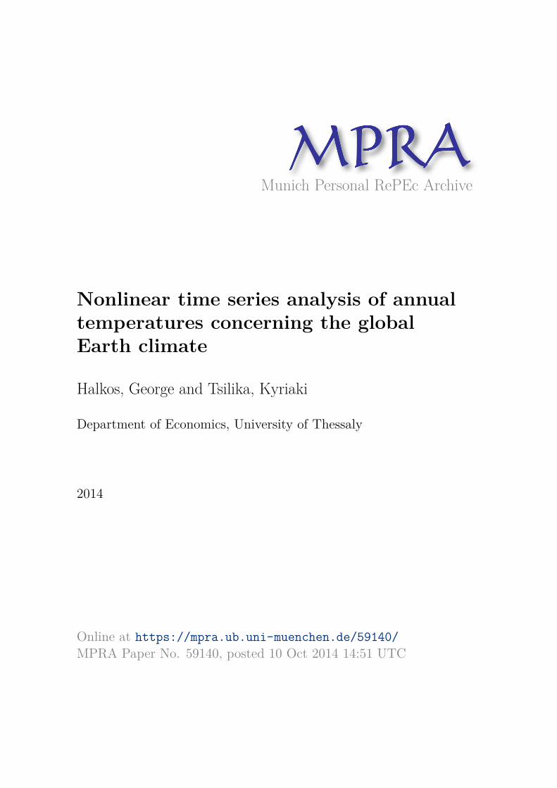
Nonlinear time series analysis of annual

temperatures concerning the global

Earth climate

Halkos, George and Tsilika, Kyriaki

Department of Economics, University of Thessaly

2014

Online at https://mpra.ub.uni-muenchen.de/59140/

MPRA Paper No. 59140, posted 10 Oct 2014 14:51 UTC

1

�

��

��

�

�

��

�� !��"��

#�

1 Laboratory of Operations Research, Department of Economics

University of Thessaly

2 Democritus University of Thrace, Greece,

Department of Electrical and Computer Engineering

�

�

�

��

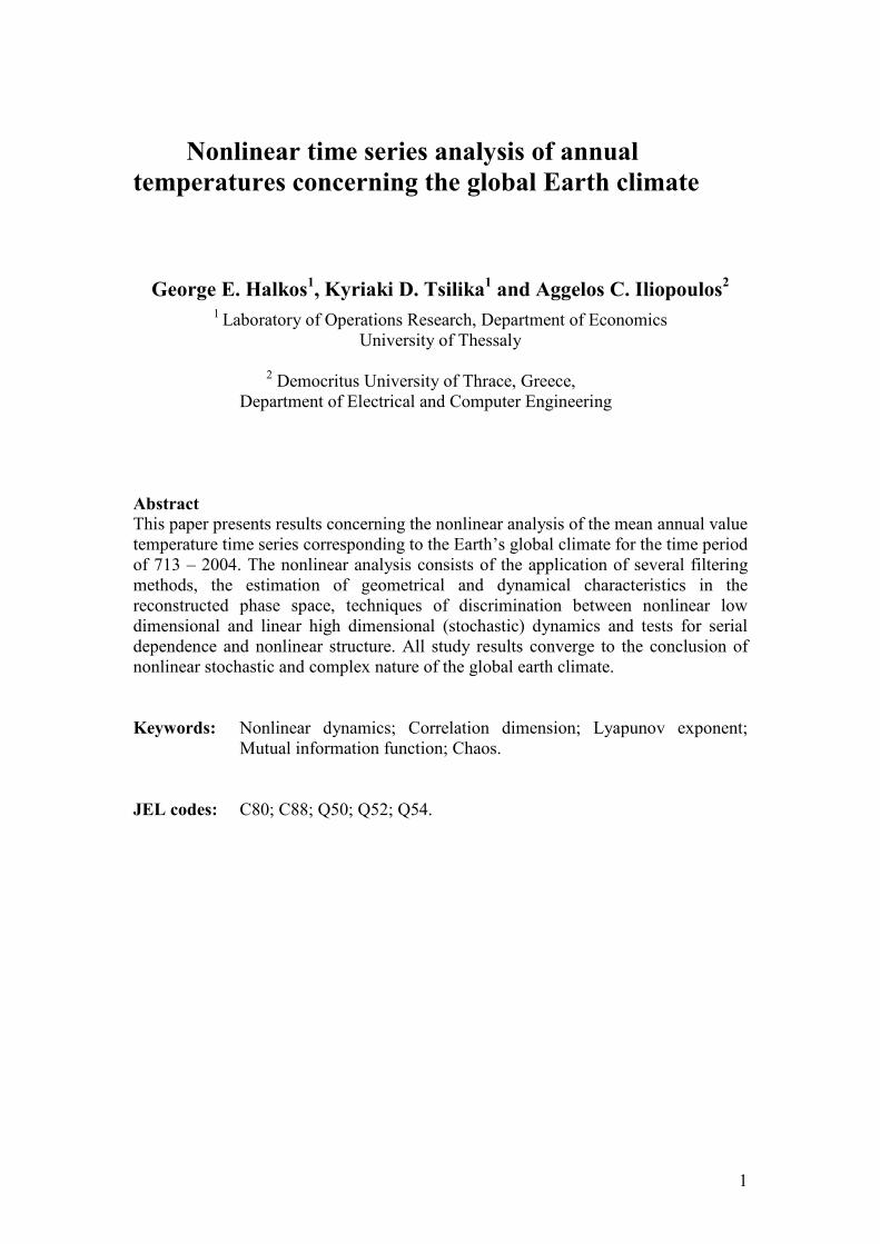
This paper presents results concerning the nonlinear analysis of the mean annual value

temperature time series corresponding to the Earth’s global climate for the time period

of 713 – 2004. The nonlinear analysis consists of the application of several filtering

methods, the estimation of geometrical and dynamical characteristics in the

reconstructed phase space, techniques of discrimination between nonlinear low

dimensional and linear high dimensional (stochastic) dynamics and tests for serial

dependence and nonlinear structure. All study results converge to the conclusion of

nonlinear stochastic and complex nature of the global earth climate.

�

�� $��% Nonlinear dynamics; Correlation dimension; Lyapunov exponent;

Mutual information function; Chaos.

�

&�'��% C80; C88; Q50; Q52; Q54.

�

�

�

�

�

�

�

2

��"��

The climate system of the Earth consists of natural spheres (atmosphere,

biosphere, hydrosphere and geosphere), the humansphere (economy, society, culture)

and their complex interactions (Schellnhuber, 1999; Halkos, 2013). Gedalin &

Balikhin (2008) claim that these interactions as well as the multi;level structure of the

system atmosphere;ocean;solid surface, ocean currents and winds, the differential

absorption volume of solar radiation, the effects of chemical composition, etc lead to

a three dimensional field of the distribution of temperatures presenting much smaller

spatial and temporal scales compared to Earth radius and planet’s rotation period

respectively. At the same time, observations show episodes of abrupt change, starting

with the sudden onset of large global warming (e.g. the end of the last ice age) to the

active and rapid regional changes in hydroclimatic cycle, rainfall and drought (e.g.

desert extension) (Rial et al., 2004).

In addition, there is a wide range of interactions found in the magnitudes of

changes in temperatures that show multifractality (multiple self;similarity) in the

Earth's climate on time scales of 1;100 years (Ashkenazy et al., 2003). These large;

scale changes in temperatures mainly depend on external influences such as physical

effects on air temperature near the Earth's surface, like for instance variations in

volcanic eruptions, the El Niño Southern Oscillation phenomenon, active water cycle

(Nordstrom et al., 2005), solar radiation cycles (Ozawa et al., 2003), changes in the

Earth orbital motion and continents (Lin et al., 1991), while the state change occurs at

a slow time scale.

Moreover, all human actions that affect the state of the climate system such as

changes in the concentration of greenhouse gases and in small gas fractions

controlling the content of stratospheric ozone, sulfur dioxide etc can be considered as

3

small external shocks (Dymnikov & Gritsoun, 2001). All of the above non;linear and

disproportionate inputs;outputs, the created chains of feedback and inner circles,

multiple equilibria, astronomical effects etc create non;linear, stochastic and complex

nature of global climate on Earth.

In this study we present tools as well as methodology of the modern

nonlinear time series analysis used for tracing nonlinear and chaotic dynamics in the

Earth’s climate complex system. The nonlinear algorithm is applied in the annual

temperature time series concerning the Global Earth Climate during the time period

of 713;2004 (D'Arrigo et al. 2006a, b).1 In order to extract useful information about

the complex dynamics of the Earth’s climate we use different filtering methods such

as the AR(4) residuals2 and the SVD analysis. In particular, we estimate geometrical

and dynamical characteristics in the reconstructed phase space such as correlation

dimension, mutual information and maximum Lyapunov exponent.

In addition, BDS test of independence and identical distribution and Brock’s

Residual test are applied to the AR(4) residuals of the Temperature time series,

searching for more evidence of nonlinearity in the data. Finally, the method of

stochastic surrogate data is employed for the exclusion of ‘pseudo;chaos’ caused by

the nonlinear distortion of a purely stochastic process. Our results indicate the

nonlinear stochastic profile of the Earth’s complex climate dynamics.

�

1 The data set is the Northern Hemisphere Tree;Ring;Based STD and RCS Temperature

Reconstructions and the contributors are Rosanne D'Arrigo and Gordon Jacoby, Lamont;Doherty Earth

Observatory, and Rob Wilson, University of Edinburgh.

2 A number of autoregressive schemes to the data set at hand were fitted relying on the statistical

significance of their components and selecting their complexity by the use of the AIC.

4

#��(��)��

This section presents results concerning the nonlinear analysis of the annual

temperature time series. The nonlinear analysis consists of the estimation of

geometrical and dynamical characteristics in the reconstructed phase space and the

techniques of discrimination between nonlinear low dimensional and linear high

dimensional (stochastic) dynamics.4

2.1 Annual temperature time series

In Figure 1a the mean annual value temperature time series is presented

corresponding to the Earth’s global climate for the time period of 713 – 2004. As can

be seen in this figure the time series is stationary apart from the last part where a

significant increase takes place. This increase could be due to the so called

“greenhouse” effect (for more details see Halkos, 2014).

Figure 1b presents the autocorrelation coefficient of the time series estimated

for 100 lags. As can be seen the autocorrelation coefficient decays slowly indicating

the presence of long range correlations of the underlying dynamics. The profile of the

power spectrum, shown in Figure 1c indicates the presence of two distinct dynamics

underlying the temperature time series, one corresponding to a power law scaling as

seen in low frequencies indicating a long range correlation process and another one

corresponding to a flat spectrum indicating an uncorrelated (white noise) process.

Finally, in Figure 1d the slopes of correlation integral estimated for a fixed embedding

dimension m=8 and for three different time reconstruction delays τ=2, 4, 6, is

3 Part of the analysis was presented in the 6

th International Conference from Scientific Computing to

Computational Engineering (6th

IC;SCCE), Athens, Greece, July 11 2014.

4 A complete review concerning the methodology of nonlinear time series analysis and its application

in various geophysical time series can be fount in Athanasiu & Pavlos (2001), Pavlos et al. (2004),

Pavlos et al. (2007), Iliopoulos et al. (2008), Iliopoulos & Pavlos (2010) and references within.

5

presented. As can be observed there is not any saturation, dlnc/dlnr = dm ≠ steady or

scaling of the slopes for ln(r). This result indicates that the underlying dynamics do

not correspond to a low dimensional attractor and is high dimensional (practically

infinite degrees of freedom).

0 400 800 1200 1600

Years

�1.5

�1

�0.5

0

0.5

1

0C

Global Annual Temperature

(a)

1 10 100 1000

Log(f)

0.0001

0.001

0.01

0.1

1

Lo

g P

(f)

Annual Temperature (c)

Figure 1a: Mean annual value temperature time

series Figure 1c: Power spectrum

0 20 40 60 80 100

Lag Time (k)

0

0.2

0.4

0.6

0.8

1

Au

toco

rre

latio

n C

oe

ffic

ien

t (r

k)

(b)Annual Temperature

�3 �2.5 �2 �1.5 �1 �0.5 0

Ln(r)

0

1

2

3

4

5

6

7

8

9

10

Slo

pes

m=8

τ=2

τ=6

τ=4

(d)

Figure 1b: Autocorrelation coefficient

Figure 1d: Slopes of the correlation integrals

as estimated for embedding dimension m=8

and time delay τ=2, 4, 6.

In Figure 2 we present results corresponding to the method of surrogate data.

Usually, this method is used for the rejection of the null hypothesis of the “pseudo;

chaos” existence and the results presented previously exclude the existence of low

dimensional dynamics underlying the temperature time series. However, we can still

use the surrogate data method as an indicator of nonlinearity or even high dimensional

chaos (if the difference between the surrogate data and the original time series is

significant).

6

�3.5 �3 �2.5 �2 �1.5 �1 �0.5 0 0.5

Ln(r)

0

1

2

3

4

5

6

7

8

9

10

SL

OP

ES

m=6,τ=6

Annual Temperature

Surrogates

(e)

�2.5 �2 �1.5 �1 �0.5 0

Ln(r)

0

0.5

1

1.5

2

2.5

Sig

nific

ance

Slopes

Figure 2a: Slopes of the correlation integrals of

the original time series and 10 surrogate data as

estimated for embedding dimension m=6 and

time delay τ=6.

Figure 2d: Significance of the difference of the

statistics between the original time series and 10

surrogate data concerning the slopes of the

correlation integrals.

0 4 8 12 16 20

Lag (τ)

0

0.5

1

1.5

2

2.5

MU

TU

AL

IN

FO

RM

AT

ION

0 4 8 12 16 20

0

0.2

0.4

0.6

0.8

Annual Temperatures

Surrogates

(g)

2 3 4 5 6 7 8 9 10 11 12 13 14 15 16 17 18 19 20

Lag time (τ)

0

1

2

3

4

Sig

nif

ica

nc

eMutual Information

Figure 2b: Mutual Information estimated for the

original time series and 10 surrogate data.

Figure 2e: Significance of the difference of the


surrogate data concerning the mutual

information.

0 100 200 300 400 500 600

Time (Years)

0

0.4

0.8

1.2

1.6

Ma

xim

um

Ly

ap

un

ov

Ex

po

ne

nt

m=6, τ=6(f)

0 200 400 600

Time (Years)

0

0.4

0.8

1.2

1.6

2

Sig

nific

ance

Lmax

Figure 2c: Maximum Lyapunov exponent for

the original time series and 10 surrogate data


time delay τ=6.

Figure 2f: Significance of the difference of the


surrogate data concerning the maximum

Lyapunov exponent.

7

In particular, Figure 2a presents the slopes of the correlation integral estimated

for the original temperature time series and its 10 surrogate data, for embedding

dimension m=6 and time delay τ=6. As can be seen there is no significant difference;

a result depicted also in Figure 2d which presents the significance of the

discrimination of the statistics of Figure 2a, attaining values below 2 for a wide range

of ln(r). This result indicates high dimensional dynamics underlying the original time

series.

In Figure 2b we present the mutual information estimated for the original

temperature time series and for its 10 surrogate data, while in Figure 2e we present the

significance of the statistics. The significance attains values above 2 for the three first

values, however the mutual information value is lower than the corresponding of the

surrogate data, a result that indicates linearity. Finally, Figure 2c presents the

maximum Lyapunov exponent estimated for the original time series and its 10

surrogate data for parameters m=6 and τ= 6, while in Figure 2f the significance of the

statistics is presented. Even though the maximum Lyapunov exponent is positive there

is no difference from the corresponding exponents of the surrogate data. Overall, the

results show that the original time series correspond to high dimensional dynamics.

�

)��*��*��

The present study presents the results of two tests for nonlinear dependence in

annual earth temperatures from 713 up to 2004. The first one is the BDS test of

independence and identical distribution and the second one is Brock’s Residual test.

Similar studies have been carried out in Willey (1992), Frank and Stengos (1988a, b),

Frank et al. (1988), Chavas and Holt (1993). These tests substitute the typical

statistical tests using spectral analysis and autocorrelation function that fail to reveal

8

statistically significant correlations on non;independent data and cannot discriminate

between a stochastic explanation and a deterministically chaotic explanation of a time

series.

The correlation coefficient diagram for the residuals of an AR(4) model fitted

to temperature data in Figure 3a shows statistically insignificant correlations. This

means that the AR(4) model succeeded in removing from the temperature series the

linear structure. The correlation coefficient diagram and the flat profile of the log;log

plot of the power spectrum (Figure 3b) indicate that AR(4) residuals are white noise

residuals.

0 2 4 6 8

Lag Time (k)

�0.2

0

0.2

0.4

0.6

0.8

1

Au

toco

rre

latio

n C

oe

ffic

ien

t

Residuals_AR(4)(b)

1 10 100 100

Log (f)

0.0001

0.001

0.01

0.1

Log P

(f)

RESIDUALS_AR(4)(c)

Figure 3a: Correlation coefficient of AR(4)

residual series

Figure 3b: Power spectrum of AR(4)

residual series

3.1 BDS Test of Independence

Brock, Dechert and Scheinkman (BDS in Brock et al., 1996) created a test for

time based dependence in a series. It is a test of the null hypothesis that the data are

independent and identically distributed (i.i.d. data) against a variety of possible

departures from independence including linear dependence, nonlinear dependence or

chaos. This test can be applied to a series of residuals of estimated linear models in

order to test for extra structure. For example, the residuals from an ARMA model can

be tested to see if there is any nonlinear dependence in the series after the linear

9

ARMA model has been fitted. This way the BDS test of residuals performs a test of a

new hypothesis of an underlying nonlinear process and thus can be employed as a test

for nonlinearity.

��% BDS Test for residuals generated by AR(4) process (e is a multiple of the

standard deviation of the series) e=0.5

Dimension BDS Statistic Std. Error z�Statistic Prob.

2 0.003262 0.000790 4.127598 0.0000

3 0.002793 0.000524 5.326703 0.0000

4 0.001895 0.000261 7.258768 0.0000

5 0.001038 0.000114 9.121463 0.0000

6 0.000503 4.59E�05 10.94192 0.0000

7 0.000197 1.76E�05 11.15649 0.0000

8 6.81E�05 6.52E�06 10.44085 0.0000

e=1


2 0.009244 0.001920 4.814101 0.0000

3 0.014139 0.002353 6.009269 0.0000

4 0.016815 0.002161 7.779901 0.0000

5 0.016582 0.001738 9.540243 0.0000

6 0.014341 0.001294 11.08694 0.0000

7 0.011323 0.000915 12.37596 0.0000

8 0.008427 0.000624 13.50136 0.0000

e=1.5


2 0.010220 0.002044 4.998774 0.0000

3 0.020484 0.003348 6.117933 0.0000

4 0.031566 0.004108 7.684830 0.0000

5 0.041031 0.004410 9.303869 0.0000

6 0.046963 0.004381 10.72055 0.0000

7 0.048953 0.004135 11.84003 0.0000

8 0.047877 0.003763 12.72204 0.0000

e=2


2 0.007245 0.001440 5.029779 0.0000

3 0.016613 0.002746 6.050690 0.0000

4 0.029420 0.003918 7.508800 0.0000

5 0.044021 0.004892 8.997795 0.0000

6 0.057941 0.005651 10.25289 0.0000

7 0.069139 0.006202 11.14861 0.0000

8 0.075744 0.006563 11.54132 0.0000

10

To perform the test, a distance e is chosen. If a pair of points is considered, the

probability of the distance between these points being less or equal to e will be

constant in case the observations of the series are truly i.i.d. In Table 1, probabilities

converge to 0 in all considered embedding dimensions and distances e.

In order to enhance the evidence of nonlinearity, the BDS test is applied to a

series of shuffled residuals (Scheinkman and LeBaron 1989) and to a series of

surrogate residuals (Schreiber and Schmitz 1996). The shuffled residuals is a new

series of the same length as the original AR(4) residual series, created by random

sampling from it with replacement. The surrogate residual series has the same length,

the same autocorrelation function and probability density with the series of AR(4)

residuals. Here, the surrogate residuals are constructed using the improved algorithm

of Schreiber and Schmitz.

3.1.1 BDS Test for shuffled AR(4) residuals

The shuffled AR(4) residuals are used to check the reliability of the BDS test.

According to Scheinkman and LeBaron (1989) we get the original time series and

sampling randomly with replacement from it. The shuffled series will have the same

length as the original. As shuffling destroys the alleged non;linear structure of the

data, the statistical BDS (z;statistic) should detect the difference between the shuffled

and initial time series of AR(4) residuals.

3.1.2 BDS Test for surrogate AR(4) residuals

The surrogate data are random numbers with the same probability density

function and the same autocorrelation function as the original time series. They are

generated using the improved algorithm Schreiber;Schmitz (Schreiber and Schmitz

1996). The BDS statistic should detect in the case of surrogate data as well, the

difference between the surrogate and original AR(4) residual time series.

11

��#% BDS Test for the shuffled series of AR(4) residuals (e is a multiple of the

standard deviation of the series)

e=0.5


2 �2.01E�05 0.000703 �0.028636 0.9772

3 �0.000409 0.000459 �0.891495 0.3727

4 �0.000162 0.000225 �0.720191 0.4714

5 �7.70E�05 9.63E�05 �0.800314 0.4235

6 �4.33E�05 3.82E�05 �1.133358 0.2571

7 �1.47E�05 1.44E�05 �1.022919 0.3063

8 �9.45E�06 5.24E�06 �1.803039 0.0714

e=1


2 �0.000268 0.001790 �0.149962 0.8808

3 �0.000940 0.002174 �0.432576 0.6653

4 �0.000463 0.001979 �0.233736 0.8152

5 �0.000303 0.001577 �0.192206 0.8476

6 6.40E�05 0.001163 0.054976 0.9562

7 0.000222 0.000815 0.272031 0.7856

8 0.000274 0.000551 0.497182 0.6191

e=1.5


2 �0.000902 0.001961 �0.459705 0.6457

3 �0.001740 0.003199 �0.543934 0.5865

4 �0.001142 0.003909 �0.292209 0.7701

5 3.50E�05 0.004180 0.008361 0.9933

6 0.001631 0.004136 0.394342 0.6933

7 0.002416 0.003888 0.621390 0.5343

8 0.003353 0.003525 0.951351 0.3414

e=2


2 �0.001187 0.001392 �0.852656 0.3939

3 �0.001676 0.002655 �0.631513 0.5277

4 �0.001730 0.003790 �0.456534 0.6480

5 �0.000597 0.004733 �0.126043 0.8997

6 0.001837 0.005469 0.335914 0.7369

7 0.003755 0.006004 0.625474 0.5317

8 0.006207 0.006356 0.976601 0.3288

�

�

�

�

12

��)% BDS Test for a randomly selected series of surrogate AR(4) residuals (e is a

multiple of the standard deviation of the series)

e=0.5


2 0.001355 0.000790 1.713933 0.0865

3 0.000931 0.000524 1.775276 0.0759

4 0.000390 0.000261 1.493032 0.1354

5 0.000166 0.000114 1.461026 0.1440

6 6.20E�05 4.59E�05 1.349033 0.1773

7 2.40E�05 1.76E�05 1.363166 0.1728

8 9.89E�06 6.52E�06 1.516046 0.1295

9 3.52E�06 2.35E�06 1.495197 0.1349

10 5.71E�07 8.31E�07 0.687196 0.4920

e=1


2 0.003955 0.001920 2.059653 0.0394

3 0.004974 0.002353 2.114055 0.0345

4 0.004333 0.002161 2.004720 0.0450

5 0.003042 0.001738 1.750358 0.0801

6 0.001844 0.001294 1.425599 0.1540

7 0.001094 0.000915 1.195582 0.2319

8 0.000486 0.000624 0.779270 0.4358

9 0.000162 0.000415 0.391184 0.6957

10 6.36E�05 0.000270 0.235989 0.8134

e=1.5


2 0.005025 0.002044 2.457751 0.0140

3 0.008404 0.003348 2.510072 0.0121

4 0.009652 0.004108 2.349746 0.0188

5 0.008760 0.004410 1.986365 0.0470

6 0.007402 0.004381 1.689747 0.0911

7 0.006157 0.004135 1.489052 0.1365

8 0.004442 0.003763 1.180364 0.2379

9 0.003034 0.003334 0.909864 0.3629

10 0.002102 0.002893 0.726560 0.4675

e=2


2 0.003870 0.001440 2.686398 0.0072

3 0.007293 0.002746 2.656265 0.0079

4 0.009613 0.003918 2.453417 0.0142

5 0.009802 0.004892 2.003532 0.0451

6 0.009653 0.005651 1.708092 0.0876

7 0.009292 0.006202 1.498362 0.1340

8 0.007954 0.006563 1.211922 0.2255

9 0.006512 0.006759 0.963461 0.3353

10 0.005344 0.006817 0.783967 0.4331

13

The results clearly show that in both series of shuffled and surrogate AR(4)

residuals the null hypothesis for i.i.d data cannot be rejected since z statistic takes

statistically insignificant values in the vast majority of embedding dimensions and e.

The BDS statistic (z;statistic in Table 4) is expected to diagnose the difference

between the original AR(4) residuals and the shuffled and surrogate residuals, given

that their generating process destroys the (possible) nonlinear structure of the original

residuals. If the residuals are i.i.d. data then the BDS test statistic is normally

distributed [z;statistic∼N(0,1)].

The values of z;statistic for AR(4) residuals exceed the critical value for every

significant level, in all embedding dimensions and distances e. The conclusion is to

reject the null hypothesis of independence of AR(4) residuals (Halkos, 2006). This is

an indication that the series is generated by a nonlinear process, given that all the

linear structure has been removed. The results also show that in both series of shuffled

and surrogate residuals the i.i.d. null hypothesis is retained, since z;statistic values are

less than critical values in the vast majority of embedding dimensions and distances e.

Aiming to check the reliability of BDS statistic in our data, we apply the

following methodology:

*��: We generate 30 surrogate residual series using the Schreiber and Schmitz

algorithm,

*��#: We perform BDS test in each one of them and

*��): We compute mean value surro� and standard deviation surroσ of the

distribution of the z;statistics of step 2.

�

14

��+% BDS statistics for annual earth temperature data, AR(4) residuals, shuffled

and surrogate AR(4) residuals (e is a multiple of the standard deviation of the series) ��

��,-��,- (.+/��,-��,-��

�� (.+/�� (.+/��

��

2 0.5 45.24913 4.127598 �0.028636 �2.217687

3 0.5 57.37534 5.326703 �0.891495 �1.074243

4 0.5 72.22246 7.258768 �0.720191 �0.547121

5 0.5 93.62769 9.121463 �0.800314 0.314762

6 0.5 126.4490 10.94192 �1.133358 0.692186

7 0.5 177.9179 11.15649 �1.022919 0.841111

8 0.5 261.0943 10.44085 �1.803039 0.177648

2 1 39.84653 4.814101 �0.149962 �2.346665

3 1 45.91428 6.009269 �0.432576 �1.248528

4 1 50.96965 7.779901 �0.233736 �0.298179

5 1 57.74778 9.540243 �0.192206 0.094204

6 1 66.57659 11.08694 0.054976 0.138372

7 1 78.26005 12.37596 0.272031 0.209266

8 1 94.22354 13.50136 0.497182 0.233027

2 1.5 36.70460 4.998774 �0.459705 �2.372047

3 1.5 39.50391 6.117933 �0.543934 �1.424346

4 1.5 40.56742 7.684830 �0.292209 �0.455554

5 1.5 41.99484 9.303869 0.008361 �0.047905

6 1.5 43.73042 10.72055 0.394342 0.007883

7 1.5 45.99300 11.84003 0.621390 0.188030

8 1.5 48.80326 12.72204 0.951351 0.271578

2 2 34.58071 5.029779 �0.852656 �2.236987

3 2 35.68591 6.050690 �0.631513 �1.233640

4 2 35.05630 7.508800 �0.456534 �0.279808

5 2 34.70645 8.997795 �0.126043 0.098948

6 2 34.47040 10.25289 0.335914 0.267017

7 2 34.41821 11.14861 0.625474 0.544960

8 2 34.52596 11.54132 0.976601 0.659747 ��

In Table 5 the difference between the BDS statistic of 30 surrogate residual

series and the original residual series is evaluated, computing significance

surro

surrooriginalS

σ

�� −= , a quantity without units of measure (Papaioannou, 2000).

original� is the z;statistic of the original AR(4) residuals. When the value of

significance S is higher than 2;3, then, the probability that the original AR(4)

15

residuals does not belong in the same family of the surrogate data is higher than 0.95;

0.99.

��0%�Evaluation of the Significance S

��1��,-��,- (.+/��,-��*�

2 0.5 0.046493 4.1276 1.20897689 3.3756704

3 0.5 �0.00535 5.3267 1.04810525 5.0873204

4 0.5 �0.01428 7.2588 1.04883585 6.93442741

5 0.5 0.024699 9.1215 1.06811817 8.51666211

6 0.5 0.123513 10.9419 1.13927845 9.49582332

7 0.5 0.231672 11.1565 1.3338781 8.19027475

8 0.5 0.283587 10.4409 1.65918973 6.12185161

�

2 1 0.079205 4.8141 1.12199284 4.22007595

3 1 0.075377 6.0093 0.96038479 6.17869293

4 1 0.066815 7.7799 0.98676735 7.81651824

5 1 0.068257 9.5402 0.96808426 9.78421362

6 1 0.142875 11.0869 0.98222931 11.1420262

7 1 0.164796 12.376 1.0405768 11.7350334

8 1 0.126813 13.5014 1.08324927 12.3467311

�

2 1.5 0.110494 4.9988 1.16931166 4.18049912

3 1.5 0.105937 6.1179 0.99625702 6.03455028

4 1.5 0.096003 7.6848 0.99167558 7.65250008

5 1.5 0.071912 9.3039 0.98810418 9.34313228

6 1.5 0.126033 10.7206 0.98864506 10.7162498

7 1.5 0.164304 11.84 1.03462214 11.2849856

8 1.5 0.171682 12.722 1.0558221 11.886773

�

2 2 0.122381 5.0298 1.21619584 4.0350567

3 2 0.115367 6.0507 1.02923922 5.76671855

4 2 0.101784 7.5088 0.98702881 7.50435657

5 2 0.056389 8.9978 0.99608486 8.97655523

6 2 0.088089 10.2529 0.98540762 10.3153365

7 2 0.105492 11.1486 1.04405218 10.577161

8 2 0.127608 11.5413 1.06849091 10.6820679

S values presented in Table 5 are considerably high, meaning that the BDS statistic

results differently for surrogate and original data. This is another evidence to reject

the hypothesis that AR(4) residuals are linearly dependent noisy data.

3.2 Brock’s Residual Test

Brock (1986) has proposed a test based on the invariance to linear

transformations (like an AR process) that holds for chaotic data: if one transforms

16

chaotic data linearly, both the original and the transformed data may have the same

correlation dimension and Lyapunov exponents.

The process followed here (proposed by Brock and Sayers, 1988) permits a

nonlinear test for the existence of a deterministic system and the refusal of a linear

generating process if accepted. The dimension and the maximum Lyapunov exponent

of the residuals is estimated and compared with the dimension and the maximum

Lyapunov exponent of the original data. If any nonlinear structure exists, these values

will be untouched.

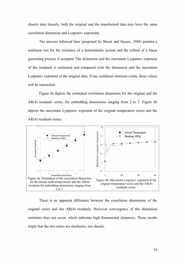
Figure 4a depicts the estimated correlation dimension for the original and the

AR(4) residuals series, for embedding dimensions ranging from 2 to 7. Figure 4b

depicts the maximum Lyapunov exponent of the original temperature series and the

AR(4) residuals series.

2 3 4 5 6 7

Embedding Dimension

0

2

4

6

8

Corr

ela

tio

n D

ime

nsio

n

Annual Temperature

Residual_AR(4)

0 200 400 600

�0.4

0

0.4

0.8

1.2

1.6

Ma

xim

um

Ly

ap

un

ov

Ex

po

ne

nt

Annual Temperature

Residual_AR(4)

Figure 4a: Estimation of the correlation dimension

for the annual earth temperatures and the AR(4)

residuals for embedding dimensions ranging from

2 to 7.

Figure 4b: Maximum Lyapunov exponent of the

original temperature series and the AR(4)

residuals series.

There is no apparent difference between the correlation dimensions of the

original series and the AR(4) residuals. However convergence of the dimension

estimates does not occur, which indicates high dimensional dynamics. These results

imply that the two series are stochastic, not chaotic.

17

Caution is required in the interpretation of this diagnostic. A bias has been

shown in the case of relatively small data sets (100 to 2000 observations) as the series

studied here of 1292 observations. This bias corresponds to estimation errors in the

dimension estimates leading to rejection of deterministic chaos even if it exists (Brock

1988; Hsieh 1989; Ramsey at al. 1990).

�

+�� (.+/�(��

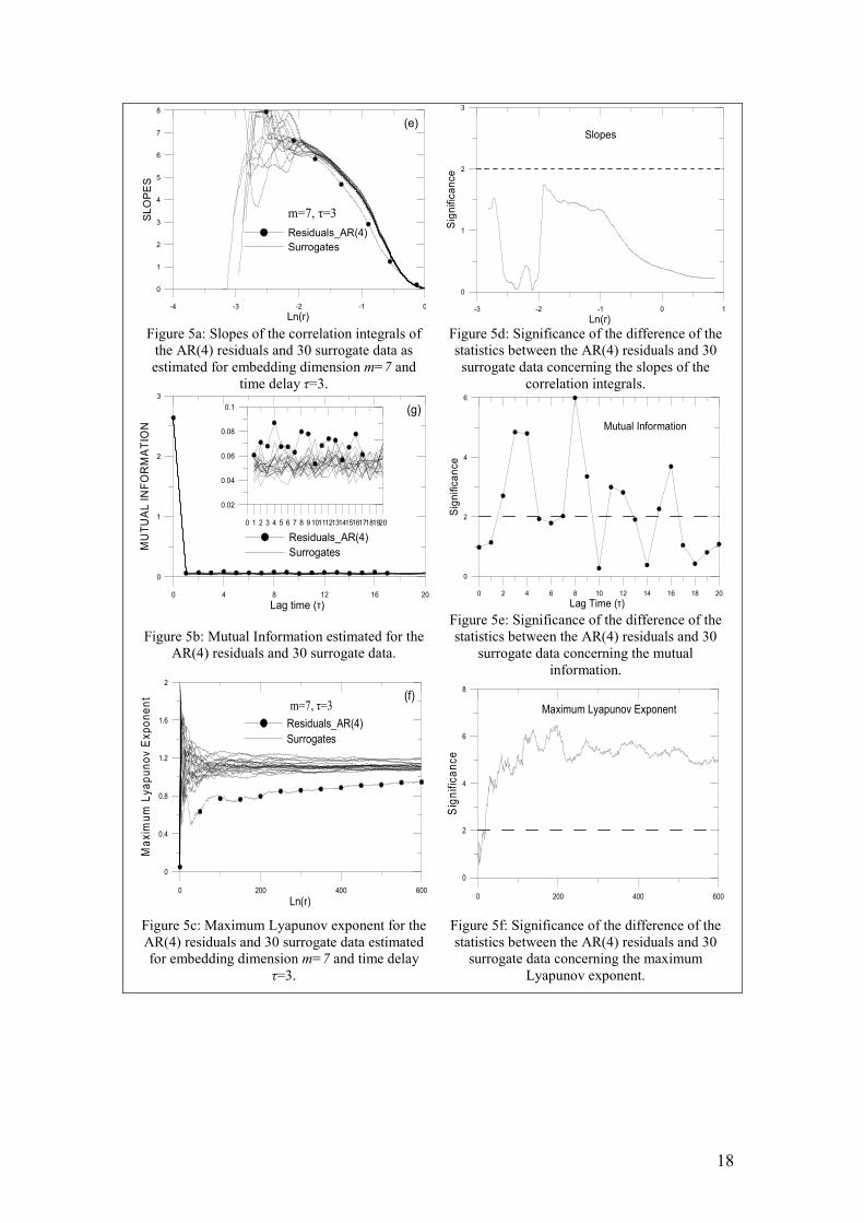
In Figure 5 we present results concerning the method of surrogate data. In

particular, in Figure 5a the slopes of correlation integral estimated for the AR(4)

residuals time series and 30 surrogate data are shown. For the estimation we used

embedding dimension m=7 and time delay τ =3. As it can be observed there is no

difference, a result clearly depicted in Figure 5d which shows the significance of

discrimination statistics between the AR(4) time series and its surrogates.

The value of significance is S < 2 for all Ln(r). This result reveals the high

dimensional character of the underlying dynamics corresponding to the residuals. In

addition, in Figure 5b we present the comparison of the mutual information of the

AR(4) time series and its surrogates, while in Figure 5e the significance of the

discriminating statistics is shown. The significance attains large values above 2 for

some τ, indicating long range nonlinear interactions.

Finally in Figures 5(c, f) the difference between the AR(4) time series and its

surrogate data is obvious and significant, a result indicating that the AR(4) time series

is more deterministic and less stochastic, since the Lmax of the AR(4) is much

smaller from the corresponding of surrogates. Thus, the filtering used in order to

generate the AR(4) residuals, revealed a hidden nonlinear dynamics of lesser

complexity, in contrast to the analysis of the original annual temperature.

18

�4 �3 �2 �1 0

Ln(r)

0

1

2

3

4

5

6

7

8

SL

OP

ES

Residuals_AR(4)

Surrogates

m=7, τ=3

(e)

�3 �2 �1 0 1

Ln(r)

0

1

2

3

Sig

nific

an

ce

Slopes

Figure 5a: Slopes of the correlation integrals of

the AR(4) residuals and 30 surrogate data as


time delay τ=3.


statistics between the AR(4) residuals and 30



0 4 8 12 16 20

Lag time (τ)

0

1

2

3

MU

TU

AL

IN

FO

RM

AT

ION

Residuals_AR(4)

Surrogates

0 1 2 3 4 5 6 7 8 9 1011121314151617181920

0.02

0.04

0.06

0.08

0.1 (g)

0 2 4 6 8 10 12 14 16 18 20

Lag Time (τ)

0

2

4

6

Sig

nific

an

ce

Mutual Information

Figure 5b: Mutual Information estimated for the

AR(4) residuals and 30 surrogate data.



surrogate data concerning the mutual

information.

0 200 400 600

Ln(r)

0

0.4

0.8

1.2

1.6

2

Ma

xim

um

Ly

ap

un

ov

Ex

po

ne

nt

Residuals_AR(4)

Surrogates

m=7, τ=3(f)

0 200 400 600

0

2

4

6

8

Sig

nif

ica

nc

e

Maximum Lyapunov Exponent

Figure 5c: Maximum Lyapunov exponent for the

AR(4) residuals and 30 surrogate data estimated

for embedding dimension m=7 and time delay

τ=3.



surrogate data concerning the maximum

Lyapunov exponent.

�

�

�

19

0�� *2��!��

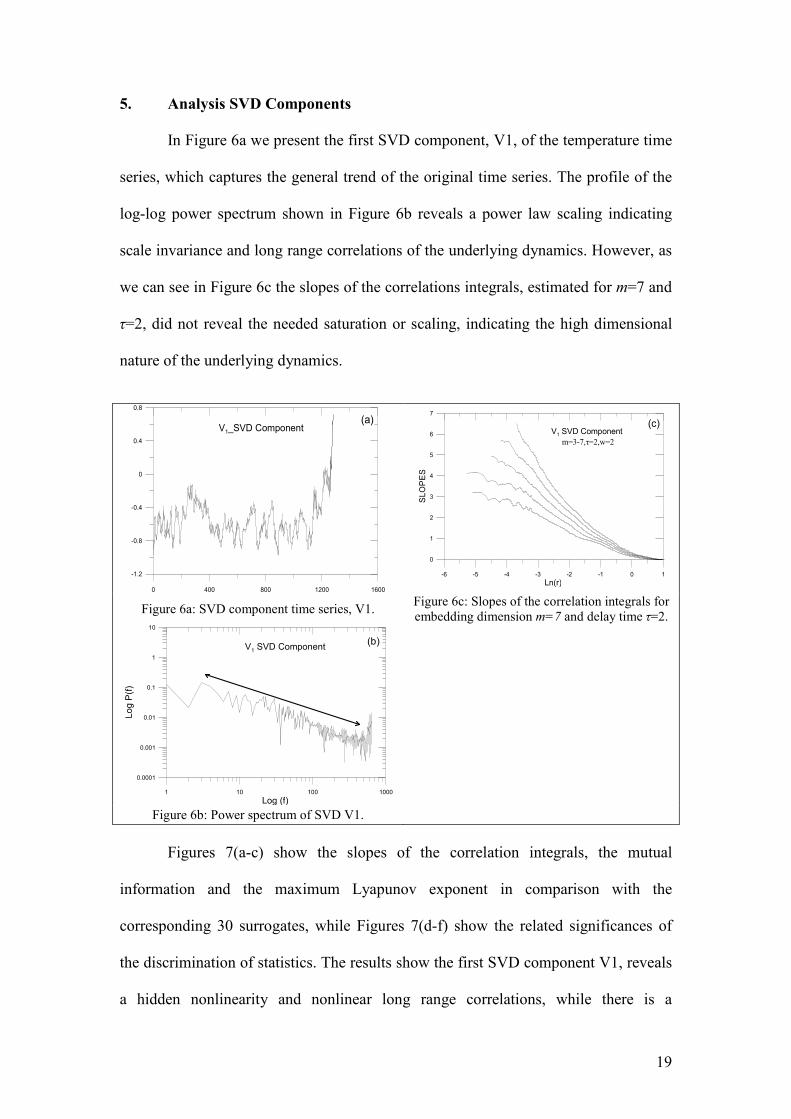
In Figure 6a we present the first SVD component, V1, of the temperature time

series, which captures the general trend of the original time series. The profile of the

log;log power spectrum shown in Figure 6b reveals a power law scaling indicating

scale invariance and long range correlations of the underlying dynamics. However, as

we can see in Figure 6c the slopes of the correlations integrals, estimated for m=7 and

τ=2, did not reveal the needed saturation or scaling, indicating the high dimensional

nature of the underlying dynamics.

0 400 800 1200 1600

�1.2

�0.8

�0.4

0

0.4

0.8

V1_SVD Component(a)

�6 �5 �4 �3 �2 �1 0 1

Ln(r)

0

1

2

3

4

5

6

7

SL

OP

ES

V1 SVD Component

m=3;7,τ=2,w=2

(c)

Figure 6a: SVD component time series, V1. Figure 6c: Slopes of the correlation integrals for

embedding dimension m=7 and delay time τ=2.

1 10 100 1000

Log (f)

0.0001

0.001

0.01

0.1

1

10

Lo

g P

(f)

V1 SVD Component(b)

Figure 6b: Power spectrum of SVD V1.

Figures 7(a;c) show the slopes of the correlation integrals, the mutual

information and the maximum Lyapunov exponent in comparison with the

corresponding 30 surrogates, while Figures 7(d;f) show the related significances of

the discrimination of statistics. The results show the first SVD component V1, reveals

a hidden nonlinearity and nonlinear long range correlations, while there is a

20

significant difference of low dimensionality for radius ln(r) = ;3 till ;2. These results

are in agreement and further strengthen the results of the nonlinear analysis

concerning AR(4) residuals.

�4 �3 �2 �1 0 1

Ln(r)

0

1

2

3

4

5

6

7

8

SL

OP

ES

V1 SVD Component

Surrogates

m=7, τ=2, w=2(d)

�4 �3 �2 �1 0 1 2

Ln(r)

0

2

4

6

Sig

nific

ance

Slopes

Figure 7a: Slopes of the correlation integrals

of the SVD V1 component and 20 surrogate

data as estimated for embedding dimension

m=7 and time delay τ=2.


statistics between the SVD V1 component and 20



0 2 4 6 8 10

Lag Time (τ)

0

0.5

1

1.5

2

2.5

Mu

tua

l In

form

atio

n

V1 SVD COMPONENT

(e)

0 2 4 6 8 10

0.4

0.8

1.2

1.6

0 1 2 3 4 5 6 7 8 9 10 11 12 13 14 15 16 17 18 19 20

Lag Time (τ)

0

1

2

3

4

5

Sig

nific

an

ce

Mutual Information

Figure 7b: Mutual Information estimated for

the SVD V1 component and 20 surrogate

data.



surrogate data concerning the mutual information.

0 200 400 600 800 1000

�0.1

0

0.1

0.2

0.3

Ma

xim

um

Lya

pu

no

v E

xp

on

en

t

V1 SVD Component

m=8,τ=1

(f)

0 200 400 600

0

1

2

3

4

Sig

nific

ance

Lmax

Figure 7c: Maximum Lyapunov exponent for

the SVD V1 component and 20 surrogate data


time delay τ=1.



surrogate data concerning the maximum Lyapunov

exponent

21

The next SVD components (Figures. 8(a;d)) capture the noise component that

affects the original data. As it can be seen in these Figures the V2 SVD component

corresponds to a high dimensional and linear dynamic process. In particular, the

power spectrum has a flat profile (Figure 8b), the mutual information of the V2 SVD

component cannot be discriminated from its surrogates (Figure 8d) and the slopes of

the correlation integral do not reveal a saturation or a scaling profile (Figure 8c).

0 400 800 1200 1600

�0.4

�0.2

0

0.2

0.4

V2 SVD Component(a)

�6 �4 �2 0

Ln(r)

0

1

2

3

4

5

6

7

8

SL

OP

ES

V2 SVD Component

m=3;8, τ=1

(c)

Figure 8a: SVD component time series, V2. Figure 8c: Slopes of the correlation integrals

for embedding dimension m=8 and delay time

τ=1.

1 10 100

Log (f)

0.0001

0.001

0.01

0.1

Lo

g P

(f)

V2 SVD Component (b)

0 2 4 6 8 10

Lag Time (τ)

0

1

2

3

Mu

tua

l In

form

ati

on

V2 SVD COMPONENT

0 2 4 6 8 10

0

0.1

0.2

0.3

0.4

0.5

(d)

�

Figure 8b: Power spectrum of SVD V2. Figure 8d: Mutual Information estimated for

the SVD V2 component and 20 surrogate data.

The analysis of the next SVD component, V2, which corresponds to the rapid

fluctuations of the original signal, revealed the high dimensionality and the linearity

of the component, properties reminiscent of white noise.

22

3��!��

In the analysis performed, an AR(4) model was fitted to temperature data to

remove the linear structure and the AR(4) residual series was tested using tools and

methodology of the modern nonlinear time series. After applying the BDS test of

independence and identical distribution in AR(4) residuals, the null hypothesis of

independent and identically distributed data was rejected and the underlying nonlinear

data structure was revealed. In addition, Brock’s Residual test results for both the

original and the AR(4) residual series led to the rejection of a linear generating

process for temperatures.

Next, geometrical and dynamical characteristics in the reconstructed phase

space such as correlation dimension, mutual information and maximum Lyapunov

exponent were estimated for the temperature data and the AR(4) residuals. In order to

prove the difference between the (potential) nonlinear process and a nonlinear

distortion of a purely stochastic process, we generated 30 series of surrogate data,

with discriminating statistics the BDS statistic, the maximum Lyapunov exponent and

the mutual information. The nonlinear algorithm for computing geometrical and

dynamical characteristics of the climate system was used once again, after filtering

original temperature data with SVD Analysis. The comparison with stochastic

surrogate data analysis provided more evidence for nonlinearity.

The results indicated the nonlinear stochastic profile of the Earth’s complex

climate dynamics, finding no evidence of deterministic chaos.�Analysis of the (original)

temperature time series revealed a linear stochastic component (white noise), being

dominant in climate dynamics. Applying nonlinear techniques in whitened series gave

strong evidence of nonlinearity and resulted in an underlying dynamics with many

degrees of freedom. This conclusion is in accordance with the widely accepted opinion

that earth’s climate is highly nonlinear and stochastic.

23

(��

�

Ashkenazy Y., Baker D.R., Gildor H. and Havlin S. (2003). Nonlinearity and

Multifractality of climate change in the past 420,000 years, Geophysical

Research Letters )4�(22), 2146.

Athanasiu M.A. and Pavlos G.P. (2001). SVD analysis of the Magnetospheric AE

index time series and comparison with low dimensional chaotic dynamics,

Nonlinear Processes in Geophysics 5, 95;125.

Brock W.A. (1986). Distinguishing Random and Deterministic Systems: abridged

version, Journal of Economic Theory, +4, 168;195.

Brock W.A. (1988). Nonlinearity and Complex Dynamics in Economics and Finance.

In: P. Anderson, K. Arrow and D. Pines (Eds), The Economy as an Evolving

Complex System. New York: Addison Wesley, p. 77;97.

Brock W. and Sayers C. (1988). Is the Business Cycle Characterized by Deterministic

Chaos? Journal of Monetary Economics, ##, 71;90.

Brock W.A., Scheinkman J.A., Dechert W.D. and LeBaron B. (1996). A Test for

Independence Based On the Correlation Dimension, Econometric Reviews �0

(3), 197;235.

Chavas J.P. and Holt M. (1993). On Nonlinear Dynamics: The Case of the Pork

Cycle, American Journal of Agricultural Economics 6), 819;828.

D'Arrigo R., Jacoby G., et al. (2006a). Northern Hemisphere Tree;Ring;Based STD

and RCS Temperature Reconstructions. IGBP PAGES/World Data Center for

Paleoclimatology Data Contribution Series #2006;092. NOAA/NCDC

Paleoclimatology Program, Boulder CO, USA.

D'Arrigo R., Wilson R. and Jacoby G. (2006b). On the long;term context for late

twentieth century warming. Journal of Geophysical Research, ��, D03103,

doi:10.1029/2005JD006352

Dymnikov V.P. and Gritsoun A.S. (2001). Climate model attractors: chaos, quasi;

regularity and sensitivity to small perturbations of external forcing, Nonlinear

Processes in Geophysics �0, 201;209.

Frank M., Gencay R. and Stengos T. (1988). International Chaos? European

Economic Review, )#, 1569;1584.

Frank M. and Stengos T. (1988a). Some Evidence Concerning Macroeconomic

Chaos, Journal of Monetary Economics, ##, 423;438.

Frank M. and Stengos T. (1988b). Chaotic Dynamics in Economic Time series,

Journal of Economic Surveys, # (2), 103;133.

24

Gedalin M. and Balikhin M. (2008). Climate of Utopia, Nonlinear Processes in

Geophysics �0, 541;549.

Halkos G.E. (2006). Econometrics. Theory and Practice, Giourdas Publications,

Athens (in Greek).

Halkos G.E. (2013). Economy and the Environment: Valuation methods and

Management. Liberal Books Publications, Athens (in Greek).

Halkos G.E. (2014). The Economics of Climate Change Policy: Critical review and

future policy directions," MPRA Paper 56841, University Library of Munich,

Germany.

Hsieh D. (1989). Testing for Nonlinear Dependence in Daily Foreign Exchange Rates,

Journal of Business, 3#, 339;368.

Iliopoulos A.C., Pavlos G.P. and Athanasiu M.A. (2008). Spatiotemporal Chaos into

the Hellenic Seismogenesis: Evidence for a Global Strange Attractor,

Nonlinear Phenomena in Complex Systems, �� (2), 274;279.

Iliopoulos A.C. and Pavlos G.P. (2010). Global Low Dimensional Chaos in the

Hellenic Region, International Journal of Bifurcation and Chaos, #4 (7), 2071;

2095.

Lin R.Q., Kreiss H., Kuang W.J. and Leung L.Y. (1991). A study of long;term

climate change in a simple seasonal nonlinear climate model, Climate

Dynamics, 3, S. 35;41.

Nordstrom K.M., Gupta V.K. and Chase T.N. (2005). Role of the hydrological cycle

in regulating the planetary climate system of a simple nonlinear dynamical

model, Nonlinear Processes in Geophysics, �#, 741–753.

Ozawa H., Ohmura A., Lorenz R.D. and Pujol T. (2003). The Second Law of

Thermodynamics and the Global Climate System: A review of the maximum

entropy production principle, Reviews of Geophysics +� (4), 1018.

Papaioannou G. (2000). Chaotic Time Series Analysis: Theory and Practice, Leader

Books, Athens (in Greek).

Pavlos G.P., Athanasiu M.A., Anagnostopoulos G.C., Rigas A.G. and Sarris E.T.

(2004). Evidence for chaotic dynamics in the Jovian magnetosphere, Planetary

and Space Science, 0# (5;6), 513;541.

Pavlos G.P., Iliopoulos A.C. and Athanasiu M.A. (2007). Self Organized Criticality

or / and Low Dimensional Chaos in Earthquake Processes. Theory and Practice

in Hellenic Region, in Nonlinear Dynamics in Geosciences, eds. Tsonis A. &

Elsner J., Springer, 235;259.

25

Ramsey J., Sayers C. and Rothman P. (1990). The Statistical Properties of Dimension

Calculations Using Small Data Sets: Some economic Applications, International

Economic Review, )� (4), 991;1020.

Rial J.A., Pielke Sr. R.A., Beniston M., Claussen M., Canadell J., Cox P., Held H., de

Noblet;Ducoudré N., Prinn R., Reynolds J.F. and Salas J.D. (2004).

Nonlinearities, feedbacks and critical thresholds within the Earth’s climate

system. Climatic Change, 30, 11;38.

Scheinkman J. and B. LeBaron (1989). Nonlinear Dynamics and Stock Returns,

Journal of Business, 3#, 311;337.

Schellnhuber H. J. (1999). Earth System Analysis and the Second Copernican

Revolution, Nature +4#, C19;C26.

Schreiber T. and Schmitz A. (1996). Improved surrogate data for nonlinearity test,

Physical Review Letters, 66, 635;638.

Willey T. (1992). Testing for Nonlinear Dependence in Daily Stock Indices, Journal

of Economic Business, ++, 63;76.

nonlinear time series analysis of annual temperatures ... · nonlinear time series analysis used...

Documents