SANDIA REPORTSAND2007-3257Unlimited ReleasePrinted May 2007

Nonlinearly-Constrained OptimizationUsing Asynchronous ParallelGenerating Set Search

Joshua D. Griffin and Tamara G. Kolda

Prepared bySandia National LaboratoriesAlbuquerque, New Mexico 87185 and Livermore, California 94550

Sandia is a multiprogram laboratory operated by Sandia Corporation,a Lockheed Martin Company, for the United States Department of Energy’sNational Nuclear Security Administration under Contract DE-AC04-94-AL85000.

Approved for public release; further dissemination unlimited.

Issued by Sandia National Laboratories, operated for the United States Department of Energy by SandiaCorporation.

NOTICE: This report was prepared as an account of work sponsored by an agency of the United StatesGovernment. Neither the United States Government, nor any agency thereof, nor any of their employees,nor any of their contractors, subcontractors, or their employees, make any warranty, express or implied,or assume any legal liability or responsibility for the accuracy, completeness, or usefulness of any infor-mation, apparatus, product, or process disclosed, or represent that its use would not infringe privatelyowned rights. Reference herein to any specific commercial product, process, or service by trade name,trademark, manufacturer, or otherwise, does not necessarily constitute or imply its endorsement, recom-mendation, or favoring by the United States Government, any agency thereof, or any of their contractorsor subcontractors. The views and opinions expressed herein do not necessarily state or reflect those ofthe United States Government, any agency thereof, or any of their contractors.

Printed in the United States of America. This report has been reproduced directly from the best availablecopy.

Available to DOE and DOE contractors fromU.S. Department of EnergyOffice of Scientific and Technical InformationP.O. Box 62Oak Ridge, TN 37831

Telephone: (865) 576-8401Facsimile: (865) 576-5728E-Mail: reports@adonis.osti.govOnline ordering: http://www.osti.gov/bridge

Available to the public fromU.S. Department of CommerceNational Technical Information Service5285 Port Royal RdSpringfield, VA 22161

Telephone: (800) 553-6847Facsimile: (703) 605-6900E-Mail: orders@ntis.fedworld.govOnline ordering: http://www.ntis.gov/help/ordermethods.asp?loc=7-4-0#online

DE

PA

RT

MENT OF EN

ER

GY

• • UN

IT

ED

STATES OFA

M

ER

IC

A

2

SAND2007-3257Unlimited ReleasePrinted May 2007

Nonlinearly-Constrained Optimization Using

Asynchronous Parallel Generating Set Search

Joshua D. Griffin and Tamara G. KoldaMathematics, Informatics, and Decision Sciences Department

Sandia National LaboratoriesLivermore, CA 94551-9159jgriffi,tgkolda@sandia.gov

Abstract

Many optimization problems in computational science and engineering (CS&E) are char-acterized by expensive objective and/or constraint function evaluations paired with a lack ofderivative information. Direct search methods such as generating set search (GSS) are well un-derstood and efficient for derivative-free optimization of unconstrained and linearly-constrainedproblems. This paper addresses the more difficult problem of general nonlinear programmingwhere derivatives for objective or constraint functions are unavailable, which is the case for manyCS&E applications. We focus on penalty methods that use GSS to solve the linearly-constrainedproblems, comparing different penalty functions. A classical choice for penalizing constraint vi-olations is `22, the squared `2 norm, which has advantages for derivative-based optimizationmethods. In our numerical tests, however, we show that exact penalty functions based on the`1, `2, and `∞ norms converge to good approximate solutions more quickly and thus are attrac-tive alternatives. Unfortunately, exact penalty functions are discontinuous and consequentlyintroduce theoretical problems that degrade the final solution accuracy, so we also considersmoothed variants. Smoothed-exact penalty functions are theoretically attractive because theyretain the differentiability of the original problem. Numerically, they are a compromise betweenexact and `22, i.e., they converge to a good solution somewhat quickly without sacrificing muchsolution accuracy. Moreover, the smoothing is parameterized and can potentially be adjusted tobalance the two considerations. Since many CS&E optimization problems are characterized byexpensive function evaluations, reducing the number of function evaluations is paramount, andthe results of this paper show that exact and smoothed-exact penalty functions are well-suitedto this task.

3

Contents

1 Introduction . . . . . . . . . . . . . . . . . . . . . . . . . . . . . . . . . . . . . . . . . . . . . . . . . . . . . . . . . . . . . . . . . . . . . . . . . . . . . 52 Algorithmic framework. . . . . . . . . . . . . . . . . . . . . . . . . . . . . . . . . . . . . . . . . . . . . . . . . . . . . . . . . . . . . . . . . . . 93 Exact penalty functions . . . . . . . . . . . . . . . . . . . . . . . . . . . . . . . . . . . . . . . . . . . . . . . . . . . . . . . . . . . . . . . . . . 114 Smoothed exact penalty functions . . . . . . . . . . . . . . . . . . . . . . . . . . . . . . . . . . . . . . . . . . . . . . . . . . . . . . . . 155 Theoretical underpinnings. . . . . . . . . . . . . . . . . . . . . . . . . . . . . . . . . . . . . . . . . . . . . . . . . . . . . . . . . . . . . . . . 196 Related Work . . . . . . . . . . . . . . . . . . . . . . . . . . . . . . . . . . . . . . . . . . . . . . . . . . . . . . . . . . . . . . . . . . . . . . . . . . . . 217 Conclusions . . . . . . . . . . . . . . . . . . . . . . . . . . . . . . . . . . . . . . . . . . . . . . . . . . . . . . . . . . . . . . . . . . . . . . . . . . . . . . 23

Appendix

A Detailed numerical results . . . . . . . . . . . . . . . . . . . . . . . . . . . . . . . . . . . . . . . . . . . . . . . . . . . . . . . . . . . . . . . . 25References. . . . . . . . . . . . . . . . . . . . . . . . . . . . . . . . . . . . . . . . . . . . . . . . . . . . . . . . . . . . . . . . . . . . . . . . . . . . . . . . . . . 29

Figures

1 Contours of various penalty function for two constraints. . . . . . . . . . . . . . . . . . . . . . . . 122 Number of problems that successfully exited for exact methods and `22. . . . . . . . . . . . . 133 Relative difference in final objective value compared to `22. . . . . . . . . . . . . . . . . . . . . . . 144 Number of problems that successfully exited for exact, smoothed-exact, and `22. . . . . . 165 Relative difference in final objective value compared to `22. . . . . . . . . . . . . . . . . . . . . . . 17

Tables

1 Number of problems solved for each penalty function. . . . . . . . . . . . . . . . . . . . . . . . . . . 122 Percentage of the 98 problems solved by all methods that have a relative difference

with `22 no smaller than the specified value. . . . . . . . . . . . . . . . . . . . . . . . . . . . . . . . . . . . 133 Number of problems solved for each penalty function. . . . . . . . . . . . . . . . . . . . . . . . . . . 174 Percentage of the 98 problems solved by all methods that have a relative difference

with `22 no smaller than the specified value. . . . . . . . . . . . . . . . . . . . . . . . . . . . . . . . . . . . 17A.1 Detailed numerical results . . . . . . . . . . . . . . . . . . . . . . . . . . . . . . . . . . . . . . . . . . . . . . . . . 27A.2 Detailed numerical results . . . . . . . . . . . . . . . . . . . . . . . . . . . . . . . . . . . . . . . . . . . . . . . . . 28

Algorithms

1 Generic penalty method . . . . . . . . . . . . . . . . . . . . . . . . . . . . . . . . . . . . . . . . . . . . . . . . . . 9

4

1 Introduction

In computational science and engineering (CS&E), optimization problems do not always match thetextbook. As a motivating application, consider the typical problem of parameter tuning on partialdifferential equations (PDEs) simulation, where the goal is optimize the fit to experimental data orsome design objective. Due to the complexity of the simulations, which involve meshers, iterativenonlinear and linear solvers, and so on, gradients may not be readily available even though the un-derlying objective and constraint functions are theoretically smooth. In our experience, furthermore,many simulation codes are too complex to apply tools for automatic differentiation and too noisyto approximate the gradients. Consequently, we need to use derivative-free optimization techniques[15].

In the choice of derivative-free techniques, we must consider three further real-life CS&E chal-lenges. First, problems that are based on large-scale simulations can require significant computationtime on the order of minutes, hours, and even days. To make the solution time practical, therefore,we need to do multiple evaluations in parallel and do as few evaluations overall as possible. Second,the simulation time can vary from evaluation to evaluation. For example, suppose a black-boxedobjective function is wrapped around a large-scale PDE simulation. These simulations typicallyrequire many linear solves, and the speed of these depend on how effective the preconditioner is,which can vary for different parameters. Third, real-world CS&E problems tend to be based onsimulations that fail from time to time for unexplained reasons. Consequently, a practical solvermust be robust to bad evaluations.

Generating set search (GSS) [15] has proven to be a useful tool for these sorts of CS&E problemsin the unconstrained and linearly-constrained cases. These methods are easily parallelized, meaningthat multiple function evaluations can be performed simultaneously. Moreover, the evaluations inGSS can be done asynchronously, which is sometimes the only practical option for problems ofthis sort, and has been shown to decrease overall solve time in several case studies [11, 14, 10].Though asynchronous methods are not a primary focus of this study, we mention this because itserves to motivate our choice for the subproblem solver. Finally, GSS is robust in the presence ofmissing evaluations [14, 9, 10]. GSS is a family of methods that includes generalized pattern search[33, 17, 18, 2, 15].

The goal of this paper is to extend GSS methods to general nonlinear programming. In this realm,only a few options exist in theory or practice. Lewis and Torczon proposed an augmented Lagrangianmethod based on pattern search [19] and later based on GSS [16]. It works well but is expensive interms of the number of function evaluations. Augmented Lagrangian methods have many parametersto tune, so it remains to be seen if there is ideal combination that is competitive with the methodswe discuss here. Audet and Dennis have proposed a filter-like method for handling constraints in thecontext of pattern search [3] as well as a method that samples every possible point in the limit andtherefore is theoretically guaranteed to converge to a KKT point [1]. The filter-like method has somesimilarities to the approach described here in that there is generally some mechanism for penalizingthe constraints. Perhaps the most promising approach we have encountered in the literature is thatof Liuzzi and Lucidi [20] who use a smooth approximation to the `∞ norm (see (11)) in a penalty-based approach that solves a sequence of linearly constrained subproblems using GSS. We providenumerical experiments comparing this and other smoothing approximation to alternate norms in §4.

This paper focuses on penalty methods and is akin to approaches used in [19, 16, 20] in that asequence of merit-function-based, linearly-constrained subproblems is solved. To give a more precisedescription, we establish the following notation. The nonlinear programming problem is

minx∈Rn

f(x),

subject to cE(x) = 0,cI(x) ≤ 0,l ≤ Ax ≤ u.

(1)

5

Here, f : Rn → R is the objective function, c : Rn → Rm combines the me equality and mi

inequality nonlinear constraints with I ∪ E = 1, . . . ,m = me + mi. The matrix A ∈ Rp×n

contains all linear constraints and we require only that l ≤ u (permitting equality constraints).Penalty methods transform constrained optimization problems into a sequence of unconstrained (orlinearly constrained) subproblems, whose solutions converge to a solution of the original optimizationproblem. Consequently, (1) is reduced to a sequence of linearly constrained problems of the followingform:

minx∈Rn

f(x) + P(x, ρk),

subject to l ≤ Ax ≤ u.(2)

The penalty function P : Rn → R enforces feasibility in the limit, i.e.,

limρ→∞

P(x, ρ) =

+∞ if any nonlinear constraint is violated,0 otherwise.

The parameter ρk is referred to as the penalty parameter and determines the severity of the penalty.See, e.g., Luenberger [22] and Fiacco and McCormick [6] for general discussions on penalty methods.

The goal of this paper is to investigate the suitability of different penalty functions in the con-text of derivative-free optimization. Before we continue, it is important to understand that foroptimization in a CS&E context, there is a hierarchy of goals, and the computation of an exactKarush-Kuhn-Tucker (KKT) point is not first on the list. Generally, the goal in optimization forCS&E is improvement in the objective function and achieving feasibility with respect to the non-linear constraints. Ideally, we want to find a KKT point; in practice, however, we must balancefinding an accurate solution with getting a timely solution. So, preference goes to methods that finda good solution in a O(1000) evaluations rather than a perfect solution in O(10,000) evaluations.Methods that “waste” evaluations over-solving a subproblem are not ideal. Ultimately, feasibilityis paramount because an infeasible approximate solution, even with a very low objective value, isgenerally useless to the application. Thus, our primary goal, given a budget of evaluations, is that onexit we provide an approximate solution satisfying the user specified constraint violation tolerance.It is with these criteria in mind that we proceed to discuss alternative penalty functions.

To simplify descriptions of the penalty functions, we use the standard transformation to allnonlinear equality constraints by defining c+ : Rn → Rm as

c+i (x) =

ci(x) if i ∈ E ,max0, ci(x) if i ∈ I.

Perhaps the most common penalty function is based on the squared `2 norm:

P`22(x, ρ) = ρ‖c+(x)‖22. (3)

The `22 penalty function has the advantage of being smooth and having “simple” derivatives. Forinstance, if only equality constraints are present, then

∂P`22(x, ρ)∂x

= J(x)Tλ(x),

where J(x) denotes the Jacobian of c(x) and λ(x) = 2c(x). Thus, in derivative-based approaches,one may exploit the simple linear relationship between the Lagrange multipliers of (1) and c(x) [24].More complex penalty functions mean that the relationship between c(x) and the correspondingλ(x) would necessarily by nonlinear because the derivatives are no longer “simple”.

Our subproblem solver, GSS, theoretically requires the existence of derivatives for the convergencetheory to apply; however, the specific structure of the derivatives is irrelevant because they are notused explicitly. Still, smoothness is important because non-smooth penalty functions have been

6

shown to cause GSS to converge to a non-differentiable point rather than a KKT point; see, e.g.,[15]. Consequently, the “simplicity” of the derivatives for the `22 penalty function is not important,but its smoothness is.

Unfortunately, a major drawback to the `22 penalty function is the uneven way that it penalizesconstraints. It places extreme emphasis on constraint violations larger than one and little emphasison violations less than one. This means that ρk has to be very large to enforce asymptotic feasibil-ity. But larger values of ρk force GSS to tick-tack down steep constraint valleys using very smallsteps. Consequently, our experiences with the `22 penalty function and the closely-related augmentedLagrangian merit function,

f(x) + λT c+(x) + ρ‖c+(x)‖22,

have not been satisfactory because both require a large number of function evaluations.

Motivated by these problems with the `22 penalty function, this paper considers the benefits anddisadvantages of alternative penalty functions in the context of CS&E optimization problems wherethe goal is to get a good approximate solution in a small number of evaluations. Exact penaltyfunctions are attractive because there exists a finite penalty parameter ρ such that a minimizer of(2) coincides with the minimizer of (1). In this paper we consider exact penalty functions based onthe `1, `2, and `∞ norms. A difficulty with exact penalty functions is their inherit non-smoothness.However, since we are using GSS to solve the subproblem (2), gradients are not explicitly required.The primary drawback in our context is that the subproblem solver may not converge to a constrainedstationary point of (2); instead, it may converge to a point of non-differentiability. Nonetheless,our computational experiments on a collection of CUTEr nonlinearly constrained test problemsindicate that using exact penalty functions has several advantages. Overall, the number of functionevaluations is significantly reduced; approximately 80% of the problems successfully terminate in1000 function evaluations or less versus 63% for `22. The quality of the final objective function diddegrade somewhat, but approximately 84% of the problems were no more than 10% worse than the`22 final value (and some were better).

In order to “fix” the non-smoothness of exact penalty functions, many authors have proposedsmoothed variants. We tested smoothed-exact penalty functions based on the `1, `2, and `∞ norms.Because these functions are smooth, the GSS subproblem solver is guaranteed to converge to alocal optimum for (2). In our computational experiments, the number of function evaluations wasstill reduced (compared to `22); approximately 73% of the problems successfully terminated in 1000function evaluations or less. The quality of the final objective function improved as compared to theexact penalty functions; approximately 96% of the problems were less than 10% worse than the `22final value.

The outline of the paper is as follows. In §2, the general penalty method for solving (1) as asequence of linearly-constrained subproblems is described as well as the testing environment. In §3,exact penalty functions based on the `1, `2, and `∞ norms are compared to the `22 penalty function.Smoothed variants of these exact penalty functions are examined in §4. Theoretical underpinningsof the various approaches are discussed in §5, including pointers to some open problems. Finally, §6looks at related work on other penalty functions, and §7 summarizes our findings. Detailed numericalresults can be found in Appendix A.

7

This page intentionally left blank.

8

2 Algorithmic framework

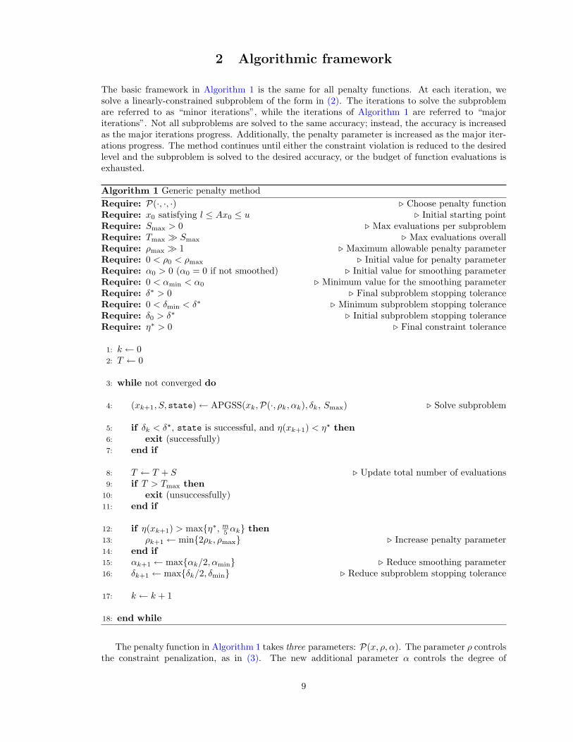
The basic framework in Algorithm 1 is the same for all penalty functions. At each iteration, wesolve a linearly-constrained subproblem of the form in (2). The iterations to solve the subproblemare referred to as “minor iterations”, while the iterations of Algorithm 1 are referred to “majoriterations”. Not all subproblems are solved to the same accuracy; instead, the accuracy is increasedas the major iterations progress. Additionally, the penalty parameter is increased as the major iter-ations progress. The method continues until either the constraint violation is reduced to the desiredlevel and the subproblem is solved to the desired accuracy, or the budget of function evaluations isexhausted.

Algorithm 1 Generic penalty methodRequire: P(·, ·, ·) . Choose penalty functionRequire: x0 satisfying l ≤ Ax0 ≤ u . Initial starting pointRequire: Smax > 0 . Max evaluations per subproblemRequire: Tmax Smax . Max evaluations overallRequire: ρmax 1 . Maximum allowable penalty parameterRequire: 0 < ρ0 < ρmax . Initial value for penalty parameterRequire: α0 > 0 (α0 = 0 if not smoothed) . Initial value for smoothing parameterRequire: 0 < αmin < α0 . Minimum value for the smoothing parameterRequire: δ∗ > 0 . Final subproblem stopping toleranceRequire: 0 < δmin < δ∗ . Minimum subproblem stopping toleranceRequire: δ0 > δ∗ . Initial subproblem stopping toleranceRequire: η∗ > 0 . Final constraint tolerance

1: k ← 02: T ← 0

3: while not converged do

4: (xk+1, S, state)← APGSS(xk,P(·, ρk, αk), δk, Smax) . Solve subproblem

5: if δk < δ?, state is successful, and η(xk+1) < η? then6: exit (successfully)7: end if

8: T ← T + S . Update total number of evaluations9: if T > Tmax then

10: exit (unsuccessfully)11: end if

12: if η(xk+1) > maxη∗, m5 αk then

13: ρk+1 ← min2ρk, ρmax . Increase penalty parameter14: end if15: αk+1 ← maxαk/2, αmin . Reduce smoothing parameter16: δk+1 ← maxδk/2, δmin . Reduce subproblem stopping tolerance

17: k ← k + 1

18: end while

The penalty function in Algorithm 1 takes three parameters: P(x, ρ, α). The parameter ρ controlsthe constraint penalization, as in (3). The new additional parameter α controls the degree of

9

smoothing for the smoothed exact penalty functions discussed in §4. It can be safely ignored forpenalty functions that do not require it by initializing α0 = 0.

At each major iteration, a linearly-constrained subproblem of the form in (2) is solved usingasynchronous, parallel GSS (APGSS) for linearly-constrained problems as described in [10]. Asinputs, it takes the solution of the last subproblem (xk), the penalty-based objective function withρ = ρk and α = αk, the stopping tolerance (δk), and the maximum number of function evaluationsallocated for the subproblem (Smax). The subproblem does a series of minor iterations until itconverges or exhausts the function evaluations. It returns the best point found, xk+1; the numberof function evaluations used, S; and a flag indicating whether or not the subproblem solver exitedsuccessfully, state.

An important factor is reducing the overall constraint violation, which is measured in terms ofthe maximum violation given by

η(x) = max | c+i (x) | , i = 1, . . . ,m. (4)

Consequently, η(x) plays a role in the convergence of the algorithm. Algorithm 1 is considered tohave exited successfully if the following three criteria are satisfied:

1. The subproblem stopping tolerance is less than the desired final tolerance δ?. Note that δk isallowed to drop below δ? but not below δmin.

2. The subproblem is solved successfully, meaning that APGSS successfully exited with a steplength tolerance of δk ≤ δ?.

3. The penalty parameter is large enough so that the maximum constraint violation, η(xk+1), isless than the specified threshold, η?.

Note also that the penalty parameter ρ is not increased if η(xk+1) is sufficiently small. Thoughthere are many options for controlling the reduction and growth rates of the penalty parameter,smoothing parameter, and stopping tolerance, we opted for a simple scheme because our primarygoal at this point is to directly compare different penalty functions and not the fine tuning of aparticular approach.

Detailed results and algorithmic settings are provided in Appendix A, and summary resultscomparing the number of function evaluations and final objective values are discussed in the sectionsthat follow. The test set comprised all CUTEr [8] problems with up to ten variables and betweenone and ten nonlinear constraints, for a total of 145 problems. A run for a given test problemand penalty function either terminates successfully (meaning, at a minimum, that η(x?) < η?) orunsuccessfully (e.g., because the number of function evaluations was exhausted). The number ofproblems in the union of all successful terminations is 128, so we use this in computing percentages ofproblems solved within a given number of function evaluations. Conversely, the number of problemsin the intersection is 98, and we restrict ourselves to these when comparing the relative accuracies.Note that since the subproblems are solved using the asynchronous method APGSS, we tested eachpenalty function multiple times and averaged the results. A penalty function is only reported to haveexited successfully if it did so on every run. Also, in comparing the number of function evaluations,note that APGSS caches the objective and constraint function values for re-use in future minor andeven major iterations, which means the same point will never be evaluated twice in the same run.Efficient re-use of previously evaluated points is critical for CS&E applications where evaluationsare expensive.

10

3 Exact penalty functions

Exact penalty methods are attractive because there exists a finite value of the penalty parameter ρsuch that that a minimizer (2) coincides with a solution to (1); see, e.g., [22]. On the other hand,a drawback for exact penalty functions based on primal variables (as opposed to dual variables)is that they are necessarily non-smooth at an optimal point [24]. For an in depth analysis of theoptimization of exact penalty functions, see Pillo and Grippo [26] and Pillo [25]. There are severaldefinitions for exact penalty functions in the literature. To avoid ambiguity, we use the followingdefinition from [26]:

Definition 3.1 The function P(x, ρ) is an exact penalty function for (1) with respect to a set Ω ifthere exists an ρ > 0 such that for all ρ > ρ, a global (local) unconstrained minimizer of

minx∈Ω

f(x) + P(x, ρ)

is a global (local) minimizer for (1).

Pillo and Grippo [26] further show that if the extended Mangasarian-Fromovitz constraint qual-ification is satisfied on Ω, then

P(x, ρ) = ρ‖c+(x)‖qis exact with respect to Ω for 1 ≤ q ≤ ∞. In this paper we explore properties of the following exactpenalty functions:

P`1(x, ρ) = ρ‖c+(x)‖1, (5)

P`2(x, ρ) = ρ‖c+(x)‖2, (6)

P`∞(x, ρ) = ρ‖c+(x)‖∞. (7)

Figure 1 shows two-dimensional contour plots for the `1, `2, `∞ and `22 penalty functions, cor-responding to two constraints. Dark blue indicates areas where the constraint violation penalty isvery small. The bigger this area is, the larger the penalty parameter has to be in order to reducethe constraint violation. Note that this dark blue area is relatively large for `22 and much smallerfor the three exact penalty functions. Conversely, the areas in red denote large penalties. Functionswith more red restrict the possible steps that the algorithms can take to obtain decrease until thepenalty parameter is very small. Once again, the `22 penalty function is the worst in this respect.

Overall the exact penalty functions are more attractive in that they allow larger steps for theGSS subproblem solver and do not require that the penalty parameter be increased exponentially tosufficiently reduce the constraint violation. For example, consider the `1 penalty function. Becauseit is linear in the constraint violation, it is possible to take relatively large steps yet decrease theobjective value. Furthermore, being linear in the constraint violation means that the penalty param-eter does not have to get asymptotically large to enforce constraint feasibility, once again enablinglarger steps. Thus, exact penalty functions permit GSS methods take larger steps than would bepermitted by `22. The downside, as Audet and Dennis [3] demonstrate, is that GSS methods appliedto exact penalty function can and do get stuck at points of non-differentiability.

The question is, how often does this happen in practice? Detailed numerical results for a collectionof 145 CUTEr test problems are presented in Appendix A. Exact penalty functions were pittedagainst the `22 penalty function. Recall from §2, that the general framework emphasizes constraintsatisfaction overall with η(xk+1) < η? being required, at a minimum, for a successful exit. In thesetests, η? = 10−3. Figure 2 presents summary results showing how many problems completed fora given number of function evaluations; Table 1 lists how many problems were solved in total. Asmentioned previously, the number of function evaluations should be as small as possible. Here we

11

Figure 1. Contours of various penalty function for two constraints.

see that the exact penalty methods are able to exit successfully in 1000 function evaluations or lessfor approximately 80% of the test problems. In contrast, `22, only solved 60% of the test problemswithin 1000 evaluations.

Penalty Number of function evaluationsFunction ≤ 1000 ≤ 2500 ≤ Tmax

`∞ 97 109 111`1 108 114 118`2 106 118 125`22 81 104 120

Table 1. Number of problems solved for each penalty function.

The number of function evaluations does not tell the entire story. Because of the constraint sat-isfaction requirement in the general framework, we are only comparing problems that have achievedsufficient feasibility, i.e., η(x) < η? = 10−3. But there are no explicit requirements on the objectivefunction value. Figure 3 shows the relative difference between the final objective function values forthe 98 test problems that all methods were able to solve. The relative difference is calculated as

f(x)− f(y)max1, |f(x)|, |f(y)|

, (8)

where x is the solution obtained using the `22 penalty function, and y is the solution obtained usingthe exact penalty function. Values greater than zero indicate that the exact method did better,whereas values less than zero indicate that the `22 method was better. Table 2 shows the percentageof problems that have the specified relative difference or better.

Observe that the exact penalty functions found better optima on a few problems. Moreover, theexact methods obtain an objective value that was no more than 10% worse than `22 on 84% of thetest problems.

Thus, we may be able to achieve lower overall objective values with `22, but at a higher costin terms of the number of function evaluations. Though there is the danger of the subproblem

12

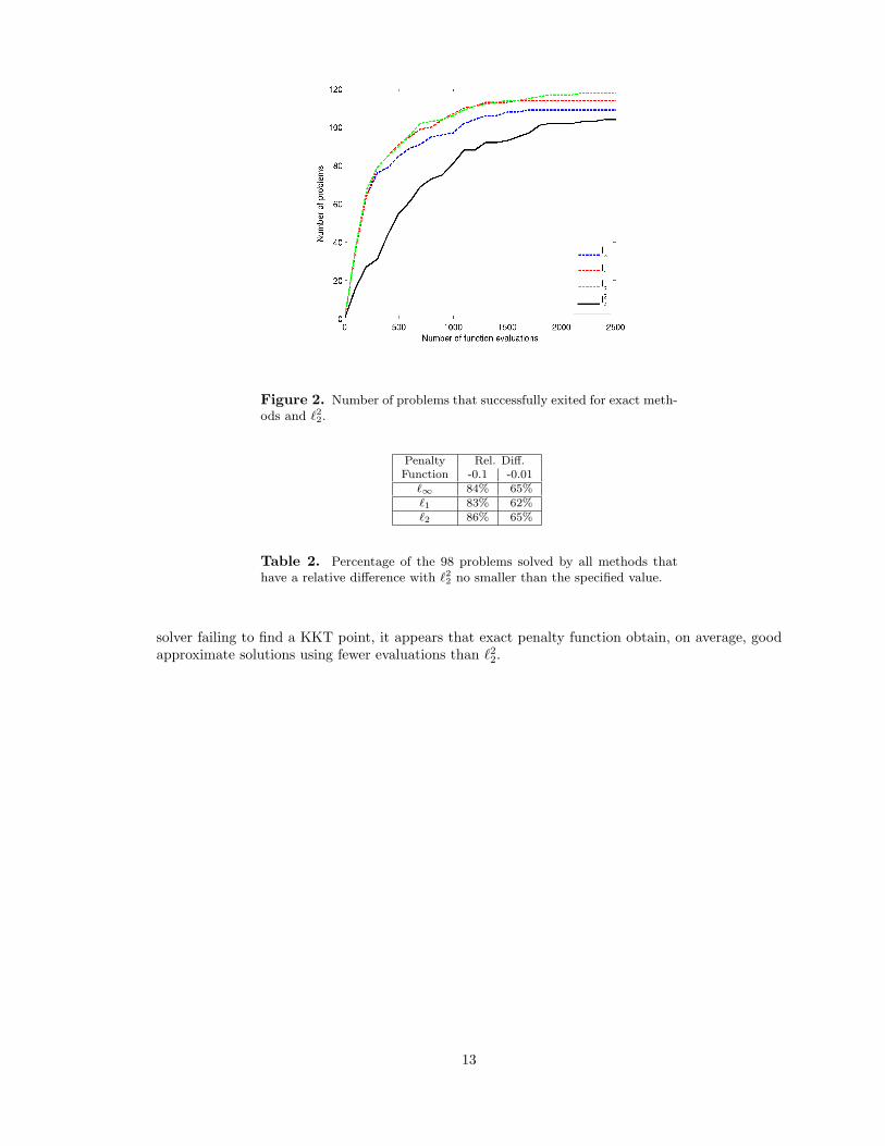
Figure 2. Number of problems that successfully exited for exact meth-ods and `22.

Penalty Rel. Diff.Function -0.1 -0.01

`∞ 84% 65%`1 83% 62%`2 86% 65%

Table 2. Percentage of the 98 problems solved by all methods thathave a relative difference with `22 no smaller than the specified value.

solver failing to find a KKT point, it appears that exact penalty function obtain, on average, goodapproximate solutions using fewer evaluations than `22.

13

Figure 3. Relative difference in final objective value compared to `22.

14

4 Smoothed exact penalty functions

Because GSS methods are derivative-free, they are naturally resilient to the non-smooth nature ofan exact penalty function in that there is no problem in executing the method. Yet, GSS methodsdo not guarantee global convergence to KKT points unless sufficient smoothness is present, perhapsexplaining why the final objective values for the exact penalty functions are not as good as thoseobtained by `22. Therefore, this section considers smoothed penalty functions that are variants of the`1, `2, and `∞ penalty functions. These penalty functions have a third parameter, α, that controlsthe degree of smoothing. Let S denote the smoothed version of the exact penalty function E . Eachof the penalty functions in this section satisfies the following properties:

1. S(x, ρ, α) > E(x, ρ) for α > 0,

2. | S(x, ρ, α)− E(x, ρ) | ≤ Cα for some constant C, independent of ρ, and

3. S(x, ρ, α) is smooth if c(x) is smooth.

The motivation for using smoothed penalty functions comes from the fact that the theory of GSSmethods (used to solve the linearly-constrained subproblems) requires that the objective functionbe continuously differentiable. Thus, it is hoped that a continuous objective function will improveoverall performance.

The smoothed version of the `1 penalty function used in this paper is based on Chen and Man-gasarian [4], who exploit the properties of the sigmoid function from neural networks to approxi-mate the sign function, integrating the sigmoid function to obtain a smooth approximation to the`1 penalty function. Their focus is on handling linear and convex inequalities. Spellucci [32] usethis same penalty function for the linear constraints in quadratic programming. The smoothed `1penalty function is defined as

Ps1(x, ρ, α) =∑i∈E

θ(ρci(x), α) +∑i∈I

ψ(ρci(x), α), (9)

where

θ(t, α) = α ln(2 + 2 cosh(t/α)),ψ(t, α) = α ln(1 + exp(t/α)).

The equality and inequality constrained are treated separately, though θ(t, α) is just ψ(t, α) +ψ(−t, α). Spellucci [32] proves the following bounds:

|t| < θ(t, α) < |t|+ 83αe−|t|/α,

t+ < ψ(t, α) < t+ +43αe−|t|/α.

This implies

ρ‖c+(x)‖1 < Ps1(x, ρ, α) < ρ‖c+(x)‖1 + 3mαe−ρη(x)/α ≤ ρ‖c+(x)‖1 + 3mα,

where η(x) = ‖c(x)‖∞.

The smoothed version of the `2 penalty function used in this paper relies on a positive shiftparameter to smooth the square-root function as in [5, 35, 27, 27, 34, 13, 36, 31], though of theseonly [5, 31] used this technique in the context of smoothing the `2 norm as described in §6. Thesmoothed version of the `2 penalty function is given by

Ps2(x, ρ, α) = ρ√‖c+(x)‖22 + (α/ρ)2. (10)

15

It is straightforward to show that

ρ‖c+(x)‖2 < Ps2(x, ρ, α) < ρ‖c+(x)‖2 +α2

max(ρ‖c+(x)‖2, α)≤ ρ‖c+(x)‖2 + α.

The smoothed version of the `∞ penalty function used in this paper was also used by [30, 37, 20,21]. Note that Liuzzi and Lucidi [20] and Liuzzi et al. [21] explore properties of this function in thecontext of derivative-free programming and also handle linear constraints explicitly. The smoothedversion of the `∞ penalty function is given by

Ps∞ = α ln

(1 +

∑i∈E

2 cosh(ρci(x)/α) +∑i∈I

eρci(x)/α

). (11)

Xu [37] proves the following error bound for the smoothing of the maximum violation norm:

ρ‖x‖∞ ≤ Ps∞(x, ρ, α) ≤ ρ‖x‖∞ + α ln(m).

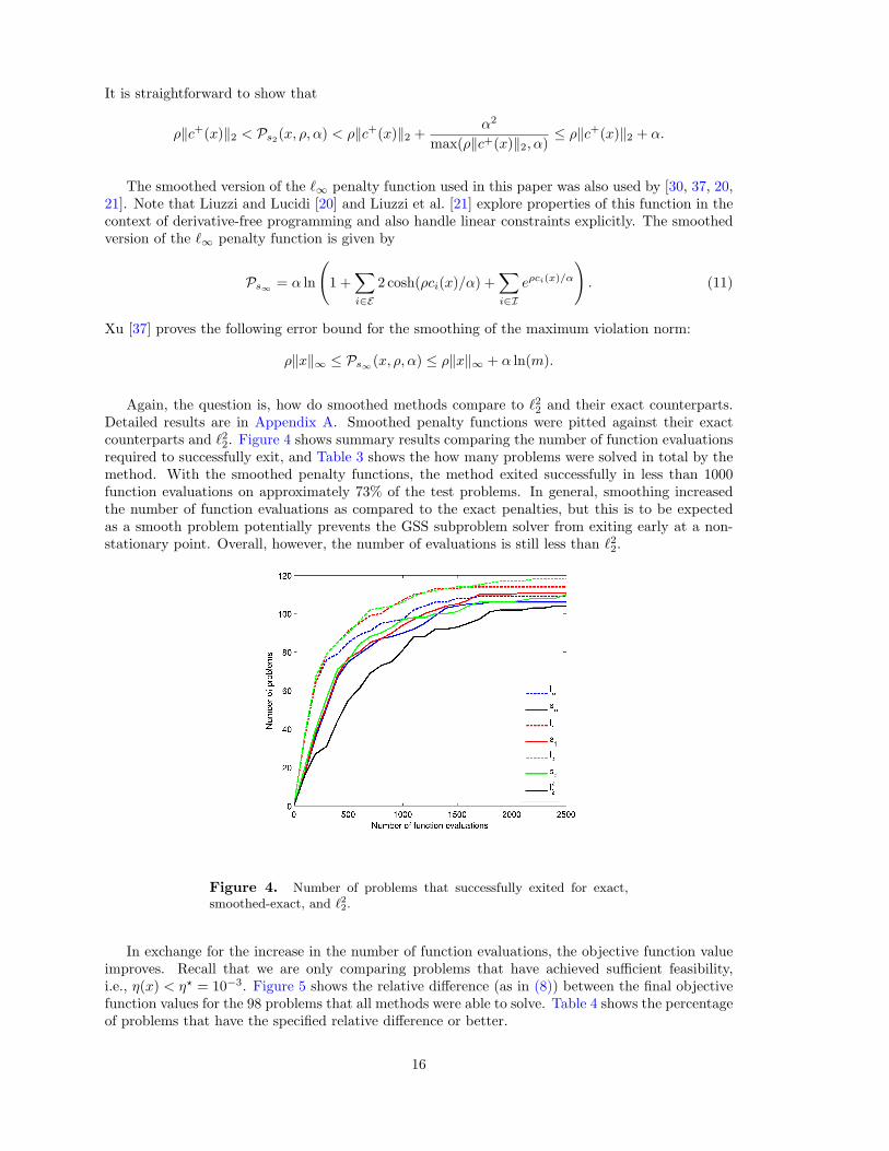
Again, the question is, how do smoothed methods compare to `22 and their exact counterparts.Detailed results are in Appendix A. Smoothed penalty functions were pitted against their exactcounterparts and `22. Figure 4 shows summary results comparing the number of function evaluationsrequired to successfully exit, and Table 3 shows the how many problems were solved in total by themethod. With the smoothed penalty functions, the method exited successfully in less than 1000function evaluations on approximately 73% of the test problems. In general, smoothing increasedthe number of function evaluations as compared to the exact penalties, but this is to be expectedas a smooth problem potentially prevents the GSS subproblem solver from exiting early at a non-stationary point. Overall, however, the number of evaluations is still less than `22.

Figure 4. Number of problems that successfully exited for exact,smoothed-exact, and `22.

In exchange for the increase in the number of function evaluations, the objective function valueimproves. Recall that we are only comparing problems that have achieved sufficient feasibility,i.e., η(x) < η? = 10−3. Figure 5 shows the relative difference (as in (8)) between the final objectivefunction values for the 98 problems that all methods were able to solve. Table 4 shows the percentageof problems that have the specified relative difference or better.

16

Penalty Number of function evaluationsFunction ≤ 1000 ≤ 2500 ≤ Tmax

s∞ 90 106 107s1 94 111 114s2 976 110 121

Table 3. Number of problems solved for each penalty function.

Figure 5. Relative difference in final objective value compared to `22.

The smoothed-exact penalty functions found even more improved optima that the exact penaltyfunction (these are reflected as positive relative differences in the graph). Moreover, the smoothed-exact methods obtain an objective value that was no more than 10% worse than `22 on approximately96% of the test problems.

Smoothed-exact penalty functions offer a potential compromise between obtaining a good objec-tive value and reducing the number of function evaluations. The smoothing parameter can poten-tially be adjusted to give better solution or fewer function evaluations, depending on the preferencesof the user.

Penalty Rel. Diff.Function -0.1 -0.01

s∞ 99% 85%s1 96% 80%s2 94% 79%

Table 4. Percentage of the 98 problems solved by all methods thathave a relative difference with `22 no smaller than the specified value.

17

This page intentionally left blank.

18

5 Theoretical underpinnings

In this section, we describe the theoretical underpinnings of penalty methods and how this relates tothe penalty functions in this paper. Classical theory on penalty methods does not separate the linearand nonlinear constraints as we do here, but the theory extends to this case in a straightforwardway. The following well-known theorem says that the sequence of approximate solutions to thesubproblem (2) converges to the solution of (1), provided that the penalty function satisfies certainconditions.

Theorem 5.1 (see, e.g., [22]) Assume that the penalty function P satisfies the following threeproperties for ρ ≥ 0:

1. P(x, ρ) is continuous,

2. P(x, ρ) > 0 for all c+(x) 6= 0, and

3. P(x, ρ) = 0 if and only if c+(x) = 0.

Let yk be a sequence of approximate solutions to (2) such that ‖yk − xk‖ → 0, where xk is anexact minimizer, as ρk → +∞. Then any limit point of the sequence yk is a solution to (1).

The penalty functions based on `22, `1, `2, and `∞ all satisfy the three required penalty functionproperties, but the smoothed variants discussed in §4 do not satisfy the third requirement.

Though the subproblems do not need to be solved exactly, Theorem 5.1 does require that the so-lutions must be increasingly good approximations. From [10], the measure of stationarity for (2) canbe bounded as a function of the step-length stopping tolerance if the merit function, f(x)+P(x, ρ, α),in (2) is continuously differentiable. Without linear constraints, this means that the norm of thegradient is bounded as a function of the stopping tolerance, i.e., δk in the outer loop. For linearconstraints, the norm of the gradient does not measure stationary, but there is an equivalent measureand bound with respect to the stopping tolerance. Thus, if the merit function is continuously differ-entiable, the approximate solutions to the subproblems will satisfy the conditions of Theorem 5.1,i.e., ‖yk − xk‖ → 0. If the merit function is not continuously differentiable, then the GSS methodwill still converge to a limit point, but it is no longer guaranteed to to have a small measure ofstationarity.

In this case, the `22 penalty functions and the three smoothed penalty functions are continuouslydifferentiable (provided f is also continuously differentiable), but the exact functions are not.

Consequently, it is well established that using the exact penalty functions may fail since there isno guarantee of obtaining a good approximate solution to the subproblem (2). Note that becausethe smooth penalty function are strictly greater than their exact counterparts, the third assumptionof Theorem 5.1 does not hold and hence we cannot directly apply Theorem 5.1.

Many researchers have investigated the convergence theory. Liuzzi and Lucidi [20] develop con-vergence theory for the smoothed-`∞ penalty function in the context of pattern search methodsand also handle the linear constraints explicitly. Kaplan [13] and Gonzaga and Castillo [7] developgeneral convergence theory for `1 smoothing functions in the context of nonlinear programming.Polyak [29] provides an extensive discussion on the general properties of smoothing techniques inthe context of the minimax function.

19

This page intentionally left blank.

20

6 Related Work

In §4 we described a particular choice of smoothing the `1 penalty function using integrals of thesigmoid function for neural networks proposed by Chen and Mangasarian [4] in the context ofhandling convex inequalities and linear complementarity problems. A nice feature of this approachis that the level of differentiability of the unconstrained problem is maintained. That is, the degreeof differentiability of M(x, ρ, α) is determined by the degree of differentiability of f(x) and c(x).Another popular choice for smoothing `1 is the use of linear-quadratic approximation such as theHuber penalty function [12] which is popular in the statistics community. Variants of piecewise linear-quadratic penalty functions are explored in the context of nonlinear programming in [35, 27, 28].Weber and Love [34], Kaplan [13] and Xavier [36] smooth the `1 penalty function using hyperboloidapproximation techniques, √

t2 + α and t+√t2 + α,

to approximate |t| and max0, t respectively. In §4, properties of this function are used to smooththe square-root term in the `2 norm.

In §4, we describe a smooth approximation for the `2 norm. Eyster, White, and Wierwille [5]use a similar strategy for minimizing a sum of Euclidean distances of the form

Fw(x) =K∑

i=1

‖x− wi‖2

in the context of solving the Euclidean Multifacility Location problem. Further properties of thisfunction in this context are explored by Ben and Xue [31]. There does not appear to be muchrelated work for smoothing the `2 norm in the context of general nonlinear programming; by far themajority of the literature focused on `1 and `∞.

Also of note is the algorithm proposed by Meng, Dang, and Yang [23] for using first and secondorder smoothing of the square-root exact penalty function,

M(x, ρ) = f(x) + ρm∑

i=1

√|c+i (x)|,

in the context of inequality constrained optimization.

The last smooth penalty function described in §4 approximates the `∞ function and has beenused in [30, 37, 20, 21]. Qin and Nguyen [30] first proposed using this smoothing in the context ofnonlinear programming. Xu [37] later used this penalty function to solve finite minimax problems.Liuzzi, Lucidi, and Sciandrone [21] developed a GSS approach to solving a linearly constrained finiteminimax problem.

We also explored a pseudo-smoothing of the `1 function using dynamic scaling:

P(x, ρ) =m∑

i=1

(1− η(x)− c+i (x)

η(x)

)︸ ︷︷ ︸

ξi(x)

c+i (x).

Recall that η(x) is the maximum constraint violation (4). The function ξi(x) = 0 if c+i (x) = 0, andξi(x) = 1 if c+i (x) = η(x), the maximum violation norm. An alternate formulation is given by

P(x, ρ) =∑

c+i (x)=η(x)

η(x) +∑

c+i (x)<η(x)

c+i (x)η(x)

c+i (x).

Hence this functions grows like `∞ for the largest constraint violations while damping the importanceof less violated constraints. This penalty function seemed effective for some of the more difficult

21

equality constrained problems, but on average did not perform as well as the penalty functionsdescribed in §4.

22

7 Conclusions

This paper focused on developing practical algorithms for solving real-world nonlinear programmingproblems in CS&E where the computational cost of each evaluation makes it prohibitive to performlarge numbers of function evaluations. The emphasis is on algorithms that are constraint centric;i.e., methods that exit with a feasible point are preferred to those that exit with an infeasible point,even if that infeasible point is closer to a KKT point.

We explored a variety of penalty methods in the context of derivative-free optimization, usingAPGSS to solve the subproblems on a parallel computer. These methods were tested on a collectionof CUTEr test problems with nonlinear constraints, as described in §2.

The `22 method has the best theoretical properties in that it is smooth and satisfies the require-ments of Theorem 5.1. However, it requires a large number of function evaluations relative to theother penalty functions.

The exact penalty functions discussed in §3 are not smooth and so GSS may converge to a pointof non-differentiability in the subproblem solution. But numerically, the exact penalty methodssuccessfully terminated on more problems than the other methods. Successful termination means,among other things, that the constraint violation is small The final objective values were not alwaysas good, however, as `22.

The smoothed-exact penalty functions discussed in §4 required slightly more function evaluations,but still less than `22. The trade-off is improved final objective values that are nearly always asaccurate at `22. The smoothing parameter can be adjusted to decide whether accuracy or efficiencyis more important.

The theory of penalty methods is discussed in §5, though we do not go into full details in thispaper. For future work, there are many other promising candidates (§6) for penalty functions thatmay be more appropriate in some application domains.

In conclusion, derivative-free penalty methods are a good option in the context of CS&E nonlinearprogramming problems. Using a penalty function that emphasizes constraint feasibility above allyields “usable” solutions even if they are not optimal in the KKT sense.

23

This page intentionally left blank.

24

A Detailed numerical results

Tables A.1–A.2 contain detailed numerical results for comparing the seven merit functions discussedin this paper. The code was run on five parallel processors (one controller plus four workers) onSandia’s Institutional Computing Cluster (ICC) with 3.06GHz Xeon processors and 2GB RAMper node. Because we were using an asynchronous algorithm to solve the linearly constrainedsubproblems, we ran each algorithm 5 times on each problem and averaged the results.

The following parameters were used for Algorithm 1:

• The starting point x0 is the default value given by CUTEr if it is feasible with respect to thelinear constraints. Otherwise, it is the solution to a feasibility problem with respect to thelinear constraints as in [9],

• Smax = 1000,

• Tmax = 100, 000,

• ρmax = 108,

• ρ0 = 1 ,

• αmin = 10−5,

• α0 = 1 ,

• δ? = 10−3,

• δmin = 10−6,

• δ0 = 10−1,

• η? = 10−3.

Additionally, the number of outer iterations was restricted to 1000. Default values were used forAPGSS, except for those parameters that are part of the algorithm; i.e., the starting point was setto the last outer iterate, the stopping tolerance for the step length was set to δk, and the maximumnumber of function evaluations was set to Smax.

The columns for Tables A.1–A.2 are as follows. The first column lists the problem name and itscharacteristics using the notation from (1). The second column lists the best objective value foundby any method that exited successfully. Note that a successful exit means that the constraints arenearly satisfied, i.e., η(x?) < η? = 10−3. The remaining seven columns list averaged results for eachmerit function. The first number is the relative difference as compared to the best minimum, i.e.,

∆f? =f(x?)− f?

min

max1, |f(x?)|, |f?min|

where f(x?) denotes the best objective value obtained by the corresponding method. The secondvalue (nf) is the number of objective/constraint function evaluations. Recall that APGSS cachesboth objective and constraint values and reuses them across inner and outer iterations in the samerun. Thus, these counts reflect unique points evaluated in the parameter space.

The seven merit functions that are compared are:

• `∞: see (7)

• s∞: see (11)

25

• `1: see (5)

• s1: see (9)

• `2: see (6)

• s2: see (10)

• `22: see (3)

Altogether, of the 145 problems, 128 were solved by at least one merit function, and 98 were solvedby all.

26

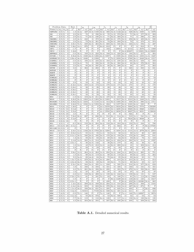
Problem Data Best `∞ s∞ `1 s1 `2 s2 `22Name/n/me/mi/p f? ∆f? / nf ∆f? / nf ∆f? / nf ∆f? / nf ∆f? / nf ∆f? / nf ∆f? / nf

CANTILVR/ 5/0/1/ 5 1.3 3e-2/ 427 4e-3/1108 3e-2/ 389 4e-3/1132 2e-2/ 428 8e-6/ 1065 0/ 1676

CB2 / 3/0/3/ 0 2.0 2e-2/ 70 0/ 336 2e-2/ 70 1e-3/ 372 2e-2/ 71 2e-2/ 377 2e-2/ 362

CB3 / 3/0/3/ 0 2.0 5e-4/ 71 4e-3/ 346 5e-4/ 71 6e-3/ 384 5e-4/ 71 0/ 386 0/ 364

CHACONN1/ 3/0/3/ 0 2.0 4e-3/ 243 0/ 373 4e-3/ 226 2e-3/ 375 3e-3/ 258 2e-3/ 483 2e-3/ 590

CHACONN2/ 3/0/3/ 0 2.0 5e-4/ 72 5e-3/ 361 5e-4/ 72 6e-3/ 393 5e-4/ 72 0/ 373 0/ 374

CONGIGMZ/ 3/0/2/ 3 2.8e1 7e-5/ 239 6e-5/ 263 8e-5/ 668 3e-5/ 500 6e-5/ 323 1e-5/ 592 0/ 487

CRESC4 / 6/0/8/ 5 1.8e1 1e-1/ 876 F/ F 8e-2/ 819 F/ F F/ F 0/ 816 F/ F

CSFI1 / 5/2/3/ 6 -1.7 F/ F F/ F 1/ 162 1/2004 0/ 2112 1/ 2470 1/ 1089

CSFI2 / 5/2/3/ 5 1.2e2 F/ F F/ F F/ F F/ F 3e-2/20407 0/19201 3e-2/18689

DEMYMALO/ 3/0/1/ 2 -3.0 3e-4/ 169 1e-3/ 222 3e-4/ 168 1e-3/ 223 2e-4/ 164 5e-5/ 217 0/ 364

DIPIGRI / 7/0/4/ 0 6.8e2 3e-3/ 1049 2e-3/1206 2e-3/1057 0/1585 6e-3/ 1008 5e-3/ 1655 1e-3/ 1627

DIXCHLNG/10/5/0/ 0 2.8e-4 4e-3/ 1646 0/1582 F/ F 7e-5/1659 4e-3/ 1766 2e-1/ 2449 2e-4/ 1517

GIGOMEZ1/ 3/0/1/ 2 -3.0 3e-4/ 189 1e-3/ 234 2e-4/ 183 1e-3/ 230 2e-4/ 184 3e-5/ 234 0/ 359

GIGOMEZ2/ 3/0/3/ 0 2.0 2e-2/ 70 0/ 326 2e-2/ 65 8e-4/ 360 2e-2/ 66 2e-2/ 376 2e-2/ 364

GIGOMEZ3/ 3/0/3/ 0 2.0 5e-4/ 66 4e-3/ 347 5e-4/ 66 6e-3/ 388 5e-4/ 66 0/ 377 0/ 363

GOTTFR / 2/2/0/ 0 0.0 0/ 302 0/ 250 F/ F F/ F 0/ 325 0/ 355 0/ 341

HATFLDF / 3/3/0/ 0 F F/ F F/ F F/ F F/ F F/ F F/ F F/ F

HEART6 / 6/6/0/ 0 F F/ F F/ F F/ F F/ F F/ F F/ F F/ F

HEART8 / 8/6/0/ 2 F F/ F F/ F F/ F F/ F F/ F F/ F F/ F

HIMMELBC/ 2/2/0/ 0 0.0 F/ F 0/ 52 0/ 52 0/ 51 0/ 51 0/ 51 0/ 52

HIMMELBD/ 2/2/0/ 0 F F/ F F/ F F/ F F/ F F/ F F/ F F/ F

HIMMELBE/ 3/1/0/ 2 0.0 0/ 23 0/ 23 0/ 23 0/ 23 0/ 23 0/ 23 0/ 23

HIMMELP2/ 2/0/1/ 4 -6.2e1 1e-6/ 169 1e-6/ 172 1e-6/ 170 1e-6/ 171 1e-6/ 170 0/ 171 0/ 170

HIMMELP3/ 2/0/2/ 4 -5.9e1 0/ 28 0/ 28 0/ 28 0/ 28 0/ 28 0/ 28 0/ 29

HIMMELP4/ 2/0/3/ 4 -5.9e1 0/ 42 0/ 41 0/ 44 0/ 42 0/ 42 0/ 48 0/ 44

HIMMELP5/ 2/0/3/ 4 -5.9e1 0/ 25 0/ 25 0/ 25 0/ 25 0/ 25 0/ 25 0/ 25

HIMMELP6/ 2/0/3/ 6 -5.9e1 0/ 22 0/ 22 0/ 22 0/ 22 0/ 22 0/ 22 0/ 22

HS10 / 2/0/1/ 0 -1.0 3e-4/ 102 4e-3/ 211 3e-4/ 105 4e-3/ 213 3e-4/ 100 1e-3/ 205 0/ 362

HS100 / 7/0/4/ 0 6.8e2 2e-3/ 1062 1e-3/1362 2e-3/1065 0/1617 2e-3/ 1010 2e-3/ 1449 1e-5/ 1799

HS100LNP/ 7/2/0/ 0 6.8e2 5e-3/ 1044 0/1144 1e-2/ 412 6e-3/1085 8e-3/ 639 3e-3/ 990 1e-2/ 1711

HS100MOD/ 7/0/4/ 0 6.8e2 7e-4/ 1020 1e-4/1359 9e-4/ 994 0/1377 9e-4/ 1035 8e-4/ 930 F/ F

HS101 / 7/0/6/ 14 1.8e3 F/ F F/ F 2e-1/5579 2e-1/5633 3e-2/ 7690 3e-2/ 7774 0/80390

HS102 / 7/0/6/ 14 9.1e2 F/ F F/ F 2e-1/4340 3e-1/4235 3e-2/ 6826 3e-2/ 6828 0/65614

HS103 / 7/0/6/ 14 5.5e2 F/ F F/ F 4e-1/3783 4e-1/3658 7e-2/ 6827 7e-2/ 6631 0/29032

HS104 / 8/0/6/ 16 4.0 F/ F F/ F F/ F F/ F 0/ 924 F/ F F/ F

HS106 / 8/0/3/ 19 7.6e3 3e-2/ 687 0/ 836 2e-1/ 510 2e-1/ 514 2e-1/ 519 1e-1/ 541 1e-1/ 593

HS107 / 9/6/0/ 8 5.1e3 F/ F F/ F F/ F F/ F 0/ 7818 2e-4/ 8068 F/ F

HS109 / 9/6/2/ 18 F F/ F F/ F F/ F F/ F F/ F F/ F F/ F

HS11 / 2/0/1/ 0 -8.5 3e-2/ 133 2e-3/ 204 3e-2/ 132 2e-3/ 203 3e-2/ 132 7e-3/ 249 0/ 786

HS111 /10/3/0/ 20 -4.1e1 F/ F F/ F F/ F 0/ 662 F/ F F/ F 8e-2/17590

HS111LNP/10/3/0/ 0 F F/ F F/ F F/ F F/ F F/ F F/ F F/ F

HS113 /10/0/5/ 3 2.4e1 1e-2/ 1182 3e-3/1702 2e-2/1256 0/1650 1e-2/ 1115 1e-3/ 2778 6e-3/ 2304

HS12 / 2/0/1/ 0 -3.0e1 1e-5/ 55 1e-5/ 55 1e-5/ 55 1e-5/ 56 1e-5/ 56 1e-5/ 80 0/ 400

HS13 / 2/0/1/ 2 8.1e-1 3e-3/ 180 2e-3/ 195 3e-3/ 179 2e-3/ 194 3e-3/ 179 2e-3/ 198 0/ 641

HS14 / 2/0/1/ 1 1.4 3e-3/ 59 3e-3/ 64 3e-3/ 60 3e-3/ 64 3e-3/ 59 2e-4/ 72 0/ 153

HS15 / 2/0/2/ 1 3.1e2 1e-3/ 560 1e-3/ 512 1e-3/ 622 1e-3/ 604 1e-3/ 560 1e-3/ 514 0/ 1027

HS16 / 2/0/2/ 3 2.5e-1 0/ 36 4e-5/ 142 0/ 36 6e-5/ 177 0/ 36 0/ 36 0/ 36

HS17 / 2/0/2/ 3 1.0 1e-3/ 43 7e-5/ 212 1e-3/ 44 6e-3/ 260 1e-3/ 43 0/ 202 1e-4/ 414

HS18 / 2/0/2/ 4 5.6 0/ 59 0/ 59 0/ 59 0/ 59 0/ 60 0/ 60 0/ 59

HS19 / 2/0/2/ 4 F F/ F F/ F F/ F F/ F F/ F F/ F F/ F

HS20 / 2/0/3/ 2 3.8e1 1e-3/ 264 1e-3/ 263 1e-3/ 250 1e-3/ 240 1e-3/ 263 1e-3/ 265 0/ 751

HS22 / 2/0/1/ 1 1.0 2e-3/ 88 4e-3/ 119 2e-3/ 88 4e-3/ 119 2e-3/ 89 6e-4/ 145 0/ 264

HS23 / 2/0/4/ 5 9.5 5e-2/ 69 4e-2/ 64 5e-2/ 70 4e-2/ 65 5e-2/ 69 4e-2/ 65 0/ 71

HS26 / 3/1/0/ 0 1.5e-7 2e-3/ 279 5e-2/ 313 4e-2/ 290 0/ 215 2e-3/ 313 2e-2/ 314 1/ 914

HS27 / 3/1/0/ 0 4.0e-2 3e-5/ 69 3e-5/ 69 3e-5/ 69 3e-5/ 71 3e-5/ 69 3e-5/ 69 0/ 417

HS29 / 3/0/1/ 0 -2.3e1 9e-2/ 244 5e-3/ 325 1e-1/ 228 0/ 325 7e-2/ 216 2e-2/ 277 2e-2/ 639

HS30 / 3/0/1/ 6 1.0 0/ 160 0/ 165 0/ 161 0/ 165 0/ 160 0/ 161 0/ 161

HS31 / 3/0/1/ 6 6.0 7e-3/ 281 8e-3/ 306 6e-3/ 290 0/ 303 7e-3/ 272 1e-4/ 300 8e-4/ 962

HS32 / 3/0/1/ 4 1.0 0/ 27 0/ 27 0/ 27 0/ 27 0/ 27 0/ 27 0/ 27

HS33 / 3/0/2/ 4 -4.6 1e-1/ 139 9e-4/ 289 1e-1/ 139 2e-3/ 242 1e-1/ 139 6e-2/ 131 0/ 537

HS34 / 3/0/2/ 6 -7.2e-1 7e-1/ 81 0/ 181 7e-1/ 83 0/ 180 7e-1/ 81 7e-1/ 113 4e-1/ 1065

HS39 / 4/2/0/ 0 -1.0 F/ F F/ F F/ F 8e-4/1429 2e-3/ 118 2e-3/ 125 0/ 3417

HS40 / 4/3/0/ 0 -2.5e-1 F/ F F/ F 0/ 430 F/ F 8e-4/ 432 2e-1/41680 3e-4/ 965

HS42 / 4/1/0/ 1 1.4e1 2e-2/ 299 4e-3/ 408 2e-2/ 294 1e-3/ 310 2e-2/ 299 5e-3/ 368 0/ 1034

HS43 / 4/0/3/ 0 -4.4e1 2e-3/ 509 0/ 683 8e-3/ 378 9e-4/ 844 1e-3/ 487 3e-3/ 874 F/ F

HS46 / 5/2/0/ 0 1.1e-3 4e-2/ 438 3e-2/ 621 1e-1/ 395 0/ 625 1e-1/ 405 F/ F 2e-2/ 686

HS47 / 5/3/0/ 0 3.4e-6 1/31915 1/7109 3e-3/ 598 5e-6/ 491 1e-2/ 611 F/ F 0/ 453

HS56 / 7/4/0/ 0 -3.5 7e-1/ 140 F/ F 7e-1/ 140 F/ F 7e-1/ 140 7e-1/44967 0/ 3074

HS57 / 2/0/1/ 2 3.1e-2 0/ 55 9e-6/ 572 0/ 53 9e-6/ 566 0/ 52 0/ 53 0/ 53

HS59 / 2/0/3/ 4 -7.7 3e-2/ 119 0/ 116 8e-2/ 129 0/ 117 1e-1/ 132 5e-2/ 123 8e-2/ 130

HS6 / 2/1/0/ 0 4.5 8e-2/ 204 8e-2/ 205 0/ 207 8e-2/ 206 8e-2/ 204 0/ 206 8e-2/ 206

Table A.1. Detailed numerical results

27

Problem Data Best `∞ s∞ `1 s1 `2 s2 `22Name/n/me/mi/p f? ∆f? / nf ∆f? / nf ∆f? / nf ∆f? / nf ∆f? / nf ∆f? / nf ∆f? / nf

HS60 /3/1/0/ 6 1.4e1 0/ 401 2e-1/ 444 2e-1/ 446 2e-1/ 444 3e-1/ 512 2e-1/ 442 7e-1/ 766

HS61 /3/2/0/ 0 -1.4e2 4e-3/ 88 6e-3/ 413 4e-3/ 90 7e-4/ 450 4e-3/ 88 0/ 376 2e-4/ 836

HS63 /3/1/0/ 4 9.6e2 5e-4/ 177 0/ 205 5e-4/ 185 5e-4/ 171 5e-4/ 186 2e-4/ 206 2e-4/ 459

HS64 /3/0/1/ 3 6.3e3 6e-4/2722 F/ F 6e-4/2755 F/ F 6e-4/ 2729 6e-4/ 2700 0/17169

HS65 /3/0/1/ 6 9.7e-1 2e-1/ 183 2e-2/ 233 2e-1/ 185 2e-2/ 232 2e-1/ 189 2e-1/ 188 0/ 431

HS66 /3/0/2/ 6 5.3e-1 4e-2/ 100 6e-3/ 639 4e-2/ 100 4e-2/ 138 4e-2/ 99 4e-2/ 139 0/ 422

HS68 /4/2/0/ 8 -3.7e-1 8e-4/ 195 8e-5/ 452 8e-4/ 201 8e-5/ 457 8e-4/ 192 8e-4/ 195 0/ 650

HS69 /4/2/0/ 8 -9.5e2 F/ F F/ F 1e-3/ 624 0/ 724 2e-3/ 758 2e-3/ 759 F/ F

HS7 /2/1/0/ 0 -1.7 2e-2/ 91 2e-2/ 133 2e-2/ 91 1e-2/ 160 2e-2/ 91 2e-2/ 149 0/ 197

HS70 /4/0/1/ 8 1.9e-1 4e-6/ 181 7e-6/ 184 7e-6/ 185 0/ 175 0/ 176 4e-6/ 180 1e-5/ 189

HS71 /4/1/1/ 8 1.7e1 7e-2/ 352 7e-2/ 186 9e-2/ 328 2e-1/ 465 6e-2/ 344 2e-2/ 302 0/ 566

HS72 /4/0/2/ 8 6.9e2 5e-2/ 738 6e-2/ 715 6e-2/ 790 6e-2/ 778 3e-3/ 626 3e-3/ 626 0/ 2873

HS73 /4/0/1/ 6 3.0e1 0/ 204 5e-6/ 196 1e-4/ 169 5e-5/ 180 8e-5/ 171 3e-3/ 224 5e-4/ 373

HS74 /4/3/0/ 10 5.1e3 F/ F F/ F F/ F F/ F F/ F F/ F 0/ 1258

HS75 /4/3/0/ 10 5.2e3 F/ F F/ F F/ F F/ F 0/ 1482 F/ F F/ F

HS77 /5/2/0/ 0 8.4e-1 3e-1/ 511 0/1073 6e-1/ 492 3e-1/ 904 9e-2/ 530 9e-2/ 555 2e-1/ 1519

HS78 /5/3/0/ 0 -2.8 F/ F F/ F 9e-2/ 829 0/ 991 2e-1/ 921 9e-2/ 960 4e-1/ 1058

HS79 /5/3/0/ 0 9.0e-2 4e-1/ 774 0/ 743 9e-1/ 511 1e-1/ 986 5e-1/ 681 1e-1/ 815 1e-1/ 946

HS8 /2/2/0/ 0 -1.0 0/ 182 F/ F F/ F F/ F 0/ 279 0/ 277 0/ 243

HS80 /5/3/0/ 10 9.7e-2 0/1133 4e-2/1007 3e-1/ 916 3e-1/1127 1e-1/ 1316 4e-2/ 1253 3e-2/ 1072

HS81 /5/3/0/ 10 7.0e-2 1/1259 F/ F 9e-1/1150 F/ F 9e-1/ 1696 9e-1/ 1596 0/ 1018

HS83 /5/0/6/ 10 -3.1e4 9e-3/ 445 9e-3/ 444 2e-4/ 204 2e-4/ 205 3e-6/ 216 3e-6/ 208 0/ 2122

HS84 /5/0/6/ 10 -5.2e6 1e-1/1209 1e-1/1205 1e-1/ 881 1e-1/ 857 2e-1/ 699 2e-1/ 695 0/ 683

HS87 /6/4/0/ 12 F F/ F F/ F F/ F F/ F F/ F F/ F F/ F

HS88 /2/0/1/ 0 1.1 4e-2/ 455 5e-2/ 528 5e-2/ 431 5e-2/ 540 4e-2/ 457 5e-2/ 543 0/ 1278

HS89 /3/0/1/ 0 1.1 5e-2/ 640 5e-2/ 679 5e-2/ 666 5e-2/ 699 5e-2/ 662 5e-2/ 680 0/ 1862

HS90 /4/0/1/ 0 1.1 5e-2/ 920 5e-2/ 930 5e-2/ 903 5e-2/ 994 5e-2/ 867 5e-2/ 984 0/ 2516

HS91 /5/0/1/ 0 1.1 5e-2/1052 5e-2/1277 5e-2/1059 5e-2/1337 5e-2/ 1133 5e-2/ 1226 0/ 3094

HS92 /6/0/1/ 0 1.1 5e-2/1418 5e-2/1492 4e-2/1274 5e-2/1554 5e-2/ 1280 5e-2/ 1587 0/ 3676

HS93 /6/0/2/ 6 F F/ F F/ F F/ F F/ F F/ F F/ F F/ F

HS95 /6/0/4/ 12 1.6e-2 0/ 101 1e-4/ 327 0/ 101 1e-4/ 328 0/ 101 2e-1/ 101 0/ 102

HS96 /6/0/4/ 12 1.6e-2 0/ 101 1e-4/ 328 0/ 101 1e-4/ 329 0/ 101 0/ 100 0/ 101

HS97 /6/0/4/ 12 4.1 1e-3/ 184 0/ 177 1e-3/ 184 0/ 177 0/ 185 1e-3/ 438 2e-4/ 840

HS98 /6/0/4/ 12 4.1 0/ 185 0/ 176 0/ 185 0/ 175 0/ 184 1e-3/ 499 1e-3/ 918

HS99 /7/2/0/ 14 F F/ F F/ F F/ F F/ F F/ F F/ F F/ F

HYPCIR /2/2/0/ 0 0.0 F/ F 0/ 254 0/ 234 0/ 223 0/ 228 0/ 245 0/ 235

KIWCRESC/3/0/2/ 0 -9.8e-4 1e-3/ 78 5e-3/ 363 1e-3/ 78 8e-3/ 360 1e-3/ 78 0/ 364 3e-4/ 485

LEWISPOL/6/6/0/ 15 1.1 3e-5/ 350 3e-5/ 358 0/ 338 2e-5/ 336 1e-4/ 349 2e-4/ 342 1e-4/ 354

LOOTSMA /3/0/2/ 4 1.4 5e-1/ 50 5e-1/ 50 5e-1/ 50 5e-1/ 50 5e-1/ 50 0/ 178 5e-1/ 50

LSNNODOC/5/0/0/ 10 1.2e2 0/ 99 0/ 101 0/ 101 0/ 102 0/ 102 0/ 100 0/ 103

MADSEN /3/0/6/ 0 6.2e-1 4e-1/ 65 6e-3/ 459 4e-1/ 65 9e-3/ 444 4e-1/ 65 3e-4/ 612 0/ 619

MAKELA1 /3/0/1/ 1 -1.4 3e-3/ 252 3e-3/ 344 3e-3/ 242 3e-3/ 343 3e-3/ 239 4e-3/ 315 0/ 938

MAKELA2 /3/0/3/ 0 7.2 5e-1/ 164 4e-2/ 711 2e-1/ 118 0/ 413 2e-5/ 118 3e-2/ 402 4e-2/ 571

MARATOS /2/1/0/ 0 -1.0 3e-2/ 88 3e-2/ 135 3e-2/ 89 2e-2/ 137 3e-2/ 89 1e-3/ 168 0/ 199

MATRIX2 /6/0/2/ 4 0.0 0/ 100 0/ 100 0/ 100 0/ 100 0/ 100 0/ 100 0/ 100

MIFFLIN1/3/0/1/ 1 -1.0 2e-1/ 71 2e-4/ 146 2e-1/ 72 3e-4/ 164 2e-1/ 70 2e-4/ 334 0/ 477

MIFFLIN2/3/0/2/ 0 -1.0 8e-1/ 79 3e-3/ 329 8e-1/ 79 3e-3/ 308 8e-1/ 79 2e-4/ 582 0/ 620

MINMAXRB/3/0/2/ 2 -9.0e-15 1/ 160 4e-2/1105 1/ 160 4e-2/1088 1/ 159 1/ 160 0/13442

MWRIGHT /5/3/0/ 0 1.3 2e-1/ 785 0/1378 5e-1/ 850 4e-2/1216 1/20577 1/26200 9e-2/ 1258

PFIT1 /3/3/0/ 0 F F/ F F/ F F/ F F/ F F/ F F/ F F/ F

PFIT2 /3/3/0/ 0 F F/ F F/ F F/ F F/ F F/ F F/ F F/ F

PFIT3 /3/3/0/ 0 F F/ F F/ F F/ F F/ F F/ F F/ F F/ F

PFIT4 /3/3/0/ 0 F F/ F F/ F F/ F F/ F F/ F F/ F F/ F

POLAK1 /3/0/2/ 0 2.7 7e-1/ 744 2e-3/ 730 7e-1/ 440 4e-3/ 872 7e-1/ 502 1e-4/ 2093 0/ 1484

POLAK4 /3/0/3/ 0 -8.0e-4 7e-2/ 216 8e-3/ 373 7e-2/ 235 1e-2/ 388 7e-2/ 214 5e-4/ 337 0/ 456

POLAK5 /3/0/2/ 0 5.0e1 8e-3/1461 7e-4/1230 8e-3/1561 1e-3/1152 4e-3/ 1844 0/ 1505 8e-5/ 1791

POLAK6 /5/0/4/ 0 -4.4e1 9e-1/ 136 2e-4/ 909 9e-1/ 133 0/1022 9e-1/ 140 8e-2/ 2136 7e-2/ 2503

POWELLBS/2/2/0/ 0 0.0 F/ F F/ F F/ F F/ F F/ F 0/10281 F/ F

POWELLSQ/2/2/0/ 0 0.0 0/ 47 0/ 47 0/ 47 0/ 47 0/ 47 0/ 47 0/ 47

RECIPE /3/2/0/ 1 0.0 0/ 59 0/ 59 0/ 60 0/ 59 0/ 59 0/ 59 0/ 59

ROSENMMX/5/0/4/ 0 -4.4e1 1/ 100 2e-2/1320 1/ 100 0/1213 1/ 100 2e-1/ 1622 2e-1/ 1772

S316-322/2/1/0/ 0 3.3e2 8e-3/ 595 8e-3/ 595 5e-3/ 600 9e-3/ 602 6e-3/ 597 8e-3/ 592 0/ 5811

S365 /7/0/5/ 4 0.0 F/ F 0/ 164 0/ 225 0/ 167 0/ 171 0/ 171 0/ 171

S365MOD /7/0/5/ 4 F F/ F F/ F F/ F F/ F F/ F F/ F F/ F

SNAKE /2/0/2/ 0 3.5e-1 2e-1/ 177 F/ F 0/ 203 F/ F 2e-1/ 177 F/ F F/ F

SPIRAL /3/0/2/ 0 -4.9e-4 1e-1/ 132 F/ F 1e-1/ 244 F/ F 1e-1/ 220 F/ F 0/83125

SYNTHES1/6/0/2/ 16 7.6e-1 3e-3/ 404 3e-3/ 457 3e-3/ 361 3e-3/ 475 3e-3/ 386 2e-4/ 581 0/ 1253

TRIGGER /7/3/0/ 5 F F/ F F/ F F/ F F/ F F/ F F/ F F/ F

TRY-B /2/1/0/ 2 0.0 1/ 56 0/ 88 1/ 56 0/ 83 1/ 56 0/ 100 0/ 86

TWOBARS /2/0/2/ 4 1.5 1e-2/ 128 3e-3/ 202 1e-2/ 126 1e-3/ 155 1e-2/ 126 2e-3/ 289 0/ 547

WOMFLET /3/0/3/ 0 -7.6e-4 8e-4/ 150 1e-2/ 424 8e-4/ 129 1e-2/ 300 8e-4/ 132 0/ 719 3e-5/ 633

ZECEVIC3/2/0/2/ 4 9.8e1 2e-2/ 199 1e-2/ 207 2e-2/ 198 1e-2/ 210 2e-2/ 198 1e-2/ 204 0/ 462

ZECEVIC4/2/0/1/ 5 7.6 7e-3/ 201 5e-3/ 187 6e-3/ 188 5e-3/ 185 6e-3/ 189 4e-3/ 146 0/ 735

ZY2 /3/0/2/ 4 2.0 2e-3/ 153 2e-3/ 129 2e-3/ 154 2e-3/ 130 2e-3/ 153 2e-3/ 152 0/ 305

Table A.2. Detailed numerical results

28

References

[1] C. Audet and J. E. Dennis, Jr., Mesh adaptive direct search algorithms for constrainedoptimization, SIAM J. Optimiz., 17 (2006), pp. 188–217.

[2] C. Audet and J. E. Dennis, Jr., Analysis of generalized pattern searches, SIAM J. Optimiz.,13 (2003), pp. 889–903.

[3] C. Audet and J. E. Dennis, Jr., A pattern search filter method for nonlinear programmingwithout derivatives, SIAM J. Optimiz., 14 (2004), pp. 980–1010.

[4] C. Chen and O. L. Mangasarian, Smoothing methods for convex inequalities and linearcomplementarity problems, Math. Program., 71 (1995), pp. 51–69.

[5] J. Eyster, J. White, and W. Wierwille, On solving multifacility location problems usinga hyperboloid approximation procedure., AIIE Transactions, 5 (1973), pp. 1–6.

[6] A. V. Fiacco and G. P. McCormick, Nonlinear Programming: Sequential UnconstrainedMinimization Techniques, John Wiley & Sons, New York, NY, USA, 1968. Reprint : Volume 4of SIAM Classics in Applied Mathematics, SIAM Publications, Philadelphia, PA 19104–2688,USA, 1990.

[7] C. C. Gonzaga and R. A. Castillo, A nonlinear programming algorithm based on non-coercive penalty functions, Math. Program., 96 (2003), pp. 87–101.

[8] N. I. M. Gould, D. Orban, and Ph. L. Toint, CUTEr and SifDec: a constrained andunconstrained testing environment, revisited, ACM T. Math. Software, 29 (2003), pp. 373–394.

[9] G. A. Gray and T. G. Kolda, Algorithm 856: APPSPACK 4.0: Asynchronous parallelpattern search for derivative-free optimization, ACM T. Math. Software, 32 (2006), pp. 485–507.

[10] J. D. Griffin, T. G. Kolda, and R. M. Lewis, Asynchronous parallel generating set searchfor linearly-constrained optimization, Tech. Report SAND2006-4621, Sandia National Labora-tories, Albuquerque, New Mexico and Livermore, California, Aug. 2006.

[11] P. D. Hough, T. G. Kolda, and V. J. Torczon, Asynchronous parallel pattern search fornonlinear optimization, SIAM J. Sci. Comput., 23 (2001), pp. 134–156.

[12] P. J. Huber, Robust Statistics, Wiley, 1981.

[13] A. A. Kaplan, Convex programming algorithms using smoothing of exact penalty functions,Siberian Mathematical Journal, 23 (1982), pp. 491–500.

[14] T. G. Kolda, Revisiting asynchronous parallel pattern search for nonlinear optimization, SIAMJ. Optimiz., 16 (2005), pp. 563–586.

[15] T. G. Kolda, R. M. Lewis, and V. Torczon, Optimization by direct search: new perspec-tives on some classical and modern methods, SIAM Rev., 45 (2003), pp. 385–482.

[16] T. G. Kolda, R. M. Lewis, and V. Torczon, A generating set direct search augmentedLagrangian algorithm for optimization with a combination of general and linear constraints,Tech. Report SAND2006-5315, Sandia National Laboratories, Albuquerque, New Mexico andLivermore, California, Aug. 2006.

[17] R. M. Lewis and V. Torczon, Pattern search algorithms for bound constrained minimization,SIAM J. Optimiz., 9 (1999), pp. 1082–1099.

[18] R. M. Lewis and V. Torczon, Pattern search methods for linearly constrained minimization,SIAM J. Optimiz., 10 (2000), pp. 917–941.

29

[19] R. M. Lewis and V. Torczon, A globally convergent augmented Lagrangian pattern searchalgorithm for optimization with general constraints and simple bounds, SIAM J. Optimiz., 12(2002), pp. 1075–1089.

[20] G. Liuzzi and S. Lucidi, A derivative-free algorithm for nonlinear programming, Tech. ReportTR 17/05, Department of Computer and Systems Science ”Antonio Ruberti”, University ofRome ”La Sapienza”, 2005.

[21] G. Liuzzi, S. Lucidi, and M. Sciandrone, A derivative-free algorithm for linearly con-strained finite minimax problems, SIAM J. Optimiz., 16 (2006), pp. 1054–1075.

[22] D. G. Luenberger, Linear and Nonlinear Programming, Addison-Wesley, 2nd ed., 1989.

[23] Z. Meng, C. Dang, and X. Yang, On the smoothing of the square-root exact penalty functionfor inequality constrained optimization, Comput. Optim. Appl., 35 (2006), pp. 375–398.

[24] J. Nocedal and S. J. Wright, Numerical Optimization, Springer, 1999.

[25] G. D. Pillo, Exact penalty methods, in Algorithms for Continuous Optimization: the State ofthe Art, E. Spedicato, ed., Kluwer, 1994, pp. 1–45.

[26] G. D. Pillo and L. Grippo, On the exactness of a class of nondifferentiable penalty functions,J. Optim. Theory Appl., 57 (1988), pp. 399–410.

[27] M. C. Pinar and S. A. Zenios, A data-level parallel linear-quadratic penalty algorithm formulticommodity network flows, ACM Trans. Math. Softw., 20 (1994), pp. 531–552.

[28] , On smoothing exact penalty functions for convex constrained optimization, SIAM J. Op-timiz., 4 (1994), pp. 486–511.

[29] R. Polyak, I. Griva, and J. Sobieski, Nonlinear rescaling in discrete minimax, in Nons-mooth/Nonconvex Mechanic: Modeling, Analaysis and Numerical Methods, D. Gao, R. Ogden,and G. Stavroulakis, eds., Kluwer, 2000, pp. 235–265.

[30] J. Qin and D. T. Nguyen, Generalized exponential penalty function for nonlinear program-ming, in AIAA/ASME/ASCE/AHS/ASC Structures, Structural Dynamics, and Materials Con-ference, 35th, Hilton Head, SC, Apr 18-20, 1994, Technical Papers. Pt. 1 (A94-23876 06-39),Washington, DC, American Institute of Aeronautics and Astronautics, p. 411-416, 1994.

[31] J. Rosen and G. Xue, On the convergence of a hyperboloid approximation procedure for theperturbed euclidean multifacility location problem, Operations Research, 41 (1993), pp. 1164–1171.

[32] P. Spellucci, Solving QP problems by penalization and smoothing, Preprint 2242, TUD Dept.of Math., 2002.

[33] V. Torczon, On the convergence of pattern search algorithms, SIAM J. Optimiz., 7 (1997),pp. 1–25.

[34] G. Wesolowsky and R. Love, A nonlinear approximation method for solving a generalizedrectangular distance weber problem., Management Science, 18(11) (1972), pp. 656–663.

[35] Z. Y. Wu, H. W. J. Lee, F. Bai, and L. Zhang, Quadratic smoothing approximation to l1exact penalty function in global optimization, Journal of Industrial and Management Optimiza-tion, 1 (2005), pp. 533–547.

[36] A. E. Xavier, Hyperbolic penalty: A new method for nonlinear programming with inequalities.,International Transactions in Operational Research, 8 (2001), pp. 659–671.

[37] S. Xu, Smoothing method for minimax problems, Computational Optimization and Applica-tions, 20 (2001), pp. 267–279.

30

v1.23