nonparametric estimation: part ii - stanford universityyjhan/nonparametric... · nonparametric...

Nonparametric Estimation: Part IIRegression in Transformed Space

Yanjun Han

Department of Electrical EngineeringStanford University

[email protected]

November 20, 2015

Outline

1 Transformed space: Gaussian sequence estimation

2 Estimation via Fourier transformEstimation in Sobolev ellipsoidsAdaptive estimation over ellipsoidsDiscussions

3 Estimation via wavelet transformIntroduction to waveletsIntroduction to Besov spaceVisuShrink estimatorSureShrink estimatorGeneral Lr riskExperiments

4 Miscellaneous

2 / 72

Gaussian white noise model

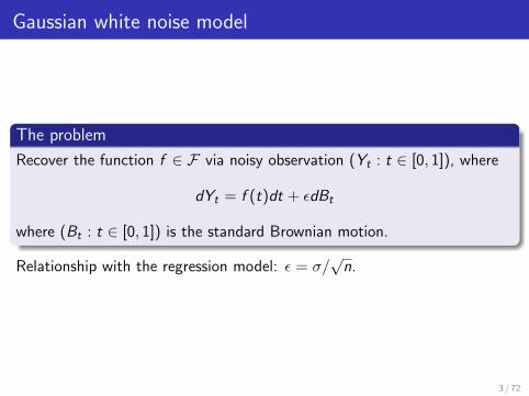
The problem

Recover the function f ∈ F via noisy observation (Yt : t ∈ [0, 1]), where

dYt = f (t)dt + εdBt

where (Bt : t ∈ [0, 1]) is the standard Brownian motion.

Relationship with the regression model: ε = σ/√n.

3 / 72

Gaussian sequence estimation

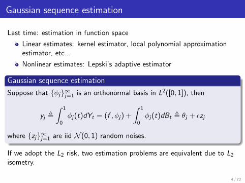
Last time: estimation in function space

Linear estimates: kernel estimator, local polynomial approximationestimator, etc...

Nonlinear estimates: Lepski’s adaptive estimator

Gaussian sequence estimation

Suppose that {φj}∞j=1 is an orthonormal basis in L2([0, 1]), then

yj ,∫ 1

0φj(t)dYt = (f , φj) +

∫ 1

0φj(t)dBt , θj + εzj

where {zj}∞j=1 are iid N (0, 1) random noises.

If we adopt the L2 risk, two estimation problems are equivalent due to L2

isometry.

4 / 72

Projection estimator

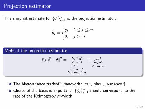
The simplest estimate for {θj}∞j=1 is the projection estimator:

θj =

{yj , 1 ≤ j ≤ m

0, j > m

MSE of the projection estimator

Eθ‖θ − θ‖2 =∑j>m

θ2j︸︷︷︸

Squared Bias

+ mε2︸︷︷︸Variance

The bias-variance tradeoff: bandwidth m ↑, bias ↓, variance ↑Choice of the basis is important: {φj}mj=1 should correspond to therate of the Kolmogorov m-width

5 / 72




4 Miscellaneous

6 / 72

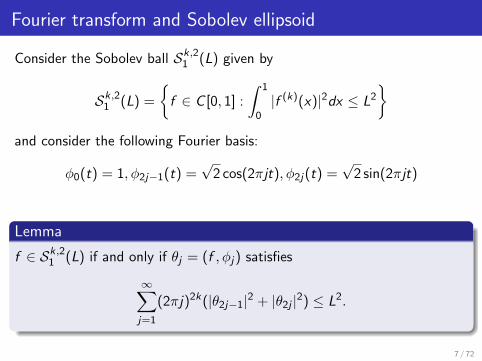
Fourier transform and Sobolev ellipsoid

Consider the Sobolev ball Sk,21 (L) given by

Sk,21 (L) =

{f ∈ C [0, 1] :

∫ 1

0|f (k)(x)|2dx ≤ L2

}and consider the following Fourier basis:

φ0(t) = 1, φ2j−1(t) =√

2 cos(2πjt), φ2j(t) =√

2 sin(2πjt)

Lemma

f ∈ Sk,21 (L) if and only if θj = (f , φj) satisfies

∞∑j=1

(2πj)2k(|θ2j−1|2 + |θ2j |2) ≤ L2.

7 / 72

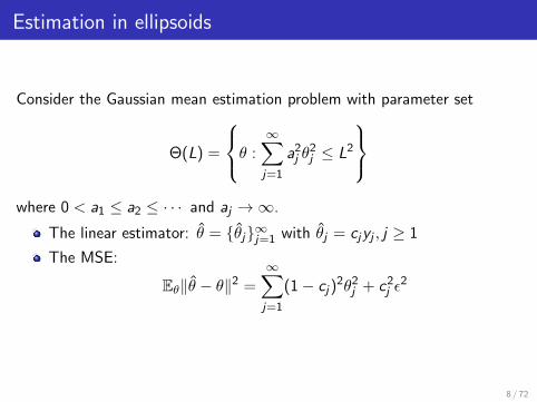
Estimation in ellipsoids

Consider the Gaussian mean estimation problem with parameter set

Θ(L) =

θ :∞∑j=1

a2j θ

2j ≤ L2

where 0 < a1 ≤ a2 ≤ · · · and aj →∞.

The linear estimator: θ = {θj}∞j=1 with θj = cjyj , j ≥ 1

The MSE:

Eθ‖θ − θ‖2 =∞∑j=1

(1− cj)2θ2

j + c2j ε

2

8 / 72

Minimax linear estimator

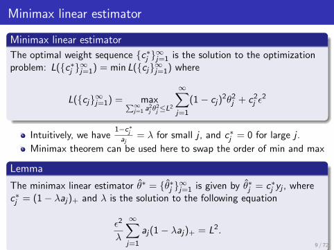
Minimax linear estimator

The optimal weight sequence {c∗j }∞j=1 is the solution to the optimizationproblem: L({c∗j }∞j=1) = min L({cj}∞j=1) where

L({cj}∞j=1) = max∑∞j=1 a

2j θ

2j ≤L2

∞∑j=1

(1− cj)2θ2

j + c2j ε

2

Intuitively, we have1−c∗jaj

= λ for small j , and c∗j = 0 for large j .

Minimax theorem can be used here to swap the order of min and max

Lemma

The minimax linear estimator θ∗ = {θ∗j }∞j=1 is given by θ∗j = c∗j yj , wherec∗j = (1− λaj)+ and λ is the solution to the following equation

ε2

λ

∞∑j=1

aj(1− λaj)+ = L2.

9 / 72

Pinsker’s theorem

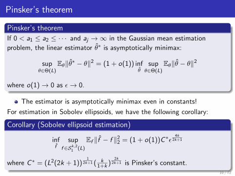
Pinsker’s theorem

If 0 < a1 ≤ a2 ≤ · · · and aj →∞ in the Gaussian mean estimation

problem, the linear estimator θ∗ is asymptotically minimax:

supθ∈Θ(L)

Eθ‖θ∗ − θ‖2 = (1 + o(1)) infθ

supθ∈Θ(L)

Eθ‖θ − θ‖2

where o(1)→ 0 as ε→ 0.

The estimator is asymptotically minimax even in constants!

For estimation in Sobolev ellipsoids, we have the following corollary:

Corollary (Sobolev ellipsoid estimation)

inff

supf ∈Sk,21 (L)

Ef ‖f − f ‖22 = (1 + o(1))C ∗ε

4k2k+1

where C ∗ = (L2(2k + 1))1

2k+1 ( k1+k )

2k2k+1 is Pinsker’s constant.

10 / 72




4 Miscellaneous

11 / 72

James-Stein estimator

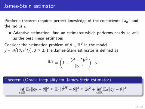
Pinsker’s theorem requires perfect knowledge of the coefficients {an} andthe radius L

Adaptive estimation: find an estimator which performs nearly as wellas the best linear estimates

Consider the estimation problem of θ ∈ Rd in the modely ∼ N (θ, ε2Id), d ≥ 3, the James-Stein estimator is defined as

θJS =

(1− (d − 2)ε2

‖y‖2

)+

y

Theorem (Oracle inequality for James-Stein estimator)

infc∈R

Eθ‖cy − θ‖2 ≤ Eθ‖θJS − θ‖2 ≤ 2ε2 + infc∈R

Eθ‖cy − θ‖2

12 / 72

Block James-Stein estimator

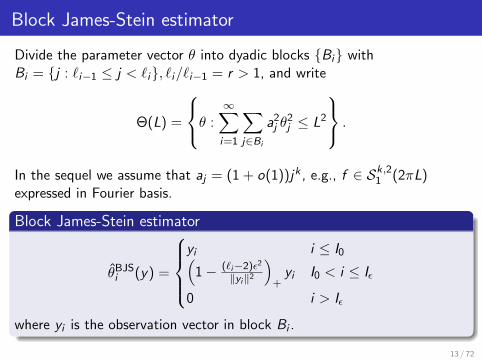
Divide the parameter vector θ into dyadic blocks {Bi} withBi = {j : ì−1 ≤ j < ì}, ì/ì−1 = r > 1, and write

Θ(L) =

θ :∞∑i=1

∑j∈Bi

a2j θ

2j ≤ L2

.

In the sequel we assume that aj = (1 + o(1))jk , e.g., f ∈ Sk,21 (2πL)expressed in Fourier basis.

Block James-Stein estimator

θBJSi (y) =

yi i ≤ I0(

1− (ì−2)ε2

‖yi‖2

)+yi I0 < i ≤ Iε

0 i > Iε

where yi is the observation vector in block Bi .

13 / 72

Choice of the threshold

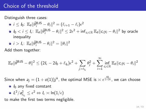
Distinguish three cases:

i ≤ I0: Eθ‖θBJSi − θi‖2 = (ì+1 − ì )ε2

I0 < i ≤ Iε: Eθ‖θBJSi − θi‖2 ≤ 2ε2 + infci∈R Eθ‖ciyi − θi‖2 by oracle

inequality

i > Iε: Eθ‖θBJSi − θi‖2 = ‖θi‖2

Add them together:

Eθ‖θBJS − θ‖2 ≤ (2Iε − 2I0 + Ì0)ε2 +∑j>Ìε

θ2j +

∞∑i=1

infci∈R

Eθ‖ciyi − θi‖2

Since when aj = (1 + o(1))jk , the optimal MSE is � ε4k

1+2k , we can choose

I0 any fixed constant

L2/a2Ìε≤ ε2 ⇔ Iε � ln(1/ε)

to make the first two terms negligible.

14 / 72

Performance of block James-Stein estimator

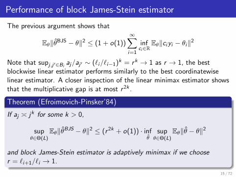
The previous argument shows that

Eθ‖θBJS − θ‖2 ≤ (1 + o(1))∞∑i=1

infci∈R

Eθ‖ciyi − θi‖2

Note that supj ,j ′∈Biaj/aj ′ ∼ (ì/ì−1)k = rk → 1 as r → 1, the best

blockwise linear estimator performs similarly to the best coordinatewiselinear estimator. A closer inspection of the linear minimax estimator showsthat the multiplicative gap is at most r2k .

Theorem (Efroimovich-Pinsker’84)

If aj � jk for some k > 0,

supθ∈Θ(L)

Eθ‖θBJS − θ‖2 ≤ (r2k + o(1)) · infθ

supθ∈Θ(L)

Eθ‖θ − θ‖2

and block James-Stein estimator is adaptively minimax if we chooser = ì+1/ì → 1.

15 / 72




4 Miscellaneous

16 / 72

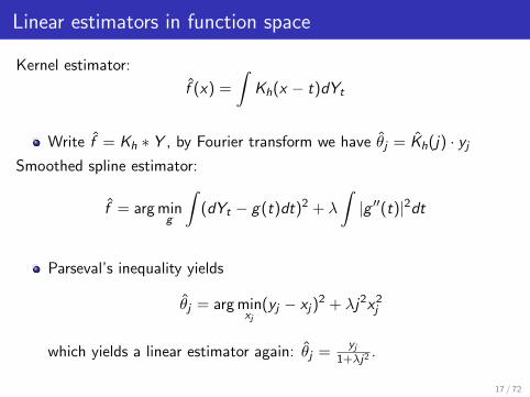
Linear estimators in function space

Kernel estimator:

f (x) =

∫Kh(x − t)dYt

Write f = Kh ∗ Y , by Fourier transform we have θj = Kh(j) · yjSmoothed spline estimator:

f = arg ming

∫(dYt − g(t)dt)2 + λ

∫|g ′′(t)|2dt

Parseval’s inequality yields

θj = arg minxj

(yj − xj)2 + λj2x2

j

which yields a linear estimator again: θj =yj

1+λj2 .

17 / 72

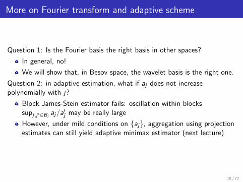
More on Fourier transform and adaptive scheme

Question 1: Is the Fourier basis the right basis in other spaces?

In general, no!

We will show that, in Besov space, the wavelet basis is the right one.

Question 2: in adaptive estimation, what if aj does not increasepolynomially with j?

Block James-Stein estimator fails: oscillation within blockssupj ,j ′∈Bi

aj/a′j may be really large

However, under mild conditions on {aj}, aggregation using projectionestimates can still yield adaptive minimax estimator (next lecture)

18 / 72




4 Miscellaneous

19 / 72

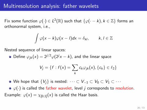
Multiresolution analysis: father wavelets

Fix some function ϕ(·) ∈ L2(R) such that {ϕ(· − k), k ∈ Z} forms anorthonormal system, i.e.,∫

ϕ(x − k)ϕ(x − l)dx = δkl , k , l ∈ Z

Nested sequence of linear spaces:

Define ϕjk(x) = 2j/2ϕ(2jx − k), and the linear space

Vj = {f : f (x) =∑k

ckϕjk(x), {ck} ∈ `2}

We hope that {Vj} is nested: · · · ⊂ V−1 ⊂ V0 ⊂ V1 ⊂ · · ·ϕ(·) is called the father wavelet, level j corresponds to resolution.

Example: ϕ(x) = χ[0,1](x) is called the Haar basis.

20 / 72

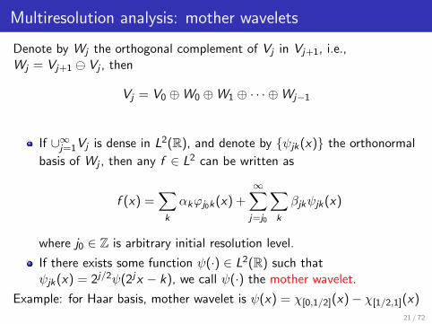
Multiresolution analysis: mother wavelets

Denote by Wj the orthogonal complement of Vj in Vj+1, i.e.,Wj = Vj+1 Vj , then

Vj = V0 ⊕W0 ⊕W1 ⊕ · · · ⊕Wj−1

If ∪∞j=1Vj is dense in L2(R), and denote by {ψjk(x)} the orthonormal

basis of Wj , then any f ∈ L2 can be written as

f (x) =∑k

αkϕj0k(x) +∞∑j=j0

∑k

βjkψjk(x)

where j0 ∈ Z is arbitrary initial resolution level.

If there exists some function ψ(·) ∈ L2(R) such thatψjk(x) = 2j/2ψ(2jx − k), we call ψ(·) the mother wavelet.

Example: for Haar basis, mother wavelet is ψ(x) = χ[0,1/2](x)− χ[1/2,1](x)

21 / 72

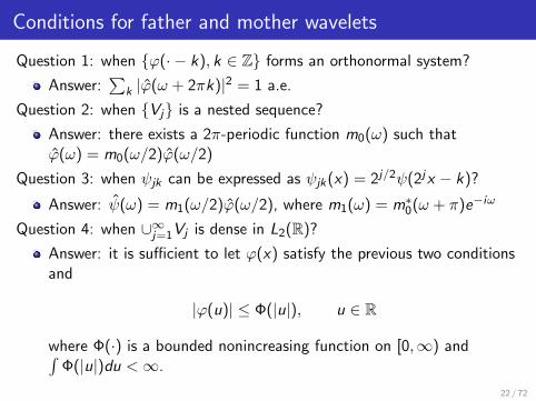
Conditions for father and mother wavelets

Question 1: when {ϕ(· − k), k ∈ Z} forms an orthonormal system?

Answer:∑

k |ϕ(ω + 2πk)|2 = 1 a.e.

Question 2: when {Vj} is a nested sequence?

Answer: there exists a 2π-periodic function m0(ω) such thatϕ(ω) = m0(ω/2)ϕ(ω/2)

Question 3: when ψjk can be expressed as ψjk(x) = 2j/2ψ(2jx − k)?

Answer: ψ(ω) = m1(ω/2)ϕ(ω/2), where m1(ω) = m∗0(ω + π)e−iω

Question 4: when ∪∞j=1Vj is dense in L2(R)?

Answer: it is sufficient to let ϕ(x) satisfy the previous two conditionsand

|ϕ(u)| ≤ Φ(|u|), u ∈ R

where Φ(·) is a bounded nonincreasing function on [0,∞) and∫Φ(|u|)du <∞.

22 / 72

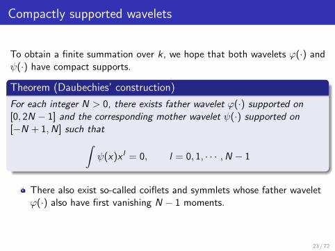
Compactly supported wavelets

To obtain a finite summation over k , we hope that both wavelets ϕ(·) andψ(·) have compact supports.

Theorem (Daubechies’ construction)

For each integer N > 0, there exists father wavelet ϕ(·) supported on[0, 2N − 1] and the corresponding mother wavelet ψ(·) supported on[−N + 1,N] such that∫

ψ(x)x l = 0, l = 0, 1, · · · ,N − 1

There also exist so-called coiflets and symmlets whose father waveletϕ(·) also have first vanishing N − 1 moments.

23 / 72

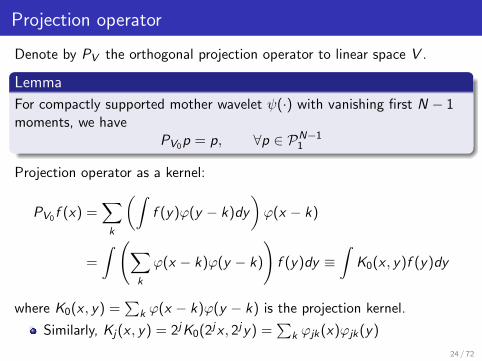
Projection operator

Denote by PV the orthogonal projection operator to linear space V .

Lemma

For compactly supported mother wavelet ψ(·) with vanishing first N − 1moments, we have

PV0p = p, ∀p ∈ PN−11

Projection operator as a kernel:

PV0f (x) =∑k

(∫f (y)ϕ(y − k)dy

)ϕ(x − k)

=

∫ (∑k

ϕ(x − k)ϕ(y − k)

)f (y)dy ≡

∫K0(x , y)f (y)dy

where K0(x , y) =∑

k ϕ(x − k)ϕ(y − k) is the projection kernel.

Similarly, Kj(x , y) = 2jK0(2jx , 2jy) =∑

k ϕjk(x)ϕjk(y)

24 / 72

Approximation by wavelets

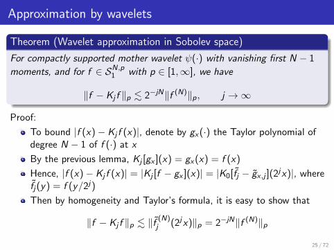
Theorem (Wavelet approximation in Sobolev space)

For compactly supported mother wavelet ψ(·) with vanishing first N − 1

moments, and for f ∈ SN,p1 with p ∈ [1,∞], we have

‖f − Kj f ‖p . 2−jN‖f (N)‖p, j →∞

Proof:

To bound |f (x)− Kj f (x)|, denote by gx(·) the Taylor polynomial ofdegree N − 1 of f (·) at x

By the previous lemma, Kj [gx ](x) = gx(x) = f (x)

Hence, |f (x)− Kj f (x)| = |Kj [f − gx ](x)| = |K0[fj − gx ,j ](2jx)|, wherefj(y) = f (y/2j)

Then by homogeneity and Taylor’s formula, it is easy to show that

‖f − Kj f ‖p . ‖f (N)j (2jx)‖p = 2−jN‖f (N)‖p

25 / 72




4 Miscellaneous

26 / 72

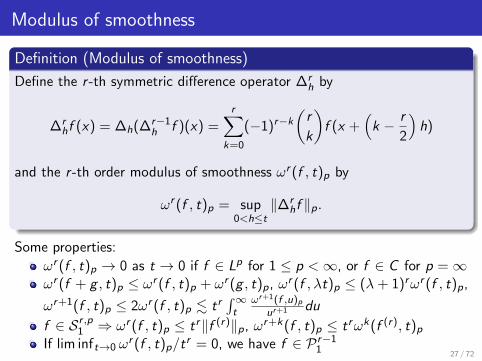
Modulus of smoothness

Definition (Modulus of smoothness)

Define the r -th symmetric difference operator ∆rh by

∆rhf (x) = ∆h(∆r−1

h f )(x) =r∑

k=0

(−1)r−k(r

k

)f (x +

(k − r

2

)h)

and the r -th order modulus of smoothness ωr (f , t)p by

ωr (f , t)p = sup0<h≤t

‖∆rhf ‖p.

Some properties:

ωr (f , t)p → 0 as t → 0 if f ∈ Lp for 1 ≤ p <∞, or f ∈ C for p =∞ωr (f + g , t)p ≤ ωr (f , t)p + ωr (g , t)p, ωr (f , λt)p ≤ (λ+ 1)rωr (f , t)p,

ωr+1(f , t)p ≤ 2ωr (f , t)p . tr∫∞t

ωr+1(f ,u)pur+1 du

f ∈ Sr ,p1 ⇒ ωr (f , t)p ≤ tr‖f (r)‖p, ωr+k(f , t)p ≤ trωk(f (r), t)pIf lim inft→0 ω

r (f , t)p/tr = 0, we have f ∈ P r−1

1 27 / 72

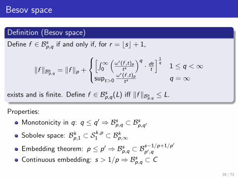
Besov space

Definition (Besov space)

Define f ∈ Bsp,q if and only if, for r = bsc+ 1,

‖f ‖Bsp,q = ‖f ‖p +

[∫∞

0

(ωr (f ,t)p

ts

)q· dtt] 1

q1 ≤ q <∞

supt>0ωr (f ,t)p

ts q =∞

exists and is finite. Define f ∈ Bsp,q(L) iff ‖f ‖Bsp,q ≤ L.

Properties:

Monotonicity in q: q ≤ q′ ⇒ Bsp,q ⊂ Bsp,q′

Sobolev space: Bkp,1 ⊂ Sk,p1 ⊂ Bkp,∞

Embedding theorem: p ≤ p′ ⇒ Bsp,q ⊂ Bs−1/p+1/p′

p′,q

Continuous embedding: s > 1/p ⇒ Bsp,q ⊂ C

28 / 72

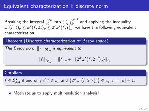
Equivalent characterization I: discrete norm

Breaking the integral∫∞

0 into∑

j

∫ 2j+1

2j and applying the inequalityωr (f , t)p ≤ ωr (f , 2t)p ≤ 2rωr (f , t)p, we have the following equivalentcharacterization.

Theorem (Discrete characterization of Besov space)

The Besov norm ‖ · ‖Bsp,q is equivalent to

‖f ‖Bsp,q = ‖f ‖p + ‖{2jsωr (f , 2−j)p}‖`q

Corollary

f ∈ Bsp,q if and only if f ∈ Lp and {2jsωr (f , 2−j)p} ∈ `q, r = bsc+ 1.

Motivate us to apply multiresolution analysis!

29 / 72

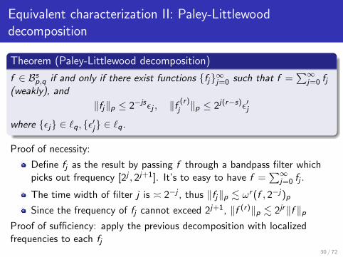
Equivalent characterization II: Paley-Littlewooddecomposition

Theorem (Paley-Littlewood decomposition)

f ∈ Bsp,q if and only if there exist functions {fj}∞j=0 such that f =∑∞

j=0 fj(weakly), and

‖fj‖p ≤ 2−jsεj , ‖f (r)j ‖p ≤ 2j(r−s)ε′j

where {εj} ∈ `q, {ε′j} ∈ `q.

Proof of necessity:

Define fj as the result by passing f through a bandpass filter whichpicks out frequency [2j , 2j+1]. It’s to easy to have f =

∑∞j=0 fj .

The time width of filter j is � 2−j , thus ‖fj‖p . ωr (f , 2−j)p

Since the frequency of fj cannot exceed 2j+1, ‖f (r)‖p . 2jr‖f ‖pProof of sufficiency: apply the previous decomposition with localizedfrequencies to each fj

30 / 72

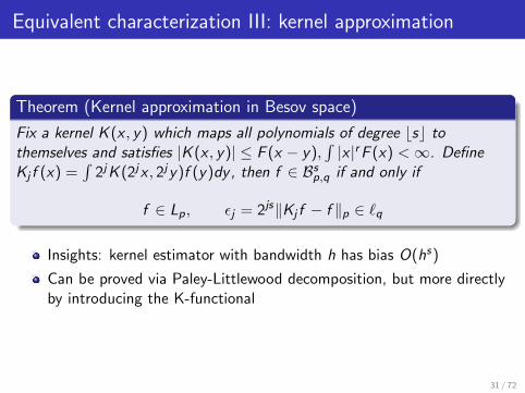
Equivalent characterization III: kernel approximation

Theorem (Kernel approximation in Besov space)

Fix a kernel K (x , y) which maps all polynomials of degree bsc tothemselves and satisfies |K (x , y)| ≤ F (x − y),

∫|x |rF (x) <∞. Define

Kj f (x) =∫

2jK (2jx , 2jy)f (y)dy , then f ∈ Bsp,q if and only if

f ∈ Lp, εj = 2js‖Kj f − f ‖p ∈ `q

Insights: kernel estimator with bandwidth h has bias O(hs)

Can be proved via Paley-Littlewood decomposition, but more directlyby introducing the K-functional

31 / 72

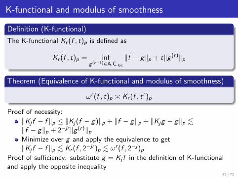
K-functional and modulus of smoothness

Definition (K-functional)

The K-functional Kr (f , t)p is defined as

Kr (f , t)p = infg (r−1)∈A.C.loc

‖f − g‖p + t‖g (r)‖p

Theorem (Equivalence of K-functional and modulus of smoothness)

ωr (f , t)p � Kr (f , tr )p

Proof of necessity:

‖Kj f − f ‖p ≤ ‖Kj(f − g)‖p + ‖f − g‖p + ‖Kjg − g‖p .‖f − g‖p + 2−jr‖g (r)‖pMinimize over g and apply the equivalence to get‖Kj f − f ‖p . Kr (f , 2−jr )p . ωr (f , 2−j)p

Proof of sufficiency: substitute g = Kj f in the definition of K-functionaland apply the opposite inequality

32 / 72

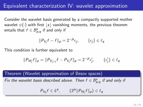
Equivalent characterization IV: wavelet approximation

Consider the wavelet basis generated by a compactly supported motherwavelet ψ(·) with first bsc vanishing moments, the previous theorementails that f ∈ Bsp,q if and only if

‖PVjf − f ‖p = 2−jsεj , {εj} ∈ `q

This condition is further equivalent to

‖PWjf ‖p = ‖PVj+1

f − PVjf ‖p = 2−jsε′j , {ε′j} ∈ `q

Theorem (Wavelet approximation of Besov spaces)

Fix the wavelet basis described above. Then f ∈ Bsp,q if and only if

PV0f ∈ Lp, {2js‖PWjf ‖p} ∈ `q

33 / 72

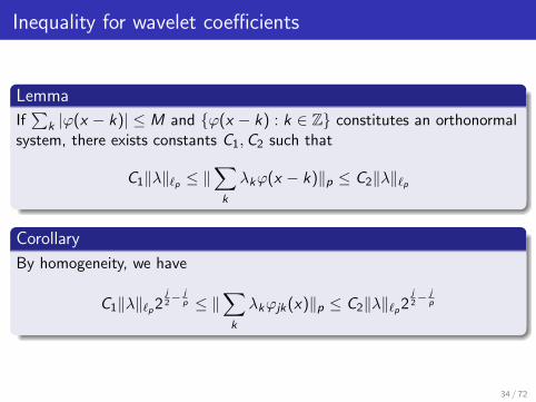
Inequality for wavelet coefficients

Lemma

If∑

k |ϕ(x − k)| ≤ M and {ϕ(x − k) : k ∈ Z} constitutes an orthonormalsystem, there exists constants C1,C2 such that

C1‖λ‖`p ≤ ‖∑k

λkϕ(x − k)‖p ≤ C2‖λ‖`p

Corollary

By homogeneity, we have

C1‖λ‖`p2j2− j

p ≤ ‖∑k

λkϕjk(x)‖p ≤ C2‖λ‖`p2j2− j

p

34 / 72

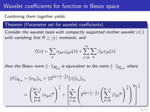
Wavelet coefficients for function in Besov space

Combining them together yields:

Theorem (Parameter set for wavelet coefficients)

Consider the wavelet basis with compactly supported mother wavelet ψ(·)with vanishing first R ≥ bsc moments, and

f (x) =∑k

αj0kϕj0k(x) +∞∑j=j0

∑k

βjkψjk(x)

then the Besov norm ‖ · ‖Bsp,q

is equivalent to the norm ‖ · ‖bsp,q , where

‖f ‖bsp,q = ‖αj0‖`p + ‖2j(s+ 12− 1

p)‖βj‖`p‖`q

=

2j0−1∑k=0

|αj0k |p

1p

+

∞∑j=j0

2j(s+ 12− 1

p)

2j−1∑k=0

|βjk |p 1

p

q

1q

35 / 72




4 Miscellaneous

36 / 72

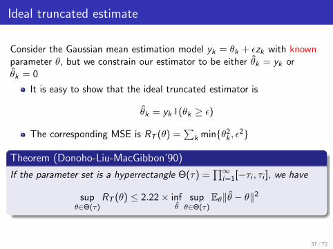
Ideal truncated estimate

Consider the Gaussian mean estimation model yk = θk + εzk with knownparameter θ, but we constrain our estimator to be either θk = yk orθk = 0

It is easy to show that the ideal truncated estimator is

θk = yk1(θk ≥ ε)

The corresponding MSE is RT (θ) =∑

k min{θ2k , ε

2}

Theorem (Donoho-Liu-MacGibbon’90)

If the parameter set is a hyperrectangle Θ(τ) =∏∞

i=1[−τi , τi ], we have

supθ∈Θ(τ)

RT (θ) ≤ 2.22× infθ

supθ∈Θ(τ)

Eθ‖θ − θ‖2

37 / 72

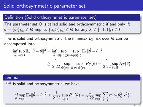
Solid orthosymmetric parameter set

Definition (Solid orthosymmetric parameter set)

The parameter set Θ is called solid and orthosymmetric if and only if:θ = {θi}i∈I ∈ Θ implies {λiθi}i∈I ∈ Θ for any λi ∈ [−1, 1], i ∈ I .

If Θ is solid and orthosymmetric, the minimax L2 risk over Θ can bedecomposed into

infθ

supθ∈Θ

Eθ‖θ − θ‖2 = infθ

supΘ(τ)⊂Θ

supθ∈Θ(τ)

Eθ‖θ − θ‖2

≥ 1

2.22sup

Θ(τ)⊂Θsup

θ∈Θ(τ)RT (θ) =

1

2.22supθ∈Θ

RT (θ)

Lemma

If Θ is solid and orthosymmetric, we have

infθ

supθ∈Θ

Eθ‖θ − θ‖2 ≥ 1

2.22supθ∈Θ

RT (θ) =1

2.22supθ∈Θ

∑k∈I

min{θ2k , ε

2}

38 / 72

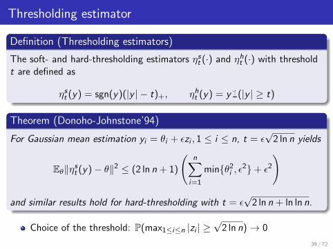
Thresholding estimator

Definition (Thresholding estimators)

The soft- and hard-thresholding estimators ηst (·) and ηht (·) with thresholdt are defined as

ηst (y) = sgn(y)(|y | − t)+, ηht (y) = y1(|y | ≥ t)

Theorem (Donoho-Johnstone’94)

For Gaussian mean estimation yi = θi + εzi , 1 ≤ i ≤ n, t = ε√

2 ln n yields

Eθ‖ηst (y)− θ‖2 ≤ (2 ln n + 1)

(n∑

i=1

min{θ2i , ε

2}+ ε2

)

and similar results hold for hard-thresholding with t = ε√

2 ln n + ln ln n.

Choice of the threshold: P(max1≤i≤n |zi | ≥√

2 ln n)→ 0

39 / 72

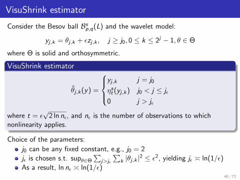
VisuShrink estimator

Consider the Besov ball Bsp,q(L) and the wavelet model:

yj ,k = θj ,k + εzj ,k , j ≥ j0, 0 ≤ k ≤ 2j − 1, θ ∈ Θ

where Θ is solid and orthosymmetric.

VisuShrink estimator

θj ,k(y) =

yj ,k j = j0

ηst (yj ,k) j0 < j ≤ jε

0 j > jε

where t = ε√

2 ln nε, and nε is the number of observations to whichnonlinearity applies.

Choice of the parameters:

j0 can be any fixed constant, e.g., j0 = 2

jε is chosen s.t. supθ∈Θ

∑j>jε

∑k |θj ,k |2 ≤ ε2, yielding jε � ln(1/ε)

As a result, ln nε � ln(1/ε)40 / 72

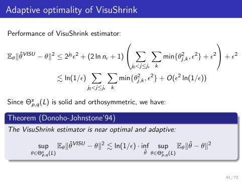
Adaptive optimality of VisuShrink

Performance of VisuShrink estimator:

Eθ‖θVISU − θ‖2 ≤ 2j0ε2 + (2 ln nε + 1)

∑j0<j≤jε

∑k

min{θ2j ,k , ε

2}+ ε2

+ ε2

. ln(1/ε)∑

j0<j≤jε

∑k

min{θ2j ,k , ε

2}+ O(ε2 ln(1/ε))

Since Θsp,q(L) is solid and orthosymmetric, we have:


The VisuShrink estimator is near optimal and adaptive:

supθ∈Θs

p,q(L)Eθ‖θVISU − θ‖2 . ln(1/ε) · inf

θsup

θ∈Θsp,q(L)

Eθ‖θ − θ‖2

41 / 72

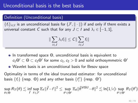
Unconditional basis is the best basis

Definition (Unconditional basis)

{fi}i∈I is an unconditional basis for (F , ‖ · ‖) if and only if there exists auniversal constant C such that for any J ⊂ I and λi ∈ [−1, 1],

‖∑i∈J

λi fi‖ ≤ C‖∑i∈J

fi‖

In transformed space Θ, unconditional basis is equivalent toc1Θ′ ⊂ Θ ⊂ c2Θ′ for some c1, c2 > 0 and solid orthosymmetric Θ′

Wavelet basis is an unconditional basis for Besov space

Optimality in terms of the ideal truncated estimator: for unconditionalbasis {fi} (resp. Θ) and any other basis {f ′i } (resp. Θ′)

supθ∈Θ

RT (θ) . inff

supf ∈F

Ef ‖f−f ‖2 ≤ supθ′∈Θ′

Eθ‖θVISU−θ‖2 . ln(1/ε)· supθ′∈Θ′

RT (θ′)

42 / 72

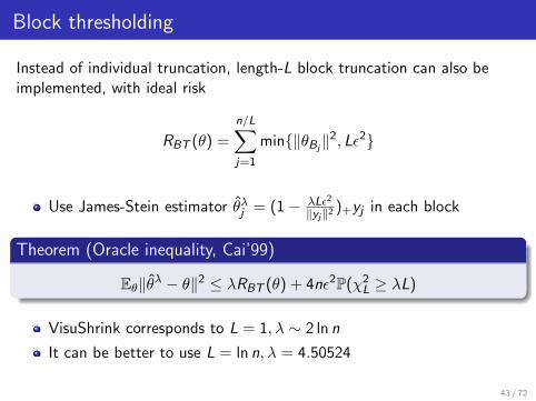
Block thresholding

Instead of individual truncation, length-L block truncation can also beimplemented, with ideal risk

RBT (θ) =

n/L∑j=1

min{‖θBj‖2, Lε2}

Use James-Stein estimator θλj = (1− λLε2

‖yj‖2 )+yj in each block

Theorem (Oracle inequality, Cai’99)

Eθ‖θλ − θ‖2 ≤ λRBT (θ) + 4nε2P(χ2L ≥ λL)

VisuShrink corresponds to L = 1, λ ∼ 2 ln n

It can be better to use L = ln n, λ = 4.50524

43 / 72




4 Miscellaneous

44 / 72

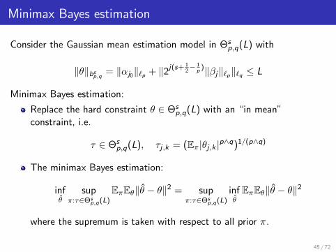
Minimax Bayes estimation

Consider the Gaussian mean estimation model in Θsp,q(L) with

‖θ‖bsp,q = ‖αj0‖`p + ‖2j(s+ 12− 1

p)‖βj‖`p‖`q ≤ L

Minimax Bayes estimation:

Replace the hard constraint θ ∈ Θsp,q(L) with an “in mean”

constraint, i.e.

τ ∈ Θsp,q(L), τj ,k = (Eπ|θj ,k |p∧q)1/(p∧q)

The minimax Bayes estimation:

infθ

supπ:τ∈Θs

p,q(L)EπEθ‖θ − θ‖2 = sup

π:τ∈Θsp,q(L)

infθEπEθ‖θ − θ‖2

where the supremum is taken with respect to all prior π.

45 / 72

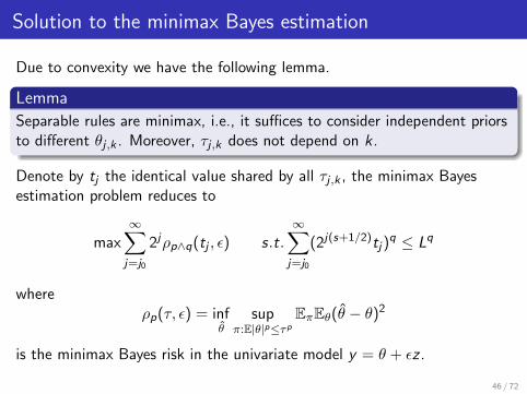
Solution to the minimax Bayes estimation

Due to convexity we have the following lemma.

Lemma

Separable rules are minimax, i.e., it suffices to consider independent priorsto different θj ,k . Moreover, τj ,k does not depend on k.

Denote by tj the identical value shared by all τj ,k , the minimax Bayesestimation problem reduces to

max∞∑j=j0

2jρp∧q(tj , ε) s.t.∞∑j=j0

(2j(s+1/2)tj)q ≤ Lq

whereρp(τ, ε) = inf

θsup

π:E|θ|p≤τpEπEθ(θ − θ)2

is the minimax Bayes risk in the univariate model y = θ + εz .

46 / 72

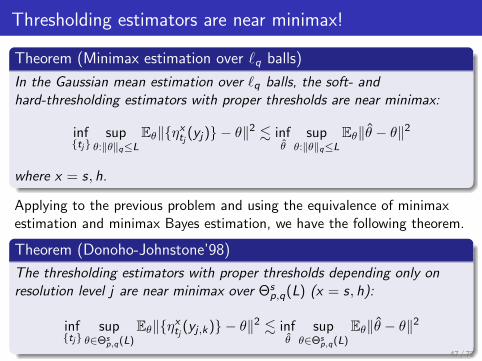
Thresholding estimators are near minimax!

Theorem (Minimax estimation over `q balls)

In the Gaussian mean estimation over `q balls, the soft- andhard-thresholding estimators with proper thresholds are near minimax:

inf{tj}

supθ:‖θ‖q≤L

Eθ‖{ηxtj (yj)} − θ‖2 . inf

θsup

θ:‖θ‖q≤LEθ‖θ − θ‖2

where x = s, h.

Applying to the previous problem and using the equivalence of minimaxestimation and minimax Bayes estimation, we have the following theorem.


The thresholding estimators with proper thresholds depending only onresolution level j are near minimax over Θs

p,q(L) (x = s, h):

inf{tj}

supθ∈Θs

p,q(L)Eθ‖{ηxtj (yj ,k)} − θ‖2 . inf

θsup

θ∈Θsp,q(L)

Eθ‖θ − θ‖2

47 / 72

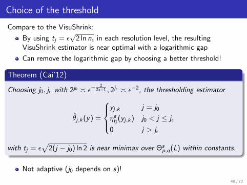
Choice of the threshold

Compare to the VisuShrink:

By using tj = ε√

2 ln nε in each resolution level, the resultingVisuShrink estimator is near optimal with a logarithmic gap

Can remove the logarithmic gap by choosing a better threshold!

Theorem (Cai’12)

Choosing j0, jε with 2j0 � ε−2

2s+1 , 2jε � ε−2, the thresholding estimator

θj ,k(y) =

yj ,k j = j0

ηstj (yj ,k) j0 < j ≤ jε

0 j > jε

with tj = ε√

2(j − j0) ln 2 is near minimax over Θsp,q(L) within constants.

Not adaptive (j0 depends on s)!

48 / 72

SURE: Stein’s unbiased risk estimator

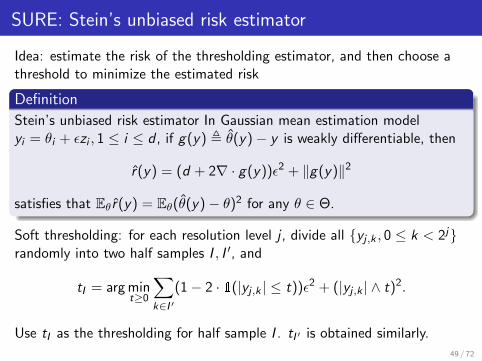
Idea: estimate the risk of the thresholding estimator, and then choose athreshold to minimize the estimated risk

Definition

Stein’s unbiased risk estimator In Gaussian mean estimation modelyi = θi + εzi , 1 ≤ i ≤ d , if g(y) , θ(y)− y is weakly differentiable, then

r(y) = (d + 2∇ · g(y))ε2 + ‖g(y)‖2

satisfies that Eθ r(y) = Eθ(θ(y)− θ)2 for any θ ∈ Θ.

Soft thresholding: for each resolution level j , divide all {yj ,k , 0 ≤ k < 2j}randomly into two half samples I , I ′, and

tI = arg mint≥0

∑k∈I ′

(1− 2 · 1(|yj ,k | ≤ t))ε2 + (|yj ,k | ∧ t)2.

Use tI as the thresholding for half sample I . tI ′ is obtained similarly.

49 / 72

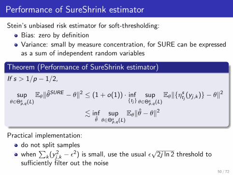
Performance of SureShrink estimator

Stein’s unbiased risk estimator for soft-thresholding:

Bias: zero by definition

Variance: small by measure concentration, for SURE can be expressedas a sum of independent random variables

Theorem (Performance of SureShrink estimator)

If s > 1/p − 1/2,

supθ∈Θs

p,q(L)Eθ‖θSURE − θ‖2 ≤ (1 + o(1)) · inf

{tj}sup

θ∈Θsp,q(L)

Eθ‖{ηstj (yj ,k)} − θ‖2

. infθ

supθ∈Θs

p,q(L)Eθ‖θ − θ‖2

Practical implementation:

do not split samples

when∑

k(y2j ,k − ε2) is small, use the usual ε

√2j ln 2 threshold to

sufficiently filter out the noise50 / 72

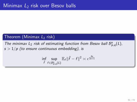
Minimax L2 risk over Besov balls

Theorem (Minimax L2 risk)

The minimax L2 risk of estimating function from Besov ball Bsp,q(L),s > 1/p (to ensure continuous embedding), is

inff

supf ∈Bsp,q(L)

Ef ‖f − f ‖2 � ε4s

2s+1

51 / 72

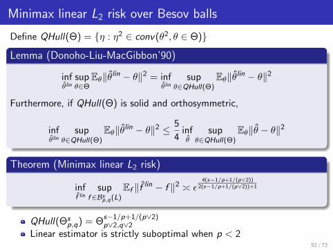
Minimax linear L2 risk over Besov balls

Define QHull(Θ) = {η : η2 ∈ conv(θ2, θ ∈ Θ)}

Lemma (Donoho-Liu-MacGibbon’90)

infθlin

supθ∈Θ

Eθ‖θlin − θ‖2 = infθlin

supθ∈QHull(Θ)

Eθ‖θlin − θ‖2

Furthermore, if QHull(Θ) is solid and orthosymmetric,

infθlin

supθ∈QHull(Θ)

Eθ‖θlin − θ‖2 ≤ 5

4infθ

supθ∈QHull(Θ)

Eθ‖θ − θ‖2

Theorem (Minimax linear L2 risk)

inff lin

supf ∈Bsp,q(L)

Ef ‖f lin − f ‖2 � ε4(s−1/p+1/(p∨2))

2(s−1/p+1/(p∨2))+1

QHull(Θsp,q) = Θ

s−1/p+1/(p∨2)p∨2,q∨2

Linear estimator is strictly suboptimal when p < 252 / 72




4 Miscellaneous

53 / 72

Estimation with Lr risk

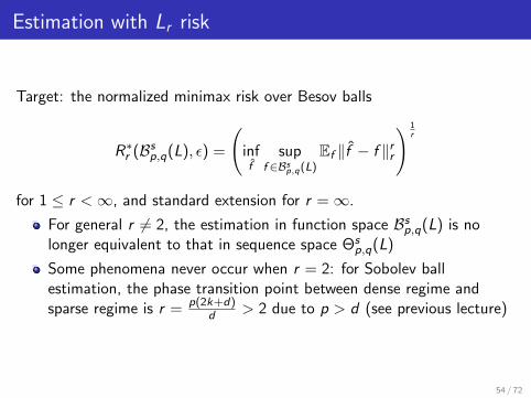
Target: the normalized minimax risk over Besov balls

R∗r (Bsp,q(L), ε) =

(inff

supf ∈Bsp,q(L)

Ef ‖f − f ‖rr

) 1r

for 1 ≤ r <∞, and standard extension for r =∞.

For general r 6= 2, the estimation in function space Bsp,q(L) is nolonger equivalent to that in sequence space Θs

p,q(L)

Some phenomena never occur when r = 2: for Sobolev ballestimation, the phase transition point between dense regime andsparse regime is r = p(2k+d)

d > 2 due to p > d (see previous lecture)

54 / 72

Minimax Lr risk

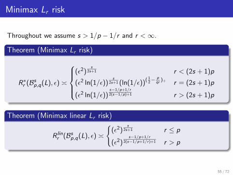
Throughout we assume s > 1/p − 1/r and r <∞.

Theorem (Minimax Lr risk)

R∗r (Bsp,q(L), ε) �

(ε2)

s2s+1 r < (2s + 1)p

(ε2 ln(1/ε))s

2s+1 (ln(1/ε))( 12− p

qr)+ r = (2s + 1)p

(ε2 ln(1/ε))s−1/p+1/r2(s−1/p)+1 r > (2s + 1)p

Theorem (Minimax linear Lr risk)

R linr (Bsp,q(L), ε) �

{(ε2)

s2s+1 r ≤ p

(ε2)s−1/p+1/r

2(s−1/p+1/r)+1 r > p

55 / 72

Three different zones

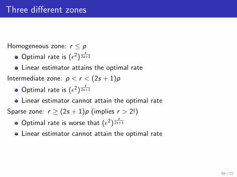
Homogeneous zone: r ≤ p

Optimal rate is (ε2)s

2s+1

Linear estimator attains the optimal rate

Intermediate zone: p < r < (2s + 1)p

Optimal rate is (ε2)s

2s+1

Linear estimator cannot attain the optimal rate

Sparse zone: r ≥ (2s + 1)p (implies r > 2!)

Optimal rate is worse that (ε2)s

2s+1

Linear estimator cannot attain the optimal rate

56 / 72

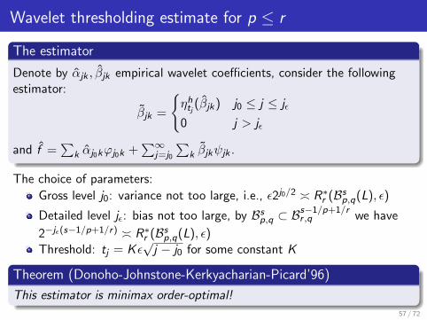
Wavelet thresholding estimate for p ≤ r

The estimator

Denote by αjk , βjk empirical wavelet coefficients, consider the followingestimator:

βjk =

{ηhtj (βjk) j0 ≤ j ≤ jε

0 j > jε

and f =∑

k αj0kϕj0k +∑∞

j=j0

∑k βjkψjk .

The choice of parameters:

Gross level j0: variance not too large, i.e., ε2j0/2 � R∗r (Bsp,q(L), ε)

Detailed level jε: bias not too large, by Bsp,q ⊂ Bs−1/p+1/rr ,q we have

2−jε(s−1/p+1/r) � R∗r (Bsp,q(L), ε)Threshold: tj = Kε

√j − j0 for some constant K

Theorem (Donoho-Johnstone-Kerkyacharian-Picard’96)

This estimator is minimax order-optimal!

57 / 72

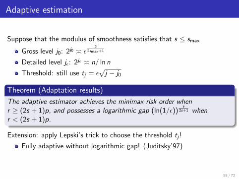
Adaptive estimation

Suppose that the modulus of smoothness satisfies that s ≤ smax

Gross level j0: 2j0 � ε2

2smax+1

Detailed level jε: 2jε � n/ ln n

Threshold: still use tj = ε√j − j0

Theorem (Adaptation results)

The adaptive estimator achieves the minimax risk order whenr ≥ (2s + 1)p, and possesses a logarithmic gap (ln(1/ε))

s2s+1 when

r < (2s + 1)p.

Extension: apply Lepski’s trick to choose the threshold tj !

Fully adaptive without logarithmic gap! (Juditsky’97)

58 / 72




4 Miscellaneous

59 / 72

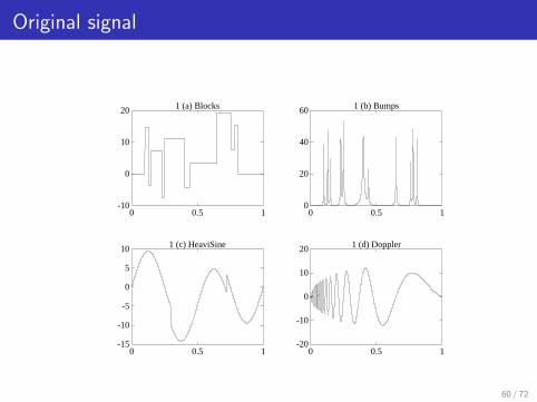
Original signal

-10

0

10

20

0 0.5 1

1 (a) Blocks

0

20

40

60

0 0.5 1

1 (b) Bumps

-15

-10

-5

0

5

10

0 0.5 1

1 (c) HeaviSine

-20

-10

0

10

20

0 0.5 1

1 (d) Doppler

60 / 72

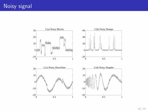
Noisy signal

-10

0

10

20

30

0 0.5 1

3 (a) Noisy Blocks

-20

0

20

40

60

0 0.5 1

3 (b) Noisy Bumps

-20

-10

0

10

20

0 0.5 1

3 (c) Noisy HeaviSine

-20

-10

0

10

20

0 0.5 1

3 (d) Noisy Doppler

61 / 72

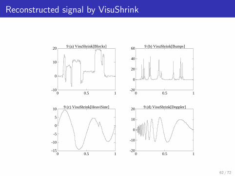
Reconstructed signal by VisuShrink

-10

0

10

20

0 0.5 1

9 (a) VisuShrink[Blocks]

-20

0

20

40

60

0 0.5 1

9 (b) VisuShrink[Bumps]

-15

-10

-5

0

5

10

0 0.5 1

9 (c) VisuShrink[HeaviSine]

-20

-10

0

10

20

0 0.5 1

9 (d) VisuShrink[Doppler]

62 / 72

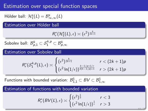
Estimation over special function spaces

Holder ball: Hs1(L) = Bs∞,∞(L)

Estimation over Holder ball

R∗r (Hs1(L), ε) � (ε2)

s2s+1

Sobolev ball: Bkp,1 ⊂ Sk,p1 ⊂ Bkp,∞

Estimation over Sobolev ball

R∗r (Sk,p1 (L), ε) �

(ε2)k

2k+1 r < (2k + 1)p

(ε2 ln(1/ε))k−1/p+1/r2(k−1/p)+1 r > (2k + 1)p

Functions with bounded variation: B11,1 ⊂ BV ⊂ B1

1,∞

Estimation of functions with bounded variation

R∗r (BV (L), ε) �

{(ε2)

13 r < 3

(ε2 ln(1/ε))1r r > 3

63 / 72

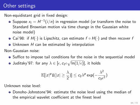
Other settings

Non-equidistant grid in fixed design:

Suppose xi = H−1(i/n) in regression model (or transform the noise toStandard Brownian motion via time change in the Gaussian whitenoise model)

Cai’98: if H(·) is Lipschitz, can estimate f ◦ H(·) and then recover f

Unknown H can be estimated by interpolation

Non-Gaussian noise:

Suffice to impose tail conditions for the noise in the sequential model

Juditsky’97: for any λ ∈ [ε, c1ε√

ln(1/ε)], it holds

E[|z |p1(|z | ≥ λ

2)] ≤ c2λ

p exp(− λ2

c3ε2)

Unknown noise level:

Donoho-Johnstone’94: estimate the noise level using the median ofthe empirical wavelet coefficient at the finest level

64 / 72

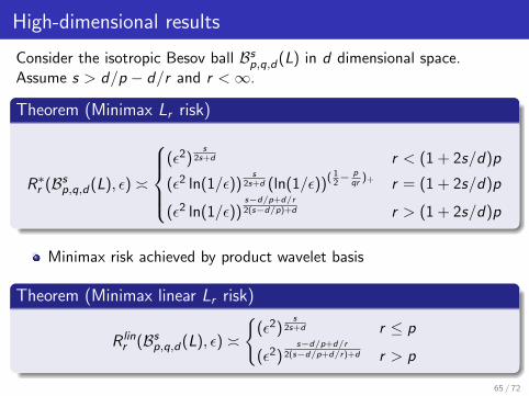
High-dimensional results

Consider the isotropic Besov ball Bsp,q,d(L) in d dimensional space.Assume s > d/p − d/r and r <∞.

Theorem (Minimax Lr risk)

R∗r (Bsp,q,d(L), ε) �

(ε2)

s2s+d r < (1 + 2s/d)p

(ε2 ln(1/ε))s

2s+d (ln(1/ε))( 12− p

qr)+ r = (1 + 2s/d)p

(ε2 ln(1/ε))s−d/p+d/r2(s−d/p)+d r > (1 + 2s/d)p

Minimax risk achieved by product wavelet basis

Theorem (Minimax linear Lr risk)

R linr (Bsp,q,d(L), ε) �

{(ε2)

s2s+d r ≤ p

(ε2)s−d/p+d/r

2(s−d/p+d/r)+d r > p

65 / 72

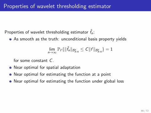
Properties of wavelet thresholding estimator

Properties of wavelet thresholding estimator fn:

As smooth as the truth: unconditional basis property yields

limn→∞

Pf {‖fn‖Bsp,q ≤ C‖f ‖Bsp,q} = 1

for some constant C .

Near optimal for spatial adaptation

Near optimal for estimating the function at a point

Near optimal for estimating the function under global loss

66 / 72

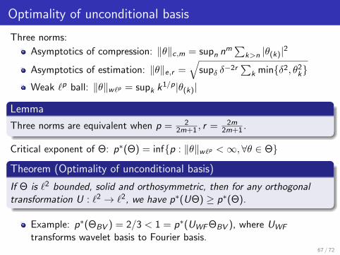
Optimality of unconditional basis

Three norms:

Asymptotics of compression: ‖θ‖c,m = supn nm∑

k>n |θ(k)|2

Asymptotics of estimation: ‖θ‖e,r =√

supδ δ−2r∑

k min{δ2, θ2k}

Weak `p ball: ‖θ‖w`p = supk k1/p|θ(k)|

Lemma

Three norms are equivalent when p = 22m+1 , r = 2m

2m+1 .

Critical exponent of Θ: p∗(Θ) = inf{p : ‖θ‖w`p <∞, ∀θ ∈ Θ}

Theorem (Optimality of unconditional basis)

If Θ is `2 bounded, solid and orthosymmetric, then for any orthogonaltransformation U : `2 → `2, we have p∗(UΘ) ≥ p∗(Θ).

Example: p∗(ΘBV ) = 2/3 < 1 = p∗(UWFΘBV ), where UWF

transforms wavelet basis to Fourier basis.67 / 72

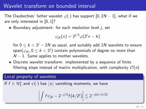
Wavelet transform on bounded interval

The Daubechies’ father wavelet ϕ(·) has support [0, 2N − 1], what if weare only interested in [0, 1]?

Boundary adjustment: for each resolution level j , set

ϕjk(x) = 2j/2ϕ(2jx − k)

for 0 ≤ k < 2j − 2N as usual, and suitably add 2N wavelets to ensurespan(ϕjk , 0 ≤ k < 2j) contain polynomials of degree no more thanN − 1. Same applies to mother wavelets.

Discrete wavelet transform: implemented by a sequence of finitefiltering steps instead of matrix multiplication, with complexity O(n)

Local property of wavelets

If f ∈ Hs1 and ψ(·) has bsc vanishing moments, we have∣∣∣∣∫ f ψjk − 2−j/2f (k/2j)

∣∣∣∣ . 2−j(s+1/2)

68 / 72

Multiresolution analysis

Asymptotic equivalence of models under mild conditions:

Gaussian white noise model:

dYt = f (t)dt +σ√ndBt , t ∈ [0, 1]

Density estimation model: generate n iid samples from commondensity g with support [0, 1] (g = f 2, σ = 1/2)

Proof depends heavily on multiresolution analysis (see Brown et al’04)!

69 / 72

General modulus of smoothness

Definition (Ditzian-Totik modulus of smoothness)

ωrϕ(f , t)p = sup

0<h≤t‖∆r

hϕ(x)f ‖p

Trigonometric approximation on [0, 1] (ϕ ≡ 1):

Denote by ETn (f )p the best approximation error in Lp norm using

trigonometric series of degree no more than n

Direct inequality: ETn (f )p ≤ Cr ,1ω

r (f , n−1)p

Converse: ωr (f , n−1)p ≤ Cr ,2n−r ∑n

k=1 kr−1ET

k (f )p

Polynomial approximation on [0, 1] (ϕ =√x(1− x)):

Denote by En(f )p the best approximation error in Lp norm usingalgebraic polynomials of degree no more than n

Direct inequality: En(f )p ≤ Dr ,1ωrϕ(f , n−1)p

Converse: ωrϕ(f , n−1)p ≤ Dr ,2n

−r ∑nk=1 k

r−1Ek(f )p

70 / 72

General K-functionals

Definition (General K-functional)

The general K-functional Kr ,ϕ(f , t)p is defined as

Kr ,ϕ(f , t)p = infg (r−1)∈A.C.loc

‖f − g‖p + t‖ϕrg (r)‖p

Theorem (Equivalence of K-functional and modulus of smoothness)

Under mild conditions on ϕ, we have

ωrϕ(f , t)p � Kr ,ϕ(f , tr )p

Bias analysis of plug-in estimator: for np ∼ B(n, p) and any f ,

|Epf (p)− f (p)| ≤ infg∈C2

|Epg(p)− g(p)|+ 2‖f − g‖∞

. infg∈C2

n−1‖p(1− p)g ′′(p)‖∞ + ‖f − g‖∞ . ω2ϕ(f , n−1/2)∞

where ϕ(x) =√

x(1− x).71 / 72

References

Nonparametric regression:

A series of paper by Donoho, Johnstone, etc. in 1990s.

I. Johnstone. Gaussian estimation: sequence and wavelet models.Manuscript (available online athttp://statweb.stanford.edu/~imj/GE06-11-13.pdf), 2013.

Approximation theory:

R. A. DeVore and G. G. Lorentz, Constructive approximation.Springer Science & Business Media, 1993.

Z. Ditzian and V. Totik, Moduli of smoothness. Vol. 9. SpringerScience & Business Media, 2012.

Wavelet and Besov space:

W. Hardle, G. Kerkyacharian, D. Picard, and A. Tsybakov. Wavelets,approximation, and statistical applications. Vol. 129. SpringerScience & Business Media, 2012.

72 / 72

http://statweb.stanford.edu/~imj/GE06-11-13.pdf

nonparametric estimation: part ii - stanford universityyjhan/nonparametric... · nonparametric...

Documents