nonparametric predictive inference for multiple...
TRANSCRIPT
Nonparametric Predictive Inference
for Multiple Comparisons
Tahani A. Maturi
A thesis presented for the degree of
Doctor of Philosophy
Department of Mathematical Sciences
Durham University
UK
May 2010

DedicatedTo my mother for her unlimited love and care
Nonparametric Predictive Inference for Multiple
Comparisons
Tahani A. Maturi
Submitted for the degree of Doctor of Philosophy
May 2010
Abstract
This thesis presents Nonparametric Predictive Inference (NPI) for several multiple
comparisons problems. We introduce NPI for comparison of multiple groups of data
including right-censored observations. Different right-censoring schemes discussed
are early termination of an experiment, progressive censoring and competing risks.
Several selection events of interest are considered including selecting the best group,
the subset of best groups, and the subset including the best group. The proposed
methods use lower and upper probabilities for some events of interest formulated
in terms of the next future observation per group. For each of these problems the
required assumptions are Hill’s assumption A(n) and the generalized assumption
rc-A(n) for right-censored data.
Attention is also given to the situation where only a part of the data range is
considered relevant for the inference, where in addition the numbers of observations
to the left and to the right of this range are known. Throughout this thesis, our
methods are illustrated and discussed via examples with data from the literature.

Declaration
The work in this thesis is based on research carried out at the Department of Mathe-
matical Sciences, Durham University, UK. No part of this thesis has been submitted
elsewhere for any other degree or qualification and it is all the author’s original work
unless referenced to the contrary in the text.
Copyright c© 2010 by Tahani A. Maturi.
The copyright of this thesis rests with the author. No quotations from it should be
published without the author’s prior written consent and information derived from
it should be acknowledged.
iv

Acknowledgements
My main appreciation and thanks go to my first supervisor Dr. Pauline Coolen-
Schrijner. To my great sadness, Pauline passed away on 23 April 2008 due to her
illness. She was a very supportive and nice person, who helped me greatly during
my study, which will have significant impact on my future career. I hope she is
proud of this thesis.
My special thanks go to my second supervisor Prof. Frank Coolen for his unlim-
ited support, expert advice and guidance.
Mathematics is not a subject to me; it is my love in life. This is because of my
lovely mother who taught me mathematics from an early age when mathematics was
my reward for learning the alphabet. Without my mother and her prayer I would
not be at this stage of my career in mathematics.
I am immensely grateful to my parents, my brothers (especially Hani who came
along with me to the UK), my lovely sister Amani and my dearest cousin Dalal for
their invaluable care, support and encouragement.
My final thanks go to King Abdulaziz University, Jeddah, Saudi Arabia, for
offering me the opportunity to complete my studies abroad.
v
Contents
Abstract iii
Declaration iv
Acknowledgements v
1 Introduction 1
1.1 Overview . . . . . . . . . . . . . . . . . . . . . . . . . . . . . . . . . . 1
1.2 Assumption A(n) and imprecise probability . . . . . . . . . . . . . . . 2
1.3 Nonparametric Predictive Inference (NPI) . . . . . . . . . . . . . . . 3
1.3.1 NPI for multiple comparisons . . . . . . . . . . . . . . . . . . 5
1.3.2 NPI for right-censored data . . . . . . . . . . . . . . . . . . . 7
1.3.3 NPI for survival function . . . . . . . . . . . . . . . . . . . . . 10
1.3.4 NPI for comparing two groups of lifetime data . . . . . . . . . 13
1.3.5 Treatment of ties . . . . . . . . . . . . . . . . . . . . . . . . . 14
1.4 Outline of Thesis . . . . . . . . . . . . . . . . . . . . . . . . . . . . . 14
2 Comparison of two groups with early termination 16
2.1 Introduction . . . . . . . . . . . . . . . . . . . . . . . . . . . . . . . . 16
2.2 Classical precedence testing . . . . . . . . . . . . . . . . . . . . . . . 17
2.3 NPI for precedence testing . . . . . . . . . . . . . . . . . . . . . . . . 19
2.4 NPI for comparing two groups with early termination . . . . . . . . . 21
2.4.1 Special cases . . . . . . . . . . . . . . . . . . . . . . . . . . . . 23
2.4.2 Some properties . . . . . . . . . . . . . . . . . . . . . . . . . . 24
2.5 Examples . . . . . . . . . . . . . . . . . . . . . . . . . . . . . . . . . 26
vi
Contents vii
2.6 Concluding remarks . . . . . . . . . . . . . . . . . . . . . . . . . . . . 30
3 Multiple comparisons with early termination 32
3.1 Introduction . . . . . . . . . . . . . . . . . . . . . . . . . . . . . . . . 32
3.2 Classical methods . . . . . . . . . . . . . . . . . . . . . . . . . . . . . 32
3.3 Selecting the best group . . . . . . . . . . . . . . . . . . . . . . . . . 35
3.3.1 Special cases . . . . . . . . . . . . . . . . . . . . . . . . . . . . 36
3.3.2 Some properties . . . . . . . . . . . . . . . . . . . . . . . . . . 38
3.4 Selecting the subset of best groups . . . . . . . . . . . . . . . . . . . 46
3.4.1 Special cases . . . . . . . . . . . . . . . . . . . . . . . . . . . . 48
3.4.2 Some properties . . . . . . . . . . . . . . . . . . . . . . . . . . 49
3.5 Selecting the subset including the best group . . . . . . . . . . . . . . 56
3.5.1 Special cases . . . . . . . . . . . . . . . . . . . . . . . . . . . . 56
3.5.2 Some properties . . . . . . . . . . . . . . . . . . . . . . . . . . 57
3.6 Concluding remarks . . . . . . . . . . . . . . . . . . . . . . . . . . . . 68
4 Comparisons of lifetime data with early termination 69
4.1 Introduction . . . . . . . . . . . . . . . . . . . . . . . . . . . . . . . . 69
4.2 Classical precedence tests . . . . . . . . . . . . . . . . . . . . . . . . 70
4.3 NPI for lifetime data with early termination . . . . . . . . . . . . . . 71
4.4 Examples . . . . . . . . . . . . . . . . . . . . . . . . . . . . . . . . . 76
4.5 Concluding remarks . . . . . . . . . . . . . . . . . . . . . . . . . . . . 80
5 Progressive Censoring 82
5.1 Introduction . . . . . . . . . . . . . . . . . . . . . . . . . . . . . . . . 82
5.2 Progressive censoring schemes . . . . . . . . . . . . . . . . . . . . . . 83
5.3 NPI for progressive Type-II censoring . . . . . . . . . . . . . . . . . . 87
5.4 NPI for progressive Type-I censoring . . . . . . . . . . . . . . . . . . 91
5.5 NPI for Type-II progressively hybrid censoring . . . . . . . . . . . . . 92
5.6 Example . . . . . . . . . . . . . . . . . . . . . . . . . . . . . . . . . . 94
5.7 Concluding remarks . . . . . . . . . . . . . . . . . . . . . . . . . . . . 98
Contents viii
6 Competing Risks 99
6.1 Introduction . . . . . . . . . . . . . . . . . . . . . . . . . . . . . . . . 99
6.2 Competing risks . . . . . . . . . . . . . . . . . . . . . . . . . . . . . . 100
6.3 NPI for Competing Risks . . . . . . . . . . . . . . . . . . . . . . . . . 101
6.4 Two competing risks . . . . . . . . . . . . . . . . . . . . . . . . . . . 104
6.5 Examples . . . . . . . . . . . . . . . . . . . . . . . . . . . . . . . . . 108
6.6 Progressive Type-II censoring . . . . . . . . . . . . . . . . . . . . . . 117
6.7 Concluding remarks . . . . . . . . . . . . . . . . . . . . . . . . . . . . 120
7 Comparison with terminated tails 121
7.1 Introduction . . . . . . . . . . . . . . . . . . . . . . . . . . . . . . . . 121
7.2 Classical methods . . . . . . . . . . . . . . . . . . . . . . . . . . . . 122
7.3 NPI with terminated tails . . . . . . . . . . . . . . . . . . . . . . . . 124
7.4 Comparing two groups with terminated tails . . . . . . . . . . . . . . 126
7.5 Special cases . . . . . . . . . . . . . . . . . . . . . . . . . . . . . . . . 129
7.6 Example . . . . . . . . . . . . . . . . . . . . . . . . . . . . . . . . . . 132
7.7 Concluding remarks . . . . . . . . . . . . . . . . . . . . . . . . . . . . 136
8 Conclusions 138
Appendix 141
A An illustrative example of rc-A(n) 141
B R programs 144
B.1 NPI for multiple comparison of lifetime data . . . . . . . . . . . . . . 144
B.2 NPI for comparing two groups with terminated tails . . . . . . . . . 149
Bibliography 151
Chapter 1
Introduction
1.1 Overview
This thesis presents Nonparametric Predictive Inference (NPI) for several compar-
isons problems. Mainly, we introduce NPI for multiple comparisons in situations
with right-censored observations. Such data typically occur in reliability or survival
analysis, due to several reasons. For example, when interest is in a specific failure
mode for a technical unit, it may fail due to a different failure cause. If multiple
failure modes are of interest, and failure will be due to only a single failure mode,
then this situation is known as ’competing risks’, where an observed failure time is
actually a right-censoring time with regard to all failure modes that did not cause
the failure. Another reason for right-censoring may be removal of units from a life-
time experiment, normally to save time or reduce costs, but this also occurs if, at
some point, one wishes to study in more detail units which have not yet failed in
an experiment. If right-censoring is due to an experiment being terminated before
all units have failed, comparison of different groups of units based on such data is
known as ’precedence testing’. If non-failing units are removed from the experiment
at several possible stages it is known as ’progressive censoring’.
In this thesis, we develop NPI for multiple comparisons for precedence testing,
progressive censoring, and competing risks. It should be emphasized that, through-
out the thesis, unspecified reasons for right-censoring are assumed to be based on
processes that are independent of the residual lifetimes of the censored units. We
1
1.2. Assumption A(n) and imprecise probability 2
also present NPI for situations where the information available consists of precise
measurements of real-valued data only within a specific range, with in addition the
numbers of observations to the left and to the right of this range are known.
Section 1.2 provides a brief overview of some basic aspects of imprecise probabil-
ity and the underlying assumption behind NPI, Hill’s assumption A(n). In Section
1.3 we review briefly the main idea of NPI and discuss some applications which
we will refer to later in the thesis. This includes the generalisation of the A(n) as-
sumption needed to accommodate lifetime data, the so-called assumption rc-A(n).
Finally, the outline of this thesis is given in Section 1.4.
1.2 Assumption A(n) and imprecise probability
In this section we briefly overview some basic aspects of imprecise probability and
the underlying assumption behind NPI, Hill’s assumption A(n) [40]. To introduce
A(n) we first need to introduce some notation. Suppose that X1, . . . , Xn, Xn+1 are
real-valued absolutely continuous and exchangeable random quantities. Let the
ordered observed values of X1, X2, . . . , Xn be denoted by x1 < x2 < . . . < xn, and
let x0 = −∞ and xn+1 = ∞ for ease of notation. We assume that no ties occur,
the results can be generalised to allow ties [42], see also Subsection 1.3.5. Based
on n observations, the assumption A(n) is that the probability that the next future
observation Xn+1 falls in the open interval Ij = (xj, xj+1) is 1/(n + 1), for each
j = 0, 1, . . . , n [40].
A(n) does not assume anything else, and can be considered to be a post-data
assumption related to exchangeability [31]. Hill [41] discusses A(n) in detail. A(n)
is not sufficient to derive precise probabilities for many events of interest, but it
provides bounds for probabilities via the ‘fundamental theorem of probability’ [31],
which are lower and upper probabilities in interval probability theory [76, 79].
Lower and upper probabilities generalise classical probabilities, and a lower (up-
per) probability for event A, denoted by P (A) (P (A)), can be interpreted in several
ways [21]: as supremum buying (infimum selling) price for a gamble on the event
A, or as the maximum lower (minimum upper) bound for the probability of A that
1.3. Nonparametric Predictive Inference (NPI) 3
follows from the assumptions made. Informally, P (A) (P (A)) can be considered to
reflect the evidence in favour of (against) event A.
Interval probabilities, also know as imprecise probabilities, have been suggested
in various areas of statistics. Recently increasing attention has been given to this
topic area resulting in a series of conferences and a project website (The Society
for Imprecise Probability: Theories and Applications - www.sipta.org). Walley [76,
77] extended the traditional subjective probability theory via buying and selling
prices for gambles, whereas Weichselberger [78, 79] generalised Kolmogorov’s axioms
without imposing an interpretation.
Below we briefly present some elements of theory of interval probability as rele-
vant to A(n)-based inference. According to Weichselberger [78, 79], an axiomization
of interval probability can be achieved by supplementing Kolmogorov’s axioms as
follows:
For a measurable space (Ω,A), a set function p(.) on A satisfying Kolmogorov’s
axioms is called a classical probability. Let K(Ω,A) be the set of all classical prob-
abilities on (Ω,A). A function [P (.);P (.)] on A is called an F-probability with
structure M, if
i) P : A → [P ;P ]|0 ≤ P ≤ P ≤ 1 and A 7→ [P (A);P (A)],
ii) M := p(.) ∈ K(Ω,A)| P (A) ≤ p(A) ≤ P (A), ∀A ∈ A 6= ∅,
iii) For all A ∈ A, infp(.)∈M
p(A) = P (A) and supp(.)∈M
p(A) = P (A).
For every F -probability, P (A) and P (A) are conjugated, i.e. P (A) = 1 − P (Ac),
where Ac is the complement of A.
1.3 Nonparametric Predictive Inference (NPI)
Inferences based on A(n) are predictive and nonparametric, and can be considered
suitable if there is hardly any knowledge about the random quantity of interest,
other than the n observations, or if one does not want to use such information,
e.g. to study effects of additional assumptions underlying other statistical methods.
Nonparametric Predictive Inference (NPI) is a statistical method based on Hill’s
1.3. Nonparametric Predictive Inference (NPI) 4
assumption A(n) [40], which gives direct probabilities for a future observable random
quantity, given observed values of related random quantities [1, 21]. NPI has been
developed in recent years, mainly by Frank Coolen and Pauline Coolen-Schrijner and
their collaborators and students, for different applications in statistics, reliability and
operational research.
In NPI uncertainty is quantified by lower and upper probabilities for events of in-
terest. Augustin and Coolen [1] introduced predictive lower and upper probabilities
based on A(n) as follows:
Let B be the Borel σ-field over R. For any element B ∈ B, lower probability
P (.) and upper probability P (.) for the event Xn+1 ∈ B, based on the intervals
Ij = (xj, xj+1) (j = 0, 1, . . . , n) created by n real-valued non-tied observations, and
the assumption A(n), are
P (Xn+1 ∈ B) =1
n+ 1|j : Ij ⊆ B|
P (Xn+1 ∈ B) =1
n+ 1|j : Ij ∩ B 6= ∅|
where |A| is the cardinality of a set A, i.e. the number of elements contained in A.
In other words, the lower probability P (Xn+1 ∈ B) is achieved by taking only prob-
ability mass into account that is necessarily within B, which is only the case for the
probability mass 1n+1
per interval Ij if this interval is completely contained within B.
The upper probability P (Xn+1 ∈ B) is achieved by taking all the probability mass
into account that could possibly be within B, which is the case for the probability
mass 1n+1
, per interval Ij, if the intersection of Ij and B is non-empty.
Augustin and Coolen [1] showed that these bounds fit nicely into the framework
of interval probability [78, 79]. They proved that, without adding any further as-
sumptions, these A(n)-based lower and upper probabilities are F -probability with
structure
M := p(.) ∈ K(R,B)| p(Xn+1 ∈ Ij) =1
n+ 1, ∀j = 0, 1, . . . , n.
By the nature of A(n), NPI is a frequentist statistical methodology [1, 40, 41],
which however can be interpreted in a way similar to Bayesian statistics [21, 42].
An important advantage over more established frequentist methods is that NPI does
1.3. Nonparametric Predictive Inference (NPI) 5
not depend on counterfactuals, that is data which were not actually observed but
could have been observed. For example, these are important in hypothesis testing,
which has led to a large literature on frequentist methods for related problems con-
sidering slightly varying experimental procedures. In NPI, as in Bayesian statistics,
the inferences only involve the actual data observed, although a warning is needed
about the fact that, quite obviously, to apply NPI one must be happy with the
exchangeability assumption on the data and future observation(s), which may be
non-trivial depending on the experimental set-up.
1.3.1 NPI for multiple comparisons
For complete data, Coolen [19] introduced NPI for comparing two independent
groups, say X and Y . In classical statistics these tend to be referred to as ’popula-
tions’. Throughout this thesis, we avoid the term ‘populations’ in NPI as we only
consider one future observation and do not make use of any population distribution,
even no assumptions about existence of such a distribution or about a meaningful
population are made. Suppose that X1, . . . , Xnx, Xnx+1 and Y1, . . . , Yny
, Yny+1 are
real-valued absolutely continuous and exchangeable random quantities from X and
Y , respectively. Let their ordered observed values be x1 < x2 < . . . < xnxand
y1 < y2 < . . . < yny, and let x0 = y0 = −∞ and xnx+1 = yny+1 = ∞. Again we
assume that no ties occur, the results can be generalised to allow ties [42].
Such comparisons focus on the next future observation from each group. The
NPI lower and upper probabilities for the event that a future observation, Xnx+1, of
group X is less than a future observation, Yny+1, of group Y (i.e. Xnx+1 < Yny+1),
based on nx and ny observations of group X and Y , and the assumptions A(nx) for
Xnx+1 and A(ny) for Yny+1, are
P (Xnx+1 < Yny+1) =1
(nx + 1)(ny + 1)
ny∑
j=1
nx∑
i=1
1xi < yj (1.1)
P (Xnx+1 < Yny+1) =1
(nx + 1)(ny + 1)
ny∑
j=1
nx∑
i=1
1xi < yj+ nx + ny + 1
(1.2)
where 1E is an indicator function which is equal to 1 if event E occurs and 0 else.
For these lower and upper probabilities the conjugacy property holds, that is for an
1.3. Nonparametric Predictive Inference (NPI) 6
event E and its complementary event Ec, P (E) = 1− P (Ec).
Throughout we assume that information on units from one group does not hold
any information about units from the other group, so Xnx+1 and Yny+1 are indepen-
dent and data from group X contain no information on Yny+1 and vice versa. We
call this ‘complete independence’ of the groups.
Coolen and van der Laan [25] extended this to compare k ≥ 2 groups with
different events of interest including selection of the best group, the subset of best
groups, and the subset that includes the best group.
Suppose we have k ≥ 2 groups and nj + 1 random quantities from group j,
denoted by Xj,ij where ij = 1, 2, . . . , nj , nj + 1, j = 1, 2, . . . , k, and let for each
group j (j = 1, 2, . . . , k) xj,1 < xj,2 < . . . < xj,njbe the ordered observed values and
xj,0 = −∞ and xj,nj+1 = ∞. The inference depends on Hill’s assumption A(nj) [40]
for each group j, as described before.
Coolen and van der Laan [25] presented the following NPI lower and upper prob-
abilities for the event that a specific Xl,nl+1 is the maximum for all next observations
Xj,nj+1, j = 1, . . . , k.
P
(
Xl,nl+1 = max1≤j≤k
Xj,nj+1
)
=1
k∏
j=1
(nj + 1)
nl∑
il=1
k∏
j=1
j 6=l
nj∑
ij=1
1xj,ij < xl,il
P
(
Xl,nl+1 = max1≤j≤k
Xj,nj+1
)
=1
k∏
j=1
(nj + 1)
nl∑
il=1
k∏
j=1
j 6=l
1 +
nj∑
ij=1
1xj,ij< xl,il
+1
nl + 1
They also considered selection of a subset of groups such that all the groups in
this subset are ’better’ than all not selected groups, that is the next observation
of each group in the subset is greater than the next observation of all groups not
in the subset. Let S = l1, l2, ..., lm be a subset of m groups (1 ≤ m ≤ k − 1)
from k independent groups and let NS be the complement set of S containing the
remaining k −m groups. Then the NPI lower and upper probabilities for the event
that the next observation of each group in S is greater than the next observation of
1.3. Nonparametric Predictive Inference (NPI) 7
each group in NS, i.e. minl∈S
Xl,nl+1 > maxj∈NS
Xj,nj+1, are [25]
P
(
minl∈S
Xl,nl+1 > maxj∈NS
Xj,nj+1
)
=1
k∏
j=1
(nj + 1)
nl∑∑∑∑∑∑
il=1
l∈S
∏
j∈NS
nj∑
ij=1
1xj,ij < minl∈S
xl,il
P
(
minl∈S
Xl,nl+1 > maxj∈NS
Xj,nj+1
)
=1
k∏
j=1
(nj + 1)
nl+1∑∑∑∑∑∑
il=1
l∈S
∏
j∈NS
1+
nj∑
ij=1
1xj,ij< minl∈S
xl,il
where the notation
bl∑∑∑∑∑∑
il=a
l∈S
is used for the m sums
bl1∑
il1=a
...
blm∑
ilm=a
.
Using the same definitions of subsets S and NS, we can also be interested in
selecting the subset S that contains the best group. Then the NPI lower and upper
probabilities for the event that the next observation from (at least) one of the se-
lected groups in S is greater than the next observation from each group in NS, i.e.
maxl∈S
Xl,nl+1 > maxj∈NS
Xj,nj+1, are [25]
P
(
maxl∈S
Xl,nl+1 > maxj∈NS
Xj,nj+1
)
=1
k∏
j=1
(nj + 1)
nl∑∑∑∑∑∑
il=0
l∈S
∏
j∈NS
nj∑
ij=1
1xj,ij < maxl∈S
xl,il
P
(
maxl∈S
Xl,nl+1 > maxj∈NS
Xj,nj+1
)
=1
k∏
j=1
(nj + 1)
nl+1∑∑∑∑∑∑
il=1
l∈S
∏
j∈NS
1+
nj∑
ij=1
1xj,ij<maxl∈S
xl,il
1.3.2 NPI for right-censored data
In reliability and survival analysis, data on event times, often called lifetime, are
often affected by right-censoring, where for a specific unit or individual it is only
known that the event has not yet taken place at a specific time. An observation
for a unit or an individual is said to be right-censored at c when its lifetime is only
known to be greater than c [48].
The assumption A(n) requires fully observed data, and cannot deal directly with
right-censored data. Coolen and Yan [27] presented a generalisation of A(n), called
right-censoring A(n) or rc-A(n), which is suitable for right-censored data. In compar-
ison to A(n), rc-A(n) uses the extra assumption that, at the moment of censoring,
1.3. Nonparametric Predictive Inference (NPI) 8
the residual lifetime of a right-censored unit is exchangeable with the residual life-
times of all other units that have not yet failed or been censored. Further details
of rc-A(n) are given in [27]. To formulate the required form of rc-A(n), we need no-
tation for probability mass assigned to intervals without further restrictions on the
spread within the intervals. Such a partial specification of a probability distribution
is called an M -function [27] which is given by the following definition.
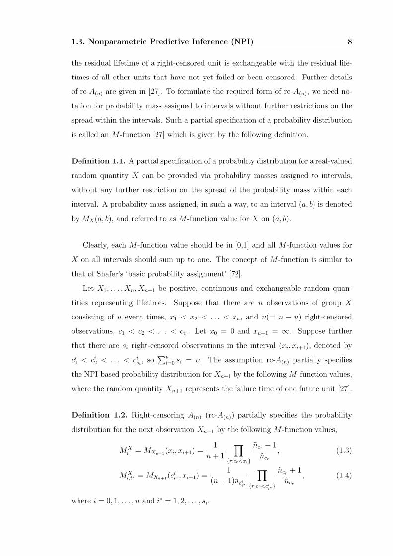
Definition 1.1. A partial specification of a probability distribution for a real-valued
random quantity X can be provided via probability masses assigned to intervals,
without any further restriction on the spread of the probability mass within each
interval. A probability mass assigned, in such a way, to an interval (a, b) is denoted
by MX(a, b), and referred to as M -function value for X on (a, b).
Clearly, each M -function value should be in [0,1] and all M -function values for
X on all intervals should sum up to one. The concept of M -function is similar to
that of Shafer’s ‘basic probability assignment’ [72].
Let X1, . . . , Xn, Xn+1 be positive, continuous and exchangeable random quan-
tities representing lifetimes. Suppose that there are n observations of group X
consisting of u event times, x1 < x2 < . . . < xu, and υ(= n − u) right-censored
observations, c1 < c2 < . . . < cυ. Let x0 = 0 and xu+1 = ∞. Suppose further
that there are si right-censored observations in the interval (xi, xi+1), denoted by
ci1 < ci2 < . . . < cisi , so∑u
i=0 si = υ. The assumption rc-A(n) partially specifies
the NPI-based probability distribution for Xn+1 by the following M -function values,
where the random quantity Xn+1 represents the failure time of one future unit [27].
Definition 1.2. Right-censoring A(n) (rc-A(n)) partially specifies the probability
distribution for the next observation Xn+1 by the following M -function values,
MXi = MXn+1(xi, xi+1) =
1
n+ 1
∏
r:cr<xi
ncr + 1
ncr
, (1.3)
MXi,i∗ = MXn+1(c
ii∗ , xi+1) =
1
(n+ 1)ncii∗
∏
r:cr<cii∗
ncr + 1
ncr
, (1.4)
where i = 0, 1, . . . , u and i∗ = 1, 2, . . . , si.
1.3. Nonparametric Predictive Inference (NPI) 9
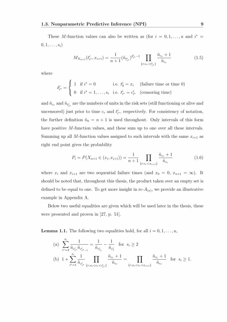
These M -function values can also be written as (for i = 0, 1, . . . , u and i∗ =
0, 1, . . . , si)
MXn+1(tii∗ , xi+1) =
1
n+ 1(nti
i∗)δ
ii∗−1
∏
r:cr<tii∗
ncr + 1
ncr
(1.5)
where
δii∗ =
1 if i∗ = 0 i.e. ti0 = xi (failure time or time 0)
0 if i∗ = 1, . . . , si i.e. tii∗ = cii∗ (censoring time)
and ncr and ntii∗are the numbers of units in the risk sets (still functioning or alive and
uncensored) just prior to time cr and tii∗ , respectively. For consistency of notation,
the further definition n0 = n + 1 is used throughout. Only intervals of this form
have positive M -function values, and these sum up to one over all these intervals.
Summing up all M -function values assigned to such intervals with the same xi+1 as
right end point gives the probability
Pi = P (Xn+1 ∈ (xi, xi+1)) =1
n+ 1
∏
r:cr<xi+1
ncr + 1
ncr
(1.6)
where xi and xi+1 are two sequential failure times (and x0 = 0, xu+1 = ∞). It
should be noted that, throughout this thesis, the product taken over an empty set is
defined to be equal to one. To get more insight in rc-A(n), we provide an illustrative
example in Appendix A.
Below two useful equalities are given which will be used later in the thesis, these
were presented and proven in [27, p. 51].
Lemma 1.1. The following two equalities hold, for all i = 0, 1, . . . , u,
(a)
si∑
i∗=2
1
ncii∗nci
i∗−1
=1
ncisi
− 1
nci1
for si ≥ 2
(b) 1 +
si∑
i∗=1
1
ncii∗
∏
r:xi<cr<cii∗
ncr + 1
ncr
=∏
r:xi<cr<xi+1
ncr + 1
ncr
for si ≥ 1.
1.3. Nonparametric Predictive Inference (NPI) 10
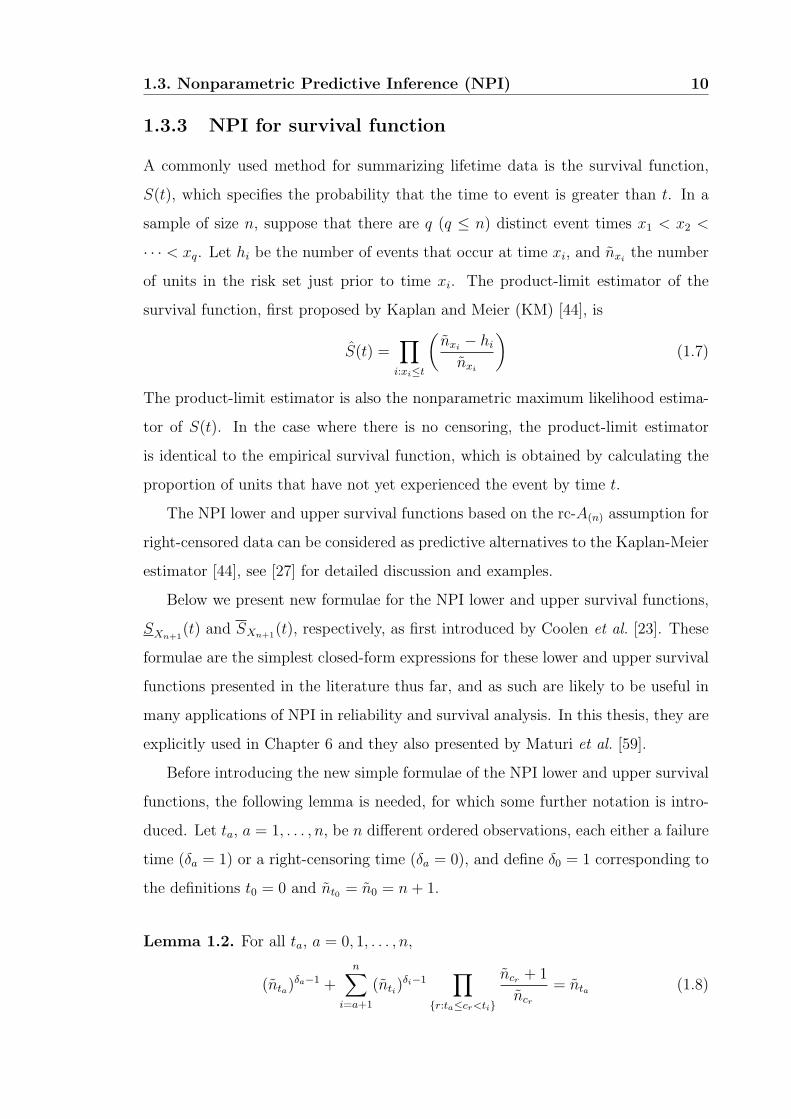
1.3.3 NPI for survival function
A commonly used method for summarizing lifetime data is the survival function,
S(t), which specifies the probability that the time to event is greater than t. In a
sample of size n, suppose that there are q (q ≤ n) distinct event times x1 < x2 <
· · · < xq. Let hi be the number of events that occur at time xi, and nxithe number
of units in the risk set just prior to time xi. The product-limit estimator of the
survival function, first proposed by Kaplan and Meier (KM) [44], is
S(t) =∏
i:xi≤t
(
nxi− hi
nxi
)
(1.7)
The product-limit estimator is also the nonparametric maximum likelihood estima-
tor of S(t). In the case where there is no censoring, the product-limit estimator
is identical to the empirical survival function, which is obtained by calculating the
proportion of units that have not yet experienced the event by time t.
The NPI lower and upper survival functions based on the rc-A(n) assumption for
right-censored data can be considered as predictive alternatives to the Kaplan-Meier
estimator [44], see [27] for detailed discussion and examples.
Below we present new formulae for the NPI lower and upper survival functions,
SXn+1(t) and SXn+1(t), respectively, as first introduced by Coolen et al. [23]. These
formulae are the simplest closed-form expressions for these lower and upper survival
functions presented in the literature thus far, and as such are likely to be useful in
many applications of NPI in reliability and survival analysis. In this thesis, they are
explicitly used in Chapter 6 and they also presented by Maturi et al. [59].
Before introducing the new simple formulae of the NPI lower and upper survival
functions, the following lemma is needed, for which some further notation is intro-
duced. Let ta, a = 1, . . . , n, be n different ordered observations, each either a failure
time (δa = 1) or a right-censoring time (δa = 0), and define δ0 = 1 corresponding to
the definitions t0 = 0 and nt0 = n0 = n+ 1.
Lemma 1.2. For all ta, a = 0, 1, . . . , n,
(nta)δa−1 +
n∑
i=a+1
(nti)δi−1
∏
r:ta≤cr<ti
ncr + 1
ncr
= nta (1.8)
1.3. Nonparametric Predictive Inference (NPI) 11
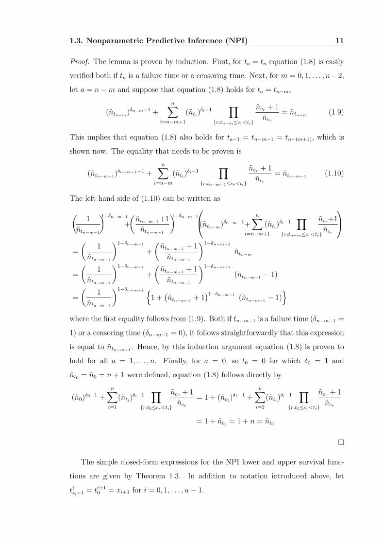
Proof. The lemma is proven by induction. First, for ta = tn equation (1.8) is easily
verified both if tn is a failure time or a censoring time. Next, for m = 0, 1, . . . , n−2,
let a = n−m and suppose that equation (1.8) holds for ta = tn−m,
(ntn−m)δn−m−1 +
n∑
i=n−m+1
(nti)δi−1
∏
r:tn−m≤cr<ti
ncr + 1
ncr
= ntn−m(1.9)
This implies that equation (1.8) also holds for ta−1 = tn−m−1 = tn−(m+1), which is
shown now. The equality that needs to be proven is
(ntn−m−1)δn−m−1−1 +
n∑
i=n−m
(nti)δi−1
∏
r:tn−m−1≤cr<ti
ncr + 1
ncr
= ntn−m−1 (1.10)
The left hand side of (1.10) can be written as
(
1
ntn−m−1
)1−δn−m−1
+
(
ntn−m−1+1
ntn−m−1
)1−δn−m−1
(ntn−m)δn−m−1+
n∑
i=n−m+1
(nti)δi−1
∏
r:tn−m≤cr<ti
ncr+1
ncr
=
(
1
ntn−m−1
)1−δn−m−1
+
(
ntn−m−1 + 1
ntn−m−1
)1−δn−m−1
ntn−m
=
(
1
ntn−m−1
)1−δn−m−1
+
(
ntn−m−1 + 1
ntn−m−1
)1−δn−m−1
(ntn−m−1 − 1)
=
(
1
ntn−m−1
)1−δn−m−1
1 +(
ntn−m−1 + 1)1−δn−m−1 (ntn−m−1 − 1)
where the first equality follows from (1.9). Both if tn−m−1 is a failure time (δn−m−1 =
1) or a censoring time (δn−m−1 = 0), it follows straightforwardly that this expression
is equal to ntn−m−1 . Hence, by this induction argument equation (1.8) is proven to
hold for all a = 1, . . . , n. Finally, for a = 0, so t0 = 0 for which δ0 = 1 and
nt0 = n0 = n+ 1 were defined, equation (1.8) follows directly by
(n0)δ0−1 +
n∑
i=1
(nti)δi−1
∏
r:t0≤cr<ti
ncr + 1
ncr
= 1 + (nt1)δ1−1 +
n∑
i=2
(nti)δi−1
∏
r:t1≤cr<ti
ncr + 1
ncr
= 1 + nt1 = 1 + n = nt0
The simple closed-form expressions for the NPI lower and upper survival func-
tions are given by Theorem 1.3. In addition to notation introduced above, let
tisi+1 = ti+10 = xi+1 for i = 0, 1, . . . , u− 1.
1.3. Nonparametric Predictive Inference (NPI) 12
Theorem 1.3. The NPI lower survival function [23] can be expressed as follows,
for t ∈ [tia, tia+1) with i = 0, 1, . . . , u and a = 0, 1, . . . , si,
SXn+1(t) =
1
n+ 1ntia
∏
r:cr<tia
ncr + 1
ncr
(1.11)
and the corresponding NPI upper survival function [23] can be written as follows,
for t ∈ [xi, xi+1) with i = 0, 1, . . . , u,
SXn+1(t) =1
n+ 1nxi
∏
r:cr<xi
ncr + 1
ncr
(1.12)
Proof. For t ∈ [tia, tia+1), the lower survival function, as given in [23], is equal to
SXn+1(t) = SXn+1
(tia) = MXn+1(tia, xi+1) +
∑∑∑∑∑∑
C(i,i∗,tia)
MXn+1(tii∗ , xi+1)
=1
n+ 1
(ntia)δ
ia−1
∏
r:cr<tia
ncr + 1
ncr
+∑∑∑∑∑∑
C(i,i∗,tia)
(ntii∗)δ
ii∗−1
∏
r:cr<tii∗
ncr + 1
ncr
=1
n+ 1
∏
r:cr<tia
ncr + 1
ncr
(ntia)δ
ia−1 +
∑∑∑∑∑∑
C(i,i∗,tia)
(ntii∗)δ
ii∗−1
∏
r:tia≤cr<tii∗
ncr + 1
ncr
=1
n+ 1
∏
r:cr<tia
ncr + 1
ncr
ntia
where∑∑∑∑∑∑
C(i,i∗,tia)
denotes the sums over all i from 0 to u and over all i∗ from 0 to si
such that tii∗ > tia. Again, tia can be a failure time (δia = 1) or a censoring time
(δia = 0). The final equality follows from Lemma 1.2.
Lemma 1.2 is also used to prove formula (1.12) for the NPI upper survival func-
tion [23], which, for t ∈ [xi, xi+1), is equal to
SXn+1(t) = MXn+1(xi, xi+1) +∑∑∑∑∑∑
C(i,i∗,xi)
MXn+1(tii∗ , xi+1)
=1
n+ 1
∏
r:cr<xi
ncr + 1
ncr
1 +∑∑∑∑∑∑
C(i,i∗,xi)
(ntii∗)δ
ii∗−1
∏
r:xi≤cr<tii∗
ncr + 1
ncr
=1
n+ 1
∏
r:cr<xi
ncr + 1
ncr
nxi
where∑∑∑∑∑∑
C(i,i∗,xi)
denotes the sums over all i from 0 to u and over all i∗ from 0 to si
such that tii∗ > xi.
1.3. Nonparametric Predictive Inference (NPI) 13
Lemma 1.2, and indeed the NPI lower and upper survival functions (1.11) and
(1.12), can also be interpreted along the same lines as the probability redistribution
algorithm for right-censored data as introduced by Efron [35] and also discussed by
Coolen and Yan [27].
1.3.4 NPI for comparing two groups of lifetime data
Coolen and Yan [26] introduced NPI for comparing two independent groups of life-
time data, sayX and Y , including right-censored observations. This comparison is in
terms of lower and upper probabilities for the event that a future observation Xnx+1
of group X is less than a future observation Yny+1 of group Y , based on nx and ny
observations of group X and Y , and the assumptions rc-A(nx) and rc-A(ny). Suppose
that we have observed ux event times from groupX, denoted by x1 < x2 < . . . < xux,
and υx(= nx − ux) right-censored observations cx,1 < cx,2 < . . . < cx,υx . Let x0 = 0,
xux+1 = ∞, and let sx,i be the right-censored observations in the interval (xi, xi+1),
xi < cix,1 < cix,2 < . . . < cix,sx,i < xi+1, so∑ux
i=0 sx,i = υx. Similarly, suppose that
there are uy event times from group Y denoted by y1 < y2 < . . . < yuyand let
y0 = 0 and yuy+1 = ∞, and that there are υy(= ny −uy) right-censored observations
cy,1 < cy,2 < . . . < cy,υy and sy,j right-censored observations in the interval (yj, yj+1),
yj < cjy,1 < cjy,2 < . . . < cjy,sy,j < yj+1, so∑uy
j=0 sy,j = υy. Then the NPI lower and
upper probabilities for the event Xnx+1 < Yny+1 are
P (Xnx+1<Yny+1)=ux∑
i=0
uy∑
j=0
PXi
1xi+1< yjMYj +
sy,j∑
i∗y=1
1xi+1< cjy,i∗yMYj,i∗y
(1.13)
P (Xnx+1<Yny+1)=ux∑
i=0
uy∑
j=0
P Yj
1xi< yj+1MXi +
sx,i∑
i∗x=1
1cix,i∗x< yj+1MXi,i∗x
(1.14)
where the quantities MXi (MY
j ), MXi,i∗x
(MYj,i∗y
) and PXi (P Y
j ) are given by (1.3),
(1.4) and (1.6), respectively. Coolen and Yan [26] derived these lower and upper
probabilities by use of the following lemma, given and proven in [26, 81], which is
also used later in the thesis.
1.4. Outline of Thesis 14
Lemma 1.4. For s ≥ 2, let Jl = (jl, r), with j1 < j2 < . . . < js < r, so we have
nested intervals J1 ⊃ J2 ⊃ . . . ⊃ Js with the same right end-point r (which may be
infinity). We consider two independent real-valued random quantities, say X and Y .
Let the probability distribution for X be partially specified via M -function values,
with all probability mass P (X ∈ J1) described by the s M -function values MX(Jl),
l = 1, . . . , s, so∑s
l=1MX(Jl) = P (X ∈ J1). Then, without additional assumptions,
s∑
l=1
P (Y < jl)MX(Jl) ≤ P (Y < X,X ∈ J1) ≤ P (Y < r)P (X ∈ J1)
provides the maximum lower and minimum upper bounds.
1.3.5 Treatment of ties
In NPI it is quite straightforward to deal with tied observations, by assuming that
tied observations differ by small amounts which tend to zero [41]. If such a tie
would occur among different groups, then one can break it similarly in two ways,
different for upper and lower probabilities in such a way that these are maximal
and minimal, respectively, over the possible ways of breaking such ties, without
changing the order of these observations with respect to all other observations [26].
If ties occur between event time and right-censoring time, then as is common in the
literature, the right-censoring time is assumed to be just beyond the event time [44].
Throughout this thesis we deal with tied observations in this way, for more details
we refer to [26, 27, 81].
1.4 Outline of Thesis
The thesis is organized such that each chapter addresses one main inference problem,
and is related to a paper that has been published in an academic journal or which
is in submission. Each chapter is self-contained, with the main problem and the
notation introduced before the core results are presented. The same notation may
be used for different quantities in different chapters, notation introduced in Chapter
1 may also be used.
1.4. Outline of Thesis 15
In Chapter 2 we introduce NPI for precedence testing for two groups [29]. We
extend that in Chapter 3 to k ≥ 2 groups with focus on different selection problems
[60]. Further extension allowing right-censoring to occur before the experiment is
ended is presented in Chapter 4 [58]. Chapter 5 presents a comparison of two groups
under different progressive censoring schemes [57]. In Chapter 6 we introduce NPI
for competing risks, which is an important topic in reliability [59]. Chapter 7 presents
NPI for comparison of two groups with only a part of the data available [55]. In
the appendix, we enclose the R commands that have been used for calculations.
Despite in some chapters, due to notational complexity we only consider pairwise
comparisons, the R commands provided in Appendix A.1 can be used for more
general events of interest similar to those presented in Chapter 3.
Furthermore, some parts of this thesis have been presented in several confer-
ences and short papers have appeared in related conference proceedings. For exam-
ple, Chapter 2 has been presented at the 5th International Mathematical Methods
in Reliability Conference (Glasgow, UK 2007) [28]. A part of Chapter 3 was pre-
sented at the International Workshop on Applied Probability (Compiegne, France
2008) [52]. Chapter 4 was presented at the International Seminar on Nonparamet-
ric Inference (Vigo, Spain 2008) [53]. Part of Chapter 6 was presented at the 18th
Advances in Risk and Reliability Technology Symposium (Loughborough, UK 2009)
[56]. A comprehensive overview of the main parts of this thesis was presented at the
6th International Symposium on Imprecise Probability: Theories and Applications:
ISIPTA’09 (Durham, UK 2009) [54].
Chapter 2
Comparison of two groups with
early termination
2.1 Introduction
Comparison of lifetimes of units from different groups is a common problem. In this
chapter, we consider the situation where units from two groups are simultaneously
placed on a life-testing experiment, and decisions may be needed before all units
have failed due to cost or time considerations, so the data consist of both observed
lifetimes and observations which are right-censored at the moment the experiment
was terminated.
In classical precedence testing, the experiment is terminated at a certain time or
after a certain number of failures (for a particular group). Epstein [36] first presented
precedence testing, Nelson [63] proposed it as an efficient life-test procedure that
enables decisions after relatively few lifetimes are observed. Balakrishnan and Ng [5]
present an excellent overview, and describe several nonparametric precedence tests
based on the hypothesis of equal lifetime distributions.
As an alternative, we propose Nonparametric Predictive Inference (NPI) for
precedence testing for two groups, with lower and upper probabilities for the event
that the future lifetime of a unit from one group is less than the future lifetime
of a unit from the other group. In Section 2.2, we briefly review some classical
nonparametric precedence tests. Our method is introduced and justified in Sections
16
2.2. Classical precedence testing 17
2.3 and 2.4 including some special cases and properties. Finally we illustrate and
compare our method with these classical precedence tests via examples in Section
2.5.
2.2 Classical precedence testing
In precedence testing for two groups, units of both groups are placed simultaneously
on a life-testing experiment, and failures are observed as they arise during the ex-
periment, which is terminated as soon as a certain stop criterion has been reached,
so the lifetimes of some units are typically right-censored.
In this section we briefly review some classical nonparametric precedence tests
in the literature, following notations and definitions of Balakrishnan and Ng [5].
Suppose one is interested in comparing the lifetimes of units from two groups X
and Y . Their lifetime distributions are denoted by FX and FY , respectively, and nx
and ny are the number of units of group X and Y that are placed simultaneously
on a life-testing experiment. We assume that the experiment is terminated as soon
as the rthy failure of group Y is observed. It should be noted that for the classical
precedence tests, the stop criterion used is relevant due to the nature of frequentist
hypothesis testing, as it influences the sampling distribution of the test statistic,
which is not the case in the NPI approach presented in Section 2.3.
The classical precedence test was introduced by Nelson [63]. One is interested
in testing the null hypothesis H0 that FX(x) = FY (x) for all x ≥ 0. Let D1 be the
random quantity representing the number of observed lifetimes of group X that are
less than the first observed lifetime of group Y , and let d1 be its observed value.
Similar, let Di be the random quantity representing the number of observed lifetimes
of group X that are between the (i− 1)th and ith observed lifetime of group Y , for
i = 2, . . . , ry, and denote their observed values by di. The precedence test statistic
Q(ry) is the number of lifetimes of group X that precede the rthy lifetime from group
Y , i.e. Q(ry) =∑ry
i=1 Di. Under H0, the distribution of Q(ry) is
P (Q(ry)= j|H0) =
(
j + ry − 1
j
)(
nx + ny − j − rynx − j
)(
nx + ny
ny
)−1
, j = 0, . . . , nx (2.1)
2.2. Classical precedence testing 18
The classical precedence test may suffer from the masking effect problem, which
is that the null hypothesis may not be rejected for a certain value of ry whilst there
may exist a value less than this ry for which the null hypothesis would be rejected
at the same level of significance. To avoid this problem Balakrishnan and Frattina
[4] proposed the maximal precedence test. The test statistic U(ry) is simply defined
as the maximum of the Di’s defined above, for i = 1, . . . , ry, i.e. U(ry) = maxi=1,...,ry
Di.
Under H0, the cumulative distribution function of U(ry) is given by
P (U(ry)≤d|H0)=P (D1≤d, . . . , Dry≤d|H0)=∑
CU
(
nx+ny−ry∑
i=1
di−ry
ny − ry
)(
nx+ny
ny
)−1
(2.2)
where CU is the set of all possible combinations of di’s (i = 1, . . . , ry) with di ∈0, 1, . . . , d and
∑ryi=1 di ≤ nx.
The standard Wilcoxon’s rank-sum statistic (the sum of the ranks of the X
failures among all failures) is generalised by Ng and Balakrishnan [66]. They intro-
duced three Wilcoxon-type rank-sum precedence test statistics, namely; the min-
imal, maximal and expected Wilcoxon’s rank-sum precedence tests. Let Rry (R∗ry)
be the rank-sum of the observed lifetimes of group X that occurred before (after)
the rthy observed lifetime of group Y . Wilcoxon’s rank-sum precedence test statistic
Wry is the sum of Rry and R∗ry . As the exact lifetimes of group X that occurred
after the rthy observed lifetime of group Y are unknown, so R∗ry is unknown, the
minimal (maximal) value of R∗ry and consequently the minimal (maximal) value of
Wilcoxon’s rank-sum precedence test statistic Wry is as follows: when all remaining
(nx −∑ry
i=1 di) observations of group X occur between the rthy and (ry + 1)th obser-
vation of group Y , then Wilcoxon’s test statistic will be minimal. The test statistic
in this case, called the minimal rank-sum statistic, is
Wmin,ry = Rry + (ry +
ry∑
i=1
Di + 1) + (ry +
ry∑
i=1
Di + 2) + . . .+ (ry + nx) (2.3)
Let wmin,ry be the observed value of the test statistic Wmin,ry . Under the null
hypothesis that the lifetime distributions of groups X and Y are the same, the
distribution of Wmin,ry is given by
P (Wmin,ry = w|H0) =∑
CW
(
nx + ny −∑ry
i=1 di − ryny − ry
)(
nx + ny
ny
)−1
(2.4)
2.3. NPI for precedence testing 19
where CW is the set of all possible combinations of di’s (i = 1, . . . , ry) with di ∈0, 1, . . . , nx and
∑ryi=1 di ≤ nx, for which also wmin,ry = w holds.
If the nx −∑ry
i=1 di remaining observations of group X occur after the nthy ob-
servation of group Y , Wilcoxon’s test statistic is maximal. The test statistic in this
case, called the maximal rank-sum statistic, is
Wmax,ry = Rry + (ny +
ry∑
i=1
Di + 1) + (ny +
ry∑
i=1
Di + 2) + . . .+ (ny + nx) (2.5)
The Wilcoxon’s expected rank-sum precedence test statistic, WE,ry , is simply the
average of Wmin,ry and Wmax,ry . Similar to Wmin,ry , the distributions of Wmax,ry
and WE,ry , under H0, can be obtained [5]. The distributions of all mentioned test
statistics under the null-hypothesis will be used to obtain the p-values of these tests
later in Example 2.2. For the classical precedence test, this implies that the p-value
of the observed test statistic is P (Q(ry) ≥ ∑ryi=1 di|H0) where the distribution of
Q(ry) is given by (2.1). For the maximal precedence test, the p-value of the observed
test statistic is given by P (U(ry) ≥ d|H0), where d is the observed value of U(ry) and
the cumulative distribution of U(ry) is given by (2.2). For the Wilcoxon’s minimal,
maximal and expected rank-sum precedence tests, the p-values of the test statistics
are given by P (Wa,ry ≤ wa|H0) where a = min, max, E and wa is the observed
value of the test statistic, with the distributions of the test statistics are given under
H0 [5]. For more details of these more established methods we refer to [5].
2.3 NPI for precedence testing
To introduce NPI for precedence testing we need first to introduce some notation.
Suppose that X1, . . . , Xn, Xn+1 are positive, continuous and exchangeable random
quantities representing lifetimes. We assume that no ties occur, the results can be
generalised to allow ties [42], see also Subsection 1.3.5.
In precedence testing the experiment is terminated as soon as a certain stop
criterion has been reached. We assume that this stop criterion is expressed in terms
of a stopping time T0, but if instead a number of failures were used as stop criterion
then this would not affect our method, as it is of no relevance in NPI how T0 is
2.3. NPI for precedence testing 20
determined, as long as T0 contains no further information on values beyond T0.
When considering a single group of units, let r denote the number of observations
of X1, . . . , Xn that occur before the stopping time T0, so n − r observations are
right-censored at T0. Let x1 < x2 < . . . < xr be the ordered observed values before
T0, and let x0 = 0 for ease of notation. In this case, all right-censored observations
are the same which simplifies the use of rc-A(n) [27]. For ease of notation, we will
assume that there are no ties between the observed failure times, this ‘tied right-
censoring time’ does not provide any complications, in fact it simplifies the matter
when compared to the general case of varying right-censoring times for which rc-
A(n) provides an inferential approach. The next theorem provides the M -functions
required for precedence testing, which follows from rc-A(n).
Theorem 2.1. For nonparametric predictive precedence testing with stopping time
T0, the assumption rc-A(n) implies that the probability distribution for a nonnegative
random quantity Xn+1 on the basis of data including r real and n− r right-censored
observations, is partially specified by the following M -function values:
MXn+1(xi−1, xi) =1
n+ 1, i = 1, . . . , r,
MXn+1(xr,∞) =1
n+ 1and MXn+1(T0,∞) =
n− r
n+ 1
Proof. Since there are no censored data before T0, this follows immediately from Def-
inition 1.2 for MXn+1(xi−1, xi) and MXn+1(xr,∞). Suppose the n− r right-censored
observations (beyond T0) are c1 < c2 < . . . < cn−r, then from (1.4)
MXn+1(T0,∞) =n−r∑
i∗=1
MXn+1(ci∗ ,∞) =n−r∑
i∗=1
1
(n+ 1)nci∗
∏
r:cr<ci∗
ncr + 1
ncr
=1
n+ 1
∏
r:cr<T0
ncr + 1
ncr
n−r∑
i∗=1
1
nci∗
∏
r:T0<cr<ci∗
ncr + 1
ncr
=1
n+ 1
−1 +∏
r:T0<cr<∞
ncr + 1
ncr
=1
n+ 1nc1 + 1− 1 =
n− r
n+ 1
The fourth equality follows from the fact that the first product is over an empty set,
and by using Lemma 1.1 (b).
2.4. NPI for comparing two groups with early termination 21
2.4 NPI for comparing two groups with early ter-
mination
To compare two completely independent groups of lifetime data by the NPI approach
for precedence testing, we use the notation as introduced above, but we add an index
x or y corresponding to the groups X and Y . So, nx and ny units of groups X and
Y are placed simultaneously on a life-testing experiment, and rx and ry lifetimes
of groups X and Y are observed before the experiment is terminated at time T0.
So nx − rx and ny − ry lifetimes of groups X and Y are right-censored at T0. Let
x1 < x2 < . . . < xrx and y1 < y2 < . . . < yry be the ordered observed values before
T0 from groups X and Y , respectively. And let x0 = y0 = 0 for ease of notation.
In this section we derive the NPI lower and upper probabilities for the event
that a future observation Xnx+1 of group X is less than a future observation Yny+1
of group Y . Optimal bounds for the probability of Xnx+1 < Yny+1, given the data,
stopping time T0 and based on rc-A(nx) and rc-A(ny), are presented in Theorem 2.2.
Theorem 2.2. For the above scenario, the NPI lower and upper probabilities for
the event Xnx+1 < Yny+1 are
P (Xnx+1 < Yny+1) = A
ry∑
j=1
rx∑
i=1
1xi < yj+ rx(ny − ry)
(2.6)
P (Xnx+1 < Yny+1) = A
ry∑
j=1
rx∑
i=1
1xi < yj+ ry + (nx + 1)(ny − ry + 1)
(2.7)
where A =1
(nx + 1)(ny + 1)·
Proof. The NPI lower probability for the event Xnx+1 < Yny+1 given the data and
T0, i.e. P = P (Xnx+1 < Yny+1), is derived as follows:
P =
ry∑
j=1
P (Xnx+1 < Yny+1, Yny+1 ∈ (yj−1, yj)) + P (Xnx+1 < Yny+1, Yny+1 ∈ (yry ,∞))
≥ry∑
j=1
P (Xnx+1 < yj−1) MYny+1(yj−1, yj) + P (Xnx+1 < yry) MYny+1(yry ,∞) +
P (Xnx+1 < T0) MYny+1(T0,∞)
2.4. NPI for comparing two groups with early termination 22
=1
ny + 1
ry∑
j=1
P (Xnx+1< yj−1)+1
ny + 1P (Xnx+1<yry) +
ny − ryny + 1
P (Xnx+1 < T0)
≥ A
[
ry∑
j=1
rx∑
i=1
1xi < yj−1+rx∑
i=1
1xi < yry+ (ny − ry)rx∑
i=1
1xi < T0]
= A
[
ry∑
j=1
rx∑
i=1
1xi < yj+ rx(ny − ry)
]
.
The first inequality follows by putting all probability masses for Yny+1 corresponding
to the intervals (yj−1, yj) (j = 1, . . . , ry), (yry ,∞) and (T0,∞) to the left end points
of these intervals, and by using Lemma 1.4 for the nested intervals (yry ,∞) and
(T0,∞). The second inequality follows by putting all probability masses for Xnx+1
corresponding to the intervals (xi−1, xi) (i = 1, . . . , rx), (xrx ,∞) and (T0,∞) to the
right end points of these intervals.
The derivation of the corresponding NPI upper probability for the event Xnx+1 <
Yny+1 is given below. The first inequality follows by putting all probability masses for
Yny+1 corresponding to the intervals (yj−1, yj) (j = 1, . . . , ry), (yry ,∞) and (T0,∞)
to the right end points of these intervals, using Lemma 1.4 for the nested intervals
(yry ,∞) and (T0,∞). The second inequality follows by putting all probability masses
for Xnx+1 corresponding to the intervals (xi−1, xi) (i = 1, . . . , rx), (xrx ,∞) and
(T0,∞) to the left end points of these intervals.
P =
ry∑
j=1
P (Xnx+1 < Yny+1, Yny+1 ∈ (yj−1, yj)) + P (Xnx+1< Yny+1, Yny+1∈ (yry ,∞))
≤ry∑
j=1
P (Xnx+1 < yj)MYny+1(yj−1, yj) + P (Xnx+1 < ∞)MYny+1(yry ,∞) +
P (Xnx+1 < ∞)MYny+1(T0,∞)
=1
ny + 1
ry∑
j=1
P (Xnx+1 < yj) +1
ny + 1P (Xnx+1 < ∞) +
ny − ryny + 1
P (Xnx+1 < ∞)
≤ A
ry∑
j=1
rx+1∑
i=1
1xi−1 < yj+1
ny + 1+
ny − ryny + 1
= A
[
ry∑
j=1
rx∑
i=1
1xi < yj+ ry + (ny − ry + 1)(nx + 1)
]
2.4. NPI for comparing two groups with early termination 23
These NPI lower and upper probabilities are based only on xi (i = 1 . . . , rx), yj
(j = 1, . . . , ry) and T0, further information on location as contained in the obser-
vations is not used. As such, this approach can be regarded as a fully predictive
alternative to standard rank-based methods [50]. It is also easy to show that, for
these lower and upper probabilities the conjugacy property holds.
If the stopping time T0 in the precedence tests, as considered above, does not
affect the experiment, in the sense that all units tested actually fail during the test,
then the results in this chapter are identical to those of NPI for pairwise comparisons
presented by Coolen [19], which is a special case of NPI for multiple comparisons
presented by Coolen and van der Laan [25], see also Subsection 1.3.1.
2.4.1 Special cases
From Theorem 2.2 it follows that if rx = 0 and ry ∈ 0, 1, . . . , ny, that is, the
experiment is terminated before the first observation of group X, we have
P (Xnx+1 < Yny+1) = 0 and P (Xnx+1 < Yny+1) = 1− A nxry (2.8)
This lower probability is zero, reflecting that on the basis of the data one cannot
exclude the possibility that theX observations will always exceed all Y observations.
If ry = 0 and rx ∈ 0, 1, . . . , nx, that is, the experiment is terminated before the
first observation of group Y , we have
P (Xnx+1 < Yny+1) = A rxny and P (Xnx+1 < Yny+1) = 1 (2.9)
This upper probability is one, reflecting that one cannot exclude the possibility that
the X observations will always be less than all Y observations. The lower and upper
probabilities in (2.9) can also be obtained from (2.8) using the conjugacy property.
If all units of group Y are observed before the first observation of group X, that
is yny< x1, and the experiment is terminated after the last unit of group Y is
observed (T0 > yny), i.e. ry = ny, then, independent of the number of units of group
X observed, we have
P (Xnx+1 < Yny+1) = 0 and P (Xnx+1 < Yny+1) = 1− A nxny (2.10)
2.4. NPI for comparing two groups with early termination 24
Similarly, if all units of group X are observed before the first observation of group Y ,
that is xnx< y1, and the experiment is terminated after the last unit of group X is
observed (T0 > xnx) then, independent of the number of units of group Y observed,
we have
P (Xnx+1 < Yny+1) = A nxny and P (Xnx+1 < Yny+1) = 1 (2.11)
2.4.2 Some properties
We now analyze some properties of the NPI-based lower and upper probabilities
derived in Theorem 2.2. Suppose that the stopping time is increased from T0 to T ∗0 ,
and denote by r∗x and r∗y the number of lifetimes of group X and Y , respectively,
observed before T ∗0 . The lower and upper probabilities for the event Xnx+1<Yny+1,
based on the data, T0, rc-A(nx) and rc-A(ny), are denoted by P (Xnx+1<Yny+1) and
P (Xnx+1<Yny+1), while the corresponding lower and upper probabilities for T ∗0 are
denoted by P ∗(Xnx+1 < Yny+1) and P∗(Xnx+1 < Yny+1). We can write r∗x = rx+a
and r∗y = ry+b with a, b nonnegative integers. Using (2.6) the lower probability
P ∗(Xnx+1<Yny+1) can be written as:
P ∗(Xnx+1 < Yny+1) = A
[
ry+b∑
j=1
rx+a∑
i=1
1xi < yj+ (rx + a)(ny − ry − b)
]
= P (Xnx+1 < Yny+1) + A
[
ry∑
j=1
rx+a∑
i=rx+1
1xi < yj +
ry+b∑
j=ry+1
rx+a∑
i=1
1xi < yj+ a(ny − ry − b)− brx
]
(2.12)
Similarly, using (2.7) the upper probability P∗(Xnx+1 < Yny+1) can be written as:
P∗(Xnx+1<Yny+1) = A
[
ry+b∑
j=1
rx+a∑
i=1
1xi < yj+ry+b+(nx+1)(ny−ry−b+1)
]
= P (Xnx+1 < Yny+1) + A
[
ry∑
j=1
rx+a∑
i=rx+1
1xi < yj +
ry+b∑
j=ry+1
rx+a∑
i=1
1xi < yj − bnx
]
(2.13)
Theorem 2.3 follows from (2.12) and (2.13).
2.4. NPI for comparing two groups with early termination 25
Theorem 2.3.
(1) Consider the situation that, for a given data set but with increased stopping
time T0, rx has increased while ry is unchanged. Then (i) the lower probability
P (Xnx+1 < Yny+1) is strictly increasing in rx, except if xrx+1 > ynyin which
case the lower probability remains constant, and (ii) the upper probability
P (Xnx+1 < Yny+1) remains constant.
(2) Similarly, consider the situation that ry has increased while rx is unchanged.
Then (i) the lower probability P (Xnx+1 < Yny+1) remains constant, and (ii)
the upper probability P (Xnx+1 < Yny+1) is strictly decreasing in ry, except if
xnx< yry+1 in which case the upper probability remains constant.
Proof. We prove part (1), the proof of part (2) is similar. To prove (i), increasing rx
while keeping ry constant implies that a is a positive integer and b = 0. Substituting
b = 0 into (2.12) yields
P ∗(Xnx+1<Yny+1)=P (Xnx+1<Yny+1) + A
[
ry∑
j=1
rx+a∑
i=rx+1
1xi < yj+ a(ny−ry)
]
From this it follows that the lower probability is strictly increasing in rx unless ny =
ry and the double sum equals zero, that is, if ny = ry and all xi, i = rx+1, . . . , rx+a,
are larger than yry . These two conditions hold when xrx+1 > yny. To prove (ii),
substituting b = 0 into (2.13) yields
P∗(Xnx+1 < Yny+1) = P (Xnx+1 < Yny+1) + A
[
ry∑
j=1
rx+a∑
i=rx+1
1xi < yj]
From this it follows that the upper probability is strictly increasing in rx unless the
double sum equals zero, that is, if xrx+1 > yry . However, xrx+1 is by definition larger
than yry and consequently the upper probability always remains constant in this
case.
Theorem 2.3 states that the NPI lower (upper) probability for the event Xnx+1 <
Yny+1 never decreases (increases) if T0 increases. This is in line with intuition, as
all possible orderings of all lifetimes which are right-censored at T0 are taken into
account, and also with the general idea behind NPI, which is to explore what can
be inferred from data with only few assumptions added.
2.5. Examples 26
2.5 Examples
In this section, two examples are given. Example 2.1 has been created to illustrate
our method presented in Section 2.4 with focus on the special cases of Theorem 2.3.
Example 2.2 presents a comparison of the NPI method with the classical precedence
tests reviewed in Section 2.2.
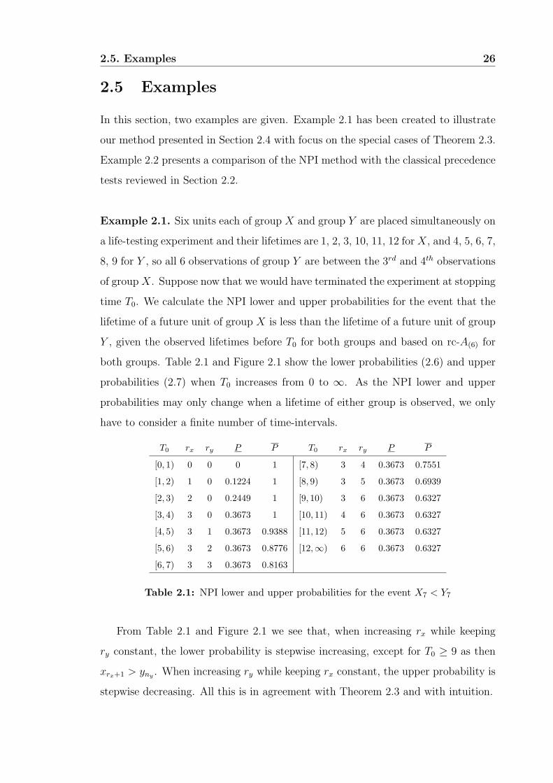
Example 2.1. Six units each of group X and group Y are placed simultaneously on
a life-testing experiment and their lifetimes are 1, 2, 3, 10, 11, 12 forX, and 4, 5, 6, 7,
8, 9 for Y , so all 6 observations of group Y are between the 3rd and 4th observations
of groupX. Suppose now that we would have terminated the experiment at stopping
time T0. We calculate the NPI lower and upper probabilities for the event that the
lifetime of a future unit of group X is less than the lifetime of a future unit of group
Y , given the observed lifetimes before T0 for both groups and based on rc-A(6) for
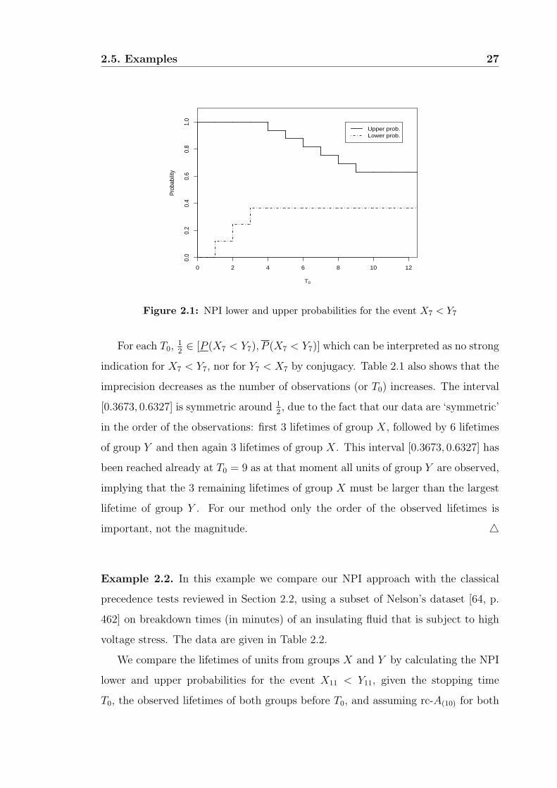
both groups. Table 2.1 and Figure 2.1 show the lower probabilities (2.6) and upper
probabilities (2.7) when T0 increases from 0 to ∞. As the NPI lower and upper
probabilities may only change when a lifetime of either group is observed, we only
have to consider a finite number of time-intervals.
T0 rx ry P P T0 rx ry P P
[0, 1) 0 0 0 1 [7, 8) 3 4 0.3673 0.7551
[1, 2) 1 0 0.1224 1 [8, 9) 3 5 0.3673 0.6939
[2, 3) 2 0 0.2449 1 [9, 10) 3 6 0.3673 0.6327
[3, 4) 3 0 0.3673 1 [10, 11) 4 6 0.3673 0.6327
[4, 5) 3 1 0.3673 0.9388 [11, 12) 5 6 0.3673 0.6327
[5, 6) 3 2 0.3673 0.8776 [12,∞) 6 6 0.3673 0.6327
[6, 7) 3 3 0.3673 0.8163
Table 2.1: NPI lower and upper probabilities for the event X7 < Y7
From Table 2.1 and Figure 2.1 we see that, when increasing rx while keeping
ry constant, the lower probability is stepwise increasing, except for T0 ≥ 9 as then
xrx+1 > yny. When increasing ry while keeping rx constant, the upper probability is
stepwise decreasing. All this is in agreement with Theorem 2.3 and with intuition.
2.5. Examples 27
0 2 4 6 8 10 12
0.0
0.2
0.4
0.6
0.8
1.0
T0
Pro
babi
lity
Upper prob.Lower prob.
Figure 2.1: NPI lower and upper probabilities for the event X7 < Y7
For each T0,12∈ [P (X7 < Y7), P (X7 < Y7)] which can be interpreted as no strong
indication for X7 < Y7, nor for Y7 < X7 by conjugacy. Table 2.1 also shows that the
imprecision decreases as the number of observations (or T0) increases. The interval
[0.3673, 0.6327] is symmetric around 12, due to the fact that our data are ‘symmetric’
in the order of the observations: first 3 lifetimes of group X, followed by 6 lifetimes
of group Y and then again 3 lifetimes of group X. This interval [0.3673, 0.6327] has
been reached already at T0 = 9 as at that moment all units of group Y are observed,
implying that the 3 remaining lifetimes of group X must be larger than the largest
lifetime of group Y . For our method only the order of the observed lifetimes is
important, not the magnitude. 4
Example 2.2. In this example we compare our NPI approach with the classical
precedence tests reviewed in Section 2.2, using a subset of Nelson’s dataset [64, p.
462] on breakdown times (in minutes) of an insulating fluid that is subject to high
voltage stress. The data are given in Table 2.2.
We compare the lifetimes of units from groups X and Y by calculating the NPI
lower and upper probabilities for the event X11 < Y11, given the stopping time
T0, the observed lifetimes of both groups before T0, and assuming rc-A(10) for both
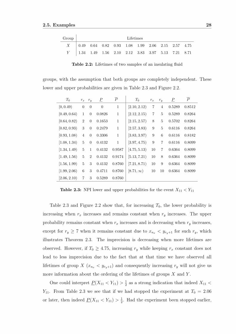
2.5. Examples 28
Group Lifetimes
X 0.49 0.64 0.82 0.93 1.08 1.99 2.06 2.15 2.57 4.75
Y 1.34 1.49 1.56 2.10 2.12 3.83 3.97 5.13 7.21 8.71
Table 2.2: Lifetimes of two samples of an insulating fluid
groups, with the assumption that both groups are completely independent. These
lower and upper probabilities are given in Table 2.3 and Figure 2.2.
T0 rx ry P P T0 rx ry P P
[0, 0.49) 0 0 0 1 [2.10, 2.12) 7 4 0.5289 0.8512
[0.49, 0.64) 1 0 0.0826 1 [2.12, 2.15) 7 5 0.5289 0.8264
[0.64, 0.82) 2 0 0.1653 1 [2.15, 2.57) 8 5 0.5702 0.8264
[0.82, 0.93) 3 0 0.2479 1 [2.57, 3.83) 9 5 0.6116 0.8264
[0.93, 1.08) 4 0 0.3306 1 [3.83, 3.97) 9 6 0.6116 0.8182
[1.08, 1.34) 5 0 0.4132 1 [3.97, 4.75) 9 7 0.6116 0.8099
[1.34, 1.49) 5 1 0.4132 0.9587 [4.75, 5.13) 10 7 0.6364 0.8099
[1.49, 1.56) 5 2 0.4132 0.9174 [5.13, 7.21) 10 8 0.6364 0.8099
[1.56, 1.99) 5 3 0.4132 0.8760 [7.21, 8.71) 10 9 0.6364 0.8099
[1.99, 2.06) 6 3 0.4711 0.8760 [8.71,∞) 10 10 0.6364 0.8099
[2.06, 2.10) 7 3 0.5289 0.8760
Table 2.3: NPI lower and upper probabilities for the event X11 < Y11
Table 2.3 and Figure 2.2 show that, for increasing T0, the lower probability is
increasing when rx increases and remains constant when ry increases. The upper
probability remains constant when rx increases and is decreasing when ry increases,
except for ry ≥ 7 when it remains constant due to xnx< yry+1 for such ry, which
illustrates Theorem 2.3. The imprecision is decreasing when more lifetimes are
observed. However, if T0 ≥ 4.75, increasing ry while keeping rx constant does not
lead to less imprecision due to the fact that at that time we have observed all
lifetimes of group X (xnx< yry+1) and consequently increasing ry will not give us
more information about the ordering of the lifetimes of groups X and Y .
One could interpret P (X11 < Y11) >12as a strong indication that indeed X11 <
Y11. From Table 2.3 we see that if we had stopped the experiment at T0 = 2.06
or later, then indeed P (X11 < Y11) >12. Had the experiment been stopped earlier,
2.5. Examples 29
0 2 4 6 8
0.0
0.2
0.4
0.6
0.8
1.0
T0
Pro
babi
lity
Upper prob.Lower prob.
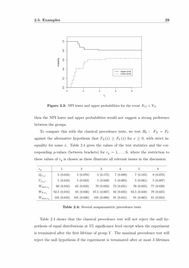
Figure 2.2: NPI lower and upper probabilities for the event X11 < Y11
then the NPI lower and upper probabilities would not suggest a strong preference
between the groups.
To compare this with the classical precedence tests, we test H0 : FX = FY
against the alternative hypothesis that FX(x) ≥ FY (x) for x ≥ 0, with strict in-
equality for some x. Table 2.4 gives the values of the test statistics and the cor-
responding p-values (between brackets) for ry = 1, . . . , 6, where the restriction to
these values of ry is chosen as these illustrate all relevant issues in the discussion.
ry 1 2 3 4 5 6
Q(ry) 5 (0.016) 5 (0.070) 5 (0.175) 7 (0.089) 7 (0.185) 9 (0.070)
U(ry) 5 (0.016) 5 (0.033) 5 (0.049) 5 (0.065) 5 (0.081) 5 (0.097)
Wmin,ry 60 (0.016) 65 (0.022) 70 (0.033) 73 (0.031) 76 (0.035) 77 (0.029)
WE,ry 82.5 (0.016) 85 (0.036) 87.5 (0.067) 82 (0.035) 83.5 (0.048) 79 (0.025)
Wmax,ry 105 (0.016) 105 (0.036) 105 (0.086) 91 (0.041) 91 (0.065) 81 (0.024)
Table 2.4: Several nonparametric precedence tests
Table 2.4 shows that the classical precedence test will not reject the null hy-
pothesis of equal distributions at 5% significance level except when the experiment
is terminated after the first lifetime of group Y . The maximal precedence test will
reject the null hypothesis if the experiment is terminated after at most 3 lifetimes
2.6. Concluding remarks 30
of group Y . Intuitively, this is logical as we have first observed 5 lifetimes of group
X before the first observation of group Y and no observed lifetimes of group X
between the first and third observation of group Y . In this example, Wilcoxon’s
minimal rank-sum precedence test always rejects the null hypothesis at 5% signifi-
cance level. However, Wilcoxon’s maximal and expected rank-sum precedence tests
reject the null hypothesis only for some values of ry. We saw before that according
to our NPI approach there is an indication that X11 < Y11 when the experiment is
terminated after T0 = 2.06. The results of the classical, Wilcoxon’s maximal and
expected rank-sum precedence tests at this T0 are not in agreement with this but
the maximal and Wilcoxon’s minimal rank-sum precedence tests are. As the NPI
approach is fundamentally different to these hypothesis tests, studying the results
of both might provide useful insights for practical problems. 4
2.6 Concluding remarks
The lower and upper probabilities for predictive precedence testing for two groups,
presented in this chapter, fit in the NPI framework and as such they have strong con-
sistency properties in theory of interval probability [1]. This approach provides an
attractive alternative to the more established methods for nonparametric precedence
testing [5], as instead of testing a null hypothesis the inference directly considers a
comparison of the next observations from the groups considered.
When considering the NPI lower and upper probabilities for the event Xnx+1 <
Yny+1 as a function of the stopping time T0, we showed that these probabilities can
only change at observed lifetimes for groups X or Y . In particular, we showed that,
except for one special case, the lower probability is strictly increasing in rx while
keeping ry constant, and the upper probability is strictly decreasing in ry while
keeping rx constant. As a consequence of this, the imprecision is decreasing as a
function of the number of observed lifetimes and hence as a function of time.
An important issue in statistics is guidance on required design of experiments,
in this situation the numbers of units to be used for both groups and choice of
the stopping time for the experiment. Due to the rather minimal assumptions
2.6. Concluding remarks 31
underlying our NPI approach, with the inferences largely based on observed data,
it does not offer a satisfactory solution to this important question. However, once
an experiment is underway, one can monitor the lower and upper probabilities as
presented in this chapter, and one can stop the experiment if one judges these to
indicate a strong enough preference between the two groups. Of course, before any
data become available, one can study some design issues, e.g. the minimum required
number of observations to possibly get a lower probability greater than a half, but
as these would be based on most or least favourable configurations of the not yet
observed data, indications from such studies might be of little practical value.
Chapter 3
Multiple comparisons with early
termination
3.1 Introduction
In Chapter 2 we introduced NPI for comparison of two groups with early termination
of experiments. In this chapter, we consider the situation where units from several
groups (k ≥ 2) are simultaneously placed on a life-testing experiment, and decisions
may be needed before all units have failed due to cost or time considerations.
Balakrishnan and Ng [5] described several nonparametric precedence tests based
on the hypothesis of equal lifetime distributions. In Section 3.2 we briefly describe
some of these classical methods. In Sections 3.3, 3.4 and 3.5 we present NPI for
precedence testing for k ≥ 2 groups in order to select the best group, the subset
of best groups and the subset including the best group, respectively. Examples are
provided throughout to illustrate our method and to compare it with the classical
methods. Section 3.6 contains some concluding remarks.
3.2 Classical methods
When the null hypothesis of the equality (homogeneity) of two (or more) popu-
lations (e.g. processes, treatments) is rejected, one may want to identify which of
these populations is the best. Balakrishnan and Ng [5] introduced several nonpara-
32
3.2. Classical methods 33
metric tests for this selection problem when an early decision is required (called
precedence testing). Below we briefly describe these precedence selection methods
using notation and definitions from Balakrishnan and Ng [5].
Suppose that we have independent random samples from k ≥ 2 different pop-
ulations. Let Xj,ij (ij = 1, . . . , nj) be the lifetime of the ijth component of a ran-
dom sample from population πj with distribution function Fj (j = 1, . . . , k). We
have N =∑k
j=1 nj units placed simultaneously on a lifetime testing experiment.
The question of interest is to test whether these populations are homogeneous, i.e.
H0 : F1 = F2 = . . . = Fk against the alternative that population πi is the best
(longer life), that is HAi : Fi < Fj for all j 6= i and j = 1, . . . , k. That is, it can be
concluded that Xi, a random quantity representing the lifetime of a unit of popula-
tion i, is stochastically larger than Xj (i.e. Xi st Xj) if and only if Fi(x) ≤ Fj(x)
for all x ≥ 0 with strict inequality for at least one x, consequently Fi < Fj.
In precedence testing the aim is to reach a decision before all units have failed.
So the experiment is terminated as soon as the rith failure from group i is observed,
where ri = bniqc for i = 1, . . . , k and 0 < q < 1, where bac is the largest integer
not greater than a. Consequently, the stopping time T0 can be defined as T0 =
min1≤i≤k
Xi,(ri), where Xi,(ri) is the rith order statistic of sample i.
Suppose now that the experiment is terminated at sample i, i.e. T0 = Xi,(ri),
then the ordinary precedence statistic [6] is defined as
Q∗(i) = min1≤j≤kj 6=i
(
Q(i)j /nj
)
(3.1)
where Q(i)j is the number of failures observed before Xi,(r) from the sample j (j =
1, . . . , k, j 6= i). Small values of Q∗(i) will lead to rejection of the null hypothesis
H0. In this case one can choose HAj (πj is the best) if and only if (Q(i)j /nj) = Q∗(i)
for j 6= i and T0 = Xi,(ri). If for two or more samples the statistic (Q(i)j /nj) is equal
to Q∗(i) then one of the corresponding populations is randomly selected as the best.
Now letD(i)j,s be the number of failures of sample j that occur between the (s−1)th
and sth failure of group i, s = 2, . . . , ri and let D(i)j,1 be the number of failures of
sample j that occur before the first failure of group i. Let W(i)j (j = 1, . . . , k, j 6= i)

3.2. Classical methods 34
be a random quantity defined by
W(i)j =
1
2nj(nj + 2ri + 1)− (ri + 1)
ri∑
s=1
D(i)j,s +
ri∑
s=1
s D(i)j,s
Then the minimal Wilcoxon rank-sum statistic [68] is given by
W ∗(i) = max1≤j≤k
j 6=i
W(i)j − E[W
(i)j |H0]
√
V ar[W(i)j |H0]
(3.2)
where E[W(i)j |H0] and V ar[W
(i)j |H0] are the expected value and the variance of the
statistic W(i)j under H0. Large values of W ∗(i) will lead to rejection of the null
hypothesis, in which case one can choose the alternative hypothesis HAj (πj is the
best) if and only if T0 = Xi,(ri) and (W(i)j −E[W
(i)j |H0])(V ar[W
(i)j |H0])
−1/2 = W ∗(i),
for j 6= i.
In this chapter we will focus on the balanced-sample case only (nj = n for all
j) when we compare our method with the classical precedence selection procedures,
since these classical procedures may not be effective when the sample sizes vary
much [5, pp. 226, 265]. For the balanced-sample case, the statistics in (3.1) and
(3.2) reduce to Q∗(i) = minQ(i)j and W ∗(i) = maxW
(i)j , over all j = 1, . . . , k and
j 6= i, respectively. For more details we refer to Balakrishnan and Ng [5]. It
should be emphasized that the NPI method presented in this chapter is equally
straightforward to implement for balanced-sample and unbalanced-sample cases.
A somewhat separate, yet strongly related, branch of statistical research is so-
called ‘selection methods’, which also have the explicit target to select a single
‘best’ group or population or a subset of groups, along the same lines considered
in this chapter. The two main classical approaches in this field are indifference
zone selection [11, 12] and subset selection [38], which were combined by Verheijen
et al. [75]. Coolen and van der Laan [25] presented NPI methods for selection,
in this chapter we follow the same approach with the generalization to allow early
termination of the experiments, hence linking to the classical concepts of precedence
testing.
3.3. Selecting the best group 35
3.3 Selecting the best group
In precedence testing, units of all groups are placed simultaneously on a life-testing
experiment, and failures are observed as they arise during the experiment. The
experiment is terminated as soon as a certain stop criterion has been reached, so
the lifetimes of some units are typically right-censored. We assume that this stop
criterion is expressed in terms of a stopping time T0, but if instead a number of
failures were used as stop criterion then this would not affect our method, as it
is of no relevance in NPI how T0 is determined as long as T0 contains no further
information on the residual event times beyond T0 for right-censored units. In
Chapter 2 we introduced NPI for precedence testing for two groups. In this chapter
we extend NPI to precedence testing for k ≥ 2 groups in order to select the best
group, the subset of best groups, and the subset including the best group. Again we
use the assumption rc-A(n) required for precedence testing which is given in Theorem
2.1.
Suppose we have k ≥ 2 groups and nj + 1 random quantities from group j,
denoted by Xj,ij where ij = 1, 2, . . . , nj , nj + 1, j = 1, 2, . . . , k. For each group j,
nj units are put on a lifetime experiment and we are interested in the behaviour of
the future random variable Xj,nj+1. Therefore, we have N =∑k
j=1 nj units on the
lifetime experiment and one may want to terminate the experiment at certain time
T0. Let 0 = xj,0 < xj,1 < xj,2 < . . . < xj,rj ≤ T0 < ∞ be the ordered observed values
(failures) from group j, j = 1, . . . , k.
These observed values from group j produce rj + 2 intervals, where the first rj
intervals are defined by Ijij = (xj,ij−1, xj,ij), ij = 1, . . . , rj , j = 1, . . . , k, and the
remaining intervals are defined by Ijrj+1 = (xj,rj ,∞), Ijrj+2 = (T0,∞), notice that
these are overlapping. Let L(Ijij) and U(Ijij) be the lower and the upper bounds
for the interval Ijij , ij = 1, . . . , rj + 2, j = 1, . . . , k. That is, L(Ijij) = xj,ij−1 for
ij = 1, . . . , rj + 1 and L(Ijrj+2) = T0. Similar for the upper bound, U(Ijij) = xj,ij
for ij = 1, . . . , rj , and U(Ijrj+1) = U(Ijrj+2) = ∞. Here the intervals Ijij are open
intervals, but in future when we mention the (left or right) end points we actually
mean the limit end points which are not included in these open intervals.
For our NPI approach we assume rc-A(nj) for each group [27]. Beyond the data,
3.3. Selecting the best group 36
our method requires the exchangeability assumptions of the random variables per
group to be met. We also assume that groups are completely independent. We
will specify partially the probability distribution for a future quantity, Xj,nj+1, j =
1, . . . , k, using M -functions presented in Theorem 2.1.
Theorem 3.1 gives the NPI lower and upper probability for the event that the
lifetime of the next observation from one group, say l, is greater than the lifetime
of the next observation from each other group, that is
P (l) = P
(
Xl,nl+1 = max1≤j≤k
Xj,nj+1
)
and P(l)
= P
(
Xl,nl+1 = max1≤j≤k
Xj,nj+1
)
Theorem 3.1. The NPI lower and upper probabilities for the event that the life-
time of the next observation from group l is greater than the lifetime of the next
observation from each other group are
P (l) =1
k∏
j=1
(nj + 1)
rl∑
il=1
k∏
j=1
j 6=l
rj∑
ij=1
1xj,ij < xl,il+ (nl − rl)k∏
j=1
j 6=l
rj
(3.3)
P(l)
=1
k∏
j=1
(nj + 1)
rl∑
il=1
k∏
j=1
j 6=l
1 +
rj∑
ij=1
1xj,ij < xl,il
+nl − rl + 1
nl + 1(3.4)
Proof. The proof is a special case of the proof of Theorem 3.3, with S (in Theorem
3.3) now only containing group l.
3.3.1 Special cases
In this part, we discuss some special cases of these lower and upper probabilities,
which are easily verified from (3.3) and (3.4).
1. If rl ≥ 0 and there exists at least one j 6= l for which rj = 0, then the NPI
lower probability is P (l) = 0, since we have not seen any failure from group
j 6= l. Hence, we cannot exclude the possibility that we would never see a
failure from group(s) j 6= l. Further, if rl = 0 then the upper probability P(l)
is equal to one.
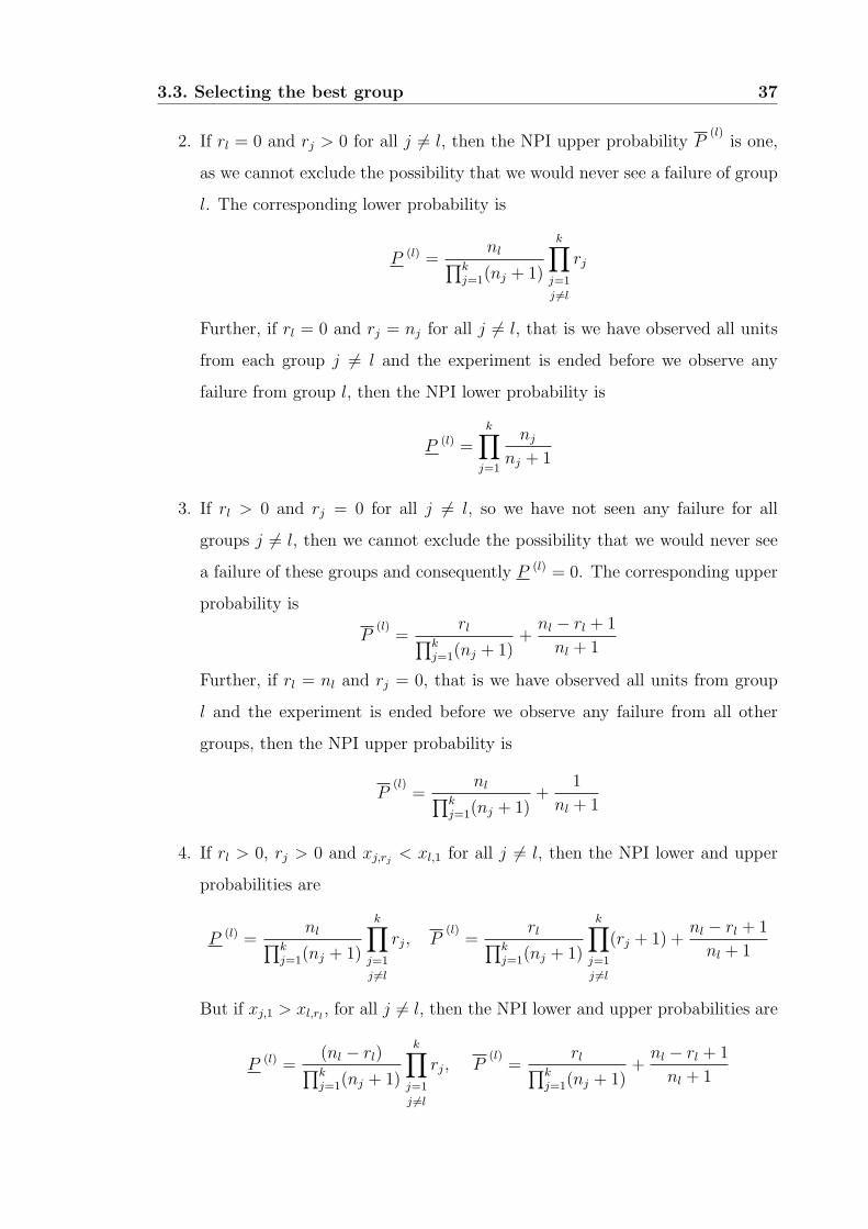
3.3. Selecting the best group 37
2. If rl = 0 and rj > 0 for all j 6= l, then the NPI upper probability P(l)
is one,
as we cannot exclude the possibility that we would never see a failure of group
l. The corresponding lower probability is
P (l) =nl
∏kj=1(nj + 1)
k∏
j=1
j 6=l
rj
Further, if rl = 0 and rj = nj for all j 6= l, that is we have observed all units
from each group j 6= l and the experiment is ended before we observe any
failure from group l, then the NPI lower probability is
P (l) =k∏
j=1
nj
nj + 1
3. If rl > 0 and rj = 0 for all j 6= l, so we have not seen any failure for all
groups j 6= l, then we cannot exclude the possibility that we would never see
a failure of these groups and consequently P (l) = 0. The corresponding upper
probability is
P(l)
=rl
∏kj=1(nj + 1)
+nl − rl + 1
nl + 1
Further, if rl = nl and rj = 0, that is we have observed all units from group
l and the experiment is ended before we observe any failure from all other
groups, then the NPI upper probability is
P(l)
=nl
∏kj=1(nj + 1)
+1
nl + 1
4. If rl > 0, rj > 0 and xj,rj < xl,1 for all j 6= l, then the NPI lower and upper
probabilities are
P (l) =nl
∏kj=1(nj + 1)
k∏
j=1
j 6=l
rj, P(l)
=rl
∏kj=1(nj + 1)
k∏
j=1
j 6=l
(rj + 1) +nl − rl + 1
nl + 1
But if xj,1 > xl,rl , for all j 6= l, then the NPI lower and upper probabilities are
P (l) =(nl − rl)
∏kj=1(nj + 1)
k∏
j=1
j 6=l
rj, P(l)
=rl
∏kj=1(nj + 1)
+nl − rl + 1
nl + 1
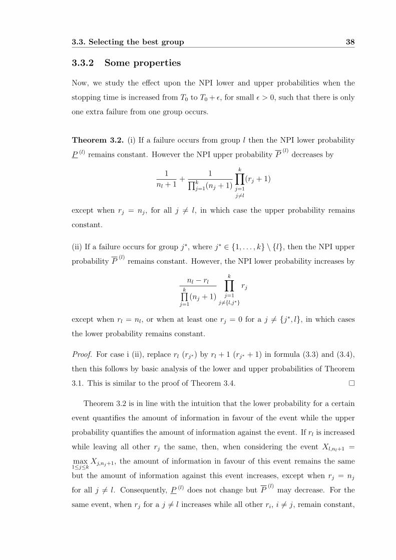
3.3. Selecting the best group 38
3.3.2 Some properties
Now, we study the effect upon the NPI lower and upper probabilities when the
stopping time is increased from T0 to T0 + ε, for small ε > 0, such that there is only
one extra failure from one group occurs.
Theorem 3.2. (i) If a failure occurs from group l then the NPI lower probability
P (l) remains constant. However the NPI upper probability P(l)
decreases by
1
nl + 1+
1∏k
j=1(nj + 1)
k∏
j=1
j 6=l
(rj + 1)
except when rj = nj, for all j 6= l, in which case the upper probability remains
constant.
(ii) If a failure occurs for group j∗, where j∗ ∈ 1, . . . , k \ l, then the NPI upper
probability P(l)
remains constant. However, the NPI lower probability increases by
nl − rlk∏
j=1
(nj + 1)
k∏
j=1
j 6=l,j∗
rj
except when rl = nl, or when at least one rj = 0 for a j 6= j∗, l, in which cases
the lower probability remains constant.
Proof. For case i (ii), replace rl (rj∗) by rl + 1 (rj∗ + 1) in formula (3.3) and (3.4),
then this follows by basic analysis of the lower and upper probabilities of Theorem
3.1. This is similar to the proof of Theorem 3.4.
Theorem 3.2 is in line with the intuition that the lower probability for a certain
event quantifies the amount of information in favour of the event while the upper
probability quantifies the amount of information against the event. If rl is increased
while leaving all other rj the same, then, when considering the event Xl,nl+1 =
max1≤j≤k
Xj,nj+1, the amount of information in favour of this event remains the same
but the amount of information against this event increases, except when rj = nj
for all j 6= l. Consequently, P (l) does not change but P(l)
may decrease. For the
same event, when rj for a j 6= l increases while all other ri, i 6= j, remain constant,
3.3. Selecting the best group 39
the amount of information in favour of the event increases, except when rl = nl or
when there exists a j 6= l, j∗ for which rj = 0, while the amount of information
against the event remains the same. Consequently, P (l) may increase but P(l)
does
not change.
At any value of T0, we can state that the data provide a strong indication that
group l is the best if P (l) > P(j)
for all j 6= l. Of course, this may not occur,
and we may be happy to have data providing a weak indication that group l is
the best. It might seem attractive to state that, if P (l) > P (j) and P(l)
> P(j)
for
all j 6= l, there would be a weak indication that group l is the best. Indeed, if
one has to select one group and there is a group for which such a weak indication
of being best holds, then that is the natural candidate. However, such a weak
indication can be very weak indeed, in particular as it can already occur for relatively
small T0, with P (l) positive but very small. If such a weak indication holds for
one group, and in addition one judges the lower probability of this group being
best to be sufficiently high, then it seems a reasonable basis for the choice of this
group as being the best. In all these considerations, it is an advantage that the the
difference between corresponding lower and upper probabilities (P(l) −P (l)) reflects
the amount of information available, and it decreases if more relevant information
becomes available. If one judges this difference to be too large, or if one judges each
lower probability of a group being best too small to base a choice on the information
available, then clearly one must either get more information, e.g. by continuing the
experiment or try to repeat the experiment with more units, or one could explore
the use of other statistical approaches with more modeling assumptions.
In discussions in the examples in this chapter, we will call one group ‘better’
than another, or ‘best’, if the first of these conditions is satisfied, of course the use
of ‘better’ and ‘best’ must be interpreted with care as these judgments are just based
on direct comparison of one next observation for each group according to the NPI
method.
Below two examples are given to illustrate our method for selecting the best
group and to compare it with the classical methods reviewed in Section 3.2.
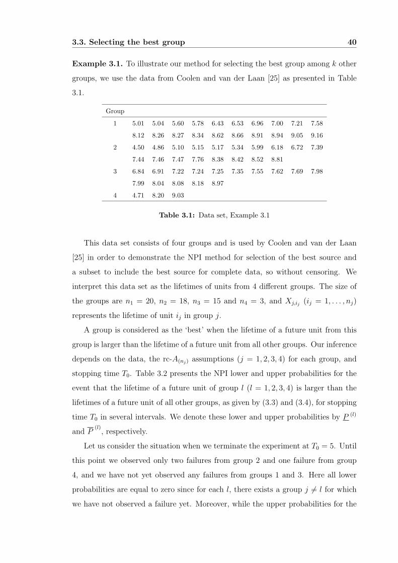
3.3. Selecting the best group 40
Example 3.1. To illustrate our method for selecting the best group among k other
groups, we use the data from Coolen and van der Laan [25] as presented in Table
3.1.
Group
1 5.01 5.04 5.60 5.78 6.43 6.53 6.96 7.00 7.21 7.58
8.12 8.26 8.27 8.34 8.62 8.66 8.91 8.94 9.05 9.16
2 4.50 4.86 5.10 5.15 5.17 5.34 5.99 6.18 6.72 7.39
7.44 7.46 7.47 7.76 8.38 8.42 8.52 8.81
3 6.84 6.91 7.22 7.24 7.25 7.35 7.55 7.62 7.69 7.98
7.99 8.04 8.08 8.18 8.97
4 4.71 8.20 9.03
Table 3.1: Data set, Example 3.1
This data set consists of four groups and is used by Coolen and van der Laan
[25] in order to demonstrate the NPI method for selection of the best source and
a subset to include the best source for complete data, so without censoring. We
interpret this data set as the lifetimes of units from 4 different groups. The size of
the groups are n1 = 20, n2 = 18, n3 = 15 and n4 = 3, and Xj,ij (ij = 1, . . . , nj)
represents the lifetime of unit ij in group j.
A group is considered as the ‘best’ when the lifetime of a future unit from this
group is larger than the lifetime of a future unit from all other groups. Our inference
depends on the data, the rc-A(nj) assumptions (j = 1, 2, 3, 4) for each group, and
stopping time T0. Table 3.2 presents the NPI lower and upper probabilities for the
event that the lifetime of a future unit of group l (l = 1, 2, 3, 4) is larger than the
lifetimes of a future unit of all other groups, as given by (3.3) and (3.4), for stopping
time T0 in several intervals. We denote these lower and upper probabilities by P (l)
and P(l), respectively.
Let us consider the situation when we terminate the experiment at T0 = 5. Until
this point we observed only two failures from group 2 and one failure from group
4, and we have not yet observed any failures from groups 1 and 3. Here all lower
probabilities are equal to zero since for each l, there exists a group j 6= l for which
we have not observed a failure yet. Moreover, while the upper probabilities for the
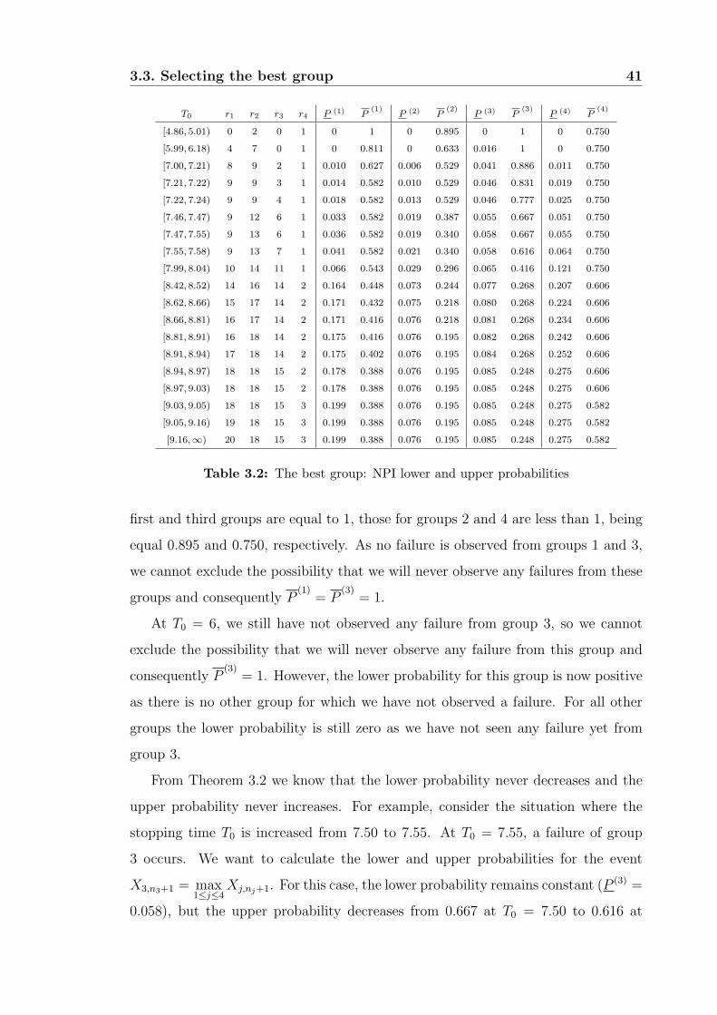
3.3. Selecting the best group 41
T0 r1 r2 r3 r4 P (1) P(1)
P (2) P(2)
P (3) P(3)
P (4) P(4)
[4.86, 5.01) 0 2 0 1 0 1 0 0.895 0 1 0 0.750
[5.99, 6.18) 4 7 0 1 0 0.811 0 0.633 0.016 1 0 0.750
[7.00, 7.21) 8 9 2 1 0.010 0.627 0.006 0.529 0.041 0.886 0.011 0.750
[7.21, 7.22) 9 9 3 1 0.014 0.582 0.010 0.529 0.046 0.831 0.019 0.750
[7.22, 7.24) 9 9 4 1 0.018 0.582 0.013 0.529 0.046 0.777 0.025 0.750
[7.46, 7.47) 9 12 6 1 0.033 0.582 0.019 0.387 0.055 0.667 0.051 0.750
[7.47, 7.55) 9 13 6 1 0.036 0.582 0.019 0.340 0.058 0.667 0.055 0.750
[7.55, 7.58) 9 13 7 1 0.041 0.582 0.021 0.340 0.058 0.616 0.064 0.750
[7.99, 8.04) 10 14 11 1 0.066 0.543 0.029 0.296 0.065 0.416 0.121 0.750
[8.42, 8.52) 14 16 14 2 0.164 0.448 0.073 0.244 0.077 0.268 0.207 0.606
[8.62, 8.66) 15 17 14 2 0.171 0.432 0.075 0.218 0.080 0.268 0.224 0.606
[8.66, 8.81) 16 17 14 2 0.171 0.416 0.076 0.218 0.081 0.268 0.234 0.606
[8.81, 8.91) 16 18 14 2 0.175 0.416 0.076 0.195 0.082 0.268 0.242 0.606
[8.91, 8.94) 17 18 14 2 0.175 0.402 0.076 0.195 0.084 0.268 0.252 0.606
[8.94, 8.97) 18 18 15 2 0.178 0.388 0.076 0.195 0.085 0.248 0.275 0.606
[8.97, 9.03) 18 18 15 2 0.178 0.388 0.076 0.195 0.085 0.248 0.275 0.606
[9.03, 9.05) 18 18 15 3 0.199 0.388 0.076 0.195 0.085 0.248 0.275 0.582
[9.05, 9.16) 19 18 15 3 0.199 0.388 0.076 0.195 0.085 0.248 0.275 0.582
[9.16,∞) 20 18 15 3 0.199 0.388 0.076 0.195 0.085 0.248 0.275 0.582
Table 3.2: The best group: NPI lower and upper probabilities
first and third groups are equal to 1, those for groups 2 and 4 are less than 1, being
equal 0.895 and 0.750, respectively. As no failure is observed from groups 1 and 3,
we cannot exclude the possibility that we will never observe any failures from these
groups and consequently P(1)
= P(3)
= 1.
At T0 = 6, we still have not observed any failure from group 3, so we cannot
exclude the possibility that we will never observe any failure from this group and
consequently P(3)
= 1. However, the lower probability for this group is now positive
as there is no other group for which we have not observed a failure. For all other
groups the lower probability is still zero as we have not seen any failure yet from
group 3.
From Theorem 3.2 we know that the lower probability never decreases and the
upper probability never increases. For example, consider the situation where the
stopping time T0 is increased from 7.50 to 7.55. At T0 = 7.55, a failure of group
3 occurs. We want to calculate the lower and upper probabilities for the event
X3,n3+1 = max1≤j≤4
Xj,nj+1. For this case, the lower probability remains constant (P (3) =
0.058), but the upper probability decreases from 0.667 at T0 = 7.50 to 0.616 at
3.3. Selecting the best group 42
T0 = 7.55, which illustrates Theorem 3.2(i). However, for the event X1,n1+1 =
max1≤j≤4
Xj,nj+1 the upper probability remains constant (P(1)
= 0.582) but the lower
probability increases from 0.036 at T0 = 7.50 to 0.041 at T0 = 7.55, which illustrates
Theorem 3.2(ii).
There are some special cases when all lower and upper probabilities remain con-
stant when a failure occurs from any group. For example, at T0 = 9.03 we have
observed all units from all groups except the first group which still has two units
which have not failed. Let l = 1 and assume we will allow for an extra failure to
occur. Here of course the failure must be from the first group (T0 = 9.05). In this
case all lower and upper probabilities remain as they were at T0 = 9.03, as the
amount of information in favour and against the event does not change. In fact, all
lower and upper probabilities do not change anymore after 9.03.
At T0 = 8.81, we have observed failure times of all units from the second group.
Now consider l = 2 and let the stopping time increase to 8.91, so that we observe
an extra failure of group 1. In this case the lower and upper probabilities remain
constant (P (2) = 0.076 and P(2)
= 0.195). In fact, any failure from other groups
after we have observed failures of all units from group 2 will not affect the lower and
upper probabilities P (2) and P(2).
From T0 = 7.55 on, the fourth group has the greatest lower and upper probabil-
ities. However, from the beginning of the experiment till T0 = 7.22 the third group
has the greatest lower and upper probabilities. Which means that at T0 ≤ 7.22,
there is a weak indication that group 3 is best, since P (j) < P (3) < P(j)
< P(3)
for
j = 1, 2, 4, however, there is a weak indication that group 4 is best for T0 ≥ 7.55,
since P (j) < P (4) < P(j)
< P(4)
for j = 1, 2, 3. Also we can note that P(3)
remains
equal to 1 for quite a long time, since the first failure from the third group occurs
relatively late.
The imprecision decreases as the stopping time T0 increases, which reflects the
amount of information we have (Table 3.2). For example, we can see that the fourth
group has larger imprecision as there are only a few observations in this group.
A crucial question is how to make decisions using these NPI lower and upper
probabilities. If we observe all units from groups 2, 3 and 4, so for T0 ≥ 9.03, we see
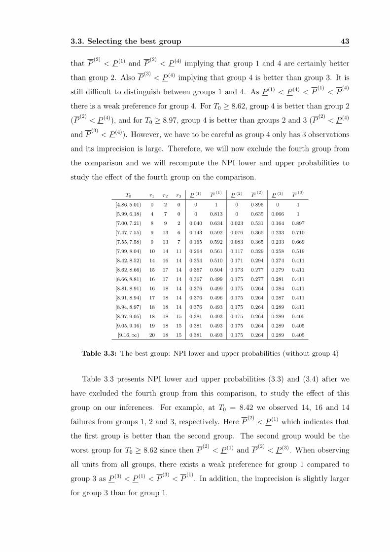
3.3. Selecting the best group 43
that P(2)
< P (1) and P(2)
< P (4) implying that group 1 and 4 are certainly better
than group 2. Also P(3)
< P (4) implying that group 4 is better than group 3. It is
still difficult to distinguish between groups 1 and 4. As P (1) < P (4) < P(1)
< P(4)
there is a weak preference for group 4. For T0 ≥ 8.62, group 4 is better than group 2
(P(2)
< P (4)), and for T0 ≥ 8.97, group 4 is better than groups 2 and 3 (P(2)
< P (4)
and P(3)
< P (4)). However, we have to be careful as group 4 only has 3 observations
and its imprecision is large. Therefore, we will now exclude the fourth group from
the comparison and we will recompute the NPI lower and upper probabilities to
study the effect of the fourth group on the comparison.
T0 r1 r2 r3 P (1) P(1)
P (2) P(2)
P (3) P(3)
[4.86, 5.01) 0 2 0 0 1 0 0.895 0 1
[5.99, 6.18) 4 7 0 0 0.813 0 0.635 0.066 1
[7.00, 7.21) 8 9 2 0.040 0.634 0.023 0.531 0.164 0.897
[7.47, 7.55) 9 13 6 0.143 0.592 0.076 0.365 0.233 0.710
[7.55, 7.58) 9 13 7 0.165 0.592 0.083 0.365 0.233 0.669
[7.99, 8.04) 10 14 11 0.264 0.561 0.117 0.329 0.258 0.519
[8.42, 8.52) 14 16 14 0.354 0.510 0.171 0.294 0.274 0.411
[8.62, 8.66) 15 17 14 0.367 0.504 0.173 0.277 0.279 0.411
[8.66, 8.81) 16 17 14 0.367 0.499 0.175 0.277 0.281 0.411
[8.81, 8.91) 16 18 14 0.376 0.499 0.175 0.264 0.284 0.411
[8.91, 8.94) 17 18 14 0.376 0.496 0.175 0.264 0.287 0.411
[8.94, 8.97) 18 18 14 0.376 0.493 0.175 0.264 0.289 0.411
[8.97, 9.05) 18 18 15 0.381 0.493 0.175 0.264 0.289 0.405
[9.05, 9.16) 19 18 15 0.381 0.493 0.175 0.264 0.289 0.405
[9.16,∞) 20 18 15 0.381 0.493 0.175 0.264 0.289 0.405
Table 3.3: The best group: NPI lower and upper probabilities (without group 4)
Table 3.3 presents NPI lower and upper probabilities (3.3) and (3.4) after we
have excluded the fourth group from this comparison, to study the effect of this
group on our inferences. For example, at T0 = 8.42 we observed 14, 16 and 14
failures from groups 1, 2 and 3, respectively. Here P(2)
< P (1) which indicates that
the first group is better than the second group. The second group would be the
worst group for T0 ≥ 8.62 since then P(2)
< P (1) and P(2)
< P (3). When observing
all units from all groups, there exists a weak preference for group 1 compared to
group 3 as P (3) < P (1) < P(3)
< P(1). In addition, the imprecision is slightly larger
for group 3 than for group 1.
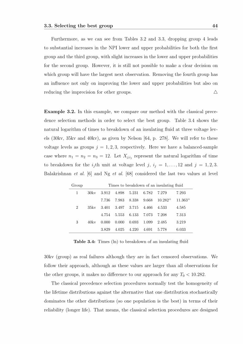
3.3. Selecting the best group 44
Furthermore, as we can see from Tables 3.2 and 3.3, dropping group 4 leads
to substantial increases in the NPI lower and upper probabilities for both the first
group and the third group, with slight increases in the lower and upper probabilities
for the second group. However, it is still not possible to make a clear decision on
which group will have the largest next observation. Removing the fourth group has
an influence not only on improving the lower and upper probabilities but also on
reducing the imprecision for other groups. 4
Example 3.2. In this example, we compare our method with the classical prece-
dence selection methods in order to select the best group. Table 3.4 shows the
natural logarithm of times to breakdown of an insulating fluid at three voltage lev-
els (30kv, 35kv and 40kv), as given by Nelson [64, p. 278]. We will refer to these
voltage levels as groups j = 1, 2, 3, respectively. Here we have a balanced-sample
case where n1 = n2 = n3 = 12. Let Xj,ij represent the natural logarithm of time
to breakdown for the ijth unit at voltage level j, ij = 1, . . . , 12 and j = 1, 2, 3.
Balakrishnan et al. [6] and Ng et al. [68] considered the last two values at level
Group Times to breakdown of an insulating fluid
1 30kv 3.912 4.898 5.231 6.782 7.279 7.293
7.736 7.983 8.338 9.668 10.282+ 11.363+
2 35kv 3.401 3.497 3.715 4.466 4.533 4.585
4.754 5.553 6.133 7.073 7.208 7.313
3 40kv 0.000 0.000 0.693 1.099 2.485 3.219
3.829 4.025 4.220 4.691 5.778 6.033
Table 3.4: Times (ln) to breakdown of an insulating fluid
30kv (group) as real failures although they are in fact censored observations. We
follow their approach, although as these values are larger than all observations for
the other groups, it makes no difference to our approach for any T0 < 10.282.
The classical precedence selection procedures normally test the homogeneity of
the lifetime distributions against the alternative that one distribution stochastically
dominates the other distributions (so one population is the best) in terms of their
reliability (longer life). That means, the classical selection procedures are designed
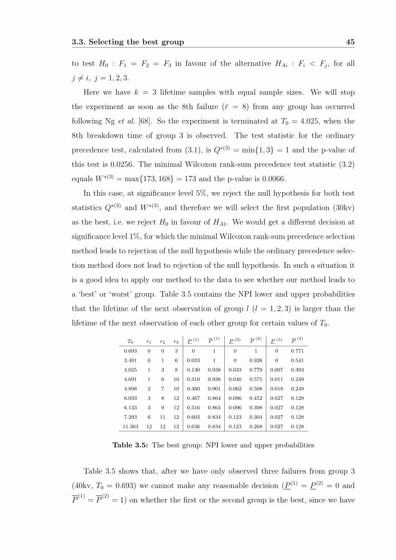
3.3. Selecting the best group 45
to test H0 : F1 = F2 = F3 in favour of the alternative HAi : Fi < Fj, for all
j 6= i, j = 1, 2, 3.
Here we have k = 3 lifetime samples with equal sample sizes. We will stop
the experiment as soon as the 8th failure (r = 8) from any group has occurred
following Ng et al. [68]. So the experiment is terminated at T0 = 4.025, when the
8th breakdown time of group 3 is observed. The test statistic for the ordinary
precedence test, calculated from (3.1), is Q∗(3) = min1, 3 = 1 and the p-value of
this test is 0.0256. The minimal Wilcoxon rank-sum precedence test statistic (3.2)
equals W ∗(3) = max173, 168 = 173 and the p-value is 0.0066.
In this case, at significance level 5%, we reject the null hypothesis for both test
statistics Q∗(3) and W ∗(3), and therefore we will select the first population (30kv)
as the best, i.e. we reject H0 in favour of HA1. We would get a different decision at
significance level 1%, for which the minimal Wilcoxon rank-sum precedence selection
method leads to rejection of the null hypothesis while the ordinary precedence selec-
tion method does not lead to rejection of the null hypothesis. In such a situation it
is a good idea to apply our method to the data to see whether our method leads to
a ‘best’ or ‘worst’ group. Table 3.5 contains the NPI lower and upper probabilities
that the lifetime of the next observation of group l (l = 1, 2, 3) is larger than the
lifetime of the next observation of each other group for certain values of T0.
T0 r1 r2 r3 P (1) P(1)
P (2) P(2)
P (3) P(3)
0.693 0 0 3 0 1 0 1 0 0.771
3.401 0 1 6 0.033 1 0 0.926 0 0.541
4.025 1 3 8 0.130 0.938 0.033 0.779 0.007 0.393
4.691 1 6 10 0.310 0.938 0.040 0.575 0.011 0.249
4.898 2 7 10 0.360 0.901 0.062 0.508 0.018 0.249
6.033 3 8 12 0.467 0.864 0.096 0.452 0.027 0.128
6.133 3 9 12 0.516 0.864 0.096 0.398 0.027 0.128
7.293 6 11 12 0.603 0.834 0.123 0.304 0.027 0.128
11.363 12 12 12 0.636 0.834 0.123 0.268 0.027 0.128
Table 3.5: The best group: NPI lower and upper probabilities
Table 3.5 shows that, after we have only observed three failures from group 3
(40kv, T0 = 0.693) we cannot make any reasonable decision (P (1) = P (2) = 0 and
P(1)
= P(2)
= 1) on whether the first or the second group is the best, since we have
3.4. Selecting the subset of best groups 46
not yet observed any failures from both groups.
However, at T0 = 4.025, when we have observed the 8th failure from group 3, we
have P (3) < P (2) < P (1) and P(3)
< P(2)
< P(1)
but P(3)
P (1) or P(3)
P (2). So,
there is no strong indication to select group 3 as the best group, which is in agreement
with the ordinary precedence test at significance level 1% that one particular group
is the worst. However, there is a weak indication that group 3 is the worst, but this
does not follow from the classical methods.
Here, when we have observed all failures, we have a strong indication that group
1 is the best as P(2)
< P (1) and P(3)
< P (1). In fact this holds already at T0 = 6.033.
At T0 = 4.691 we can conclude already that group 1 is better than group 3 as from
that moment on we have P(3)
< P (1). Then at T0 = 6.133, we also have in addition
P(2)
< P (1) and consequently we have a strong indication that group 1 is the best.
So at T0 = 4.025, our method leads to a conclusion in the line with the minimal
Wilcoxon rank-sum precedence selection method.
In this example we show that the NPI method and the classical precedence tests
do not necessarily lead to the same conclusions, but it is difficult to compare these
two due to the different inferential goals and the different basic underlying assump-
tions. Hence, we do not see these as competing methods for the same problems, but
more as complementary methods that can provide further insight into specific appli-
cations, and which may be more or less suitable depending on the explicit inferential
goal. 4
3.4 Selecting the subset of best groups
Suppose that the experiment is terminated at time T0 and our interest is to select
a subset of groups such that all the groups in this subset are ‘better’ than all not
selected groups, that is the lifetime of the next observation of each group in the
subset will be greater than the lifetime of the next observation of all groups not in
the subset. Let S = l1, l2, . . . , lm be a subset of m groups (1 ≤ m ≤ k− 1) from k
independent groups, and let NS be the complementary set of S which contains the
remaining k −m groups.
3.4. Selecting the subset of best groups 47
We will derive the NPI lower and upper probabilities for the event that the next
observation of each group in S has longer lifetime than the next observation of each
group in NS, denoted by
P S= P
(
minl∈S
Xl,nl+1 > maxj∈NS
Xj,nj+1
)
and PS= P
(
minl∈S
Xl,nl+1 > maxj∈NS
Xj,nj+1
)
These NPI lower and upper probabilities are given in Theorem 3.3, where the fol-
lowing notation is usedrl+2∑∑∑∑∑∑
il=1
l∈S
=
rl1+2∑
il1=1
...
rlm+2∑
ilm=1
(3.5)
Theorem 3.3. The NPI lower and upper probabilities for the event that the next
observation of each group in S has longer lifetime than the next observation of each
group in NS are
P S =
rl+2∑∑∑∑∑∑
il=1
l∈S
∏
j∈NS
∑rjij=1 1xj,ij < min
l∈SL(I lil)
nj + 1
.∏
l∈S
MXl,nl+1(I lil) (3.6)
PS=
rl+2∑∑∑∑∑∑
il=1
l∈S
∏
j∈NS
1 +∑rj
ij=1 1xj,ij < minl∈S
U(I lil)nj + 1
+
(nj − rj)1T0 < minl∈S
U(I lil)nj + 1
.∏
l∈S
MXl,nl+1(I lil) (3.7)
Proof. First, we derive the lower probability as follows
P
(
minl∈S
Xl,nl+1 > maxj∈NS
Xj,nj+1
)
= P
(
⋂
j∈NS
Xj,nj+1 < minl∈S
Xl,nl+1)
=
rl+2∑∑∑∑∑∑
il=1
l∈S
P
(
⋂
j∈NS
Xj,nj+1 < minl∈S
Xl,nl+1|Xl,nl+1 ∈ I lil , l ∈ S
)
.∏
l∈S
MXl,nl+1(I lil)
≥rl+2∑∑∑∑∑∑
il=1
l∈S
P
(
⋂
j∈NS
Xj,nj+1 < minl∈S
L(I lil))
.∏
l∈S
MXl,nl+1(I lil)
≥rl+2∑∑∑∑∑∑
il=1
l∈S
∏
j∈NS
∑rjij=1 1xj,ij < min
l∈SL(I lil)
nj + 1
.∏
l∈S
MXl,nl+1(I lil)
3.4. Selecting the subset of best groups 48
The first inequality follows by putting all probability mass for Xl,nl+1 (l ∈ S) as-
signed to the intervals I lil = (xl,il−1, xl,il) for il = 1, . . . , rl, (xl,rl ,∞) and (T0,∞)
in the left end points of these intervals, and by using Lemma 1.4 for the nested
intervals (xl,rl ,∞) and (T0,∞). The second inequality follows by putting all prob-
ability mass for Xj,nj+1 (j ∈ NS) assigned to the intervals Ijij = (xj,ij−1, xj,ij) for
ij = 1, . . . , rj, (xj,rj ,∞) and (T0,∞) in the right end points of these intervals. The
upper probability is obtained in a similar way, but now all probability masses for
the random quantities involved are put at the opposite end points of the respective
intervals, which leads to
P
(
minl∈S
Xl,nl+1 > maxj∈NS
Xj,nj+1
)
= P
(
⋂
j∈NS
Xj,nj+1 < minl∈S
Xl,nl+1)
=
rl+2∑∑∑∑∑∑
il=1
l∈S
P
(
⋂
j∈NS
Xj,nj+1 < minl∈S
Xl,nl+1|Xl,nl+1 ∈ I lil , l ∈ S
)
.∏
l∈S
MXl,nl+1(I lil)
≤rl+2∑∑∑∑∑∑
il=1
l∈S
P
(
⋂
j∈NS
Xj,nj+1 < minl∈S
U(I lil))
.∏
l∈S
MXl,nl+1(I lil)
≤rl+2∑∑∑∑∑∑
il=1
l∈S
∏
j∈NS
rj+2∑
ij=1
1L(Ijij) < minl∈S
U(I lil). MXj,nj+1(Ijij)
∏
l∈S
MXl,nl+1(I lil)
=
rl+2∑∑∑∑∑∑
il=1
l∈S
∏
j∈NS
1+∑rj
ij=11xj,ij<minl∈S
U(I lil)+(nj−rj)1T0<minl∈S
U(I lil)nj + 1
∏
l∈S
MXl,nl+1(I lil)
3.4.1 Special cases
We now present some special cases of the NPI lower and upper probabilities (3.6)
and (3.7).
1. If rl = 0 for all l ∈ S, then the NPI lower probability is
P S =∏
j∈NS
rjnj + 1
∏
l∈S
nl
nl + 1
and P S = 0 if there exists at least one j ∈ NS for which rj = 0. Since we
have not seen any failure from any group in S, this means that we cannot
3.4. Selecting the subset of best groups 49
exclude the possibility that we will never see a failure from any group in S,
consequently PS= 1.
2. If rj = 0 for at least one j ∈ NS and rl ≥ 0 for all l ∈ S, then the NPI lower
probability P S = 0 since there exists a group in NS for which we have not
seen any failure. This means that we cannot exclude the situation that we will
never see a failure from this group. Further, if rj = 0 for all j ∈ NS then the
NPI upper probability is
PS=∏
l∈S
nl − rl + 1
nl + 1
(
1−∏
j∈NS
1
nj + 1
)
+∏
j∈NS
1
nj + 1
3.4.2 Some properties
Now, we study the effect upon the lower and upper probabilities (3.6) and (3.7)
when the stopping time is increased from T0 to T0 + ε for small ε > 0, such that
there is only one extra failure from one group occurs.
Theorem 3.4. (i) If a failure from group l∗ ∈ S occurs in the interval (T0, T0 + ε),
then the NPI lower probability P S remains constant. However, the NPI upper
probability PSdecreases by
1
nl∗ + 1
∏
l∈S\l∗
nl − rl + 1
nl + 1
(
1−∏
j∈NS
rj + 1
nj + 1
)
except when rj = nj, for all j ∈ NS, in which case the upper probability remains
constant.
(ii) If a failure from group j∗ ∈ NS occurs in the interval (T0, T0 + ε), then the NPI
upper probability PSremains constant. However, the NPI lower probability P S
increases by1
nj∗ + 1
∏
j∈NS\j∗
rjnj + 1
∏
l∈S
nl − rlnl + 1
except when rl = nl for at least one l ∈ S or when there exists a j ∈ NS \ j∗ for
which rj = 0, in which cases the lower probability remains constant.
Proof. For case i (ii), replace rl∗ (rj∗) by rl∗ = rl+1 (rj∗ = rj∗+1) in formula (3.6)
and (3.7), then this follows by basic analysis of the lower and upper probabilities
3.4. Selecting the subset of best groups 50
of Theorem 3.3. For the sake of completeness we include the detailed proof below.
To reduce notation we use L∗(I lil)= minl∈S\l∗
L(I lil) and U∗(I lil)= minl∈S\l∗
U(I lil). First to
proof case (i),
P Sl∗ =
rl+2∑∑∑∑∑∑
il=1
l∈S\l∗
rl∗∑
il∗=1
∏
j∈NS
rj∑
ij=1
1xj,ij<minl∈S
L(I lil)(nj + 1)(nl∗ + 1)
+
∏
j∈NS
rj∑
ij=1
1xj,ij<minxl∗,rl∗ , L∗(I lil)
(nj + 1)(nl∗ + 1)+∏
j∈NS
rj∑
ij=1
1xj,ij<minxl∗,rl∗ , L∗(I lil)
(nj + 1)(nl∗ + 1)+
∏
j∈NS
rj∑
ij=1
1xj,ij<minT0+ε, L∗(I lil)(nl∗−rl∗−1)
(nj + 1)(nl∗ + 1)
∏
l∈S\l∗
MXl,nl+1(I lil)
= P S +
rl+2∑∑∑∑∑∑
il=1
l∈S\l∗
∏
j∈NS
rj∑
ij=1
1xj,ij < minxl∗,rl∗ , L∗(I lil)
(nj + 1)(nl∗ + 1)+
∏
j∈NS
rj∑
ij=1
1xj,ij < minT0 + ε, L∗(I lil)(nl∗ − rl∗ − 1)
(nj + 1)(nl∗ + 1)−
∏
j∈NS
rj∑
ij=1
1xj,ij < minT0, L∗(I lil)(nl∗ − rl∗)
(nj + 1)(nl∗ + 1)
∏
l∈S\l∗
MXl,nl+1(I lil)
And since for all l ∈ S \ l∗, 0 ≤ L(I lil) ≤ T0 < xl∗,rl∗ < T0 + ε, and consequently
minxl∗,rl∗ , L∗(I lil) = minT0 + ε, L∗(I lil) = minT0, L
∗(I lil) = L∗(I lil)
then the last term between square brackets will vanish. And,
PS
l∗ =
rl+2∑∑∑∑∑∑
il=1
l∈S\l∗
rl∗∑
il∗=1
∏
j∈NS
rj+2∑
ij=1
1L(Ijij)< minl∈S
U(I lil)MXj,nj+1(Ijij) +
∏
j∈NS
rj+2∑
ij=1
1L(Ijij) < minxl∗,rl∗ , U∗(I lil)
nl∗ + 1MXj,nj+1
(Ijij) +
∏
j∈NS
rj+2∑
ij=1
1L(Ijij)< minU(I l∗
rl∗+1), U∗(I lil)
nl∗ + 1MXj,nj+1
(Ijij) +
∏
j∈NS
rj+2∑
ij=1
1L(Ijij)<minU(I l∗
rl∗+2), U∗(I lil)(nl∗−rl∗−1)
nl∗ + 1MXj,nj+1
(Ijij)
.∏
l∈S\l∗
MXl,nl+1(I lil)
3.4. Selecting the subset of best groups 51
= PS+
1
nl∗+1
rl+2∑∑∑∑∑∑
il=1
l∈S\l∗
∏
j∈NS
rj+2∑
ij=1
1L(Ijij)< minxl∗,rl∗ , U∗(I lil)MXj,nj+1
(Ijij) −
∏
j∈NS
rj+2∑
ij=1
1L(Ijij)<U∗(I lil)MXj,nj+1(Ijij)
∏
l∈S\l∗
MXl,nl+1(I lil) (3.8)
Now,
rj+2∑
ij=1
1L(Ijij)<U∗(I lil)MXj,nj+1(Ijij)=
1+rj∑
ij=1
1xj,ij<U∗(I lil)+(nj−rj)1T0+ε<U∗(I lil)
nj + 1
(3.9)
and since 1T0 + ε < minxl∗,rl∗ , U∗(I lil) = 0 for l ∈ S \ l∗ and all il, we have
rj+2∑
ij=1
1L(Ijij)<minxl∗,rl∗,U∗(I lil)MXj,nj+1
(Ijij)=
1+rj∑
ij=1
1xj,ij<minxl∗,rl∗,U∗(I lil)
nj + 1
(3.10)
If U∗(I lil) 6= ∞, then (3.9) and (3.10) will be equal and consequently the term be-
tween square brackets in (3.8) will vanish. However, for U∗(I lil) = ∞, the equations
(3.9) and (3.10) reduce to 1 and (rj + 1)/(nj + 1), respectively. Therefore, we can
rewrite (3.8) as
PS
l∗ = PS+
1
nl∗ + 1
(
∏
j∈NS
rj + 1
nj + 1− 1
)
rl+2∑∑∑∑∑∑
il=rl+1
l∈S\l∗
∏
l∈S\l∗
MXl,nl+1(I lil)
= PS+
1
nl∗ + 1
(
∏
j∈NS
rj + 1
nj + 1− 1
)
∏
l∈S\l∗
rl+2∑∑∑∑∑∑
il=rl+1
l∈S\l∗
MXl,nl+1(I lil)
= PS+
1
nl∗ + 1
(
∏
j∈NS
rj + 1
nj + 1− 1
)
∏
l∈S\l∗
(
1
nl + 1+
nl − rlnl + 1
)
(3.11)
We used the known identity (∑
i ai)(∑
j bj) =∑
i
∑
j aibj to obtain the final form of
PS
l∗ , i.e. (3.11). And when rj = nj ∀j ∈ NS , it follows from (3.11) that PS
l∗ = PS
which completes the proof of part (i).
3.4. Selecting the subset of best groups 52
And for case (ii),
P Sj∗ =
rl+2∑∑∑∑∑∑
il=1
l∈S
∏
j∈NS\j∗
∑rjij=1 1xj,ij< min
l∈SL(I lil)
nj + 1
.
∑rj∗
ij∗=11xj∗,ij∗< minl∈S
L(I lil)+1xj∗,rj∗< minl∈S
L(I lil)nj∗ + 1
∏
l∈S
MXl,nl+1(I lil)
= P S +
rl+2∑∑∑∑∑∑
il=1
l∈S
∏
j∈NS\j∗
∑rjij=1 1xj,ij< min
l∈SL(I lil)
nj + 1
.
1xj∗,rj∗< minl∈S
L(I lil)nj∗ + 1
.∏
l∈S
MXl,nl+1(I lil) (3.12)
Since for all l ∈ S , xl,rl < xj∗,rj∗ < T0 + ε, we have 1xj∗,rj∗ < minl∈S
L(I lil) = 0
except when il = rl + 2, ∀l ∈ S, in which case L(I lil) = T0 + ε and therefore
1xj∗,rj∗ < T0 + ε = 1. Recall that when the experiment is terminated at xj∗,rj∗
(i.e. xj∗,rj∗ = T0 + ε), we assume that this stopping time is beyond xj∗,rj∗ by a very
small value which tends to zero. We can rewrite (3.12) as
P Sj∗ = P S +
1xj∗,rj∗ < T0 + εnj∗ + 1
∏
j∈NS\j∗
∑rjij=1 1xj,ij < T0 + ε
nj + 1
∏
l∈S
nl − rlnl + 1
= P S +1
nj∗ + 1
∏
j∈NS\j∗
rjnj + 1
∏
l∈S
nl − rlnl + 1
(3.13)
and indeed we see that the lower probability P Sj∗ is greater than or equal to P S.
From (3.13), it is clear that when there exists at least one l ∈ S for which rl = nl
then P Sj∗ = P S. Also P S
j∗ = P S when there exists a j ∈ NS \j∗ for which rj = 0.
PS
j∗ =
rl+2∑∑∑∑∑∑
il=1
l∈S
∏
j∈NS\j∗
1+∑rj
ij=11xj,ij<minl∈S
U(I lil)+(nj−rj)1T0 + ε<minl∈S
U(I lil)nj + 1
.
1+∑r∗j
ij∗=1 1xj∗,ij∗<minl∈S
U(I lil)nj∗ + 1
+1xj∗,rj∗<min
l∈SU(I lil)
nj∗ + 1+
(nj∗−rj∗−1)1T0 + ε<minl∈S
U(I lil)nj∗ + 1
∏
l∈S
MXl,nl+1(I lil) (3.14)
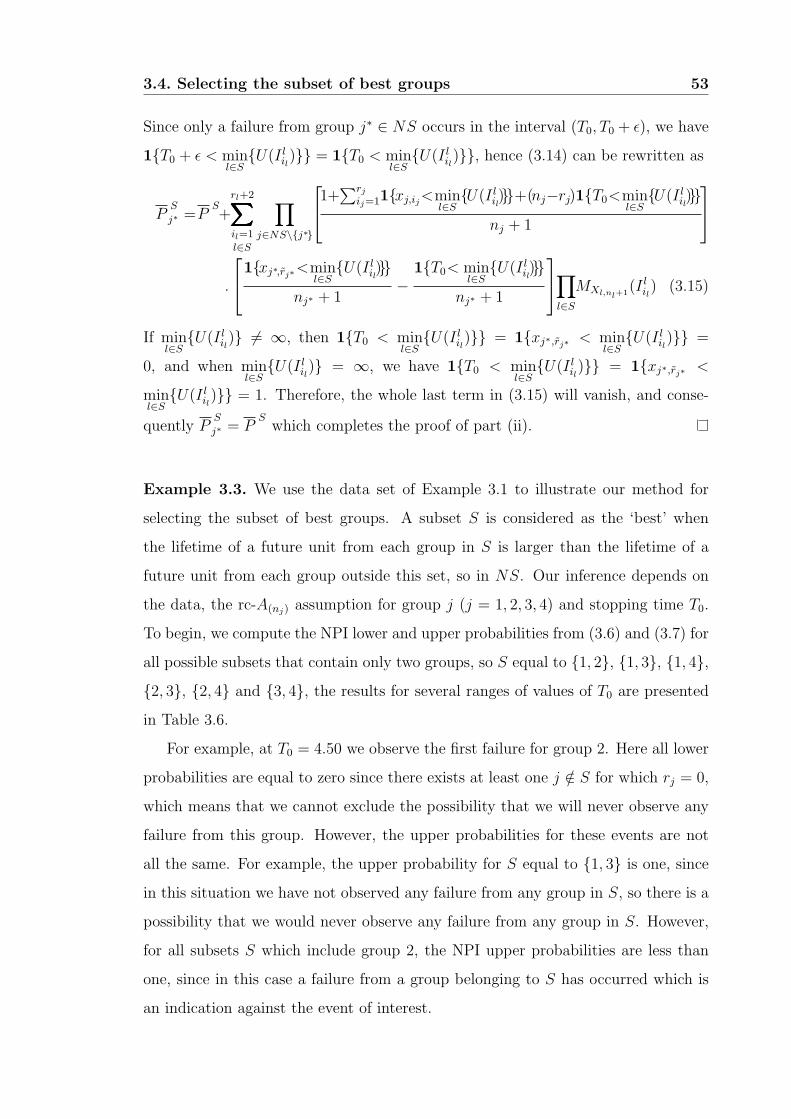
3.4. Selecting the subset of best groups 53
Since only a failure from group j∗ ∈ NS occurs in the interval (T0, T0 + ε), we have
1T0 + ε < minl∈S
U(I lil) = 1T0 < minl∈S
U(I lil), hence (3.14) can be rewritten as
PS
j∗ =PS+
rl+2∑∑∑∑∑∑
il=1
l∈S
∏
j∈NS\j∗
1+∑rj
ij=11xj,ij<minl∈S
U(I lil)+(nj−rj)1T0<minl∈S
U(I lil)nj + 1
.
1xj∗,rj∗<minl∈S
U(I lil)nj∗ + 1
−1T0< min
l∈SU(I lil)
nj∗ + 1
∏
l∈S
MXl,nl+1(I lil) (3.15)
If minl∈S
U(I lil) 6= ∞, then 1T0 < minl∈S
U(I lil) = 1xj∗,rj∗ < minl∈S
U(I lil) =
0, and when minl∈S
U(I lil) = ∞, we have 1T0 < minl∈S
U(I lil) = 1xj∗,rj∗ <
minl∈S
U(I lil) = 1. Therefore, the whole last term in (3.15) will vanish, and conse-
quently PS
j∗ = PSwhich completes the proof of part (ii).
Example 3.3. We use the data set of Example 3.1 to illustrate our method for
selecting the subset of best groups. A subset S is considered as the ‘best’ when
the lifetime of a future unit from each group in S is larger than the lifetime of a
future unit from each group outside this set, so in NS. Our inference depends on
the data, the rc-A(nj) assumption for group j (j = 1, 2, 3, 4) and stopping time T0.
To begin, we compute the NPI lower and upper probabilities from (3.6) and (3.7) for
all possible subsets that contain only two groups, so S equal to 1, 2, 1, 3, 1, 4,2, 3, 2, 4 and 3, 4, the results for several ranges of values of T0 are presented
in Table 3.6.
For example, at T0 = 4.50 we observe the first failure for group 2. Here all lower
probabilities are equal to zero since there exists at least one j /∈ S for which rj = 0,
which means that we cannot exclude the possibility that we will never observe any
failure from this group. However, the upper probabilities for these events are not
all the same. For example, the upper probability for S equal to 1, 3 is one, since
in this situation we have not observed any failure from any group in S, so there is a
possibility that we would never observe any failure from any group in S. However,
for all subsets S which include group 2, the NPI upper probabilities are less than
one, since in this case a failure from a group belonging to S has occurred which is
an indication against the event of interest.
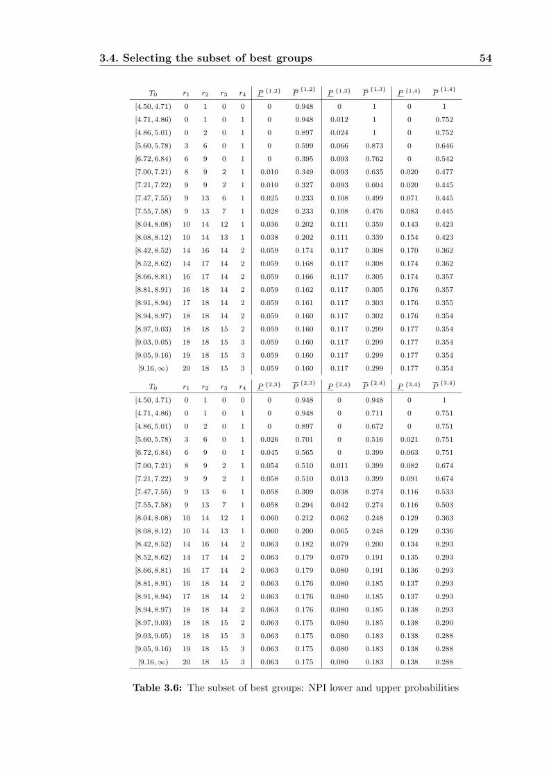
3.4. Selecting the subset of best groups 54
T0 r1 r2 r3 r4 P 1,2 P1,2
P 1,3 P1,3
P 1,4 P1,4
[4.50, 4.71) 0 1 0 0 0 0.948 0 1 0 1
[4.71, 4.86) 0 1 0 1 0 0.948 0.012 1 0 0.752
[4.86, 5.01) 0 2 0 1 0 0.897 0.024 1 0 0.752
[5.60, 5.78) 3 6 0 1 0 0.599 0.066 0.873 0 0.646
[6.72, 6.84) 6 9 0 1 0 0.395 0.093 0.762 0 0.542
[7.00, 7.21) 8 9 2 1 0.010 0.349 0.093 0.635 0.020 0.477
[7.21, 7.22) 9 9 2 1 0.010 0.327 0.093 0.604 0.020 0.445
[7.47, 7.55) 9 13 6 1 0.025 0.233 0.108 0.499 0.071 0.445
[7.55, 7.58) 9 13 7 1 0.028 0.233 0.108 0.476 0.083 0.445
[8.04, 8.08) 10 14 12 1 0.036 0.202 0.111 0.359 0.143 0.423
[8.08, 8.12) 10 14 13 1 0.038 0.202 0.111 0.339 0.154 0.423
[8.42, 8.52) 14 16 14 2 0.059 0.174 0.117 0.308 0.170 0.362
[8.52, 8.62) 14 17 14 2 0.059 0.168 0.117 0.308 0.174 0.362
[8.66, 8.81) 16 17 14 2 0.059 0.166 0.117 0.305 0.174 0.357
[8.81, 8.91) 16 18 14 2 0.059 0.162 0.117 0.305 0.176 0.357
[8.91, 8.94) 17 18 14 2 0.059 0.161 0.117 0.303 0.176 0.355
[8.94, 8.97) 18 18 14 2 0.059 0.160 0.117 0.302 0.176 0.354
[8.97, 9.03) 18 18 15 2 0.059 0.160 0.117 0.299 0.177 0.354
[9.03, 9.05) 18 18 15 3 0.059 0.160 0.117 0.299 0.177 0.354
[9.05, 9.16) 19 18 15 3 0.059 0.160 0.117 0.299 0.177 0.354
[9.16,∞) 20 18 15 3 0.059 0.160 0.117 0.299 0.177 0.354
T0 r1 r2 r3 r4 P 2,3 P2,3
P 2,4 P2,4
P 3,4 P3,4
[4.50, 4.71) 0 1 0 0 0 0.948 0 0.948 0 1
[4.71, 4.86) 0 1 0 1 0 0.948 0 0.711 0 0.751
[4.86, 5.01) 0 2 0 1 0 0.897 0 0.672 0 0.751
[5.60, 5.78) 3 6 0 1 0.026 0.701 0 0.516 0.021 0.751
[6.72, 6.84) 6 9 0 1 0.045 0.565 0 0.399 0.063 0.751
[7.00, 7.21) 8 9 2 1 0.054 0.510 0.011 0.399 0.082 0.674
[7.21, 7.22) 9 9 2 1 0.058 0.510 0.013 0.399 0.091 0.674
[7.47, 7.55) 9 13 6 1 0.058 0.309 0.038 0.274 0.116 0.533
[7.55, 7.58) 9 13 7 1 0.058 0.294 0.042 0.274 0.116 0.503
[8.04, 8.08) 10 14 12 1 0.060 0.212 0.062 0.248 0.129 0.363
[8.08, 8.12) 10 14 13 1 0.060 0.200 0.065 0.248 0.129 0.336
[8.42, 8.52) 14 16 14 2 0.063 0.182 0.079 0.200 0.134 0.293
[8.52, 8.62) 14 17 14 2 0.063 0.179 0.079 0.191 0.135 0.293
[8.66, 8.81) 16 17 14 2 0.063 0.179 0.080 0.191 0.136 0.293
[8.81, 8.91) 16 18 14 2 0.063 0.176 0.080 0.185 0.137 0.293
[8.91, 8.94) 17 18 14 2 0.063 0.176 0.080 0.185 0.137 0.293
[8.94, 8.97) 18 18 14 2 0.063 0.176 0.080 0.185 0.138 0.293
[8.97, 9.03) 18 18 15 2 0.063 0.175 0.080 0.185 0.138 0.290
[9.03, 9.05) 18 18 15 3 0.063 0.175 0.080 0.183 0.138 0.288
[9.05, 9.16) 19 18 15 3 0.063 0.175 0.080 0.183 0.138 0.288
[9.16,∞) 20 18 15 3 0.063 0.175 0.080 0.183 0.138 0.288
Table 3.6: The subset of best groups: NPI lower and upper probabilities
3.4. Selecting the subset of best groups 55
We can also study the behaviour of the NPI lower and upper probabilities when a
failure from any group occurs. To this end, assume that we terminate the experiment
at T0 = 7. In this situation we have observed 8, 9, 2 and 1 failures from groups 1,
2, 3 and 4, respectively. Suppose that we are interested in the subset S = 1, 2.In this case, P 1,2 = 0.010 and P
1,2= 0.349. Suppose now that the stopping
time is increased from 7 to 7.21. In this case a failure occurs from the first group
at time 7.21. We see that, while the lower probability remains constant, the upper
probability decreases from 0.349 to 0.327, which illustrates Theorem 3.4(i). However,
when increasing the stopping time from 8.04 to 8.08, so that an extra failure of group
3 occurs, the upper probability that S = 1, 2 is the subset with the best groups
remains constant, but the lower probability increases from 0.036 to 0.038, which
illustrates Theorem 3.4(ii).
Suppose now that we stop the experiment at T0 = 8.97 and that we are interested
in S = 2, 3. Then we have observed all units from all groups in S, but there are 3
units that still have not failed in groups in NS. For T0 ≥ 8.97, the lower and upper
probabilities that S = 2, 3 is the subset with the two best groups will not change
(P 2,3= 0.063, P2,3
= 0.175), which illustrates the special case of Theorem 3.4(ii).
If we change attention to S = 1, 4, also for T0 ≥ 8.97, then the lower and upper
probabilities again remain constant (P 1,4= 0.177, P1,4
= 0.354) since we have
observed all units from NS, which illustrates the special case of Theorem 3.4(i).
To carry out the comparison to select the best subset, we notice that if we
terminate the experiment at T0 = 8.52, P1,2
< P 1,4 which provides a strong
indicates to exclude 1, 2 from being the best. In addition, at T0 = 8.97 we can
exclude the set 2, 3 from being the subset with the best groups as P2,3
< P 1,4.
This may be due to the fact that the second group is included in these sets, since the
second group was the worse group as found in Example 3.1. However, this does not
hold for 2, 4 as P2,4
≯ P 1,4. This happens because this set consists of the best
and the worse group (see the results of Example 3.1). So, we only have a strong
indication that 1, 2 and 2, 3 are not the best subsets. As P 2,4 < P 1,3 <
P 3,4 < P 1,4 and P2,4
< P3,4
< P1,3
< P1,4
there is a weak indication
that S = 1, 4 is the best subset of size 2. 4
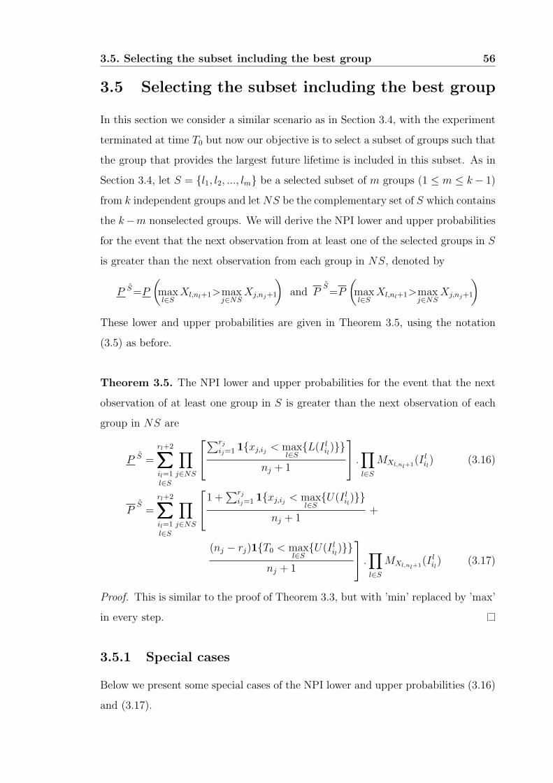
3.5. Selecting the subset including the best group 56
3.5 Selecting the subset including the best group
In this section we consider a similar scenario as in Section 3.4, with the experiment
terminated at time T0 but now our objective is to select a subset of groups such that
the group that provides the largest future lifetime is included in this subset. As in
Section 3.4, let S = l1, l2, ..., lm be a selected subset of m groups (1 ≤ m ≤ k− 1)
from k independent groups and letNS be the complementary set of S which contains
the k−m nonselected groups. We will derive the NPI lower and upper probabilities
for the event that the next observation from at least one of the selected groups in S
is greater than the next observation from each group in NS, denoted by
P S=P
(
maxl∈S
Xl,nl+1>maxj∈NS
Xj,nj+1
)
and PS=P
(
maxl∈S
Xl,nl+1>maxj∈NS
Xj,nj+1
)
These lower and upper probabilities are given in Theorem 3.5, using the notation
(3.5) as before.
Theorem 3.5. The NPI lower and upper probabilities for the event that the next
observation of at least one group in S is greater than the next observation of each
group in NS are
P S =
rl+2∑∑∑∑∑∑
il=1
l∈S
∏
j∈NS
∑rjij=1 1xj,ij < max
l∈SL(I lil)
nj + 1
.∏
l∈S
MXl,nl+1(I lil) (3.16)
PS=
rl+2∑∑∑∑∑∑
il=1
l∈S
∏
j∈NS
1 +∑rj
ij=1 1xj,ij < maxl∈S
U(I lil)nj + 1
+
(nj − rj)1T0 < maxl∈S
U(I lil)nj + 1
.∏
l∈S
MXl,nl+1(I lil) (3.17)
Proof. This is similar to the proof of Theorem 3.3, but with ’min’ replaced by ’max’
in every step.
3.5.1 Special cases
Below we present some special cases of the NPI lower and upper probabilities (3.16)
and (3.17).
3.5. Selecting the subset including the best group 57
1. If rl = 0 for at least one l ∈ S, then the NPI upper probability PS= 1, since
we have not seen any failure from at least one group in S. This means that
we cannot exclude the possibility that we would never see a failure from such
a group in S. Further, if rl = 0 for all l ∈ S, then the NPI lower probability is
P S =∏
j∈NS
rjnj + 1
(
1−∏
l∈S
1
nl + 1
)
which is equal to zero if there exists at least one j ∈ NS for which rj = 0.
2. If rj = 0 for at least one j ∈ NS and rl > 0 for all l ∈ S, then the NPI lower
probability P S = 0 since there exists a group in NS for which we have not
seen any failure. This means that we cannot exclude the possibility that we
would never see a failure from this group. Further, if rj = 0 for all j ∈ NS,
then the NPI upper probability is
PS= 1−
∏
l∈S
rlnl + 1
[
1−∏
j∈NS
1
nj + 1
]
so if rl = 0 for at least one l ∈ S, then PS= 1.
3.5.2 Some properties
Now, we study the effect upon the lower and upper probabilities when the stopping
time is increased from T0 to T0 + ε, for small ε > 0 such that only one extra failure
from one group occurs.
Theorem 3.6. (i) If a failure from group l∗ ∈ S occurs in the interval (T0, T0 + ε),
then the NPI lower probability P S remains constant, and the NPI upper probability
PSdecreases by
1
nl∗ + 1
∏
l∈S\l∗
rlnl + 1
(
1−∏
j∈NS
rj + 1
nj + 1
)
except when rj = nj for all j ∈ NS or when there exists a l ∈ S \ l∗ for which
rl = 0, in which cases the upper probability remains constant.
(ii) If a failure from group j∗ ∈ NS occurs in the interval (T0, T0 + ε), then the NPI
upper probability PSremains constant, and the NPI lower probability P S increases
3.5. Selecting the subset including the best group 58
by
1
nj∗ + 1
∏
j∈NS\j∗
rjnj + 1
(
1−∏
l∈S
rl + 1
nl + 1
)
except when rl = nl for all l ∈ S or when there exists a j ∈ NS \ j∗ for which
rj = 0, in which cases the lower probability remains constant.
Proof. For case i (ii), replace rl (rj∗) by rl + 1 (rj∗ + 1) in formula (3.16) and
(3.17), then this follows by basic analysis of the NPI lower and upper probabilities
of Theorem 3.5, see the proof of Theorem 3.4.
It can easily be shown that the NPI lower and upper probabilities for selecting the
subset of best groups, given by (3.6) and (3.7), cannot exceed those for selecting
the subset including the best group, given by (3.16) and (3.17). This follows from
1xj,ij < minl∈S
• ≤ 1xj,ij < maxl∈S
• and 1T0 < minl∈S
• ≤ 1T0 < maxl∈S
•,where ‘•’ refers to L(I lil) or U(I lil).
Example 3.4. Consider again the data set from Example 3.1, which we also used in
Example 3.3. The NPI lower and upper probabilities for the event that the lifetime
of the next observation from at least one group in S is greater than the lifetime
of the next observation of each group in NS, are calculated from (3.16) and (3.17)
at different stopping times T0 for all possible subsets containing 2 groups and are
presented in Table 3.7.
At T0 = 4.5, which is the moment when we observe the first failure (group 2),
all lower probabilities are zero and all upper probabilities are one, which is different
from the case when we select the subset of 2 best groups (Example 3.3), since for that
case there were some upper probabilities which are less than one. This is because at
T0 = 4.5, whichever subset of 2 groups we consider, this subset will always contain
at least one group for which we have not seen any failure, so there is no evidence
against the possibility that this subset can still contain the best group.
For example, for S = 1, 3, the lower probability at T0 = 4.71 is 0.013, while
the corresponding upper probability is one. At T0 = 4.71 we have seen failures from
groups 2 and 4. Therefore, we cannot exclude the possibility that we will not observe
any failure from any group in S. In fact, the upper probabilities for the sets that
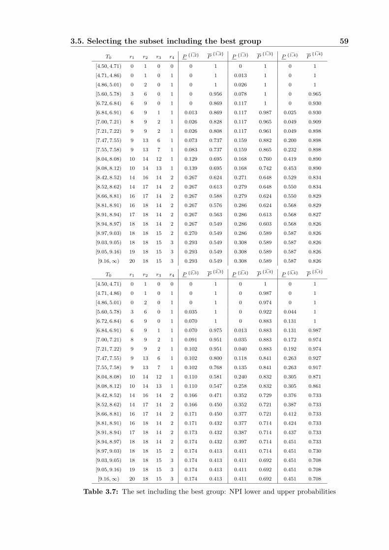
3.5. Selecting the subset including the best group 59
T0 r1 r2 r3 r4 P 1,2 P1,2
P 1,3 P1,3
P 1,4 P1,4
[4.50, 4.71) 0 1 0 0 0 1 0 1 0 1
[4.71, 4.86) 0 1 0 1 0 1 0.013 1 0 1
[4.86, 5.01) 0 2 0 1 0 1 0.026 1 0 1
[5.60, 5.78) 3 6 0 1 0 0.956 0.078 1 0 0.965
[6.72, 6.84) 6 9 0 1 0 0.869 0.117 1 0 0.930
[6.84, 6.91) 6 9 1 1 0.013 0.869 0.117 0.987 0.025 0.930
[7.00, 7.21) 8 9 2 1 0.026 0.828 0.117 0.965 0.049 0.909
[7.21, 7.22) 9 9 2 1 0.026 0.808 0.117 0.961 0.049 0.898
[7.47, 7.55) 9 13 6 1 0.073 0.737 0.159 0.882 0.200 0.898
[7.55, 7.58) 9 13 7 1 0.083 0.737 0.159 0.865 0.232 0.898
[8.04, 8.08) 10 14 12 1 0.129 0.695 0.168 0.760 0.419 0.890
[8.08, 8.12) 10 14 13 1 0.139 0.695 0.168 0.742 0.453 0.890
[8.42, 8.52) 14 16 14 2 0.267 0.624 0.271 0.648 0.529 0.834
[8.52, 8.62) 14 17 14 2 0.267 0.613 0.279 0.648 0.550 0.834
[8.66, 8.81) 16 17 14 2 0.267 0.588 0.279 0.624 0.550 0.829
[8.81, 8.91) 16 18 14 2 0.267 0.576 0.286 0.624 0.568 0.829
[8.91, 8.94) 17 18 14 2 0.267 0.563 0.286 0.613 0.568 0.827
[8.94, 8.97) 18 18 14 2 0.267 0.549 0.286 0.603 0.568 0.826
[8.97, 9.03) 18 18 15 2 0.270 0.549 0.286 0.589 0.587 0.826
[9.03, 9.05) 18 18 15 3 0.293 0.549 0.308 0.589 0.587 0.826
[9.05, 9.16) 19 18 15 3 0.293 0.549 0.308 0.589 0.587 0.826
[9.16,∞) 20 18 15 3 0.293 0.549 0.308 0.589 0.587 0.826
T0 r1 r2 r3 r4 P 2,3 P2,3
P 2,4 P2,4
P 3,4 P3,4
[4.50, 4.71) 0 1 0 0 0 1 0 1 0 1
[4.71, 4.86) 0 1 0 1 0 1 0 0.987 0 1
[4.86, 5.01) 0 2 0 1 0 1 0 0.974 0 1
[5.60, 5.78) 3 6 0 1 0.035 1 0 0.922 0.044 1
[6.72, 6.84) 6 9 0 1 0.070 1 0 0.883 0.131 1
[6.84, 6.91) 6 9 1 1 0.070 0.975 0.013 0.883 0.131 0.987
[7.00, 7.21) 8 9 2 1 0.091 0.951 0.035 0.883 0.172 0.974
[7.21, 7.22) 9 9 2 1 0.102 0.951 0.040 0.883 0.192 0.974
[7.47, 7.55) 9 13 6 1 0.102 0.800 0.118 0.841 0.263 0.927
[7.55, 7.58) 9 13 7 1 0.102 0.768 0.135 0.841 0.263 0.917
[8.04, 8.08) 10 14 12 1 0.110 0.581 0.240 0.832 0.305 0.871
[8.08, 8.12) 10 14 13 1 0.110 0.547 0.258 0.832 0.305 0.861
[8.42, 8.52) 14 16 14 2 0.166 0.471 0.352 0.729 0.376 0.733
[8.52, 8.62) 14 17 14 2 0.166 0.450 0.352 0.721 0.387 0.733
[8.66, 8.81) 16 17 14 2 0.171 0.450 0.377 0.721 0.412 0.733
[8.81, 8.91) 16 18 14 2 0.171 0.432 0.377 0.714 0.424 0.733
[8.91, 8.94) 17 18 14 2 0.173 0.432 0.387 0.714 0.437 0.733
[8.94, 8.97) 18 18 14 2 0.174 0.432 0.397 0.714 0.451 0.733
[8.97, 9.03) 18 18 15 2 0.174 0.413 0.411 0.714 0.451 0.730
[9.03, 9.05) 18 18 15 3 0.174 0.413 0.411 0.692 0.451 0.708
[9.05, 9.16) 19 18 15 3 0.174 0.413 0.411 0.692 0.451 0.708
[9.16,∞) 20 18 15 3 0.174 0.413 0.411 0.692 0.451 0.708
Table 3.7: The set including the best group: NPI lower and upper probabilities
3.5. Selecting the subset including the best group 60
contain group 3, i.e. 1, 3, 2, 3 and 3, 4, will be one until T0 = 6.84 (i.e. the
time at which we observe the first failure from group 3). The lower probabilities for
the sets that do not include the third group, i.e. 1, 2, 1, 4 and 2, 4, are zero
until T0 = 6.84.
To study the behaviour of these NPI lower and upper probabilities, let us consider
the situation when the stopping time T0 is increased from 7 to 7.21, and let S = 1, 2be the set of interest. At time 7.21 a failure of group 1 is observed. Here, the lower
probability remains constant as the amount of information in favour of this event
remains the same. However, the upper probability decreases from 0.828 to 0.808 as
the amount of information against this event has increased (Theorem 3.6(i)). When
we consider S = 2, 3, with T0 increasing from 7 to 7.21, then the upper probability
remains constant, but, the lower probability increases from 0.091 to 0.102, as the
amount of information in favour of this event now increases (Theorem 3.6(ii)).
At T0 = 8.97 we have observed failures of all units from groups 2 and 3. If the
set of interest is S = 2, 3, we see that the lower and upper probabilities remain
constant for T0 ≥ 8.97 since we have observed all units of all groups in S (special
case Theorem 3.6(ii)). Also, if the set of interest is S = 1, 4, the lower and upper
probabilities remain constant since we have observed all units from all groups in NS
(special case Theorem 3.6(i)).
At the time when we have observed all units from all groups, i.e. T0 = 9.16, we
have a strong indication that the set 1, 4 is better than 1, 2 and 2, 3, in the
sense that it is more likely that 1, 4 contains the best group since
0.549 = P1,2
< P 1,4 = 0.587 and 0.413 = P2,3
< P 1,4 = 0.587
In fact the set 1, 4 has the highest lower and upper probability when all failure
times have been observed for all units from all groups. However, we have a weak
indication that 1, 4 is the set which contains the best group since we have
P 1,3 < P 2,4 < P 3,4 < P 1,4 < P1,3
< P2,4
< P3,4
< P1,4
We can exclude 2, 3 from the comparison from T0 = 8.42 onwards, since P2,3
<
P 1,4. Also the set 1, 2 can be excluded from T0 = 8.91 onwards since P1,2
<
P 1,4. 4
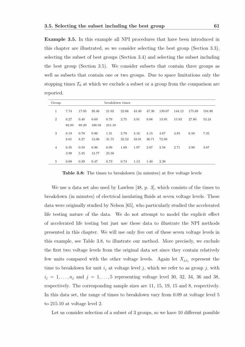
3.5. Selecting the subset including the best group 61
Example 3.5. In this example all NPI procedures that have been introduced in
this chapter are illustrated, so we consider selecting the best group (Section 3.3),
selecting the subset of best groups (Section 3.4) and selecting the subset including
the best group (Section 3.5). We consider subsets that contain three groups as
well as subsets that contain one or two groups. Due to space limitations only the
stopping times T0 at which we exclude a subset or a group from the comparison are
reported.
Group breakdown times
1 7.74 17.05 20.46 21.02 22.66 43.40 47.30 139.07 144.12 175.88 194.90
2 0.27 0.40 0.69 0.79 2.75 3.91 9.88 13.95 15.93 27.80 53.24
82.85 89.29 100.58 215.10
3 0.19 0.78 0.96 1.31 2.78 3.16 4.15 4.67 4.85 6.50 7.35
8.01 8.27 12.06 31.75 32.52 33.91 36.71 72.89
4 0.35 0.59 0.96 0.99 1.69 1.97 2.07 2.58 2.71 2.90 3.67
3.99 5.35 13.77 25.50
5 0.09 0.39 0.47 0.73 0.74 1.13 1.40 2.38
Table 3.8: The times to breakdown (in minutes) at five voltage levels
We use a data set also used by Lawless [48, p. 3], which consists of the times to
breakdown (in minutes) of electrical insulating fluids at seven voltage levels. These
data were originally studied by Nelson [65], who particularly studied the accelerated
life testing nature of the data. We do not attempt to model the explicit effect
of accelerated life testing but just use these data to illustrate the NPI methods
presented in this chapter. We will use only five out of these seven voltage levels in
this example, see Table 3.8, to illustrate our method. More precisely, we exclude
the first two voltage levels from the original data set since they contain relatively
few units compared with the other voltage levels. Again let Xj,ij represent the
time to breakdown for unit ij at voltage level j, which we refer to as group j, with
ij = 1, . . . , nj and j = 1, . . . , 5 representing voltage level 30, 32, 34, 36 and 38,
respectively. The corresponding sample sizes are 11, 15, 19, 15 and 8, respectively.
In this data set, the range of times to breakdown vary from 0.09 at voltage level 5
to 215.10 at voltage level 2.
Let us consider selection of a subset of 3 groups, so we have 10 different possible
3.5. Selecting the subset including the best group 62
subsets: 1, 2, 3, 1, 2, 4, 1, 2, 5, 1, 3, 4, 1, 3, 5, 1, 4, 5, 2, 3, 4, 2, 3, 5,2, 4, 5 and 3, 4, 5. Of course, there are also 10 possible subsets containing 2
different voltage levels: 1, 2, 1, 3, 1, 4, 1, 5, 2, 3, 2, 4, 2, 5, 3, 4,3, 5 and 4, 5.
We start considering selection of the subset of 3 best groups. When we have
observed all units from all groups we will select the subset 1, 2, 3 as the subset of
best groups with NPI lower and upper probabilities P 1,2,3 = 0.337 and P1,2,3
=
0.535, respectively. Actually we can conclude the same result (i.e. 1, 2, 3 as the
best subset) at an early stage. In fact, already if we stopped the experiment at
T0 = 6.5 we would select the set 1, 2, 3 as the best subset among all ten subsets,
see Table 3.9. Note that, at this point we still have not observed any breakdown
from the first group while we have observed already the breakdown times of all
units from group 5. Table 3.9 explains how we can establish an early decision from
the beginning. For example, at T0 = 2.38, we have observed all breakdown times
for units from group 5 and we have not observed any breakdowns from the first
group, and therefore we will exclude any set that contains group 5 from being the
best. Moreover, at T0 = 2.90 we can exclude 7 of the 10 subsets from comparison of
becoming the best subset. At this time, the subsets 1, 2, 3, 1, 2, 4 and 1, 3, 4remain in the comparison process. Figure 3.1 shows a pairwise comparison between
the best subset 1, 2, 3 and the two second best subsets 1, 2, 4 and 1, 3, 4, fordifferent T0. We can see that at T0 = 3.99, P
1,2,4< P 1,2,3 and at T0 = 6.50,
P1,3,4
< P 1,2,3.
Consequently, if we terminate the experiment at T0 = 6.5 we get the same
decision as when we would have observed all units from all groups. Doing that
would lead to a much shorter testing time, and we can keep 9 units out of 15 from
group 2, 9 out of 19 from group 3, 2 out of 15 from group 4 and all units from group
1 to be possibly used for other purposes.
Now we consider selecting a subset of 3 groups that includes the best group.
Table 3.10 shows that 4 out of 10 subsets could be excluded from the comparison at
T0 = 13.77, and a fifth subsets at T0 = 25.5. Unlike the case of selecting the subset
of best groups, there are three sets 1, 2, 3, 1, 2, 4 and 1, 2, 5 which cannot be
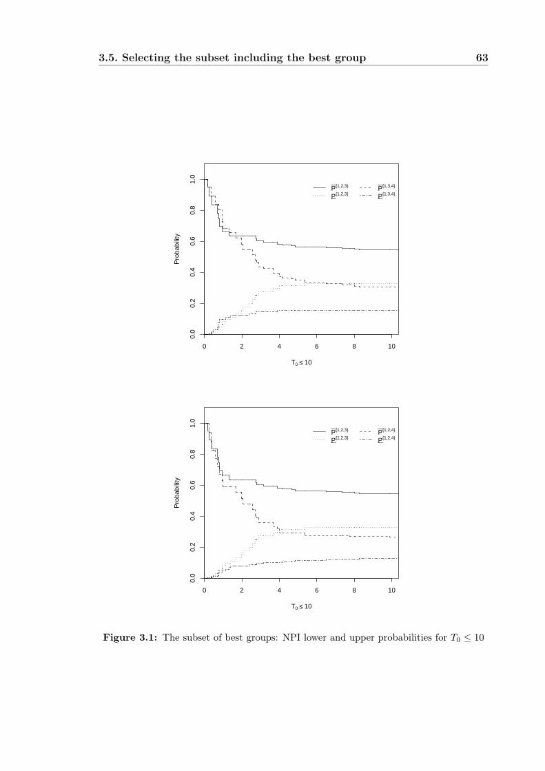
3.5. Selecting the subset including the best group 63
0 2 4 6 8 10
0.0
0.2
0.4
0.6
0.8
1.0
T0 ≤ 10
Pro
babi
lity
P1,2,3
P1,2,3P1,3,4
P1,3,4
0 2 4 6 8 10
0.0
0.2
0.4
0.6
0.8
1.0
T0 ≤ 10
Pro
babi
lity
P1,2,3
P1,2,3P1,2,4
P1,2,4
Figure 3.1: The subset of best groups: NPI lower and upper probabilities for T0 ≤ 10
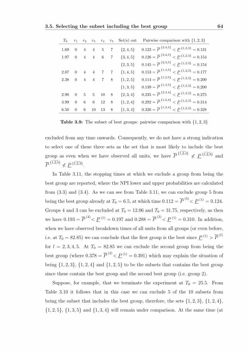
3.5. Selecting the subset including the best group 64
T0 r1 r2 r3 r4 r5 Set(s) out Pairwise comparison with 1, 2, 3
1.69 0 4 4 5 7 2, 4, 5 0.123 = P2,4,5
< P 1,2,3 = 0.131
1.97 0 4 4 6 7 3, 4, 5 0.126 = P3,4,5
< P 1,2,3 = 0.154
2, 3, 5 0.145 = P2,3,5
< P 1,2,3 = 0.154
2.07 0 4 4 7 7 1, 4, 5 0.153 = P1,4,5
< P 1,2,3 = 0.177
2.38 0 4 4 7 8 1, 2, 5 0.114 = P1,2,5
< P 1,2,3 = 0.200
1, 3, 5 0.139 = P1,3,5
< P 1,2,3 = 0.200
2.90 0 5 5 10 8 2, 3, 4 0.235 = P2,3,4
< P 1,2,3 = 0.275
3.99 0 6 6 12 8 1, 2, 4 0.292 = P1,2,4
< P 1,2,3 = 0.314
6.50 0 6 10 13 8 1, 3, 4 0.326 = P1,3,4
< P 1,2,3 = 0.328
Table 3.9: The subset of best groups: pairwise comparison with 1, 2, 3
excluded from any time onwards. Consequently, we do not have a strong indication
to select one of these three sets as the set that is most likely to include the best
group as even when we have observed all units, we have P1,2,4
≮ P 1,2,3 and
P1,2,5
≮ P 1,2,3.
In Table 3.11, the stopping times at which we exclude a group from being the
best group are reported, where the NPI lower and upper probabilities are calculated
from (3.3) and (3.4). As we can see from Table 3.11, we can exclude group 5 from
being the best group already at T0 = 6.5, at which time 0.112 = P(5)< P (1) = 0.124.
Groups 4 and 3 can be excluded at T0 = 12.06 and T0 = 31.75, respectively, as then
we have 0.193 = P(4)< P (1) = 0.197 and 0.288 = P
(3)< P (1) = 0.310. In addition,
when we have observed breakdown times of all units from all groups (or even before,
i.e. at T0 = 82.85) we can conclude that the first group is the best since P (1) > P(l)
for l = 2, 3, 4, 5. At T0 = 82.85 we can exclude the second group from being the
best group (where 0.378 = P(2)< P (1) = 0.391) which may explain the situation of
being 1, 2, 3, 1, 2, 4 and 1, 2, 5 to be the subsets that contains the best group
since these contain the best group and the second best group (i.e. group 2).
Suppose, for example, that we terminate the experiment at T0 = 25.5. From
Table 3.10 it follows that in this case we can exclude 5 of the 10 subsets from
being the subset that includes the best group, therefore, the sets 1, 2, 3, 1, 2, 4,1, 2, 5, 1, 3, 5 and 1, 3, 4 will remain under comparison. At the same time (at
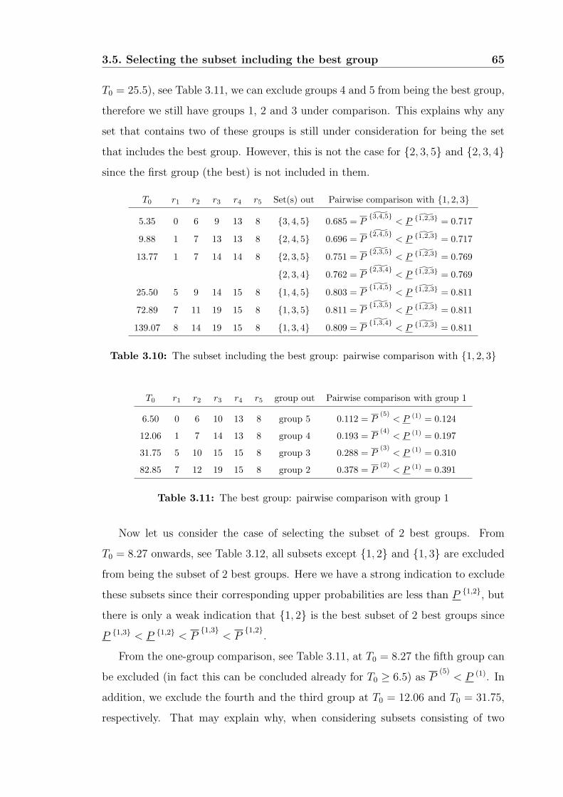
3.5. Selecting the subset including the best group 65
T0 = 25.5), see Table 3.11, we can exclude groups 4 and 5 from being the best group,
therefore we still have groups 1, 2 and 3 under comparison. This explains why any
set that contains two of these groups is still under consideration for being the set
that includes the best group. However, this is not the case for 2, 3, 5 and 2, 3, 4since the first group (the best) is not included in them.
T0 r1 r2 r3 r4 r5 Set(s) out Pairwise comparison with 1, 2, 3
5.35 0 6 9 13 8 3, 4, 5 0.685 = P3,4,5
< P 1,2,3 = 0.717
9.88 1 7 13 13 8 2, 4, 5 0.696 = P2,4,5
< P 1,2,3 = 0.717
13.77 1 7 14 14 8 2, 3, 5 0.751 = P2,3,5
< P 1,2,3 = 0.769
2, 3, 4 0.762 = P2,3,4
< P 1,2,3 = 0.769
25.50 5 9 14 15 8 1, 4, 5 0.803 = P1,4,5
< P 1,2,3 = 0.811
72.89 7 11 19 15 8 1, 3, 5 0.811 = P1,3,5
< P 1,2,3 = 0.811
139.07 8 14 19 15 8 1, 3, 4 0.809 = P1,3,4
< P 1,2,3 = 0.811
Table 3.10: The subset including the best group: pairwise comparison with 1, 2, 3
T0 r1 r2 r3 r4 r5 group out Pairwise comparison with group 1
6.50 0 6 10 13 8 group 5 0.112 = P(5)
< P (1) = 0.124
12.06 1 7 14 13 8 group 4 0.193 = P(4)
< P (1) = 0.197
31.75 5 10 15 15 8 group 3 0.288 = P(3)
< P (1) = 0.310
82.85 7 12 19 15 8 group 2 0.378 = P(2)
< P (1) = 0.391
Table 3.11: The best group: pairwise comparison with group 1
Now let us consider the case of selecting the subset of 2 best groups. From
T0 = 8.27 onwards, see Table 3.12, all subsets except 1, 2 and 1, 3 are excluded
from being the subset of 2 best groups. Here we have a strong indication to exclude
these subsets since their corresponding upper probabilities are less than P 1,2, but
there is only a weak indication that 1, 2 is the best subset of 2 best groups since
P 1,3 < P 1,2 < P1,3
< P1,2
.
From the one-group comparison, see Table 3.11, at T0 = 8.27 the fifth group can
be excluded (in fact this can be concluded already for T0 ≥ 6.5) as P(5)
< P (1). In
addition, we exclude the fourth and the third group at T0 = 12.06 and T0 = 31.75,
respectively. That may explain why, when considering subsets consisting of two
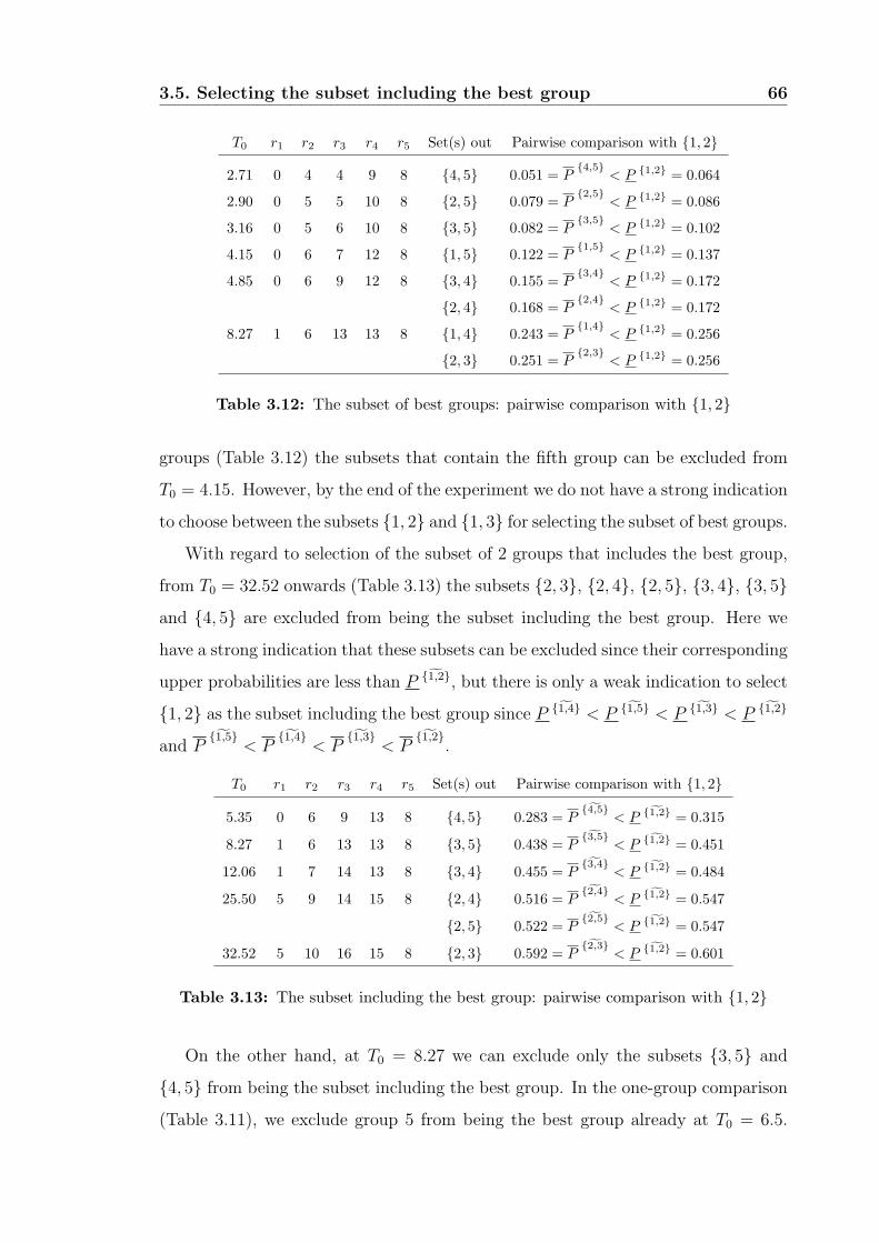
3.5. Selecting the subset including the best group 66
T0 r1 r2 r3 r4 r5 Set(s) out Pairwise comparison with 1, 2
2.71 0 4 4 9 8 4, 5 0.051 = P4,5
< P 1,2 = 0.064
2.90 0 5 5 10 8 2, 5 0.079 = P2,5
< P 1,2 = 0.086
3.16 0 5 6 10 8 3, 5 0.082 = P3,5
< P 1,2 = 0.102
4.15 0 6 7 12 8 1, 5 0.122 = P1,5
< P 1,2 = 0.137
4.85 0 6 9 12 8 3, 4 0.155 = P3,4
< P 1,2 = 0.172
2, 4 0.168 = P2,4
< P 1,2 = 0.172
8.27 1 6 13 13 8 1, 4 0.243 = P1,4
< P 1,2 = 0.256
2, 3 0.251 = P2,3
< P 1,2 = 0.256
Table 3.12: The subset of best groups: pairwise comparison with 1, 2
groups (Table 3.12) the subsets that contain the fifth group can be excluded from
T0 = 4.15. However, by the end of the experiment we do not have a strong indication
to choose between the subsets 1, 2 and 1, 3 for selecting the subset of best groups.With regard to selection of the subset of 2 groups that includes the best group,
from T0 = 32.52 onwards (Table 3.13) the subsets 2, 3, 2, 4, 2, 5, 3, 4, 3, 5and 4, 5 are excluded from being the subset including the best group. Here we
have a strong indication that these subsets can be excluded since their corresponding
upper probabilities are less than P 1,2, but there is only a weak indication to select
1, 2 as the subset including the best group since P 1,4 < P 1,5 < P 1,3 < P 1,2
and P1,5
< P1,4
< P1,3
< P1,2
.
T0 r1 r2 r3 r4 r5 Set(s) out Pairwise comparison with 1, 2
5.35 0 6 9 13 8 4, 5 0.283 = P4,5
< P 1,2 = 0.315
8.27 1 6 13 13 8 3, 5 0.438 = P3,5
< P 1,2 = 0.451
12.06 1 7 14 13 8 3, 4 0.455 = P3,4
< P 1,2 = 0.484
25.50 5 9 14 15 8 2, 4 0.516 = P2,4
< P 1,2 = 0.547
2, 5 0.522 = P2,5
< P 1,2 = 0.547
32.52 5 10 16 15 8 2, 3 0.592 = P2,3
< P 1,2 = 0.601
Table 3.13: The subset including the best group: pairwise comparison with 1, 2
On the other hand, at T0 = 8.27 we can exclude only the subsets 3, 5 and
4, 5 from being the subset including the best group. In the one-group comparison
(Table 3.11), we exclude group 5 from being the best group already at T0 = 6.5.
3.5. Selecting the subset including the best group 67
However, while 2, 5 contains the fifth group, it is still under comparison until
T0 = 25.5. With respect to 1, 5, and by the end of the experiment, there is no
strong indication to exclude this subset from being the subset including the best
group although this subset includes the best (group 1) and the worst group (group
5). Note that this subset was excluded at T0 = 4.15 from being the subset of 2 best
groups (Table 3.12). Actually we excluded all subsets that contain the fifth group
from being the subset of best groups at T0 = 4.15, which is even before we would
decide to exclude the fifth group from being the best group (one-group comparison,
Table 3.11) at T0 = 6.5.
At T0 = 6.5, we see from Table 3.9 that we can select 1, 2, 3 as the subset
of best groups containing 3 groups. However, at this time, we see from Table 3.12
that we do not have a strong indication to select one subset for being the subset of
best groups among 1, 2, 1, 3, 1, 4 and 2, 3, although 1, 2, 1, 3 and 2, 3are subsets of 1, 2, 3, but the subset 1, 4 contains only one group from 1, 2, 3.Later, at T0 = 8.27 we exclude the subset 2, 3 (⊂ 1, 2, 3) from being the subset
of best groups.
At T0 = 25.5, see Table 3.10, we do not have a strong indication to select one
of 1, 2, 3, 1, 2, 4, 1, 2, 5, 1, 3, 4 and 1, 3, 5 as the subset including the best
group. Here all possible 3-group subsets which include the best group (i.e. group 1)
are still under comparison except for 1, 4, 5, which contains the two worst groups
(i.e. groups 4 and 5) according to Table 3.11. However, we exclude the subset
1, 4, 5, at T0 = 25.5 from being the subset including the best group. However at
this time (Table 3.13) we do not have a strong indication in favour of selecting one
of 1, 2, 1, 3, 1, 4, 1, 5 and 2, 3 as the subset including the best group.
At T0 = 25.5, the subset 2, 3 is also still under comparison for being the subset
including the best group while group 1 (the best group) is not included in this
subset. However, at least all subsets that include group 1 (the best group) are still
under comparison for the subset including the best group when breakdown times
have been observed for all units on test. 4
3.6. Concluding remarks 68
3.6 Concluding remarks
In this chapter we have presented NPI for comparison of several groups through
experiments that may be terminated before the event of interest has been observed
for all units. This work generalizes the NPI approach for selection presented by
Coolen and van der Laan [25], with close links to methods for precedence testing
which are explicitly developed to deal with such early termination.
We note that when the stopping time increases from T0 to T0 + ε such that only
one extra failure occurs from one particular group, the lower probability remains ei-
ther constant or increases and the upper probability remains constant or decreases.
Hence, when T0 increases to T0 + ε, the imprecision remains constant or decreases.
It is shown that the lower probability for a certain event can be interpreted as quan-
tifying the amount of information in favour of the event while the upper probability
can be interpreted as quantifying the amount of information against the event.
The NPI method presented here is not considered to be a competitor for es-
tablished classical methods for precedence testing and selection, but it provides an
interesting alternative which may be suitable particularly in cases where interest is
explicitly in a future observation from one or more selected groups. It may well
be the case that these different methods lead to quite different conclusions, so care
must be taken about the actual inferential conclusions. As always, applying a variety
of suitable statistical methods to a practical problem might give valuable insights
into the problem and the different methods, where differences typically occur due
to different underlying assumptions and explicitly different inferential goals of the
methods.
Chapter 4
Comparisons of lifetime data with
early termination
4.1 Introduction
Coolen and Yan [26] introduced NPI for comparison of two groups of lifetime data
that contain right-censored observations, using the suitable rc-A(n) assumption per
group. However, they did not consider situations with more than two groups, nor
the effect of early termination of the lifetime experiment. In Chapters 2 and 3
we presented NPI for comparison of groups of data with early termination of the
experiment, say at time T0, but all observations prior to T0 were required to be actual
failure times, so no right-censoring was possible apart from the right-censoring at T0
of all units that had not yet failed. In this chapter we generalise that by developing
NPI for comparison of multiple groups of lifetime data including right-censored
observations, and with possible early termination of the lifetime experiment.
A short overview about the classical precedence tests is given in Section 4.2. The
NPI lower and upper probabilities for comparing k groups in order to select the best
group, with possible early termination of the lifetime experiment, are presented in
Section 4.3, and this approach is illustrated and discussed via examples in Section
4.4. Some concluding remarks are given in Section 4.5.
69
4.2. Classical precedence tests 70
4.2 Classical precedence tests
Suppose we have k ≥ 2 independent groups, for group j (j = 1, . . . , k) nj units are
placed on a lifetime experiment, and let their random times to failure be denoted
by Xj,1, . . . , Xj,nj. In classical statistics, it is typically assumed that these random
quantities are independent and identically distributed, with continuous distribution
function Fj. Several nonparametric tests have been proposed in the literature for
comparing k groups of units placed simultaneously on a lifetime experiment [15, 16].
Classical precedence testing methods consider the null hypothesis H0 : F1(x) =
. . . = Fk(x) for all x, which is tested against several alternative hypotheses, e.g. the
most general alternative H1 : Fi(x) 6= Fj(x) for at least one pair of i and j and
some value of x. Another alternative hypothesis that has been used is the one-sided
alternative H2 : Fi(x) ≤ F1(x), with strict inequality for at least one i = 2, 3, . . . , k
and some x [16]. This is of particular use in applications where one wants to com-
pare a control population, with distribution function F1, to other populations, with
distribution functions F2, . . . , Fk, to test if any of the other populations are better
than the control population. Tests for several alternative hypotheses are presented
in [15, 16]. For given p ∈ (0, 1), these tests typically depend on the statistics
Ujp = njFjF−11 (p), j = 2, 3, . . . , k, where Fj denotes the Kaplan-Meier estimator of
Fj(x) [44] and F−11 (u) is the Kaplan-Meier quantile function corresponding to F1.
The asymptotic distribution of some functions of these statistics Ujp are given in
[16], which also presents more details of such nonparametric precedence tests.
Let us consider one of these precedence tests proposed by Chakraborti and Desu
[15] where, for a test of size α, one may reject H0 in favour of H2 if
V = (N σ21)
−1/2
k∑
j=2
(Ujp − njp) < −zα (4.1)
where N =∑k
j=1 nj, and zα is the upper 100α-percentile of the standard normal
distribution. Let xj,(i) be the (distinct) ith largest failure time from group j, also let
hji and nxj,(i)be the number of failures and the number of units at risk, respectively,
at xj,(i). Then, under H0, σ21 = (N/n1) (1− (n1/N))2 J0
1 +∑k
j=2(nj/N) J0j , where
J0j = (1− p)2
∑
i:xj,(i)≤F−1(p)
nj hji
nxj,(i)(nxj,(i)
− hji), j = 1, . . . , k.
4.3. NPI for lifetime data with early termination 71
In the NPI approach presented in this chapter, no null hypothesis is tested.
Instead, different groups are compared by considering one further unit from each
group, the lifetime of which is assumed to be exchangeable with those of units that
were actually tested for the corresponding group. The NPI approach uses lower
and upper probabilities to quantify the uncertainties involved with the comparisons
of such random quantities, this enables meaningful inferences without the need for
further assumptions.
4.3 NPI for lifetime data with early termination
In this section, we consider a life-testing experiment to compare units of k ≥ 2
groups, which are assumed to be completely independent, with the experiment start-
ing on all units at time 0. The experiment can be terminated before all units have
failed, say at time T0, which is assumed not to hold any information on residual time-
to-failure for units that have not yet failed. We also allow right-censoring to occur
before the experiment is stopped, due to a censoring process that is assumed to be
independent of the failure process. So we consider both right-censored observations
in the original data and right-censoring due to stopping the experiment at T0. For
group j (j = 1, . . . , k) nj units are in the experiment, of which uj units fail before (or
at) T0, with ordered failure times xj,1 < . . . < xj,uj≤ T0, and cj,1 < . . . < cj,υj < T0
are right-censoring times (we assume no tied observations for ease of notation, gen-
eralization is straightforward as discussed in Subsection 1.3.5). Let xj,0 = 0 and
xj,uj+1 = ∞. Let sj,ij be the number of right-censored observations in the interval
(xj,ij , xj,ij+1), ij = 0, . . . , uj − 1, with xj,ij < cijj,1 < . . . < c
ijj,sj,ij
< xj,ij+1. Similarly,
let sj,ujbe the number of right-censored observations in the interval (xj,uj
, T0), with
xj,uj< c
uj
j,1 < . . . < cuj
j,sj,uj< T0 and
∑uj
ij=0 sj,ij = υj, so nj − (uj + υj) units from
group j are right-censored at T0.
To compare the k groups, we consider a hypothetical further unit from each
group which would also have been involved in this experiment, with Xj,nj+1 the
random failure time for the further unit from group j which is assumed to be ex-
changeable with the failure times of the nj units of the same group included in
4.3. NPI for lifetime data with early termination 72
the experiment. The assumption rc-A(nj) implies the M -function values for Xj,nj+1
presented in Theorem 4.1.
Theorem 4.1. For NPI with lifetime data containing right-censored observations,
and with early termination of the experiment at time T0, the assumption rc-A(nj)
implies that the following M -function values apply for Xj,nj+1, on the basis of data
consisting of uj failure times and (nj − uj) right-censored observations:
M jij= MXj,nj+1
(xj,ij , xj,ij+1) =1
nj + 1
∏
r:cj,r<xj,ij
nj,cj,r + 1
nj,cj,r
M jij ,tj
= MXj,nj+1(c
ijj,tj
, xj,ij+1) =1
(nj + 1)
(
nj,c
ijj,tj
)−1∏
r:cj,r<cijj,tj
nj,cj,r + 1
nj,cj,r
M jT0
= MXj,nj+1(T0,∞) =
nj − (uj + υj)
nj + 1
∏
r:cj,r<T0
nj,cj,r + 1
nj,cj,r
where ij = 0, . . . , uj , tj = 1, . . . , sj,ij , and nj,cj,r and nj,c
ijj,tj
are the number of units
from group j in the risk set just prior to time cj,r and cijj,tj
, respectively. Also
P jij
= P (Xj,nj+1 ∈ (xj,ij , xj,ij+1)) =1
nj + 1
∏
r:cj,r<xj,ij+1
nj,cj,r + 1
nj,cj,r
P jT0
= P (Xj,nj+1 ∈ (T0,∞)) = MXj,nj+1(T0,∞) = M j
T0.
Proof. This is similar to the proof of Theorem 2.1. For group j, suppose there are
wj(=nj−uj−υj) right-censored times beyond T0, denoted by cT0j,1< . . .< cT0
j,wj. Then,
MXj,nj+1(T0,∞) =
wj∑
i∗j=1
MXj,nj+1(cT0
j,i∗j,∞) =
1
nj + 1
wj∑
i∗j=1
1
nj,c
T0j,i∗
j
∏
r:cj,r<cT0j,i∗
j
nj,cj,r + 1
nj,cj,r
=1
nj + 1
∏
r:cj,r<T0
nj,cj,r + 1
nj,cj,r
wj∑
i∗j=1
1
nj,c
T0j,i∗
j
∏
r:T0<cj,r<cT0j,i∗
j
nj,cj,r + 1
nj,cj,r
=1
nj + 1
∏
r:cj,r<T0
nj,cj,r + 1
nj,cj,r
∏
r:T0<cj,r<∞
nj,cj,r + 1
nj,cj,r
− 1
=1
nj + 1
∏
r:cj,r<T0
nj,cj,r + 1
nj,cj,r
nj,c
T0j,1
+ 1− 1
The fourth equality follows from Lemma 1.1, and nj,c
T0j,1
= nj − uj − υj.
4.3. NPI for lifetime data with early termination 73
In this chapter we restrict attention to the events Xl,nl+1 = max1≤j≤k
Xj,nj+1, for
l = 1, . . . , k, where the NPI lower and upper probabilities, presented in Theorem
4.2, are specified with the use of Theorem 4.1.
Theorem 4.2. The NPI lower and upper probabilities for the event that the next
observed lifetime from group l is the maximum of all next observed lifetimes for
the k groups in the experiment, with one future lifetime per group considered, i.e.
P (l) = P
(
Xl,nl+1 = max1≤j≤k
Xj,nj+1
)
and P(l)
= P
(
Xl,nl+1 = max1≤j≤k
Xj,nj+1
)
, are
P (l)=
ul∑
il=0
k∏
j=1
j 6=l
uj∑
ij=0
1xj,ij+1<xl,ilP jij
M lil+
sl,il∑
tl=1
k∏
j=1
j 6=l
uj∑
ij=0
1xj,ij+1<cill,tlPjij
M lil,tl
+
M lT0
k∏
j=1
j 6=l
uj∑
ij=0
1xj,ij+1< T0P jij
(4.2)
P(l)
=
ul∑
il=0
P lil
k∏
j=1
j 6=l
uj∑
ij=0
1xj,ij < xl,il+1M jij+
uj∑
ij=0
sj,ij∑
tj=1
1cijj,tj < xl,il+1M jij ,tj
+
1T0 < xl,il+1M jT0
+ P lT0
(4.3)
Proof. First, we write the probability for the event of interest as
P (l) = P
(
Xl,nl+1 = max1≤j≤k
Xj,nj+1
)
= P
k⋂
j=1
j 6=l
Xj,nj+1 < Xl,nl+1
=
ul∑
il=0
P
k⋂
j=1
j 6=l
Xj,nj+1 < Xl,nl+1, Xl,nl+1 ∈ (xl,il , xl,il+1)
+
P
k⋂
j=1
j 6=l
Xj,nj+1 < Xl,nl+1, Xl,nl+1 ∈ (T0,∞)
4.3. NPI for lifetime data with early termination 74
The NPI lower probability is derived as follows
P (l) ≥ul∑
il=0
P
k⋂
j=1
j 6=l
Xj,nj+1 < xl,il
M lil+
sl,il∑
tl=1
P
k⋂
j=1
j 6=l
Xj,nj+1 < cill,tl
M lil,tl
+
P
k⋂
j=1
j 6=l
Xj,nj+1 < T0
M lT0
=
ul∑
il=0
k∏
j=1
j 6=l
P(
Xj,nj+1 < xl,il
)
M lil+
sl,il∑
tl=1
k∏
j=1
j 6=l
P(
Xj,nj+1 < cill,tl)
M lil,tl
+
k∏
j=1
j 6=l
P(
Xj,nj+1 < T0
)
M lT0
≥ul∑
il=0
k∏
j=1
j 6=l
uj∑
ij=0
1xj,ij+1<xl,ilP jij
M lil+
sl,il∑
tl=1
k∏
j=1
j 6=l
uj∑
ij=0
1xj,ij+1<cill,tlPjij
M lil,tl
+
k∏
j=1
j 6=l
uj∑
ij=0
1xj,ij+1 < T0P jij
M lT0
The first inequality follows by putting all probability masses for Xl,nl+1 correspond-
ing to the intervals (xl,il , xl,il+1), for il = 0, 1, . . . , ul, and (T0,∞), in the left end
points of these intervals, and by using Lemma 1.4 for the nested intervals. The
second inequality follows by putting all probability masses for Xj,nj+1, for j =
1, . . . , k, j 6= l, corresponding to the intervals (xj,ij , xj,ij+1), with (ij = 0, 1, . . . , uj),
and (T0,∞), in the right end points of these intervals. The NPI upper probability is
obtained in a similar way, but now all probability masses for the random quantities
involved are put at the opposite end points of the respective intervals, then
P (l) ≤ul∑
il=0
P
k⋂
j=1
j 6=l
Xj,nj+1 < xl,il+1
P lil+ P
k⋂
j=1
j 6=l
Xj,nj+1 < ∞
P lT0
=
ul∑
il=0
P lil
k∏
j=1
j 6=l
P(
Xj,nj+1 < xl,il+1
)
+ P lT0
4.3. NPI for lifetime data with early termination 75
≤ul∑
il=0
P lil
k∏
j=1
j 6=l
uj∑
ij=0
1xj,ij < xl,il+1M jij
+
uj∑
ij=0
sj,ij∑
tj=1
1cijj,tj < xl,il+1M jij ,tj
+ 1T0 < xl,il+1M jT0
+ P lT0
It is easily seen that the value of T0 only influences these lower and upper prob-
abilities through the values of uj. If ul = 0 then P(l)
= 1, while if uj = 0 for at
least one j 6= l then P (l) = 0. If the experiment is terminated before a single unit
has failed, then P (l) = 0 and P(l)
= 1 for all groups. These extreme cases illustrate
an attractive feature of these NPI lower and upper probabilities in quantifying the
strength of statistical information, in an intuitive manner that is not possible with
precise probabilities. If T0 increases, P (l) never decreases and P(l)
never increases,
and they can only change if further events are observed as we will see later in the
examples.
If the experiment is not ended before event times for all units have been observed
(whether the units have failed or were right-censored), then the terms including T0
in (4.2) and (4.3) disappear, and we get an extension of the results by Coolen and
Yan [26], who only considered NPI for comparison of two groups of lifetime data.
In this case, the NPI lower and upper probabilities are
P (l) =
ul∑
il=0
k∏
j=1
j 6=l
uj∑
ij=0
1xj,ij+1< xl,ilP jij
M lil+
sl,il∑
tl=1
k∏
j=1
j 6=l
uj∑
ij=0
1xj,ij+1< cill,tlPjij
M lil,tl
P(l)
=
ul∑
il=0
P lil
k∏
j=1
j 6=l
uj∑
ij=0
1xj,ij < xl,il+1M jij+
uj∑
ij=0
sj,ij∑
tj=1
1cijj,tj < xl,il+1M jij ,tj
Another special case occurs if there are no right-censored observations before T0,
then these results are identical to those presented in Chapter 3 (Section 3.3). One
can study these lower and upper probabilities, given in Theorem 4.2, in detail fol-
lowing the same argument as in Chapters 2 and 3.
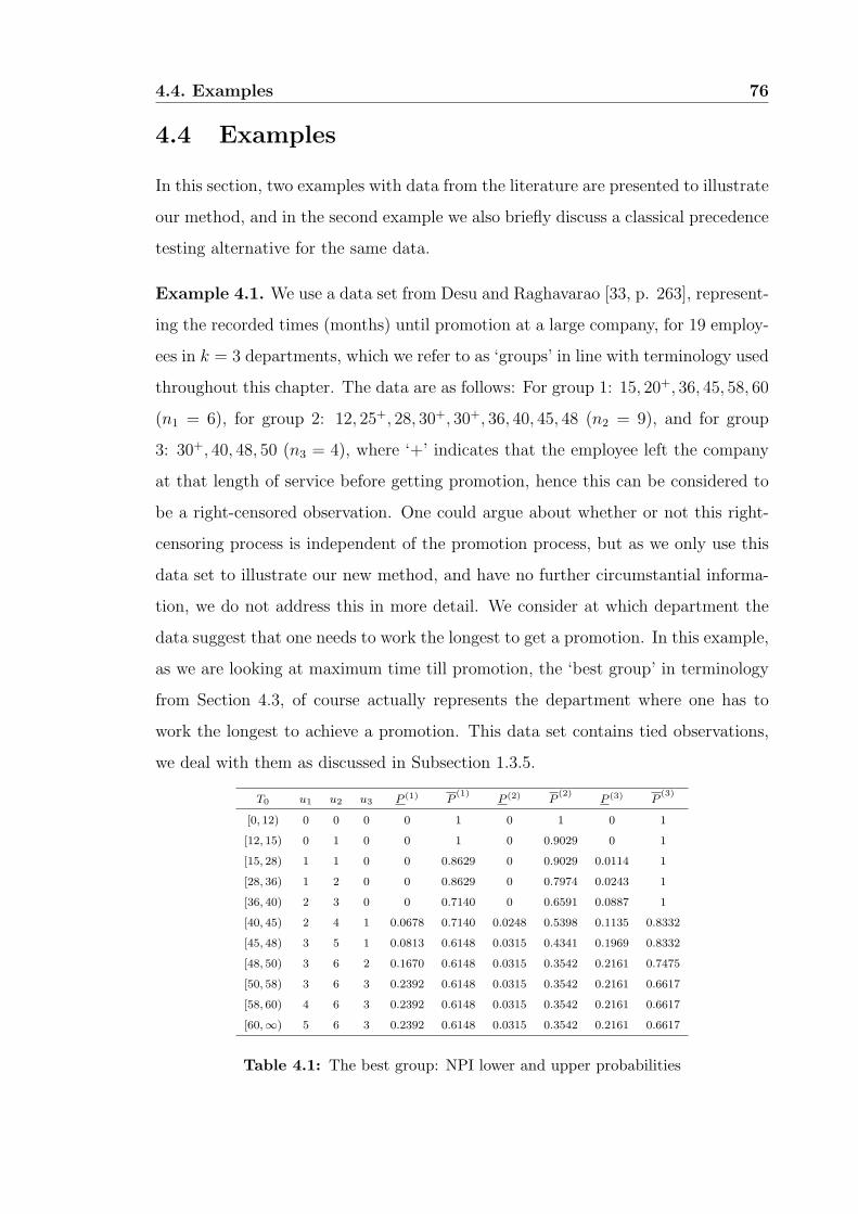
4.4. Examples 76
4.4 Examples
In this section, two examples with data from the literature are presented to illustrate
our method, and in the second example we also briefly discuss a classical precedence
testing alternative for the same data.
Example 4.1. We use a data set from Desu and Raghavarao [33, p. 263], represent-
ing the recorded times (months) until promotion at a large company, for 19 employ-
ees in k = 3 departments, which we refer to as ‘groups’ in line with terminology used
throughout this chapter. The data are as follows: For group 1: 15, 20+, 36, 45, 58, 60
(n1 = 6), for group 2: 12, 25+, 28, 30+, 30+, 36, 40, 45, 48 (n2 = 9), and for group
3: 30+, 40, 48, 50 (n3 = 4), where ‘+’ indicates that the employee left the company
at that length of service before getting promotion, hence this can be considered to
be a right-censored observation. One could argue about whether or not this right-
censoring process is independent of the promotion process, but as we only use this
data set to illustrate our new method, and have no further circumstantial informa-
tion, we do not address this in more detail. We consider at which department the
data suggest that one needs to work the longest to get a promotion. In this example,
as we are looking at maximum time till promotion, the ‘best group’ in terminology
from Section 4.3, of course actually represents the department where one has to
work the longest to achieve a promotion. This data set contains tied observations,
we deal with them as discussed in Subsection 1.3.5.
T0 u1 u2 u3 P (1) P(1)
P (2) P(2)
P (3) P(3)
[0, 12) 0 0 0 0 1 0 1 0 1
[12, 15) 0 1 0 0 1 0 0.9029 0 1
[15, 28) 1 1 0 0 0.8629 0 0.9029 0.0114 1
[28, 36) 1 2 0 0 0.8629 0 0.7974 0.0243 1
[36, 40) 2 3 0 0 0.7140 0 0.6591 0.0887 1
[40, 45) 2 4 1 0.0678 0.7140 0.0248 0.5398 0.1135 0.8332
[45, 48) 3 5 1 0.0813 0.6148 0.0315 0.4341 0.1969 0.8332
[48, 50) 3 6 2 0.1670 0.6148 0.0315 0.3542 0.2161 0.7475
[50, 58) 3 6 3 0.2392 0.6148 0.0315 0.3542 0.2161 0.6617
[58, 60) 4 6 3 0.2392 0.6148 0.0315 0.3542 0.2161 0.6617
[60,∞) 5 6 3 0.2392 0.6148 0.0315 0.3542 0.2161 0.6617
Table 4.1: The best group: NPI lower and upper probabilities
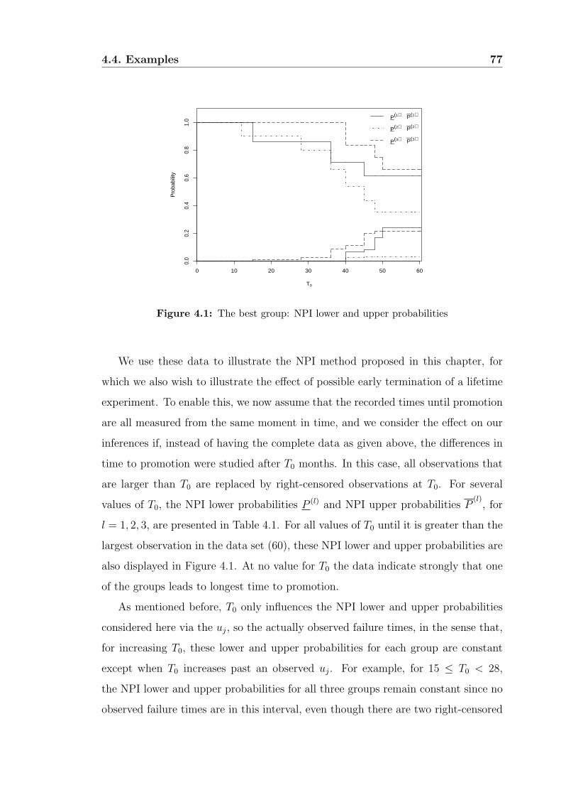
4.4. Examples 77
0 10 20 30 40 50 60
0.0
0.2
0.4
0.6
0.8
1.0
T0
Pro
babi
lity
P(1) P(1)
P(2) P(2)
P(3) P(3)
Figure 4.1: The best group: NPI lower and upper probabilities
We use these data to illustrate the NPI method proposed in this chapter, for
which we also wish to illustrate the effect of possible early termination of a lifetime
experiment. To enable this, we now assume that the recorded times until promotion
are all measured from the same moment in time, and we consider the effect on our
inferences if, instead of having the complete data as given above, the differences in
time to promotion were studied after T0 months. In this case, all observations that
are larger than T0 are replaced by right-censored observations at T0. For several
values of T0, the NPI lower probabilities P (l) and NPI upper probabilities P(l), for
l = 1, 2, 3, are presented in Table 4.1. For all values of T0 until it is greater than the
largest observation in the data set (60), these NPI lower and upper probabilities are
also displayed in Figure 4.1. At no value for T0 the data indicate strongly that one
of the groups leads to longest time to promotion.
As mentioned before, T0 only influences the NPI lower and upper probabilities
considered here via the uj, so the actually observed failure times, in the sense that,
for increasing T0, these lower and upper probabilities for each group are constant
except when T0 increases past an observed uj. For example, for 15 ≤ T0 < 28,
the NPI lower and upper probabilities for all three groups remain constant since no
observed failure times are in this interval, even though there are two right-censored
4.4. Examples 78
observations in this interval. These right-censored observations affect the NPI lower
and upper probabilities with larger values of T0, at later failure times, as the jump
sizes in these functions will increase. At T0 = 28, when the experiment would include
the failure time 28 for a unit of group 2, the upper probability for group 2 decreases
and the lower probability for group 3 increases. However, the lower probabilities for
groups 1 and 2 still remain 0 for T0 = 28, as there has not yet been an observed
failure for group 3 at that moment in time, so the data do not exclude the possibility
that units in group 3 would never fail. If the experiment is ended before the first
failure of a particular group occurs, as is the case for group 3 at T0 less than 40
in this example, then the extreme case corresponding to these lower probabilities
for groups 1 and 2, according to the NPI M -functions, allows the probability mass
related to failure for units of group 3 to go to infinity, which explains why the lower
probabilities for groups 1 and 2 remain equal to 0 until T0 increases past 40, the
smallest time at which a unit of group 3 fails.
If the experiment is stopped at T0 ∈ [15, 50), both the lower and upper proba-
bilities for group 3 are greater than the lower and upper probabilities, respectively,
for groups 1 and 2, as discussed before one could argue that this provides a weak
indication that group 3 leads to the longest times until promotion. However, the
large imprecision in these lower and upper probabilities indicates that the evidence
for such a claim is weak, so care must be taken when formulating any conclusion
along these lines. For larger values of T0, such that event times for most units have
been observed in the experiment, group 3 has most imprecision remaining, which
reflects that there are only few observations for group 3. 4
Example 4.2. In this example we use a data set considered by Lee and Desu
[49], which gives leukemia remission times (in days) for patients undergoing three
different treatments, so k = 3, and the numbers of patients per treatment are
n1 = 25, n2 = 19 and n3 = 22. The data are given in Table 4.2, where ‘+’
again denotes that an observation is right-censored. In this example, ‘better’ means
that a treatment leads to larger remission times. This data set was also used by
Chakraborti and van der Laan [16] to illustrate precedence testing, with Treatment
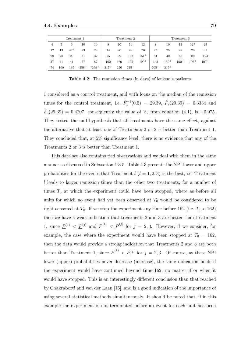
4.4. Examples 79
Treatment 1 Treatment 2 Treatment 3
4 5 9 10 10 8 10 10 12 8 10 11 12+ 23
12 13 20+ 23 28 14 20 48 70 25 25 28 28 31
28 28 29 31 32 75 99 103 161+ 31 40 48 89 124
37 41 41 57 62 162 169 195 199+ 143 159+ 190+ 196+ 197+
74 100 139 258+ 269+ 217+ 220 245+ 205+ 219+
Table 4.2: The remission times (in days) of leukemia patients
1 considered as a control treatment, and with focus on the median of the remission
times for the control treatment, i.e. F−11 (0.5) = 29.39, F2(29.39) = 0.3334 and
F3(29.39) = 0.4207, consequently the value of V , from equation (4.1), is −0.975.
They tested the null hypothesis that all treatments have the same effect, against
the alternative that at least one of Treatments 2 or 3 is better than Treatment 1.
They concluded that, at 5% significance level, there is no evidence that any of the
Treatments 2 or 3 is better than Treatment 1.
This data set also contains tied observations and we deal with them in the same
manner as discussed in Subsection 1.3.5. Table 4.3 presents the NPI lower and upper
probabilities for the events that Treatment l (l = 1, 2, 3) is the best, i.e. Treatment
l leads to larger remission times than the other two treatments, for a number of
times T0 at which the experiment could have been stopped, where as before all
units for which no event had yet been observed at T0 would be considered to be
right-censored at T0. If we stop the experiment any time before 162 (i.e. T0 < 162)
then we have a weak indication that treatments 2 and 3 are better than treatment
1, since P (1) < P (j) and P(1)
< P(j)
for j = 2, 3. However, if we consider, for
example, the case where the experiment would have been stopped at T0 = 162,
then the data would provide a strong indication that Treatments 2 and 3 are both
better than Treatment 1, since P(1)
< P (j) for j = 2, 3. Of course, as these NPI
lower (upper) probabilities never decrease (increase), the same indication holds if
the experiment would have continued beyond time 162, no matter if or when it
would have stopped. This is an interestingly different conclusion than that reached
by Chakraborti and van der Laan [16], and is a good indication of the importance of
using several statistical methods simultaneously. It should be noted that, if in this
example the experiment is not terminated before an event for each unit has been
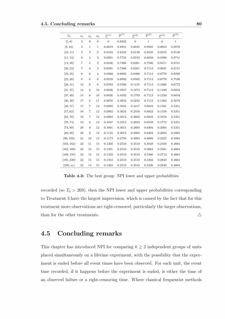
4.5. Concluding remarks 80
T0 u1 u2 u3 P (1) P(1)
P (2) P(2)
P (3) P(3)
[5, 8) 2 0 0 0 0.9232 0 1 0 1
[8, 10) 3 1 1 0.0019 0.8851 0.0045 0.9505 0.0053 0.9570
[10, 11) 5 3 2 0.0103 0.8102 0.0139 0.8535 0.0253 0.9156
[11, 13) 6 4 3 0.0201 0.7734 0.0243 0.8059 0.0396 0.8741
[13, 20) 7 5 3 0.0246 0.7366 0.0281 0.7586 0.0571 0.8741
[20, 23) 7 6 3 0.0291 0.7366 0.0281 0.7113 0.0681 0.8741
[23, 25) 8 6 4 0.0380 0.6992 0.0408 0.7113 0.0776 0.8339
[25, 28) 8 6 6 0.0559 0.6992 0.0592 0.7113 0.0776 0.7536
[28, 31) 12 6 8 0.0703 0.5598 0.1155 0.7113 0.1066 0.6772
[31, 37) 14 6 10 0.0826 0.4927 0.1674 0.7113 0.1189 0.6034
[37, 40) 15 6 10 0.0826 0.4592 0.1793 0.7113 0.1250 0.6034
[40, 48) 17 6 11 0.0876 0.3934 0.2232 0.7113 0.1362 0.5678
[48, 57) 17 7 12 0.0992 0.3934 0.2417 0.6823 0.1501 0.5351
[57, 62) 18 7 12 0.0992 0.3624 0.2550 0.6823 0.1559 0.5351
[62, 70) 19 7 12 0.0992 0.3313 0.2682 0.6823 0.1618 0.5351
[70, 74) 19 8 12 0.1047 0.3313 0.2682 0.6558 0.1773 0.5351
[74, 89) 20 9 12 0.1091 0.3015 0.2803 0.6304 0.2004 0.5351
[89, 99) 20 9 13 0.1125 0.3015 0.2985 0.6304 0.2004 0.5085
[99, 103) 21 10 13 0.1173 0.2750 0.3093 0.6069 0.2225 0.5085
[103, 162) 22 11 15 0.1260 0.2510 0.3510 0.5848 0.2450 0.4664
[162, 169) 22 12 15 0.1291 0.2510 0.3510 0.5664 0.2581 0.4664
[169, 195) 22 13 15 0.1322 0.2510 0.3510 0.5480 0.2713 0.4664
[195, 220) 22 15 15 0.1353 0.2510 0.3510 0.5302 0.2840 0.4664
[220,∞) 22 14 15 0.1404 0.2510 0.3510 0.5226 0.2840 0.4664
Table 4.3: The best group: NPI lower and upper probabilities
recorded (so T0 > 269), then the NPI lower and upper probabilities corresponding
to Treatment 3 have the largest imprecision, which is caused by the fact that for this
treatment more observations are right-censored, particularly the larger observations,
than for the other treatments. 4
4.5 Concluding remarks
This chapter has introduced NPI for comparing k ≥ 2 independent groups of units
placed simultaneously on a lifetime experiment, with the possibility that the exper-
iment is ended before all event times have been observed. For each unit, the event
time recorded, if it happens before the experiment is ended, is either the time of
an observed failure or a right-censoring time. Where classical frequentist methods
4.5. Concluding remarks 81
in statistics tend to base such comparison on hypotheses tests, the NPI approach
directly compares random failure times of further units from these groups, which are
assumed to be related to the observations per group through the assumption A(n).
We consider it an advantage that, as clearly shown in Examples 4.1 and 4.2 for
smaller values of T0, corresponding NPI lower and upper probabilities may differ so
much that they do not point towards clear decisions. This makes clear that, in order
to derive stronger guidance, more information is needed, which in this application
area would imply to either continue the experiment or to repeat it with more units
involved. Of course, if there are no possibilities to gain further information, the
wide bounds do not lead to indecision, but they just make clear that the data
and method used do not strongly indicate a preference for any of the groups. In
this case, the data and NPI method may still provide some weak indications to
support a specific choice, whereas alternative statistical methods, if they lead to a
null hypothesis of ‘equal probability distributions’ not being rejected, would provide
very little guidance on what group to choose if one must do so.
We only considered comparison of different groups by focusing on a single group
being best, defined in terms of maximum value of the random lifetime for a future
observation. Generalization to consider subsets of groups, either such that they
contain the best one or that all selected groups are better than all not-selected
groups, is achievable along the lines of Chapter 3 and Coolen and van der Laan [25].
Chapter 5
Progressive Censoring
5.1 Introduction
One topic that has led to a substantial literature in frequentist statistics involving
right-censored data is progressive censoring [3, 47], where, during a lifetime experi-
ment, non-failing units are withdrawn from the experiments. This could be done to
save cost or time, but it may also be useful, at the moment a unit fails, to study the
unit in detail in comparison with units in the same experiment that have not failed,
to get better knowledge about the underlying cause of failure [61, 67]. There may
also be specific circumstances which cause some units to fail due to reasons unre-
lated to the experimentation [18], and it may occur that an individual or unit drops
out of the study before the end of the experiment [3], which also makes progressive
censoring schemes useful. Several progressive censoring schemes have been consid-
ered in the literature, including progressive Type-I censoring, progressive Type-II
censoring [3] and Type-II progressively hybrid censoring [46].
In this chapter we present Nonparametric Predictive Inference (NPI) for com-
parison of two groups under different progressive censoring schemes. Section 5.2
provides a short overview of progressive censoring schemes for as far as required in
this chapter. In Sections 5.3, 5.4 and 5.5 we present the main results of this chapter,
namely the NPI lower and upper probabilities for the event that the lifetime of a
future unit from group Y is greater than the lifetime of a future unit from group
X, under the three different progressive censoring schemes discussed in Section 5.2.
82
5.2. Progressive censoring schemes 83
The main focus is on the progressive Type-II censoring scheme, as it has received
most attention in the literature, for which the results stated are proved in detail.
However, we also briefly present NPI for the two other schemes, the proofs of these
follow the same lines of reasoning as for the progressive Type-II censoring results
and are not included in full detail. NPI for these scenarios, and for a few related
situations, is illustrated and discussed via an example, and the chapter ends with
some concluding remarks in Section 5.7.
5.2 Progressive censoring schemes
This section provides a brief overview of three progressive censoring schemes, called
progressive Type-I censoring, progressive Type-II censoring and Type-II progres-
sively hybrid censoring. In a progressive Type-I censoring scheme, see Figure 5.1(a),
n units are placed on a lifetime experiment. Of these n units, r fail during the
experiment, we assume ( in order to simplify presentation of the approach presented
in this chapter) that they fail at r different failure times x1 < x2 < . . . < xr. At
m times T1 < T2 < . . . < Tm, some further units may be randomly withdrawn
from the experiment, leading to right-censored observations for their corresponding
lifetimes. At such a time Tj (j = 1, . . . ,m) where progressive censoring is taking
place, let Rj denote the number of units that are removed from the experiment
without having failed. We assume that the experiment finishes at time Tm, hence
Tm > xr and Rm = n − r −∑m−1j=1 Rj. For use later in this chapter, we define sj
to be the number of failures between the consecutive right-censoring times Tj−1 and
Tj, so sj = #Tj−1 < xi ≤ Tj : i = 1, . . . , r (j = 2, . . . ,m), and s1 is the num-
ber of failures before T1. Then the data from this experiment, under a progressive
Type-I censoring scheme, consist of r =∑m
j=1 sj observed failure times and n − r
right-censoring times.
In a progressive Type-II censoring scheme, see Figure 5.1(b), the number of units
to be observed to fail is fixed, let this number be r. At each observed failure time,
which we again assume to be r different times x1 < x2 < . . . < xr, some further
units which have not failed are randomly removed from the experiment, and at the

5.2. Progressive censoring schemes 84
R1 R2 Rm
r r r×× × × × × × ×0 T1 T2 . . . Tm ∞
(a) Progressive Type-I censoring
R1 R2 Rr
r r r
0 x1 x2 . . . xr ∞(b) Progressive Type-II censoring
R1 R2 RJ RT
r r r r
0 x1 x2 . . . xJ T ∞(c) Type-II progressively hybrid censoring
Figure 5.1: Three different progressive censoring schemes
last failure time xr all the remaining units are removed from the experiment. Let Ri
denote the number of units that have not failed but are removed from the experiment
at failure time xi, for i = 1, . . . , r, then Rr = n− r −∑r−1i=1 Ri. The data consist of
the r observed failure times x1 < x2 < . . . < xr, together with the numbers of units
with right-censored lifetimes at each of these failure times, which information we
denote by R = (R1, R2, . . . , Rr). Some special cases of this censoring scheme occur
if r = n, then Ri = 0 for all i = 1, . . . , r, which means that there is no censoring
actually occurring, and if we have Ri = 0 for all i = 1, . . . , r−1 and Rr = n−r then
we obtain a conventional Type-II censored sample with censoring only due to the
experiment being stopped before all units have failed. A special case of progressive
Type-II censoring is the ‘throw away scheme’, presented by Cohen and Clifford [17],
in which a fixed number of units is withdrawn from the experiment at each observed
breakdown time. Such special cases are not highlighted further in this chapter, but
are briefly considered in Example 5.1.
In a progressive Type-II censored experiment, it might take a very long time
5.2. Progressive censoring schemes 85
to reach the prefixed number r. Therefore, it may be attractive to consider an ex-
periment which is ended as soon as either r failures have been observed, or at a
specific time, say T , whichever occurs first. In the latter case, the lifetimes of all the
remaining units in the experiment at time T are right-censored at this time, in addi-
tion to the right-censored lifetimes of units that were progressively censored during
the experiment at different failure times before T . This scenario is called Type-II
progressive hybrid censoring, and is a mixture of progressive Type-II censoring and
conventional Type-I censoring, see Figure 5.1(c). Let xJ denote the largest observed
failure time prior to T , and again we assume that no failures coincide, so the ob-
served failure times are x1 < x2 < . . . < xJ < T . At xi, for i = 1, . . . , J , Ri units
are randomly withdrawn from the experiment. Finally, all the remaining RT units
are withdrawn from the experiment at time T , so RT = n− J −∑Ji=1 Ri.
As mentioned above, one may be interested in comparing two independent pop-
ulations or treatments, say X and Y . For example, X may refer to a control group
and Y to a new treatment group [7], where statistical inference would be aimed
at investigating whether or not Y can be considered to provide an improvement
compared to X. Most classical statistics methods presented in the literature [7],
including several nonparametric methods, approach such comparison problems by
hypothesis testing. In particular, they tend to assume continuous cumulative dis-
tribution functions for the random quantities of interest, say F (·) corresponding to
X and G(·) corresponding to Y , and test the null hypothesis that the two groups
X and Y are the same with regard to the random quantity of interest, so they test
H0 : F (x) = G(x), for all x, against the hypothesis that group Y tends to have
greater lifetimes than group X, expressed via the stochastic dominance hypothesis
H1 : F (x) ≥ G(x) with strict inequality holding for at least one x. The approach
presented in this chapter is fundamentally different, with comparisons formulated
directly in terms of a future observation for each of the two groups considered, a
method which does not involve testing of hypotheses.
We focus on the progressive Type-II censoring scheme, for which in the literature
two cases are considered, depending on whether progressive censoring has been ap-
plied to only one group or to both groups. In the first case, the progressive Type-II
5.2. Progressive censoring schemes 86
censoring scheme applies to only one group, say group Y , and it is assumed that the
data from group X result from an experiment without progressive censoring, but
which is also ended when the experiment of group Y ends, at failure time yr from
group Y , so the group X data consist of failure times prior to yr and right-censored
lifetimes at yr, resulting from standard Type-II censoring at yr. For this case, Ng and
Balakrishnan [5, 67] have proposed several tests, including the weighted precedence
test, the weighted maximal precedence test and the maximal Wilcoxon rank-sum
precedence test as extensions of classical precedence tests that are suitable for this
scenario. Bairamov and Eryilmaz [2] considered exceedance statistics for the same
setting.
As the second case, one considers the situation with progressive Type-II censoring
applied independently to both groups X and Y . Recently, Balakrishnan et al. [7]
introduced a precedence test based on placement statistics with progressive censoring
for both groups. The proposed precedence test statistic, P(s), is basically the number
of failures from group X that precede the sth (1 ≤ s ≤ ry) failure from group Y ,
where ry is the number of failures from group Y . Two further precedence tests are
proposed by Balakrishnan et al. [8, 9] for progressive censoring in both samples. The
first is a Wilcoxon type rank-sum precedence test, T(ry), where all censored items
are assumed to fail immediately after the censoring occurs. Then T(ry) is defined as
the sum of the ranks of the X observations in the combined sample (i.e. X and Y
combined together) [8, 9]. The second test statistic, Q(ry), is based on the Kaplan-
Meier estimator [44] of the cumulative distribution functions F and G. Let Qj be
the number of failures from group X between the (j − 1)th and jth failure from
group Y for which F (xi) ≥ G(yj), for j = 1, 2, . . . , ry where y0 = 0. Then,
Q(ry) =
ry∑
j=1
Qj +1
2Qry+1
where the Qry+1 is obtained by assuming that the remaining unobserved failures
from group X (i.e. the failures from group X that greater than yry) occur before
the censored items from group Y at yry for which F (xi) ≥ G(yry+1), where yry+1 is
taken as the (ry +1)th progressive Type-II censored order statistic with progressive
censoring scheme (Ry1, . . . , R
yry−1, 0, ny−ry−1−∑ry−1
j=1 Ryj ). For the null distributions
5.3. NPI for progressive Type-II censoring 87
of these test statistics and for more details we refer to [8, 9]. The NPI approach is
compared to these methods in Example 5.1.
5.3 NPI for progressive Type-II censoring
For the progressive Type-II censoring scheme, n units are placed on a lifetime ex-
periment, and for r of these units actual failure times are observed during the ex-
periment, while at each observed failure time for one of these r units, some of the
remaining units may be withdrawn from the experiment, until the r-th failure time
when the experiment is ended, and hence all remaining units are removed from the
experiment. We can consider the n − r progressively censored units (according to
the scheme R = (R1, R2, . . . , Rr)) as being grouped in blocks, each consisting of
units censored at a specific observed failure time. Hence, this leads to all censored
units in one block to be censored at the same time, which is dealt with by rc-A(n) as
described below. For ease of notation, we assume throughout that there are no ties
between the observed failure times, the tied right-censoring times do not provide
complications and actually simplify the approach as discussed below. In addition,
we use x0 = 0 and xr+1 = ∞. The following theorem provides the M -functions re-
quired for NPI applied to comparison of lifetime data under the progressive Type-II
censoring scheme, together with the total probability mass assigned to the interval
(xi, xi+1).
Theorem 5.1. To apply NPI to data from an experiment with a progressive Type-
II censoring scheme with R = (R1, R2, . . . , Rr), the assumption rc-A(n) implies that
the probability distribution for a nonnegative random quantity Xn+1 on the basis
of data including r real and (n− r) progressively censored observations, is partially
specified by the following M -function values, for i = 0, 1, . . . , r,
MX(xi, xi+1) = MXn+1(xi, xi+1) =1
n+ 1
i−1∏
k=1
n− k −∑k−1l=1 Rl + 1
n− k −∑kl=1Rl + 1
(5.1)
MX(x+i , xi+1)=MXn+1(x
+i , xi+1)=
[
Ri
n− i−∑il=1Rl+1
]
MX(xi, xi+1) (5.2)
5.3. NPI for progressive Type-II censoring 88
where x+i is used to indicate a value infinitessimally greater than xi, which can
be interpreted as representing the lower bound for the interval that would contain
the actual lifetimes for all units censored at xi. Then the total probability mass
assigned to the interval (xi, xi+1) is the sum of the two M -functions corresponding
to (xi, xi+1) and (x+i , xi+1) (for i = 0, 1, . . . , r), and is given by
PX(xi, xi+1) = P (Xn+1 ∈ (xi, xi+1)) =1
n+ 1
i∏
k=1
n− k −∑k−1l=1 Rl + 1
n− k −∑kl=1Rl + 1
(5.3)
Proof. We can write the observations, both failure times and right-censoring times,
of n units from group X as given below, in which we assume that all observations are
different values for ease of presentation, but for tied right-censored observations one
can derive the exact NPI results as limiting situation with the difference between
such right-censoring times becoming infinitesimally small. We follow Coolen and
Yan [27] in assuming, which is also standard in the wider literature, that coinciding
failure and right-censoring times are actually such that the latter is slightly larger
than the failure time. Let the data be
0 < x1 < c11 < . . . < c1R1< x2 < c21 < . . . < c2R2
< x3 < . . .
< . . . < xi < ci1 < . . . < ciRi< xi+1 < . . . < xr < cr1 < . . . < crRr
< ∞
For the setting considered in this chapter, cili is actually the right-censoring time of
the lith unit censored at xi, for i = 1, . . . , r and li = 1, . . . , Ri.
For any block k (k = 1, . . . , r), xk < ck1 < . . . < cklk < . . . < ckRk< xk+1, nck
lk
is
the number of units at risk at cklk , that is ncklk
= n− k − (lk − 1)−∑k−1l=1 Rl. Then,
and from (1.3),
MX(xi, xi+1) =1
n+ 1
∏
k:ck<xi
nck + 1
nck
=1
n+ 1
i−1∏
k=1
Rk∏
lk=1
ncklk
+ 1
ncklk
=1
n+ 1
i−1∏
k=1
n− k −∑k−1l=1 Rl + 1
n− k −∑kl=1Rl + 1
similar, and from (1.6),
PX(xi, xi+1) =1
n+ 1
∏
k:ck<xi+1
nck + 1
nck
=1
n+ 1
i∏
k=1
n− k −∑k−1l=1 Rl + 1
n− k −∑kl=1Rl + 1
5.3. NPI for progressive Type-II censoring 89
since MX(x+i , xi+1) = PX(xi, xi+1)−MX(xi, xi+1), then
MX(x+i , xi+1) =
1
n+ 1
[
i−1∏
k=1
n− k −∑k−1l=1 Rl + 1
n− k −∑kl=1 Rl + 1
][
Ri
n− i−∑il=1Rl + 1
]
In this section we present NPI to compare two groups, say X and Y , when one
(or both) is (are) progressively censored. Throughout, we consider the two groups
to be completely independent. In NPI, the comparison of groups X and Y is in
terms of lower and upper probabilities for the event that a single future observation
from group Y is greater than a single future observation from group X, where lower
and upper probabilities are used in order to keep inferential assumptions, added to
the data observed, restricted.
Suppose that we have two independent groups, X and Y , consisting of nx
and ny units, all placed on a lifetime experiment. Units of both groups are pro-
gressively Type-II censored with the schemes Rx = (Rx1 , R
x2 , . . . , R
xrx) and Ry =
(Ry1, R
y2, . . . , R
yry). In practice, for example, group X could be a control group, with
a new treatment applied to units in group Y , and the aim might be to draw con-
clusions on whether or not the new treatment group tends to provide improved
lifetimes. Given the data, Rx, Ry, and with the appropriate assumptions rc-A(nx)
and rc-A(ny) for the respective groups, Theorem 5.2 presents the NPI lower and up-
per probabilities for the event that the next future observation from group Y , Yny+1,
is greater than the next future observation from group X, Xnx+1.
Theorem 5.2. The NPI lower and upper probabilities for the event that the next
future observation from group Y is greater than the next future observation from
group X, under the progressive Type-II censoring scheme for both groups, are
P(
Yny+1 > Xnx+1
)
=
ry∑
j=0
rx∑
i=0
1xi+1 < yjPX(xi, xi+1)
P Y (yj, yj+1) (5.4)
P(
Yny+1 > Xnx+1
)
=
ry∑
j=0
rx∑
i=0
1xi < yj+1PX(xi, xi+1)
P Y (yj, yj+1) (5.5)
with PX and P Y according to equation (5.3).
5.3. NPI for progressive Type-II censoring 90
Proof. The NPI lower probability for the event Xnx+1 < Yny+1, given the data and
progressive Type-II censoring schemes Rx and Ry, is derived as follows:
P = P (Xnx+1 < Yny+1) =ry∑
j=0
P (Xnx+1 < Yny+1, Yny+1 ∈ (yj, yj+1))
≥ry∑
j=0
P (Xnx+1 < yj)MY (yj, yj+1) + P (Xnx+1 < y+j )M
Y (y+j , yj+1)
=ry∑
j=0
P (Xnx+1 < yj)
MY (yj, yj+1) +MY (y+j , yj+1)
=ry∑
j=0
P (Xnx+1 < yj)PY (yj, yj+1)
≥ry∑
j=0
rx∑
i=0
1xi+1 < yjPX(xi, xi+1)PY (yj, yj+1)
The first inequality follows by putting all probability masses for Yny+1 corresponding
to the intervals (yj, yj+1) and (y+j , yj+1) (j = 1, . . . , ry) to the left end points of these
intervals, and by using Lemma 1.4 for the nested intervals (yj, yj+1) and (y+j , yj+1).
The second inequality follows by putting all probability masses for Xnx+1 corre-
sponding to the intervals (xi, xi+1) and (x+i , xi+1) (i = 1, . . . , rx) to the right end
points of these intervals. We should notice that P (Xnx+1 < y+j ) = P (Xnx+1 < yj)
since the Ryj units that are right-censored at yj do not cause these probabilities to
be different due to the assumption of an infinitesimal difference between y+j and yj,
and due to the fact that the M -functions in NPI are generally assigned to open
intervals between observations.
The NPI upper probability is obtained in a similar way, but now all probability
masses for the random quantities involved are put at the opposite end points of
the respective intervals. We should notice that 1x+i < yj+1 = 1xi < yj+1 by
arguments similar to those used in the derivation above for the lower probability.
P = P (Xnx+1 < Yny+1) =ry∑
j=0
P (Xnx+1 < Yny+1, Yny+1 ∈ (yj, yj+1))
≤ry∑
j=0
P (Xnx+1 < yj+1)PY (yj, yj+1)
≤ry∑
j=0
P Y (yj, yj+1)rx∑
i=0
1xi<yj+1MX(xi, xi+1)+1x+i<yj+1MX(x+
i , xi+1)
=ry∑
j=0
rx∑
i=0
P Y (yj, yj+1)1xi < yj+1
MX(xi, xi+1) +MX(x+i , xi+1)
=ry∑
j=0
rx∑
i=0
1xi < yj+1PX(xi, xi+1)PY (yj, yj+1)
5.4. NPI for progressive Type-I censoring 91
The use of these NPI lower and upper probabilities is illustrated in Example 5.1.
Next we present the NPI lower and upper probabilities for the two other progressive
censoring schemes discussed in Section 5.2, for these all ingredients required for the
complete derivations are provided, but detailed proofs are not presented as these
follow the general lines of the proof above.
5.4 NPI for progressive Type-I censoring
In a progressive Type-I censoring scheme for n units on a lifetime experiment, as
discussed in Section 5.2, Rj units are withdrawn from the experiment at Tj (j =
1, . . . ,m), and for a total of r =∑m
j=1 sj units the actual failure times will be
observed, where sj is the number of observed failure times between Tj−1 and Tj.
Again assuming no ties among the observed failure times, the data can be written
as
· · · < Tj−1 < xj1 < · · · < xj
sj< Tj < xj+1
1 < . . . < xj+1sj+1 < Tj+1 < . . .
Rj−1 Rj Rj+1
where xjij
is the ijth observed failure time between Tj−1 and Tj (ij = 1, . . . , sj,
j = 1, . . . ,m). For this situation, the NPI approach for comparison of two groups,
X and Y , similarly as presented in the previous section, is as follows. Let
Bj =1
n+ 1
j∏
k=1
n−∑kl=1 sl −
∑k−1l=1 Rl + 1
n−∑kl=1 sl −
∑kl=1Rl + 1
then the M -functions corresponding to a progressive Type-I censoring scheme, are
(for j = 1, . . . ,m and ij = 1, . . . , sj)
MX(0, x11) = B1 , MX(xj
ij, xj
ij+1) = Bj−1 ,
MX(Tj, xj+11 ) =
[
Rj
n−∑jl=1 sl −
∑jl=1Rl+1
]
Bj−1 , PX(xjij, xj
ij+1) = Bj
where xj+11 ( xj
sj) is the first (last) failure time observed after (before) we removed
Rj units at time Tj, and where xjsj+1 = xj+1
1 and xm+11 = ∞.
Now we consider two groups X and Y under such a progressive Type-I censoring
scheme, with right-censoring times T xa (a = 1, . . . , p) and T y
b (b = 1, . . . , q), such that
5.5. NPI for Type-II progressively hybrid censoring 92
Rxa (Ry
b ) units of group X (Y ) that have not failed are withdrawn from the experi-
ment at T xa (T y
b ). Then the numbers of failures from both groups are rx =∑p
a=1 sxa
and ry =∑q
b=1 syb , where sxa (syb) is the number of failures between the consecutive
right-censoring times T xa−1 and T x
a (T yb−1 and T y
b ). The NPI lower probability for the
event Xnx+1 < Yny+1 in this situation is
P =
q∑
b=1
syb∑
ib=1
P (Xnx+1 < ybib)MY (ybib , y
bib+1) + P (Xnx+1 < T y
b )MY (T y
b , yb+11 )
where
P (Xnx+1 < ·) =p∑
a=1
sxa∑
ia=0
1xaia+1 < ·PX(xa
ia , xaia+1)
and the corresponding NPI upper probability is
P =
q∑
b=1
syb∑
ib=0
P (Xnx+1 < ybib+1)PY (ybib , y
bib+1)
where
P (Xnx+1 < ·) =p∑
a=1
sxa∑
ia=0
1xaia < ·MX(xa
ia , xaia+1) + 1T x
a < ·MX(T xa , x
a+11
As mentioned before, detailed justification of these results follows the same lines as
the proof in the previous section. The special case where such progressive censoring
is only applied to one of the two groups also follows straightforwardly, and will be
briefly illustrated in Example 5.1.
5.5 NPI for Type-II progressively hybrid censor-
ing
Under this scheme of progressive censoring, that was also introduced in Section 5.2,
one only observes the J failure times which occur prior to time T , and at failure
time xi (i = 1, . . . , J) Ri units that have not failed are removed, and finally the
experiment is ended at time T , when the RT remaining units are removed from
the experiment. For this progressive censoring scheme, we can use the same M -
functions as given in (5.1) and (5.2) for the intervals (xi, xi+1) and (x+i , xi+1), where
5.5. NPI for Type-II progressively hybrid censoring 93
i = 0, 1, . . . , J , x0 = 0 and xJ+1 = ∞. However, for the additional interval (T,∞),
the M -function value is
MX(T,∞) =1
n+ 1
[
RT
n− J −∑Ji=1 Ri −RT + 1
]
J∏
k=1
n− k −∑k−1l=1 Rl + 1
n− k −∑kl=1 Rl + 1
This also leads to the same formula (5.3) being appropriate for the probability
PX(xi, xi+1), for i = 0, 1, . . . , J −1, while for the last interval we have PX(xJ ,∞) =
MX(xJ ,∞) +MX(x+J ,∞) +MX(T,∞).
NPI for comparison of two groups, X and Y , under such Type-II progressively hy-
brid censoring with (Rx1 , R
x2 , . . . , R
xJx, Rx
Tx) and (Ry1, R
y2, . . . , R
yJy, Ry
T y), respectively,
is again based on the NPI lower and upper probabilities for the direct comparison
of one future observation from each group, so for the event Xnx+1 < Yny+1. For this
censoring scheme, these NPI lower and upper probabilities are
P =
Jy∑
j=0
P (Xnx+1 < yj)PY (yj, yj+1)+P (Xnx+1 < T y)−P (Xnx+1 < yJy)MY (T y,∞)
where
P (Xnx+1 < ·) =Jx∑
i=0
1xi+1 < ·PX(xi, xi+1)
and
P =
Jy∑
j=0
P (Xnx+1 < yj+1)PY (yj, yj+1) + P (Xnx+1 < ∞)MY (T y,∞)
where
P (Xnx+1 < ·) =Jx∑
i=0
1xi < ·PX(xi, xi+1+ 1T x < · − 1xJx < ·MX(T x,∞)
Detailed justification of these results is again similar to the proof given for the
progressive Type-II censoring scheme, and this case is also illustrated in Example
5.1.
Finally, let us briefly comment on what could be considered a special case of the
progressive censoring schemes described above, namely if we just decide to terminate
the lifetime experiment at a certain time point, say T0, which could be a specific
failure time, and with no other censoring applied. In this case, we have Rx =
(0, 0, . . . , Rxrx) and Ry = (0, 0, . . . , Ry
ry), where Rxrx = nx−rx and Ry
ry = ny−ry. NPI
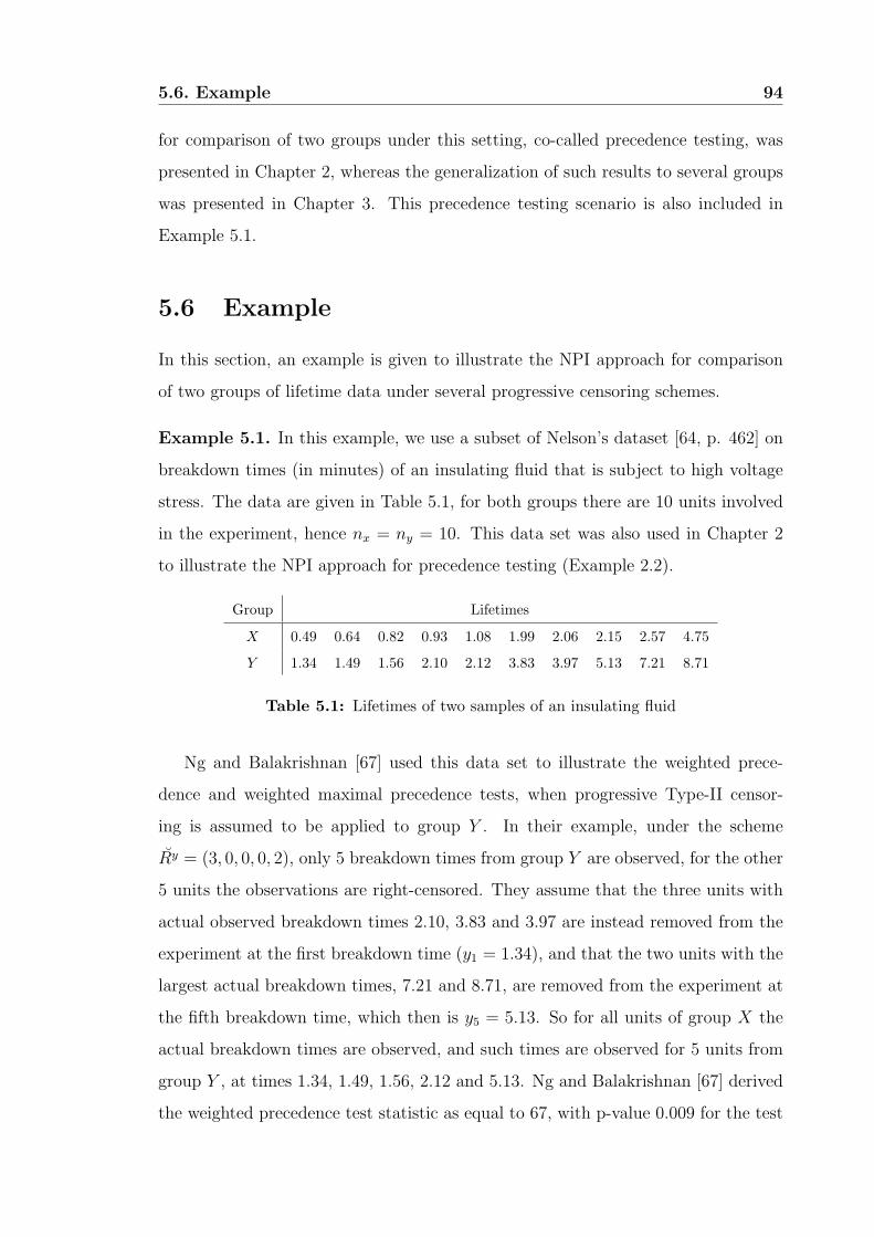
5.6. Example 94
for comparison of two groups under this setting, co-called precedence testing, was
presented in Chapter 2, whereas the generalization of such results to several groups
was presented in Chapter 3. This precedence testing scenario is also included in
Example 5.1.
5.6 Example
In this section, an example is given to illustrate the NPI approach for comparison
of two groups of lifetime data under several progressive censoring schemes.
Example 5.1. In this example, we use a subset of Nelson’s dataset [64, p. 462] on
breakdown times (in minutes) of an insulating fluid that is subject to high voltage
stress. The data are given in Table 5.1, for both groups there are 10 units involved
in the experiment, hence nx = ny = 10. This data set was also used in Chapter 2
to illustrate the NPI approach for precedence testing (Example 2.2).
Group Lifetimes
X 0.49 0.64 0.82 0.93 1.08 1.99 2.06 2.15 2.57 4.75
Y 1.34 1.49 1.56 2.10 2.12 3.83 3.97 5.13 7.21 8.71
Table 5.1: Lifetimes of two samples of an insulating fluid
Ng and Balakrishnan [67] used this data set to illustrate the weighted prece-
dence and weighted maximal precedence tests, when progressive Type-II censor-
ing is assumed to be applied to group Y . In their example, under the scheme
Ry = (3, 0, 0, 0, 2), only 5 breakdown times from group Y are observed, for the other
5 units the observations are right-censored. They assume that the three units with
actual observed breakdown times 2.10, 3.83 and 3.97 are instead removed from the
experiment at the first breakdown time (y1 = 1.34), and that the two units with the
largest actual breakdown times, 7.21 and 8.71, are removed from the experiment at
the fifth breakdown time, which then is y5 = 5.13. So for all units of group X the
actual breakdown times are observed, and such times are observed for 5 units from
group Y , at times 1.34, 1.49, 1.56, 2.12 and 5.13. Ng and Balakrishnan [67] derived
the weighted precedence test statistic as equal to 67, with p-value 0.009 for the test
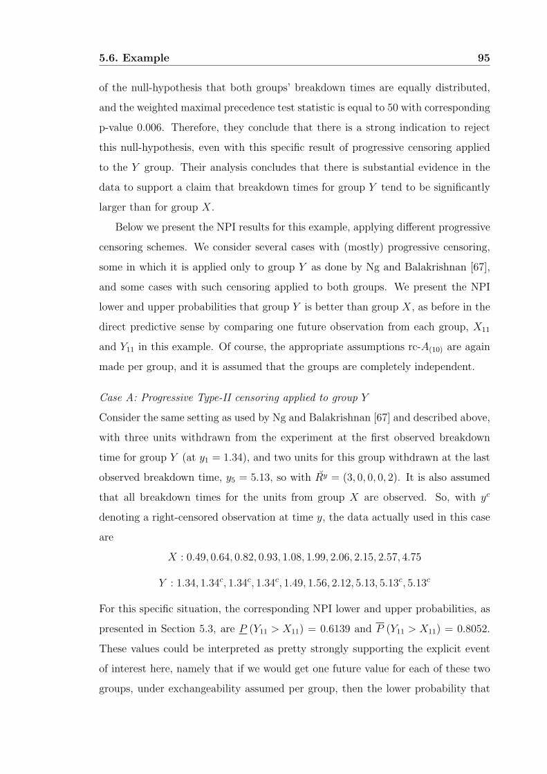
5.6. Example 95
of the null-hypothesis that both groups’ breakdown times are equally distributed,
and the weighted maximal precedence test statistic is equal to 50 with corresponding
p-value 0.006. Therefore, they conclude that there is a strong indication to reject
this null-hypothesis, even with this specific result of progressive censoring applied
to the Y group. Their analysis concludes that there is substantial evidence in the
data to support a claim that breakdown times for group Y tend to be significantly
larger than for group X.
Below we present the NPI results for this example, applying different progressive
censoring schemes. We consider several cases with (mostly) progressive censoring,
some in which it is applied only to group Y as done by Ng and Balakrishnan [67],
and some cases with such censoring applied to both groups. We present the NPI
lower and upper probabilities that group Y is better than group X, as before in the
direct predictive sense by comparing one future observation from each group, X11
and Y11 in this example. Of course, the appropriate assumptions rc-A(10) are again
made per group, and it is assumed that the groups are completely independent.
Case A: Progressive Type-II censoring applied to group Y
Consider the same setting as used by Ng and Balakrishnan [67] and described above,
with three units withdrawn from the experiment at the first observed breakdown
time for group Y (at y1 = 1.34), and two units for this group withdrawn at the last
observed breakdown time, y5 = 5.13, so with Ry = (3, 0, 0, 0, 2). It is also assumed
that all breakdown times for the units from group X are observed. So, with yc
denoting a right-censored observation at time y, the data actually used in this case
are
X : 0.49, 0.64, 0.82, 0.93, 1.08, 1.99, 2.06, 2.15, 2.57, 4.75
Y : 1.34, 1.34c, 1.34c, 1.34c, 1.49, 1.56, 2.12, 5.13, 5.13c, 5.13c
For this specific situation, the corresponding NPI lower and upper probabilities, as
presented in Section 5.3, are P (Y11 > X11) = 0.6139 and P (Y11 > X11) = 0.8052.
These values could be interpreted as pretty strongly supporting the explicit event
of interest here, namely that if we would get one future value for each of these two
groups, under exchangeability assumed per group, then the lower probability that
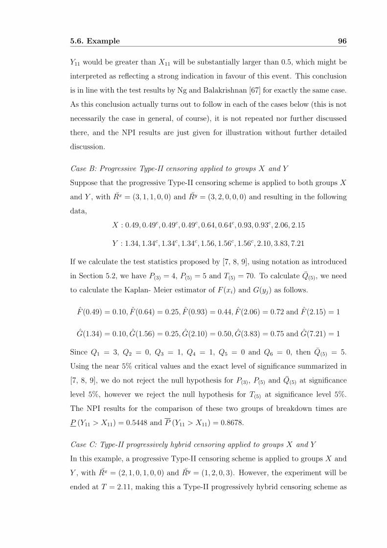
5.6. Example 96
Y11 would be greater than X11 will be substantially larger than 0.5, which might be
interpreted as reflecting a strong indication in favour of this event. This conclusion
is in line with the test results by Ng and Balakrishnan [67] for exactly the same case.
As this conclusion actually turns out to follow in each of the cases below (this is not
necessarily the case in general, of course), it is not repeated nor further discussed
there, and the NPI results are just given for illustration without further detailed
discussion.
Case B: Progressive Type-II censoring applied to groups X and Y
Suppose that the progressive Type-II censoring scheme is applied to both groups X
and Y , with Rx = (3, 1, 1, 0, 0) and Ry = (3, 2, 0, 0, 0) and resulting in the following
data,
X : 0.49, 0.49c, 0.49c, 0.49c, 0.64, 0.64c, 0.93, 0.93c, 2.06, 2.15
Y : 1.34, 1.34c, 1.34c, 1.34c, 1.56, 1.56c, 1.56c, 2.10, 3.83, 7.21
If we calculate the test statistics proposed by [7, 8, 9], using notation as introduced
in Section 5.2, we have P(3) = 4, P(5) = 5 and T(5) = 70. To calculate Q(5), we need
to calculate the Kaplan- Meier estimator of F (xi) and G(yj) as follows.
F (0.49) = 0.10, F (0.64) = 0.25, F (0.93) = 0.44, F (2.06) = 0.72 and F (2.15) = 1
G(1.34) = 0.10, G(1.56) = 0.25, G(2.10) = 0.50, G(3.83) = 0.75 and G(7.21) = 1
Since Q1 = 3, Q2 = 0, Q3 = 1, Q4 = 1, Q5 = 0 and Q6 = 0, then Q(5) = 5.
Using the near 5% critical values and the exact level of significance summarized in
[7, 8, 9], we do not reject the null hypothesis for P(3), P(5) and Q(5) at significance
level 5%, however we reject the null hypothesis for T(5) at significance level 5%.
The NPI results for the comparison of these two groups of breakdown times are
P (Y11 > X11) = 0.5448 and P (Y11 > X11) = 0.8678.
Case C: Type-II progressively hybrid censoring applied to groups X and Y
In this example, a progressive Type-II censoring scheme is applied to groups X and
Y , with Rx = (2, 1, 0, 1, 0, 0) and Ry = (1, 2, 0, 3). However, the experiment will be
ended at T = 2.11, making this a Type-II progressively hybrid censoring scheme as
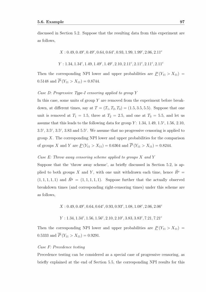
5.6. Example 97
discussed in Section 5.2. Suppose that the resulting data from this experiment are
as follows,
X : 0.49, 0.49c, 0.49c, 0.64, 0.64c, 0.93, 1.99, 1.99c, 2.06, 2.11c
Y : 1.34, 1.34c, 1.49, 1.49c, 1.49c, 2.10, 2.11c, 2.11c, 2.11c, 2.11c
Then the corresponding NPI lower and upper probabilities are P (Y11 > X11) =
0.5148 and P (Y11 > X11) = 0.8744.
Case D: Progressive Type-I censoring applied to group Y
In this case, some units of group Y are removed from the experiment before break-
down, at different times, say at T = (T1, T2, T3) = (1.5, 3.5, 5.5). Suppose that one
unit is removed at T1 = 1.5, three at T2 = 2.5, and one at T3 = 5.5, and let us
assume that this leads to the following data for group Y : 1.34, 1.49, 1.5c, 1.56, 2.10,
3.5c, 3.5c, 3.5c, 3.83 and 5.5c. We assume that no progressive censoring is applied to
group X. The corresponding NPI lower and upper probabilities for the comparison
of groups X and Y are P (Y11 > X11) = 0.6364 and P (Y11 > X11) = 0.8244.
Case E: Throw away censoring scheme applied to groups X and Y
Suppose that the ‘throw away scheme’, as briefly discussed in Section 5.2, is ap-
plied to both groups X and Y , with one unit withdrawn each time, hence Rx =
(1, 1, 1, 1, 1) and Ry = (1, 1, 1, 1, 1). Suppose further that the actually observed
breakdown times (and corresponding right-censoring times) under this scheme are
as follows,
X : 0.49, 0.49c, 0.64, 0.64c, 0.93, 0.93c, 1.08, 1.08c, 2.06, 2.06c
Y : 1.34, 1.34c, 1.56, 1.56c, 2.10, 2.10c, 3.83, 3.83c, 7.21, 7.21c
Then the corresponding NPI lower and upper probabilities are P (Y11 > X11) =
0.5333 and P (Y11 > X11) = 0.9291.
Case F: Precedence testing
Precedence testing can be considered as a special case of progressive censoring, as
briefly explained at the end of Section 5.5, the corresponding NPI results for this
5.7. Concluding remarks 98
approach are presented in Chapter 2. Suppose that the breakdown of insulating
fluids experiment is terminated as soon as the fifth breakdown from group Y is
observed, i.e. at time y5 = 2.12. Then the breakdown times of five units from group
Y are right-censored at that time, together with three units from group X. Then
P (Y11 > X11) = 0.5289 and P (Y11 > X11) = 0.8264.
Case G: Complete data
Let us end this example by considering NPI comparison of these two groups of
breakdown data using the complete data as presented in Table 5.1, so without
any (progressive) censoring scheme applied. NPI for such a comparison of complete
data from two groups was already presented by Coolen [19], and is also easily derived
from the results in this chapter by obvious choices for the censoring schemes, namely
Rxi = Ry
j = 0 for all i and j, and hence rx = nx and ry = ny. For this situation, the
NPI results are P (Y11 > X11) = 0.6364 and P (Y11 > X11) = 0.8099. 4
5.7 Concluding remarks
In this chapter, we introduced NPI for comparison of two groups of lifetime data
under several progressive censoring schemes. The NPI method has the attractive
feature that it is applicable whether progressive censoring is adopted for one group
or for both groups, and also for different censoring schemes. We have restricted
attention to two groups, but the methods presented here are quite easily generalized
to multiple groups, along the lines of the NPI methods for selection presented in
Chapters 3 and 4. Although the ideas for such a generalization are indeed straight-
forward, deriving analytical expressions of the corresponding NPI lower and upper
probabilities becomes somewhat tedious, it is more attractive to develop software
routines that perform such calculations for any specific M -functions specified per
group, and for any number of groups. In fact one can use the R commands provided
in the appendix of this thesis for such purposes since it can be used for comparison
of several groups and with different selection events of interest.
Chapter 6
Competing Risks
6.1 Introduction
In reliability, failure data often correspond to competing risks [13, 71], where several
failure modes can cause a unit to fail, and where failure occurs due to the first failure
event caused by one of the failure modes. Coolen et al. [23] introduced Nonparamet-
ric Predictive Inference (NPI) to some reliability applications, including lower and
upper survival functions for a future unit, illustrated with an application with com-
peting risks data. They illustrated the lower and upper marginal survival functions,
which are restricted to a single failure mode. In this chapter, the main question
considered is which failure mode will cause the next unit to fail, or for example in
survival analysis terminology, which disease causes the next individual considered to
die. From now on, terminology from reliability will be used, so events considered are
failures of units, but the methods proposed are of course more generally applicable.
In this chapter, NPI lower and upper probabilities are presented for the event
that a future unit, say unit n + 1, will fail due to a specific failure mode, based
on data consisting of times of failures resulting from competing risks for n units.
It also illustrates the effect of grouping different failure modes together, and some
special cases and features are discussed. This approach uses NPI for right-censored
data as presented by Coolen and Yan [27], see also Subsection 1.3.2. The use of
lower and upper probabilities to quantify uncertainty has gained increasing attention
during the last decade, short and detailed overviews of theories and applications in
99
6.2. Competing risks 100
reliability, together called ‘imprecise reliability’, are presented by Coolen and Utkin
[24, 74].
Some aspects of competing risks are briefly reviewed in Section 6.2. Section
6.3 presents NPI for the competing risks problem. In Section 6.4 we consider the
special case of two failure modes which leads to some interesting results. The NPI
method is illustrated by some examples in Section 6.5. NPI can also be applied
for different censoring mechanisms, which is illustrated in Section 6.6 for competing
risks inferences under progressive censoring. Some concluding remarks are given in
Section 6.7.
6.2 Competing risks
In competing risks, several failure modes can cause a unit to fail. Throughout this
chapter, we assume that each unit cannot fail more than once and it is not used any
further once it has failed, and that a failure is caused by a single failure mode which,
upon observing a failure, is known with certainty. Tsiatis [73] showed that failure
data resulting from such competing risks cannot be used to identify dependence
between the failure modes. Effectively, this means that such data can only be used
to learn about the marginal distributions, which are the distributions of failure
times restricted to single failure modes, for which all failures caused by other failure
modes lead to right-censored observations. Throughout this chapter we assume that
the failure modes are independent, inclusion of assumed dependence would be an
interesting topic for future research, but cannot be learned about from the data as
considered here as shown by Tsiatis, and NPI has also not yet been developed to
take dependence into account.
In this chapter, we consider competing risks, with k distinct failure modes that
can cause a unit to fail. It is further assumed that such failure observations are ob-
tained for n units. As is common in study of failure data under competing risks, for
each unit k random quantities are considered, say Tj for j = 1, . . . , k, where Tj repre-
sents the unit’s time to failure under the condition that failure occurs due to failure
mode j. These Tj are assumed to be independent continuous random quantities,
6.3. NPI for Competing Risks 101
which implies the assumption that the failure modes occur independently, and the
failure time of the unit is T = min(T1, . . . , Tk). Therefore, each unit considered can
have one failure time and it will be known with certainty which failure mode caused
a failure. Hence, for the Tj corresponding to the other failure modes, which did not
cause the failure of the unit, the unit’s observed failure time is a right-censoring
time.
In a sample of size n, suppose that there are q (q ≤ n) distinct failure times
x1 < x2 < . . . < xq. Let hij be the number of units that failed due to failure
mode j at time xi, and nxibe the number of units at risk at xi. Then, the marginal
distribution function of Tj, also called the Cumulative Incidence Function (CIF)[70],
Fj(t), can be estimated as
Fj(t) =∑
all i, xi≤t
hij
nxi
S(xi−1) (6.1)
where S(t) is the Kaplan-Meier (KM) estimator given by (1.7). For the case of
comparing two competing risks, i.e. two failure modes only, Kochar et al. [45] dis-
cussed several tests from literature to test whether the difference between the two
corresponding CIFs is different from zero.
In the competing risks literature (e.g. [30, 70]), one often consider a bivariate
random quantity (T,C), where C is an indicator which equals 0 if the observation
is censored and therefore T is the censoring time, or C = j where j represents the
failure mode that caused the failure, in which case T is the failure time due to failure
mode j [30]. NPI has not yet been developed for such bivariate random quantities,
which is an interesting challenge for future research.
6.3 NPI for Competing Risks
For the NPI approach, let the failure time of a future unit be denoted by Xn+1, and
let the corresponding notation for the failure time including indication of the actual
failure mode, say failure mode j, be Xj,n+1 (so Xn+1 corresponds to an observation
T for unit n+1, and Xj,n+1 to Tj , according to the notation in the previous section).
As the different failure modes are assumed to occur independently, the competing
6.3. NPI for Competing Risks 102
risk data per failure mode consist of a number of observed failure times for failures
caused by the specific failure mode considered, and right-censoring times for failures
caused by other failure modes. Hence rc-A(n) can be applied per failure mode j,
for inference on Xj,n+1. Let the number of failures caused by failure mode j be uj,
xj,1 < xj,2 < . . . < xj,uj, and let υj(= n − uj) be the number of the right-censored
observations, cj,1 < cj,2 < . . . < cj,υj , corresponding to failure mode j. Again we
assume that no ties occur, however we deal with ties as discussed in Subsection
1.3.5. For notational convenience, let xj,0 = 0 and xj,uj+1 = ∞. Suppose further
that there are sj,ij right-censored observations in the interval (xj,ij , xj,ij+1), denoted
by cijj,1 < c
ijj,2 < . . . < c
ijj,sj,ij
, so∑uj
ij=0 sj,ij = υj. It should be emphasized that it is not
assumed that each of the n units in the data set actually has failed. If a unit has not
failed then there will be a right-censored observation recorded for this unit for each
failure mode, as it is assumed that the unit will then be withdrawn from the study,
or the study ends, at some point. The random quantity representing the failure time
of the next unit, with all k failure modes considered, is Xn+1 = min1≤j≤k
Xj,n+1. Before
introducing the NPI lower and upper probabilities for the event of interest, the NPI
M -function values for Xj,n+1 (j = 1, . . . , k) following from Definition 1.2, are given
below.
Definition 6.1. The NPI M -functions for Xj,n+1 (j = 1, . . . , k) are
M j(tijj,i∗j
, xj,ij+1) = MXj,nj+1(t
ijj,i∗j
, xj,ij+1) =1
n+1(n
tij
j,i∗j
)δij
i∗j−1 ∏
r:cj,r<tij
j,i∗j
ncj,r+1
ncj,r
(6.2)
where ij = 0, 1, . . . , uj , i∗j = 0, 1, . . . , sj,ij and
δiji∗j=
1 if i∗j = 0 i.e. tijj,0 = xj,ij (failure time or time 0)
0 if i∗j = 1, . . . , sj,ij i.e. tijj,i∗j
= cijj,i∗j
(censoring time)
Again ncr and ntij
j,i∗j
are the numbers of units in the risk set just prior to times cr
and tijj,i∗j
, respectively. The corresponding NPI probabilities are
P j(xj,ij , xj,ij+1) = P (Xj,nj+1 ∈ (xj,ij , xj,ij+1)) =1
n+ 1
∏
r:cj,r<xj,ij+1
ncj,r + 1
ncj,r
(6.3)
where xj,ij and xj,ij+1 are two consecutive observed failure times caused by failure
mode j (and xj,0 = 0, xj,uj+1 = ∞).
6.3. NPI for Competing Risks 103
In this chapter, the main event of interest is that a single future unit, called the
‘next unit’, undergoing the same test or process as the n units for which failure data
are available, fails due to a specific failure mode, say mode l. NPI lower and upper
probabilities for this event are derived, for each l = 1, . . . , k. The following notation
is used for these NPI lower and upper probabilities, respectively, for the event of
interest.
P (l) = P
(
Xl,n+1 = min1≤j≤k
Xj,n+1
)
= P
Xl,n+1 < min1≤j≤k
j 6=l
Xj,n+1
P(l)
= P
(
Xl,n+1 = min1≤j≤k
Xj,n+1
)
= P
Xl,n+1 < min1≤j≤k
j 6=l
Xj,n+1
These NPI lower and upper probabilities for the event of interest are presented in
the following theorem.
Theorem 6.1. The NPI lower and upper probabilities for the event that the next
unit will fail due to failure mode l are
P (l) =∑∑∑∑∑∑
Cl(j, ij , i∗j )
ul∑
il=0
1xl,il+1< min1≤j≤k
j 6=l
tijj,i∗jPl(xl,il , xl,il+1)
k∏
j=1
j 6=l
M j(tijj,i∗j
, xj,ij+1) (6.4)
P(l)
=∑∑∑∑∑∑
Cl(j, ij)
ul∑
il=0
sl,il∑
i∗l=0
1till,i∗l< min
1≤j≤k
j 6=l
xj,ij+1M l(till,i∗l, xl,il+1)
k∏
j=1
j 6=l
P j(xj,ij , xj,ij+1) (6.5)
where∑∑∑∑∑∑
Cl(j, ij , i∗j )
denotes the sums over all i∗j from 0 to sj,ij and over all ij from 0 to
uj for j = 1, . . . , k but not including j = l. Similarly,∑∑∑∑∑∑
Cl(j, ij)
denotes the sums over
all ij from 0 to uj for j = 1, . . . , k but not including j = l.
Proof. The NPI lower and upper probabilities (6.4) and (6.5) are derived as the
sharpest bounds, based on the relevant rc-A(n) assumptions, for the probability
P=P
Xl,n+1< min1≤j≤k
j 6=l
Xj,n+1
=∑∑∑∑∑∑
Cl(j, ij)
P
Xl,n+1< min1≤j≤k
j 6=l
Xj,n+1,k⋂
j=1
j 6=l
Xj,n+1∈(xj,ij , xj,ij+1)
6.4. Two competing risks 104
First consider the lower probability (6.4), which is derived as the sharpest general
lower bound for the above probability P ,
P ≥∑∑∑∑∑∑
Cl(j, ij , i∗j )
P
Xl,n+1 < min1≤j≤k
j 6=l
tijj,i∗j
.
k∏
j=1
j 6=l
M j(tijj,i∗j
, xj,ij+1)
≥∑∑∑∑∑∑
Cl(j, ij , i∗j )
ul∑
il=0
1xl,il+1 < min1≤j≤k
j 6=l
tijj,i∗jPl(xl,il , xl,il+1)
k∏
j=1
j 6=l
M j(tijj,i∗j
, xj,ij+1)
The first inequality follows by putting all probability masses for each Xj,n+1 (j =
1, . . . , k and j 6= l) assigned to the intervals (tijj,i∗j
, xj,ij+1) (ij = 0, . . . , uj and i∗j =
0, 1, . . . , sj,ij) at the left end points of these intervals, and by using Lemma 1.4 for
the nested intervals. The second inequality follows by putting all probability masses
for Xl,n+1 in each of the intervals (till,i∗l, xl,il+1) (il = 0, . . . , ul and i∗l = 0, 1, . . . , sl,il)
at the right end points of these intervals. The upper probability is obtained in a
similar way, but now all probability masses for the random quantities involved are
put at the opposite end points of the respective intervals, when compared to the
derivation of the lower probability which leads to
P ≤∑∑∑∑∑∑
Cl(j, ij)
P
Xl,n+1 < min1≤j≤k
j 6=l
xj,ij+1
k∏
j=1
j 6=l
P j(xj,ij , xj,ij+1)
≤∑∑∑∑∑∑
Cl(j, ij)
ul∑
il=0
sl,il∑
i∗l=0
1till,i∗l< min
1≤j≤k
j 6=l
xj,ij+1M l(till,i∗l, xl,il+1)
k∏
j=1
j 6=l
P j(xj,ij , xj,ij+1)
6.4 Two competing risks
Before illustrating and discussing this method in examples in Section 6.5, let us
consider the special case of the competing risks problem in which there are only
two failure modes (so k = 2), say modes l and j, and in which each of the n units
considered actually fails due to one of these two failure modes. Therefore, any unit
which fails due to failure mode l leads to a right-censored observation for failure
mode j, and vice versa. In this case, the number of failures due to failure mode l
6.4. Two competing risks 105
(j) is equal to the number of right-censored observations for failure mode j (l), so
υl = uj and υj = ul. Let Rl (Rj) be the set of ranks of all ordered failure times due
to failure mode l (j), so Rl ⊂ 1, 2, . . . , n and Rj = 1, 2, . . . , n \ Rl. The NPI
lower and upper probabilities for this scenario are presented in Theorem 6.2.
Theorem 6.2. The NPI lower and upper probabilities (6.4) and (6.5) for the event
that the next unit will fail due to failure mode l, in case of only two failure modes,
l and j, are
P (l) =1
n+ 1
∑
rl∈Rl
nxl,(rl)
nxl,(rl)+ 1
=1
n+ 1
∑
rl∈Rl
n+ 1− rln+ 2− rl
(6.6)
P(l)
= 1− 1
n+ 1
∑
rj∈Rj
nxj,(rj)
nxj,(rj)+ 1
= 1− 1
n+ 1
∑
rj∈Rj
n+ 1− rjn+ 2− rj
(6.7)
Proof. In the case of two competing risks, the NPI lower probability (6.4), i.e. P (l) =
P (Xl,nl+1 < Xj,nj+1), becomes
P (l) =
uj∑
ij=0
sj,ij∑
i∗j=0
ul∑
il=0
1xl,il+1 < tijj,i∗j
P l(xl,il , xl,il+1)
M j(tijj,i∗j
, xj,ij+1) (6.8)
Above we have assumed that all n units considered have actually failed due to one
of these two failure modes. As any failure of a unit due to failure mode l leads to
a right-censored observation for failure mode j for that unit, and vice versa, then
xl,(rl) = cj,(rl) (xj,(rj) = cl,(rj)) for rl ∈ Rl (rj ∈ Rj). Let∑∑∑∑∑∑
C(ij ,i∗j ,cj,(rl))
denote the sums
over all ij from 0 to uj and over all i∗j from 0 to sj,ij such that tijj,i∗j
≥ cj,(rl). Then
the NPI lower probability (6.8) can be written as
P (l) =∑
rl∈Rl
P l(xl,(rl−1), xl,(rl))∑∑∑∑∑∑
C(ij ,i∗j ,cj,(rl))
M j(tijj,i∗j
, xj,ij+1)
=∑
rl∈Rl
P l(xl,(rl−1), xl,(rl)) SXj,n+1(cj,(rl))
=∑
rl∈Rl
(
1
n+ 1
∏
r:cl,r<xl,(rl)
ncl,r + 1
ncl,r
)(
1
n+ 1ncj,(rl)
∏
r:cj,r<cj,(rl)
ncj,r + 1
ncj,r
)
=∑
rl∈Rl
(
1
n+ 1
)2(n+ 1
n+ 2− rl
)
(n+ 1− rl)
=1
n+ 1
∑
rl∈Rl
n+ 1− rln+ 2− rl
.
6.4. Two competing risks 106
The second equality and the second term in the third equality follow immediately
from the definition of the lower survival function [23] and its simplest closed-form
(1.11) derived in Chapter 1, respectively. The fourth equality in this derivation
results from the fact that, with all units assumed to fail due to one of the two failure
modes considered, and xl,(rl) = cj,(rl) and xj,(rj) = cl,(rj) for all rl ∈ Rl and rj ∈ Rj,
the two product terms combine into a single product over all first rl−1 observations.
This product simplifies to n+1n+2−rl
, and ncj,(rl)= n+1− rl completes the justification
of the fourth equality.
The corresponding NPI upper probability (6.7) can be derived similarly, but it is
easier to do so by use of the conjugacy property, P(l)
= 1− P (Xl,nl+1 > Xj,nj+1) =
1− P (j) where
P (j) =1
n+ 1
∑
rj∈Rj
n+ 1− rjn+ 2− rj
is of course obtained directly from the above expression for P (l).
Furthermore, the imprecision for the event considered here, in this special case of
competing risks with only two failure modes and all n units actually having failed,
does not depend on the number of failures caused by each failure mode nor on their
ordering. This is implied by the following theorem.
Theorem 6.3. The imprecision for the above scenario is equal to
Imprecision = P(l) − P (l) =
1
n+ 1
n+1∑
i=1
1
i
Proof. For this situation with two failure modes and all n units failing due to one
of them, the imprecision is
Imprecision = 1−
P (l) + P (j)
= 1− 1
n+ 1
∑
rl∈Rl
n+ 1− rln+ 2− rl
+∑
rj∈Rj
n+ 1− rjn+ 2− rj
= 1− 1
n+ 1
n∑
i=1
n+ 1− i
n+ 2− i
=1
n+ 1
[
1 +n∑
i=1
1
n+ 2− i
]
=1
n+ 1
n+1∑
i=1
1
i.
The second equality follows directly from Theorem 6.2.
6.4. Two competing risks 107
It should be emphasized that these attractive properties of the NPI results in
the case of two competing risks do not generalize to more than two competing risks,
due to the fact that the product terms in the NPI lower and upper probabilities
(6.4) and (6.5) only disappear for this case with two failure modes and all n units
actually having failed.
The formulae (6.6) and (6.7) enable the derivation of some interesting results
of the NPI approach in this specific setting, with only two failure modes and all n
units actually having failed. Consider the following two specific scenarios in detail:
(A) all failures due to failure mode j come first, followed by all failures from failure
mode l, meaning that the uj failure times of failures due to mode j are all smaller
than the ul failure times of failures due to mode l. In this case, the NPI lower and
upper probabilities for the event that the next unit will fail due to failure mode l
are
P (l), A =1
n+ 1
ul∑
i=1
i
i+ 1and P
(l), A= 1− 1
n+ 1
n∑
i=ul+1
i
i+ 1
(B) all failures due to failure mode l come first, followed by all failures from failure
mode j, in which case the NPI lower and upper probabilities for the event of interest
are
P (l), B =1
n+ 1
n∑
i=uj+1
i
i+ 1and P
(l), B= 1− 1
n+ 1
uj∑
i=1
i
i+ 1
These NPI lower and upper probabilities follow straightforwardly from the general
expressions (6.6) and (6.7) for these two special cases. Because ii+1
is increasing in
i, these results imply that case (A) leads to the minimal NPI lower and upper prob-
abilities when all possible orderings of uj failures due to mode j and ul failures due
to mode l are considered, while case (B) leads to the maximal NPI lower and upper
probabilities in this setting. More generally, these results imply a nice monotonicity
result, namely that the NPI lower and upper probabilities (6.6) and (6.7) increase
whenever any failure caused by failure mode l would move to an earlier place in the
ordering. This is illustrated in Example 6.1 in Section 6.5.
6.5. Examples 108
6.5 Examples
In this section three examples of NPI for competing risks are presented to illustrate
the method and to discuss some of its properties. Example 6.1 is a small example
which serves to illustrate the results presented in Section 6.4. Examples 6.2 and
6.3 involve a substantial competing risks data set from the literature, with different
groupings of failure modes and also including some units which did not fail at all
during the study, hence leading to right-censored observations for each of the failure
modes considered. This will illustrate a further important aspect of NPI in this
setting, and will also lead to a conjecture.
Example 6.1. Consider an experiment in which five units are subjected to two
failure modes, FM1 and FM2, which are competing risks in the manner discussed
in this chapter. Suppose that all five units are observed to fail, and that three units
fail due to FM1 and two units due to FM2. So the failure times of the three units
failing due to FM1 are right-censored observations for FM2, and the failure times of
the two units which fail due to FM2 are right-censored observations for FM1. As all
five units actually fail during the experiment, no further right-censored observations
occur in this example. Suppose that there had actually been a sixth unit in the
experiment, and this was randomly selected before the start of the experiment as
the unit for which the failure information would not be revealed to us. The method
presented in this chapter provides inferences for the event that this sixth unit fails
due to FM1 or due to FM2 (instead ’will fail’ could be used, if the inferences are
interpreted as involving a future unit undergoing the same experiment, both are
convenient ways to think about the setting and inferences).
In this NPI approach, the actual failure times of the five units are not important,
only their ordering with regard to failure modes is important. Of course, NPI can
also be used for inference on the actual failure time of the sixth unit, for example
by considering the event that this unit will not fail before a specified time, in which
case the failure times of the five units are explicitly used, not only their ordering
with regard to the failure modes, this is briefly illustrated for Examples 6.2 and 6.3
at the end of this section. There are 10 possible orderings for the failure modes FM1
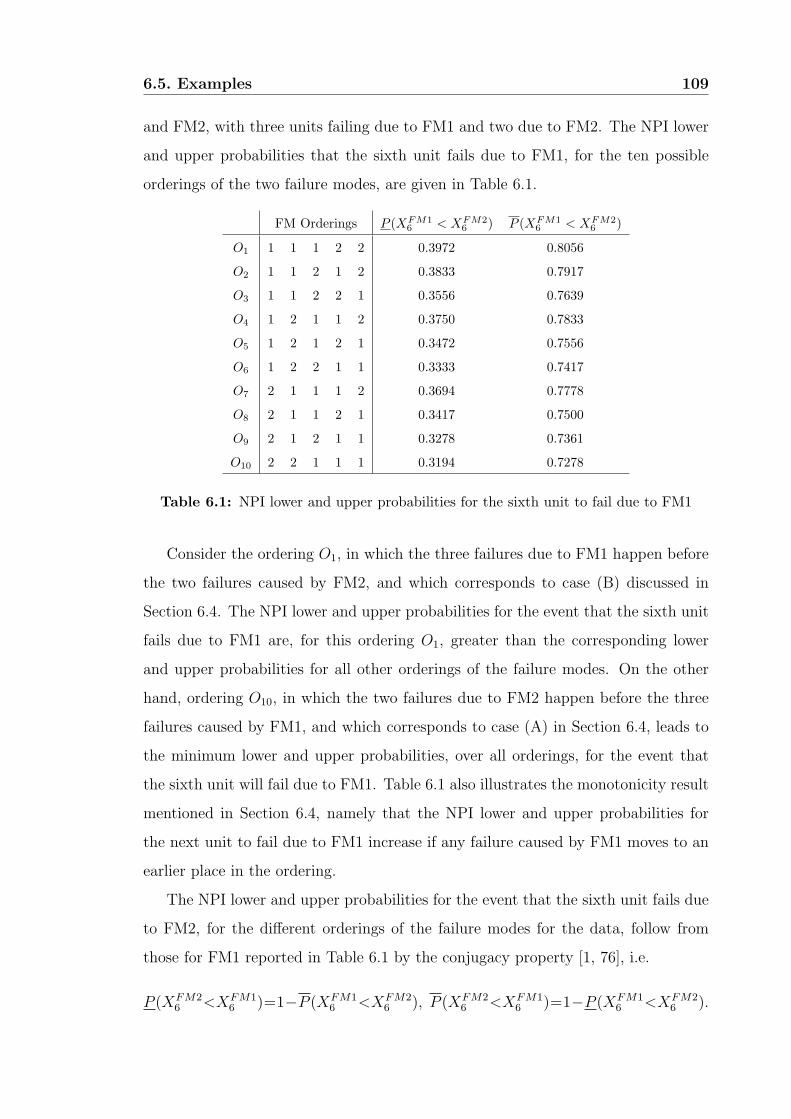
6.5. Examples 109
and FM2, with three units failing due to FM1 and two due to FM2. The NPI lower
and upper probabilities that the sixth unit fails due to FM1, for the ten possible
orderings of the two failure modes, are given in Table 6.1.
FM Orderings P (XFM16 < XFM2
6 ) P (XFM16 < XFM2
6 )
O1 1 1 1 2 2 0.3972 0.8056
O2 1 1 2 1 2 0.3833 0.7917
O3 1 1 2 2 1 0.3556 0.7639
O4 1 2 1 1 2 0.3750 0.7833
O5 1 2 1 2 1 0.3472 0.7556
O6 1 2 2 1 1 0.3333 0.7417
O7 2 1 1 1 2 0.3694 0.7778
O8 2 1 1 2 1 0.3417 0.7500
O9 2 1 2 1 1 0.3278 0.7361
O10 2 2 1 1 1 0.3194 0.7278
Table 6.1: NPI lower and upper probabilities for the sixth unit to fail due to FM1
Consider the ordering O1, in which the three failures due to FM1 happen before
the two failures caused by FM2, and which corresponds to case (B) discussed in
Section 6.4. The NPI lower and upper probabilities for the event that the sixth unit
fails due to FM1 are, for this ordering O1, greater than the corresponding lower
and upper probabilities for all other orderings of the failure modes. On the other
hand, ordering O10, in which the two failures due to FM2 happen before the three
failures caused by FM1, and which corresponds to case (A) in Section 6.4, leads to
the minimum lower and upper probabilities, over all orderings, for the event that
the sixth unit will fail due to FM1. Table 6.1 also illustrates the monotonicity result
mentioned in Section 6.4, namely that the NPI lower and upper probabilities for
the next unit to fail due to FM1 increase if any failure caused by FM1 moves to an
earlier place in the ordering.
The NPI lower and upper probabilities for the event that the sixth unit fails due
to FM2, for the different orderings of the failure modes for the data, follow from
those for FM1 reported in Table 6.1 by the conjugacy property [1, 76], i.e.
P (XFM26 <XFM1
6 )=1−P (XFM16 <XFM2
6 ), P (XFM26 <XFM1
6 )=1−P (XFM16 <XFM2
6 ).
6.5. Examples 110
Consider, for example, the ordering O5, for which the corresponding NPI lower and
upper probabilities that the sixth unit fails due to FM1 are 0.3472 and 0.7556, while
for this unit to fail due to FM2 they are 0.2444 and 0.6528. On the basis of these
NPI lower and upper probabilities alone, one could conclude that there is a weak
indication that failure due to FM1 is more likely than due to FM2, as
P (XFM16 < XFM2
6 ) = 0.3472 > 0.2444 = P (XFM26 < XFM1
6 )
and
P (XFM16 < XFM2
6 ) = 0.7556 > 0.6528 = P (XFM26 < XFM1
6 )
One could speak about a strong indication for the event that failure of the sixth
unit will be caused by FM1 if P (XFM16 < XFM2
6 ) > P (XFM26 < XFM1
6 ), which does
not occur for any of the orderings in this example. Finally, the imprecision in this
example, for all orderings of the two failure modes, is equal to 0.4084, illustrating
the property presented in Theorem 6.3. 4
Example 6.2. In this example and in Example 6.3, a well-known data set from the
literature [48] is used to illustrate some aspects of the NPI method for dealing with
competing risks. The data contain information about 36 units of a new model of a
small electrical appliance which were tested, and where the lifetime observation per
unit consists of the number of completed cycles of use until the unit failed. These
data are presented in Table 6.2, which also includes the specific failure mode (FM)
that caused the unit to fail. In the study, there were 18 different ways in which
an appliance could fail, so 18 failure modes, but to illustrate the NPI method this
number is reduce to two (groups of) failure modes in the current example, while
grouping into three failure modes is considered in Example 6.3, after which the
differences between these examples are discussed. Three units in the test did not
fail before the end of the experiment, so for these units right-censored observations
(2565, 6367 and 13403) are recorded for all failure modes considered, indicated by
‘-’ for the failure mode in Table 6.2.
The two most frequently occurring failure modes in these data are FM9, which
caused 17 units to fail, and FM6 which caused 7 failures. It is considered how likely
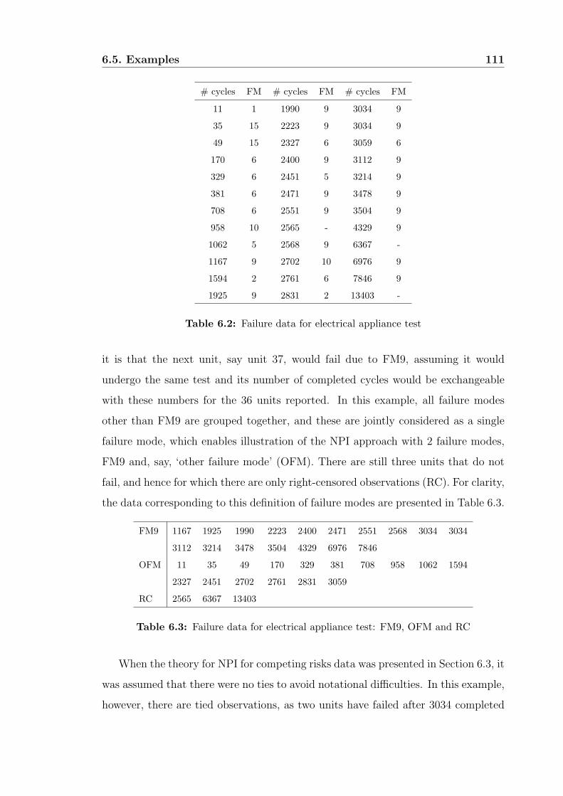
6.5. Examples 111
# cycles FM # cycles FM # cycles FM
11 1 1990 9 3034 9
35 15 2223 9 3034 9
49 15 2327 6 3059 6
170 6 2400 9 3112 9
329 6 2451 5 3214 9
381 6 2471 9 3478 9
708 6 2551 9 3504 9
958 10 2565 - 4329 9
1062 5 2568 9 6367 -
1167 9 2702 10 6976 9
1594 2 2761 6 7846 9
1925 9 2831 2 13403 -
Table 6.2: Failure data for electrical appliance test
it is that the next unit, say unit 37, would fail due to FM9, assuming it would
undergo the same test and its number of completed cycles would be exchangeable
with these numbers for the 36 units reported. In this example, all failure modes
other than FM9 are grouped together, and these are jointly considered as a single
failure mode, which enables illustration of the NPI approach with 2 failure modes,
FM9 and, say, ‘other failure mode’ (OFM). There are still three units that do not
fail, and hence for which there are only right-censored observations (RC). For clarity,
the data corresponding to this definition of failure modes are presented in Table 6.3.
FM9 1167 1925 1990 2223 2400 2471 2551 2568 3034 3034
3112 3214 3478 3504 4329 6976 7846
OFM 11 35 49 170 329 381 708 958 1062 1594
2327 2451 2702 2761 2831 3059
RC 2565 6367 13403
Table 6.3: Failure data for electrical appliance test: FM9, OFM and RC
When the theory for NPI for competing risks data was presented in Section 6.3, it
was assumed that there were no ties to avoid notational difficulties. In this example,
however, there are tied observations, as two units have failed after 3034 completed
6.5. Examples 112
cycles, both failed due to FM9. To deal with this, it is assumed that there is a
small difference between these values, such that their ordering does not change with
regard to observations of units in other groups. It is actually assumed that one
of these two units failed after 3035 completed cycles. Implicit in the NPI method
for competing risks data is that a failure time observation caused by one failure
mode is simultaneously a right-censored observation for all other failure modes.
This situation is dealt with in the NPI approach, as is common in many statistical
approaches, by assuming that the right-censoring time is just beyond the failure
time. The three right-censored observations, for units that were not observed to
fail during the experiment, also lead to tied observations for the two failure modes
(FM9 and OFM) considered, as for both the right-censoring times coincide. This is
also dealt with by assuming that for one of the failure modes this event occurred
fractionally later than for the other failure mode, and then the lower and upper
probabilities for the event of interest are calculated by considering the minimum
and maximum of the lower and upper probabilities, respectively, corresponding to
the different possible orderings of these ‘un-tied’ right-censoring times.
The NPI lower and upper probabilities for the event that unit 37 will fail due to
FM9 are
P (XFM937 < XOFM
37 ) = 0.4358 , P (XFM937 < XOFM
37 ) = 0.5804
while the corresponding NPI lower and upper probabilities for unit 37 to fail due to
OFM are
P (XOFM37 < XFM9
37 ) = 0.4196 , P (XOFM37 < XFM9
37 ) = 0.5642
These lower and upper probabilities satisfy the conjugacy property [1, 76], which is
due to the fact that, implicit in our method, it is assumed that the experiment on
unit 37 would actually continue until it fails, and this is assumed to happen with
certainty. On the basis of these NPI lower and upper probabilities, the data could
be considered to contain a weak indication that the event that unit 37 will fail due
to FM9 is a bit more likely than for it to fail due to another failure mode, with all
the other failure modes grouped together as done in this example. 4
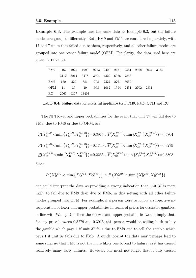
6.5. Examples 113
Example 6.3. This example uses the same data as Example 6.2, but the failure
modes are grouped differently. Both FM9 and FM6 are considered separately, with
17 and 7 units that failed due to them, respectively, and all other failure modes are
grouped into one ‘other failure mode’ (OFM). For clarity, the data used here are
given in Table 6.4.
FM9 1167 1925 1990 2223 2400 2471 2551 2568 3034 3034
3112 3214 3478 3504 4329 6976 7846
FM6 170 329 381 708 2327 2761 3059
OFM 11 35 49 958 1062 1594 2451 2702 2831
RC 2565 6367 13403
Table 6.4: Failure data for electrical appliance test: FM9, FM6, OFM and RC
The NPI lower and upper probabilities for the event that unit 37 will fail due to
FM9, due to FM6 or due to OFM, are
P(
XFM937 <min
XFM637 , XOFM
37
)
=0.3915 , P(
XFM937 <min
XFM637 , XOFM
37
)
=0.5804
P(
XFM637 <min
XFM937 , XOFM
37
)
=0.1749 , P(
XFM637 <min
XFM937 , XOFM
37
)
=0.3279
P(
XOFM37 <min
XFM637 , XFM9
37
)
=0.2265 , P(
XOFM37 <min
XFM637 , XFM9
37
)
=0.3808
Since
P(
XFM937 < min
XFM637 , XOFM
37
)
> P(
XFM637 < min
XFM937 , XOFM
37
)
one could interpret the data as providing a strong indication that unit 37 is more
likely to fail due to FM9 than due to FM6, in this setting with all other failure
modes grouped into OFM. For example, if a person were to follow a subjective in-
terpretation of lower and upper probabilities in terms of prices for desirable gambles,
in line with Walley [76], then these lower and upper probabilities would imply that,
for any price between 0.3279 and 0.3915, this person would be willing both to buy
the gamble which pays 1 if unit 37 fails due to FM9 and to sell the gamble which
pays 1 if unit 37 fails due to FM6. A quick look at the data may perhaps lead to
some surprise that FM6 is not the more likely one to lead to failure, as it has caused
relatively many early failures. However, one must not forget that it only caused
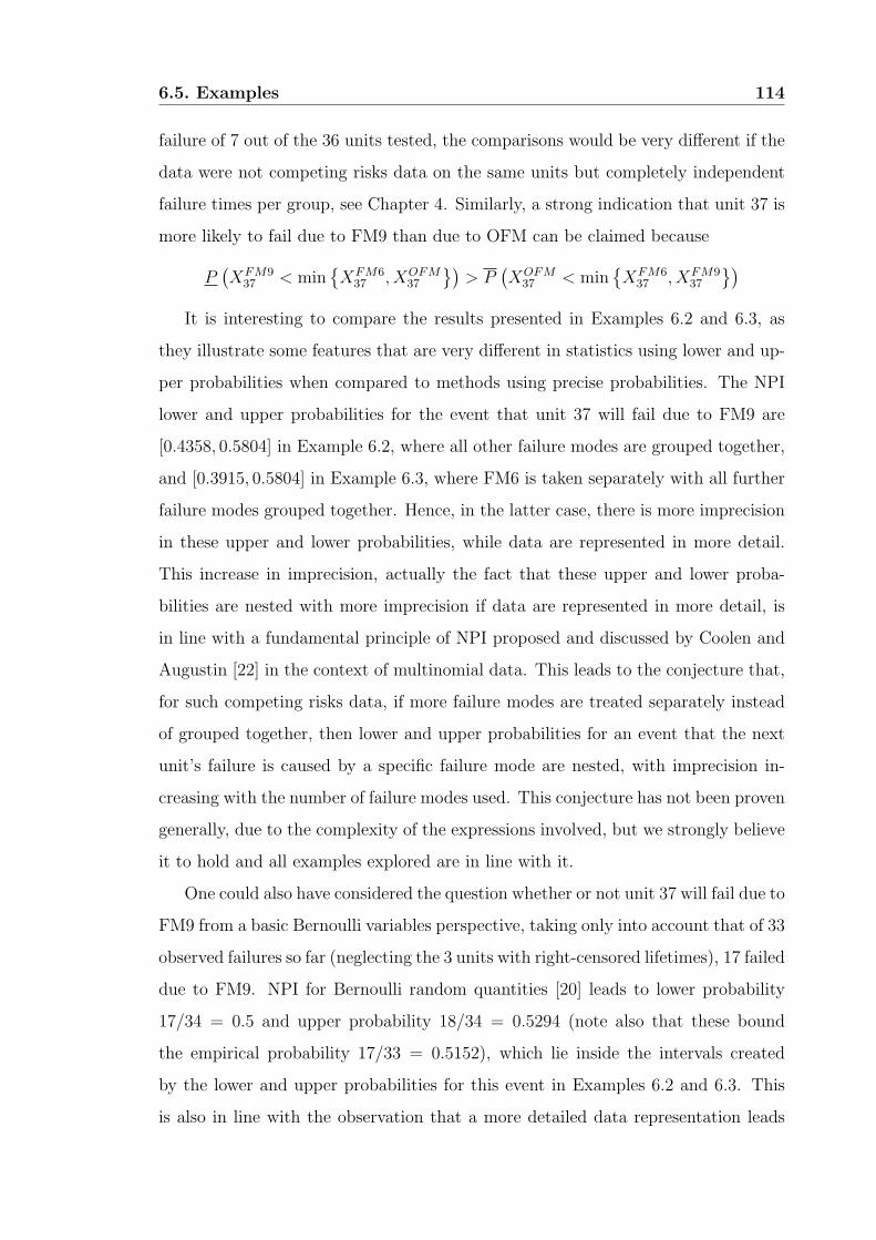
6.5. Examples 114
failure of 7 out of the 36 units tested, the comparisons would be very different if the
data were not competing risks data on the same units but completely independent
failure times per group, see Chapter 4. Similarly, a strong indication that unit 37 is
more likely to fail due to FM9 than due to OFM can be claimed because
P(
XFM937 < min
XFM637 , XOFM
37
)
> P(
XOFM37 < min
XFM637 , XFM9
37
)
It is interesting to compare the results presented in Examples 6.2 and 6.3, as
they illustrate some features that are very different in statistics using lower and up-
per probabilities when compared to methods using precise probabilities. The NPI
lower and upper probabilities for the event that unit 37 will fail due to FM9 are
[0.4358, 0.5804] in Example 6.2, where all other failure modes are grouped together,
and [0.3915, 0.5804] in Example 6.3, where FM6 is taken separately with all further
failure modes grouped together. Hence, in the latter case, there is more imprecision
in these upper and lower probabilities, while data are represented in more detail.
This increase in imprecision, actually the fact that these upper and lower proba-
bilities are nested with more imprecision if data are represented in more detail, is
in line with a fundamental principle of NPI proposed and discussed by Coolen and
Augustin [22] in the context of multinomial data. This leads to the conjecture that,
for such competing risks data, if more failure modes are treated separately instead
of grouped together, then lower and upper probabilities for an event that the next
unit’s failure is caused by a specific failure mode are nested, with imprecision in-
creasing with the number of failure modes used. This conjecture has not been proven
generally, due to the complexity of the expressions involved, but we strongly believe
it to hold and all examples explored are in line with it.
One could also have considered the question whether or not unit 37 will fail due to
FM9 from a basic Bernoulli variables perspective, taking only into account that of 33
observed failures so far (neglecting the 3 units with right-censored lifetimes), 17 failed
due to FM9. NPI for Bernoulli random quantities [20] leads to lower probability
17/34 = 0.5 and upper probability 18/34 = 0.5294 (note also that these bound
the empirical probability 17/33 = 0.5152), which lie inside the intervals created
by the lower and upper probabilities for this event in Examples 6.2 and 6.3. This
is also in line with the observation that a more detailed data representation leads
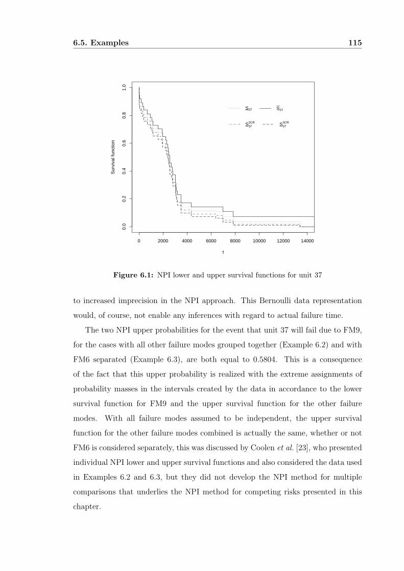
6.5. Examples 115
0 2000 4000 6000 8000 10000 12000 14000
0.0
0.2
0.4
0.6
0.8
1.0
t
Sur
viva
l fun
ctio
nS37 S37
S372CR S37
3CR
Figure 6.1: NPI lower and upper survival functions for unit 37
to increased imprecision in the NPI approach. This Bernoulli data representation
would, of course, not enable any inferences with regard to actual failure time.
The two NPI upper probabilities for the event that unit 37 will fail due to FM9,
for the cases with all other failure modes grouped together (Example 6.2) and with
FM6 separated (Example 6.3), are both equal to 0.5804. This is a consequence
of the fact that this upper probability is realized with the extreme assignments of
probability masses in the intervals created by the data in accordance to the lower
survival function for FM9 and the upper survival function for the other failure
modes. With all failure modes assumed to be independent, the upper survival
function for the other failure modes combined is actually the same, whether or not
FM6 is considered separately, this was discussed by Coolen et al. [23], who presented
individual NPI lower and upper survival functions and also considered the data used
in Examples 6.2 and 6.3, but they did not develop the NPI method for multiple
comparisons that underlies the NPI method for competing risks presented in this
chapter.
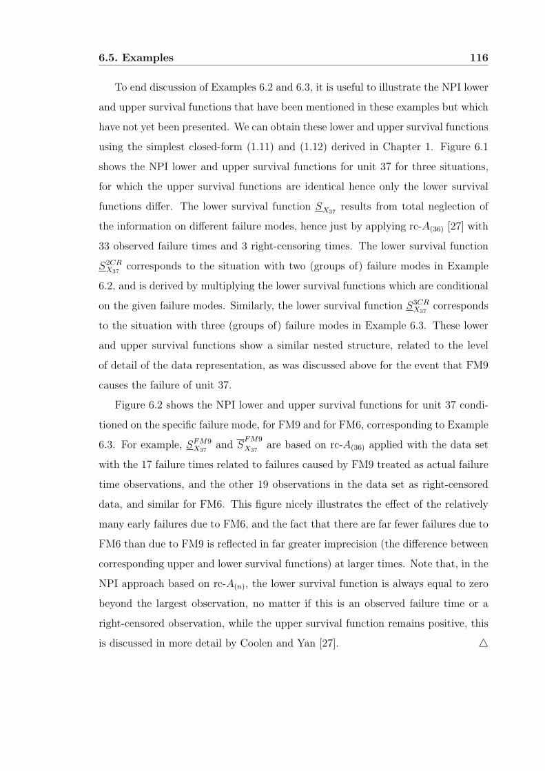
6.5. Examples 116
To end discussion of Examples 6.2 and 6.3, it is useful to illustrate the NPI lower
and upper survival functions that have been mentioned in these examples but which
have not yet been presented. We can obtain these lower and upper survival functions
using the simplest closed-form (1.11) and (1.12) derived in Chapter 1. Figure 6.1
shows the NPI lower and upper survival functions for unit 37 for three situations,
for which the upper survival functions are identical hence only the lower survival
functions differ. The lower survival function SX37results from total neglection of
the information on different failure modes, hence just by applying rc-A(36) [27] with
33 observed failure times and 3 right-censoring times. The lower survival function
S2CRX37
corresponds to the situation with two (groups of) failure modes in Example
6.2, and is derived by multiplying the lower survival functions which are conditional
on the given failure modes. Similarly, the lower survival function S3CRX37
corresponds
to the situation with three (groups of) failure modes in Example 6.3. These lower
and upper survival functions show a similar nested structure, related to the level
of detail of the data representation, as was discussed above for the event that FM9
causes the failure of unit 37.
Figure 6.2 shows the NPI lower and upper survival functions for unit 37 condi-
tioned on the specific failure mode, for FM9 and for FM6, corresponding to Example
6.3. For example, SFM9X37
and SFM9
X37are based on rc-A(36) applied with the data set
with the 17 failure times related to failures caused by FM9 treated as actual failure
time observations, and the other 19 observations in the data set as right-censored
data, and similar for FM6. This figure nicely illustrates the effect of the relatively
many early failures due to FM6, and the fact that there are far fewer failures due to
FM6 than due to FM9 is reflected in far greater imprecision (the difference between
corresponding upper and lower survival functions) at larger times. Note that, in the
NPI approach based on rc-A(n), the lower survival function is always equal to zero
beyond the largest observation, no matter if this is an observed failure time or a
right-censored observation, while the upper survival function remains positive, this
is discussed in more detail by Coolen and Yan [27]. 4
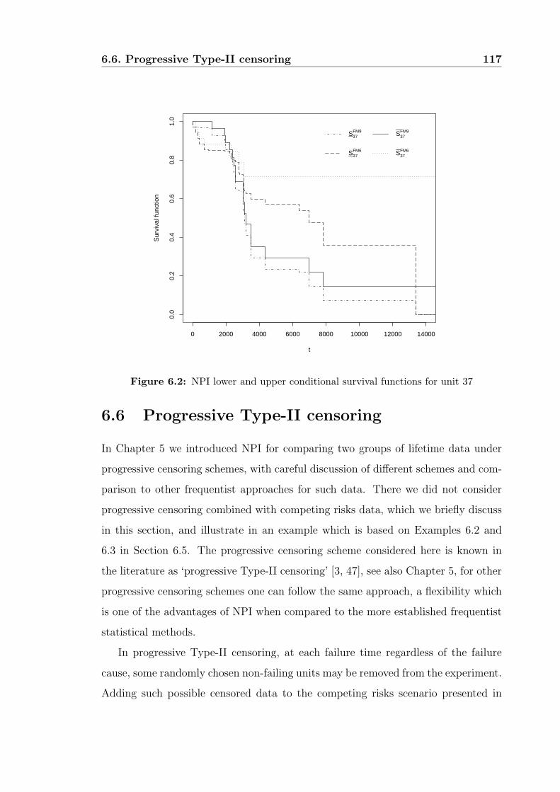
6.6. Progressive Type-II censoring 117
0 2000 4000 6000 8000 10000 12000 14000
0.0
0.2
0.4
0.6
0.8
1.0
t
Sur
viva
l fun
ctio
n
S37FM9 S37
FM9
S37FM6 S37
FM6
Figure 6.2: NPI lower and upper conditional survival functions for unit 37
6.6 Progressive Type-II censoring
In Chapter 5 we introduced NPI for comparing two groups of lifetime data under
progressive censoring schemes, with careful discussion of different schemes and com-
parison to other frequentist approaches for such data. There we did not consider
progressive censoring combined with competing risks data, which we briefly discuss
in this section, and illustrate in an example which is based on Examples 6.2 and
6.3 in Section 6.5. The progressive censoring scheme considered here is known in
the literature as ‘progressive Type-II censoring’ [3, 47], see also Chapter 5, for other
progressive censoring schemes one can follow the same approach, a flexibility which
is one of the advantages of NPI when compared to the more established frequentist
statistical methods.
In progressive Type-II censoring, at each failure time regardless of the failure
cause, some randomly chosen non-failing units may be removed from the experiment.
Adding such possible censored data to the competing risks scenario presented in
6.6. Progressive Type-II censoring 118
this chapter, the competing risks data per failure mode can consist of a number
of observed failures caused by the specific failure mode considered, right-censored
observations for failures caused by other failure modes, right-censored observations
resulting from removing some non-failing units at failure times of other units (due
to the progressive censoring scheme), and general right-censored observations due to
unknown failure modes or other reasons, as was also allowed earlier in this chapter.
The key thing here is that right-censored data of any kind are dealt with in the
same manner, per failure mode, in NPI for competing risks, so effectively there is no
difference in the way NPI for competing risks data deals with right-censored data
of the last two types discussed, which are right-censored observations for all failure
modes. In the case of tied observations, we deal with them in the same manner as
discussed in Subsection 1.3.5.
Example 6.4. Suppose that, in the tests of the electrical appliances leading to the
data in Examples 6.2 and 6.3, it had been decided that, in order to learn more
about the physics underlying common failure modes, 3 non-failing units were to be
removed from the experiment as soon as the third failure due to the same failure
mode occurs, enabling detailed comparison of the condition of the failed units with
units that did not yet fail. Assume that the non-failing units withdrawn from the
experiment are selected randomly from those still in the study. At time 381, when
the third failure caused by FM6 occurs, three non-failing units would be withdrawn,
hence leading to three right-censored observations at that time. Assume that the
unit which in the original data (Table 6.2) failed at time 1990 due to FM9 was one of
the three withdrawn at time 381, and that the unit failing at time 2223 is the third
one failing due to FM9. Then a further three units are withdrawn at that moment
to enable detailed study of the processes underlying FM9 through comparison with
non-failed units. Suppose that this process leads to the data presented in Table 6.5,
where as before right-censoring times are indicated by ‘-’ for failure mode.
If, in analogy to Example 6.2, all failure modes other than FM9 are grouped
together and jointly considered as one failure mode OFM, then the NPI lower and
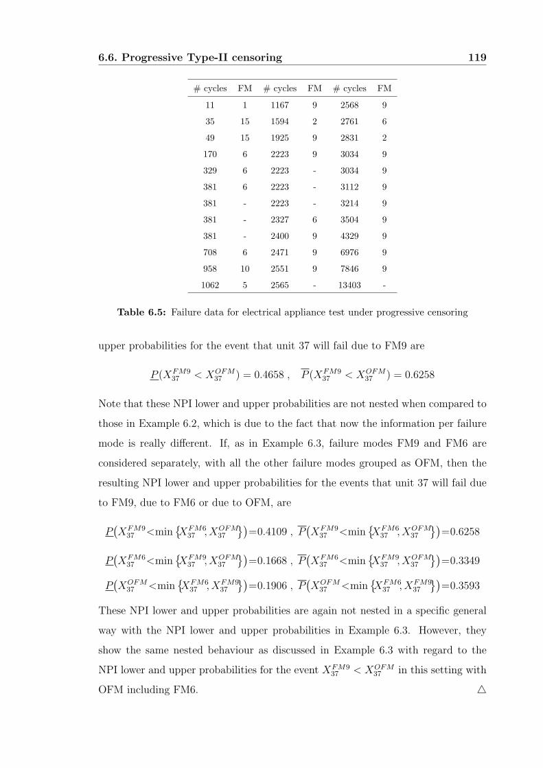
6.6. Progressive Type-II censoring 119
# cycles FM # cycles FM # cycles FM
11 1 1167 9 2568 9
35 15 1594 2 2761 6
49 15 1925 9 2831 2
170 6 2223 9 3034 9
329 6 2223 - 3034 9
381 6 2223 - 3112 9
381 - 2223 - 3214 9
381 - 2327 6 3504 9
381 - 2400 9 4329 9
708 6 2471 9 6976 9
958 10 2551 9 7846 9
1062 5 2565 - 13403 -
Table 6.5: Failure data for electrical appliance test under progressive censoring
upper probabilities for the event that unit 37 will fail due to FM9 are
P (XFM937 < XOFM
37 ) = 0.4658 , P (XFM937 < XOFM
37 ) = 0.6258
Note that these NPI lower and upper probabilities are not nested when compared to
those in Example 6.2, which is due to the fact that now the information per failure
mode is really different. If, as in Example 6.3, failure modes FM9 and FM6 are
considered separately, with all the other failure modes grouped as OFM, then the
resulting NPI lower and upper probabilities for the events that unit 37 will fail due
to FM9, due to FM6 or due to OFM, are
P(
XFM937 <min
XFM637 , XOFM
37
)
=0.4109 , P(
XFM937 <min
XFM637 , XOFM
37
)
=0.6258
P(
XFM637 <min
XFM937 , XOFM
37
)
=0.1668 , P(
XFM637 <min
XFM937 , XOFM
37
)
=0.3349
P(
XOFM37 <min
XFM637 , XFM9
37
)
=0.1906 , P(
XOFM37 <min
XFM637 , XFM9
37
)
=0.3593
These NPI lower and upper probabilities are again not nested in a specific general
way with the NPI lower and upper probabilities in Example 6.3. However, they
show the same nested behaviour as discussed in Example 6.3 with regard to the
NPI lower and upper probabilities for the event XFM937 < XOFM
37 in this setting with
OFM including FM6. 4
6.7. Concluding remarks 120
6.7 Concluding remarks
In this chapter, NPI for competing risks has been presented, with focus on the
event that the next unit will fail due to a specific failure mode. Some specific
properties and special cases are discussed and illustrated via examples in Section
6.5. As such, NPI is widely applicable and it is usually straightforward to implement
different censoring scenarios, as briefly discussed and illustrated in Section 6.6 for
a specific progressive censoring scheme. Developing NPI to take into account the
dependence between failure modes could be an interesting and challenging topic for
future research.
Chapter 7
Comparison with terminated tails
7.1 Introduction
There are many situations in statistical practice where the information available
consists of precise measurements of real-valued data only within a specific range,
with in addition the numbers of observations to the left and to the right of this range
available. This can be due to many reasons related to experimental design or some
problems with regard to data collection. For example, a lifetime experiment may be
ended before all units have failed in order to save costs and time, see Chapters 2 and
3, or very small measurements may not be available in risk analyses due to limits
of detection of the measurement method. It may also be the case that complete
data are available, but that the statistician choses to disregard the precise values
of very small or very large observations, often called ’outliers’, due to doubt about
the collection or recording of the data. A further possibility is that only a part of
the data range is considered relevant for the inference, as may occur for medical
diagnostics tests.
Coolen and Yan [27] presented the assumption rc-A(n) which is suitable for right-
censored data, see also Subsection 1.3.2. As part of the justification of rc-A(n),
Coolen and Yan [27] introduced and justified what they called the assumption A(n),
which follows from A(n) and was suitable for data with the upper tail terminated.
In Section 7.3, we will use this assumption, together with similar arguments for
lower tail termination, to derive the assumption related to A(n) that is suitable and
121
7.2. Classical methods 122
appropriate for the kind of data considered in this chapter. The assumption rc-
A(n) is suitable for data sets with multiple right-censored observations at different
time points. We do not combine terminated tails with such further right-censorings
within the non-terminated part of the data, doing so would not cause difficulties but
it adds little to the presentation of the main ideas and results in this chapter. An
obvious solution is to develop a software package (e.g. in R) to enable calculation
of the NPI lower and upper probabilities for such a scenario. The R commands for
comparing two groups, provided in the appendix of this thesis, can be used as a
starting point.
For the problem considered in this chapter, namely Nonparametric Predictive
Inference (NPI) for comparison of two groups of real-valued data with terminated
tails, we consider the two groups to be completely independent and apply the suitable
A(n) assumption per group, as the basis of our inference. We present NPI lower and
upper probabilities for the event that the value of a future observation from one
group is less than the value of a future observation from the other group.
In Section 7.2, two classical tests are briefly reviewed. The specific details of
NPI for real-valued data with terminated tails are presented in Section 7.3, followed
by the general results for pairwise comparison with such data in Section 7.4. Some
special cases are discussed in Section 7.5, and an example is provided, in Section
7.6, to illustrate the theory presented in this chapter. Some concluding remarks are
made in Section 7.7.
7.2 Classical methods
There are several robust techniques in the literature for comparing two independent
groups. In this section we briefly review two methods for such comparison, following
[37, 80] in definitions and notation. The so-called Yuen-Welch test [82] is based on
comparing the corresponding sample trimmed means of the two groups, it tests
the null hypothesis that the two groups have equal trimmed means. Suppose nx
and ny are the numbers of observations from group X and Y , respectively. Let γ
be the amount of trimming from both tails, then the remaining observations from
7.2. Classical methods 123
both groups are hx = nx − 2 bγnxc and hy = ny − 2 bγnyc, where bac is the largest
integer not greater than a. The trimmed means, calculated from these remaining
observations, are denoted by xt and yt. The Yuen-Welch test statistic is
Tγ =xt − yt√
dx + dy
where dx = (nx− 1)s2wx/hx(hx− 1) and dy = (ny − 1)s2wy
/hy(hy − 1). The quantities
s2wxand s2wy
are the Winsorized sample variances, calculated from the sample where
the trimmed observations from the left (right) tail are given the same value as
the smallest (largest) observation from the non-trimmed observations. Under the
null hypothesis, this test statistic Tγ has approximately a t-distribution with the
following degrees of freedom,
υTγ= (dx + dy)
2
(
d2xhx − 1
+d2y
hy − 1
)−1
One may want to compare the two groups by testing the null hypothesis that
P (X < Y ) = 0.5. The well known Wilcoxon-Mann-Whitney test [51] can be used
for this setting. In the case of unequal variances and with ties occurring, one may
use the modified version of the Wilcoxon-Mann-Whitney test proposed by Brunner
and Munzel [14], in which for tied observations the midranks (the average of their
ranks) are used. Let M ix (i = 1, . . . , nx) and M j
y (j = 1, . . . , ny) be the midranks of
X and Y within the pooled sample, let Mx and My be the corresponding means of
these midranks, and let V ix and V j
y be the midranks of X and Y within each sample.
Then the Brunner-Munzel test statistic is
B = (My − Mx)/(nx + ny)√
s2bx/nxn2y + s2by/n
2xny
where
s2bx=1
nx−1
nx∑
i=1
(
M ix−V i
x−Mx +nx+1
2
)2
, s2by=1
ny−1
ny∑
j=1
(
M jy−V j
y −My +ny+1
2
)2
The distribution of B is approximately a t-distribution with the following degrees
of freedom,
υB =
(
s2bxny
+s2bynx
)2(
s4bxn2y(nx − 1)
+s4by
n2x(ny − 1)
)−1
For more details and for R commands functions, which can be used in calculation,
we refer to [80].
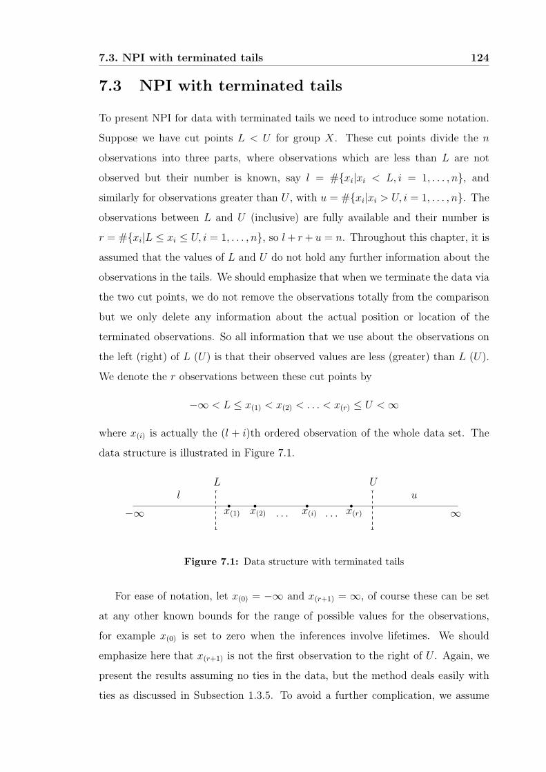
7.3. NPI with terminated tails 124
7.3 NPI with terminated tails
To present NPI for data with terminated tails we need to introduce some notation.
Suppose we have cut points L < U for group X. These cut points divide the n
observations into three parts, where observations which are less than L are not
observed but their number is known, say l = #xi|xi < L, i = 1, . . . , n, and
similarly for observations greater than U , with u = #xi|xi > U, i = 1, . . . , n. Theobservations between L and U (inclusive) are fully available and their number is
r = #xi|L ≤ xi ≤ U, i = 1, . . . , n, so l+ r+ u = n. Throughout this chapter, it is
assumed that the values of L and U do not hold any further information about the
observations in the tails. We should emphasize that when we terminate the data via
the two cut points, we do not remove the observations totally from the comparison
but we only delete any information about the actual position or location of the
terminated observations. So all information that we use about the observations on
the left (right) of L (U) is that their observed values are less (greater) than L (U).
We denote the r observations between these cut points by
−∞ < L ≤ x(1) < x(2) < . . . < x(r) ≤ U < ∞
where x(i) is actually the (l + i)th ordered observation of the whole data set. The
data structure is illustrated in Figure 7.1.
−∞r
x(1)
r
x(2) . . .r
x(i)
r
x(r). . . ∞ul
UL
Figure 7.1: Data structure with terminated tails
For ease of notation, let x(0) = −∞ and x(r+1) = ∞, of course these can be set
at any other known bounds for the range of possible values for the observations,
for example x(0) is set to zero when the inferences involve lifetimes. We should
emphasize here that x(r+1) is not the first observation to the right of U . Again, we
present the results assuming no ties in the data, but the method deals easily with
ties as discussed in Subsection 1.3.5. To avoid a further complication, we assume
7.3. NPI with terminated tails 125
throughout this chapter that there are observations in the interval [L,U ], so r > 0.
The following theorem gives an assumption directly related to A(n), and indeed
implied by A(n) taking the specific nature of the reported data into account.
Theorem 7.1 (The assumption Att(n)). The assumption Att
(n) is that the probability
distribution for a real-valued random quantity Xn+1, on the basis of the data ter-
minated at two cut points L and U as described above, is partially specified by the
following M -function values:
MXn+1(x(i), x(i+1)) =1
n+ 1, i = 0, 1, . . . , r
MXn+1(−∞, L) =l
n+ 1and MXn+1(U,∞) =
u
n+ 1.
Proof. The justification of Att(n) is similar to the justification of A(n) given by Coolen
and Yan [26], but that assumption is only for termination of the upper tail of data,
which they then build upon to enable dealing with general right-censored data.
Suppose that we actually had all n observations, and were interested in inference on
Xn+1. Then A(n) would assign probability mass 1/(n+ 1) for Xn+1 to each interval
of the partition of the real-line created by the data. With l observations left of
L, yet without any further assumptions on where these observations are, it is clear
that a probability mass of l/(n+ 1) has to be constrained to (−∞, L). In addition,
there is a probability mass 1/(n+1) between the largest observation to the left of L
and x(1), the smallest observation in the interval [L,U ]. Again, without any further
assumptions, this probability mass can only be assigned to (−∞, x(1)), or, of course,
(x(0), x(1)) if another lower limit, x(0), of the range of possible values for Xn+1 is
known. The arguments for the assignment of probability masses at the upper tail
are identical. For the intervals (x(i), x(i+1)), i = 1, . . . , r−1, which are within [L,U ],
this assignment is fully in line with the regular assumption A(n).
The cut points L and U can arise from practical aspects of the experiments or
data collection, or they can be chosen by the statistical analyst, for example to
guard against influence of outliers which may be due to measurement or recording
errors. It is crucial that they do not hold information on the observations in the
tails, apart from this there are no restrictions on how they are chosen. For example,
7.4. Comparing two groups with terminated tails 126
they could be chosen to terminate the data by a certain percentage from either a
single tail or from both tails. One could argue that any combination of cut points
together with explicitly observed values between the cut points may contain some
information about data in the tails, for example related to extreme value theory in
statistics [32], but this would always result from additional assumptions, as is always
the case with such extrapolation. In NPI, we typically try to minimize additional
assumptions, hence we make no assumptions about location of observations in the
terminated tails at all. It should be emphasized that, although by terminating the
tails of the data we are focusing on only a part of the real-line, this is only for
as far as the data are concerned. The inferences for the future observation Xn+1
are explicitly over the whole real-line (or known part of that, e.g. the non-negative
values for lifetimes).
7.4 Comparing two groups with terminated tails
Suppose that X1, . . . , Xnx, Xnx+1 are exchangeable real-valued random quantities
from group X and Y1, . . . , Yny, Yny+1 are exchangeable real-valued random quantities
from group Y , with complete independence of the two groups. We use similar
notation as in the previous section, adding an index to indicate the specific group.
Let Lx < Ux be the cut points for group X and Ly < Uy for group Y . For each
group, these cut points divide the data per group into three parts. For group X
(Y ), there are lx (ly) observations which are only known to be less than Lx (Ly),
ux (uy) which are only known to be greater than Ux (Uy), while the rx (ry) ordered
observations between the cut points are fully known and denoted by
−∞ < Lx ≤ x(1) < x(2) < . . . < x(rx) ≤ Ux < ∞
−∞ < Ly ≤ y(1) < y(2) < . . . < y(ry) ≤ Uy < ∞
Let x(0) = y(0) = −∞ and x(rx+1) = y(ry+1) = ∞.
The NPI method for comparison of groupsX and Y is explicitly in terms of future
observations Xnx+1 and Yny+1, for which we assume Att(nx)
and Att(ny)
, respectively, so
their M -function values follow from Theorem 7.1. The NPI comparison of these two
7.4. Comparing two groups with terminated tails 127
groups is based on the sharpest bounds for the probability for the event Xnx+1 <
Yny+1 that are in agreement with these M -function values, without making any
further assumptions. These bounds are lower and upper probabilities [1, 76, 79],
denoted by P = P (Xnx+1 < Yny+1) and P = P (Xnx+1 < Yny+1), respectively. These
NPI lower and upper probabilities are given in Theorem 7.2.
Theorem 7.2. Based on data with terminated tails as discussed above, the NPI
lower and upper probabilities for the event Xnx+1 < Yny+1 are
P = A
[
ry∑
j=1
lx 1Lx < y(j)+rx∑
i=1
1x(i) < y(j)
+
uy
lx 1Lx < Uy+rx∑
i=1
1x(i) < Uy
]
(7.1)
P = A
[
ry∑
j=1
ux 1Ux < y(j)+rx∑
i=1
1x(i) < y(j)
+ ly
ux 1Ux < Ly +
rx∑
i=1
1x(i) < Ly
+ (lx + 1)(ly + ry) + (uy + 1)(nx + 1)
]
(7.2)
where A = ((nx + 1)(ny + 1))−1.
Proof. The M -function values for Xnx+1 and Yny+1, based on the assumptions Att(nx)
and Att(ny)
, respectively, together with the nx (ny) observations for group X (Y ), are,
according to Theorem 7.1,
MXnx+1(x(i), x(i+1)) =1
nx + 1, i = 0, 1, . . . , rx
MXnx+1(−∞, Lx) =lx
nx + 1and MXnx+1(Ux,∞) =
ux
nx + 1
MYny+1(y(j), y(j+1)) =1
ny + 1, j = 0, 1, . . . , ry
MYny+1(−∞, Ly) =ly
ny + 1and MYny+1(Uy,∞) =
uy
ny + 1
The probability for the event Xnx+1 < Yny+1, i.e. P = P (Xnx+1 < Yny+1), can be
written as
P = P(
Xnx+1 < Yny+1, Yny+1 ∈ (−∞, Ly))
+ P(
Xnx+1 < Yny+1, Yny+1 ∈ (Uy,∞))
+
ry∑
j=0
P(
Xnx+1 < Yny+1, Yny+1 ∈ (y(j), y(j+1)))
7.4. Comparing two groups with terminated tails 128
The NPI lower probability for the event Xnx+1 < Yny+1 is obtained as follows:
P ≥ P (Xnx+1 < −∞)ly
ny + 1+
ry∑
j=0
P (Xnx+1 < y(j))1
ny + 1+ P (Xnx+1 < Uy)
uy
ny + 1
≥ A
[
ry∑
j=0
lx 1Lx < y(j)+rx∑
i=0
1x(i+1) < y(j)+ ux 1∞ < y(j)
+
uy
lx 1Lx < Uy+rx∑
i=0
1x(i+1) < Uy+ ux 1∞ < Uy]
= A
[
ry∑
j=1
lx 1Lx<y(j)+rx∑
i=1
1x(i)<y(j)
+uy
lx 1Lx<Uy+rx∑
i=1
1x(i)<Uy]
The first inequality follows by putting all probability masses for Yny+1 corresponding
to the intervals (−∞, Ly), (y(j), y(j+1)) (j = 0, . . . , ry) and (Uy,∞) to the left end
points of these intervals, and by using Lemma 1.4 for the nested intervals. The
second inequality follows by putting all probability masses for Xnx+1 corresponding
to the intervals (−∞, Lx), (x(i), x(i+1)) (i = 0, . . . , rx) and (Ux,∞) to the right end
points of these intervals. The upper probability is obtained in a similar way, but now
all M -function masses for the random quantities involved are put at the opposite
end points of the respective intervals, which leads to
P ≤ P (Xnx+1 < Ly)ly
ny + 1+
ry∑
j=0
P (Xnx+1 < y(j+1))1
ny + 1+ P (Xnx+1 < ∞)
uy
ny + 1
= P (Xnx+1 < Ly)ly
ny + 1+
ry∑
j=1
P (Xnx+1 < y(j))1
ny + 1+
uy + 1
ny + 1
≤ A
[
ly
lx 1−∞ < Ly+rx∑
i=0
1x(i) < Ly+ ux 1Ux < Ly
+
ry∑
j=1
lx 1−∞< y(j)+rx∑
i=0
1x(i)< y(j)+ ux 1Ux< y(j)
+(uy+1)(nx+1)
]
= A
[
ly
rx∑
i=1
1x(i) < Ly+ ux 1Ux < Ly
+
ry∑
j=1
rx∑
i=1
1x(i) < y(j) +
ux 1Ux < y(j)
+ (lx + 1)(ly + ry) + (uy + 1)(nx + 1)
]
It is straightforward to show that these NPI lower and upper probabilities satisfy
the conjugacy property. These NPI lower and upper probabilities are the most
7.5. Special cases 129
conservative lower and upper bounds that correspond to all possible orderings of
the data in the terminated tails. Hence, if Lx or Ly increases, or Ux or Uy decreases,
the number of data in the terminated tails can increase (it cannot decrease), which
could lead to decrease (but not increase) of the lower probability (7.1) and to increase
(but not decrease) of the upper probability (7.2).
7.5 Special cases
An advantage of presenting the general result of this chapter, in Section 7.4, is that
many important inferential problems are special cases of such comparisons with
terminated tails, hence the NPI comparison methods for such special cases follow
immediately from Theorem 7.2. In this section, we briefly discuss four special cases.
1. Equal lower and upper tails termination.
If Lx = Ly = L and Ux = Uy = U , then the NPI lower probability (7.1) and
upper probability (7.2) are
P = A
[
ry∑
j=1
rx∑
i=1
1x(i) < y(j)+ lx(ry + uy) + rxuy
]
P = A
[
ry∑
j=1
rx∑
i=1
1x(i) < y(j)+ (lx + 1)(ly + ry) + (uy + 1)(nx + 1)
]
This situation enables a straightforward analysis of the numbers of observations in
the two groups for which the exact information could be deleted by terminating
the tails, whilst still achieving P > 0.5, which might be interpreted as a strong
indication that Xnx+1 < Yny+1. Such a study can be relevant from the perspective
of robust inference, this is briefly discussed in Section 7.7. Suppose that nx = ny = n,
and that the data within the interval [L,U ] are maximally supportive for the event
Xnx+1 < Yny+1, meaning that the corresponding NPI lower and upper probabilities
P and P are maximal over all possible configurations of the data for groups X
and Y over this interval. It is easily seen and verified that this holds if all xi’s in
[L,U ] are less than all yj’s in this interval. For this situation, P > 0.5 if and only if
(n−ux)(n− ly) > 0.5(n+1)2. For example, this implies that for n = 20 observations
from each group, one could have P > 0.5 if ly = 5 and ux = 5, if the xi’s in the
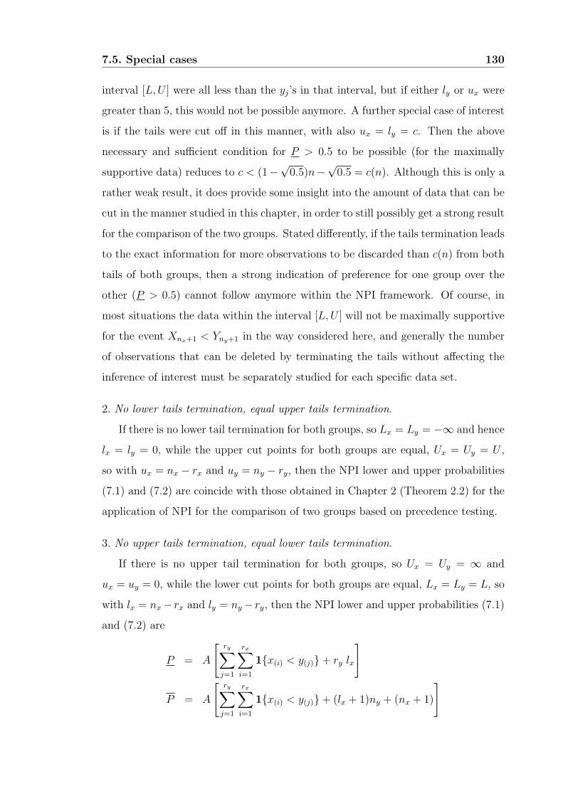
7.5. Special cases 130
interval [L,U ] were all less than the yj’s in that interval, but if either ly or ux were
greater than 5, this would not be possible anymore. A further special case of interest
is if the tails were cut off in this manner, with also ux = ly = c. Then the above
necessary and sufficient condition for P > 0.5 to be possible (for the maximally
supportive data) reduces to c < (1−√0.5)n−
√0.5 = c(n). Although this is only a
rather weak result, it does provide some insight into the amount of data that can be
cut in the manner studied in this chapter, in order to still possibly get a strong result
for the comparison of the two groups. Stated differently, if the tails termination leads
to the exact information for more observations to be discarded than c(n) from both
tails of both groups, then a strong indication of preference for one group over the
other (P > 0.5) cannot follow anymore within the NPI framework. Of course, in
most situations the data within the interval [L,U ] will not be maximally supportive
for the event Xnx+1 < Yny+1 in the way considered here, and generally the number
of observations that can be deleted by terminating the tails without affecting the
inference of interest must be separately studied for each specific data set.
2. No lower tails termination, equal upper tails termination.
If there is no lower tail termination for both groups, so Lx = Ly = −∞ and hence
lx = ly = 0, while the upper cut points for both groups are equal, Ux = Uy = U ,
so with ux = nx − rx and uy = ny − ry, then the NPI lower and upper probabilities
(7.1) and (7.2) are coincide with those obtained in Chapter 2 (Theorem 2.2) for the
application of NPI for the comparison of two groups based on precedence testing.
3. No upper tails termination, equal lower tails termination.
If there is no upper tail termination for both groups, so Ux = Uy = ∞ and
ux = uy = 0, while the lower cut points for both groups are equal, Lx = Ly = L, so
with lx = nx− rx and ly = ny − ry, then the NPI lower and upper probabilities (7.1)
and (7.2) are
P = A
[
ry∑
j=1
rx∑
i=1
1x(i) < y(j)+ ry lx
]
P = A
[
ry∑
j=1
rx∑
i=1
1x(i) < y(j)+ (lx + 1)ny + (nx + 1)
]
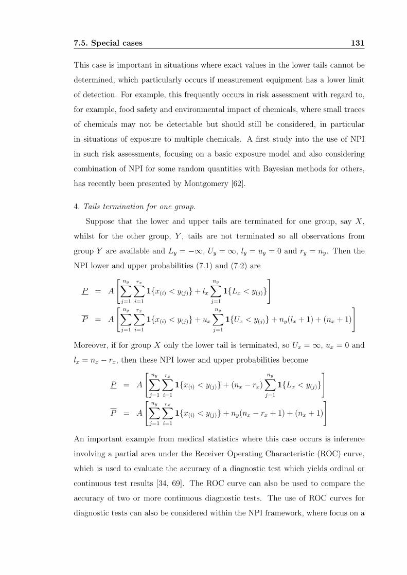
7.5. Special cases 131
This case is important in situations where exact values in the lower tails cannot be
determined, which particularly occurs if measurement equipment has a lower limit
of detection. For example, this frequently occurs in risk assessment with regard to,
for example, food safety and environmental impact of chemicals, where small traces
of chemicals may not be detectable but should still be considered, in particular
in situations of exposure to multiple chemicals. A first study into the use of NPI
in such risk assessments, focusing on a basic exposure model and also considering
combination of NPI for some random quantities with Bayesian methods for others,
has recently been presented by Montgomery [62].
4. Tails termination for one group.
Suppose that the lower and upper tails are terminated for one group, say X,
whilst for the other group, Y , tails are not terminated so all observations from
group Y are available and Ly = −∞, Uy = ∞, ly = uy = 0 and ry = ny. Then the
NPI lower and upper probabilities (7.1) and (7.2) are
P = A
[
ny∑
j=1
rx∑
i=1
1x(i) < y(j)+ lx
ny∑
j=1
1Lx < y(j)]
P = A
[
ny∑
j=1
rx∑
i=1
1x(i) < y(j)+ ux
ny∑
j=1
1Ux < y(j)+ ny(lx + 1) + (nx + 1)
]
Moreover, if for group X only the lower tail is terminated, so Ux = ∞, ux = 0 and
lx = nx − rx, then these NPI lower and upper probabilities become
P = A
[
ny∑
j=1
rx∑
i=1
1x(i) < y(j)+ (nx − rx)
ny∑
j=1
1Lx < y(j)]
P = A
[
ny∑
j=1
rx∑
i=1
1x(i) < y(j)+ ny(nx − rx + 1) + (nx + 1)
]
An important example from medical statistics where this case occurs is inference
involving a partial area under the Receiver Operating Characteristic (ROC) curve,
which is used to evaluate the accuracy of a diagnostic test which yields ordinal or
continuous test results [34, 69]. The ROC curve can also be used to compare the
accuracy of two or more continuous diagnostic tests. The use of ROC curves for
diagnostic tests can also be considered within the NPI framework, where focus on a
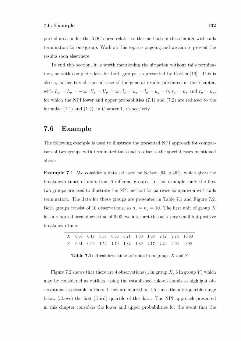
7.6. Example 132
partial area under the ROC curve relates to the methods in this chapter with tails
termination for one group. Work on this topic is ongoing and we aim to present the
results soon elsewhere.
To end this section, it is worth mentioning the situation without tails termina-
tion, so with complete data for both groups, as presented by Coolen [19]. This is
also a, rather trivial, special case of the general results presented in this chapter,
with Lx = Ly = −∞, Ux = Uy = ∞, lx = ux = ly = uy = 0, rx = nx and ry = ny,
for which the NPI lower and upper probabilities (7.1) and (7.2) are reduced to the
formulae (1.1) and (1.2), in Chapter 1, respectively.
7.6 Example
The following example is used to illustrate the presented NPI approach for compar-
ison of two groups with terminated tails and to discuss the special cases mentioned
above.
Example 7.1. We consider a data set used by Nelson [64, p.462], which gives the
breakdown times of units from 6 different groups. In this example, only the first
two groups are used to illustrate the NPI method for pairwise comparison with tails
termination. The data for these groups are presented in Table 7.1 and Figure 7.2.
Both groups consist of 10 observations, so nx = ny = 10. The first unit of group X
has a reported breakdown time of 0.00, we interpret this as a very small but positive
breakdown time.
X 0.00 0.18 0.55 0.66 0.71 1.30 1.63 2.17 2.75 10.60
Y 0.31 0.66 1.54 1.70 1.82 1.89 2.17 2.24 4.03 9.99
Table 7.1: Breakdown times of units from groups X and Y
Figure 7.2 shows that there are 4 observations (1 in groupX, 3 in group Y ) which
may be considered as outliers, using the established rule-of-thumb to highlight ob-
servations as possible outliers if they are more than 1.5 times the interquartile range
below (above) the first (third) quartile of the data. The NPI approach presented
in this chapter considers the lower and upper probabilities for the event that the
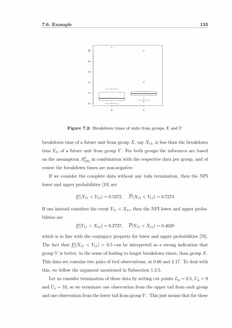
7.6. Example 133
X Y
02
46
810
Figure 7.2: Breakdown times of units from groups X and Y
breakdown time of a future unit from group X, say X11, is less than the breakdown
time Y11 of a future unit from group Y . For both groups the inferences are based
on the assumption Att(10) in combination with the respective data per group, and of
course the breakdown times are non-negative.
If we consider the complete data without any tails termination, then the NPI
lower and upper probabilities [19] are
P (X11 < Y11) = 0.5372, P (X11 < Y11) = 0.7273
If one instead considers the event Y11 < X11, then the NPI lower and upper proba-
bilities are
P (Y11 < X11) = 0.2727, P (Y11 < X11) = 0.4628
which is in line with the conjugacy property for lower and upper probabilities [76].
The fact that P (X11 < Y11) > 0.5 can be interpreted as a strong indication that
group Y is better, in the sense of leading to longer breakdown times, than group X.
This data set contains two pairs of tied observations, at 0.66 and 2.17. To deal with
this, we follow the argument mentioned in Subsection 1.3.5.
Let us consider termination of these data by setting cut points Ly = 0.5, Uy = 9
and Ux = 10, so we terminate one observation from the upper tail from each group
and one observation from the lower tail from group Y . This just means that for these
7.6. Example 134
observations the exact value is not taken into account, which might have happened
if indeed the measurements in these tails were not available, or for example if one
would have severe doubts about the accuracy of observations in these tails. The
corresponding NPI lower and upper probabilities are
P (X11 < Y11) = 0.5207, P (X11 < Y11) = 0.7355
Now suppose that we want to exclude the effect of the 4 possible outliers as
discussed above, which can for example be achieved by cut points Ly = 0.5, Uy = 4
and Ux = 10, This leads to NPI lower and upper probabilities
P (X11 < Y11) = 0.5207, P (X11 < Y11) = 0.7438
Compared to the situation discussed above with Uy = 9 and the other cut points the
same, one more observation is now terminated from the upper tail of group Y . The
effect of this is that the NPI lower probability for the event X11 < Y11 remains the
same, but the NPI upper probability increases, so the imprecision (P −P ) increases
due to more observations being terminated. Again, there is a strong indication that
group Y is better than group X.
If all units were put simultaneously on the lifetime experiment and this is ter-
minated at time 4, so Uy = Ux = 4 with no termination of the lower tails, then for
all units with observations greater than 4 the actual observations would not have
been available, instead we would only have right-censored observations at time 4 for
these units. The corresponding NPI lower and upper probabilities are
P (X11 < Y11) = 0.5372, P (X11 < Y11) = 0.7438
This lower probability exceeds 0.5, hence one may reach the same conclusion as
discussed above for the case that the experiment had not been terminated. By
terminating the experiment at time 4, 3 units have not broken down and could
possibly be used for other purposes, and, possibly more importantly, reducing the
time of the experiment may lead to cost savings. Actually, we could have ended the
experiment earlier while still getting the lower probability greater than 0.5 (and this
could not decrease by running the experiment longer), as e.g. ending the experiment
7.6. Example 135
at time 2.18, so with Uy = Ux = 2.18, would lead to 5 units not having broken down
and NPI lower and upper probabilities
P (X11 < Y11) = 0.5207, P (X11 < Y11) = 0.7603
If the experiment had been ended before time 2.17, the NPI lower probability for
the event X11 < Y11 would be less than 0.5. For example, with Uy = Ux = 2.16 the
NPI lower and upper probabilities are
P (X11 < Y11) = 0.4959, P (X11 < Y11) = 0.7769
If we terminate both tails of the data at the same cut points for both groups,
for example with Ly = Lx = 0.5 and Uy = Ux = 4, then two units would have been
terminated from the lower tail of group X and one unit from its upper tail, while
for group Y one unit would have been terminated from its lower tail and two units
from its upper tail. Then the corresponding NPI lower and upper probabilities are
P (X11 < Y11) = 0.5207, P (X11 < Y11) = 0.7438
These discussed cases illustrate that, as discussed at the end of Section 7.4,
the NPI lower (upper) probability is maximal (minimal) when all observations are
exactly included in the comparison, while deleting some of the exact information
leads to increased imprecision. This example also makes clear that varying the cut
points may have no, or only a very small effect on the actual inference. Clearly,
the lower and upper probabilities considered can only change if a change in cut
point is such that it leads to more or fewer observations in the terminated tails. For
example, for any specific cut point Ux between 2.75 and 10.60 in this example it does
not matter that the actual largest observation of group X was 10.60, the inferences
would have been the same if it were any larger value.
Before ending this example it is interesting to report some results of the classical
methods presented in Section 7.2. For the Yuen-Welch test, T0.20 = 1.67 and T0.10 =
1.24 with corresponding p-values 0.141 and 0.235, respectively, so at 5% significance
level we do not reject the null hypothesis that the trimmed means of the two groups
are equal. The same conclusion is obtained from the Brunner-Munzel test where
B = 1.21 and the p-value is 0.244. 4
7.7. Concluding remarks 136
7.7 Concluding remarks
In this chapter we have introduced NPI for comparison of two groups of real-valued
data with tails termination, which brings together a number of important applica-
tions of statistics. The main contribution of this chapter is in simultaneously dealing
with possible termination of the lower and upper tails, which was not considered
from the NPI perspective before, and which enables several important special cases
to be brought together as shown in Section 7.5. We have kept presentation relatively
basic, there are several generalizations which are important for statistical practice,
and which are relatively straightforward but which require far more complicated
notation. For example, the NPI approach presented here can quite easily be gen-
eralized to comparison of more than two groups, and it is also conceptually easy
to deal with further right-censored observations within the data by using the more
general M -functions following from rc-A(n) [27].
The problem considered in this chapter could be considered as a special case of
pairwise comparison based on interval-censored data, such that each observation is
only known to belong to an interval (which may be a single point or open-ended).
The NPI approach for this general problem is not straightforward, and provides an
exciting challenge for future research. The main problem is that the assumption
rc-A(n) does not have a straightforward generalization to deal with finite upper
bounds for the interval-censored data nor for dealing with (partially) overlapping
intervals corresponding to different observations. One could derive bounds for the
probabilities of interest by assuming that the data for one group are as large as
possible and for the other group as small as possible, and then apply the method of
Coolen [19] for such specifically assumed data, but that would lead to wide bounds
as it would neglect the exchangeability of censored data with other observations
from the same group.
There are interesting links between NPI and methods from the robust statistics
literature (see e.g. [10, 39, 43]). The NPI method for pairwise comparisons for real-
valued data presented in this chapter only takes the ranks of the non-terminated
observations into account, and as such it is insensitive to outliers even without tails
being terminated. By terminating the tails, the focus shifts explicitly to the informa-
7.7. Concluding remarks 137
tion in the non-terminated part of the data, which has some conceptual similarities
to robust statistics procedures such as trimmed means. However, our method does
not disregard the fact that there are observations in the terminated tails and it takes
the numbers of such observations into account, making such tails termination differ-
ent from truncation of the tails, which refers to situations where such numbers are
not available. As illustrated in Example 7.1, one can study how many observations
can be in the terminated tails in order to still get similar inferences, in particular
we considered the NPI lower probability for the event of interest to still exceed 0.5.
Chapter 8
Conclusions
In this thesis we have presented Nonparametric Predictive Inference (NPI) for several
comparisons problems. We introduced NPI for comparison of multiple groups of data
including right-censored observations. Different right-censoring schemes discussed
are early termination of an experiment, progressive censoring and competing risks.
Several selection events of interest are considered including selecting the best group,
the subset of best groups, and the subset including the best group. We also discussed
the situation when only a part of the data range is considered relevant for the
inference, with in addition the numbers of observations to the left and to the right
of this range available. In the appendix, we have included the R commands that have
been used for calculating NPI lower and upper probabilities for different multiple
comparison problems.
NPI is a fully nonparametric statistical approach, which explicitly does not use
any information or assumptions about the random quantities of interest other than
the relevant A(n) or rc-A(n) assumptions per group. These inferences have a frequen-
tist justification, but explicitly use the available data and do not require the use of
counterfactual data (i.e. data that could have occurred, under a specific experimen-
tal set-up, but which did not occur), which for example happens in many frequentist
methods for hypothesis testing.
Our method has the advantage that the comparison is not based on testing the
hypothesis of equality of the distributions, which, although a well established ap-
proach in classical statistics, is a somewhat surprising starting point as the reasons
138
Chapter 8. Conclusions 139
for making a comparison of different groups may make it very unlikely that ob-
servations from all groups would actually have identical distributions. In addition,
in both cases of rejection or not of such a hypothesis, it is not clear what such a
conclusion implies for the next future observation. Application of our method leads
to lower and upper probabilities for certain events of interest, which enables con-
servative decisions by basing these on the worst possible situation for the event of
interest.
A further advantage is related to the similar general advantage of statistical
methods that adhere to the likelihood principle, for which stopping rules tend not
to affect the inferences, and is a direct consequence of the fact that no hypotheses
are being tested, hence no counterfactual data play any role. Of course, one must
be happy to accept the assumptions, related to exchangeability, underlying NPI. In
addition, one does not have to restrict attention to specific censoring schemes as
presented in this thesis, as censoring can take place at any time without causing
problems for the NPI approach, as long as the censoring mechanism is independent
of the lifetime random quantities, and as long as one can reasonably assume complete
independence of the groups being compared.
As for any new statistical method, it is important to consider how it can be
applied. Of course, the assumption A(n) per group is crucial, if for example the data
or knowledge about underlying processes are such that one does not consider the
exchangeability assumption, implicit to A(n), to be appropriate, then this method
should not be applied. All classical nonparametric methods in such applications tend
to agree with this exchangeability assumption, but require additional assumptions
(e.g. similarities in the probability distribution functions corresponding to different
groups). One may well think that, in most applications, there is knowledge about the
process and groups considered that can or should be taken into account, which NPI
does not take on board. However, in all cases NPI can be considered to be a ‘base-
line method’, it provides inferences without further assumptions or information, and
this enables, for example, useful study of the outcomes of other statistical methods.
If other methods lead to conclusions which differ substantially from those following
from the NPI approach, then this will be due to the assumptions underlying the
Chapter 8. Conclusions 140
other method, which may often not have been made under complete awareness but
more for mathematical convenience. Also, it is important to be aware of the fact
that problems which appear to be identical are often formulated in substantially
different manners in different statistical methods, with each method affected by
specific features of the data. As such, we would strongly recommend the use of
several statistical methods for a problem of interest, followed by careful study of the
resulting inferences. If these all point in the same direction, then one can have great
confidence in the inferences, but if not the value of such an extensive study may
well be even greater, as detailed understanding of the different outcomes is likely to
provide more insight in the data and the actual inferential problem, as well as in
the different methods used.
The results presented in this thesis show how NPI can be applied to a variety
of problems which have been considered in the literature, mostly from classical
frequentist perspective and which are of great relevance in many applications. Most
of these problems involve multiple comparisons, and generally NPI provides exciting
opportunities for such problems via explicit focus on the next future observation per
group.
In addition to applications to a wider variety of problems, there are many re-
search challenges for the further development of NPI. These include the option to
base inferences on more than one future observation per group, which is conceptu-
ally easy although one must not forget to take account of the fact that these future
observations are inter-dependent. An interesting challenge is the requirement to
formulate appropriate predictive events of interest for a variety of inferential prob-
lems, which in this thesis was a rather straightforward comparison of the single next
observations per group. Often, however, such predictive inferences may be more
in line with intuition than established statistical methods such as hypothesis test-
ing. More generally, development of NPI for multivariate situations, including data
with covariates, is a key challenge that promises exciting research opportunities, the
results of which are strongly needed to enhance wide applicability of NPI.
Appendix A
An illustrative example of rc-A(n)
The following example is provided to illustrate the assumption rc-A(n), the full
theory is presented by Coolen and Yan [27].
First, suppose we have n = 5 observations which create 6 intervals, and all
5 observations are failure times. Then the assumption A(5) implies that the next
observation X6 will fall in any one of these intervals with probability 1/6.
Now suppose that one of these observations is right-censored at time c, so we
have 4 failure times, then A(5) cannot be used directly but we can use rc-A(5),
which is explained in detail in Figure A.1. As first step, shown in Figure A.1(a),
the probability masses for the intervals created by the 4 failure times are equal
to 1/6. There is also a probability mass 1/6 spread over the interval (c,∞) since
all we know, without making any further assumptions, that the lifetime of this
observation will be at any point beyond c (see A(n) assumption in [27, p. 32]). We
assume non-informative censoring, which means that the residual lifetime of this
censored observation is independent of the censoring process. Therefore, one can
apply A(2) but with the starting point shifted from 0 to the censoring time c, see
Figure A.1(b) (see shifted-A(n) assumption in [27, p. 33]). This gives 3 equally likely
possibilities for the actual lifetime of the censored observation, say xc, see Figures
A.1(b.1-b.3). In the case of Figure A.1(b.1), for example, this censored observation
falls somewhere between (c, x3), so the probability mass for X6 that was assigned to
the interval (x2, x3) (in Figures A.1(a-b)) would now be reassigned to the interval
(x2, xc) instead. Moreover, the probability mass that was carried forward by the
141
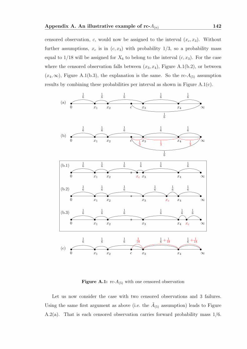
Appendix A. An illustrative example of rc-A(n) 142
censored observation, c, would now be assigned to the interval (xc, x3). Without
further assumptions, xc is in (c, x3) with probability 1/3, so a probability mass
equal to 1/18 will be assigned for X6 to belong to the interval (c, x3). For the case
where the censored observation falls between (x3, x4), Figure A.1(b.2), or between
(x4,∞), Figure A.1(b.3), the explanation is the same. So the rc-A(5) assumption
results by combining these probabilities per interval as shown in Figure A.1(c).
(a)
16
16
16
16
16
16
0 x1 x2 c x3 x4 ∞
(b)
16
16
16
16
16
16
13
13
13
0 x1 x2 c x3 x4 ∞
(b.3)16
16
16
16
16
16
0 x1 x2 xcx3 x4 ∞
(b.2)16
16
16
16
16
16
0 x1 x2 xcx3 x4 ∞
(b.1)16
16
16
16
16
16
0 x1 x2 xc x3 x4 ∞
(c)
16
16
16
16
16
118 + 1
18 + 118
0 x1 x2 c x3 x4 ∞
Figure A.1: rc-A(5) with one censored observation
Let us now consider the case with two censored observations and 3 failures.
Using the same first argument as above (i.e. the A(5) assumption) leads to Figure
A.2(a). That is each censored observation carries forward probability mass 1/6.
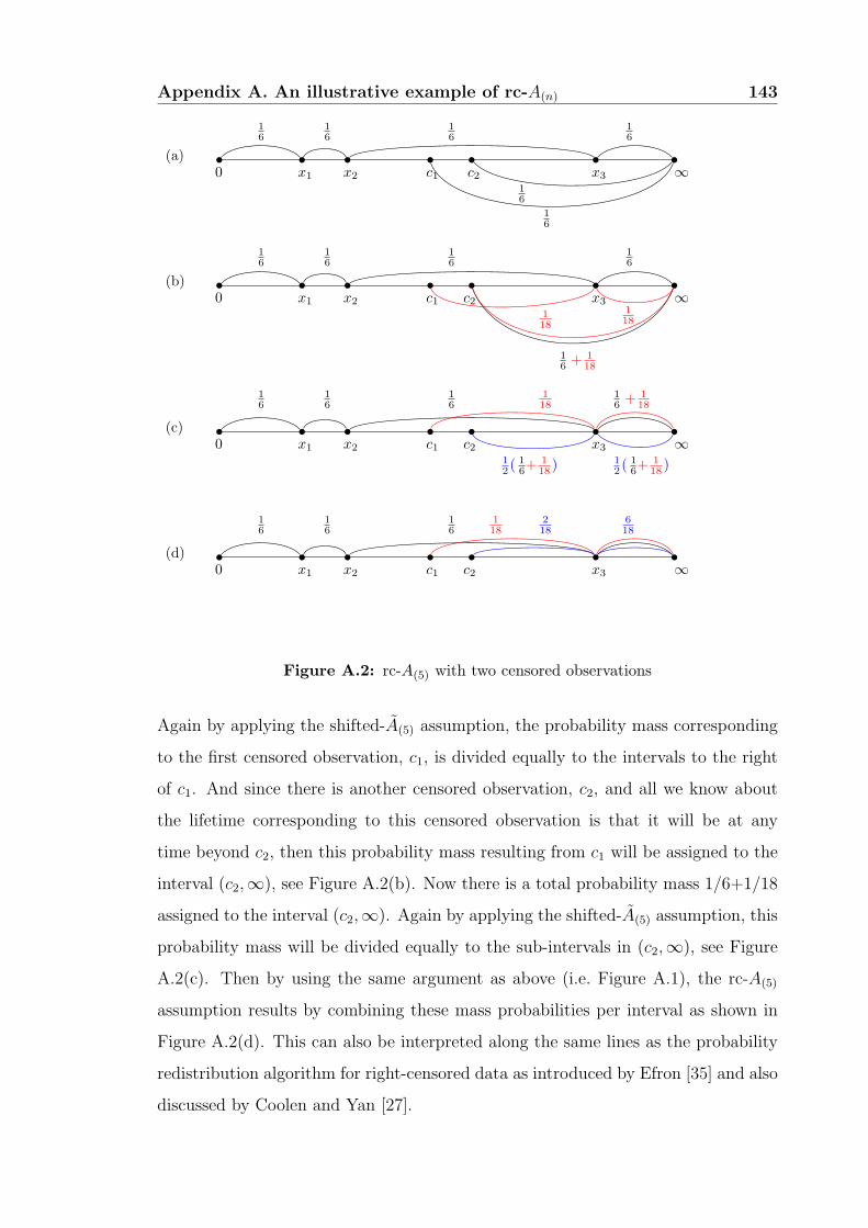
Appendix A. An illustrative example of rc-A(n) 143
(a)
16
16
16
16
16
16
0 x1 x2 c1 c2 x3 ∞
(b)
16
16
16
16
16
+ 118
118
118
0 x1 x2 c1 c2 x3 ∞
(c)
16
16
16
16
16
12 ( ) 1
2 ( )
16
+ 118 + 1
18
118 + 1
18
0 x1 x2 c1 c2 x3 ∞
(d)
16
16
16
218
618
118
0 x1 x2 c1 c2 x3 ∞
Figure A.2: rc-A(5) with two censored observations
Again by applying the shifted-A(5) assumption, the probability mass corresponding
to the first censored observation, c1, is divided equally to the intervals to the right
of c1. And since there is another censored observation, c2, and all we know about
the lifetime corresponding to this censored observation is that it will be at any
time beyond c2, then this probability mass resulting from c1 will be assigned to the
interval (c2,∞), see Figure A.2(b). Now there is a total probability mass 1/6+1/18
assigned to the interval (c2,∞). Again by applying the shifted-A(5) assumption, this
probability mass will be divided equally to the sub-intervals in (c2,∞), see Figure
A.2(c). Then by using the same argument as above (i.e. Figure A.1), the rc-A(5)
assumption results by combining these mass probabilities per interval as shown in
Figure A.2(d). This can also be interpreted along the same lines as the probability
redistribution algorithm for right-censored data as introduced by Efron [35] and also
discussed by Coolen and Yan [27].
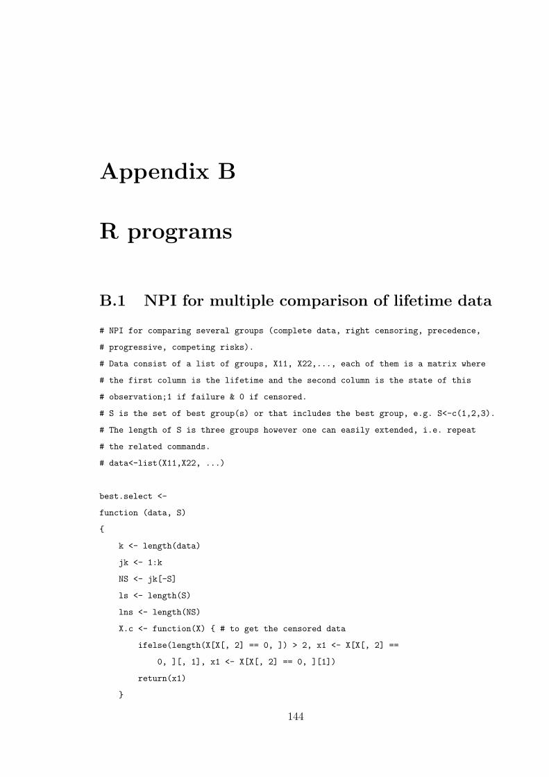
Appendix B
R programs
B.1 NPI for multiple comparison of lifetime data
# NPI for comparing several groups (complete data, right censoring, precedence,
# progressive, competing risks).
# Data consist of a list of groups, X11, X22,..., each of them is a matrix where
# the first column is the lifetime and the second column is the state of this
# observation;1 if failure & 0 if censored.
# S is the set of best group(s) or that includes the best group, e.g. S<-c(1,2,3).
# The length of S is three groups however one can easily extended, i.e. repeat
# the related commands.
# data<-list(X11,X22, ...)
best.select <-
function (data, S)
k <- length(data)
jk <- 1:k
NS <- jk[-S]
ls <- length(S)
lns <- length(NS)
X.c <- function(X) # to get the censored data
ifelse(length(X[X[, 2] == 0, ]) > 2, x1 <- X[X[, 2] ==
0, ][, 1], x1 <- X[X[, 2] == 0, ][1])
return(x1)
144
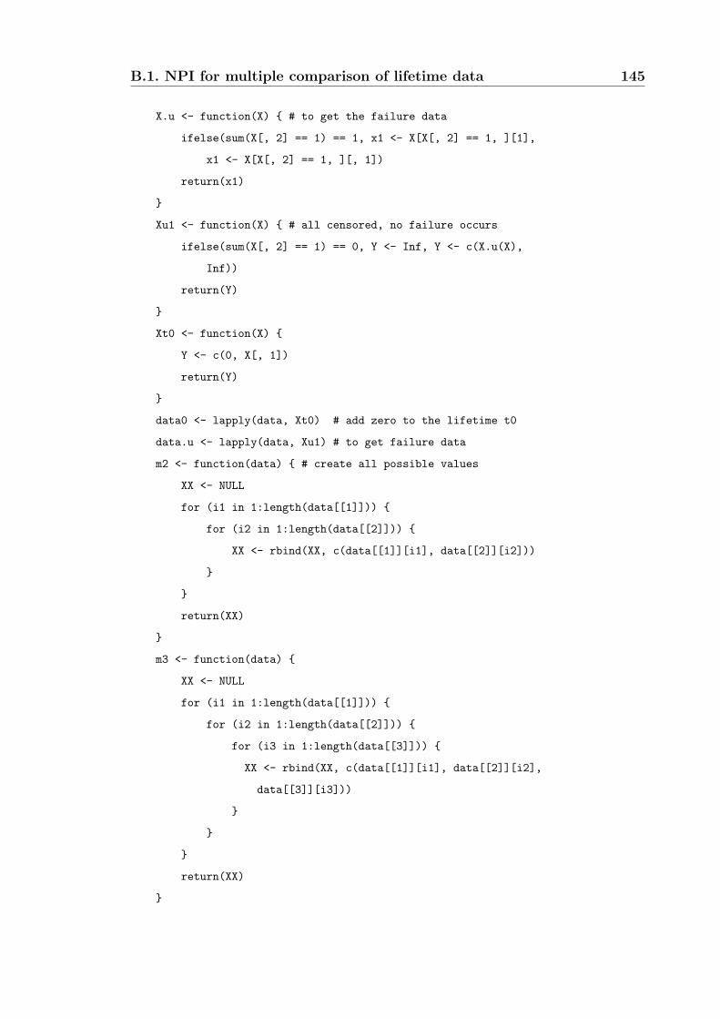
B.1. NPI for multiple comparison of lifetime data 145
X.u <- function(X) # to get the failure data
ifelse(sum(X[, 2] == 1) == 1, x1 <- X[X[, 2] == 1, ][1],
x1 <- X[X[, 2] == 1, ][, 1])
return(x1)
Xu1 <- function(X) # all censored, no failure occurs
ifelse(sum(X[, 2] == 1) == 0, Y <- Inf, Y <- c(X.u(X),
Inf))
return(Y)
Xt0 <- function(X)
Y <- c(0, X[, 1])
return(Y)
data0 <- lapply(data, Xt0) # add zero to the lifetime t0
data.u <- lapply(data, Xu1) # to get failure data
m2 <- function(data) # create all possible values
XX <- NULL
for (i1 in 1:length(data[[1]]))
for (i2 in 1:length(data[[2]]))
XX <- rbind(XX, c(data[[1]][i1], data[[2]][i2]))
return(XX)
m3 <- function(data)
XX <- NULL
for (i1 in 1:length(data[[1]]))
for (i2 in 1:length(data[[2]]))
for (i3 in 1:length(data[[3]]))
XX <- rbind(XX, c(data[[1]][i1], data[[2]][i2],
data[[3]][i3]))
return(XX)
B.1. NPI for multiple comparison of lifetime data 146
# calculate the product terms to use later for Mfun and prob
cond <- function(X, y)
P1 <- NULL
n <- nrow(X)
Xc <- X.c(X)
ncc <- function(X, cr) # calculate the term in the product term
(sum(X[, 1] >= cr) + 1)/sum(X[, 1] >= cr)
cr.obs <- Xc[Xc < y]
n.cr.obs <- length(cr.obs) # calculate the condition under the product term
ifelse(n.cr.obs == 0 | sum(X[, 2] == 0) == 0, P1 <- 1,
for (j in 1:n.cr.obs)
P1[j] <- ncc(X, cr.obs[j])
)
P3 <- prod(P1)/(n + 1)
return(P3)
# calculate Mfun and prob
Mfun <- function(X)
Y <- rbind(c(0, 1), X)
ny <- nrow(Y)
Mu <- NULL
for (i in 1:ny)
Mu[i] <- (sum(X[, 1] >= Y[, 1][i]))^(Y[, 2][i] -
1) * cond(X, Y[, 1][i])
return(Mu)
Prob <- function(X)
Y <- Xu1(X)
ny <- length(Y)
P4 <- NULL
for (i in 1:ny)
P4[i] <- cond(X, Y[i])
return(P4)
B.1. NPI for multiple comparison of lifetime data 147
# To calculate X<Y times M-function or Prob
fun1 <- function(X, Y, MP)
d <- matrix(0, length(X), length(Y))
for (i in 1:length(Y))
for (j in 1:length(X))
d[j, i] <- sum(X[j] < Y[i])
d1 <- MP %*% d
return(d1)
MM <- lapply(data, Mfun)
PP <- lapply(data, Prob)
# m=1
if (ls == 1)
XL <- unlist(data0[S])
if (ls == 1)
XU <- unlist(data.u[S])
if (ls == 1)
MMS <- unlist(MM[S])
if (ls == 1)
PPS <- unlist(PP[S])
# m=2
if (ls == 2)
XL <- m2(data0[S])
if (ls == 2)
XU <- m2(data.u[S])
if (ls == 2)
MMS <- m2(MM[S])
if (ls == 2)
PPS <- m2(PP[S])
# m=3
if (ls == 3)
XL <- m3(data0[S])
if (ls == 3)
XU <- m3(data.u[S])
if (ls == 3)

B.1. NPI for multiple comparison of lifetime data 148
MMS <- m3(MM[S])
if (ls == 3)
PPS <- m3(PP[S])
ifelse(ls == 1, prod.M <- MMS, prod.M <- apply(MMS, 1, prod))
ifelse(ls == 1, prod.P <- PPS, prod.P <- apply(PPS, 1, prod))
# compute the minmum in subset best case
ifelse(ls == 1, Min.XL <- XL, Min.XL <- apply(XL, 1, min))
ifelse(ls == 1, Min.XU <- XU, Min.XU <- apply(XU, 1, min))
# compute the maximum in subset include the best case
ifelse(ls > 1, Max.XL <- apply(XL, 1, max), Max.XL <- XL)
ifelse(ls > 1, Max.XU <- apply(XU, 1, max), Max.XU <- XU)
# Select the best groups & the subset include the best
Lprob <- function(y)
s1 <- NULL
ifelse(lns == 1, s1 <- fun1(unlist(data.u[NS]), y, unlist(PP[NS])),
for (j in 1:lns)
s1 <- rbind(s1, fun1(data.u[NS][[j]], y, PP[NS][[j]]))
)
ifelse(lns > 1, Z <- sum(apply(s1, 2, prod) * prod.M),
Z <- sum(s1 * prod.M))
return(Z)
Uprob <- function(y)
s2 <- NULL
ifelse(lns == 1, s2 <- fun1(unlist(data0[NS]), y, unlist(MM[NS])),
for (j in 1:lns)
s2 <- rbind(s2, fun1(data0[NS][[j]], y, MM[NS][[j]]))
)
ifelse(lns > 1, Z <- sum(apply(s2, 2, prod) * prod.P),
Z <- sum(s2 * prod.P))
return(Z)
print(c("Lprob.best", "Uprob.best", "Lprob.include", "Uprob.include"))
return(round(c(Lprob(Min.XL), Uprob(Min.XU), Lprob(Max.XL),
Uprob(Max.XU)), 4))
### END ###
B.2. NPI for comparing two groups with terminated tails 149
B.2 NPI for comparing two groups with termi-
nated tails
# NPI for comparing two groups, Terminated tails (Y is the best group)
ttfun <-
function (X, Y, Lx, Ux, Ly, Uy)
# Data & choose the cut points
nx <- length(X)
ny <- length(Y)
nly <- sum(Y < Ly)
nuy <- sum(Y > Uy)
nry <- sum(Y >= Ly & Y <= Uy)
nlx <- sum(X < Lx)
nux <- sum(X > Ux)
nrx <- sum(X >= Lx & X <= Ux)
Yr <- Y[Y >= Ly & Y <= Uy]
Xr <- X[X >= Lx & X <= Ux]
Mlx <- nlx/(nx + 1)
Mrx <- rep(1, nrx)/(nx + 1)
Mux <- nux/(nx + 1)
Mly <- nly/(ny + 1)
Mry <- rep(1, nry)/(ny + 1)
Muy <- nuy/(ny + 1)
fun1 <- function(X, Y, MP) # To calculate X<Y times M-function
d <- matrix(0, length(X), length(Y))
for (i in 1:length(Y))
for (j in 1:length(X))
d[j, i] <- sum(X[j] < Y[i])
d1 <- MP %*% d
return(d1)
# Lower and Upper prob. that Y is the best
YU <- c(Yr, Uy)
XL <- c(Lx, Xr)
B.2. NPI for comparing two groups with terminated tails 150
YL <- c(Ly, Yr)
XU <- c(Xr, Ux)
Lprob <- sum(fun1(XL, YU, c(Mlx, Mrx)) * c(Mry, Muy))
Uprob <- sum(fun1(XU, YL, c(Mrx, Mux)) * c(Mly, Mry)) + ((nx +
1) * (ny + 1))^(-1) * ((nlx + 1) * (nly + nry) + (nuy +
1) * (nx + 1))
return(round(c(Lprob, Uprob), 4))
### END ###
Bibliography
[1] Augustin T. and Coolen F.P.A. (2004). Nonparametric predictive inference and in-
terval probability. Journal of Statistical Planning and Inference, 124(2), 251–272.
[2] Bairamov I. and Eryilmaz S. (2006). Spacings, exceedances and concomitants in
progressive type II censoring scheme. Journal of Statistical Planning and Inference,
136(3), 527–536.
[3] Balakrishnan N. and Aggarwala R. (2000). Progressive Censoring: Theory, Methods,
and Applications. Boston: Birkha.
[4] Balakrishnan N. and Frattina R. (2000). Precedence test and maximal precedence
test. In Recent Advances in Reliability Theory: Methodology, Practice and Inference,
(Editors) N. Limnios and M. Nikulin, pp. 355–378.
[5] Balakrishnan N. and Ng H.K.T. (2006). Precedence-Type Tests and Applications.
Hoboken, N.J.: Wiley.
[6] Balakrishnan N., Ng H.K.T. and Panchapakesan S. (2006). A nonparametric proce-
dure based on early failures for selecting the best population using a test for equality.
Journal of Statistical Planning and Inference, 136(7), 2087–2111.
[7] Balakrishnan N., Tripathi R.C. and Kannan N. (2008). On the joint distribution of
placement statistics under progressive censoring and applications to precedence test.
Journal of Statistical Planning and Inference, 138(5), 1314–1324.
[8] Balakrishnan N., Tripathi R.C., Kannan N. and Ng H.K.T. (2008). Precedence-type
Test based on Progressively Censored Samples. Working Papers 0054, College of
Business, University of Texas at San Antonio.
151
BIBLIOGRAPHY 152
[9] Balakrishnan N., Tripathi R.C., Kannan N. and Ng H.K.T. (2010). Some nonpara-
metric precedence-type tests based on progressively censored samples and evaluation
of power. Journal of Statistical Planning and Inference, 140(2), 559–573.
[10] Barnett V. and Lewis T. (1994). Outliers in Statistical Data. Chichester: Wiley, 3
edition.
[11] Bechhofer R.E. (1954). A single-sample multiple decision procedure for ranking means
of normal populations with known variances. Annals of Mathematical Statistics, 25(1),
16–39.
[12] Bechhofer R.E., Santner T.J. and Goldsman D.M. (1995). Design and Analysis of
Experiments for Statistical Selection, Screening and Multiple Comparisons. New York:
Wiley.
[13] Bedford T., Alkali B. and Burnham R. (2008). Competing risks in reliability. In
Encyclopedia of Quantitative Risk Analysis and Assessment, (Editors) E.L. Melnick
and B.S. Everitt, pp. 307–312. Chichester: Wiley.
[14] Brunner E. and Munzel U. (2000). The nonparametric Behrens-Fisher problem:
Asymptotic theory and a small-sample approximation. Biometrical Journal, 42(1),
17–25.
[15] Chakraborti S. and Desu M.M. (1990). Quantile tests for comparing several treat-
ments with a control under unequal right-censoring. Biometrical Journal, 32(6),
697–706.
[16] Chakraborti S. and van der Laan P. (1997). An overview of precedence-type tests for
censored data. Biometrical Journal, 39(1), 99–116.
[17] Cohen A. and Clifford J. (1963). Progressively censored samples in life testing. Tech-
nometrics, 5(3), 327–339.
[18] Cohen A.C. (1966). Query 18: Life testing and early failure. Technometrics, 8(3),
539–545.
[19] Coolen F.P.A. (1996). Comparing two populations based on low stochastic structure
assumptions. Statistics & Probability Letters, 29(4), 297–305.
BIBLIOGRAPHY 153
[20] Coolen F.P.A. (1998). Low structure imprecise predictive inference for Bayes’ prob-
lem. Statistics & Probability Letters, 36(4), 349–357.
[21] Coolen F.P.A. (2006). On nonparametric predictive inference and objective Bayesian-
ism. Journal of Logic, Language and Information, 15(1-2), 21–47.
[22] Coolen F.P.A. and Augustin T. (2009). A nonparametric predictive alternative to the
Imprecise Dirichlet Model: the case of a known number of categories. International
Journal of Approximate Reasoning, 50(2), 217–230.
[23] Coolen F.P.A., Coolen-Schrijner P. and Yan K.J. (2002). Nonparametric predictive
inference in reliability. Reliability Engineering & System Safety, 78(2), 185–193.
[24] Coolen F.P.A. and Utkin L.V. (2008). Imprecise reliability. In Encyclopedia of Quan-
titative Risk Analysis and Assessment, (Editors) B.S. Everitt and E.L. Melnick, pp.
875–881. Chichester: Wiley.
[25] Coolen F.P.A. and van der Laan P. (2001). Imprecise predictive selection based on
low structure assumptions. Journal of Statistical Planning and Inference, 98(1-2),
259–277.
[26] Coolen F.P.A. and Yan K.J. (2003). Comparing two groups of lifetime data. In
ISIPTA’03: Proceedings of the Third International Symposium on Imprecise Proba-
bilities and their Applications, (Editors) J.M. Bernard, T. Seidenfeld and M. Zaffalon,
pp. 148–161.
[27] Coolen F.P.A. and Yan K.J. (2004). Nonparametric predictive inference with right-
censored data. Journal of Statistical Planning and Inference, 126(1), 25–54.
[28] Coolen-Schrijner P., Maturi T.A. and Coolen F.P.A. (2007). Nonparametric predictive
precedence testing for two groups. In Proceedings of the 5th Mathematical Methods
in Reliability. Glasgow, United Kingdom.
[29] Coolen-Schrijner P., Maturi T.A. and Coolen F.P.A. (2009). Nonparametric predictive
precedence testing for two groups. Journal of Statistical Theory and Practice, 3(1),
273–287. Also published in: P. Coolen-Schrijner, F.P.A. Coolen, M.C. Troffaes, T.
Augustin and S. Gupta (Eds.) (2009), Imprecision in Statistical Theory and Practice,
pp. 91-105. Greensboro (NC) USA: Grace Scientific Publishing LLC.
BIBLIOGRAPHY 154
[30] Crowder M.J. (2001). Classical Competing Risks. London: Chapman & Hall.
[31] De Finetti B. (1974). Theory of Probability: A Critical Introductory Treatment.
London: Wiley.
[32] De Haan L. and Ferreira A. (2006). Extreme Value Theory: An Introduction. New
York: Springer.
[33] Desu M.M. and Raghavarao D. (2004). Nonparametric Statistical Methods for Com-
plete and Censored Data. Boca Raton: Chapman & Hall.
[34] Dodd L.E. and Pepe M.S. (2003). Partial AUC estimation and regression. Biometrics,
59(3), 614–623.
[35] Efron B. (1967). The two sample problem with censored data. In Proceedings of the
Fifth Berkeley Symposium on Mathematical Statistics and Probability, volume 4, pp.
831–853. New York: Prentice-Hall.
[36] Epstein B. (1955). Comparison of some non-parametric tests against normal al-
ternatives with an application to life testing. Journal of the American Statistical
Association, 50(271), 894–900.
[37] Fagerland M.W. and Sandvik L. (2009). Performance of five two-sample location
tests for skewed distributions with unequal variances. Contemporary Clinical Trials,
30(5), 490–496.
[38] Gupta S.S. (1965). On some multiple decision (selection and ranking) rules. Techno-
metrics, 7(2), 225–245.
[39] Hampel F.R., Ronchetti E.M., Rousseeuw P.J. and Stahel W.A. (1986). Robust Statis-
tics. New York: Wiley.
[40] Hill B.M. (1968). Posterior distribution of percentiles: Bayes’ theorem for sampling
from a population. Journal of the American Statistical Association, 63(322), 677–691.
[41] Hill B.M. (1988). De Finetti’s theorem, induction, and An, or Bayesian nonparamet-
ric predictive inference (with discussion). In Bayesian Statistics 3, (Editors) J.M.
Bernando, M.H. DeGroot, D.V. Lindley and A. Smith, pp. 211–241. Oxford Univer-
sity Press.
BIBLIOGRAPHY 155
[42] Hill B.M. (1993). Parametric models for An: Splitting processes and mixtures. Jour-
nal of the Royal Statistical Society. Series B (Methodological), 55(2), 423–433.
[43] Huber P.J. (1981). Robust Statistics. New York: Wiley.
[44] Kaplan E.L. and Meier P. (1958). Nonparametric estimation from incomplete obser-
vations. Journal of the American Statistical Association, 53(282), 457–481.
[45] Kochar S.C., Lam K.F. and Yip P.S.F. (2002). Generalized supremum tests for the
equality of cause specific hazard rates. Lifetime Data Analysis, 8(3), 277–288.
[46] Kundu D. and Joarder A. (2006). Analysis of Type-II progressively hybrid censored
data. Computational Statistics & Data Analysis, 50(10), 2509 – 2528.
[47] Kundu D., Kannan N. and Balakrishnan N. (2004). Analysis of progressively censored
competing risks data. In Handbook of Statistics 23: Advances in Survival Analysis,
(Editors) N. Balakrishnan and C.R. Rao, pp. 331–348. Amsterdam: Elsevier.
[48] Lawless J.F. (2003). Statistical Models and Methods for Lifetime Data. Hoboken,
N.J.: Wiley.
[49] Lee E.T. and Desu M.M. (1972). A computer program for comparing K samples with
right-censored data. Computer Programs in Biomedicine, 2(4), 315–321.
[50] Lehmann E.L. (1975). Nonparametrics: Statistical Methods Based on Ranks. San
Francisco: Holden-Day.
[51] Mann H.B. and Whitney D.R. (1947). On a test of whether one of two random vari-
ables is stochastically larger than the other. The Annals of Mathematical Statistics,
18(1), 50–60.
[52] Maturi T.A., Coolen-Schrijner P. and Coolen F.P.A. (2008). Early termination of
experiments in nonparametric predictive comparisons. In Proceedings International
Workshop on Applied Probability. Compiegne, France.
[53] Maturi T.A., Coolen-Schrijner P. and Coolen F.P.A. (2008). Lifetime comparisons
with early termination of experiments. In Proceedings International Seminar on Non-
parametric Inference, (Editors) J.C. Pardo-Fernandez and J. de Una-Alvarez, pp.
127–130. Vigo, Spain.
BIBLIOGRAPHY 156
[54] Maturi T.A., Coolen-Schrijner P. and Coolen F.P.A. (2009). Nonparametric predic-
tive multiple comparisons with censored data and competing risks. In ISIPTA’09:
Proceedings 6th International Symposium on Imprecise Probability: Theories and Ap-
plications, pp. 307–316. Durham, United Kingdom.
[55] Maturi T.A., Coolen-Schrijner P. and Coolen F.P.A. (2009). Nonparametric predictive
pairwise comparison for real-valued data with terminated tails. International Journal
of Approximate Reasoning, 51(1), 141–150.
[56] Maturi T.A., Coolen-Schrijner P. and Coolen F.P.A. (2009). On nonparametric pre-
dictive inference for competing risks. In Proceedings of the 18th Advances in Risk and
Reliability Technology Symposium, (Editor) L. Bartlett, pp. 196–211. Loughborough,
United Kingdom.
[57] Maturi T.A., Coolen-Schrijner P. and Coolen F.P.A. (2010). Nonparametric predic-
tive comparison of lifetime data under progressive censoring. Journal of Statistical
Planning and Inference, 140(2), 515–525.
[58] Maturi T.A., Coolen-Schrijner P. and Coolen F.P.A. (2010). Nonparametric predictive
comparison of lifetime data with early termination of experiments. In submission.
[59] Maturi T.A., Coolen-Schrijner P. and Coolen F.P.A. (2010). Nonparametric predictive
inference for competing risks. Journal of Risk and Reliability, 224(1), 11–26.
[60] Maturi T.A., Coolen-Schrijner P. and Coolen F.P.A. (2010). Nonparametric predictive
selection with early experiment termination. In submission.
[61] Montanari G.C. and Cacciari M. (1988). Progressively-censored aging tests on xlpe-
insulated cable models. IEEE Transactions on Electrical Insulation, 23(3), 365–372.
[62] Montgomery V. (2009). New Statistical Methods in Risk Assessment by Probability
Bounds. Ph.D. thesis, Durham University, Durham, UK. Available from www.npi-
statistics.com.
[63] Nelson L.S. (1963). Tables for a precedence life test. Technometrics, 5(4), 491–499.
[64] Nelson W. (1982). Applied Life Data Analysis. New York: Wiley.
BIBLIOGRAPHY 157
[65] Nelson W.B. (1972). Graphical analysis of accelerated life test data with the inverse
power law model. IEEE Transactions on Reliability, 21, 2–11.
[66] Ng H.K.T. and Balakrishnan N. (2004). Wilcoxon-type rank-sum precedence tests.
Australia and New Zealand Journal of Statistics, 46, 631–648.
[67] Ng H.K.T. and Balakrishnan N. (2005). Weighted precedence and maximal prece-
dence tests and an extension to progressive censoring. Journal of Statistical Planning
and Inference, 135(1), 197–221.
[68] Ng H.K.T., Balakrishnan N. and Panchapakesan S. (2007). Selecting the best pop-
ulation using a test for equality based on minimal Wilcoxon rank-sum precedence
statistic. Methodology and Computing in Applied Probability, 9(2), 263–305.
[69] Pepe M.S. (2003). The Statistical Evaluation of Medical Tests for Classification and
Prediction. Oxford: Oxford University Press.
[70] Pintilie M. (2006). Competing Risks: A Practical Perspective. Chichester: Wiley.
[71] Ray M.R. (2008). Competing risks. In Encyclopedia of Quantitative Risk Analysis
and Assessment, (Editors) E.L. Melnick and B.S. Everitt, pp. 301–307. Chichester:
Wiley.
[72] Shafer G. (1976). A Mathematical Theory of Evidence. Princeton (US): Princeton
University Press.
[73] Tsiatis A. (1975). A nonidentifiability aspect of the problem of competing risks. In
Proceedings of the National Academy of Sciences of the United States of America, 72,
pp. 20–22.
[74] Utkin L.V. and Coolen F.P.A. (2007). Imprecise reliability: An introductory overview.
In Computational Intelligence in Reliability Engineering, Volume 2: New Metaheuris-
tics, Neural and Fuzzy Techniques in Reliability, (Editor) G. Levitin, pp. 261–306.
New York: Springer.
[75] Verheijen J.H.M., Coolen F.P.A. and van der Laan P. (1997). Combining two clas-
sical approaches for statistical selection. Communications in Statistics: Theory and
Methods, 26(6), 1291–1312.
BIBLIOGRAPHY 158
[76] Walley P. (1991). Statistical Reasoning with Imprecise Probabilities. London: Chap-
man & Hall.
[77] Walley P. (1996). Measures of uncertainty in expert systems. Artificial Intelligence,
83(1), 1 – 58.
[78] Weichselberger K. (2000). The theory of interval-probability as a unifying concept
for uncertainty. International Journal of Approximate Reasoning, 24(2-3), 149–170.
[79] Weichselberger K. (2001). Elementare Grundbegriffe einer allgemeineren Wahrschein-
lichkeitsrechnung I. Intervallwahrscheinlichkeit als umfassendes Konzept. Heidelberg:
Physika.
[80] Wilcox R.R. (2005). Introduction to Robust Estimation and Hypothesis Testing. San
Diego, CA: Academic Press, 2 edition.
[81] Yan K.J. (2002). Nonparametric Predictive Inference with Right-Censored Data.
Ph.D. thesis, Durham University, Durham, UK. Available from www.npi-
statistics.com.
[82] Yuen K.K. (1974). The two-sample trimmed t for unequal population variances.
Biometrika, 61(1), 165–170.