nonparametric quantile regression estimation with mixed

This is a repository copy of Nonparametric Quantile Regression Estimation with Mixed Discrete and Continuous Data.

White Rose Research Online URL for this paper:https://eprints.whiterose.ac.uk/157191/

Version: Accepted Version

Article:

Li, Degui orcid.org/0000-0001-6802-308X, Li, Qi and Li, Zheng (2021) Nonparametric Quantile Regression Estimation with Mixed Discrete and Continuous Data. Journal of Business and Economic Statistics. 741–756. ISSN 0735-0015

https://doi.org/10.1080/07350015.2020.1730856

[email protected]://eprints.whiterose.ac.uk/

Reuse

Items deposited in White Rose Research Online are protected by copyright, with all rights reserved unless indicated otherwise. They may be downloaded and/or printed for private study, or other acts as permitted by national copyright laws. The publisher or other rights holders may allow further reproduction and re-use of the full text version. This is indicated by the licence information on the White Rose Research Online record for the item.

Takedown

If you consider content in White Rose Research Online to be in breach of UK law, please notify us by emailing [email protected] including the URL of the record and the reason for the withdrawal request.

Nonparametric Quantile Regression Estimation with

Mixed Discrete and Continuous Data

Degui Li∗

University of York

Qi Li†

Texas A&M University

Zheng Li‡

North Carolina State University

February 3, 2020

Abstract

In this paper, we investigate the problem of nonparametrically estimating a conditional

quantile function with mixed discrete and continuous covariates. A local linear smoothing

technique combining both continuous and discrete kernel functions is introduced to estimate the

conditional quantile function. We propose using a fully data-driven cross-validation approach

to choose the bandwidths, and further derive the asymptotic optimality theory. In addition, we

also establish the asymptotic distribution and uniform consistency (with convergence rates) for

the local linear conditional quantile estimators with the data-dependent optimal bandwidths.

Simulations show that the proposed approach compares well with some existing methods.

Finally, an empirical application with the data taken from the IMDb website is presented to

analyze the relationship between box office revenues and online rating scores.

Keywords: Bandwidth selection, Discrete regressors, Local linear smoothing, Nonparametric

estimation, Quantile regression

JEL Classification: C13, C14, C35

∗Department of Mathematics, University of York, York, YO10 5DD, UK. Email: [email protected].†The corresponding author. Department of Economics, Texas A&M University, College Station, TX, 77843, USA.

Email: [email protected].‡Department of Agricultural and Resource Economics, North Carolina State University, Raleigh, NC, 27695, USA.

Email: [email protected].

1 Introduction

In recent years, there has been an increasing interest on nonparametric estimation of the regression

models, as the nonparametric approach allows the data “speak for themselves” and thus has the

ability to detect regression structures which may be difficult to uncover by traditional parametric

modelling approaches. Various nonparametric methods have attracted much attention of statisti-

cians and econometricians (c.f., Green and Silverman, 1994; Wand and Jones, 1995; Fan and Gijbels,

1996; Pagan and Ullah, 1999; Horowitz, 2009). One of the most commonly-used nonparametric

estimation methods is the local linear smoothing method as it has advantages over the traditional

Nadaraya-Watson kernel approach, such as higher asymptotic efficiency, design adaption and

automatic boundary correction. We refer to the book by Fan and Gijbels (1996) for a detailed

account on this subject.

Most of the aforementioned literature focuses on the nonparametric estimation with continuous

regressors. However, in practice, it is not uncommon that some of the regressors might be discrete

(e.g., gender, race and religious belief). Although in principle one can split the whole sample into

many cells (determined by values of the discrete regressors) to handle the discrete variables, in

practice such a sample-splitting method quickly becomes infeasible when the number of discrete

cells is large. Indeed as pointed out by Li and Racine (2004), the naive splitting method may

perform poorly when the number of subgroups is relatively large and the number of observations

in some subgroups is small. To address this problem, they consider a nonparametric kernel-based

method which smoothes both continuous and discrete covariates. Such a method works well in

practice.

It is well known that the conditional mean function may not be a good representative of the

impact of the explanatory variables on the response variable. Hence, it is often of interest to model

conditional quantiles when studying the regression relationship between a response variable and

some explanatory variables. Since the seminal paper by Koenker and Bassett (1978), the quantile

regression method has been widely used in many disciplines such as economics, finance, political

science and other social science fields. The quantile regression serves as a robust alternative to

the mean regression. Recent developments on parametric and nonparametric quantile estimation

and inference include Yu and Jones (1998), Cai (2002), Yu and Lu (2004), Koenker and Xiao (2006),

Cai and Xu (2008), Hallin, Lu and Yu (2009), Escanciano and Velasco (2010), Kong, Linton and Xia

(2010), Belloni and Chernozhukov (2011), Galvao (2011), Guerre and Sabbah (2012), Cai and Xiao

(2012), Galvao, Lamarche and Lima (2013), Li, Lin and Racine (2013), Spokoiny, Wang and Hardle

(2013), Escanciano and Goh (2014), Qu and Yoon (2015), Racine and Li (2017), Belloni et al (2019)

and Zhu et al (2019). Koenker (2005) and Koenker et al (2017) give a comprehensive overview on

various methodologies in quantile regression and their applications. In particular, the paper by

1

Li, Lin and Racine (2013) is among the first to estimate the conditional cumulative distribution

function (CDF) nonparametrically by smoothing both the discrete and continuous covariates, and

then obtain quantile regression function estimation by inverting the estimated conditional CDF

at the desired quantiles. The bandwidths are chosen optimally in estimating the nonparametric

CDF, and therefore, they may not be optimal for estimating for estimating the conditional quantile

regression function.

In this paper, we propose a different nonparametric method to estimate the conditional quantile

function via minimizing a local linear weighted “check function” (objective function) defined in

Section 2. To tackle a general setting with mixed continuous and discrete regressors, we construct

the local linear smoothing check function with both the continuous and discrete kernel functions

involved. As the numerical performance of the local linear estimation is sensitive to the bandwidths

or smoothing parameters, we further study the choice of smoothing parameters in the local linear

quantile estimation, proposing a completely data-driven rescaled cross-validation (RCV) approach

to directly choose the optimal smoothing parameters and deriving their asymptotic optimality

property. As pointed out by Yao and Tong (1998), the RCV method is computationally faster than

the conventional “leave-one-out” cross-validation method in selecting the optimal smoothing

parameters. This advantage would be more significant in nonparametric quantile regression

estimation which lacks a closed-form solution in the estimation procedure.

The check function based quantile regression estimation method proposed in this paper has at

least three advantages over the inverse-CDF approach proposed by Li, Lin and Racine (2013). First,

it is computationally much more efficient than the inverse-CDF approach. Our check-function-

based RCV method requires O(n2) computations, whereas the inverse-CDF-based CV method

involves O(n3) computations, where n is the sample size. This is a significant improvement in the

computational aspect. The second advantage of using our method is that, besides the estimated

conditional quantile function, we also obtain the derivative function (of the conditional quantile

function with respect to the continuous components) estimate and its asymptotic theory, while

it seems difficult to obtain derivative function estimation and to derive the related asymptotic

theory if one uses the inverse-CDF method. The third advantage is that, in practice the optimal

smoothing parameters often vary over τ, and our method addresses this issue well by providing

optimal smoothing parameters for each specific quantile τ ∈ (0, 1). In contrast, the inverse-

CDF method gives the same smoothing parameters for all τ ∈ (0, 1), and does not have the

flexibility of choosing τ-dependent optimal smoothing parameters to conditional quantile function

estimation. Under some mild conditions, we prove the point-wise asymptotic normal distribution

and uniform convergence rates for the developed local linear quantile estimators using the data-

dependent bandwidths determined by the RCV approach. We use simulations to illustrate the

finite-sample behavior of the proposed method and compare our approach with some existing

2

methods. Finally we apply the proposed nonparametric quantile regression estimation method

to study the relationship between box office revenues and online rating scores using the dataset

collected from the IMDb website.

2 Local linear quantile regression estimation

Suppose that (Yi,Xi,Zi), i = 1, · · · ,n, are the observations independently drawn from an identical

distribution, where Yi ∈ R is univariate, Xi ∈ Dx is a p-dimensional continuous random vector and

Zi ∈ Dz is a q-dimensional discrete random vector, Dx ={(x1, · · · , xp)

⊺

: cj 6 xj 6 cj, j = 1, · · · ,p}

is a bounded subset of Rp with cj < cj, j = 1, · · · ,p, being bounded constants, and Dz is a finite

support of the discrete vector Zi. For expositional simplicity, we assume that each component of

Zi only takes non-negative integer values. We estimate the conditional quantile function and its

derivatives (with respect to the continuous components) by minimizing a local linear weighted

objective function, and then introduce a completely data-driven method to choose appropriate

smoothing parameters involved.

For y ∈ R, x = (x1, · · · , xp)⊺ ∈ Dx and z = (z1, · · · , zq)

⊺ ∈ Dz, we denote F(y|x, z) as the

conditional CDF of the response variable Yi (evaluated at y) given the covariates Xi = x and Zi = z.

For 0 < τ < 1, we let Qτ(x, z) be the conditional τ-quantile regression function of Yi given Xi = x

and Zi = z, i.e., Qτ(x, z) = inf {y ∈ R : F(y|x, z) > τ}, or equivalently

Qτ(x, z) = arg mina∈R

E[ρτ(Yi − a)

∣∣Xi = x,Zi = z]

, (2.1)

where ρτ(·) is the τ-quantile check function (or loss function) defined as ρτ(y) = y (τ− I{y < 0})

with I{A} being the indicator function of the set A.

We apply the local linear smoothing approach to estimate the τ-quantile regression function

Qτ(x0, z0) based on the definition given in (2.1), where x0 = (x0,1, · · · , x0,p)⊺ ∈ Dx and z0 =

(z0,1, · · · , z0,q)⊺ ∈ Dz. Due to mixture of discrete and continuous data in the regressors, two types

of kernel-weights are required to construct the locally weighted loss function. For the continuous

regressors, we use a conventional kernel weight Kh(Xi − x0) defined by

Kh(Xi − x0) =1

h1 · · ·hp

K

(Xi − x0

h

)=

p∏

j=1

1

hj

K

(Xi,j − x0,j

hj

),

where h = (h1, · · · ,hp)⊺

, hj is the bandwidth for the j-th continuous covariate Xi,j, and K(·) is a

univariate kernel function. For the discrete covariates, we use the following discrete kernel (with

3

the convention that 00 equals to 1):

Λλ(Zi, z0) =

q∏

j=1

λI{Zi,j 6=z0,j}

j ,

where λ = (λ1, · · · , λq)⊺

, λj ∈ [0, 1] is the bandwidth for the j-th discrete covariate Zi,j. The local

linear estimates of Qτ(x0, z0) and its derivatives (with respect to the continuous components)

Q′τ,j(x0, z0), j = 1, 2, · · · ,p, are obtained by minimizing the weighted loss function

Ln(α,β; x0, z0) =1

n

n∑

i=1

ρτ

(Yi − α− (Xi − x0)

⊺

β)

Kh(Xi − x0)Λλ(Zi, z0) (2.2)

with respect to α and β = (β1, · · · ,βp)⊺

. We denote the minimizers by

α ≡ Qτ(x0, z0), βj ≡ Q′τ,j(x0, z0), j = 1, · · · ,p.

The above check function based local linear conditional quantile estimator with mixed discrete

and continuous covariates was previously considered in Li and Racine (2008). However, they

did not provide asymptotic analysis on the selection of optimal smoothing parameters by some

data-driven methods, which is the main task of the present paper.

When the smoothing parameter in the discrete kernel is chosen as a vector of zeros, the above

approach reduces to the traditional local linear quantile estimation method which splits the full

sample into several groups (sub-samples) according to different values that the discrete covariates

can assume. Then one may directly apply the local linear quantile estimation methodology and

theory developed in the literature for the case of purely continuous regressors (c.f., Yu and Jones,

1998; Cai and Xu, 2008). However, as pointed out by Li and Racine (2004), such a naive sample-

splitting method may increase the estimation variance. In particular, it is well known that if the

sample size in the subgroup is too small, one cannot expect to get reliable estimation results with

the sample-splitting local linear quantile estimation method.

It is of crucial importance to appropriately select smoothing parameters in the nonparametric

local linear smoothing procedure. In this paper we propose to use a completely data-driven

method to choose the optimal bandwidth vectors h and λ. The cross-validatory bandwidth

selection criterion has been extensively studied in the context of local kernel-based mean regression

estimation with continuous regressors (c.f., Rice, 1984; Hall, Lahiri and Polzehl, 1995; Xia and Li,

2002; Leung, 2005). In recent years, there has also been an increasing interest in extending this

bandwidth selection approach to the case with mixed continuous and discrete regressors (c.f., Li

and Racine, 2004). However, most of the existing literature focuses on the bandwidth selection

4

in the kernel-based estimation in the context of conditional mean regression. Extension of the

cross-validation bandwidth selection method to the conditional quantile regression is non-trivial

and the derivation of the asymptotic optimality property is challenging as there is no closed-form

expression for the local linear quantile estimator. Li, Lin and Racine (2013) studied the bandwidth

selection in nonparametric quantile regression estimation. Their optimal bandwidths for both the

continuous and discrete regressors are chosen when estimating the nonparametric CDF. As a result,

the chosen bandwidths are optimal for the CDF estimation, but not for the quantile regression

estimation. In this paper, we introduce a data-driven method to directly select bandwidth vectors

which are optimal for quantile regression estimation.

We split the full sample into two sets: the training set M1 = {(Yi,Xi,Zi), i = 1, · · · ,m}, and

the validation set M2 = {(Yi,Xi,Zi), i = m+ 1, · · · ,n}, where m has the same order as n (say

m = ⌊n/2⌋). For j = m + 1, · · · ,n, let QM1(Xj,Zj;h, λ) ≡ Qτ,M1

(Xj,Zj;h, λ) be the local linear

estimated value of Qτ(Xj,Zj) with bandwidth vectors h and λ, which are obtained by minimizing

(2.2) with (x0, z0) and∑n

i=1 replaced by (Xj,Zj) and∑m

i=1, respectively. Define the following

objective function:

CV(h, λ) =1

n−m

n∑

j=m+1

ρτ

(Yj − QM1

(Xj,Zj;h, λ))M(Xj), (2.3)

where M(·) is a weight function that trims out observations whose continuous components are

close to the boundary. Let (hm, λm

)= arg min

(h,λ)∈Hm

CV(h, λ), (2.4)

where Hm is a set of grid points [h(k), λ(k)], k = 1, · · · ,Lm, satisfying Assumption 5(i)(ii) in

Appendix A and that

max16k6Lm

minj 6=k

‖h(k) − h(j)‖+ max16k6Lm

minj 6=k

‖λ(k) − λ(j)‖ 6 γm, (2.5)

‖ · ‖ denotes the Euclidean norm. Assumption 5(iii) in Appendix A gives some restrictions on Lm

and γm, ensuring that the grid points are sufficiently dense in the set Hm. With hm and λm, we do

the re-scaling to obtain the RCV bandwidth vectors for the full sample as

h =(h1, · · · , hp

)⊺

= hm

(mn

)1/(4+p)

and λ =(λ1, · · · , λq

)⊺

= λm

(mn

)2/(4+p)

. (2.6)

The motivation for constructing the RCV optimal bandwidth vectors (for full sample) in (2.6) is

relevant to asymptotic order of the theoretically optimal bandwidths, which will be made clear later

in the section. As the training set size in the RCV bandwidth selection is usually smaller than the

5

size n− 1 in the conventional “leave-one-out” cross-validation, we expect that the computational

time for the RCV method would be faster in particular when the full sample size is large. The

RCV method was studied by Yao and Tong (1998) for bandwidth selection in kernel regression

estimation with univariate continuous regressor, and a similar idea was recently used by Fan, Guo

and Hao (2012) and Chen, Fan and Li (2018) for error variance estimation in high-dimensional

mean regression models.

To derive the asymptotic optimality for the RCV selected bandwidths h and λ, we need some

additional notation. Let ei = Yi − Qτ(Xi,Zi) and assume that P(ei 6 0|Xi = x,Zi = z) = τ for

x ∈ Dx and z ∈ Dz. Define fxz(·, ·) as the joint probability density function of Xi and Zi and fe(·|x, z)

as the conditional density function of ei given Xi = x and Zi = z. Let Q′′τ,j(x, z), j = 1, 2, · · · ,p,

be the second-order derivative function of Qτ(·, ·) with respect to the j-th continuous component

evaluated at the point (x, z). Define

bm(Xi,Zi;h, λ) =µ2

2

p∑

j=1

h2jQ

′′τ,j(Xi,Zi) +

∑

z∈Dz

q∑

j=1

Ij(z,Zi)λj

f(Xi, z)

f(Xi,Zi)[Qτ(Xi, z) − Qτ(Xi,Zi)] ,

σ2m(Xi,Zi;h) =

1

mH· τ(1 − τ)νp

0

[fe(0|Xi,Zi)]2fxz(Xi,Zi)

,

where µj =∫ujK(u)du and νj =

∫ujK2(u)du for j = 0, 1, 2, · · · , f(x, z) = fe(0|x, z)fxz(x, z),

Ij (z, z) = I{zj 6= zj}∏q

k=1, 6=j I{zk = zk} for z = (z1, · · · , zq)⊺

and z = (z1, · · · , zq)⊺

, and H =∏p

j=1 hj.

The following theorem gives the uniform asymptotic expansion of CV(h, λ), which is crucial to

derive the asymptotic optimality of h and λ defined in (2.6).

THEOREM 2.1. Suppose that Assumptions 1–5 in Appendix A are satisfied and there exists a

constant 0 < < 1 such that m/n → . Then, we have that, uniformly over (h, λ) ∈ Hm

CV(h, λ) = CV∗ +1

2E{[b2m(Xi,Zi;h, λ) + σ2

m(Xi,Zi;h)]M(Xi)fe(0|Xi,Zi)

}+ s.o., (2.7)

where CV∗ = (n−m)−1∑n

i=m+1 ρτ(ei)M(Xi) is unrelated to h and λ, and “s.o.” represents terms

with smaller asymptotic probability orders than the second term on the right hand side of (2.7).

The proof of Theorem 2.1 is provided in Appendix B.1. Define the following mean squared

errors of the local linear quantile regression estimation for the validation set M2:

MSEM2(h, λ) =

1

n−m

n∑

i=m+1

[Qτ(Xi,Zi) − QM1

(Xi,Zi;h, λ)]2

M(Xi)fe(0|Xi,Zi), (2.8)

6

and its asymptotic leading term:

MSELM2

(h, λ) = E{[

b2m(Xi,Zi;h, λ) + σ2


}. (2.9)

Let a = (a1, · · · ,ap)⊺

and d = (d1, · · · ,dq)⊺

with aj = hj ·m1/(4+p) and dj = λj ·m2/(4+p). Then

(2.9) can be written as MSELM2

(h, λ) = m−4/(4+p)g(a,d), where

g(a,d) = E

{[b

2(Xi,Zi;a,d) + σ2(Xi,Zi;a)

]M(Xi)fe(0|Xi,Zi)

}

(2.10)

with b(Xi,Zi;a,d) = µ2

2

∑pj=1 a

2jQ

′′τ,j(Xi,Zi)+

∑z∈Dz

∑qj=1 Ij(z,Zi)dj

f(Xi,z)f(Xi,Zi)

[Qτ(Xi, z) − Qτ(Xi,Zi)],

and σ2(Xi,Zi;a) =1

a1···ap· τ(1−τ)ν

p0

[fe(0|Xi,Zi)]2fxz(Xi,Zi)

. Note that the function g(a,d) does not depend on m.

We assume that there exist unique positive constants a0j , j = 1, · · · ,p, and non-negative constants

d0k, k = 1, · · · ,q, that minimize g(a,d) defined in (2.10). Li and Zhou (2005) discussed some

sufficient conditions on existence and uniqueness of these constants in the context of optimal band-

width selection in nonparametric kernel-based mean regression. With some minor modifications,

their conditions are applicable to our setting. The theoretical optimal bandwidths are defined as

h0j = a0

j · n−1/(4+p), j = 1, · · · ,p, and λ0k = d0

k · n−2/(4+p), k = 1, · · · ,q. The following theorem

shows that the RCV selected bandwidths h and λ are asymptotically optimal.

THEOREM 2.2. Suppose that the conditions of Theorem 2.1 are satisfied, and let h and λ be defined

in (2.6). Then,

n1/(4+p)hjp→ a0

j for j = 1, 2, · · · ,p, and n2/(4+p)λkp→ d0

k for k = 1, 2, · · · ,q. (2.11)

The proof of Theorem 2.2 is given in Appendix B.2. Theorem 2.2 above shows that the data-

driven RCV selected bandwidth vectors h and λ are asymptotically equivalent to the theoretically

optimal ones h0 =(h0

1, · · · ,h0p

)⊺and λ0 =

(λ0

1, · · · , λ0q

)⊺, extending some existing asymptotic

optimality results on the CV nonparametric estimation with mixed continuous and discrete

regressors from the mean regression setting (c.f., Theorem 3.1 in Li and Racine, 2004) to the quantile

regression setting. The convergence results (2.11) plays a critical role in deriving the point-wise

asymptotic normal distribution and uniform consistency of the local linear quantile estimator

using the data-dependent bandwidth vectors h and λ.

7

3 Asymptotic theory with the RCV selected bandwidths

In this section, we provide the point-wise asymptotic normal distribution and uniform consistency

for the local linear quantile function estimator defined in Section 2 with the data-driven RCV

selected bandwidths. As in Section 2, we define the following asymptotic bias term:

b(x0, z0;h, λ) =µ2

2

p∑

k=1

h2kQ

′′τ,k(x0, z0) +

∑

z∈Dz

q∑

k=1

Ik(z, z0)λk

f(x0, z)

f(x0, z0)[Qτ(x0, z) − Qτ(x0, z0)] .

We start with a point-wise asymptotic normal distribution theory for the local linear quantile

estimator Qτ(x0, z0; h, λ), where h and λ are defined in (2.6).

THEOREM 3.1. Suppose that the conditions of Theorem 2.2 are satisfied. Then, we have

(nH)1/2 [

Qτ(x0, z0; h, λ) − Qτ(x0, z0) − b(x0, z0; h, λ)]

d−→ N [0,V(x0, z0)] , (3.1)

where H =∏p

j=1 hj, and V(x0, z0) =τ(1−τ)ν

p0

[fe(0|x0,z0)]2fxz(x0,z0)

.

The proof of Theorem 3.1 is provided in Appendix B.3. The normalization rate in (3.1) is random

as H is a product of data-driven RCV selected bandwidths. Theorem 3.1 above can be seen as an

extension of the corresponding results from the continuous regressors case (c.f., Yu and Jones, 1998;

Cai and Xu, 2008; Hallin, Lu and Yu, 2009) to the mixed continuous and discrete regressors case. It

is easy to find that the discrete kernel in the local linear quantile estimation does not contribute to

the asymptotic variance, but it influences the form of the asymptotic bias, see, for example, the

second term of b(x0, z0;h, λ). This finding is similar to that obtained by Li, Lin and Racine (2013).

In addition, as in Li and Li (2010), although the data-dependent bandwidths h and λ are used, the

limit distribution in (3.1) remains the same as that using the deterministic optimal bandwidths.

In order to make use of the above limit distribution theory to conduct point-wise statistical

inference on the quantile regression curves, we need to estimate the asymptotic bias and variance,

both of which contain some unknown quantities. In general, there are several commonly-used

approaches to construct their estimates. The first one is to use the plug-in method, which directly

replaces the unknown quantities in the asymptotic bias and variance by appropriate estimated

values. For example, the second-order derivatives of the quantile regression function Q′′τ,j(x0, z0)

can be estimated through the local quadratic quantile regression (e.g., Cheng and Peng, 2002)

and the density function fxz(x0, z0) can be consistently estimated by the kernel density estimation

method, see Appendix B.5. The second way is to use the bootstrap method to obtain the estimates

of the estimation bias and variance (e.g., Zhou, 2010). The third approach is to use undersmoothed

bandwidths so that estimation bias terms are asymptotically negligible. When the sample is of

small or medium size, the bootstrap method is usually preferred to the plug-in method. With

8

Theorem 3.1, we next briefly discuss using the plug-in method, i.e., to replace unknown quantities

in the asymptotic bias and variance by consistent estimators in constructing point-wise confidence

intervals. Letting b(x0, z0; h, λ) and V(x0, z0) be estimators of b(x0, z0; h, λ) and V(x0, z0) which are

defined in Appendix B.5, then for α ∈ (0, 1), the 100(1 − α)% confidence interval of Qτ(x0, z0) is

given by

Qτ(x0, z0; h, λ) − b(x0, z0; h, λ) − c1−α/2

√V(x0, z0)

nH, Qτ(x0, z0; h, λ) − b(x0, z0; h, λ) + c1−α/2

√V(x0, z0)

nH

,

(3.2)

where c1−α/2 is the (1 − α/2)-quantile of a standard normal random variable. However, the

convergence rate of the bias estimation b(x0, z0; h, λ) is often slow (in particular when the sample

size is relatively small), and the estimated variance used in construction of the confidence interval

should account for the variability of both the conditional quantile function estimation and bias

estimation. Calonico, Cattaneo and Titiunik (2014) and Calonico, Cattaneo, and Farrell (2018)

derived new distribution theories to tackle this issue and introduced a robust confidence interval

construction in the context of conditional mean regression model with continuous regressors. A

further extension of this theory and methodology to the conditional quantile regression setting

can be found in Qu and Yoon (2018), Chiang, Hsu and Sasaki (2019) and Chiang and Sasaki (2019).

It would be interesting to apply this technique to modify the confidence interval defined in (3.2)

and give the relevant theoretical justification. This is left as a future research topic. In Section 4.2

we discuss the construction of bootstrap confidence intervals (uniformly over quantile levels) and

examine its finite-sample numerical performance.

Next, we present the uniform consistency with convergence rate for the conditional quantile

estimator Qτ(x, z; h, λ) over x ∈ Dx(ǫ), where Dx(ǫ) is defined in Assumption 4.

THEOREM 3.2. Suppose that the conditions of Theorem 2.2 are satisfied. Then, we have

supx∈Dx(ǫ)

∣∣∣Qτ(x, z; h, λ) − Qτ(x, z)∣∣∣ = OP

(n−2/(4+p) log1/2 n

). (3.3)

The proof of Theorem 3.2 is provided in Appendix B.4. The uniform convergence rate in (3.3) is

the same as the conventional uniform convergence rates for the kernel-based estimators when the

theoretically (non-random) optimal bandwidths are used. It is also of interest to further study the

uniform distribution theory over τ and x ∈ Dx(ǫ). For the case of purely continuous regressors,

this problem has been explored in the existing literature. For example, the uniform convergence

and distribution theory (over x but with τ fixed) for the kernel-based quantile estimation is

studied by Hardle and Song (2010), and the weak convergence (uniformly over τ but with x fixed,

and with deterministic bandwidth) for the local linear quantile estimation is considered by Qu

9

and Yoon (2015). Their results can be used to construct simultaneous confidence bands for the

quantile regression functions, facilitating the relevant uniform inference. In Appendix D of the

supplemental document we extend Qu and Yoon (2015)’s uniform convergence result to the case

of mixed continuous and discrete regressors. An important open question is whether the weak

convergence result presented in Proposition E.1 of the supplementary document is still valid if we

replace the deterministic hτ and λτ by the RCV selected bandwidths hτ and λτ. We conjecture that

the answer to this open question is ‘affirmative’, however, we are unable to prove this conjecture.

We report a small-scale simulation study in Section 4.2 to examine the performance of a uniform

bootstrap confidence interval procedure. The simulation results support our conjecture. We leave

the challenging work of verifying this conjecture to a future research topic.

4 Simulation

In Section 4.1, we use simulations to examine the finite-sample performance of our proposed

estimator and several existing methods; in Section 4.2, we discuss how to construct uniform

bootstrap confidence intervals and evaluate its finite-sample performance via simulation.

4.1 Quantile estimation mean squared errors and bandwidth selection

We consider the following four conditional quantile function estimation methods: (i) the proposed

check-function-based conditional quantile function estimator with the RCV selected bandwidths,

denoted as “Check (RCV)”; (ii) the check-function-based conditional quantile function estimator

with the bandwidths chosen by the conventional leave-one-out CV method, denoted as “Check

(LOOCV)”; (iii) the traditional check-function-based quantile estimation that only smoothes the

continuous covariate (thus splitting the sample into cells according to different values of the

discrete covariate), denoted as “Check (non-smooth)”; and (iv) the nonparametric inverse-CDF

estimation with the bandwidths for nonparametric CDF estimation chosen by the least-squares CV

method suggested by Li, Lin and Racine (2013), denoted as “Inverse-CDF”.

We design the data generating process (DGP) to capture general patterns of the empirical data

to be used in Section 5 below. There are three major patterns: (i) the conditional quantile curves

are nonlinear in the continuous covariate; (ii) the distribution of the response variable is stretched

as the value of the continuous covariate increases; (iii) the distribution of the response variable

conditional on the continuous covariate is not symmetric. The following DGP serves our purpose:

Yi = X2i + Zi +

√Xi · ui, i = 1, · · · ,n, (4.1)

10

where Xi ∼ Uniform[0, 4] and Zi ∈ {0, 1} is a binary variable with P(Zi = 0) = 0.7 and P(Zi =

1) = 0.3, and the error ui follows a shifted F(10, 10) distribution with zero mean, resulting

in asymmetric distributional pattern. The quantile levels we consider in the simulation are

τ = 0.10, 0.25, 0.50, 0.75, 0.90. We examine three sample sizes: n = 100, n = 200 and n = 400. For

each simulation set up, the number of replications is 1000.

Table 1 reports the simulation results of the average mean squared error (MSE) for the four

conditional quantile estimation methods. The first column of the table specifies the methods used

in the conditional quantile estimation, and the next five columns specify the quantile levels we

estimate at. The upper four rows of the MSEs are for the sample size of 100, the middle four rows

are for the sample size of 200, and the lower four rows are for the sample size of 400. From the

table, we find that the two check-function-based estimation methods: “Check (RCV)” and “Check

(LOOCV)” smoothing over both the continuous and discrete covariates, generally perform better

than the “Inverse-CDF” method and the “Check (non-smooth)” method which only smoothes over

the continuous covariate. This advantage becomes more significant at the extreme quantile levels

(say, τ = 0.1 or 0.9), whereas the performance is similar among the four estimation methods when

τ = 0.25, 0.50, or 0.75. The advantage of the “Check (RCV)” and “Check (LOOCV)” methods over

the “Inverse-CDF” method is mainly due to the fact that the optimal smoothing parameters for

the “Inverse-CDF” method are not quantile-specific, lacking the flexibility of selecting different

smoothing parameters at different quantile levels. In contrast, the optimal smoothing parameters

for the proposed check-function-based estimation method are adaptive to the quantile levels. We

also observe that “Check (LOOCV)” performs slightly better than “Check (RCV)” for almost all

cases. This suggests that the asymptotic theory of the leave-one-out CV smoothing parameter

selection is, although challenging to establish, a worthwhile future research topic.

The advantage of the “Check (RCV)” and “Check (LOOCV)” methods over the “Check (non-

smooth)” method observed from Table 1 shows that smoothing the discrete variable can borrow

data from the neighbouring cells to significantly reduce estimation variance, while only introduce

mild bias. As a result, the MSE of the estimation can be reduced in finite samples. We further

investigate the differences between the “Check (RCV)” and “Check (non-smooth)” methods by

decomposing the MSE into squared bias and variance. Tables 2 and 3 report the average squared

estimation bias and variance, respectively. Table 2 shows that the estimation bias of “Check (RCV)”

is not larger than that of “Check (non-smooth)”. The main reason is that the “Check (non-smooth)”

method leads to smaller estimation bias and larger variance by setting the smoothing parameter

for discrete covariate as 0. Consequently, to minimize the MSE and balance the squared bias and

variance, the CV method tends to increase the optimal smoothing parameter for the continuous

covariate. To confirm this, we further report the average value of the selected smoothing parameter

for continuous covariate in Table 4. From the table, we find that the average bandwidth value of

11

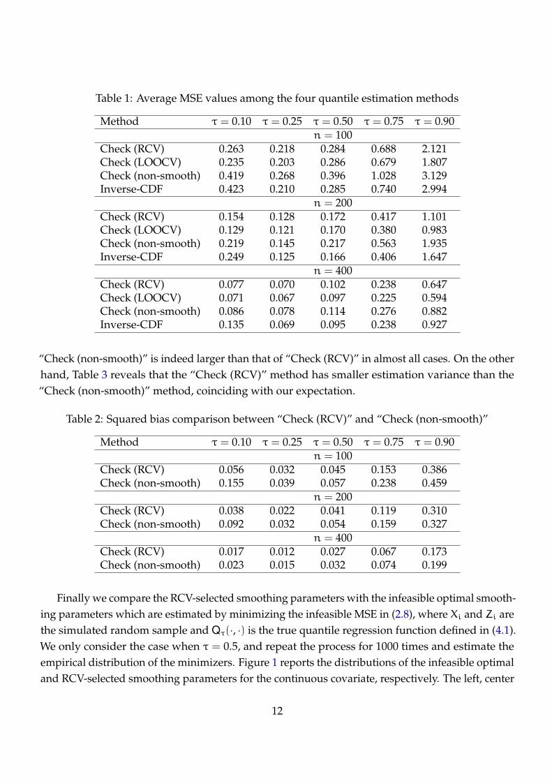
Table 1: Average MSE values among the four quantile estimation methods

Method τ = 0.10 τ = 0.25 τ = 0.50 τ = 0.75 τ = 0.90n = 100

Check (RCV) 0.263 0.218 0.284 0.688 2.121Check (LOOCV) 0.235 0.203 0.286 0.679 1.807Check (non-smooth) 0.419 0.268 0.396 1.028 3.129Inverse-CDF 0.423 0.210 0.285 0.740 2.994

n = 200Check (RCV) 0.154 0.128 0.172 0.417 1.101Check (LOOCV) 0.129 0.121 0.170 0.380 0.983Check (non-smooth) 0.219 0.145 0.217 0.563 1.935Inverse-CDF 0.249 0.125 0.166 0.406 1.647

n = 400Check (RCV) 0.077 0.070 0.102 0.238 0.647Check (LOOCV) 0.071 0.067 0.097 0.225 0.594Check (non-smooth) 0.086 0.078 0.114 0.276 0.882Inverse-CDF 0.135 0.069 0.095 0.238 0.927

“Check (non-smooth)” is indeed larger than that of “Check (RCV)” in almost all cases. On the other

hand, Table 3 reveals that the “Check (RCV)” method has smaller estimation variance than the

“Check (non-smooth)” method, coinciding with our expectation.

Table 2: Squared bias comparison between “Check (RCV)” and “Check (non-smooth)”

Method τ = 0.10 τ = 0.25 τ = 0.50 τ = 0.75 τ = 0.90n = 100

Check (RCV) 0.056 0.032 0.045 0.153 0.386Check (non-smooth) 0.155 0.039 0.057 0.238 0.459

n = 200Check (RCV) 0.038 0.022 0.041 0.119 0.310Check (non-smooth) 0.092 0.032 0.054 0.159 0.327


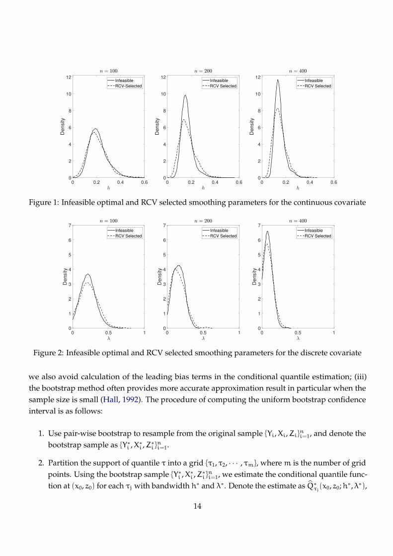
Finally we compare the RCV-selected smoothing parameters with the infeasible optimal smooth-

ing parameters which are estimated by minimizing the infeasible MSE in (2.8), where Xi and Zi are

the simulated random sample and Qτ(·, ·) is the true quantile regression function defined in (4.1).

We only consider the case when τ = 0.5, and repeat the process for 1000 times and estimate the

empirical distribution of the minimizers. Figure 1 reports the distributions of the infeasible optimal

and RCV-selected smoothing parameters for the continuous covariate, respectively. The left, center

12

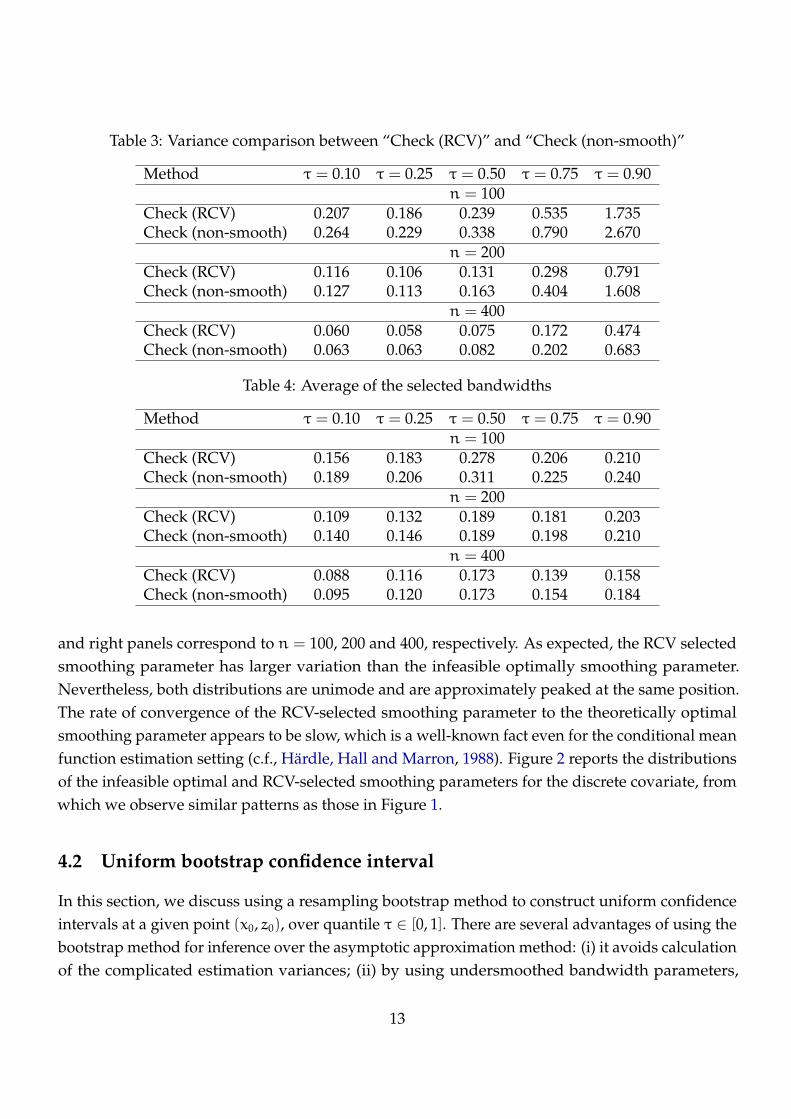
Table 3: Variance comparison between “Check (RCV)” and “Check (non-smooth)”

Method τ = 0.10 τ = 0.25 τ = 0.50 τ = 0.75 τ = 0.90n = 100




Table 4: Average of the selected bandwidths

Method τ = 0.10 τ = 0.25 τ = 0.50 τ = 0.75 τ = 0.90n = 100




and right panels correspond to n = 100, 200 and 400, respectively. As expected, the RCV selected

smoothing parameter has larger variation than the infeasible optimally smoothing parameter.

Nevertheless, both distributions are unimode and are approximately peaked at the same position.

The rate of convergence of the RCV-selected smoothing parameter to the theoretically optimal

smoothing parameter appears to be slow, which is a well-known fact even for the conditional mean

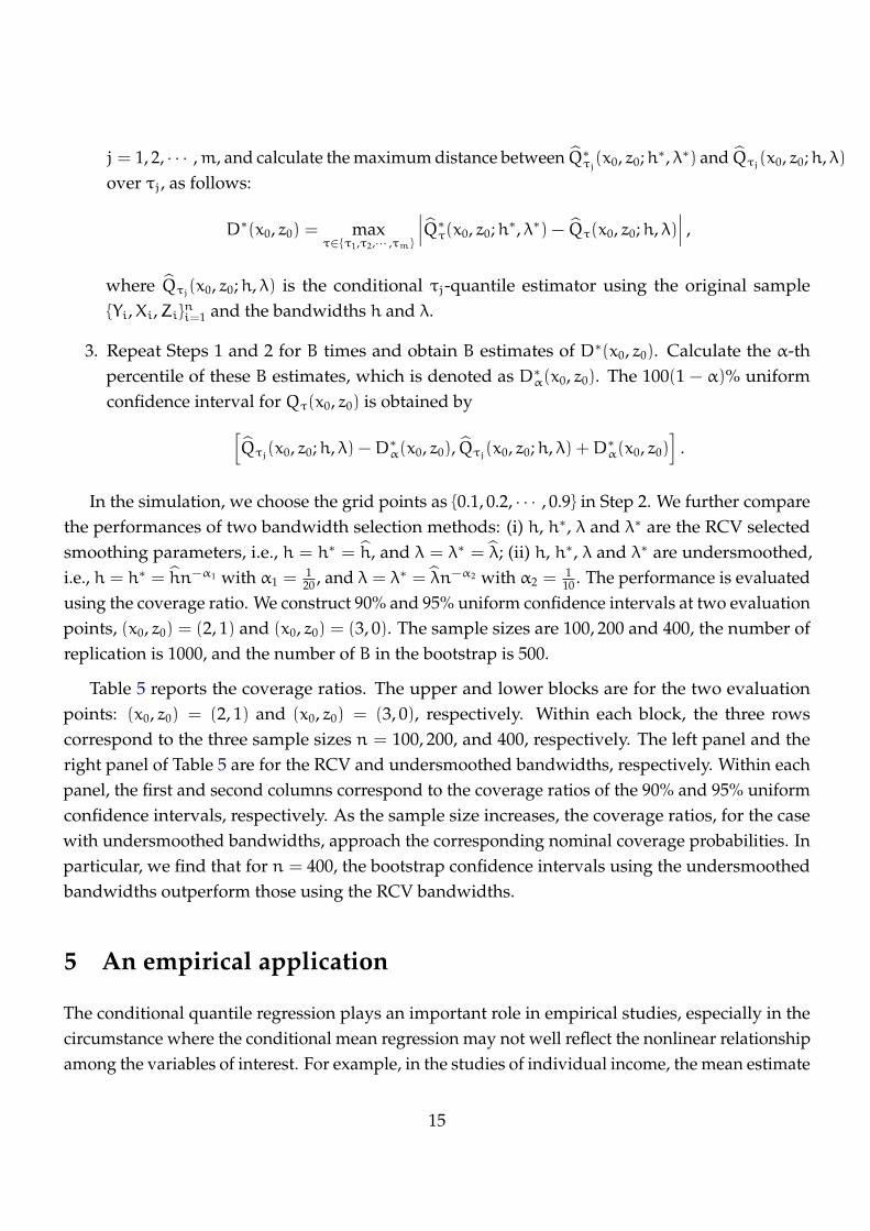
function estimation setting (c.f., Hardle, Hall and Marron, 1988). Figure 2 reports the distributions

of the infeasible optimal and RCV-selected smoothing parameters for the discrete covariate, from

which we observe similar patterns as those in Figure 1.

4.2 Uniform bootstrap confidence interval

In this section, we discuss using a resampling bootstrap method to construct uniform confidence

intervals at a given point (x0, z0), over quantile τ ∈ [0, 1]. There are several advantages of using the

bootstrap method for inference over the asymptotic approximation method: (i) it avoids calculation

of the complicated estimation variances; (ii) by using undersmoothed bandwidth parameters,

13

0 0.2 0.4 0.60

2

4

6

8

10

12

Density

Infeasible

RCV-Selected

0 0.2 0.4 0.60

2

4

6

8

10

12

Density

Infeasible

RCV Selected

0 0.2 0.4 0.60

2

4

6

8

10

12

Density

Infeasible

RCV Selected

Figure 1: Infeasible optimal and RCV selected smoothing parameters for the continuous covariate

0 0.5 10

1

2

3

4

5

6

7

Density

Infeasible

RCV Selected

0 0.5 10

1

2

3

4

5

6

7

Density

Infeasible

RCV Selected

0 0.5 10

1

2

3

4

5

6

7

Density

Infeasible

RCV Selected

Figure 2: Infeasible optimal and RCV selected smoothing parameters for the discrete covariate

we also avoid calculation of the leading bias terms in the conditional quantile estimation; (iii)

the bootstrap method often provides more accurate approximation result in particular when the

sample size is small (Hall, 1992). The procedure of computing the uniform bootstrap confidence

interval is as follows:

1. Use pair-wise bootstrap to resample from the original sample {Yi,Xi,Zi}ni=1, and denote the

bootstrap sample as {Y∗i ,X∗

i ,Z∗i }

ni=1.

2. Partition the support of quantile τ into a grid {τ1, τ2, · · · , τm}, where m is the number of grid

points. Using the bootstrap sample {Y∗i ,X∗

i ,Z∗i }

ni=1, we estimate the conditional quantile func-

tion at (x0, z0) for each τj with bandwidth h∗ and λ∗. Denote the estimate as Q∗τj(x0, z0;h∗, λ∗),

14

j = 1, 2, · · · ,m, and calculate the maximum distance between Q∗τj(x0, z0;h∗, λ∗) and Qτj

(x0, z0;h, λ)

over τj, as follows:

D∗(x0, z0) = maxτ∈{τ1,τ2,··· ,τm}

∣∣∣Q∗τ(x0, z0;h∗, λ∗) − Qτ(x0, z0;h, λ)

∣∣∣ ,

where Qτj(x0, z0;h, λ) is the conditional τj-quantile estimator using the original sample

{Yi,Xi,Zi}ni=1 and the bandwidths h and λ.

3. Repeat Steps 1 and 2 for B times and obtain B estimates of D∗(x0, z0). Calculate the α-th

percentile of these B estimates, which is denoted as D∗α(x0, z0). The 100(1 − α)% uniform

confidence interval for Qτ(x0, z0) is obtained by

[Qτj

(x0, z0;h, λ) −D∗α(x0, z0), Qτj

(x0, z0;h, λ) +D∗α(x0, z0)

].

In the simulation, we choose the grid points as {0.1, 0.2, · · · , 0.9} in Step 2. We further compare

the performances of two bandwidth selection methods: (i) h, h∗, λ and λ∗ are the RCV selected

smoothing parameters, i.e., h = h∗ = h, and λ = λ∗ = λ; (ii) h, h∗, λ and λ∗ are undersmoothed,

i.e., h = h∗ = hn−α1 with α1 =120

, and λ = λ∗ = λn−α2 with α2 =110

. The performance is evaluated

using the coverage ratio. We construct 90% and 95% uniform confidence intervals at two evaluation

points, (x0, z0) = (2, 1) and (x0, z0) = (3, 0). The sample sizes are 100, 200 and 400, the number of

replication is 1000, and the number of B in the bootstrap is 500.

Table 5 reports the coverage ratios. The upper and lower blocks are for the two evaluation

points: (x0, z0) = (2, 1) and (x0, z0) = (3, 0), respectively. Within each block, the three rows

correspond to the three sample sizes n = 100, 200, and 400, respectively. The left panel and the

right panel of Table 5 are for the RCV and undersmoothed bandwidths, respectively. Within each

panel, the first and second columns correspond to the coverage ratios of the 90% and 95% uniform

confidence intervals, respectively. As the sample size increases, the coverage ratios, for the case

with undersmoothed bandwidths, approach the corresponding nominal coverage probabilities. In

particular, we find that for n = 400, the bootstrap confidence intervals using the undersmoothed

bandwidths outperform those using the RCV bandwidths.

5 An empirical application

The conditional quantile regression plays an important role in empirical studies, especially in the

circumstance where the conditional mean regression may not well reflect the nonlinear relationship

among the variables of interest. For example, in the studies of individual income, the mean estimate

15

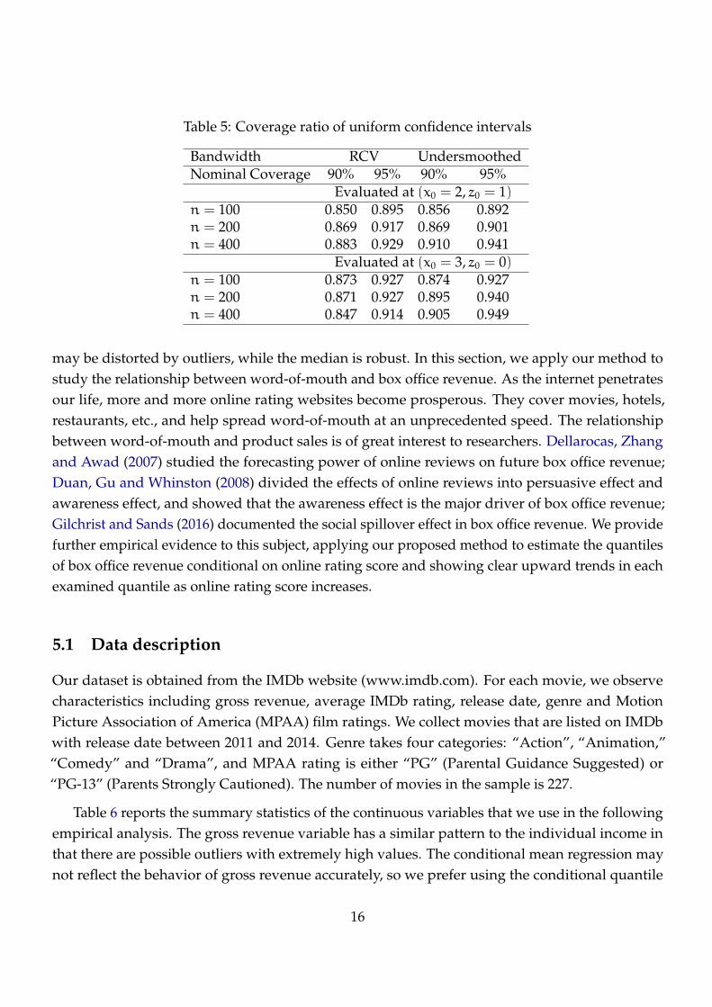
Table 5: Coverage ratio of uniform confidence intervals

Bandwidth RCV UndersmoothedNominal Coverage 90% 95% 90% 95%

Evaluated at (x0 = 2, z0 = 1)n = 100 0.850 0.895 0.856 0.892n = 200 0.869 0.917 0.869 0.901n = 400 0.883 0.929 0.910 0.941

Evaluated at (x0 = 3, z0 = 0)n = 100 0.873 0.927 0.874 0.927n = 200 0.871 0.927 0.895 0.940n = 400 0.847 0.914 0.905 0.949

may be distorted by outliers, while the median is robust. In this section, we apply our method to

study the relationship between word-of-mouth and box office revenue. As the internet penetrates

our life, more and more online rating websites become prosperous. They cover movies, hotels,

restaurants, etc., and help spread word-of-mouth at an unprecedented speed. The relationship

between word-of-mouth and product sales is of great interest to researchers. Dellarocas, Zhang

and Awad (2007) studied the forecasting power of online reviews on future box office revenue;

Duan, Gu and Whinston (2008) divided the effects of online reviews into persuasive effect and

awareness effect, and showed that the awareness effect is the major driver of box office revenue;

Gilchrist and Sands (2016) documented the social spillover effect in box office revenue. We provide

further empirical evidence to this subject, applying our proposed method to estimate the quantiles

of box office revenue conditional on online rating score and showing clear upward trends in each

examined quantile as online rating score increases.

5.1 Data description

Our dataset is obtained from the IMDb website (www.imdb.com). For each movie, we observe

characteristics including gross revenue, average IMDb rating, release date, genre and Motion

Picture Association of America (MPAA) film ratings. We collect movies that are listed on IMDb

with release date between 2011 and 2014. Genre takes four categories: “Action”, “Animation,”

“Comedy” and “Drama”, and MPAA rating is either “PG” (Parental Guidance Suggested) or

“PG-13” (Parents Strongly Cautioned). The number of movies in the sample is 227.

Table 6 reports the summary statistics of the continuous variables that we use in the following

empirical analysis. The gross revenue variable has a similar pattern to the individual income in

that there are possible outliers with extremely high values. The conditional mean regression may

not reflect the behavior of gross revenue accurately, so we prefer using the conditional quantile

16

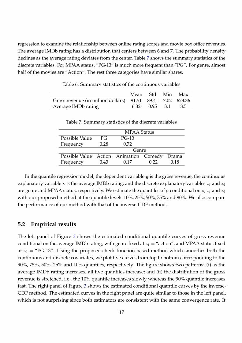
regression to examine the relationship between online rating scores and movie box office revenues.

The average IMDb rating has a distribution that centers between 6 and 7. The probability density

declines as the average rating deviates from the center. Table 7 shows the summary statistics of the

discrete variables. For MPAA status, “PG-13” is much more frequent than “PG”. For genre, almost

half of the movies are “Action”. The rest three categories have similar shares.

Table 6: Summary statistics of the continuous variables

Mean Std Min MaxGross revenue (in million dollars) 91.51 89.41 7.02 623.36Average IMDb rating 6.32 0.95 3.1 8.5

Table 7: Summary statistics of the discrete variables

MPAA StatusPossible Value PG PG-13Frequency 0.28 0.72

GenrePossible Value Action Animation Comedy DramaFrequency 0.43 0.17 0.22 0.18

In the quantile regression model, the dependent variable y is the gross revenue, the continuous

explanatory variable x is the average IMDb rating, and the discrete explanatory variables z1 and z2

are genre and MPAA status, respectively. We estimate the quantiles of y conditional on x, z1 and z2

with our proposed method at the quantile levels 10%, 25%, 50%, 75% and 90%. We also compare

the performance of our method with that of the inverse-CDF method.

5.2 Empirical results

The left panel of Figure 3 shows the estimated conditional quantile curves of gross revenue

conditional on the average IMDb rating, with genre fixed at z1 = “action”, and MPAA status fixed

at z2 = “PG-13”. Using the proposed check-function-based method which smoothes both the

continuous and discrete covariates, we plot five curves from top to bottom corresponding to the

90%, 75%, 50%, 25% and 10% quantiles, respectively. The figure shows two patterns: (i) as the

average IMDb rating increases, all five quantiles increase; and (ii) the distribution of the gross

revenue is stretched, i.e., the 10% quantile increases slowly whereas the 90% quantile increases

fast. The right panel of Figure 3 shows the estimated conditional quantile curves by the inverse-

CDF method. The estimated curves in the right panel are quite similar to those in the left panel,

which is not surprising since both estimators are consistent with the same convergence rate. It

17

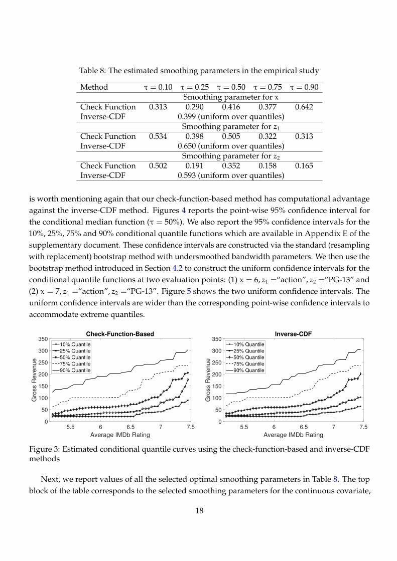
Table 8: The estimated smoothing parameters in the empirical study

Method τ = 0.10 τ = 0.25 τ = 0.50 τ = 0.75 τ = 0.90Smoothing parameter for x

Check Function 0.313 0.290 0.416 0.377 0.642Inverse-CDF 0.399 (uniform over quantiles)

Smoothing parameter for z1


Smoothing parameter for z2


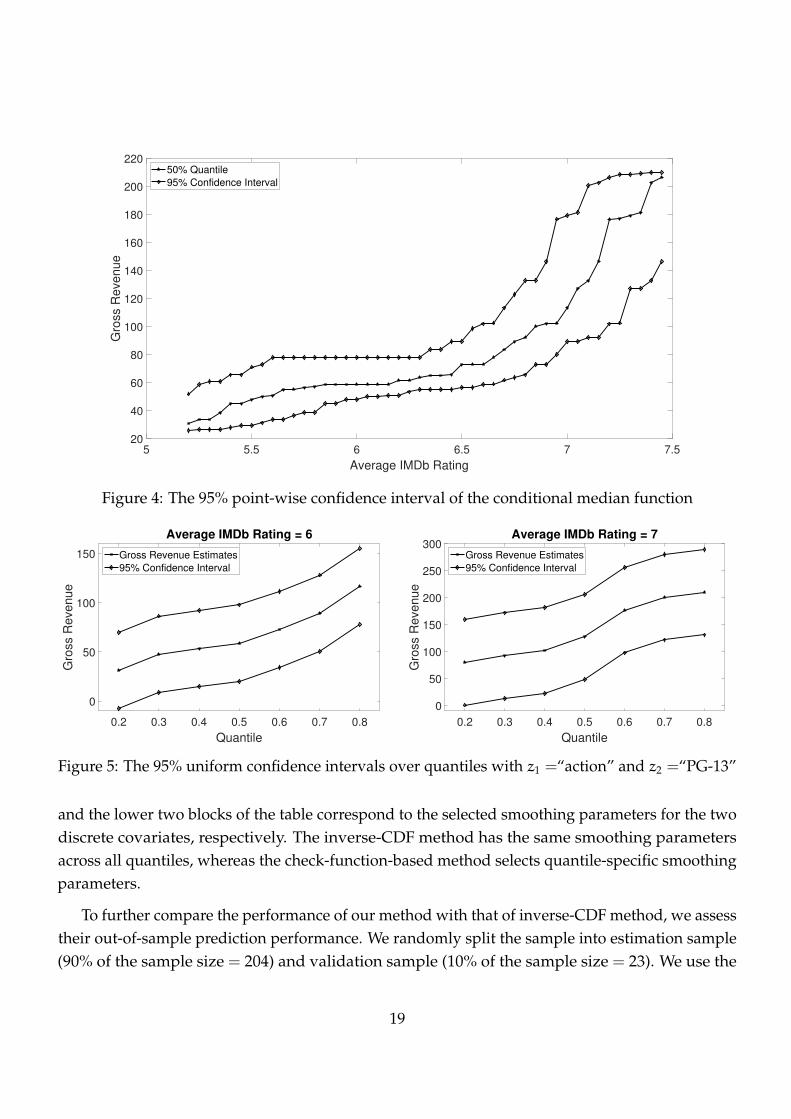
is worth mentioning again that our check-function-based method has computational advantage

against the inverse-CDF method. Figures 4 reports the point-wise 95% confidence interval for

the conditional median function (τ = 50%). We also report the 95% confidence intervals for the

10%, 25%, 75% and 90% conditional quantile functions which are available in Appendix E of the

supplementary document. These confidence intervals are constructed via the standard (resampling

with replacement) bootstrap method with undersmoothed bandwidth parameters. We then use the

bootstrap method introduced in Section 4.2 to construct the uniform confidence intervals for the

conditional quantile functions at two evaluation points: (1) x = 6, z1 =“action”, z2 =“PG-13” and

(2) x = 7, z1 =“action”, z2 =“PG-13”. Figure 5 shows the two uniform confidence intervals. The

uniform confidence intervals are wider than the corresponding point-wise confidence intervals to

accommodate extreme quantiles.

5.5 6 6.5 7 7.5

Average IMDb Rating

0

50

100

150

200

250

300

350

Gro

ss R

eve

nu

e

Check-Function-Based

10% Quantile

25% Quantile

50% Quantile

75% Quantile

90% Quantile

5.5 6 6.5 7 7.5

Average IMDb Rating

0

50

100

150

200

250

300

350

Gro

ss R

eve

nu

e

Inverse-CDF

10% Quantile

25% Quantile

50% Quantile

75% Quantile

90% Quantile

Figure 3: Estimated conditional quantile curves using the check-function-based and inverse-CDFmethods

Next, we report values of all the selected optimal smoothing parameters in Table 8. The top

block of the table corresponds to the selected smoothing parameters for the continuous covariate,

18

5 5.5 6 6.5 7 7.5

Average IMDb Rating

20

40

60

80

100

120

140

160

180

200

220

Gro

ss R

evenue

50% Quantile

95% Confidence Interval

Figure 4: The 95% point-wise confidence interval of the conditional median function

0.2 0.3 0.4 0.5 0.6 0.7 0.8

Quantile

0

50

100

150

Gro

ss R

evenue

Average IMDb Rating = 6

Gross Revenue Estimates


0.2 0.3 0.4 0.5 0.6 0.7 0.8

Quantile

0

50

100

150

200

250

300

Gro

ss R

evenue

Average IMDb Rating = 7

Gross Revenue Estimates


Figure 5: The 95% uniform confidence intervals over quantiles with z1 =“action” and z2 =“PG-13”

and the lower two blocks of the table correspond to the selected smoothing parameters for the two

discrete covariates, respectively. The inverse-CDF method has the same smoothing parameters

across all quantiles, whereas the check-function-based method selects quantile-specific smoothing

parameters.

To further compare the performance of our method with that of inverse-CDF method, we assess

their out-of-sample prediction performance. We randomly split the sample into estimation sample

(90% of the sample size = 204) and validation sample (10% of the sample size = 23). We use the

19

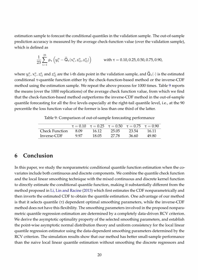
estimation sample to forecast the conditional quantiles in the validation sample. The out-of-sample

prediction accuracy is measured by the average check-function value (over the validation sample),

which is defined as

1

23

23∑

i=1

ρτ

(yoi − Qτ(x

oi , zoi1, zoi2)

)with τ = 0.10, 0.25, 0.50, 0.75, 0.90,

where yoi , xoi , zoi1 and zoi2 are the i-th data point in the validation sample, and Qτ(·) is the estimated

conditional τ-quantile function either by the check-function-based method or the inverse-CDF

method using the estimation sample. We repeat the above process for 1000 times. Table 9 reports

the means (over the 1000 replications) of the average check function value, from which we find

that the check-function-based method outperforms the inverse-CDF method in the out-of-sample

quantile forecasting for all the five levels especially at the right-tail quantile level, i.e., at the 90

percentile the loss function value of the former is less than one third of the latter.

Table 9: Comparison of out-of-sample forecasting performance

τ = 0.10 τ = 0.25 τ = 0.50 τ = 0.75 τ = 0.90Check Function 8.09 16.12 25.05 23.54 16.11Inverse-CDF 9.97 18.05 27.78 36.60 49.80

6 Conclusion

In this paper, we study the nonparametric conditional quantile function estimation when the co-

variates include both continuous and discrete components. We combine the quantile check function

and the local linear smoothing technique with the mixed continuous and discrete kernel function

to directly estimate the conditional quantile function, making it substantially different from the

method proposed in Li, Lin and Racine (2013) which first estimates the CDF nonparametrically and

then inverts the estimated CDF to obtain the quantile estimation. One advantage of our method

is that it selects quantile (τ) dependent optimal smoothing parameters, while the inverse-CDF

method does not have this flexibility. The smoothing parameters involved in the proposed nonpara-

metric quantile regression estimation are determined by a completely data-driven RCV criterion.

We derive the asymptotic optimality property of the selected smoothing parameters, and establish

the point-wise asymptotic normal distribution theory and uniform consistency for the local linear

quantile regression estimator using the data-dependent smoothing parameters determined by the

RCV criterion. The simulation results show that our method has better small-sample performance

than the naive local linear quantile estimation without smoothing the discrete regressors and

20

the inverse-CDF method. In addition, the selected smoothing parameters are very close to the

theoretically optimal ones in finite samples. Furthermore, the proposed nonparametric quantile

estimation method is used to study the relationship between box office revenues and online rating

scores. Our empirical results suggest that as the average online rating score increases, the examined

quantiles of box office revenue increases, and the higher quantile regression functions increases

faster than the lower ones.

We derive the asymptotic theory of the local linear quantile regression estimator for fixed

0 < τ < 1, see Theorems 3.1 and 3.2. A possible extension is to combine the local linear smoothing

method introduced in Section 2 with the linear interpolation technique (Qu and Yoon, 2015) to

obtain quantile regression estimates for all τ ∈ T ≡ [τ, τ], where 0 < τ < τ < 1. Specifically,

consider a set of grid points (with equal distance) arranged in the increasing order: {τ0, τ1, · · · , τrn}

with τ0 = τ and τrn = τ, where rn is a positive integer which may be divergent to infinity as n

increases. For each given τk, 0 6 k 6 rn, we minimize the loss function in (2.2) with respect to α,

and obtain the local linear estimate of the τk-quantile regression function Qτk(x0, z0), denoted by

Qτk(x0, z0;hτk

, λτk), where we make the dependence of hτ and λτ on τ explicitly. Then, we apply

the technique of linear interpolation between Qτk(x0, z0;hτk

, λτk), i.e.,

Q⋄τ(x0, z0) =

τk+1 − τ

τk+1 − τk· Qτk

(x0, z0;hτk, λτk

) +τ− τk

τk+1 − τk· Qτk+1

(x0, z0;hτk+1, λτk+1

) (6.1)

for τk 6 τ 6 τk+1. To ensure monotonicity of the estimated quantile regression curves (with

respect to τ), we may further apply the re-arrangement technique to Q⋄τ(x0, z0) defined in (6.1), see,

for example, Chernozhukov, Fernandez-Val and Galichon (2010). It would be an interesting future

topic to derive the uniform convergence result for Q⋄τ(x0, z0) using the RCV selected smoothing

parameters.

While the proposed RCV method to select the smoothing parameters has computational advan-

tage over the conventional “leave-one-out” CV method which is commonly used in practice, the

simulation results reported in Section 4 show that the latter slightly outperforms the RCV method

in finite samples (see Table 1). Therefore, a further extension of the theoretical justification of this

paper to cover the case of “leave-one-out” CV method (possibly with a different mathematical

technique) would be another important future research topic.

Acknowledgements

The authors would like to thank a Co-Editor, an Associate Editor and two anonymous reviewers

for their insightful comments that substantially improve an early version of the paper.

21

Appendix A Assumptions

Throughout the appendix, we write an ∼ bn and anP∼ bn to denote that an = bn(1 + o(1)) and an =

bn(1 + oP(1)), respectively; let an ≍ bn denote that an = O(bn) and bn = O(an) hold jointly. Below we

give some regularity conditions which are used to prove the main theoretical results of the paper.

ASSUMPTION 1. The kernel function K(·) is a Lipschitz continuous and symmetric probability density

function with a compact support [−1, 1].

ASSUMPTION 2. The sequence of {(Yi,Xi,Zi)} is composed of independent and identically distributed

(i.i.d.) random vectors.

ASSUMPTION 3. The conditional density function of ei ≡ Yi − Qτ(Xi,Zi) for given Xi = x and Zi = z,

fe(·|x, z), exists and has continuous first-order derivative at point zero. Furthermore, fe(0|x, z) is

continuous with respect to x and bounded away from infinity and zero uniformly for (x, z) ∈ Dx×Dz.

The conditional CDF of ei for given Xi = x and Zi = z, Fe(·|x, z), is continuous with respect to x. The

joint probability density function of Xi and Zi, fxz(·, ·), is bounded away from infinity and zero over

Dx ×Dz.

ASSUMPTION 4. The quantile regression function Qτ(·, z) is twice continuously differentiable on Dx.

The weight function M(·) is continuous on Dx(ǫ), and M(x) = 0 for x 6∈ Dx(ǫ), where Dx(ǫ) =

{(x1, · · · , xp) : cj + ǫ 6 xj 6 cj − ǫ, j = 1, · · · ,p} with ǫ being a very small positive constant.

ASSUMPTION 5. (i) For (h, λ) ∈ Hm with h = (h1, · · · ,hp)⊺

and λ = (λ1, · · · , λq)⊺

, hj → 0 and λj → 0 as

n → ∞.

(ii) Letting H =∏p

j=1 hj, for (h, λ) ∈ Hm,∑p

j=1 h2j +

∑qj=1 λj = o

((1

n1/2H

)∧(

lognnH

)1/3)

, and

lognnH = o

(∑pj=1 h

2j +

∑qj=1 λj

).

(iii) The number of grid points in Hm, Lm, diverges at a polynomial rate of m, and in addition,

γm = o(m−2/(4+p)).

Assumption 1 imposes some mild conditions on the continuous kernel function in the nonparametric

kernel-based smoothing, and several commonly-used kernel functions such as the uniform kernel and the

Epanechnikov kernel satisfy these conditions (c.f., Fan and Gijbels, 1996). In Assumption 2, we impose the

i.i.d. condition on the observations, a commonly-used setting in the literature on nonparametric estimation

with mixed discrete and continuous data (c.f., Li and Racine, 2004). The asymptotic results of this paper

can be generalized to the general stationary and weakly dependent processes at the cost of more lengthy

proofs. There is no moment condition on ei to estimate the conditional quantile regression, indicating that

the error distribution is allowed to have heavy tails. Assumptions 3 and 4 give some smoothness conditions

on the (conditional) density functions, the weight function and the quantile regression function, which are

often imposed in studying asymptotic behavior of nonparametric kernel-based estimators. Assumption 5

imposes some standard restrictions on the smoothing parameters. Assumption 5(ii) is crucial to guarantee

22

that the second term on the right hand side of (2.7) is the asymptotic leading term to determine the optimal

bandwidth vectors and Assumption 5(iii) indicates that the grid points are sufficiently dense in the set Hm.

The theoretically optimal bandwidths h0 and λ0 satisfy Assumption 5(ii), and by Assumption 5(iii), there

exists a grid point in Hm which is sufficiently close to (h0, λ0).

Appendix B Proofs of the main results

In this appendix, we give the detailed proofs of the main theoretical results in Sections 2 and 3. In

order to simplify the presentation, we first introduce some notation. For x = (x1, · · · , xp)⊺ ∈ Dx and

z = (z1, · · · , zq)⊺ ∈ Dz, we let

∆ni(α,β; x, z) =1√nH

un(α; x, z) +

p∑

j=1

vn,j(βj; x, z)

(Xi,j − xj

hj

)

with un(α; x, z) =√nH [α− Qτ(x, z)] and vn,j(βj; x, z) =

√nHhj

[βj − Q′

τ,j(x, z)], and bi(x, z) = Qτ(Xi,Zi)−

Qτ(x, z) −∑p

j=1 Q′τ,j(x, z)(Xi,j − xj). With the above notation, it is easy to see that

Yi − α− (Xi − x)⊺

β = ei − ∆ni(α,β; x, z) + bi(x, z).

B.1 Proof of Theorem 2.1

Let ζM1,h,λ(Xj,Zj) = QM1(Xj,Zj;h, λ) − Qτ(Xj,Zj) with QM1

(Xj,Zj;h, λ) defined as in (2.3). Then

CV(h, λ) =1

n−m

n∑

j=m+1

ρτ

(ej + Qτ(Xj,Zj) − QM1

(Xj,Zj;h, λ))M(Xj)

≡ CV∗ + CV2(h, λ), (B.1)

where CV∗ (defined in Theorem 2.1) does not rely on the smoothing parameters h and λ (so would not play

any role in choosing the optimal bandwidth vectors), and

CV2(h, λ) =1

n−m

n∑

j=m+1

[ρτ(ej − ζM1,h,λ(Xj,Zj)

)− ρτ(ej)

]M(Xj).

We only need to study CV2(h, λ). Using the following identity result (e.g., Knight, 1998):

ρτ(u− v) − ρτ(u) = v (I{u 6 0}− τ) +

∫v

0(I{u 6 w}− I{u 6 0})dw, (B.2)

23

we have

ρτ(ej− ζM1,h,λ(Xj,Zj)

)−ρτ(ej) = ζM1,h,λ(Xi,Zi)

(I{ej 6 0}− τ

)+

∫ζM1,h,λ(Xj,Zj)

0

(I{ej 6 w}− I{ej 6 0}

)dw.

Define

CV21(h, λ) =1

n−m

n∑

j=m+1

ζM1,h,λ(Xj,Zj)(I{ej 6 0}− τ

)M(Xj),

CV22(h, λ) =1

n−m

n∑

j=m+1

M(Xj)

∫ζM1,h,λ(Xj,Zj)

0

(I{ej 6 w}− I{ej 6 0}

)dw.

Then, we readily have that CV2(h, λ) = CV21(h, λ) + CV22(h, λ).

We first derive the asymptotic order for CV22(h, λ) and show that it is the asymptotic leading term

of CV2(h, λ). As m ≍ n, by Propositions C.1 and C.2 in Appendix C of the supplemental document and

Assumption 5(ii), we have

CV22(h, λ) = CV∗22(h, λ) +OP

(χ

5/21 (h) + χ1(h)χ

3/22 (h, λ) + χ3(h, λ)

)

= CV∗22(h, λ) + oP

(χ2

2(h, λ) +1

mH

)(B.3)

uniformly over (h, λ) ∈ Hm, where χ1(h) = (logn)1/2(nH)−1/2, χ2(h, λ) =∑p

j=1 h2j +

∑qj=1 λj, χ3(h, λ) =

(logn/n)1/2[χ1(h) + χ2(h, λ)], and

CV∗22(h, λ) =

1

2(n−m)

n∑

j=m+1

[ζ∗M1,h,λ(Xj,Zj)

]2fe(0|Xj,Zj)M(Xj) (B.4)

in which ζ∗M1,h,λ(Xj,Zj) = f−1(Xj,Zj)WM1,h,λ(Xj,Zj), f(x, z) = fxz(x, z)fe(0|x, z), and

WM1,h,λ(Xj,Zj) = m−1m∑

i=1

ηi(Xj,Zj)Kh(Xi − Xj)Λλ(Zi,Zj)

with ηi(x, z) = τ− I {ei 6 −bi(x, z)}.

Letting ηi = τ− I(ei 6 0), we rewrite WM1,h,λ(Xj,Zj) as

WM1,h,λ(Xj,Zj) =1

m

m∑

i=1

[ηi(Xj,Zj) − ηi

]Kh(Xi − Xj)Λλ(Zi,Zj) +

1

m

m∑

i=1

ηiKh(Xi − Xj)Λλ(Zi,Zj)

≡ WM1,h,λ(Xj,Zj) + WM1,h,λ(Xj,Zj). (B.5)

Define BM1,h,λ(Xj,Zj) = f−1(Xj,Zj)WM1,h,λ(Xj,Zj) and VM1,h,λ(Xj,Zj) = f−1(Xj,Zj)WM1,h,λ(Xj,Zj), by

24

(B.4) and (B.5), we readily have that

CV∗22(h, λ) =

1

2(n−m)

n∑

j=m+1

B2M1,h,λ(Xj,Zj)fe(0|Xj,Zj)M(Xj) +

1

2(n−m)

n∑

j=m+1

V2M1,h,λ(Xj,Zj)fe(0|Xj,Zj)M(Xj) +

1

n−m

n∑

j=m+1

BM1,h,λ(Xj,Zj)VM1,h,λ(Xj,Zj)fe(0|Xj,Zj)M(Xj)

≡ CV∗22,B(h, λ) + CV

∗22,V(h, λ) + CV

∗22,BV(h, λ). (B.6)

We consider the three terms on the right hand side of (B.6) separately. We start with CV∗22,B(h, λ). Note

that

1

2(n−m)

n∑

j=m+1

B2M1,h,λ(Xj,Zj)fe(0|Xj,Zj)M(Xj)

=1

2m2(n−m)

n∑

j=m+1

fe(0|Xj,Zj)M(Xj)

f2(Xj,Zj)

m∑

i1=1

m∑

i2=1

[ηi1

(Xj,Zj) − ηi1

] [ηi2

(Xj,Zj) − ηi2

]

Kh(Xi1− Xj)Λλ(Zi1

,Zj)Kh(Xi2− Xj)Λλ(Zi2

,Zj)

=1

2m2(n−m)

n∑

j=m+1

fe(0|Xj,Zj)M(Xj)

f2(Xj,Zj)

m∑

i=1

[ηi(Xj,Zj) − ηi

]2K2

h(Xi − Xj)Λ2λ(Zi,Zj) +

1

2m2(n−m)

n∑

j=m+1

fe(0|Xj,Zj)M(Xj)

f2(Xj,Zj)

m∑

i1=1

m∑

i2=1, 6=i1

[ηi1

(Xj,Zj) − ηi1

] [ηi2

(Xj,Zj) − ηi2

]


,Zj)Kh(Xi2− Xj)Λλ(Zi2

,Zj)

≡ CV∗22,B,1(h, λ) + CV

∗22,B,2(h, λ). (B.7)

By (B.7) and Proposition C.3, we have

CV∗22,B(h, λ) =

1

2(n−m)

n∑

j=m+1

b2(Xj,Zj;h, λ)fe(0|Xj,Zj)M(Xj) + oP

(χ2

2(h, λ) +1

mH

)(B.8)

uniformly over (h, λ) ∈ Hm. Next, we consider CV∗22,V(h, λ) on the right hand side of (B.6). Note that

1

2(n−m)

n∑

j=m+1

V2M1,h,λ(Xj,Zj)fe(0|Xj,Zj)M(Xj)

=1

2m2(n−m)

n∑

j=m+1

fe(0|Xj,Zj)M(Xj)

f2(Xj,Zj)

m∑

i1=1

m∑

i2=1

ηi1ηi2


,Zj)


,Zj)

25

=1

2m2(n−m)

n∑

j=m+1

fe(0|Xj,Zj)M(Xj)

f2(Xj,Zj)

m∑

i=1

η2iK2

h(Xi − Xj)Λ2λ(Zi,Zj) +

1

2m2(n−m)

n∑

j=m+1

fe(0|Xj,Zj)M(Xj)

f2(Xj,Zj)

m∑

i1=1

m∑

i2=1,6=i1

ηi1ηi2


,Zj)


,Zj)

≡ CV∗22,V ,1(h, λ) + CV

∗22,V ,2(h, λ). (B.9)

By (B.9) and Proposition C.4, we may show that

CV∗22,V(h, λ) =

1

2(n−m)

n∑

j=m+1

σ2m(Xj,Zj;h, λ)fe(0|Xj,Zj)M(Xj) + oP

(1

mH

)(B.10)

uniformly over (h, λ) ∈ Hm. By Proposition C.5, we have

CV∗22,BV(h, λ) = oP

(χ2

2(h, λ) +1

mH

)(B.11)

uniformly over (h, λ) ∈ Hm. Then, with (B.3), (B.6), (B.8), (B.10) and (B.11), we can prove that

CV22(h, λ) =1

2(n−m)

n∑

j=m+1

[b2(Xj,Zj;h, λ) + σ2

m(Xj,Zj;h, λ)]fe(0|Xj,Zj)M(Xj) + s.o.

=1

2E{[b2m(Xi,Zi;h, λ) + σ2


}+ s.o. (B.12)

uniformly over (h, λ) ∈ Hm.

Finally, following the proof of Proposition C.2, we may show that

CV21(h, λ) = OP (χ3(h, λ)) = oP

(χ2

2(h, λ) +1

mH

)(B.13)

uniformly over (h, λ) ∈ Hm, where χ3(h, λ) is defined as in (B.3). By (B.12) and (B.13), we complete the

proof of (2.7) in Theorem 2.1. �


Let h0m,j = a0

j ·m−1/(4+p) for j = 1, · · · ,p, and λ0m,k = d0

k ·m−2/(4+p) for k = 1, · · · ,q. Then, we readily

have that h0j = h0

m,j ·(mn

)1/(4+p)for j = 1, · · · ,p, and λ0

k = λ0m,k ·

(mn

)2/(4+p)for k = 1, · · · ,q. By (2.6), we

only need to prove that hm,j − h0m,j = oP(h

0m,j) for j = 1, 2, · · · ,p, and λm,k − λ0

m,k = oP(λ0m,k) for k =

1, 2, · · · ,q, where hm,j is the j-th element of hm and λm,k is the k-th element of λm.

From the asymptotic representation of the CV function in Theorem 2.1, the term CV∗ does not rely on

the bandwidth vectors h and λ. The second term on the right hand side of (2.7) is the asymptotic leading

26

term for the optimal bandwidth selection. Therefore, the optimal bandwidth vectors hm and λm satisfy that

hm = h⋄m + oP(h

⋄m) and λm = λ⋄m + oP(λ

⋄m), where h⋄

m and λ⋄m are the bandwidth vectors that minimize

the second term on the right hand side of (2.7) uniformly over (h, λ) ∈ Hm. Note that the latter equals to12 · MSE

LM2

(h, λ), see the definition in (2.9). Under the assumption that there exist uniquely determined

a0j > 0, j = 1, · · · ,p, and d0

k > 0, k = 1, · · · ,q, that minimize g(a,d) defined in (2.10), using Assumption

5(iii), we must have that h⋄m = h0

m + o(h0m) and λ⋄m = λ0

m + o(λ0m), where h0

m =(h0m,1, · · · ,h0

m,p

)⊺

and

λ0m =

(λ0m,1, · · · , λ0

m,q

)⊺

. This completes the proof of Theorem 2.2. �


Let ζ(x0, z0;h, λ) = (nH)1/2[Qτ (x0, z0;h, λ) − Qτ(x0, z0)

], where we make the dependence of the local

linear quantile estimators on the bandwidths h and λ explicit. We first derive the asymptotic normality

for ζ(x0, z0;h, λ) when the bandwidth vectors h and λ are chosen as the deterministic optimal bandwidths

defined in Theorem 2.2, i.e., h = h0, λ = λ0 and H0 =∏p

k=1 h0k. By Proposition C.1, we have the following

Bahadur representation:

ζ(x0, z0;h0, λ0) =Wn(x0, z0;h0, λ0)

f(x0, z0)(1 + oP(1)), (B.14)

where f(x0, z0) = fxz(x0, z0)fe(0|x0, z0) and

Wn(x0, z0;h0, λ0) =H0

√nH0

n∑

i=1

ηi(x0, z0)Kh0(Xi − x0)Λλ0(Zi, z0).

Thus, to establish the asymptotic distribution theory of ζ(x0, z0;h0, λ0), we only need to derive the limiting

distribution of Wn(x0, z0;h0, λ0).

Let Wn(x0, z0;h0, λ0) be defined as Wn(x0, z0;h0, λ0) but with ηi(x0, z0) replaced by ηi = τ − I {ei 6 0}.

Then, we have

Wn(x0, z0;h0, λ0) − E[Wn(x0, z0;h0, λ0)

]

= Wn(x0, z0;h0, λ0) − E

[Wn(x0, z0;h0, λ0)

]+Wn(x0, z0;h0, λ0) − Wn(x0, z0;h0, λ0) −

E

[Wn(x0, z0;h0, λ0) − Wn(x0, z0;h0, λ0)

]. (B.15)

Note that

Var

[Wn(x0, z0;h0, λ0) − Wn(x0, z0;h0, λ0)

]

6 E

[∣∣∣Wn(x0, z0;h0, λ0) − Wn(x0, z0;h0, λ0)∣∣∣2]

= E

{

E

[∣∣∣Wn(x0, z0;h0, λ0) − Wn(x0, z0;h0, λ0)∣∣∣2 ∣∣∣(Xn,Zn)

]}

27

= O

(H0

n

n∑

i=1

E

{

K2h0(Xi − x0)Λ

2λ0(Zi, z0)E

[(ηi(x0, z0) − ηi)

2∣∣∣(Xn,Zn)

]})

= o

(1

nH0

n∑

i=1

E

[K2

(Xi − x0

h0

)Λ

2λ0(Zi, z0)

])= o(1), (B.16)

where Xn = σ(X1, · · · ,Xn) and Zn = σ(Z1, · · · ,Zn). This implies that it is sufficient to show

Wn(x0, z0;h0, λ0) − E

[Wn(x0, z0;h0, λ0)

]d−→ N [0,V⋆(x0, z0)] , (B.17)

where V⋆(x0, z0) = τ(1 − τ)νp0 fxz(x0, z0). By the classical Central Limit Theorem for the i.i.d. random

variables, we can complete the proof of (B.17). In view of (B.15)–(B.17), we have that

Wn(x0, z0;h0, λ0) − E[Wn(x0, z0;h0, λ0)

] d−→ N [0,V⋆(x0, z0)] . (B.18)

Meanwhile, by some elementary calculations, one can prove that

1√nH0

E[Wn(x0, z0;h0, λ0)

]

f(x0, z0)∼ b(x0, z0;h0, λ0). (B.19)

By (B.18) and (B.19), we readily have that

ζ(x0, z0;h0, λ0) −√nH0b(x0, z0;h0, λ0)

d−→ N [0,V(x0, z0)] , (B.20)

where V(x0, z0) is defined as in (3.1).

Let a = (a1, · · · ,ap)⊺

and d = (d1, · · · ,dq)⊺

with aj = hj · n1/(4+p) and dk = λk · n2/(4+p) as defined

in Section 2. Similarly, let a = (a1, · · · , ap)⊺

and d =(d1, · · · , dq

)⊺

with aj = hj · n1/(4+p) and dk =

λk · n2/(4+p), and let a0 =(a0

1, · · · ,a0p

)⊺and d0 =

(d0

1, · · · ,d0q

)⊺with a0

j and d0k defined as in Theorem 2.2.

Define

ζ(x0, z0;a,d) = ζ(x0, z0;h, λ), b(x0, z0;a,d) = b(x0, z0;h, λ).

when h = a · n−1/(4+p) and λ = d · n−2/(4+p). Let Sc1(a0) and Sc2(d

0) be two neighborhoods of a0 and d0

with radius c1 > 0 and c2 > 0, respectively. Furthermore, let A be a set of grid points a(k) and D a set of

grid points d(k) such that [h(k), λ(k)] ∈ Hm with h(k) = a(k) ·m−1/(4+p) and λ(k) = d(k) ·m−2/(4+p). By

Proposition C.1 in Appendix C, one can show that

ζ(x0, z0;a,d) =Wn(x0, z0;a,d)

f(x0, z0)+ oP(1) (B.21)

uniformly over a ∈ A and d ∈ D, where Wn(x0, z0;a,d) = Wn(x0, z0;h, λ). Define

Wcn(x0, z0;a,d) = Wn(x0, z0;a,d) − E

[Wn(x0, z0;a,d)

],

28

and Sc1(a0) = Sc1

(a0) ∩ A and Sc2(d0) = Sc2(d

0) ∩ D. With (B.21), Theorem 2.2, the definition of the RCV

selected smoothing parameters, and Theorem 3.1 in Li and Li (2010), we only have to show that

E

[∣∣∣Wcn(x0, z0;a,d) −W

cn(x0, z0;a′,d′)

∣∣∣2]6 c3 · ‖a− a′‖2, (B.22)

where a,a′ ∈ Sc1(a0), d,d′ ∈ Sc2(d

0) and c3 is a positive constant, and

E[Wn(x0, z0;a,d)

]

f(x0, z0)−√nH · b(x0, z0;a,d) = o(1) (B.23)

uniformly over a ∈ Sc1(a0) and d ∈ Sc2(d

0). The proof of (B.23) is straightforward as its left hand wide is

non-random and one can use the standard Taylor expansion of the quantile regression function to prove this

result. We therefore only need to prove (B.22).

Without loss of generality, we consider p = 1 and define

i(x0, z0;a,d) = ηi(x0, z0)K

(Xi − x0

h

)Λλ(Zi, z0)

with h = a · n−1/(4+p) and λ = d · n−2/(4+p). Note that

E

{[i(x0, z0;a,d) −i(x0, z0;a′,d′)

]2}

=

∫

E[η2i(x0, z0)|Xi = x,Zi = z0

] [K

(x− x0

h

)− K

(x− x0

h′

)]2

dx+O

(q∑

k=1

λk +

q∑

k=1

λ′k

)

= h

∫

E[η2i(x0, z0)|Xi = x0 + hw,Zi = z0

] [K (w) − K

(hw/h′

)]2dw+O

(q∑

k=1

λk +

q∑

k=1

λ′k

)

6 c4h[1 − (h/h′)

]2= c4[a/(a

′)2](a− a′)2, (B.24)

where h′ = a′ · n−1/(4+p) and λ′ = d′ · n−2/(4+p) and c4 is a positive constant. Using (B.24) and following

the argument in the proof of Example 4.1 in Li and Li (2010), one can readily establish (B.22). This completes

the proof of Theorem 3.1. �


Without loss of generality, we let p = 1 and q = 1. Let(h0, λ0

)and

(h, λ)

be the deterministic optimal and

RCV selected bandwidth vectors, respectively. Define

Sε(h0, λ0) =

{

(h, λ) ∈ Hn :

∣∣∣∣h− h0

h0

∣∣∣∣ < ε,

∣∣∣∣λ− λ0

λ0

∣∣∣∣ < ε

}

,

29

where Hn is a set of grid points [h(k), λ(k)] such that[(n/m)1/(4+p)h(k), (n/m)2(4+p)λ(k)

]∈ Hm. Let a0

and d0 satisfy h0 = a0 · n−1/5 and λ0 = d0 · n−2/5 and define

Sε(a0,d0) =

{(a,d) : a ∈ A, d ∈ D,

∣∣a− a0∣∣ < ε,

∣∣d− d0∣∣ < ε

},

where A and D are defined as in the proof of Theorem 3.1. By Theorem 2.2, for any ε > 0, we readily have

that

P

((h, λ)∈ Sε(h

0, λ0))→ 1 and P

((a, d

)∈ Sε(a

0,d0))→ 1, (B.25)

where a and d are defined such that h = a · n−1/5 and λ = d · n−2/5.

For notational simplicity, we let Qτ(x, z;a,d) = Qτ(x, z;h, λ), where h = an−1/5 and λ = dn−2/5. With

(B.25), it is sufficient to prove that

P

(sup

(a,d)∈Sε(a0,d0)

supx∈Dx(ǫ)

∣∣∣Qτ(x, z;a,d) − Qτ(x, z)∣∣∣ > c5 · ιn

)→ 0, (B.26)

where c5 is a sufficiently large positive constant and ιn = n−2/5 log1/2 n. Combining Proposition C.1 and

the proof of Example 2.1 in Li and Li (2010), we readily have the following Bahadur representation:

Qτ(x, z;a,d) − Qτ(x, z) = f−1(x, z)wn(x, z;a,d)(1 + oP(1)), (B.27)

uniformly over x ∈ Dx(ǫ) and (a,d) ∈ Sε(a0,d0), where

wn(x, z;a,d) =1

(nh)1/2Wn(x, z;a,d) =

1

nh

n∑

i=1

ηi(x, z)K

(Xi − x

h

)Λλ(Zi, z)

with h = an−1/5 and λ = dn−2/5. By Assumption 3, f(x, z) is strictly larger than a positive constant

uniformly over x and z. On the other hand, we may prove that

sup(a,d)∈Sε(a0,d0)

supx∈Dx(ǫ)

|E [wn(x, z;a,d)]| = O(n−2/5) = o(ιn). (B.28)

Hence, by (B.27) and (B.28), in order to prove (B.26), we only need to show that


supx∈Dx(ǫ)

|wn(x, z;a,d) − E [wn(x, z;a,d)]| = OP(ιn). (B.29)

Consider covering the set Dx(ǫ) by some disjoint intervals D1, · · · ,DL1. Denote the center point of Dl

by xl and let the radius of Dl be of order ιnn−2/5. Then, the order of the number L1 is ι−1

n n2/5. Let L2 be the

number of grid points in Sε(a0,d0) which diverges at a polynomial rate of n by Assumption 5(iii). Note that


supx∈Dx(ǫ)

|wn(x, z;a,d) − E [wn(x, z;a,d)]|

30

6 max16l16L1

max16l26L2

|wn(xl1, z;al2

,dl2) − E [wn(xl1

, z;al2,dl2

)]|+

max16l16L1

max16l26L2

supx∈Dl1

|wn(x, z;al2,dl2

) −wn(xl1, z;al2

,dl2)|+

max16l16L1

max16l26L2

supx∈Dl1

|E [wn(x, z;al2,dl2

)] − E [wn(xl1, z;al2

,dl2)]| , (B.30)

where (al,dl), 1 6 l 6 L2, are the grid points in the set Sε(a0,d0). As the radius of Dl has the order of

ιnn−2/5, by the smoothness condition on K(·) in Assumption 1, we may show that

max16l16L1

max16l26L2

supx∈Dl1

|wn(x, z;al2,dl2

) −wn(xl1, z;al2

,dl2)| = OP(ιn) (B.31)

and

max16l16L1

max16l26L2

supx∈Dl1

|E [wn(x, z;al2,dl2

)] − E [wn(xl1, z;al2

,dl2)]| = O(ιn). (B.32)

On the other hand, by the Bonferroni inequality and Bernstein inequality for independent sequence (e.g.,

van der Vaart and Wellner, 1996), we can prove that

P

(max

16l16L1

max16l26L2

|wn(xl1, z;al2

,dl2) − E [wn(xl1

, z;al2,dl2

)]| > c5ιn

)

6

L1∑

l1=1

L2∑

l2=1

P (|wn(xl1, z;al2

,dl2) − E [wn(xl1

, z;al2,dl2

)]| > c5ιn)

6 O (L1 · L2 · exp {−c5 logn}) = o(1), (B.33)

where c5 would be a sufficiently large positive constant if c5 is large enough. Hence, we have

max16l16L1

max16l26L2

|wn(xl1, z;al2

,dl2) − E [wn(xl1

, z;al2,dl2

)]| = OP(ιn). (B.34)

By (B.30)–(B.32) and (B.34), we can prove (B.29), completing the proof of (3.3) in Theorem 3.2. �

B.5 Estimators of bias and variance

In this appendix, we discuss the construction of the estimators of local linear quantile estimation bias and

variance. Following the discussion in Section 3, the estimator of b(x0, z0; h, λ) can be obtained by replacing

unknown functions by their consistent estimates as follows

b(x0, z0; h, λ) =µ2

2

p∑

j=1

h2jQ

′′τ,j(x0, z0) +

∑

z1∈Dz

q∑

k=1

Ik(z1, z0)λkf(x0, z1)

f(x0, z0)

[Qτ(x0, z1) − Qτ(x0, z0)

],

31

where f(x0, z0) = fe(0|x0, z0)fxz(x0, z0) with

fe(0|x0, z0) =

∑ni=1 Kh0

(ei)Kh(Xi − x0)Λλ(Zi, z0)∑n

i=1 Kh(Xi − x0)Λλ(Zi, z0), (B.35)

fxz(x0, z0) =1

nH

n∑

i=1

Kh(Xi − x0)Λλ(Zi, z0), (B.36)

Kh0(ei) = h−1

0 K (ei/h0), ei = Yi − Qτ(Xi,Zi; h, λ), the bandwidth h0 in (B.35) can be determined by the rule

of thumb: h0 = sen−1/(5+p) with se being the sample standard deviation of ei, and Q′′

τ,j(x0, z0) is the j-th

diagonal element of the p × p matrix Γ. The matrix Γ, along with α and β, is defined by minimizing the

following objective function (e.g., Cheng and Peng, 2002):

n∑

i=1

ρτ

(Yi − α− (Xi − x0)

⊺

β− (1

2)(Xi − x0)

⊺

Γ(Xi − x0)

)Kh(Xi − x0)Λλ(Zi, z0).

The consistent estimator of V(x0, z0) is given by

V(x0, z0) =τ(1 − τ)ν

p0[

fe(0|x0, z0)]2

fxz(x0, z0)

,

where fe(0|x0, z0) and fxz(x0, z0) are defined in (B.35) and (B.36), respectively.

References

Belloni, A. and Chernozhukov, V. (2011). l1-penalized quantile regression in high-dimensional sparse models.

Annals of Statistics, 39, 82–130.

Belloni, A., Chernozhukov, V., Chetverikov, D. and Fernandez-Val, I. (2019). Conditional quantile processes

based on series or many regressors. Journal of Econometrics, 213, 4–29.

Cai, Z. (2002). Regression quantile for time series. Econometric Theory, 18, 169–192.

Cai, Z. and Xiao, Z. (2012). Semiparametric quantile regression estimation in dynamic models with partially

varying coefficients. Journal of Econometrics, 167, 413–425.

Cai, Z. and Xu, X. (2008). Nonparametric quantile estimations for dynamic smooth coefficient models.

Journal of the American Statistical Association, 103, 1596–1608.

Calonico, E., Cattaneo, M.D. and Titiunik, R. (2014). Robust nonparametric confidence intervals for

regression-discontinuity designs. Econometrica 82, 2295-2326.

Calonico, E., Cattaneo, M.D. and and Farrell, M.H. (2018). On the effect of bias estimation on coverage

accuracy in nonparametric inference. Journal of American Statistical Association, 113, 767-779.

32

Chen, Z., Fan, J. and Li, R. (2018). Error variance estimation in ultrahigh dimensional additive models.

Journal of the American Statistical Association, 113, 315–327.

Cheng, M. and Peng, L. (2002). Regression modeling for nonparametric estimation and distribution and

quantile functions. Statistica Sinica, 12, 1043–1060.

Chernozhukov, V., Fernandez-Val, I. and Galichon, A. (2010). Quantile and probability curves without

crossing. Econometrica, 78, 1093–1125.

Chiang, H.D., Hsu, Y.C. and Sasaki, Y. (2019). Robust uniform inference for quantile treatment effects in

regression discontinuity designs. Journal of Econometrics, 211, 589–618.

Chiang, H.D. and Sasaki, Y. (2019). Causal inference by quantile regression kink designs. Journal of Econo-

metrics, 210, 405–433.

Dellarocas, C., Zhang, X. and Awad, N. F. (2007). Exploring the value of online product reviews in forecasting

sales: The case of motion pictures. Journal of Interactive Marketing, 21(4), 23–45.

Duan, W., Gu, B. and Whinston, A. B. (2008). Do online reviews matter? - An empirical investigation of

panel data. Decision Support Systems, 45(4), 1007–1016.

Escanciano, J. C. and Goh, C. (2014). Specification analysis of linear quantile models. Journal of Econometrics,

178, 495–507.

Escanciano, J. C. and Velasco, C. (2010). Specification tests of parametric dynamic conditional quantiles.

Journal of Econometrics, 159, 209–221.

Fan J. and Gijbels, I. (1996). Local Polynomial Modelling and Its Applications. Chapman and Hall.

Fan, J., Guo, S. and Hao, N. (2012). Variance estimatino using refitted cross-validation in ultrahigh dimen-

sional regression. Journal of the Royal Statistical Society Series B, 74, 37–65.

Galvao, A. (2011) Quantile regression for dynamic panel data with fixed effects. Journal of Econometrics,

164, 142–157.

Galvao, A., Lamarche, C. and Lima, L. (2013). Estimation of censored quantile regression for panel data with

fixed effects. Journal of the American Statistical Association, 108, 1075–1089.

Gilchrist, D. S. and Sands, E. G. (2016). Something to talk about: Social spillovers in movie consumption.

Journal of Political Economy, 124(5), 1339–1382.

Green, P. J. and Silverman, B. W. (1994). Nonparametric Regression and Generalized Linear Models: A

Roughness Penalty Approach. Monographs on Statistics and Applied Probability 58, Chapman and Hall.

Guerre, E. and Sabbah, C. (2012). Uniform bias study and Bahadur representation for local polynomial

estimators of the conditional quantile function. Econometric Theory, 28, 87–129.

Hall, P. (1992). The Bootstrap and Edgeworth Expansion. Springer.

33

Hardle, W., Hall, P. and Marron, J.S. (1988). How far are automatically chosen regression smoothing

parameters from their optimum? Journal of American Statistical Association, 83, 86-101.

Hardle, W. and Song, S. (2010). Confidence bands in quantile regression. Econometric Theory, 26, 1180–1200.

Hall, P., Lahiri, S. N. and Polzehl, J. (1995). Bandwidth choice in nonparametric regression with both short-

and long-range dependent errors. Annals of Statistics, 23, 1921–1936.

Hall, P., Li, Q. and Racine, J. (2007). Nonparametric estimation of regression functions in the presence of

irrelevant regressors. The Review of Economics and Statistics, 89, 784–789.

Hallin, M., Lu, Z. and Yu, K. (2009). Local linear spatial quantile regression. Bernoulli, 15, 659–686.

Horowitz, J. (2009). Semiparametric and Nonparametric Methods in Econometrics. Springer Series in

Statistics, Springer.

Koenker, R. (2005). Quantile Regression. Cambridge University Press.

Koenker, R. and Bassett, G. W. (1978). Regression quantiles. Econometrica, 46, 33–50.

Koenker, R., Chernozhukov, V., He, X. and Peng L. (2017). Handbook of Quantile Regression. Chapman and

Hall/CRC.

Koenker, R. and Xiao, Z. (2006). Quantile autoregression. Journal of the American Statistical Association,

101, 980–990.

Knight, K. (1998). Limiting distributions for L1 regression estimators under general conditions. Annals of

Statistics, 26, 755–770.

Kong, E., Linton, O. and Xia, Y. (2010). Uniform Bahadur representation for local polynomial estimates of

M-regression and its application to the additive model. Econometric Theory, 26, 1529–1564.

Leung, D. (2005). Cross-validation in nonparametric regression with outliers. Annals of Statistics, 33, 2291–

2310.

Li, D. and Li, Q. (2010). Nonparametric/semiparametric estimation and testing of econometric models with

data dependent smoothing parameters. Journal of Econometrics, 157, 179–190.

Li, Q., Lin, J. and Racine, J. (2013). Optimal bandwidth selection for nonparametric conditional distribution

and quantile functions. Journal of Business and Economic Statistics 31, 57–65.

Li, Q. and Racine, J. (2004). Cross-validated local linear nonparametric regression. Statistica Sinica, 14,

485–512.

Li, Q. and Racine, J. (2008). Nonparametric estimation of conditional CDF and quantile functions with mixed

categorical and continuous data. Journal of Business & Economic Statistics, 26, 423–434.

Li, Q. and Zhou, R. (2005). The uniqueness of cross-validation selected smoothing parameters in kernel

estimation of nonparametric models. Econometric Theory 21, 1017–1025

34

Pagan, A. and Ullah, A. (1999). Nonparametric Econometrics. Cambridge University Press.

Qu, Z. and Yoon, J. (2015). Nonparametric estimation and inference on conditional quantile processes.

Journal of Econometrics, 185, 1–19.

Qu, Z. and Yoon, J. (2018). Uniform inference on quantile effects under sharp regression discontinuity

designs. Forthcoming in Journal of Business and Economic Statistics.

Racine, J. and Li, K. (2017). Nonparametric conditional quantile estimation: A locally weighted quantile

kernel approach. Journal of Econometrics, 201, 72–94.

Rice, J. (1984). Bandwidth choice for nonparametric regression. Annals of Statistics, 12, 1215–1230.

Spokoiny, V., Wang, W. and Hardle, W. (2013). Local quantile regression. Journal of Statistical Planning and

Inference, 143, 1109–1129.

van der Vaart, A. W. and Wellner, J. A. (1996). Weak Convergence and Empirical Processes with Applications

to Statistics. Springer.

Wand, M. P. and Jones, M. C. (1995). Kernel Smoothing. Chapman and Hall.

Xia, Y. and Li, W. K. (2002). Asymptotic behavior of bandwidth selected by cross-validation method under

dependence. Journal of Multivariate Analysis, 83, 265–287.

Yao, Q. and Tong, H. (1998). Cross-validatory bandwidth selections for regression estimation based on

dependent data. Journal of Statistical Planning and Inference, 68, 387–415.

Yu, K. and Jones, M. C. (1998). Local linear quantile regression. Journal of the American Statistical Association,

93, 228–238.

Yu, K. and Lu, Z. (2004). Local linear additive quantile regression. Scandinavian Journal of Statistics, 31,

333–346.

Zhou, Z. (2010). Nonparametric inference of quantile curves for nonstationary time series. Annals of Statistics,

38, 2187–2217.

Zhu, X., Wang, W., Wang, H. and Hardle, W. (2019). Network quantile autoregression. Journal of Economet-

rics, 212, 345–358.

35

nonparametric quantile regression estimation with mixed

Documents