nonparametric two-step sieve m estimation and inference
TRANSCRIPT

Nonparametric Two-Step Sieve M Estimation and Inference�
Jinyong Hahny
UCLA
Zhipeng Liaoz
UCLA
Geert Ridderx
USC
First Version: April 2012; This version: March 2016
Abstract
This paper studies the two-step sieve M estimation of general semi/nonparametric models, where
the second step involves sieve estimation of unknown functions that may use the nonparametric esti-
mates from the �rst step as inputs, and the parameters of interest are functionals of unknown functions
estimated in both steps. We establish the asymptotic normality of the plug-in two-step sieve M estimate
of a functional that could be root-n estimable. The asymptotic variance may not have a closed form
expression, but can be approximated by a sieve variance that characterizes the e¤ect of the �rst-step
estimation on the second-step estimates. We provide a simple consistent estimate of the sieve variance
and hence a Wald type inference based on the Gaussian approximation. The �nite sample performance
of the two-step estimator and the proposed inference procedure are investigated in a simulation study.
JEL Classi�cation: C14, C31, C32
Keywords: Two-Step Sieve Estimation; Nonparametric Generated Regressors; Asymptotic Normality;
Sieve Variance Estimation
1 Introduction
Many recently introduced empirical methodologies adopt semiparametric two-step estimation approaches,
where certain functions are estimated nonparametrically in the �rst step, and some Euclidean parameters
are estimated parametrically in the second step using the nonparametric estimates from the �rst stage as
�We gratefully acknowledge insightful comments from Xiaohong Chen, who was a co-author of the initial version. Weappreciate useful suggestions from Liangjun Su, the coeditor and three anonymous referees. All errors are the responsibilityof the authors.
yDepartment of Economics, UCLA, Los Angeles, CA 90095-1477 USA. Email: [email protected] of Economics, UCLA, Los Angeles, CA 90095-1477 USA. Email: [email protected] of Economics, University of Southern California, Los Angeles, CA 90089. Email: [email protected].
1
inputs. Large sample properties such as the root-n asymptotic normality of the second step parametric
estimators are well established in the literature. See, e.g., Newey (1994), Chen, Linton and van Keilegom
(2003), and Ichimura and Lee (2010). Despite the mature nature of the literature, the mathematical
framework employed by the existing general theory papers is not easily applicable to situations where
some of the regressors need to be estimated. Many estimators that utilize so-called control variables may
be incorrectly analyzed if this mathematical framework is adopted without proper modi�cation, because
the control variables need to be estimated in many applications. See Hahn and Ridder (2013).
Estimators using control variables are often based on the intuition that certain endogeneity problems
may be overcome by conditioning on such variables.1 The control variables need to be estimated in
practice, often by semiparametric or nonparametric methods. The second step estimation usually takes
the form of a semiparametric or nonparametric estimation, as well. See, e.g., Olley and Pakes (1996),
Newey, Powell and Vella (1999), Lee (2007), and Newey (2009). Such estimators are becoming increasingly
important in the literature, yet their asymptotic properties have been established only on a case-by-
case basis. In this paper, we establish statistical properties of the two step estimators in an extended
mathematical framework that can address the generated regressor problem.
We present a mathematical framework general enough to nest both the previous two-step estimation
literature and the literature on control variables. This goal is achieved by investigating statistical prop-
erties of nonparametric two-step sieve M estimation, where the second step may involve estimation of
some in�nite dimensional parameters, and the nonparametric components in the second step may use
some estimated value from the �rst step as input. The parameters of interest are functionals of unknown
functions estimated in both steps. The estimation procedure considered in the paper formally consists
of the following steps. In the �rst step, we maximizePn
i=1 ' (Z1;i; h) with respect to a (possibly in�-
nite dimensional) parameter h. Letting bhn denote the maximizer in the �rst step, we then maximizePni=1 (Z2;i; g;
bhn) with respect to yet another (possibly in�nite dimensional) parameter g and get thesecond-step estimator bgn. Let � (ho; go) denote the parameter of interest, where the functional �(�) isknown. We �nally estimate � (ho; go) by a simple plug-in two-step sieve M estimator �(bhn; bgn). We allowthe �rst step function h to enter into the second step function g as an argument, as is common in many
procedures using estimated control variables. By establishing statistical properties of such sieve two-step
estimators, we contribute toward a general theory of semi/nonparametric two-step estimation.2
Our primary concern are the practical aspects of inference. We show that the numerical equivalence
results in the literature, i.e., Newey (1994, Section 6) and Ackerberg, Chen and Hahn (2012), continue to
hold in the general framework that nests estimators that use estimated control variables. Newey (1994,
2

Section 6) and Ackerberg, Chen and Hahn (2012) consider a framework that rules out the estimated
control variable problem, and showed that in the context of sieve/series estimation, practitioners may
assume that his/her model is parametric when a consistent estimator of the asymptotic variance is desired.
In other words, practitioners can ignore the in�nite dimensional nature of the problem, and proceed with
the standard parametric procedure proposed by Newey (1984) or Murphy and Topel (1985). We show
that practitioners may continue to adopt such a convenient (yet incorrectly speci�ed) parametric model
even in more general estimators that require dealing with estimated control variables. To be more
precise, our consistent estimator of the asymptotic variance of �(bhn; bgn) turns out to be identical to aconsistent estimator of the asymptotic variance derived under such a parametric interpretation. Because
the asymptotic variance of �(bhn; bgn) often takes a very complicated form, such numerical equivalence isexpected to facilitate inference in practice.
The rest of this paper is organized as follows. Section 2 introduces the nonparametric two-step sieve
M estimation and presents several examples. Section 3 establishes the asymptotic normality of �(bhn; bgn).Section 4 proposes a consistent sieve estimator of the asymptotic variance of �(bhn; bgn). Section 5 studies annonparametric two-step regression example to illustrate the high-level conditions in Section 3 and Section
4. Section 6 presents simple numerically equivalent ways of calculating the sieve variance estimator,
which is the main result of the paper. Section 7 reports the results of a simulation studies of the �nite
sample performance of the two-step nonparametric estimator and the proposed inference procedure.
Section 8 concludes. A simple cross-validation method for selecting the tuning parameters in the two-
step nonparametric regression is provided in Appendix A. Appendix B contains the proof of the normality
theorem. The proofs of the results in Sections 4 and 6 are gathered in Appendix C. Su¢ cient conditions
of the main theorem of the two-step nonparametric regression example are available in Appendix D. This
theorem is proved by several lemmas which are included in the Supplemental Appendix of the paper. The
consistency and the convergence rate of the second-step sieve M estimator bgn, which are not the mainfocus of this paper, are also presented in the Supplemental Appendix.
2 Two-step Sieve M Estimation
In this section we introduce some notation for the two-step nonparametric sieve M estimation and present
several examples which are covered by our general setup. In the �rst step, we use the random vector Z1;i
i = 1; : : : ; n to identify and estimate a potentially in�nite dimensional parameter ho. In the second step,
we use the random vector Z2;i i = 1; : : : ; n to identify and estimate a potentially in�nite dimensional
3
parameter go. Let Zi be the union of the distinct elements of Z1;i and Z2;i, and assume that Zi has the
same distribution FZ . We will assume that fZigni=1 is a sequence of strictly stationary weakly dependent
data.
The two-step estimation is based on the identifying assumption that ho 2 H is the unique solution
to suph2HE[' (Z1; h)] and go 2 G is the unique solution to supg2G E[ (Z2; g; ho)], where (H; k�kH) and
(G; k�kG) are some in�nite dimensional separable complete metric spaces, and k�kH and k�kG could be the
sup-norm, the L2(dFZ)-norm, the Sobolev norm, or the Hölder norm.
The two-step (approximate) sieve M estimation utilizes the sample analog of the identifying assump-
tion. We restrict our estimators of ho and go to be in some �nite dimensional sieve spaces Hn and Gnrespectively, where the dimension of each space grows to in�nity as a function of the sample size n. In
the �rst step, we estimate ho 2 H by bhn 2 Hn de�ned as
1
n
nXi=1
'�Z1;i;bhn� � sup
h2Hn
1
n
nXi=1
' (Z1;i; h)�Op("21;n); (1)
in the second step, we estimate go 2 G by bgn 2 Gn de�ned as1
n
nXi=1
�Z2;i; bgn;bhn� � sup
g2Gn
1
n
nXi=1
�Z2;i; g;bhn��Op("22;n); (2)
where Hn � HK(n) and Gn � GL(n) are the sieve spaces that become dense in (H; k�kH) and (G; k�kG)
as L(n) � dim(Hn) ! 1 and K(n) � dim(Gn) ! 1 respectively. The magnitudes of the optimization
errors "21;n and "22;n are small positive numbers that go to zero as n!1. See, e.g., Chen (2007) for many
examples of sieve spaces and criterion functions for sieve M estimation.
Below are a few examples in the literature that adopt such a two-step sieve M estimation strategy.
Example 2.1 (Nonparametric Triangular Simultaneous Equation Model) Newey, Powell and Vella
(1999) study a nonparametric triangular simultaneous equation model. Let f(yi; xi; z1;i)gni=1 be a random
sample generated according to the model
y = mo(x; z2) + �; E[�ju; z1] = E[�ju];
x = ho(z1) + u; E [uj z1] = 0;
where ho 2 H and mo 2M, z2 � z1. This yields the identifying relation E [yjx; z1] = mo(x; z2) + �o (u),
where �o (u) � E [�ju] 2 � = f� : E[�(u)2] <1; �(u) = �g, here �(u) = � (for known constants u; �) is
4

a location normalization. Their model speci�cation implies that the ho is identi�ed as a solution to the
in�nite dimensional least squares problem
suph2H
Eh� (x� h (z1))2
i:
Given ho, the go = (mo; �o) is a solution to another in�nite dimensional least squares problem
supm2M;�2�
Eh� (y �m (x; z2)� � (x� ho (z1)))2
i:
Newey, Powell and Vella (1999) estimate ho 2 H and go = (mo; �o) 2 G by a two-step series Least
Squares regression. In the �rst step, they compute
bhn = arg maxh2Hn
� 1n
nXi=1
(xi � h (z1;i))2 ;
in the second step, they compute
bgn = (bmn; b�n) = arg maxm2Mn;�2�n
� 1n
nXi=1
�yi �m (xi; z2;i)� �
�xi � bhn (z1;i)��2 ;
where Hn and Gn =Mn��n are �nite dimensional linear sieves (or series). Let �(�) be a linear functional
of g. Newey, Powell and Vella (1999) establish the asymptotic normality of plug-in sieve estimate �(bgn)of their parameter of interest � (go).
Example 2.2 (Nonparametric sample selection with endogeneity) Das, Newey and Vella (2003)
studies a nonparametric sample selection model with endogeneity. Let f(yi; di; xi; z1i)gni=1 be a random
sample generated according to the model
y = d � y�; y� = mo(x; z2) + �;
x = ho1(z1) + u; E [uj z1] = 0; Pr(d = 1jz1) = ho2(z1);
where ho1 2 H1, ho2 2 H2 and mo 2 M, z2 � z1, y� is not directly observable. Das, Newey and Vella
(2003) impose the restriction E [�ju; z1; d = 1] = �o (ho2; u) for some �o 2 �. This gives us the identifying
relation E [yjx; z1; d = 1] = mo (x; z2) + �o(ho2; u) 2 G =M+ �. Their model speci�cation implies that
5
the ho = (ho1; ho2) is identi�ed as a solution to
suph12H1
E[� (x� h1 (z1))2] and suph22H2
E[� (d� h2(z1))2]:
Given ho = (ho1; ho2), the go = mo + �o is a solution to the in�nite dimensional least squares problem
supg=m+�2G
Eh� (y �m (x; z2)� � (ho2 (z1) ; x� ho1 (z1)))2
i:
Das, Newey and Vella (2003) estimate ho = (ho1; ho2) and go = mo + �o by a two-step series Least
Squares regression, which exactly �ts into our two-step sieve M estimation procedure. Let �(�) be a linear
functional of g. Das, Newey and Vella (2003) establish the asymptotic normality of plug-in sieve estimate
�(bgn) of their parameter of interest � (go).Example 2.3 (Production Function) Olley and Pakes (1996) consider estimation of the Cobb-Douglas
production function
yit = �0 + �kkit + �llit + !it + �it; t = 1; 2
where yit; kit; lit denote the (logs of) output, capital and labor inputs, respectively. The !it denotes an
unobserved productivity index that follows a �rst-order Markov process, and �it can be viewed as a mea-
surement error. Assuming away the potential invertibility problem of the investment demand function,
they show that the �l is identi�ed as the solution to the semiparametric problem
min�l;�1
E�(yi1 � �lli1 � �1 (ii1; ki1))2
�where �1 is an in�nite dimensional parameter. Given (�l; �1), they show that �k is identi�ed as the
solution to the semiparametric problem
min�k;�
Eh(yi2 � �lli2 � �kki2 � � (�1 (ii1; ki1)� �kki1))2
iwhere � is an in�nite dimensional parameter.
3 Asymptotic Normality
In this section, we establish the asymptotic normality of the plug-in two-step sieve M estimators. We
characterize the asymptotic variance of the estimator, and we propose an estimator of the asymptotic
6

variance that is its sample analog in the next section. As is typical in the literature on sieve estimation,
our asymptotic normality result is predicated on certain consistency and rate of convergence results.3
Let b�n = (bhn; bgn) and �o = (ho; go). We assume that the convergence rates of bhn and bgn are ��1;n and��2;n under k�kH and k�kG respectively, where f��j;ng is a positive sequence such that ��j;n = o(1) for j = 1; 2.
Let �j;n = ��j;n log(log(n)) (j = 1; 2). Then b�n belongs to the shrinking neighborhood Nn = f(h; g) : h 2Nh;n and g 2 Ng;ng with probability approaching 1 (wpa1), where Nh;n = fh 2 Hn : kh� hokH � �1;ng
and Ng;n = fg 2 Gn : kg � gokG � �2;ng.
We suppose that for all h 2 Nh;n, '(Z1; h) � '(Z1; ho) can be approximated by �'(Z1; ho)[h � ho]
such that �'(Z1; ho)[h� ho] is linear in h� ho. As ho is the unique maximizer of E ['(Z1; h)] on H, we
can let
�@E [�'(Z1; ho + � [h� ho])[h� ho]]@�
�����=0
� kh� hok2' ;
which de�nes a norm on Nh;n. Let V1 be the closed linear span of Nh;n � fhog under k�k', which is a
Hilbert space under k�k', with the corresponding inner product h�; �i' de�ned as
hvh1 ; vh2i' = �@E [�'(Z1; ho + �vh2)[vh1 ]]
@�
�����=0
(3)
for any vh1 ; vh2 2 V1. In many examples, we have
�'(Z1; ho)[vh1 ] =@'(Z1; ho + �vh1)
@�
�����=0
and hvh1 ; vh2i' = �E�@�'(Z1; ho + �vh2)[vh1 ]
@�
�����=0
�;
if the derivative exists and we can interchange di¤erentiation and expectation. We assume that there is
a linear functional @h�(�o) [�] : V1 ! R such that
@h�(�o)[v] =@�(ho + �v; go)
@�
�����=0
for all v 2 V1.
Let ho;n denote the projection of ho on Hn under the norm k�k'. Let V1;n denote the Hilbert space
generated by Nh;n � fho;ng. Then dim(V1;n) = L(n) < 1. By Riesz representation theorem, there is a
sieve Riesz representer v�hn 2 V1;n such that
@h�(�o)[v] =v�hn ; v
�'for all v 2 V1;n, and
v�hn 2' = sup0 6=v2V1;n
j@h�(�o)[v]j2
kvk2': (4)
Moreover, @h�(�o) [�] : V1 ! R is a bounded (or regular) functional if and only if limL(n)!1 v�hn ' <1.
7
Similarly, we use� (Z2; go; ho)[g�go] to denote the linear approximation of (Z2; g; ho)� (Z2; go; ho)
for any g 2 Ng;n. As go is the unique maximizer of E [ (Z2; g; ho)] on G, we can let
�@E [� (Z2; go + � [g � go]; ho)[g � go]]@�
�����=0
� kg � gok2 ;
which de�nes a norm on Ng;n. Let V2 be the closed linear span of Ng;n � fgog under k�k , which is a
Hilbert space under k�k , with the corresponding inner product h�; �i de�ned as
hvg1 ; vg2i = �@E [� (Z2; go + �vg2 ; ho)[vg1 ]]
@�
�����=0
: (5)
for any vg1 ; vg2 2 V2. In many cases, we have
� (Z2; �o)[vg1 ] =@ (Z2; go + �vg1 ; ho)
@�
�����=0
and hvg1 ; vg2i = �E�@� (Z2; go + �vg2 ; ho)[vg1 ]
@�
�:
We assume that there is a linear functional @g�(�o) [�] : V2 ! R such that
@g�(�o)[v] =@�(ho; go + �v)
@�
�����=0
for all v 2 V2. (6)
Let go;n denote the projection of go on Gn under the norm k�k . Let V2;n denote the Hilbert space
generated by Ng;n � fgo;ng. Then dim(V2;n) = K(n) < 1. By Riesz representation theorem, there is a
sieve Riesz representer v�gn 2 V2;n such that
@g�(�o)[vg] =v�gn ; vg
� for all v 2 V2;n, and
v�gn 2 = sup0 6=v2V2;n
j@g�(�o)[v]j2
kvk2 : (7)
Moreover, @g�(�o) [�] : V2 ! R is a bounded functional if and only if limK(n)!1 v�gn <1.
Let V = V1 � V2. For any v = (vh; vg) 2 V we denote
@��(�o)[v] = @h�(�o)[vh] + @g�(�o)[vg].
Then @��(�o) [�] : V ! R is a bounded functional if and only if limL(n)!1 v�hn ' <1 and limK(n)!1
v�gn <1.
To evaluate the e¤ect of the �rst-step estimation on the asymptotic variance of the second-step sieve
8

M estimator, we de�ne
�g(�o) [vg] =@E [ (Z2; go + �vg; ho)]
@�
�����=0
for any vg 2 V2
and
�(�o) [vh; vg] =@�g(go; ho + �vh) [vg]
@�
�����=0
for any vh 2 V1:
We assume that �(�o) [�; �] is a bilinear functional on V. Given the Riesz representer v�gn in (7), we de�ne
v��n 2 V1;n as
�(�o)�vh; v
�gn
�=vh; v
��n
�'for any vh 2 V1;n: (8)
Using the sieve Riesz representers v�hn , v�gn and v
��n, we de�ne
kv�nk2sd = Var
hn�
12
Xn
i=1
��'(Z1;i; ho)[v
�hn ] + �'(Z1;i; ho)[v
��n ] + � (Z2;i; �o)[v
�gn ]�i: (9)
As we can see from (9), the sieve variance of the plug-in estimator �(b�n) is determined by three compo-nents.4 To explain the sources of these components, we assume that the criterion function in the second-
step estimation is smooth. The �rst component n�12Pn
i=1�'(Z1;i; ho)[v�hn] is from the estimation error
of ho which enters kv�nk2sd because �(�o) depends on ho. When �(�o) only depends on go, we have v
�hn= 0
and then this component will not show up in kv�nk2sd. The second component n
� 12Pn
i=1�'(Z1;i; ho)[v��n]
is also from the estimation error of ho which enters kv�nk2sd because the �rst derivative of the criterion
function in the second-step estimation depends on the �rst-step M estimator bhn. The last componentn�
12Pn
i=1�'(Z1;i; ho)[v�gn ] is from the estimation error of go in the second-step estimation assuming that
the unknown parameter ho is known. It enters kv�nk2sd because �(�o) depends on go. When �(�o) only
depends on go and the parameter ho is known, kv�nk2sd is identical to the sieve variance of the one-step
plug-in sieve M estimator found in Chen, Liao and Sun (2014) and Chen and Liao (2014).
In this paper, we restrict our attention to the class of functionals �(�o) such that kv�nk2sd � C for any
n. We next list the assumptions needed for showing the asymptotic normality of �(b�n).Assumption 3.1 (i) lim infn kv�nksd > 0; (ii) the functional �(�) satis�es
sup�2Nn
�����(�)� �(�o)� @h�(�o)[h� ho]� @g�(�o)[g � go]kv�nksd
���� = o(n�12 );
(iii) there exists gn 2 Gn such that kgn � gokG = O(��2;n) and for any vh 2 V1 and vg 2 V2, kvhk' �
9

c' kvhkH and kvgk � c kvgkG where c' and c are some generic �nite positive constants; (iv)
1
kv�nksdmax fj@h�(�o)[ho;n � ho]j ; j@g�(�o)[go;n � go]jg = o(n�
12 ):
Assumption 3.1.(i) ensures that the sieve variance is asymptotically nonzero. When �(�) is a nonlin-
ear functional in �, Assumption 3.1.(ii) implies that there is a linear approximation @h�(�o)[h � ho] +
@g�(�o)[g � go] for �(�) uniformly over � 2 Nn with approximation error o(kv�nksd n�12 ). Assumption
3.1.(iii) implies that k�k' and k�k may be weaker than the pseudo-metrics k�kH and k�kG respectively.
By Assumption 3.1.(iii) and the de�nition of go;n, we have
kgo � go;nk � kgo � gnk � kgo � gnkG = O(��2;n);
which indicates that go;n 2 Ng;n. Similarly we have ho;n 2 Nh;n, which together with the former result
implies that (ho;n; go;n) 2 Nn. Assumption 3.1.(iv) also requires that the sieve approximation error
converges to zero at a rate faster than n�12 kv�nksd, which is an under-smoothing condition to derive the
zero mean asymptotic normality of the sieve plug-in estimator �(b�n).De�ne
�u�hn ; u
�gn ; u
��n
�= kv�nk
�1sd
�v�hn ; v
�gn ; v
��n
�and g� = g � �nu
�gn for any g 2 Ng;n, where �n =
o�n�1=2
�is some positive sequence. For any function f , �n(f) = n�1
Pni=1 [f(Zi)� E [f(Zi)]] denotes
the empirical process indexed by f .
Assumption 3.2 (i) The following stochastic equicontinuity conditions hold:
sup�2Nn
���n � (Z2; g�; h)� (Z2; g; h)�� (Z2; g; h)[��nu�gn ]�� = Op(�
2n) (10)
and sup�2Nn
���n �� (Z2; g; h)[u�gn ]�� (Z2; go; ho)[u
�gn ]�� = Op(�n); (11)
(ii) let K (g; h) � E [ (Z2; g; h)� (Z2; go; ho)], then
K (g; h)�K (g�; h) = ��n�(�o)
�h� ho; u�gn
�+jjg� � gojj2 � jjg � gojj2
2+O(�2n) (12)
uniformly over (h; g) 2 Nn.
The stochastic equicontinuity conditions are regular assumptions in the sieve method literature, e.g.,
Shen (1997), Chen and Shen (1998) and Chen, Liao and Sun (2014). Assumption 3.2.(ii) implies that
the Kullback�Leibler type of distance has a local quadratic approximation uniformly over the shrinking
10
neighborhood Nn. When there is no �rst-step estimate bhn, i.e. h = ho in (12), Assumption 3.2.(ii) is
reduced to
supg2Ng;n
�����K (g; ho)�K (g�; ho)�
jjg� � gojj2 � jjg � gojj2 2
����� = O(�2n)
which is the condition used in Chen, Liao and Sun (2014) to derive the asymptotic normality of the
one-step sieve plug-in estimator. As a result, we can view the extra term in (12) as the e¤ect of the
�rst-step estimator bhn on the asymptotic distribution of the second-step sieve M estimator bgn.Assumption 3.3 (i) The �rst-step sieve M estimator bhn satis�es
���hbhn � ho; u�hn + u��ni' � �n ��'(Z1; ho)[u�hn + u
��n ]��� = Op(�n); (13)
(ii) the following central limit theorem (CLT) holds
n�12
nXi=1
��'(Z1;i; ho)[u
�hn + u
��n ] + � (Z2;i; go; ho)[u
�gn ]!d N(0; 1);
(iii) "2;n = O(�n), �n���12;n = o(1) and jju�gn jj = O(1).
Assumption 3.3.(i) is a high level condition, which is established in Chen, Liao and Sun (2014) under
a set of su¢ cient conditions. Assumption 3.3.(ii) is implied by the triangle array CLTs. Assumption
3.3.(iii) implies that the optimization error "2;n in the second-step sieve M estimation is of the same or
larger order as �n. As ��2;n is the convergence rate of the second-step sieve M estimator bgn, under thestationary data assumption, it is reasonable to assume that ��2;n converges to zero at a rate not faster
than root-n, which explains the assumption �n���12;n = o(1).
Theorem 3.1 Suppose that Assumptions 3.2 and 3.3 hold. Then under Assumption 3.1.(i)-(iii), the
sieve plug-in estimator �(bhn; bgn) satis�espnh�(bhn; bgn)� �(ho;n; go;n)i
kv�nksd!d N(0; 1) (14)
where kv�nksd is de�ned in (9). Furthermore, if Assumption 3.1.(iv) is also satis�ed, then
pnh�(bhn; bgn)� �(ho; go)i
kv�nksd!d N(0; 1): (15)
Proof. In Appendix B.
11

4 Consistent Variance Estimation
The Gaussian approximation in Theorem 3.1 suggests a natural method of inference as long as a consistent
estimator of kv�nksd is available. In this section, we provide such a consistent estimator. An alternative
is to consider bootstrap based con�dence sets, whose asymptotic validity could be established but is
computationally more time-consuming.
For simplicity of notation, we will assume in this and the next two sections that the data are i.i.d.,5
and that the criterion functions '(Z1; h) and (Z2; g; h) are respectively twice continuously pathwise
di¤erentiable with respect to h and (g; h) in a local neighborhood Nn.
Our estimator is a natural sample analog of the kv�nksd, but for the sake of completeness, we provide
the details below. We de�ne
�'(Z1; h)[vh1 ] =@'(Z1; h+ �vh1)
@�
�����=0
and r'(Z1; h)[vh1 ; vh2 ] =@�'(Z1; h+ �vh1)[vh2 ]
@�
�����=0
for any vh1 ; vh2 2 V1;n. Similarly, we de�ne � (Z2; g; h)[vg1 ] and r (Z2; g; h)[vg1 ; vg2 ] for any vg1 ; vg2 2
V2;n. We de�ne the empirical Riesz representer bv�hn by@h�(b�n)[vh] = vh; bv�hn�n;' for any vh 2 V1;n (16)
where hvh1 ; vh2in;' = � 1n
Pni=1 r'(Z1;
bhn)[vh1 ; vh2 ]. Similarly, we de�ne bv�gn as@g�(b�n)[vg] = vg; bv�gn�n; for any vg 2 V2;n (17)
where hvg1 ; vg2in; = �1n
Pni=1 r (Z2; b�n)[vg1 ; vg2 ]; and bv��n as�n(b�n) �vh; bv�gn� = vh; bv��n�n;' for any vh 2 V1;n; (18)
where
�n(b�n) �vh; bv�gn� = 1
n
nXi=1
@� (Z2; bgn;bhn + �vh)[bv�gn ]@�
������=0
:
Based on these ingredients, we propose to estimate kv�nk2sd by
kbv�nk2n;sd = 1
n
nXi=1
����'(Z1;i;bhn)[bv�hn + bv��n ] + � (Z2;i; bgn;bhn)[bv�gn ]���2 : (19)
12

Our estimator kbv�nk2n;sd is nothing but a natural sample analog of kv�nksd.Let W1;n � fh 2 V1;n : khk' � 1g and W2;n � fg 2 V2;n : kgk � 1g and hvg1 ; vg2i =
E f�r (Z2; �o)[vg1 ; vg2 ]g for any vg1 ; vg2 2 V2. We next list the assumptions needed for showing the
consistency of the sieve variance estimator.
Assumption 4.1 The following conditions hold:
(i) sup�2Nn;vg1 ;vg22W2;njE fr (Z2; �)[vg1 ; vg2 ]� r (Z2; �o)[vg1 ; vg2 ]gj = o(1);
(ii) sup�2Nn;vg1 ;vg22W2;n�n fr (Z2; �)[vg1 ; vg2 ]g = op(1);
(iii) sup�2Nn;vg2W2;nj@g�(�)[vg]� @g�(�o)[vg]j = o(1).
Assumptions 4.1.(i)-(ii) are useful to show that the empirical inner product hvg1 ; vg2in; and the popu-
lation inner product hvg1 ; vg2i are asymptotically equivalent uniformly over vg1 ; vg2 2 W2;n. Assumption
4.1.(iii) implies that the empirical pathwise derivative @g�(b�n)[vg] is close to the theoretical pathwisederivative @g�(�o)[vg] uniformly over vg 2 W2;n. When the functional �(�) is linear in g, Assumption
4.1.(iii) is trivially satis�ed.
Let B�2;n � fv 2 V2;n : v � v�gn v�gn �1 � �vg ;ng, where �vg ;n = o(1) is some positive sequence such
that bv�gn 2 B�2;n wpa1 and hvh1 ; vh2i' = E [�r'(Z1; ho)[vh1 ; vh2 ]] for any vh1 ; vh2 2 V1.
Assumption 4.2 The following conditions hold:
(i) suph2Nh;n;vh1 ;vh22W1;njE [r'(Z1; h)[vh1 ; vh2 ]� r'(Z1; ho)[vh1 ; vh2 ]]j = o(1);
(ii) suph2Nh;n;vh1 ;vh22W1;n�n fr'(Z1; h)[vh1 ; vh2 ]g = op(1);
(iii) sup�2Nn;vh2W1;nj@h�(�)[vh]� @h�(�o)[vh]j = o(1);
(iv) sup�2Nn;vg2B�2;n;vh2W1;n
���n(�) [vh; vg]� �(�o) �vh; v�gn��� = op(1).
Assumptions 4.2.(i)-(ii) are useful to show the empirical inner product hvh1 ; vh2in;' and the population
inner product hvh1 ; vh2i' are asymptotically equivalent uniformly over vh1 ; vh2 2 W1;n. Assumption
4.2.(iii) implies that the empirical pathwise derivative @h�(b�n)[vh] is close to the population pathwisederivative @h�(�o)[vh] uniformly over vh 2 W1;n. Assumption 4.2.(iii) is trivially satis�ed, if the functional
�(�) is linear in h. Assumption 4.2.(iv) is needed to show that the functional �(�o)�vh; v
�gn
�is consistently
estimated by its empirical counterpart �n(b�n) �vh; bv�gn� uniformly over vh 2 W1;n.
13

Assumption 4.3 Let k�k2 denote the L2(dFZ)-norm, then: (i) the functional �'(Z1; h)[vh] satis�es
suph2Nh;n;vh2W1;n
k�'(Z1; h)[vh]��'(Z1; ho)[vh]k2 = o(1); (20)
and suph2Nh;n;vh2W1;n
���n ��2'(Z1; h)[vh]�� = op(1); (21)
(ii) the functional � (Z2; �)[vg] satis�es
sup�2Nn;vg2W2;n
k� (Z2; �)[vg]�� (Z2; �o)[vg]k2 = o(1); (22)
and sup�2Nn;vg2W2;n
���n ��2 (Z2; �)[vg]�� = op(1); (23)
(iii) the following condition holds
sup�2Nn;vg2W2;n;vh2W1;n
j�n f�'(Z1; h)[vh]� (Z2; �)[vg]gj = op(1); (24)
(iv) supvh2W1;nk�'(Z1; ho)[vh]k2 = O(1) and supvg2W2;n
k� (Z2; �o)[vg]k2 = O(1); moreover
v�hn ' + v��n ' + v�gn �'(Z1; ho)[v�hn + v��n] + � (Z2; �o)[v�gn ]
2
= O(1): (25)
Conditions (20) and (22) require some local smoothness of �'(Z1; h)[�] in h 2 Nh;n and � (Z2; �)[�]
in � 2 Nn respectively. Conditions (21), (23) and (24) can be veri�ed by applying uniform law of large
numbers from the empirical process theory. To illustrate Assumption 4.3.(iv), suppose that vh (�) =
R (�)0 for some 2 RL(n) and vg (�) = P (�)0 � for some � 2 RK(n) where R (�) = [r1 (�) ; : : : ; rK(n) (�)]0
and P (�) = [p1 (�) ; : : : ; pL(n) (�)]0 are two vectors of basis functions. Let
�'(Z1; ho)[R] =��'(Z1; ho)[r1]; : : : ;�'(Z1; ho)[rL(n)]
�0 and� (Z2; �o)[P ] =
�� (Z2; �o)[p1]; : : : ;� (Z2; �o)[pK(n)]
�0 .In most cases, Assumption 4.3.(iv) is implied by the regularity conditions on the eigenvalues of the
matrices E [�'(Z1; ho)[R]�'(Z1; ho)[R]0] and E [� (Z2; �o)[P ]� (Z2; �o)[P ]
0].
Theorem 4.1 Suppose that the data are i.i.d. and the conditions in Theorem 3.1 are satis�ed. Then
14

under Assumptions 4.1, 4.2 and 4.3, we have
���kbv�nkn;sd. kv�nksd � 1��� = op(1):
Proof. In Appendix C.
Based on Theorem 3.1 and Theorem 4.1, we can obtain the conclusion that
pnh�(bhn; bgn)� � (ho; go)i
kbv�nkn;sd !d N(0; 1);
which can be used to construct con�dence bands for �(ho; go).
5 An Application
In this section, we illustrate the high level conditions and the main results established in the previous
sections in a two-step nonparametric regression example. Suppose we have i.i.d. data fyi; xi; signi=1 from
the following model:
yi = go("i) + ui;
si = ho(xi) + "i; (26)
where E ["ijxi] = 0, E [uijxi; "i] = 0, ho and go are unknown parameters. The parameter of interest is
� (go), where the functional �(�) is known.
For ease of notation, we assume that yi, xi and si are univariate random variables. The �rst-step M
estimator is bhn = arg maxh2Hn
1
n
nXi=1
��12(si � h(xi))2
�(27)
whereHn =�h : h (�) = R(�)0 , 2 RL(n)
. LetR(x) =
�r1(x); : : : ; rL(n)(x)
�0 andRn = [R(x1); : : : ; R(xn)].The �rst step M estimator bhn has a closed form expression
bhn(�) = R(x)0�RnR
0n
��1RnSn = R(�)0b n (28)
where Sn = [s1; : : : ; sn]0. From the �rst step estimator, we calculate b"i = si� bhn(xi) for i = 1; : : : ; n. Let
15

P (") =�p1("); : : : ; pK(n)(")
�0 and bPn = [P (b"1); : : : ; P (b"n)]0. The second-step M estimator is
bgn = argmaxg2Gn
1
n
nXi=1
��12(yi � g(b"i))2� (29)
where Gn =�g : g (�) = P (�)0�, � 2 RK(n)
. The second step M estimator bgn also has a closed form
expression bgn(") = P (")0( bP 0n bPn)�1 bP 0nYn = P (")0b�n; (30)
where Yn = [y1; : : : ; yn]0.
Using the speci�c forms of the criterion functions in the M estimations, we have hvh1 ; vh2i' =
E [vh1(x)vh2(x)] for any vh1 ; vh2 2 V1, and hvg1 ; vg2i = E [vg1(")vg2(")] for any vg1 ; vg2 2 V2. As �(�) only
depends on go, we use @�(go)[�] to denote the linear functional de�ned in (6). As V2;n is the linear space
spanned by the basis functions P ("), the Riesz representer v�gn of the functional @�(go)[�] has a closed
form expression
v�gn(") = @�(go)[P ]0Q�1K(n)P ("); (31)
where @�(go)[P ]0 = [@�(go)[p1]; : : : ; @�(go)[pK(n)]] and QK(n) = E [P (")P (")0]. By de�nition,
�(�o) [vh; vg] = E [@go(")vh(x)vg(")] ; (32)
where @go(") = @go(")=@". As V1;n is the linear space spanned by the basis functions R(x), the Riesz
representer v��n of the functional �(�o)�vh; v
�gn
�has the closed form expression
v��n(x) = E�@go(")v
�gn(")R(x)
0�Q�1L(n)R(x); (33)
where QL(n) = E [R(x)R(x)0]. Given the sieve Riesz representers v�gn and v��n, we have
�'(Z1;i; ho)[v��n ] + � (Z2;i; �o)[v
�gn ] = v��n(xi)"i + v
�gn("i)ui (34)
which implies that the variance of the plug-in estimator � (bgn) takes the following form:kv�nk
2sd =
v��n(x)" 22 + v�gn(")u 22 : (35)
16

By de�nition, the empirical Riesz representers bv�gn(") and bv��n(x) arebv�gn(") = @�(bgn)[P ]0 bQ�1n;K(n)P (") and bv��n(x) = n�1
nXi=1
@bgn(b"i)bv�gn(b"i)R(xi)0Q�1n;L(n)R(x); (36)
respectively, where bQn;K(n) = n�1 bP 0n bPn and Qn;L(n) = n�1RnR0n. Hence the variance estimator of the
plug-in estimator � (bgn) iskbv�nk2n;sd = n�1
nXi=1
�(bv��n(xi)b"i)2 + (bv�gn(b"i)bui)2� ; (37)
where bui = yi � bgn(b"i).Theorem 5.1 Under Assumptions D.1, D.2 and D.3 in Appendix D, we have
n1=2 kv�nk�1sd [�(bgn)� � (go)]!d N(0; 1):
Moreover, if Assumption D.4 in Appendix D also holds, then
n1=2 kbv�nk�1n;sd [�(bgn)� � (go)]!d N(0; 1):
6 Practical Implication
This section contains the main contribution of the paper, based on a convenient characterization of
kbv�nkn;sd. For this purpose, we will assume that a researcher incorrectly believes that the in�nite di-mensional parameter (ho; go) is in fact �nite dimensional, and calculates the estimator of the asymptotic
variance using a standard method available in, e.g., Wooldridge (2002, Chapter 12). We will show that
our estimator kbv�nkn;sd is in fact identical to such a standard estimator.For illustration, we will assume that go = (�o;mo(�)) and one is interested in the estimation and
inference of �(�o) = �0�o, and (ii) �(�o) = �(mo), where � 2 Rd� , � 6= 0 and �(�) only depends on mo.
While it may appear restrictive, the algebra carries over to di¤erent parameters as well. Because the
notation becomes complicated for some other parameters, we restrict our attention to these parameters.
Let Hn = fh(�) = RL(n)(�)0 : 2 RL(n)g be the sieve space for a real-valued unknown function
ho in the �rst step, where RL(n)(�) =�r1(�); :::; rL(n)(�)
�0 denote a L(n) � 1 vector of basis functions.Let Gn = � �Mn be the sieve space for go = (�o;mo(�)) in the second step, where Mn = fm(�) =
17
PK(n)(�)0� : � 2 RK(n)g, PK(n)(�) =�p1(�); :::; pK(n)(�)
�0 denote a K(n) � 1 vector of basis functions formo(�), and K(n) = dim(Gn) = d� + K(n). For notational simplicity, we will often omit the L(n) and
K(n) subscripts, and write RL(n) (�) = R (�) and PK(n) (�) = P (�). As for misspeci�cation, we assume
that there is a researcher who believes that the unknown parameters ho and go should be speci�ed as
ho(�) = R(�)0 o;L and go(�) = (�o;mo(�)) = (�o; P (�)0�o;K);
where L and K happen to be �xed at L(n) and K(n).
First, we provide an explicit characterization of our kbv�nkn;sd for the sieve plug-in estimates �(b�n) =�0b�n and �(b�n) = �(bmn). For this purpose, we introduce some notation. Let P (�) = (10d� ; P (�)
0)0
be a K(n) � 1 vector and pa(�) denote its a-th component for a = 1; : : : ;K(n). Let r (Z2; �)[P ; P ]
and r'(Z1; h)[R;R] denote K(n) � K(n) and L(n) � L(n) matrices with the (a; b)-th element being
r (Z2; �)[pa; pb] and r'(Z1; h)[ra; rb] respectively. Similarly, we use �(�o)�R;P
�to de�ne the L(n)�K(n)
matrix with the (a; b)-th element being �(�o)[ra; pb]. Finally, we let0@ bI��;n bI�m;nbIm�;n bImm;n1A =
1
n
nXi=1
�r (Z2;i; b�n)[P ; P ],bI(1)��;n = �bI��;n � bI�m;nbI�1mm;nbIm�;n��1 ,bI(1)mm;n = �bImm;n � bIm�;nbI�1��;nbI�m;n��1 ,
and bVg;i = (�n(b�n) �R;P �)0 �n�1 nPi=1�r'(Z1;i;bhn)[R;R]��1�'(Z1;i;bhn)[R]+� (Z2;i; b�n)[P ]. After some
straightforward yet tedious algebra, we can establish the following:
Proposition 6.1 Our estimate of the asymptotic variance of �(b�n) = �0b�n is equal to bv��;n 2sd = �0
�bI(1)��;n; �bI(1)��;nbI�m;nbI�1mm;n�Pn
i=1bVg;i bV 0g;in
�bI(1)��;n; �bI(1)��;nbI�m;nbI�1mm;n�0 �: (38)
Our estimate of the asymptotic variance of �(b�n) = �(bmn) is equal to
bv�m;n 2sd = @�(bmn)[P ]0��bI(1)mm;nbIm�;nbI�1��;n; bI(1)mm;n�
Pni=1
bVg;i bV 0g;in
��bI(1)mm;nbIm�;nbI�1��;n; bI(1)mm;n�0 @�(bmn)[P ];
(39)
where @�(bmn)[P ] =�@�(bmn)[p1]; : : : ; @�(bmn)[pK(n)]
�0.18
Proof. In Appendix C.
We now compute the standard estimator of the asymptotic variance when a researcher believes that
the unknown parameters ho and go should be speci�ed as
ho(�) = R(�)0 o;L and go(�) = (�o;mo(�)) = (�o; P (�)0�o;K) � P (�)0�go ;
where L and K = d�+K happen to be �xed at L(n) and K(n) = d�+K(n), and we denote (�0o; �0o;K)
0 �
�go . The unknown parameter o;L is estimated by the following parametric M estimation
b h = argmax L2Bh
1
n
nXi=1
'(Z1;i; R(�)0 L); (40)
where Bh is some compact set in RL. After the �rst-step estimate b h is available, �go is estimated by thefollowing second-step parametric M estimation
(b�; b�K) = argmax(�;�K)2��Bm
1
n
nXi=1
(Z2;i; �; P (�)0�K ; R(�)0b h); (41)
where � and Bm are some compact sets in Rd� and RK respectively.
De�ne �0g � (�0; �0K) and accordingly b�0g � (b�0; b�0K). Under the standard regularity conditions, onecan show that 0@ p
n(b� � �o)pn(b�K � �o;K)
1A!d N(0; �122 V22
�122 )
d= N(0; V�g) (42)
where
V22 = Eh� 2(Z2) + 21'
�111 '1(Z1)
� � 2(Z2) + 21'
�111 '1(Z1)
�0i;
'11 = �E�@2'(Z1; ho(�))
@ L@ 0L
�; 2(Z2) =
@ (Z2; go(�); ho(�))@�g
; '1(Z1) =@'(Z1; ho(�))
@ L
21 = E
�@2 (Z2; go(�); ho(�))
@ L@�0g
�and 22 = �E
�@2 (Z2; go(�); ho(�))
@�g@�0g
�:
Let I ;�� and I ;�� denote the leading d�� d� and last K�K submatrices of 22. Accordingly, I ;�� and
I ;�� denote the upper-right d� �K and lower-left K � d� submatrices of 22. De�ne
I(1) ;�� = (I ;�� � I ;��I
�1 ;��I ;��)
�1 and I(1) ;�� = (I ;�� � I ;��I�1 ;��I ;��)
�1:
19

From (42), we can obtain after some algebra that
pn(b� � �o)!d N (0; V�) and
pn(b�K � �o;K)!d N (0; V�K )
where
V� =�I(1) ;��; � I
(1) ;��I ;��I
�1 ;��
�V22
�I(1) ;��; � I
(1) ;��I ;��I
�1 ;��
�0; (43)
V�K =��I(1) ;��I ;��I
�1 ;��; I
(1) ;��
�V22
��I(1) ;��I ;��I
�1 ;��; I
(1) ;��
�0: (44)
Equations (43) and (44) suggest sample analog estimators bV� and bV�m based on empirical counterparts
of I ;��, I ;�� , etc.6 Becausepn(�0b� � �0�o)!d N
�0; �0V��
�and
pn(�(bm)� �(mo)) =
pn@�(mo)[P ]
0(b�K � �K;o) + op(1)!d N�0; @�(mo)[P ]
0V�K@�(mo)[P ]�
(45)
under this parametric (mis)speci�cation, the �parametric� version of the variance estimate is given by
�0 bV�� and @�(mo)[P ]0V�K@�(mo)[P ].
Comparing (38) with (43), and also (39) with (44), we obtain the following implication:
Theorem 6.2 We have jjbv��;njj2sd = �0 bV�� for any �, and bv�m;n 2sd = @�(bmn)[P ]0 bV�K@�(bmn)[P ]:
Proof. In Appendix C.
Remark 6.1. Theorem 6.2 implies that one can use the variance-covariance formula of parametric two-
step estimation to construct the sieve variance estimates, as long as the number of basis functions used
to approximate the unknown functions is the same as in the parametric approximation to the model.
As a result, the numerical equivalence established above simpli�es the semi/nonparametric inference
based on the Gaussian approximation in empirical applications. It should be noted that the above
equivalence only holds in �nite samples, because the asymptotic theory of the sieve method requires L(n)
and K(n) = d� +K(n) to diverge to in�nity with the sample size n, while the parametric speci�cation
has L and K = d� +K as �nite constants irrespective of the sample size n.
Remark 6.2. Theorem 6.2, by justifying a parametric procedure even when the parametric speci�cation
may not be valid, provides a convenient procedure to practitioners. It is even more important because
20
the asymptotic variances of many two-step sieve estimators do not have simple analytic expressions, and
as a consequence, it is often di¢ cult to estimate the asymptotic variance from a correct nonparametric
perspective.
Remark 6.3. Theorem 6.2 can be understood as a generalization of a similar result in Ackerberg, Chen
and Hahn (2012), who established numerical equivalence for two-step estimators that do not involve
generated regressors. We also note that our result is applicable to cases where the second-step estimator
is not necessarilypn consistent.
Remark 6.4. Theorem 6.2 can also be understood to be a general result that nests similar results
available in the literature. For Example 2.1, Newey, Powell and Vella (1999) establishes that standard
parametric standard error formula continues to be valid. Das, Newey and Vella (2003) establishes the same
result for Example 2.2. See also Newey (2009). All these papers note that estimators of the asymptotic
variance under parametric misspeci�cation are in fact consistent for the correct asymptotic variances, but
the equivalence results were all established for their speci�c models.
Remark 6.5. Theorem 6.2 can also be used to compute a simple consistent estimator of the asymptotic
variance for the Olley and Pakes (1996) estimator described in Example 2.3, as long as the parameters
are estimated by the method of linear sieve/series. Olley and Pakes (1996) did indeed calculate a series
two-step estimator, but cautioned on p. 1279 that they were not aware of a theorem that insurespn
consistency and asymptotic normality when the series estimator is used. It is therefore not clear to us
how the standard errors for the series based estimator in column (8) of their Table VI were calculated.
Assuming that they used a standard parametric procedure, which is likely, our result in Theorem 6.2
provides a theoretical justi�cation of their standard error calculation.
6.1 A simple illustration of Theorem 6.2
Although the asymptotic variance of the two-step sieve estimators does not have a simple analytic expres-
sion in general, our result can also be used to derive the analytic expression of the asymptotic variance
when an estimator is su¢ ciently simple. As an example, we consider the simple model studied by Li
and Wooldridge (2002), and note that our sieve variance formula coincides with that in the asymptotic
21
distribution of their Conjecture 2.1. Speci�cally, we consider the following model
yi = wi�o +mo("i) + ui; (46)
si = ho(xi) + "i; (47)
where E ["ijxi] = 0 and E [uijwi; xi; "i] = 0. Li and Wooldridge (2002) study a special case of the above
example, because the unknown function ho(xi) is parametrically speci�ed as ho(xi) = x0i o. For simplicity
of notation, we assume that �o is a scalar.
In the �rst-step, ho is estimated by a series nonparametric regression
bhn = argmaxh2Hn
� 1
2n
nXi=1
[si � h(xi)]2 ; (48)
where Hn = fh(�) = R(�)0 : 2 RL(n)g and R(�) is de�ned in Section 6. In the second step, �o and mo(�)
are estimated by
(b�n; bmn) = argmax(�;m)2��Mn
�12n
nXi=1
hyi � wi� �m(si � bhn(xi))i2 ; (49)
whereMn = fm(�) = P (�)0� : � 2 RK(n)g and P (�) is de�ned in Section 6.
In this example, we have
[E f�r'(Z1; ho)[R;R]g] = E�R(x)R(x)0
�and �'(Z1; ho)[R] = "R(x)
in the �rst-step M estimation; and
E��r (Z2; �o)
�P ; P
�=
0@ E�w2�
E [wP (")0]
E [P (")w] E [P (")P (")0]
1A ; (50)
�(�o)�R;P
�= E
h@mo(")R(x)
hw P (")0
ii; (51)
� (Z2; �o)[P ] = u�w;P (")0
�0; (52)
where @mo(") = @mo(")=@", in the second step M estimation. (We omit the i subscript whenever obvious.)
22

Equations (50), (51), and (52) imply that7
v��;n 2sd
(I(1)��;n)
2= E
�@mo(") ewnR(x)0�Q�1L(n)Q";L(n)Q�1L(n)E [@mo(") ewnR(x)]
+ 2E�@mo(") ewnR(x)0�Q�1L(n)E [R(x) ewn"u] + E[ ew2nu2]
where QL(n) = E [R(x)R(x)0], Q";L(n) = E�"2R(x)R(x)0
�,
ewn � w � E�wP (")0
� �E�P (")P (")0
��1P (") and
I(1)��;n =
�E�w2�� E
�wP (")0
�(E�P (")P (")0
�)�1E [P (")w]
��1:
Because E [ujw; x; "] = 0, the second term is zero, and we obtain
v��;n 2sd
(I(1)��;n)
2= E
�@mo(") ewnR(x)0�Q�1L(n)Q";L(n)Q�1L(n)E [@mo(") ewnR(x)] + E[ ew2nu2]:
Noting that
hE�w2�� E
�wP (")0
� �E�P (")P (")0
��1E [P (")w]
i�1=�Ehjw � E [wj "]j2
i��1+ o(1);
we can see that
v��;n 2sd = ��2E �@mo(") ewR(x)0�Q�1L(n)Q";L(n)Q�1L(n)E [@mo(") ewR(x)] + ��2E[ ew2u2] + o (1) ;where � � E
h(w � E [wj "])2
iand ew � w � E [wj "].
When ho is parametrically speci�ed as ho(Zi) = x0i o in Li and Wooldridge�s (2002), we have
v��;n 2sd = ��1 �E �@mo(") ewx0��22E [@mo(") ewx] + E[ ew2u2]��1 + o(1); (53)
where �22 = (E [xx0])�1E
�"2xx0
�(E [xx0])�1. Letting E [@mo(") ewx0] = E
�@mo(") ew (x� E [xj "])0� � 0
and 1 � E[ ew2u2], we can rewrite (53) as v��;n 2sd ! ��1
�0�22+1
���1:
23

In other words,pn(b�n��o)!d N
�0;��1 (0�22+1) ��1
�, which coincides with Li and Wooldridge�s
(2002) conjecture.8
When ho is nonparametrically speci�ed, we note that E [@mo(") ewR(x)0]Q�1L R(x) is a nonparametric
regression of @mo(") ew on x and hence, we can deduce that v��;n 2sd ! ��1E
hE [@mo(") ewjx]2 "2 + ew2u2i��1: (54)
7 Simulation Study
In this section, we study the �nite sample performance of the two-step nonparametric M estimator and
the proposed inference method. The simulated data is from the following model
yi = w1;i�o +mo(ho(xi)) + ui; (55)
si = ho(xi) + "i; (56)
where �o = 1; ho(x) = 2 cos(�x), mo(w2) = sin(�w2) and w2 = ho(x). For i = 1; : : : ; n, we independently
draw (w1;i; x�;i; ui; "i)0 from N(0; I4) and then calculate
xi =
8<: (w1;i + x�;i � 1=2)2�1 + (w1;i + x�;i)2
��1; in DGP1
2�1=2(w1;i + x�;i); in DGP2: (57)
It is clear that xi has bounded support in DGP1, but unbounded support in DGP2. The data fyi; si; w1;i; xigni=1are generated using the equations in (55) and (56).
The �rst-step M estimator is bhn (�) = R (�)0 (RnR0n)�1RnSn where R (�), Rn and Sn are de�ned
in Section 5. Let bw2;i = bhn (xi) and bPn = [P ( bw1); : : : ; P ( bwn)]0, where P ( bwi)0 = [w1;i; P ( bw2;i)0] andP (�) = [p1(�); : : : ; pK(�)]0. De�ne
(b�n; b�0n)0 = ( bP 0n bPn)�1 bP 0nYn (58)
where b�n is a K � 1 vector which is used to construct the estimator of mo (�): bmn (�) = P (�)0 b�n. Thepower series are used in both the �rst-step and second-step M estimations.
We are interested in the inference of the functional value �(go) = �o, where go = (�o;mo (�)). Denote
In;11 = E�w21�, In;22 = E
�P (w2)P (w2)
0� and In;12 = E�w1P (w2)
0� = I 0n;21. (59)
24
The Riesz representer of the functional �(�) has the following form:
v�gn(w) =hv��;n;�P (w2)
0 I�1n;22In;21v��;n
i(60)
where v��;n = I11n and I11n =hIn;11 � In;12I�1n;22In;21
i�1.9 The Riesz representer v��n of the functional
�(�o)[vh; v�gn ] has the closed form expression
v��n(x) = �v��;nE
�@mo(w2) ew1;nR(x)0�Q�1L R(x); (61)
where ew1 = w1 � P (w2)0 I�1n;22In;21 and QL = E [R(x)R(x)0].10 Using (55) and (56), we have
kv�nk2sd = v�2�;n
�E[u2 ew21] + E �@mo(w2) ew1R(x)0�Q�1L Q";LQ
�1L E [R(x) ew1@mo(w2)]
�(62)
where Q";L = E�"2R(x)R(x)0
�.
We next describe the estimator of kv�nk2sd. Let
bIn;11 = n�1nXi=1
w21;i, bIn;22 = n�1nXi=1
P ( bw2;i)P ( bw2;i)0 and bIn;21 = n�1nXi=1
w1;iP ( bw2;i) = bI 0n;12.Then bv��;n = bI11n = [bIn;11 � bIn;12bI�1n;22bIn;21]�1. Let
ew1;i = w1;i � P ( bw2;i)0bI�1n;22bIn;21; bui = yi � w1;ib�n � bmn( bw2;i);b"i = si � bhn (xi) ; Q";L;n = n�1Pn
i=1 b"2iR(xi)R(xi)0;@ bmn (�) = @P (�)0 b�n; QL;n = n�1
Pni=1R(xi)R(xi)
0:
The estimator of kv�nk2sd is then de�ned as
kbv�nk2n;sd = bv�2�;nn"
nXi=1
bu2i ew21;i + nXi=1
@mn( bw2;i) ew1;iR(xi)0Q�1L;nQ";L;nQ�1L;nn
nXi=1
R(xi) ew1;i@mn( bw2;i)# : (63)
The 1� q (q 2 (0; 1)) con�dence interval of �o is
CI�;1�q =hb�n � n�1=2 kbv�nkn;sd z1�q=2; b�n + n�1=2 kbv�nkn;sd z1�q=2i (64)
where z1�q=2 denotes the (1� q=2)-th quantile of the standard normal random variable.
We consider sample sizes n = 100, 250 and 500 in this simulation study. For each sample size, we
25

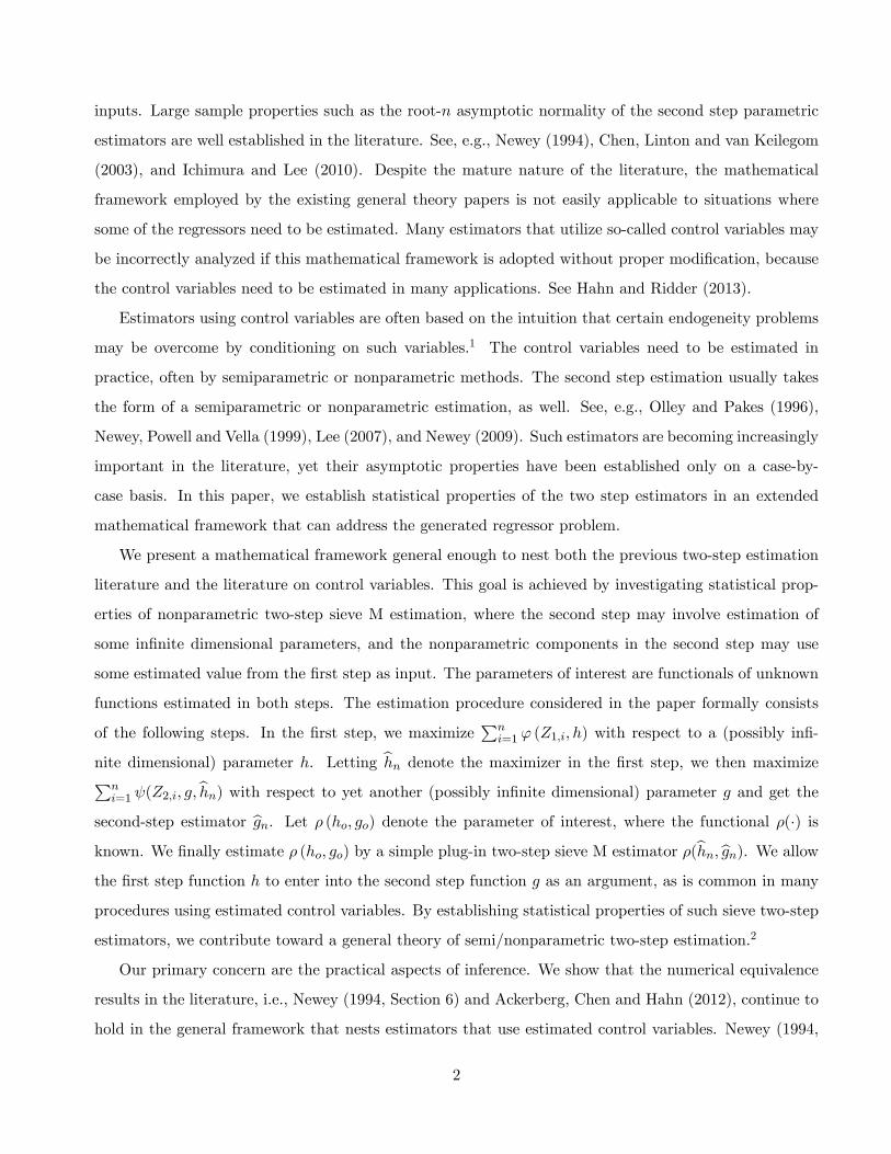
Figure 7.1. The Mean Square Errors of the Two-step Sieve M Estimators of mo and �o (DGP1)
Figure 1: 1. The left panel represents the MSEs of the two-step sieve estimator of mo for sample sizes n=100,250 and 500 respectively; 2. the right panel represents the MSEs of the two-step sieve estimator of �o for samplesizes n=100, 250 and 500 respectively; 3. L� and K� denote the numbers of the series terms which produce sieveestimator of mo with the smallest �nite sample MSE (in the left panel) or sieve estimator of �o with the smallest�nite sample MSE (in the left panel); 4. the dotted line represents the MSE of the two-step sieve M estimator withL = L� and K = K�; 5. the solid line represents the MSE of the two-step sieve M estimator with L and K selectedby 5-fold cross-validation.
26
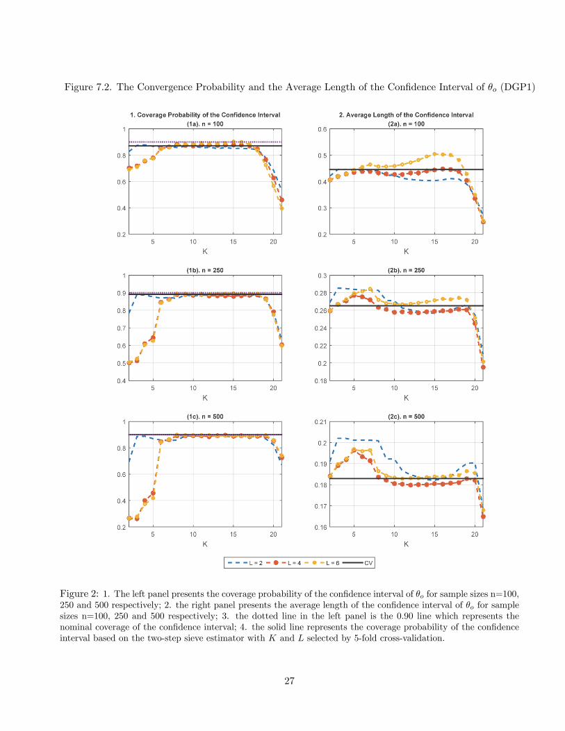
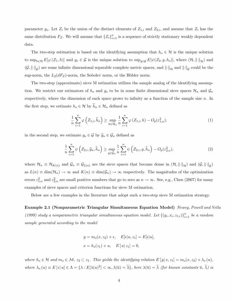
Figure 7.2. The Convergence Probability and the Average Length of the Con�dence Interval of �o (DGP1)
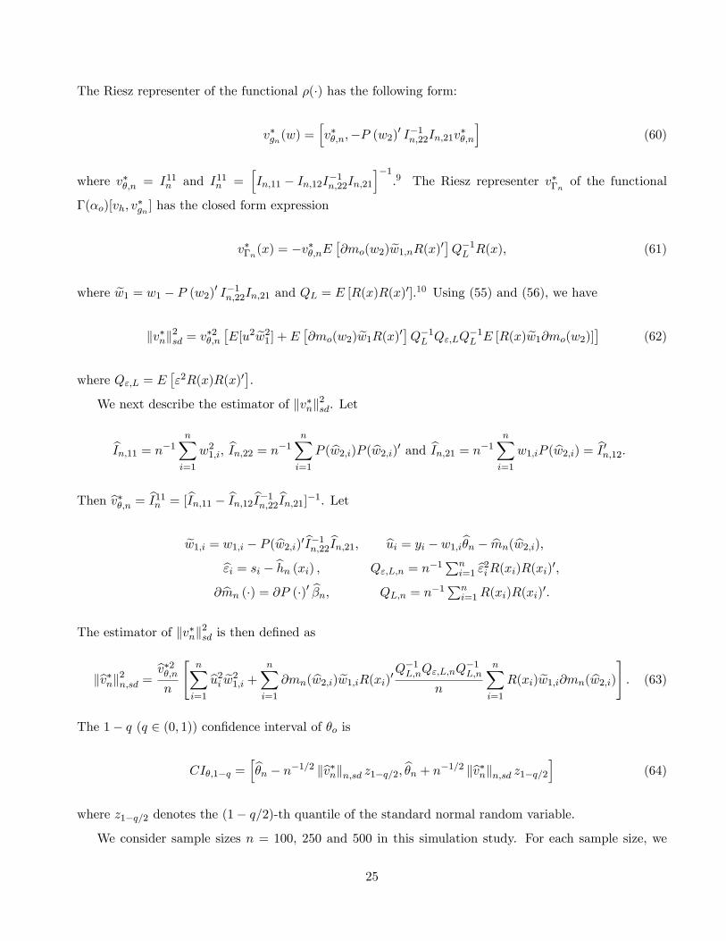
Figure 2: 1. The left panel presents the coverage probability of the con�dence interval of �o for sample sizes n=100,250 and 500 respectively; 2. the right panel presents the average length of the con�dence interval of �o for samplesizes n=100, 250 and 500 respectively; 3. the dotted line in the left panel is the 0.90 line which represents thenominal coverage of the con�dence interval; 4. the solid line represents the coverage probability of the con�denceinterval based on the two-step sieve estimator with K and L selected by 5-fold cross-validation.
27
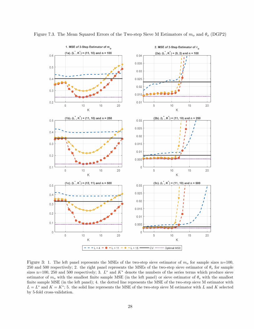
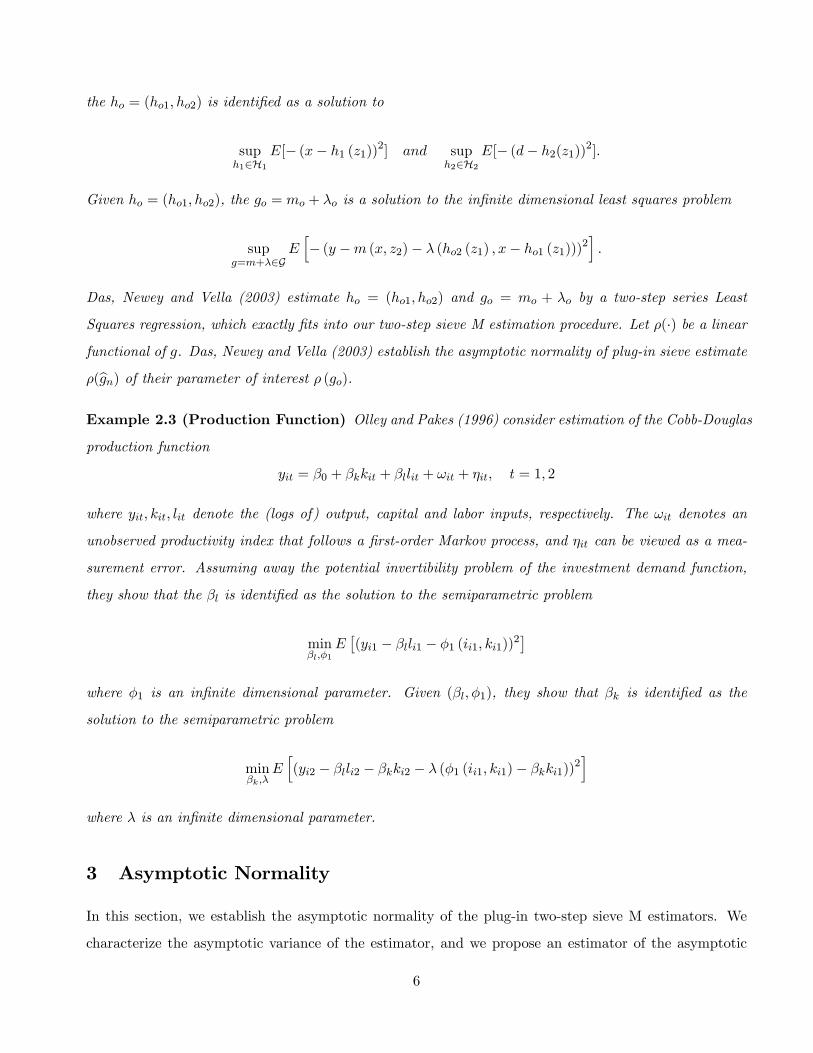
Figure 7.3. The Mean Squared Errors of the Two-step Sieve M Estimators of mo and �o (DGP2)
Figure 3: 1. The left panel represents the MSEs of the two-step sieve estimator of mo for sample sizes n=100,250 and 500 respectively; 2. the right panel represents the MSEs of the two-step sieve estimator of �o for samplesizes n=100, 250 and 500 respectively; 3. L� and K� denote the numbers of the series terms which produce sieveestimator of mo with the smallest �nite sample MSE (in the left panel) or sieve estimator of �o with the smallest�nite sample MSE (in the left panel); 4. the dotted line represents the MSE of the two-step sieve M estimator withL = L� and K = K�; 5. the solid line represents the MSE of the two-step sieve M estimator with L and K selectedby 5-fold cross-validation.
28

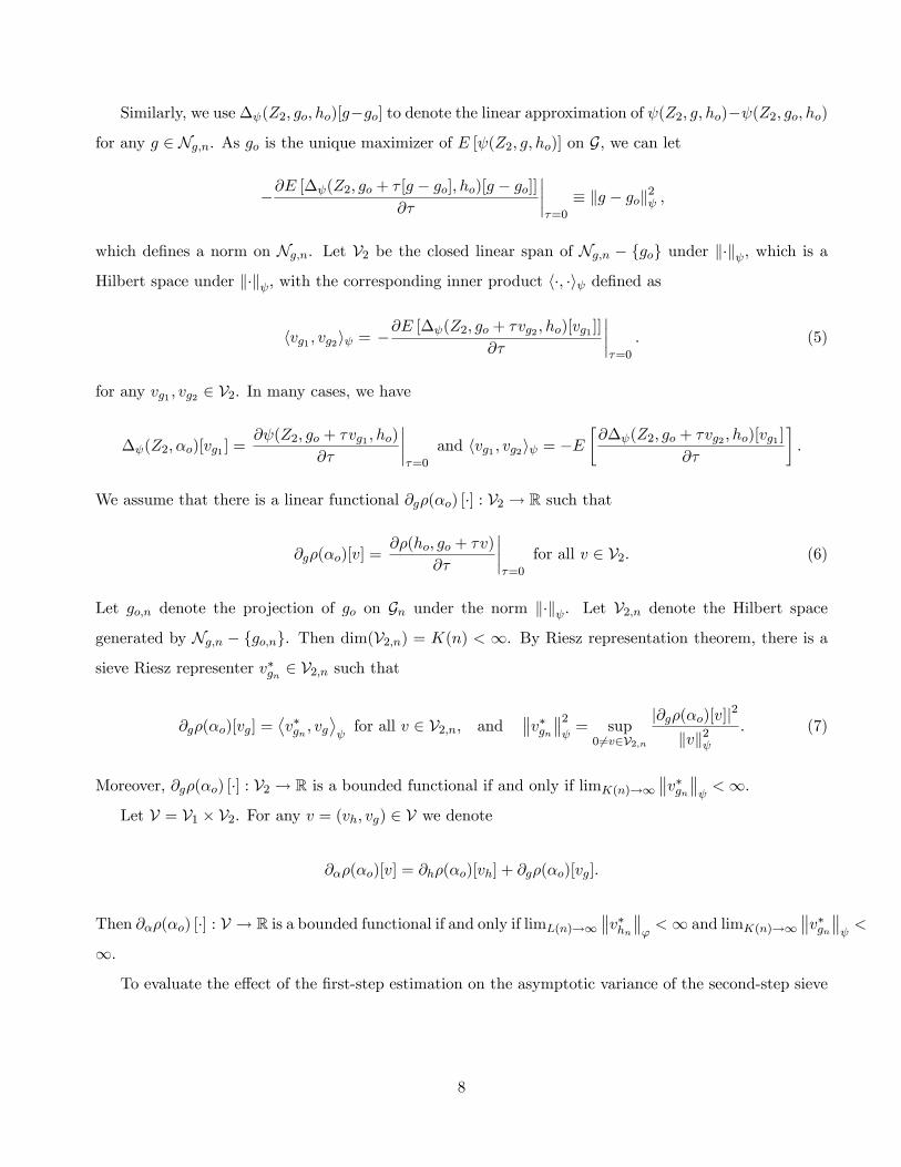
Figure 7.4. The Convergence Probability and the Average Length of the Con�dence Interval of �o (DGP2)
Figure 4: 1. The left panel presents the coverage probability of the con�dence interval of �o for sample sizes n=100,250 and 500 respectively; 2. the right panel presents the average length of the con�dence interval of �o for samplesizes n=100, 250 and 500 respectively; 3. the dotted line in the left panel is the 0.90 line which represents thenominal coverage of the con�dence interval; 4. the solid line represents the coverage probability of the con�denceinterval based on the two-step sieve estimator with K and L selected by 5-fold cross-validation.
29

generate 10000 simulated samples to evaluate the performances of the two-step sieve estimator and the
proposed inference procedure. For each simulated sample, we calculate the sieve estimator of (�o;mo), and
the 0.90 con�dence interval of �o for each combination of (L;K) where L = 2; : : : ; 16 and K = 2; : : : ; 21.
The simulation results are presented in Figures 7.1, 7.2, 7.3 and 7.4.
In Figure 7.1, we see that when the numbers of the series functions (L and K) are too small, the mean
square errors (MSEs) of the estimators of mo and �o are big.11 That is due to the large approximation
errors in the �rst-step and second-step nonparametric estimation when L and K are small. On the other
hand, the MSEs of the sieve estimators are also big when L and K are too large. That is because in this
case the stochastic estimation error in the two-step nonparametric estimation is big. The optimal L and
K which minimize the �nite sample MSE of the sieve estimator will balance the trade-o¤ between the
approximation error and the stochastic estimation error in the two-step nonparametric estimation. It is
interesting to see that the optimal L and K which minimize the MSE of the estimator of mo are smaller
than their counterparts which minimize the MSE of the estimator of �o (the only exception is the optimal
L when n = 100). With the growth of the sample size, the optimal L and K tend to increase. The black
solid line in Figure 7.1 represents the MSEs of the sieve estimators based on L and K selected by 5-fold
cross-validation.12 In the right panel of Figure 7.1, we see that as the sample size increases, the MSE of
the cross-validated estimator of �o approaches the optimal MSE (the dotted line) quickly. Moreover, the
solid line and the dotted line are almost identical when the sample size is 250. On the other hand, the
nonparametric J-fold cross-validated estimator usually enjoys the optimal convergence rate but it may
not necessarily be e¢ cient.13 In the left panel of Figure 7.1, it is interesting to see that the MSE of the
cross-validated sieve estimator of mo approaches the optimal value with the growth of the sample size.
The properties of the con�dence interval of �o in DGP1 are displayed in Figure 7.2. When L and
K are too small, the con�dence interval su¤ers large size distortion. The coverage probability in this
case becomes even worse with the growth of the sample size. This is because the con�dence interval is
miscentered due to the large approximation error which can not be reduced by increasing the sample
size. Meanwhile, the miscentered con�dence interval becomes narrower with larger sample sizes which
increases the size distortion for the con�dence interval with small L and K. On the other hand, the
coverage probability of the con�dence interval is far below 0.90 when L and K are too large. Two factors
may contribute to this phenomenon. First, the bias from the second order stochastic estimation error
becomes nontrivial when n is small, and L and K are large. This makes the proposed con�dence interval
miscentered in �nite samples. Second, the variance from the second order stochastic estimation error also
becomes nontrivial which means the con�dence interval in (64) is too narrow when L and K are too large.
30

The e¤ects of these two factors become small when the sample size is large, as we can see from Figure
7.2. The coverage probability of the con�dence interval based on the cross-validated sieve estimator is
slightly below the nominal level when n is small (i.e., n = 100), and it approaches the nominal level
quickly with a growing sample size. The right panel of Figure 7.2 shows good properties of the con�dence
interval based on the cross-validated sieve estimator. From the left panel of Figure 7.1, we see that when
L is small or large (i.e., L = 2 or 6), one can set K to be between 9 and 18 to achieve that that the
coverage probabilities of the resulting con�dence intervals are close to the nominal level. However, these
con�dence intervals tend to be much longer when compared with the con�dence interval based on the
cross-validated sieve estimator.
The simulation results under DGP2 are presented in Figure 7.3 and Figure 7.4. The properties of
the two-step sieve M estimator and the proposed con�dence interval are similar to what we found in
DGP1. We list some important di¤erences. First, when the unknown function estimated in the �rst-
step has unbounded support, the optimal L which produces a two-step M estimator with the smallest
MSE is much larger. Second, the ratio between the MSE of the cross-validated estimator of mo and the
optimal MSE does not seem to converge to 1 in all the sample sizes we considered. However, the MSE of
the cross-validated estimator of �o does approach the optimal value quickly as the sample size increases.
Third, when L is small (e.g., L = 4), the proposed con�dence interval over-covers the unknown parameter
�o and its length diverges with increasing K. Fourth, the coverage probability of the con�dence interval
based on the cross-validated sieve estimator is almost identical to the nominal level even when the sample
size is small (e.g., n = 100).
8 Conclusion
In this paper, we examined statistical properties of two-step sieve M estimation, where both the �rst and
second step models may involve in�nite dimensional parameters, and the nonparametric components in
the second step model may use the �rst-step unknown functions as arguments. Our theoretical results
expand the applicability of semi/nonparametric methods in estimation and inference of complicated
structural models. On a practical level, we established a generalization of the result of Ackerberg, Chen,
and Hahn (2012). We show that, even in a more complex semiparametric model with generated regressors,
one can implement a two-step linear sieve procedure as if it were a parametric procedure in the spirit of
Newey (1984) and Murphy and Topel (1985).
31
Notes
1See Chesher (2003), Altonji and Matzkin (2005), Blundell and Powell (2004, 2007), Florens, Heckman, Meghir and
Vytlacil (2008), and Imbens and Newey (2009), among others.2Outside of the sieve estimation framework, there are similar attempts for such a generalization. See, e.g., Ahn (1995),
Lewbel and Linton (2002), Mammen, Rothe and Schienle (2012, 2015) and the references therein. Unlike these papers, we
provide equivalence and robustness results, which are expected to be appealing to practitioners.3The derivation of these results in the general nonparametric nonlinear models, which are based on standard arguments,
can be found in the Supplemental Appendix of this paper.4 In some examples (see, e.g., the examples in Subsection 6.1 and Section 5), the two "score functions" �'(Z1;i; ho)[vh]
and � (Z2;i; �o)[vg] are orthogonal with each other for any vh and vg. Hence when the data is i.i.d., the sieve variance can
be more concisely written as kv�nk2sd = Eh���'(Z1;i; ho)[v�hn + v��n ]��2i+ E h��� (Z2;i; �o)[v�gn ]��2i.
5By combining the results of this paper with those of Chen, Liao and Sun (2014), one can show that analogous results
carry over to weakly dependent time series data.6Explicit characterization of bV� and bV�m is straightforward, and is omitted to keep the notation simple.7This is derived by applying Lemma C.6 in Appendix C.8Conjecture 2.1 in Li and Wooldridge (2002) is on the joint limiting distribution of b�n and b�n, where b�n is the �rst step
LS estimate. Although the weak convergence is only on b�n, we can de�ne the functional �(�) = �0(�0; �0)0 and derive the
asymptotic variance of (b�n; b�n).9The form of v�gn(�) in (60) is directly from (110) in Appendix C.10The form of v��n(�) in (61) is directly from (106) and (108) in Appendix C.11Let bmn;L;K(�) denote the second-step M-estimator of mo(�) based on the simulated sample with sample size n, and the
numbers of series functions L and K in the �rst-step and second step nonparametric estimations respectively. The empirical
MSE of bmn;L;K(�) is n�1Pni=1 jbmn;L;K(w2;i)�mo(w2;i)j2. The MSE of bmn;L;K(�) refers to the average of the empirical
MSEs of the 10000 simulated samples.12The J-fold cross-validation is described in Appendix A.13The cross-validated nonparametric estimator is called e¢ cient if the ratio of its MSE and the optimal MSE converges
to 1.
References
[1] Ackerberg, D., X. Chen, and J. Hahn (2012): �A Practical Asymptotic Variance Estimator for
Two-Step Semiparametric Estimators,�Review of Economics and Statistics, 94, 481-498.
[2] Altonji, J. and R. Matzkin (2005): �Cross Section and Panel Data Estimators for Nonseparable
Models With Endogenous Regressors,�Econometrica, 73, 1053-1102.
32

[3] Blundell, R., and J.L. Powell (2004): �Endogeneity in Semiparametric Binary Response Models,�
Review of Economic Studies 71, 655-679.
[4] Blundell, R., and J.L. Powell (2007): �Censored Regression Quantiles with Endogenous Regressors,�
Journal of Econometrics 141, 65-83.
[5] Chen, X. (2007): �Large Sample Sieve Estimation of Semi-Nonparametric Models,� In: James J.
Heckman and Edward E. Leamer, Editor(s), Handbook of Econometrics, 6B, Pages 5549-5632.
[6] Chen, X. and Z. Liao (2014): �Sieve M Inference of Irregular Parameters,�Journal of Econometrics,
182(1), 70-86
[7] Chen, X., Z. Liao and Y. Sun (2014): �Sieve Inference on Possibly Misspeci�ed Semi-nonparametric
Time Series Models,�Journal of Econometrics, 178(3), 639-658.
[8] Chen, X., O. Linton and I. van Keilegom (2003): �Estimation of Semiparametric Models when the
Criterion Function is not Smooth,�Econometrica, 71, 1591-1608.
[9] Chen, X. and X. Shen (1998): �Sieve Extremum Estimates for Weakly Dependent Data,�Econo-
metrica, 66, 289-314.
[10] Chesher, A. (2003): �Identi�cation in Nonseparable Models,�Econometrica, 71(5), 1405�14
[11] Das, M., W. Newey, and F. Vella (2003): �Nonparametric Estimation of Sample Selection Models,�
Review of Economic Studies, 70, 33-58.
[12] Florens, J., J. Heckman, C. Meghir and E. Vytlacil (2008): �Identi�cation of Treatment E¤ects Using
Control Functions in Models with Continuous, Endogenous Treatment and Heterogeneous E¤ects,�
Econometrica, 76, 1191-1206.
[13] Hahn, J., and G. Ridder (2013): �The Asymptotic Variance of Semi-parametric Estimators with
Generated Regressors,�Econometrica, 81, 315-340.
[14] Ichimura, H., and S. Lee (2010): �Characterization of the Asymptotic Distribution of Semiparametric
M estimators,�Journal of Econometrics, 159, 252-266.
[15] Imbens, G. and W. Newey (2009): �Identi�cation and Estimation of Triangular Simultaneous Equa-
tions Models Without Additivity,�Econometrica, 77, 1481-1512.
33
[16] Lee, S. (2007): �Endogeneity in quantile regression models: A Control function approach,�Journal
of Econometrics, 141, 1131-1158.
[17] Lewbel, A., and Linton, O. (2002): �Nonparametric Censored and Truncated Regression,�Econo-
metrica, 70, 765-779
[18] Li, Q. and M. Wooldridge (2002): �Semiparametric Estimation of Partially Linear Models for De-
pendent Data with Generated Regressors,�Econometric Theory, 18, 625-645.
[19] Mammen, E., C. Rothe and M. Schienle (2012): "Nonparametric Regression with Nonparametrically
Generated Covariates," Annals of Statistics, 40, 1132-1170.
[20] Mammen, E., C. Rothe and M. Schienle (2015): "Semiparametric Estimation with Generated Co-
variates," Econometric Theory, forthcoming.
[21] Murphy, K. and R. Topel (1985): �Estimation and Inference in Two-Step Econometric Models,�
Journal of Business and Economic Statistics, 3, 370-379.
[22] Newey, W. (1984): �A Method of Moments Interpretation of Sequential Estimators,� Economics
Letters, 14, 201-206.
[23] Newey, W. (1994): �The Asymptotic Variance of Semiparametric Estimators,�Econometrica, 62,
1349-1382.
[24] Newey, W., J. Powell, and F. Vella (1999): �Nonparametric Estimation of Triangular Simultaneous
Equations Models,�Econometrica, 67, 565-603.
[25] Newey, W. (2009): �Two-Step Series Estimation of Sample Selection Models,�Econometrics Journal,
12, S217�S229.
[26] Olley, G. and A. Pakes (1996): �The Dynamics of Productivity in the Telecommunications Equip-
ment Industry,�Econometrica, 64, 1263-1297.
[27] Shen, X. (1997): �On Methods of Sieves and Penalization�, Annals of Statistics, 25, 2555-2591.
[28] Wooldridge, J.M. (2002): Econometric Analysis of Cross Section and Panel Data, Cambridge: MIT
Press.
34

Appendix
A A Cross-Validation Method for Selecting the Tuning Parameters
In this appendix, we describe the cross-validation procedure used for selecting the numbers of series termsin the two-step sieve M estimation. We �rst introduce some notation. For j = 1; : : : ; J (where J is a �nitepositive integer), let Ij be a subset of I = f1; 2; : : : ; ng such that I1 [ � � � [ IJ = I and Ij1 \ Ij2 = ? forany j1 6= j2. Let nj be the number of elements in Ij for j = 1; : : : ; J . Let Ln and Kn be the user speci�edsets of candidate values of L and K for the two-step M estimation. For example, in the simulation studyof this paper, we set Ln = f2; : : : ; 15g and Kn = f2; : : : ; 21g.
For each j = 1; : : : ; J and each L 2 Ln, we calculate the �rst-step M estimator bhj;L asn�1j
Xi2Ij
'(Z1;i;bhj;L) � suph2HL
n�1jXi2Ij
' (Z1;i; h)�Op("21;nj ); (65)
where HL is the sieve space generated by L basis functions. Given bhj;L, we calculate the second-step Mestimator bgj;K as
n�1jXi2Ij
(Z2;i; bgj;K ;bhj;L) � supg2GK
1
n
nXi=1
(Z2;i; g;bhj;L)�Op("22;nj ); (66)
for each j = 1; : : : ; J , each L 2 Ln and each K 2 Kn, where GK is the sieve space generated by Kbasis functions. The numbers of series terms L� and K� are then selected by the following minimizationproblem:
(L�;K�) = argminL2Ln; K2Kn
J�1JXj=1
24(n� nj)�1Xi2Icj
(Z2;i; bgj;K ;bhj;L)35 (67)
where Icj denotes the complement of Ij for j = 1; : : : ; J . The cross-validated two-step M estimator is thencalculated by plugging (L�;K�) into the estimation problems (1) and (2) in Section 2.
B Proof of Results in Section 3
Proof of Theorem 3.1. Recall that g� = g � �nu�gn , where �n = o(n�
12 ) and u�gn � v�gn kv
�nk�1sd . By
Assumption 3.3.(iii), �n���12;n = o (1) and the triangle inequality, we have
jjbg�n � gojj � jjbgn � gojj + �njju�gn jj = Op(��2;n) (68)
which implies that bg�n 2 Ng;n wpa1.
35

By the de�nition of bgn, we have�Op
�"22;n
�� 1
n
nXi=1
�Z2;i; bgn;bhn�� 1
n
nXi=1
�Z2;i; bg�n;bhn�
= �n
n (Z2; bgn;bhn)� (Z2; bg�n;bhn) + � (Z2; bgn;bhn)[��nu�gn ]o
+ �n
n� (Z2; go; ho)[��nu�gn ]�� (Z2; bgn;bhn)[��nu�gn ]o
� �n�� (Z2; go; ho)[��nu�gn ]
+hK (bgn;bhn)�K (bg�n;bhn)i : (69)
By Assumption 3.2.(i), we have
�n
n (Z2; bgn;bhn)� (Z2; bg�n;bhn) + � (Z2; bgn;bhn)[��nu�gn ]o = Op(�
2n) (70)
and �nn� (Z2; go; ho)[u
�gn ]�� (Z2; bgn;bhn)[u�gn ]o = Op(�n): (71)
Note that �(�o)[�; �] is a bilinear functional. Using (68), Assumption 3.2.(ii) and Assumption 3.3.(iii), wededuce that
K (bgn;bhn)�K (bg�n;bhn)= ��n�(�o)[bhn � ho; u�gn ] + jjbg�n � gojj2 � jjbgn � gojj2 2
+ op��2n�
= h��nu��n ;bhn � hoi' + �2njju�gn jj2 2
+ h��nu�gn ; bgn � goi + op ��2n�= h��nu��n ;bhn � hoi' + h��nu�gn ; bgn � goi +Op ��2n� : (72)
From "2;n = O (�n), (69), (70), (71) and (72), we get
�Op�"2n�� ��n�n
�� (Z2; go; ho)[u
�gn ]� �nhu��n ;bhn � hoi' � �nhu�gn ; bgn � goi :
Dividing by �n, we obtain���bgn � go; u�gn� � hbhn � ho; u��ni' � �n �� (Z2; go; ho)[u�gn ]��� = Op(�n): (73)
By de�nition, go;n is the projection of go on V2;n under the semi-norm k�k . Hence there is hgo;n �go; u
�gni = 0 and
hbgn � go; u�gni = hbgn � go;n; u�gni : (74)
From (73), (74) and �n = o(n�12 ), we get���hbgn � go;n; u�gni � hbhn � ho; u��ni' � �n �� (Z2; go; ho)[u
�gn ]��� = op(n
� 12 ): (75)
36

By Assumption 3.1.(i)-(iii) and the Riesz representation theorem,
pn�(bhn; bgn)� �(ho;n; go;n)
kv�nksd=pn@�(�o)@h [bhn � ho;n] + @�(�o)
@h [bgn � go;n]kv�nksd
+pn�(bhn; bgn)� �(ho; go)� @�(�o)
@h [bhn � ho]� @�(�o)@g [bgn � go]
kv�nksd
�pn�(ho;n; go;n)� �(ho; go)� @�(�o)
@h [ho;n � ho]� @�(�o)@g [go;n � go]
kv�nksd=pnhhbhn � ho;n; u�hni' + hbgn � go;n; u�gni i+ op(1): (76)
By de�nition, ho;n is the projection of ho on V1;n under the semi-norm k�k'. Hence there is hho �ho;n; u
�hni' = 0 and
hbhn � ho;n; u�hni' = hbhn � ho; u�hni': (77)
From the results in (76) and (77), we get
pnh�(bhn; bgn)� �(ho;n; go;n)i
kv�nksd=pnhhbhn � ho; u�hni' + hbgn � go;n; u�gni i+ op(1)
which, together with (75) and Assumption 3.3.(i), implies that
pnh�(bhn; bgn)� �(ho;n; go;n)i
kv�nksd=pnhhbhn � ho; u�hn + u��ni' + �n �� (Z2; go; ho)[u
�gn ]i+ op(1)
= n�12
nXi=1
��'(Z1;i; ho)[u
�hn + u
��n ] + � (Z2;i; go; ho)[u
�gn ]+ op(1): (78)
Now the result in (14) follows immediately by (78) and Assumption 3.3.(ii).From Assumption 3.1, we get
�����(ho;n; go;n)� �(ho; go)kv�nksd
���� ��������(ho;n; go;n)� �(ho; go)�
@�(�o)@h [ho;n � ho]� @�(�o)
@g [go;n � go]kv�nksd
������+
1
kv�nksd
�����@�(�o)@h[ho;n � ho]
����+ ����@�(�o)@h[go;n � go]
�����= o(n�1=2); (79)
which combined with (14) immediately implies (15).
37

C Proof of Results in Section 4 and Section 6
Lemma C.1 Under Assumption 4.1, the empirical Riesz representer bv�gn satis�es: v�gn �1 bv�gn � v�gn = op(1): (80)
Proof. The proof follows the same arguments in the proof of Lemma 5.1 in Chen, Liao and Sun (2014)and hence is omitted.
Lemma C.2 Under Assumption 4.2, the empirical Riesz representers bv�hn and bv��n satisfy: v�hn �1' bv�hn � v�hn ' = op(1) and v��n �1' bv��n � v��n ' = op(1): (81)
Proof. The proof follows the same arguments in the proof of Lemma 5.1 in Chen, Liao and Sun (2014)and hence is omitted.
Lemma C.3 Under Assumption 4.3, we have:(i) sup
h2Nh;n;vh2W1;n
��n�1Pni=1�
2'(Z1;i; h)[vh]� E
��2'(Z1; ho)[vh]
��� = op(1);
(ii) sup�2Nn;vg2W2;n
���n�1Pni=1�
2 (Z2;i; �)[vg]� E
h�2 (Z2; �o)[vg]
i��� = op(1);
(iii) sup�2Nn;vh2W1;n;vg2W2;n
��n�1Pni=1�'(Z1;i; h)[vh]� (Z2;i; �)[vg]� E [�'(Z1; ho)[vh]� (Z2; �o)[vg]]
�� =op(1):
Proof of Lemma C.3. (i) By the triangle inequality, Hölder inequality, Assumption 4.3.(i) and (iv), wehave
suph2Nh;n;vh2W1;n
����� 1nnXi=1
�2'(Z1;i; h)[vh]� E��2'(Z1; ho)[vh]
������� sup
h2Nh;n;vh2W1;n
���n ��2'(Z1; h)[vh]��+ suph2Nh;n;vh2W1;n
��E ��2'(Z1; h)[vh]��2'(Z1; ho)[vh]���� op(1) + sup
h2Nh;n;vh2W1;n
k�'(Z1; h)[vh]��'(Z1; ho)[vh]k22
+ 2 suph2Nh;n;vh2W1;n
k�'(Z1; h)[vh]��'(Z1; ho)[vh]k2 k�'(Z1; ho)[vh]k2
= op(1)
which shows the �rst result.(ii) The second result can be proved using the same arguments in the proof of the �rst result, but
replacing Assumption 4.3.(i) with Assumption 4.3.(ii).
38

(iii) By the triangle inequality, we have
jE [�'(Z1; h)[vh]� (Z2; �)[vg]��'(Z1; ho)[vh]� (Z2; �o)[vg]]j
� jE [(�'(Z1; h)[vh]��'(Z1; ho)[vh]) (� (Z2; �)[vg]�� (Z2; �o)[vg])]j
+ jE [(�'(Z1; h)[vh]��'(Z1; ho)[vh])� (Z2; �o)[vg]]j
+ jE [�'(Z1; ho)[vh] (� (Z2; �)[vg]�� (Z2; �o)[vg])]j (82)
for any � 2 Nn, vh 2 W1;n and vg 2 W2;n. Using Hölder inequality, Assumption 4.3.(i) and (ii), we have
sup�2Nn;vh2W1;n;vg2W2;n
jE [(�'(Z1; h)[vh]��'(Z1; ho)[vh]) (� (Z2; �)[vg]�� (Z2; �o)[vg])]j
� sup�2Nn;vh2W1;n;vg2W2;n
k�'(Z1; h)[vh]��'(Z1; ho)[vh]k2 k� (Z2; �)[vg]�� (Z2; �o)[vg]k2 = o(1):
(83)
Similarly by Assumption 4.3.(i), (ii) and (iv), we have
suph2Nh;n;vh2W1;n;vg2W2;n
k�'(Z1; h)[vh]��'(Z1; ho)[vh]k2 k� (Z2; �o)[vg]k2 = o(1) (84)
andsup
�2Nn;vh2W1;n;vg2W2;n
k� (Z2; �)[vg]�� (Z2; �o)[vg]k2 k�'(Z1; ho)[vh]k2 = o(1): (85)
Now the claimed result follows immediately from Assumption 4.3.(iii), (82), (83), (84) and (85).
Proof of Theorem 4.1. Let c denote some generic �nite positive constant. As the data are i.i.d., byde�nition, we have
kv�nk2sd = Var
hn�
12
Xn
i=1
��'(Z1;i; ho)[v
�hn + v
��n ] + � (Z2;i; �o)[v
�gn ]�i
= Eh���'(Z1;i; ho)[v
�hn + v
��n ] + � (Z2;i; �o)[v
�gn ]��2i
= �'(Z1;i; ho)[v
�hn + v
��n ] + � (Z2;i; �o)[v
�gn ] 22: (86)
By the triangle inequality,
kbv�n � v�nksdkv�nksd
� �'(Z1; ho)[bv�hn � v�hn ] 2 + �'(Z1; ho)[bv��n � v��n ] 2 + � (Z2; �o)[bv�gn � v�gn ] 2
kv�nksd: (87)
39

Using (86), Assumption 4.3.(iv) and the result in (80), we have
� (Z2; �o)[bv�gn � v�gn ] 2kv�nksd
=
v�gn kv�nksd
bv�gn � v�gn v�gn � (Z2; �o)
" bv�gn � v�gn bv�gn � v�gn #
2
and because�bv�gn � v�gn�� bv�gn � v�gn 2 Wgn , we have
� (Z2; �o)[bv�gn � v�gn ] 2kv�nksd
�
v�gn kv�nksd
bv�gn � v�gn v�gn supvg2Wgn
k� (Z2; �o)[vg]k2 = op(1): (88)
Similarly, we have �'(Z1; ho)[bv�hn � v�hn ] 2 + �'(Z1; ho)[bv��n � v��n ] 2kv�nksd
= op(1)
which together with (87) and (88) implies that
kv�nk�1sd kbv�n � v�nksd = op(1): (89)
Using (89) and the triangle inequality, we get
op(1) =kbv�n � v�nksdkv�nksd
�����kbv�nksdkv�nksd
� 1���� =
����� kbv�nksdkbv�nkn;sd kbv�nkn;sdkv�nksd
� 1�����
=���kbv�nk�1n;sd kbv�nksd �kv�nk�1sd kbv�nkn;sd � 1�+ �kbv�nk�1n;sd kbv�nksd � 1���� : (90)
We next show that kbv�nk�1n;sd kbv�nksd � 1 = op(1). For this purpose, we �rst note that
bv�hn + bv��n 'kbv�nksd �
v�hn + v��n ' + bv�hn � v�hn ' + bv��n � v��n 'kbv�nksd
�
v�hn ' + v��n ' + v�hn ' kbv�hn�v�hnk'kv�hnk'+ v��n ' kbv��n�v��nk'kv��nk'
kbv�nksd=
v�hn 'kbv�nksd
1 +
bv�hn � v�hn ' v�hn '!+
v��n 'kbv�nksd
1 +
bv��n � v��n ' v��n '!
=kv�nksdkbv�nksd
" v�hn 'kv�nksd
(1 + op(1)) +
v��n 'kv�nksd
(1 + op(1))
#
=kv�nksdkbv�nksdOp(1) =
�1
kbv�nksd = kv�nksd � 1�Op(1) +Op(1) = Op(1) (91)
40

where the �rst two inequalities are by the triangle inequality, the second equality is by (81), the thirdequality is by (86) and (25), and the last equality is by the �rst inequality in (90). Similarly, we can showthat bv�gn kbv�nk�1sd = Op(1): (92)
By the triangle inequality, we get
�����kbv�nk2n;sd � kbv�nk2sdkbv�nk2sd
����� =�������1n
Pni=1
h�'(Z1;i;bhn)[bv�hn + bv��n ] + � (Z2;i; b�n)[bv�gn ]i2
kbv�nk2sd�EZ
h���'(Z1; ho)[bv�hn + bv��n ] + � (Z2; �o)[bv�gn ]��2ikbv�nk2sd
������� jI1;nj+ jI2;nj+ 2 jI3;nj (93)
where EZ [�] denotes the expectation taking with respect to the distribution of Z (EZ1 [�] and EZ2 [�] aresimilarly de�ned),
I1;n =1n
Pni=1�
2'(Z1;i;
bhn)[bv�hn + bv��n ]� EZ1 ��2'(Z1; ho)[bv�hn + bv��n ]�kbv�nk2sd ;
I2;n =
1n
Pni=1�
2 (Z2;i; b�n)[bv�gn ]� EZ2 h�2 (Z2; �o)[bv�gn ]i
kbv�nk2sdand
I3;n =1n
Pni=1�'(Z1;i;bhn)[bv�hn + bv��n ]� (Z2;i; b�n)[bv�gn ]
kbv�nk2sd�EZ��'(Z1; ho)[bv�hn + bv��n ]� (Z2; �o)[bv�gn ]�
kbv�nk2sd :
By Lemma C.3.(i) and (91), we have
jI1;nj =
bv�hn + bv��n 2'kbv�nk2sd
��� 1nPni=1�
2'(Z1;i;
bhn)[bv�hn + bv��n ]� EZ1 ��2'(Z1; ho)[bv�hn + bv��n ]���� bv�hn + bv��n 2'� Op(1) sup
h2Nh;n;vh2W1;n
����� 1nnXi=1
�2'(Z1;i; h)[vh]� EZ1��2'(Z1; ho)[vh]
������ = op(1): (94)
41

Similarly, by Lemma C.3.(ii) and (92), we have
jI2;nj =
bv�gn 2 kbv�nk2sd
��� 1nPni=1�
2 (Z2;i; b�n)[bv�gn ]� EZ2 h�2 (Z2; �o)[bv�gn ]i��� bv�gn 2 = op(1): (95)
For the last term I3;n, note that
jI3;nj �
bv�hn + bv��n ' bv�gn kbv�nk2sd
� sup�2Nn;vg2W2;n;vh2W1;n
������ n�1Pn
i=1�'(Z1;i; h)[vh]� (Z2;i; �)[vg]
�EZ [�'(Z1; h)[vh]� (Z2; �)[vg]]
������=
bv�hn + bv��n ' bv�gn kbv�nk2sd op(1) = op(1); (96)
where the �rst equality is by Lemma C.3.(iii), the last equality is by (91) and (92).From the results in (93), (94), (95) and (96), we deduce that�����kbv�nk
2n;sd � kbv�nk2sdkbv�nk2sd
����� = op(1): (97)
It is clear that (90) and (97) imply that���kbv�nkn;sd = kv�nksd � 1��� = op(1), which �nishes the proof.
We divide the proof of Proposition 6.1 into establishing several lemmas. We start with an explicitcharacterization of kv�nk
2sd when the data are i.i.d. and when both h and g are real-valued functions for
the sake of simpli�ed notation.Let Hn =
�h(�) = R(�)0 L : L 2 RL
be a sieve space for ho(�) in the �rst step, where R(�) is de�ned
in Section 6. Let Gn = fg(�) = P (�)0�g : �g 2 RKg be the sieve space for go(�) in the second step, whereP (�) is de�ned in Section 6. De�ne
R'(ho)[vh1 ; vh2 ] � hvh1 ; vh2i' and R (�o)[vg1 ; vg2 ] � hvg1 ; vg2i (98)
for any vh1 ; vh2 2 V1 and vg1 ; vg2 2 V2. Finally, we let �'(R) � �'(Z1; ho)[R] be L � 1 and � (P ) �� (Z2; �o)[P ] be K � 1, and
�(P; P ) �
0@ �'(R)�0'(R) �'(R)�
0 (P )
� (P )�0'(R) � (P )�
0 (P )
1A be (L+K)� (L+K):
42

Recall that for i.i.d. data, we have
kv�nk2sd = E
h���'(Z1; ho)[v�hn + v
��n ] + � (Z2; �o)[v
�gn ]��2i :
Lemma C.4 Let @h�(�o)[R] and @g�(�o)[P ] denote L�1 and K�1 vectors with the j-th elements being@h�(�o)[rj ] and @g�(�o)[pj ] respectively. Let R'(ho)[R;R] and R (�o)[P ; P ] be L�L and K�K matriceswith the (a; b)-th elements being R'(ho)[ra; rb] and R (�o)[pa; pb] respectively. Let �(�o)
�R; v�gn
�be L�1
vector with the j-th element being �(�o)�rj ; v
�gn
�and � (�o)
�R;P
�be L � K matrix with the (a; b)-th
element being � (�o) [ra; pb]. We then have
v�hn(�) = R(�)0 [R'(ho)[R;R]]�1 @h�(�o)[R] � R(�)0��hn ; (99)
v�gn(�) = P (�)0�R (�o)[P ; P ]
��1@g�(�o)[P 2] � P (�)0��gn ; (100)
v��n(�) = R(�)0 [R'(ho)[R;R]]�1 �(�o)�R; v�gn
�� R(�)0���n (101)
and���n = [R'(ho)[R;R]]
�1 � (�o)�R;P
���gn : (102)
Proof. Let ��hn be such that v�hn= R(�)0��hn . Note that we have
@h�(�o) [rj ] =rj ; v
�hn
�'= R'(ho)
�rj ; R
0(�)��hn�= R'(ho) [rj ; R]
0 ��hn
for all j. It follows that @h�(�o) [R] = R'(ho) [R;R]��hnand hence ��hn = (R'(ho) [R;R])
�1 @h�(�o) [R],which proves (99). We can prove (100) and (101) similarly, and the details are omitted. As for (102), byde�nition we have
�(�o)�R; v�gn
�= � (�o)
�R;P
���gn :
Using (101), we obtain
���n = [R'(ho)[R;R]]�1 �(�o)
�R; v�gn
�= [R'(ho)[R;R]]
�1 � (�o)�R;P
���gn :
Lemma C.5
kv�nk2sd =
���0hn ; ��0gn
�0@ IL 0
A0n IK
1AE [�(P; P )]
0@ IL An
0 IK
1A0@ ��hn
��gn
1A : (103)
whereAn � [R'(ho)[R;R]]�1 � (�o)
�R;P
�is L�K: (104)
43

Proof. Because kv�nk2sd = Var
��'(Z1;i; ho)[v
�hn+ v��n ] + � (Z2;i; �o)[v
�gn ]�, it follows that
kv�nk2sd =
���0hn + �
�0�n; ��0gn
�E [�(P; P )]
���0hn + �
�0�n; ��0gn
�0: (105)
Combining with (102) in Lemma C.4, we then obtain
v��n(�) = R(�)0An��gn (106)
Finally, combining (105) and (106), we obtain the desired conclusion.
In the rest of this appendix, we provide explicit expressions of sieve variances for the two functionalconsidered in Section 4 when go = (�o;mo(�)). The �rst functional is �(�) = �0� for some � 6= 0 in Rd� ,where � = (h(�); g(�)) = (h(�); �;m(�)).
Lemma C.6 For �(�) = �0�, we have
v��;n 2sd = �0�I(1)��;n;�I
(1)��;nI�m;nI
�1mm;n
�E�Vg;iV
0g;i
� �I(1)��;n;�I
(1)��;nI�m;nI
�1mm;n
�0�; (107)
where Vg;i = (�(�o)�R;P
�)0 [R'(ho)[R;R]]
�1�'(Z1;i; ho)[R] + � (Z2;i; �o)[P ].
Proof. In this case, it is clear that we have vg(�) = (v�; vm(�)), where vm(�) = P (�)0�K . Hence for anyvg 2 Vgn with vg = (v�; vm(�)) and vm(�) = P 02(�)�K , we can write
hvg; vgi = (v0�; �0K)R (�o)[P ; P ](v0�; �0K)0:
By de�nition, we have
R (�o)[P ; P ] =
0@ I��;n I�m;n
Im�;n Imm;n
1Awhere I��;n and Imm;n are d� � d� and L� L matrices respectively.
Because @g�(�o)�P�= (�0;00L)
0, we can use (100) in Lemma C.4 along with the partitioned inverseformula, and conclude
��gn � (����n�0; (��K)
0)0 =��0I
(1)��;n;��
0I(1)��;nI�m;nI
�1mm;n
�0; (108)
where I(1)��;n =�I��;n � I�m;nI�1mm;nIm�;n
��1. Likewise, we can conclude that ��hn = 0. We therefore obtain���0hn ��0gn
�0@ IL 0
A0n IK
1A0@ �'(R)
� (P )
1A = ��0gnA0n�'(R) + �
�0gn� (P ) = ��0gnVg: (109)
The conclusion follows by combining (108) and (109) with Lemma C.5.
44

From (108), we see that the Riesz representer v�g(�) of the functional �(�o) = �0�o takes the followingform:
v�g(�) =��0I
(1)��;n;��
0I(1)��;nI�m;nI
�1mm;n
�0P (�) =
��0I
(1)��;n1d� ;��
0I(1)��;nI�m;nI
�1mm;nP (�)
�: (110)
Lemma C.7 For �(�) = �(mo), we have
v�m;n 2sd = @�(mo)[P ]0��I(1)mm;nIm�;nI�1��;n; I
(1)mm;n
�E�Vg;iV
0g;i
� ��I(1)mm;nIm�;nI�1��;n; I
(1)mm;n
�0@�(mo)[P ]:
(111)
Proof. Because @g�(�o)�P 2�=�00d� ; @�(mo)[P ]
0�0, we obtain
��gn =�R (�o)[P 2; P 2]
��1 �00d� ; @�(mo)[P ]
0�0 = ��@�(mo)[P ]0I(1)mm;nIm�;nI
�1��;n; @�(mo)[P ]
0I(1)mm;n
�0so we have �
��gn�0= @�(mo)[P ]
0��I(1)mm;nIm�;nI�1��;n; I
(1)mm;n
�Likewise, we can conclude that ��hn = 0. We therefore obtain
���0hn ��0gn
�0@ Ik1(n) 0
A0n Ik2(n)
1A0@ �'(P1)
� (P 2)
1A = ��0gnA0n�'(P1) + �
�0gn� (P 2) = ��0gnVg:
As in the previous lemma, the conclusion follows by using Lemma C.5.
Proof of Proposition 6.1. Recalling that our estimator of the asymptotic variance is nothing but the
sample analog of v��;n 2
sd, we can obtain from Lemma C.6 that
bv��;n 2sd = �b��0�n ;�b��0�n bI�m;nbI�1mm;n�Pn
i=1bVg;i bV 0g;in
�b��0�n ;�b��0�n bI�m;nbI�1mm;n�0 ; bv�m;n 2sd = ��b��0mn bIm�;nbI�1��;n; b��0mn�Pn
i=1bVg;i bV 0g;in
��b��0mn bIm�;nbI�1��;n; b��0mn�0 ;
which proves Proposition 6.1.
Proof of Theorem 6.2. By de�nition, we have
�n(b�n) �R;P � = n�1nXi=1
@2 (Z2;i; bg(�);bh(�))@ L@�0g
;
n�1nXi=1
r (Z2;i; b�n)[P ; P ] = n�1nXi=1
@2 �Z2;i; bg(�);bh(�)�@�g@�0g
;
�'(Z1;bhn)[R] = @'(Z1;bhn(�))@ L
and � (Z2; b�n)[P ] = @ (Z2; bg(�);bh(�))@�g
:
45

It follows that bI ;�� = bI��;n, etc., bV22 = n�1Pn
i=1bVg;i bV 0g;i, from which we obtain the conclusion.
D Proof of Results in Section 5
In this appendix, we provide the su¢ cient conditions of Theorem 5.1. For any column vector a, let kakdenote its `2-norm. For any square matrix A, the operator norm is denoted by jjAjj. Let khkH = khk2and kgkG = kgk2. Let C denote some generic �nite constant larger than 1. By de�nition, go;n and ho;nare the projections of go and ho under the L2-norm respectively. Let X denote the support of x. For easeof notations, we omit the dependence of L(n) and K(n) on n, and write L(n) = L and K(n) = K.
Assumption D.1 (i) The data fyi; xi; signi=1 is i.i.d.; (ii) E�"4i��xi� < C and E["2i
��xi] > C�1; (iii)there exist �h > 0 and o;L 2 RL such that
kho;L � hok1 = O(L��h)
where ho;L (�) � R (�)0 o;L; (iv) the eigenvalues of QL are between C�1 and C for all L; (v) there existsa nondecreasing sequence �L such that supx2X kR(x)k � �L.
We assume that the support of "i is E = [a; b], where a, b are �nite constants. De�ne E� = [a��; b+�]for some small � > 0. For d a nonnegative integer, let jgjd = maxj� j�d sup"2E j@�g(")j for any g 2 G.
Assumption D.2 (i) E[u4i�� "i] < C and E[u2i
�� "i] > C�1; (ii) go(") is twice continuously di¤erentiable;(iii) there exist �g > 0 and �o;K 2 RK such that
jgo;K � gojd = O(K��g)
where go;K (�) = P (�)0 �o;K and d = 1; (iv) the eigenvalues of QK are between C�1 and C for all K; (v)for j = 0; 1; 2, there exists a nondecreasing sequence �j;K such that sup"2E�
@jP (") � �j;K .
Assumptions D.1 and D.2 impose restrictions on the moments of the error terms u and ", and thesmoothness of unknown functions ho and go. Let �j;K = sup"2E�
@jP (")0�o;K for j = 1; 2. UnderAssumptions D.1 and D.2, and restrictions on the number of sieve basis functions in Assumption D.4below, we show in Lemma 1.1 of the Supplemental Appendix that
jjbhn � hojj = Op(��h;n) and kbgn � gok = Op(�
�2;n)
where ��h;n = L1=2n�1=2+L��h and ��2;n = K1=2n�1=2+K��g + �1;K��h;n. Let �2;n = ��2;n log(log(n)), then
we have bgn 2 Ng;n wpa1 where Ng;n = fg 2 Gn : kg � gok2 � �2;ng.The sequence �1;K e¤ects the rate of convergence of bgn derived in Lemma 1.1 of the Supplemental
Appendix. When the unknown function go(�) is well de�ned and is continuously di¤erentiable in theextended support E�, and �o;K satis�es
maxjjj�2
sup"2E�
��@jP (")0�o;K � @jgo(")�� = O(K��g); (112)
46
then we have�j;K � sup
"2E�
��@jP (")0�o;K � @jgo(")��+ sup"2E�
��@jgo(")�� = O(1): (113)
Let !min(QK) denote the smallest eigenvalue of QK . Then by the Cauchy inequality and AssumptionsD.2.(ii)-(v),
�j;K � sup"2E�
@jP (") k�o;Kk � sup"2E�
@jP (") !�1min(QK) �kgo;K � gok2 + kgok2� � C�j;K ; (114)
which provides a upper bound for �j;K when go(�) does not satisfy the extended support condition (113).
Assumption D.3 (i) jjv�gn jj2 � C for all n; (ii) the functional �(�) satis�es
supg2Ng;n
�����(g)� �(go)� @�(go)[g � go]kv�nksd
���� = o(n�1=2);
(iii)���kv�nk�1sd @�(go)[go;n � go]��� = o(n�1=2); (iv) supg2Ng;n k@�(g)[P ]� @�(go)[P ]k = o(1).
Assumption D.3.(i) requires that the L2-norm of the Riesz representer v�gn is uniformly bounded frombelow by some �xed constant. This condition together with the condition E[u2i
�� "i] > C�1 in AssumptionD.2.(i) imply that the sieve variance is bounded away from zero. Assumptions D.3.(ii)-(iv) imposesconditions on the functional �(�). These conditions can be easily veri�ed when the functional �(�) islinear.
Assumption D.4 The following conditions hold:(i) n�1=2(K + L)1=2(�0;K + �L)(log(n))
1=2 = o(1);(ii) n�1(L�21;K log(n) + �L�1;K) = o(1);(iii) n�1=2�L(L�2;K + L1=2�1;K)(n�1=2K1=2 +K��g + v1;Kn
�1=2L1=2) log(n) = o(1);(iv) n�1=2�L(L+ L1=2v1;K + Lv2;K) log(n) = o(1);(v) nL1�2�h +K��g = o(1).
Assumption D.4 imposes restrictions on the numbers of basis functions L and K. These conditionsare needed to show the asymptotic normality of the two-step plug-in sieve estimator.
Assumption D.5 The following conditions hold:(i) jjv�gn jj2 � C for all n.(ii) (n�1K�21;K + (�
2L + �
20;K + �
21;K)K
�2�g) log(n) = o(1);(iii) n�1(�2L + �
20;K + �
21;K)�
21;KL log(n) = o(1).
Assumption D.5 is needed to show the consistency of sieve variance estimator. Assumption D.5.(i)imposes upper bound on the L2-norm of the Riesz representer jjv�gn jj2, which holds when the linearfunctional @�(go)[�] is bounded on the space V2. Assumptions D.5.(ii)-(iii) include extra conditions onthe numbers of basis functions. When the power series are used in the second step estimation, we have
47
�j;K � CK1+2j . When the power series are also used in the �rst step estimation, �L � CL and thesu¢ cient conditions for Assumptions D.4.(i)-(iv) and D.5.(ii)-(iii) become
n�1(K7 + LK6 + L2K11=2 + L5=2K5 + L4) log(n) = o(1) and (L+K3)K��g log(n) = o(1), (115)
when the extended support condition (113) holds. If the spline or trigonometric series are used in the�rst step, we have �L � CL1=2 and the su¢ cient conditions for Assumptions D.4.(i)-(iv) become
n�1(K7 + LK6 + L3=2K11=2 + L2K5 + L3) log(n) = o(1) and (L1=2 +K3)K��g log(n) = o(1), (116)
when the extended support condition (113) holds. When the extended support condition (113) does nothold, the su¢ cient conditions for Assumptions D.4.(i)-(iv) become
n�1(L4K10 +K12) log(n) = o(1) and (L+K3)K��g log(n) = o(1), (117)
when the power series are used in the �rst step, and
n�1(L3K10 +K12) log(n) = o(1) and (L1=2 +K3)K��g log(n) = o(1), (118)
when the splines or trigonometric series are used in the �rst step.
Proof of Theorem 5.1. (i) By Lemma 1.3, Lemma 1.4 and Lemma 1.5 in the Supplemental Appendix,we see that Assumptions 3.1, 3.2 and 3.3 hold. Hence, Theorem 5.1.(i) follows by Theorem 3.1.
(ii) Lemma 1.6 in the Supplemental Appendix implies that Assumptions 4.1 and 4.2 hold. Assumptions4.3.(i)-(iii) are only used in proving Lemma C.3 which is veri�ed in Lemma 1.7 of the SupplementalAppendix. Assumptions 4.3.(iv) are proved in Lemma 1.8 of the Supplemental Appendix. Hence byTheorem 4.1, Theorem 5.1.(i) and the continuous mapping Theorem, Theorem 5.1.(ii) holds.
48