nonsimultaneous extended donor chains and domino paired ... · nonsimultaneous extended donor...
TRANSCRIPT

Nonsimultaneous Extended DonorChains and Domino Paired Donation
A Comparison of two Market Design Approaches appliedto the German Market for Kidneys
Master Thesis
im Fachgebiet Volkswirtschaftslehre
vorgelegt von: Dominik Bernhard Wullers
vorgelegt am: 04. Juli 2011
Studienbereich: Volkswirtschaftslehre
Matrikelnummer: 831710
Erstgutachterin: Univ.-Prof.’in Dr. Radosveta Ivanova-Stenzel

Eidesstattliche Erklarung
Ich erklare, die vorliegende Arbeit selbststandig verfasst und keine anderen
als die im Quellen- und Literaturverzeichnis genannten Hilfsmittel genutzt
zu haben. Alle aus Quellen und Literatur wortlich oder sinngema entnomme-
nen Stellen habe ich als solche kenntlich gemacht und einzelne Fundstellen
nachgewiesen. Daruber hinaus versichere ich, dass die eingereichte elektron-
ische Fassung mit den gedruckten Exemplaren identisch ist.
Hamburg, den 04. Juli 2011

Master Thesis
Nonsimultaneous ExtendedDonor Chains and Domino Paired
Donation
A Comparison of two Market Design Approaches applied to the
German Market for Kidneys
Dominik B. Wullers

Nonsimultaneous Extended Donor Chains and Domino Paired Donation
Contents
1. Introduction 1
2. Hypothesis 3
3. Literature Review 53.1. A brief history of Market Design . . . . . . . . . . . . . . . . . . . . . . . 53.2. Kidney Exchanges . . . . . . . . . . . . . . . . . . . . . . . . . . . . . . . 83.3. Non-Simultaneous Altruistic Donor Chains and Domino Paired Donation 10
4. Background 144.1. Medical Background . . . . . . . . . . . . . . . . . . . . . . . . . . . . . . 144.2. Kidney Transplants Overview . . . . . . . . . . . . . . . . . . . . . . . . . 174.3. Legal Situation . . . . . . . . . . . . . . . . . . . . . . . . . . . . . . . . . 194.4. Eurotransplant . . . . . . . . . . . . . . . . . . . . . . . . . . . . . . . . . 21
5. Theory 225.1. Stochastic Processes . . . . . . . . . . . . . . . . . . . . . . . . . . . . . . 225.2. Poisson Processes . . . . . . . . . . . . . . . . . . . . . . . . . . . . . . . . 235.3. Queue Theory . . . . . . . . . . . . . . . . . . . . . . . . . . . . . . . . . . 25
6. Data 28
7. Simulation 32
8. Results 408.1. Regression Results, AB Bridge Donors and Exact ABO Matching . . . . . 408.2. Low Complexity, No Delay . . . . . . . . . . . . . . . . . . . . . . . . . . 478.3. Low Complexity, Delay On . . . . . . . . . . . . . . . . . . . . . . . . . . 538.4. High Complexity, Delay Off . . . . . . . . . . . . . . . . . . . . . . . . . . 588.5. High Complexity, Delay On . . . . . . . . . . . . . . . . . . . . . . . . . . 648.6. Additional Results . . . . . . . . . . . . . . . . . . . . . . . . . . . . . . . 70
9. Conclusion 75
Bibliography 77
A. Tables 82
i

Nonsimultaneous Extended Donor Chains and Domino Paired Donation
Acronyms
BD Bridge Donor.
BDR Bridge Donor Reneging.
CSL Chain Size Limit.
DPD Domino Paired Donation.
ESRD End Stage Renal Disease.
ET Eurotransplant.
ETKAS Eurotransplant Kidney Allocation System.
HLA Humane Leucocyte Antigene.
KPD Kidney Paired Donation.
NDD Non Directed Donor.
NEAD Nonsimultaneous Extended Altruistic Donor.
NEPKE New England Program for Kidney Exchange.
PRA Panel Reactive Antibodies.
ii
Nonsimultaneous Extended Donor Chains and Domino Paired Donation
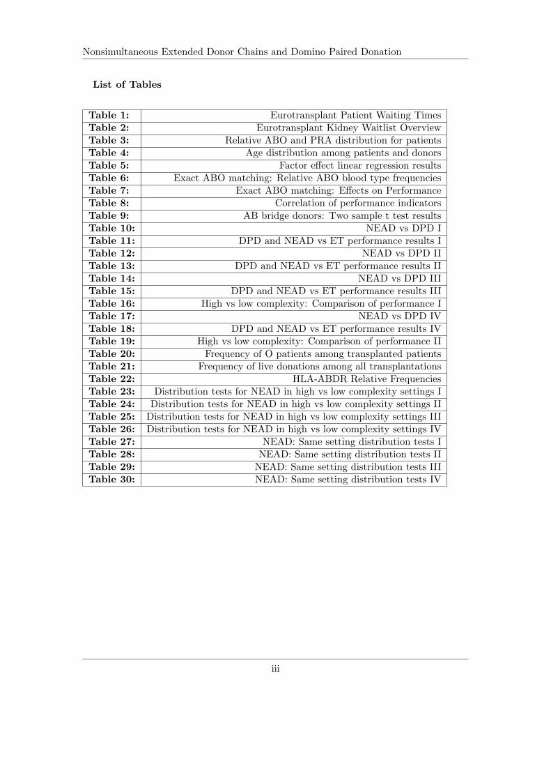
List of Tables
Table 1: Eurotransplant Patient Waiting TimesTable 2: Eurotransplant Kidney Waitlist OverviewTable 3: Relative ABO and PRA distribution for patientsTable 4: Age distribution among patients and donorsTable 5: Factor effect linear regression resultsTable 6: Exact ABO matching: Relative ABO blood type frequenciesTable 7: Exact ABO matching: Effects on PerformanceTable 8: Correlation of performance indicatorsTable 9: AB bridge donors: Two sample t test resultsTable 10: NEAD vs DPD ITable 11: DPD and NEAD vs ET performance results ITable 12: NEAD vs DPD IITable 13: DPD and NEAD vs ET performance results IITable 14: NEAD vs DPD IIITable 15: DPD and NEAD vs ET performance results IIITable 16: High vs low complexity: Comparison of performance ITable 17: NEAD vs DPD IVTable 18: DPD and NEAD vs ET performance results IVTable 19: High vs low complexity: Comparison of performance IITable 20: Frequency of O patients among transplanted patientsTable 21: Frequency of live donations among all transplantationsTable 22: HLA-ABDR Relative FrequenciesTable 23: Distribution tests for NEAD in high vs low complexity settings ITable 24: Distribution tests for NEAD in high vs low complexity settings IITable 25: Distribution tests for NEAD in high vs low complexity settings IIITable 26: Distribution tests for NEAD in high vs low complexity settings IVTable 27: NEAD: Same setting distribution tests ITable 28: NEAD: Same setting distribution tests IITable 29: NEAD: Same setting distribution tests IIITable 30: NEAD: Same setting distribution tests IV
iii

Nonsimultaneous Extended Donor Chains and Domino Paired Donation
List of Figures
Figure 1: Domino Paired DonationFigure 2: Non-simultaneous Extended Altruistic Donor ChainFigure 3: The Eurotransplant Kidney Waiting ListFigure 4: Graft Survival RatesFigure 5: Queue Development IFigure 6: Queue Development IIFigure 7: Queue Development IIIFigure 8: Adverse Effects of Bridge Donor Reneging IFigure 9: Queue Development IVFigure 10: Queue Development VFigure 11: Queue Development VIFigure 12: Adverse Effects of Bridge Donor Reneging IIFigure 13: Queue Development VIIFigure 14: Queue Development VIIIFigure 15: Adverse Effects of Bridge Donor Reneging IIIFigure 16: Queue Development IXFigure 17: Queue Development XFigure 18: Adverse Effects of Bridge Donor Reneging IVFigure 19: Adverse Effects of Bridge Donor Reneging VFigure 20: Distribution of Blood Type O Among Transplanted Patients
iv

Nonsimultaneous Extended Donor Chains and Domino Paired Donation
1. Introduction
As of 2011, many economists are concerned with kidney transplantations. However, itis not to the author’s knowledge that any of the economists who wrote on the topicin the past decade suffered or suffer from renal disease, required a live saving kidneytransplant, or do so now. The interest is rather, and indeed, an economic interest.
The reason for that is a new field of economics that seeks to integrate theory andpractice in designing markets. Economists have always had a theoretic interest in mar-kets but somewhat frowned on the managerial sciences that concerned themselves withthe not-so-scientific making and maintaining of markets and businesses. Fueled by theexpanding field of game theory, however, economists became more and more involved inthe creation process behind such important multi-billion dollar markets such as the onefor radio frequencies.1
Inspired by the newly gained knowledge about practical problems of markets, economistsbegan to explore other aspects than the equilibrium price. Only a few markets are ac-tually large and efficient enough to qualify for an analysis with the classical economictools. Most markets are governed by their own sets of rules and constraints. One veryimportant constraint, as Roth (2007) [44] stresses, is repugnancy.
A repugnant market, i.e. a market that a majority (excluding the participants) deemsdisgusting or distasteful, is often heavily regulated. There are historic and current exam-ples of markets with a questionable reputation, such as the markets for political favors(corruption), affection (prostitution), or cheap labor (slavery). Nevertheless, there isdemand and supply in these markets, no matter how much societies and states try toregulate or prevent them. While the regulation of the previously named markets mightbe unanimously advocated from an ethical standpoint, the prohibition of certain otherrepugnant markets generates massive negative externalities for the participants, such asdeath.
One such repugnant market is the market for organ transplants. Patients that need anew organ mostly face the problem that there is only one solution for a prolongation oftheir own lives, namely that somebody else dies and leaves an organ for them. End-stagerenal disease is such an illness that requires transplantation. For a while, patients canbridge the time until a transplant arrives with dialysis. The mechanical cleansing of theblood, however, can only last for so long. Veins get thicker and retract into the bodythe more often they are used to be attached to the dialysis machines. Patients can, infact, run out of access points for dialysis.
The kidney market has compared to all other markets for internal organs anotherfeature. Namely, that it is not necessary to die to donate. Each healthy human being
1Cf. Milgrom (2004) [30]
1

Nonsimultaneous Extended Donor Chains and Domino Paired Donation
can easily survive on one kidney and could donate one of the two he or she possesses.However, eliciting extra donations by paying for them is regarded repugnant in Westerncivilization.2 Hence, many patients suffer and die from the repugnancy-inspired rulesand regulations imposed on this market.
Economists have argued in two directions. The classic idea, the introduction of moneyto the market, was recently brought forward again by Becker and Elias (2007) [6]. How-ever, a new proposal has been developed. The field of market design, which will bebriefly introduced later, currently explores options to raise the efficiency of organ al-location while accepting the repugnant character of monetary exchanges. One way isthe promotion of Kidney Paired Donation (KPD) in which two pairs of incompatiblepatient-donor dyads donate crosswise. Economists calculated the most efficient way toconduct such exchanges and helped founding the New England Program for Kidney Ex-change (NEPKE).
Another opportunity are Nonsimultaneous Extended Altruistic Donor (NEAD) chains.These chains rely on ”good samaritans”: individuals who decide to donate a kidneywithout an intended recipient. A so gained transplant is offered to an incompatiblepatient-donor pair. Their now unused kidney is then offered to the next pair and so on.A second and conflicting view proposes the Domino Paired Donation (DPD) mechanismwhich advocates that the last donor in such a chain should not wait for the next pair toarrive but give to the kidney queue instead to keep donations simultaneous. These twomechanisms will be of central interest in this work.
The economic idea behind this thesis is to show how NEAD and DPD chains can in-crease allocation efficiency of altruistic donations while accepting the externally imposedrules of the market. Queue theory will be used to analyze the dynamic and evolving as-pects of the transplant waiting list for the case of Germany. The model will be extendedby diverse options to show how closer approximations of reality minimize or increaseeffects. Both mechanisms will be compared in four different settings to explore whichinstrument is better suited to ease the pressure on the market for transplants.
2One current example for a state that allows the purchasing and selling of organs is Iran. Cf. Ghodsand Savaj (2006) [20].
2

Nonsimultaneous Extended Donor Chains and Domino Paired Donation
2. Hypothesis
The question that is analyzed in this work is whether NEAD or DPD offers the moreefficient approach in allocating altruistic donors. This question has recently been dis-cussed vividly. NEAD proponents having the last word so far with an article by Ashlagiet al. (2011) [3] published in Transplantation. While both sides of the current debate arebacked by sophisticated simulations and their results, the discussion has solely focussedon the United States so far. In Germany, no large scale approaches have been attemptedto recreate the success economists have had by redesigning some of the tools in the mar-ket for kidney transplantations. Moreover, there have been no analyses regarding thepotential of the chain allocation mechanisms on full scale, not yet developed marketssuch as the German one. However, the purpose of this work is not to promote chainmechanisms for Germany but to show how the proposed policies work in markets theywere not intended for and assess the quality of their performance.
This work will differ in its setup from the work mainly done by Roth, Sonmez, andUnver (2005a, 2005b, 2007) [52, 50, 51] in allowing different preferences over compatibleorgans. Roth et al. had adopted the notion that patients were indifferent between com-patible organs, which is in accordance with the American literature on renal transplants.The European view differs and argues that patients distinguish between compatible or-gans by different classifications of quality. Therefore a simulation concerned with a Eu-ropean allocation system needs to incorporate this non-binary preference system. Thisleads to the first assumption, namely that Roth et al.’s results do carry over, regardlessof the preference structure.
The simulation itself is divided into two complexity settings. The different complexitysettings are modeled to give an impression of the basic effects both allocation policieshave in the low complexity setup and to analyze effects on the actual current waitlistsituation in Germany, simulated by a high complexity approach. Additionally, two dif-ferent time based perspectives are used for further analysis. First, a short term viewis employed to analyze the immediate effects of the introduction of chain mechanismsin comparison with the regular waiting list. In a second setup, long term effects afterimplementation will be of interest.
The argument in the literature between Ashlagi et al. (2011) [3] and Gentry et al.(2009) [19] has been whether DPD or NEAD mechanisms have an edge in increasingallocation efficiency. The DPD allocation argues a rather pessimistic viewpoint, namelythat bridge donors are likely to withdraw their consent. Hence, it would be wise to makeuse of their organs while they are still willing to donate. This gains an additional andsafe donation at the cost of letting the chain end. NEAD on the other hand argues veryoptimistically that each chain is potentially infinite and should be used to benefit thewaitlist. Regarding the vast numbers of transplants that could result from a continu-ous chain, NEAD accepts the risk of reneging. Both ideas have the theoretical abilityto increase allocation efficiency on the kidney market. The present work will analyze
3

Nonsimultaneous Extended Donor Chains and Domino Paired Donation
whether NEAD is actually the more effective mechanism in doing that.
Another aspect the simulation is designed to analyze is the sensitivity of NEAD andDPD mechanisms to changes in the setting. This is done in order to show how robustthese policies’ performance is in large scale applications. In the recent discussion, NEADis said to suffer heavily from increasing the Bridge Donor Reneging (BDR) rate, whichmeasures how many Bridge Donors (BDs) choose to revoke their consent to donate akidney and thus bring a chain to an end. A detailed explanation will follow in latersections. However, a central aspect of this paper is to show that NEAD is not per sesensitive towards BDR, leading to the overall hypothesis:
Hypothesis
Non-simultaneous extended altruistic donor chains hold an advantage overdomino paired donation policies in an integrated simulation of the Germankidney waiting list when compared regarding average queue length, waitingtime, and number of transplants, and maintain that advantage when addi-tional restrictions are imposed to which non-simultaneous extended altruisticdonor chains react less sensitive than comparable domino paired donationpolicies.
This hypothesis demands different capabilities of a fitting simulation. First, the cur-rent waiting list has to be constructed with valid data and both NEAD and DPD mech-anisms have to be modeled. Then, two setups - one for immediate and one for long termeffects - must be implemented. Finally, several options must be employed to enable astepwise approximation of the complexities encountered in reality.
Before results can be reported and interpreted, foundations have to be laid and thepaper proceeds as follows: Next, an overview of the development of market design eco-nomics and the literature on kidney exchange will be given. Following is backgroundinformation on the medical and legal situation, as well as the Eurotransplant organiza-tion and waiting list. Then, the basic theories the simulation was build on will be brieflyexplained. The subsequent section will be concerned with the data that was used toconstruct the simulation. Finally, the last three sections will cover a description of thesimulation itself, the reporting of the results, and the conclusion to summarize the mainpoints of this work.
4

Nonsimultaneous Extended Donor Chains and Domino Paired Donation
3. Literature Review
3.1. A brief history of Market Design
In hindsight, Market Design probably began when Gale and Shapley [16] published apaper in 1962 on allocation problems. The model they use describes the college admis-sions market and the marriage market which is more commonly used in Market Design.In the marriage market situation, there are men and women who wish to marry a suit-able mate of the opposite sex and whose preferences are complete and transitive. Galeand Shapley’s deferred acceptance algorithm provides a solution that is both stable andmakes truth-telling the dominant strategy for one side of the market.
Stability refers to the situation when there is no blocking pair to a market outcome,i.e. at least one man and woman who are not matched to each other but would like tobe. Stability is a powerful property and necessary for markets. Unstable markets havebeen empirically observed to unravel quickly.3 The dominance property comes very in-tuitively once the algorithm is understood.
The deferred acceptance algorithm makes one side of the market the proposing sideand the other the accepting side. In the first round, the proponents - let us say themen - walk up to their most desired woman and ask for her hand in marriage. Now,each woman has a list of proponents ranging from 0 to n, where n is the number of menavailable. Each woman ranks the men on her list according to her preferences for men.The most preferred men is kept and all others’ proposals are rejected. In all subsequentrounds, the men who are not matched propose to the next highest woman on their pref-erence lists. The women in turn reject all but the most desired of the proposing menuntil all proposals have been made. Since the men were the proposing side they havereached their best possible, stable match. Quick, intuitive proof:4 If not, there were aman (let us call him Dave) and a woman (Sarah) who assumingly like each other bet-ter than their current matches. That would, however, imply that Dave had previouslyproposed to Sarah, since she was higher on his preference sheet than his current match.In that case, Sarah had either rejected him because of someone else (maybe Larry) whoshe liked better or because he was not acceptable at all, the latter presenting a contra-diction to the assumption right away. In the former case, she is either still matched toLarry in whose favor she rejected Dave from the assumption or to someone else. Thefirst situation would again complete the proof right away. Another man being her hus-band currently would indicate that she prefers this man to Larry but since Larry wasmore preferred than Dave, she also prefers her husband to Dave by transitivity. A niceproperty of this result is that truth-telling is the dominant strategy when a deferred
3Cf. Roth (1991) [42]4The theoretic background, as well as technical proofs and the exact mathematical properties of thesets and spaces used will not be explained here. An understanding of the basics of market design isuseful to understand the purpose and workings of this paper but not essential. Cf. Gale and Shapley(1974) [16] or Roth and Sotomayor (1990) [47]
5

Nonsimultaneous Extended Donor Chains and Domino Paired Donation
acceptance algorithm is used.5
Roth and Sotomayor (1990) [47] developed the idea further from a one-to-one matchingin the marriage market to many-to-one matchings as in the market for college admis-sions. Students may apply to several colleges but only attend one while colleges canadmit more than one student. Roth and Sotomayor show that the results from the mar-riage market hold for the more general case with some exceptions and adjustments. Moreresearch followed and additional markets were explored with market design techniques.Policy makers got aware of that and started talking to economists. That led to theinvolvement of economists in restructuring malfunctioning markets. For example, Rothhelped redesign the United States National Resident Matching Program (NRMP) andthe school admission markets in New York and Boston.6 The NRMP fills over 20,000position for new physicians at hospitals across the U.S. each year. The problem of thatparticular market had been that with the increasing number of women in med schoolsthe number of couples who entered the match rose. Couples regularly try to get jobsclose to each other and the inability of the old algorithm to deal with that led to peopletrying to change the result of the match. Roth and Peranson (1999) [46] proposed andimplemented a new algorithm that stabilized the market. One lesson economists learnedfrom their involvement in actual markets was that a market’s efficiency is based on threekey elements.
Thickness, low congestion, and safety are necessary to keep a market stable.7 Thick-ness refers to the number of buyers and sellers that are in a market at the time tradesare allowed. If there are fluctuations in the numbers of available agents, markets tend tounravel. In the market for law clerks, for example, judges ask law students to work forthem as interns.8 Even though there were agreements on schedules for the procedure,offers were made at an exploding rate earlier each year. Students who were not able torespond quickly enough saw offers being taken back from the table within minutes. Acoordinative problem between the two sides of the market is usually the cause for thisprocess of unraveling that has been witnessed in many markets. This problem is mostlysolved by introducing clearinghouses.
A clearinghouse receives preference lists from both sides of the market and makesmatches at specific dates only. If the clearinghouse can be given the authority over amarket, the thickness of the market can be controlled easily by setting more or lessmatching dates. Hence, unraveling is halted and the market is back on track. Thesame applies if a market is too thick, i.e. congested. A clearinghouse brings a form
5There are some limitations, though, and results do not carry easily over to a many-to-one or many-to-many matching. Cf. Roth and Sotomayor (1990) [47], Ch. 5
6For the NRMP see Roth and Peranson (1999) [46] and for the admissions markets: Abdulkadiroglu etal. (2005a, 2005b) [1, 2]
7Summarized in Roth (2008) [45] and recently updated: http://kuznets.fas.harvard.edu/ aroth/papers/What have we learned update.Sept.2010.pdf
8Cf. Avery et al. (2007) [5]
6

Nonsimultaneous Extended Donor Chains and Domino Paired Donation
of structure that both market sides can easily use to orient themselves. And finally,safety is given since both sides are bound to the clearinghouse and ensuing matches arefinal. Mostly, participants who do not trust the other side to stick to its promises will at-tempt to negotiate back up plans. If trust into the clearinghouse can be established and asuitable allocation algorithm is used, truthfulness is the best strategy for all participants.
All the above effects obviously depend on the design of the clearinghouse which isone of the central tasks of market designers. Market design intersects with mechanismdesign, experimental economics, and game theory as Roth states.9 Essentially, thesethree disciplines enable the market designer to understand and implement mechanismsthat make a clearinghouse for a specific market safe, i.e. make algorithms strategy proof.Where truthfulness is the dominant strategy for all players, trust is established in themechanism of the market. Moreover, the economic engineer has to bear in mind thatpeople react to incentives. So, it might also be important to design rules for the marketto get participants to accept and use the clearinghouse. In many examples, the marketdesigner’s first and hardest task is to convince policy makers to surrender some of theirpower to the respective clearinghouse.10 In the early beginnings of the market for resi-dents, for example, hospitals made offers to students in only their second year of study.Such preposterous behavior was motivated by the fear to lose the top prospects to otherhospitals. However, nobody could foresee by their second year which students wouldbecome their class’s top graduates. Hospitals contracted students they did not want inthe end and students were forced to make decisions years before they became relevant.Medical institutions did not feel bound to the agreements not to recruit before certaindates because they did not trust their competition. This posed a multi-agent prisoner’sdilemma in which all hospitals were afraid the others could make their move first. Onlythe introduction of a clearinghouse and the stepwise agreement of all hospitals to onlymake contracts with students matched by the clearinghouse solved the market’s failure.Concluding, thickness, congestion, safety, incentives, and rules are the keystones to in-stall a working market.
Market design has evolved in several directions since the redesign of the NRMP algo-rithm by Roth and Peranson in 1999. On the theoretic frontier, Hatfield and Milgrom(2005) [25] have promoted important new theoretic insights with their paper on matchingwith contracts. While market design had seen one-to-one, many-to-one, and many-to-many matchings, matching with contracts considerably expanded the understanding ofexchanges. In their mathematical representation of an exchange situation, contracts aresolutions to complex systems of equations. A more thorough and complex modeling ofmarkets was made possible. Currently, papers are being developed and discussed thatallow for trades with middlemen, side payments, and other aspects that increase the the-oretic foundations of market design as a discipline.11 This will allow market designers to
9Cf. Roth (2002) [43]10Good examples can be found in the literature of the redesign of the Boston and New York school
systems. Cf. Abdulkadiroglu et al. (2005a, 2005b) [1, 2]11E.g. Hatfield and Kominers (2011) [24]
7
Nonsimultaneous Extended Donor Chains and Domino Paired Donation
understand and shape the driving forces of markets. Regarding the engineering aspectsof market design, economists have engaged in reshaping some markets. They face manyobstacles not foreseen by the economic standard literature. One such market is the topicof this work. The market for kidney transplants, specifically that for kidney exchanges.
3.2. Kidney Exchanges
The idea of kidney exchanges is that two or more of otherwise incompatible patient-donor pairs donate crosswise. Kidney exchanges are not particularly new as a topic forscientific papers. Rapaport (1986) [38] was the first to propose a registry for coupleswith incompatible donors. Ross et al. (1997) [40] also wrote on the subject of an in-compatible donor registry. Both papers have the idea in common that organized largescale exchanges could ease the pressure on the waiting lists. It has been the practicebefore and in some cases still is to simply assess that a donor is not suited for an EndStage Renal Disease (ESRD) patient for various reasons. It is the idea of the registriesto remember such couples and try to match them to other couples who are also mutuallyincompatible but match crosswise. Zenios (1998) provided the first statistical approachby proposing a queue theory model of the kidney waiting list which, however, does notapply to the present work as will be discussed later. The first economic work on kidneyexchange was done in the eponymous paper by Roth, Sonmez, and Unver in 2004 [49].
In their paper, Roth et al. acknowledge the situation for ESRD patients and proposethe Top Trading Cycles and Chains (TTCC) mechanism to allow multiple kidney ex-changes among otherwise incompatible donor-patient couples. Donor-recipient pairs aredenoted by (ki, ti) tuples where ki is the donor of pair i and ti the respective patient.There are also patients without donors and donors without patients (cadaveric kidneysor altruistic donors). Each patient has a set of compatible kidneys which is a subset ofthe set of all kidneys Ki ⊂ K =
�k1, k2, ..., km
�, where m refers to the number of kidneys
in the market. For the TTCC algorithm, each patient ti has a preference relation Pi
over Ki ∪�ki, w
�∀i ∈ (1, ..., n) which is his or her set of feasible kidneys, his or her own
donor’s kidney and the waitlist option w, where n is the number of patients. Because ofdifferent qualities and compatibilities of the kidneys it might be that a patient prefersthe waitlist to a certain renal transplant. Also, in this model patients can decide to giveup their donor’s kidney for someone else in order to jump to the top of the waiting list.A kidney may then be assigned to at most one patient while the waitlist option w canbe assigned to infinitely many.
The algorithm then works similar to the graph theory model of Shapley and Scarf(1974) [55]. In their paper, Shapley and Scarf report on the housing market where eachagent is assumed to be endowed with a house. For a trade, each agent points to thehouse he likes best and each house points to its owner. An agent may also point tohis own house indicating that he does not wish to trade. In each round, all cycles areremoved where a cycle refers to a situation in which all participants point to a house in
8

Nonsimultaneous Extended Donor Chains and Domino Paired Donation
the cycle and each house is pointed at by only one agent in the cycle. The simplest cycleconsists of one house owner pointing at his own house. In the simplest cycle in which atrade takes place, agent A points to house B, house B to agent B and agent B points toagent A’s house which points to agent A and completes the cycle. In Roth et al.’s 2004[49] paper the TTCC mechanism additionally allows for incomplete cycles - or w-chains- where the first patient receives a kidney from the waitlist and the last donor gives hisorgan to the waitlist. While cycles do not intersect, chains do. This implies that analgorithm has to chose between possible w-chains. Roth et al. name several possibilitiesespecially the prioritization of blood type O patients whose number of possible donorsis smallest among all patients.
The TTCC algorithm itself proceeds in four steps. First, all kidneys point to theirpaired patient and all patients point to their most preferred kidney or the waitlist option.Then each cycle is removed until there are no more cycles. If patients remain, the high-est chain chosen by a chain selection rule is removed. If patients remain, the procedurestarts from the beginning until no more patients are left unpaired. The authors showthat the so constructed algorithm with a simple chain selection rule is both efficient andstrategy-proof. Roth et al. continue to evaluate the potential gains through their TTCCmechanism by simulation. They conclude from the results that significant gains couldbe realized. Their work, however, had ignored on the one hand the heated debate on theethical feasibility of giving up a kidney for a high waitlist rank and on the other handthe logistical problems in realizing chains of size three and longer. Their follow-up workdeals with some of the arising problems.
In ”Pairwise Kidney Exchange” (2005a) [50], the same authors presented a modelsuited just for pairwise exchanges. Since multipair exchanges are difficult to handle fortransplant centers and hospitals (each transplantation procedure requires two operatingrooms and two surgical teams, a pairwise exchange then already requires four of each),the practicability had to be taken into account. Moreover, Roth et al. adjusted theirframework so that all patients are said to be indifferent between kidneys of the sameblood type - as long as they are not positively cross matched. This differs heavily fromthe notion used for the simulation in the present paper. Opelz (1997, 1998) [36, 35]and other authors have consistently advocated the European view that antigene com-patibility was an important factor in determining the quality of a transplant. Roth etal. instead follow the research of Delmonico (2004) [10], Gjertson and Cecka (2000)[21] and others who have argued to the contrary. The model Roth et al. develop isthen suited to the situation of 0-1, or binary preferences which is in turn not applica-ble to the European model. They develop a stochastic model based on graph theoryand the Gallai - Edmonds Decomposition lemma [17, 18, 11]. Their result of a strat-egy proof and efficient mechanism does, likewise, not carry over to the European market.
In a follow up paper from 2007, Roth et al. abstract from their kidney market modelto a more general approach. However, they again use the notion of indifference be-tween acceptable matches. As a result of their work on kidney exchanges, the authors
9

Nonsimultaneous Extended Donor Chains and Domino Paired Donation
helped founding NEPKE in collaboration with two physicians. NEPKE is essentiallya database, similar to the one proposed by Rapaport (1986) [38], in which informationabout incompatible patient-donor pairs is stored and used to find matches.12 In Europe,a similar attempt has been started in the Netherlands.13
3.3. Non-Simultaneous Altruistic Donor Chains and Domino PairedDonation
In 2006, Montgomery et al. [31] reported on a new procedure involving a so called NonDirected Donor (NDD). An altruistically motivated individual had shown up at JohnsHopkins Medical Center and offered his kidney for transplantation. Noting that thefrequency of such altruistic acts recently increased in the United States, Montgomeryet. al tried to maximize the effect of the donation. Instead of assigning the organ tothe first patient on the waiting list, the surgeons decided to offer it to an incompatiblepatient-donor pair from their kidney exchange program. The wife of a 48 year old pa-tient donated her kidney in turn to a patient from the kidney queue. The authors calledthis procedure a Domino Paired Donation (DPD).
Figure 1: Domino Paired Donation
Notes: Domino Paired Donation Chain with three pairs. AD: Associated Donor.
12Cf. Roth et al. (2005b) [51]13Cf. de Klerk (2005) [27]
10

Nonsimultaneous Extended Donor Chains and Domino Paired Donation
Also in 2006, Roth et al. [48] reported on a similar occurrence and proposed a mecha-nism which Rees et al. [39] coined a Nonsimultaneous Extended Altruistic Donor(NEAD) chain in a 2009 paper. Building on previous papers, Roth et al. developed analgorithm that uses either patients who are willing to exchange their associated donor’skidney for a high waitlist rank or NDDs. In either case, a kidney becomes available thathas no intended recipient. In contrast to the proposal brought forward by Montgomeryet al., Roth and colleagues argue that the last donor in such a chain should wait for anew possibility instead of donating to the wait list. In that case, when couples A, B, andC have participated in a chain started by a NDD, couple C’s donor would wait for thenext compatible couple instead of donating to the queue. So, the algorithm which thispresent work also uses, consists of finding all possible chains and choosing one of themaccording to an arbitrary rule, e.g. length. This is only simple in theory, since multiplesets and subsets of patients and donors have to be compared regarding said arbitrarycriterium. The description of the mechanism used in this thesis follows in Section 7.Note that there is no explicit theoretic framework anymore, since this is detached fromthe TTCC algorithm which was based on non-binary preferences.
Figure 2: Non-simultaneous Extended Altruistic Donor Chain
Notes: Non-simultaneous Extended Altruistic Donor Chain with three pairs. AD: Associated Donor.
Before chains were introduced, the problem had been KPD’s requirement of simultane-ity. Pairs only agree to exchange kidneys when it is safe that neither donor suddenlywithdraws his or her consent while the other donor has already undergone surgery. In
11

Nonsimultaneous Extended Donor Chains and Domino Paired Donation
that situation one pair would lose its bargaining chip and suffer a great loss, indeed.This requirement of simultaneity could be removed in non-simultaneous exchanges, i.e.NEAD chains. If in such a setting a donor rethinks his or her decisions, the other pairstill has a donor kidney. So, in the worst case the chain would come to an end but nopair would lose a kidney.
The difference between the two approaches is mainly based in the question whetheror not to allow for non-simultaneous exchanges in which donors have the possibility torevoke their consent. In subsequent papers, Montgomery’s colleagues in Gentry et al.(2009) [19] and Ashlagi et al. (2011) [3] have promoted their respective views. Gen-try’s paper argues that there is no significant difference between the approaches whenconstraining the chain length to three simultaneous transplantations. Under this as-sumption, Gentry et al. show that there is, in fact, a small imbalance in favor of theDPD approach compared to the NEAD mechanism. In Ashlagi et al.’s 2011 reply, thecounterargument relies on the chain length. In their opinion, chain length is not decisivebut elapsed time between segments. Their rationale is that a segment will continue ifthe time is sufficiently short and hence, should be counted as just one segment. Forexample, two consecutive chain segments that take place within days should count asone chain at a length of six. Therefore, chain segments could be well longer than three.This argument is built on the notion that it is not that common for the last donors ofchain segments - so called bridge donors (BDs) - to renege. Gentry et al. assume that adonor who is kept waiting will eventually reevaluate his or her situation and change hisor her mind. Ashlagi et al. counter that this will only take place when a lot of time haspassed.
In their response to Gentry et al. (2009), Ashlagi et al. (2011) make use of a dy-namic simulation over 8 and 24 periods for a rather small scale model. They use datafrom the Alliance for Paired Donation (APD) to come as close as possible to the actualsituation this organization faces.14 In their approach, Ashlagi et al. allow for differentchain lengths, bridge donor reneging, patients rejecting an organ for different reasons,and diverse other medical criteria. Almost all of these considerations can be found inthe setup of the present paper’s simulation as well. However, intra-chain bridge donorreneging which the authors discuss is neglected in the present work. Intra-chain renegingrefers to a situation when a bridge donor has to wait for a relatively short time interval(a day) to continue an already matched chain. Since it can justly be argued that suchshort time will seldom have an important influence on a grave decision such as the oneto give a kidney, short term reneging is assumed to be zero for simplicity. The moreinteresting feature is inter-chain reneging which occurs after a chain is completed. Then,the bridge donor has not been assigned a match and has to wait to begin a new chain.The higher the probability for him to rethink his or her decision and renege, the greater
14For the present paper, it has to be noted that a clearinghouse has been established neither for Europeas a whole nor for Germany and data for NDDs is largely speculative. This approach is used toanalyze potential effects on the whole market rather than on a small subset.
12

Nonsimultaneous Extended Donor Chains and Domino Paired Donation
the benefit of the DPD mechanism, where the final bridge donor donates to the waitinglist right away. This will be of interest to the analysis presented in this work and willbe explained in detail later. The key argument by Ashlagi et al. is that imposing con-straints on the chain length - as Gentry et al. did - has the most limiting effect on NEADmechanisms compared to DPD. Therefore, Ashlagi et al. argue that NEAD is more sen-sitive to Chain Size Limits (CSLs) than DPD. This will be analyzed in detail in this work.
Another important point of discussion is the assumed blood type distribution of livedonors. Both Gentry et al. and Ashlagi et al. are concerned with exchange programswhich have a large portion of blood type O patients. This is mostly due to the fact thatblood type O is hardest to match since those patients are incompatible to all other bloodtypes. Therefore, the distribution of live donors is of interest since the impact on theblood type O heavy waitlists is larger the more O donors are available. For the presentanalysis, however, that is of little interest since there are no exchange programs eitherfor the whole of Europe or for Germany. Hence, there are also no pools of incompatiblepatient-donor pairs. The distribution of blood types in transplanted patients will beanalyzed, nevertheless, but not be of central interest.
In this work, the two positions are contrasted with a dynamic approach. The simu-lation featured in this paper is built on a queueing theory platform to make changes inthe waiting list setup visible. Before the simulation and results can be reported, somemore groundwork has to be laid which will take place in the ensuing sections.
13

Nonsimultaneous Extended Donor Chains and Domino Paired Donation
4. Background
4.1. Medical Background15
Human beings differ from each other not only on a personal level. Some develop lifethreatening diseases that require transplantation and others do not. On the geneticlevel, our bodies have each a unique setup. When looking for a genetic match in order totransplant an organ, three major obstacles need to be overcome. First, the ABO bloodtype has to match. Then the six humane leucocyte antigenes for A, B, and DR allelesare compared and finally, a cross match must be negative. The following section willintroduce these three steps of the matching process and explain them as far as necessaryfor the purposes of this work.
The human body is equipped with two kidneys which are responsible for cleaning theblood - until they fail. High blood sugar, high blood pressure, and diabetes are the maincauses for ESRD, which is by far the top reason for patients to join the kidney waitinglist.16 Only after several attempts to safe a patient’s own organs and only after the kid-neys’ filtration rate has dropped under a certain threshold, a patient is declared to haveentered the end-stage of renal disease. At that point, the consulting physician conferswith his or her patient and potentially submits a patients data to the organ waitingqueue. Since it is very unlikely to find a match right away for most patients, the timehas to be bridged by dialysis. Dialysis refers to the cleansing of the blood with the helpof machines or dialysate. All dialysis methods, however, can lead to complications andbear some risks for the patients. In most cases, a transplantation will become inevitableand therefore, patients often enter the waiting list as soon as possible. The ensuing wait-ing time depends on several characteristics of the patient’s body: blood type, HumaneLeucocyte Antigene (HLA), and the immune system.
Each and every human being has one of the four blood types O, A, B, and AB. Theseletters basically refer to the surface structure of the blood cells by which the body rec-ognizes them. Important from a designer’s perspective is the compatibility matrix. Opatients are labelled the general donating patient because they may donate to anyonesince their blood is compatible with all other blood types. AB patients are on the otherend and referred to as the general receivers, their bodies can cope with all other bloodtypes. Generally, blood type O is compatible with O, A with A and O, B with B andO, and AB with A, B, AB, and O. However, in addition to the general compatibility, apatient might be sensitized to a certain blood type. This happens, for example, when apatient is a mother whose blood was mixed in the birth process with that of the child.Her immune system subsequently reacted to the child’s blood. In that case, there arestill t-cells in her blood that remember the structure of the foreign proteins. As soonas a similar cell enters the sensitized patient’s system, her immune system reacts. An
15The author wishes to thank Drs M. Lindemann and F. Heinemann of the German Society for Im-munogenetics for the many helpful explanations.
16E.g. Klag et. al (1996) [26]
14

Nonsimultaneous Extended Donor Chains and Domino Paired Donation
organ with that blood type would be rejected by her body. Sensitization can also occurwhen a patient had prior transplants or blood infusions that were rejected.
Nevertheless, when blood types match, other factors have to be checked before anorgan is assigned to someone. The humane leucocyte antigene (HLA) is also importantin determining how well a kidney might fit a patient. For transplantation, HLA-A, -B,and -DR alleles are considered. These alleles are inherited one from each parent. Thatimplies that for siblings or first degree blood related patient-donor pairs, there is a 25%chance that all antigenes match, a 50% chance that at least some match and a 25%chance that none match. The maximal match is then six, when both maternal and pa-ternal HLA-A, -B, and -DR alleles are the same in both subjects, then five, four, three,two, one and finally, no match.
HLA alleles have been known to medicine since the 1960s. Since then science hasdiscovered dozens of new alleles and started to understand them better. B and DRantigenes belonged to the group of A antigenes before a significant difference was found.For matching purposes the broad antigenes of the A and B groups as well as the DRsplit antigenes are compared between donor and receiving patient. Broad antigenes referto more general alleles that in many cases break down to subgroups. For example, theHLA-B12 allele is a broad antigene that can decompose into B44 or B45 split antigeneswhich in turn could be more accurately identified as B4401, B4402, and so on. As said,only broad antigenes for A and B and split antigenes for DR alleles are considered inthe context of transplantation.
It is disputed between the U.S. and Europe whether HLA matching is important ornot. In the United States the importance of HLA matching has continuously diminished.Studies found that there was no significant difference between full and no matches withinthe first year17. It was also found that for subsequent graft survival rates only the HLA-DR factor had some level of significance. Hiowever, Eurotransplant is still making use ofthe HLA match, relying on other studies that have disputed the irrelevance of HLA forgraft survival.18 Adding to the American view is the evolution of immunosuppressivedrugs. Different chemicals have been developed that allow patients to live with organsthat would otherwise be attacked by their immune systems. The disadvantages of thatare clearly the thereby weakened immune system and related dangers such as heightenedcancer probabilities.19 The suppression of the immune system becomes more and moreprevalent, though, and leads to increasing graft survival rates. Especially the negativeeffects of poorly matched HLA alleles can be reduced. HLA matching remains, however,an important part of the medical assessment in Europe. As a technical note, this lead tothe rejection of binary preferences as a sound assumption for European patient behavior.
17Cf. Gjertson and Cecka (2000) [21] or Cecka (2001) [8]18E.g. Opelz (1997, 1998) [36, 35]19E.g. Guba et al. (2004) [23]
15

Nonsimultaneous Extended Donor Chains and Domino Paired Donation
Even after blood type and HLA are a perfect match, an organ could be rejected by therecipient body if the cross match is positive. The cross match is a procedure that mixesserum (a blood derivate) from the donor and the recipient. A cross match is positive ifthe recipient’s white blood cells react hostile towards the donor’s serum. In that case, atransplantation is not feasible. The probability that a recipient reacts to a foreign organis measured by Panel Reactive Antibodies (PRA) or panel reactive antibody. The higherthe PRA the higher the probability of a positive cross match. The PRA is obtained byapplying the patient’s serum to an industrially manufactured panel that contains mostHLA alleles. The idea is for the panel to mirror the frequency of each allele in the re-spective population. For the case of Europe, for example, the A2 allele is found in about50% of the population. A fitting PRA tester should then have 50% of its surface filledwith A2 alleles. A positive reaction towards A2 would then indicate a PRA of 50%. Notethat the PRA percentage is not proportional to the number of alleles a patients reactsagainst but to the prevalence of these alleles. Moreover, the problem in manufacturingsuch testers is to get the proportion of the alleles right. When asked about it, Dr. F.Heinemann said that most testers do not accurately mirror the prevalence of alleles andtherefore the PRA is never absolutely accurate.20
Finally, age and overall condition do also play in the medical assessment process. Apatient’s age is first of all, cynical as that may sound, an indication of the remaining timehe or she has left and whether a transplantation makes sense. Moreover, transplants arealso chosen considering how long the graft will survive. Transplanting the kidney of a 70year old into a 16 year old would be rather infeasible. In addition to the problem of graftsurvival rates, an old organ is more prone to fail. Therefore, a quick reentering to thewaiting list of the patient would be foreseeable. Furthermore, there are several illnessesand situations which demand multiple transplantations for a patient. Very common is,for example, the combination of kidney and pancreas. Mostly patients suffering fromtype 1 diabetes whose pancreas does not produce sufficient amounts of insulin need bothorgans. Other criteria can also influence the medical assessment. A malicious canceror a history of heavy substance abuse might play into the decision of whom to give atransplant. The aim for all medical personnel involved in the process is to balance riskand benefit for each patient.
Concluding, a medical assessment includes several comparisons and matches. ABOblood types must be compatible. Then, HLA-A, -B, and -DR alleles are compared andthe more of the six alleles match the higher the graft survival chances. Finally, a crossmatch is used to verify that a patient’s immune system does not react towards the spe-cific HLA combination of the respective donor. If all criteria match and the overallsituation of the patient allow for the transplant, it is medically feasible to perform theprocedure.
20Recently, Eurotransplant’s Tissue Typing Committee has switched from using the %-PRA values tothe v-PRA, which is a measure of frequency, as explained in the Eurotransplant Annual Report 2010[34], p. 28.
16

Nonsimultaneous Extended Donor Chains and Domino Paired Donation
4.2. Kidney Transplants Overview
On May 31st 2011, 7,730 Germans were in need of a new kidney. In the whole Eurotrans-plant21 area, covering also Austria, Belgium, Croatia, Luxembourg, the Netherlands, andSlovenia, a total of 10,412 patient were waiting for a live-saving kidney transplant. How-ever, only 1,474 kidney transplants had been performed through Eurotransplant (832 forGermany) from January 1st till May 31st.
Figure 3: The Eurotransplant Kidney Waiting List
1969
1971
1973
1975
1977
1979
1981
1983
1985
1987
1991
1993
1995
1997
1998
1999
2000
2001
2002
2003
2004
2005
2006
2007
2008
2009
2010
020
0040
0060
0080
0010
000
1200
0
020
0040
0060
0080
0010
000
1200
0
!
!
!
LegendActive Waiting ListCadaveric KidneysLive Donor Kidneys
Notes: Numbers as reported by Eurotransplant Annual Report 2010 [34]. Cadaveric Kidneys refer onlyto transplanted kidneys from deceased donors.
The development of the waiting list in comparison to the number of available donorsis illustrated by Figure 3. Despite the recent decline in numbers for the active waitinglist, the number of waiting patients still exceeds the number of available donors by over5,000 per year. The critical mismatch between donor and patient numbers is the centralproblem ESRD patients face. Of 10,533 patients who were still waiting for a kidney atthe end of 2009, 1,755 had been on the waitlist for more than five years. Taking thebeginning of dialysis as basis for the waiting time calculation the number increases to3,086 patients. According to de Fijter (2010) [14], the median waiting time for a kidneyfrom a deceased donor is more than four years for all Eurotransplant member countriescombined and significantly higher in Germany (for current data see Table 1).
21Eurotransplant is the international legal authority for maintaining the organ donor wait lists of itsmember countries.
17

Nonsimultaneous Extended Donor Chains and Domino Paired Donation
Table 1: Eurotransplant Patient Waiting Times
Waiting time in years based on beginning of dialysis based on time entering waiting list
0 - 1 17.3% (21.8%) 41.9% (46.6%)2 - 4 45.7% (46%) 38.3% (37%)> 4 35.2% (28.6%) 19.8% (16.4%)
Notes: Waiting times for 2010. European numbers in brackets. Source: EurotransplantAnnual Report 2010 [34].
In talking about donation one has to distinguish between live and cadaveric donation.Live donation has seen an increase by over 40% over the last years and by now 25% ofoverall transplanted kidneys allocated by Eurotransplant stem from live donors.22 Thisdevelopment benefits the patients. Figure 4 shows how live donation affects 1-5 yearsurvival rates of transplants, which are also called a grafts. Evidently, live donationleads to a lower probability of reentering the waitlist and hence, a higher quality of live.Both NEAD and DPD introduce additional live donors into the market by activatingthe pool of incompatible donors. Therefore, it will be interesting for the analysis to seehow both quantity and quality of transplants will be affected by chain allocation.
Figure 4: Graft Survival Rates
Years after Transplant
Gra
ft Su
rviva
l Rat
e
1 year 3 years 5 years
60%
70%
80%
90%
100%
!
!
LegendCadaveric KidneysLive Donor Kidneys
60%
70%
80%
90%
100%
Notes: Data taken from OPTN, based on numbers for the United States. 1 year survival based on2002-2004 transplants, 3 year survival based on 1999-2002 transplants, 5 year survival based on
1997-2000 transplants. Source: http://optn.transplant.hrsa.gov/latestData/rptStrat.asp. Accessed onJune 9th, 2011.
22Increase from 901 in 2006 to 1262 in 2010, numbers for the whole Eurotransplant area. EurotransplantAnnual Report 2010 [34], pp. 60 - 61.
18

Nonsimultaneous Extended Donor Chains and Domino Paired Donation
When simulating donors and interpreting their numbers, it is necessary to develop abasic understanding as to what motivates or prevents them from making a donation. Amain factor in a (live) donor’s decision to give a kidney is, of course, the mortality ratefor donors. Segev et. al (2010) [54] reported that for the U.S. the probability of dyingduring surgery was at 0.031%. Moreover, the authors found that 25 donors died within90 days of the transplantation. Furthermore, long term survival rates are reported tobe not affected by the procedure. Another fear for many donors is to require a trans-plant themselves later in life. Sommer et al. (2004) [56] observe that the probabilityfor previous donors to develop an ESRD is at 0.2 - 0.5%. Additionally, most organallocation organizations have adopted regulations that move transplantation-requiringprevious donors on top of the waiting list.23
Another important factor for patients on the waitlist is the time they will have towait. As said, the average patient has to expect to wait for many years. However, thereis another negative externality for patients besides fear whether a transplant will reachthem in time. When not equipped with a functioning kidney, the body goes into decay,irrespective of dialysis. Meier-Kreische et al. (2000) [29] reported that four years ofwaiting time decreased survival chances by 72% compared to an immediate transplant.This clearly stresses that waiting time is an important factor, which is why it will beused as a performance indicator in the later analysis.
These findings illustrate that the central economic interest in adjusting the market ofkidney allocation is efficiency. NEAD and DPD allocation have the theoretic ability toincrease both quality and quantity of transplants while accepting the repugnant charac-ter of monetary transactions. However, the rules of the market consist not only of theconsensus regarding money but also of their legal enforcement through laws. Currently,Eurotransplant reports 32 altruistic donations per year which means that 32 personsdecide to undergo surgery to give one of their functioning organs to someone they donot know and will not get to know in most cases.24 Their only aim is apparently to helpa fellow human being. None of the donors come from Germany because in Germany,altruism is a federal offense.
4.3. Legal Situation
As most Western countries, Germany has dedicated a special law to the transplant mar-ket. The Transplantationsgesetz rules that it is unlawful to trade or otherwise exchangean organ for valuable consideration. Moreover, it is illegal to anonymously and altru-istically donate a kidney. Such behavior is punishable by law with up to five years ofimprisonment25. The aim of the law is obviously not to rule out altruism. However,legislators included exchanges without payments in the list of unlawful actions and ef-
23Cf. Roth et. al (2005a) [50]24Cf. de Klerk et al. (2005) [27] for a discussion of anonymity in kidney exchanges.25Article 18 (1) Transplantationsgesetz
19

Nonsimultaneous Extended Donor Chains and Domino Paired Donation
fectively prevented altruistic donation. Another solution is offered by the United States,where the National Organ Transplant Act (NOTA) states that “it shall be unlawfulfor any person to knowingly acquire, receive or otherwise transfer any human organ forvaluable consideration for use in human transplantation”. However, anonymous andaltruistic donations are expressly excluded and the 2007 Charlie W. Norwood LivingOrgan Donation Act amended the National Organ Transplant Act by adding “The pre-ceding sentence does not apply with respect to human organ paired donation.”
Pairwise exchanges were also considered unlawful in Germany until the Bundessozial-gericht, the Federal Social Court, ruled in favor of a German couple that had beenaccused of organ trade. The couple had exchanged kidneys with a swiss couple inZurich. The court ruled in October 2003 that it was possible to form a sufficiently sta-ble relationship between two previously unacquainted couples for the purpose of kidneyexchange. However, the article was upheld which demanded such a relationship. Thatmeans that altruistic donation is still illegal if the recipient is unknown and not suffi-ciently acquainted to the donor.
Pairwise exchanges have taken place more often since the courts ruled but their num-bers are still neglectable. The medical centers of a few universities, such as Essen,Dusseldorf, or Cologne,26 run small scale programs and have conducted exchanges. Therehas been no attempt to organize these efforts, however. Likewise, there has been no at-tempt to start a NEAD chain. This negligence is caused by the strictness of the Germantransplantation law. There are in fact no altruistic donations and pairwise exchangedoes not take place on a large scale. This has also been attributed to the absence ofeconomic analyses of the situation.27
As for the feasibility of NEAD or DPD chains in Europe, the German characterizationof altruism as a crime has to be acknowledged. A direct approach is not advisable sinceeven the attempt to donate altruistically and anonymously is punishable28. However,since the courts ruled that a sufficiently thick relationship can evolve from previousmeetings that might be a method worth considering. Another way seems to be theadjustment of legislation which has been discussed for several years now. While thequestion of an opt-out procedure to get more citizens to become organ donors has beenprimarily focussed on29, the ban on anonymous donations could be lifted, too. However,both avenues of approach are speculative. Since, as stated, the purpose of this work isnot to promote political action but to show how market design tools work on differentmarkets a further speculative discussion is omitted. For the purposes of this work it willbe assumed that either German legislation has changed or another avenue of approachhas been chosen similar to the circumvention that made kidney paired donations feasible.
26Cf. Witzke et. al (2005) [58]27One recent attempt by Breyer and Kliemt (2007) who focus on cadaveric donation.28Article 18 (3) Transplantationsgesetz29Cf. Breyer and Kliemt (2007) [7]
20

Nonsimultaneous Extended Donor Chains and Domino Paired Donation
4.4. Eurotransplant
This work will focus on Germany and the German waitlist. However, Germany has giventhe authority to allocate organs to Eurotransplant (ET) which will therefore be brieflydiscussed. Eurotransplant is the international authority that also maintains the waitinglists of five other European countries besides Germany. The agency was founded in 1967by the dutch physician Jon van Rood and started with twelve participating transplantcenters. The idea of van Rood was to create a large enough pool to find good HLAmatches for each patient. Previously, regional transplant centers where responsible forfinding a match which relied solely on ABO blood type matching. Today, Eurotrans-plant handles the allocation of kidneys from and to Austria, Belgium, Croatia, Germany,Luxembourg, the Netherlands, and Slovenia. To facilitate the allocation of kidneys, theEurotransplant Kidney Allocation System (ETKAS) was implemented.
ETKAS was introduced in 1996 to deal with some difficulties in the allocation processand still defines the rules for the matching. Patients are ranked across several charac-teristics. Among them waiting time, location, age, HLA match, PRA level, and highurgency. This matching is while it is by far the largest30 not the only allocation pro-gram employed by Eurotransplant. In addition, smaller programs especially for seniorsand highly sensitized patients were introduced. The latter ranks patients who have ahistory of being highly immunized ahead of the regular queue. Seniors older than 64who participate in the Eurotransplant Senior Program (ESP) are assigned kidneys fromcadaveric donors aged 65 and older without HLA matching. Both the program for highlysensitized patients, the acceptable mismatch (AM) program, and the ESP program areneglected for the purposes of this research. Instead, the ETKAS score system is used torecreate a similar ranking in the implemented matching algorithm.
30It handles about 64% of the German allocation. Eurotransplant Annual Report 2010 [34], p. 55.
21

Nonsimultaneous Extended Donor Chains and Domino Paired Donation
5. Theory
The analysis in this paper is based on some basic theories and work done by othereconomists involved in the field of market design, most prominently Professor Alvin E.Roth31. As for the econometric foundations, mostly queueing theory is made use of tobuild a process of incoming renal disease patients waiting for a suitable organ. The sim-ulation itself was extended to allow for numerous options that have been discussed in theliterature. These options are intended to make the simulation more realistic with everyadditional extension and will be presented in the corresponding section. Nevertheless,a complete reproduction of reality can hardly be achieved and as in any econometricmodel, some generalizing assumptions have to be made that will also be discussed inlater sections.
What is omitted here is the general discussion of the basic framework in which chainmatching theory was developed. It was developed as an addition to the pairwise ex-change algorithm which relies heavily on graph theory. The theory itself is not foundedon a specific model which makes it less tangible but rather a collection of algorithmsand mechanisms. Moreover, as earlier explained, the results Ashlagi et al. (2011) [3]calculate are founded on the Gallai - Edmonds decomposition lemma [17, 18, 11] whichrequires binary preferences of market participants over the object in question. That isby assumption the case for northern America. European doctrine, however, ranks organsby several classifications, one of them HLA matches. Since quality is not a dimension forevaluation in Ashlagi et al.’s framework, they can apply elegant graph theory solutions.While the main assumption of this work is that this approach can be transferred with-out loss of generality to the non-binary European market, a theoretic solution cannot beoffered. Rather an experimental approach is chosen. The algorithm itself simply choosesone chain of all possible chains by some arbitrary rule. Since the idea of the algorithm isvery intuitive and graph theory cannot be used for an European, non-binary transplantmarket, an introduction to graph theory is omitted. In this section, the basic theoriesdriving the chosen computational approach are presented.
5.1. Stochastic Processes
Stochastic processes are ways of quantifying the dynamic relationships of se-quences of random events.
- Taylor and Karlin (1987) [57], p. ix
A stochastic process is, technically speaking, a family of stochastic variables on anindex set T. T can be both discrete or continuous, the latter being the case for thepresent paper. Since this definition is as short as it is abstract, an example might be in
31Cf. generally: Roth (2002) [43], Roth and Sotomayor (1990) [47], and specifically kidney exchange:Roth et al. (2004, 2005a, 2005b, 2007) [49, 50, 51, 52] or most recently, Ashlagi and Roth (2011) [4].
22

Nonsimultaneous Extended Donor Chains and Domino Paired Donation
order. Consider a week and you are interested in the hours of sunlight on each day, sinceyou would like to go to the beach on every day(it is your only vacation this year). Eachday is a random variable in that it is not clear before how many hours of sunlight willbe there for you to enjoy. So, the index set would be T = {monday, tuesday, wednesday,thursday, friday, saturday, sunday}. When X is the hours of sunlight on a given dayand that number is random, Xt, t ∈ T is a stochastic process.
Some additional properties need to be introduced quickly in order to explain the simu-lation later more thoroughly.32 Stochastic processes are said to be (weakly) stationary ifthe first and second moments of their underlying stochastic distributions do not changewith respect to t, i.e. E(X(t)) = µ and γ(t, s) = γ(t − s)∀s, t ∈ T . Applying this tothe sunlight example, Xt would be (weakly) stationary if the a priori expected value forhours of sunlight was the same for each day and the variance between four days was notdependent on whether it was monday to thursday or tuesday till friday but only on howmuch time has passed between the two days.
A process is said to have the Markov property iff
P (Xt ≤ xt|X1 = x1, X2 = x3, ..., Xt−1 = xt−1) = P (Xt ≤ xt|Xt−1 = xt−1),
which means that for the probabilistic assessment of Xt it is sufficient to know the real-ization of Xt−1. A stochastic process that exhibits that property is also called a Markovprocess. The sunlight example seems to be markovian. Meteorologists might beg to dif-fer but for this example the assumption might stand that it is not important for guessingsaturdays weather on friday whether it rained on tuesday or not. An example for whichthe Markov property does not hold is the performance of a football player. A long his-tory of bad performances is not swept away by one good game in his or her case. Arrivalrates for ESRD patients on the waiting list, however, can fairly be called markovian. Astochastic process with the Markov property that well describes this phenomenon is thePoisson process.
5.2. Poisson Processes
Poisson processes describe frequencies of occurrences of certain events, such as arrivalsof patients on a waiting list. The huge advantage of Poisson processes is that they areas simple as versatile and accurate. Choosing a Poisson process as the basis of a sim-ulation of a queue process comes quite naturally if one assumes that arrival rates areindependent from each other, i.e. patient A does not decide to join the waitlist earlier orlater because of patient’s B presence there. An additional necessary assumption is thatthe probability for an event to occur on a given interval is proportional to the length ofsaid interval. Both assumptions can fairly be made for the case of ESRD patients which
32Note that these introductions are far from being detailed and will not make use of any proofs forreasons of shortness and simplicity. For a more detailed introduction see Taylor and Karlin (1984)[57] or Norris (1997) [33].
23

Nonsimultaneous Extended Donor Chains and Domino Paired Donation
is why the Poisson process was chosen as a basis for the simulation and as the fittingstochastic process.
A stochastic variable (X) is said to be of a Poisson distribution (X ∼ Poi(λ)) iff
P (X = a) =λa
a!exp(−λ), a ∈ N,
E(X) = λ,
V ar(X) = λ.
A stochastic process with a non-negative, integer-only sample space, is referred to as aPoisson process iff
X(s) ≤ X(t), s ≤ t,
N(0) = 0,
P (X(t)−X(s) = i) =
�λ(t− s)
�i
i!exp
�− λ(t− s)
�.
Additionally, the underlying stochastic process is required to have independent incre-ments, which means that not overlapping intervals that are subsets of the index set arestatistically independent.33
Regarding it’s moments, a Poisson process is not stationary for any λ > 0 since
µ(t) = λt.
It’s auto-covariance function is defined as
γ(s, t) = λ min{s, t} (hence, µ(t) = V ar(X(t))).
The instationarity of the process comes quite intuitively when regarding the fact thatthe process is not decreasing and
P (X(t) ≥ 1)t→∞,λ>0
= 1.
Since the probability of two events happening at the same time is zero:
P (X(t)−X(s) ≥ 2)s=t=
�λ(t−t)
�ii! exp
�− λ(t− t)
�= 0
33For a more detailed introduction, see e.g. Taylor and Karlin (1984) [57]
24

Nonsimultaneous Extended Donor Chains and Domino Paired Donation
the process’s increments are always one. Therefore, the true interest is in the time whenan increment takes place. Luckily, a homogeneous Poisson process (which is the only oneused in this paper) has independently and identically distributed intervals following anexponential distribution with rate 1
λ which makes the simulation of the arrival processesvery comfortable. As a reminder, the exponential distribution’s density function was:
f(t) = λexp(−λt), t ≥ 0
and the distribution function:
F (t) = 1− exp(−λt), t ≥ 0
The fact that a homogeneous Poisson process necessarily requires intervals to be iidexponentially distributed implies that the first patient’s arrival time can be simulated asa random number from the exponential distribution with the patients’ arrival rate λp.The second patient’s arrival time is then the first patient’s time plus another randomnumber from the exponential distribution. Hence, the vector of arrival times can becalculated as the cumulative sum of n draws from the exponential distribution, where nis the number of patients. Reneging times can then be calculated by drawing n randomnumbers from the exponential distribution and adding them to the arrival times. Forthe incoming kidneys, only arrival times need to be simulated which can be done thesame way as for the patients with the kidney arrival rate λk instead.
As a final piece of theoretic background, it is necessary to understand how Poissonprocesses are used to created a dynamic system that leads to the formation of a queue.
5.3. Queue Theory
The phenomenon of the queue is a well known annoyance in everyday life. People whohappen to want a particular thing that can only be obtained at a certain location get inline and wait for their turn. It happens at the cinema, at the supermarket, and unfortu-nately also at the transplant clinic. Only in the latter case people do not literally get inline. While movie goers and shoppers might leave the queue after some time because ofanger for not being served, ESRD patient renege because they either become inoperableor die. A theory that enables researchers to analyze processes with such behavior isqueueing theory.
Queueing theory began as a stochastic model built by Erlang34 (1909) [12] to un-derstand the complexities of the then emerging automatic telephone exchange system.Today, queue theory is mostly used for queueing networks in complex systems such ascomputers. Its analytic power is necessary to understand how data is moved betweenprocessors and memory banks and how to design them to be more efficient.
34After whom also the distribution is named which one arrives at when calculating a queue by the abovementioned method.
25

Nonsimultaneous Extended Donor Chains and Domino Paired Donation
For the simulation of the kidney waiting list, a rather modest model is used as aplatform. Queueing systems are referred to by their design in a quintuple of letters andnumbers, for example M/M/1/∞/FIFO. The first letter describes the distribution ofthe incoming process, the second of the serving process. M stands for memoryless andrefers to a Poisson distribution. G for a generic probabilistic distribution and D for de-terministic, i.e. a fixed schedule for client arrival and service times. The first number or∞ defines the number of servers while the second stands for the capacity of the system.The final letter combination defines the used priority regime. First-in first-out (FIFO)and last-in first-out (LIFO) are the most common. In a FIFO regime the first customerto enter the system will be served first, similar to the waiting line at a counter. In aLIFO system the last customer to enter is the first to be served which is common forwarehouses where the last good to be stacked is the first to be taken.
Little can be said about queueing systems in general, since its modularity is one of itsstrengths and especially the simulation of the present paper makes heavy use of addi-tional subroutines. In the context of kidney transplants, a M/M/k/∞/MFIFO systemis used. Arrival and service times are assumed to be memoryless, i.e. poisson / expo-nentially distributed. The capacity of the kidney waiting list is clearly infinite since itis immaterial. The priority regime is a modified first-in first-out, since waiting time isone but not the only factor in determining rank. For the number of servers an arbitrarypositive integer k was chosen in accordance to Zenios correction of his first M/M/∞model in favor of a single-server model [59, 60]. The critique being that in a kidneyqueue the servers are clearly the available organs and patients are considered per organ.So, there should only be one server, namely the currently available kidney that is tobe distributed. In this paper, the number of servers is increased to k for two reasons.First, due to the chain mechanisms, it is well possible that more then one kidney willbe available at one point in time, if more than one BD is available. And secondly, theconstraining number then is not the amount of available organs but that of availabletransplant centers. Currently, 42 German transplant centers participate in Eurotrans-plant’s renal transplant program. Since the availability of surgical teams, time slots fortransplants, and available operating rooms for all of these centers for any point in timeis not easily prognosticated or estimated, k is said to be a positive, finite number butnot specified. Since the number of available kidneys at any point in time is also finitethis characterization is taken to be sufficient even though it is mathematically imprecise.
Even though queue models usually differ heavily there are some performance indicatorsof a rather basic and intuitive kind. For example, the average number of customers inthe system:
L = λW,
where L is the average number of patients on the waiting list, λ the rate of arrival ofpatients and W the average time spent by a customer in the system. This number, how-ever becomes increasingly meaningless when a queueing model is amended by additional
26

Nonsimultaneous Extended Donor Chains and Domino Paired Donation
features. The increased complexity prevents a reliable prognosis. Moreover, L and alsonumbers such as the mean queue length
QL = λµ−λ
where µ is the rate of arriving kidneys (mortality is omitted from this example), requirethe existence of a steady state. A steady state is only given, when the service rate isgreater than the arrival rate, which is not true for the kidney queue. Moreover, the trueservice rate also includes the mortality rate in which case the probabilities and hencethe service rate becomes more complex. The same holds true for the traffic intensity
ρ = λµ
and the majority of queue theory indicators. Therefore, a theoretic analysis of thesimulation is omitted in favor of increasing the complexity of the aforementioned.35 Atheoretic approach for the standard kidney queue was, as said, attempted before byZenios (1998) [59], even though the author had different aims.
In his first paper on the topic, Zenios (1998) develops a multiserver, multiclass queue-ing (M/M/∞) system with reneging to provide a platform for analyses of the organwaiting list. As the most central performance outcomes he defines ”average waitingtime, average waiting time for patients who receive transplantation, and fraction of pa-tients who receive transplantation”36. In his approach, the author uses a single queueingsystem for each class of patient, recognizing that there is a variety of medical criteriaused to classify patients. Each class is then assigned an individual arrival and servingrate. Additionally, a reneging rate for each class is introduced. The basic assump-tions for the model are that the number of patients exceeds the number of availableorgans and the number of available organs becoming available is larger than the num-ber of reneging patients for the same time. As an allocation regime, Zenios employsa first-come-first-transplanted method. Regarding the possibility of ABO blood typeand HLA-ABDR combinations, Zenios’ approach is not feasible for an analysis based onsimulations. Moreover. his model is designed to focus on inequalities in the distributionof organs between different ethnicities in the United States while the present simulationaims at contrasting three different allocation regimes.
Concluding, the present simulation is build on a M/M/k queueing system for whichno relevant theoretic framework has been proposed yet. Regarding the complexity ofthe design a theoretic discussion is viewed as infeasible and therefore omitted. Beforeresults will be reported in Section 8, the origin of the data is explained.
35There are equivalents for an M/M/k system, cf. Gross and Harris (1974) [22], pp. 95 - 111. Nev-ertheless, this analysis is concerned with the results for the chain mechanisms for which the authorcould not find a fitting theoretic framework.
36Zenios (1998), p. 240
27

Nonsimultaneous Extended Donor Chains and Domino Paired Donation
6. Data
The simulation does not make use of large panel data collections but nevertheless relieson empirical observations. Relative frequencies for incoming patients per year, cadavericand live donor kidneys per year, age distributions for both patients and donors, ABOblood type frequencies, PRA values, HLA-ABDR alleles frequencies, and reneging ratesfor patients (mortality rates) were used. Most of the data was taken from the Euro-transplant Annual Report 2010 [34].
First it was necessary to estimate the parameters for the Poisson processes. Patientsand donors arrival rates are believed to match the necessary requirements to be repre-sented as Poisson processes (Cf. Section 5.1). That implies that both arrive at ratesproportional to the time interval and arrival times are irrespective of previous arrivaltimes except the most recent. Neither arrival rate is assumed to be subject to seasonaleffects or other short-term influences that occur within the chosen time frame, i.e. ayear. Moreover, nothing has been reported in the literature that would lead to a rejec-tion of these assumptions. Most comfortably, the only parameter necessary for Poissonprocesses is the rate of arrival. These numbers are given in the Eurotransplant AnnualReport 2010 [34].
In 2010, 3,710 German patients joined the waiting list. Also in 2010, 374 patientsdied and in the same year 2,491 kidneys were reported, 2,486 offered, 2,359 accepted,and 2,276 transplanted in Germany. When incorporating the numbers for patients whoturned inoperable during a year37, a weekly rate of 58.6 arriving patients results. Like-wise, the mortality rate per week was estimated to be at 11.33, and the kidney arrivalrate to be at 47.8.
Table 2: Eurotransplant Kidney Waitlist Overview
Country AT BE CR GER LX NL SLV TotalPatients on active kidney waiting list 783 867 225 7515 - 864 53 10307Donor kidneys by country of origin 348 408 232 2276 6 388 73 3731Mortality rates 39 34 11 374 0 92 1 551
Notes: AT - Austria, BE - Belgium, CR - Croatia, GER - Germany, LX - Luxembourg, NL- Netherlands, SLV - Slovenia. Active waiting list as of Dec. 31st 2010. No numbers forwaiting list have been reported for Luxembourg. Donor kidneys refers to deceased donorkidneys that were used for a transplant. Mortality rates for 2010 for patients on the kidneywaiting list in absolute numbers. Numbers taken from Eurotransplant Annual Report 2010[34]
From the difference in offered and accepted kidneys, a rejection rate was calculated tobe at about 5.1%. This rate was, however, not directly used but incorporated in a rejec-tion subroutine that used this percentage as a threshold value for a quality assessment
37No numbers were reported by Eurotransplant and an information request could unfortunately not beanswered in the timeframe of this work. Therefore, the number was estimated from the Eurotrans-plant Annual Report 2010 [34] to be at about 660 patients per year.
28

Nonsimultaneous Extended Donor Chains and Domino Paired Donation
of offered kidneys. The responsible function will be explained in the following sectionon the simulation. In addition to now computed parameters for arrival and rejection,medical criteria had to be simulated.
It was necessary to simulate HLA alleles, ABO blood types, and PRA values. Inorder to find fitting distributions for these simulations, different sources were used andcompared. For the simulation of HLA alleles, the first distribution was taken from thelarge scale study by Muller et al. (2003) [32] on German Immunology. Since the broadantigene38 DR3 split in only 9.2% of the observations, Muller et al. continued to workwith the broad antigene, hence the simulation does also not distinguish between DR17and DR18 but refers to them as DR3. All other DR splits were made according to thedistribution provided by Muller et al. Also, the alleles A80, B78, and B81 are not re-ported on in Muller et al. and therefore, it is assumed that they do not occur in Germanimmunology in a statistically relevant fashion and are dropped from the simulation. Thesecond distribution that was used comes from Eurotransplant.
Table 3: Relative ABO and PRA frequencies for patients
Criteria Germany Eurotransplant
Relative ABO blood type frequencies for active waiting list
O 51.2% 51.6%A 35.6% 34.5%B 11.6% 12.1%AB 1.6% 1.7%
PRA - Sensitization percentages for active waiting list
Not Immunized (0 - 5 %) 86.8% 85.4%Immunized (6 - 84%) 11.6% 12.2%Highly Immunized (85 - 100%) 1.3% 2.1%
Notes: ABO data as well as PRA values for Germany and for Eurotransplant from Eu-rotransplant Annual Report 2010 [34]. Eurotransplant’s numbers include the Germannumbers.
In Chapter 4 of the ETKAS handbook [13] the agency lists the frequencies for all testedHLA alleles. They also report the broad antigenes for A and B alleles and split antigenesfor DR alleles, according to testing practice. In both cases the basic population consistedof more than 10,000 observations, i.e. patients, and in both cases relative frequencieswere used to construct the respective distributions. In comparison, differences are verysmall. Eurotransplant reports more seldom found alleles while Muller et al. report onblank alleles.39 In the end, the distribution provided by Muller et al. was chosen for
38Explanations can be found in Section 4.1.39Blank alleles are omitted from discussion to prevent a too detailed description of medical considerations
which are not essential to the economic appreciation of the allocation problem. However, blanks mostlikely are found when both maternal and paternal allele are equivalent, for example two A2 alleles.That was the assumption for purposes of the simulation. Drawing a ”0” allele was interpreted as
29

Nonsimultaneous Extended Donor Chains and Domino Paired Donation
reasons of simplicity, while differences in the two distributions are close to negligible.40
For the ABO blood types and PRA levels two sources were compared, also. However,in that case the Eurotransplant distribution were solely used to get an impression ofthe German situation in comparison with the whole Eurotransplant area. Since Euro-transplant reported the exact German numbers, no decision had to be made betweenequally useful sources. As one can see when comparing the German population amongall kidney patients, there are more A patients compared to the total distribution whilePRA levels seem to be generally lower among German patients. Both German datasetswere used to simulate patient medical characteristics according to Table 3.
Age distribution could also readily be used from the Eurotransplant Annual Report2010 [34] (Table 4). It shows that there are relatively more patients aged 65 and olderregistered on the waitlist from Germany than from any other Eurotransplant membercountries. An additional parameter used by Eurotransplant for ranking purposes is dis-tance. Distance is only rudimentarily used since that feature was introduced to correctimbalances in organ donation between member countries. Since this work will solelyfocus on Germany, no such national organ count was necessary to install. Instead, re-gional codes were assigned to simulate that patients and donors might still be too farfrom each other to perform a transplantation. The procedure is explained in detail inthe following section.
Table 4: Age distribution among patients and donors
Criteria Germany Eurotransplant
Donor age
0 - 15 3.5% 3.4%16 - 64 67.9% 72.7%> 64 28.6% 23.9%
Patient age
0 - 15 0.9% 1%16 - 64 90.1% 89.1%> 64 9% 9.9%
Notes: All entries according to Eurotransplant Annual Report 2010 [34]. Numbers forEurotransplant refer to the whole Eurotransplant area, including Germany.
A more difficult estimate was the number of non directed donors (NDD) since altru-istic donation is not allowed in Germany. It was necessary to project numbers assumingthat NEAD chains can be made feasible to analyze the effects on the German market.
having the other A, B, or DR allele twice. If two blanks were drawn, a new allele was randomlyassigned. Cf. Muller et al. (2003)
40A tabular comparison was done and is reported as Table 22 in the annex.
30

Nonsimultaneous Extended Donor Chains and Domino Paired Donation
For the prognosis, numbers for NDDs from the Netherlands and the United Kingdomwere compared. When using the Dutch numbers who reported 32 NDDs in 2010 at 16.6million inhabitants41 as a basis, a linear projection for Germany at about 81.7 millioninhabitants42 gives an estimate of roughly 157 German altruistic donors per year. Thisnumber might be disputed as overconfident since the OPTN43 reports for the wholeUnited States at over 400 million inhabitants only 142 anonymous donors. The UK asanother large country in the European union, has only mustered 15 anonymous donorsin 2008/200944 and 16 for 2009/201045. Taking the UK’s numbers at 62 million inhabi-tants46 as a basis for linear projection, Germany might only have 21 altruistic donors peryear. To evaluate results for both estimates, both will be used to simulate the NEADand DPD effects.
41Royal Bureau of Statistics: http://www.cbs.nl/en GB/menu/themas/bevolking/cijfers/extra/ bevolk-ingsteller.htm
42Eurostat: http://epp.eurostat.ec.europa.eu/cache/ITY OFFPUB/KSQA09047/EN/KSQA09047-EN.PDF
43The American organization Organ Procurement and Transplantation Network, which is under contractwith the U.S. Department of Health and Human Services. http://optn.transplant.hrsa.gov/
441 April 2008 - 31 March 2009, NHS Annual Transplant Activity Report, p.7,taken from: http://www.organdonation.nhs.uk/ukt/statistics/transplant activityreport/archive activity reports/ pdf/ ukt/transplant activity uk 2008-2009.pdf
451 April 2009 - 31 March 2010, NHS Annual Transplant Activity Report, p.18, takenfrom: http://www.organdonation.nhs.uk/ukt/statistics/transplant activity report/ cur-rent activity reports/ ukt/activity report 2009 10.pdf, both accessed on June 17, 2011.
46Eurostat: http://epp.eurostat.ec.europa.eu/cache/ITY OFFPUB/KSQA09047/EN/KSQA09047-EN.PDF
31

Nonsimultaneous Extended Donor Chains and Domino Paired Donation
7. Simulation47
Assumptions
In order to efficiently design and understand a simulated waiting list, it is necessary toknow the basic assumptions on which it was created. The employed assumptions are:
1. Chain allocation is feasible in the European Market.2. Non-binary preferences.3. A 50% chance for each patient to have an associated donor.4. All associated donors are incompatible with their intended recipients.5. All incompatible patient donor pairs are registered as such with ET.6. All transplant programs fully and truthfully participate.7. No KPD takes place.
The first assumption has been already used and is the central element of this work.Chain mechanisms were constructed within the theoretic framework of the Gallai - Ed-monds decomposition lemma [17, 18, 11] which belongs to the field of graph theory. Thisdoes, however, not apply to Europe, where patients’ preferences cannot be assumed to bebinary. So, it is necessary to make the assumption that the idea of the algorithm carriesover, nevertheless. Moreover, it has been explained that altruistic donation is currentlyinfeasible in Germany due to legal restrictions. For the purposes of the analyses, it isthen furthermore assumed that altruistic donation is possible.
The reason for the non-binary preferences has been elaborated before. The Europeanview on transplants is that they do differ not only with respect to blood type but also byquality which is foremost measured by HLA matches. For a representation of a Europeanallocation regime it is therefore necessary to assume that patients distinguish betweenkidneys on quality based criteria.
The probability for an associated donor was chosen rather arbitrarily since there areno full scale analyses on this aspect of the European market that the author was awareof. Nevertheless, assuming that half of the patients have asked their family and friendsand found one individual ready to help them seems reasonable.
Having all patient-donor pairs register with Eurotransplant is necessary to constructa sufficiently large market that is significantly larger than the smaller programs Ashlagiet al. (2011) [3] and Gentry et al. (2009) [19] have analyzed.
The assumption that all transplant programs fully and truthfully cooperate is a rathercrude simplification. In reality, this participation has turned out to be an obstacle. Itwas shown that truth telling, i.e. reporting all NDDs to the allocating institution, is not
47The simulation was written in R [37, 15]. The simulation code and associated libraries can eitherbe found in the data files distributed with this thesis or can be requested from the author directly:[email protected]
32

Nonsimultaneous Extended Donor Chains and Domino Paired Donation
the dominant strategy. 48 However, this aspect shall not be at the center of the presentanalysis. Therefore, it is assumed for simplicity that all transplant programs conformand report all altruistic donors truthfully.
The last assumption is perhaps more of a technical limitation. Usually chain mech-anisms are explained in the context of KPD since they require a pool of incompatiblepatient-donor pairs. That information is regularly stored in databases of KPD programs.However, in Germany there are only a few KPD efforts by some regional transplant cen-ters. Moreover, KPD does not alter the basic mechanism of chain allocation but simplyreduces the pool of eligible pairs. To fully understand and analyze the impact of chainmechanisms alone on a large scale market, such as the German one, KPD has beenexcluded from the simulation.
Finally, it has to be noted that both chain mechanisms, when referred to, are used inaddition to a standard matching algorithm. So, Eurotransplant refers to the standardalgorithm that matches donors, both cadaveric and live ones, to patients from the wait-list. NEAD and DPD match cadaveric donors to the waitlist according to the standardalgorithm and on top of that start chain allocations when NDDs are available. So, when-ever the text refers to chain allocations, the additional standard allocation that takesplace in both NEADand DPD is implicitly included.
The Queue
To begin the simulation, patients start queueing up and kidneys arrive according tothe previously explained M/M/k queueing model. Patients arrive at the end of thequeue with rate λp and leave with rate λd, i.e. they either die or become inopera-ble. This process is assumed to be markovian by setup, which means that the pro-cess is memoryless. The only relevant information for the prognosis of the ensuingpatient’s arrival is the entry time of the last patient. In the same manner, kidneys arrivewith rate λk. It is assumed that all three processes follow individual Poisson processes(Xi(t− s) ∼ Poi(λi(t− s)) , i ∈ (p, d, k), t, s ∈ R, 0 ≤ s ≤ t). Each incoming patient isbringing a donor with him with a probability of 50% as stated in the assumptions. Theλ parameters were given the previously described values calculated from ET’s annualreports for Germany. Also from these reports, distributions were created from whichcharacteristics for each patient were drawn. Six HLA alleles, an ABO blood type, aPRA value, age, location and the same for a potential incompatible donor and eachkidney were so determined.
Each simulation recreates the developments on the waitlist for the respective setup
48Analyses show that truthful reporting is not a Bayesian-Nash equilibrium for hospitals, while with-holding internally matchable pairs is. However, it is also reported that these results do not hold fora large market, which is at the center of interest in the present work. Cf. Ashlagi and Roth (2011)[4].
33

Nonsimultaneous Extended Donor Chains and Domino Paired Donation
during one year, i.e. 52 weeks. Each week a match is run for DPD, NEAD, and the stan-dard Eurotransplant matching. For NEAD, the simulation checks first whether there areany available bridge donors. If so, a NEAD matching is run for each of them. Then, theprogram assesses the number of newly available kidneys. If there are no new organs, thesimulation skips to the next week. However, if there are kidneys, they are distinguishedby their status. Each cadaveric kidney is assigned via the basic matching algorithm.If a live donor has arrived, matches for DPD and NEAD policies are calculated. Forthe Eurotransplant matching each NDD is assumed to donate to the kidney queue rightaway. The last donor of the DPD chain donates to the waiting list, while the last NEADdonor becomes a bridge donor and waits for the next compatible patient-donor pair.Note that all three mechanisms take place at the same time for the same patient/kidneysample. That means, that deviations are minimized and results comparable.
Matching
Whenever a cadaveric donor enters the market or there is no matching pair for a NDD,a waitlist matching is run. To assign the kidney, a rank order list has to be createdof all patients on the waiting list, including all patients who are also in the pool of in-compatible patient-donor pairs. In order to create a ranking, patients are ordered alongseveral criteria. If complexity is low, the only criterium is waiting time and each patientreceives a rank according to the elapsed time since he or she joined the waiting list. Thecase for the high complexity setup is explained in the respective paragraph. The kidneyis then assigned to the highest ranked patient. The patient is removed from the waitlistand marked as transplanted. The ensuing week, the queue is updated without the sotransplanted patient.
Chains
Regarding chain matching, it has to be mentioned again that the principle these algo-rithms are based upon is rather simple. From the set of all incompatible pairs, a subsetof pairs whose patient is compatible to the NDD is created. The same is done for allsubsequent BDs, until no further match is found. If there is more than one pair in anysubset, the algorithm has to compare all of them consecutively. This process works inrecursive runs, i.e. the program completes one run until no further match is found andthen returns stepwise to the starting point until a fork is found for which it has not yetchecked all possible combinations. This design was tested for the present simulation.However, test runs with 100 patients showed that a recursive program would take deci-sively more time to compute with each subsequent possible donor. The reason for that isthe explained recursive design which leads to an exponential increase in calculation timewith each forking point. The second problem was the dynamic design of the waiting list.In simulating how the queue develops over a time of 52 weeks, the distribution of pairsconstantly changed. Therefore, a single calculation to determine all possible combina-
34

Nonsimultaneous Extended Donor Chains and Domino Paired Donation
tions was not enough. Furthermore, the chain subroutine had to be executed in eachperiod for each available bridge donor. In the end, the recursive design was droppedin favor of a stochastic model. In a separate Monte Carlo simulation, possible chainsare drawn from the distribution of all possible combinations and compared regardingchain length and associated point count.49 Thereby a tradeoff between calculation timeand precision of results could be reached. Nevertheless, it has to be noted that resultsvary from deterministic calculations since the probability of finding the optimal NEADchain approaches zero faster than the number of possible combinations increases. There-fore, the final waiting list composition of the Monte Carlo design is not optimal withprobability 1. Overall, the deviation of the stochastic model’s results from that of thedeterministic one diminishes the effect of the chains and actually optimal results shouldhave a more substantial effect than those reported. In several runs to determine thebest trade-off between result and calculation time, it showed that at least chain lengthdid not deviate substantially on average from the deterministic result. Concluding, theresults are rather underrated and the real effects should be even stronger in favor ofchain mechanisms.
Another small but notable negative effect is that NEAD and DPD runs could not usethe same calculation matrix. This was not preventable, since NEAD potentially matchesa different number of patients each round due to the bridge donors. This meant thatwhen a live donor arrived, two different matches had to be run. Therefore, two copiesof the initial matrix were used for each allocation policy. Thereby it could be at leastguaranteed that both mechanisms had the same starting conditions. The problem ofusing two matrices is that whenever there is more than one matching pair, there is apossibility that the two mechanisms do not choose the same pair from the pool. Insubsequent runs that could reduce potential matches, for example if one pair’s bridgedonor was an AB donor and the other’s an O donor. The former chain would come toan end with a very high probability while the latter would not. Even though this mightbe a problem, it is expected that over the course of 100 iterations per simulation thiseffect evened out.
To summarize, chain allocation works as follows. When either a NDD becomes avail-able or there is a BD waiting (just NEAD), the chain algorithm is started. It choosesone possible chain from the set of all possible chains after randomly drawing severalchains and comparing them by length and cumulative rank of all associated patients.Each patient that is so matched then receives a kidney and is removed from the waitinglist. If the allocating regime is NEAD, the last so transplanted patient’s donor becomesa BD and waits for the next pair to arrive. If DPD is the current matching mechanism,the last donor gives to the waiting list. His or her kidney is regarded as a regular kidneyand matched by the standard matching algorithm. The queue is updated in the nextweek.
49The point score is identically calculated to each patient’s point score in the ranking process. Eachchain was assigned the cumulated point scores of all patients in said chain.
35
Nonsimultaneous Extended Donor Chains and Domino Paired Donation
Complexity
As explained earlier, the simulation is used with either a high or a low complexity setup.Complexity encapsulates many different concepts. First of all, HLA matching. WhenHLA matching is included, the point score is adjusted to account for that criterium. Fora full match, i.e. all six HLA alleles match between the donor and recipient, 400 pointsare awarded. For each mismatch, 66 points are deducted.
Other included features are pediatric and high urgency status, and distance. In thelow complexity setting, patients are also assigned ages younger than 16 but were notrecognized as pediatric patients. With the high complexity setup, the simulation noticeshow old a patient is and automatically assigns a pediatric status. These patients areawarded 100 extra points and additionally receive double points from HLA matches upto a maximum score of 800. High urgency is not assigned to patients right away. Itis determined in each round in which a kidney is available by drawing a number froma uniform distribution on the [0, 1] interval for each compatible patient. Numbers be-low the 0.01 threshold50 mean that the corresponding patient is a high urgency patientwhich gains him or her an additional 500 points for the ranking. Finally, extra pointsare awarded to patients from the same region as the donor organ. This was implementedin a slightly adjusted fashion compared to the way ETKAS employs it. The simulationdoes not distinguish between countries but uses a simple integer between zero and ninefor each patient and donor to evaluate distance as the difference of those two numbers.For differences of two and lower, 100 points are assigned and an extra 100 points areawarded when the difference is one or zero. This was done to have the mechanism carryover more easily to a simulation of Germany compared to a program that employs coun-tries as a reference.
Additionally, PRA is considered when complexity is high. PRA gives an estimateas to what the probability for a positive cross match is. The PRA percentages weresimulated from the Eurotransplant Annual Report 2010 [34]. Since PRA does not trans-late to cross match probability right away, a conversion table was used as proposed byAshlagi et al. (2011) [3]. The conversion assigns a 50% chance for a positive crossmatch to all patients with a PRA equal to or higher than 75%, a 35% chance to PRAlevels from 50 - 74%, 20% to levels from 25 - 49% and a 5% chance otherwise. In eachrun of the compatibility check subroutine, each compatible patient’s PRA is comparedto a randomly chosen number from the uniform distribution on the interval [0, 1]. Ifthe cross match probability is greater than the drawn number, the respective patienthas been positively cross matched and is removed from the vector of compatible patients.
Moreover, if the complexity setting is used, organ declining becomes possible. Organdeclining means that each patient has the opportunity to pass on an offered kidney. In
50This number was also estimated from the Eurotransplant Annual Report 2010 [34] since Eurotransplantwas not able to report an exact number before the deadline of this thesis.
36

Nonsimultaneous Extended Donor Chains and Domino Paired Donation
2010, about 5.108%51 of all offered kidneys were declined by the intended recipient inGermany. To account for the various reasons a patient (or rather the consulting physi-cian) could name for his decision, the rejection subroutine collects all relevant data suchas HLA matches, PRA level, distance between donor and patient, and the age of bothto calculate a safety score. The safety score is the higher, the less HLA mismatches, thelower the PRA level, the closer the donor to the patient, and the younger the donor incomparison to the recipient. If the safety factor drops below the 5.108% threshold, thepatient declines the organ. It has to be noted that waiting time, as the most intuitivefactor in such a calculation, was included initially. It was dropped because the timeframeof the simulation is too narrow to have an effect on a patient’s decision. In other words,a patient will not amount additional fear within a year, since he or she can survive ondialysis for much longer, even though it is inconvenient. So, the safety factor was toooften too low since patients anticipated to survive without a kidney for quite a whileand decided to wait for a better suited organ. Therefore, waiting time was dropped asa variable.
Delay
The actual Eurotransplant waiting list started in the late 1960s, saw an almost expo-nential increase in patient numbers and recently stagnated. This highly complex andnot yet fully understood development was not modeled. Instead, the simulation con-centrates on one year, making use of recent numbers as reported by Eurotransplant.This makes it possible to analyze the developments and effects when chain mechanismsare introduced more thoroughly and model a more detailed simulation. Unfortunately,this omits patients that were on the waiting list before the simulation started which isa constraint to queue simulations, being normed to a starting point at zero clients inthe system. This had as an effect, for example, that almost no patients died duringthe simulations since the empirically measured number of patients to die within a yearis rather low. Therefore, the waiting list was not close to being evened out as it is inreality but rose to the difference in number of arriving patients and kidneys. To emulatean already build up waiting list with a large pool of incompatible patient-donor pairs, adelay mechanism was introduced. It only allows the Eurotransplant standard matchinguntil 50% of the total time, i.e. 26 weeks, has elapsed. The delay option was used toemulate a running system to which chain mechanisms are introduced.
51Also Eurotransplant Annual Report 2010 [34].
37

Nonsimultaneous Extended Donor Chains and Domino Paired Donation
Bridge Donor Reneging and Chain Size Limits
Another concept that was added to the simulation as an option is the possibility forbridge donors to renege. It was disputed between Ashlagi et al. (2011) and Gentry etal. (2006) whether reneging bridge donors were generally a factor or only when suffi-cient time passed between the bridge donor’s intended recipient’s transplantation andthe subsequent donation. The simulation employed in this paper takes Ashlagi et al.’sview. Whenever a long chain can be realized right away, bridge donors fully comply anddonate to keep the chain up. However, when there is no immediately possible match,the bridge donor begins to wait. While waiting the probability to renege increases de-pendent on time. As mentioned earlier, the BD might rethink his involvement. Theintended recipient might have experienced adverse reactions toward the new kidney orthe bridge donor could find that the removal of a functioning organ for someone else’sbenefit might not be worth the risk anymore etc. To simulate this effect, a number ofavailable bridge donors reneges each period. The number is calculated from a parameterthat gives the reneging probability. A high setup at 25%, medium at 12.5%, and a setupwith no reneging were used. However, reneging rates were overall higher, due to thedynamic character of the simulation, as will be explained in the following section.
The last major feature of the simulation is to allow for Chain Size Limits (CSLs).These limits constrain the chain mechanisms to a given maximum length of patient-donor pairs. The NEAD chain halts at that point and the last donor in that chainwaits for the next compatible pair to arrive. The last donor in a DPD chain donates tothe waitlist right away. This is an important feature as will be shown in the followingsection. Ashlagi et al. (2011) [3] argued that this was the most constraining factor forNEAD.
Concluding, the simulation runs over 52 periods. In each period the simulation checkwhether either BDs, NDDs, or cadaveric kidneys are available. BDs initiate NEADchains, NDDs begin both NEAD and DPD chains, and cadaveric kidneys start the reg-ular allocation algorithm which is modeled after Eurotransplant. Matched patients areremoved from the queue. If complexity is set to high, HLA matching, PRA scores, pe-diatric and high urgency statuses, and location become active parameters. BDR can beset to no, medium, or high to have a percentage of available bridge donors renege eachperiod. CSLs can be set at ∞, 6, or 3 to actively reduce chain lengths. Finally, a delayoption can be set to emulate the effects chain mechanisms have on an already operatingwaitlist.
In terms of the basic market design algorithms, this is neither a kidney nor a patientproposing mechanism. Instead, all (in this case: some) feasible matches are located andare ranked by length and associated score, which are the rules of the algorithm. Longerchains are chosen over shorter ones and for equally long chains, a higher cumulated pointscore is chosen over a lower point score.
38

Nonsimultaneous Extended Donor Chains and Domino Paired Donation
From the set of possible features, four setups were chosen as the main settings foranalysis:
1. Low Complexity, Delay Off
2. Low Complexity, Delay On
3. High Complexity, Delay Off
4. High Complexity, Delay On
Within these four settings all combinations of CSL and BDR were applied in order toanswer the question of sensitivity. The first setting is used to give a basic impression ofchain mechanisms and there capabilities with respect to allocation efficiency. The delayoption is then implemented to simulate how an already running system reacts to theintroduction of such mechanisms. High complexity and especially high complexity withdelay represent settings that are modeled after the current German waitlist situation.Overall, the simulations are meant to show whether or not NEADis more efficient inassigning NDDs than DPD and what settings influence the measured difference in effec-tiveness by what extend.
39

Nonsimultaneous Extended Donor Chains and Domino Paired Donation
8. Results
Reminder: Hypothesis
Non-simultaneous extended altruistic donor chains hold an advantage overdomino paired donation policies in an integrated simulation of the Germankidney waiting list when compared regarding average queue length, waitingtime, and number of transplants, and maintain that advantage when addi-tional restrictions are imposed to which non-simultaneous extended altruisticdonor chains react less sensitive than comparable domino paired donationpolicies.
It will be the central aim of the following section to show that the proposed hypothesisis true. In order to do that, more than 80 different simulations each for NonsimultaneousExtended Altruistic Donor (NEAD) chains, Domino Paired Donation (DPD) policies,and Eurotransplant (ET) matchings were run at 100 Monte Carlo iterations per sim-ulation. They are divided in high and low complexity simulations. Low complexitymeans that all additional features except Bridge Donor Reneging (BDR) and Chain SizeLimit (CSL) were switched off, i.e. Humane Leucocyte Antigene (HLA) matching, crossmatching, distance comparisons, organ rejections, high urgency and pediatric patients.In both categories, simulations were done for the two Non Directed Donor (NDD) es-timates (21 and 157), three CSL setups (∞, 3, 6), delay on and off, and three differentBDR rates (no, medium, high). Factor effect analyses were computed for the majorperformance measures to give a first impression of sensitivity characteristics and will bereported in the beginning of the section.
8.1. Regression Results, AB Bridge Donors and Exact ABO Matching
After the simulations were completed but not yet fully analyzed, a linear factor regres-sion model was devised to gain an impression of what to expect from both NEAD andDPD. Multifactor analysis requires a balanced dataset which is given by the simulationdesign. All parameters were equally often tested and hence, factor analysis is feasible.The model follows the simple structure:
Q = β0INT + β1BDR+ β2CMP + β3NDD + β4CSL+ β5DLY
where INT refers to the intercept52, Q stands for average queue length, BDR for bridgedonor reneging rate, CMP for level of complexity, NDD for numbers of non-directeddonors, CSL for chain size limit, and DLY for a delay dummy. While all exogenousvariables are regarded as factors, NDD is additionally used as an integer variable tomeasure the effect of one additional altruistic donor. The standard model produces the
52Highly significant for all settings, omitted in the tables for simplicity.
40

Nonsimultaneous Extended Donor Chains and Domino Paired Donation
following output:
Table 5: Factor effect linear regression results
Basic Model
Regime BDR Lo BDR Hi Cmpl Hi NDDs Hi CSL 3 CSL 6 DLY On
NEAD 29.5 ** 65.19 *** 52.54 ** -100.81 *** 51.287 ** 19.118 . 127.288 ***
(-0.74)DPD - 4.78 - 4.63 59.27 *** -95.5 *** 89.2 *** 48.6 ** 57.639 ***
(-0.7)
DPD without BDR
Regime BDR Lo BDR Hi Cmpl Hi NDDs Hi CSL 3 CSL 6 DLY On
DPD - - 59.19 *** -95.59 *** 89.08 *** 48.45 *** 57.56 ***
(-0.7)
Control for DLY
Regime BDR Lo BDR Hi Cmpl Hi NDDs+ CSL 3 CSL 6
NEAD 39.73 * 90.15 *** 46.5 ** -120.02 *** 49.86 ** 13.55(-0.88)
DPD - - 65.55 *** -132.94 *** 102.8 *** 50.52 **
(-0.98)
Notes: Regression results for factor effect analyses. p values: ’***’ : p < 0.001, ’**’: p < 0.01, ’*’ : p < 0.05, ’.’ : p < 0.1. Coefficients for NDD as an integer variablein brackets. Regressions were run for the mean values of all simulation results, N = 86.Endogenous variable is average queue length.
As can be seen, DPD is clearly not affected by bridge donor reneging. This, of course,is already ruled out by the design of the mechanism but proves that the simulation itselfdoes not produce erroneous results in that respect. When removing BDR from the setof variables for the DPD regression, numbers do not substantially change. NEAD issensitive to all variables except restrictions to a CSL of six. That coefficient is onlysignificantly different from zero at the 10% level or otherwise put has a p value between0.1 and 0.05.53 Coefficients are all hinting at the intuitively expected direction. In-creases in or activation of bridge donor reneging, complexity, CSL, and allocation delayall increase the length of the average queue. More altruistic donors on the other handdecrease it. Apparently, Complexity and CSL have a larger effect on DPD while delayhas a more adverse effect on NEAD allocation. Delay can in this context be seen as atime variable. When the introduction of chains is delayed in order for the queue to buildup a reservoir of incompatible pairs, the time in which both mechanisms can work is
53This text makes mostly use of the p value notation. Choosing a significance level to be the cut off lineis highly arbitrary, while it is commonly accepted that p values greater than 0.1 support a hypothesisand those lower than 0.01 reject it. Values in between are a matter of interpretation in the respectivecase.
41

Nonsimultaneous Extended Donor Chains and Domino Paired Donation
shortened. Therefore, the higher sensitivity of NEAD towards delay can be interpretedas a time sensitivity. The less time available, the better DPD performs in comparison iswhat that implies. However, allocations are regularly not limited, i.e. programs do notexist on an interval basis after which each patients has to reregister. Therefore, this isnot seen as important for the further analysis. The results in the lower part of Table 5show that delay does not influence the direction of the exogenous factors’ coefficients. Asmall change is seen in NEAD’s sensitivity towards CSL6. The respective coefficient isin that analysis no longer significantly different from zero. All in all, NEAD is sensitiveto changes in BDR and NDD while only reacting to very harsh chain restrictions, i.e.CSL3. The delay dummy clearly has an effect on both algorithms but by assumptionthat effect does not affect the principals behind either chain mechanism. For the furtheranalysis it will be interesting to see how these regression results show in the overall pic-ture and how sensitive NEAD and DPD are towards changes in the different settings.
Exact ABO matching was implemented by ET to adjust the resulting distribution oftransplanted patients. Since O patients can only receive from O donors but O donorscan donate to all patients, an imbalance had developed. Therefore, the EurotransplantKidney Allocation System (ETKAS) was adjusted so that blood type of patient anddonor had to match exactly to allow for a donation. 54
Table 6: Exact ABO matching: Relative ABO blood type frequencies
Setting (1) (2) (3)
Exact ABO Matching On Off On Off On OffNEAD O 51.3% 51.3% 50.8% 49.3% 51.1% 46.0%
A 35.7% 35.5% 36.0% 37.0% 35.8% 39.5%B 11.5% 11.6% 11.8% 12.0% 11.6% 12.8%AB 1.6% 1.6% 1.4% 1.7% 1.5% 1.8%
DPD O 51.0% 50.8% 51.1% 46.0% 51.1% 45.4%A 35.9% 35.9% 35.9% 39.5% 35.8% 39.9%B 11.6% 11.7% 11.6% 12.7% 11.6% 12.9%AB 1.4% 1.6% 1.4% 1.8% 1.5% 1.8%
ET O 51.1% 49.9% 51.2% 45.5% 51.2% 45.2%A 35.9% 36.5% 35.8% 39.8% 35.8% 40.0%B 11.5% 11.9% 11.6% 12.9% 11.6% 12.9%AB 1.4% 1.7% 1.4% 1.8% 1.5% 1.8%
Notes: ABO distribution for transplanted patients. Setting (1): Low Complexity, low NDDnumbers, no BDR, no delay. Setting (2): High Complexity, low NDD numbers, mediumBDR, no CSL, no delay. Setting (3): High Complexity, low NDD numbers, high BDR,CSL3, no delay. Two sample distribution tests show that except for setting (1) there aresignificant differences between queue length distributions with and without exact ABOmatching at the 10% level.
Table 6 shows the resulting ABO distributions for transplanted patients in the firstset of simulations. Apparently, exact ABO matching evens out blood type distributiondisparities among transplanted patients (See Table below). While there is no effect forall three regimes in the first setting, the increase in complexity, BDR, and CSL take its
54Cf. Meesters et al. (1996)
42

Nonsimultaneous Extended Donor Chains and Domino Paired Donation
toll on blood type O patients. This decrease in numbers of transplanted patients withblood type O is statistically significant. Two sample t tests against the ABO distribu-tion of the whole queue show that all three regimes without ABO exact matching insettings 2 and 3 produce different distributions.55 at α = 0.05. Especially the disparitiesin results of the standard algorithm are striking. The same tests with the same α forthe simulations with exact matching supported the hypothesis of equal distributions.Therefore, it is fair to say that exact ABO matching while reducing the performance ofNEAD and DPD mechanisms balances the resulting ABO distribution.56
Regarding the effect on performance by exact ABO matching, there is no apparent ef-fect for Eurotransplant.57 Since the pool of unmatched patients is relatively large, assign-ing grafts by exact blood type matching does not significantly change the performanceof the algorithm in a Eurotransplant regime. Table 7 gives an impression regardingperformance reductions for NEAD and DPD. In all three settings, exact ABO matchingdecreases the chain mechanisms’ effect on the waiting list significantly.58 Therefore, itis fair to say that exact ABO matching does harm the performance of NEAD and DPDmechanisms. Especially, the difference in performance of the DPD mechanism is strik-ing. Evidently, the fact that there has to be an exact ABO match for a transplant totake place makes the waiting bridge donor the dominant mechanism. This observationwill be of central interest for the following analysis.
Concluding, exact ABO matching exerts significant negative effects on both DPD andNEAD in terms of performance but balances the resulting distribution of blood typesamong transplanted patients. The mechanism was dropped for two reasons. First, itwas removed to make the overall simulation more simple so that effects become moreclear and are less distorted by an array of additional features. Second, ABO matchingis a highly political and ethical topic. The first results for the chain allocations showthat their would be a decision between maximal number of transplants and allocationjustice. So, either a few O patients do not receive a transplant favoring many otherpatients or many patients do not receive a transplant to ensure a balanced distributionof blood types. Since this can neither be decided by an economist nor an economicalthesis, exact ABO matching is not used for simplicity.
55Kolmogorov Smirnov tests showed that normality is a feasible assumption at p � 0.1 for all values.56All p values � 0.01. Blood type distribution for waiting list: 51.2% O, 35.6% A, 11.6% B, 1.6% AB.57The results of the Eurotransplant algorithm do not significantly change as t tests at α = 0.05, which
were done for all three pairs of settings.58Two sample t test were calculated for both NEAD and DPD in all three settings. Only DPD in setting
three had no significant difference at the 10% level in distributions between exact ABO matching onand off.
43

Nonsimultaneous Extended Donor Chains and Domino Paired Donation
Table 7: Exact ABO matching: Effects on Performance
Setting (1) (2) (3)
Exact ABO Matching On Off On Off On OffNEAD Av. Q Length 41.31 79.23 11.74 41.47 4.59 12.39
Q Length FLP 65.38 88.72 15.09 50.25 5.24 14.69Avg. WT. 49.08 87.43 12.72 44.41 4.78 13.68Transpl. 111.82 112.35 104.25 110.61 101.45 103.51LD% 18% 34% 4% 14% 1% 3%
DPD Av. Q Length 2.4 47.89 2.14 9.43 2.28 3.63Q Length FLP 2.7 57.7 2.46 10.45 2.52 4.09Avg. WT. 2.82 54.16 2.34 10.44 2.46 4.12Transpl. 100.75 110.99 100.65 102.54 100.71 101.02LD% 1% 1% 1% 1% 1% 1%
Notes: Average queue length, queue length for last patient, and average waiting timereport the percentage by which the respective mechanism is shorter in that domain thanthe standard ET algorithm. Number of Transplants refers to the increase in transplantsthrough the respective allocation in comparison to Eurotransplant which acts as the basenumber at 100. Percentage of live donation corresponds to the share of live donationsregarding total number of transplants. Setting (1): Low Complexity, low NDD numbers,no BDR, no delay. Setting (2): High Complexity, low NDD numbers, medium BDR, noCSL, no delay. Setting (3): High Complexity, low NDD numbers, high BDR, CSL3, nodelay.
As one can also see from Table 7, number of transplants, average waiting time, queuelength for last patient, and average queue length seem to correlate well. Correlationcoefficients are reported in Table 8. The category ”number of transplanted patients”is missing, since the variance was for some settings so low that correlation coefficientswere calculated to be −∞. Linear regressions and Pearson correlation tests as otherapproaches of correlation analyses resulted in the same failure. This is due to the timelimit of the simulation. At the end of each run very similar results were to be expected- especially for the rather simple setups. Hence, resulting transplant numbers appearto be factorial in the data for some settings. Moreover, the Eurotransplant algorithmis only affected by increasing complexity and neither by CSLs nor BDR. ET’s resultingdistribution of transplanted patients has therefore an even lower variance than those ofthe two chain allocations. To correct that, all unreliable numbers were removed fromthe correlation coefficient vector that was computed for all 86 simulations. Then, resultsshowed that DPD’s average queue length is correlated to average number of transplantsby -0.248 and NEAD’s by -0.402. These correlation coefficients are nevertheless some-what low. Therefore, a smaller run was computed only for highly restrictive settings inwhich variances in number of transplanted patients were considerably higher than onaverage. In that scenario, DPD’s correlation coefficient changes to -0.446 and NEAD’sto -0.556. While the coefficients are still significantly less arguing a strong correlation,it has to be noted that with increasing refinements of the analysis the coefficients rose(or better: sank) continuously. Since any further restrictions for the correlation analysiswould lead to extremely small samples that step was omitted. Nevertheless, one can
44

Nonsimultaneous Extended Donor Chains and Domino Paired Donation
fairly say that average queue length is sufficiently high correlated with queue length forlast patient, waiting time, and number of transplanted patients, which is why averagequeue length will be used almost exclusively in the following analysis as a performanceindicator. Waiting time, queue length for last patient, and number of transplanted pa-tients are then assumed to change accordingly.
Table 8: Correlation of performance indicators
Policy Queue Length FLP Average Waiting Time
NEAD 0.716 0.992
DPD 0.826 0.990
Avg
.Q.Len
gth
ET 0.869 0.990
Notes: Correlation coefficients between average queue length and both queue length forlast patient as well as for average waiting time for all three used allocation policies. Num-bers refer to the average correlation coefficient build from all applicable results, whichcorresponds to 86 simulations.
AB bridge donors (AB BDs) are commonly not allowed in chains in the United States.This is due to the predominance of O patients. AB donors would most likely bring thechain to an end since only AB patients (1.6% of all patients, most likely less in an ex-change pool) can receive from AB donors. It was tested what effects the removal of ABbridge donors has on the present analysis. In their paper, Gentry et al. (2009) [19] foundout that removing AB bridge donors from the pool of admissible BDs caused transplantnumbers to drop significantly by about 6.61%.
Table 9 shows the results of two sample t test for influences of AB BD removal. NEADis significantly different from the same setting Eurotransplant match for all setups. Thedifference to NEAD itself with AB BDs is, however, insignificant. That implies that aremoval of AB BDs has no impact on NEAD’s performance. DPD on the other handis affected in the first setting. The ban on AB BDs increases the average DPD queuelength by 48 patients. In the two other settings, DPD is not affected. However, inthose two settings DPD is also no longer significantly different from the Eurotransplantperformance. Since the removal of AB BDs seems to have a negative effect on DPD ex-clusively, it was omitted from the analysis as to not imbalance the simulation design infavor of NEAD. It has to be noted that the admission of AB bridge donors is in contrastto both Ashlagi et al. (2011) [3] and Gentry et al.
45

Nonsimultaneous Extended Donor Chains and Domino Paired Donation
Table 9: AB bridge donors: Two sample t test results
NEADvs NEAD with AB BDs vs Eurotransplant
Setting p Value Difference in means p Value Difference in means(1) 0.577 +2.34 < 0.001 −307.00(2) 0.700 +3.39 < 0.001 −93.84(3) 0.533 +4.72 < 0.001 40.61
DPDvs DPD with AB BDs vs Eurotransplant
Setting p Value Difference in means p Value Difference in means(1) < 0.001 +48.43 < 0.001 −155.52(2) 0.801 +1.96 0.196 −12.05(3) 0.695 +2.86 0.135 −12.69
Notes: Table shows results for two sample t test of simulation without AB BDs in rowsagainst same allocation results with AB BDs and against standard ET algorithm in samesettings. E.g. distribution of NEAD’s average queue length does not change for setting (1)whether AB BDs are allowed or not and is significantly different from the ET distributionfor the same setup. NEAD mechanism without AB BDs has in setting (1), on average,a queue which is by 307 shorter compared to Eurotransplant’s matching. Setting (1):Low Complexity, NDD Numbers Low, CSL ∞, No Delay, BDR Off. Setting (2): HighComplexity, NDD Numbers Low, CSL 3, No Delay, BDR Medium. Setting (3): HighComplexity, NDD Numbers Low, CSL 3, No Delay, BDR High.
46

Nonsimultaneous Extended Donor Chains and Domino Paired Donation
8.2. Low Complexity, No Delay
First, an impression of the principal behavior of the queues in the different regimes isgiven in the following graphic:
Figure 5: Queue Development I
0 10 20 30 40 50
010
020
030
040
050
060
0
High NDD Numbers
Time (Weeks)
Wai
ting
List
Len
gth
LegendETDPD! DPD6DPD3
NEAD! NEAD6NEAD3
0 10 20 30 40 50
010
020
030
040
050
060
0
Low NDD Numbers
Time (Weeks)
Wai
ting
List
Len
gth
LegendETDPD! DPD6DPD3
NEAD! NEAD6NEAD3
Comparison of Queues over Time with Options: Low Complexity, Delay Off, BDR Off
Notes: Average Queue Length over 52 weeks for NEAD, DPD, and ET allocations. BDR set to 0%
The left graphic shows the development of the waiting lists for DPD and NEAD alloca-tions with CSLs at ∞ (no limit), 6, and 3, and compares them to the ET queue. Theright does the same, only for the low NDD estimate (21) while the left simulation wasset up for the high estimate (157). The impression that NEAD mechanisms are lesssensitive to CSL is gained. Intuitively, this makes sense. DPDs allow only for chains upto the respective limit plus one donation to the queue. NEADs on the other hand do notdepend that much on NDD numbers, as long as there are any to ignite the mechanism.Bridge donors subsequently carry the movement further. When allowing for an increasefrom none to medium bridge donor reneging, a look at the queue gives an impressionas to how sensitive NEAD is to that criterium. While it seems true that NEAD doessuffer in performance when bridge donor reneging takes place, it suffers considerablyless than DPD. DPD in turn is not affected by bridge donor reneging which implies thatDPD is more sensitive to CSL alone than NEAD is to both length limitation and BDR.The Queue Development II figure was done for low complexity, no delay and mediumreneging, which corresponds to a reneging rate of approximately 18%.59
59As explained earlier, the setup was at 12.5% probability for medium reneging and 25% for highreneging. However, with each subsequent run the probability to renege increases, P (X = 1) = p, p ∈(0.125, 0.25) but P (X ≤ 2) = p + P (X = 2|X �= 1) and P (X ≤ n) = P (X = 1) +
�ni=2 P (X =
n|X �= 1, ..., X �= n− 1) =�n
i=1(1− p)n−1p =
0<p<1p
�1−(1−p)n
1−(1−p)
�=
n→∞1, where X is the chain length.
47

Nonsimultaneous Extended Donor Chains and Domino Paired Donation
Figure 6: Queue Development II
0 10 20 30 40 50
010
020
030
040
050
060
0
High NDD Numbers
Time (Weeks)
Wai
ting
List
Len
gth
LegendETDPD! DPD6DPD3
NEAD! NEAD6NEAD3
0 10 20 30 40 500
100
200
300
400
500
600
Low NDD Numbers
Time (Weeks)
Wai
ting
List
Len
gth
LegendETDPD! DPD6DPD3
NEAD! NEAD6NEAD3
Comparison of Queues over Time with Options: Low Complexity, Delay Off, BDR Medium
Notes: Average Queue Length over 52 weeks for NEAD, DPD, and ET allocations. BDR set to 12.5%.
This effect becomes even more apparent in the high reneging setting which posts amean of 35.8% reneged bridge donors.
Figure 7: Queue Development III
0 10 20 30 40 50
010
020
030
040
050
060
0
High NDD Numbers
Time (Weeks)
Wai
ting
List
Len
gth
LegendETDPD! DPD6DPD3
NEAD! NEAD6NEAD3
0 10 20 30 40 50
010
020
030
040
050
060
0
Low NDD Numbers
Time (Weeks)
Wai
ting
List
Len
gth
LegendETDPD! DPD6DPD3
NEAD! NEAD6NEAD3
Comparison of Queues over Time with Options: Low Complexity, Delay Off, BDR High
Notes: Average Queue Length over 52 weeks for NEAD, DPD, and ET allocations. BDR set to 25%
48

Nonsimultaneous Extended Donor Chains and Domino Paired Donation
In the last shown figure, DPD∞60 performs better than NEAD6 for the first time.Even when neglecting that infinite chain lengths are only possible in theory and usedjust for analysis, DPD chain mechanisms are apparently performing decisively worsethan NEAD chains. Bridge donor reneging rates of more than 33% seem not to havea similar effect on NEAD as lowering altruistic donor numbers has on DPD. From thevery basic graphical analysis it seems that NEAD can very well compensate limitationsand restrictions that are imposed which are in part harsher than empirically observed.This is rather astonishing when noting that the present simulation ran matches everyperiod and assumed a reneging probability of 12.5% or 25% at each matching for allpresent bridge donors. Even more so, when taking into account that the literature re-cently reported NEAD chains that went on for many months without any reneging.61
Before effects on a running system and settings with high complexity are evaluated, acloser look at the performance of both designs is in order.
Table 10: NEAD vs DPD I
NEADNo BDR Med BDR Hi BDR
H (∞) (6) (3) (∞) (6) (3) (∞) (6) (3)(∞) 0.601 0.535 0.31 0.499 0.218 -0.167 0.302 -0.31 -0.613
∗∗∗† ∗∗∗† ∗∗∗ ∗∗∗ ∗∗∗ ∗∗∗ ∗∗∗ ∗∗∗ ∗∗∗
(6) 0.756 0.726 0.594 0.701 0.533 0.301 0.585 0.219 0.038∗∗∗† ∗∗∗† ∗∗∗ ∗∗∗ ∗∗∗ ∗∗∗ ∗∗∗ ∗∗∗ ∗∗
(3) 0.782 0.751 0.642 0.73 0.582 0.373 0.627 0.299 0.139
LDN
∗∗∗† ∗∗∗† ∗∗∗ ∗∗∗ ∗∗∗ ∗∗∗ ∗∗∗ ∗∗∗ ∗∗∗
(∞) 0.31 0.29 0.275 0.315 0.253 0.15 0.279 0.148 -0.258∗∗∗†† ∗∗∗††† ∗∗∗†† ∗∗∗†† ∗∗∗††† ∗∗∗†† ∗∗∗†† ∗∗∗†† ∗∗∗††
DPD
(6) 0.558 0.545 0.537 0.557 0.528 0.455 0.537 0.454 0.194∗∗∗ ∗∗∗† ∗∗∗ ∗∗∗ ∗∗∗† ∗∗∗ ∗∗∗ ∗∗∗ ∗∗∗
(3) 0.725 0.717 0.712 0.725 0.702 0.668 0.712 0.662 0.497
HDN
∗∗∗ ∗∗∗† ∗∗∗ ∗∗∗ ∗∗∗† ∗∗∗ ∗∗∗ ∗∗∗ ∗∗∗
Notes: NEAD(columns) is tested against DPD(rows) for high and low NDD numbers, e.g.NEAD with no CSL and no BDR against DPD with chain limit three. (†) indicates thatNEAD’s results are not normally distributed. (††) the same for DPD and (†††) says thatboth sets of results are not normally distributed. In either case, a Kolmogorov-Smirnovtest instead of a t test was used. Settings: Low Complexity, Delay Off.
Table 10 shows by what factor a NEAD chain allocation in a certain regime hasperformed better or worse than a DPD chain allocation. When comparing similar re-strictions, i.e. the values on the diagonal of each three by three field, NEAD does alwaysoutperform DPD. In the most restrictive setting, when NEAD is confronted with highreneging, low donor numbers, and CSL3, NEAD has a 13.9% shorter queue on averagethan the corresponding DPD mechanism. These findings are all statistically significant
60This corresponds to a DPD allocation with a CSL of 6.61Most recently Rees et al. (2009) reported on a NEAD chain with no reneging after over two years and
bridge donors still active at waiting times of over 15 months.
49

Nonsimultaneous Extended Donor Chains and Domino Paired Donation
with p values not greater than 0.01. This is further confirmed when contrasting NEADand DPD each to the results the standard Eurotransplant algorithm produces in thesame setting.
Table 11: DPD and NEAD vs ET performance results I
Low Non Directed Donor Numbers
Chain Length Limit ∞ 6 3
BDR NEAD DPD NEAD DPD NEAD DPD
No Avg. Q. 0.79 <0.01 0.48 <0.01 0.76 <0.01 0.12 <0.01 0.66 <0.01 0.05 0.04
Avg. WT. 0.87 <0.01 0.54 <0.01 0.84 <0.01 0.13 <0.01 0.74 <0.01 0.05 0.05
Med Avg. Q. 0.74 <0.01 0.48 <0.01 0.59 <0.01 0.12 <0.01 0.39 <0.01 0.05 0.01
Avg. WT. 0.83 <0.01 0.54 <0.01 0.67 <0.01 0.13 <0.01 0.45 <0.01 0.05 0.01
Hi Avg. Q. 0.65 <0.01 0.48 <0.01 0.36 <0.01 0.11 <0.01 0.19 <0.01 0.05 <0.01
Avg. WT. 0.72 <0.01 0.54 <0.01 0.4 <0.01 0.13 <0.01 0.21 <0.01 0.05 <0.01
High Non Directed Donor Numbers
Chain Length Limit ∞ 6 3
BDR NEAD DPD NEAD DPD NEAD DPD
No Avg. Q. 0.82 <0.01 0.73 <0.01 0.82 <0.01 0.59 <0.01 0.82 <0.01 0.33 <0.01
Avg. WT. 0.9 <0.01 0.81 <0.01 0.9 <0.01 0.66 <0.01 0.9 <0.01 0.37 <0.01
Med Avg. Q. 0.82 <0.01 0.73 <0.01 0.81 <0.01 0.59 <0.01 0.78 <0.01 0.33 <0.01
Avg. WT. 0.9 <0.01 0.81 <0.01 0.89 <0.01 0.66 <0.01 0.86 <0.01 0.38 <0.01
Hi Avg. Q. 0.82 <0.01 0.73 <0.01 0.79 <0.01 0.6 <0.01 0.68 <0.01 0.33 <0.01
Avg. WT. 0.89 <0.01 0.81 <0.01 0.87 <0.01 0.67 <0.01 0.75 <0.01 0.37 <0.01
Notes:62 Bridge Donor (BD) Reneging values No : Off; Med : Medium; Hi : High; in rows. Chainlength limitations ∞, 6, 3 in columns, further sorted by NEAD and DPD results. Avg. Q.: Lengthof average queue during the course of the simulation. Avg. WT.: Average waiting time for patientswho were transplanted. Options: Complexity Low, Delay Off. Posted numbers refer to the factorby which the corresponding mechanism was faster or shorter than the currently employed system.63 p values are reported after results in smaller font size for two sample t tests of the respectivedistribution against that of the corresponding Eurotransplant simulation.64
NEAD posts significantly better results than DPD in the low complexity setting forall combinations of options. Note that results were computed for low and high donornumbers, i.e. 21 vs 157 altruistic donors over the course of 52 weeks which correspondsto 0.704% or 5.263% of all not associated donors. T tests confirmed at the 5% level thatdistributions of NEAD queues are significantly shorter than those of the corresponding
62These results translate to the Table 10’s numbers by dividing a DPD value by a NEAD value aftersubtracting them each from one and subtracting the result from one, too. Differences are due to thefact that Table 11 uses difference in means as a basis for calculation while Table 10 employs the meanof differences.
630.48 for NEAD∞ average queue length at medium BR reneging refers to a 48% shorter queue onaverage compared to the Eurotransplant waitlist in the same setting.
64Kolmogorov-Smirnov testing had previously confirmed the normality assumption for distribution ofresults. Same holds true for all testing across all tables.
50

Nonsimultaneous Extended Donor Chains and Domino Paired Donation
DPD chains. In turn, queue lengths and waiting times are significantly shorter. Forthe high NDD number case a distribution test revealed that NEAD chain results do notdiffer between no and medium reneging (p � 0.1) when chain length is not limited. Thisproves that NEAD chains are not sensitive to bridge donor reneging per se but onlywhen other restriction also apply. When a CSL of six is imposed, the difference is stillvery low between no and medium reneging but statistically significant (p = 0.002).65
The remaining NEAD chains differ strongly in part, implying that the results do worsenfrom low to high reneging and from no to high chain limits. However, the impact ofthe subsequently imposed restrictions in chain size and reneging is significantly lower forNEAD than for DPD which is by design only sensitive to CSL. A graphical representa-tion of the previous table is given in the following figures.
Figure 8: Adverse Effects of Bridge Donor Reneging I
NEAD vs ET
BD Reneging Rate
Perfo
rman
ce
!
!
!!
!
!
!
!
!
No Medium High
0%20
%40
%60
%80
%10
0
0%20
%40
%60
%80
%10
0
DPD vs ET
BD Reneging Rate
Perfo
rman
ce
! ! !
! ! !
! ! !
No Medium High
0%20
%40
%60
%80
%10
0
0%20
%40
%60
%80
%10
0
NEAD vs DPD
BD Reneging Rate
Perfo
rman
ce !
!
!
!
!
!
!
!
!
No Medium High
0%20
%40
%60
%80
%10
0
0%20
%40
%60
%80
%10
0
!
!
!
Max. Chain Length!63
NEAD vs ET
BD Reneging Rate
Perfo
rman
ce
! ! !!
!
!
! !!
No Medium High
0%20
%40
%60
%80
%10
0
0%20
%40
%60
%80
%10
0
DPD vs ET
BD Reneging Rate
Perfo
rman
ce
! ! !
! ! !
! ! !
No Medium High
0%20
%40
%60
%80
%10
0
0%20
%40
%60
%80
%10
0
NEAD vs DPD
BD Reneging Rate
Perfo
rman
ce
! !!
!
!
!!
!
!
No Medium High
0%20
%40
%60
%80
%10
0
0%20
%40
%60
%80
%10
0
!
!
!
Max. Chain Length!63
Notes: Performance refers to percentage by which the respective allocation’s average queue length isshorter than that of the allocation it is contrasted with. Settings: Low Complexity, High (upper three
figures) and Low (lower three) NDD numbers, Delay Off.
The upper set of graphs stresses that DPD is more affected by CSL s than NEAD. Theleft and middle figures show how the different settings affect NEAD and DPD in theirperformance compared to the current Eurotransplant algorithm which operates withoutchain matching. The right figure gives the performance ratio of NEAD versus DPDallocation. While NEAD’s performance is reduced by increased bridge donor reneging,
65Results for cross testing can be found in the appendix: Tables 27 - 30.
51

Nonsimultaneous Extended Donor Chains and Domino Paired Donation
its results are even in the most restrictive case (Reneging high, Chain size limit three)about 15% better than those posted by the DPD allocation. This becomes even moreimminent when NDD numbers are raised from 0.704% to 5.263% of the population of ca-daveric and altruistic donors as depicted in the lower set of figures. These graphs clearlysupport the results from the numerical analysis. Testing had revealed that the proba-bility was more than 89%66 that NEAD is indifferent between medium and no renegingwhen complexity is low, chain length unlimited, and NDD numbers high. Limiting chainsize to three does significantly lower the resulting performance (p = 0.002). The 95%confidence interval ranges from [−0.013,−0.003], though. Hence, the exerted effects arealmost neglectable. When increasing BDR, CSLs do hamper NEAD in its efficiency.However, these effects are considerably lower than in the low NDD numbers scenario.With the minimal lower confidence interval boundary at -0.05 when comparing meansat high to medium to no reneging67 for NEAD∞ and NEAD6, and lower boundaries notsmaller than -0.154 for a comparison of infinite chains to those limited at length three68,it is fair to say that BDR has in fact a small effect on NEAD when complexity is low,delay off, and donor numbers are high. Next, it will be of interest how these resultschange when chain mechanisms are introduced into a running system, i.e. when delay isswitched on.
66p = 0.8944
6795% - Confidence Interval [−0.04967017,−0.03138196]6895% - Confidence Interval [−0.1539172,−0.1260192]
52

Nonsimultaneous Extended Donor Chains and Domino Paired Donation
8.3. Low Complexity, Delay On
Again, a first impression is gained from the graphical development of the waitlists. Ascan be seen in the figures, the chain mechanisms have an instant effect on the queue whenthey are introduced. The point in time from which on chain allocations were allowed ismarked by the grad, vertical line.
Figure 9: Queue Development IV
0 10 20 30 40 50
010
020
030
040
050
060
0
High NDD Numbers
Time (Weeks)
Wai
ting
List
Len
gth
LegendETDPD! DPD6DPD3
NEAD! NEAD6NEAD3
0 10 20 30 40 50
010
020
030
040
050
060
0
Low NDD Numbers
Time (Weeks)
Wai
ting
List
Len
gth
LegendETDPD! DPD6DPD3
NEAD! NEAD6NEAD3
Comparison of Queues over Time with Options: Low Complexity, Delay On, BDR Off
Notes: Average Queue Length over 52 weeks for NEAD, DPD, and ET allocations. BDR set to 0%
While NEAD and DPD both significantly shorten the queue, NEAD appears to beless sensitive to CSLs even at low donor numbers than DPD. With higher BDR, NEADapparently still produces shorter queues than the corresponding DPD regime.
Figure 10: Queue Development V
0 10 20 30 40 50
010
020
030
040
050
060
0
High NDD Numbers
Time (Weeks)
Wai
ting
List
Len
gth
LegendETDPD! DPD6DPD3
NEAD! NEAD6NEAD3
0 10 20 30 40 50
010
020
030
040
050
060
0
Low NDD Numbers
Time (Weeks)
Wai
ting
List
Len
gth
LegendETDPD! DPD6DPD3
NEAD! NEAD6NEAD3
Comparison of Queues over Time with Options: Low Complexity, Delay On, BDR Medium
Notes: Avg. Queue Length over 52 weeks for NEAD, DPD, and ET allocations. BDR set to 12.5%.
53

Nonsimultaneous Extended Donor Chains and Domino Paired Donation
Figure 11: Queue Development V
0 10 20 30 40 50
010
020
030
040
050
060
0
High NDD Numbers
Time (Weeks)
Wai
ting
List
Len
gth
LegendETDPD! DPD6DPD3
NEAD! NEAD6NEAD3
0 10 20 30 40 50
010
020
030
040
050
060
0
Low NDD Numbers
Time (Weeks)
Wai
ting
List
Len
gth
LegendETDPD! DPD6DPD3
NEAD! NEAD6NEAD3
Comparison of Queues over Time with Options: Low Complexity, Delay On, BDR High
Notes: Average Queue Length over 52 weeks for NEAD, DPD, and ET allocations. BDR set to 25%.
Overall, the first impressions gained from the graphical representations confirm theexpectation the first set of analyses has elicited. Both chain allocation mechanisms havean instant effect on the situation of the waitlist and the impact on a running system isvery strong in this low complexity setting. It has to be noted that delay does reduce theamount of time both mechanisms have to work by half in the setup of these simulations.The effect on the numerical results is shown by the same set of analyses used before.
Table 12: NEAD vs DPD II
NEADNo BDR Med BDR Hi BDR
H (∞) (6) (3) (∞) (6) (3) (∞) (6) (3)(∞) 0.217 0.033 -0.171 0.153 -0.159 -0.286 0.075 -0.294 -0.419
∗∗∗ ∗ ∗∗∗ ∗∗∗ ∗∗∗ ∗∗∗ ∗∗∗ ∗∗∗ ∗∗∗
(6) 0.416 0.301 0.147 0.383 0.153 0.061 0.325 0.056 -0.033∗∗∗ ∗∗∗ ∗∗∗ ∗∗∗ ∗∗∗ ∗∗∗ ∗∗∗ ∗∗∗
(3) 0.441 0.325 0.208 0.413 0.192 0.111 0.359 0.101 0.02
LDN
∗∗∗ ∗∗∗ ∗∗∗ ∗∗∗ ∗∗∗ ∗∗∗ ∗∗∗ ∗∗∗ .
(∞) 0.078 0.024 -0.067 0.107 -0.011 -0.124 0.056 -0.021 -0.226∗∗∗ ∗ ∗ ∗∗∗ ∗∗∗ ∗∗∗ ∗∗∗
DPD
(6) 0.315 0.277 0.209 0.326 0.27 0.163 0.3 0.236 0.088∗∗∗ ∗∗∗ ∗∗∗ ∗∗∗ ∗∗∗ ∗∗∗ ∗∗∗ ∗∗∗ ∗∗∗
(3) 0.442 0.413 0.354 0.453 0.389 0.332 0.426 0.383 0.261
HDN
∗∗∗ ∗∗∗ ∗∗∗ ∗∗∗ ∗∗∗ ∗∗∗ ∗∗∗ ∗∗∗ ∗∗∗
Notes: NEAD(columns) is tested against DPD(rows) for high and low NDD numbers, e.g.NEAD with no CSL and no BDR against DPD with chain limit three. (†) indicates thatNEAD’s results are not normally distributed. (††) the same for DPD and (†††) says thatboth sets of results are not normally distributed. In either case, a Kolmogorov-Smirnovtest instead of a t test was used. Settings: Low Complexity, Delay On.
54

Nonsimultaneous Extended Donor Chains and Domino Paired Donation
As to be expected from the factor analysis in the beginning of the section, NEADsuffers from the shorter active time frame more than DPD. DPD wins more comparisonsbut has still longer queues on average when compared to NEAD allocations in the samesettings. For the first time, though, NEAD and DPD produce equal results in a com-parison of equal settings. NEAD allocation results at high reneging, CSL three, and lowdonor numbers are barely at the 10% level significantly different from the correspondingDPD matching. Since NEAD matching in that setup leads to a queue that is about 2%shorter than the queue of the DPD allocation, it is fair to say that the results are in factnot reasonably distinguishable. Moreover, since the arrival of live donors is uniformlydistributed, there are only half of the NDDs in the respective setting, i.e. 10.5 in thelow donor numbers scenario and 78.5 in the high donor numbers situation. Basically,the delay option does not only allow the simulation to build up a pool of incompati-ble pairs to simulate the current Eurotransplant situation but also cuts the time bothmechanisms work in half. As seen in the factor analysis, when controlling for delay, i.e.time, both mechanisms become more sensitive to changes in donor numbers. Since donornumbers are also reduced by 50%, the effect on the chain allocations is even stronger. Re-garding that, the results of NEAD and DPD compared to the Eurotransplant allocation,as reported in Table 13, can fairly be called robust in this low complexity setting, overall.
Table 13: DPD and NEAD vs ET performance results II
Low Non Directed Donor Numbers
Chain Length Limit ∞ 6 3
NEAD DPD NEAD DPD NEAD DPD
No Avg. Q. 0.448 <0.01 0.298 <0.01 0.328 <0.01 0.04 0.01 0.217 <0.01 0.016 >0.1
Avg. WT. 0.535 <0.01 0.359 <0.01 0.412 <0.01 0.049 <0.01 0.284 <0.01 0.019 >0.1
Med Avg. Q. 0.423 <0.01 0.302 <0.01 0.227 <0.01 0.039 0.02 0.114 <0.01 0.016 >0.1
Avg. WT. 0.504 <0.01 0.363 <0.01 0.287 <0.01 0.048 <0.01 0.147 <0.01 0.019 >0.1
Hi Avg. Q. 0.371 <0.01 0.292 <0.01 0.125 <0.01 0.039 0.02 0.056 <0.01 0.015 >0.1
Avg. WT. 0.446 <0.01 0.356 <0.01 0.156 <0.01 0.048 <0.01 0.069 <0.01 0.018 >0.1
High Non Directed Donor Numbers
Chain Length Limit ∞ 6 3
NEAD DPD NEAD DPD NEAD DPD
No Avg. Q. 0.515 <0.01 0.453 <0.01 0.486 <0.01 0.288 <0.01 0.438 <0.01 0.118 <0.01
Avg. WT. 0.605 <0.01 0.53 <0.01 0.576 <0.01 0.352 <0.01 0.527 <0.01 0.149 <0.01
Med Avg. Q. 0.522 <0.01 0.466 <0.01 0.476 <0.01 0.28 <0.01 0.409 <0.01 0.117 <0.01
Avg. WT. 0.613 <0.01 0.546 <0.01 0.566 <0.01 0.344 <0.01 0.492 <0.01 0.148 <0.01
Hi Avg. Q. 0.508 <0.01 0.459 <0.01 0.451 <0.01 0.288 <0.01 0.344 <0.01 0.121 <0.01
Avg. WT. 0.598 <0.01 0.538 <0.01 0.538 <0.01 0.353 <0.01 0.412 <0.01 0.153 <0.01
Notes: BD Reneging values No : Off; Med : Medium; Hi : High; in rows. Chain lengthlimitations ∞, 6, 3 in columns, further sorted by NEAD and DPD results. Avg. Q.: Lengthof average queue during the course of the simulation. Avg. WT.: Average waiting time fortransplanted patients. Options: Complexity Low, Delay On. Posted numbers refer to thefactor by which the corresponding mechanism was faster or shorter than the currently em-ployed system. p values are reported after results in smaller font size for two samplet testsof the respective distribution against that of the corresponding Eurotransplant simulation.
55
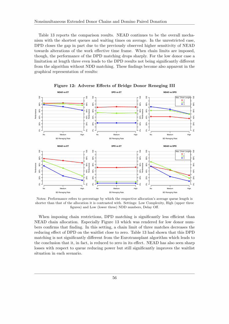
Nonsimultaneous Extended Donor Chains and Domino Paired Donation
Table 13 reports the comparison results. NEAD continues to be the overall mecha-nism with the shortest queues and waiting times on average. In the unrestricted case,DPD closes the gap in part due to the previously observed higher sensitivity of NEADtowards alterations of the work effective time frame. When chain limits are imposed,though, the performance of the DPD matching drops sharply. For the low donor case alimitation at length three even leads to the DPD results not being significantly differentfrom the algorithm without NDD matching. These findings become also apparent in thegraphical representation of results:
Figure 12: Adverse Effects of Bridge Donor Reneging III
NEAD vs ET
BD Reneging Rate
Perfo
rman
ce
! !!
!
!
!
! !
!
No Medium High
0%20
%40
%60
%80
%10
0
0%20
%40
%60
%80
%10
0
DPD vs ET
BD Reneging Rate
Perfo
rman
ce
!! !
! ! !
!! !
No Medium High
0%20
%40
%60
%80
%10
0
0%20
%40
%60
%80
%10
0
NEAD vs DPD
BD Reneging Rate
Perfo
rman
ce
! !
!
!
!
!
! !
!
No Medium High
0%20
%40
%60
%80
%10
0
0%20
%40
%60
%80
%10
0
!
!
!
Max. Chain Length!63
NEAD vs ET
BD Reneging Rate
Perfo
rman
ce
!
!
!
!
!
!
!
!
!
No Medium High
0%20
%40
%60
%80
%10
0
0%20
%40
%60
%80
%10
0
DPD vs ET
BD Reneging Rate
Perfo
rman
ce
! ! !
! ! !
! ! !
No Medium High
0%20
%40
%60
%80
%10
0
0%20
%40
%60
%80
%10
0
NEAD vs DPD
BD Reneging Rate
Perfo
rman
ce
!
!
!
!
!
!
!
!
!
No Medium High
0%20
%40
%60
%80
%10
0
0%20
%40
%60
%80
%10
0
!
!
!
Max. Chain Length!63
Notes: Performance refers to percentage by which the respective allocation’s average queue length isshorter than that of the allocation it is contrasted with. Settings: Low Complexity, High (upper three
figures) and Low (lower three) NDD numbers, Delay Off.
When imposing chain restrictions, DPD matching is significantly less efficient thanNEAD chain allocation. Especially Figure 13 which was rendered for low donor num-bers confirms that finding. In this setting, a chain limit of three matches decreases thereducing effect of DPD on the waitlist close to zero. Table 13 had shown that this DPDmatching is not significantly different from the Eurotransplant algorithm which leads tothe conclusion that it, in fact, is reduced to zero in its effect. NEAD has also seen sharplosses with respect to queue reducing power but still significantly improves the waitlistsituation in each scenario.
56
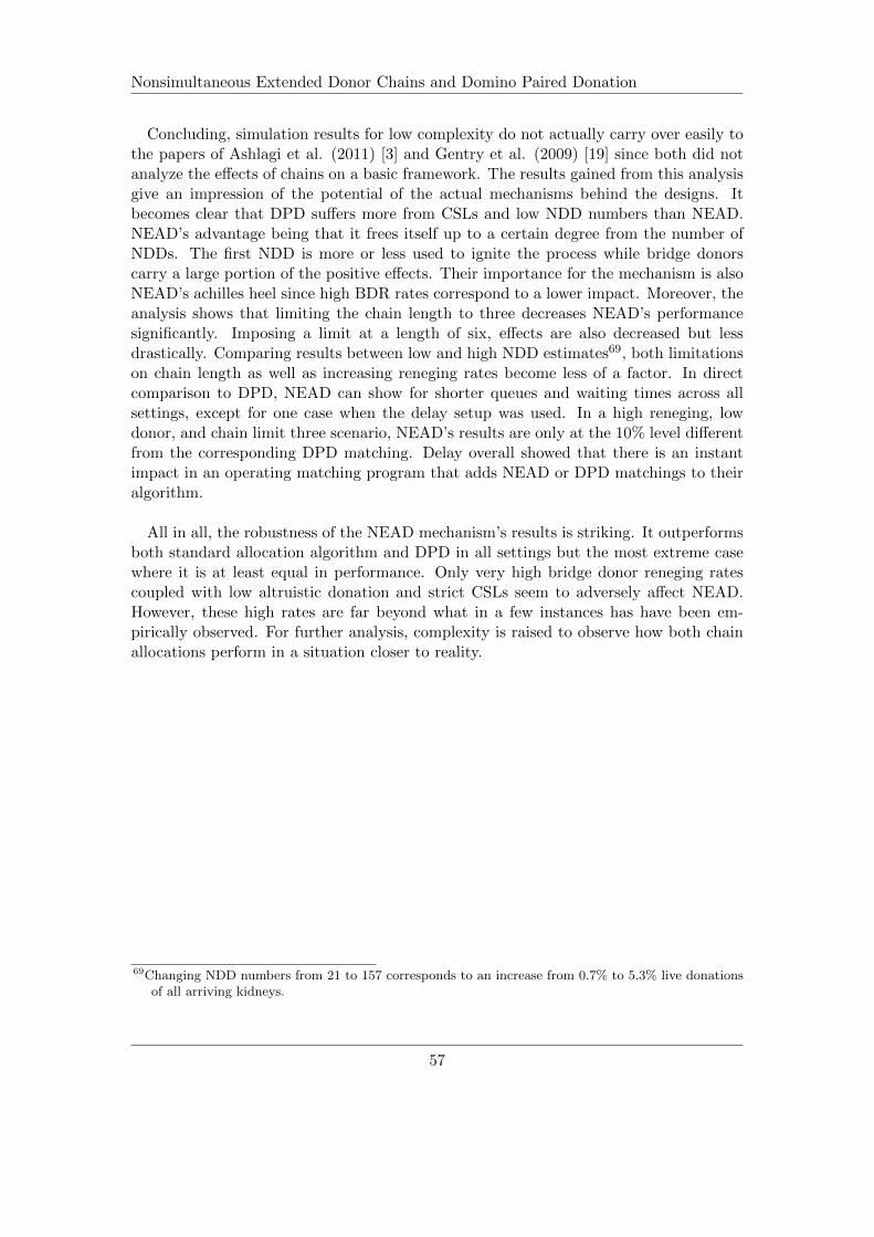
Nonsimultaneous Extended Donor Chains and Domino Paired Donation
Concluding, simulation results for low complexity do not actually carry over easily tothe papers of Ashlagi et al. (2011) [3] and Gentry et al. (2009) [19] since both did notanalyze the effects of chains on a basic framework. The results gained from this analysisgive an impression of the potential of the actual mechanisms behind the designs. Itbecomes clear that DPD suffers more from CSLs and low NDD numbers than NEAD.NEAD’s advantage being that it frees itself up to a certain degree from the number ofNDDs. The first NDD is more or less used to ignite the process while bridge donorscarry a large portion of the positive effects. Their importance for the mechanism is alsoNEAD’s achilles heel since high BDR rates correspond to a lower impact. Moreover, theanalysis shows that limiting the chain length to three decreases NEAD’s performancesignificantly. Imposing a limit at a length of six, effects are also decreased but lessdrastically. Comparing results between low and high NDD estimates69, both limitationson chain length as well as increasing reneging rates become less of a factor. In directcomparison to DPD, NEAD can show for shorter queues and waiting times across allsettings, except for one case when the delay setup was used. In a high reneging, lowdonor, and chain limit three scenario, NEAD’s results are only at the 10% level differentfrom the corresponding DPD matching. Delay overall showed that there is an instantimpact in an operating matching program that adds NEAD or DPD matchings to theiralgorithm.
All in all, the robustness of the NEAD mechanism’s results is striking. It outperformsboth standard allocation algorithm and DPD in all settings but the most extreme casewhere it is at least equal in performance. Only very high bridge donor reneging ratescoupled with low altruistic donation and strict CSLs seem to adversely affect NEAD.However, these high rates are far beyond what in a few instances has have been em-pirically observed. For further analysis, complexity is raised to observe how both chainallocations perform in a situation closer to reality.
69Changing NDD numbers from 21 to 157 corresponds to an increase from 0.7% to 5.3% live donationsof all arriving kidneys.
57

Nonsimultaneous Extended Donor Chains and Domino Paired Donation
8.4. High Complexity, Delay Off
The complexity option includes several features that were modeled after the currentlyemployed ETKAS.70 Among them, the possibility of rejection is introduced, which allowspatients to decline an offered organ for various reasons. The first two figures capture theeffects chain mechanisms have in a setting without any bridge donor reneging.
Figure 13: Queue Development VII
0 10 20 30 40 50
010
020
030
040
050
060
0
High NDD Numbers
Time (Weeks)
Wai
ting
List
Len
gth
LegendETDPD! DPD6DPD3
NEAD! NEAD6NEAD3
0 10 20 30 40 50
010
020
030
040
050
060
0
Low NDD Numbers
Time (Weeks)
Wai
ting
List
Len
gth
LegendETDPD! DPD6DPD3
NEAD! NEAD6NEAD3
Comparison of Queues over Time with Options: High Complexity, Delay Off, BDR Off
Notes: Average Queue Length over 52 weeks for NEAD, DPD, and ET allocations. BDR set to 0%.
While high complexity seems to have only mildly adverse effects on NEAD allocation,DPD is severely reduced in its performance. Especially when altruistic donor numbersare low, the difference in resulting average queue lengths between the two chain match-ings is striking. The following four figures give a first impression as to how sensitiveNEAD reacts in this setting towards increased bridge donor reneging rates.
It becomes apparent, that NEAD is far more sensitive to increased reneging thanin the low complexity setting. Especially, when comparing these sets of graphs withthe previous sets from the low complexity setup, NEAD reacts considerably stronger tothe raised complexity than DPD.The stark difference between low and high complexityespecially for the unlimited chain length setting could be due to a distinctly different dis-tribution of incompatible patient-donor pairs, which in turn limits NEAD in its efficiency.
70See Section 7 for a full description of added features.
58

Nonsimultaneous Extended Donor Chains and Domino Paired Donation
Figure 14: Queue Development VIII
0 10 20 30 40 50
010
020
030
040
050
060
070
0
High NDD Numbers
Time (Weeks)
Wai
ting
List
Len
gth
LegendETDPD! DPD6DPD3
NEAD! NEAD6NEAD3
0 10 20 30 40 50
010
020
030
040
050
060
0
Low NDD Numbers
Time (Weeks)W
aitin
g Li
st L
engt
h
LegendETDPD! DPD6DPD3
NEAD! NEAD6NEAD3
Comparison of Queues over Time with Options: High Complexity, Delay Off, BDR Medium
0 10 20 30 40 50
010
020
030
040
050
060
0
High NDD Numbers
Time (Weeks)
Wai
ting
List
Len
gth
LegendETDPD! DPD6DPD3
NEAD! NEAD6NEAD3
0 10 20 30 40 50
010
020
030
040
050
060
0
Low NDD Numbers
Time (Weeks)
Wai
ting
List
Len
gth
LegendETDPD! DPD6DPD3
NEAD! NEAD6NEAD3
Comparison of Queues over Time with Options: High Complexity, Delay Off, BDR High
Notes: Average Queue Length over 52 weeks for NEAD, DPD, and ET allocations. BDR set to 12.5%(upper two figures) and 25% (lower two).
The high complexity setting with its various options could have easily changed theoverall composition of blood types in the incompatible patient-donor pair pool. Thishypothesis can, however, not be answered by this analysis and is the subject of a wholenew set of analyses and therefore omitted. The blood type distribution of transplantedpatients, however, will be discussed at the end of this section together with additionalresults.
59

Nonsimultaneous Extended Donor Chains and Domino Paired Donation
Table 14: NEAD vs DPD III
NEADNo BDR Med BDR Hi BDR
H (∞) (6) (3) (∞) (6) (3) (∞) (6) (3)(∞) 0.619 0.591 0.484 0.331 0.305 0.15 0.168 0.086 0.003
∗∗∗†† ∗∗∗†† ∗∗∗†† ∗∗∗†† ∗∗∗†† ∗∗∗†† ∗∗∗†† ∗∗∗†† ††
(6) 0.627 0.612 0.501 0.356 0.332 0.182 0.198 0.122 0.039∗∗∗ ∗∗∗ ∗∗∗ ∗∗∗ ∗∗∗ ∗∗∗ ∗∗∗ ∗∗∗ ∗∗
(3) 0.64 0.617 0.525 0.376 0.353 0.204 0.224 0.149 0.068
LDN
∗∗∗†† ∗∗∗†† ∗∗∗†† ∗∗∗†† ∗∗∗†† ∗∗∗†† ∗∗∗†† ∗∗∗†† ∗∗∗††
(∞) 0.639 0.626 0.61 0.578 0.543 0.454 0.411 0.395 0.148∗∗∗ ∗∗∗ ∗∗∗ ∗∗∗ ∗∗∗ ∗∗∗ ∗∗∗ ∗∗∗† ∗∗∗
DPD
(6) 0.687 0.677 0.662 0.622 0.614 0.525 0.49 0.473 0.257∗∗∗ ∗∗∗ ∗∗∗ ∗∗∗ ∗∗∗ ∗∗∗ ∗∗∗ ∗∗∗† ∗∗∗
(3) 0.752 0.743 0.732 0.702 0.687 0.63 0.591 0.583 0.414
HDN
∗∗∗ ∗∗∗ ∗∗∗ ∗∗∗ ∗∗∗ ∗∗∗ ∗∗∗ ∗∗∗† ∗∗∗
Notes: NEAD(columns) is tested against DPD(rows) for high and low NDD numbers, e.g.NEAD with no CSL and no BDR against DPD with chain limit three. (†) indicates thatNEAD’s results are not normally distributed. (††) the same for DPD and (†††) says thatboth sets of results are not normally distributed. In either case, a Kolmogorov-Smirnovtest instead of a t test was used. Settings: High Complexity, Delay Off.
Following the makeup of the previous analyses, Table 14 reports the factors by whichthe resulting average queue of a NEAD matching differs from a DPD allocation. Com-parisons for same settings are done on the diagonal from top left to bottom right ineach three by three box. In the upper half, DPD and NEAD are compared in a lowNDD numbers setting and in the lower half for the high setting. For all combinations ofsettings, NEAD boasts better numbers than DPD, except one. For the high BDR, lowNDD numbers, and CSL three setting, NEAD performs not significantly different thana DPD allocation with unlimited chain length. All other comparisons confirm that dis-tributions of corresponding NEAD and DPD queues differ significantly. One result thatturns around compared with the low complexity setting is the impact of low donor num-bers. Previously, DPD was mostly affected by lowering the number of altruistic donors.Factors were smaller in the high NDDs than in the lower case, i.e. NEAD’s lead over theDPD allocation was reduced when NDD numbers were increased. In a complex scenario,NEAD even gains on DPD when NDD numbers are increased in most settings.71 Thatshows that DPD is more sensitive to the complexities observed in an actual waiting listthan NEAD which implies that the latter is the more robust mechanism. In Table 15NEAD and DPD are compared to the Eurotransplant non-chain algorithm for the highcomplexity setting.
71NEAD’s increase is significant at the 1% level, corresponding tables are reported in the appendix:Tables 27-30.
60

Nonsimultaneous Extended Donor Chains and Domino Paired Donation
Table 15: DPD and NEAD vs ET performance results III
Low Non Directed Donor Numbers
Chain Length Limit ∞ 6 3
NEAD DPD NEAD DPD NEAD DPD
No Avg. Q. 0.655 <0.01 0.098 <0.01 0.639 <0.01 0.072 <0.01 0.539 <0.01 0.036 0.02
Avg. WT. 0.717 <0.01 0.108 <0.01 0.7 <0.01 0.08 <0.01 0.587 <0.01 0.042 0.02
Med Avg. Q. 0.415 <0.01 0.094 <0.01 0.391 <0.01 0.07 <0.01 0.251 <0.01 0.036 0.01
Avg. WT. 0.444 <0.01 0.104 <0.01 0.419 <0.01 0.078 <0.01 0.272 <0.01 0.04 0.01
Hi Avg. Q. 0.259 <0.01 0.102 <0.01 0.207 <0.01 0.068 <0.01 0.124 <0.01 0.036 0.02
Avg. WT. 0.281 <0.01 0.112 <0.01 0.224 <0.01 0.074 <0.01 0.137 <0.01 0.041 0.01
High Non Directed Donor Numbers
Chain Length Limit ∞ 6 3
NEAD DPD NEAD DPD NEAD DPD
No Avg. Q. 0.811 <0.01 0.478 <0.01 0.809 <0.01 0.399 <0.01 0.798 <0.01 0.239 <0.01
Avg. WT. 0.881 <0.01 0.51 <0.01 0.88 <0.01 0.428 <0.01 0.869 <0.01 0.265 <0.01
Med Avg. Q. 0.776 <0.01 0.466 <0.01 0.768 <0.01 0.398 <0.01 0.718 <0.01 0.241 <0.01
Avg. WT. 0.844 <0.01 0.499 <0.01 0.835 <0.01 0.426 <0.01 0.781 <0.01 0.266 <0.01
Hi Avg. Q. 0.694 <0.01 0.464 <0.01 0.674 <0.01 0.409 <0.01 0.553 <0.01 0.241 <0.01
Avg. WT. 0.75 <0.01 0.495 <0.01 0.73 <0.01 0.44 <0.01 0.592 <0.01 0.267 <0.01
Notes: BD Reneging values No : Off; Med : Medium; Hi : High; in rows. Chain lengthlimitations ∞, 6, 3 in columns, further sorted by NEAD and DPD results. Avg. Q.:Length of average queue during the course of the simulation. Avg. WT.: Average waitingtime for patients who were transplanted. Options: Complexity High, Delay Off. Postednumbers refer to the factor by which the corresponding mechanism was faster or shorterthan the currently employed system. p values are reported after results in smaller fontsize for two sample t tests of the respective distribution against that of the correspondingEurotransplant simulation.
Irrespective of the raise in complexity, NEAD and DPD continue to have a measurablysignificant impact. Even when settings are meant to put the two chain mechanisms un-der the most pressure, both significantly reduce waiting time and length of the waitlist.The numbers slightly correct the impression gained from the first graphical analysis.NEAD continues to outperform DPD in this setting, too.
Table 24 (in the appendix) gives the results of a direct comparison between low andhigh complexity NEAD chains for the low NDD case. On the diagonal from top left tobottom right are the figures for comparisons of same setting results. For example, whenreneging is at the medium level and chains are limited to six matches, NEAD in thelow complexity setting produced on average 70.2% shorter queues. These nine directcomparisons proof that NEAD in the low complexity setting does perform considerablybetter. The only cases in which the two settings account for a similar distribution ofqueue lengths is when the low complexity NEAD is under more restrictive constraints.For example, when comparing the infinite CSL to the limit at length three for the noreneging case. In that situation results are not statistically distinguishable. That impliesthat a high complexity level is as constraining to the NEAD mechanism as lowering the
61

Nonsimultaneous Extended Donor Chains and Domino Paired Donation
chain limit from infinite to three.
When donor numbers are high (Table 23; appendix), the stark difference in resultsis reduced somewhat but not completely. By comparing matching settings it becomesclear that NEAD still suffers considerably from the introduction of organ rejection,HLA, Panel Reactive Antibodies (PRA) matching, and so on. When taking all resultsinto account, NEAD in the low complexity scenario boasts queues which are shorter by39.19%. When regarding only matching comparisons, i.e. results posted on the diago-nal, the queue length for the low complexity NEAD matching is 33.73% shorter. In thelow donor case, NEAD has 67.24% shorter queues in direct comparison and taking allpossible combinations into account, queue numbers are on average 88.15% lower.
Table 16: High vs low complexity: Comparison of performance I
g
NEAD DPD
(∞) (6) (3) (∞) (6) (3)
Low NDD No BDR -0.769 -0.626 -0.448 DPD -1.083
Med BDR -1.493 -0.702 -0.359 -0.562
Hi BDR -1.231 -0.298 -0.125 -0.172
High NDD No BDR -0.097 -0.101 -0.136 DPD -0.804
Med BDR -0.317 -0.282 -0.39 -0.114
Hi BDR -0.72 -0.52 -0.474 -0.031�
Notes: Comparison of performance in terms of average queue length between high and lowcomplexity. High complexity in columns. Numbers report by what factor an allocationis shorter than in the low complexity setting. A negative factor then implies that it is,in fact, longer. E.g. DPD in setting CSL∞ and high NDD numbers saw the length ofits average queue increase by 80.4%.’�’ marks the only not significant number from twosample t testing with H0 : ”No difference in means”. All others significant with p � 0.01.Options: Delay Off.
Table 16 compares the effects the increase from low to high complexity had for bothchain mechanisms. The table is set up to only use comparisons for matching scenarios.The upper row shows how NEAD and DPD changed in a low NDD scenario and thelower row how they did in the high NDD numbers case. Both mechanisms saw lesslosses when there were many altruistic donors. Only NEAD saw higher losses in thehigh reneging, CSL3,high donor scenario. Overall, NEAD has become more sensitiveto changes in the settings which leads to higher reductions of performance compared toDPD in many scenarios. However, neither mechanism deals consistently better with thehigh complexity than the other. Overall, complexity has a clear adverse effect for chain
62

Nonsimultaneous Extended Donor Chains and Domino Paired Donation
allocations. Taking previous results into account, NEAD still performs significantly bet-ter even though its queue reducing power is less substantial.
Figure 15: Adverse Effects of Bridge Donor Reneging III
NEAD vs ET
BD Reneging Rate
Perfo
rman
ce
!!
!
!
!
!
!
!
!
No Medium High
0%20
%40
%60
%80
%10
0
0%20
%40
%60
%80
%10
0
DPD vs ET
BD Reneging Rate
Perfo
rman
ce
! ! !
! ! !
! ! !
No Medium High
0%20
%40
%60
%80
%10
0
0%20
%40
%60
%80
%10
0
!
!
!
Max. Chain Length!63
NEAD vs DPD
BD Reneging Rate
Perfo
rman
ce !
!
!
!
!
!
!
!
!
No Medium High
0%20
%40
%60
%80
%10
0
0%20
%40
%60
%80
%10
0
NEAD vs ET
BD Reneging Rate
Perfo
rman
ce
!
!
!
!
!
!
!
!
!
No Medium High
0%20
%40
%60
%80
%10
0
0%20
%40
%60
%80
%10
0
DPD vs ET
BD Reneging Rate
Perfo
rman
ce
! ! !
! ! !! ! !
No Medium High
0%20
%40
%60
%80
%10
0
0%20
%40
%60
%80
%10
0
NEAD vs DPD
BD Reneging Rate
Perfo
rman
ce !
!
!
!
!
!
!
!
!
No Medium High
0%20
%40
%60
%80
%10
0
0%20
%40
%60
%80
%10
0
!
!
!
Max. Chain Length!63
Notes: Performance refers to percentage by which the respective allocation’s average queue length isshorter than that of the allocation it is contrasted with. Settings: High Complexity, High NDD
numbers (upper three figures) and Low NDD numbers (lower three figures), Delay Off.
The upper three figures make the results visible for the high donor case while thelower figures were created from the low donor results. Similarly to the low complexityscenario, NEAD is less sensitive to bridge donor reneging, variations in donor numbers,and stricter chain limits than DPD to the latter two. However, the difference in perfor-mance is significantly lower (at the 1% level).
All in all, introducing additional features to the simulation to approximate realitymore closely has affected NEAD more adversely than DPD and made it more sensitiveto changes in the setup. Nevertheless, NEAD still produces the better results in terms ofqueue length and waiting time compared to DPD. In the next step of analysis, the chainmechanisms are introduced into an operating allocation mechanism to analyze whetherthe impressive impact in the low complexity setting carries over.
63
Nonsimultaneous Extended Donor Chains and Domino Paired Donation
8.5. High Complexity, Delay On
Finally, the last case is presented which is modeled after the current Eurotransplantsituation in which there is no centralized chain matching mechanism. While this analysisis too limited to make accurate predictions, a good impression is gained as to whathappens, if a full scale chain mechanism is introduced. The gray, vertical line marks thepoint when NEAD and DPD were activated.
Figure 16: Queue Development IX
0 10 20 30 40 50
010
020
030
040
050
060
0
High NDD Numbers
Time (Weeks)
Wai
ting
List
Len
gth
LegendETDPD! DPD6DPD3
NEAD! NEAD6NEAD3
0 10 20 30 40 50
010
020
030
040
050
060
070
0
Low NDD Numbers
Time (Weeks)
Wai
ting
List
Len
gth
LegendETDPD! DPD6DPD3
NEAD! NEAD6NEAD3
Comparison of Queues over Time with Options: High Complexity, Delay On, BDR Off
0 10 20 30 40 50
010
020
030
040
050
060
070
0
High NDD Numbers
Time (Weeks)
Wai
ting
List
Len
gth
LegendETDPD! DPD6DPD3
NEAD! NEAD6NEAD3
0 10 20 30 40 50
010
020
030
040
050
060
0
Low NDD Numbers
Time (Weeks)
Wai
ting
List
Len
gth
LegendETDPD! DPD6DPD3
NEAD! NEAD6NEAD3
Comparison of Queues over Time with Options: High Complexity, Delay On, BDR Medium
Notes: Average Queue Length over 52 weeks for NEAD, DPD, and ET allocations. BDR set to 12.5%(lower two figures) and 0% (upper two).
64

Nonsimultaneous Extended Donor Chains and Domino Paired Donation
The first set of figures show a similar impact on the queue as in the low complexityscenario. However, in the low donor situation both allocation policies in all variationsseem to perform visibly worse than in the previous setting. When increasing BDR, theeffect especially on the NEAD matchings in low donor settings becomes apparent. Whilethe decline in performance is also obvious in the high donor case, it is clearly less stronglyaffected than in the scenario with less altruistic donors. From these first impressions, itseems as if the combination of high complexity, low donors, and less time to perform,made the NEAD allocation decisively more sensitive to changes in the renege rate.
Figure 17: Queue Development X
0 10 20 30 40 50
010
020
030
040
050
060
0
High NDD Numbers
Time (Weeks)
Wai
ting
List
Len
gth
LegendETDPD! DPD6DPD3
NEAD! NEAD6NEAD3
0 10 20 30 40 50
010
020
030
040
050
060
0
Low NDD Numbers
Time (Weeks)
Wai
ting
List
Len
gth
LegendETDPD! DPD6DPD3
NEAD! NEAD6NEAD3
Comparison of Queues over Time with Options: High Complexity, Delay On, BDR High
Notes: Average Queue Length over 52 weeks for NEAD, DPD, and ET allocations. BDR set to 25%.
Table 17 compares DPD to NEAD results and gives the factors by which NEAD isshorter than DPD in its average queues. The diagonal paths in each three by three boxdescribe the results when NEAD and DPD are confronted with the same settings. In thehigh donor scenario, NEAD’s average queue lengths are at least 10% shorter than thoseof DPD policies for each comparison of same settings. In the low donor case, NEADloses its edge in performance faster with increasing reneging rates. The chain lengththree, high reneging NEAD policy shows results that are only at the 10% level differentfrom DPD allocation in the same setting. In the setting without delay, it was shownthat NEAD lost some of its lead when complexity was high and donor numbers reduced.This effect is even increased in this scenario. DPD which was found to be very sensitiveto decreases in altruistic donation gains on NEAD in the high complexity setting whenless NDDsare available. Therefore, it is proven that NEAD becomes more sensitive tochanges in NDD numbers than DPD when complexity is high.
65

Nonsimultaneous Extended Donor Chains and Domino Paired Donation
Table 17: NEAD vs DPD IV
NEADNo BDR Med BDR Hi BDR
H (∞) (6) (3) (∞) (6) (3) (∞) (6) (3)(∞) 0.183 0.169 0.12 0.124 0.111 0.029 0.06 0.052 0.017
∗∗∗ ∗∗∗ ∗∗∗ ∗∗∗ ∗∗∗ ∗ ∗∗∗ ∗∗∗
(6) 0.174 0.184 0.119 0.125 0.112 0.029 0.061 0.048 0.013∗∗∗ ∗∗∗ ∗∗∗ ∗∗∗ ∗∗∗ ∗ ∗∗∗ ∗∗∗ .
(3) 0.179 0.175 0.135 0.129 0.117 0.034 0.063 0.055 0.018
LDN
∗∗∗ ∗∗∗ ∗∗∗ ∗∗∗ ∗∗∗ ∗∗ ∗∗∗ ∗∗∗ .
(∞) 0.256 0.224 0.201 0.202 0.22 0.133 0.161 0.122 0.022∗∗∗ ∗∗∗ ∗∗∗ ∗∗∗ ∗∗∗ ∗∗∗ ∗∗∗ ∗∗∗ ∗
DPD
(6) 0.26 0.224 0.194 0.184 0.232 0.136 0.166 0.122 0.023∗∗∗ ∗∗∗ ∗∗∗ ∗∗∗ ∗∗∗ ∗∗∗ ∗∗∗ ∗∗∗ ∗
(3) 0.333 0.304 0.277 0.265 0.299 0.24 0.252 0.216 0.126
HDN
∗∗∗ ∗∗∗ ∗∗∗ ∗∗∗ ∗∗∗ ∗∗∗ ∗∗∗ ∗∗∗ ∗∗∗
Notes: NEAD(columns) is tested against DPD(rows) for high and low NDD numbers, e.g.NEAD with no CSL and no BDR against DPD with chain limit three. (†) indicates thatNEAD’s results are not normally distributed. (††) the same for DPD and (†††) says thatboth sets of results are not normally distributed. In either case, a Kolmogorov-Smirnovtest instead of a t test was used. Settings: High Complexity, Delay On.
Table 17 adds the finding that with increased complexity and delay, NEAD starts toreact more sensitive to increases in bridge donor reneging in the low donor case. Thepreviously explained fact that in the delayed setting only half of the available NDDs areactually used for chains in combination with the increased reneging makes each NDDand each bridge donor more valuable to the functioning of the mechanism. However,while DPD policy in the low donor setting with chain limits of six or three is not signifi-cantly different from the basic algorithm anymore, NEAD still has the ability to shortenthe queue significantly. This implies that for the first time in the simulation, a chainmechanism does not have any effect on the length of the queue. DPD has no statisticallymeasurable effect on the waiting list unless it is allowed to match infinitely long chains.This adds to the proof that NEAD is by far more robust and reliable in its performance.
In the high donor scenario, NEAD is only marginally affected by increased chain lim-its. In the no reneging setting, a chain restriction at length three reduces the score bywhich NEAD’s queue is shorter than that of the standard algorithm by only 0.047 pointscompared to the unrestricted case. Even when increasing bridge donor reneging to 25%per instance, the difference in average queue length does not lower NEAD’s numbers bymore than 0.087 points.
66

Nonsimultaneous Extended Donor Chains and Domino Paired Donation
Table 18: DPD and NEAD vs ET performance results IV
Low Non Directed Donor Numbers
Chain Length Limit ∞ 6 3
NEAD DPD NEAD DPD NEAD DPD
No Avg. Q. 0.207 <0.01 0.03 0.03 0.202 <0.01 0.024 >0.1 0.144 <0.01 0.011 >0.1
Avg. WT. 0.22 <0.01 0.035 0.02 0.217 <0.01 0.028 >0.1 0.153 <0.01 0.013 >0.1
Med Avg. Q. 0.14 <0.01 0.034 0.02 0.129 <0.01 0.026 >0.1 0.07 <0.01 0.012 >0.1
Avg. WT. 0.152 <0.01 0.039 0.02 0.143 <0.01 0.029 0.1 0.077 <0.01 0.013 >0.1
Hi Avg. Q. 0.081 <0.01 0.033 0.04 0.07 <0.01 0.024 >0.1 0.042 0.01 0.013 >0.1
Avg. WT. 0.091 <0.01 0.037 0.03 0.078 <0.01 0.026 0.09 0.048 <0.01 0.015 >0.1
High Non Directed Donor Numbers
Chain Length Limit ∞ 6 3
NEAD DPD NEAD DPD NEAD DPD
No Avg. Q. 0.395 <0.01 0.208 <0.01 0.381 <0.01 0.165 <0.01 0.348 <0.01 0.091 <0.01
Avg. WT. 0.435 <0.01 0.228 <0.01 0.419 <0.01 0.182 <0.01 0.379 <0.01 0.106 <0.01
Med Avg. Q. 0.362 <0.01 0.2 <0.01 0.364 <0.01 0.172 <0.01 0.307 <0.01 0.089 <0.01
Avg. WT. 0.393 <0.01 0.221 <0.01 0.396 <0.01 0.191 <0.01 0.328 <0.01 0.104 <0.01
Hi Avg. Q. 0.317 <0.01 0.203 <0.01 0.298 <0.01 0.164 <0.01 0.23 <0.01 0.088 <0.01
Avg. WT. 0.345 <0.01 0.226 <0.01 0.322 <0.01 0.182 <0.01 0.247 <0.01 0.103 <0.01
Notes: BD Reneging values No : Off; Med : Medium; Hi : High; in rows. Chain lengthlimitations ∞, 6, 3 in columns, further sorted by NEAD and DPD results. Avg. Q.:Length of average queue during the course of the simulation. Avg. WT.: Average waitingtime for patients who were transplanted. Options: Complexity High, Delay On. Postednumbers refer to the factor by which the corresponding mechanism was faster or shorterthan the currently employed system. p values are reported after results in smaller fontsize for two sample t tests of the respective distribution against that of the correspondingEurotransplant simulation.
When making a direct comparison to similar settings in the low complexity scenario,both chain policies are reduced in their efficiency considerably. NEAD and DPD bothare less sensitive to increased complexity when CSL are rather restrictive. This impliesthat increases in complexity take away lots of matching possibilities that were otherwiseexplored in the unlimited settings. This is also in line with findings both by Ashlagiet al. (2011) [3] and Gentry et al. (2009) [19] who reported that the average chainwas at about three in the scenarios they analyzed. Complete results for comparisons oflow to high complexity settings for NEAD can be found in the appendix in Tables 27 - 30.
Table 19 offers results for said comparison for matching settings for both DPD andNEAD. Both mechanisms lose less performance when NDD numbers are high, exceptfor NEAD in the least restricted scenario. A tendency shows that DPD suffers less thanDPD. Only in the low NDD numbers case when CSL is infinite, NEAD has smaller rel-ative losses. Compared to the no delay scenario this tendency seems to even out whenboth mechanisms had more time to function.
67

Nonsimultaneous Extended Donor Chains and Domino Paired Donation
Table 19: High vs low complexity: Comparison of performance II
g
NEAD DPD
(∞) (6) (3) (∞) (6) (3)
Low NDD No BDR -0.302 -0.276 -0.209 DPD -0.5
Med BDR -0.436 -0.243 -0.224 -0.244
Hi BDR -0.415 -0.367 -0.271 -0.065
High NDD No BDR -0.559 -0.287 -0.138 DPD -0.447
Med BDR -0.56 -0.158 -0.138 -0.086
Hi BDR -0.521 -0.094 -0.031� -0.029�
Notes: � only not significant number. All other with p � 0.01Complexity Low, Delay On,Change in Performance Measure: Queue Length for Last Patient!
The last set of figures gives a graphical representation of the main findings of thissection. High donor numbers again can compensate for many and strict constraints.The effects of CSL, higher BDR, and especially low donor numbers are more destructiveto NEAD policies in a low donor scenario. However, NEAD still significantly reducesthe waiting lists. DPD on the other hand is even close to being neglectable in a lowNDD numbers setting. When compared to the currently used algorithm without chainmatching, there is no statistically significant difference in said scenario.
Figure 18: Adverse Effects of Bridge Donor Reneging IV
NEAD vs ET
BD Reneging Rate
Perfo
rman
ce
!
!
!
!
!
!
!
!
!
No Medium High
0%20
%40
%60
%80
%10
0
0%20
%40
%60
%80
%10
0
DPD vs ET
BD Reneging Rate
Perfo
rman
ce
! ! !
! ! !
! ! !
No Medium High
0%20
%40
%60
%80
%10
0
0%20
%40
%60
%80
%10
0
NEAD vs DPD
BD Reneging Rate
Perfo
rman
ce
!
!
!
!
!
!
!
!
!
No Medium High
0%20
%40
%60
%80
%10
0
0%20
%40
%60
%80
%10
0
!
!
!
Max. Chain Length!63
Notes: Performance refers to percentage by which the respective allocation’s average queue length isshorter than that of the allocation it is contrasted with. Settings: High Complexity, High NDD
numbers, Delay Off.
68

Nonsimultaneous Extended Donor Chains and Domino Paired Donation
Figure 19: Adverse Effects of Bridge Donor Reneging V
NEAD vs ET
BD Reneging Rate
Perfo
rman
ce
!
!
!
!
!
!
!
!
!
No Medium High
0%20
%40
%60
%80
%10
0
0%20
%40
%60
%80
%10
0
DPD vs ET
BD Reneging RatePe
rform
ance
! ! !
! ! !! ! !
No Medium High
0%20
%40
%60
%80
%10
0
0%20
%40
%60
%80
%10
0
NEAD vs DPD
BD Reneging Rate
Perfo
rman
ce
!
!
!
!
!
!
!
!
!
No Medium High
0%20
%40
%60
%80
%10
0
0%20
%40
%60
%80
%10
0
!
!
!
Max. Chain Length!63
Notes: Performance refers to percentage by which the respective allocation’s average queue length isshorter than that of the allocation it is contrasted with. Settings: High Complexity, Low NDD
numbers, Delay Off.
Concluding, both high complexity and delay have the adverse effect on chain poli-cies that were to be expected from the initial factor analysis. However, at least NEADcontinues to produce shorter queues and waiting times for patients in all settings, eventhough results become more modest than in the more basic setups. The most strikingare the influences donor numbers have on NEAD’s performance which were far less of afactor in low complexity settings.
69

Nonsimultaneous Extended Donor Chains and Domino Paired Donation
8.6. Additional Results
Before this section comes to an end and conclusions are drawn, some additional resultsthat were not in the focus of this analysis shall be reported. The analysis was almostexclusively concerned with average queue length. While this is highly correlated withboth waiting time and number of transplants, other data was also collected that bearssome meaning for the participants in the kidney market.
First, the distribution of O patients among transplanted patients shall be investigated.It was said before, that this distribution is of special interest since this group of patientshas the smallest pool of compatible donors. It was empirically observed that this factleads to relatively large concentrations of O patients in kidney exchange programs.72
These programs cannot compensate for this effect by size since they are mostly managedby single medical centers or schools and therefore comparably small. To counter thisdevelopment, those programs among them that introduced chain matching forbid ABdonors to become bridge donors since they are only matchable to the smallest popu-lation of all, namely patients also with blood type AB. This would very likely lead tolong waiting times for and perhaps subsequent reneging of the bridge donors and a fur-ther increasing share of O patients in the pool of remaining patients. While the lattermechanism, the removal of AB donors from the pool of admissible bridge donors, wasnot implemented for the presented work, the resulting effects on the distribution of Opatients among transplant recipients shall be shown. Results are reported for the highcomplexity setting since this is by assumption the most restrictive case and unbalanceddistributions should show the most in this setup.
Table 20: Frequency of O patients among transplanted patients
Low Donor Numbers High Donor Numbers ET BaseNEAD DPD NEAD DPD
No Med High No Med High(∞) 0.51 0.49 0.47 0.46 0.51 0.51 0.51 0.49 0.45 0.516(6) 0.51 0.49 0.47 0.46 0.51 0.51 0.51 0.49 ” ”(3) 0.51 0.47 0.46 0.45� 0.51 0.51 0.50 0.47 ” ”
Notes: Relative frequency of blood type O among all transplanted patients. Base refersto the distribution of blood type O among the whole waitlist. Options: High Complexity,Delay Off. ’�’ only not significant number (p � 0.1) when testing against associatedEurotransplant distribution. All others with p � 0.01
While Eurotransplant fails without its exact blood type matching procedure to ade-quately reproduce the base distribution, NEAD is fairly stable as long as donor numberare high and reneging not too high. Noticeably, NEAD’s resulting blood type distri-bution is more balanced than that of DPD while the previous analyses showed thatNEAD is almost always more effectively matching. All NEAD policies in all settingsdo result in more O patients being among the transplanted by percentage than in theDPD or current Eurotransplant allocation. Regarding the discussed finding that NEAD
72E.g. Montgomery et al. (2006) [31]
70

Nonsimultaneous Extended Donor Chains and Domino Paired Donation
matches more patients to transplants, the absolute value of O patients is even higherthan the differences in percentages suggest. One has to take these results with care,though. NEAD matched in most settings the majority of all patients. Therefore, theresulting ABO distribution might be due to the fact that NEAD simply used all avail-able patients which in turn recreates the base distribution. This can unfortunately notbe disproven. However, NEAD does match more blood type O patients in the mostrestrictive scenarios, too, in which far less patients are transplanted. Moreover, it mightnot be a sound counterargument to assume that NEAD posts more balanced blood typedistributions because it is so efficient. Following is a graphical representation of Table 20.
Figure 20: Distribution of Blood Type O Among Transplanted Patients
NEAD
BD Reneging
Shar
e of
tran
spla
nted
O p
atie
nts
No Medium High
44%
46%
48%
50%
52%
DPD
BD Reneging
Shar
e of
tran
spla
nted
O p
atie
nts
No Medium High
44%
46%
48%
50%
52%
Eurotransplant
BD RenegingSh
are
of tr
ansp
lant
ed O
pat
ient
s
No Medium High
44%
46%
48%
50%
52%
NEAD
BD Reneging
Shar
e of
tran
spla
nted
O p
atie
nts
No Medium High
44%
46%
48%
50%
52%
LegendLow C.:!63Hi C.:!63
DPD
BD Reneging
Shar
e of
tran
spla
nted
O p
atie
nts
No Medium High
44%
46%
48%
50%
52%
Eurotransplant
BD Reneging
Shar
e of
tran
spla
nted
O p
atie
nts
No Medium High
44%
46%
48%
50%
52%
Notes: Distribution of blood type O patients among transplant recipients. The red line indicates theirshare in the base distribution from which the queue is formed. The top three figures were calculated
for the low donor scenario whereas the lower three were done for the high donor case.
Another important feature of the resulting distribution of transplanted patients is thepercentage of live donations among the performed transplantations. Graft survival ofkidneys from live donors has been reported to be significantly better compared withcadaveric organ donations, as described earlier.73 While sheer number of possible trans-plants is one important argument favoring NEAD, the percentage of transplants thatinvolved a kidney donated from a live donor give an impression of the quality advantage
73Cf. Section 4.2.
71

Nonsimultaneous Extended Donor Chains and Domino Paired Donation
NEAD offers.
Table 21 Frequency of live donations among all transplantations
Low Donor Numbers High Donor NumbersNEAD DPD ET NEAD DPD ET
No Med High No Med High(∞) 0.29 0.14 0.06 0.01 0.01 0.39 0.34 0.24 0.04 0.05(6) 0.28 0.13 0.05 0.01 0.01 0.38 0.33 0.22 0.04 0.05(3) 0.24 0.08 0.03 0.01 0.01 0.38 0.29 0.17 0.05 0.05
Notes: Frequency of live donations among all transplantations. Numbers calculated asaverage values for low and high complexity with delay on and off. No, Med, Hi, refer toNo, Medium, and High BDR. (∞), (6), and (3) refer to CSL∞, CSL6, and CSL3. Alldistributions were significantly different from the corresponding Eurotransplant result atthe 1% level.
While the bridge donor concept that drives NEAD allocation has shown profoundresults regarding total transplant numbers, it is also well performing regarding qualityof transplants. A minimum of 3% in a low donor, high reneging, three patient matchinglimit scenario, and a maximum of 39% live transplants when all restrictions are liftedare striking. DPD in comparison has about one percent of all transplanted patientsprofiting from live donation in the low donor setting and about 4-5% in the high donorcase. The partly better numbers of Eurotransplant are understandable when recognizingthat Eurotransplant matches decisively less patients to organs overall which gives extraweight to each live donor in comparison to the more effective DPD allocation.
Another interesting statistic regarding NEAD concerns bridge donors and their behav-ior when waiting for a new match. In the two most restrictive settings, i.e. CSL at threematches and high reneging, 16.82 bridge donors reneged on average in the low donorscenario which corresponds to 49% of all activated bridge donors. For the high donorcase, 103.44 or 51% reneged. Of all activated associated donors in these two settings,about 29.5% had to wait for either a new suitable pair to arrive or until they decided torenege. The average waiting time for bridge donors that waited is at 1.05 (low donors)and 1.12 (high donors) time units which corresponds for the simulation to 7.3 (low NDDnumbers case) or about 8 days (high NDD numbers situation). These numbers are heav-ily relying on the high reneging rates. When reneging is switched off, bridge donors waiton average for 1.44 time units which corresponds to 10 days in the low NDD numbersetting and for 3.74 time units or 3 weeks and 5 days in a high donor scenario. Thesewaiting time are clearly shorter than what has been empirically observed. This may bemostly due to the fact that this simulation made use of the whole Eurotransplant systemand did not focus on small scale approaches which are perhaps closer to what is possiblein the short term. However, the simulation showed the potential effects a considerationof economic models for chain allocation would have.
Also noteworthy is the effect the introduction of willful rejection of organs had. Againfor the most restrictive scenarios, each patient that got transplanted for all three al-
72

Nonsimultaneous Extended Donor Chains and Domino Paired Donation
location policies rejected on average 0.06 kidneys which is a low number but fits theempirically observed behavior. This result stands for both low and high donor numberscases and high to medium to no reneging. On average, 99% of patients who rejected akidney at one point were transplanted later in the process by NEAD in the high donor,high reneging, short chain length scenario. In the same setting, DPD assigned 97.3% ofpatients who declined a kidney an organ in the end and Eurotransplant 95.4% of thesepatients. NEAD’s percentage results are significantly better than those of both DPDand Eurotransplant at the 1% level. In the low donor setting with otherwise unchangedrestrictions, NEAD is reduced to 96.5% but still significantly better (at the 1% level)than both DPD (95.8%) and Eurotransplant (95.4%). While this is a positive finding forthe NEAD algorithm, it has to be considered that NEAD also transplants significantlymore patients. The fact that almost all patients who rejected a kidney received one inthe end regardless might alter the patients’ behavior. Patients could become more proneto reject a mediocre match, anticipating the high probability to receive another offer.This learning effect has not been modeled since it has not been empirically observed orstudied. Furthermore the effect might be rather small since assuming that patients donot like to gamble facing lethal illnesses appears to be a sound hypothesis.
One particular finding by Ashlagi et al. (2011) [3] could not be reproduced. Theauthors argued in their paper that the number of highly sensitized patients among thosetransplanted was significantly higher in NEAD regimes than in DPD matchings. In thepresent work, simulation results show that for all three types of matching, average PRAdoes not differ between the different allocation algorithms and is consistently at about8% sensitization. Moreover, both NEAD and DPD failed to increase average number ofHLA matches between transplanted patients and their respective grafts. The assumedreason for that is the fact that all three mechanisms made use of the Eurotransplantscore system. Therefore, patients are ranked across the same criteria whether the offeredorgan stems from a cadaveric or live donor. It is highly questionable why different mech-anisms that use the same base distribution of patients and the same balancing criteriafor ranking should produce differently distributed results, especially when differences innumbers are small. Further analysis of this topic is not central to this paper’s approach,though, and hence omitted. The fact, however, seemed noteworthy and is therefore re-ported.
Finally, it has to be noted that some of the results are due to the omission of kidneypaired exchanges. In the literature, chains are always used in connection with kidneypaired donation. Kidney paired donation, however, leads to a considerable reduction ofthe pool of available patient-donor pairs (which is intended). Since this work focussedsolely on chain allocation, it must be mentioned that results would be considerably milderwhen a large part of patient-donor pairs was removed by cycle allocations. However, ten-dencies would not change since number of pairs was reduced for both algorithms equally.
Concluding, NEAD does produce matchings that are more favorable for blood typeO patients. Moreover, waiting times in large scale models appear to be shorter than for
73

Nonsimultaneous Extended Donor Chains and Domino Paired Donation
the smaller clearinghouses the literature has reported on so far. Furthermore, the highnumber of transplants realized by NEAD policies coupled with the comparably higherprobability to receive an organ regardless of a previous rejection might affect patientsbehavior when offered a kidney.
74
Nonsimultaneous Extended Donor Chains and Domino Paired Donation
9. Conclusion
This work has presented a currently discussed approach to increase efficiency in the heav-ily regulated market for kidney transplants without breaking its rules, i.e. introducingmoney which is deemed repugnant, and applied it on the current European allocationagency Eurotransplant and its algorithm.
Overall, the hypothesis presented in this thesis could be confirmed. The Nonsimulta-neous Extended Altruistic Donor (NEAD) allocation mechanism was shown to be bothmore efficient and robust in settings with varying complexity than the Domino PairedDonation (DPD) chain matching. In a low complexity setting, NEAD proved to be lesssensitive to alterations in the setup than DPD. With increased complexity, NEAD be-came more sensitive overall. Bridge Donor Reneging (BDR) had a less stark effect onNEAD as reported by Gentry et al. (2009) [19]. Especially noteworthy is that NEADbecame more sensitive towards changes in the numbers of altruistic donors than DPDwhen complexity was increased. Chain length limitations were shown to affect DPDmore adversely overall than NEAD which contradicts some of the results presented byAshlagi et al. (2011) [3]. However, all in all, results of Ashlagi et al. could be confirmedfor the large scale integrated model of the German waitlist. The low complexity settingsgave an impression how chain allocations generally perform and how that is affected bythe consecutive increase of complexity. Furthermore, the delayed integration of chainmatchings into the market showed the potential impact of those mechanisms on a al-ready operating system. Taking all findings into account, chain allocations do have ameasurably positive effect on the kidney market and NEADis more efficient regardingboth quantity and quality of transplants.
The simulation was subject to several simplifications and assumptions, though. Itwas not possible to work with the exact numbers since Eurotransplant was not able toprovide them in a timely fashion. Therefore, there is a possibility of a general distortionin the data. Moreover, numbers of Non Directed Donors (NDDs) had to be projectedfor Germany since there are legal obstacles preventing altruistic donation effectivelyconcealing the number of potential donors. Instead, two estimates were calculated andcompared during the analyses. Moreover, no valid German data on pairwise kidneyexchange for large scale markets was found. It was therefore estimated that about halfof all patients found a willing, yet incompatible donor. A rather harsh assumption isthe truthful participation of hospitals which was shown by Ashlagi and Roth (2011) [4]not to be a dominant strategy for them. Most problematic is probably that no fittingtheoretic model could be found since the model proposed in the market design literatureassumes binary preferences which is only true for the American market. Zenios’ (1998)[59] queueing theoretic model was build for an analysis of discrimination on the waitinglist and specifically not for chain mechanisms. Therefore a theoretic placement of thiswork was not fully possible. However, market design is increasingly concerned with thepractical side of the market which is not always fully representable in a theoretic frame-work.
75

Nonsimultaneous Extended Donor Chains and Domino Paired Donation
Further analyses are useful to determine effects of chain allocations that could not befully discussed in this work. Exact ABO matching and AB bridge donors are two con-cepts that were not fully integrated to prevent the results from being further distorted.However, it might be interesting to analyze chain mechanisms with this features espe-cially when actually considering the implementation of such a mechanism. Additionally,the effect of the higher matching rate for NEAD allocation might have an impact onthe behavior of patients. The hypothesis that highly increased chances for subsequenttransplantation might also increase the rate by which patient’s willingly decline offeredorgans seems interesting enough for further research.
Finally, this work has added a small puzzle piece to the overall picture. NEAD hasbeen proven to be more effective in maximizing the effect of altruistic donation. A fur-ther implementation requires theoretic and practical insights as to how to get hospitalsto fully cooperate, for example. In the future, market design will become more impor-tant for economists as practical and relevant problems for such markets as the one forkidneys need economists to solve them.
76

Nonsimultaneous Extended Donor Chains and Domino Paired Donation
References
[1] Abdulkadiroglu, Atila, Parag A. Pathak, and Alvin E. Roth (2005a), The New YorkCity High School Match, in: American Economic Review, Vol. 95, No. 2, pp. 364 -367.
[2] Abdulkadiroglu, Atila, Parag A. Pathak, Alvin E. Roth, and Tayfun Sonmez(2005b), The Boston Public School Match, in: American Economic Review, Vol.95, No. 2, pp. 368 - 371.
[3] Ashlagi, Itai, Duncan S. Gilchrist, Michael A. Rees, and Alvin E. Roth (2011),Nonsimultaneous Chains and Dominos in Kidney Paired Donation Revisited, in:American Journal of Transplantation, No. 11, pp. 984 - 994.
[4] Ashlagi, Itai and Alvin E. Roth (2011), Individual rationality and participation inlarge scale, multi-hospital kidney exchange, forthcoming.
[5] Avery, Christopher, Christine Jolls, Richard A. Posner, and Alvin E. Roth (2007),The Market for Federal Judicial Law Clerks, in: University of Chicago Law Review,Vol. 74, No. 2., pp. 448 - 486.
[6] Becker, Gary S. and Julio Jorge Elias (2007), Introducing Incentives in the Marketfor Live and Cadaveric Organ Donations, in: Journal of Economic Perspectives,Vol. 21, No. 3, pp. 3 - 24.
[7] Breyer, Friedrich and Hartmut Kliemt (2007), Der Mangel an Spenderorganen Ur-sachen und Loesungsmoeglichkeiten aus oekonomischer Sicht, in: Jahrbucher furNationalokonomie und Statistik, Vol. 227, No. 6, pp. 466 - 484.
[8] Cecka, J. Michael (2011), The UNOS renal transplant registry, in: Clinical Trans-plants 2001, pp. 1 - 18.
[9] Cohen, J. Wim (1969), The Single Server Queue, in: H. A. Lauwerier and W. T.Koiter (eds.), North-Holland Series in Applies Mathematics and Mechanics, Vol. 8,New York, NY., USA.
[10] Delmonico, Frank L. (2004), Exchanging kidneys - advances in living-donor trans-plantation, in: New England Journal for Medicine, Vol. 350, pp. 1812 - 1814.
[11] Edmonds, Jack (1965), Paths, Trees, and Flowers, in: Canadian Journal of Mathe-matics, No. 17, pp. 449 - 467.
[12] Erlang, Agner K. (1909), Sandsynlighetsregning og Telefonsamtaler, in: Nyttidsskrift for Matematik B, Vol. 20, pp. 33 - 40.
[13] Eurotransplant International Foundation (2011), Eurotransplant Manual - Chapter4: ET Kidney Allocation System (ETKAS), Version 1.8, Leiden, NL.
77
Nonsimultaneous Extended Donor Chains and Domino Paired Donation
[14] Fijter, Johan W. de (2010), Kidney allocation: where utility and fairness meet, in:Nephrology Dialysis Transplantation, Vol. 25, No. 6, pp. 1746 - 1749.
[15] Furrer, Reinhard, Douglas Nychka, and Stephen Sain (2010), fields: Tools for spatialdata. R package version 6.3., source: http://CRAN.R-project.org/package=fields
[16] Gale, David and Lloyd Shapley (1962), College Admissions and the Stability ofMarriage, in: American Mathematical Monthly, No. 69, pp. 9 - 15.
[17] Gallai, Tibor (1963), Kritische Graphen II, in: Magyar Tud. Akad. Mat., Vol. 8,pp. 373 - 395.
[18] Gallai, Tibor (1964), Maximale Systeme unabhangiger Kanten, in: Magyar Tud.Akad. Mat., Vol. 9, pp. 401 - 413.
[19] Gentry, Sommer E., Robert A. Montgomery, Bruce J. Swihart, and Dorry L. Segev(2009), The Roles of Dominos and Nonsimultaneous Chains in Kidney Paired Do-nation, in: American Jourmal of Transplantation, No. 9, pp. 1330 - 1336.
[20] Ghods, Ahad J.and Shekoufeh Savaj (2006), Iranian Model of Paid and RegulatedLiving Unrelated Kidney Donation, in: Clinical Journal of the American Society ofNephrology, Vol. 1, No. 6, pp. 1136 - 1145.
[21] Gjertson, David W. and J. Michael Cecka (2000), Living unrelated donor kidneytransplantation, in: Kidney International, Vol. 58, pp. 491 - 499.
[22] Gross, Donald and Carl M. Harris (1974), Fundamentals of Queueing Theory, FirstEdition, New York.
[23] Guba, Markus, Christian Graeb, Karl-Walter Jauch, and Edward K. Geissler (2004),Pro- and Anti-Cancer Effects of Immunosuppressive Agents Used in Organ Trans-plantation, in: Transplantation, Vol. 77, No. 12, pp. 1777 - 1782.
[24] Hatfield, John William and Scott Duke Kominers (2011), Multilateral Matching, in:Proceedings of the 12th ACM Conference on Electronic Commerce, pp. 337 - 338.
[25] Hatfield, John William and Paul R. Milgorm (2005), Matching with Contracts, in:American Economic Review, Vol. 95, No. 4, pp. 913 - 935.
[26] Klag, M. J., P. K. Whelton, B. L. Randall, J. D. Neaton, F. L. Brancati, C. E.Ford, N. B. Shulman, and J. Stamler (1996), Blood pressure and End Stage RenalDisease (ESRD) in men., in: New England Journal for Medicine, Vol. 334, No. 1,pp. 13 - 18.
[27] Klerk, Marry de, Karin M. Keizer, Frans H. J. Claas, Marin Witvliet, BernadetteJ. J. M. Haase-Kromwijk, and Willem Weimar (2005), The Dutch National LivingDonor Kidney Exchange Program, in: American Journal of Transplantation, Vol.5, No. 9, pp. 2302 - 2305.
78

Nonsimultaneous Extended Donor Chains and Domino Paired Donation
[28] Meester, Johan de, Guido G. Perslin, Thomas Wujciak, Gerhard Opelz, Yves Van-renterghem (1998), The New Eurotransplant Kidney Allocation System, in: Trans-plantation, Vol. 66, No. 9, pp. 1154 - 1159.
[29] Meier-Kreische, Herwig-Ulf, Friedrich K. Port, Akinlolu O. Ojo, Steven M. Rudich,Julie A. Hanson, Diane M. Cibrik, Alan B. Leichtman, and Bruce Kaplan (2000),Effect of waiting time on renal transplant outcome, in: Kidney International, Vol.58, pp. 1311 - 1317.
[30] Milgrom, Paul (2004) Putting Auction Theory to Work, Churchill Lectures in Eco-nomics, Cambridge: Cambridge University Press.
[31] Montgomery, Robert A., Sommer E. Gentry, William H. Marks, Daniel S. Warren,Janet Hiller, Julie Houp, Andrea A. Zachary, J. Keith Melancon, Warren R. Maley,Hamid Rabb, Christopher Simpkins, and Dorry L. Segev (2006), Domino pairedkidney donation: a strategy to make best use of live non-directed donation, in: TheLancet, No. 368, pp. 419 - 421.
[32] Muller, Carlheinz, Gerhard Ehninger, and Shraga F. Goldmann (2003), Gene andHaplotype Frequencies for the Loci Humane Leucocyte Antigene (HLA)-A, HLA-B,and HLA-DR Based on Over 13,000 German Blood Donors, in: Human Immunol-ogy, No. 64, pp. 137 - 151.
[33] Norris, James R. (1999), Markov Chains, Second Edition, Cambridge, UK.
[34] Oosterlee, Arie and Axel Rahmel (eds.) (2011), Eurotransplant Annual Report 2010,Eurotransplant International Foundation, Leiden, NL.
[35] Opelz, Gerhard (1997), Impact of HLA Compatibility on Survival of Kidney Trans-plants from Unrelated Live Donors, in: Transplantation, Vol. 64, No. 10, pp. 1473- 1475.
[36] Opelz, Gerhard (1998), HLA Compatibility and Kidney Grafts from Unrelated LiveDonors, in: Transplantation Proceedings, Vol. 30, No. 3, pp. 704 - 705.
[37] R Development Core Team (2011), R: A language and environment for statisti-cal computing, R Foundation for Statistical Computing, ISBN 3-900051-07-0, URLhttp://www.R-project.org/, Vienna, AT.
[38] Rapaport, Felix T. (1986), The case for a living emotionally related internationalkidney donor exchange registry, in: Transplantation Proceedings, Vol. 18, pp. 5 - 9.
[39] Rees, Michael A., Jonathan E. Kopke, Ronald S. Pelletier, Dorry L. Segev, MatthewE. Rutter, Alfredo J. Fabrega, Jeffrey Rogers, Oleh G. Pankewycz, Janet Hiller,Alvin E. Roth, Tuomas Sandholm, M. Utku Unver, and Robert A. Montgomery(2009), A Nonsimultaneous, Extended, Altruistic-Donor Chain, in: New EnglandJournal of Medicine, Vol. 360, pp. 1096 - 1101.
79

Nonsimultaneous Extended Donor Chains and Domino Paired Donation
[40] Ross, Lainie Friedman, David T. Rubin, Mark Siegler, Michelle A. Josephson, J.Richard Thistlethwaite Jr., and E. Steeve Woodle (1997), Ethics of a paired-kidney-exchange program, in: New England Journal of Medicine, Vol. 336, pp. 1752 - 1755.
[41] Roth, Alvin E. (1984), The Evolution of the Labor Market for Medical Interns andResidents: A Case Study in Game Theory, in: Journal of Political Economy, Vol.92, No. 6, pp. 991 - 1016.
[42] Roth, Alvin E. (1991), A Natural Experiment in the Organization of Entry LevelLabor Markets: Regional Markets for New Physicians and Surgeons in the U.K., in:American Economic Review, Vol. 81, No. 3, pp. 415 - 440.
[43] Roth, Alvin E. (2002), The Economist as Engineer: Game Theory, Experimenta-tion, and Computation as Tools for Design Economics, in: Econometrica, Vol. 70,No. 4, pp. 1341 - 1378.
[44] Roth, Alvin E. (2007), Repugnance as a Constraint on Markets, in: Journal ofEconomic Perspectives, Vol. 21, No. 3, pp. 37 - 58.
[45] Roth, Alvin E. (2008), What have we learned from market design?, Hahn Lecture,in: Economic Journal, Vol. 118, No. 527, pp. 285 - 310.
[46] Roth, Alvin E. and Elliott Peranson (1999), The Redesign of the Matching Mar-ket for American Physicians: Some Engineering Aspects of Economic Design, in:American Economic Review, Vol. 89, No. 4, pp. 748 - 780.
[47] Roth, Alvin E. and Marilda A. Sotomayor (1990), Two-Sided Matching: A Study inGame-Theoretic Modeling and Analysis, Econometric Society Monographs No. 18.,Cambridge, UK.
[48] Roth, Alvin E., Tayfun Sonmez, M. Utku Unver, Francis L. Delmonico, and Susan L.Saidman (2006), Utilizing List Exchange and Undirected Good Samaritan Donationthrough Chain Paired Kidney Exchanges, in: American Journal of Transplantation,Vol. 6, No.11, pp. 2694 - 2705.
[49] Roth, Alvin E., Tayfun Sonmez, and M. Utku Unver (2004), Kidney Exchange, in:Quarterly Journal of Economics, Vol. 119, No. 2, pp. 457 - 488.
[50] Roth, Alvin E., Tayfun Sonmez, and M. Utku Unver (2005a), Pairwise KidneyExchange, in: Journal of Economic Theory, No. 125, pp. 151 - 188.
[51] Roth, Alvin E., Tayfun Sonmez, and M. Utku Unver (2005b), A Kidney ExchangeClearinghouse in New England, in: American Economic Review, Vol. 95, No.2, pp.376 - 380.
[52] Roth, Alvin E., Tayfun Sonmez, and M. Utku Unver (2007), Efficient Kidney Ex-change: Coincidence of Wants in Markets with Compatibility-Based Preferences, in:American Economic Review, Vol. 97, No. 3, pp. 828 - 851.
80

Nonsimultaneous Extended Donor Chains and Domino Paired Donation
[53] Saidman, Susan L., Alvin E. Roth, Tayfun Sonmez, M. Utku Unver, and Francis L.Delmonico (2006), Increasing the Opportunity of Live Kidney Donation by Matchingfor Two and Three Way Exchanges, in: Transplantation, Vol. 81, No. 5, pp. 773 -782.
[54] Segev, Dorry L., Abimereki D. Muzaale, Brian S. Caffo, Shruti H. Mehta, Andrew L.Singer, Sarah E. Taranto, Maureen A. McBride, and Robert A. Montgomery (2010),Perioperative Mortality and Long-term Survival Following Live Kidney Donation,in: Journal of the American Medial Association,Vol. 303, No. 10, pp. 959 - 966.
[55] Shapley, Lloyd and Herbert Scarf (1974), On Cores and Indivisibility, in: Journalof Mathematical Economics, Vol. 1, No. 1, pp. 23 - 37.
[56] Sommerer, Claudia, Christian Morath, Joachim Andrassy, and Martin Zeier (2004),The long-term consequences of living-related or unrelated kidney donation, in:Nephrology, Dialysis, Transplantation, Vol. 19, Suppl. 4, pp. iv45 - iv47.
[57] Taylor, Howard M. and Samuel Karlin (1984), An Introduction to Stochastic Mod-eling, First Edition, Orlando, FL., USA.
[58] Witzke O., (2005), Uberkreuz-Lebendspende-Nierentransplantation in Deutschland,in: Deutsche Medizinische Wochenschrift, No. 130, pp. 2699 - 2702.
[59] Zenios, Stefanos A. (1998), Modeling the transplant waiting list: A queueing modelwith reneging, in: Queueing Systems, Vol. 31, pp. 239 - 251.
[60] Zenios, Stefanos A. and Xuanming Su (2004), Patient Choice in Kidney Allocation:The Role of the Queueing Discipline, in: Manufacturing & Service Operations Man-agement, Vol. 6, No. 4, pp. 280 - 301.
81

Nonsimultaneous Extended Donor Chains and Domino Paired Donation
A. Tables
The appendix contains additional tables that were omitted in the text to save space.The simulation, simulation libraries and subroutines, as well as all calculated results canbe found on the data disc that is distributed with this thesis or may alternatively berequested from the author via email: [email protected].
Table 22: HLA-ABDR Relative Frequencies
Allele Germany Eurotransplant Allele Germany Eurotransplant
A Alleles 40 0.07 0.070 0.01 0 41 0.01 0.011 0.16 0.16 42 < 0.01 < 0.012 0.3 0.29 46 < 0.01 < 0.013 0.15 0.16 47 < 0.01 < 0.019 0.11 0.12 48 < 0.01 < 0.0110 0.07 0.05 53 < 0.01 < 0.0111 0.05 0.05 59 < 0.01 < 0.0119 0.11 0.12 67 < 0.01 < 0.0128 0.04 0.04 70 < 0.01 < 0.0136 < 0.01 < 0.01 73 < 0.01 < 0.0143 < 0.01 < 0.01 78 0 < 0.0180 0 < 0.01 81 0 < 0.01203 0 < 0.01 82 0 < 0.01210 0 < 0.01 83 0 < 0.01
703 0 < 0.01B Alleles 2708 0 < 0.01
0 0.01 05 0.06 0.07 DR Alleles7 0.14 0.13 0 0.01 08 0.11 0.11 1 0.11 0.1112 0.13 0.13 3 0.11 0.1113 0.04 0.03 4 0.13 0.1414 0.02 0.02 7 0.13 0.1215 0.08 0.09 8 0.03 0.0316 0.04 0.04 9 0.01 0.0117 0.04 0.04 10 0.01 0.0118 0.05 0.05 11 0.12 0.1221 0.02 0.02 12 0.02 0.0222 0.02 0.02 13 0.12 0.1327 0.04 0.04 14 0.03 0.0335 0.1 0.1 15 0.16 0.1437 0.01 0.02 16 0.01 0.02
Notes: Data for Germany according to Muller et al. (2003) [32] and for Eurotransplantfrom the Eurotransplant Handbook Chapter 4 [13]. Numbers for Eurotransplant refer tothe whole Eurotransplant area, including Germany.
82

Nonsimultaneous Extended Donor Chains and Domino Paired Donation
Table 23: Distribution tests for NEAD in high vs low complexity settings I
High ComplexityNo BDR Med BDR Hi BDR
H (∞) (6) (3) (∞) (6) (3) (∞) (6) (3)(∞) -0.097 -0.137 -0.191 -0.322 -0.387 -0.671 -0.795 -0.855 -1.606
∗∗∗††† ∗∗∗††† ∗∗∗†† ∗∗∗†† ∗∗∗†† ∗∗∗†† ∗∗∗†† ∗∗∗†† ∗∗∗††
(6) -0.067 -0.101 -0.152 -0.279 -0.348 -0.621 -0.742 -0.798 -1.515∗∗∗† ∗∗∗† ∗∗∗ ∗∗∗ ∗∗∗ ∗∗∗ ∗∗∗ ∗∗∗ ∗∗∗
(3) -0.052 -0.083 -0.136 -0.261 -0.326 -0.598 -0.718 -0.777 -1.491
NoBDR
∗† ∗∗∗† ∗∗∗ ∗∗∗ ∗∗∗ ∗∗∗ ∗∗∗ ∗∗∗ ∗∗∗
(∞) -0.094 -0.13 -0.183 -0.317 -0.382 -0.665 -0.791 -0.844 -1.584∗∗∗† ∗∗∗† ∗∗∗ ∗∗∗ ∗∗∗ ∗∗∗ ∗∗∗ ∗∗∗ ∗∗∗
(6) -0.017 -0.049 -0.1 -0.228 -0.282 -0.55 -0.663 -0.716 -1.402!1 ∗∗† ∗∗∗ ∗∗∗ ∗∗∗ ∗∗∗ ∗∗∗ ∗∗∗ ∗∗∗
(3) 0.091 0.062 0.015 -0.1 -0.155 -0.39 -0.483 -0.541 -1.16
Low
Com
plexity
Med
BDR
∗∗∗† ∗∗† . ∗ ∗∗∗ ∗∗∗ ∗∗∗ ∗∗∗ ∗∗∗
(∞) -0.053 -0.087 -0.138 -0.268 -0.327 -0.604 -0.72 -0.777 -1.49∗† ∗∗∗† ∗∗∗ ∗∗∗ ∗∗∗ ∗∗∗ ∗∗∗ ∗∗∗ ∗∗∗
(6) 0.1 0.072 0.025 -0.087 -0.136 -0.371 -0.473 -0.52 -1.124∗∗∗† ∗∗∗† ∗ ∗ ∗∗∗ ∗∗∗ ∗∗∗ ∗∗∗ ∗∗∗
(3) 0.375 0.355 0.324 0.249 0.217 0.053 -0.022 -0.061 -0.474
HiBDR
∗∗∗† ∗∗∗† ∗∗∗ ∗∗∗ ∗∗∗ ∗∗ ∗∗∗
Notes: NEAD’s performance in a high complexity setting is tested against itself in a lowcomplexity setting, e.g. NEAD with no Chain Size Limit (CSL) and no BDR againstNEAD with chain limit three and medium BDR. (†) indicates that NEAD’s results in thehigh complexity setting are not normally distributed. (††) the same for NEAD in the lowcomplexity setting and (†††) says that both sets of results are not normally distributed. Ineither case, a Kolmogorov-Smirnov test instead of a t test was used. Settings: Delay Off,NDD Numbers High.
83

Nonsimultaneous Extended Donor Chains and Domino Paired Donation
Table 24: Distribution tests for NEAD in high vs low complexity settings II
High ComplexityNo BDR Med BDR Hi BDR
H (∞) (6) (3) (∞) (6) (3) (∞) (6) (3)(∞) -0.769 -0.868 -1.364 -2.022 -2.118 -2.877 -2.779 -3.118 -3.527
∗∗∗†† ∗∗∗†† ∗∗∗†† ∗∗∗†† ∗∗∗†† ∗∗∗†† ∗∗∗†† ∗∗∗†† ∗∗∗††
(6) -0.538 -0.626 -1.066 -1.643 -1.75 -2.392 -2.295 -2.624 -2.963∗∗∗†† ∗∗∗†† ∗∗∗†† ∗∗∗†† ∗∗∗†† ∗∗∗†† ∗∗∗†† ∗∗∗†† ∗∗∗††
(3) -0.08 -0.141 -0.448 -0.868 -0.931 -1.388 -1.316 -1.564 -1.796
NoBDR
∗∗∗ ∗∗∗ ∗∗∗ ∗∗∗ ∗∗∗ ∗∗∗ ∗∗∗
(∞) -0.425 -0.529 -0.917 -1.493 -1.564 -2.194 -2.109 -2.407 -2.717∗∗∗†† ∗∗∗†† ∗∗∗†† ∗∗∗†† ∗∗∗†† ∗∗∗†† ∗∗∗†† ∗∗∗†† ∗∗∗††
(6) 0.046 -0.006 -0.274 -0.649 -0.702 -1.1 -1.047 -1.243 -1.444∗∗∗ . ∗∗∗ ∗∗∗ ∗∗∗ ∗∗∗ ∗∗∗ ∗∗∗ ∗∗∗
(3) 0.381 0.344 0.174 -0.066 -0.103 -0.359 -0.329 -0.446 -0.586
Low
Com
plexity
Med
BDR
∗∗∗ ∗∗∗ ∗∗∗ . ∗∗∗ ∗∗∗ ∗∗∗ ∗∗∗
(∞) -0.029 -0.09 -0.385 -0.79 -0.857 -1.276 -1.231 -1.442 -1.665∗∗∗ ∗∗∗ ∗∗∗ ∗∗∗ ∗∗∗ ∗∗∗ ∗∗∗
(6) 0.447 0.419 0.256 0.046 0.021 -0.212 -0.192 -0.298 -0.425∗∗∗ ∗∗∗ ∗∗∗ ∗∗ ∗ ∗∗∗ ∗∗∗ ∗∗∗ ∗∗∗
(3) 0.561 0.537 0.417 0.247 0.224 0.038 0.065 -0.022 -0.125
HiBDR
∗∗∗ ∗∗∗ ∗∗∗ ∗∗∗ ∗∗∗ ∗∗ ∗∗∗ ∗∗∗
Notes: NEAD’s performance in a high complexity setting is tested against itself in a lowcomplexity setting, e.g. NEAD with no CSL and no BDR against NEAD with chain limitthree and medium BDR. (†) indicates that NEAD’s results in the high complexity settingare not normally distributed. (††) the same for NEAD in the low complexity settingand (†††) says that both sets of results are not normally distributed. In either case, aKolmogorov-Smirnov test instead of a t test was used. Settings: Delay Off, NDD NumbersLow.
84

Nonsimultaneous Extended Donor Chains and Domino Paired Donation
Table 25: Distribution tests for NEAD in high vs low complexity settings III
High ComplexityNo BDR Med BDR Hi BDR
H (∞) (6) (3) (∞) (6) (3) (∞) (6) (3)(∞) -0.302 -0.355 -0.411 -0.432 -0.371 -0.514 -0.46 -0.53 -0.704
∗∗∗ ∗∗∗ ∗∗∗ ∗∗∗ ∗∗∗ ∗∗∗ ∗∗∗ ∗∗∗ ∗∗∗
(6) -0.22 -0.276 -0.331 -0.345 -0.292 -0.421 -0.379 -0.441 -0.612∗∗∗ ∗∗∗ ∗∗∗ ∗∗∗ ∗∗∗ ∗∗∗ ∗∗∗ ∗∗∗ ∗∗∗
(3) -0.114 -0.164 -0.209 -0.231 -0.177 -0.301 -0.261 -0.322 -0.461
NoBDR
∗∗∗ ∗∗∗ ∗∗∗ ∗∗∗ ∗∗∗ ∗∗∗ ∗∗∗ ∗∗∗ ∗∗∗
(∞) -0.307 -0.361 -0.412 -0.436 -0.376 -0.513 -0.475 -0.538 -0.711∗∗∗ ∗∗∗ ∗∗∗ ∗∗∗ ∗∗∗ ∗∗∗ ∗∗∗ ∗∗∗ ∗∗∗
(6) -0.179 -0.234 -0.277 -0.295 -0.243 -0.372 -0.333 -0.392 -0.547∗∗∗ ∗∗∗ ∗∗∗ ∗∗∗ ∗∗∗ ∗∗∗ ∗∗∗ ∗∗∗ ∗∗∗
(3) -0.056 -0.104 -0.139 -0.159 -0.111 -0.224 -0.191 -0.246 -0.388
Low
Com
plexity
Med
BDR
∗∗∗ ∗∗∗ ∗∗∗ ∗∗∗ ∗∗∗ ∗∗∗ ∗∗∗ ∗∗∗
(∞) -0.255 -0.307 -0.355 -0.375 -0.324 -0.453 -0.415 -0.478 -0.645∗∗∗ ∗∗∗ ∗∗∗ ∗∗∗ ∗∗∗ ∗∗∗ ∗∗∗ ∗∗∗ ∗∗∗
(6) -0.162 -0.208 -0.249 -0.271 -0.219 -0.343 -0.304 -0.367 -0.522∗∗∗ ∗∗∗ ∗∗∗ ∗∗∗ ∗∗∗ ∗∗∗ ∗∗∗ ∗∗∗ ∗∗∗
(3) 0.031 -0.007 -0.045 -0.064 -0.019 -0.123 -0.089 -0.143 -0.271
HiBDR
∗∗ . ∗∗∗ ∗∗ ∗∗∗ ∗∗∗
Notes: NEAD’s performance in a high complexity setting is tested against itself in a lowcomplexity setting, e.g. NEAD with no CSL and no BDR against NEAD with chain limitthree and medium BDR. (†) indicates that NEAD’s results in the high complexity settingare not normally distributed. (††) the same for NEAD in the low complexity settingand (†††) says that both sets of results are not normally distributed. In either case, aKolmogorov-Smirnov test instead of a t test was used. Settings: Delay On, NDD NumbersLow.
85

Nonsimultaneous Extended Donor Chains and Domino Paired Donation
Table 26: Distribution tests for NEAD in high vs low complexity settings IV
High ComplexityNo BDR Med BDR Hi BDR
H (∞) (6) (3) (∞) (6) (3) (∞) (6) (3)(∞) -0.559 -0.569 -0.668 -0.654 -0.677 -0.838 -0.783 -0.794 -0.864
∗∗∗ ∗∗∗ ∗∗∗ ∗∗∗ ∗∗∗ ∗∗∗ ∗∗∗ ∗∗∗ ∗∗∗
(6) -0.274 -0.287 -0.364 -0.353 -0.371 -0.506 -0.457 -0.468 -0.526∗∗∗ ∗∗∗ ∗∗∗ ∗∗∗ ∗∗∗ ∗∗∗ ∗∗∗ ∗∗∗ ∗∗∗
(3) -0.066 -0.081 -0.138 -0.13 -0.152 -0.259 -0.216 -0.233 -0.272
NoBDR
. ∗∗∗ ∗∗∗ ∗∗∗ ∗∗∗ ∗∗∗ ∗∗∗ ∗∗∗
(∞) -0.467 -0.473 -0.568 -0.56 -0.59 -0.728 -0.672 -0.691 -0.76∗∗∗ ∗∗∗ ∗∗∗ ∗∗∗ ∗∗∗ ∗∗∗ ∗∗∗ ∗∗∗ ∗∗∗
(6) -0.067 -0.077 -0.138 -0.136 -0.158 -0.257 -0.215 -0.232 -0.274. . ∗∗∗ ∗∗∗ ∗∗∗ ∗∗∗ ∗∗∗ ∗∗∗ ∗∗∗
(3) 0.034 0.029 -0.024 -0.022 -0.04 -0.138 -0.097 -0.108 -0.152
Low
Com
plexity
Med
BDR
∗∗ ∗∗ ∗∗∗ ∗∗∗ ∗∗∗ ∗∗∗
(∞) -0.335 -0.347 -0.423 -0.425 -0.44 -0.573 -0.521 -0.534 -0.599∗∗∗ ∗∗∗ ∗∗∗ ∗∗∗ ∗∗∗ ∗∗∗ ∗∗∗ ∗∗∗ ∗∗∗
(6) 0.051 0.044 -0.015 -0.009 -0.026 -0.125 -0.087 -0.094 -0.138∗∗∗ ∗∗ ∗∗∗ ∗∗ ∗∗∗ ∗∗∗
(3) 0.135 0.13 0.079 0.084 0.069 -0.02 0.012 0.007 -0.031
HiBDR
∗∗∗ ∗∗∗ ∗∗∗ ∗∗∗ ∗∗∗ .
Notes: NEAD’s performance in a high complexity setting is tested against itself in a lowcomplexity setting, e.g. NEAD with no CSL and no BDR against NEAD with chain limitthree and medium BDR. (†) indicates that NEAD’s results in the high complexity settingare not normally distributed. (††) the same for NEAD in the low complexity settingand (†††) says that both sets of results are not normally distributed. In either case, aKolmogorov-Smirnov test instead of a t test was used. Settings: Delay On, NDD NumbersLow.
86

Nonsimultaneous Extended Donor Chains and Domino Paired Donation
Table 27: NEAD: Same setting distribution tests I
No BDR Med BDR Hi BDR
(∞) (6) (3) (∞) (6) (3) (∞) (6) (3)
(∞) - 11.49 55.58 19.1 75.07 153.44 8.84 4.24 45.63- ∗∗∗ ∗∗∗ ∗∗∗ ∗∗∗ ∗∗∗ ∗∗∗ ∗∗∗ ∗∗∗
(6) - 44.08 7.61 63.58 141.95 20.33 7.25 34.14- ∗∗∗ ∗∗∗ ∗∗∗ ∗∗∗ ∗∗∗ ∗∗∗ ∗∗∗
(3) - 36.47 19.5 97.86 64.41 51.33 9.95- ∗∗∗ ∗∗∗ ∗∗∗ ∗∗∗ ∗∗∗ ∗∗
(∞) - 55.97 134.33 27.94 14.86 26.52- ∗∗∗ ∗∗∗ ∗∗∗ ∗∗∗ ∗∗∗
(6) - 78.37 83.91 70.83 29.44- ∗∗∗ ∗∗∗ ∗∗∗ ∗∗∗
(3) - 162.28 149.2 107.81- ∗∗∗ ∗∗∗ ∗∗∗
(∞) - 13.08 54.47- ∗∗∗ ∗∗∗
(6) - 41.39- ∗∗∗
(3) --
Notes: This table describes the mean deviation between two different CSL and BDR set-tings in the same complexity and delay setup for NEAD allocations. Tested is the respec-tive row distribution against the column distribution and whether the two distributionsare similar(Ho : Equal distributions). T tests are employed since Kolmogorov-Smirnovtests verified the normality assumption for the respective results. NDD Numbers Low,Complexity Low, Delay Off.
87

Nonsimultaneous Extended Donor Chains and Domino Paired Donation
Table 28: NEAD: Same setting distribution tests II
No BDR Med BDR Hi BDR
(∞) (6) (3) (∞) (6) (3) (∞) (6) (3)
(∞) - =2.2 =3.51 =0.31 =5.92 16.05 70.3 194.5 254.9- ∗∗∗ ∗∗∗ ∗∗∗ ∗∗∗ ∗∗∗ ∗∗∗ ∗∗∗
(6) - 1.32 1.89 3.72 13.85 68.1 192.3 252.7- ∗∗∗ ∗∗∗ ∗∗∗ ∗∗∗ ∗∗∗ ∗∗∗ ∗∗∗
(3) - 3.21 2.41 12.53 66.78 190.98 251.39- ∗∗∗ ∗∗∗ ∗∗∗ ∗∗∗ ∗∗∗ ∗∗∗
(∞) - 5.62 15.74 69.99 194.19 254.6- ∗∗∗ ∗∗∗ ∗∗∗ ∗∗∗ ∗∗∗
(6) - 10.13 64.38 188.58 248.98- ∗∗∗ ∗∗∗ ∗∗∗ ∗∗∗
(3) - 54.25 178.45 238.85- ∗∗∗ ∗∗∗ ∗∗∗
(∞) - 124.2 184.6- ∗∗∗ ∗∗∗
(6) - 60.4- ∗
(3) --
Notes: This table describes the mean deviation between two different CSL and BDR set-tings in the same complexity and delay setup for NEAD allocations. Tested is the respec-tive row distribution against the column distribution and whether the two distributionsare similar(Ho : Equal distributions). T tests are employed since Kolmogorov-Smirnovtests verified the normality assumption for the respective results. NDD Numbers High,Complexity Low, Delay Off.
88
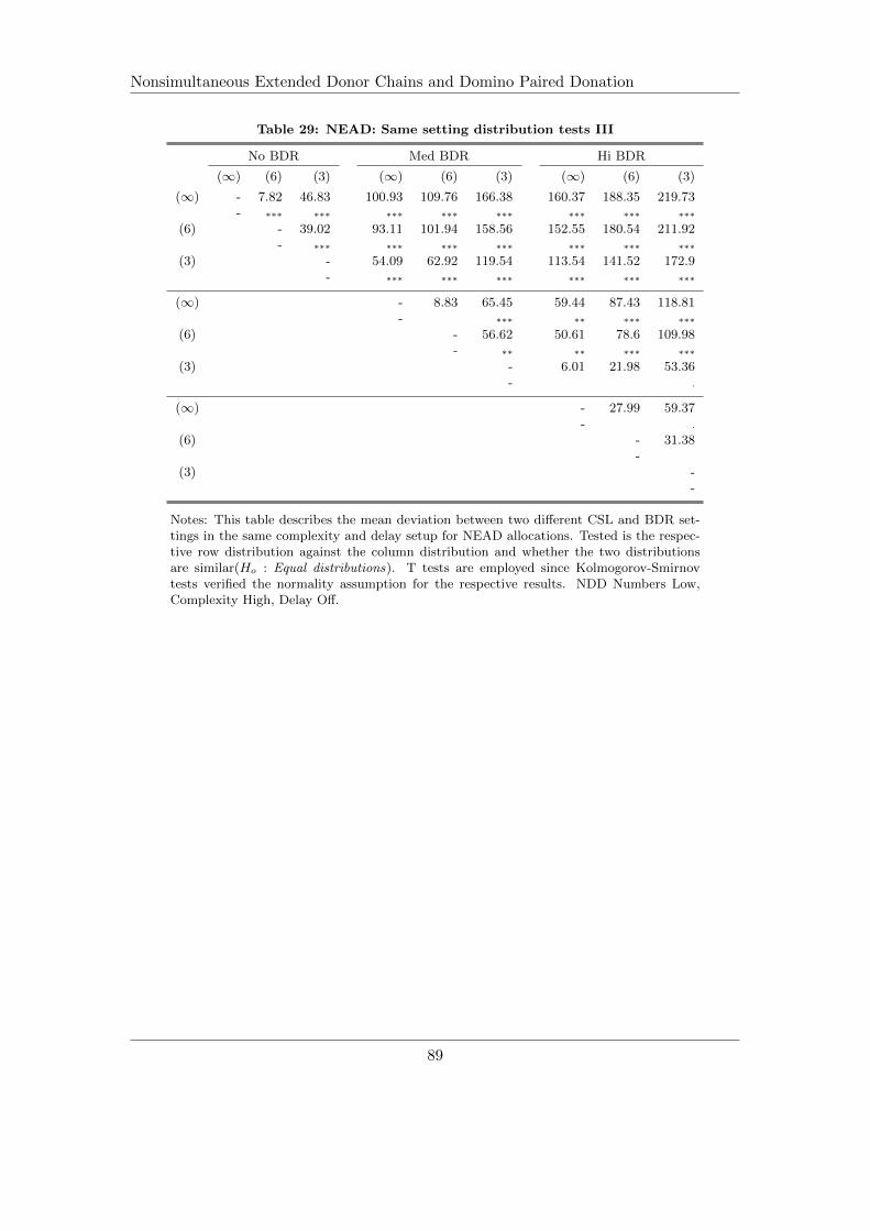
Nonsimultaneous Extended Donor Chains and Domino Paired Donation
Table 29: NEAD: Same setting distribution tests III
No BDR Med BDR Hi BDR
(∞) (6) (3) (∞) (6) (3) (∞) (6) (3)
(∞) - 7.82 46.83 100.93 109.76 166.38 160.37 188.35 219.73- ∗∗∗ ∗∗∗ ∗∗∗ ∗∗∗ ∗∗∗ ∗∗∗ ∗∗∗ ∗∗∗
(6) - 39.02 93.11 101.94 158.56 152.55 180.54 211.92- ∗∗∗ ∗∗∗ ∗∗∗ ∗∗∗ ∗∗∗ ∗∗∗ ∗∗∗
(3) - 54.09 62.92 119.54 113.54 141.52 172.9- ∗∗∗ ∗∗∗ ∗∗∗ ∗∗∗ ∗∗∗ ∗∗∗
(∞) - 8.83 65.45 59.44 87.43 118.81- ∗∗∗ ∗∗ ∗∗∗ ∗∗∗
(6) - 56.62 50.61 78.6 109.98- ∗∗ ∗∗ ∗∗∗ ∗∗∗
(3) - 6.01 21.98 53.36- .
(∞) - 27.99 59.37- .
(6) - 31.38-
(3) --
Notes: This table describes the mean deviation between two different CSL and BDR set-tings in the same complexity and delay setup for NEAD allocations. Tested is the respec-tive row distribution against the column distribution and whether the two distributionsare similar(Ho : Equal distributions). T tests are employed since Kolmogorov-Smirnovtests verified the normality assumption for the respective results. NDD Numbers Low,Complexity High, Delay Off.
89

Nonsimultaneous Extended Donor Chains and Domino Paired Donation
Table 30: NEAD: Same setting distribution tests IV
No BDR Med BDR Hi BDR
(∞) (6) (3) (∞) (6) (3) (∞) (6) (3)
(∞) - 2.4 =6.14 =15.52 =19.83 =39.7 =48.3 5=2.37 =10.04- ∗∗∗ ∗∗∗ ∗∗∗ ∗∗∗ ∗∗∗ ∗∗∗ ∗∗∗ ∗∗∗
(6) - 3.75 13.12 17.44 37.31 45.9 49.98 7.65- ∗∗∗ ∗∗∗ ∗∗∗ ∗∗∗ ∗∗∗ ∗∗∗ ∗∗∗
(3) - 9.38 13.69 33.56 42.15 46.23 3.9- ∗∗∗ ∗∗∗ ∗∗∗ ∗∗∗ ∗∗∗ ∗∗∗
(∞) - 4.31 24.18 32.78 36.85 5.48- ∗∗∗ ∗∗∗ ∗∗∗ ∗∗∗ ∗∗∗
(6) - 19.87 28.46 32.54 9.79- ∗∗∗ ∗∗∗ ∗∗∗ ∗∗∗
(3) - 8.59 12.67 29.66- ∗∗∗ ∗∗∗ ∗∗∗
(∞) - 4.07 38.25- ∗∗∗
(6) - 42.33- ∗∗∗
(3) --
Notes: This table describes the mean deviation between two different CSL and BDR set-tings in the same complexity and delay setup for NEAD allocations. Tested is the respec-tive row distribution against the column distribution and whether the two distributionsare similar(Ho : Equal distributions). T tests are employed since Kolmogorov-Smirnovtests verified the normality assumption for the respective results. NDD Numbers High,Complexity High, Delay Off.
90