normal forms, computer algebra and a problem of integrability of nonlinear odes
DESCRIPTION
Normal forms, computer algebra and a problem of integrability of nonlinear ODEs. Victor Edneral Moscow State University Russia Joint work with Alexander Bruno. Introduction Normal Form of a Nonlinear System Euler – Poisson Equations - PowerPoint PPT PresentationTRANSCRIPT
Normal forms, computer algebra and a problem of integrability of
nonlinear ODEs
Victor Edneral
Moscow State University
Russia
Joint work with Alexander Bruno

CADE-2007, February 20-23, Turku, Finland2
• Introduction• Normal Form of a Nonlinear System• Euler – Poisson Equations• Normal Form of the Euler – Poisson Equations in
Resonance• Structure of Integrals of the System• Necessary Conditions for Existence of Additional
Integrals• Calculation of the Normal Form of the Euler – Poisson
Equations• Conclusions

CADE-2007, February 20-23, Turku, Finland3
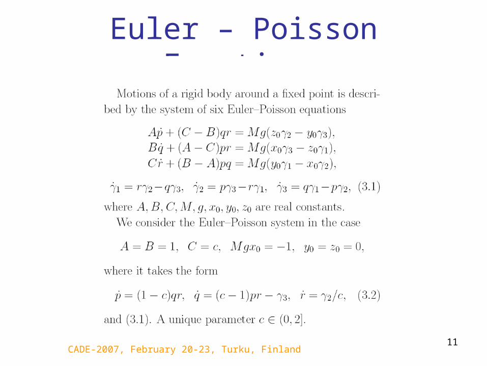
IntroductionHere, we study the connection between coefficients of normal forms and integrability of the system. For this purpose, we compute normal forms of the Euler – Poisson equations, which describe the motion of a rigid body with a fixed point. This is an autonomous sixth-order system.
A lot of books and papers are devoted to integrable systems and to methods for searching for such systems. A.D. Bruno noted that all normal forms of integrable systems are degenerated, so it is interesting to search domains with a such degeneration [Bruno, 2005].
The first attempt to calculate the normal form of the Euler – Poisson system was made in [Starzhinsky, 1977]. However, without computer algebra tools, he was unable to calculate a sufficient number of terms. We use a program for analytical computation of the normal form [V. Edneral, R. Khanin, 2003]. This is a modification of the LISP based package NORT for the MATHEMATICA system. The NORT package [Edneral, 1998] has been designed for the REDUCE system.

CADE-2007, February 20-23, Turku, Finland5
Normal Form of a Nonlinear System
Consider the system of order n
in a neighborhood of the stationary point X = 0 under the assumption that the vector function Φ(X) is analytical at the point X = 0 and its Taylor expansion contains no constant and linear terms.
(1.1)

CADE-2007, February 20-23, Turku, Finland6

CADE-2007, February 20-23, Turku, Finland7
CADE-2007, February 20-23, Turku, Finland8
CADE-2007, February 20-23, Turku, Finland9

CADE-2007, February 20-23, Turku, Finland10
CADE-2007, February 20-23, Turku, Finland11
Euler – Poisson Equations

CADE-2007, February 20-23, Turku, Finland12

CADE-2007, February 20-23, Turku, Finland13
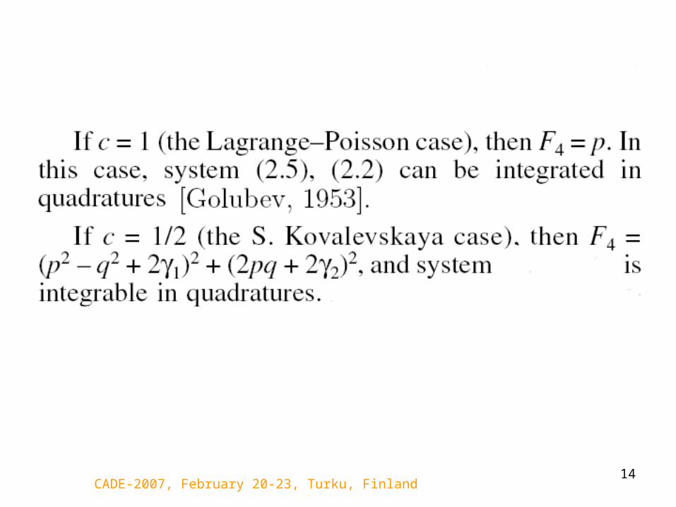
CADE-2007, February 20-23, Turku, Finland14

CADE-2007, February 20-23, Turku, Finland15
Has the system additional local integrals?
CADE-2007, February 20-23, Turku, Finland16
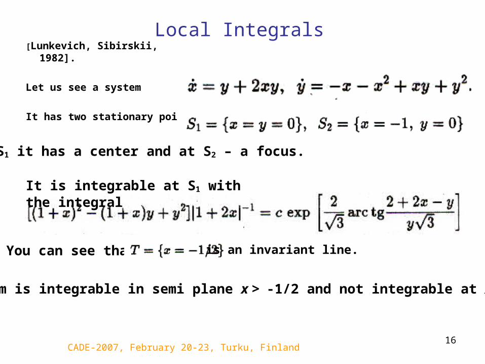
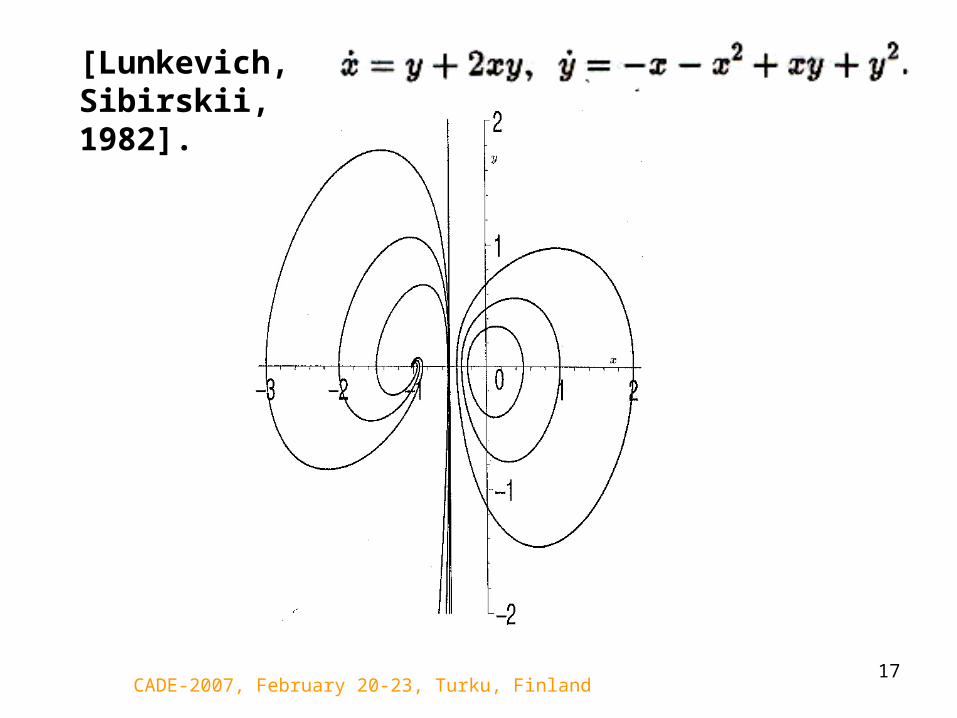
Local Integrals[Lunkevich, Sibirskii, 1982].
Let us see a system
It has two stationary points
At S1 it has a center and at S2 – a focus.
It is integrable at S1 with the integral
You can see that
The system is integrable in semi plane x > -1/2 and not integrable at x < -1/2.
is an invariant line.
CADE-2007, February 20-23, Turku, Finland17
[Lunkevich, Sibirskii, 1982].

CADE-2007, February 20-23, Turku, Finland18
CADE-2007, February 20-23, Turku, Finland19

CADE-2007, February 20-23, Turku, Finland20
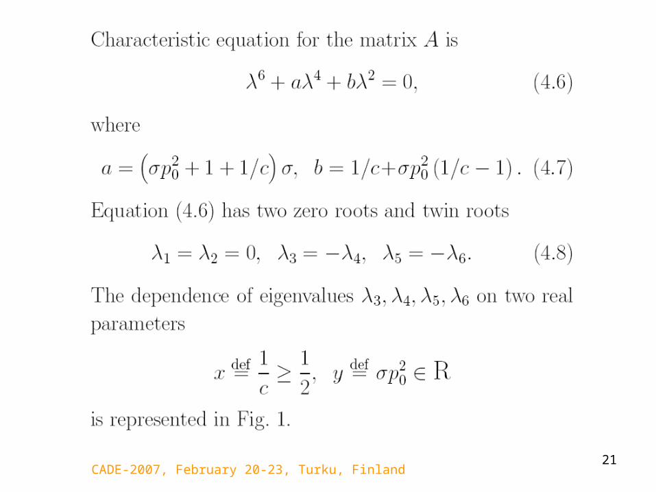
CADE-2007, February 20-23, Turku, Finland21

CADE-2007, February 20-23, Turku, Finland22
D2 D4
D1
D5 D3
C2 R +
R –
C3C1
(x0,y0)
Fig. 1
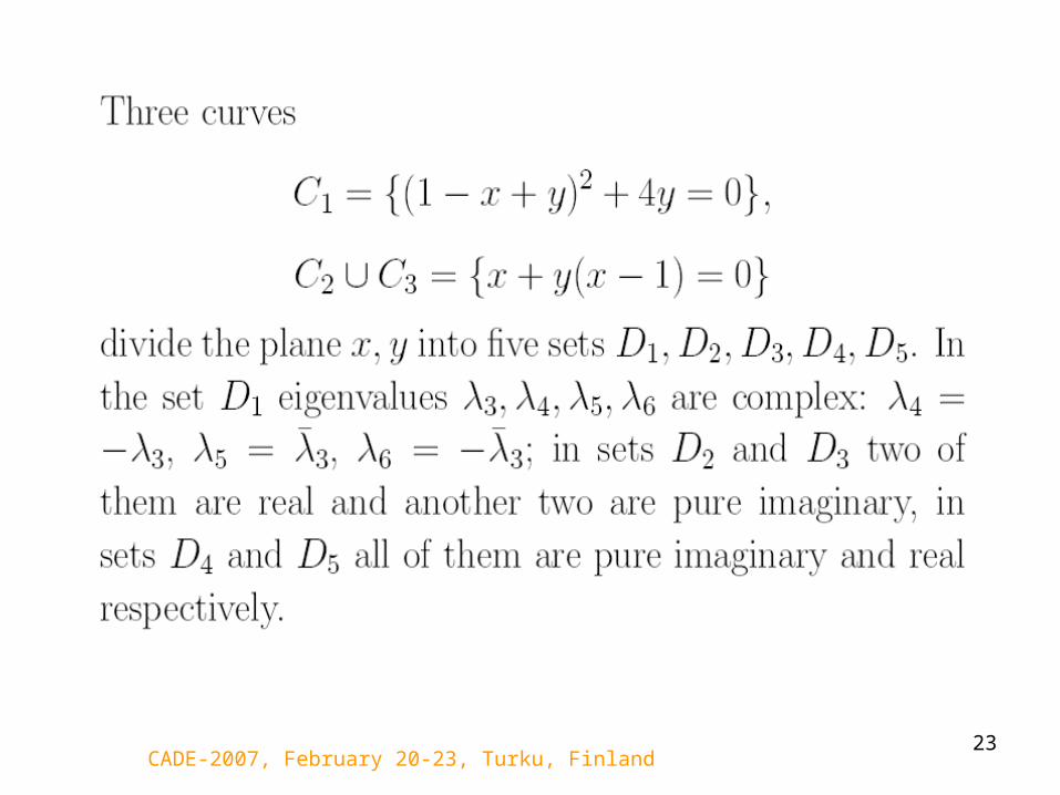
CADE-2007, February 20-23, Turku, Finland23

CADE-2007, February 20-23, Turku, Finland24

CADE-2007, February 20-23, Turku, Finland25
CADE-2007, February 20-23, Turku, Finland26
CADE-2007, February 20-23, Turku, Finland27

CADE-2007, February 20-23, Turku, Finland28
CADE-2007, February 20-23, Turku, Finland29
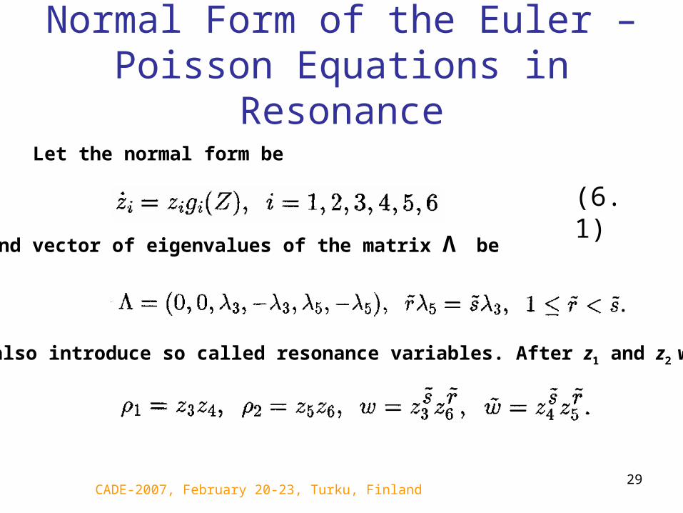
Normal Form of the Euler – Poisson Equations in Resonance
Let the normal form be
and vector of eigenvalues of the matrix Λ be
Let also introduce so called resonance variables. After z1 and z2 we have
(6.1)

CADE-2007, February 20-23, Turku, Finland30
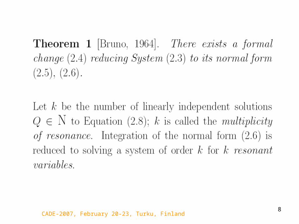
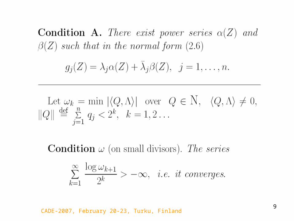
Lemm 1 [Bruno, 2005].At the resonance in the normal form
where
are power series in
At this start from free terms but
– from linear terms.
CADE-2007, February 20-23, Turku, Finland31
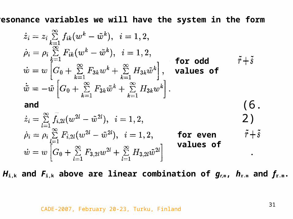
In resonance variables we will have the system in the form
for odd values of
and
for even values of
.
G0, Hi,k and Fi,k above are linear combination of gr,m, hr.m and fr.m.
(6.2)

CADE-2007, February 20-23, Turku, Finland32
Structure of Integrals of the SystemAs it was shown in [Bruno, 1995] an expansion of the first integral of normal form
contains only resonance variables with the property
Thus the first integral can be written as power series
where a0, am and bm are power series in z1, z2, ρ1, ρ2.
CADE-2007, February 20-23, Turku, Finland33
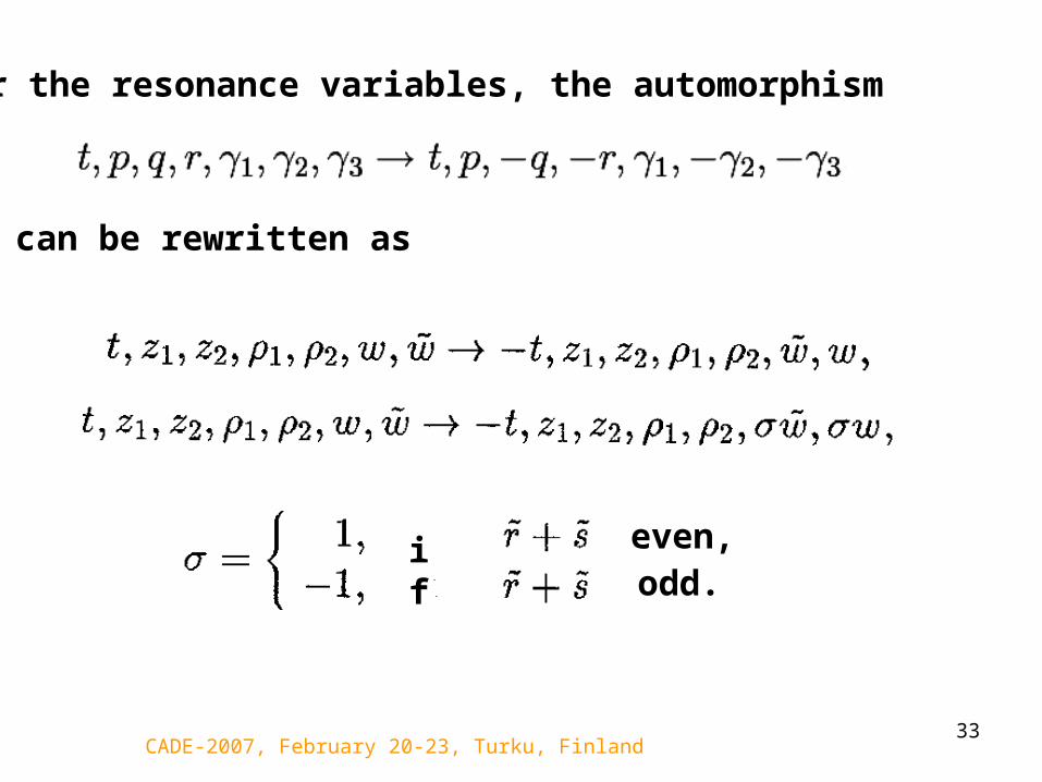
For the resonance variables, the automorphism
if
can be rewritten as
even,odd.

CADE-2007, February 20-23, Turku, Finland34
If is odd then the integral A will be
Then we have am = bm and the integral is
(7.1)

CADE-2007, February 20-23, Turku, Finland35
Necessary Conditions for Existence of Additional Integrals
From the definition, the derivation in time of any first integralalong the system should be zero, i.e.
CADE-2007, February 20-23, Turku, Finland36
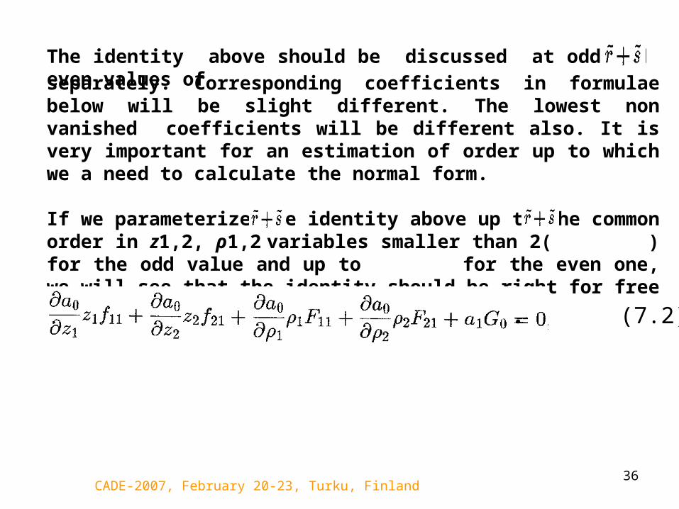
The identity above should be discussed at odd and even values of
separately. Corresponding coefficients in formulae below will be slight different. The lowest non vanished coefficients will be different also. It is very important for an estimation of order up to which we a need to calculate the normal form.
If we parameterize the identity above up to the common order in z1,2, ρ1,2 variables smaller than 2( ) for the odd value and up to for the even one, we will see that the identity should be right for free and linear in the common order
. (7.2)
CADE-2007, February 20-23, Turku, Finland37
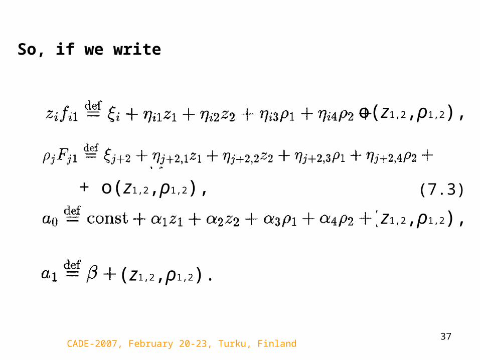
So, if we write
o(z1,2,ρ1,2),
O(z1,2,ρ1,2).
(7.3)
o(z1,2,ρ1,2),
+ o(z1,2,ρ1,2),

CADE-2007, February 20-23, Turku, Finland38
then the equation for the free term has the form
Here the vector Ξ ≡ {ξi} can be calculated from the normal form. It will be a function of parameters of the system. The vector α ≡ {αi} defines a0.
If you know the first integrals of the system, you can calculate the corresponding α ≡ {αi} for each integral separately.
(A)
If Ξ ≠ 0 then equation (A) has three dimensional set of solutionsα, so only three integrals can be independent.
CADE-2007, February 20-23, Turku, Finland39
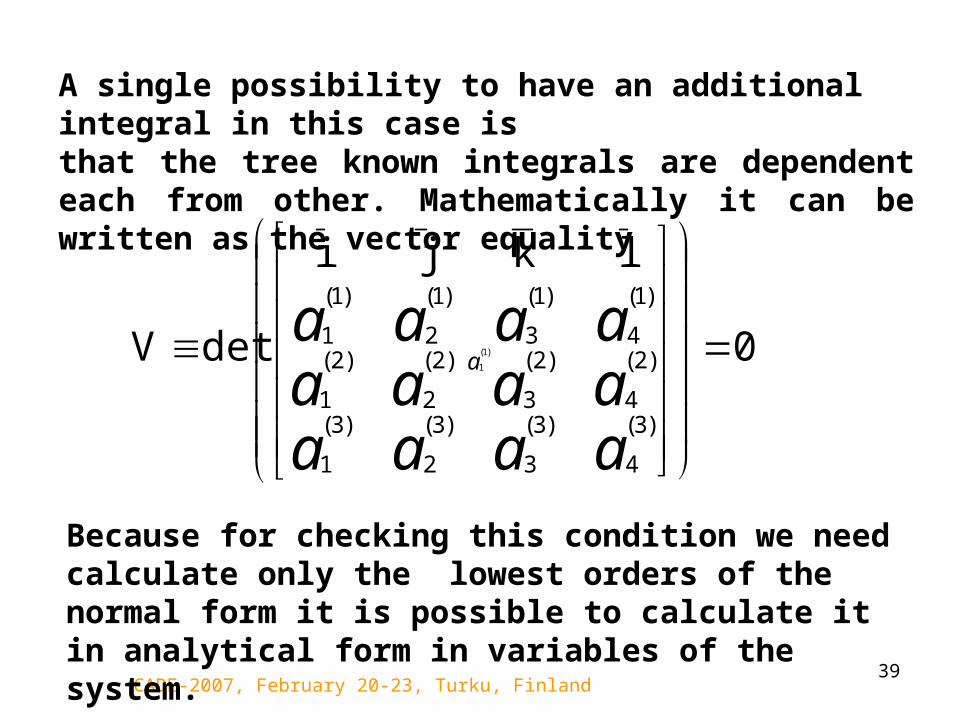
A single possibility to have an additional integral in this case is that the tree known integrals are dependent each from other. Mathematically it can be written as the vector equality
0
lkji
detV
)3(
4
)3(
3
)3(
2
)3(
1
)2(
4
)2(
3
)2(
2
)2(
1
)1(
4
)1(
3
)1(
2
)1(
1
aaaaaaaaaaaa
Because for checking this condition we need calculate only the lowest orders of the normal form it is possible to calculate it in analytical form in variables of the system.
a)1(
1
CADE-2007, February 20-23, Turku, Finland40
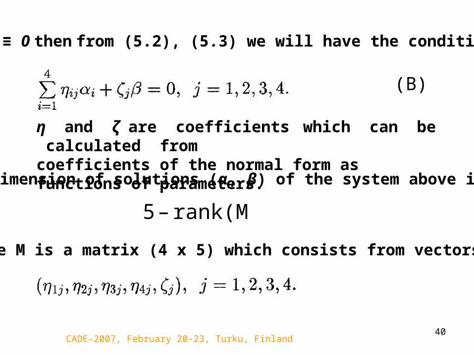
If Ξ ≡ 0 then from (5.2), (5.3) we will have the condition
(B)
The dimension of solutions (α, β) of the system above is
rank(M),– 5
where M is a matrix (4 x 5) which consists from vectors
η and ζ are coefficients which can be calculated fromcoefficients of the normal form as functions of parameters.
CADE-2007, February 20-23, Turku, Finland41
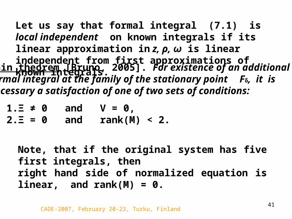
Let us say that formal integral (7.1) is local independent on known integrals if its linear approximation in z, ρ, ω is linear independent from first approximations of known integrals.
Main theorem [Bruno, 2005]. For existence of an additional formal integral at the family of the stationary point Fδ, it is necessary a satisfaction of one of two sets of conditions:
1. Ξ ≠ 0 and V = 0,2. Ξ = 0 and rank(M) < 2.
Note, that if the original system has five first integrals, thenright hand side of normalized equation is linear, and rank(M) = 0.
CADE-2007, February 20-23, Turku, Finland42
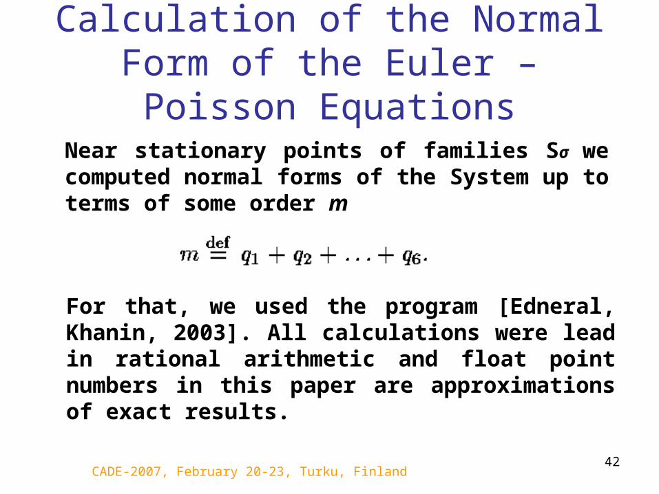
Calculation of the Normal Form of the Euler – Poisson Equations
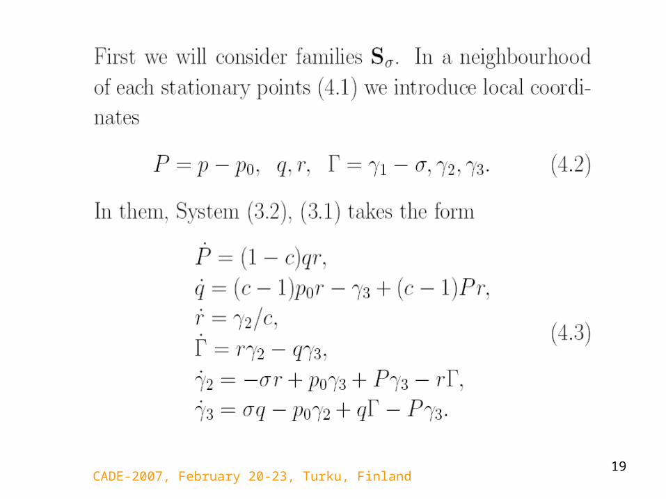
Near stationary points of families Sσ we computed normal forms of the System up to terms of some order m
For that, we used the program [Edneral, Khanin, 2003]. All calculations were lead in rational arithmetic and float point numbers in this paper are approximations of exact results.
CADE-2007, February 20-23, Turku, Finland43
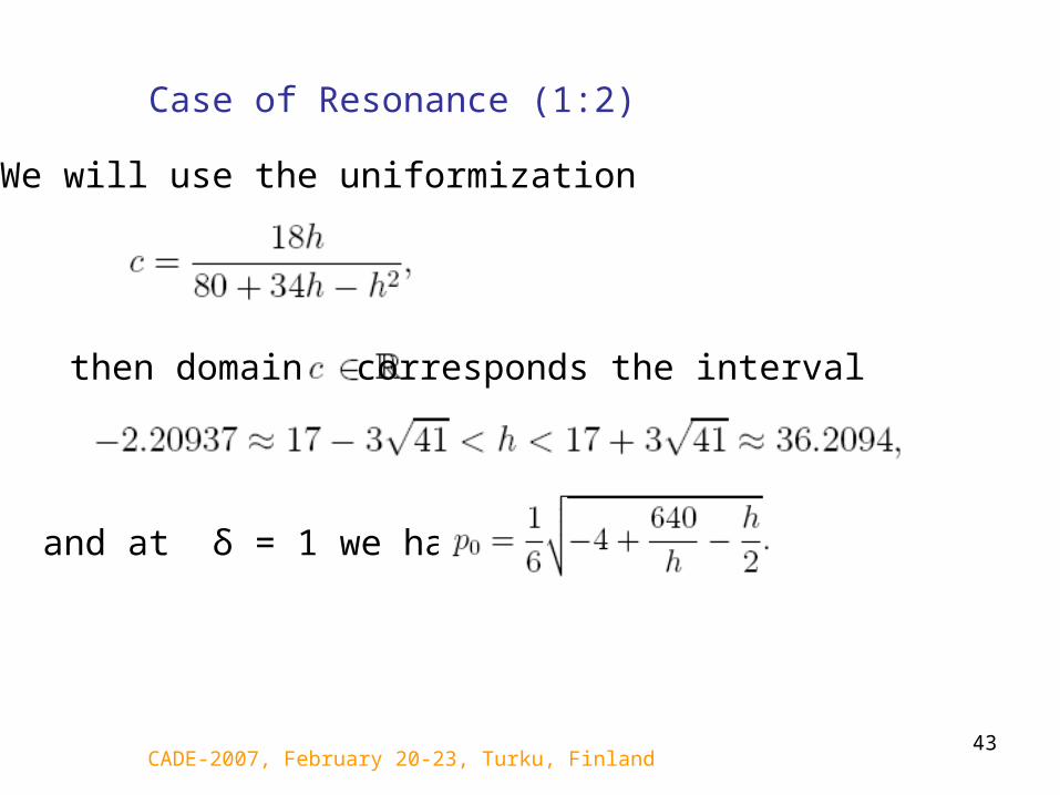
Case of Resonance (1:2)
We will use the uniformization
then domain corresponds the interval
and at δ = 1 we have
CADE-2007, February 20-23, Turku, Finland44
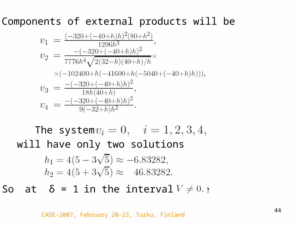
Components of external products will be
The system
will have only two solutions
So at δ = 1 in the interval above
CADE-2007, February 20-23, Turku, Finland45
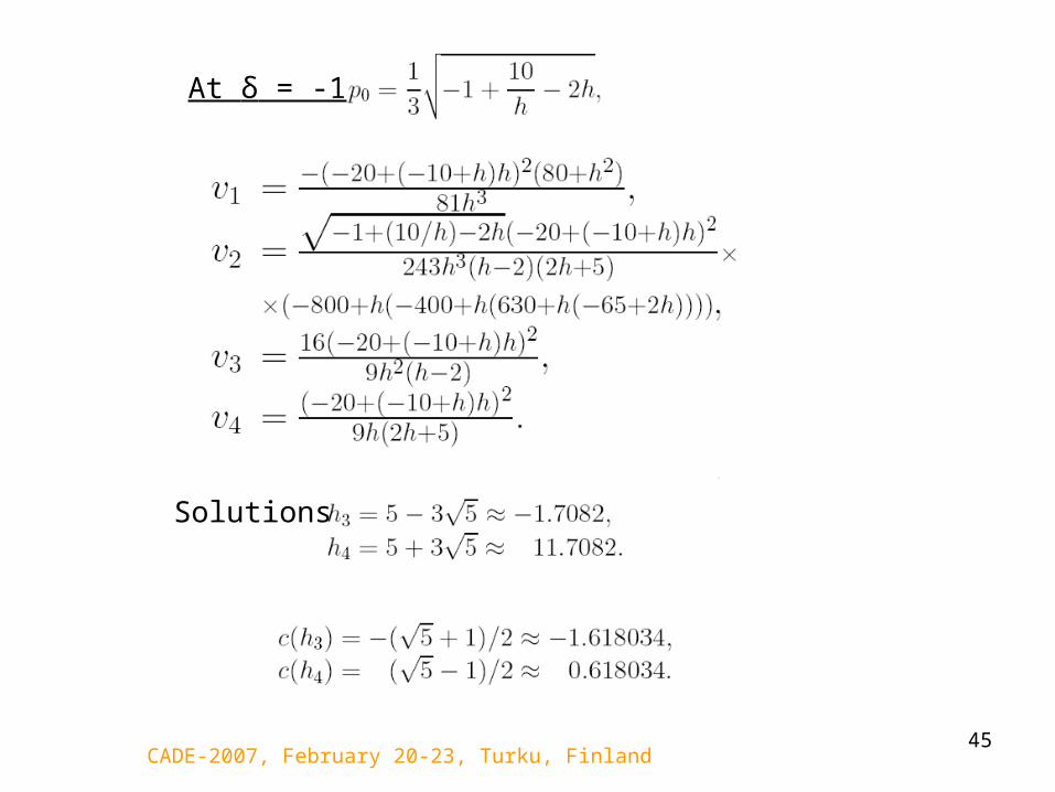
At δ = -1
Solutions

CADE-2007, February 20-23, Turku, Finland46
So only solution h4 lies in the mechanical semi-interval
But h4 is a special point with all zero eigenvalues and we can conclude that
With respect of the Main theorem of existence of an additional integral
1. Ξ ≠ 0 and V = 0,2. Ξ = 0 and rank(M) < 2,
we should look for points where Ξ = 0.
CADE-2007, February 20-23, Turku, Finland47
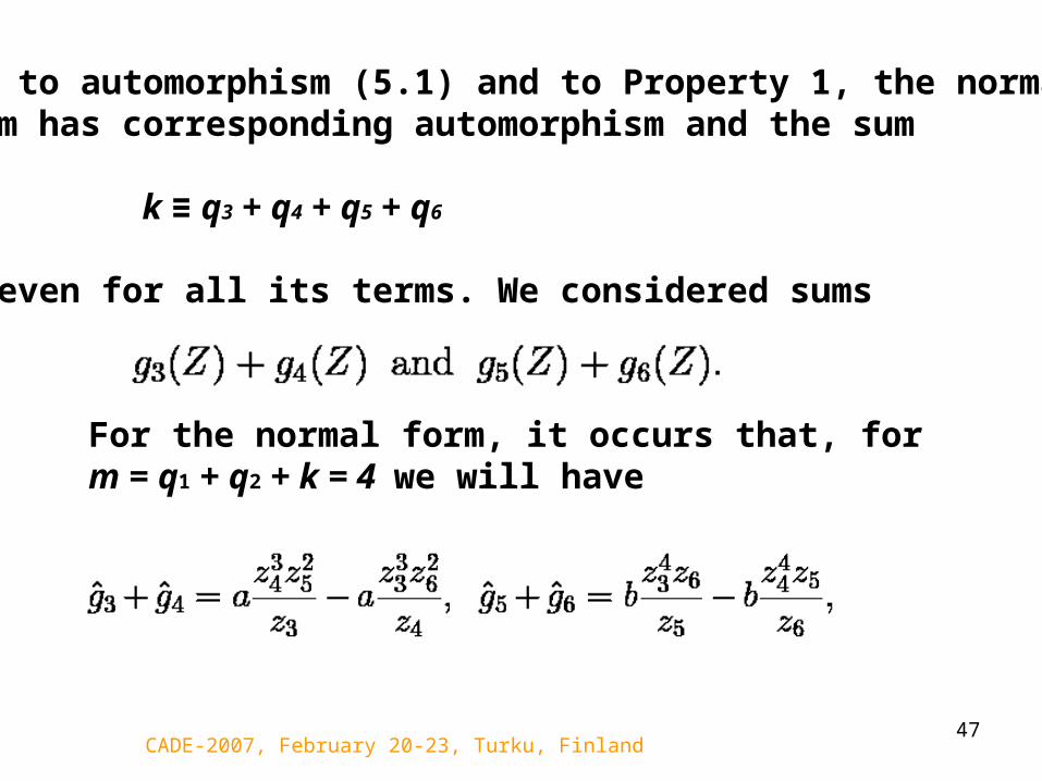
Due to automorphism (5.1) and to Property 1, the normal form has corresponding automorphism and the sum
k ≡ q3 + q4 + q5 + q6
is even for all its terms. We considered sums
For the normal form, it occurs that, for m = q1 + q2 + k = 4 we will have

CADE-2007, February 20-23, Turku, Finland48
and all lower terms cancel. Here, the quantities with a hat ĝk, k = 1, …, 6, denote the normal forms calculated up to order four.
It can be demonstrated that the vector Ξ has a components
,11
2
6
4
3^
zzzg
,22
2
6
4
3
2
^
zzzg
,3
a ,4
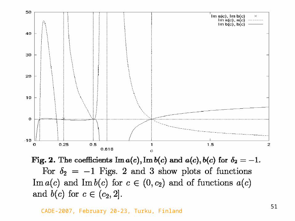
bSo we can calculate Ξ now. Coefficients a and b depend on δ2 and c. For δ2 = 1, both coefficients a and b are pure imaginary. For δ2 = –1, they are pure imaginary if c (0, c2) and are real if c (c2, 2].

CADE-2007, February 20-23, Turku, Finland50
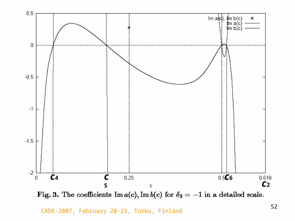
c3 c2
CADE-2007, February 20-23, Turku, Finland51
CADE-2007, February 20-23, Turku, Finland52
c4 c5 c6c2
CADE-2007, February 20-23, Turku, Finland54
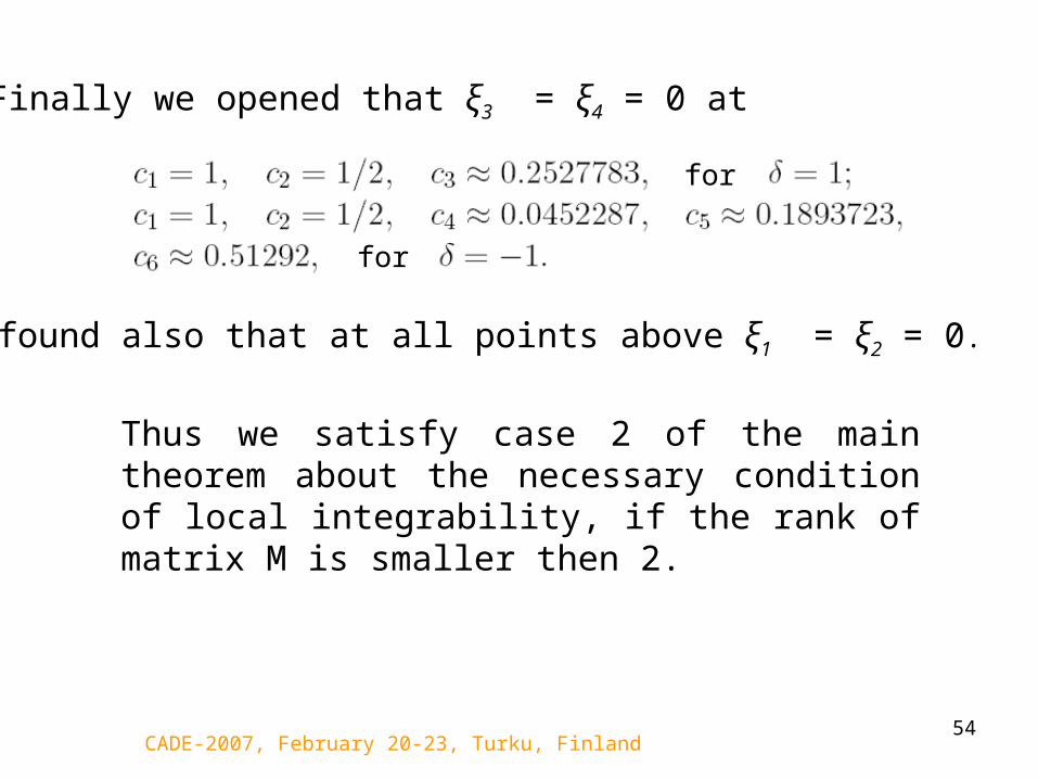
Finally we opened that ξ3 = ξ4 = 0 at
for
for
Thus we satisfy case 2 of the main theorem about the necessary condition of local integrability, if the rank of matrix M is smaller then 2.
We found also that at all points above ξ1 = ξ2 = 0.

CADE-2007, February 20-23, Turku, Finland55
We calculated the matrix M and its rank at the all points where Ξ = 0. Particularly at c = ½ the matrix M is
for
for
CADE-2007, February 20-23, Turku, Finland56
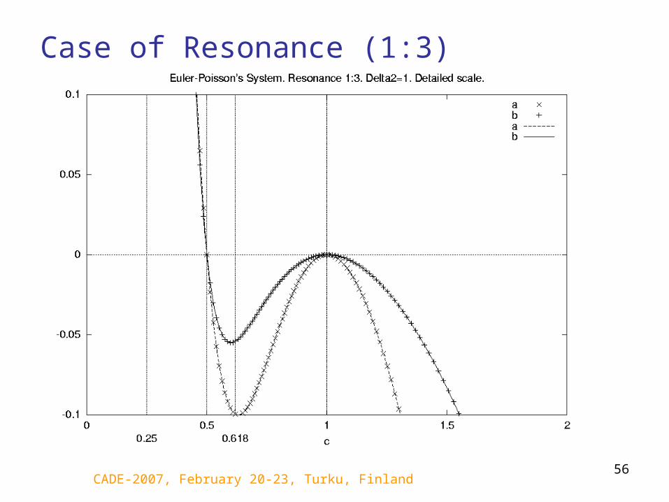
Case of Resonance (1:3)

CADE-2007, February 20-23, Turku, Finland57
c7=1/9

CADE-2007, February 20-23, Turku, Finland58
We calculated rank(M) at the points above and opened, thatit is equal to 2 in all cases except point c = ½, where this rankis equal 1 and point c = 1, where it has a zero value.
CADE-2007, February 20-23, Turku, Finland59
Conclusions
• The normalized system of Euler – Poisson has no additional formal integrals at the mechanical values of the parameter c in resonances (1:2) and (1:3), i.e., it is nonintegrable, except known cases c = ½ and c = 1.
• We have a new workable approach for searching additional formal integrals.
• We have a new method for a proof of nonintegrability in some domains.

CADE-2007, February 20-23, Turku, Finland60
References
Bruno, A.D.: Theory of normal forms of the Euler – Poisson equations. Preprint of the Keldysh Institute of Applied Mathematics of RAS No 100. Moscow (2005).
Lunkevich, V.A,, Sibirskii, K.S., Integrals of General Differential System at theCase of Center. Differential Equation, v. 18, No 5 (1982) 786–792, in Russian.

CADE-2007, February 20-23, Turku, Finland61
Absence of formal integral
Nonintegrability of shortened system
Nonintegrability of original system
Absence of local integral