Northfield’s 13th Annual Summer Seminar Friday, June 8th, 2007

Agenda Fat Tails, Tall Tales, Puppy Dog Tails

Dan diBartolomeo, Northfield Information Services

Improving Returns-Based Style Analysis Daniel Mostovoy, Northfield Information Services How Large is the Equity Premium Today? Samuel Thompson, Arrow Street Capital Implied Risk Acceptance Parameters (RAPs) in the Execution of Institutional Equity Trades

Thorsten Schmidt, CFA, Instinet

Alpha Scaling Revisited Anish Shah, Northfield Information Services

Distinguishing Between Being Unlucky and Unskillful Dan diBartolomeo, Northfield Information Services

Fat Tails, Tall Tales, Fat Tails, Tall Tales, Puppy Dog TailsPuppy Dog Tails

Dan diBartolomeoDan diBartolomeoAnnual Summer Seminar Annual Summer Seminar –– Newport, RINewport, RI

June 8, 2007June 8, 2007

Goals for this TalkGoals for this Talk

•• Survey and navigate the enormous literature in Survey and navigate the enormous literature in this areathis area

•• Review the debate on assumed distributions for Review the debate on assumed distributions for stock returnsstock returns

•• Consider the implications of the various possible Consider the implications of the various possible conclusions on asset pricing, portfolio conclusions on asset pricing, portfolio construction and risk managementconstruction and risk management

Return DistributionsReturn Distributions•• While traditional portfolio theory assumes that returns While traditional portfolio theory assumes that returns

for equity securities and market are normally distributed, for equity securities and market are normally distributed, there is a vast amount of empirical evidence that the there is a vast amount of empirical evidence that the frequency of large magnitude events frequency of large magnitude events seems much seems much greater than is predicted by the normal distribution with greater than is predicted by the normal distribution with observed sample variance parametersobserved sample variance parameters

•• Three broad schools of thought:Three broad schools of thought:–– Equity returns have stable distributions of infinite variance.Equity returns have stable distributions of infinite variance.–– Equity returns have specific, identifiable distributions that haEquity returns have specific, identifiable distributions that have ve

significant kurtosis (fat tails) relative to the normal distribusignificant kurtosis (fat tails) relative to the normal distribution tion (e.g. a gamma distribution)(e.g. a gamma distribution)

–– Distributions of equity returns are normal at each instant of Distributions of equity returns are normal at each instant of time, but look fat tailed due to time series fluctuations in thetime, but look fat tailed due to time series fluctuations in thevariancevariance

Stable Pareto DistributionsStable Pareto Distributions

•• Mandelbrot (1963) argues that extreme events are far Mandelbrot (1963) argues that extreme events are far too frequent in financial data series for the normal too frequent in financial data series for the normal distribution to hold. He argues for a stable distribution to hold. He argues for a stable ParetianParetianmodel, which has the uncomfortable property of infinite model, which has the uncomfortable property of infinite variancevariance

•• Mandelbrot (1969) provides a compromise, allowing for Mandelbrot (1969) provides a compromise, allowing for “locally Gaussian processes”“locally Gaussian processes”

•• FamaFama (1965) provides empirical tests of Mandelbrot’s (1965) provides empirical tests of Mandelbrot’s idea on daily US stock returns. Finds fat tails, but also idea on daily US stock returns. Finds fat tails, but also volatility clusteringvolatility clustering

•• Lau, Lau and Lau, Lau and WingenderWingender (1990) reject the stable (1990) reject the stable distribution hypothesisdistribution hypothesis

•• RachevRachev (2000, 2003) deeply explores the mathematics (2000, 2003) deeply explores the mathematics of stable distributionsof stable distributions

A Bit on Stable DistributionsA Bit on Stable Distributions

•• General stable distributions have four parametersGeneral stable distributions have four parameters–– Location (replaces mean)Location (replaces mean)–– Scale (replaces standard deviation)Scale (replaces standard deviation)–– SkewSkew–– Tail Fatness Tail Fatness

•• Some moments are infiniteSome moments are infinite•• Except for some special cases (e.g. normal) there are no Except for some special cases (e.g. normal) there are no

analytical expressions for the likelihood functionsanalytical expressions for the likelihood functions•• Estimation of the parameters is very fragile. Many, Estimation of the parameters is very fragile. Many,

many different combinations of the four parameters can many different combinations of the four parameters can fit data equally wellfit data equally well

•• These distributions do have time scaling (you should be These distributions do have time scaling (you should be able to scale from daily observations to monthly able to scale from daily observations to monthly observations, etc.)observations, etc.)

Specific Fat Tailed DistributionSpecific Fat Tailed Distribution

•• Gulko (1999) argues that an efficient market Gulko (1999) argues that an efficient market corresponds to a state where the informational entropy corresponds to a state where the informational entropy of the system is maximizedof the system is maximized

•• Finds the riskFinds the risk--neutral probabilities that maximize entropyneutral probabilities that maximize entropy•• The entropy maximizing risk neutral probabilities are The entropy maximizing risk neutral probabilities are

equivalent to returns having the Gamma distributionequivalent to returns having the Gamma distribution•• Gamma has fat tails but only two parameters and finite Gamma has fat tails but only two parameters and finite

momentsmoments•• Has finite lower bound which fits nicely with the lower Has finite lower bound which fits nicely with the lower

bound on returns (i.e. bound on returns (i.e. --100%)100%)•• Derives an option pricing model of which BlackDerives an option pricing model of which Black--ScholesScholes

is a special caseis a special case

Time Varying VolatilityTime Varying Volatility•• The alternative to stable fatThe alternative to stable fat--tailed distributions is that tailed distributions is that

returns are normally distributed at each moment in time, returns are normally distributed at each moment in time, but with time varying volatility, giving the illusion of fat but with time varying volatility, giving the illusion of fat tails when a long period is examinedtails when a long period is examined

•• Rosenberg (1974?)Rosenberg (1974?)–– Most kurtosis in financial time series can be explained by Most kurtosis in financial time series can be explained by

predictable predictable time series variation in the volatility of a normal time series variation in the volatility of a normal distributiondistribution

•• Engle and Engle and BollerslevBollerslev: ARCH/GARCH models: ARCH/GARCH models–– Models that presume that volatility events occur in clustersModels that presume that volatility events occur in clusters–– Huge literature. I stopped counting when I hit 250 papers in Huge literature. I stopped counting when I hit 250 papers in

referred journals as of 2003referred journals as of 2003•• LeBaronLeBaron (2006)(2006)

–– Extensive empirical analysis of stock returnsExtensive empirical analysis of stock returns–– Finds strong support for time varying volatility, but very weak Finds strong support for time varying volatility, but very weak

evidence of actual kurtosisevidence of actual kurtosis

The Remarkable Rosenberg PaperThe Remarkable Rosenberg Paper

•• Unpublished paper by Barr Rosenberg (1974?), under US Unpublished paper by Barr Rosenberg (1974?), under US National Science Foundation Grant 3306National Science Foundation Grant 3306

•• Builds detailed model of timeBuilds detailed model of time--varying volatility in which varying volatility in which long run kurtosis arises from two sourceslong run kurtosis arises from two sources–– The kurtosis of a population is an accumulation of the kurtosis The kurtosis of a population is an accumulation of the kurtosis

across each sample subacross each sample sub--periodperiod–– Time varying volatility and serial correlation can induce the Time varying volatility and serial correlation can induce the

appearance of kurtosis when the distribution at any one moment appearance of kurtosis when the distribution at any one moment in time is normalin time is normal

–– Predicts more kurtosis for high frequency dataPredicts more kurtosis for high frequency data•• An empirical test on 100 years of monthly US stock index An empirical test on 100 years of monthly US stock index

returns shows an Rreturns shows an R--squared of .86squared of .86•• Very reminiscent of subsequent ARCH/GARCH modelsVery reminiscent of subsequent ARCH/GARCH models

ARCH/GARCHARCH/GARCH

•• Engle (1982) for ARCH, Engle (1982) for ARCH, BollerslevBollerslev (1986) for GARCH(1986) for GARCH•• Conditional heteroscedasticity models are standard Conditional heteroscedasticity models are standard

operating procedure in most financial market operating procedure in most financial market applications with high frequency dataapplications with high frequency data

•• They assume that volatility occurs in clusters, hence They assume that volatility occurs in clusters, hence changes in volatility are predictablechanges in volatility are predictable

•• Andersen, Andersen, BollerslevBollerslev, , DieboldDiebold and and LabysLabys (2000)(2000)–– Exchange rate returns are GaussianExchange rate returns are Gaussian

•• Andersen, Andersen, BollerslevBollerslev, , DieboldDiebold and and EbensEbens (2001)(2001)–– The distribution of stock return variance is right skewed for The distribution of stock return variance is right skewed for

arithmetic returns, normal for log returnarithmetic returns, normal for log return–– Stock returns must be Gaussian because the distribution of Stock returns must be Gaussian because the distribution of

returns/volatility is unit normalreturns/volatility is unit normal

Recent Empirical ResearchRecent Empirical Research

•• LebaronLebaron, , SamantaSamanta and and CecchettiCecchetti (2006)(2006)•• Exhaustive MonteExhaustive Monte--Carlo bootstrap tests of various fat Carlo bootstrap tests of various fat

tailed distributions to daily Dow Jones Index data using tailed distributions to daily Dow Jones Index data using robust estimatorsrobust estimators

•• Propose a novel adjustment for time scaling volatilities to Propose a novel adjustment for time scaling volatilities to account for kurtosis, in order to use daily data to account for kurtosis, in order to use daily data to forecast monthly volatilityforecast monthly volatility

•• Conclusion: “No compelling evidence that 4Conclusion: “No compelling evidence that 4thth moments moments exist”exist”–– If variance is unstable, then its difficult to estimateIf variance is unstable, then its difficult to estimate–– High frequency data is less usefulHigh frequency data is less useful–– Use robust estimators of volatilityUse robust estimators of volatility–– Estimation error of expected returns dominates variance in Estimation error of expected returns dominates variance in

forming optimal portfoliosforming optimal portfolios

More Work on Fat TailsMore Work on Fat Tails

•• Japan Stock ReturnsJapan Stock Returns–– AggarwalAggarwal, , RaoRao and and HirakiHiraki (1989) (1989) –– Watanabe (2000)Watanabe (2000)

•• France Stock ReturnsFrance Stock Returns–– NavatteNavatte, , ChristopheChristophe Villa (2000)Villa (2000)

•• Option implied kurtosisOption implied kurtosis–– CorradoCorrado and Su (1996, 1997a, 1997b)and Su (1996, 1997a, 1997b)–– Brown and Robinson (2002)Brown and Robinson (2002)

•• Sides of the debateSides of the debate–– Lee and Wu (1985)Lee and Wu (1985)–– Tucker (1992)Tucker (1992)–– GhoseGhose and and KronerKroner (1995)(1995)–– MittnikMittnik, , PaolellaPaolella and and RachevRachev (2000)(2000)–– RockingerRockinger and and JondeauJondeau (2002)(2002)

The Time Scale IssueThe Time Scale Issue

•• Almost all empirical work shows that fat tails are more Almost all empirical work shows that fat tails are more prevalent with high frequency (i.e. daily rather than prevalent with high frequency (i.e. daily rather than monthly) return observationsmonthly) return observations

•• Lack of fat tails in low frequency data is problem for Lack of fat tails in low frequency data is problem for proponents of stable distributions, proponents of stable distributions, –– the tail properties should time scalethe tail properties should time scale–– maybe we just don’t have enough observations when we use maybe we just don’t have enough observations when we use

lower frequency data for apparent kurtosis to be statistically lower frequency data for apparent kurtosis to be statistically significantsignificant

•• Or the observed differences in higher moments could be Or the observed differences in higher moments could be a mathematical artifact of the way returns are being a mathematical artifact of the way returns are being calculatedcalculated–– Lau and Lau and WingenderWingender (1989) call this the “(1989) call this the “intervalingintervaling effect”effect”

The Curious Compromise of The Curious Compromise of FinanalyticaFinanalytica•• The basic concepts of stable fat tailed distributions and The basic concepts of stable fat tailed distributions and

timetime--varying volatility models are clearly mutually varying volatility models are clearly mutually exclusive as explanations for the observed empirical dataexclusive as explanations for the observed empirical data

•• From the From the FinanalyticaFinanalytica website:website:–– “uses proprietary generalized multivariate stable (“uses proprietary generalized multivariate stable (GMstableGMstable) )

distributions as the central foundation of its risk management distributions as the central foundation of its risk management and portfolio optimization solutions”and portfolio optimization solutions”

–– “Clustering of volatility effects are well known to anyone who “Clustering of volatility effects are well known to anyone who has traded securities during periods of changing market has traded securities during periods of changing market volatility. volatility. FinanalyticaFinanalytica uses advanced volatility clustering models uses advanced volatility clustering models such as stable GARCH…”such as stable GARCH…”

•• SvetlozarSvetlozar RachevRachev and Doug Martin are really smart guys and Doug Martin are really smart guys so I’m putting this down to pragmatism rather than so I’m putting this down to pragmatism rather than schizophreniaschizophrenia

Kurtosis versus SkewKurtosis versus Skew

•• So far we’ve talked largely about 4So far we’ve talked largely about 4thth momentsmoments•• We haven’t done much in terms of economic arguments We haven’t done much in terms of economic arguments

about why fat tails exist, and at least appear to be more about why fat tails exist, and at least appear to be more prevalent with higher frequency dataprevalent with higher frequency data

•• Many of the same arguments apply to skew (one fat Many of the same arguments apply to skew (one fat tail), tail), –– consistent prevalence of negative skew in financial data seriesconsistent prevalence of negative skew in financial data series

•• Harvey and Harvey and SiddiqueSiddique (1999) find that skew can be (1999) find that skew can be predicted using an autoregressive scheme similar to predicted using an autoregressive scheme similar to GARCHGARCH

CrossCross--Sectional DispersionSectional Dispersion

•• When we think about “fat tails” we are usually thinking When we think about “fat tails” we are usually thinking about time series observations of returnsabout time series observations of returns

•• For active managers, the crossFor active managers, the cross--section of returns may be section of returns may be even more important, as it defines the opportunity set even more important, as it defines the opportunity set

•• DeSilvaDeSilva, , SapraSapra and and ThorleyThorley (2001) (2001) –– if asset specific risk varies across stocks, the crossif asset specific risk varies across stocks, the cross--section section

should be expected to have a should be expected to have a unimodalunimodal, fat, fat--tailed distributiontailed distribution

•• AlmgrenAlmgren and and ChrissChriss (2004)(2004)–– provides a substitute for “alpha scaling” that sorts stocks by provides a substitute for “alpha scaling” that sorts stocks by

attractiveness criteria, then maps the sorted values into a fatattractiveness criteria, then maps the sorted values into a fat--tailed multivariate distribution using copula methodstailed multivariate distribution using copula methods

What’s the Problem What’s the Problem with Daily Returns Anyway?with Daily Returns Anyway?

•• Financial markets are driven by the arrival of information Financial markets are driven by the arrival of information in the form of “news” (truly unanticipated) and the form in the form of “news” (truly unanticipated) and the form of “announcements” that are anticipated with respect to of “announcements” that are anticipated with respect to time but not with respect to content. time but not with respect to content.

•• The time intervals it takes markets to absorb and adjust The time intervals it takes markets to absorb and adjust to new information ranges from minutes to days. to new information ranges from minutes to days. Generally much smaller than a month, but up to and Generally much smaller than a month, but up to and often larger than a day. That’s why US markets were often larger than a day. That’s why US markets were closed for a week at September 11closed for a week at September 11thth..

Investor Response to InformationInvestor Response to Information

•• Several papers have examined the relative market Several papers have examined the relative market response to response to ““newsnews”” and and ““announcementsannouncements””–– EderingtonEderington and Lee (1996)and Lee (1996)–– KwagKwag ShrievesShrieves and Wansley(2000)and Wansley(2000)–– Abraham and Taylor (1993) Abraham and Taylor (1993)

•• Jones, Lamont and Jones, Lamont and LumsdaineLumsdaine (1998) show a (1998) show a remarkable result for the US bond marketremarkable result for the US bond market–– Total returns for long bonds and Treasury bills are not differenTotal returns for long bonds and Treasury bills are not different t

if announcement days are removed from the data setif announcement days are removed from the data set•• Brown, Harlow and Brown, Harlow and TinicTinic (1988) provide a framework for (1988) provide a framework for

asymmetrical response to “good” and “bad” news asymmetrical response to “good” and “bad” news –– Good news increases projected cash flows, bad news decreasesGood news increases projected cash flows, bad news decreases–– All new information is a “surprise”, decreasing investor All new information is a “surprise”, decreasing investor

confidence and increasing discount ratesconfidence and increasing discount rates–– Upward price movements are muted, while downward Upward price movements are muted, while downward

movements are accentuatedmovements are accentuated

Implications for Asset PricingImplications for Asset Pricing•• If investors price skew and/or kurtosis, there are If investors price skew and/or kurtosis, there are

implications for asset pricingimplications for asset pricing•• Harvey (1989) finds relationship between asset prices Harvey (1989) finds relationship between asset prices

and time varying and time varying covariancescovariances•• Kraus and Kraus and LitzenbergerLitzenberger (1976) and Harvey and (1976) and Harvey and SiddiqueSiddique

(2000) find that investors are averse to negative skew(2000) find that investors are averse to negative skew–– diBartolomeo (2003) argues that the value/growth relationship diBartolomeo (2003) argues that the value/growth relationship

in equity returns can be modeled as option payoffs, implying in equity returns can be modeled as option payoffs, implying skew in distributionskew in distribution

–– If the value/growth relationship has skew and investors price If the value/growth relationship has skew and investors price skew, then an efficient market will show a value premiumskew, then an efficient market will show a value premium

•• DittmarDittmar (2002) find that non(2002) find that non--linear asset pricing models linear asset pricing models for stocks work if a kurtosis preference is includedfor stocks work if a kurtosis preference is included

•• BarroBarro (2005) finds that the large equity risk premium (2005) finds that the large equity risk premium observed in most markets is justified under a “rare observed in most markets is justified under a “rare disaster” scenariodisaster” scenario

Portfolio Construction and Risk Portfolio Construction and Risk ManagementManagement

•• Kritzman and Rich (1998) define risk management Kritzman and Rich (1998) define risk management function when nonfunction when non--survival is possiblesurvival is possible

•• SatchellSatchell (2004)(2004)–– Describes the Describes the thethe diversification of skew and kurtosisdiversification of skew and kurtosis–– Illustrates that plausible utility functions will favor Illustrates that plausible utility functions will favor

positive skew and dislike kurtosispositive skew and dislike kurtosis

•• Wilcox (2000) shows that the importance of higher Wilcox (2000) shows that the importance of higher moments is an increasing function of investor gearingmoments is an increasing function of investor gearing

Optimization with Higher MomentsOptimization with Higher Moments•• ChamberlinChamberlin, Cheung and Kwan(1990) derive portfolio , Cheung and Kwan(1990) derive portfolio

optimality for multioptimality for multi--factor models under stable factor models under stable paretianparetianassumptionsassumptions

•• Lai (1991) derives portfolio selection based on Lai (1991) derives portfolio selection based on skewnessskewness•• Davis (1995) derives optimal portfolios under the Davis (1995) derives optimal portfolios under the

Gamma distribution assumptionGamma distribution assumption•• HlawitsckaHlawitscka and Stern (1995) show the simulated and Stern (1995) show the simulated

performance of mean variance portfolios is nearly performance of mean variance portfolios is nearly indistinguishable from the utility maximizing portfolioindistinguishable from the utility maximizing portfolio

•• CremersCremers, Kritzman and Paige (2003), Kritzman and Paige (2003)–– Use extensive simulations to measure the loss of utility Use extensive simulations to measure the loss of utility

associated with ignoring higher moments in portfolio associated with ignoring higher moments in portfolio constructionconstruction

–– They find that the loss of utility is negligible except for the They find that the loss of utility is negligible except for the special cases of concentrated portfolios or “kinked” utility special cases of concentrated portfolios or “kinked” utility functions (i.e. when there is risk of nonfunctions (i.e. when there is risk of non--survival). survival).

ConclusionsConclusions•• The fat tailed nature of high frequency returns is well The fat tailed nature of high frequency returns is well

establishedestablished•• The nature of the process is usually described as being a The nature of the process is usually described as being a

fat tailed stable distribution or a normal distribution with fat tailed stable distribution or a normal distribution with time varying volatilitytime varying volatility

•• The process that creates fat tailed distributions probably The process that creates fat tailed distributions probably has to do with rate at which markets can absorb new has to do with rate at which markets can absorb new informationinformation

•• The existence of fat tails and skew has important The existence of fat tails and skew has important implications for asset pricingimplications for asset pricing

•• Fat tails probably have relatively lesser importance for Fat tails probably have relatively lesser importance for portfolio formation, unless there are special conditions portfolio formation, unless there are special conditions such as gearing that imply nonsuch as gearing that imply non--standard utility functionsstandard utility functions

ReferencesReferences

•• Mandelbrot, Benoit. "LongMandelbrot, Benoit. "Long--Run Linearity, Locally Gaussian Process, Run Linearity, Locally Gaussian Process, HH--Spectra And Infinite Variances," International Economic Review, Spectra And Infinite Variances," International Economic Review, 1969, v10(1), 821969, v10(1), 82--111.111.

•• Mandelbrot, Benoit. "The Variation Of Certain Speculative PricesMandelbrot, Benoit. "The Variation Of Certain Speculative Prices," ," Journal of Business, 1963, v36(4), 394Journal of Business, 1963, v36(4), 394--419.419.

•• FamaFama, Eugene F. "The Behavior Of Stock Market Prices," Journal of , Eugene F. "The Behavior Of Stock Market Prices," Journal of Business, 1965, v38(1), 34Business, 1965, v38(1), 34--105.105.

•• Lau, Amy Lau, Amy HingHing--Ling, HonLing, Hon--ShiangShiang Lau And John R. Lau And John R. WingenderWingender. "The . "The Distribution Of Stock Returns: New Evidence Against The Stable Distribution Of Stock Returns: New Evidence Against The Stable Model," Journal of Business and Economic Statistics, 1990, v8(2)Model," Journal of Business and Economic Statistics, 1990, v8(2), , 217217--224.224.

•• RachevRachev, S.T. and S. , S.T. and S. MittnikMittnik (2000). Stable (2000). Stable ParetianParetian Models in Models in Finance, Wiley.Finance, Wiley.

ReferencesReferences•• RachevRachev, S.T. (editor) Handbook of Heavy Tailed Distributions in , S.T. (editor) Handbook of Heavy Tailed Distributions in

Finance. Elsevier.Finance. Elsevier.•• Gulko, L. "The Entropy Theory Of Stock Option Pricing," Gulko, L. "The Entropy Theory Of Stock Option Pricing,"

International Journal of Theoretical and Applied Finance, 1999, International Journal of Theoretical and Applied Finance, 1999, v2(3,Jul), 331v2(3,Jul), 331--356.356.

•• Rosenberg, Barr. “The Behavior of Random Variables with Rosenberg, Barr. “The Behavior of Random Variables with NonstationaryNonstationary Variance and the Distribution of Security Prices”, UC Variance and the Distribution of Security Prices”, UC Berkeley Working Paper, NSF 3306, 1974. Berkeley Working Paper, NSF 3306, 1974.

•• LebaronLebaron, Blake. , Blake. RitirupaRitirupa SamantaSamanta, and Stephen , and Stephen CecchettiCecchetti. “Fat Tails . “Fat Tails and 4and 4thth Moments: Practical Problems of Variance Estimation”, Moments: Practical Problems of Variance Estimation”, Brandeis University Working Paper, 2006. Brandeis University Working Paper, 2006.

•• Engle, Robert F. "Autoregressive Conditional Heteroscedasticity Engle, Robert F. "Autoregressive Conditional Heteroscedasticity With With Estimates Of The Variance Of United Kingdom Inflations," Estimates Of The Variance Of United Kingdom Inflations," EconometricaEconometrica, 1982, v50(4), 987, 1982, v50(4), 987--1008.1008.

•• BollerslevBollerslev, Tim. "Generalized Autoregressive Conditional , Tim. "Generalized Autoregressive Conditional HeteroskedasticityHeteroskedasticity," Journal of Econometrics, 1986, v31(3), 307," Journal of Econometrics, 1986, v31(3), 307--328.328.

referencesreferences

•• Andersen, Andersen, TorbenTorben G., Tim G., Tim BollerslevBollerslev, Francis X. , Francis X. DieboldDiebold and and HeikoHeikoEbensEbens. "The Distribution Of Realized Stock Return Volatility," Journa. "The Distribution Of Realized Stock Return Volatility," Journal l of Financial Economics, 2001, v61(1,Jul), 43of Financial Economics, 2001, v61(1,Jul), 43--76.76.

•• Andersen, Andersen, TorbenTorben G., Tim G., Tim BollerslevBollerslev, Francis X. , Francis X. DieboldDiebold and Paul and Paul LabysLabys. "Exchange Rate Returns Standardized By Realized Volatility . "Exchange Rate Returns Standardized By Realized Volatility Are (Nearly) Gaussian," Managerial Finance Journal, 2000, Are (Nearly) Gaussian," Managerial Finance Journal, 2000, v4(3/4,Sep/Dec), 159v4(3/4,Sep/Dec), 159--179.179.

•• AggarwalAggarwal, , RajRaj, , RameshRamesh P. P. RaoRao and and TakatoTakato HirakiHiraki. ". "SkewnessSkewness And And Kurtosis In Japanese Equity Returns: Empirical Evidence," JournaKurtosis In Japanese Equity Returns: Empirical Evidence," Journal of l of Financial Research, 1989, v12(3), 253Financial Research, 1989, v12(3), 253--260.260.

•• Watanabe, Toshiaki. "Excess Kurtosis Of Conditional DistributionWatanabe, Toshiaki. "Excess Kurtosis Of Conditional Distribution For For Daily Stock Returns: The Case Of Japan," Applied Economics Daily Stock Returns: The Case Of Japan," Applied Economics Letters, 2000, v7(6,Jun), 353Letters, 2000, v7(6,Jun), 353--355.355.

•• NavatteNavatte, Patrick and , Patrick and ChristopheChristophe Villa. "The Information Content Of Villa. "The Information Content Of Implied Volatility, Implied Volatility, SkewnessSkewness And Kurtosis: Empirical Evidence From And Kurtosis: Empirical Evidence From LongLong--Term CAC 40 Options," European Financial Management, Term CAC 40 Options," European Financial Management, 2000, v6(1,Mar), 412000, v6(1,Mar), 41--56.56.

ReferencesReferences•• CorradoCorrado, C. J. and Tie Su. "Implied Volatility Skews And Stock , C. J. and Tie Su. "Implied Volatility Skews And Stock

Return Return SkewnessSkewness And Kurtosis Implied By Stock Option Prices," And Kurtosis Implied By Stock Option Prices," European Journal of Finance, 1997, v3(1,Mar), 73European Journal of Finance, 1997, v3(1,Mar), 73--85.85.

•• CorradoCorrado, Charles J. and Tie Su. "Implied Volatility Skews And Stock , Charles J. and Tie Su. "Implied Volatility Skews And Stock Index Index SkewnessSkewness And Kurtosis Implied By S&P 500 Index Option And Kurtosis Implied By S&P 500 Index Option Prices," Journal of Derivatives, 1997, v4(4,Summer), 8Prices," Journal of Derivatives, 1997, v4(4,Summer), 8--19.19.

•• CorradoCorrado, Charles J. and Tie Su. ", Charles J. and Tie Su. "SkewnessSkewness And Kurtosis Of S&P 500 And Kurtosis Of S&P 500 Index Returns Implied By Option Prices," Journal of Financial Index Returns Implied By Option Prices," Journal of Financial Research, 1996, v19(2,Summer), 175Research, 1996, v19(2,Summer), 175--192.192.

•• Brown, Christine A. and David M. Robinson. "Brown, Christine A. and David M. Robinson. "SkewnessSkewness And Kurtosis And Kurtosis Implied By Option Prices: A Correction," Journal of Financial Implied By Option Prices: A Correction," Journal of Financial Research, 2002, v25(2,Summer), 279Research, 2002, v25(2,Summer), 279--282.282.

•• Lee, Cheng F. and Lee, Cheng F. and ChunchiChunchi Wu. "The Impacts Of Kurtosis On Risk Wu. "The Impacts Of Kurtosis On Risk StationarityStationarity: Some Empirical Evidence," Financial Review, 1985, : Some Empirical Evidence," Financial Review, 1985, v20(4), 263v20(4), 263--269.269.

•• Tucker, Alan L. "A Reexamination Of FiniteTucker, Alan L. "A Reexamination Of Finite-- And And InfinteInfinte--Variance Variance Distributions As Models Of Daily Stock Returns," Journal of BusiDistributions As Models Of Daily Stock Returns," Journal of Business ness and Economic Statistics, 1992, v10(1), 83and Economic Statistics, 1992, v10(1), 83--82.82.

ReferencesReferences

•• GhoseGhose, , DevajyotiDevajyoti and Kenneth F. and Kenneth F. KronerKroner. "Their Relationship . "Their Relationship Between GARCH And Symmetric Stable Processes: Finding The Between GARCH And Symmetric Stable Processes: Finding The Source Of Fat Tails In Financial Data," Journal of Empirical FinSource Of Fat Tails In Financial Data," Journal of Empirical Finance, ance, 1995, v2(3,Sep), 2251995, v2(3,Sep), 225--251.251.

•• MittnikMittnik, Stefan, Marc S. , Stefan, Marc S. PaolellaPaolella and and SvetlozarSvetlozar T. T. RachevRachev. . "Diagnosing And Treating The Fat Tails In Financial Returns Data"Diagnosing And Treating The Fat Tails In Financial Returns Data," ," Journal of Empirical Finance, 2000, v7(3Journal of Empirical Finance, 2000, v7(3--4,Nov), 3894,Nov), 389--416.416.

•• RockingerRockinger, Michael and Eric , Michael and Eric JondeauJondeau. "Entropy Densities With An . "Entropy Densities With An Application To Autoregressive Conditional Application To Autoregressive Conditional SkewnessSkewness And Kurtosis," And Kurtosis," Journal of Econometrics, 2002, v106(1,Jan), 119Journal of Econometrics, 2002, v106(1,Jan), 119--142.142.

•• Lau, HonLau, Hon--ShiangShiang and John R. and John R. WingenderWingender. "The Analytics Of The . "The Analytics Of The IntervalingIntervaling Effect On Effect On SkewnessSkewness And Kurtosis Of Stock Returns," And Kurtosis Of Stock Returns," Financial Review, 1989, v24(2), 215Financial Review, 1989, v24(2), 215--234.234.

•• Harvey, Campbell R. and Harvey, Campbell R. and AkhtarAkhtar SiddiqueSiddique. "Autoregressive . "Autoregressive Conditional Conditional SkewnessSkewness," Journal of Financial and Quantitative ," Journal of Financial and Quantitative Analysis, 1999, v34(4,Dec), 465Analysis, 1999, v34(4,Dec), 465--477.477.

ReferencesReferences

•• De Silva, De Silva, HarindraHarindra, Steven , Steven SapraSapra and Steven and Steven ThorleyThorley. "Return . "Return Dispersion And Active Management," Financial Analyst Journal, Dispersion And Active Management," Financial Analyst Journal, 2001, v57(5,Sep/Oct), 292001, v57(5,Sep/Oct), 29--42.42.

•• AlmgrenAlmgren, Robert and Neil , Robert and Neil ChrissChriss. “Portfolio Optimization without . “Portfolio Optimization without Forecasts”, Forecasts”, UniveristyUniveristy of Toronto Working Paper, 2004. of Toronto Working Paper, 2004.

•• EderingtonEderington and Lee, and Lee, ““Creation and Resolution of Market Creation and Resolution of Market Uncertainty: The Importance of Information Releases, Journal of Uncertainty: The Importance of Information Releases, Journal of Financial and Quantitative Analysis, 1996Financial and Quantitative Analysis, 1996

•• KwagKwag, , ShrievesShrieves and and WansleyWansley, , ““Partially Anticipated Events: An Partially Anticipated Events: An Application to Dividend AnnouncementsApplication to Dividend Announcements””, University of Tennessee , University of Tennessee Working Paper, March 2000Working Paper, March 2000

•• Abraham and Taylor, Abraham and Taylor, ““Pricing Currency Options with Scheduled and Pricing Currency Options with Scheduled and Unscheduled Announcement Effects on VolatilityUnscheduled Announcement Effects on Volatility””, Managerial and , Managerial and Decision Science 1993Decision Science 1993

•• Jones, Charles M., Owen Lamont and Robin L. Jones, Charles M., Owen Lamont and Robin L. LumsdaineLumsdaine. . "Macroeconomic News And Bond Market Volatility," Journal of "Macroeconomic News And Bond Market Volatility," Journal of Financial Economics, 1998, v47(3,Mar), 315Financial Economics, 1998, v47(3,Mar), 315--337.337.

ReferencesReferences•• Brown, Keith C., W. V. Harlow and Brown, Keith C., W. V. Harlow and SehaSeha M. M. TinicTinic. "Risk Aversion, . "Risk Aversion,

Uncertain Information, And Market Efficiency," Journal of FinancUncertain Information, And Market Efficiency," Journal of Financial ial Economics, 1988, v22(2), 355Economics, 1988, v22(2), 355--386.386.

•• Harvey, Campbell R. "TimeHarvey, Campbell R. "Time--Varying Conditional Varying Conditional CovariancesCovariances In Tests In Tests Of Asset Pricing Models," Journal of Financial Economics, 1989, Of Asset Pricing Models," Journal of Financial Economics, 1989, v24(2), 289v24(2), 289--318.318.

•• Kraus, Alan and Robert H. Kraus, Alan and Robert H. LitzenbergerLitzenberger. ". "SkewnessSkewness Preference And Preference And The Valuation Of Risk Assets," Journal of Finance, 1976, v31(4),The Valuation Of Risk Assets," Journal of Finance, 1976, v31(4),10851085--1100.1100.

•• Harvey, Campbell R. and Harvey, Campbell R. and AkhtarAkhtar SiddiqueSiddique. "Conditional . "Conditional SkewnessSkewness In In Asset Pricing Tests," Journal of Finance, 2000, v55(3,Jun), 1263Asset Pricing Tests," Journal of Finance, 2000, v55(3,Jun), 1263--1295.1295.

•• DittmarDittmar, Robert F. "Nonlinear Pricing Kernels, Kurtosis Preference, , Robert F. "Nonlinear Pricing Kernels, Kurtosis Preference, And Evidence From The Cross Section Of Equity Returns," Journal And Evidence From The Cross Section Of Equity Returns," Journal of of Finance, 2002, v57(1,Feb), 369Finance, 2002, v57(1,Feb), 369--403.403.

•• BarroBarro, Robert. “Asset Markets in the Twentieth Century”, , Robert. “Asset Markets in the Twentieth Century”, Harvard/NBER Working Paper, 2005. Harvard/NBER Working Paper, 2005.

•• Kritzman, Mark and Don Rich. "Risk Containment For Investors WitKritzman, Mark and Don Rich. "Risk Containment For Investors With h Multivariate Utility Functions," Journal of Derivatives, 1998, Multivariate Utility Functions," Journal of Derivatives, 1998, v5(3,Spring), 28v5(3,Spring), 28--44.44.

ReferencesReferences•• SatchellSatchell, Stephen. “The Anatomy of Portfolio , Stephen. “The Anatomy of Portfolio SkewnessSkewness and and

Kurtosis”, Trinity College Cambridge Working Paper, 2004.Kurtosis”, Trinity College Cambridge Working Paper, 2004.•• Wilcox, Jarrod W. "Better Risk Management," Journal of PortfolioWilcox, Jarrod W. "Better Risk Management," Journal of Portfolio

Management, 2000, v26(4,Summer), 53Management, 2000, v26(4,Summer), 53--64.64.•• Chamberlain, Trevor W., C. Sherman Cheung and Clarence C. Y. Chamberlain, Trevor W., C. Sherman Cheung and Clarence C. Y.

Kwan. "Optimal Portfolio Selection Using The General MultiKwan. "Optimal Portfolio Selection Using The General Multi--Index Index Model: A Stable Model: A Stable ParetianParetian Framework," Decision Sciences, 1990, Framework," Decision Sciences, 1990, v21(3), 563v21(3), 563--571.571.

•• Lai, Lai, TsongTsong--YueYue. "Portfolio Selection With . "Portfolio Selection With SkewnessSkewness: A Multiple: A Multiple--Objective Approach," Review of Quantitative Finance and Objective Approach," Review of Quantitative Finance and Accounting, 1991, v1(3), 293Accounting, 1991, v1(3), 293--306.306.

•• Davis, Ronald E. "Davis, Ronald E. "BacktestBacktest Results For A Portfolio Optimization Results For A Portfolio Optimization Model Using A Certainty Equivalent Criterion For Gamma DistributModel Using A Certainty Equivalent Criterion For Gamma Distributed ed Returns," Advances in Mathematical Programming and Finance, Returns," Advances in Mathematical Programming and Finance, 1995, v4(1), 771995, v4(1), 77--101.101.

•• CremersCremers, Jan, Mark Kritzman and , Jan, Mark Kritzman and SebastienSebastien Page 2003 “Portfolio Page 2003 “Portfolio Formation with Higher Moments and Plausible Utility”, Revere StrFormation with Higher Moments and Plausible Utility”, Revere Street eet Working Paper Series 272Working Paper Series 272--12, November. 12, November.

Improving Returns-Based Style Analysis

Daniel MostovoyNorthfield Newport Seminar

June 2007

2

Main Points For Today• Over the past 15 years, Returns-Based Style

Analysis become a very widely used analytical method

• We’re going to review RBSA and discuss useful several improvements to the basic technique– Confidence Intervals– Testing for Regime Change– Kalman Filter / Exponential Weighting– Adjusting for Heteroscedasticity

• Recently, RBSA has gained a new usage in connection with hedge fund replication strategies

3

Basic RBSA• First introduced as “Effective Asset Mix Analysis” by

Sharpe (1988, 1992). Given a time series of returns of a fund, we try to find the mix of market indices that most closely fits the fund returns

Rt = Σ j = 1 to n WjRjt + εt

Rt is the return on the fund during period tWj is the weight of index jRjt is the return on index j during period tN is the number of indicesεt is the residual for period t

Sum of Wj = 1, 0 < Wj < 1

Basically an OLS multiple regression with constrained coefficients

4

Refinement #1Confidence Intervals

• Like any other estimate we need to know if our style weights results are meaningful

• A style weight estimate of “10% small cap value” isn’t very useful if its really “10% +/- 50%”

• We can only analyze a fund to the extent that the spanning indices are not linear combinations of each other

• Correlation between the spanning indices can frequently cause very large confidence intervals on style weights, as the constraints on the coefficients mask multicolinearity that would be observable in an OLS regression

5

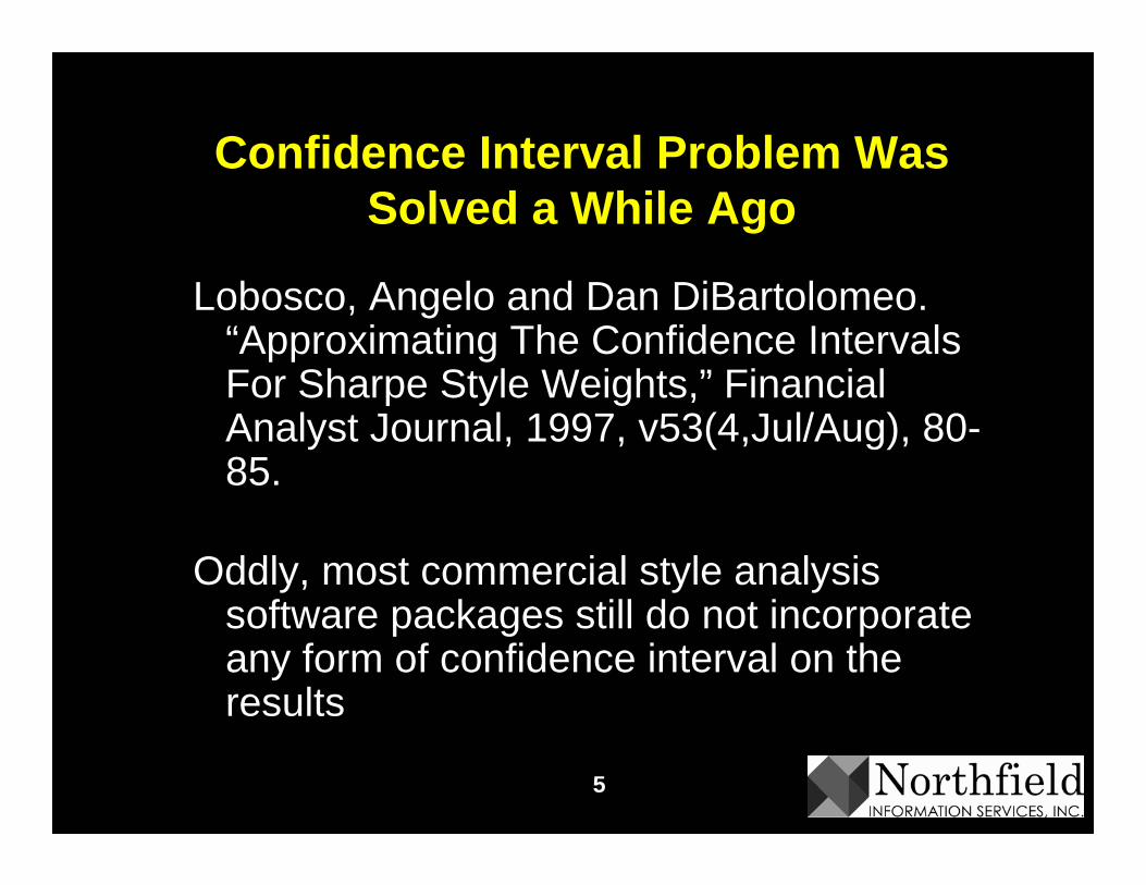
Confidence Interval Problem Was Solved a While Ago

Lobosco, Angelo and Dan DiBartolomeo. “Approximating The Confidence Intervals For Sharpe Style Weights,” Financial Analyst Journal, 1997, v53(4,Jul/Aug), 80-85.

Oddly, most commercial style analysis software packages still do not incorporate any form of confidence interval on the results

6

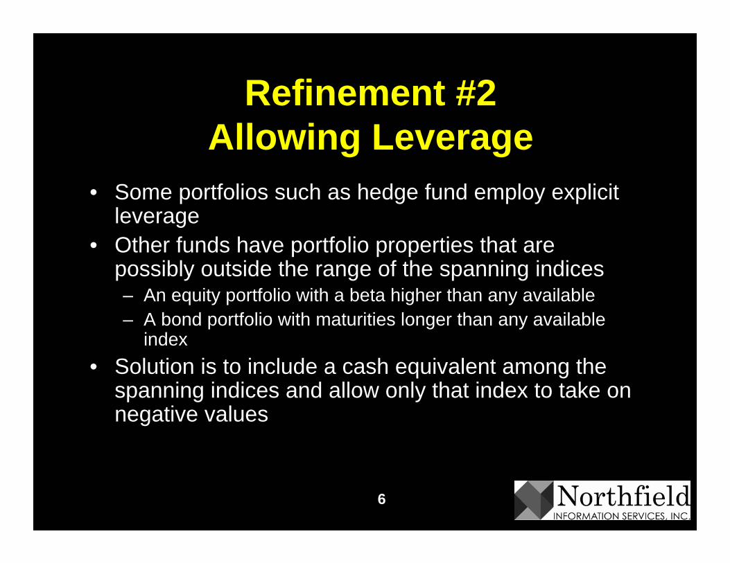
Refinement #2 Allowing Leverage

• Some portfolios such as hedge fund employ explicit leverage

• Other funds have portfolio properties that are possibly outside the range of the spanning indices– An equity portfolio with a beta higher than any available – A bond portfolio with maturities longer than any available

index • Solution is to include a cash equivalent among the

spanning indices and allow only that index to take on negative values

7

Refinement #3Testing for Regime Changes

• Do we want to look at fund results over the last 3 years, 5 years, 32 months, etc. ?

• CUSUM is an optimum statistic to determine the change in the mean of a process– Was adapted for the purposes of monitoring external asset

managers by the IBM pension fund• Use CUSUM based methods to determine the optimal "look-

back" period for the style analysis – Mathematically: What is the “look back” date such that the

cumulative active return between then and now is least likely tohave come about by random chance?

• Forthcoming paper by Bolster, diBartolomeo and Warrick summarized in our February 2005 newsletter– http://www.northinfo.com/documents/192.pdf

8

Refinement #4Capturing Recent Influences

• Traditional style weights represent the fund average behavior over a time sample– What we should be worried about is a fund that has changed

style recently, rendering “average” past information useless• One Approach

– Plot the absolute value of the residual against time during the sample

– If the slope is positive, the fit is getting worse as we come forward in time. Exponentially weight observations until the slope is not statistically significantly positive

• Another way is to use Kalman filtering – Swinkels, Laurens and Peter Van Der Sluis, “Returns based

Style Analysis with Time Varying Exposures”, ABP Working Paper, 2001

– Kalman filtering requires use of Markov Chain Monte-Carlo analysis if style weights are constrained to be positive

9

Refinement #5Asking the Right Question

• An easy experiment– Nine year sample period from 1998 through 2006– Make up a monthly return stream for a hypothetical fund

whose returns are equal to the S&P 500 for 1/3 of the 9 years, equal to the FTSE Europe for 1/3 of the 9 years, and equal to the Merrill Lynch Global High Yield for 1/3 of the 9 years

– First intuition suggests style weights should be 1/3 S&P 500, 1/3 FTSE Europe and 1/3 MLGHY

• Generally WRONG. It depends on the order of events

10

A Curious Result

46.54053.460.718.77.29SPMLFT

1.5634.3964.040.87-0.745.79SPFTML

38.5637.5923.850.71-2.166.89MLSPFT

36.4458.015.540.75-5.336.61MLFTSP

16.6543.4439.90.85-3.435.49FTSPML

59.6928.6611.650.672.876.63FTMLSP

MLGHYFTSE S&PR^2αSE

11

What’s Going On• The results are order dependent

– The style analysis process, like a regression is minimizing the sum of squared residuals

– The volatility of markets is different across the three sub-periods, and the more volatile periods are counted more heavily

– Not only do the weights vary across the different orders but goodness of fit changed a lot too

• Variation in alpha estimates ranged from -5.33 to + 8.7– This huge difference in alpha arises from the “accidental”

market timing arising from the ordering• Averaged across all six possible orders we get our

expected result of 1/3, 1/3, 1/3 for weights

12

Refinement #5Asking the Right Question

• The more volatile periods do count for more in the returns experienced by investors– If we want to know what market returns influenced the returns of

the fund, this is the right answer– This corresponds to Sharpe’s original concept of “Effective Asset

Mix”• But if we want to know whether a manager’s style was

consistent with a prescribed strategy, we have to filter out theeffects of heteroscedasticity within the sample period– For each time period calculate the “spanning dispersion”, the

average absolute difference in return between all possible pairswithin the spanning indices

– Weight the observations inversely with the square root of the dispersion

13

Refinement #6Volatility Based Spanning Indices

• Many hedge fund strategies are predicted on the level of market volatility, rather than expected returns– Purported uncorrelated with the direction of markets (e.g.

writing option spreads)• Fung and Hsieh (2002) suggest spanning indices that

are volatility related– Relative returns between mortgage backed securities and

coupon bonds are sensitive to interest rate volatility– Bondarenko (2004) constructs a index where the return is

based on the difference between implied and realized OEX volatility

– diBartolomeo (2006) reviews literature on dispersion of security returns within asset classes, http://www.northinfo.com/documents/234.pdf

14

Using RBSA to Proxy Hedge Fund Holdings

• A common problem in the hedge fund industry is the need to analyze a hedge fund where the holdings of the fund are not disclosed– Create a proxy portfolio for risk management and asset allocation

purposes– Hold the proxy portfolio as a “synthetic” version of the fund

• We will illustrate a procedure for estimating proxy holdings for a fund where the true underlying holdings are unknown.– Using a combination of returns based style analysis and portfolio

optimization• Our proxy portfolio is not meant to be a guess at the true

underlying portfolio, but rather an efficient estimate of:– The typical style bets of the fund– The degree of portfolio concentration– The balance between asset specific and factor risks.

15

Selecting the Spanning Indices• For each fund we need to select the right set of spanning

indices• Over a universe of funds, some indices will be significant lots of

funds, some indices will be significant to only a few funds• Use what we know about the fund strategy to manually select a

set of “likely suspects”• Start with a large list of indices. Iteratively run the analysis

dropping out the least statistically significant. – Easy to get fooled because T stats on indices improve as we drop

correlated but less significant indices• Start with a short list of indices representing major asset classes

– Run analysis, drop insignificant asset classes. Replace remaining indices with sub-indices. Rerun analysis and again drop out insignificant indices

16

RBSA Analysis Output

By running the style analysis, we get three pieces of information:– Observed volatility of the subject hedge fund during

chosen sample period– The "style" exposures of the subject fund (growth,

value, short volatility, etc.) expressed as percentages of the different indices that best mimic the fund’s return behavior over time.

– The relative proportion of risk coming from style factors and from fund specific risk.

17

Now Let Us Start to Form Holdings

• Take the constituents of our spanning indices and form a portfolio of these constituents weighted by results of the styleanalysis.

• If our style analysis said the fund behaved like 50% the S&P 500 and 50% EAFE

• We would form a portfolio that was 50% the weighted constituents of the S&P 500 and 50% EAFE.– At this point, we should have a portfolio that has the right "style"

exposures to match our fund • However, these two indices together have about 1600 stocks.• The resulting portfolio would be far too diversified to represent a

typical hedge fund. – It is likely to have far lower risk than a real hedge fund portfolio.

18

Let’s Refine the Proxy Holdings

Now we’ll consider portfolio volatility• Load the proxy portfolio into the Optimizer as both the

benchmark and the starting portfolio.– In our example, our version starting portfolio/benchmark would

have 1600 stocks.• We must reduce the number of positions such that the overall

risk of the portfolio approximates the observed risk of the subject fund.– We can do this by running an optimization while using the

"Maximum number of Assets" parameter.• With a little trial and error, we can find the portfolio that matches

the benchmark (and the subject fund) in style.– We reduce the diversification to the point where the expected

volatility of the proxy portfolio matches the observed volatility of the subject hedge fund.

19

Check the Balance Between Factor and Asset Specific Risks

• We now load the refined (reduced number of positions) proxy portfolio into the Optimizer as the portfolio with a cash benchmark.

• By running a risk report, we can determine how much of:– the expected risk of the refined proxy portfolio

arises from factor bets– Arises from asset specific risk.– If this is a reasonable match to the subject fund

(from the style analysis) we're done.

20

Changing the Balance Between Factor and Asset Specific Risks

• If we find we don’t have the appropriate balance between factor and asset specific risks– Repeat the process of “refining” the proxy portfolio– In addition to defining the Max Assets parameter, we can

change the Optimizer’s degree of risk tolerance for factor and asset specific risk

– Again with a little trial and error, we can find risk acceptanceparameter values that bring the relative proportions of factor risk and asset specific risk into line with our analysis of the subject fund

• We now have our proxy portfolio to hold or use as a composite asset in other analyses

21

Conclusions

• The effectiveness of Returns Based Style Analysis can be enhanced in a number of important ways

• These enhancements are particularly important in analyzing funds where substantial shifts in strategy may be expected over time

22

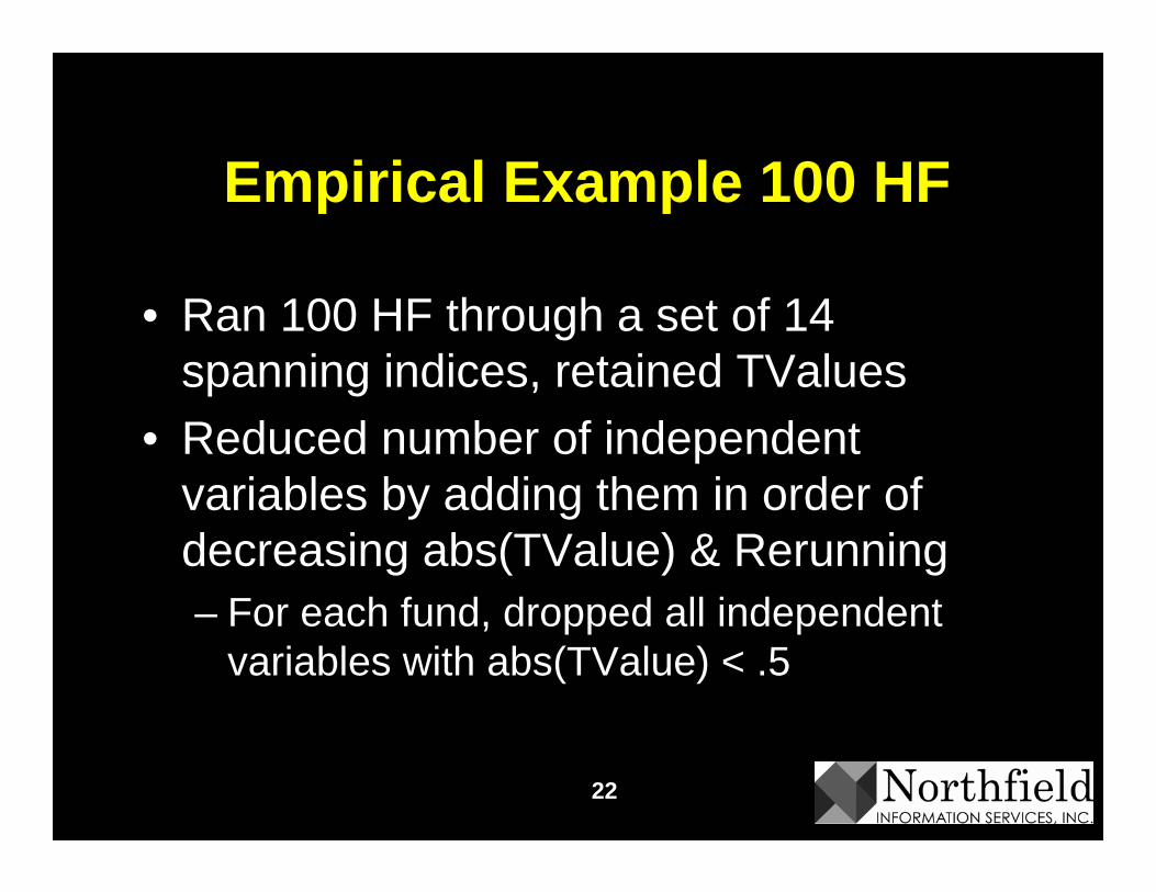
Empirical Example 100 HF

• Ran 100 HF through a set of 14 spanning indices, retained TValues

• Reduced number of independent variables by adding them in order of decreasing abs(TValue) & Rerunning– For each fund, dropped all independent

variables with abs(TValue) < .5

23

Style Analysis Results

• R2 between .005 and .9, averaging about .36

• Interesting trend: the greater Cash Allocation, the lower the R2:– The more “hedged” the fund, the less

information there is for the style analysis to pick up on…

24

%Cash Allocation vs Style R2

0

20

40

60

80

100

120

0 0.2 0.4 0.6 0.8 1

R2

% C

ash

Allo

catio

n

Series1

R2 = .465

25

Next Step (Empirical Ex. Cont)

• Combined spanning index constituents according to style weights, used result as benchmark, optimized, max 500 assets.

• Harvested resultant expected standard deviation of returns.

• Calculated historic standard deviation of HF returns.

26

Modelled Vs Realized Risk

0

2

4

6

8

10

12

14

16

18

0 5 10 15 20 25

HF realized risk

MF

E[ris

k]

Hisoric HF risk

27

Results

• Slope = .978• R2 = .486• 85% of the modeled portfolio risks were

smaller than the respective observed HF risks.

28

Empirical Conclusions

• The Style Analysis does a good job of modeling a Hedge Fund’s Factor Variance.

• A further adjustment of stock specific is required to beef up the Expected Risks to fit.– This can be done by iteratively adjusting:

• UnsysRAP• MaxAssets

How Large is the Equity Premium Today?

June 8, 2007

Samuel ThompsonPartner, Research

Arrowstreet Capital, LP

1

The equity premium

• The equity premium is the expected excess return on a broad stock index over a safe bond market investment

• To measure it, we need to make choices:– What stock index? (I will emphasize the World index but also

show results for the US and Canada)– What safe investment? (I will use long-term inflation-indexed

bonds)– What starting point? (I will use current conditions)– What investment horizon? (I will discuss forecasting methods

suitable for a 5-10 year holding period)– What kind of expectation? (I will use a geometric average)

2

Key questions

• Do we believe that the equity premium has declined since 1950?– If so, then the historical mean return over-states future returns

• Do we believe in mean reversion? Price-earnings ratios are at historically high levels. Do we think they will fall?– If we believe in mean reversion, then we should be extremely

pessimistic about stock market returns over the next five years– If we do not believe in mean reversion, then regression-based

forecasts of the equity premium are overly pessimistic

• Corporate profits are at historical highs. Do we believe they will remain high?

3

Alternative ways to estimate the equity premium

Two extreme approaches: 1. Take an average of historically realized excess returns.2. Estimate the historical relationship between realized

excess returns and valuation ratios. Example: regress returns on the earnings yield.

I prefer two compromise approaches: 3. Adjust historical averages to reflect the decline in market

valuation ratios. 4. Predict the equity premium with valuation ratios. Use

logic rather than historical statistics to determine the predictive model.

4

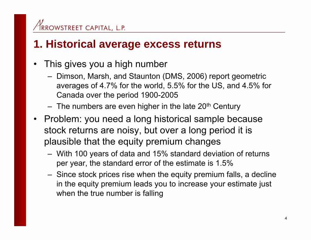
1. Historical average excess returns

• This gives you a high number– Dimson, Marsh, and Staunton (DMS, 2006) report geometric

averages of 4.7% for the world, 5.5% for the US, and 4.5% for Canada over the period 1900-2005

– The numbers are even higher in the late 20th Century

• Problem: you need a long historical sample because stock returns are noisy, but over a long period it is plausible that the equity premium changes– With 100 years of data and 15% standard deviation of returns

per year, the standard error of the estimate is 1.5%– Since stock prices rise when the equity premium falls, a decline

in the equity premium leads you to increase your estimate just when the true number is falling

5

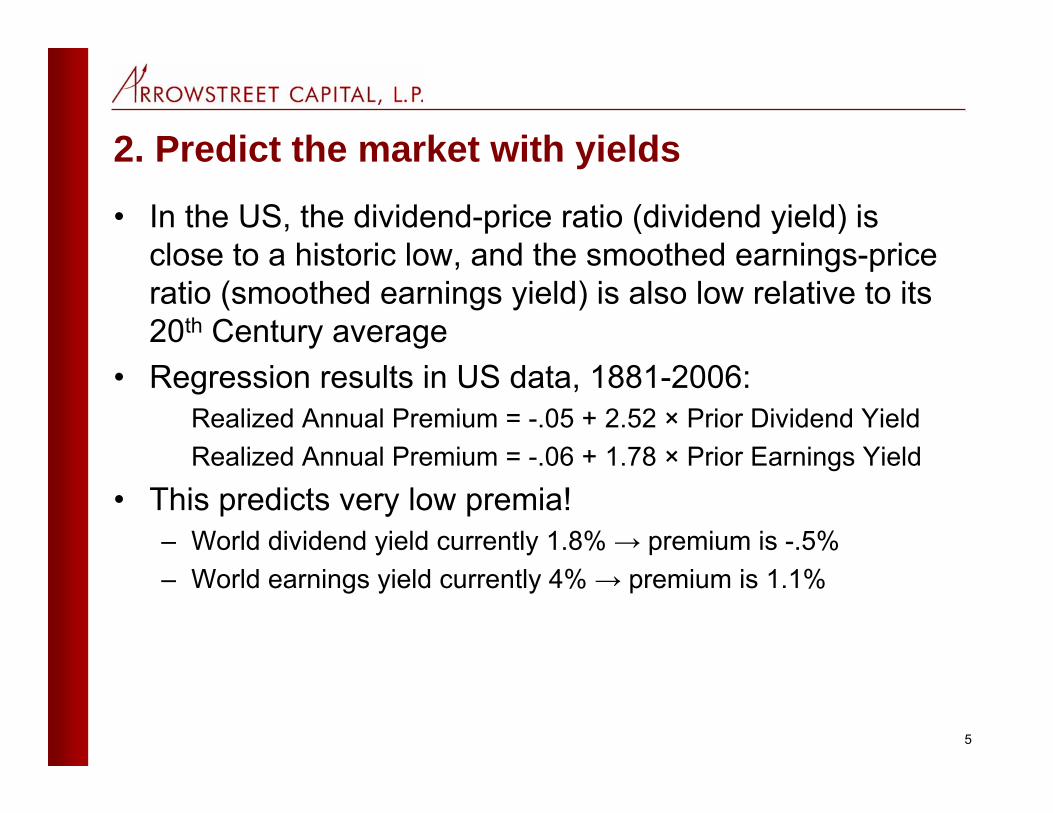
2. Predict the market with yields

• In the US, the dividend-price ratio (dividend yield) is close to a historic low, and the smoothed earnings-price ratio (smoothed earnings yield) is also low relative to its 20th Century average

• Regression results in US data, 1881-2006:Realized Annual Premium = -.05 + 2.52 × Prior Dividend YieldRealized Annual Premium = -.06 + 1.78 × Prior Earnings Yield

• This predicts very low premia!– World dividend yield currently 1.8% → premium is -.5%– World earnings yield currently 4% → premium is 1.1%

6

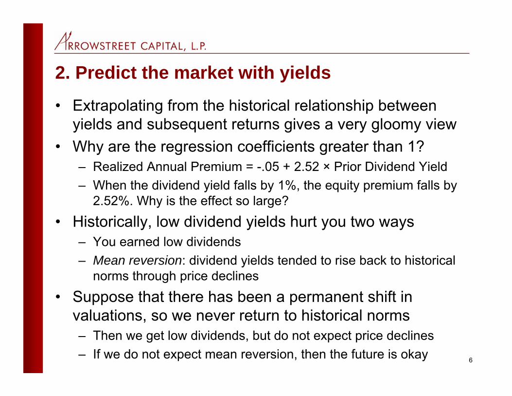
2. Predict the market with yields

• Extrapolating from the historical relationship between yields and subsequent returns gives a very gloomy view

• Why are the regression coefficients greater than 1?– Realized Annual Premium = -.05 + 2.52 × Prior Dividend Yield– When the dividend yield falls by 1%, the equity premium falls by

2.52%. Why is the effect so large?

• Historically, low dividend yields hurt you two ways– You earned low dividends– Mean reversion: dividend yields tended to rise back to historical

norms through price declines

• Suppose that there has been a permanent shift in valuations, so we never return to historical norms– Then we get low dividends, but do not expect price declines– If we do not expect mean reversion, then the future is okay

7

S&P 500 10-Year Average Dividend/ Price

0.00%

2.00%

4.00%

6.00%

8.00%

10.00%

12.00%

14.00%

16.00%

18.00%

1881 1901 1921 1941 1961 1981 2001

Year

Div

iden

d-Pr

ice

Rat

io

Average D/P = 4.4%

D/P in 1/06 = 1.69%

``

8

1.7% in 2006 Historical average

Low 1973 D/P followed by price declines

9

Two flawed approaches

• The equity premium may have fallen• When the equity premium falls, the historical mean

becomes unreasonably bullish• When the equity premium falls, forecasts based on the

historical relationship between returns and yields become unreasonably bearish

• What I advocate: use yields to forecast the equity premium, but do not assume mean reversion. Low dividend yields mean low dividends, but do not mean that prices will collapse

10

3. Adjusting the historical average

• DMS and Fama-French (2002) propose the following:• Historical average returns:

Avgstock returns = Avgdividend yield + Avgprice growth

• Adjusted estimate:Avgstock returns = Avgdividend yield + Avgearnings growth

• What’s the idea?– If the equity premium falls, historical price growth will be higher

than in the future. Historical earnings growth will not be similarly overstated

– Suppose that the price-earnings ratio is expected to be stable (so no mean reversion). Then going forward, average price growth equals average earnings growth

– We estimate price growth going forward by averaging over historical earnings growth

11

3. Adjusting the historical average

• Adjustment to the 1900-2005 average returns give us a geometric equity premium of 4.0% for the world, 4.8% for the US, 3.5% for Canada– This adjustment lowers the historical average by about 0.7% in the US

and globally, and about 1% in Canada

• We can further adjust the estimate using today’s dividend yield:– Avgstock returns = Today’s dividend yield + Avgearnings growth– This adjustment leads to a geometric equity premium of 2.5% for

the world, 3.3% for the US, 2% for Canada

• The adjustments lead to lower but still sizeable equity premiums

12

4. Steady-state valuation models

• The simplest steady-state model is the Gordon growth model: R = D/P + G

• That is, returns come from income and capital gains, which in steady state must equal dividend growth

• Use current D/P and an estimate of G to infer R • The problem with this is that US firms have shifted from

dividends to share repurchases, which has altered G in a way that is hard to estimate

• Campbell and Thompson (2006) find that an earnings-based approach works better

13

4. Steady-state valuation models• Use two facts:

– D/P = (D/E)(E/P)– G = (1-D/E) ROE, where ROE is accounting return on

equity• Get an earnings-based formula:

– R = (D/E)(E/P) + (1-D/E) ROE• The rate of return is a weighted average of the earnings

yield and profitability, where the payout ratio is the weight on the earnings yield

• In practice, you need to smooth earnings, ROE, and payout ratio to eliminate short-run cyclical noise

• Finally, to get an equity premium number you must subtract an estimate of the real interest rate

14

4. Steady-state valuation models• Steady-state approach vs. regression

– Assume that ROE = E/P. The steady-state prediction isR = E/P

– Recall the regression results:R = -.06 + 1.78 × E/P

– The steady state approach over-rules the regression coefficients of -.06 and 1.78 with 0 and 1.

• The steady-state approach uses logic rather than historical statistics to determine the relationship between valuation and future stock returns

• The steady-state approach assumes no mean reversion• Campbell and Thompson (2006) find that in historical

data the steady-state approach leads to more accurate stock forecasts than regression-based approaches

15

Earnings yield

0.0

5.1

.15

.2

1982 1986 1990 1994 1998 2002 2006

World US Canada

3-Year Smoothed Earnings / Current Price

16

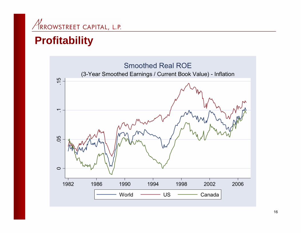
Profitability0

.05

.1.1

5

1982 1986 1990 1994 1998 2002 2006

World US Canada

(3-Year Smoothed Earnings / Current Book Value) - InflationSmoothed Real ROE

17

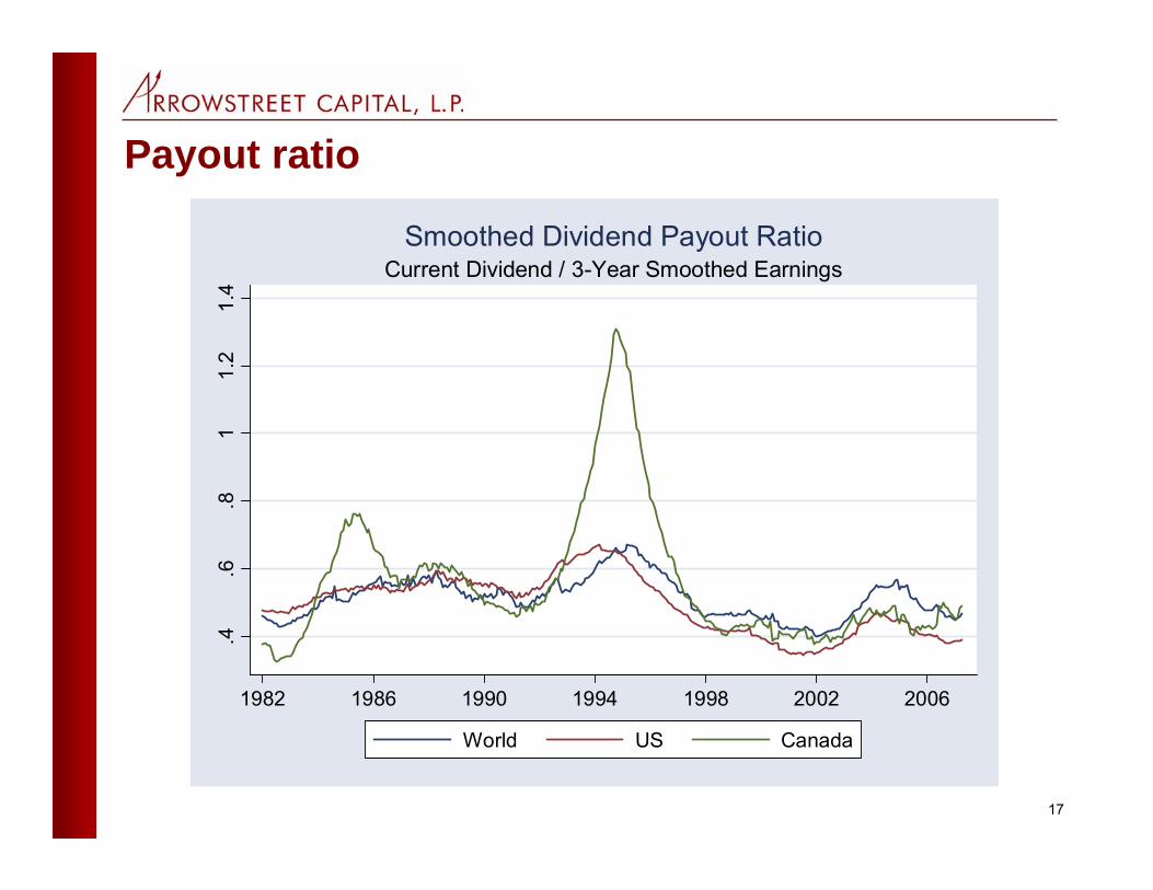
Payout ratio.4

.6.8

11.

21.

4

1982 1986 1990 1994 1998 2002 2006

World US Canada

Current Dividend / 3-Year Smoothed EarningsSmoothed Dividend Payout Ratio

18

Real interest rate

.01

.02

.03

.04

.05

1982 1986 1990 1994 1998 2002 2006

UK US

Inflation-Indexed Government Bond Yields

19

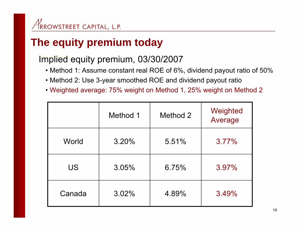
The equity premium today•Point estimates Implied equity premium, 03/30/2007

• Method 1: Assume constant real ROE of 6%, dividend payout ratio of 50%• Method 2: Use 3-year smoothed ROE and dividend payout ratio• Weighted average: 75% weight on Method 1, 25% weight on Method 2

3.49%4.89%3.02%Canada

3.97%6.75%3.05%US

3.77%5.51%3.20%World

Weighted AverageMethod 2Method 1

20

Implied world equity premium-.0

20

.02

.04

.06

.08

1982 1986 1990 1994 1998 2002 2006

Assume Constant Real ROE 6%, Dividend Payout Ratio 50%Use 3-Year Smoothed ROE and Dividend Payout Ratio

Equity Premium -- World

21

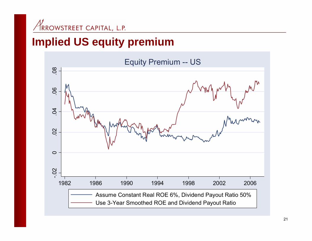
Implied US equity premium-.0

20

.02

.04

.06

.08

1982 1986 1990 1994 1998 2002 2006

Assume Constant Real ROE 6%, Dividend Payout Ratio 50%Use 3-Year Smoothed ROE and Dividend Payout Ratio

Equity Premium -- US

22

Implied Canada equity premium-.0

20

.02

.04

.06

.08

1982 1986 1990 1994 1998 2002 2006

Assume Constant Real ROE 6%, Dividend Payout Ratio 50%Use 3-Year Smoothed ROE and Dividend Payout Ratio

Equity Premium -- Canada

23

The world equity premium today

• The steady-state approach gives results that are highly sensitive to one’s beliefs about corporate profitability

• If recent profitability is sustainable, with a high reinvestment rate, then the world equity premium is 5.51%

• If profitability and reinvestment rates return to their late 20th Century averages, then the world equity premium is only 3.20%

• A reasonable compromise number is 3.8% • This is almost one percentage point lower than the 1900-

2005 historical average reported by DMS• Note that the equity premium is this high only because

long-term real interest rates are low

24

The equity premium in the US and Canada

• The US numbers are even more sensitive to the assumption about profitability. In Canada the recent profit boom is smaller, so profit sustainability is less important

• In the US, the compromise number of 4% is 1.5% below the 1900-2005 historical average

• In Canada, the compromise number of 3.5% is 1% below the 1900-2005 historical average

• Thus in the US and Canada, we should not expect the future to be as good as the past

• Reality check: Graham and Harvey (2007) survey CFO’s of US corporations and report a premium of 3.4%

25

Conclusion• Sensible methods for estimating the equity premium give

– Positive, significant numbers – World forecasts are 3.8% today versus 4.7% historically– If corporate profitability reverts to long run averages, the world

premium falls to 3.2%.– Absolute returns will be lower still: real interest rates are about

2% today versus 3.5% in the 1990s

• If we believe in mean reversion, we become very pessimistic. In the past, rising earnings yields have come from falling prices

• If equities have been permanently revalued, then we are much less pessimistic

Instinet Algorithms – Wizard

Implied Risk Acceptance Parameters in the Execution of

Institutional Equity TradesThorsten Schmidt, CFA

Northfield Summer SeminarNewport, RIJune 8, 2007

2

OverviewOverview

Objective• Assess the risk-aversion implicit in the execution of

institutional tradesMethodology• Generate implied RAPs from Instinet’s database of

institutional tradesSample• 21,959 institutional orders between 10/1/06 and 4/20/07

3

MethodologyMethodology

Sample Characteristics• Algorithmic trade executions• Orders without limits (avoid selection biases)• Fully completed ordersGrouping• We utilize 3 different strategies which are chosen by the

trader as a proxy for the level of risk aversion• These strategies are distinct in terms of the amount of

market risk associated with them

4

Methodology (cont’d)Methodology (cont’d)

Results Measurement• We use ‘implementation shortfall,’ i.e. difference b/w

volume-weighted execution price and last market print at order arrival

Order Strategy Groupings• Volume Participation*: Most aggressive trading style,

least market risk exposure• Implementation Shortfall (“Wizard”): Medium aggressive

trading style, medium market risk exposure• VWAP: Most passive trading style, highest market risk

exposure

* Avg Volume Participation Rate is 26%

5

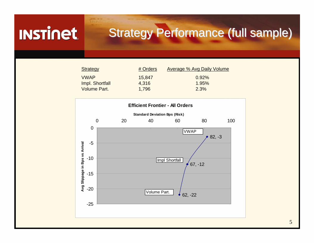
Strategy Performance (full sample)Strategy Performance (full sample)

Strategy # Orders Average % Avg Daily Volume

VWAP 15,847 0.92%Impl. Shortfall 4,316 1.95%Volume Part. 1,796 2.3%

Efficient Frontier - All Orders

62, -22

67, -12

82, -3

-25

-20

-15

-10

-5

00 20 40 60 80 100

Standard Deviation Bps (Risk)

Avg

Slip

page

in B

ps v

s A

rriv

al

VWAP

Impl Shortfall

Volume Part.

6

Utility EvaluationUtility Evaluation

Utility (Northfield Definition)

U = alpha – [STE^2/SYSRAP + UTE^2/URAP] – Cost –Penalties

Utility (adapted for this analysis)

U = ( 0 – [StdDev1^2 / SYSRAP/100] – abs(Slippage1) ) * 100

Note• Because institutional trade executions lose money on average, the utility will always be negative• We are trying to minimize disutility 1 Expressed in decimal format

7

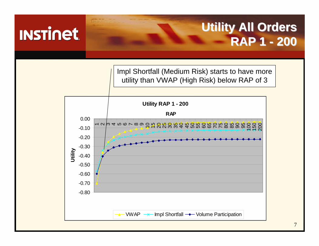
Utility All Orders Utility All Orders RAP 1 RAP 1 -- 200200

Utility RAP 1 - 200

-0.80

-0.70

-0.60

-0.50

-0.40

-0.30

-0.20

-0.10

0.00

1 2 3 4 5 6 7 8 9 10 15 20 25 30 35 40 45 50 55 60 65 70 75 80 85 90 95 100

150

200

RAP

Util

ity

VWAP Impl Shortfall Volume Participation

Impl Shortfall (Medium Risk) starts to have more utility than VWAP (High Risk) below RAP of 3

8

Utility All Orders Utility All Orders below RAP 1below RAP 1

Utility RAP 0.1 - 1

-8.00

-7.00-6.00

-5.00-4.00

-3.00

-2.00-1.00

0.00

0.1

0.2

0.3

0.4

0.5

0.6

0.7

0.8

0.9 1

RAP

Util

ity

VWAP Impl Shortfall Volume Participation

Volume Participation, as typically utilized* (Low Risk) is the strategy with the most utility only below

RAP of 0.7 ! Is anyone this risk averse?

* Avg Volume Participation Rate is 26%

9

StrategyStrategy Performance Performance (< 2% ADV)(< 2% ADV)

Strategy # Orders Average % Avg Daily Volume

VWAP 14,115 0.4%Impl. Shortfall 2,977 0.6%Volume Part. 1,283 0.7%

Efficient Frontier - 0% to <2% ADV

75, -2

63, -7

38, -13-14

-12

-10

-8

-6

-4

-2

00 20 40 60 80

Standard Deviation Bps (Risk)

Avg

Slip

page

in B

ps v

s A

rriv

al

Impl Shortfall

Volume Part.

VWAP

Among orders ADV <2%, Impl Shortfall does not show a strong comparative advantage

10

<2% ADV, Utility RAP 1 - 200

-0.70

-0.60

-0.50

-0.40

-0.30

-0.20

-0.10

0.00

1 2 3 4 5 6 7 8 9 10 15 20 25 30 35 40 45 50 55 60 65 70 75 80 85 90 95 100

150

200

RAP

Util

ity

VWAP Impl Shortfall Volume Participation

Utility (<2% ADV) Utility (<2% ADV) RAP 1 RAP 1 -- 200200

For ADV < 2%, Volume Participation becomes strategy with most utility at RAP 3 and below b/c of lower potential to ‘do damage’ with smaller orders

11

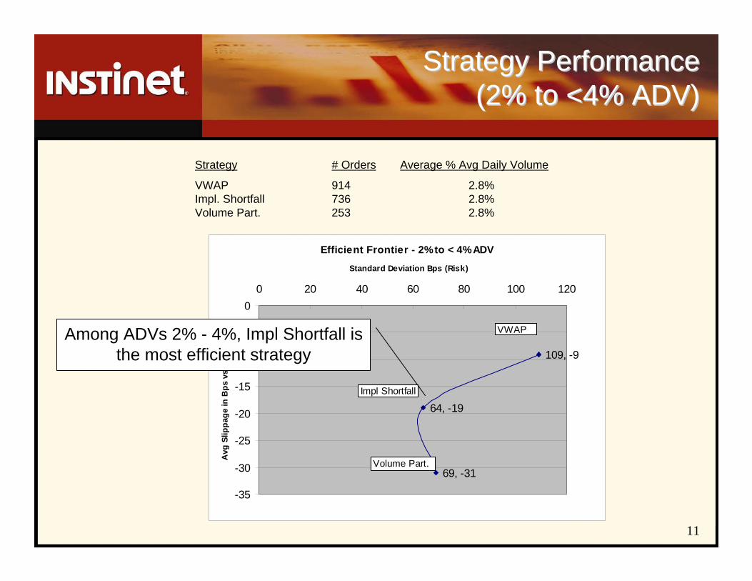
Strategy Performance Strategy Performance (2% to <4% ADV)(2% to <4% ADV)

Strategy # Orders Average % Avg Daily Volume

VWAP 914 2.8%Impl. Shortfall 736 2.8%Volume Part. 253 2.8%

Efficient Frontier - 2% to < 4% ADV

109, -9

64, -19

69, -31

-35

-30

-25

-20

-15

-10

-5

00 20 40 60 80 100 120

Standard Deviation Bps (Risk)

Avg

Slip

page

in B

ps v

s A

rriv

al

VWAP

Impl Shortfall

Volume Part.

Among ADVs 2% - 4%, Impl Shortfall is the most efficient strategy

12

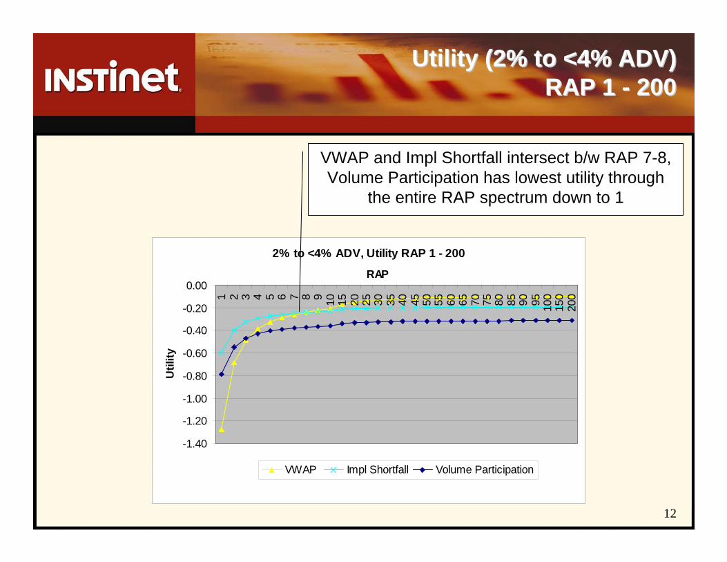
Utility (2% to <4% ADV) Utility (2% to <4% ADV) RAP 1 RAP 1 -- 200200

2% to <4% ADV, Utility RAP 1 - 200

-1.40

-1.20

-1.00

-0.80

-0.60

-0.40

-0.20

0.00

1 2 3 4 5 6 7 8 9 10 15 20 25 30 35 40 45 50 55 60 65 70 75 80 85 90 95 100

150

200

RAP

Util

ity

VWAP Impl Shortfall Volume Participation

VWAP and Impl Shortfall intersect b/w RAP 7-8, Volume Participation has lowest utility through

the entire RAP spectrum down to 1

13

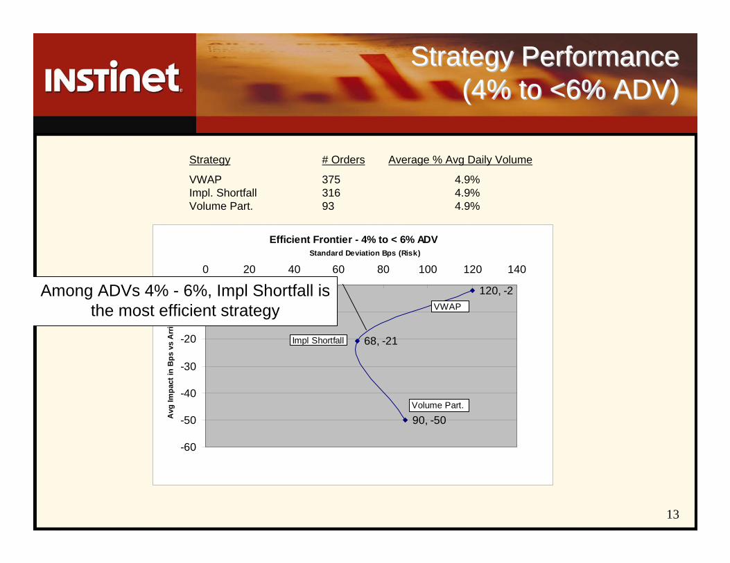
Strategy Performance Strategy Performance (4% to <6% ADV)(4% to <6% ADV)

Strategy # Orders Average % Avg Daily Volume

VWAP 375 4.9%Impl. Shortfall 316 4.9%Volume Part. 93 4.9%

Efficient Frontier - 4% to < 6% ADV

120, -2

68, -21

90, -50

-60

-50

-40

-30

-20

-10

00 20 40 60 80 100 120 140

Standard Deviation Bps (Risk)

Avg

Impa

ct in

Bps

vs

Arr

ival

VWAP

Impl Shortfall

Volume Part.

Among ADVs 4% - 6%, Impl Shortfall is the most efficient strategy

14

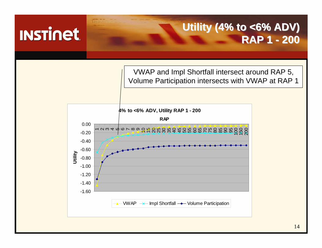
Utility (4% to <6% ADV) Utility (4% to <6% ADV) RAP 1 RAP 1 -- 200200

4% to <6% ADV, Utility RAP 1 - 200

-1.60

-1.40

-1.20

-1.00

-0.80

-0.60

-0.40

-0.20

0.00

1 2 3 4 5 6 7 8 9 10 15 20 25 30 35 40 45 50 55 60 65 70 75 80 85 90 95 100

150

200

RAP

Util

ity

VWAP Impl Shortfall Volume Participation

VWAP and Impl Shortfall intersect around RAP 5, Volume Participation intersects with VWAP at RAP 1

15

Summary• A lot of trade executions performed at implied RAPs <10,

and even at RAP <1• Most balanced institutional portfolios have RAPs of 50-75

(rule of thumb: desired tracking error * 6)

Why are many institutional trades this risk averse?• Short-term alpha• Workflow reasons (get done and move on)• Psychology of trader-PM relationship

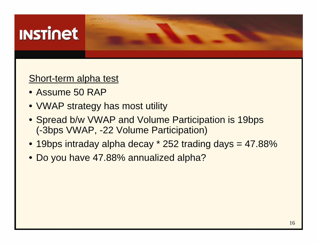
16

Short-term alpha test• Assume 50 RAP• VWAP strategy has most utility• Spread b/w VWAP and Volume Participation is 19bps

(-3bps VWAP, -22 Volume Participation) • 19bps intraday alpha decay * 252 trading days = 47.88% • Do you have 47.88% annualized alpha?

17

Conclusions• The reasons for low implied RAPs are structural and

behavioral• Rigorous analysis of trading performance can shed light on

implied RAPs of executions• It can help align the RAPs of your trading with those of

your portfolio• Talk to your broker (e.g. Instinet) to help you do this

18

Thorsten Schmidt, CFAFVP Algorithmic Trading

thorsten.schmidt@instinet.com

Tel 212.310.4177

19

This presentation is for information purposes only and does not constitute an offer, solicitation, or recommendation with respect to the purchase or sale of

any security. System response times may vary for a number of reasons, including market conditions, trading volumes and system performance.

© 2007 Instinet, LLC. All rights reserved. INSTINET is a registered mark. Instinet, LLC, member NASD/SIPC.

Alpha Scaling RevisitedAlpha Scaling Revisited

June 8, 2007June 8, 2007

Anish R. Shah, CFAAnish R. Shah, CFANorthfield Information ServicesNorthfield Information Services

Anish@northinfo.comAnish@northinfo.com

The GoalThe Goal

One way One way -- fit a linear modelfit a linear modelŷŷ((ĝĝ) = ) = AA ĝĝ + + bb

Minimizing expected squared error,Minimizing expected squared error,ŷŷ((ĝĝ) = ) = E(E(yy) + ) + cov(cov(yy, , gg) ) cov(cov(gg, , gg))--11 [[ĝĝ –– E(E(gg)])]

End of presentationEnd of presentation

A procedure that forecasts A procedure that forecasts variable(svariable(s) ) yy from signals from signals gg

ForecastingMachine

Signalsĝ

Forecastsŷ

The Real GoalThe Real Goal

Additional considerationsAdditional considerationsoptimizers seek extremes (by mandate!)optimizers seek extremes (by mandate!)all forecasts have errorall forecasts have erroroptimized selection introduces biasoptimized selection introduces bias

Most forecasting methods, e.g. Most forecasting methods, e.g. GrinoldGrinold formula, address the 1formula, address the 1stst half. half. This talk focuses on the 1This talk focuses on the 1stst halfhalf

Shrinking all forecasts towards the average forecast across secuShrinking all forecasts towards the average forecast across securities, rities, for example, is one way to deal with the 2for example, is one way to deal with the 2ndnd halfhalf

The 1The 1stst is about forecasting, the 2is about forecasting, the 2ndnd about optimizing with errorsabout optimizing with errors

Build forecasts that are suitable for optimizationBuild forecasts that are suitable for optimization

ForecastingMachineSignals Forecasts Conditioner Optimizable

Forecasts

More About The DifferenceMore About The Difference

Forecasting returns for many stocks from a set of signalsForecasting returns for many stocks from a set of signals

In basic linear model, each forecast is constructed separatelyIn basic linear model, each forecast is constructed separatelyŷ(ĝ) = E(y) + cov(y, g) cov(g, g)-1 [ĝ – E(g)]

ŷŷ((ĝĝ) = [) = [ŷŷ11((ĝĝ), ), ŷŷ22((ĝĝ)), , …… ]]TT

ŷŷkk((ĝĝ) = ) = E(yE(ykk) + ) + cov(ycov(ykk, , gg) ) cov(cov(gg, , gg))--11 [[ĝĝ –– E(E(gg)])]

So, stock 1’s forecast is concerned with signals that affect stoSo, stock 1’s forecast is concerned with signals that affect stock 2 to ck 2 to the extent that those signals also affect stock 1. It is not atthe extent that those signals also affect stock 1. It is not at all all concerned with the final forecast for stock 2concerned with the final forecast for stock 2

In contrast, portfolio optimization compares securities against In contrast, portfolio optimization compares securities against each each other and cares only about relative valueother and cares only about relative value

Articulate So Formulas Make SenseArticulate So Formulas Make Sense

Say what the signals areSay what the signals aree.g. e.g. ggii == stock stock i’si’s raw alpha forecastraw alpha forecast

stock stock i’si’s most recent earnings surprisemost recent earnings surprisestock stock i’si’s crosscross--sectional ranksectional rankchange in 90 day Tchange in 90 day T--bill yieldbill yield

Say what you are forecastingSay what you are forecastinge.g. e.g. yykk == stock stock k’sk’s returnreturn

stock stock k’sk’s return return –– market returnmarket returnstock stock k’sk’s return net of market β and industryreturn net of market β and industrystock stock k’sk’s stock specific returnstock specific return

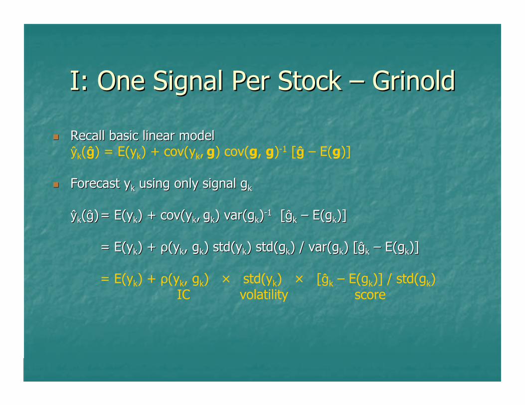
I: One Signal Per Stock I: One Signal Per Stock –– GrinoldGrinold

Recall basic linear modelRecall basic linear modelŷk(ĝ) = E(yk) + cov(yk, g) cov(g, g)-1 [ĝ – E(g)]

Forecast Forecast yykk using only signal using only signal ggkk

ŷŷkk((ĝĝ))= = E(yE(ykk) + ) + cov(ycov(ykk,, ggkk) var(g) var(gkk))--11 [[ĝĝkk –– E(gE(gkk)])]

= = E(yE(ykk) + ) + ρρ((yykk, , ggkk) ) std(ystd(ykk) ) std(gstd(gkk) / ) / var(gvar(gkk) [) [ĝĝkk –– E(gE(gkk)])]

= E(yk) + ρ(yk, gk) × std(yk) × [ĝk – E(gk)] / std(gk)IC volatility score

I: I: GrinoldGrinold –– No Confusion About No Confusion About ParametersParameters

IC = correlation (signal, return being forecast)IC = correlation (signal, return being forecast)

Volatility is the volatility of the return being forecastVolatility is the volatility of the return being forecast

Score is the zScore is the z--score of that instance of the signalscore of that instance of the signal

IC can be estimated over a group of securities (e.g. same IC can be estimated over a group of securities (e.g. same cap/industry/volatility) if the model works equally well on themcap/industry/volatility) if the model works equally well on them

Likewise, you would expect lower IC’s for volatile securities (hLikewise, you would expect lower IC’s for volatile securities (harder arder to predict) than for less volatile ones (easier to predict.) A to predict) than for less volatile ones (easier to predict.) A single IC single IC exaggerates volatile securities’ alphasexaggerates volatile securities’ alphas

I: I: GrinoldGrinold ExampleExample

The upcoming period isThe upcoming period isgood for DELL (zgood for DELL (z--score of 1) score of 1) better for MSFT (zbetter for MSFT (z--score of 2)score of 2)great for PEP (zgreat for PEP (z--score of 3)score of 3)

StockStock--specific volatility: specific volatility: σσssssDELLDELL = 27%, = 27%, σσssss

MSFTMSFT = 25%, = 25%, σσssssPEPPEP = 9%= 9%

Skill, Skill, corrcorr(signal,return(signal,return)): : ICICtechtech = .10, = .10, ICICconsumerconsumer = .15= .15

Assume Assume E[yE[y] = 0, stock] = 0, stock--specific return averages 0 over timespecific return averages 0 over time

ŷŷDELLDELL = 0 + .10 = 0 + .10 ×× 27% 27% ×× 1 = 2.7%1 = 2.7%ŷŷMSFTMSFT = 0 + .10 = 0 + .10 ×× 25% 25% ×× 2 = 5.0%2 = 5.0%ŷŷPEPPEP = 0 + .15 = 0 + .15 ×× 9% 9% ×× 3 = 4.0%3 = 4.0%

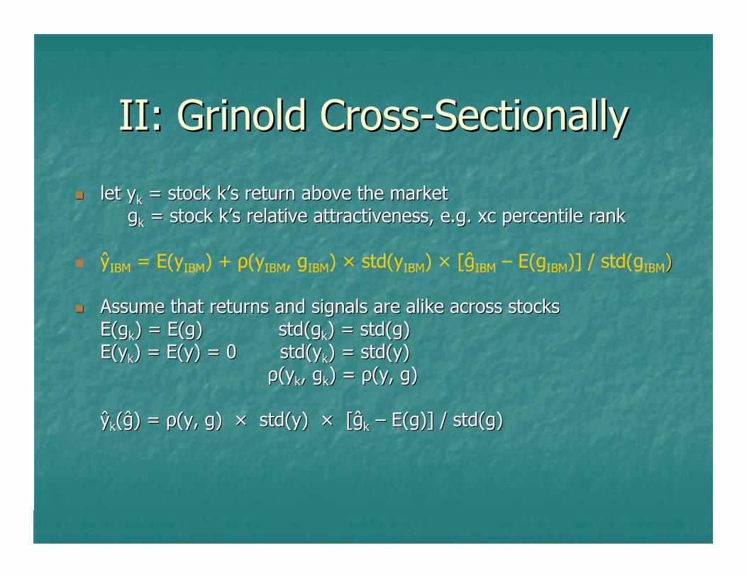
II: II: GrinoldGrinold CrossCross--SectionallySectionally

let let yykk = stock = stock k’sk’s return above the marketreturn above the marketggkk = stock = stock k’sk’s relative attractiveness, e.g. relative attractiveness, e.g. xcxc percentile rankpercentile rank

ŷIBM = E(yIBM) + ρ(yIBM, gIBM) × std(yIBM) × [ĝIBM – E(gIBM)] / std(gIBM))

Assume that returns and signals are alike across stocksAssume that returns and signals are alike across stocksE(gE(gkk) = ) = E(gE(g)) std(gstd(gkk) = ) = std(gstd(g))E(yE(ykk) = ) = E(yE(y) = 0) = 0 std(ystd(ykk) = ) = std(ystd(y))

ρ(yρ(ykk, , ggkk) = ) = ρ(yρ(y, g), g)

ŷŷkk(ĝ(ĝ) = ) = ρ(yρ(y, g) × , g) × std(ystd(y) × [) × [ĝĝkk –– E(gE(g)] / )] / std(gstd(g))

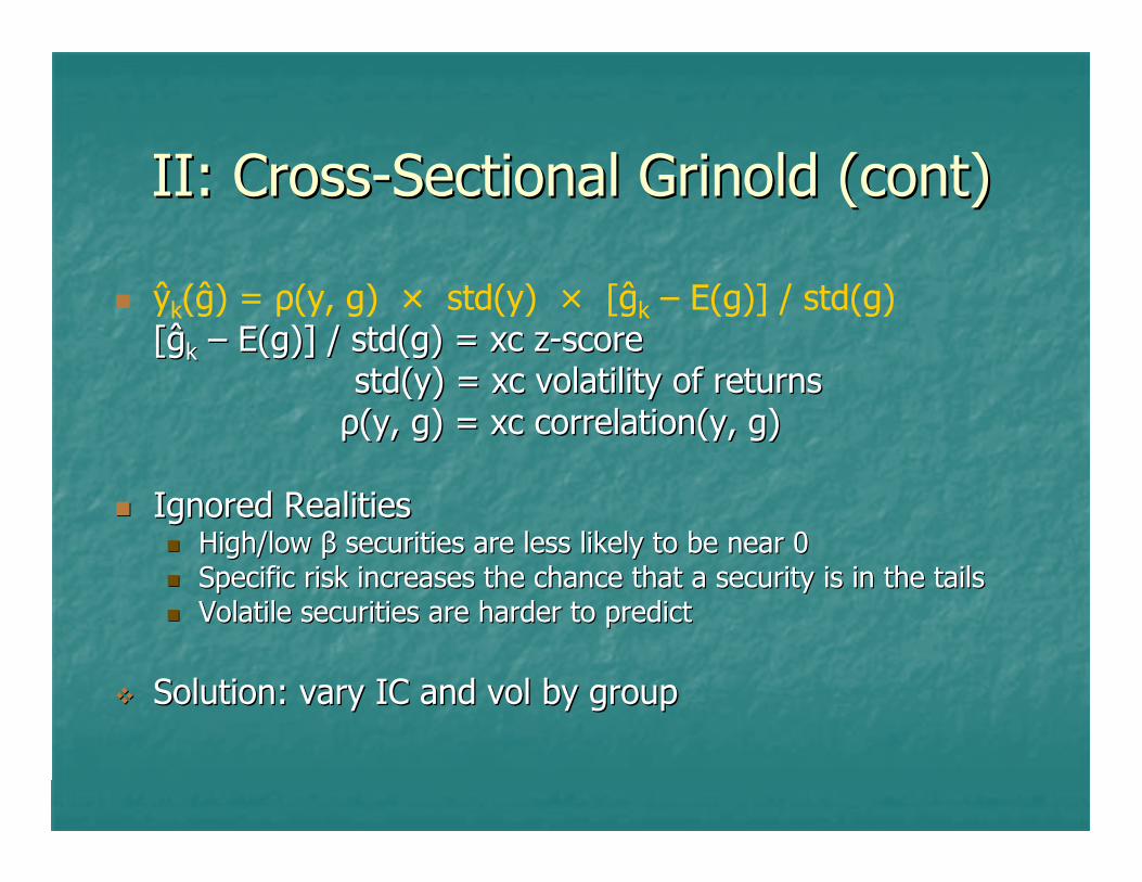
II: CrossII: Cross--Sectional Sectional GrinoldGrinold (cont)(cont)

ŷk(ĝ) = ρ(y, g) × std(y) × [ĝk – E(g)] / std(g)[[ĝĝkk –– E(gE(g)] / )] / std(gstd(g) ) = = xcxc zz--scorescore

std(ystd(y) ) = = xcxc volatility of returnsvolatility of returnsρ(yρ(y, g) , g) = = xcxc correlation(ycorrelation(y, g), g)

Ignored RealitiesIgnored RealitiesHigh/low β securities are less likely to be near 0High/low β securities are less likely to be near 0Specific risk increases the chance that a security is in the taiSpecific risk increases the chance that a security is in the tailslsVolatile securities are harder to predictVolatile securities are harder to predict

Solution: vary IC and Solution: vary IC and volvol by groupby group

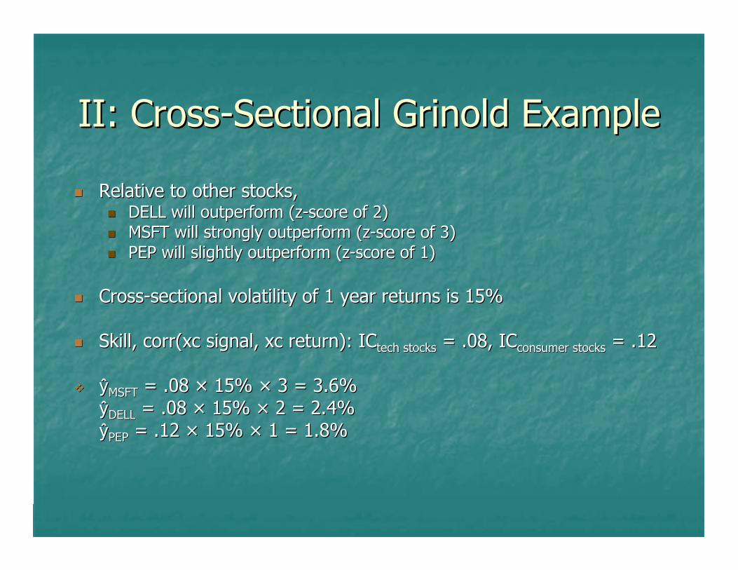
II: CrossII: Cross--Sectional Sectional GrinoldGrinold ExampleExample

Relative to other stocks,Relative to other stocks,DELL will outperform (zDELL will outperform (z--score of 2) score of 2) MSFT will strongly outperform (zMSFT will strongly outperform (z--score of 3)score of 3)PEP will slightly outperform (zPEP will slightly outperform (z--score of 1)score of 1)

CrossCross--sectional volatility of 1 year returns is 15%sectional volatility of 1 year returns is 15%

Skill, Skill, corrcorr(xc(xc signal, signal, xcxc return)return): : ICICtechtech stocksstocks = .08, = .08, ICICconsumerconsumer stocksstocks = .12= .12

ŷŷMSFTMSFT = .08 = .08 ×× 15% 15% ×× 3 = 3.6%3 = 3.6%ŷŷDELLDELL = .08 = .08 ×× 15% 15% ×× 2 = 2.4%2 = 2.4%ŷŷPEPPEP = .12 = .12 ×× 15% 15% ×× 1 = 1.8%1 = 1.8%

III: Bayesian ApproachIII: Bayesian ApproachBlackBlack--LittermanLitterman

Motivated by need to stabilize asset allocation optimizationMotivated by need to stabilize asset allocation optimization

Assume a prior distribution on the vector of mean returnsAssume a prior distribution on the vector of mean returnsCentered at implied alpha that makes market portfolio optimal Centered at implied alpha that makes market portfolio optimal (stability)(stability)Covariance is proportional to covariance of returnsCovariance is proportional to covariance of returns

New information given as portfolio forecasts with errorNew information given as portfolio forecasts with errorIBMIBM’’s return is 5% s return is 5% ±± 2%2%i.e. return of portfolio holding 100% IBM is 5% i.e. return of portfolio holding 100% IBM is 5% ±± 2%2%

MSFT will outperform IBM by 3% MSFT will outperform IBM by 3% ±± 4%4%i.e. return of portfolio long MSFT short IBM is 3% i.e. return of portfolio long MSFT short IBM is 3% ±± 4%4%

Combined forecast is expected value given prior and informationCombined forecast is expected value given prior and information

III: BlackIII: Black--LittermanLitterman (cont)(cont)prior on mean returns:prior on mean returns:mm ~ N(~ N(mm00, , ΣΣ00))

forecasts impart new information:forecasts impart new information:ĝĝ = = PP E[E[mm | info] + | info] + εεεε ~ N(~ N(00, , ΩΩ))

ŷŷ = [= [ΣΣ00--11 + + PPTTΩΩ--11PP]]--11 [[ΣΣ00

--1 1 mm00 + + PPTTΩΩ--11ĝĝ]]= = mm00 + [+ [ΣΣ00

--11 + + PPTTΩΩ--11PP]]--1 1 PPTTΩΩ--11 ((ĝĝ –– PmPm00))

= = mm00 + [+ [ΣΣ00 –– ((PPΣΣ00))TT((ΩΩ + + PPΣΣ00PPTT))--1 1 PPΣΣ00] ] PPTTΩΩ--11 ((ĝĝ –– PmPm00))

Because of the priorBecause of the prior’’s covariance, one security tells us about another. s covariance, one security tells us about another. e.g. if IBM and DELL are correlated, information about IBM sayse.g. if IBM and DELL are correlated, information about IBM sayssomething about DELLsomething about DELL

Note: Holding the benchmark in benchmark relative optimization Note: Holding the benchmark in benchmark relative optimization implies an alpha of 0 for all securitiesimplies an alpha of 0 for all securities

III: BlackIII: Black--LittermanLitterman ExampleExample

Prior on IBM and DELL of (2%, 5%), with Prior on IBM and DELL of (2%, 5%), with respective variances 4%respective variances 4%22, 9%, 9%22 and correlation and correlation .5.5

Predict that IBM will return 5% ± 3%Predict that IBM will return 5% ± 3%

mm00 = = (2% 5%)(2% 5%)TT, , ΣΣ00 = (4 3; 3 9) = (4 3; 3 9) %%22

PP = (1 0), ĝ = 5%, = (1 0), ĝ = 5%, ΩΩ = 9%= 9%22

Updated forecasts: Updated forecasts: ŷŷIBMIBM = 2.9% , = 2.9% , ŷŷDELLDELL = 5.7%= 5.7%

IV: Extending Black IV: Extending Black LittermanLitterman

Consider as underlying securities all the stock specific returnsConsider as underlying securities all the stock specific returns and all and all the returns to factors, e.g. the returns to factors, e.g. mm = (= (mmssss

IBMIBM, , mmssssDELLDELL, …, , …, mmEE/P/P, , mmGROWTHGROWTH, ,

etc.)etc.)

Make forecasts at different levelsMake forecasts at different levelsNet of style and industry, IBM will return 5% ± 4%Net of style and industry, IBM will return 5% ± 4%The dividend yield factor will return 2% ± 3%The dividend yield factor will return 2% ± 3%Inclusive of all effects, DELL will return 9% ± 6%Inclusive of all effects, DELL will return 9% ± 6%S&P500 will outperform R2000 by 4% ± 2%S&P500 will outperform R2000 by 4% ± 2%

Information gets projected onto all securities. e.g. forecast aInformation gets projected onto all securities. e.g. forecast about bout S&P500 over R2000 S&P500 over R2000 →→ return on market cap return on market cap →→ return on large and return on large and small cap stocks which arensmall cap stocks which aren’’t in S&P500 or R2000t in S&P500 or R2000

Easy to implementEasy to implement

V: V: BulsingBulsing, Scowcroft, , Scowcroft, SeftonSefton

General framework for integrating stockGeneral framework for integrating stock--specific, specific, portfolio, and factor forecastsportfolio, and factor forecasts

ŷŷ((ĝĝ) = ) = E(E(yy) + ) + cov(cov(yy, , gg) ) cov(cov(gg, , gg))--11 [[ĝĝ –– E(E(gg)])]built out with places for the different piecesbuilt out with places for the different pieces

Encompasses Encompasses GrinoldGrinold and Blackand Black--LittermanLitterman as specific as specific casescases

More flexible and precise, but required information about More flexible and precise, but required information about error error covariancescovariances makes implementation hardmakes implementation hard

Signal Decay & TurnoverSignal Decay & Turnover

Suppose the best forecast is that IBM beats the Suppose the best forecast is that IBM beats the benchmark by 5% over the next 6 months, and you benchmark by 5% over the next 6 months, and you have no opinion beyondhave no opinion beyondWhat is the forecast alpha if you plan to hold IBM for 6 What is the forecast alpha if you plan to hold IBM for 6 mosmos? A year?? A year?

Combined forecast Combined forecast ≈≈ timetime--weighted average over weighted average over reference holding period of each interval’s best forecastsreference holding period of each interval’s best forecasts

e.g. 2 yr, 8% annualized over 1e.g. 2 yr, 8% annualized over 1stst 6 mo, 1% over 6 mo, 1% over remaining 18 remaining 18 →→ ¼¼ ×× 8% + 8% + ¾¾ ×× 1% = 2.75%1% = 2.75%

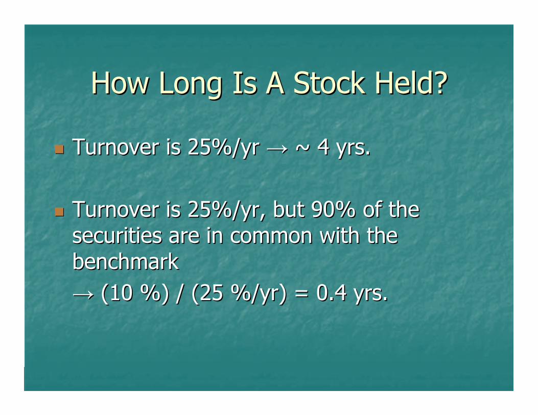
How Long Is A Stock Held?How Long Is A Stock Held?

Turnover is 25%/yr Turnover is 25%/yr →→ ~ 4 yrs.~ 4 yrs.

Turnover is 25%/yr, but 90% of the Turnover is 25%/yr, but 90% of the securities are in common with the securities are in common with the benchmarkbenchmark→→ (10 %) / (25 %/yr) = 0.4 yrs.(10 %) / (25 %/yr) = 0.4 yrs.

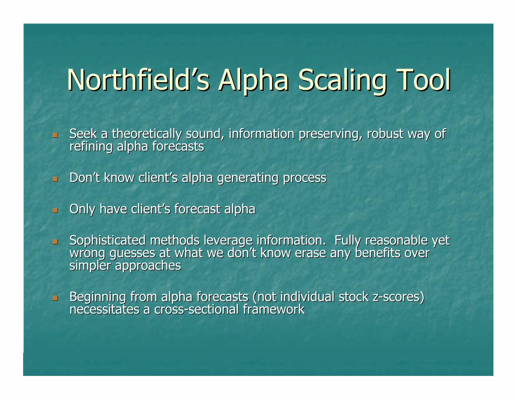
Northfield’s Alpha Scaling ToolNorthfield’s Alpha Scaling Tool

Seek a theoretically sound, information preserving, robust way oSeek a theoretically sound, information preserving, robust way of f refining alpha forecastsrefining alpha forecasts

Don’t know client’s alpha generating processDon’t know client’s alpha generating process

Only have client’s forecast alphaOnly have client’s forecast alpha

Sophisticated methods leverage information. Fully reasonable yeSophisticated methods leverage information. Fully reasonable yet t wrong guesses at what we don’t know erase any benefits over wrong guesses at what we don’t know erase any benefits over simpler approachessimpler approaches

Beginning from alpha forecasts (not individual stock zBeginning from alpha forecasts (not individual stock z--scores) scores) necessitates a crossnecessitates a cross--sectional frameworksectional framework

Preprocessing for Robustness:Preprocessing for Robustness:Rank RescalingRank Rescaling

02468

10121416

2 3 4 5 6 7 8 9

Raw Value

# Se

curit

ies

ρ (raw, reshaped) = .98

0

5

10

15

20

25

-2.5 -1.9 -1.3 -0.6 0.6 1.3 1.9 2.5

Reshaped Value

# Se

curit

ies

Map raw signals by rank onto standard normal Map raw signals by rank onto standard normal e.g. 25e.g. 25thth percentile percentile →→ FF--11(.25)(.25)

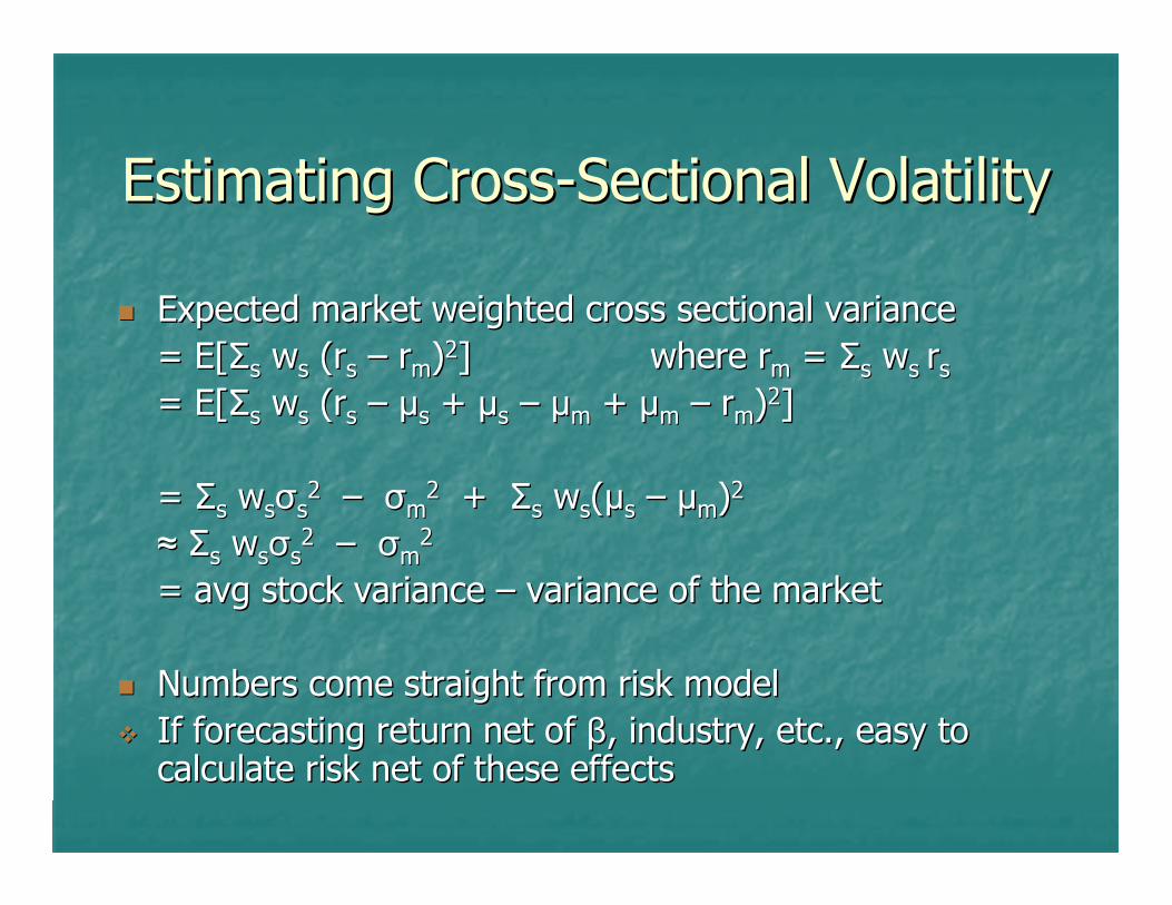
Estimating CrossEstimating Cross--Sectional VolatilitySectional Volatility

Expected market weighted cross sectional varianceExpected market weighted cross sectional variance= E[= E[ΣΣss wwss ((rrss –– rrmm))22]] where where rrmm = = ΣΣss wwss rrss

= E[= E[ΣΣss wwss ((rrss –– µµss + + µµss –– µµmm + + µµmm –– rrmm))22]]

= = ΣΣss wwssσσss22 –– σσmm

22 + + ΣΣss wwss((µµss –– µµmm))22

≈≈ ΣΣss wwssσσss22 –– σσmm

22

= = avgavg stock variance stock variance –– variancevariance of the marketof the market

Numbers come straight from risk modelNumbers come straight from risk modelIf forecasting return net of If forecasting return net of ββ, industry, etc., easy to , industry, etc., easy to calculate risk net of these effectscalculate risk net of these effects

Put The Pieces TogetherPut The Pieces Together

IC IC –– user parameteruser parametercross sectional volatility cross sectional volatility –– from risk modelfrom risk modelscore score –– signal after rank mapping to std Nsignal after rank mapping to std N

Forecast of return above marketForecast of return above market= IC = IC ×× volatility volatility ×× scorescore

SummarySummary

Standard practice alpha scaling methods can be arrived Standard practice alpha scaling methods can be arrived at by following your nose. No hidden magic or at by following your nose. No hidden magic or sophisticationsophistication

Being clear about the inputs and what’s being forecast Being clear about the inputs and what’s being forecast prevents confusionprevents confusion

It is important to be aware of horizon, particularly in It is important to be aware of horizon, particularly in lowlow--turnover portfoliosturnover portfolios

For many practitioners, Northfield’s upcoming alpha For many practitioners, Northfield’s upcoming alpha scaling functionality can make your life easier by doing scaling functionality can make your life easier by doing the work for youthe work for you

ReferencesReferences

GrinoldGrinold, R. “Alpha Is Volatility Times IC Times Score,” , R. “Alpha Is Volatility Times IC Times Score,” Journal of Portfolio ManagementJournal of Portfolio Management, 1994, v20(4,Summer), , 1994, v20(4,Summer), 99--16.16.

Black, F. & Black, F. & LittermanLitterman, R. “Global Portfolio Optimization,” , R. “Global Portfolio Optimization,” Financial Analysts JournalFinancial Analysts Journal, 1992, v48(5,Sept/Oct), 22, 1992, v48(5,Sept/Oct), 22--43.43.

BulsingBulsing, Scowcroft, & , Scowcroft, & SeftonSefton. “Understanding . “Understanding Forecasting: A Unified Framework for Combining Both Forecasting: A Unified Framework for Combining Both Analyst And Strategy Forecasts,” UBS report, 2003.Analyst And Strategy Forecasts,” UBS report, 2003.

AlmgrenAlmgren, R. & , R. & ChrissChriss, N. “Optimal Portfolios from , N. “Optimal Portfolios from Ordering Information”, Ordering Information”, Journal of RiskJournal of Risk, 2006 v9(1,Fall), , 2006 v9(1,Fall), 11--47.47.

Distinguishing Between Being Unlucky and Unskillful

Dan diBartolomeoNorthfield Information Services

June 2007

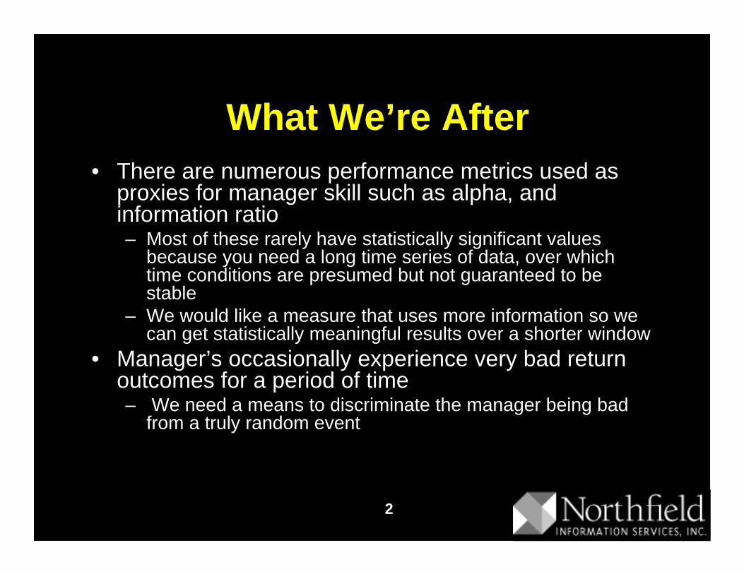
2

What We’re After• There are numerous performance metrics used as

proxies for manager skill such as alpha, and information ratio– Most of these rarely have statistically significant values

because you need a long time series of data, over which time conditions are presumed but not guaranteed to be stable

– We would like a measure that uses more information so we can get statistically meaningful results over a shorter window

• Manager’s occasionally experience very bad return outcomes for a period of time– We need a means to discriminate the manager being bad

from a truly random event

3

What We Probably Don’t Care About

• There is an enormous literature in finance regarding whether asset managers collectively exhibit skill– Obvious implications for concepts of market efficiency– Most of this work is based on the concept of “performance

persistence”: those that perform consistently well must be skillful

– Stewart, Scott D. "Is Consistency Of Performance A Good Measure Of Manager Skill?," Journal of Portfolio Management, 1998, v24(3,Spring), 22-32.

– Brown, Stephen J. and William N. Goetzmann. "Performance Persistence," Journal of Finance, 1995, v50(2), 679-698.

– Elton, Edwin J., Martin J. Gruber and Christopher R. Blake. "The Persistence Of Risk-Adjusted Mutual Fund Performance," Journal of Business, 1996, v69(2,Apr), 133-157.

• But we want to evaluate only one manager

4

Usual Methods• There is lots of literature on using traditional return

performance metrics such as alpha and information ratio as proxies for manager skill:– Kritzman, Mark. "How To Detect Skill In Management

Performance," Journal of Portfolio Management, 1986, v12(2), 16-20.

– Lee, Cheng F. and Shafiqur Rahman. "New Evidence On Timing And Security Selection Skill Of Mutual Fund Managers," Journal of Portfolio Management, 1991, v17(2), 80-83.

– Marcus, Alan J. "The Magellan Fund And Market Efficiency," Journal of Portfolio Management, 1990, v17(1),85-88.

• You need very long time series of return observations to have enough data to get anything statistically significant by which time conditions may change

• Just going to daily data doesn’t help– diBartolomeo, Dan. “Just Because We Can Doesn’t Mean

We Should: Why Daily Attribution is Not Better”, Journal of Performance Measurement, Spring 2003

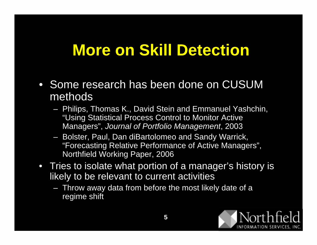
5

More on Skill Detection

• Some research has been done on CUSUM methods – Philips, Thomas K., David Stein and Emmanuel Yashchin,

“Using Statistical Process Control to Monitor Active Managers”, Journal of Portfolio Management, 2003

– Bolster, Paul, Dan diBartolomeo and Sandy Warrick, “Forecasting Relative Performance of Active Managers”, Northfield Working Paper, 2006

• Tries to isolate what portion of a manager’s history is likely to be relevant to current activities– Throw away data from before the most likely date of a

regime shift

6

The Breakdown Problem• Consider a real manager who maintains a below 3%

ex-ante tracking error and has a cumulative return of -6.3% over a one year period– Is this a 2.4 standard deviation event? If so the manager

was very unlucky– Was the risk model wrong? Maybe the risk model was

underestimating the risk so it’s not such a rare event– Expected tracking error averaged 2.74%, realized was

2.80%• Ex-ante tracking error estimate is the expectation of

the standard deviation of the active return, which is measured around the mean– Mean active return was -.54% per month

• Huber, Gerard. “Tracking Error and Active Management”, Northfield Conference Proceedings, 2001, http://www.northinfo.com/documents/164.pdf

7

IR as Skill

• Grinold, Richard C. "The Fundamental Law Of Active Management," Journal of Portfolio Management, 1989, v15(3), 30-37.

• IR = IC * Breadth.5

– IR = alpha / tracking error

IC = correlation of your return forecasts and outcomes

Breadth = number of independent “bets” taken per unit time

• If we know how good we are at forecasting and how many bets we act on, we know how good our performance should be for any given risk level

8

The Fundamental Law Makes Big Assumptions

• There are no constraints at all on portfolio construction– Positions can be long or short and of any size

• We measure only “independent” bets– Buying 20 different stocks for 20 different reasons is 20

different bets– Buying 20 stocks because they all have a low PE is one bet,

not 20!• Transaction costs are zero, so bets in one time

period are independent of bets in other periods– This is the property that casinos depend on. Once we have

the odds in our favor, we want to make lots of bets• Research resources are limitless so our forecasting

effectiveness (IC) is constant as we increase the number of eligible assets

9

Enter the Transfer Coefficient

• Clarke, Roger, Harindra de Silva and Steven Thorley. "Portfolio Constraints And The Fundamental Law Of Active Management," Financial Analyst Journal, 2002, v58(5,Sep/Oct), 48-66.

• IR = IC * TC * Breadth.5

– IR = alpha / tracking error

IC = correlation of your return forecasts and outcomes

TC = the efficiency of your portfolio construction (TC < 1)

Breadth = number of independent “bets” taken per unit time

10

What Drives the Transfer Coefficient?

• Imagine a manager with a diverse team of analysts that are great at forecasting monthly stock returns on a large universe of stocks, but whose portfolio is allowed to have only 1% per year turnover– Good monthly forecasts, diverse reasons and a large

universe imply high IC and high breadth– But if we can never act on the forecasts because of the

turnover constraint TC can be zero or even negative• If we can’t short a stock that we correctly believe is

going down, or take a big position in a stock that we correctly believe is going up, TC declines– The more binding constraints we have on our portfolio

construction, the more return we fail to capture when our forecasts are good

– For bad forecasters, a low TC is good. You hurt yourself less when you constrain your level of activity

11

Limitations of IR• Managers often talk about IR, but it really doesn’t

correspond to investor utility except in extreme cases– Consider a manager with an alpha of 1 basis point and a

tracking error of zero– IR is infinite but value added for the investor is very, very

small – deGroot, Sebastien and Auke Plantinga, “Risk Adjusted

Performance Measures and Implied Risk Attitudes”, Journal of Performance Measurement, Winter 2001/2002

• The statistical significance of a ratio is hard to calculate– Jobson, J. D. and Bob M. Korkie. "Performance Hypothesis

Testing With The Sharpe And Treynor Measures," Journal of Finance, 1981, v36(4), 889-908.

12

Our Solution is to Incorporate Cross-Sectional Information

• Successful active management involves forecasting what returns different assets will earn in the future, and forming portfolios that will efficiently use the valid information contained in the forecast– We usually have a large universe of assets to work with, so

we get statistical significance quickly– In mathematical terms, this means that the position sizes

within our portfolios balance the marginal returns, risks and costs

– If we know how good we are at forecasting future asset returns, we can forecast how well our portfolios should perform if they are efficiently constructed. If we do less well than we should, our portfolio construction is at fault

13

A Quant Way to Think About It• Every portfolio manager must believe that the

portfolio they hold is optimal for their investors– If they didn’t they would hold a different portfolio

• If we describe investor goals as maximizing risk adjusted returns, we know that the marginal risks associated with every active position must be exactly offset by the expected active returns– Guaranteed by the Kuhn Tucker conditions for finding the

maximum of a polynomial function– For every portfolio, there exists a set of alpha (active return)

expectations that would make the portfolio optimal. We call these the implied alphas

– Sharpe, William F. "Imputing Expected Security Returns From Portfolio Composition," Journal of Financial and Quantitative Analysis, 1974, v9(3), 462-472.

14

The Effective Information Coefficient

• We define the EIC as the skill measure• EIC is the pooled average rank correlation of the

implied alphas and the realized returns at the security level– If our forecasting skill is good (high IC) and our portfolio

construction skill is good (high TC) then EIC will be high– If either IC or TC is low, EIC will be low

• As this measurement involves every active position during each time period, the sample is large and statistical significance is obtained quickly

15

Using EIC to Dissect Performance

• If we have EIC values for a given period (e.g. month), we can estimate the expected magnitude of alpha

• The expected alpha is just the EIC times the cross-sectional dispersion of the asset returns

• So we can look at returns as:

Pt – Bt = EICt * Dt + εt

Pt = portfolio return during period t Bt = benchmark return during period tEICt = skill for period t Dt = cross sectional dispersion of asset returnsεt = residual returns due to luck

• You can now look at the time series standard deviation of the εt to see if the risk model is predicting risk accurately

16

An Alternative View• Active managers can add value in two ways:

– Being right more often than they are wrong about which securities will outperform the market. Sort of like a batting average in baseball

– Getting bigger magnitude returns on gainers than on losers. You can have a batting average below 50% and still make money if you hit a decent number of “home runs”

• Peter Lynch used to refer to “ten baggers”– Stocks that go up ten fold in value while you hold them– Just a couple can have a huge effect on portfolio returns

• Batting average concept first formalized in:– Sorensen, Eric H., Keith L. Miller and Vele Samak.

"Allocating Between Active And Passive Management," Financial Analyst Journal, 1998, v54(5,Sep/Oct), 18-31.

17

Attribution to Batting Average and Active Return Skew

• A formalization was proposed by hedge fund manager Andrei Pokrovsky (formerly Northfield staff) in 2006

• We can easily measure batting average– It is the percentage of cases in which active returns and

active weights are of the same sign– High numbers are good

• Take the vector product of active weights and active returns. Measure the skew statistic of the distribution– Positive skew in active returns is a measure of portfolio

construction efficiency

18

Style Dependency of Batting Average and Active Skew

• Value managers will tend to have high batting average and low skew

• Growth/momentum managers will tend to have lower batting average but higher skew

• Trend following behavior creates the skew– Wilcox, Jarrod W. "Better Risk Management," Journal of

Portfolio Management, 2000, v26(4,Summer), 53-64.– diBartolomeo (2003)

http://www.northinfo.com/documents/132.pdf– Bondarenko, Oleg. “The Market Price of Variance Risk and

the Performance of Hedge Funds”, University of Illinois-Chicago Working Paper, 2004.

19

Conclusions

• Its often difficult to assess whether a period of extraordinary performance (good or bad) is the result of luck or skill

• We propose the Effective Information Coefficient as a measure of skill– It is estimated both over time and across assets so sample

sizes get large quickly– It incorporates both key aspects of investment skill,

forecasting returns and forming efficient portfolios• We present an alternative representation of skill as

“batting average” and “payoff skew”