northwestern university - european central bank · northwestern university 9th ecb workshop on...
TRANSCRIPT

Priorsforthelongrun
Giannone,Lenza,Prim iceri Priors for the long run
Domenico GiannoneNewYorkFed
MicheleLenzaEuropeanCentralBank
GiorgioPrimiceriNorthwesternUniversity
9th ECB Workshop on Forecasting TechniquesJune3,2016

Giannone,Lenza,Prim iceri Priors for the long run
Whatwedo
n ProposeaclassofpriordistributionsforVARsthatdisciplinethelong-runimplicationsofthemodel
Priorsforthelongrun

Giannone,Lenza,Prim iceri Priors for the long run
Whatwedo
n ProposeaclassofpriordistributionsforVARsthatdisciplinethelong-runimplicationsofthemodel
Priorsforthelongrun
n PropertiesØ BasedonmacroeconomictheoryØ Conjugateà Easy toimplement andcombinewithexistingpriors
n Performwell inapplicationsØ Good(long-run)forecastingperformance

Giannone,Lenza,Prim iceri Priors for the long run
Outline
n Aspecificpathologyof(flat-prior)VARsØ Toomuchexplanatorypowerofinitialconditionsanddeterministic trendsØ Sims(1996and2000)
n PriorsforthelongrunØ IntuitionØ Specificationandimplementation
n Alternativeinterpretationsandrelationwiththeliterature
n Application:macroeconomicforecasting

Giannone,Lenza,Prim iceri Priors for the long run
Simpleexample
n AR(1):
€
yt = c + ρyt−1 +ε t

Giannone,Lenza,Prim iceri Priors for the long run
Simpleexample
n AR(1):
n Iteratebackwards:
€
yt = c + ρyt−1 +ε t
€
yt = ρ t y0 + ρ jcj=0
t−1∑ + ρ jε t− jj=0
t−1∑

Giannone,Lenza,Prim iceri Priors for the long run
Simpleexample
n AR(1):
n Iteratebackwards:
➠ModelseparatesobservedvariationofthedataintoØ DC:deterministic component,predictablefromdataattime0Ø SC:unpredictable/stochastic component
€
yt = c + ρyt−1 +ε t
€
yt = ρ t y0 + ρ jcj=0
t−1∑ + ρ jε t− jj=0
t−1∑
SCDC

Giannone,Lenza,Prim iceri Priors for the long run
Simpleexample
n AR(1):
n Iteratebackwards:
➠ModelseparatesobservedvariationofthedataintoØ DC:deterministic component,predictablefromdataattime0Ø SC:unpredictable/stochastic component
n Ifρ =1,DCisasimplelineartrend:
€
yt = c + ρyt−1 +ε t
€
yt = ρ t y0 + ρ jcj=0
t−1∑ + ρ jε t− jj=0
t−1∑
€
DC = y0 + c⋅ t
SCDC

Giannone,Lenza,Prim iceri Priors for the long run
Simpleexample
n AR(1):
n Iteratebackwards:
➠ModelseparatesobservedvariationofthedataintoØ DC:deterministic component,predictablefromdataattime0Ø SC:unpredictable/stochastic component
n Ifρ =1,DCisasimplelineartrend:
n Otherwisemorecomplex:
€
yt = c + ρyt−1 +ε t
€
yt = ρ t y0 + ρ jcj=0
t−1∑ + ρ jε t− jj=0
t−1∑
€
DC = y0 + c⋅ t
€
DC =c
1− ρ+ ρ t y0 −
c1− ρ
$
% &
'
( )
SCDC

Giannone,Lenza,Prim iceri Priors for the long run
Pathologyof(flat-prior)VARs(Sims,1996and2000)
n OLS/MLEhasatendencyto“use”thecomplexityofdeterministiccomponentstofitthelowfrequencyvariationinthedata
n Possiblebecauseinferenceistypicallyconditionalony0Ø Nopenalizationforparameterestimates ofimplyingsteadystates ortrendsfar
awayfrominitialconditions

Giannone,Lenza,Prim iceri Priors for the long run
DeterministiccomponentsinVARs
n ProblemmoreseverewithVARsØ implieddeterministic component ismuchmorecomplexthaninAR(1)case

Giannone,Lenza,Prim iceri Priors for the long run
DeterministiccomponentsinVARs
n ProblemmoreseverewithVARsØ implieddeterministic component ismuchmorecomplexthaninAR(1)case
n Example:7-variableVAR(5)withquarterlydataonØ GDPØ ConsumptionØ InvestmentØ RealWagesØ HoursØ InflationØ Federalfundsrate
n Sample:1955:I– 1994:IV
n FlatorMinnesotaprior

Giannone,Lenza,Prim iceri Priors for the long run
“Over-fitting”ofdeterministiccomponentsinVARs
1960 1980 2000
5.55.65.75.85.9
66.16.26.36.4
GDP
1960 1980 20003.9
44.14.24.34.44.54.64.7
Investment
1960 1980 2000
-0.65
-0.6
-0.55
-0.5
Hours
1960 1980 2000
-1.7-1.65
-1.6-1.55
-1.5-1.45
-1.4-1.35
-1.3-1.25
Investment-to-GDP ratio
1960 1980 2000-0.015
-0.01-0.005
00.005
0.010.015
0.020.025
Inflation
1960 1980 2000
-0.01
0
0.01
0.02
0.03
0.04
Interest rate
Data Flat MN PLR

Giannone,Lenza,Prim iceri Priors for the long run
Pathologyof(flat-prior)VARs(Sims,1996and2000)
n OLS/MLEhasatendencyto“use”thecomplexityofdeterministiccomponentstofitthelowfrequencyvariationinthedata
n Possiblebecauseinferenceistypicallyconditionalony0Ø Nopenalizationforparameterestimates ofimplyingsteadystates ortrendsfar
awayfrominitialconditions
➠Flat-priorVARsattributean(implausibly) largeshareofthelowfrequencyvariationinthedatatodeterministiccomponents
n Needapriorthatdownplaysexcessiveexplanatorypowerofinitialconditionsanddeterministiccomponent
n Onesolution:centerprioron“non-stationarity”

Giannone,Lenza,Prim iceri Priors for the long run
Outline
n Aspecificpathologyof(flat-prior)VARsØ Toomuchexplanatorypowerofinitialconditionsanddeterministic trendsØ Sims(1996and2000)
n PriorsforthelongrunØ IntuitionØ Specificationandimplementation
n Alternativeinterpretationsandrelationwiththeliterature
n Application:macroeconomicforecasting

Giannone,Lenza,Prim iceri Priors for the long run
Priorforthelongrun
€
VAR(1) : yt = c + Byt−1 +ε t , ε t ~ N 0,Σ( )

Giannone,Lenza,Prim iceri Priors for the long run
Priorforthelongrun
n RewritetheVARintermsoflevelsanddifferences:
€
VAR(1) : yt = c + Byt−1 +ε t , ε t ~ N 0,Σ( )
€
Δyt = c +Πyt−1 +ε tΠ = B − I

Giannone,Lenza,Prim iceri Priors for the long run
Priorforthelongrun
n RewritetheVARintermsoflevelsanddifferences:
n Priorforthelongrun prioroncenteredat0
€
VAR(1) : yt = c + Byt−1 +ε t , ε t ~ N 0,Σ( )
€
Δyt = c +Πyt−1 +ε tΠ = B − I
€
Π

Giannone,Lenza,Prim iceri Priors for the long run
Priorforthelongrun
n RewritetheVARintermsoflevelsanddifferences:
n Priorforthelongrun prioroncenteredat0
n Standardapproach(DLS,SZ,andmanyfollowers)Ø Pushcoefficientstowardsallvariablesbeingindependentrandomwalks
€
VAR(1) : yt = c + Byt−1 +ε t , ε t ~ N 0,Σ( )
€
Δyt = c +Πyt−1 +ε tΠ = B − I
€
Π

Giannone,Lenza,Prim iceri Priors for the long run
Priorforthelongrun
n Rewriteas
€
Δyt = c +Πyt−1 +ε t
€
Δyt = c +Π H −1
Λ! " # Hyt−1
˜ y t−1
! " # +ε t

Giannone,Lenza,Prim iceri Priors for the long run
Priorforthelongrun
n Rewriteas
n ChooseH andputprioronΛ conditionalonH
€
Δyt = c +Πyt−1 +ε t
€
Δyt = c +Π H −1
Λ! " # Hyt−1
˜ y t−1
! " # +ε t

Giannone,Lenza,Prim iceri Priors for the long run
Priorforthelongrun
n Rewriteas
n ChooseH andputprioronΛ conditionalonH
n Economictheorysuggeststhatsomelinearcombinationsofy areless(more)likelytoexhibitlong-runtrends
€
Δyt = c +Πyt−1 +ε t
€
Δyt = c +Π H −1
Λ! " # Hyt−1
˜ y t−1
! " # +ε t

Giannone,Lenza,Prim iceri Priors for the long run
Priorforthelongrun
n Rewriteas
n ChooseH andputprioronΛ conditionalonH
n Economictheorysuggeststhatsomelinearcombinationsofy areless(more)likelytoexhibitlong-runtrends
n Loadingsassociatedwiththesecombinationsareless(more)likelytobe0
€
Δyt = c +Πyt−1 +ε t
€
Δyt = c +Π H −1
Λ! " # Hyt−1
˜ y t−1
! " # +ε t

Giannone,Lenza,Prim iceri Priors for the long run
Example:3-variableVARofKPSW
OutputConsumptionInvestment
€
Δyt = c +Π H −1
Λ! " # Hyt−1
˜ y t−1
! " # +ε t
€
1 1 1−1 1 0−1 0 1
#
$
% % %
&
'
( ( (

Giannone,Lenza,Prim iceri Priors for the long run
Example:3-variableVARofKPSW
OutputConsumptionInvestment
€
ΔxtΔctΔit
#
$
% % %
&
'
( ( (
= c +
Λ11 Λ12 Λ13
Λ21 Λ22 Λ23
Λ31 Λ32 Λ33
#
$
% % %
&
'
( ( (
xt−1 + ct−1 + it−1
ct−1 − xt−1
it−1 − xt−1
#
$
% % %
&
'
( ( ( +ε t
€
Δyt = c +Π H −1
Λ! " # Hyt−1
˜ y t−1
! " # +ε t
Possibly stationary linear combinations
€
1 1 1−1 1 0−1 0 1
#
$
% % %
&
'
( ( (

Giannone,Lenza,Prim iceri Priors for the long run
Example:3-variableVARofKPSW
OutputConsumptionInvestment
€
ΔxtΔctΔit
#
$
% % %
&
'
( ( (
= c +
Λ11 Λ12 Λ13
Λ21 Λ22 Λ23
Λ31 Λ32 Λ33
#
$
% % %
&
'
( ( (
xt−1 + ct−1 + it−1
ct−1 − xt−1
it−1 − xt−1
#
$
% % %
&
'
( ( ( +ε t
€
Δyt = c +Π H −1
Λ! " # Hyt−1
˜ y t−1
! " # +ε t
Common trend
Possibly stationary linear combinations
€
1 1 1−1 1 0−1 0 1
#
$
% % %
&
'
( ( (
Giannone,Lenza,Prim iceri Priors for the long run
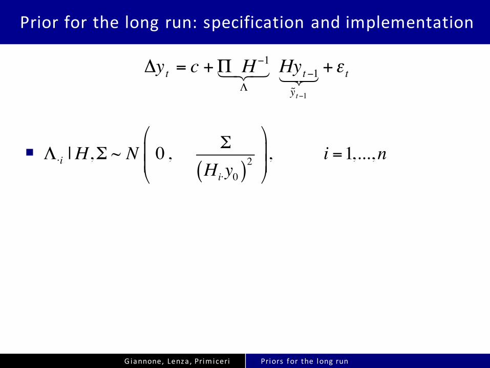
Priorforthelongrun:specificationandimplementation
n
€
Δyt = c +Π H −1
Λ! " # Hyt−1
˜ y t−1
! " # +ε t
Λ⋅i |H,Σ ~ N 0 , φi2 Σ
Hi⋅y0( )2 $
%&&
'
()), i =1,...,n

Giannone,Lenza,Prim iceri Priors for the long run
Priorforthelongrun:specificationandimplementation
n
€
Δyt = c +Π H −1
Λ! " # Hyt−1
˜ y t−1
! " # +ε t
Λ⋅i |H,Σ ~ N 0 , φi2 Σ
Hi⋅y0( )2 $
%&&
'
()), i =1,...,n

Giannone,Lenza,Prim iceri Priors for the long run
Priorforthelongrun:specificationandimplementation
n
n ConjugateØ Canimplement itwithTheilmixedestimation intheVARinlevels
€
Δyt = c +Π H −1
Λ! " # Hyt−1
˜ y t−1
! " # +ε t
Λ⋅i |H,Σ ~ N 0 , φi2 Σ
Hi⋅y0( )2 $
%&&
'
()), i =1,...,n

Giannone,Lenza,Prim iceri Priors for the long run
Priorforthelongrun:specificationandimplementation
n
n ConjugateØ Canimplement itwithTheilmixedestimation intheVARinlevelsØ Canbeeasilycombinedwithexistingpriors
€
Δyt = c +Π H −1
Λ! " # Hyt−1
˜ y t−1
! " # +ε t
Λ⋅i |H,Σ ~ N 0 , φi2 Σ
Hi⋅y0( )2 $
%&&
'
()), i =1,...,n

Giannone,Lenza,Prim iceri Priors for the long run
Priorforthelongrun:specificationandimplementation
n
n ConjugateØ Canimplement itwithTheilmixedestimation intheVARinlevelsØ CanbeeasilycombinedwithexistingpriorsØ CancomputetheMLinclosedform
n Usefulforhierarchicalmodelingandsettingofhyperparameters ϕ (GLP,2013)
€
Δyt = c +Π H −1
Λ! " # Hyt−1
˜ y t−1
! " # +ε t
Λ⋅i |H,Σ ~ N 0 , φi2 Σ
Hi⋅y0( )2 $
%&&
'
()), i =1,...,n

Giannone,Lenza,Prim iceri Priors for the long run
Empiricalresults
n Deterministiccomponentin7-variableVAR
n ForecastingØ 3-variableVARØ 5-variableVARØ 7-variableVAR

Giannone,Lenza,Prim iceri Priors for the long run
Empiricalresults
n Deterministiccomponentin7-variableVAR

Giannone,Lenza,Prim iceri Priors for the long run
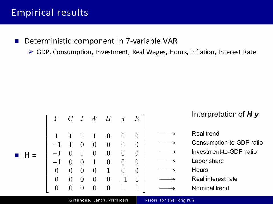
Empiricalresults
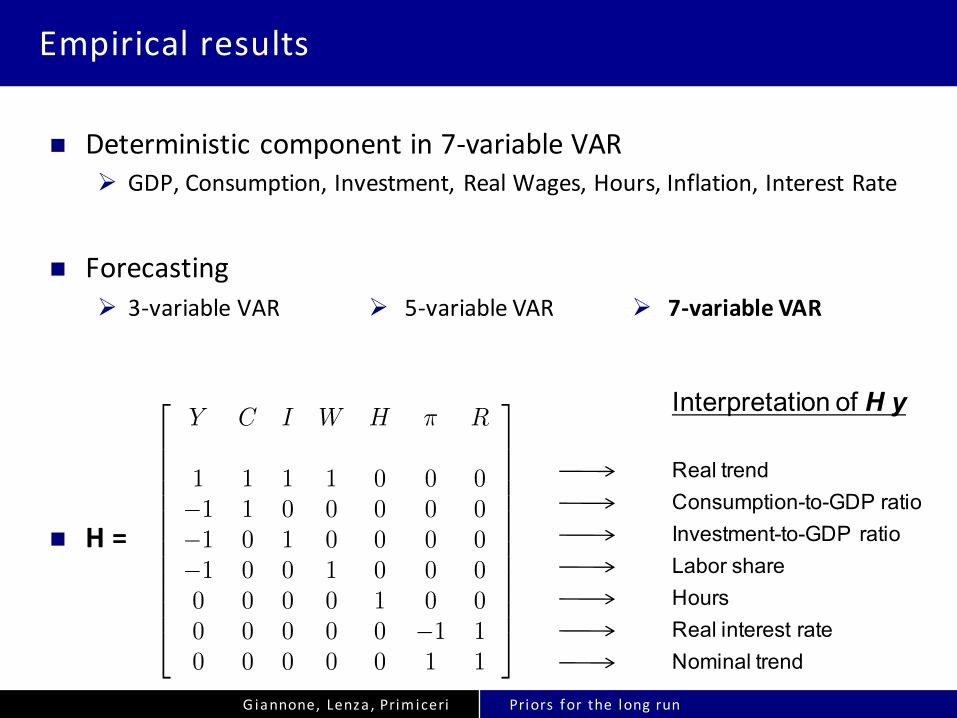
n Deterministiccomponentin7-variableVARØ GDP,Consumption,Investment,RealWages,Hours,Inflation,InterestRate
Giannone,Lenza,Prim iceri Priors for the long run
Empiricalresults
n Deterministiccomponentin7-variableVARØ GDP,Consumption,Investment,RealWages,Hours,Inflation,InterestRate
n H=
Real trendConsumption-to-GDP ratioInvestment-to-GDP ratioLabor shareHoursReal interest rateNominal trend
Interpretation of H y2
6666666666664
Y C I W H ⇡ R
1 1 1 1 0 0 0�1 1 0 0 0 0 0�1 0 1 0 0 0 0�1 0 0 1 0 0 00 0 0 0 1 0 00 0 0 0 0 �1 10 0 0 0 0 1 1
3
7777777777775
1

Giannone,Lenza,Prim iceri Priors for the long run
Empiricalresults
n Deterministiccomponentin7-variableVARØ GDP,Consumption,Investment,RealWages,Hours,Inflation,InterestRate
n ForecastingØ 3-variableVAR
n H=
Real trendConsumption-to-GDP ratioInvestment-to-GDP ratioLabor shareHoursReal interest rateNominal trend
Interpretation of H y2
6666666666664
Y C I W H ⇡ R
1 1 1 1 0 0 0�1 1 0 0 0 0 0�1 0 1 0 0 0 0�1 0 0 1 0 0 00 0 0 0 1 0 00 0 0 0 0 �1 10 0 0 0 0 1 1
3
7777777777775
1
Ø 5-variableVAR Ø 7-variableVAR

Giannone,Lenza,Prim iceri Priors for the long run
DeterministiccomponentsinVARs
1960 1980 2000
5.55.65.75.85.9
66.16.26.36.4
GDP
1960 1980 20003.9
44.14.24.34.44.54.64.7
Investment
1960 1980 2000
-0.65
-0.6
-0.55
-0.5
Hours
1960 1980 2000
-1.7-1.65
-1.6-1.55
-1.5-1.45
-1.4-1.35
-1.3-1.25
Investment-to-GDP ratio
1960 1980 2000-0.015
-0.01-0.005
00.005
0.010.015
0.020.025
Inflation
1960 1980 2000
-0.01
0
0.01
0.02
0.03
0.04
Interest rate
Data Flat MN PLR

Giannone,Lenza,Prim iceri Priors for the long run
DeterministiccomponentsinVARswithPriorfortheLongRun
1960 1980 2000
5.5
6
6.5GDP
1960 1980 2000
4
4.2
4.4
4.6
4.8
5Investment
1960 1980 2000
-0.65
-0.6
-0.55
-0.5
Hours
1960 1980 2000
-1.7-1.65
-1.6-1.55
-1.5-1.45
-1.4-1.35
-1.3-1.25
Investment-to-GDP ratio
1960 1980 2000-0.015
-0.01-0.005
00.005
0.010.015
0.020.025
Inflation
1960 1980 2000
-0.01
0
0.01
0.02
0.03
0.04
Interest rate
Data Flat MN PLR

Giannone,Lenza,Prim iceri Priors for the long run
Forecastingresultswith3-,5- and7-variableVARs
n Recursiveestimationstartsin1955:I
n Forecast-evaluationsample:1985:I– 2013:I

Giannone,Lenza,Prim iceri Priors for the long run
3-variableVAR:MSFE(1985-2013)
0 10 20 30 40
MSF
E
0
0.002
0.004
0.006
0.008
0.01Y
Quarters ahead0 10 20 30 40
MSF
E
0
0.02
0.04
0.06
0.08
0.1
0.12
0.14Y + C + I
0 10 20 30 40 0
0.002
0.004
0.006
0.008
0.01
0.012
0.014C
Quarters ahead0 10 20 30 40
0
0.0002
0.0004
0.0006
0.0008
0.001
0.0012C - Y
0 10 20 30 40 0
0.01
0.02
0.03
0.04
0.05
0
0.01
0.02
0.03I
Quarters ahead0 10 20 30 40
0
0.005
0.01
0.015
0.02
0.025
0.03I - Y
MN SZ Naive PLR

Giannone,Lenza,Prim iceri Priors for the long run
3-variableVAR:MSFE(1985-2013)
0 10 20 30 40
MSF
E
0
0.002
0.004
0.006
0.008
0.01Y
Quarters ahead0 10 20 30 40
MSF
E
0
0.02
0.04
0.06
0.08
0.1
0.12
0.14Y + C + I
0 10 20 30 40 0
0.002
0.004
0.006
0.008
0.01
0.012
0.014C
Quarters ahead0 10 20 30 40
0
0.0002
0.0004
0.0006
0.0008
0.001
0.0012C - Y
0 10 20 30 40 0
0.01
0.02
0.03
0.04
0.05I
Quarters ahead0 10 20 30 40
0
0.005
0.01
0.015
0.02
0.025
0.03I - Y
MN SZ Naive PLR

Giannone,Lenza,Prim iceri Priors for the long run
Consumption- andInvestment-to-GDPratios
1960 1970 1980 1990 2000 2010-0.65
-0.6
-0.55
-0.5
C - Y
1960 1970 1980 1990 2000 2010-1.7
-1.6
-1.5
-1.4
-1.3
I - Y
Actual Naive PLR

Giannone,Lenza,Prim iceri Priors for the long run
Forecasts(5yearsahead)
1960 1970 1980 1990 2000 2010-0.65
-0.6
-0.55
-0.5
C - Y
1960 1970 1980 1990 2000 2010-1.7
-1.6
-1.5
-1.4
-1.3
I - Y
Actual Naive PLR

Giannone,Lenza,Prim iceri Priors for the long run
Forecasts(5yearsahead)
1960 1970 1980 1990 2000 2010-0.65
-0.6
-0.55
-0.5
C - Y
1960 1970 1980 1990 2000 2010-1.7
-1.6
-1.5
-1.4
-1.3
I - Y
Actual Naive PLR

Giannone,Lenza,Prim iceri Priors for the long run
5-variableVAR:MSFE(1985-2013)
0 10 20 30 40
MSF
E
0
0.001
0.002
0.003
0.004
0.005
0.006
0.007
0.008Y
0 10 20 30 40M
SFE
0
0.002
0.004
0.006
0.008
0.01
0.012C
0 10 20 30 40
MSF
E
0
0.01
0.02
0.03
0.04
0.05
0.06
0.07
0.08I
Quarters Ahead0 10 20 30 40
MSF
E
0
0.001
0.002
0.003
0.004
0.005
0.006
0.007H
Quarters Ahead0 10 20 30 40
MSF
E
0
0.002
0.004
0.006
0.008
0.01
0.012W
MNSZNaivePLR

Giannone,Lenza,Prim iceri Priors for the long run
7-variableVAR:MSFE(1985-2013)
0 20 40
MSF
E
00.0010.0020.0030.0040.0050.0060.0070.0080.009 0.01
Y
0 20 40
MSF
E
0
0.002
0.004
0.006
0.008
0.01
0.012
0.014C
0 20 40
MSF
E
0
0.01
0.02
0.03
0.04
0.05
0.06
0.07
0.08I
0 20 40
MSF
E
0
0.001
0.002
0.003
0.004
0.005
0.006
0.007
0.008
0.009H
Quarters Ahead0 20 40
MSF
E
00.0020.0040.0060.008 0.01
0.0120.0140.0160.018 0.02
W
Quarters Ahead0 20 40
MSF
E
0
2e-05
4e-05
6e-05
8e-05
0.0001
0.00012:
Quarters Ahead0 20 40
MSF
E
0
5e-05
0.0001
0.00015
0.0002
0.00025
0.0003R
MNSZNaivePLR
𝝅
Giannone,Lenza,Prim iceri Priors for the long run
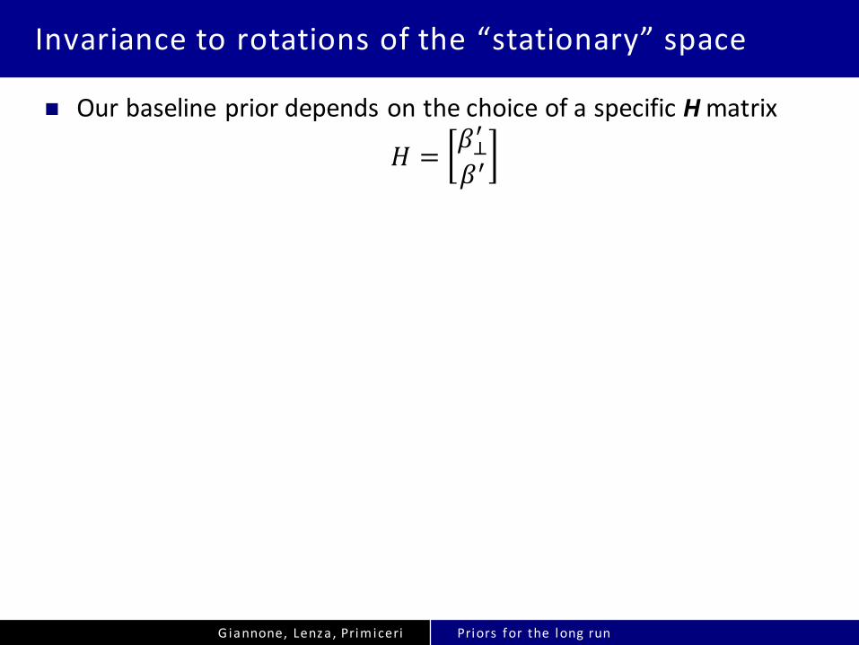
Invariancetorotationsofthe“stationary”space
n OurbaselinepriordependsonthechoiceofaspecificHmatrix
𝐻 = 𝛽%&
𝛽&

Giannone,Lenza,Prim iceri Priors for the long run
Invariancetorotationsofthe“stationary”space
n OurbaselinepriordependsonthechoiceofaspecificHmatrix
𝐻 = 𝛽%&
𝛽&
n Economictheoryisuseful,butnotsufficienttouniquelypindownHØ Macromodelsaretypically informativeabout𝜷%andsp(𝜷)

Giannone,Lenza,Prim iceri Priors for the long run
Invariancetorotationsofthe“stationary”space
n OurbaselinepriordependsonthechoiceofaspecificHmatrix
𝐻 = 𝛽%&
𝛽&
n Economictheoryisuseful,butnotsufficienttouniquelypindownHØ Macromodelsaretypically informativeabout𝜷%andsp(𝜷)
➠ ExtensionofourPLRthatisinvarianttorotationsof𝜷
BaselinePLR: Λ*+ * 𝐻+*𝑦-. |𝐻, Σ~𝑁 0,𝜙+6Σ , 𝑖 = 1, … ,𝑛
InvariantPLR: ;Λ*+ * 𝐻+*𝑦-. |𝐻, Σ~𝑁 0,𝜙+6Σ , 𝑖 = 1, … ,𝑛 − 𝑟
∑ Λ*+ * 𝐻+*𝑦-. |𝐻, Σ~𝑁 0,𝜙?@ABC6 Σ?+D?@ABC

Giannone,Lenza,Prim iceri Priors for the long run
7-variableVAR:Forecasting resultswith“invariant”PLR
0 20 40
MS
FE
0
0.002
0.004
0.006
0.008
0.01Y
0 20 40M
SFE
0
0.002
0.004
0.006
0.008
0.01C
0 20 40
MS
FE
0
0.01
0.02
0.03
0.04
0.05I
0 20 40
MS
FE
0
0.002
0.004
0.006
0.008H
0 20 40
MS
FE
0
2e-05
4e-05
6e-05
8e-05
0.0001π
0 20 40M
SFE
0
2e-05
4e-05
6e-05
8e-05
0.0001
0.00012R
Quarters Ahead0 20 40
MS
FE
0
0.0005
0.001
0.0015
0.002
0.0025
0.003C - Y
Quarters Ahead0 20 40
MS
FE
0
0.005
0.01
0.015
0.02
0.025I - Y
Quarters Ahead0 20 40
MS
FE
0
0.0005
0.001
0.0015
0.002W - Y
PLR baseline PLR invariant PLR invariant (except C-Y)

Giannone,Lenza,Prim iceri Priors for the long run
Hy inthedata
1940 1960 1980 2000 2020-0.7
-0.65
-0.6
-0.55
-0.5
-0.45C-Y
1940 1960 1980 2000 2020-1.8
-1.7
-1.6
-1.5
-1.4
-1.3
-1.2I-Y
1940 1960 1980 2000 2020-0.72-0.7-0.68-0.66-0.64-0.62-0.6-0.58-0.56-0.54-0.52
H
1940 1960 1980 2000 2020-0.62
-0.6
-0.58
-0.56
-0.54
-0.52
-0.5W-Y
1940 1960 1980 2000 2020-0.01
0
0.01
0.02
0.03
0.04
0.05
0.06
0.07R+:
1940 1960 1980 2000 2020-0.01
-0.005
0
0.005
0.01
0.015
0.02
0.025
0.03R-:𝝅 𝝅

Giannone,Lenza,Prim iceri Priors for the long run
7-variableVAR:Forecasting resultswith“invariant”PLR
0 20 40
MS
FE
0
0.002
0.004
0.006
0.008
0.01Y
0 20 40M
SFE
0
0.002
0.004
0.006
0.008
0.01C
0 20 40
MS
FE
0
0.01
0.02
0.03
0.04
0.05I
0 20 40
MS
FE
0
0.002
0.004
0.006
0.008H
0 20 40
MS
FE
0
2e-05
4e-05
6e-05
8e-05
0.0001π
0 20 40M
SFE
0
2e-05
4e-05
6e-05
8e-05
0.0001
0.00012R
Quarters Ahead0 20 40
MS
FE
0
0.0005
0.001
0.0015
0.002
0.0025
0.003C - Y
Quarters Ahead0 20 40
MS
FE
0
0.005
0.01
0.015
0.02
0.025I - Y
Quarters Ahead0 20 40
MS
FE
0
0.0005
0.001
0.0015
0.002W - Y
PLR baseline PLR invariant PLR invariant (except C-Y)

Giannone,Lenza,Prim iceri Priors for the long run
Strengthsandweaknesses
n StrengthsØ Imposesdiscipline onlong-runbehaviorofthemodelØ BasedonrobustlessonsoftheoreticalmacromodelsØ Performswellinforecasting(especially atlongerhorizons)Ø Veryeasytoimplement

Giannone,Lenza,Prim iceri Priors for the long run
Strengthsandweaknesses
n StrengthsØ Imposesdiscipline onlong-runbehaviorofthemodelØ BasedonrobustlessonsoftheoreticalmacromodelsØ Performswellinforecasting(especially atlongerhorizons)Ø Veryeasytoimplement
n “Weak”pointsØ Non-automaticprocedureà needtothinkaboutitØ Mightprovedifficulttosetupinlarge-scalemodelsà mightrequiretoo
muchthinking

Giannone,Lenza,Prim iceri Priors for the long run
Connectionsandextremecases
n Rewriteas
€
Δyt = c +Π H −1
Λ! " # Hyt−1
˜ y t−1
! " # +ε t
Δyt = c+ Λ1 Λ2[ ] β⊥ 'β '$
%&
'
()yt−1 +εt

Giannone,Lenza,Prim iceri Priors for the long run
Connectionsandextremecases
n Rewriteas
€
Δyt = c +Π H −1
Λ! " # Hyt−1
˜ y t−1
! " # +ε t
Δyt = c+ Λ1 Λ2[ ] β⊥ 'β '$
%&
'
()yt−1 +εt
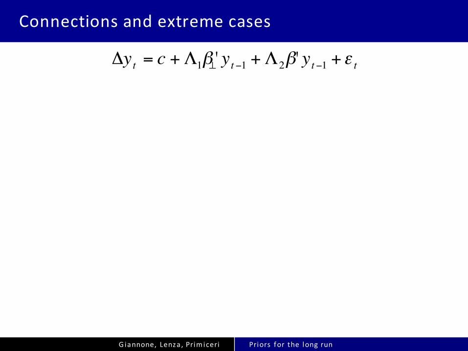
Δyt = c+Λ1β⊥ ' yt−1 +Λ2β ' yt−1 +εt
Giannone,Lenza,Prim iceri Priors for the long run
Connectionsandextremecases
€
Δyt = c +Λ1β⊥' yt−1 +Λ2β' yt−1 +ε t

Giannone,Lenza,Prim iceri Priors for the long run
Connectionsandextremecases
n ErrorCorrectionModel:dogmaticprioronΛ1=0
€
Δyt = c +Λ1β⊥' yt−1 +Λ2β' yt−1 +ε t

Giannone,Lenza,Prim iceri Priors for the long run
Connectionsandextremecases
n ErrorCorrectionModel:dogmaticprioronΛ1=0
€
Δyt = c +Λ1β⊥' yt−1 +Λ2β' yt−1 +ε t
Ø KPSW,CEEn fixβ basedontheoryn flatprioronΛ2

Giannone,Lenza,Prim iceri Priors for the long run
Connectionsandextremecases
n ErrorCorrectionModel:dogmaticprioronΛ1=0
€
Δyt = c +Λ1β⊥' yt−1 +Λ2β' yt−1 +ε t
Ø KPSW,CEEn fixβ basedontheoryn flatprioronΛ2
Ø Cointegrationn estimateβn flatprioronΛ2
n EG(1987)

Giannone,Lenza,Prim iceri Priors for the long run
Connectionsandextremecases
n ErrorCorrectionModel:dogmaticprioronΛ1=0
€
Δyt = c +Λ1β⊥' yt−1 +Λ2β' yt−1 +ε t
Ø Bayesiancointegrationn uniform prioronsp(β)n KSvDV (2006)
Ø Cointegrationn estimateβn flatprioronΛ2
n EG(1987)
Ø KPSW,CEEn fixβ basedontheoryn flatprioronΛ2

Giannone,Lenza,Prim iceri Priors for the long run
Connectionsandextremecases
n ErrorCorrectionModel:dogmaticprioronΛ1=0
n VARinfirstdifferences:dogmaticprioronΛ1=Λ2=0
€
Δyt = c +Λ1β⊥' yt−1 +Λ2β' yt−1 +ε t
Ø KPSW,CEEn fixβ basedontheoryn flatprioronΛ2
Ø Cointegrationn estimateβn flatprioronΛ2
n EG(1987)
Ø Bayesiancointegrationn uniform prioronsp(β)n KSvDV (2006)

Giannone,Lenza,Prim iceri Priors for the long run
Connectionsandextremecases
n ErrorCorrectionModel:dogmaticprioronΛ1=0
n VARinfirstdifferences:dogmaticprioronΛ1=Λ2=0
n Sum-of-coefficientsprior(DLS,SZ)Ø [β’ β’]’ =H=IØ shrinkΛ1 andΛ2 to0
€
Δyt = c +Λ1β⊥' yt−1 +Λ2β' yt−1 +ε t
Ø KPSW,CEEn fixβ basedontheoryn flatprioronΛ2
Ø Cointegrationn estimateβn flatprioronΛ2
n EG(1987)
Ø Bayesiancointegrationn uniform prioronsp(β)n KSvDV (2006)

Giannone,Lenza,Prim iceri Priors for the long run
3-varVAR:MeanSquaredForecastErrors(1985-2013)
0 10 20 30 40
MSF
E
0
0.002
0.004
0.006
0.008
0.01Y
Quarters ahead0 10 20 30 40
MSF
E
0
0.02
0.04
0.06
0.08
0.1
0.12
0.14Y + C + I
0 10 20 30 40 0
0.002
0.004
0.006
0.008
0.01
0.012
0.014C
Quarters ahead0 10 20 30 40
0
0.0002
0.0004
0.0006
0.0008
0.001
0.0012C - Y
0 10 20 30 40 0
0.01
0.02
0.03
0.04
0.05I
Quarters ahead0 10 20 30 40
0
0.005
0.01
0.015
0.02
0.025
0.03I - Y
MN SZ Naive PLR