NoSQL Databases for RDF:An Empirical Evaluation

Philippe Cudre-Mauroux1, Iliya Enchev1, Sever Fundatureanu2, Paul Groth2,Albert Haque3, Andreas Harth4, Felix Leif Keppmann4, Daniel Miranker3,

Juan Sequeda3, and Marcin Wylot1 ?

1 University of Fribourg{phil,iliya.enchev,marcin}@exascale.info

2 VU University Amsterdam{s.fundatureanu, p.t.groth}@vu.nl

3 University of Texas at Austin{ahaque,miranker,jsequeda}@cs.utexas.edu

4 Karlsruhe Institute of Technology{harth,felix.leif.keppmann}@kit.edu

Abstract. Processing large volumes of RDF data requires sophisticatedtools. In recent years, much effort was spent on optimizing native RDFstores and on repurposing relational query engines for large-scale RDFprocessing. Concurrently, a number of new data management systems—regrouped under the NoSQL (for “not only SQL”) umbrella—rapidlyrose to prominence and represent today a popular alternative to classi-cal databases. Though NoSQL systems are increasingly used to manageRDF data, it is still difficult to grasp their key advantages and draw-backs in this context. This work is, to the best of our knowledge, thefirst systematic attempt at characterizing and comparing NoSQL storesfor RDF processing. In the following, we describe four different NoSQLstores and compare their key characteristics when running standard RDFbenchmarks on a popular cloud infrastructure using both single-machineand distributed deployments.

1 Introduction

A number of RDF data management and data analysis problems merit the use ofbig data infrastructure. These for example include: large-scale caching of linkedopen data, entity name servers, and the application of data mining techniquesto automatically create linked data mappings.

NoSQL data management systems have emerged as a commonly used infras-tructure for handling big data outside the RDF space. We view the NoSQLmoniker broadly to refer to non-relational databases that generally sacrificequery complexity and/or ACID properties for performance. Given the success ofNoSQL systems [14], a number of authors have developed RDF data manage-ment systems based on these technologies (e.g. [5, 13,18,21]). However, to date,

? Authors are listed in alphabetical order.

there has not been a systematic comparative evaluation of the use of NoSQLsystems for RDF.

This work tries to address this gap by measuring the performance of four ap-proaches to adapting NoSQL systems to RDF. This adaptation takes the formof storing RDF and implementing SPARQL over NoSQL databases includingHBase5, Couchbase6 and Cassandra7. To act as a reference point, we also mea-sure the performance of 4store, a native triple store. The goal of this evaluationis not to define which approach is “best”, as all the implementations describedhere are still in their infancy, but instead to understand the current state of thesesystems. In particular, we are interested in: (i) determining if there are common-alities across the performance profiles of these systems in multiple configurations(data size, cluster size, query characteristics, etc.), (ii) characterizing the differ-ence between NoSQL systems and native triple stores, (iii) providing guidanceon where researchers and developers interested in RDF and NoSQL should focustheir efforts, and (iv) providing an environment for replicable evaluation.

To ensure that the evaluation is indeed replicable, two openly available bench-marks were used (Berlin SPARQL Benchmark and DBpedia SPARQL Bench-mark). All measurements were made on the Amazon EC2 cloud platform. Moredetails of the environment are given in Section 3. We note that the results pre-sented here are the product of a cooperation between four separate researchgroups spread internationally, thus helping to ensure that the described environ-ment is indeed reusable. In addition, all systems, parameters, and results havebeen published online.

The remainder of this paper is organized as follows. We begin with a presen-tation of each of the implemented systems in Section 2. In Section 3, we describethe evaluation environment. We then present the results of the evaluation it-self in Section 4, looking at multiple classes of queries, different data sizes, anddifferent cluster configurations. Section 4, then discusses the lessons we learnedduring this process and identifies commonalities across the systems. Finally, webriefly review related work before concluding in Sections 5 and 6.

2 Systems

We now turn to brief descriptions of the five systems used in our tests, focusing onthe modifications and additions needed to support RDF. Our choice of systemswas based on two factors: (i) Developing and optimizing a full-fledged RDF datamanagement layer on top of a NoSQL system is a very time-consuming task.For our work, we selected systems that were already in development; and (ii)we chose systems that represent a variety of NoSQL system types: documentdatabases (CouchDB), key-value/column stores (Cassandra, HBase), and querycompilation for Hadoop (Hive). In addition, we also provide results for 4store,which is a well-known and native RDF store. We use the notation (spo) or SPO

5 http://hbase.apache.org/6 http://www.couchbase.com/7 http://cassandra.apache.org/

to refer to the subject, predicate, and object of the RDF data model. Questionmarks denote variables.

2.1 4store

We use 4store8 as a baseline, native, and distributed RDF DBMS. 4store storesRDF data as quads of (model, subject, predicate, object), where a model isanalogous to a SPARQL graph. URIs, literals, and blank nodes are all encodedusing a cryptographic hash function. The system defines two types of computa-tional nodes in a distributed setting: (i) storage nodes, which store the actualdata, and (ii) processing nodes, which are responsible for parsing the incomingqueries and handling all distributed communications with the storage nodes dur-ing query processing. 4store partitions the data into non-overlapping segmentsand distributes the quads based on a hash-partitioning of their subject.

Schema Data in 4store is organized as property tables [7]. Two radix-tree indices(called P indices) are created for each predicate: one based on the subject of thequad and one based on the object. These indices can be used to efficiently selectall quads having a given predicate and subject/object (they hence can be seenas traditional P:OS and P:SO indices). In case the predicate is unknown, thesystem defaults to looking up all predicate indices for a given subject/object.

4store considers two auxiliary indices in addition to P indices: the lexicalindex, called R index, stores for each encoded hash value its corresponding lexical(string) representation, while the M index gives the list of triples correspondingto each model. Further details can be found in [7].

Querying 4store’s query tool (4s-query) was used to run the benchmark queries.

2.2 Jena+HBase

Apache HBase9 is an open source, horizontally scalable, row consistent, low la-tency, random access data store inspired by Google’s BigTable [3]. It relies on theHadoop Filesystem (HDFS)10 as a storage back-end and on Apache Zookeeper11

to provide support for coordination tasks and fault tolerance. Its data model isa column oriented, sparse, multi-dimensional sorted map. Columns are groupedinto column families and timestamps add an additional dimension to each cell.A key distinction is that column families have to be specified at schema designtime, while columns can be dynamically added.

There are a number of benefits in using HBase for storing RDF. First, HBasehas a proven track-record for scaling out to clusters containing roughly 1000nodes.12 Second, it provides considerable flexibility in schema design. Finally,

8 http://4store.org/9 http://hbase.apache.org/

10 http://hadoop.apache.org/hdfs11 http://zookeeper.apache.org/12 see e.g.,http://www.youtube.com/watch?v=byXGqhz2N5M

HBase is well integrated with Hadoop, a large scale MapReduce computationalframework. This can be leveraged for efficiently bulk-loading data into the systemand for running large-scale inference algorithms [20].

Schema The HBase schema employed is based on the optimized index structurefor quads presented by Harth et al. [8] and is described in detail in [4]. In thisevaluation, we use only triples so we build 3 index tables: SPO, POS and OSP.We map RDF URIs and most literals to 8-byte ids and use the same tablestructure for all indices: the row key is built from the concatenation of the 8-byteids, while column qualifiers and cell values are left empty. This schema leverageslexicographical sorting of the row keys, covering multiple triple patterns withthe same table. For example, the table SPO can be used to cover the two triplepatterns: subject position bound i.e. (s ? ?), subject and predicate positionsbound i.e. (s p ?). Additionally, this compact representation reduces networkand disk I/O, so it has the potential for fast joins. As an optimization, wedo not map numerical literals, instead we use a number’s Java representationdirectly in the index. This can be leveraged by pushing down SPARQL filtersand reading only the targeted information from the index. Two dictionary tablesare used to keep the mappings to and from 8-byte ids.

Querying We use Jena as the SPARQL query engine over HBase. Jena representsa query plan through a tree of iterators. The iterators, corresponding to the tree’sleafs, use our HBase data layer for resolving triple patterns e.g. (s ? ?), whichmake up a Basic Graph Pattern (BGP). For joins, we use the strategy providedby Jena, which is indexed nested loop joins. As optimizations, we pushed downsimple numerical SPARQL filters i.e. filters which compare a variable with anumber, translating them into HBase prefix filters on the index tables. We usedthese filters, together with selectivity heuristics [19], to reorder subqueries withina BGP. In addition, we enabled joins based on ids, leaving the materialization ofids after the evaluation of a BGP. Finally, we added a mini LRU cache in Jena’sengine, to prevent the problem of redundantly resolving the same triple patternagainst HBase. We were careful to disable this mini-cache in benchmarks withfixed queries i.e. DBpedia, so that HBase is accessed even after the warmup runs.

2.3 Hive+HBase

The second HBase implementation uses Apache Hive13, a SQL-like data ware-housing tool that allows for querying using MapReduce.

Schema A property table is employed as the HBase schema. For each row, theRDF subject is compressed and used as the row key. Each column is a predicateand all columns reside in a single HBase column family. The RDF object valueis stored in the matching row and column. Property tables are known to haveseveral issues when storing RDF data [1]. However, these issues do not arise

13 http://hive.apache.org/query

in our HBase implementation. We distinguish multi-valued attributes from oneanother by their HBase timestamp. These multi-valued attributes are accessedvia Hive’s array data type.

Querying At the query layer, we use Jena ARQ to parse and convert a SPARQLquery into HiveQL. The process consists of four steps. Firstly, an initial pass ofthe SPARQL query identifies unique subjects in the query’s BGP. Each uniquesubject is then mapped onto its requested predicates. For each unique subject, aHive table is temporarily created. It is important to note that an additional Hivetable does not duplicate the data on disk. It simply provides a mapping fromHive to HBase columns. Then, the join conditions are identified. A join conditionis defined by two triple patterns in the SPARQL WHERE clause, (s1 p1 s2) and(s2 p2 s3), where s1 6= s2. This requires two Hive tables to be joined. Finally, theSPARQL query is converted into a Hive query based on the subject-predicatemapping from the first step and executed using MapReduce.

2.4 CumulusRDF: Cassandra+Sesame

CumulusRDF14 is an RDF store which provides triple pattern lookups, a linkeddata server and proxy capabilities, bulk loading, and querying via SPARQL.The storage back-end of CumulusRDF is Apache Cassandra, a NoSQL databasemanagement system originally developed by Facebook [10]. Cassandra providesdecentralized data storage and failure tolerance based on replication and failover.

Schema Cassandra’s data model consists of nestable distributed hash tables.Each hash in the table is the hashed key of a row and every node in a Cassan-dra cluster is responsible for the storage of rows in a particular range of hashkeys. The data model provides two more features used by CumulusRDF: supercolumns, which act as a layer between row keys and column keys, and secondaryindices that provide value-key mappings for columns.

The index schema of CumulusRDF consists of four indices (SPO, PSO, OSP,CSPO) to support a complete index on triples and lookups on named graphs(contexts). Only the three triple indices are used for the benchmarks. The in-dices provide fast lockup for all variants of RDF triple patterns. The indices arestored in a “flat layout” utilizing the standard key-value model of Cassandra [9].CumulusRDF does not use dictionaries to map RDF terms but instead storesthe original data as column keys and values. Thereby, each index provides a hashbased lookup of the row key, a sorted lookup on column keys and values, thusenabling prefix lookups.

Querying CumulusRDF uses the Sesame query processor15 to provide SPARQLquery functionality. A stock Sesame query processor translates SPARQL queriesto index lookups on the distributed Cassandra indices; Sesame processes joinsand filter operations on a dedicated query node.

14 http://code.google.com/p/cumulusrdf/15 http://www.openrdf.org/

2.5 Couchbase

Couchbase is a document-oriented, schema-less distributed NoSQL database sys-tem, with native support for JSON documents. Couchbase is intended to runin-memory mostly, and on as many nodes as needed to hold the whole datasetin RAM. It has a built-in object-managed cache to speed-up random reads andwrites. Updates to documents are first made in the in-memory cache, and areonly later persisted to disk using an eventual consistency paradigm.

Schema We tried to follow the document-oriented philosophy of Couchbase whenimplementing our approach. To load RDF data into the system, we map RDFtriples onto JSON documents. For the primary copy of the data, we put all triplessharing the same subject in one document (i.e., creating RDF molecules), anduse the subject as the key of that document. The document consists of twoJSON arrays containing the predicates and objects. To load RDF data, we parsethe incoming triples one by one and create new documents or append triples toexisting documents based on the triples’ subject.

Querying For distributed querying, Couchbase provides MapReduce views ontop of the stored JSON documents. The JavaScript Map function runs for everystored document and produces 0, 1 or more key-value pairs, where the valuescan be null (if there is no need for further aggregation). The reduce functionaggregates the values provided by the Map function to produce results. Ourquery execution implementation is based on the Jena SPARQL engine to createtriple indices similar to the HBase approach described above. We implementJena’s Graph interface to execute queries and hence provide methods to retrieveresults based on triple patterns. We cover all triple pattern possibilities withonly three Couchbase views, on (?p?) (??o) and (?po). For every pattern thatincludes the subject, we retrieve the entire JSON document (molecule), parseit, and provide results at the Java layer. For query optimization, similar to theHBase approach above, selectivity heuristics are used.

3 Experimental Setting

We now describe the benchmarks, computational environment, and system set-ting used in our evaluation.

3.1 Benchmarks

Berlin SPARQL Benchmark (BSBM) The Berlin SPARQL Benchmark [2]is built around an e-commerce use-case in which a set of products is offeredby different vendors and consumers are posting reviews about products. Thebenchmark query mix emulates the search and navigation patterns of a consumerlooking for a given product. Three datasets were generated for this benchmark:

• 10 million: 10,225,034 triples (Scale Factor: 28,850)• 100 million: 100,000,748 triples (Scale Factor: 284,826)• 1 billion: 1,008,396,956 triples (Scale Factor: 2,878,260)

DBpedia SPARQL Benchmark (DBPSB) The DBpedia SPARQL Bench-mark [11] is based on queries that were actually issued by humans and applica-tions against DBpedia. We used an existing dataset provided on the benchmarkwebsite.16 The dataset was generated from the original DBpedia 3.5.1 with ascale factor of 100% and consisted of 153,737,783 triples.

3.2 Computational Environment

All experiments were performed on the Amazon EC2 Elastic Compute Cloudinfrastructure17. For the instance type, we used m1.large instances with 7.5 GiBof memory, 4 EC2 Compute Units (2 virtual cores with 2 EC2 Compute Unitseach), 850 GB of local instance storage, and 64-bit platforms.

To aid in reproducibility and comparability, we ran Hadoop’s TeraSort [12]on a cluster consisting of 16 m1.large EC2 nodes (17 including the master). UsingTeraGen, 1 TB of data was generated in 3,933 seconds (1.09 hours). The dataconsisted of 10 billion, 100 byte records. The TeraSort benchmark completed in11,234 seconds (3.12 hours).

Our basic scenario was to test each system against benchmarks on environ-ments composed of 1, 2, 4, 8 and 16 nodes. In addition, one master node was setup as a zookeeper/coordinator to run the benchmark. The loading timeout wasset to 24 hours and the individual query execution timeout was set to 1 hour.Systems that were unable to load data within the 24 hour timeout limit werenot allowed to run the benchmark on that cluster configuration.

For each test, we performed two warm-up runs and ten workload runs. Weconsidered two key metrics: the arithmetic mean and the geometric mean. Theformer is sensitive to outliers whereas the effect of outliers is dampened in thelatter.

3.3 System Settings

4store We used 4store revision v1.1.4. To set the number of segments, we fol-lowed the rule of thumb proposed by the authors, i.e., power of 2 close to twiceas many segments as there are physical CPU cores on the system. This led tofour segments per node. To benchmark against BSBM, we used the SPARQLendpoint server provided by 4store, and disabled its soft limit. For the DBpediabenchmark, we used the standard 4store client (4s-query), also with the soft limitdisabled. 4store uses an Avahi daemon to discover nodes, which requires networkmulticasting. As multicasts is not supported in EC2, we built a virtual networkbetween the nodes by running an openvpn infrastructure for node discovery.

HBase We used Hadoop 1.0.3, HBase 0.92, and Hive 0.8.1. One zookeeperinstance was running on the master for all cases. We provided 5GB of RAM for

16 http://aksw.org/Projects/DBPSB.html17 http://aws.amazon.com/

the region servers, while the rest was given to Hadoop. All nodes were locatedin the North Virginia and North Oregon region. The parameters used for HBaseare available on our website which is listed in Section 4.

Jena+HBase When configuring each HBase table, we took into account theaccess patterns. As a result, for the two dictionary tables with random reads,we used an 8 KB block size so that lookups are faster. For indices, we use thedefault 64 KB block size such that range scans are more efficient. We enable blockcaching for all tables, but we favor caching of the Id2Value table by enabling thein-memory option. We also enable compression for the Id2Value table in orderto reduce I/O when transferring the verbose RDF data.

For loading data into this system, we first run two MapReduce jobs whichgenerate the 8-byte ids and convert numerical literals to binary representations.Then, for each table, we run a MapReduce job which sorts the elements byrow key and outputs files in the format expected by HBase. Finally, we run theHBase bulk-loader tool which actually adopts the previously generated files intothe store.

Hive+HBase Before creating the HBase table, we identify the split keys suchthat the dataset is roughly balanced when stored across the cluster. This is doneusing Hadoop’s InputSampler.RandomSampler. We use a frequency of 0.1, thenumber of samples as 1 million, and the maximum sampled splits as 50% thenumber of original dataset partitions on HDFS. Once the HBase table has beengenerated, we run a MapReduce job to convert the input file into the HFileformat. We likewise run the HBase bulk-loader to load the data in the store.Jena 2.7.4 was used for the query layer.

CumulusRDF (Cassandra+Sesame) For CumulusRDF, we ran Ubuntu13.04 loaded from Amazon’s Official Machine Image. The cluster consisted ofone node running Apache Tomcat with CumulusRDF and a set of nodes withCassandra instances that were configured as one distributed Cassandra clus-ter. Depending on the particular benchmark settings, the size of the Cassandracluster varied.

Cassandra nodes were equipped with Apache Cassandra 1.2.4 and a slightlymodified configuration: a uniform cluster name and appropriate IP configurationwere set per node, the location of directories for data, commit logs, and cacheswere moved to the local instance storage. All Cassandra instances equally heldthe maximum of 256 index tokens since all nodes ran on the same hardware con-figuration. The configuration of CumulusRDF was adjusted to fit the Cassandracluster and keyspace depending on the particular benchmark settings. Cumu-lusRDF’s bulk loader was used to load the benchmark data into the system.A SPARQL endpoint of the local CumulusRDF instances was used to run thebenchmark.

Couchbase Couchbase Enterprise Edition 64 bit 2.0.1 was used with defaultsettings and 6.28 GB allocated per node. The Couchbase java client version was

1.1.0. The NxParser version 1.2.3 was used to parse N-Triples and json-simple1.1 to parse JSON. The Jena ARQ version was 2.9.4.

4 Performance Evaluation

Figure 1 and 2 show a selected set of evaluation results for the various systems.Query execution times were computed using a geometric average. For a moredetailed list of all cluster, dataset, and system configurations, we refer the readerto our website.18 This website contains all results, as well as our source code,how-to guides, and EC2 images to rerun our experiments. We now discuss theresults with respect to each system and then make broader statements aboutthe overall experiment in the conclusion.

Table 1 shows a comparison between the total costs incurred on Amazonfor loading and running the benchmark for the BSBM 100 million, 8 nodesconfiguration. The costs are computed using the formula:

(1 + 8)nodes ∗ $0.240/hour ∗ (loading time + benchmark time)

where the loading and benchmark time are in hours. All values are in U.S. dollarsand prices are listed as of May 2013. Exact costs may vary due to hourly pricingof the EC2 instances.

Table 1. Total Cost – BSBM 100 million on 8 nodes

4store Jena+HBase Hive+Hbase CumulusRDF Couchbase

$1.16 $35.80 $81.55 $105.15 $86.44

4.1 4store

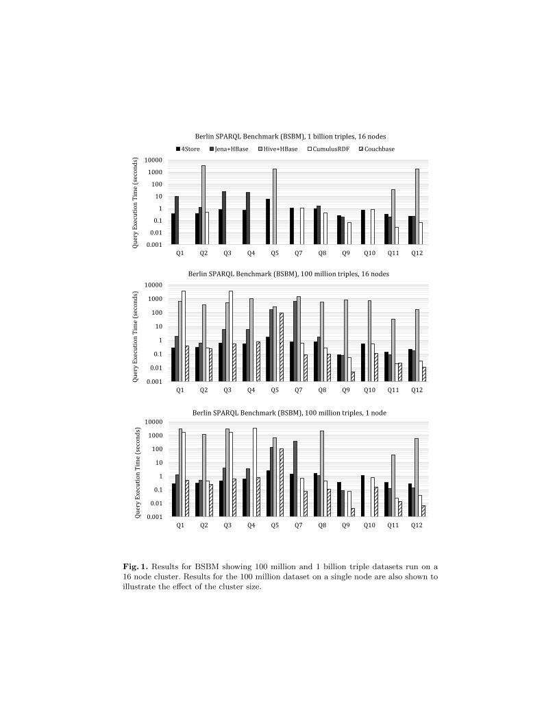
4store achieved sub-second response times for BSBM queries on 4, 8, and 16nodes with 10 and 100 million triples. The notable exception is Q5, which touchesa lot of data and contains a complex FILTER clause. Results for BSBM 1 billionare close to 1 second, except again for Q5 which takes between 6 seconds (16nodes) and 53 seconds (4 nodes). Overall, the system scales for BSBM as queryresponse times steadily decrease as the number of machines grow. Loading takesa few minutes, except for the 1 billion dataset which took 5.5 hours on 16 nodesand 14.9 hours on 8 nodes. Note: 4store actually times out when loading 1 billionfor 4 nodes but we still include the results to have a coherent baseline.

Results for the DBpedia SPARQL Benchmark are all in the same ballpark,with a median around 11 seconds when running on 4 nodes, 19 seconds whenrunning on 8, and 32 seconds when running on 16 nodes. We observe that the

18 http://ribs.csres.utexas.edu/nosqlrdf

Q1 Q2 Q3 Q4 Q5 Q7 Q8 Q9 Q10 Q11 Q12

0.001

0.01

0.1

1

10

100

1000

10000

Qu

ery

Exe

cuti

on

Tim

e (s

eco

nd

s)

Berlin SPARQL Benchmark (BSBM), 1 billion triples, 16 nodes

4Store Jena+HBase Hive+HBase CumulusRDF Couchbase

Q1 Q2 Q3 Q4 Q5 Q7 Q8 Q9 Q10 Q11 Q12

0.001

0.01

0.1

1

10

100

1000

10000

Qu

ery

Exe

cuti

on

Tim

e (s

eco

nd

s)

Berlin SPARQL Benchmark (BSBM), 100 million triples, 16 nodes

Q1 Q2 Q3 Q4 Q5 Q7 Q8 Q9 Q10 Q11 Q12

0.001

0.01

0.1

1

10

100

1000

10000

Qu

ery

Exe

cuti

on

Tim

e (s

eco

nd

s)

Berlin SPARQL Benchmark (BSBM), 100 million triples, 1 node

Fig. 1. Results for BSBM showing 100 million and 1 billion triple datasets run on a16 node cluster. Results for the 100 million dataset on a single node are also shown toillustrate the effect of the cluster size.

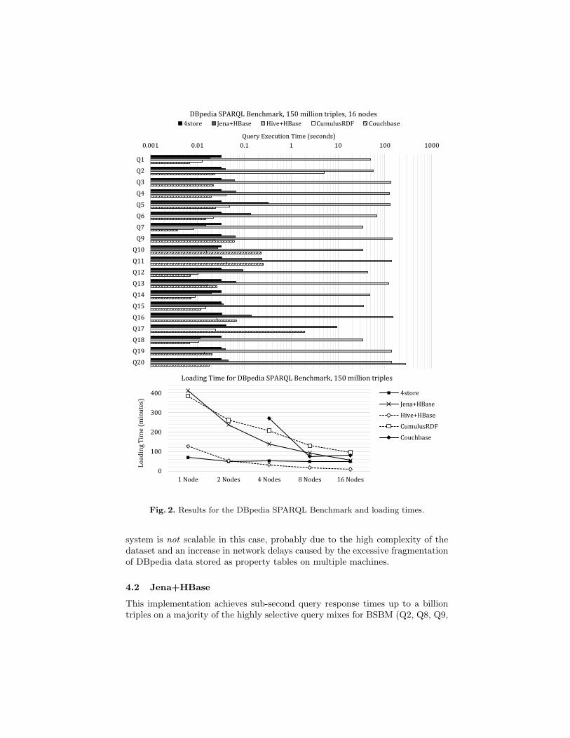
1 Node 2 Nodes 4 Nodes 8 Nodes 16 Nodes

0

100

200

300

400

Lo

adin

g T

ime

(min

ute

s)

Loading Time for DBpedia SPARQL Benchmark, 150 million triples

4store

Jena+HBase

Hive+HBase

CumulusRDF

Couchbase

Q1

Q2

Q3

Q4

Q5

Q6

Q7

Q9

Q10

Q11

Q12

Q13

Q14

Q15

Q16

Q17

Q18

Q19

Q20

0.001 0.01 0.1 1 10 100 1000

Query Execution Time (seconds)

DBpedia SPARQL Benchmark, 150 million triples, 16 nodes

4store Jena+HBase Hive+HBase CumulusRDF Couchbase

Fig. 2. Results for the DBpedia SPARQL Benchmark and loading times.

system is not scalable in this case, probably due to the high complexity of thedataset and an increase in network delays caused by the excessive fragmentationof DBpedia data stored as property tables on multiple machines.

4.2 Jena+HBase

This implementation achieves sub-second query response times up to a billiontriples on a majority of the highly selective query mixes for BSBM (Q2, Q8, Q9,

Q11, and Q12). This includes those queries that contain a variable predicate. Itis not relevant whether we have an inner or an outer join, instead results aregreatly influenced by selectivity. For low selectivity queries (Q1, Q3, Q10), we seethat leveraging HBase features is critical to even answer queries. For Q1 and Q3,we provide results for all dataset sizes. These two queries make use of numericalSPARQL filters which are pushed down as HBase prefix filters, whereas withQ10 we are unable to return results as it contains a date comparison filter whichhas not been pushed down. The importance of optimizing filters is also shownwhen a query touches a lot of data such as Q5, Q7 – both of which containcomplex or date specific filters.

In terms of the DBpedia SPARQL Benchmark, we see sub-second responsetimes for almost all queries. One reason is that our loading process eliminatesduplicates, which resulted in 60 million triples from the initial dataset beingstored. In addition, the queries tend to be much simpler than the BSBM queries.The one slower query (Q17) is again due to SPARQL filters on strings thatcould were not implemented as HBase filters. With filters pushed into HBase,the system approaches the performance of specially designed triple stores on amajority of queries. Still, we believe there is space for improvement in the joinstrategies as currently the “off-the-shelf” Jena strategy is used.

4.3 Hive+HBase

The implementation of Hive atop HBase introduces various sources of overheadfor query execution. As a result, query execution times are in the minute range.However, as more nodes are added to the cluster, query times are reduced.Additionally, initial load times tend to be fast.

For most queries, the MapReduce shuffle stage dominates the running time.Q7 is the slowest because it contains a 5-way join and requires 4 MapReducepasses from Hive. Currently, the system does not implement a query optimizerand it uses the naive Hive join algorithm19. For the DBpedia SPARQL Bench-mark, we observed faster query execution times than on BSBM. The datasetitself is more sparse than BSBM and the DBpedia queries are simpler; mostqueries do not involve a join. Due to the sparse nature of the dataset, bloomfilters allow us to scan less HDFS blocks. The simplicity of the queries reducenetwork traffic and also reduce time spent in the shuffle and reduce phases. How-ever, queries with language filters (e.g., Q3, Q9, Q11) perform slower since Hiveperforms a substring search for the requested SPARQL language identifier).

4.4 CumulusRDF: Cassandra+Sesame

For this implementation, the BSBM 1 billion dataset was only run on a 16node cluster. The loading time was 22 hours. All other cluster configurationsexceeded the loading timeout. For the 100 million dataset, the 2 node clusterbegan throwing exceptions midway in the benchmark. We observed that the

19 https://cwiki.apache.org/Hive/languagemanual-joins.html

system not only slowed down as more data was added but also as the clustersize increased. This could be attributed to the increased network communicationrequired by Cassandra in larger clusters. With parameter tuning, it may bepossible to reduce this. As expected, the loading time decreased as the clustersize increased.

BSBM queries 1, 3, 4, and 5 were challenging for the system. Some queriesexceeded the one hour time limit. For the 1 billion dataset, these same queriestimed out while most other queries executed in the sub-second range.

The DBpedia SPARQL Benchmark revealed three outliers: Q2, Q3, and Q20.Query 3 timed out for all cluster sizes. As the cluster size increased, the executiontime of query 2 and 20 increased as well. All other queries executed in the lowermillisecond range with minor increases in execution time as the cluster sizeincreased.

One hypothesis for the slow performance of the above queries is that, asopposed to other systems, CumulusRDF does not use a dictionary encoding forRDF constants. Therefore, joins require equality comparisons which are moreexpensive than numerical identifiers.

4.5 Couchbase

Couchbase encountered problems while loading the largest dataset, BSBM 1billion, which timed out on all cluster sizes. While the loading time for 8 and 16nodes is close to 24 hours, index generation in this case is very slow, hamperedby frequent node failures. Generating indices during loading was considerablyslower with smaller cluster sizes, where only part of the data can be held inmain memory (the index generation process took from less than an hour up tomore than 10 hours). The other two BSBM data sets, 10 million and 100 million,were loaded on every cluster configuration with times ranging from 12 minutes(BSBM 10 million, 8 nodes) to over 3.5 hours (100 million, 1 node). In the caseof DBpedia, there are many duplicate triples spread across the data set, whichcause many read operations and thus slower loading times. Also, the uneven sizeof molecules and triples caused frequent node failures during index creation. Forthis reason, we only report results with 4 clusters and more, where the loadingtimes range from 74 min for 8 nodes to 4.5 hours for 4 nodes.

Overall, query execution is relatively fast. Queries take between 4 ms (Q9)and 104 seconds (Q5) for BSBM 100 million. As noted above, Q5 touches a lot ofdata and contains a complex FILTER clause, which leads to a very high numberof database accesses in our case, since none of the triple patterns of the query isvery restrictive. As the cluster size increases, the query execution times remainrelatively constant. Results for DBpedia benchmark exhibit similar trends.

5 Related Work

Benchmarking has been a core topic of RDF data management research. Inaddition to BSBM and the DBpedia benchmark, SP2Bench [16] and LUBM

[6] are widely used benchmarks. Our paper aims to use these benchmarks toinvestigate NoSQL stores that were not originally intended for RDF. Indexingand storage schemas have a large impact on the performance of a database.Sidirourgos et al. [17] use a single system to evaluate the performance impactof different approaches. Again, our paper looks at multiple, widely used, andcurrently deployed NoSQL systems.

Of the NoSQL systems available, HBase has been the most widely used.Jianling Sun [18] adopted the Hexastore [23] schema for HBase by storing verboseRDF data. Papailiou et. al. [13] developed H2RDF, a distributed triple-storealso based on HBase. Khadilkar et al. [22] developed several versions of a triplestore that combines the Jena framework with the storage provided by HBase.Przyjaciel-Zablocki et al. [15] created a scalable technique for doing indexednested loop joins which combines the power of the MapReduce paradigm withthe random access pattern provided by HBase.

Another important category for NoSQL RDF storage is the concept of graphdatabases. Most triple stores (i.e. 4store) can be seen as an implementation of agraph database. Popular products include Virtuoso20, Neo4j21, AllegroGraph22,and Bigdata23.

An interesting direction forward for NoSQL stores is presented by Tsialia-manis et. al [19]. Using the MonetDB column-store, they show heuristics forefficient SPARQL query planning without using statistics which add overheadin terms of maintainability, storage space, and query execution.

6 Conclusions

This paper represents, to the best of our knowledge, the first systematic attemptat characterizing and comparing NoSQL stores for RDF processing. The systemswe have evaluated above all exhibit their own strengths and weaknesses. Overall,we can make a number of key observations:

1. Distributed NoSQL systems can be competitive against distributed and na-tive RDF stores (such as 4store) with respect to query times. Relativelysimple SPARQL queries such as distributed lookups, in particular, can be ex-ecuted very efficiently on such systems, even for larger clusters and datasets.For example, on BSBM 1 billion triples, 16 nodes, Q9, Q11, and Q12 areprocessed more efficiently on Cassandra and Jena+HBase than on 4store.

2. Loading times for RDF data varies depending on the NoSQL system andindexing approach used. However, we observe that most of the NoSQL sys-tems scale more gracefully than the native RDF store when loading data inparallel.

20 http://virtuoso.openlinksw.com/21 http://www.neo4j.org/22 http://www.franz.com/agraph/allegrograph/23 http://www.systap.com/bigdata.htm

3. More complex SPARQL queries involving several joins, touching a lot ofdata, or containing complex filters perform, generally-speaking, poorly onNoSQL systems. Take the following queries for example: BSBM Q3 containsa negation, Q4 contains a union, and Q5 touches a lot of data and has acomplex filter. These queries run considerably slower on NoSQL systemsthan on 4store.

4. Following the comment above, we observe that classical query optimizationtechniques borrowed from relational databases generally work well on NoSQLRDF systems. Jena+HBase, for example, performs better than other systemson many join and filter queries since it reorders the joins, pushes down theselections and filters in its query plans.

5. MapReduce-like operations introduce a higher latency for distributed viewmaintenance and query execution times. For instance, Hive+HBase andCouchbase (on larger clusters) introduce large amounts of overhead resultingin slower runtimes.

In conclusion, NoSQL systems represent a compelling alternative to distributedand native RDF stores for simple workloads. Considering the encouraging resultsfrom this study, the very large user base of NoSQL systems, and the fact thatthere is still ample room for query optimization techniques, we are confident thatNoSQL databases will present an ever growing opportunity to store and manageRDF data in the cloud.

Acknowledgements The work on Jena+HBase was supported by the Innovative

Medicines Initiative Joint Undertaking under grant agreement number 115191. The

work on Hive+HBase was supported by the United States National Science Foun-

dation Grant IIS-1018554. The work on CumulusRDF was partially supported by

the European Commission’s Seventh Framework Programme (PlanetData NoE, grant

257641). The work on Couchbase was supported by the Swiss NSF under grant number

PP00P2 128459.

References

1. Abadi, D.J., Marcus, A., Madden, S.R., Hollenbach, K.: Scalable semantic web datamanagement using vertical partitioning. In: Proceedings of the 33rd internationalconference on Very large data bases. pp. 411–422. VLDB ’07 (2007)

2. Bizer, C., Schultz, A.: The berlin sparql benchmark. International Journal on Se-mantic Web and Information Systems (IJSWIS) 5(2), 1–24 (2009)

3. Chang, F., Dean, J., Ghemawat, S., Hsieh, W.C., Wallach, D.A., Burrows, M.,Chandra, T., Fikes, A., Gruber, R.E.: Bigtable: A distributed storage system forstructured data. ACM Trans. Comput. Syst. 26(2), 4:1–4:26 (Jun 2008)

4. Fundatureanu, S.: A Scalable RDF Store Based on HBase. Master’s thesis, VrijeUniversity (2012), http://archive.org/details/ScalableRDFStoreOverHBase

5. Gueret, C., Kotoulas, S., Groth, P.: Triplecloud: An infrastructure for exploratoryquerying over web-scale rdf data. WI-IAT (2011)

6. Guo, Y., Pan, Z., Heflin, J.: Lubm: A benchmark for owl knowledge base systems.Web Semantics: Science, Services and Agents on the World Wide Web (2005)

7. Harris, S., Lamb, N., Shadbolt, N.: 4store: The design and implementation of aclustered rdf store. In: 5th International Workshop on Scalable Semantic WebKnowledge Base Systems (SSWS2009). pp. 94–109 (2009)

8. Harth, A., Decker, S.: Optimized Index Structures for Querying RDF from theWeb. In: IEEE LA-WEB. pp. 71–80 (2005)

9. Ladwig, G., Harth, A.: CumulusRDF: Linked data management on nested key-value stores. In: The 7th International Workshop on Scalable Semantic Web Knowl-edge Base Systems (SSWS 2011). p. 30 (2011)

10. Lakshman, A., Malik, P.: Cassandra: a decentralized structured storage system.SIGOPS Oper. Syst. Rev. 44(2), 35–40 (Apr 2010)

11. Morsey, M., Lehmann, J., Auer, S., Ngomo, A.C.N.: Dbpedia sparql benchmark–performance assessment with real queries on real data. In: The Semantic Web–ISWC 2011, pp. 454–469. Springer (2011)

12. O’Malley, O.: Terabyte sort on apache hadoop (2008), http://sortbenchmark.

org/YahooHadoop.pdf

13. Papailiou, N., Konstantinou, I., Tsoumakos, D., Koziris, N.: H2rdf: adaptive queryprocessing on rdf data in the cloud. In: WWW (Companion Volume)

14. Pokorny, J.: Nosql databases: a step to database scalability in web environment.In: Proceedings of the 13th International Conference on Information Integrationand Web-based Applications and Services. pp. 278–283. iiWAS ’11, ACM, NewYork, NY, USA (2011)

15. Przyjaciel-Zablocki, M., Schatzle, A., Hornung, T., Dorner, C., Lausen, G.: Cas-cading map-side joins over hbase for scalable join processing. CoRR (2012)

16. Schmidt, M., Hornung, T., Kuchlin, N., Lausen, G., Pinkel, C.: An experimentalcomparison of rdf data management approaches in a sparql benchmark scenario.In: Proceedings of the 7th International Conference on The Semantic Web. pp.82–97. ISWC ’08, Springer-Verlag, Berlin, Heidelberg (2008)

17. Sidirourgos, L., Goncalves, R., Kersten, M., Nes, N., Manegold, S.: Column-storesupport for rdf data management: not all swans are white. Proc. VLDB Endow.1(2), 1553–1563 (Aug 2008)

18. Sun, J.: Scalable rdf store based on hbase and mapreduce. In: Advanced ComputerTheory and Engineering (ICACTE), 2010 3rd International Conference

19. Tsialiamanis, P., Sidirourgos, L., Fundulaki, I., Christophides, V., Boncz, P.:Heuristics-based query optimisation for sparql. In: Proceedings of the 15th In-ternational Conference on Extending Database Technology

20. Urbani, J., Kotoulas, S., Maassen, J., Drost, N., Seinstra, F., Harmelen, F.V.,Bal, H.: H.: Webpie: A web-scale parallel inference engine. In: In: Third IEEEInternational Scalable Computing Challenge (SCALE2010), held in conjunctionwith the 10th IEEE/ACM International Symposium on Cluster, Cloud and GridComputing (CCGrid) (2010)

21. Urbani, J., Van Harmelen, F., Schlobach, S., Bal, H.: Querypie: Backward reasoningfor owl horst over very large knowledge bases. In: The Semantic Web–ISWC 2011,pp. 730–745. Springer (2011)

22. Vaibhav Khadilkar, Murat Kantarcioglu, B.T., Castagna, P.: Jena-hbase: A dis-tributed, scalable and efficient rdf triple store. In: Proceedings of the ISWC 2012Posters & Demonstrations Track (2012)

23. Weiss, C., Karras, P., Bernstein, A.: Hexastore: sextuple indexing for semantic webdata management. Proc. VLDB Endow. (2008)