note to the trainer: these slides are provided to standardize crews to collect ozone indicator data....
TRANSCRIPT
Note to the Trainer:
These slides are provided to standardize crews to collect ozone indicator data. The first 50 slides are introductory. You may decide not to use all of these slides, but the following concepts must be emphasized.
1. Provide visual evidence that ambient ozone concentrations are high across your sampling area. It is best to locate a current, regional map from the EPA web site, but if this is not possible, use the national map provided in slide #14. http://www.epa.gov/air/data/index.html
2. Clarify the Training Objectives. Review or adapt slides #4 and #5 to your session.
3. Clarify the distinction between the beneficial ozone layer and ground level ozone pollution.
4. Provide some indication as to why the ozone indicator is important to FIA and to the country as in slides #36, #37, #38. See slides #16, #17, #18, #19 as well.
5. Provide some evidence of state-level results from your own region if possible.
6. Do not abbreviate the procedural slides included here and numbered slides #52 - #105.
7. The symptom review slides are in a separate file. Review the species that are used in your region and focus on the best slides. There is a third file that provides 16 ozone injury slides for testing the trainees and/or for additional review and discussion.
The slides will load faster if they are first copied from the CD to your hard drive. You should then be able to edit them as you see fit.

1 - 50Good
51 - 100Moderate
101 - 150Unhealthy forSensitive Groups
151 - 200Unhealthy
201 - 250Very Unhealthy
Green = Good
Yellow = Moderate
Orange = Unhealthy for Sensitive Groups
Red = Unhealthy
Purple = Very Unhealthy
Air Quality Guide (ppb O3)
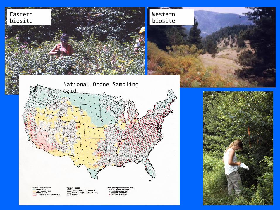
Eastern biosite Western biosite
National Ozone Sampling Grid
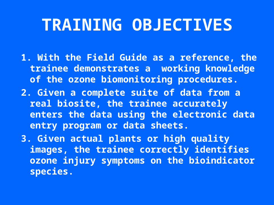
TRAINING OBJECTIVES
1. With the Field Guide as a reference, the trainee demonstrates a working knowledge of the ozone biomonitoring procedures.
2. Given a complete suite of data from a real biosite, the trainee accurately enters the data using the electronic data entry program or data sheets.
3. Given actual plants or high quality images, the trainee correctly identifies ozone injury symptoms on the bioindicator species.
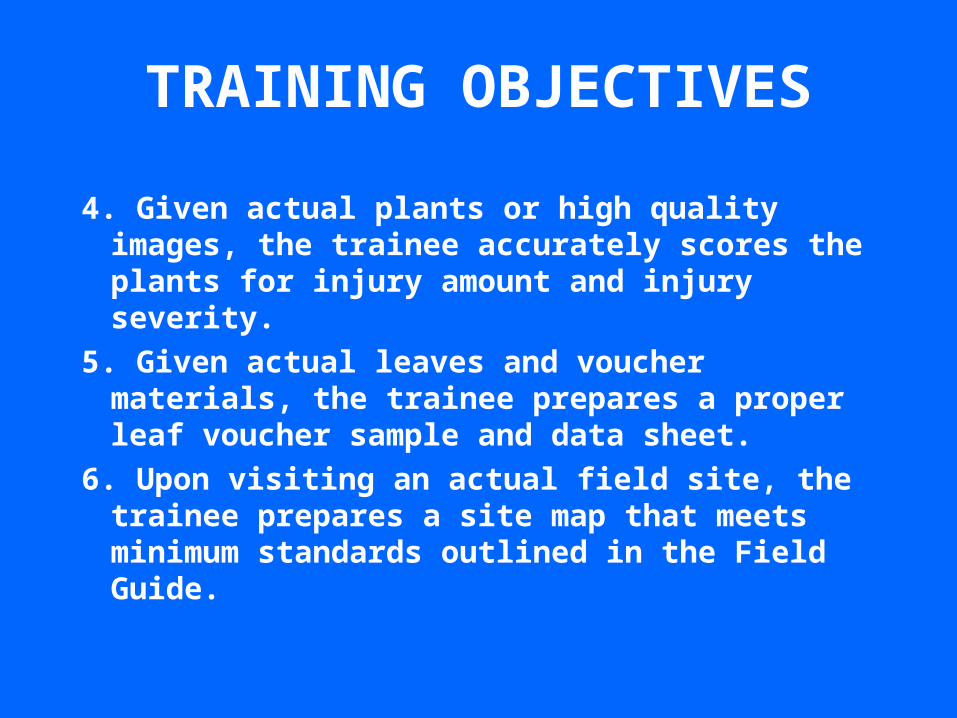
4. Given actual plants or high quality images, the trainee accurately scores the plants for injury amount and injury severity.
5. Given actual leaves and voucher materials, the trainee prepares a proper leaf voucher sample and data sheet.
6. Upon visiting an actual field site, the trainee prepares a site map that meets minimum standards outlined in the Field Guide.
TRAINING OBJECTIVES

OZONE TRAINING AGENDAMorning Session: inside 8:00 to 11:30
• Introduction - Why do we do it?
• Field Procedures - How do we do it?
• Symptom Review - What does ozone injury look like?
• Written Test** - What information is in the Field Guide?
• Electronic Data Entry and Data Sheets
• Plot Location Check – State Crosswalk Tables
LUNCH
**requires a passing grade for certification
OZONE TRAINING AGENDAAfternoon Session: outside 1:00 to 4:00
• Field exercise - What does a biosite look like?
• Review of species ID and plant selection
• Review of symptom identification and scoring
• Biosite map - How is biosite location documented?
• Voucher handling - How are injury symptoms validated?
• Review of QA activities
• Debriefing Form
• Distribution of field supplies
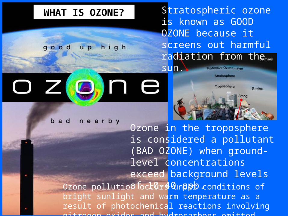
Stratospheric ozone is known as GOOD OZONE because it screens out harmful radiation from the sun.
Ozone in the troposphere is considered a pollutant (BAD OZONE) when ground-level concentrations exceed background levels of 10-40 ppb.
Ozone pollution occurs under conditions of bright sunlight and warm temperature as a result of photochemical reactions involving nitrogen oxides and hydrocarbons emitted from cars and industry.
WHAT IS OZONE?
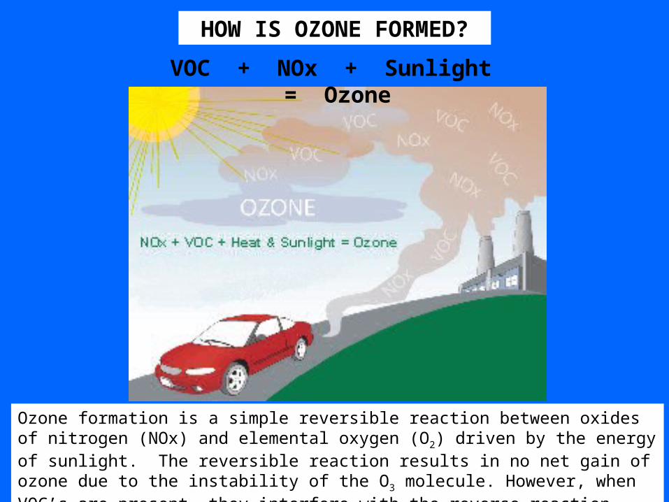
VOC + NOx + Sunlight = Ozone
Ozone formation is a simple reversible reaction between oxides of nitrogen (NOx) and elemental oxygen (O2) driven by the energy of sunlight. The reversible reaction results in no net gain of ozone due to the instability of the O3 molecule. However, when VOC’s are present, they interfere with the reverse reaction resulting in a build-up of ozone in ambient air.
HOW IS OZONE FORMED?
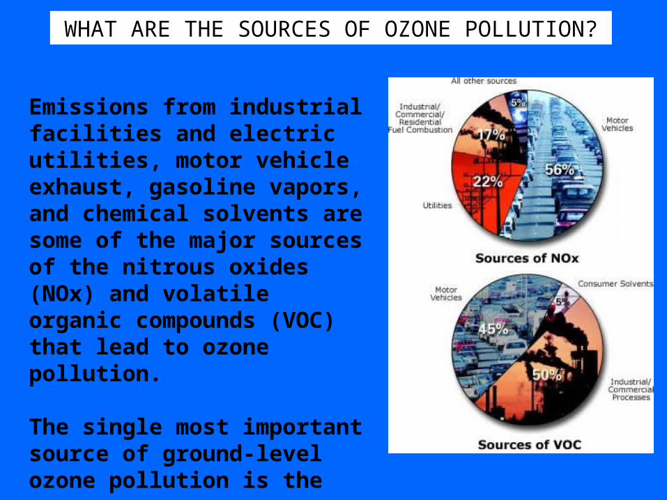
Emissions from industrial facilities and electric utilities, motor vehicle exhaust, gasoline vapors, and chemical solvents are some of the major sources of the nitrous oxides (NOx) and volatile organic compounds (VOC) that lead to ozone pollution.
The single most important source of ground-level ozone pollution is the car.
WHAT ARE THE SOURCES OF OZONE POLLUTION?
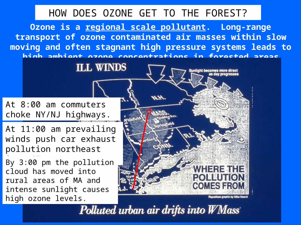
Ozone is a regional scale pollutant. Long-range transport of ozone contaminated air masses within slow moving and often stagnant high pressure systems leads to high ambient ozone concentrations in forested areas downwind of urban centers.
At 8:00 am commuters choke NY/NJ highways.
At 11:00 am prevailing winds push car exhaust pollution northeast into CT
By 3:00 pm the pollution cloud has moved into rural areas of MA and intense sunlight causeshigh ozone levels.
HOW DOES OZONE GET TO THE FOREST?
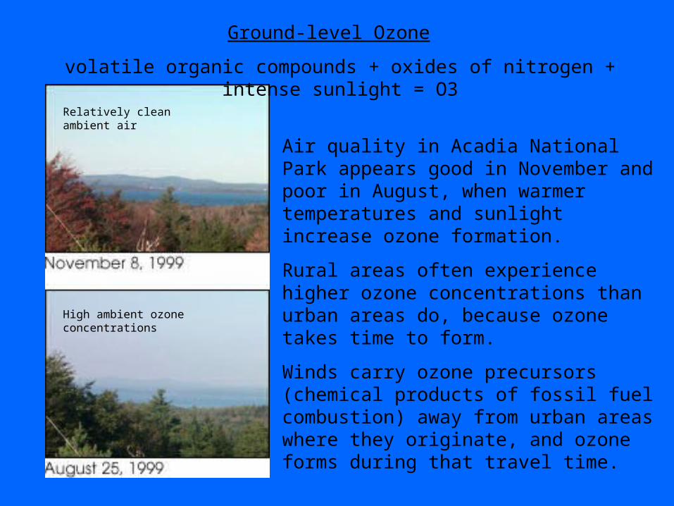
Air quality in Acadia National Park appears good in November and poor in August, when warmer temperatures and sunlight increase ozone formation.
Rural areas often experience higher ozone concentrations than urban areas do, because ozone takes time to form.
Winds carry ozone precursors (chemical products of fossil fuel combustion) away from urban areas where they originate, and ozone forms during that travel time.
Ground-level Ozone
volatile organic compounds + oxides of nitrogen + intense sunlight = O3
Relatively clean ambient air
High ambient ozone concentrations
Day 1
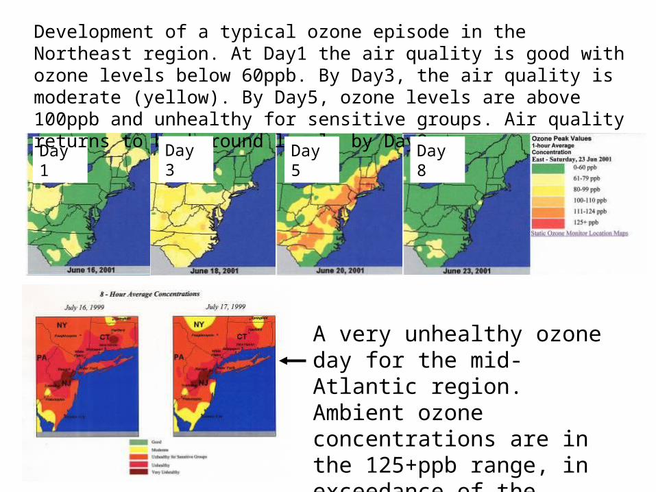
Development of a typical ozone episode in the Northeast region. At Day1 the air quality is good with ozone levels below 60ppb. By Day3, the air quality is moderate (yellow). By Day5, ozone levels are above 100ppb and unhealthy for sensitive groups. Air quality returns to background levels by Day8.
Day 3 Day 5 Day 8
A very unhealthy ozone day for the mid-Atlantic region. Ambient ozone concentrations are in the 125+ppb range, in exceedance of the National Ambient Air Quality Standard.
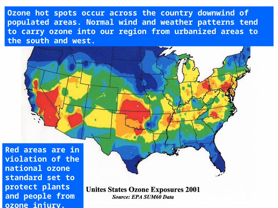
Ozone hot spots occur across the country downwind of populated areas. Normal wind and weather patterns tend to carry ozone into our region from urbanized areas to the south and west.
Red areas are in violation of the national ozone standard set to protect plants and people from ozone injury.
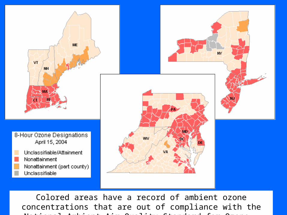
Colored areas have a record of ambient ozone concentrations that are out of compliance with the National Ambient Air Quality Standard for Ozone.
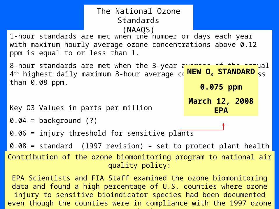
1-hour standards are met when the number of days each year with maximum hourly average ozone concentrations above 0.12 ppm is equal to or less than 1.
8-hour standards are met when the 3-year average of the annual 4th highest daily maximum 8-hour average concentration is less than 0.08 ppm.
Key O3 Values in parts per million
0.04 = background (?)
0.06 = injury threshold for sensitive plants
0.08 = standard (1997 revision) – set to protect plant health
0.12 = older 1 hour standard in place since 1979
The National Ozone Standards(NAAQS)
NEW O3 STANDARD
0.075 ppm
March 12, 2008 EPA
Contribution of the ozone biomonitoring program to national air quality policy:
EPA Scientists and FIA Staff examined the ozone biomonitoring data and found a high percentage of U.S. counties where ozone injury to sensitive bioindicator species had been documented even though the counties were in compliance with the 1997 ozone standard.
Conclusion: The ozone standard needed to be strengthened.
No ChangeNo Change401-500
No ChangeNo Change301-400Hazardous
0.116-0.3740.125-0.374201-300Very
Unhealthy
0.096-0.1150.105-0.124151-200Unhealthy
0.076-0.0950.085-0.104101-150
Unhealthy for
Sensitive Groups
0.060-0.0750.065-0.08451-100Moderate
0.000-0.0590.000-0.0640-50Good
20088-hour(ppm)
19978-hour(ppm)
AQI Value
Category
Revised Ozone AQI Breakpoints, 2008
For more information about EPA’s action to strengthen the national ozone standards: www.epa.gov/groundlevelozone.
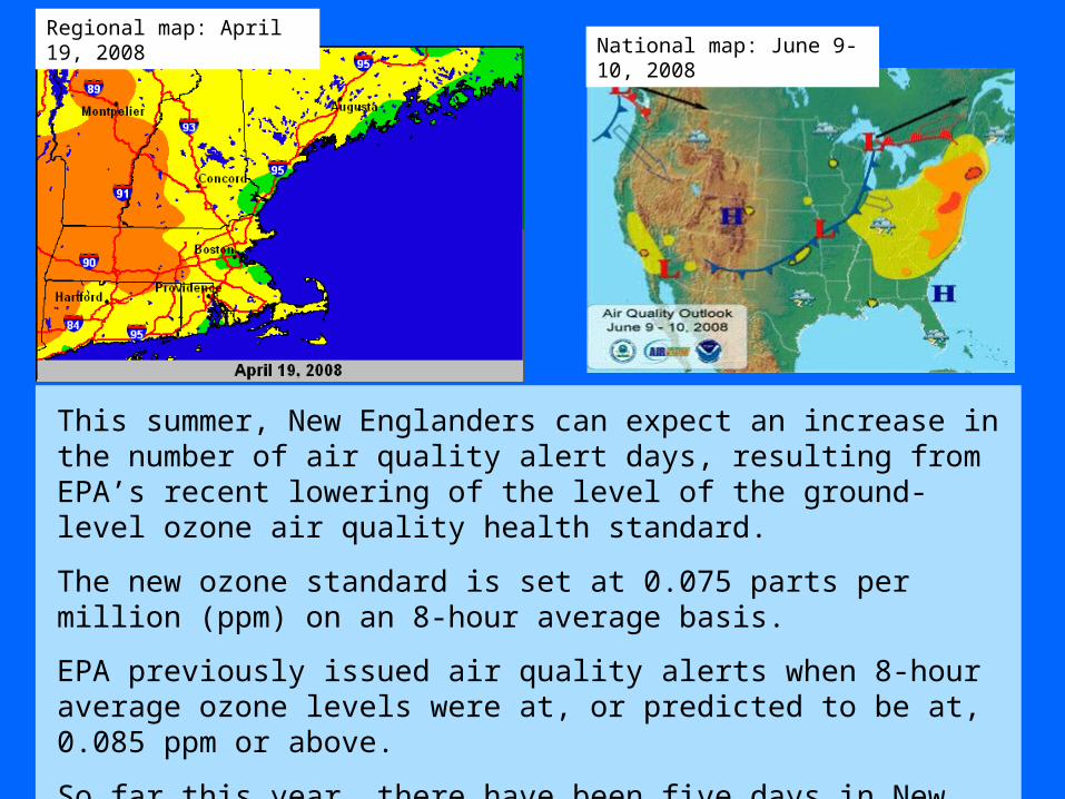
This summer, New Englanders can expect an increase in the number of air quality alert days, resulting from EPA’s recent lowering of the level of the ground-level ozone air quality health standard.
The new ozone standard is set at 0.075 parts per million (ppm) on an 8-hour average basis.
EPA previously issued air quality alerts when 8-hour average ozone levels were at, or predicted to be at, 0.085 ppm or above.
So far this year, there have been five days in New England when ozone concentrations have exceeded the new ozone standard.
National map: June 9-10, 2008Regional map: April 19, 2008
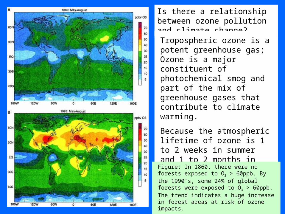
Is there a relationship between ozone pollution and climate change?
Tropospheric ozone is a potent greenhouse gas; Ozone is a major constituent of photochemical smog and part of the mix of greenhouse gases that contribute to climate warming.
Because the atmospheric lifetime of ozone is 1 to 2 weeks in summer and 1 to 2 months in winter, ozone produced in a polluted region of one continent can be transported to another continent all year long.
Figure: In 1860, there were no forests exposed to O3 > 60ppb. By the 1990’s, some 24% of global forests were exposed to O3 > 60ppb. The trend indicates a huge increase in forest areas at risk of ozone impacts.
Monitoring needs are paramount.
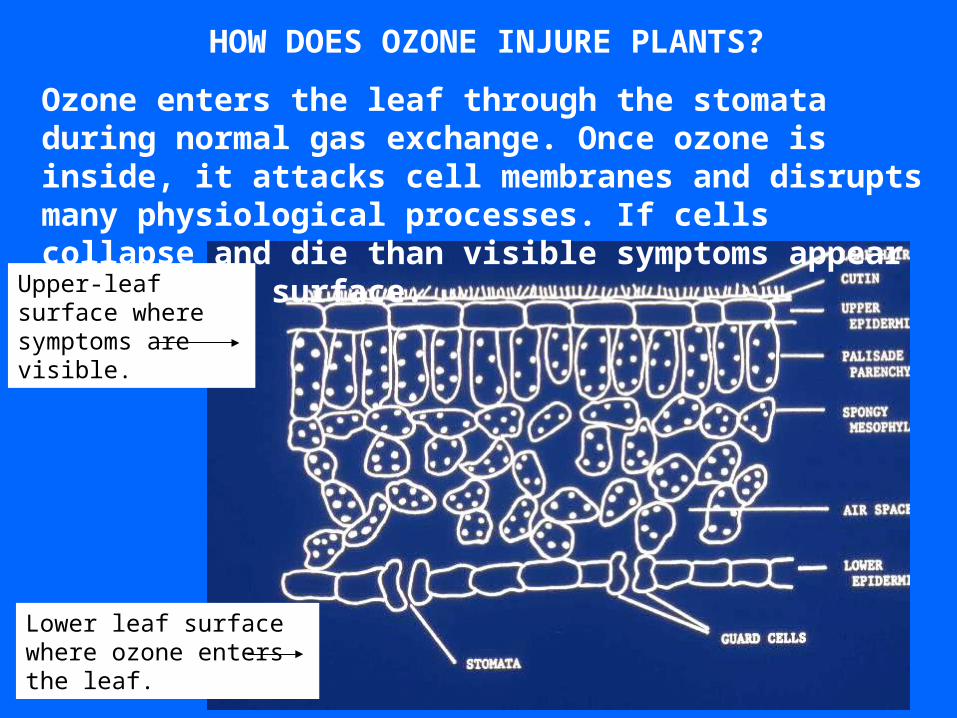
HOW DOES OZONE INJURE PLANTS?
Ozone enters the leaf through the stomata during normal gas exchange. Once ozone is inside, it attacks cell membranes and disrupts many physiological processes. If cells collapse and die than visible symptoms appear on the leaf surface.
Upper-leaf surface where symptoms are visible.
Lower leaf surface where ozone enters the leaf.
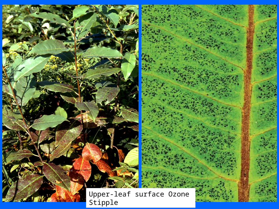
Upper-leaf surface Ozone Stipple
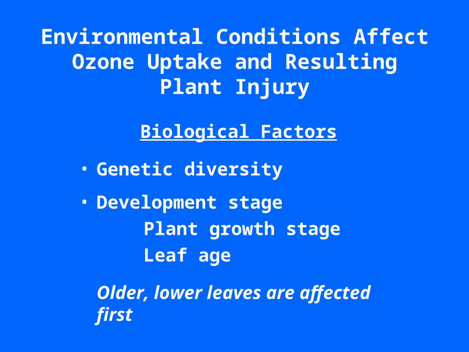
Environmental Conditions Affect Ozone Uptake and Resulting Plant Injury
Biological Factors
• Genetic diversity
• Development stage
Plant growth stage
Leaf age
Older, lower leaves are affected first
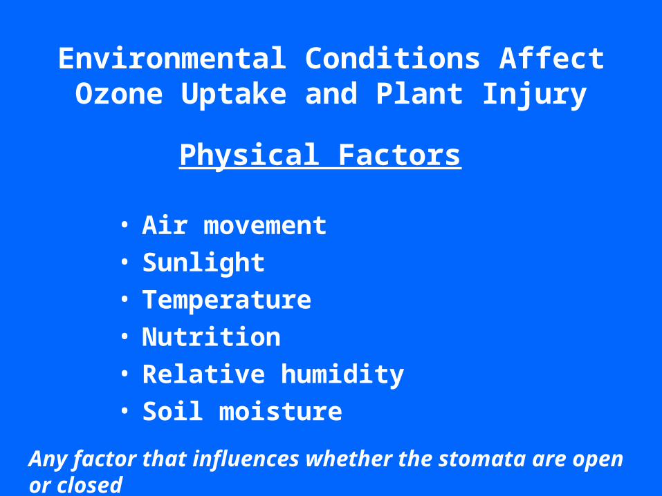
Environmental Conditions Affect Ozone Uptake and Plant Injury
Physical Factors
• Air movement• Sunlight• Temperature• Nutrition• Relative humidity• Soil moisture
Any factor that influences whether the stomata are open or closed
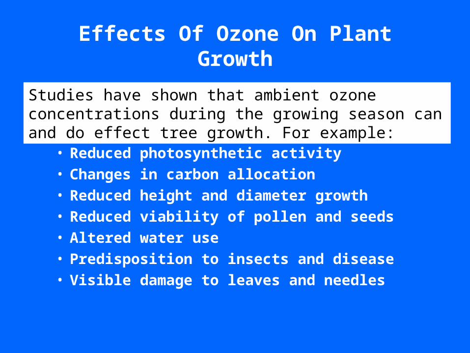
Effects Of Ozone On Plant Growth
• Reduced photosynthetic activity• Changes in carbon allocation• Reduced height and diameter growth• Reduced viability of pollen and seeds• Altered water use• Predisposition to insects and disease• Visible damage to leaves and needles
Studies have shown that ambient ozone concentrations during the growing season can and do effect tree growth. For example:
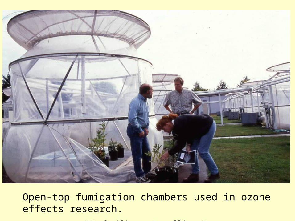
Open-top fumigation chambers used in ozone effects research.
EPA facility - Corvallis, OR.
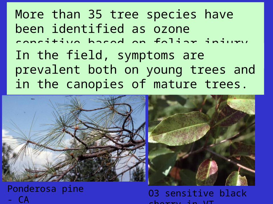
More than 35 tree species have been identified as ozone sensitive based on foliar injury symptoms.
Ponderosa pine - CA O3 sensitive black cherry in VT
In the field, symptoms are prevalent both on young trees and in the canopies of mature trees.
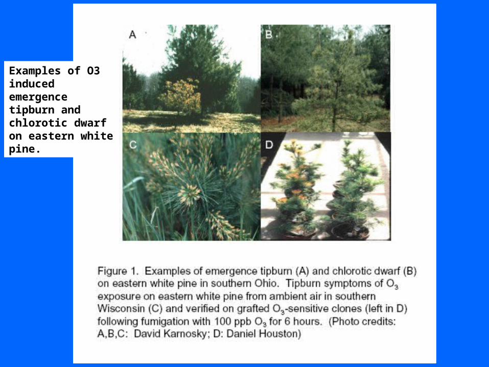
Examples of O3 induced emergence tipburn and chlorotic dwarf on eastern white pine.
O3 haze
O3 chlorotic mottle
O3 thin crown
Bark beetle attack
0
1
2
3
4
5
0 20 40 60 80
Chlorotic Mottle(percent of total surface area)
Net P
ho
tosyn
thesis
(um
ol m
-2 s
-1)
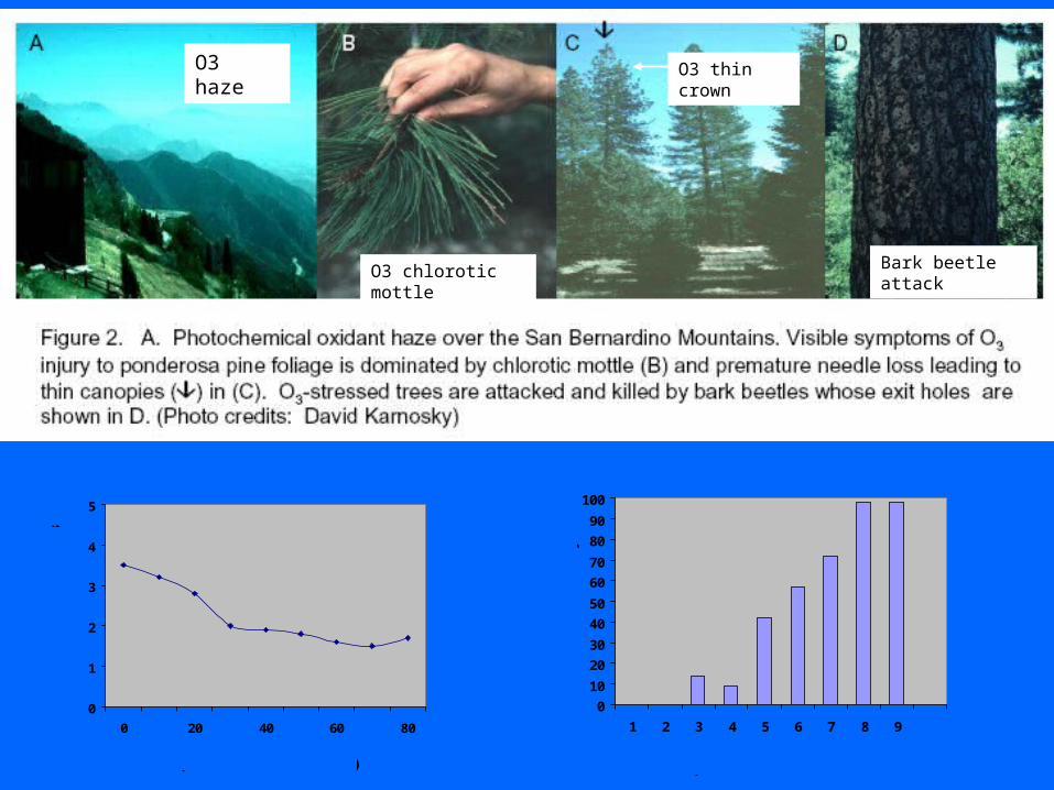
Relationship between severity of chlorotic mottle and net photosynthesis in Jeffrey pine under conditions of adequate soil mositure.
0
10
20
30
40
50
60
70
80
90
100
1 2 3 4 5 6 7 8 9
Perc
en
t M
ort
alit
y
Numerical Rating of Symptoms1 = healthy; 2-4 = intermediate; 5-9 = advanced
Mortality of ozone injured ponderosa pines in relation to numerical rating of symptoms.
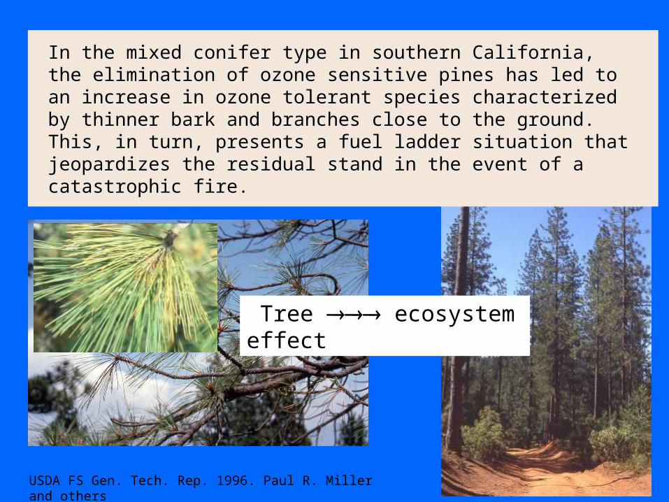
In the mixed conifer type in southern California, the elimination of ozone sensitive pines has led to an increase in ozone tolerant species characterized by thinner bark and branches close to the ground. This, in turn, presents a fuel ladder situation that jeopardizes the residual stand in the event of a catastrophic fire.
Tree ecosystem effect
USDA FS Gen. Tech. Rep. 1996. Paul R. Miller and others
sensitive
intermediatetolerant
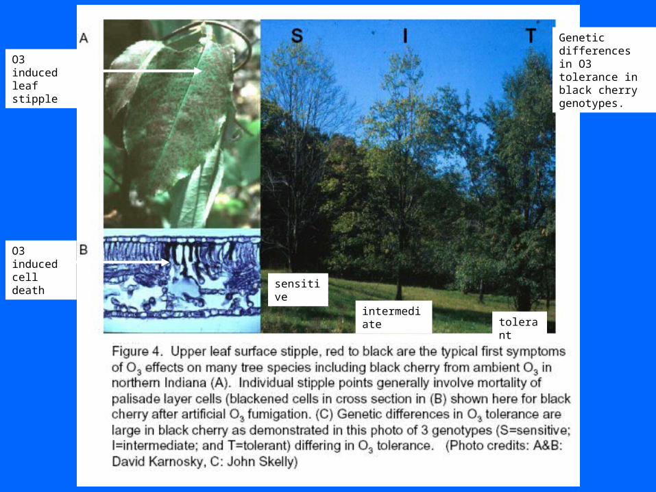
O3 induced cell death
O3 induced leaf stipple
Genetic differences in O3 tolerance in black cherry genotypes.
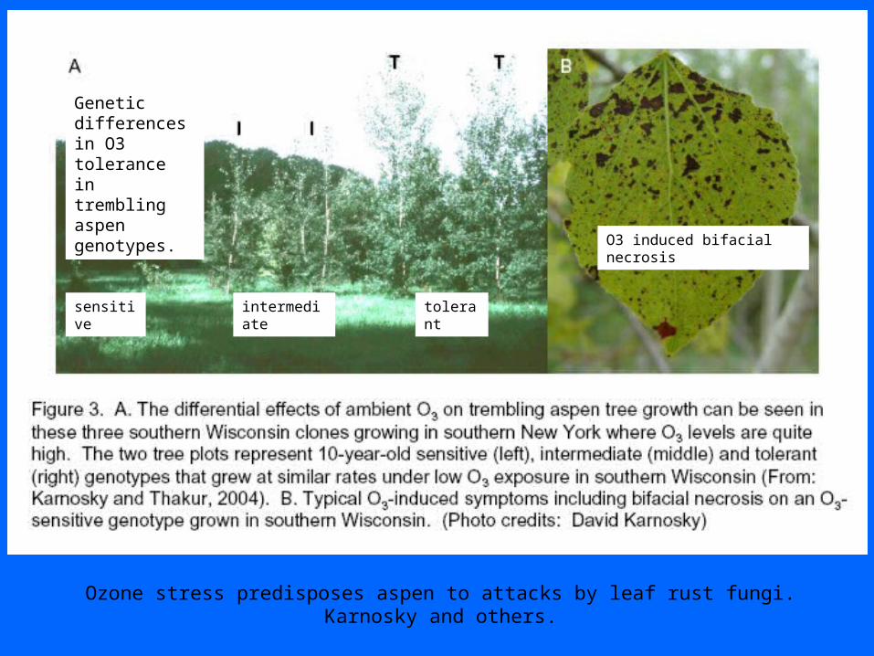
Genetic differences in O3 tolerance in trembling aspen genotypes.
sensitive intermediate tolerant
O3 induced bifacial necrosis
Ozone stress predisposes aspen to attacks by leaf rust fungi. Karnosky and others.
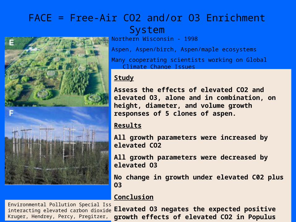
FACE = Free-Air CO2 and/or O3 Enrichment System
Northern Wisconsin - 1998
Aspen, Aspen/birch, Aspen/maple ecosystems
Many cooperating scientists working on Global Climate Change Issues
Environmental Pollution Special Issue: Growth responses of Populus tremuloides clones to interacting elevated carbon dioxide and tropospheric ozone. 2001. Isebrands, McDonald, Kruger, Hendrey, Percy, Pregitzer, Sober, Karnosky.
Study
Assess the effects of elevated CO2 and elevated O3, alone and in combination, on height, diameter, and volume growth responses of 5 clones of aspen.
Results
All growth parameters were increased by elevated CO2
All growth parameters were decreased by elevated O3
No change in growth under elevated C02 plus O3
Conclusion
Elevated O3 negates the expected positive growth effects of elevated CO2 in Populus tremuloides.
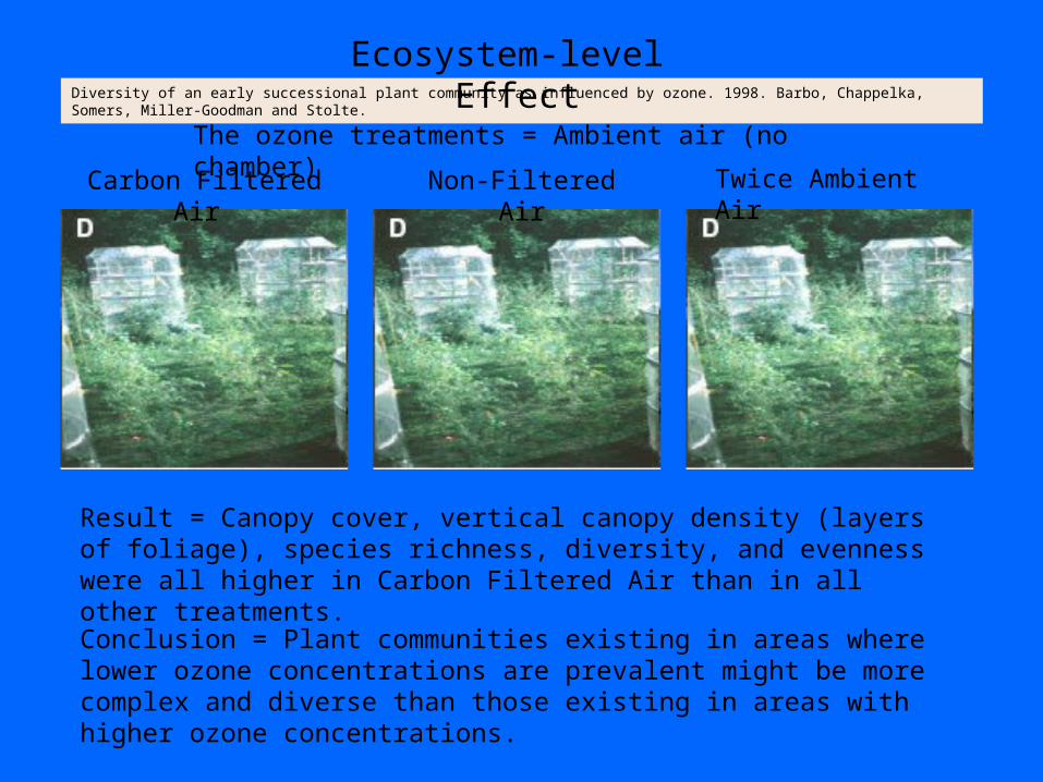
The ozone treatments = Ambient air (no chamber)
Carbon Filtered Air Non-Filtered Air Twice Ambient Air
Result = Canopy cover, vertical canopy density (layers of foliage), species richness, diversity, and evenness were all higher in Carbon Filtered Air than in all other treatments.
Conclusion = Plant communities existing in areas where lower ozone concentrations are prevalent might be more complex and diverse than those existing in areas with higher ozone concentrations.
Diversity of an early successional plant community as influenced by ozone. 1998. Barbo, Chappelka, Somers, Miller-Goodman and Stolte.
Ecosystem-level Effect
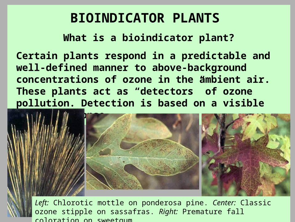
BIOINDICATOR PLANTS
What is a bioindicator plant?
Certain plants respond in a predictable and well-defined manner to above-background concentrations of ozone in the ambient air. These plants act as “detectors” of ozone pollution. Detection is based on a visible foliar response.
Left: Chlorotic mottle on ponderosa pine. Center: Classic ozone stipple on sassafras. Right: Premature fall coloration on sweetgum.
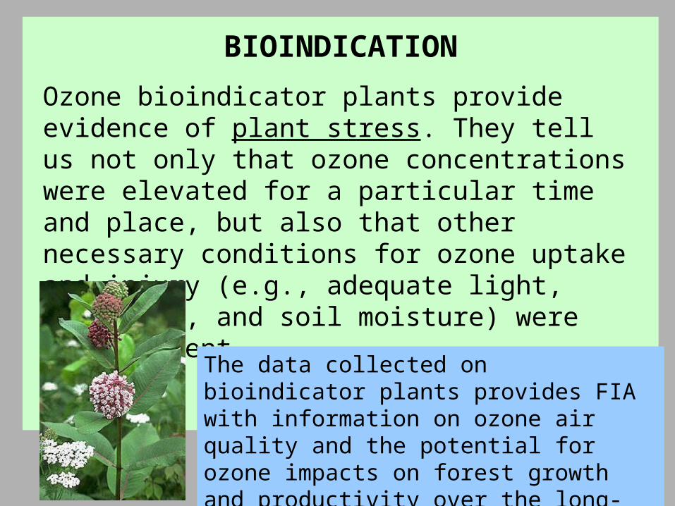
BIOINDICATION
Ozone bioindicator plants provide evidence of plant stress. They tell us not only that ozone concentrations were elevated for a particular time and place, but also that other necessary conditions for ozone uptake and injury (e.g., adequate light, nutrition, and soil moisture) were also present.
The data collected on bioindicator plants provides FIA with information on ozone air quality and the potential for ozone impacts on forest growth and productivity over the long-term.
Why is the ozone indicator important?
The USDA Forest Service made a commitment to the international community to monitor the area and percent of forestland subjected to levels of specific air pollutants, including ozone, which may cause negative impacts on the forest ecosystem.
The FIA biomonitoring program is the only large-scale effort to monitor ozone stress in the natural environment.
1. TO MEET USFS INITIATIVES
FIA Detection Monitoring and the1995 Santiago Agreement
Why is the ozone indicator important?
There is a recognized need for biological data that can help inform and influence the establishment of meaningful air quality standards to protect plants from ozone damage.
The scientific community says foliar injury data from natural systems is a priority research need.
The FIA biomonitoring program meets that need.
2. TO SUPPORT NATIONAL POLICY ON
PLANT HEALTH PROTECTION
Why is the ozone indicator important?
Model simulations are the only way we can get close to interpreting the risks associated with long-term ozone exposures.
Biomonitoring data provides more, different, and better data that will improve the reliability of forest health models.
3. TO IMPROVE FOREST HEALTH - RISK ASSESSEMNT MODELS
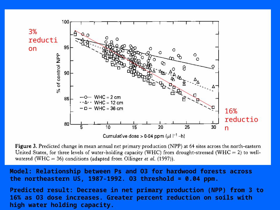
3% reduction
16% reduction
Model: Relationship between Ps and O3 for hardwood forests across the northeastern US, 1987-1992. O3 threshold = 0.04 ppm.
Predicted result: Decrease in net primary production (NPP) from 3 to 16% as O3 dose increases. Greater percent reduction on soils with high water holding capacity.
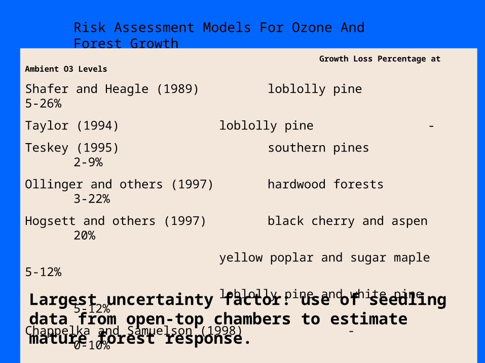
Risk Assessment Models For Ozone And Forest Growth
Growth Loss Percentage at Ambient O3 Levels
Shafer and Heagle (1989) loblolly pine 5-26%
Taylor (1994) loblolly pine -
Teskey (1995) southern pines 2-9%
Ollinger and others (1997) hardwood forests 3-22%
Hogsett and others (1997) black cherry and aspen 20%
yellow poplar and sugar maple 5-12%
loblolly pine and white pine 5-12%
Chappelka and Samuelson (1998) - 0-10%
Largest uncertainty factor: use of seedling data from open-top chambers to estimate mature forest response.
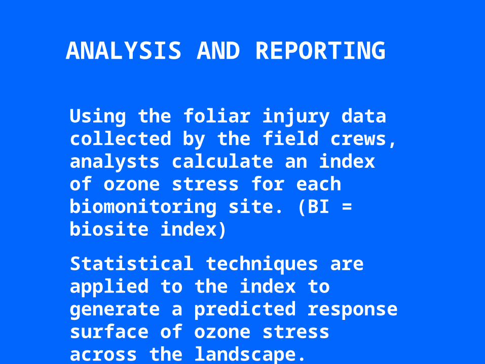
ANALYSIS AND REPORTING
Using the foliar injury data collected by the field crews, analysts calculate an index of ozone stress for each biomonitoring site. (BI = biosite index)
Statistical techniques are applied to the index to generate a predicted response surface of ozone stress across the landscape.
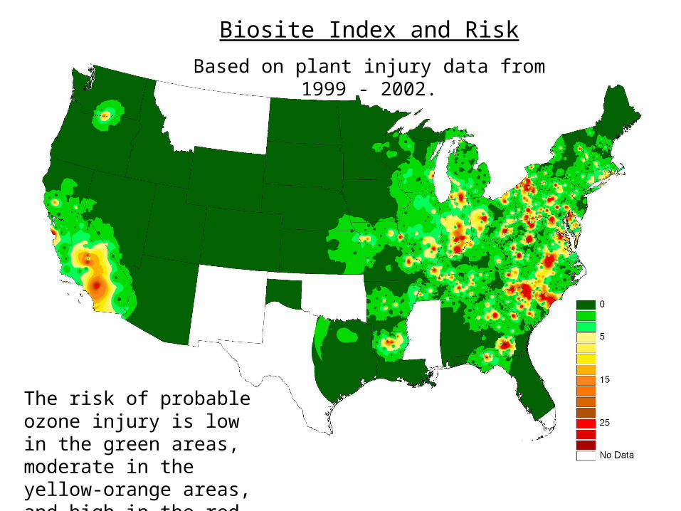
The risk of probable ozone injury is low in the green areas, moderate in the yellow-orange areas, and high in the red areas.
Biosite Index and Risk
Based on plant injury data from 1999 - 2002.
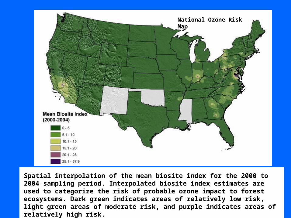
Spatial interpolation of the mean biosite index for the 2000 to 2004 sampling period. Interpolated biosite index estimates are used to categorize the risk of probable ozone impact to forest ecosystems. Dark green indicates areas of relatively low risk, light green areas of moderate risk, and purple indicates areas of relatively high risk. Areas in white are not sampled.
National Ozone Risk Map
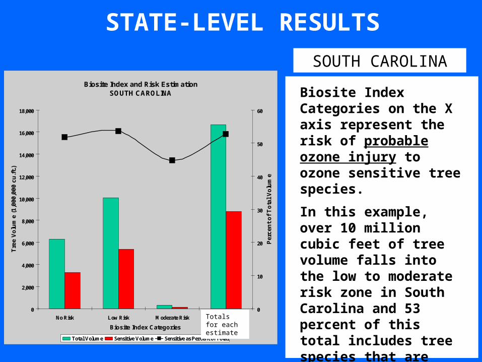
Biosite Index and Risk EstimationSOUTH CAROLINA
0
2,000
4,000
6,000
8,000
10,000
12,000
14,000
16,000
18,000
No Risk Low Risk Moderate Risk High Risk
Biosite Index Categories
Tre
e V
olu
me
(1,0
00,0
00 c
u.f
t.)
0
10
20
30
40
50
60
Per
cen
t o
f T
ota
l V
olu
me
Total Volume Sensitive Volume Sensitive as Percent of Total
Biosite Index Categories on the X axis represent the risk of probable ozone injury to ozone sensitive tree species.
In this example, over 10 million cubic feet of tree volume falls into the low to moderate risk zone in South Carolina and 53 percent of this total includes tree species that are ozone sensitive.
However, low foliar injury scores coupled with below average rainfall indicate low O3 impact.
STATE-LEVEL RESULTS
Totals for each estimate
SOUTH CAROLINA
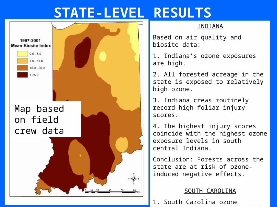
STATE-LEVEL RESULTSINDIANA
Based on air quality and biosite data:
1. Indiana’s ozone exposures are high.
2. All forested acreage in the state is exposed to relatively high ozone.
3. Indiana crews routinely record high foliar injury scores.
4. The highest injury scores coincide with the highest ozone exposure levels in south central Indiana.
Conclusion: Forests across the state are at risk of ozone-induced negative effects.
SOUTH CAROLINA
1. South Carolina ozone exposures are moderate to high.
2. Low injury scores associated with several years of below average rainfall indicate low risk of ozone impacts to South Carolina forests.
Map based on field crew data

EPA air quality data from physical air samplers
FIA air quality data from biomonitoring plots
Which map is better?Because the FIA Biosite Index is derived from plant response data, it has biological relevance.
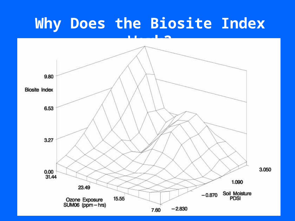
Why Does the Biosite Index Work?
O3
= Pa
thog
en
Tota
l of c
once
ntra
tion
and
dura
tion
of ex
posu
re
Environment
Total of conditions favoring ozone flux
Host PlantTotal of conditions favoring susceptibility
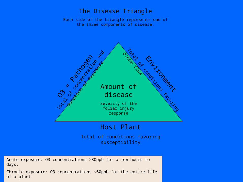
Amount of disease
Severity of the foliar injury response
The Disease TriangleEach side of the triangle represents one of the
three components of disease.
Acute exposure: O3 concentrations >80ppb for a few hours to days.
Chronic exposure: O3 concentrations <60ppb for the entire life of a plant.
Both acute and chronic exposures cause foliar injury and other adverse affects.
O3
= Pa
thog
en
Tota
l of c
once
ntra
tion
and
dura
tion
of ex
posu
re
Environment
Total of conditions favoring ozone flux
Host PlantTotal of conditions favoring susceptibility
Amount of disease
Severity of the foliar injury response
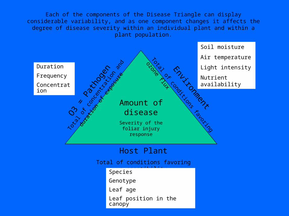
Species
Genotype
Leaf age
Leaf position in the canopy
Soil moisture
Air temperature
Light intensity
Nutrient availability
Each of the components of the Disease Triangle can display considerable variability, and as one component changes it affects the degree of disease severity
within an individual plant and within a plant population.
Duration
Frequency
Concentration
O3
= Pa
thog
en
Tota
l of c
once
ntra
tion
and
dura
tion
of ex
posu
re
Environment
Total of conditions favoring ozone flux
Host PlantTotal of conditions favoring susceptibility
Amount of
disease
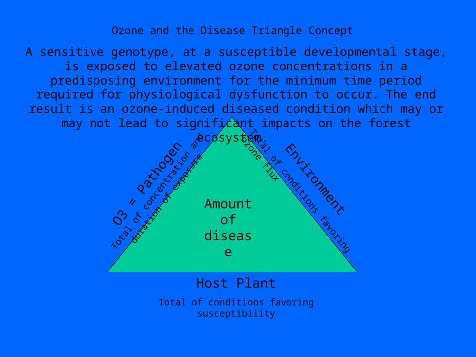
Ozone and the Disease Triangle Concept
A sensitive genotype, at a susceptible developmental stage, is exposed to elevated ozone concentrations in a predisposing environment for the minimum time period required for
physiological dysfunction to occur. The end result is an ozone-induced diseased condition which may or may not lead to significant impacts on the forest ecosystem.
THE BIOINDICATOR RESPONSE
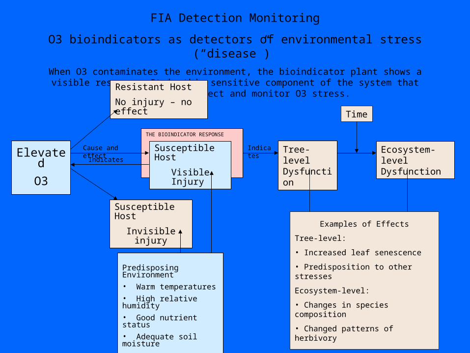
FIA Detection Monitoring
O3 bioindicators as detectors of environmental stress (“disease”)
When O3 contaminates the environment, the bioindicator plant shows a visible response. It is this sensitive component of the system that allows us to detect and monitor O3 stress.
Elevated
O3
Resistant Host
No injury – no effect
Susceptible Host
Visible Injury
Susceptible Host
Invisible injury
Cause and effect
Predisposing Environment
• Warm temperatures
• High relative humidity
• Good nutrient status
• Adequate soil moisture
Tree-level Dysfunction
Ecosystem-level Dysfunction
Time
Indicates
Indicates
Examples of Effects
Tree-level:
• Increased leaf senescence
• Predisposition to other stresses
Ecosystem-level:
• Changes in species composition
• Changed patterns of herbivory

15 minute BREAK
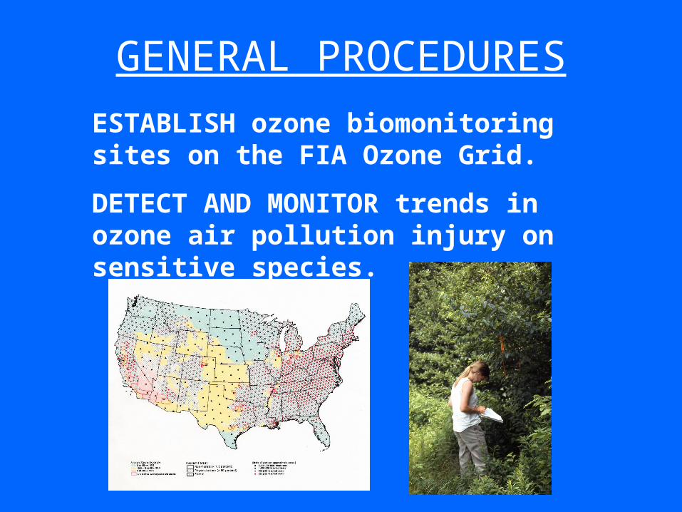
GENERAL PROCEDURES
ESTABLISH ozone biomonitoring sites on the FIA Ozone Grid.
DETECT AND MONITOR trends in ozone air pollution injury on sensitive species.

Objective: To select and map a high quality ozone biomonitoring site within each polygon on the FIA ozone grid.
SITE SELECTION
Rhode Island
Ozone Hexagon Number = the 7-digit number that identifies each polygon on the grid.
2008 FIA North - data collection software:
Ozone Hexagon Number = Field ID (F_ID)
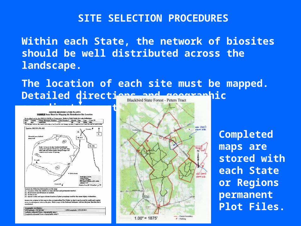
Within each State, the network of biosites should be well distributed across the landscape.
The location of each site must be mapped. Detailed directions and geographic coordinates must be documented.
SITE SELECTION PROCEDURES
Completed maps are stored with each State or Regions permanent Plot Files.
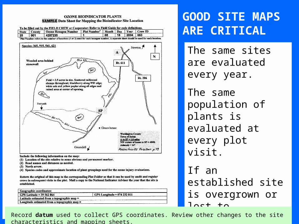
GOOD SITE MAPS ARE CRITICAL
The same sites are evaluated every year.
The same population of plants is evaluated at every plot visit.
If an established site is overgrown or lost to development, select a REPLACEMENT SITE and draw a new map.
Add new or missing information to old maps.
Record datum used to collect GPS coordinates. Review other changes to the site characteristics and mapping sheets.
WHAT’S ON THE MAP?
1. Location of the site relative to an obvious and permanent marker.
2. Road names and distances
3. North arrow
4. Species codes and approximate location of plant groupings
5. Starting point for ozone evaluations
6. Location and distance to at least 2 major roads
7. Distance and direction to 2 major towns
8. Gazetteer reference page if available
9. Point where GPS readings were taken. (record DATUM used)
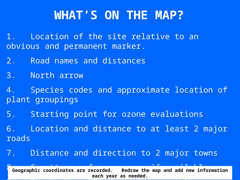
Geographic coordinates are recorded. Redraw the map and add new information each year as needed.
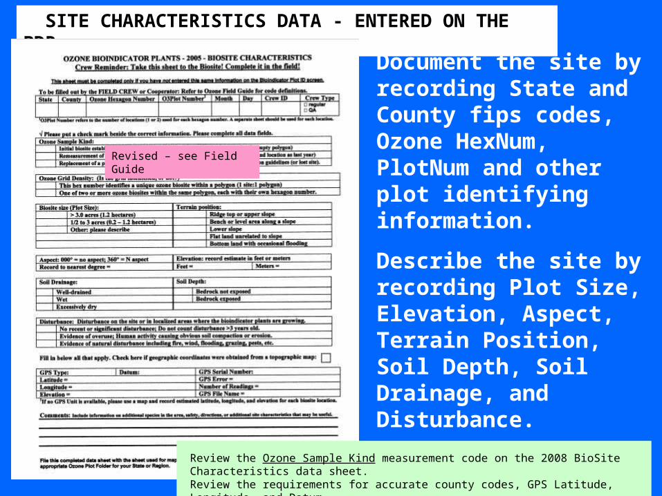
Document the site by recording State and County fips codes, Ozone HexNum, PlotNum and other plot identifying information.
Describe the site by recording Plot Size, Elevation, Aspect, Terrain Position, Soil Depth, Soil Drainage, and Disturbance.
Comment on safety or other useful information as needed.
SITE CHARACTERISTICS DATA - ENTERED ON THE PDR
Review the Ozone Sample Kind measurement code on the 2008 BioSite Characteristics data sheet. Review the requirements for accurate county codes, GPS Latitude, Longitude, and Datum.
Revised – see Field Guide
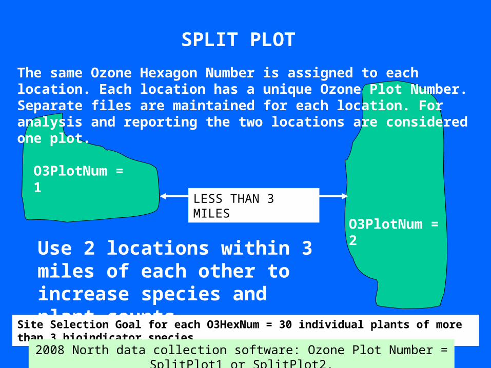
SPLIT PLOT
LESS THAN 3 MILES
O3PlotNum = 1
O3PlotNum = 2
Use 2 locations within 3 miles of each other to increase species and plant counts.
Site Selection Goal for each O3HexNum = 30 individual plants of more than 3 bioindicator species
The same Ozone Hexagon Number is assigned to each location. Each location has a unique Ozone Plot Number. Separate files are maintained for each location. For analysis and reporting the two locations are considered one plot.
2008 North data collection software: Ozone Plot Number = SplitPlot1 or SplitPlot2.
What Makes a Good Biomonitoring Site?
1. Easy and Safe Access
2. Wide Open Area Providing Good Air Mixing
Open areas must be greater than 1 acre.
The best sites are larger than 3 acres.
3. High Numbers of Species and Plant Counts
Each site should have at least 3 species.
The best sites have 5 species
Use split-plots to increase species and plant counts.
Continued...
What Makes a Good Biomonitoring Site?
4. Low Drought Potential
Avoid obviously dry or shallow soils.
5. Reasonable Fertility
Based on your best judgement.
6. No Obvious or Significant Disturbance
Natural disturbances that would limit site quality are fire and grazing.
Human activities that cause obvious soil compaction, erosion, or contamination by pesticides make a site unacceptable.
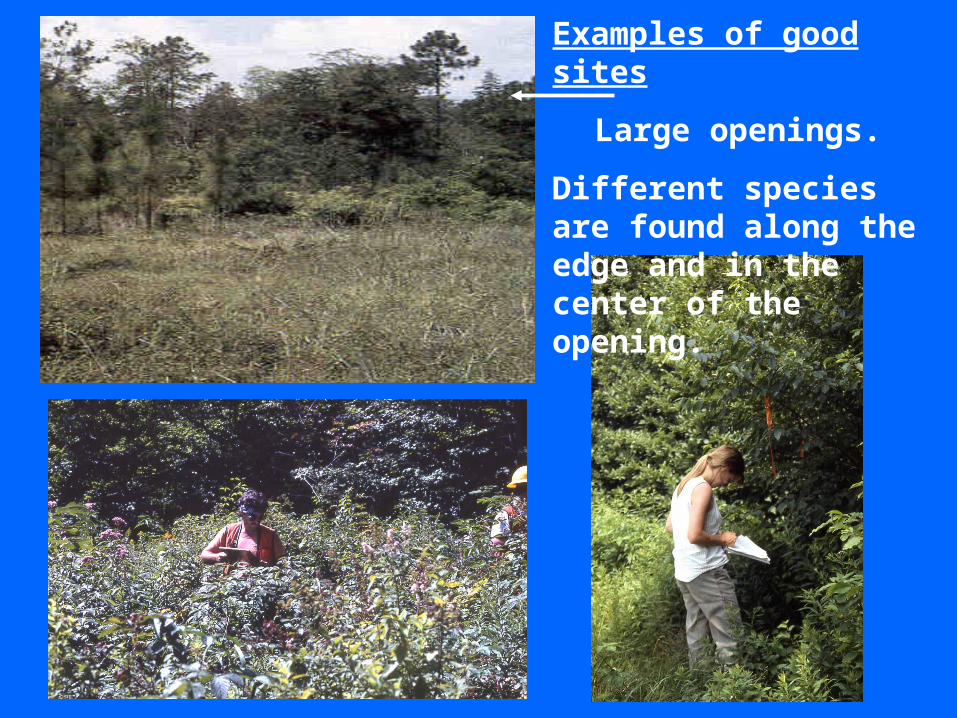
Examples of good sites
Large openings.
Different species are found along the edge and in the center of the opening.
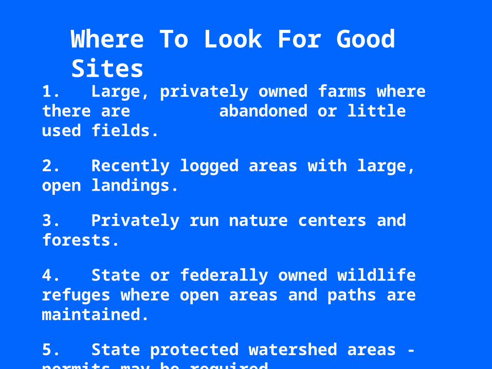
Where To Look For Good Sites
1. Large, privately owned farms where there are abandoned or little used fields.
2. Recently logged areas with large, open landings.
3. Privately run nature centers and forests.
4. State or federally owned wildlife refuges where open areas and paths are maintained.
5. State protected watershed areas - permits may be required.
6. State forests and parks with remote camping areas.
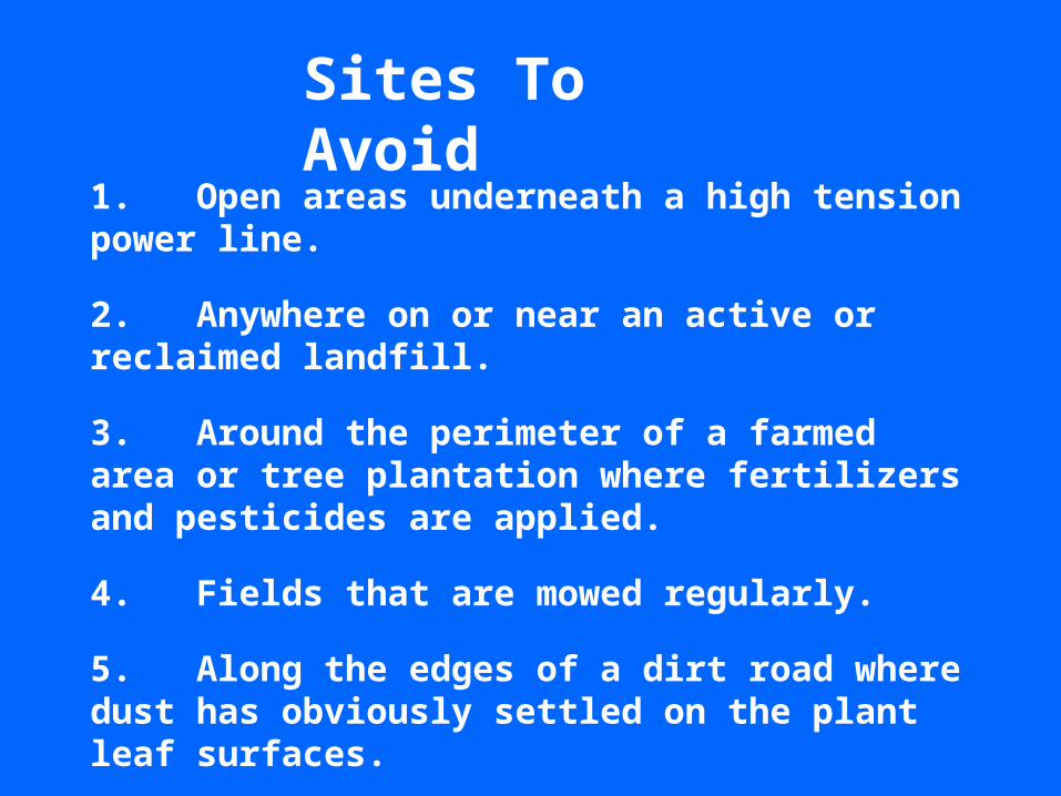
Sites To Avoid
1. Open areas underneath a high tension power line.
2. Anywhere on or near an active or reclaimed landfill.
3. Around the perimeter of a farmed area or tree plantation where fertilizers and pesticides are applied.
4. Fields that are mowed regularly.
5. Along the edges of a dirt road where dust has obviously settled on the plant leaf surfaces.
6. Any area obviously stressed by people traffic.
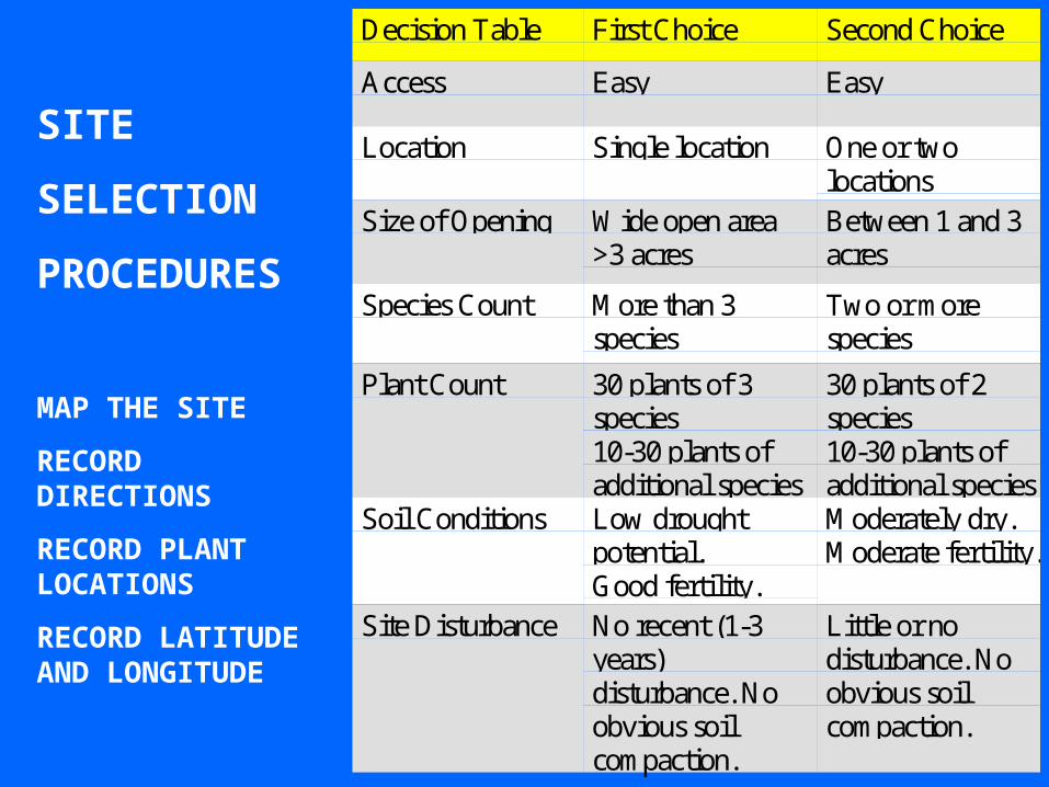
SITE
SELECTION
PROCEDURES
MAP THE SITE
RECORD DIRECTIONS
RECORD PLANT LOCATIONS
RECORD LATITUDE AND LONGITUDE
Decision Table First Choice Second Choice
Access Easy Easy
Location Single location One or twolocations
Size of Opening Wide open area>3 acres
Between 1 and 3acres
Species Count More than 3species
Two or morespecies
Plant Count 30 plants of 3species10-30 plants ofadditional species
30 plants of 2species10-30 plants ofadditional species
Soil Conditions Low droughtpotential.Good fertility.
Moderately dry.Moderate fertility.
Site Disturbance No recent (1-3years)disturbance. Noobvious soilcompaction.
Little or nodisturbance. Noobvious soilcompaction.
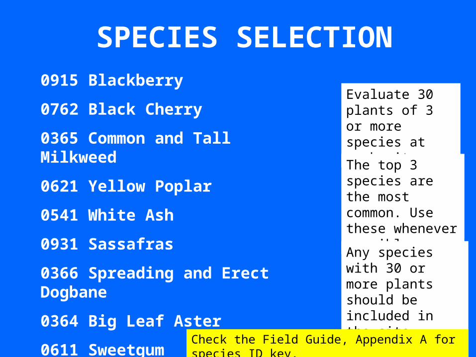
SPECIES SELECTION0915 Blackberry
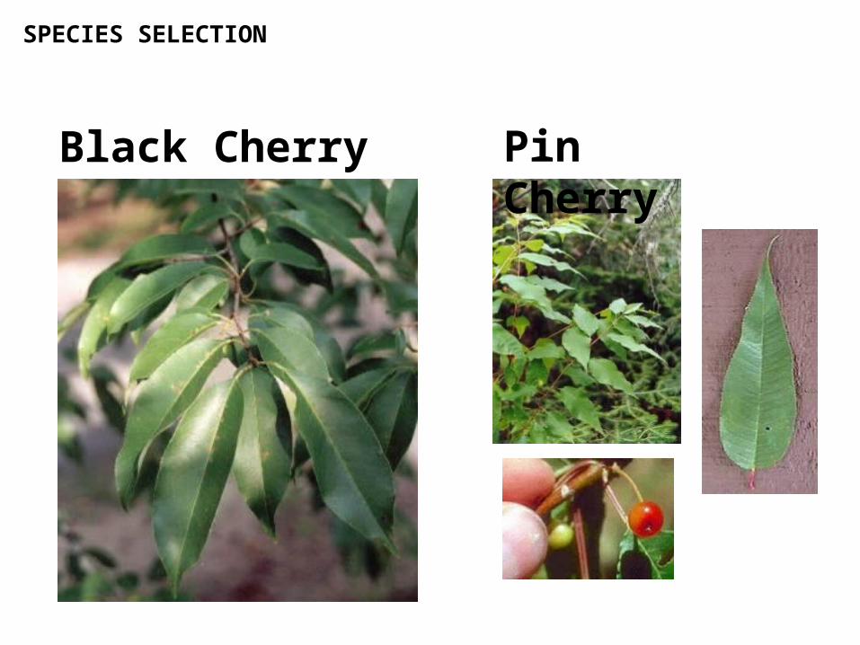
0762 Black Cherry
0365 Common and Tall Milkweed
0621 Yellow Poplar
0541 White Ash
0931 Sassafras
0366 Spreading and Erect Dogbane
0364 Big Leaf Aster
0611 Sweetgum
0761 Pin Cherry
Evaluate 30 plants of 3 or more species at each site.
The top 3 species are the most common. Use these whenever possible.
Any species with 30 or more plants should be included in the site evaluation.
Check the Field Guide, Appendix A for species ID key.
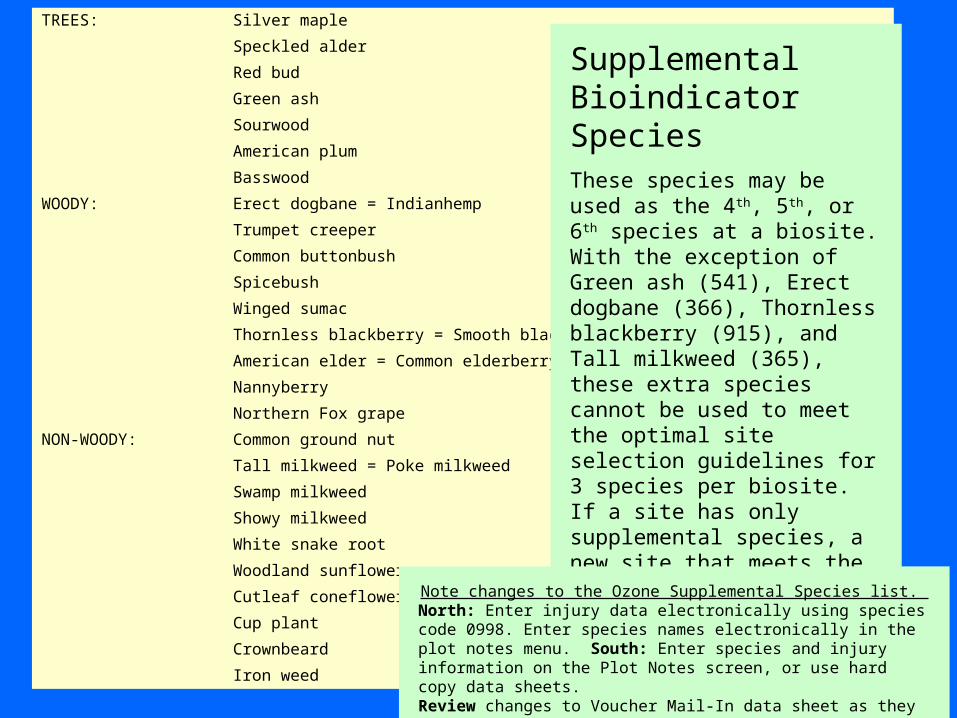
TREES: Silver maple
Speckled alder
Red bud
Green ash
Sourwood
American plum
Basswood
WOODY: Erect dogbane = Indianhemp
Trumpet creeper
Common buttonbush
Spicebush
Winged sumac
Thornless blackberry = Smooth blackberry
American elder = Common elderberry
Nannyberry
Northern Fox grape
NON-WOODY: Common ground nut
Tall milkweed = Poke milkweed
Swamp milkweed
Showy milkweed
White snake root
Woodland sunflower
Cutleaf coneflower
Cup plant
Crownbeard
Iron weed
Supplemental Bioindicator SpeciesThese species may be used as the 4th, 5th, or 6th species at a biosite. With the exception of Green ash (541), Erect dogbane (366), Thornless blackberry (915), and Tall milkweed (365), these extra species cannot be used to meet the optimal site selection guidelines for 3 species per biosite. If a site has only supplemental species, a new site that meets the biosite selection guidelines must be located and mapped.
See handouts for species ID information.
Note changes to the Ozone Supplemental Species list. North: Enter injury data electronically using species code 0998. Enter species names electronically in the plot notes menu. South: Enter species and injury information on the Plot Notes screen, or use hard copy data sheets. Review changes to Voucher Mail-In data sheet as they relate to the collection of leaf samples for supplemental or unknown species .
SPECIES SELECTION
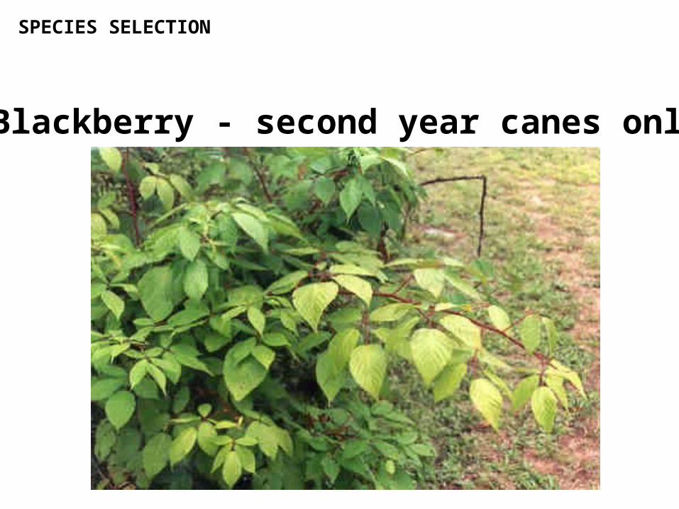
Blackberry - second year canes only
SPECIES SELECTION
Black Cherry Pin Cherry
SPECIES SELECTION
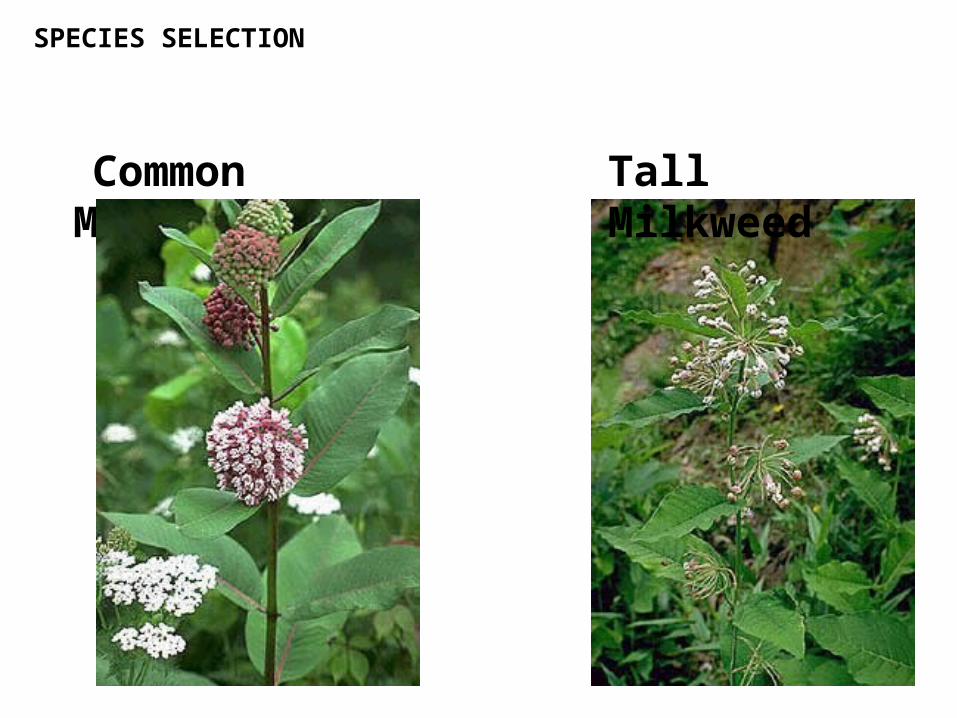
Common Milkweed Tall Milkweed

SPECIES SELECTION
Yellow Poplar
SPECIES SELECTION
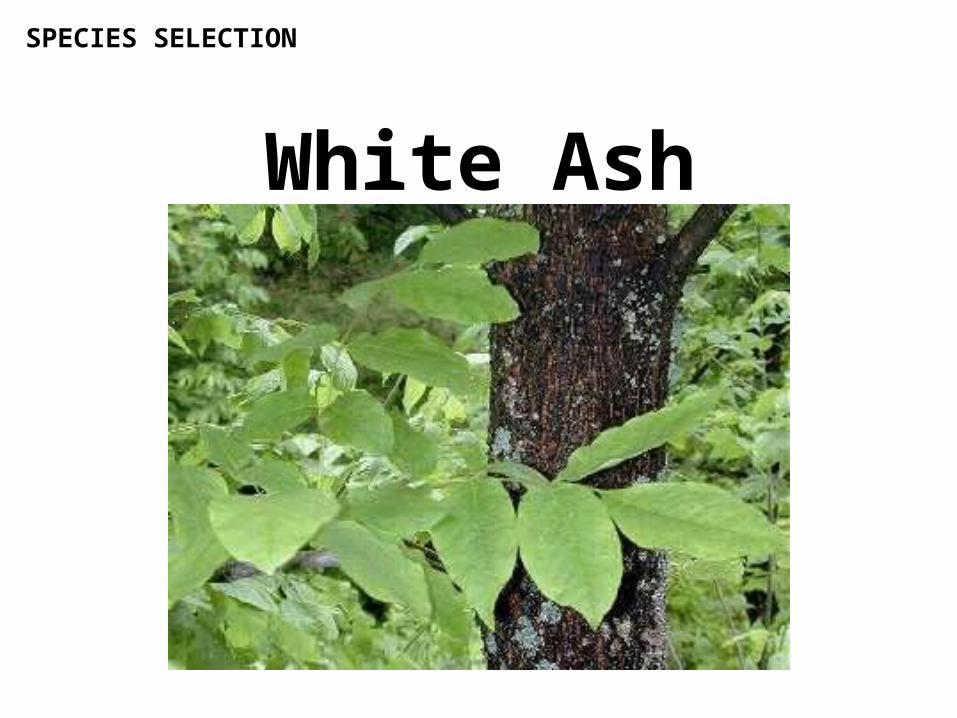
White Ash
SPECIES SELECTION
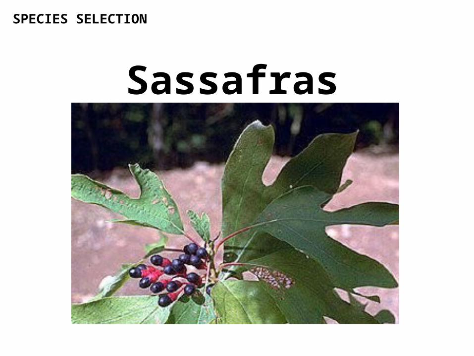
Sassafras
SPECIES SELECTION
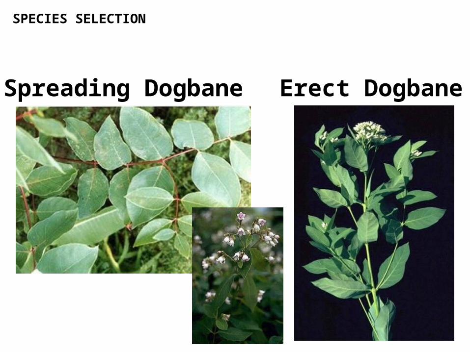
Spreading Dogbane Erect Dogbane
SPECIES SELECTION
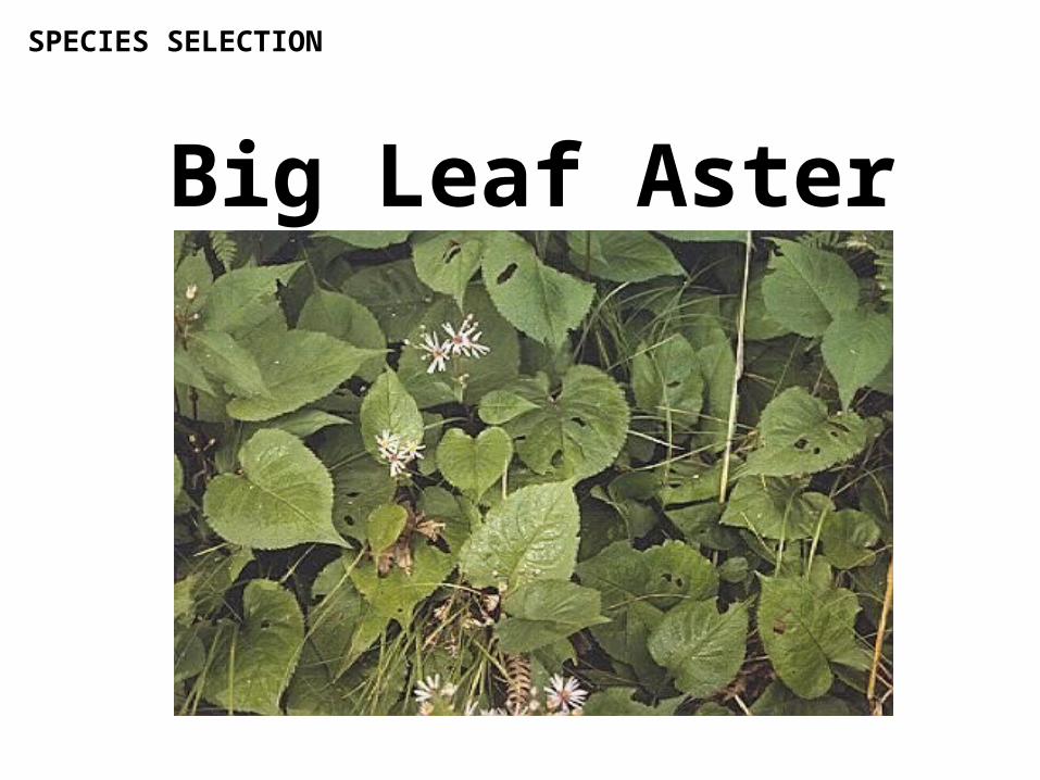
Big Leaf Aster
SPECIES SELECTION
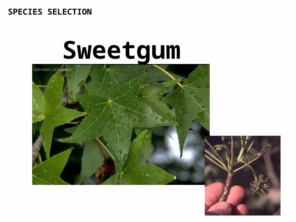
Sweetgum
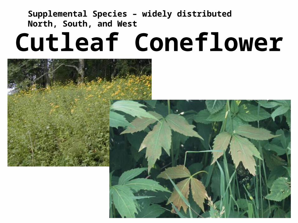
Supplemental Species – widely distributed North, South, and West
Cutleaf Coneflower
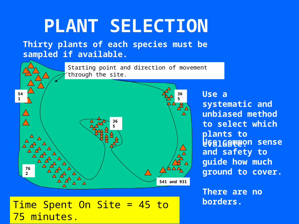
PLANT SELECTION
Starting point and direction of movement through the site.
762
365
541 and 931
541
Time Spent On Site = 45 to 75 minutes.
Use a systematic and unbiased method to select which plants to evaluate.
Use common sense and safety to guide how much ground to cover.
There are no borders.
365
Thirty plants of each species must be sampled if available.
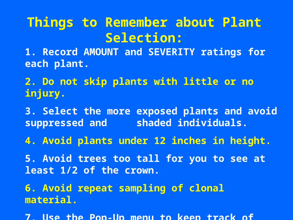
Things to Remember about Plant Selection:
1. Record AMOUNT and SEVERITY ratings for each plant.
2. Do not skip plants with little or no injury.
3. Select the more exposed plants and avoid suppressed and shaded individuals.
4. Avoid plants under 12 inches in height.
5. Avoid trees too tall for you to see at least 1/2 of the crown.
6. Avoid repeat sampling of clonal material.
7. Use the Pop-Up menu to keep track of plant counts.
8. ZERO values (no injury) are important!
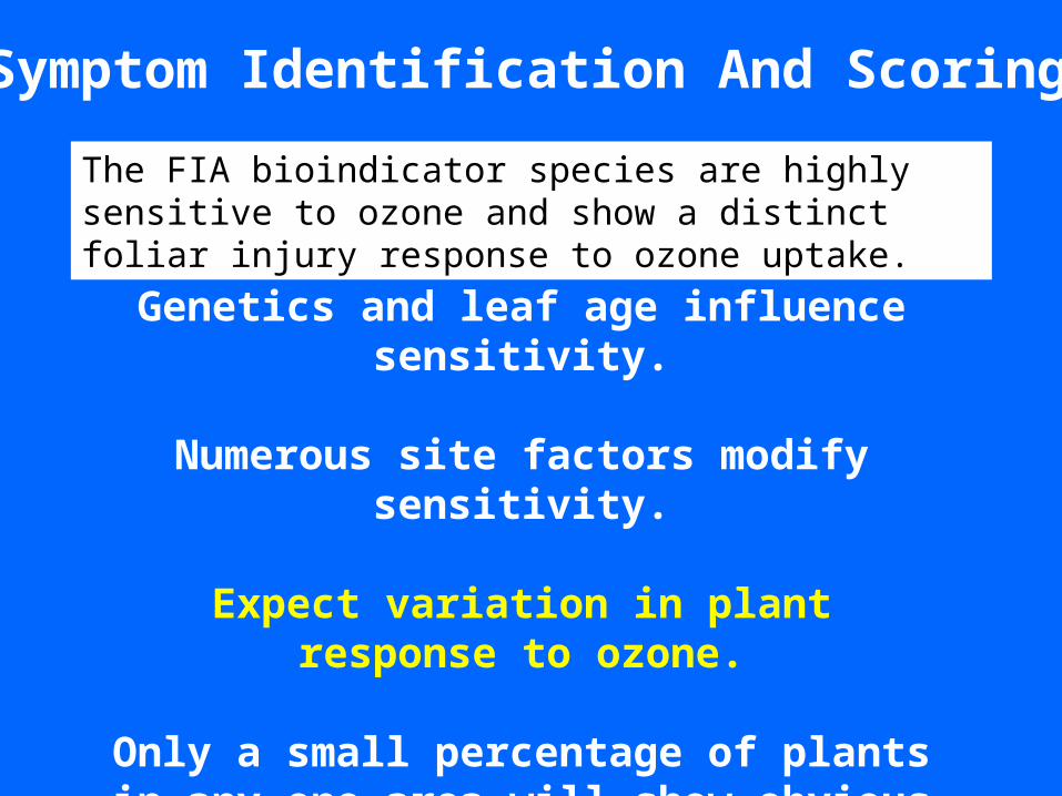
Symptom Identification And Scoring
The FIA bioindicator species are highly sensitive to ozone and show a distinct foliar injury response to ozone uptake.
Genetics and leaf age influence sensitivity.
Numerous site factors modify sensitivity.
Expect variation in plant response to ozone.
Only a small percentage of plants in any one area will show obvious symptoms.
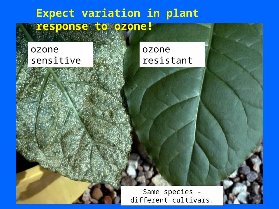
Expect variation in plant response to ozone!
Same species - different cultivars.
ozone sensitive ozone resistant
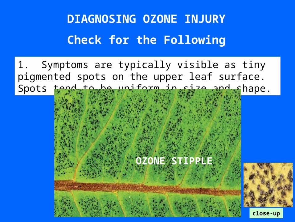
DIAGNOSING OZONE INJURY
Check for the Following
1. Symptoms are typically visible as tiny pigmented spots on the upper leaf surface. Spots tend to be uniform in size and shape.
OZONE STIPPLE
close-up
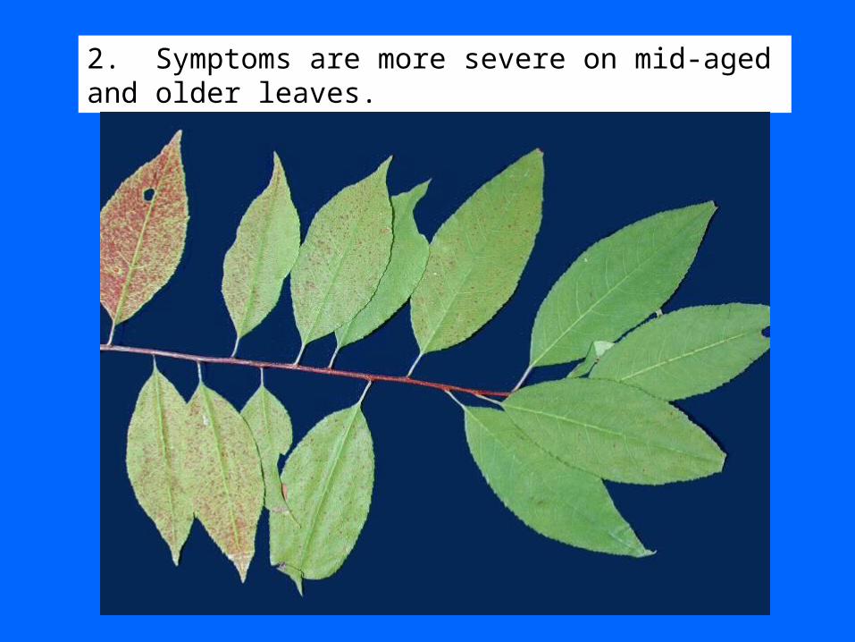
2. Symptoms are more severe on mid-aged and older leaves.
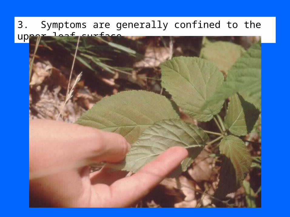
3. Symptoms are generally confined to the upper leaf surface.
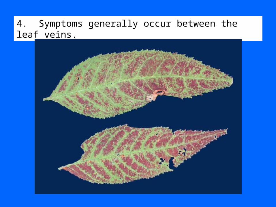
4. Symptoms generally occur between the leaf veins.
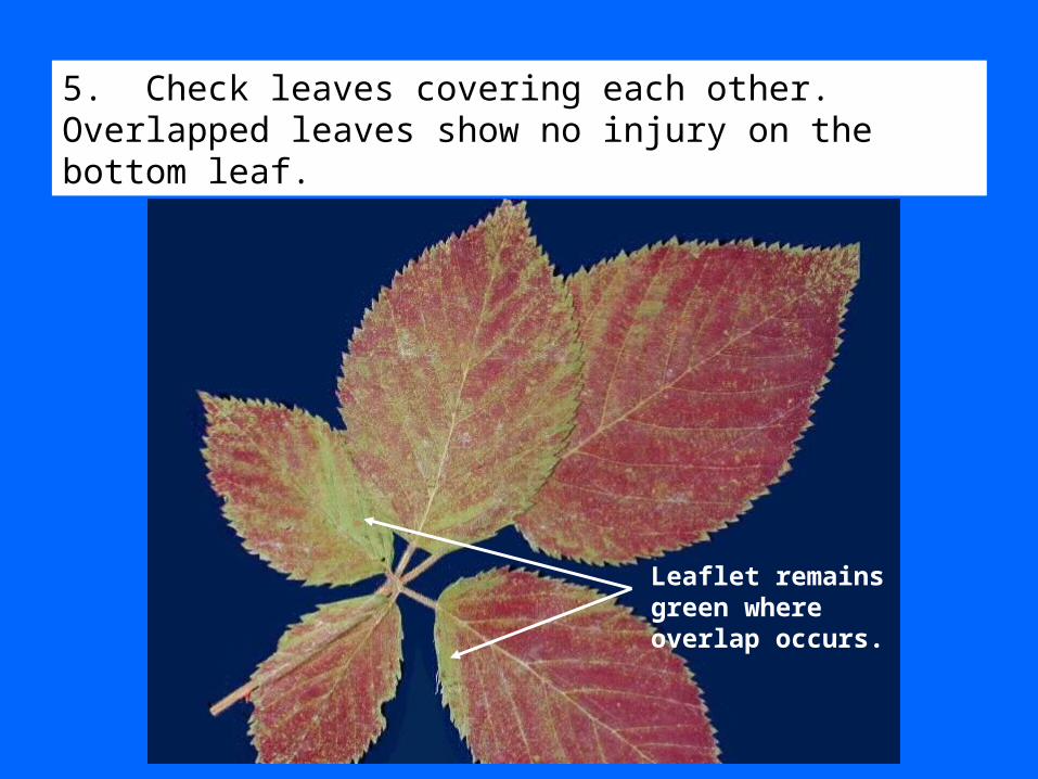
5. Check leaves covering each other. Overlapped leaves show no injury on the bottom leaf.
Leaflet remains green where overlap occurs.
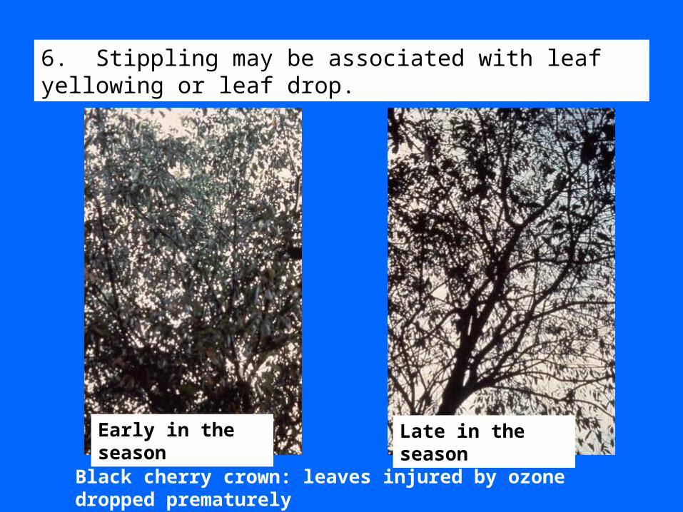
6. Stippling may be associated with leaf yellowing or leaf drop.
Early in the season Late in the season
Black cherry crown: leaves injured by ozone dropped prematurely
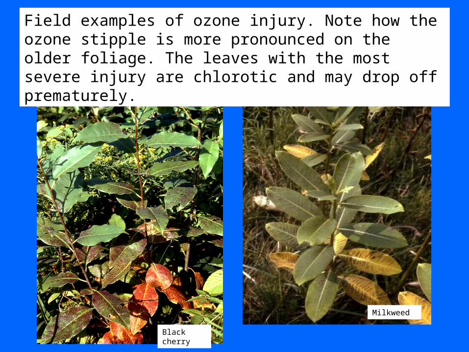
Field examples of ozone injury. Note how the ozone stipple is more pronounced on the older foliage. The leaves with the most severe injury are chlorotic and may drop off prematurely.
Black cherry
Milkweed
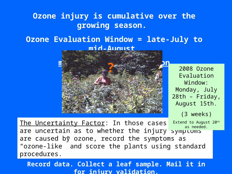
Ozone injury is cumulative over the growing season.
Ozone Evaluation Window = late-July to mid-August
maximize ozone detection
Don’t Waste Time!
Record data. Collect a leaf sample. Mail it in for injury validation.
?
The Uncertainty Factor: In those cases where you are uncertain as to whether the injury symptoms are caused by ozone, record the symptoms as “ozone-like” and score the plants using standard procedures.
2008 Ozone Evaluation Window: Monday, July 28th – Friday, August 15th.
(3 weeks)Extend to August 20th as needed.
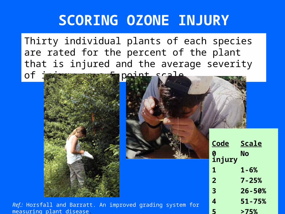
SCORING OZONE INJURYThirty individual plants of each species are rated for the percent of the plant that is injured and the average severity of injury on a 5-point scale.
Code Scale
0 No injury
1 1-6%
2 7-25%
3 26-50%
4 51-75%
5 >75%Ref.: Horsfall and Barratt. An improved grading system for measuring plant disease.
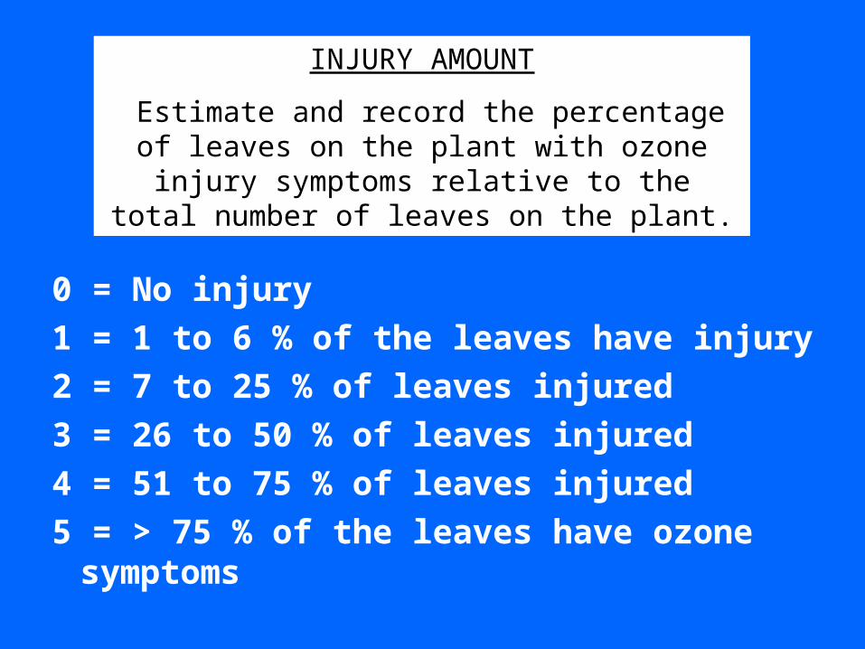
INJURY AMOUNT
Estimate and record the percentage of leaves on the plant with ozone injury symptoms relative to the total
number of leaves on the plant.
0 = No injury
1 = 1 to 6 % of the leaves have injury
2 = 7 to 25 % of leaves injured
3 = 26 to 50 % of leaves injured
4 = 51 to 75 % of leaves injured
5 = > 75 % of the leaves have ozone symptoms
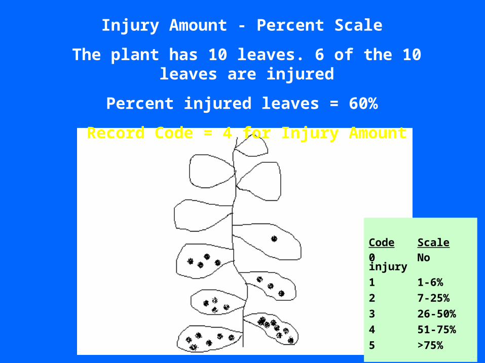
Injury Amount - Percent Scale
The plant has 10 leaves. 6 of the 10 leaves are injured
Percent injured leaves = 60%
Record Code = 4 for Injury Amount
Code Scale
0 No injury
1 1-6%
2 7-25%
3 26-50%
4 51-75%
5 >75%
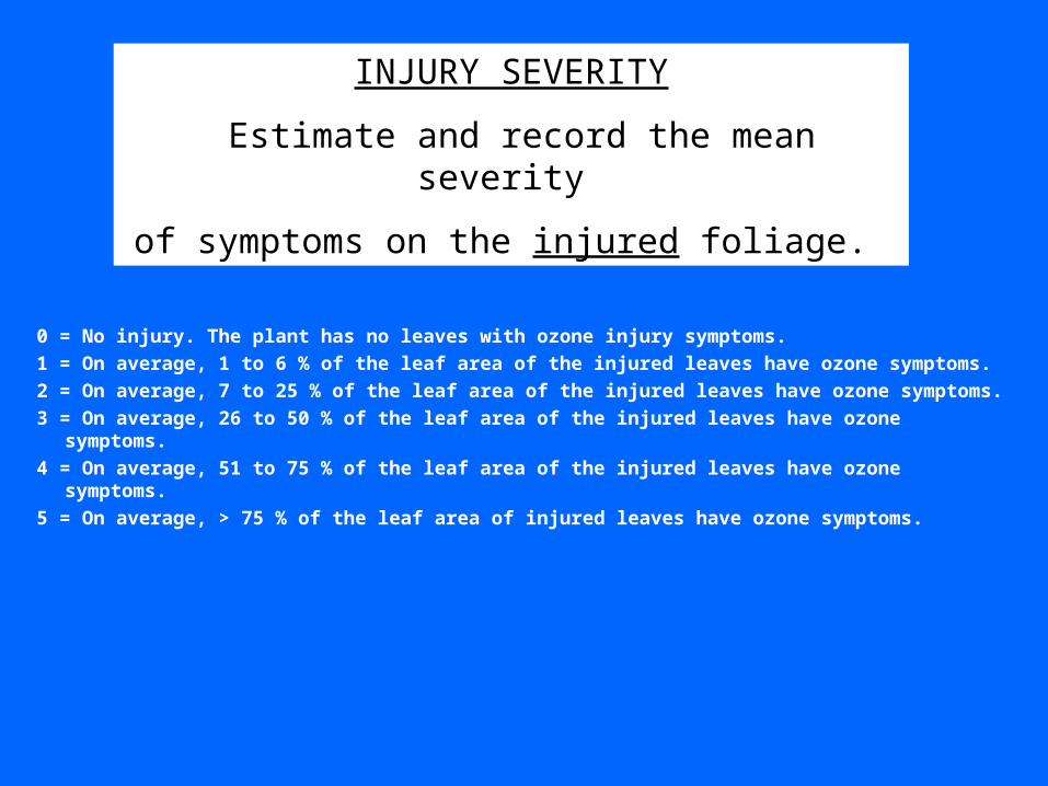
INJURY SEVERITY
Estimate and record the mean severity
of symptoms on the injured foliage.
0 = No injury. The plant has no leaves with ozone injury symptoms.
1 = On average, 1 to 6 % of the leaf area of the injured leaves have ozone symptoms.
2 = On average, 7 to 25 % of the leaf area of the injured leaves have ozone symptoms.
3 = On average, 26 to 50 % of the leaf area of the injured leaves have ozone symptoms.
4 = On average, 51 to 75 % of the leaf area of the injured leaves have ozone symptoms.
5 = On average, > 75 % of the leaf area of injured leaves have ozone symptoms.
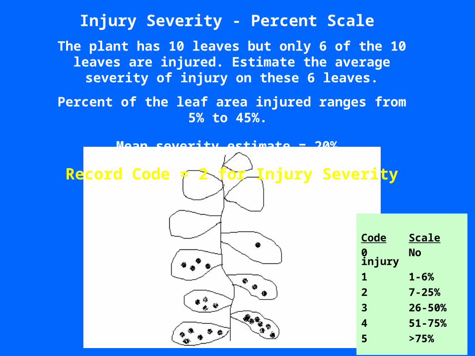
Injury Severity - Percent Scale
The plant has 10 leaves but only 6 of the 10 leaves are injured. Estimate the average severity of injury on these 6 leaves.
Percent of the leaf area injured ranges from 5% to 45%.
Mean severity estimate = 20%
Record Code = 2 for Injury Severity
Code Scale
0 No injury
1 1-6%
2 7-25%
3 26-50%
4 51-75%
5 >75%
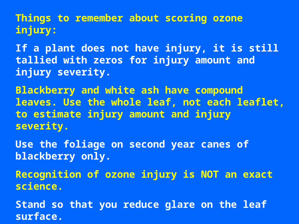
Things to remember about scoring ozone injury:
If a plant does not have injury, it is still tallied with zeros for injury amount and injury severity.
Blackberry and white ash have compound leaves. Use the whole leaf, not each leaflet, to estimate injury amount and injury severity.
Use the foliage on second year canes of blackberry only.
Recognition of ozone injury is NOT an exact science.
Stand so that you reduce glare on the leaf surface.
Long periods without rain will inhibit symptom development.
Do not take measurements in steady rain.
COMMUNICATE – use the plot notes menu and data sheet!
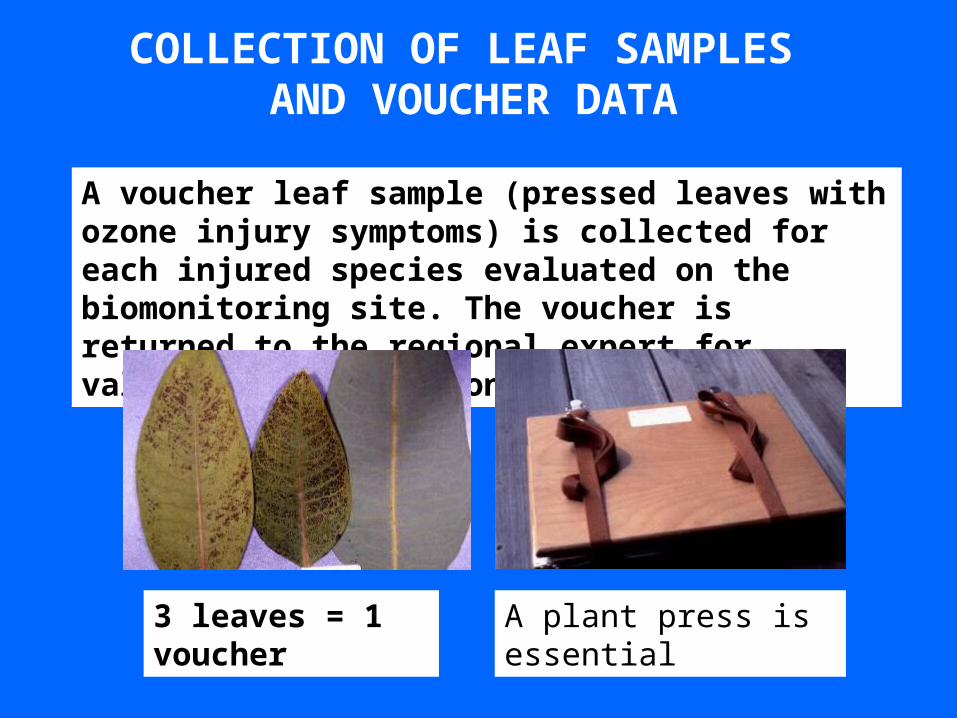
COLLECTION OF LEAF SAMPLES AND VOUCHER DATA
A voucher leaf sample (pressed leaves with ozone injury symptoms) is collected for each injured species evaluated on the biomonitoring site. The voucher is returned to the regional expert for validation of the ozone injury symptom.
3 leaves = 1 voucher A plant press is essential
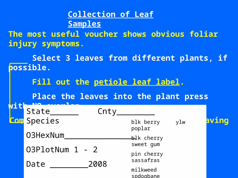
Collection of Leaf Samples
The most useful voucher shows obvious foliar injury symptoms.
Select 3 leaves from different plants, if possible.
Fill out the petiole leaf label.
Place the leaves into the plant press with NO overlap.
Complete the voucher data sheet before leaving the biosite.
State______ Cnty________ Species
O3HexNum_______________
O3PlotNum 1 - 2
Date ________2008
blk berry ylw poplar
blk cherry sweet gum
pin cherry sassafras
milkweed spdogbane
white ash blaster
State: 42 County: 13
O3HexNum: 4107814 O3PlotNum: 2
Date: 7/30/03 Species: 365
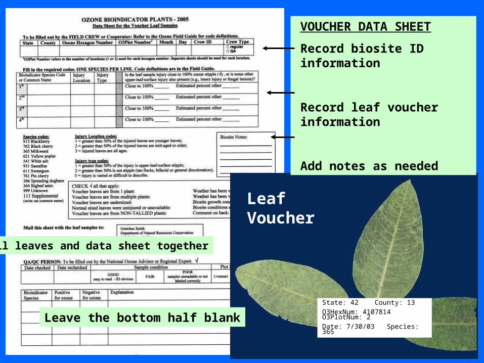
VOUCHER DATA SHEET
Record biosite ID information
Record leaf voucher information
Add notes as needed
Leaf Voucher
Leave the bottom half blank
Mail leaves and data sheet together
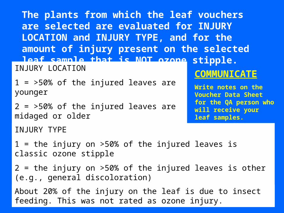
The plants from which the leaf vouchers are selected are evaluated for INJURY LOCATION and INJURY TYPE, and for the amount of injury present on the selected leaf sample that is NOT ozone stipple.
INJURY LOCATION
1 = >50% of the injured leaves are younger
2 = >50% of the injured leaves are midaged or older
3 = injured leaves are all ages
INJURY TYPE
1 = the injury on >50% of the injured leaves is classic ozone stipple
2 = the injury on >50% of the injured leaves is other (e.g., general discoloration)
3 = the injury is varied or, otherwise, difficult to describe
About 20% of the injury on the leaf is due to insect feeding. This was not rated as ozone injury.
COMMUNICATEWrite notes on the Voucher Data Sheet for the QA person who will receive your leaf samples.
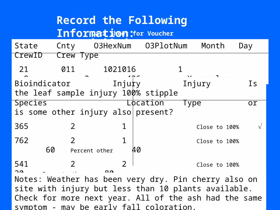
State Cnty O3HexNum O3PlotNum Month Day CrewID Crew Type
21 011 1021016 1 8 2 426 X regular
Record the Following Information:
Bioindicator Injury Injury Is the leaf sample injury 100% stippleSpecies Location Type or is some other injury also present?
365 2 1 Close to 100%
762 2 1 Close to 100% 60 Percent other 40
541 2 2 Close to 100% 20 Percent other 80
915 3 1 Close to 100%
Notes: Weather has been very dry. Pin cherry also on site with injury but less than 10 plants available. Check for more next year. All of the ash had the same symptom - may be early fall coloration.
Data Sheet for Voucher leaf Samples
Things to remember about leaf vouchers:
A voucher consists of THREE leaves.
Label the leaf voucher
Use the plant press or the leaf sample will be ruined
Species with compound leaves - send the whole leaf, not leaflets.
Complete the top half of the voucher data sheet
Do not tape, glue, or staple leaves to the data sheet.
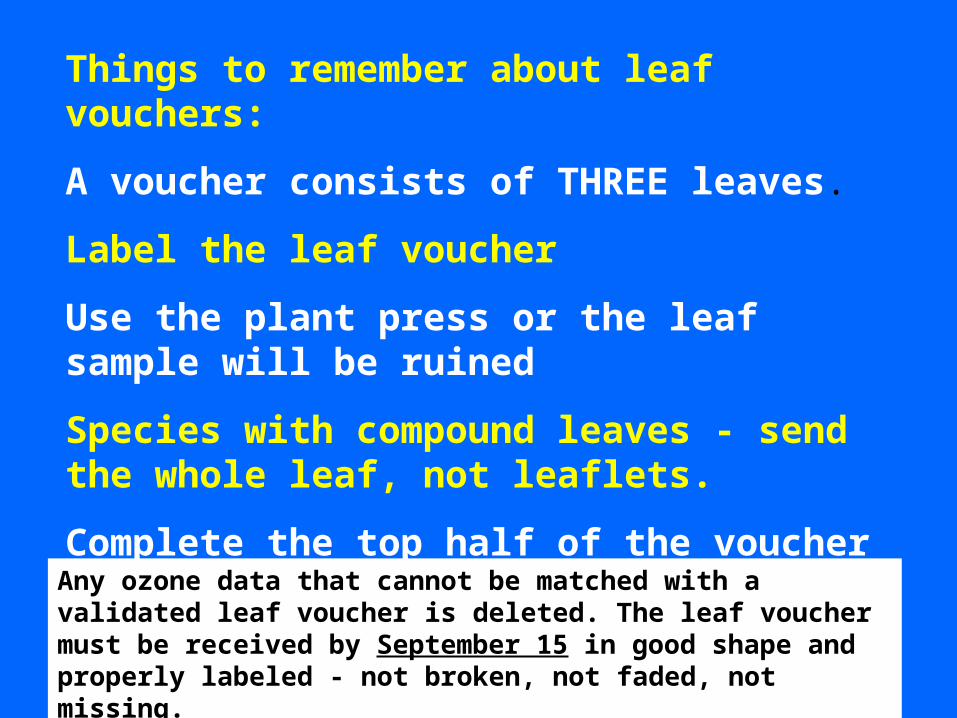
Any ozone data that cannot be matched with a validated leaf voucher is deleted. The leaf voucher must be received by September 15 in good shape and properly labeled - not broken, not faded, not missing.
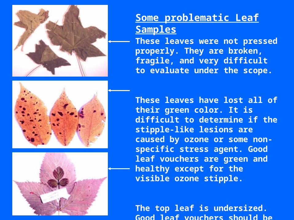
Some problematic Leaf Samples
These leaves were not pressed properly. They are broken, fragile, and very difficult to evaluate under the scope.
These leaves have lost all of their green color. It is difficult to determine if the stipple-like lesions are caused by ozone or some non-specific stress agent. Good leaf vouchers are green and healthy except for the visible ozone stipple.
The top leaf is undersized. Good leaf vouchers should be as close to normal leaf size as possible.
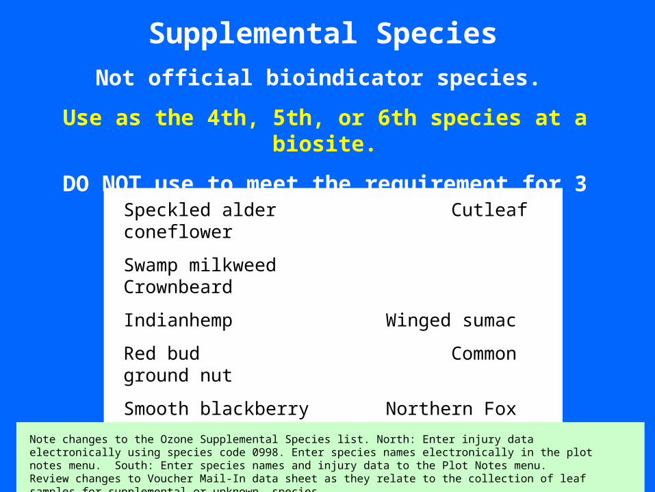
Supplemental Species
Not official bioindicator species.
Use as the 4th, 5th, or 6th species at a biosite.
DO NOT use to meet the requirement for 3 species per biosite.
Speckled alder Cutleaf coneflower
Swamp milkweed Crownbeard
Indianhemp Winged sumac
Red bud Common ground nut
Smooth blackberry Northern Fox grape
Common elderberry White snake root
Note changes to the Ozone Supplemental Species list. North: Enter injury data electronically using species code 0998. Enter species names electronically in the plot notes menu. South: Enter species names and injury data to the Plot Notes menu. Review changes to Voucher Mail-In data sheet as they relate to the collection of leaf samples for supplemental or unknown species.
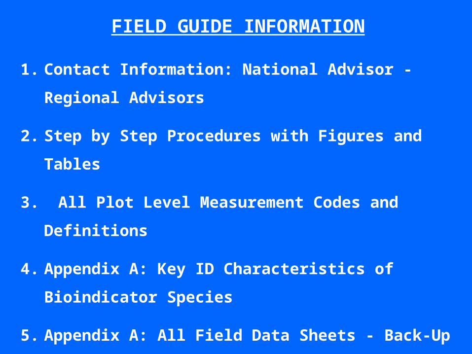
FIELD GUIDE INFORMATION
1. Contact Information: National Advisor - Regional Advisors
2. Step by Step Procedures with Figures and Tables
3. All Plot Level Measurement Codes and Definitions
4. Appendix A: Key ID Characteristics of Bioindicator Species
5. Appendix A: All Field Data Sheets - Back-Up
6. Appendix B: Detail on Handling Leaf Vouchers
7. Appendix C: Site Ranking and Biosite Selection
8. Appendix D: Supplemental Species List
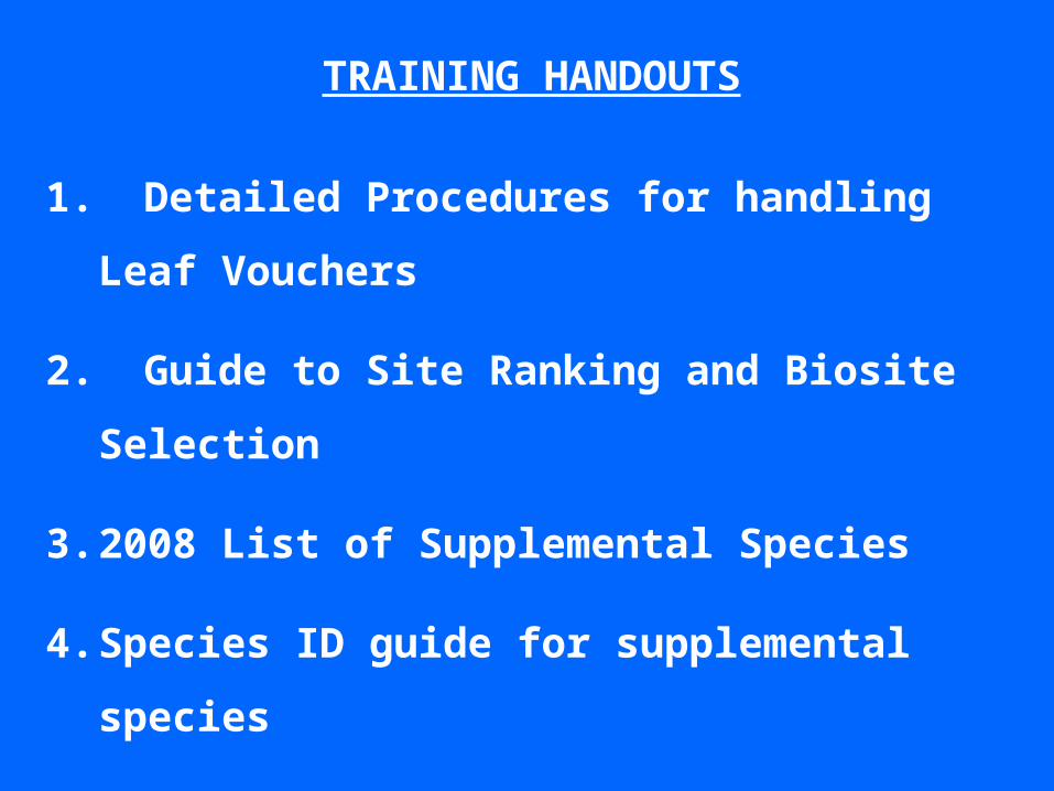
TRAINING HANDOUTS
1. Detailed Procedures for handling Leaf Vouchers
2. Guide to Site Ranking and Biosite Selection
3. 2008 List of Supplemental Species
4. Species ID guide for supplemental species
5. Field Data Sheets, mailing envelopes and labels
6. Notification of Data Collection outside the Window
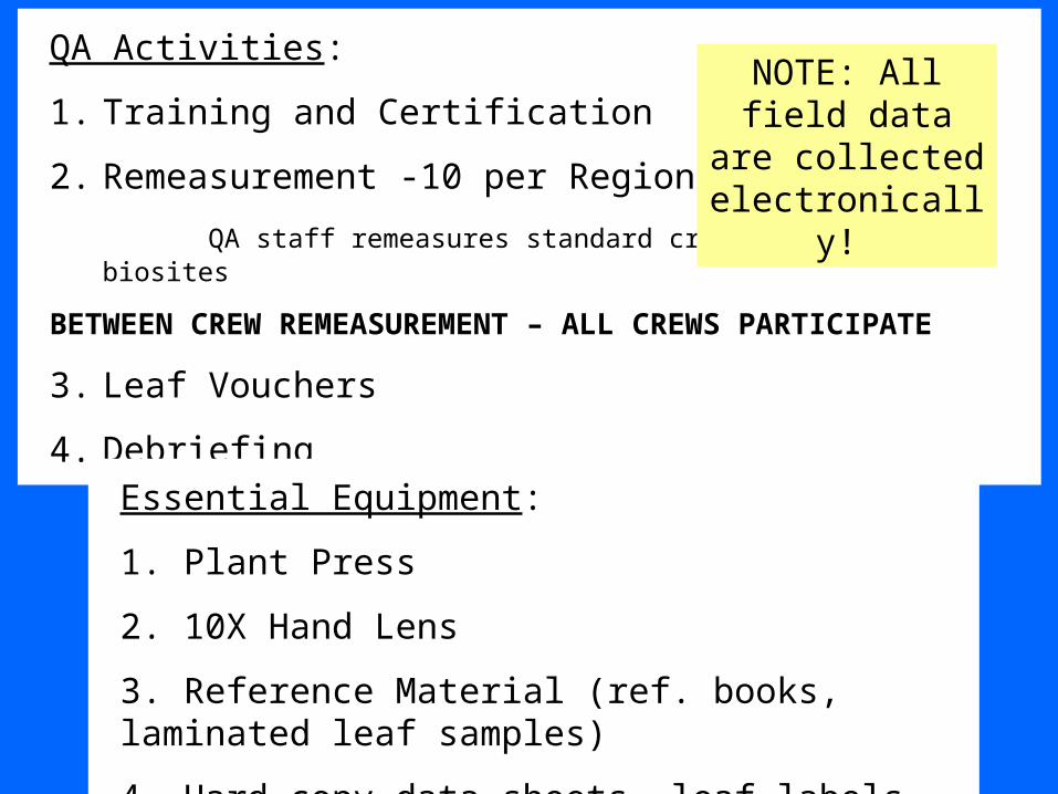
QA Activities:
1. Training and Certification
2. Remeasurement -10 per Region
QA staff remeasures standard crew – select biosites
BETWEEN CREW REMEASUREMENT – ALL CREWS PARTICIPATE
3. Leaf Vouchers
4. Debriefing
Essential Equipment:
1. Plant Press
2. 10X Hand Lens
3. Reference Material (ref. books, laminated leaf samples)
4. Hard copy data sheets, leaf labels, mailing envelopes
NOTE: All field data are collected electronically!
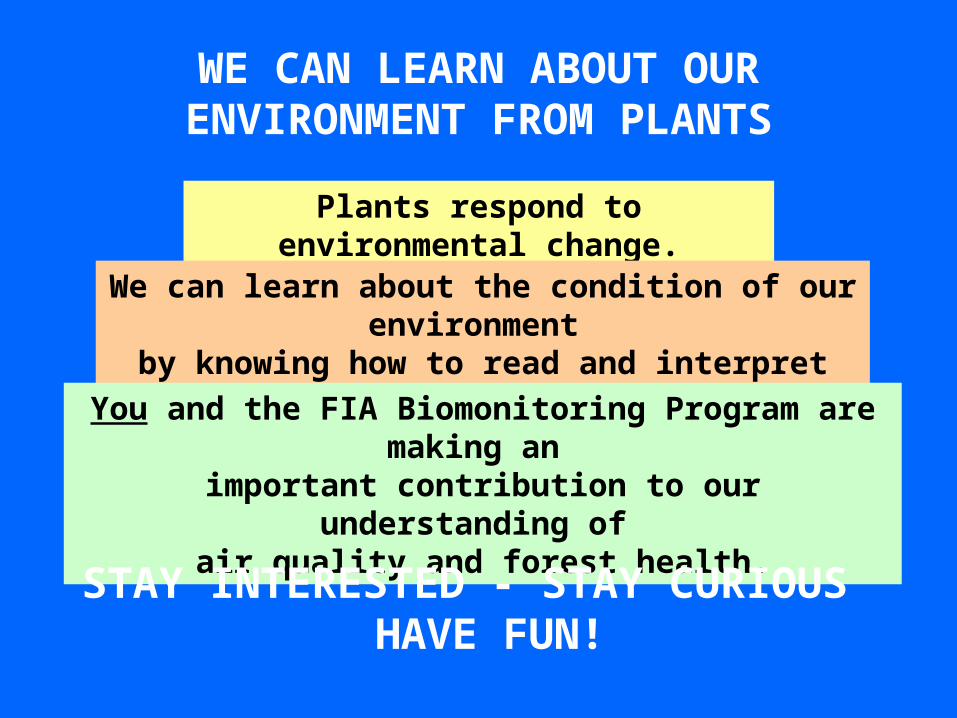
WE CAN LEARN ABOUT OUR ENVIRONMENT FROM PLANTS
Plants respond to environmental change.
We can learn about the condition of our environment by knowing how to read and interpret plant responses.
You and the FIA Biomonitoring Program are making an important contribution to our understanding of
air quality and forest health.
STAY INTERESTED - STAY CURIOUS HAVE FUN!
END
“To the philosopher, the physician, the meteorologist, and the chemist, there is perhaps no subject more attractive than that of ozone.”
Fox, C.B. 1873. Ozone and Antozone. J. & A. Churchell, London.