notes on atmospheric physics - imperialaczaja/pdf/notes.pdf · notes on atmospheric physics arnaud...
TRANSCRIPT
Notes on Atmospheric Physics
Arnaud Czaja1
Physics Department &Grantham Institute for Climate Change,
Imperial College, London.
May 5, 2017
1Contact details: Huxley Building, Room 726; email: [email protected] Hours: Thursdays, 11.30-12.30; Fridays, 1-2pm.

2
Contents
1 An overview of the atmosphere 11.1 Atmospheric composition . . . . . . . . . . . . . . . . . . . . . 21.2 Mass . . . . . . . . . . . . . . . . . . . . . . . . . . . . . . . . 4
1.2.1 Pressure as a measure of mass . . . . . . . . . . . . . . 41.2.2 Measures of water in air . . . . . . . . . . . . . . . . . 5
1.3 Main features of the atmosphere . . . . . . . . . . . . . . . . . 81.4 What drives atmospheric winds, weather patterns, etc? . . . . 91.5 Further reading . . . . . . . . . . . . . . . . . . . . . . . . . . 181.6 Problems . . . . . . . . . . . . . . . . . . . . . . . . . . . . . . 18
2 Radiative heating and cooling of the atmosphere 212.1 Concepts and definitions . . . . . . . . . . . . . . . . . . . . . 21
2.1.1 Intensity of radiation . . . . . . . . . . . . . . . . . . . 212.1.2 Blackbody radiation . . . . . . . . . . . . . . . . . . . 232.1.3 Shortwave and longwave radiation . . . . . . . . . . . . 242.1.4 Irradiance . . . . . . . . . . . . . . . . . . . . . . . . . 242.1.5 Kirchoff’s law . . . . . . . . . . . . . . . . . . . . . . . 262.1.6 The “solar constant” . . . . . . . . . . . . . . . . . . . 272.1.7 Radiation balance and emission temperature . . . . . . 28
2.2 A simple model of the greenhouse effect . . . . . . . . . . . . . 302.3 Beer’s law . . . . . . . . . . . . . . . . . . . . . . . . . . . . . 322.4 Schwarzchild’s equation . . . . . . . . . . . . . . . . . . . . . . 33
2.4.1 Derivation . . . . . . . . . . . . . . . . . . . . . . . . . 332.4.2 Physical interpretation . . . . . . . . . . . . . . . . . . 342.4.3 Final form . . . . . . . . . . . . . . . . . . . . . . . . . 34
2.5 Some applications of Schwarzchild’s equation . . . . . . . . . . 352.5.1 No scattering . . . . . . . . . . . . . . . . . . . . . . . 352.5.2 Infrared radiation by an isothermal atmosphere . . . . 362.5.3 Remote sensing of temperature . . . . . . . . . . . . . 36
2.6 Radiative heating and cooling rates . . . . . . . . . . . . . . . 382.6.1 Shortwave heating . . . . . . . . . . . . . . . . . . . . 39
i

ii CONTENTS
2.6.2 Longwave cooling . . . . . . . . . . . . . . . . . . . . . 41
2.6.3 Net radiative heating rates . . . . . . . . . . . . . . . . 49
2.7 Problems . . . . . . . . . . . . . . . . . . . . . . . . . . . . . . 50
3 Radiative-convective equilibrium 55
3.1 Radiative equilibrium . . . . . . . . . . . . . . . . . . . . . . . 55
3.2 Convection . . . . . . . . . . . . . . . . . . . . . . . . . . . . . 57
3.2.1 The “parcel’s equation” . . . . . . . . . . . . . . . . . 57
3.2.2 Potential temperature . . . . . . . . . . . . . . . . . . 59
3.2.3 Stability of temperature profiles to vertical displace-ments of air parcels . . . . . . . . . . . . . . . . . . . . 60
3.3 Radiative-convective equilibrium . . . . . . . . . . . . . . . . . 63
3.3.1 Stability of the radiative equilibrium temperature profile 63
3.3.2 The Tropopause . . . . . . . . . . . . . . . . . . . . . . 63
3.4 Dynamical effects of moisture? . . . . . . . . . . . . . . . . . . 64
3.4.1 Dry and moist adiabatic lapse-rates . . . . . . . . . . . 64
3.4.2 Application of “dry and moist adiabats thinking” . . . 67
3.5 Radiative-convective equilibrium and the real world . . . . . . 69
3.6 Sloping convection . . . . . . . . . . . . . . . . . . . . . . . . 71
3.7 Summary . . . . . . . . . . . . . . . . . . . . . . . . . . . . . 75
3.8 Problems . . . . . . . . . . . . . . . . . . . . . . . . . . . . . . 76
4 Atmospheric motions 81
4.1 Equations of motions . . . . . . . . . . . . . . . . . . . . . . . 81
4.1.1 Forces acting on a parcel of air . . . . . . . . . . . . . 82
4.1.2 Material derivative . . . . . . . . . . . . . . . . . . . . 82
4.1.3 Rotating frame of reference . . . . . . . . . . . . . . . 84
4.1.4 Coriolis and centrifugal forces . . . . . . . . . . . . . . 86
4.1.5 Mass conservation . . . . . . . . . . . . . . . . . . . . . 88
4.2 Scale analysis of the equation of motions . . . . . . . . . . . . 89
4.2.1 Vertical momentum equation . . . . . . . . . . . . . . 89
4.2.2 Horizontal momentum equation . . . . . . . . . . . . . 91
4.2.3 The thermal wind relation . . . . . . . . . . . . . . . . 92
4.3 The vorticity view . . . . . . . . . . . . . . . . . . . . . . . . 95
4.3.1 The geostrophic flow, vorticity and divergence . . . . . 95
4.3.2 Predicting the vorticity of the flow: the vorticity equation 97
4.3.3 Rossby waves . . . . . . . . . . . . . . . . . . . . . . . 100
4.4 References . . . . . . . . . . . . . . . . . . . . . . . . . . . . . 104
4.5 Problems . . . . . . . . . . . . . . . . . . . . . . . . . . . . . . 104
CONTENTS iii
5 Climate change 1115.1 Anthropogenic radiative forcing . . . . . . . . . . . . . . . . . 1125.2 Response of the atmosphere to a sudden doubling of CO2 . . . 112
5.2.1 Fast response: atmospheric processes only . . . . . . . 1145.2.2 Slow response: the atmosphere interacts with the up-
per ocean . . . . . . . . . . . . . . . . . . . . . . . . . 1185.2.3 Very slow response: the atmosphere interacts with the
ocean circulation . . . . . . . . . . . . . . . . . . . . . 1215.3 Climate change in realistic models and observations . . . . . . 1235.4 References . . . . . . . . . . . . . . . . . . . . . . . . . . . . . 1245.5 Problems . . . . . . . . . . . . . . . . . . . . . . . . . . . . . . 125
6 Appendices 1296.1 Radiative transfer . . . . . . . . . . . . . . . . . . . . . . . . . 129
6.1.1 Radiation pencils vs. photon showers . . . . . . . . . . 1296.1.2 Conservation of intensity . . . . . . . . . . . . . . . . . 1316.1.3 Application to blackbody radiation . . . . . . . . . . . 131
6.2 Thermodynamics of moist air . . . . . . . . . . . . . . . . . . 1316.2.1 Entropy of cloudy air . . . . . . . . . . . . . . . . . . . 1316.2.2 A general formula for the Brunt-Vaisala frequency? . . 132
6.3 Dynamics of rotating fluids . . . . . . . . . . . . . . . . . . . . 1336.3.1 Formula for D/Dt in a change of frame of reference . . 1336.3.2 Kelvin’s identity . . . . . . . . . . . . . . . . . . . . . 1346.3.3 The vorticity equation? . . . . . . . . . . . . . . . . . . 135
iv CONTENTS
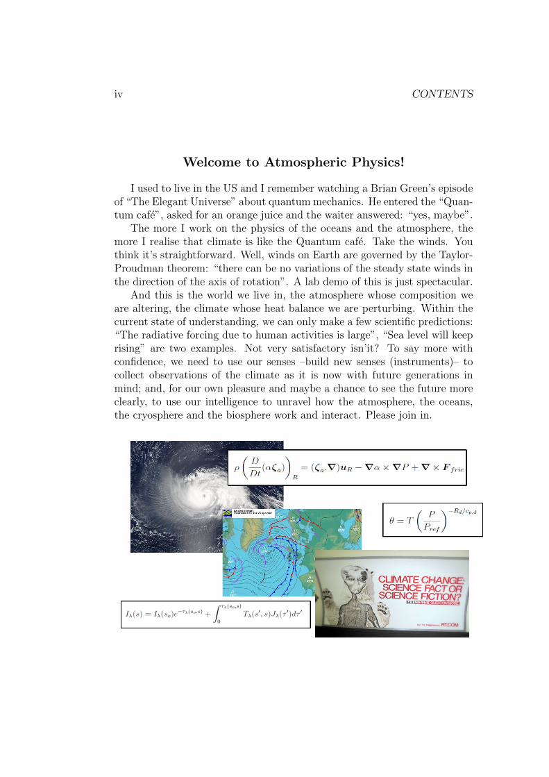
Welcome to Atmospheric Physics!
I used to live in the US and I remember watching a Brian Green’s episodeof “The Elegant Universe” about quantum mechanics. He entered the “Quan-tum cafe”, asked for an orange juice and the waiter answered: “yes, maybe”.
The more I work on the physics of the oceans and the atmosphere, themore I realise that climate is like the Quantum cafe. Take the winds. Youthink it’s straightforward. Well, winds on Earth are governed by the Taylor-Proudman theorem: “there can be no variations of the steady state winds inthe direction of the axis of rotation”. A lab demo of this is just spectacular.
And this is the world we live in, the atmosphere whose composition weare altering, the climate whose heat balance we are perturbing. Within thecurrent state of understanding, we can only make a few scientific predictions:“The radiative forcing due to human activities is large”, “Sea level will keeprising” are two examples. Not very satisfactory isn’it? To say more withconfidence, we need to use our senses –build new senses (instruments)– tocollect observations of the climate as it is now with future generations inmind; and, for our own pleasure and maybe a chance to see the future moreclearly, to use our intelligence to unravel how the atmosphere, the oceans,the cryosphere and the biosphere work and interact. Please join in.
CONTENTS v
Practical things
These notes contain only the basic information discussed in the lectures(the latter are where emphasis is on the physical interpretation and schemat-ics). My aim in writing them is to provide you with a support and a clearknowledge of what is examinable (=what is in the notes). The formal “Aimsand objectives” for the course follows next page. In terms of reading:
• I recommend the excellent textbook by Wallace and Hobbs (‘’Atmo-spheric Sciences: an introductory survey”) as a companion for thecourse (the library has many copies).
• You might also enjoy reading “Clouds in a glass of beer: simple ex-periments in atmospheric physics” by Craig Bohren (cheap paperbackDover edition), as well as the textbook by John Marshall and AlanPlumb entitled “Atmosphere, Ocean and Climate Dynamics: An in-troductory text” and the older but concise and clear “The Physics ofAtmospheres” by John Houghton. I have also included further refer-ences in some chapters.
Each chapter contains a set of problems, whose solutions will be providedas we go along. Some sections in the notes are highlighted with a ? whichindicates that they are a little more challenging.
There are a couple websites which I would like to emphasize:
• https://earth.nullschool.net This is a wonderful website depictingthe state of the atmosphere and the (surface) ocean in nearly real time.The data comes from a global operational forecast system from the US(which is constrained by many observations) and satellite observationsfor the ocean. The graphics are stunning and there is so much to learnand wonder spending time on it (believe me it beats Youtube).
• http://www.ecmwf.int/s/ERA-40 Atlas/docs/ An excellent sourceof quick plots for the mean atmospheric state. This climatology hasbeen developed at a big European centre for weather forecast and cli-mate in Reading (ECMWF).

vi CONTENTS
• http://www.sp.ph.ic.ac.uk/aczaja/EP ClimateModel.html This isa simple climate model which I will at times use during the lectures. Itis well documented and cheap to run (either in Matlab or in Python,thanks to the hard work of an undergraduate student Joe Marsh Ross-ney).
Please do not hesitate to come to Office Hours (Thursdays, 11.30-12.30;Fridays, 1-2pm) for further help or to give me feedback on the course. Youare also welcome to make any suggestions by email at [email protected].

CONTENTS vii
Aims and Objectives for the Course
Aims To provide students with an understanding of the physics behind thestructure, the dynamics and the energetics (radiative transfer, thermodynam-ics) of the Earth’s atmosphere (emphasis on troposphere and stratosphere).
Objectives By attending the course, the students should:
• be able to describe the basic structure of the Earth’s atmosphere andthe climate system
• be able to use fundamental thermodynamics to derive expressions forthe variation of temperature, pressure, and density with height
• understand the concept of potential temperature and how it relates tostability, buoyancy frequency and temperature lapse rate
• understand the concept of radiative-convective equilibrium
• know the components of the Earth radiation balance
• understand the concepts of optical depth, radiation intensity, irradi-ance, and transmission of radiation
• be familiar with Schwarzschild’s equation of radiative transfer and beable to solve it for both solar and thermal radiation streams undersimple conditions
• be able to derive a simple model of the greenhouse effect
• be able to compute radiative heating rates given irradiances
• know the forces acting on a parcel of air and apply Newton’s 2nd Lawto deduce the equations of motion for a compressible gas on a rotatingplanet
• know how to apply scale approximations to the equations of motion(e.g., hydrostatic and geostrophic approximations, Rossby number)
• understand why vorticity is a useful concept for the study of atmo-spheric motions
• understand the effect of water on the radiative, thermodynamic anddynamical aspects of Atmospheric Physics
• understand the concept of radiative anthropogenic forcing and the basicresponse of the atmosphere to this forcing

viii CONTENTS

Chapter 1
An overview of the atmosphere
key concepts: well mixed gases, “dry” and “moist” air, measures of watervapour in air, top-of-the-atmosphere (TOA), global budgets of mass, heatand angular momentum.
Before we dive into quantitative analysis of the atmosphere it is importantnot to loose sight of some of the big questions. Here are a few which Imentioned in the introduction lecture (ppt slides on Blackboard):
• The atmosphere is our common environment. It is the fluid we allbreath. We say that we are connected with the internet but we areactually physically connected because we constantly share and recycleair molecules through our lungs. When the surface winds come fromthe South, I am breathing air which was a day or two before breathedin and out by someone in Spain or maybe Africa. This is becausetypical north-south velocities in a weather system are on the order of10ms−1 so an air parcel covers approximatively 10 of latitude in oneday (≈ 105s).
• Randomness. The tropical Pacific ocean is one area of the globe withthe most observations (ocean and atmosphere) because it is the siteof a major reorganisation of the wind, temperature and precipitationpatterns known as El Nino. Every few years, heat builds up in thewestern Pacific ocean and is suddenly released eastward and poleward,shifting entirely the tropical precipitation pattern. The atmosphereis “rung” by this shift and generates waves propagating towards theNorthern and Southern Hemispheres, perturbing the weather systemsthere. El Nino is also the climate phenomenon with the best theo-ries. Or so we thought. In the summer of 2014, all El Nino experts
1

2 CHAPTER 1. AN OVERVIEW OF THE ATMOSPHERE
predicted that the largest event ever recorded will develop during thefollowing winter. It simply did not happen! No El Nino event at all(see McPhaden, 2015). Imagine telling your friends you’re an expert atsomething, predicting the largest anomaly ever seen...and things go onperfectly normally. This shows that there is a lot more to understand.Maybe, fundamentally, deterministic predictions of the coupled atmo-sphere - ocean system are impossible. Maybe this system is a bit like aquantum mechanics sytem, with only probablistic statements possible.
• Observations. In fifty or a hundred years, we will still need to check thatour numerical models of the climate are accurate. The ones we have anduse now have been only tested over a short period of time (true globalobservations of the atmosphere only started with the satellites launchedin the 1970s –in the ocean this type of coverage simply does not existbelow about a 1000m) and one should not be overconfident regardingtheir accuracy (see point above). People in fifty or a hundred years willnot be able to travel back in time and make these observations. It isour duty to do so. Even if like me, you are not someone developinginstruments, you can help those who do by finding the most usefulquantity to observe. And by using the data in your own way, you helpmaintain the observational network.
1.1 Atmospheric composition
The most abundant substance in the atmosphere is diatomic nitrogen (N2),which accounts for 78% of the air molecules we breath. Most of the nitrogenon Earth is actually stored in the atmosphere (3.9× 10¹⁸kg), with the Lito-sphere (Earth’s crust) coming second (≈ 2× 10¹⁸kg) The large atmosphericreservoir of nitrogen reflects the outgassing from the Earth’s interior in theearliest stage of its history and the great stability of the N2 molecule.
Next in abundance comes “free” oxygen (O2), which represents 21% ofatmospheric molecules. The Earth is unique in having so much of its atmo-sphere made up of diatomic oxygen, and there is little doubt that this reflectsthe presence of life early in its history (it is believed that oxygen started toaccumulate in the atmosphere about 2Gyr ago, when the production of O2
by bacteria exceeded the consumption of O2 by iron ions dissolved in theoceans).
The percentages given above assume that any given sample of air has thesame composition. In practice, this is only true for gases whose residencetime in the atmosphere is long compared to the time it takes for atmospheric
1.1. ATMOSPHERIC COMPOSITION 3
motions to mix (from a few days to a few months). This is for example thecase for N2, O2 as well as argon (Ar,≈ 0.9% of air molecules) and carbondioxide (CO2,≈ 0.04% of air molecules), the next two most abundant speciesafter N2 and O2. Water vapour has a highly variable distribution (withconcentrations which can be greater than that of Ar locally) depending ontime and location because it can be quickly removed from the atmospherethrough rainfall. The height at which mixing by motions is not vigorousenough to maintain a uniform composition is about 100km (the turbopause).
For the troposphere (the lowest layer of atmosphere where temperaturedecreases with height, roughly from the Earth’s surface to a height z =10km) and stratosphere (the layer above the troposphere where temperatureincreases with height, from about z = 10km to z = 50km), which will bethe focus of the course, it is convenient to simplify atmospheric compositionby considering “dry air”, a mixture of N2, O2, Ar, CO2 and other tracegases, and “moist air” (water vapour). The primary reason for this is phasechange: as we’ll see in Section 1.5, there is a net heat gain by the atmospherethrough the hydrological cycle (latent heat) whereas this does not occur forother species (N2, O2, etc, although they are also exchanged between theatmosphere and the Earth’s surface). It is thus important to keep trackof local concentrations of water vapour. A useful measure of the “distanceto equilibrium of phases” is given by relative humidity (RH), the ratio ofthe vapour pressure e of a sample to the vapour pressure in thermodynamicequilibrium of phases (eeq(T ), a sole function of temperature T from theThermodynamic year 2 course):
RH ≡ e
eeq(1.1)
NB: This is just a definition. In thermodynamic equilibrium RH = 1 butthis condition is rarely met in the atmosphere (for example, it is in the coreof deep clouds but not in the accompanying donwdrafts which are too dry fore to match eeq(T ) and thus are air masses with RH < 1).
At a given temperature T and volume V , the pressure of “dry air” Pdobeys the ideal gas law to an excellent approximation,
PdV = NdkBT (1.2)
as does water vapour,eV = NvkBT (1.3)
In these two equations, kB is Boltzmann’s constant while N denotes the num-ber of molecules (the subscripts d and v will be used throughout the coursefor dry air and water vapour, respectively). Note that the total pressure P

4 CHAPTER 1. AN OVERVIEW OF THE ATMOSPHERE
of a given sample of air is simply the sum of Pd (the partial pressure of dryair) and e (the partial pressure of water vapour), as result known as Dalton’slaw,
P = Pd + e (Dalton’s law) (1.4)
Atmospheric pressures are usually expressed in hPa where 1hPa = 100Pa(you might also find pressures expressed as millibar (1mb = 10−3bar), inwhich 1bar = 105Pa).
Because of the very large number of molecules in the atmosphere, it isconvenient to rewrite the ideal gas law as,
PdV
Ndµd=kBµdT (1.5)
in which µd is the mass of a “dry air molecule” (µd =∑Niµi/
∑Ni where µi
is the mass of molecule i of which there are Ni in the sample considered –thesum is carried over i = N2, O2, Ar, CO2, etc). Introducing the specific volumeof dry air αd, and the gas constant for dry air Rd = kB/µd = 287J kg−1 K−1,this becomes,
Pdαd = RdT (1.6)
Likewise, for water vapour,
eαv = RvT (1.7)
with Rv = kB/µH2O = 461J kg−1 K−1.
1.2 Mass
1.2.1 Pressure as a measure of mass
In layers of air of large horizontal extent, and in particular for the globalhorizontal average, there is an approximate balance between gravity and thevertical pressure gradient force,
ρg = −∂P∂z
(hydrostatic equation) (1.8)
Note the minus sign, which expresses that pressure must decrease with heightto be able to oppose the downward acceleration due to gravity.
One interesting use of this equation is to integrate it in the vertical as,
P (z) =
∫ +∞
z
ρgdz (1.9)
1.2. MASS 5
in which we have used the fact that pressure vanishes at sufficiently largeheights. The discussion in section 1 showed that this is a good approximationfor z 8km and this loosely defines the “top-of-the-atmosphere” (TOAthroughout the course). The corresponding layer of air is still very thincompared to the Earth radius so that one can approximate g in the integralby its surface value g = 9.81ms−2,
P (z)/g =
∫ +∞
z
ρdz (1.10)
This shows that atmospheric pressure can be thought of as a mass mea-surement since ρdz is simply the mass per unit area sandwiched betweenheights z and z + dz. A couple of straightforward applications of this equa-tion are worth mentioning. An order of magnitude for the surface pressureis Ps = 1000hPa while for the tropopause it is 100hPa. This shows that thetroposphere contains about ' (1000− 100)/1000 = 90 % of the mass of theatmosphere. Conversely, since the pressure P in (1.10) is the total pressure(P = Pd + e), and that e at the Earth’s surface is typically 10hPa in theglobal and annual mean, water vapour contributes to ' 10/1000 = 1 % ofatmospheric mass.
Technical sidenote: units of pressure. Pressure is usually expressed in hPa =100Pa in atmospheric sciences. You might also find the use of millibars (mb,1mb = 10−3bar where 1bar = 105Pa).
1.2.2 Measures of water in air
A given sample of air is described, besides its temperature and pressure, byits mass of dry air md (see previous section), water vapour mv, liquid waterml and ice water mi. It is common practice to introduce ratios of thesequantities:
qv ≡mv
md +mv +ml +mi
(specific humidity) (1.11)
ql ≡ml
md +mv +ml +mi
(specific liquid water content) (1.12)
qi ≡mv
md +mv +ml +mi
(specific ice water content) (1.13)
qd ≡md
md +mv +ml +mi
(specific mass of dry air) (1.14)
6 CHAPTER 1. AN OVERVIEW OF THE ATMOSPHERE
In terms of size, because there is so little amount of water in the air, qd qv,and typically qv (ql, qi). Note that qd = 1−(qv+ql+qi). The total specificamount of water is denoted by qt ≡ qv + ql + qi.
Sometimes, mass mixing ratio, rather than specific humidity is used. Thedifference is that, for example for water vapour (mixing ratio rv), mixing ratioinvolves taking the ratio of mv to md rather than mv to mv +md +ml +mi,i.e.,
rv ≡mv
md
(mass mixing ratio) (1.15)
The air density ρ is defined according to,
ρ =md +mv +ml +mi
V(1.16)
in which V is the total volume occupied by the sample (the sum of thevolumes occupied by the gas, liquid and solid phases). As a result, thedensity of dry air ρd = md/V = (m/V )(md/m) = ρqd, and, likewise, thedensity of water is ρt = (mv +ml +mi)/V = (m/V )(mv +ml +mi)/m = ρqt.
The total amount of water vapour in an atmospheric column, or totalprecipitable water (TPW), is
TPW =
∫ ∞0
ρqvdz (1.17)
To get a feel for the surprising result to come below, let’s use the simplemodel ρ = ρse
−z/Hs and qv = qse−z/Hq in which Hs is the scale height, Hq
a scale height for moisture (Fig. 1.1) and ρs, qs refer to surface density andspecific humidity, respectively. One can then estimate that,
TPW ≈ ρsqsH with H =HsHq
Hs +Hq
(1.18)
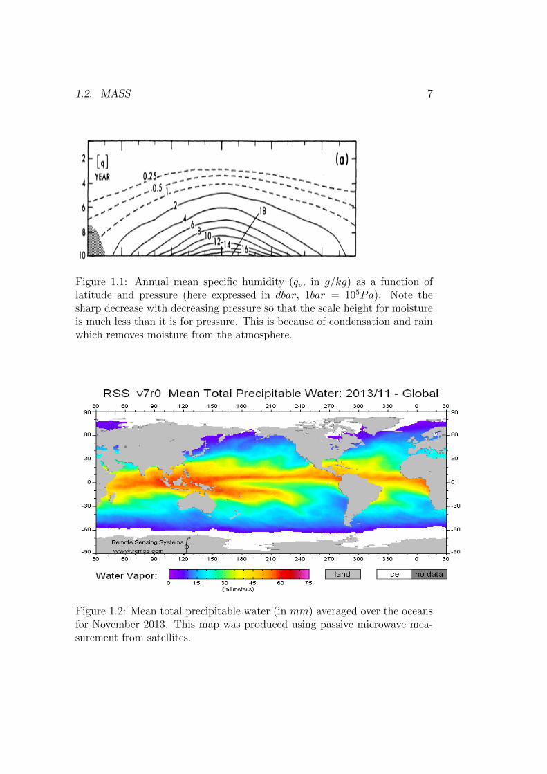
Expressed in mm of water per unit area by dividing this quantity by thedensity of water, we find typically that the atmosphere holds somethinglike 20mm of precipitable water in vapour form (for ρs = 1.2kgm−3, qs =10g/kg,Hs = 7km,Hq = 3km). Observed values (Fig. 1.2) are indeedwithin that range. This is somewhat surprising since it can rain much morethan that in a matter of a few hours but it can be rationalized by thinkingof storms (the cyclones at our latitudes and even more so hurricanes) as veryefficient machines collecting water vapour over very large distances, condens-ing it, and “dumping” it as rain: this is the “dehumidifier view” of cyclones.
1.2. MASS 7
Figure 1.1: Annual mean specific humidity (qv, in g/kg) as a function oflatitude and pressure (here expressed in dbar, 1bar = 105Pa). Note thesharp decrease with decreasing pressure so that the scale height for moistureis much less than it is for pressure. This is because of condensation and rainwhich removes moisture from the atmosphere.
Figure 1.2: Mean total precipitable water (in mm) averaged over the oceansfor November 2013. This map was produced using passive microwave mea-surement from satellites.

8 CHAPTER 1. AN OVERVIEW OF THE ATMOSPHERE
1.3 Main features of the atmosphere
Based on the ppt slides for this chapter (to which you are referred to forillustrations), the main features of the atmosphere are:
• a well mixed structure up to ≈ 100km in terms of constituents, with anear exponential decay of pressure and number densities with height.The associated scale is on the order of 8km for the well mixed layer1.
• a rich temperature structure, with, in some regions, temperature de-creasing with height and poleward, but in some regions temperatureincreasing upward and poleward (Fig. 1.3, top panel). The simplestview (global average as a function of height) is schematized in Fig. 1.4,introducing the troposphere, the stratosphere and the mesosphere. Thecourse will focus on the first two of these where 99.9 % of the mass ofthe atmosphere resides.
• the presence of strong zonal (=along a latitude circle) time mean jetswith windspeeds in excess of 30m/s. These are mostly found goingfrom west to east (e.g., the tropospheric Jet Stream) but also existsseasonally from east to west (mesospheric jets) –see Fig. 1.3, bottompanel. At the Earth’s surface, westerlies are found poleward of 30 oflatitude, and easterlies (“Trade winds”) are found equatorward of thatlatitude. The atmosphere is in a state of “superrotation”, an air parcelin the tropospheric Jet Stream coming back to its initial position inabout 23h, not 24h! We’ll prove in Chapter 4 that these jets are in“thermal wind balance”, meaning that their variations with height areconstrained by the horizontal temperature gradients.
• the presence of smaller time mean velocities in the North-South direc-tion (a few ms−1). These are predominantly seen in the Hadley cellat low latitudes, with rising motions near the equator and descendingmotion along ≈ 30. Such “meridional cells” (in the latitude-heightplane) also exist in the stratosphere and mesosphere but the associatedmass transport is much weaker than that of the Hadley cell.
• its convective nature (Fig. 1.5) on scales ranging from a few km tothousands of km (planetary scale). Updraft motions are associated
1From Boltzmann’s principle we would expect the ratio of distribution of a moleculeof mass m at height z1 and z2 to obey n1/n2 = emg(z1−z2)/kBT where g is gravity and Ttemperature. This provides a different scale height for each molecule according their mass(kBT/mg), which is not observed below 100km (the “turbopause”). It is observed above100km.

1.4. WHATDRIVES ATMOSPHERICWINDS,WEATHER PATTERNS, ETC?9
with phase change and the formation of rain, snow and other hydrom-eteors. The convection involves mostly upward/downward motions inthe Tropics, but sloping (i.e., upward and poleward, downward andequatorward) motions at higher latitudes as we’ll discuss in Chapter 3.
• The fundamental role of water vapour. Not only does it affect atmo-spheric motions through its effect on buoyancy (condensational heat-ing, evaporative cooling add or remove buoyancy to air parcels, as we’llsee in Chapter 3), but water vapour is also the main greenhouse gas(as we’ll see in Chapter 2). Because the oceans occupy 70% of theEarth’s surface and because surface evaporation depends on surfacetemperature, water vapour couples the state of the oceans to that ofthe atmosphere.
• The atmosphere is only one component among many (oceans, cryosphere,biosphere, the deep Earth, etc) setting the Earth’s climate.
• The atmosphere has a mind of its own. The “butterfly effect” wasintroduced by MIT’s meteorologist Ed Lorenz to illustrate the sensitiv-ity of the atmospheric state to initial conditions. Predictability beyonda week or so arises from slower changes in boundary conditions (seasurface temperature, sea ice, vegetation cover, etc). In addition, theatmosphere is turbulent, with energy transfers towards small scale butalso, more surprisingly, towards large scales. This makes the standarddefinition of weather (=state of the atmosphere at a given time) andclimate (=statistics over a long enough time period) a bit ambiguous.One should really add a “grey zone”, the low frequency variability ofthe atmosphere, i.e., fluctuations which can persist for longer than aweek (e.g., blocking conditions associated with long lived cold spells inthe UK like occurred in 2009-2010). These are not “weather”, nor arethey “climate”.
1.4 What drives atmospheric winds, weather
patterns, etc?
A few simple ideas are worth mentioning:
• There is an asymmetry between the radiation received from the Sun andthat emitted by the Earth (surface + atmosphere). Photons emittedby the Sun have wavelengths smaller than a few microns while photons

10 CHAPTER 1. AN OVERVIEW OF THE ATMOSPHERE
Figure 1.3: Seasonal and zonal (i.e., averaged along a latitude circle) meanatmospheric temperature (top panel, in degree Celcius) and zonal wind (bot-tom panel, in ms−1 with a contour interval of 10ms−1, W indicating westto east winds and E east to west winds) as a function of height/pressure(vertical axis) and latitude (horizontal axis). Figure taken from Wallace andHobbs’ textbook.

1.4. WHATDRIVES ATMOSPHERICWINDS,WEATHER PATTERNS, ETC?11
Figure 1.4: Global, annual mean atmospheric temperature as a function ofheight/pressure.

12 CHAPTER 1. AN OVERVIEW OF THE ATMOSPHERE
Figure 1.5: Global composite infrared map on 9 March 2004. White is coldon this map and, in most regions, indicates the presence of upper level clouds.Notice the “spotty” nature of the convection in the Tropics and the “wavi-ness” in middle and high latitudes. You can find many of those maps (aswell as animations) on the MetOffice website.
emitted by the Earth have wavelength larger than a few microns (Fig.1.6). As a consequence, an atmospheric layer exchanges radiation withother atmospheric layers and the Earth’s surface (and these exchangestend to cancel out), but there is no two-way exchange with Space andthe atmosphere cools radiatively in the infrared (Fig. 1.7)
• In addition, solar photons are in comparison much less absorbed by theatmosphere than terrestrial photons. This means that, to zero order,the atmosphere can be thought of as transparent to solar radiation,the latter being primarily absorbed by the Earth surface. So the at-mosphere is heated from below by the Earth’s surface, and it coolsradiatively to Space (previous point). This is a very unstable situa-tion, a bit like a pan of water boiling on a cooker: the atmosphere isin a state of global convection.
• The radiative cooling to space is relatively uniform spatially but incom-ing solar radiation peaks at low latitudes as a result of the sphericalshape of the Earth and the large Earth-Sun distance. This means thatin addition to the heating from below and cooling aloft, there is alsoa net cooling at high latitudes and net heating at low latitudes (Fig.

1.4. WHATDRIVES ATMOSPHERICWINDS,WEATHER PATTERNS, ETC?13
Figure 1.6: Planck function Bλ (see Chapter 2) for a body at T = 5780K(red) and T = 255K (blue) in a log-log scale. The red dashed curve rescalesthe red one by a factor π(Rsun/1AU)2/2π where Rsun is the Sun’s radius, toaccount for the different solid angles associated with solar (π(Rsun/1AU)2)and terrestrial (2π) radiation.

14 CHAPTER 1. AN OVERVIEW OF THE ATMOSPHERE
Figure 1.7: A schematic of the radiative exchanges for an atmospheric layer.(Left) All exchanges are represented: the layer absorbs radiation from aboveand below (including the Earth’s surface), and it emits to other layers aboveand below (small arrows). In addition it also emits radiation to Space (largearrow) but does not absorb solar radiation. (Right) Assuming the inter-layersand surface exchanges nearly cancel, which is not a bad approximation iftemperature variations are sufficiently weak and the atmosphere is sufficientlyopaque, this leaves a net loss of energy to Space. Picture taken from Wallaceand Hobbs’ textbook.

1.4. WHATDRIVES ATMOSPHERICWINDS,WEATHER PATTERNS, ETC?15
1.8). Laboratory experiments with rotating tanks cooled at the out-side and heated at the inside, to mimic the equator-to-pole contrast inheating, indicate that the resulting motion can be irregular with clearqualitative similarities with the atmosphere.
The above arguments are rough but they give a feel for the key role ofradiation as a driver of atmospheric motions and weather systems (a fullestimate of the various energy fluxes is given in Fig. 1.9). The laboratoryexperiments mentioned in the last bullet point also indicate the very strongconstraint imposed by the rotation of the Earth (rotation rate Ω). It is onlywhen the latter is fast enough that the simulated flows bear a qualitativeresemblance to the atmosphere. This is because the flow not only transportsheat from the equator to the pole, to balance the deficit highlighted in Fig.1.8, but also transports atmospheric angular momentum (L). The latter issimply the azimuthal velocity (u + ΩR cosφ), R being the Earth radius, φlatitude and u the west-to-east velocity relative to the rotating Earth, timesthe distance to the axis of rotation (R cosφ):
L = R cosφ(u+ ΩR cosφ) (1.19)
Atmospheric angular momentum has thus a contribution from the Earth’ssolid body rotation, or planetary contribution (ΩR2 cos2 φ), and a contri-bution from relative motions (uR cosφ). In practice, the former dominatesover the latter. For example at the latitude of the subtropical Jet Stream(≈ 30), one has u ≈ 30ms−1 while ΩR cos(30) ≈ 400ms−1. Note that inthis derivation, L is angular momentum per unit mass, and that I have usedthroughout R + z ≈ R where z is the height of an atmospheric ring abovethe Earth’s surface.
Integrated over the whole mass of the atmosphere L is approximativelyconstant, i.e.,
∂
∂t
∫∫∫ρLdV ≈ 0 (1.20)
This implies an intriguing compensation between the Tropics, in which thesurface winds are westward (Trade winds) and thus where the atmosphereis gaining angular momentum (friction accelerates low levels in the senseof the Earth’s rotation), and higher latitudes, where the surface winds areeastward and thus where the atmosphere is loosing angular momentum. Aswe shall see in Chapter 4, the Tropics and extra-tropics are coupled throughthe propagation of a certain type of waves called Rossby waves. The latterare excited mostly from midlatitudes by the storm we experience daily andas they propagate equatorward they transport angular momentum poleward.
16 CHAPTER 1. AN OVERVIEW OF THE ATMOSPHERE
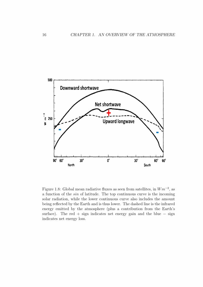
Figure 1.8: Global mean radiative fluxes as seen from satellites, in Wm−2, asa function of the sin of latitude. The top continuous curve is the incomingsolar radiation, while the lower continuous curve also includes the amountbeing reflected by the Earth and is thus lower. The dashed line is the infraredenergy emitted by the atmosphere (plus a contribution from the Earth’ssurface). The red + sign indicates net energy gain and the blue − signindicates net energy loss.

1.4. WHATDRIVES ATMOSPHERICWINDS,WEATHER PATTERNS, ETC?17
Figure 1.9: Recent observations of the Earth’s energy budget. All quotednumbers represent Wm−2. Solar fluxes are in beige and infrared fluxes inpink. From Stephens et al. (2012).

18 CHAPTER 1. AN OVERVIEW OF THE ATMOSPHERE
Thus, the storms we experience daily across the UK provide the mechanicalcoupling between vastly distant parts of the Earth.
Finally, note that this compensation between surface easterlies and west-erlies can only be approximate since torques are also exerted as a result of thepressure contrast across the major mountains of the Earth like the Himalayasand the Rockies.
1.5 Further reading
-Stephens et al., 2012: An update on Earth’s energy balance in light of thelatest global observations, Nature Geosciences, 5, 691-696.-Lovelock, 1979: Gaia, a new look at life on Earth, Oxford University Press.This book (and the many sequels) offers a fascinating discussion of atmo-spheric composition and demonstrates the broadness of the subject.-McPhaden, M., 2015: Playing hide and seek with El Nino, Nature ClimateChange, 5, 791-795.
1.6 Problems
Q1 In the (zonal mean) stratosphere and mesosphere, where (latitude, alti-tude, season) are found: (i) the coldest temperature (ii) the warmest tem-perature (iii) the strongest westerly wind? You might find useful to refer tothe slides for Lecture 1.
Q2 Why are deserts more likely to be present in the sub-tropics than ineither the tropics or mid-latitudes?
Q3 These two subquestions are independent of each other.
(i) At 25 km altitude, where atmospheric pressure is Po ≈ 25hPa andtemperature is To ≈ 220K, the mass mixing ratio of ozone is 10 partsper million. Compute (a) density and (b) partial pressure of ozonestating any assumptions made. Data: Rd = 287JK−1kg−1.
(ii) Express the fraction of water vapour molecules in ppm (part per mil-lion) in a sample of air where the partial pressure of water vapour ise = 10hPa and that of dry air Pd = 1000hPa. Compare the number ob-tained with the current fraction of carbon dioxide molecules (400ppm).
Q4

1.6. PROBLEMS 19
Table 1.1: Data for Q5. The number in parentheses refer to the molecularmass of the main atmospheric constituents.
Planet Major atmospheric Mean lower Mass Radiuscomponent temperature (K) kg km
Venus CO2 (44) 750 4.87× 1024 6,051Earth N2, O2 (29) 280 5.97× 1024 6,371Mars CO2 (44) 250 6.42× 10²³ 3,397
Jupiter H2 (2) 123 1.90× 1027 71,490
(i) One kg of air of specific humidity q1 = 10g/kg is mixed with one kg ofair of specific humidity q2 = 5g/kg. What is the specific humidity q3of the air mass after mixing? You may assume the conditions are suchthat no phase change occurs.
(ii) In the jargon of Thermodynamics, is specific humidity an intensive oran extensive variable?
Q5 (i) Show that in an isothermal atmosphere (T = To) the pressure decaysexponentially with height with a scale Hs = kBTo/mg (the scale height), inwhich g is the gravity of the planet and m is the mass of an atmosphericmolecule. (ii) Estimate Hs in the lower atmosphere for each of the planetlisted in Table 1.1.
Q6 Show that the specific volume α of a sample of air can be approximatedas,
α ≈ αd(1− qt) (1.21)
in which αd = RdT/Pd is the specific volume of dry air (Rd being the gasconstant for dry air, Pd the partial pressure of dry air and T temperature).You might want to start by writing that α = (V +Vl+Vi)/(md+mv+ml+mi)in which V is the volume of the sample occupied by the gas phase, Vl and Vithat of the liquid and ice phases, respectively.
Q7 By inspection of a surface pressure map (for example from the on-lineERA40Atlas2), work out whether the Rocky mountains tend to increase ordecrease atmospheric angular momentum.
Q8 A simple view of the Tropics is that it is primarily independent of lon-gitude, i.e., rings of air flow upward at the equator in the ascending branch
2See the web link on Blackboard.

20 CHAPTER 1. AN OVERVIEW OF THE ATMOSPHERE
of the Hadley cell, and flow poleward at upper levels, conserving their angu-lar momentum. Estimate the implied zonal velocity u (relative to the solidbody rotation of the Earth) at 30 of latitude. How does it compare withthe observed velocity? Hint: you may assume that the relative velocity u ofthe ring is very small near the ground.
Q9 Using the numbers in Fig. 1.9, discuss whether the atmosphere can bereasonably described as transparent to solar radiation.

Chapter 2
Radiative heating and coolingof the atmosphere
Key concepts: solid angle, irradiance, radiation balance, greenhouse effect,Beer’s law, Schwarzschild’s equation, infrared cooling to Space.
2.1 Concepts and definitions
2.1.1 Intensity of radiation
The intensity of electromagnetic radiation at wavelength λ measures the en-ergy crossing a unit area perpendicular to the direction of propagation perunit time, per unit wavelength interval, and per unit solid angle (Fig. 2.1).The “per unit area” and “per unit time” are familiar, but the “per unit wave-length interval” and “per unit solid angle” is less so. The “per unit wave-length interval”, or “per wavelength” for short, is needed to account for thespectrum of electromagnetic radiation, the total energy flux being computedas the integral over all wavelengths (i.e.,
∫Fλdλ). In absence of scattering
or absorption, the intensity of radiation, denoted by Iλ, is conserved (see theAppendix if you’re interested to read more about this).
The “per unit solid angle” is included to represent the 3D nature ofelectromagnetic radiation. The radiation reaching P in Fig. 2.1 in a givendirection is made of an infinitesimal cone of rays, or “radiation pencil”, fillinga certain fraction of the sky. This fraction is measured by solid angle Ω,exactly like an angle is a measure of length on a unit radius circle (Fig. 2.2).Solid angle is expressed in steradians (sr) and the maximum solid angleattainable (the amount of space filled by the sky if we were floating in theair) is 4π ≈ 12.5sr (an hemisphere is 2π).
21
22CHAPTER 2. RADIATIVE HEATING AND COOLINGOF THE ATMOSPHERE
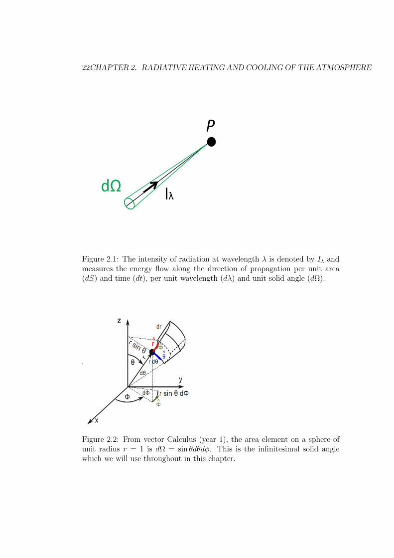
Figure 2.1: The intensity of radiation at wavelength λ is denoted by Iλ andmeasures the energy flow along the direction of propagation per unit area(dS) and time (dt), per unit wavelength (dλ) and unit solid angle (dΩ).
Figure 2.2: From vector Calculus (year 1), the area element on a sphere ofunit radius r = 1 is dΩ = sin θdθdφ. This is the infinitesimal solid anglewhich we will use throughout in this chapter.

2.1. CONCEPTS AND DEFINITIONS 23
Figure 2.3: Example of calculation of solid angle. The total solid angle ofthe Sun at a distance r is the sum over the angle θ (from 0 to α) of all thesmall solid angles 2π sin θdθ indicated by the black shell.
Example: Compute the solid angle of the Sun (radius R), as seen from adistance r to its center (Fig. 2.3). The Sun is seen by an observer on the
sphere of radius r with a solid angle Ω(r) =∫ 2π
0
∫ α0
sin θdθdφ = 2π(1− cosα)where the angle α satisfies tanα = R/r (note the right angle magenta triangledefining α in Fig. 2.3). It covers a solid angle Ω ≈ 2π very close to the source(α = π/2) and Ω ≈ π(R/r)2 for r R since 1 − cosα ≈ α2/2 when α issmall.
2.1.2 Blackbody radiation
As taught in Year 2 (Thermodynamics and Statistical Physics), blackbodyradiation is the radiation emitted by a body in thermal equilibrium. It isisotropic and only depends on the temperature T characterizing the equilib-rium, not on the nature of the material making the body. Its intensity, at a
24CHAPTER 2. RADIATIVE HEATING AND COOLINGOF THE ATMOSPHERE
given wavelength λ is given by the Plank function,
Bλ(T ) =2hc2λ−5
ehc/λkBT − 1(2.1)
which has units of Wm−2 per wavelength per solid angle.
2.1.3 Shortwave and longwave radiation
We saw in section 1.4 that there is a small overlap of the Planck functionsassociated with terrestrial (infrared) and solar (visible) emissions (Fig. 1.6–note the scaling of the Planck function by the solid angle of the Sun asseen from the Earth which is, from the calculation in section 2.1.1, equalto π(R/r)2). It is, as a result, common practice to separate “longwave” and“shortwave” radiations. Typically, 4µm is used as the separation between thetwo. As we shall see the difference in wavelength will lead to important differ-ences with respect to the role played by scattering and absorption/emissionin the conservation of radiation intensity for longwave (scattering negligible,absorption/emission important) and shortwave radiation (scattering impor-tant, absorption important, emission negligible).
2.1.4 Irradiance
The energy of radiation passing through an horizontal plane, per unit area ofthat plane, per unit wavelength is called the monochromatic irradiance Fλ.It requires integrating Iλ over solid angle (2π at most for either upward ordownward hemispheres) and taking into account the angle between the beamand the normal to the horizontal plane.
Consider for example the geometry in Fig. 2.4 and take the horizontalplane to be the x, y plane. The net downward radiation across the horizontalplane is made of several “radiation pencils”, each coming from different anglesθ with the z direction and the polar angle φ in the horizontal plane. It isthus a matter of summing over all these pencils, each of infinitesimal solidangle dΩ, and projecting onto the vertical Iλ → Iλ cos θ. Thus,
Fλ =
∫Iλ cos θdΩ (2.2)
or using dΩ = sin θdθdφ,
Fλ =
∫ 2π
φ=0
∫ π/2
θ=0
Iλ cos θ sin θdθdφ (2.3)
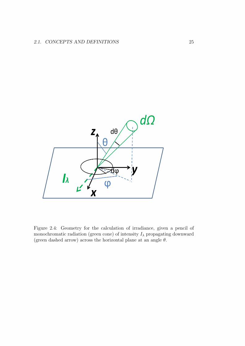
2.1. CONCEPTS AND DEFINITIONS 25
Figure 2.4: Geometry for the calculation of irradiance, given a pencil ofmonochromatic radiation (green cone) of intensity Iλ propagating downward(green dashed arrow) across the horizontal plane at an angle θ.

26CHAPTER 2. RADIATIVE HEATING AND COOLINGOF THE ATMOSPHERE
If the radiation is isotropic (i.e., independent of θ and φ), then the integralsimplifies to
Fλ = 2πIλ
∫ π/2
θ=0
cos θ sin θdθ = πIλ (2.4)
This result is exact for Blackbody radiation, for which Iλ = Bλ in (2.1), andso Fλ = πBλ (if one were to integrate the latter over all wavelengths, onewould obtain
∫πBλdλ = σT 4 in which σ is Stefan-Boltzmann’s constant).
NB: The irradiance just defined is, strictly speaking, a downward irradiance(we counted solid angles from above). We’ll denote it by F ↓λ in the following.We could also have computed the energy flux received from below, producing,for Iλ = Bλ, the same result: F ↑λ = πBλ (“upward irradiance”).
2.1.5 Kirchoff’s law
In practice, most components of the climate system do not behave like blackbodies, or only do so over a limited range of wavenumbers. For examplethe spectrum of most gases is made of sharp spectral lines, not a contin-uum; in addition, gases not only absorb radiation but also transmit it, unlikeblackbodies. We’ll see indeed in section 2.3 that the atmosphere is almosttransparent to infrared radiation in the 10−12µm, the so-called “atmosphericwindow” region (this is the spectral region chosen to make infrared picturesof the Earth since in this region infrared radiation either originates from theEarth’s surface or from cloud tops –see for example Fig. 1.5).
Surprisingly, even though the atmosphere does not emit according toBλ(T ), one can relate atmospheric emission and absorption to Bλ(T ) byusing Kirchoff’s law. To see this, define the emissivity of a particular bodyat temperature T (e.g., sample of air) according to,
ελ ≡ Iλ(emitted)/Bλ(T ) (2.5)
and define its absorbtivity as,
αλ ≡ Iλ(absorbed)/Iλ(incident) (2.6)
Kirchoff’s law states that, remarkably, irrespective of what the body is made,and irrespective of the nature of the radiation (isotropic or not),
ελ = αλ (Kirchoff’s law) (2.7)
NB: For a blackbody, ελ = αλ = 1 for all wavelengths. Note also thatKirchoff’s law only applies to systems in thermodynamic equilibrium with

2.1. CONCEPTS AND DEFINITIONS 27
their immediate surroundings (“local” thermodynamic equilibrium). Thiscondition is satisfied in the troposphere and the stratosphere but less soabove these regions.
2.1.6 The “solar constant”
We now apply the concept of radiation intensity and radiation pencils toestimate the amount of solar energy received per unit time by the Earth.This quantity is referred to as the solar constant So (in units of W ), althoughit fluctuates on many timescales (e.g., the decadal solar cycle)1
So we consider a point P on Earth at latitude φ and longitude γ (Fig.2.5) and first estimate the flux of energy received at that point. We will thensum over all points to obtain an expression for So. Because the Sun is so faraway from the Earth, we are going to treat the solar radiation received atP, at a given wavelength λ, as made of only one pencil of radiation. Indeed,as the calculation in section 2.1.1 showed, the Sun covers a solid angle angleδΩ ≈ π(Rs/1AU)2 where Rs is the Sun’s radius and 1AU (astronomical unit)is the mean Earth-Sun distance, that is a very small solid angle. This is justa mathematical way to say that the Sun covers only a small fraction of thesky. In addition, because the Sun is so far away form the Earth, we alsoapproximate the angle made between this pencil and the local vertical as thelatitude φ in a plane of constant longitude (Fig. 2.5). This is just saying thatwe are treating the impinging solar radiation as a plane wave. The Note thatFig. 2.5 only shows this projection in a plane of constant longitude. Youwould need to view the figure from the North pole to see the same effect in aplane of constant latitude, the result being that the angle between the penciland the local vertical in that plane is approximatively π/2− γ if 0 ≤ γ ≤ π).
With these approximations, the flux of energy per wavelength Φλ receivedfrom the Sun at P is,
Φλ ≈ Iλ cosφ sin γδΩ, (2.8)
so that the power Pλ per unit wavelength integrated over the Earth is simply,
Pλ ≈∫
ΦλR2 cosφdφdγ (2.9)
Note that in this expression the latitude φ is integrated from South to Northpole (−π/2 and π/2, respectively) but the longitude is only integrated over
1Once you realise how amazingly active the Sun is this is not a surprise. Have a look atthe fantastic movies NASA has made from the SDO mission (e.g., google “thermonuclearart SDO”).

28CHAPTER 2. RADIATIVE HEATING AND COOLINGOF THE ATMOSPHERE
Figure 2.5: Schematic for the calculation of the Solar constant. Note thatthe diagram is (obviously!) not on the correct scale.
the day hemisphere, i.e. from 0 to π. Inserting (2.8), we obtain,
Pλ ≈ IλδΩ
∫R2 cos2 φ sin γdφdγ = (IλδΩ)πR2 (2.10)
The above relation shows that, under our approximation of parallel im-pinging solar radiation, it all looks as if the Earth was a disk of radius πR2.Integrating over wavelength, we define the Solar constant as,
So ≡∫IλδΩdλ ≈ 1, 361Wm−2 (2.11)
so that the net power received by the Earth is SoπR2.
NB: This is a calculation valid for equinoctial conditions, or annual meanconditions, only. One would need to include the tilt of 23.5 of the eclipticplane to estimate the total energy gained at the solstices.
2.1.7 Radiation balance and emission temperature
A simplified energy balance for the Earth is given in Fig. 2.6. A fractionαP (the planetary albedo) of the Solar radiation discussed in the previoussubsection is reflected. At equilibrium, the same amount of power must be

2.1. CONCEPTS AND DEFINITIONS 29
Figure 2.6: Radiation balance of the Earth. The incoming solar radiationis treated as a parallel beam impinging on a spherical Earth. The outgoinginfrared radiation is isotropic.
lost by the Earth. The emission temperature is defined as the temperaturerequired to achieve this, were the Earth a perfect blackbody in the infrared:
πR2So(1− αP ) = 4πR2σT 4e (2.12)
leading to
Te ≡(So(1− αP )
4σ
)1/4
(2.13)
NB: note the factor of 4 coming from the geometry of the problem (planeradiation impinging a sphere as opposed to radial emission).
The idea of radiative balance at the TOA is an idealization. Globalconservation of energy requires that any imbalance be reflected in a changein heat content. This, in practice, is dominated by oceanic heat storage(largest heat capacity in the climate system) which fluctuates on very longtimescales (decades and longer) because of the slow ocean dynamics. Thusthe TOA net radiative fluxes are not expected to vanish on timescales shorterthan at least a few decades. We will come back to this in Chapter 5 whendiscussing anthropogenic climate change.
For Earth annual average, αP = 0.3 so that Te = 255K or −18C (verycold!). The Earth’s surface temperature is about 288K, or about +15C.
30CHAPTER 2. RADIATIVE HEATING AND COOLINGOF THE ATMOSPHERE
Thus, by contrast with the present model which omits entirely the atmo-sphere, we can say that the atmosphere is responsible for a≈ 288−255 = 33Kincrease in surface temperature. The way this works is disentangled in thesimple model coming next. Before doing so, it is worth mentioning a coupleof other interesting aspects of this model:
• it suggests that the bulk of the infrared radiation seen from Space orig-inates from the atmosphere itself rather than from the surface because255K is found typically at an altitude of 5km above the Earth’s surface.
• the Planck function for a blackbody at 255K is centered near 15µm(Fig. 1.6). This happens to be a wavelength at which the CO2 moleculeabsorbs strongly radiation, hence the strong “leverage” of CO2 on cli-mate.
2.2 A simple model of the greenhouse effect
We consider a 0D model of radiative balance (averaged over the whole Earth’ssurface area and expressed in Wm−2) and go a little beyond the previoussection by explicitly introducing the surface temperature Ts (Fig. 2.7).
In the shortwave, the solar flux impinging at the TOA is still So(1−αP )/4which we denote by Fo. We further assume that only a fraction Tsw ofthis radiation reaches the surface, to account for absorption by atmosphericmolecules and aerosols. (we’ll call Tsw the transmissivity of the atmospherein the shortwave in the following). From Kirchoff’s law, if some radiationis absorbed it must also be emitted. However, at terrestrial temperaturethe emission in the range of wavelengths where the bulk of solar radiationresides is negligible, and ελBλ(T ) αλIincoming. As a result, even thoughαλ = ελ for wavelengths λ in the shortwave part of the spectrum, we cansafely neglect the emission of shortwave radiation by the atmosphere.
In the longwave, we take the atmosphere to be at constant temperatureTa and denote by Fa the longwave flux it emits upward and downward. Thesurface is treated as a blackbody, thus emitting Fs = σT 4
s upward. A frac-tion TLW of this radiation reaches the top-of-the-atmosphere (we’ll call thisfraction the transmissivity of the atmosphere in the longwave). Fig. 2.7summarizes the energy flows.
We can predict what the surface temperature should be solely from energyconservation arguments. At equilibrium, the net flow of energy across anysurface must be zero. Applying this at the Earth’s surface yields (see Fig.2.7):
FoTsw + Fa = Fs (2.14)

2.2. A SIMPLE MODEL OF THE GREENHOUSE EFFECT 31
Figure 2.7: A simple model of the greenhouse effect. TOA denotes the“top-of-the-atmosphere” where pressure vanishes. The shortwave fluxes areindicated in black, the longwave ones in blue.

32CHAPTER 2. RADIATIVE HEATING AND COOLINGOF THE ATMOSPHERE
while, at the “top-of-the-atmosphere”, it produces:
Fo = Fa + FsTlw (2.15)
By assumption Fs = σT 4s while, using (2.13), Fo = σT 4
e . As a result,after elimination of Fa from the above two energy conservation equations, weobtain,
Ts = Te(1 + Tsw1 + Tlw
)1/4 (2.16)
This equation is remarkably simple and shows that the surface temper-ature and the emission temperature differ only by a factor proportional tothe transmissivities in the shortwave and the infrared. If there were no at-mosphere, Tsw = Tlw = 1 and Ts = Te = 255K. With an atmosphere, andif Tsw > Tlw, the surface temperature will then exceed Te. In the Earthatmosphere, Tlw ≈ 0.2 while Tsw ≈ 0.9, leading to Ts ' 286K.
The agreement of this prediction with the observed Ts = 288K is fortu-itous because of the extreme simplicity of the model (isothermal atmosphere,surface treated as a blackbody). The key point though is that because the at-mosphere is more transparent to shortwave than it is to longwave (Tsw > Tlw),there is a “recycling” of energy towards the surface:
FoTsw + Fa = Fo1 + Tsw1 + Tlw
> Fo (surface heating) (2.17)
The added heating leads to a larger surface temperature –this effect is calledthe greenhouse effect.
2.3 Beer’s law
NB: The “atmospheric window”, absorption, emission and scattering of ra-diation by atmospheric molecules and aerosols is dicussed in the ppt slide forthis chapter.
Consider a monochromatic beam of wavelength λ and of intensity Iλ. Wewant to derive the change in intensity (dIλ) of this beam along its directionof propagation (measured by the coordinate s). This change is caused ei-ther because some air molecules scatter the radiation (net loss of radiationintensity along the path but no change in radiation intensity integrated overall directions), or absorb it (net loss of radiation intensity along the pathbut no change in radiation intensity in other directions). If we denote by qathe mass of these molecules per unit mass of air, ρqa is the mass of these
2.4. SCHWARZCHILD’S EQUATION 33
molecules per unit volume and ρqads is the mass of those molecules per unitarea perpendicular to the direction of propagation.
Beer’s law states that,
dIλ = −Iλkλρqads (2.18)
in which kλ (in m2kg−1), called the extinction coefficient, measures the in-tensity of absorption or scattering of radiation of wavelength λ,
kλ = βλ(absorption) + σλ(scattering) (2.19)
Equation (2.18) can be integrated along the path of the beam as,
Iλ(s) = Iλ(so)e−
∫ ssokλρ(s
′)qa(s′)ds′ (2.20)
In this expression so is a starting point where the radiation intensity is Iλ(so).It is convenient to introduce the following quantities,
Tλ(so, s) = e−∫ ssokλρ(s
′)qa(s′)ds′ (transmittance) (2.21)
τλ(so, s) =
∫ s
so
kλρ(s′)qa(s′)ds′ (optical depth) (2.22)
Note that both τλ > 0 and 0 ≤ Tλ ≤ 1 are non dimensional functions (i.e.,they are just numbers, without SI units). One measures the opacity of theatmospheric layer over a given path (τλ, the larger the more opaque the layer;hardly any radiation escapes a layer with optical depth much greater thanunity), while the other measures its transparency (Tλ, the closer to unity themore transparent the layer –see for example the discussion of the greenhouseeffect earlier in this chapter).
With these notations, (2.20) can be rewritten more compactly as:
Iλ(s) = Iλ(so)Tλ(so, s) (2.23)
expressing that if only extinction is considered, the intensity at s is that atso times the transmittance along the path (so, s).
2.4 Schwarzchild’s equation
2.4.1 Derivation
Beer’s law only considers removal of radiation from a beam. Radiation canhowever also be added to the beam due to the emission from the layer or
34CHAPTER 2. RADIATIVE HEATING AND COOLINGOF THE ATMOSPHERE
to radiation incident from another direction being scattered into the beam.The additional elements also depend on the amount of radiatively active con-stituent ρqads so Beer’s law can be modified to include them by introducinga source function Jλ,
dIλ = −kλρqadsIλ(s) + kλρqadsJλ(s) (2.24)
This can be simplified by introducing again the optical depth –see eq.(2.22) in which so is simply taken as a reference location,
dτλ = kλρqads (2.25)
Doing so allows a change of variables (s → τλ) and (2.24) can be rewrittenas,
d(Iλeτλ)/dτλ = Jλe
τλ (2.26)
Integrating from so to s, and noting that τλ(so, so) = 0, we obtain,
Iλ(s) = Iλ(so)e−τ +
∫ τ
0
Jλ(τ′)e−(τ−τ
′)dτ ′ (2.27)
with τ ′ = τλ(so, s′) and τ = τλ(so, s) (to simplify notations).
2.4.2 Physical interpretation
Let us step back a little from these calculations. The first term on the r.h.s.of the previous equation is readily interpreted as the radiation emitted at so,a fraction e−τ making to s, in agreement with Beer’s law. The second term,the integral, reflects the contribution to the radiation at s emitted from alllayers between so and s. To see this more clearly, consider the following.Measuring the location of any of these layers by s′ with so ≤ s′ ≤ s, we knowfrom (2.24) that they emit an amount of radiation Jλ(s
′)kλρqads = Jλ(s′)dτ ′.
From the definition of transmittance, only Tλ(s′, s)Jλ(s
′)dτ ′ reaches s. This isnothing else than Jλ(s
′)e−(τ−τ′)dτ ′ since Tλ(s
′, s) = Tλ(so, s)/Tλ(so, s′). Thus
we can as well rewrite (2.27) as,
Iλ(s) = Iλ(so)Tλ(so, s) +
∫ τλ(so,s)
0
Tλ(s′, s)Jλ(τ
′)dτ ′ (2.28)
2.4.3 Final form
Eq. (2.28) has a clear physical interpretation but, for practical purposes, theinitial form (2.27) can be put to better use. Start from:
dTλ(s′, s) = e−(τ−τ
′)dτ ′ (2.29)

2.5. SOME APPLICATIONS OF SCHWARZCHILD’S EQUATION 35
(NB: here s is constant and the derivative applies to the variable s′, or τ ′).After division by ds′, this reads simply:
Iλ(s) = Iλ(so)Tλ(so, s) +
∫ s
so
Jλ(s′)
(dTλ(s
′, s)
ds′
)ds′ (2.30)
This is the most convenient form of Schwarzchild’s equation to use because:
(i) the contribution from atmospheric layers to the radiation intensity at s(the integral term) is expressed using the natural coordinate s′ ratherthan the mathematical function τ ′.
(ii) this form suggests that the contribution to intensity at s from theemission by a layer at s′ (i.e., Jλ(s
′)) is weighted by the gradient ofthe transmissivity between s′ and s (i.e., dTλ(s
′, s)/ds′). As the sectionbelow shows, this turns out to be very useful to gain a bit more intuitionabout how radiative transfer works.
2.5 Some applications of Schwarzchild’s equa-
tion
2.5.1 No scattering
So far the exact form of the source function Jλ has not been discussed. Whenscattering is important as a source of radiation along a particular line-of-sight(or “pencil of radiation”), the problem is mathematically difficult as one mustintegrate over all solid angles a probability function that photons have beenscattered into that line-of-sight. So it would be useful to know when we canneglect this complexity.
In the infrared part of the spectrum, scattered radiation can typicallybe neglected compared to the radiation emitted directly in a given line ofsight so the approximation is usually adequate. In the shortwave part of thespectrum, except for a line-of-sight directed at the Sun, all pencils of radiationare made of scattered radiation, and so the complexity has to be met fully.
If scattering can be neglected, i.e., σλ = 0 in (2.19) (so typically forthe infrared radiation, based on the prevous discussion), the Schwarzschild’sequation takes a particularly simple form. Indeed, in that case, the absorp-tivity of the layer of thickness ds is,
αλ = Iλβλρqads/Iλ = Iλkλρqads/Iλ = kλρqads (2.31)
while its emissivity is,ελ = Jλkλρqads/Bλ (2.32)

36CHAPTER 2. RADIATIVE HEATING AND COOLINGOF THE ATMOSPHERE
Using Kirchoff’s law (2.7), ελ = αλ which leads to 1 = Jλ/Bλ and soSchwarzschild’s equation can be simply rewritten as,
Iλ(s) = Iλ(so)Tλ(so, s) +
∫ s
so
Bλ(s′)
(dTλ(s
′, s)
ds′
)ds′ (2.33)
2.5.2 Infrared radiation by an isothermal atmosphere
Consider the case of an isothermal atmosphere and neglect scattering. Thedownward infrared radiation measured at a distance s from the top-of-the-atmosphere (s = so) can be computed from (2.33) as follows.
First, acknowledge that for downward infrared radiation, Iλ(so) = 0, sothat the first term on the r.h.s of (2.33) vanishes. For the integral term,one can take Jλ = Bλ outside it since the atmosphere is isothermal (sayBλ = Bo). We thus have,
Iλ(s) = Bo[Tλ(s, s)− Tλ(so, s)] = Bo[1− Tλ(so, s)] (2.34)
since the transmissivity between s and s is unity.Apply this result to absorption/emission by water vapour for example.
We can very reasonably neglect the amount of water vapour above thetropopause, so the transmittance, measured from so (the top-of-the-atmosphere)to s will look like schematized in Fig. 2.8 (red curve): unity until thetropopause is reached and then decaying towards the surface. Conversely,the radiation intensity is initially zero until the tropopause is reached, andthen increases towards the Earth’s surface. Note that the intensity at theEarth’s surface approaches Bo as the transmittance of the atmosphere de-creases (Tλ → 0). This is expected since in this limit the troposphere behaveslike a Blackbody. The spectral line (or wavelength λ) is then said to be “sat-urated”.
2.5.3 Remote sensing of temperature
A useful application of Schwarzschild equation is the measurement of at-mospheric temperature from satellites. For a passive instrument, we wouldconsider the upward radiation of longwave radiation emitted by the atmo-sphere and the surface. We thus consider the full expression (2.33), with sobeing at the Earth’s surface and Iλ(so) = Bλ(SST ) (assuming we are overthe oceans, which are excellent blackbodies in the longwave –SST is the seasurface temperature). The path variable s thus increases upwards and thetransmittance Tλ(so, s) is measured from the sea to any point in the atmo-sphere above. We are interested in the radiation received by a satellite, i.e.,at very large s.

2.5. SOME APPLICATIONS OF SCHWARZCHILD’S EQUATION 37
Figure 2.8: Simple application of Schwarzchild’s equation to downward long-wave radiation. The lower atmosphere (blue region) is assumed to be ra-diatively active at this wavelength but not the layer above it. In the latterIλ = 0 and Tλ(so, s) = 1.
Imagine that there is a strong absorption of infrared radiation at wave-length λ at a distance sa from the sea, and very little absorption elsewhere(Fig. 2.9). The transmittance Tλ(s
′, s) would then be nearly zero for s′ ≤ sa(the (s′, s) layer would then include the absorbing layer), while it would beclose to unity for s′ ≥ sa (the (s′, s) layer would then be above the absorbinglayer). As a result, the derivative dTλ(s
′, s)/ds′ would have a “narrow bell”shape centred at s′ = sa (Fig. 2.9). The intensity measured at s (say aboarda satellite) would then be
Iλ(s) =
∫ s
so
Jλ(s′)
(dTλ(s
′, s)
ds′
)ds′ ≈ Jλ(sa) (2.35)
where I have used the fact that Tλ(so, s) = 0 in eq. (2.33) in this example, andI have approximated the narrow bell shaped derivative as a Dirac function.The source function Jλ(sa) is a strong function of temperature and so, aftercalibration, the previous equation provides an estimate of temperature of theatmosphere at s = sa.
In practice, rather than measuring temperature at a precise location,the measurement provides temperature over a weighted layer (i.e., the bellshaped derivative is not exactly a Dirac function. In addition one couldmore realistically consider absorbers with a uniform mixing ratio and usethe different strength of absorption lines –see some examples in the slides for

38CHAPTER 2. RADIATIVE HEATING AND COOLINGOF THE ATMOSPHERE
Figure 2.9: Same as Fig. 2.8 but for upward longwave radiation in thepresence of a localized absorbing layer.
this chapter). Typical wavelengths used are the 15µm and 4.3µm bands ofCO2 and the microwave (5mm) band of O2.
2.6 Radiative heating and cooling rates
The difference between the radiation incoming and outgoing from the sides ofa given volume of air is, by conservation of energy, a heating rate. Althoughconceptually simple, the calculation of this heating rate is made difficult inpractice because of the need to integrate the radiation coming/outgoing fromall sides of the sample. In the case of the global atmosphere, the sides inquestion are spheres of constant radius, or, in the Cartesian geometry adoptedhere for simplicity, planes of constant height. We will thus concentrate inthis section on the heating of a layer sandwiched between height z and z+dz.
From section 2.1.4, the total flux of radiation across an horizontal planedue to a beam of intensity Iλ was defined as the irradiance Fλ. To distinguishbetween radiation coming from above and below, we will separately considerF ↑λ and F ↓λ . The heating rate Qλ of an infinitesimal layer of air sandwichedbetween height z and z + dz is thus (Fig. 2.10),
Qλ =d
dz(F ↓λ − F
↑λ ) (2.36)
Because Fλ is in units of Wm−2 per wavelength, Qλ is in units of Wm−3 per

2.6. RADIATIVE HEATING AND COOLING RATES 39
Figure 2.10: Schematic of the various terms in the heat budget of an infinites-imal layer sandwiched between z and z+ dz. The heat gained per unit time,area and wavelength is F ↑λ (z) + F ↓λ (z + dz). Likewise, the heat lost per unit
time, area and wavelength is: F ↑λ (z + dz) + F ↓λ (z). Thus the net heat gained
per unit area, time and wavelength is F ↑λ (z)−F ↑λ (z+dz)+F ↓λ (z+dz)−F ↓λ (z) =
(dF ↓λ/dz − dF↑λ/dz)dz. Dividing this expression by dz gives the heating per
unit volume, wavelength and unit time.
wavelength. The total heating rate due to radiation is thus Qrad,
Qrad ≡∫ +∞
0
Qλdλ (2.37)
which has units of Wm−3. As we shall see, and consistent with the numbersin Fig. 1.9, the heating due to shortwave absorption is more than offsetby radiative cooling due to longwave emission so that in the net, Qrad < 0(cooling).
2.6.1 Shortwave heating
Let’s take advantage of the hard work in section 2.1.6, where we showed bysurface integration on a sphere that the solar energy received by the Earthwas, at a given wavelength λ, equal to,
Pλ = (IλδΩ)πR2 (2.38)
In this expression, both the Iλ and R are strictly speaking referring to quan-tities at the top-of-the-atmosphere since we did not account for atmosphericabsorption and scattering and we were, in this section, only interested in the

40CHAPTER 2. RADIATIVE HEATING AND COOLINGOF THE ATMOSPHERE
energy available as a whole by the Earth. But we can re-interpret this resultas saying that, per unit horizontal area at a height z, the irradiance is,
F ↓λ (z) = Iλ(z)δΩπR2/4πR2 = Iλ(z)δΩ/4 (2.39)
Using Beer’s law, we have Iλ(z) = Iλ,TOAe−τλ(z) where τλ(z) is the optical
thickness of the atmosphere from the top-of-the-atmosphere to a height z.Hence we write,
F ↓λ (z) = F ↓λ,TOAe−τλ(z) (2.40)
where F ↓λ,TOA = Iλ,TOAδΩ/4.
The contribution to Qλ coming from F ↓λ is then,
Qλ =d
dz[F ↓λ,TOAe
−τλ(z)] (2.41)
= (−F ↓λ,TOAe−τλ(z))(−ρqakλ) (2.42)
= F ↓λρqakλ (2.43)
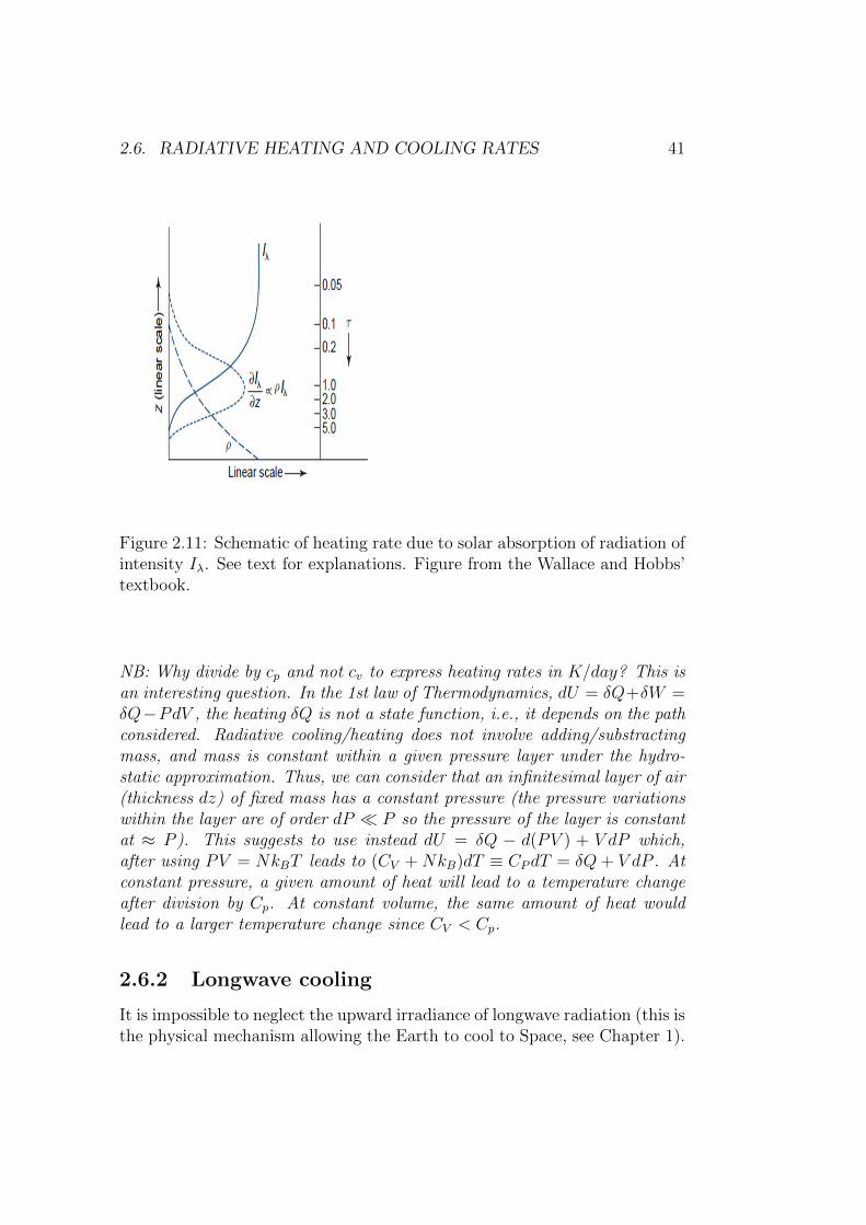
in which we have used (2.22). Fig. 2.11 gives a schematic of the verticalvariations of F ↓λ and ρqa = ρa, as well as a scale for the optical depth.The downward radiation decreases monotonically as we go downward, asexpected, and the density of absorber is assumed to be exponential-like.As can be seen, Qλ, the product of these two2, peaks at a height wherethe optical depth is close to unity. Physically, well above the level of unitoptical depth, the incoming beam is virtually undepleted, but the density isso low that there are too few molecules to produce significant absorption andheating. Likewise, well below the level of unit optical depth, there are a lotof molecules to produce absorption and heating, but there is not much leftto absorb as the beam has been mostly depleted. You are invited to provethis result mathematically in Q5 below.
Detailed calculations, using a “line-by-line radiation code” and includingthe contribution to Qλ from F ↑λ , are shown in Fig. 2.12 (focus here on theright hand side, i.e., shortwave heating rates). The heating rates are given inunits of K/day, i.e., Qλ/(ρcp) is plotted rather than Qλ. Absorption by ozonein the stratosphere dominates the heating rate, on the order of 5−10K/day.After this and O2 at high altitude (above the mesopause), the next mostimportant absorber of solar radiation is water vapour, which contributes toa relatively uniform heating of the troposphere on the order of 0.5K/day.
2We are neglecting here the temperature and pressure dependence of kλ.
2.6. RADIATIVE HEATING AND COOLING RATES 41
Figure 2.11: Schematic of heating rate due to solar absorption of radiation ofintensity Iλ. See text for explanations. Figure from the Wallace and Hobbs’textbook.
NB: Why divide by cp and not cv to express heating rates in K/day? This isan interesting question. In the 1st law of Thermodynamics, dU = δQ+δW =δQ−PdV , the heating δQ is not a state function, i.e., it depends on the pathconsidered. Radiative cooling/heating does not involve adding/substractingmass, and mass is constant within a given pressure layer under the hydro-static approximation. Thus, we can consider that an infinitesimal layer of air(thickness dz) of fixed mass has a constant pressure (the pressure variationswithin the layer are of order dP P so the pressure of the layer is constantat ≈ P ). This suggests to use instead dU = δQ − d(PV ) + V dP which,after using PV = NkBT leads to (CV +NkB)dT ≡ CPdT = δQ+ V dP . Atconstant pressure, a given amount of heat will lead to a temperature changeafter division by Cp. At constant volume, the same amount of heat wouldlead to a larger temperature change since CV < Cp.
2.6.2 Longwave cooling
It is impossible to neglect the upward irradiance of longwave radiation (this isthe physical mechanism allowing the Earth to cool to Space, see Chapter 1).

42CHAPTER 2. RADIATIVE HEATING AND COOLINGOF THE ATMOSPHERE
Figure 2.12: Global mean longwave (left panel) and shortwave (right panel)heating rates in K/day as a function of altitude showing contributions of themajor gases. After D. Andrews’ textbook.

2.6. RADIATIVE HEATING AND COOLING RATES 43
Nor is it possible to neglect the downward infrared irradiance responsible forthe greenhouse effect. We’ll thus compute both terms in this section. Besidesthis, the other important difference between the calculation here and that inthe previous section regards the transformation from Iλ to Fλ. As illustratedin fig. 2.13 this simply reflects the well defined source of shortwave radia-tion (the Sun) as opposed to the more diffuse sources of longwave radiation(Earth’s surface, atmospheric molecules, clouds, etc). Note that the differentpencils in Fig. 2.13 have also different path lengths. To treat this effectexplicitely without enhancing the complexity too much we’ll use the “par-allel plane approximation”, which treats the atmosphere as homogeneous inthe horizontal direction: one can then use for all pencils the optical thicknessmeasured along the direction z, after taking into account the increase in pathlength by the factor 1/ cos θ (see Fig. 2.13).
In the calculations below we’ll neglect scattering of longwave radiationand will accordingly use Jλ = Bλ (section 2.4.2) in Schwarzchild equation,i.e.,
Iλ(s) = Iλ(so)e−τ +
∫ τ
0
Bλ(τ′)e−(τ−τ
′)dτ ′ (2.44)
with τ = τλ(so, s) and τ ′ = τλ(so, s′).
Upward irradiance
Let’s first consider the contribution to F ↑λ arising from emission by the Earth’s
surface, i.e., the term corresponding to I↑λ(so) = Bλ(Ts) where Ts is theEarth’s surface temperature. Taking into account the 1/ cos θ term, the con-tribution F ↑λ,surf to the upward irradiance from the Earth’s surface is,
F ↑λ,surf (z) =
∫ 2π
0
Bλ(Ts)e−τ(z)/ cos θ cos θdΩ (2.45)
in which τ(z) = τλ(0, z) now measures the optical depth of the air columnfrom the surface to height z, and θ is the angle made by each pencil ofradiation with the vertical. Consistent with the parallel plane approximation,we assume that Ts does not vary too much, which allows us to take the Bλ(Ts)term outside the integral. After doing this, and introducing µ = cos θ, wehave,
F ↑λ,surf (z) = 2πBλ(Ts)
∫ 1
0
e−τ(z)/µµdµ (2.46)
A useful approximation is that 2∫ 1
0e−τ/µµdµ ≈ e−τ/ cos(53
) = e−1.66τ (“diffuseapproximation”). As a result,
F ↑λ,surf (z) ≈ πBλ(Ts)e−1.66τ(z) (2.47)

44CHAPTER 2. RADIATIVE HEATING AND COOLINGOF THE ATMOSPHERE
Figure 2.13: Schematic of the “radiation pencils” to be considered when com-puting irradiances at point P for the shortwave (left) and longwave (right)part of the spectrum. In absence of scattering, only one radiation pencil (theone covering the small solid angle δΩ subtented by the Sun) would need tobe considered for the shortwave part of the spectrum –but many need tobe taken into account for infrared radiation. The distance ds along a pathmaking an angle θ with the vertical is related to dz by ds = dz/ cos θ, hencethe factor 1/ cos θ in the calculations in this section.
2.6. RADIATIVE HEATING AND COOLING RATES 45
The total upward irradiance at z is then,
F ↑λ (z) ≈ πBλ(Ts)e−1.66τ(z) + F ↑λ,lay(z) (2.48)
where the second term on the r.h.s is the contribution of the atmosphericlower hemisphere (or layer), to the irradiance. Let’s see how we would esti-mate it if we were climate modellers, equipped with a (fast) computer. Fora given direction, i.e. a given slanted path, we would calculate the integralterm on the r.h.s of (2.44). Because of the plane parallel approximation,the result will not depend on the azimuthal direction, but only on z and θ.Writing it as Φ↑(z, θ),
Φ↑(z, θ) ≡∫ τ(z)/ cos θ
0
B(τ ′)eτ′dτ ′ (2.49)
where τ ′ measures the optical depth along the slanted path, the contributionof the atmospheric layer to the total irradiance would then be,
F ↑λ,lay(z) = 2π
∫ 1
0
Φ↑(z, µ)e−τ(z)/µµdµ. (2.50)
Downward irradiance
Because of the negligible amount of photons emitted by the Sun at wavelength≥ 4µm, the “surface term” for downward infrared radiation can be set to zero.Hence the downward irradiance at a height z only reflects the emission fromthe atmospheric column sandwiched between the “top-of-the-atmosphere”and z. The result would thus simply be the analog of (2.50) for downwardrather than upward integration. We can simply use the previous result andwrite,
F ↓λ (z) = F ↓λ,lay(z) = 2π
∫ 1
0
Φ↓(z, µ)e−τ(z)/µµdµ. (2.51)
in which τ(z) = τλ(TOA, z) is now the optical depth measured downwardfrom the “top-of-the-atmosphere”.
An illustration of the calculation is provided using the result in section2.5.2 for an isothermal atmosphere at T = To. Based on this the result, thedownward irradiance is,
F ↓λ (z) = 2π
∫ 1
0
Bλ(To)(1− e−τλ(z)/µ)µdµ ≈ πBλ(To)(1− e−1.66τλ(z)). (2.52)
The contribution of this irradiance to the heating rate can then be estimatedfrom (2.36) and an illustration is provided in Fig. 2.14 for an idealised water

46CHAPTER 2. RADIATIVE HEATING AND COOLINGOF THE ATMOSPHERE
Figure 2.14: A simple calculation of radiative cooling due to water vapour foran isothermal atmosphere at T = To = 255K. The specific humidity is takenas qa = 0.005e−z/3km and the background density is taken as ρ = 1.2e−z/8km.An extinction coefficient kλ = 0.03m2/kg was used over the 5µm ≤ λ ≤50µm. The heating rate (integrated over λ, in K/day) is displayed as afunction of height, as are the optical depth and associated transmissivity.The Matlab code is available on Blackboard.
vapour profile (i.e., the calculation assumes an exponential qa and a broadrange of wavenumbers –see caption). A mid-tropospheric peak in cooling ispredicted, with a magnitude on the order of 1K/day. The formula can alsobe applied for a “CO2 case” by making the mixing ratio qa uniform as afunction of height, by narrowing the range of wavenumbers and increasingthe opacity in that range. As seen in Fig. 2.15, the peak of cooling now movesupward, with very little cooling below 5km (this is because the irradiance is“saturated” at these levels and so does not vary with height).
Realistic numerical calculations of upward (red), downward (blue) and thenet (upward-downward, green) are shown in Fig. 2.16. These were carriedout for typical summertime conditions over the Northern Hemisphere (onlythree infrared absorbers were included, water vapour, carbon dioxide and
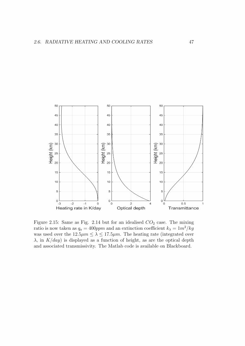
2.6. RADIATIVE HEATING AND COOLING RATES 47
Figure 2.15: Same as Fig. 2.14 but for an idealised CO2 case. The mixingratio is now taken as qa = 400ppm and an extinction coefficient kλ = 1m2/kgwas used over the 12.5µm ≤ λ ≤ 17.5µm. The heating rate (integrated overλ, in K/day) is displayed as a function of height, as are the optical depthand associated transmissivity. The Matlab code is available on Blackboard.

48CHAPTER 2. RADIATIVE HEATING AND COOLINGOF THE ATMOSPHERE
Figure 2.16: Calculations of upward (red), downward (blue) and net (green)irradiances for summertime conditions in the Northern Hemisphere. Cour-tesy of Wenyi Zhong and Jo Haigh from the SPAT group. The data and theMatlab code used to generate the plot are available on Blackboard.
ozone). Note that the irradiances are integrated over all wavelengths and aredisplayed as a function of pressure. The general shape is that of decreasingintensity as one goes up in the atmosphere for the upward irradiance: theupward infrared radiation is absorbed in the atmosphere and is re-emittedless strongly at upper (lower temperature, lower number density) than atlow levels (high temperature, high number density). Conversely, the generalshape for the downward irradiance is that of increase as one goes to lowerlevels: downward infrared is more effectively emitted at low levels where thetemperature and the number density are higher.
Heating rate
The net heating rates will reflect the competition between heating due to ab-sorption of the radiation emitted by other atmospheric layers and the ground,and the cooling due to the emission of longwave radiation. Detailed calcula-tions of the resulting heating rates, integrated over wavelengths, are shown inFig. 2.12 (left panel). The first thing to note is that, except for O3 near 25km,longwave heating rates are negative, on the order of several K/day. Infraredradiation thus cools the atmosphere globally, which opposes the heating due

2.6. RADIATIVE HEATING AND COOLING RATES 49
to absorption of shortwave radiation (previous subsection). Inspection ofFig. 2.16 suggests that the cooling reflects the fact that downward irradi-ance (blue curve) diverges more (i.e., cools atmospheric layers) than upwardirradiance (red curve) converges (i.e., heats atmospheric layers).
The primary reason why net cooling is found in the infrared is that theradiation that a given atmospheric layer exchanges with the ground andother layers tend to cancel out, but there is no cancellation when it comesto exchange of radiation with Space. Restating the arguments first put for-ward in Chapter 1 (Fig. 1.7), a given atmospheric layer emits upwards anddownwards towards layers above and below, but it also receives radiationfrom them. Likewise, it emits towards the Earth’s surface but also receivesupwards radiation from the Earth’s surface. Each of these exchanges approx-imately cancel out. In addition, the atmospheric layer in question also emitsinfrared radiation to Space but it does not receive such radiation in return.Hence a net cooling is expected, the so-called “cooling to Space” approxi-mation (clearly visible in Fig.2.16 as the increase of the green curve towardslower pressure). As Fig. 2.12 shows, this is mostly due to water vapour inthe troposphere, and carbon dioxide in the stratosphere and the mesosphere.
2.6.3 Net radiative heating rates
The compensation between infrared cooling and shortwave heating is imper-fect in the troposphere, where a net cooling of about 1K/day is suggested inFig. 2.12. This is expected since the troposphere receives energy from theoceans and the land (heat and moisture exchange). Likewise in the meso-sphere (height above ≈ 50km in Fig. 2.12) a net radiative heating is sug-gested (this is opposed by molecular diffusion of heat upward at these levels–the density of air is so small there that molecular diffusion becomes a majorplayer in the heat budget). In the stratosphere however the compensationbetween infrared cooling and shortwave heating is good: the stratosphere isclose to a radiative equilibrium.
One way to visualize this competition is proposed in Fig. 2.17. In theright panel is shown the downward net shortwave flux: largest at the TOAand decreasing slighty towards the Earth’s surface as a result of absorptionby atmospheric gases, aerosols and clouds. On the left panel is shown thenet longwave flux, which is upward at all levels: at the TOA it must benearly equal in length to the solar flux since the Earth is approximatively inradiative balance. At the surface its length must be less than the downwardsolar flux since the Earth’s surface itself is in equilibrium and cools by surfaceevaporation and heat transfer, in addition to emitting infrared radiation. Ata given level, the air cools through radiative exchanges in the infrared (the
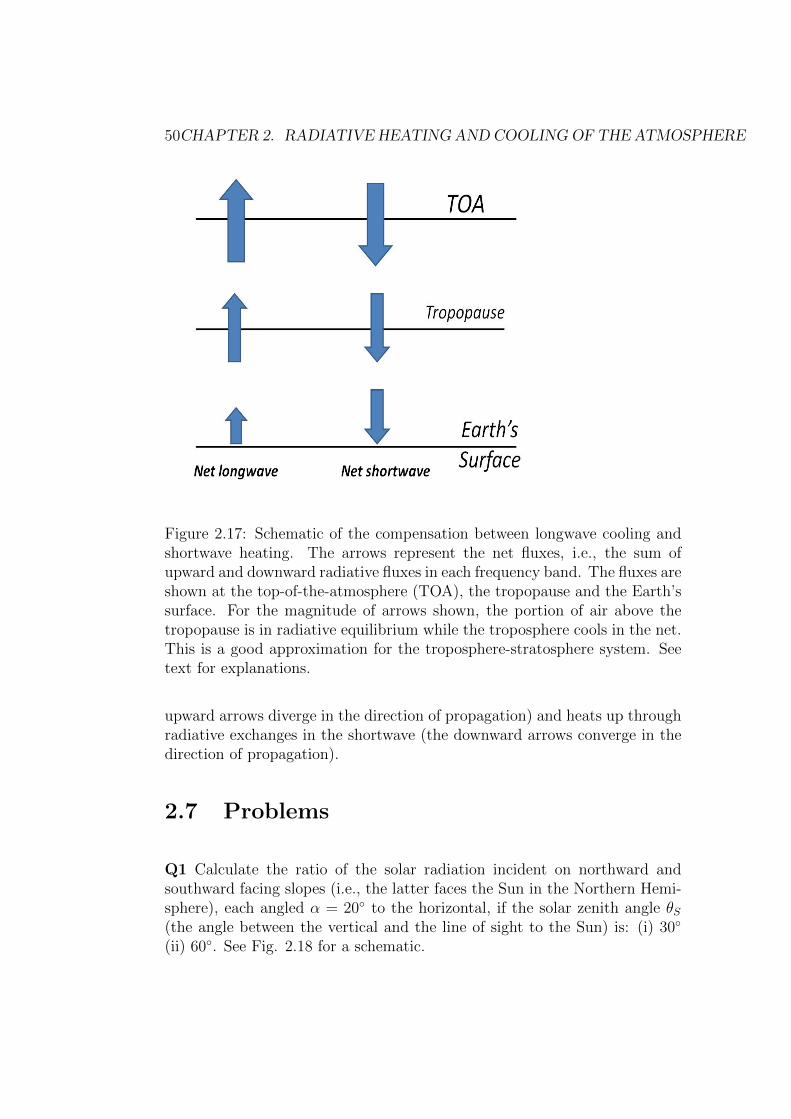
50CHAPTER 2. RADIATIVE HEATING AND COOLINGOF THE ATMOSPHERE
Figure 2.17: Schematic of the compensation between longwave cooling andshortwave heating. The arrows represent the net fluxes, i.e., the sum ofupward and downward radiative fluxes in each frequency band. The fluxes areshown at the top-of-the-atmosphere (TOA), the tropopause and the Earth’ssurface. For the magnitude of arrows shown, the portion of air above thetropopause is in radiative equilibrium while the troposphere cools in the net.This is a good approximation for the troposphere-stratosphere system. Seetext for explanations.
upward arrows diverge in the direction of propagation) and heats up throughradiative exchanges in the shortwave (the downward arrows converge in thedirection of propagation).
2.7 Problems
Q1 Calculate the ratio of the solar radiation incident on northward andsouthward facing slopes (i.e., the latter faces the Sun in the Northern Hemi-sphere), each angled α = 20 to the horizontal, if the solar zenith angle θS(the angle between the vertical and the line of sight to the Sun) is: (i) 30
(ii) 60. See Fig. 2.18 for a schematic.

2.7. PROBLEMS 51
Figure 2.18: Geometry for Q1.
Q2 Calculate the intensity I of solar radiation at the top-of-the-atmosphere(TOA), given the irradiance F = 1361Wm−2 at zero zenith angle. The radiusof the Sun is Rs = 7×10⁸m while the Earth-Sun distance is d = 1.5×10¹¹m.
Q3 Consider monochromatic radiation passing through a gas with absorptioncoefficient βλ = 0.01m2kg−1. (i) What fraction of the beam is absorbed inpassing through a layer containing 1kgm−2 of the gas? (ii) What mass perunit area would the gas layer have to have in order to absorb half the incidentradiation?
Q4 Suppose the gas in the previous question is present with uniform massmixing ration q = 10−3 in an atmosphere in hydrostatic equilibrium. Takesurface pressure to be Ps = 1000hPa. (i) Show that the optical depth mea-sured from the top of the atmosphere is linearly proportional to pressure.What is the constant of proportionality? (ii) Estimate the pressure of thelevel that is one optical depth from the top of the atmosphere.
Q5 Show that, for a beam of monochromatic solar radiation Fλ incident

52CHAPTER 2. RADIATIVE HEATING AND COOLINGOF THE ATMOSPHERE
vertically on an atmosphere in which the mixing ratio of the radiativelyactive gas is independent of height and the density decreases exponentiallywith height, the heating rate per unit volume is greatest at unit optical depth.
Q6 Show that, for the situation in the previous question, the heating rateper unit mass is greatest near the top of the atmosphere.
Q7 Now consider infrared radiation traveling upwards (optical depth mea-sured from Earth’s surface) in an atmosphere where the total optical depthat the wavelength of the radiation considered is τ∞ = 5. (i) What fraction ofthe monochromatic intensity emitted by the ground is absorbed in passingthrough the layer of atmosphere extending from optical depth 0.2 to 4.0?(ii) What fraction of the intensity emitted to space is emitted by the layerbetween 0.2 and 4.0 optical depth? You may assume the atmosphere to beisothermal for this part, and at the same temperature as the Earth’s surface.
Q8 Past exam question (2005, No 3).
(i) Derive an expression for the emission (or effective) temperature of theEarth as a function of solar constant and albedo.
(ii) Estimate numerically the sensitivity of the effective temperature to fluc-tuations in albedo. (Solar constant So = 1370Wm−2, planetary albedoαP = 0.3 and Stefan-Boltzmann constant σ = 5.67× 10⁻⁸Wm−2K−4).
(iii) Over the last 10 years the global mean temperature has risen by about0.2C. If clouds have an albedo of 0.8 and the surface has an albedo of0.1, what change in the cloud percentage cover could account for thistemperature rise? State any assumption you make.
(iv) If the transmissivity of clouds increased by 10 % but the cloud coverstayed the same what would the new equilibrium temperature be?
(v) Why is the observed surface temperature larger than the effective tem-perature?
(vi) In which direction must the observed net radiation at the surface beand why?
Q9 Figure 2.19 shows an estimate of the flux of solar radiation impinging onthe Earth (the solar constant So). Show that it is in good agreement with apen and paper prediction assuming only knowledge of the radius of the Sun

2.7. PROBLEMS 53
Figure 2.19: Composite measurement of the Solar “constant” So from Spacethrough time (in Wm−2). From Joanna Haigh’s briefing paper published bythe Grantham Institute for Climate Change at Imperial College in 2011.
rsun = 6.96× 10⁸m, the Sun’s emission temperature Tsun = 5780K, and themean Earth-Sun distance d = 1AU = 1.5× 10¹¹m.
Q10 A sunphotometer is an instrument designed to measure the opticalthickness of the atmosphere due to scattering and absorption of solar radia-tion by air molecules and aerosols. At the ground, two measurements of theincident solar radiation at a wavelength λ = 1µm, denoted by Iλ, are made.These are made at two different solar zenith angles θ1 = 20 and θ2 = 40.
(i) Show that the ratio rλ = (Iλ)1/(Iλ)2 of the two intensities satisfy,
ln rλ = τλ(sec θ2 − sec θ1) (2.53)
in which τλ =∫ +∞0
kλρqadz is the “column” optical depth.
(ii) The ratio of the two intensity measurements is rλ = 1.12. Compute thecolumn’s optical depth using the data above, stating any assumptionsmade.

54CHAPTER 2. RADIATIVE HEATING AND COOLINGOF THE ATMOSPHERE

Chapter 3
Radiative-convectiveequilibrium
Key concepts: radiative equilibrium, fluid parcel, environment, buoyancy,Brunt-Vaisala frequency, radiative-convective equilibrium.
The preceding chapters showed that the atmosphere cools through (net)radiative processes (Chapter 2) and is heated from below through surfaceevaporation and sensible heat fluxes (Chapter 1). This situation destabilizesthe atmosphere because, at same pressure warm air is lighter than cold air,and thus rises, while cold air sinks. The effect is to generate a convectivecell which restores the equilibrium by carrying heat upward. In this chapterwe study simple models of this interaction between radiation (destabilizing)and convection (stabilizing).
3.1 Radiative equilibrium
Mathematically, the state of radiative equilibrium is such that the net ra-diative heating (i.e., the sum of shortwave and longwave parts) is zero at allheights. Using the result from Chapter 2, this reads,
Qrad =
∫ +∞
0
Qλdλ =d
dz
∫ +∞
0
(F ↓λ − F↑λ )dλ = 0 (for all z) (3.1)
Since the longwave emission depends on temperature, there must be a par-ticular choice of this variable allowing (3.1) to be satisfied. It is referred toas the “radiative equilibrium” temperature.
Figure 3.1 (left panel) provides an example of a radiative equilibriumtemperature calculation. The input for such calculation is the distribution
55

56 CHAPTER 3. RADIATIVE-CONVECTIVE EQUILIBRIUM
Figure 3.1: Approach to radiative (left) and radiative-convective (right) equi-librium in a time dependent caculation (Manabe and Strickler, 1964). Eachcurve represents temperature (x-axis) vs pressure (y-axis). Dashed curvesrefer to a cold start while continuous lines refer to a warm start. The thicklines indicate the equilibrium temperature profile in each case. In the rightpanel, they also locate the region of minimum temperature, the model’s“tropopause”.
of radiatively active constituents as a function of height, and the incidentsolar radiation at the TOA. (note that in this example, clouds were omittedand water vapour as well as ozone and carbon dioxide distributions werespecified). When starting for example from a cold isothermal state at T =160K (dashed lines), one observes a systematic warming at all levels as timeincreases, reaching a steady state after about 300 days (thick continuouscurve). This warming is pronounced near the surface and at upper levels.Note that the same equilibrium is reached if one starts from a warm stateT = 360K (continuous lines).
What happens in these experiments is that the shortwave part of the heat-ing rate is essentially fixed (it does not depend on temperature). The long-wave cooling, however strongly depends on temperature through Schwarzchild’sequation (Chapter 2). In the cold start for example, a given layer of air doesnot emit enough longwave radiation to offset the shortwave heat gain and,

3.2. CONVECTION 57
as a result, it warms. By warming up, it emits more in the infrared (theblackbody radiation term in Schwarzchild’ equation) and so the net warmingdecreases. When the equilibrium temperature is reached, the layer cools asmuch by infrared than it gains heat from shortwave absorption. No furthertemperature change can arise.
An interesting feature of Fig. 3.1 is that it displays the time evolutionof the temperature profile. Whether starting from a cold or a warm state,it takes several months to reach the final equilibrium temperature profile.This suggests that atmospheric motions such as weather disturbances, con-vective cloud systems, and others, can be considered as adiabatic since theirtimescale is much shorter than a few months.
3.2 Convection
If we were to perturb slightly the radiative temperature equilibrium, say byallowing a small upward velocity at low level, and wait long enough, wouldthe same temperature profile be found? In other words, is the radiative tem-perature equilibrium stable to “dynamical” as opposed to thermal changes?
Unfortunately, the answer is a clear no, and this is the main reason whyweather and climate predictions are difficult to make! The radiative temper-ature profile is not stable to displacements of the layers: convective motionwill develop and change the final temperature. We first study the basicsof this instability and return to the problem of the radiative temperatureequilibrium later in the chapter.
3.2.1 The “parcel’s equation”
The key concept to understand convection is that of buoyancy whom youmight remember from Archimede’s principle. In Atmospheric sciences thisconcept is tied to that of an air parcel, a small enough sample of air thatit describes locally what happens in the atmosphere, but made of a largeenough number of molecules that we can apply thermodynamics to it.
Consider such parcel initially at a reference height zo in the atmosphere.We ignore horizontal variations. From Newton’s second law, the motion ofthe parcel obeys,
dwpdt
=∑i
Fi (3.2)
where Fi refers to any force per unit mass acting on the parcel of upwardvelocity wp. The forces in question here are simple gravity and the pressure
58 CHAPTER 3. RADIATIVE-CONVECTIVE EQUILIBRIUM
gradient force,dwpdt
= −g − αpdP
dz(3.3)
in which αp is the volume per unit mass (or specific volume) of the parceland P is the pressure. We wish to establish whether, once displaced initially,the parcel will come back to zo (stable case) or move away from it (unstablecase).
We will carry out a thorough investigation of all the forces acting on a parcelof air in chapter 4 (including Coriolis and centrifugal forces, as well as trans-port of momentum by the flow). As it turns out, the approximation (3.3)will be shown to be accurate.
The key concept to answer this question is that of the “environment”,i.e., the atmosphere before we displaced the parcel. In the question at hand(stability of the radiative equilibrium state), the environment is simply a stateof rest (no motion) with the temperature equal to the radiative equilibriumtemperature. The environment (subscript e) thus satisfies,
0 = −g − αedPedz
(3.4)
Note that this equilibrium is the “hydrostatic balance” (1.8) introduced inChapter 1.
To make further predictions regarding the parcel’s fate, we will make twoassumptions:
(i) the pressure field is not modified by the parcel’s motion, so the P in(3.3) and in (3.4) are equal
(ii) the parcel does not acquire any heat as it moves (consistent with theshort timescale of this process compared to radiative processes, see Fig.3.1) and the ascent does not involve irreversibilities such as mixing withsurrounding air, friction, etc. As a result the entropy of the parcel isconserved during the ascent (second law of Thermodynamics).
As a result of (i), we can rewrite (3.3) as,
dwpdt
= g(αp − αe)
αe(3.5)
This equation shows that if the specific volume of the parcel is greaterthan that of the environment, the parcel will exhibit upward acceleration(dwp/dt > 0). Likewise, if the parcel has a smaller specific volume than the
3.2. CONVECTION 59
environment, it will be accelerated downwards. The r.h.s in (3.5) is calledthe buoyancy force B,
B = g(αp − αe)
αe(3.6)
3.2.2 Potential temperature
Up to now the derivation has been fairly general. We restrict from now onthe discussion to the case of dry air so that the pressure P = Pd and theequation of state for the parcel is simply the ideal gas law Pdαd = RdT (seeChapter 1). This allows to rewrite (3.5) as1,
dwPdt
= −g (Te − Tp)Te
(3.7)
The goal of this subsection is to introduce a quantity called “potential tem-perature”, which is going to allow us to solve (3.7) by using the secondassumption above (isentropic ascent).
Potential temperature is simply meteorologist’s jargon for entropy. Theconcept is best illustated with the following calculation. Consider an airparcel at upper levels where its temperature is T and its pressure is P .Suppose we bring this parcel adiabatically to the surface where the pressureis Pref = 1000hPa. What would be its new temperature? We’ll call thelatter potential temperature, with the variable θ, to express that it is thetemperature an air parcel at T, P would have if it were brought adiabaticallyto the surface.
To find a formula for θ, use that in an adiabatic process, entropy isconserved. For dry air, this reads,
cp,ddT/T −RddP/P = 0 (3.8)
since the specific entropy of dry air is sd = cp,d lnT − Rd lnP (in this ex-pression cp,d is the specific heat capacity at constant pressure). This can beintegrated from P to Pref and T to θ,∫ T
θ
dT/T =Rd
cp,d
∫ P
Pref
dP/P, (3.9)
1In doing so one must neglect the difference between the pressure of the parcel (Pp) andthat (Pe) of the environment: otherwise the ratio of specific volumes αp/αe would includea term Pp/Pe. It can be shown that this is valid as long as the velocity of the parcel isless than the speed of sound, which is valid for the atmospheric applications consideredhere (i.e., Pp ≈ Pe for the motions considered in this course).
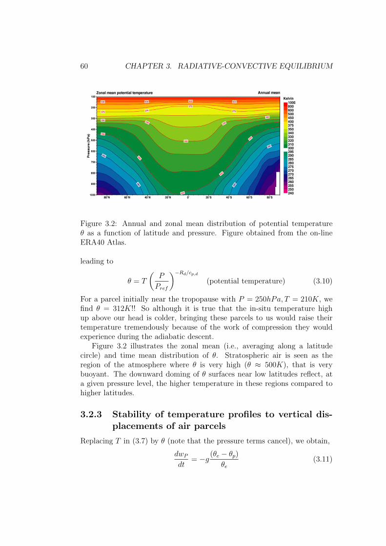
60 CHAPTER 3. RADIATIVE-CONVECTIVE EQUILIBRIUM
Figure 3.2: Annual and zonal mean distribution of potential temperatureθ as a function of latitude and pressure. Figure obtained from the on-lineERA40 Atlas.
leading to
θ = T
(P
Pref
)−Rd/cp,d(potential temperature) (3.10)
For a parcel initially near the tropopause with P = 250hPa, T = 210K, wefind θ = 312K!! So although it is true that the in-situ temperature highup above our head is colder, bringing these parcels to us would raise theirtemperature tremendously because of the work of compression they wouldexperience during the adiabatic descent.
Figure 3.2 illustrates the zonal mean (i.e., averaging along a latitudecircle) and time mean distribution of θ. Stratospheric air is seen as theregion of the atmosphere where θ is very high (θ ≈ 500K), that is verybuoyant. The downward doming of θ surfaces near low latitudes reflect, ata given pressure level, the higher temperature in these regions compared tohigher latitudes.
3.2.3 Stability of temperature profiles to vertical dis-placements of air parcels
Replacing T in (3.7) by θ (note that the pressure terms cancel), we obtain,
dwPdt
= −g (θe − θp)θe
(3.11)

3.2. CONVECTION 61
At first sight, not much is gained. Upon reflection though we see that wehave replaced T , a non conserved variable during the ascent, by θ which isconserved (you can easily check that ds = 0 implies dθ = 0). In particular,if we start the parcel at zo with the same temperature as the environment,θp(zo) = θe(zo) while at z, θe(z) = θe(zo) + dθe/dz(z − zo). This shows that,since the parcel conserves its entropy during the ascent, i.e., θp(z) = θp(zo),
d2(zp − zo)dt2
+g
θe
dθedz
(zp − zo) = 0 (3.12)
in which we have used wp = dzp/dt, zp being the height of the parcel.This equation shows that the fate of the parcel is governed by the sign of
the quantity N2, defined as,
N2 ≡ g
θe
dθedz
(the Brunt-Vaisala frequency) (3.13)
When N2 > 0, (3.12) is an harmonic oscillator with angular frequency N :the parcel undergoes stable oscillations around z = zo. When N2 < 0, theparcel displacement is unstable: if initially displaced upwards, it will keepgoing upwards, being constantly accelerated upwards by the buoyancy force(and likewise if initially displaced downwards, the parcel will keep acceler-ating downwards). The Brunt-Vaisala frequency is clearly a very importantvariable describing the atmosphere (see section 3.5).
A couple of important comments:
(i) From Fig. 3.2 we see that the atmosphere has, in the mean, N2 > 0.So it is stable to vertical displacements of air parcels.
(ii) From the plot, one can estimate roughly that N = [(9.81/315)× (330−300)/5km]1/2 ' 10−2s−1. This corresponds to a period of oscillation ofabout 10 minutes.
(iii) The fact that the time mean and zonal mean picture has N2 > 0 doesnot mean that the atmosphere is always everywhere, and at all times,stable. Indeed the deep anvil clouds that one sometimes experienceson a summer day (Fig. 3.3) are the manifestation of a region of N2 <0. This arose because parcels at low levels increased their entropytremendously through heating with the hot Earth’s surface while, aloft,they cooled through infrared radiation. This state of affair generateshigh θp at low levels and low θe at upper level and thus a positivebuoyancy for air parcels from (3.11). NB: clearly moisture effects mustbe invoked to discuss this aspect fully, and this is postponed to section3.4.

62 CHAPTER 3. RADIATIVE-CONVECTIVE EQUILIBRIUM
Figure 3.3: An intense “anvil cloud”. Surface heating throughout the dayincreased the entropy of air parcels at low levels while infrared radiativecooling decreased that of air parcels at upper levels (this latter effect isadmittedly weaker than the heating due to heat exchange with the Earth’ssurface). Note that air parcels seem “stuck” at the top and spread laterally.This reflects that even though they acquire large buoyancy through surfaceheating, this buoyancy was still less than that of the environmental air atupper levels (the tropopause here). Thus in this example the spreading allowsyou to “see” the tropopause!
3.3. RADIATIVE-CONVECTIVE EQUILIBRIUM 63
3.3 Radiative-convective equilibrium
3.3.1 Stability of the radiative equilibrium tempera-ture profile
We now return to Fig. 3.1 (left column) and the stability of the radiativetemperature equilibrium. At the surface, the temperature is T ≈ 330K witha pressure P = 1000hPa. Higher up, there is a minimum temperature ofabout 180K, reached at a pressure ≈ 300hPa. Application of (3.10) withPref = 1000hPa shows that the surface potential temperature is 330K whileat 300hPa it is ≈ 254K. Hence θ decreases with height (N2 < 0) and theradiative equilibrium temperature profile is unstable!
What this says is that radiative processes destabilize the atmosphere andthat consideration of radiation only cannot provide a realistic prediction forthe temperature structure of the atmosphere. The right panel in Fig. 3.1is an attempt to represent the effect of convection, by bringing artificiallythe atmosphere into a state with N2 = 0 (i.e., neutral to vertical displace-ments of air parcels –see section 3.4.2 below). Independently of the typeof convective parameterization used, we will refer to this state as one ofradiative-convective equilibrium.
The radiative - convective equilibrium state has a weaker change of tem-perature with height, i.e., a weaker “lapse-rate” Γ in the right compared tothe left panel,
Γ ≡ −dTdz
(definition of lapse-rate) (3.14)
It also has colder surface temperature (about 290K), and higher temperaturealoft. This reflects that by carrying high θ parcels upwards and replacingthem by cold θ parcels going downward, convection carries heat upward.Denoting the associated heating rate per unit volume as Qconv, we extendthe mathematical definition of radiative equilibrium definition in eq. (3.1)to that of radiative-convective equilibrium:
Qrad +Qconv = 0 (“Radiative-convective” equilibrium) (3.15)
3.3.2 The Tropopause
An interesting feature in Fig. 3.1 is the presence of a clear discontinuityin the lapse-rate (from being positive to negative) around 300hPa. Thisdiscontinuity is very pronounced in the radiative equilibrium (left panel),with a sharp transition between the lower (Γ > 0) and upper atmosphere(Γ < 0). In the radiative - convective equilibrium state, the discontinuity

64 CHAPTER 3. RADIATIVE-CONVECTIVE EQUILIBRIUM
is still seen, but is less pronounced, the layer between 10 and 25km beingnearly isothermal (Γ ≈ 0).
Returning to Chapter 1 (Fig. 1.4), we identify this discontinuity in lapserate as the tropopause. The previous paragraph makes it clear that it arisesprimarily as a result of radiative constraints: the absence of significant ab-sorption of solar radiation below about 10km leads, in pure radiative equi-librium, to a region of positive lapse-rate (see the simple calculations in Q4below). Conversely, in a region where there is absorption of solar radiation,pure radiative equilibrium leads to negative lapse-rate (so that this regioncan cool by emitting more infrared radiation at its top than at its bottom).The “dynamics” (convective adjustment here) merely modulates the exactvalue of the height at which this transition happens.
Returning to Fig. 3.1, the fact that the two temperature profiles (left andright panels) differ below the tropopause is expected from the fact that theradiative calculation has N2 < 0 there. Above the tropopause, the radiativeequilibrium temperature is very stable (a region of Γ < 0 has a very largeN2), so no instability is expected and the difference between the two tem-perature profiles is more surprising. What we are seeing in action here is theinteraction of convection with radiation: changing the tropospheric temper-ature through convection affects the upward infrared radiation reaching thestratosphere, and thus perturbs radiative heating rates in this region. Thecalculation shows that above ≈ 25km this effect becomes negligible and theradiative and radiative-convective equilibrium temperature profiles are thesame.
3.4 Dynamical effects of moisture?
3.4.1 Dry and moist adiabatic lapse-rates
We have managed to get a long way by simply considering the buoyancy ofdry air. However, as a buoyant air parcel rises, its internal energy (temper-ature) decreases because of the work of expansion done by the parcel on thesurrounding air. As a result, phase change can occur. As we shall see, thelatent heat released at this stage increases significantly the buoyancy of theparcel. Thus, in addition to important radiative effects, moisture also playsa key role in the dynamics.
To isolate clearly this role we are going to consider the case of cloudy, asopposed to pure dry, air. We will restrict ourselves to a mixture of dry air,water vapour and liquid water, the two latter phases being in thermodynamicequilibrium. This means that the vapour pressure e is solely a function of
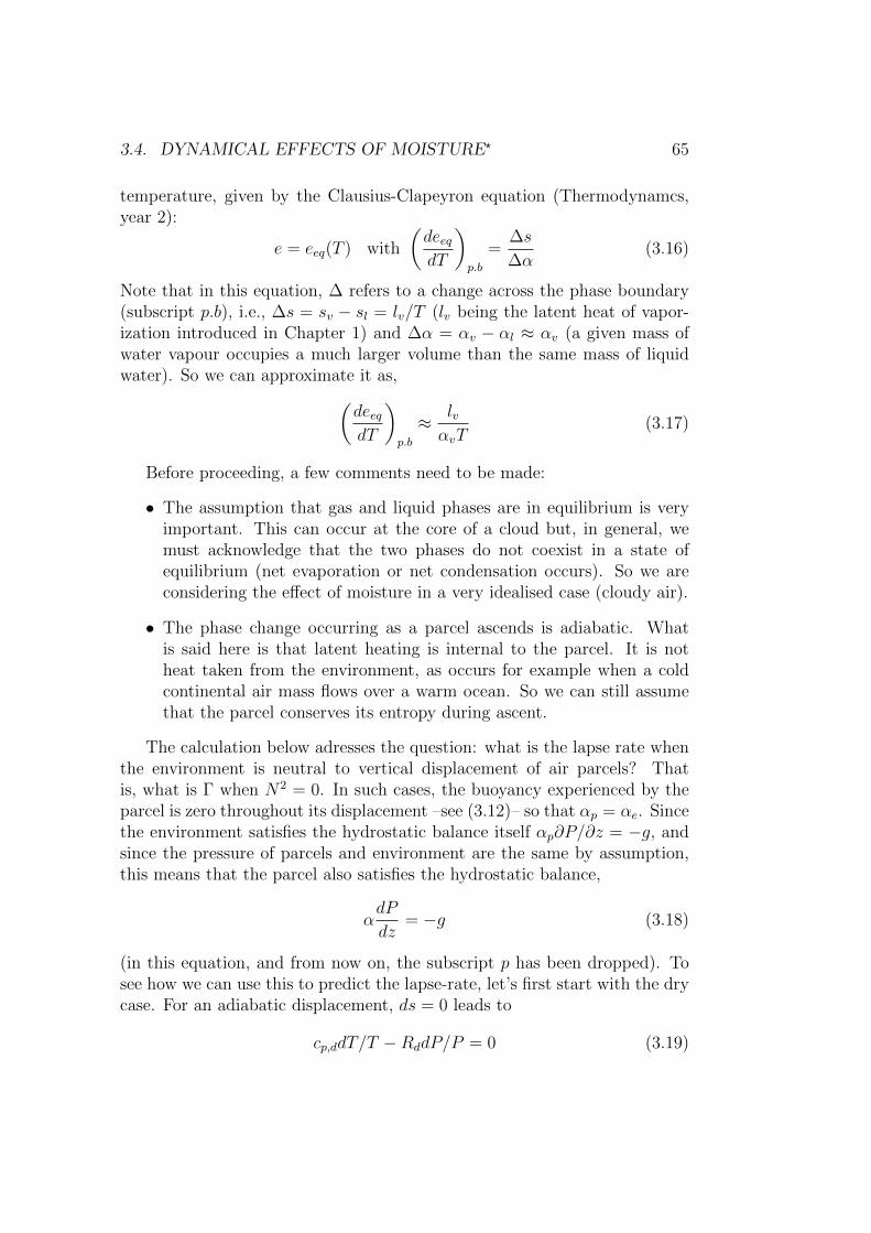
3.4. DYNAMICAL EFFECTS OF MOISTURE? 65
temperature, given by the Clausius-Clapeyron equation (Thermodynamcs,year 2):
e = eeq(T ) with
(deeqdT
)p.b
=∆s
∆α(3.16)
Note that in this equation, ∆ refers to a change across the phase boundary(subscript p.b), i.e., ∆s = sv − sl = lv/T (lv being the latent heat of vapor-ization introduced in Chapter 1) and ∆α = αv − αl ≈ αv (a given mass ofwater vapour occupies a much larger volume than the same mass of liquidwater). So we can approximate it as,(
deeqdT
)p.b
≈ lvαvT
(3.17)
Before proceeding, a few comments need to be made:
• The assumption that gas and liquid phases are in equilibrium is veryimportant. This can occur at the core of a cloud but, in general, wemust acknowledge that the two phases do not coexist in a state ofequilibrium (net evaporation or net condensation occurs). So we areconsidering the effect of moisture in a very idealised case (cloudy air).
• The phase change occurring as a parcel ascends is adiabatic. Whatis said here is that latent heating is internal to the parcel. It is notheat taken from the environment, as occurs for example when a coldcontinental air mass flows over a warm ocean. So we can still assumethat the parcel conserves its entropy during ascent.
The calculation below adresses the question: what is the lapse rate whenthe environment is neutral to vertical displacement of air parcels? Thatis, what is Γ when N2 = 0. In such cases, the buoyancy experienced by theparcel is zero throughout its displacement –see (3.12)– so that αp = αe. Sincethe environment satisfies the hydrostatic balance itself αp∂P/∂z = −g, andsince the pressure of parcels and environment are the same by assumption,this means that the parcel also satisfies the hydrostatic balance,
αdP
dz= −g (3.18)
(in this equation, and from now on, the subscript p has been dropped). Tosee how we can use this to predict the lapse-rate, let’s first start with the drycase. For an adiabatic displacement, ds = 0 leads to
cp,ddT/T −RddP/P = 0 (3.19)
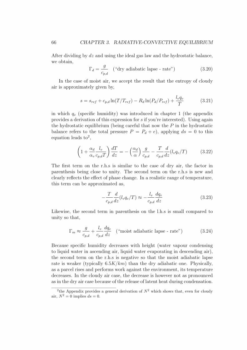
66 CHAPTER 3. RADIATIVE-CONVECTIVE EQUILIBRIUM
After dividing by dz and using the ideal gas law and the hydrostatic balance,we obtain,
Γd =g
cp,d(“dry adiabatic lapse - rate”) (3.20)
In the case of moist air, we accept the result that the entropy of cloudyair is approximately given by,
s = sref + cp,d ln(T/Tref )−Rd ln(Pd/Pref ) +lvqvT
(3.21)
in which qv (specific humidity) was introduced in chapter 1 (the appendixprovides a derivation of this expression for s if you’re interested). Using againthe hydrostatic equilibrium (being careful that now the P in the hydrostaticbalance refers to the total pressure P = Pd + e), applying ds = 0 to thisequation leads to2,(
1 +αdαv
lvcp,dT
)dT
dz= −
(αdα
) g
cp,d− T
cp,d
d
dz(lvqv/T ) (3.22)
The first term on the r.h.s is similar to the case of dry air, the factor inparenthesis being close to unity. The second term on the r.h.s is new andclearly reflects the effect of phase change. In a realistic range of temperature,this term can be approximated as,
− T
cp,d
d
dz(lvqv/T ) ≈ − lv
cp,d
dqvdz
(3.23)
Likewise, the second term in parenthesis on the l.h.s is small compared tounity so that,
Γm ≈g
cp,d+
lvcp,d
dqvdz
(“moist adiabatic lapse - rate”) (3.24)
Because specific humidity decreases with height (water vapour condensingto liquid water in ascending air, liquid water evaporating in descending air),the second term on the r.h.s is negative so that the moist adiabatic lapserate is weaker (typically 6.5K/km) than the dry adiabatic one. Physically,as a parcel rises and performs work against the environment, its temperaturedecreases. In the cloudy air case, the decrease is however not as pronouncedas in the dry air case because of the release of latent heat during condensation.
2the Appendix provides a general derivation of N2 which shows that, even for cloudyair, N2 = 0 implies ds = 0.

3.4. DYNAMICAL EFFECTS OF MOISTURE? 67
3.4.2 Application of “dry and moist adiabats thinking”
Parameterisation of convective instability
In either the dry or moist case, the state of neutrality to vertical displace-ment of air parcels is one in which no energy can be extracted from the“environment”, i.e., air parcels cannot gain kinetic energy through the workof buoyancy forces (identically zero). This is what motivates the param-eterisation of convection in Fig. 3.1 (right panel): radiation generates anunstable temperature profile but convection uses rapidly the energy storedin that profile to generate motions so that there is never any “left over” en-ergy available. Setting Γ to be equal to Γm in the calculation in Fig. 3.1(right panel), and thus imposing N2 = 0 throughout the calculation, is avery powerful and simple way to represent this state of affair.
Conditional instability
The calculations above for a dry and a cloudy parcel are exact when theenvironment is neutral (N2 = 0). When N2 6= 0, they would have to bemodified by replacing g by gαp/αe, since the parcel is now experiencing abuoyancy force3. This correction is small. For example, for dry air, αp/αe =θp/θe is at most 300± 10K/300K, i.e., a 3% error. Thus in practice, we canconsider that the temperature lapse rate of a dry parcel during its adiabaticdisplacement follows approximatively Γd. Likewise for a moist parcel andΓm. This is very useful, as the exemple below shows.
Consider the temperature profile in Fig. 3.4 (black), whose lapse rate Γis somewhere in between dry and moist adiabats (i.e., Γm ≤ Γ ≤ Γd). If wewere to lift an air parcel from the surface upward (for example as a resultof a large scale convergence of air near the surface), would it continue to goup? Here we take into account moisture and do not assume that the parcel isalready in equilibrium of phases (i.e., the relative humidity is less than unityat the surface).
Starting at the surface at A, we displace the parcel upward following adry adiabat since no liquid water is yet present4. For the case shown, this dis-placement is stable since the temperature decreases faster with height alonga dry adiabat (blue) than it does for the environment (black). Nevertheless,
3This is because we can only use αp∂P/∂z = −g when αp = αe since it is only theenvironment which is in hydrostatic balance when N2 6= 0.
4Some of you might rightly question the use of a dry adiabat for the isentropic ascentof a mixture of dry air and water vapour considered here. Doing the calculation properlywould only change the lapse rate slightly but would require using an exotic quantity called“virtual potential temperature”. For simplicity I decided not to do this.

68 CHAPTER 3. RADIATIVE-CONVECTIVE EQUILIBRIUM
Figure 3.4: An idealized temperature profile (black) with dry (blue) andmoist (green) adiabats superimposed. The LCL is the “lifting condensationlevel” where the temperature equals the dewpoint temperature (i.e., wherethe first drop of liquid water is produced by condensation). The LFC is the“level of free convection”, beyond which the parcel’s displacement would be-come unstable. In the lower panel, the trajectory of the sample is shown inthe temperature (T ) - vapour partial pressure (e) space. The displacementfrom A to B is on the vapour side of the phase diagram, and follows approx-imatively a line of constant e. From then on, the displacement is along thephase boundary (purple curve).

3.5. RADIATIVE-CONVECTIVE EQUILIBRIUMANDTHE REALWORLD69
at some point the temperature of the parcel has dropped enough that con-densation occurs. This happens at a temperature Td (dewpoint temperature)such that:
eeq(Td) = e (3.25)
in which eeq is the equilibrium vapor pressure (a function of temperature only,given by integration of the Clausius-Clapeyron equation –see eq. (3.16) insection 3.4.1) and e the vapor pressure in the sample. The level at which thisoccurs is called the “lifting condensation level” (point B in the figure). Fromthis point onward our sample is in thermodynamic equilibrium of phases (i.e.,the relative humidity is unity) so further adiabatic lifting will proceed alongthe moist adiabat (green curve). For the case shown, the parcel is still lessbuoyant than the surrounding from B to C, the latter being the point wherethe parcel’s temperature equals that of the environment. Thus the deplace-ment is overall stable from A to C. Beyond C however, the displacementis unstable, since the parcel’s temperature exceeds that of the environment(and its pressure equals that of the environment).
In summary, if the parcel has enough kinetic energy when it starts at thesurface, it could reach C at which point buoyancy forces will accelerate itfurther upward. This type of instability is called “conditional instability”.This situation occurs frequently in the atmosphere, and the LCL is readilyidentified as the cloud base. Deep convective clouds are those where enoughenergy was available at low levels to reach the LFC. We’ll return to theseideas in the lecture on clouds (powerpoint file on Blackboard).
3.5 Radiative-convective equilibrium and the
real world
The main message from all the above is that there is a competition betweenradiative processes, which tend to destabilize the atmosphere, and dynamicalprocesses, which tend to stabilize the atmosphere. The 1D case illustrated inFig. 3.1 showed that radiation acts relatively slowly (it took several monthsto achieve radiative equilibrium on the left panel). Convection is expected tobe much faster (a moderate updraft of 10cm/s would reach the tropopause intypically 10km/10cms−1 ≈ 1day). As a result, the prediction is that convec-tion should dominate and we do not expect to observe unstable temperatureprofiles.
Figure 3.5 displays the observed ratio (Γm−Γ)/Γm. It is clearly seen thatin the Tropics (equatorward of 30 of latitude), and above the near surfacelayer (P ≤ 900hPa), observed lapse rates are within 10 % of the moist adi-
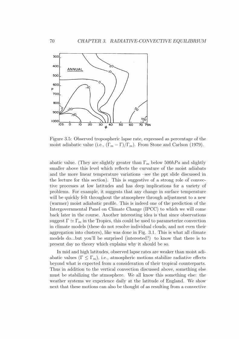
70 CHAPTER 3. RADIATIVE-CONVECTIVE EQUILIBRIUM
Figure 3.5: Observed tropospheric lapse rate, expressed as percentage of themoist adiabatic value (i.e., (Γm − Γ)/Γm). From Stone and Carlson (1979).
abatic value. (They are slightly greater than Γm below 500hPa and slightlysmaller above this level which reflects the curvature of the moist adiabatsand the more linear temperature variations –see the ppt slide discussed inthe lecture for this section). This is suggestive of a strong role of convec-tive processes at low latitudes and has deep implications for a variety ofproblems. For example, it suggests that any change in surface temperaturewill be quickly felt throughout the atmosphere through adjustment to a new(warmer) moist adiabatic profile. This is indeed one of the prediction of theIntergovernmental Panel on Climate Change (IPCC) to which we will comeback later in the course. Another interesting idea is that since observationssuggest Γ ' Γm in the Tropics, this could be used to parameterize convectionin climate models (these do not resolve individual clouds, and not even theiraggregation into clusters), like was done in Fig. 3.1. This is what all climatemodels do...but you’ll be surprised (interested?) to know that there is topresent day no theory which explains why it should be so.
In mid and high latitudes, observed lapse rates are weaker than moist adi-abatic values (Γ ≤ Γm), i.e., atmospheric motions stabilize radiative effectsbeyond what is expected from a consideration of their tropical counterparts.Thus in addition to the vertical convection discussed above, something elsemust be stabilizing the atmosphere. We all know this something else: theweather systems we experience daily at the latitude of England. We shownext that these motions can also be thought of as resulting from a convective

3.6. SLOPING CONVECTION 71
instability, but with 3D motion of air parcels rather than 1D (purely vertical)being involved. We’ll go deeper in their dynamics in Chapter 4.
3.6 Sloping convection
To explain why the observed lapse rates are significantly smaller than moistadiabatic in mid and high latitudes compared to low latitudes (Fig. 3.5), westart by looking at the distribution of potential temperature θ (Fig. 3.2). Thelatter shows a striking distinction between the Tropics and higher latitudes.To within a few tens of degree of latitude off the equator, θ-surfaces arenearly flat while they slope upward in the extra-tropics. This distributionreflects the presence of marked horizontal temperature gradients away fromthe equator (we will see in Chapter 4 that this difference in slopes of θ-surfaces between low and high latitudes arises because of the effect of rotationon motions). By consideration of the energetics associated with parcels’displacements in the latitude-height plane, rather than purely in the vertical,we can get a sense as to why storms help to create larger values of N2 inmidlatitudes. As it turns out the basic physics is well captured by ignoringthe effect of moisture on buoyancy, so we will use the framework in section3.2.2.
Starting from the “parcel’s equation” (3.5) in the form,
dwpdt
= g(θp − θe)
θe(3.26)
we can say something about displacements of air parcel’s in the latitude-height plane (Fig. 3.6). For example, imagine swapping point A with eitherpoint B, C or D. We note that:
• A ↔ B: this is the situation discussed in section 3.2 when the Brunt-Vaisala frequency is positive (θ increases upward, θ(A) < θ(B)). Thuswork would have to be done against the buoyancy force to achieve thisdisplacement. This is a stable situation.
• A↔ C: this displacement is along a θ surface so the parcels experienceno buoyancy force (θe = θp).
• A↔ D: this time θ(A) > θ(D) so the displacement would be unstable,i.e., the buoyancy force would do work on the parcels.
• A ↔ E: again θ(A) > θ(E) but no work by the buoyancy force canbe generated since the displacement is horizontal (i.e., at right angle tothe force). This situation will thus not occur spontaneously.

72 CHAPTER 3. RADIATIVE-CONVECTIVE EQUILIBRIUM
Figure 3.6: Sloping convection in the latitude (y) - height (z) plane. Kineticenergy can be gained in certain swapping of parcels while they conserve theirpotential temperature θ.
This suggests that if the displacement of fluid parcels follows a sloping pathshallower than the isentropic slope, kinetic energy can be gained in the pro-cess: an instability occurs.
NB: the paths shown in Fig. 3.6 are imposed, and all we do is computethe work done by buoyancy forces for a given path. You can easily convinceyourself that the work done must be path dependent(e.g., it is zero along A-Cbut > 0 along A-E-C with same start and end points).
The gain in kinetic energy after a time t has elapsed since the swap canbe estimated from the parcel’s equation, having in mind θp = θ(A),
∆1
2
(w2p
)=
∫ t
0
wpdwpdt
dt =
∫ t
0
g(θp − θe)
θewpdt =
∫ zD
zA
g(θp − θe)
θedz (3.27)
where the integral is along the slanted path A ↔ D. Define ∆z = zD − zAand rewrite the integral as,
∆1
2
(w2p
)= g∆z <
(θp − θe)θe
> (3.28)
where the bracket <> denotes an average along the path. Approximate thelatter using a Taylor expansion, as,
<(θp − θe)
θe>≈ −1
2(∂θ
∂z∆z +
∂θ
∂y∆y)/θe (3.29)

3.6. SLOPING CONVECTION 73
in which ∆y = y(D) − y(A) > 0 is the gain in latitude of the parcel andwe have introduced the vertical (∂θ/∂z > 0) and meridional (∂θ/∂y < 0)temperature gradients. Note that the implicit assumption used here is thatthe parcel conserves its θ from A to D (θp − θe = 0 at A while θe − θp =∆z∂θ/∂z + ∆y∂θ/∂y at D, hence the factor 1/2 and the negative sign).Inserting this result, and after introducing the slope of the displacementµ = ∆z/∆y and the isentropic slope µθ = −(∂θ/∂y)/(∂θ/∂z) > 0, we have,
∆1
2
(w2p
)≈ N2(∆y)2
2µ(µθ − µ) (3.30)
For a fixed displacement ∆y, we recover the discussion at the beginning ofthis section:
• A↔ B: µ > µθ and the kinetic energy gained is negative!
• A↔ C: µ = µθ and the kinetic energy gained is zero.
• A↔ E: µ = 0 and the kinetic energy gained is zero.
• A ↔ D: 0 < µ < µθ and the kinetic energy gained is positive. Themaximum possible kinetic energy gained is when µ = µθ/2,
KEmax =N2(∆y)2
8µθ
2 =g(∆y)2
8θe
(∂θ
∂y
)2
/
(∂θ
∂z
)(3.31)
Not all air parcels can go on average upward and poleward –otherwisemass would be continuously lost at low latitudes and low levels. So we shouldthink of a swap: parcel A replacing parcel D and parcel D replacing parcel A.What would be the kinetic energy gained in the displacement D → A? Thiscan be computed from the previous result by simply making the substitution∆y → −∆y and ∆z → −∆z. As you can check, it yields the exact sameresult. This is really what happens in midlatitude weather systems, a swapof low θ, low level, low latitude air with high θ, high latitude, high level air.This takes the form of a wave, as schematized in Fig. 3.7. Interestingly, eq.(3.31) indicates that the larger the meridional scale of the swap (∆y), thelarger the kinetic energy released. So it is not a surprise that midlatitudestorms are so big and span such a large range of latitudes (typically 20−60).
The bottom line is that we can understand the extra-tropical storms inFig. 1.5 (the “wavy bits”) in the same way as we understand their tropicalcounterparts (the “spotty bits”). They result from a convective instability,“sloped”, as opposed to vertical. The distortion of θ surfaces brought about

74 CHAPTER 3. RADIATIVE-CONVECTIVE EQUILIBRIUM
Figure 3.7: Schematic of an Eady wave, after the Imperial College physicistEric Eady who came up with the simplest theory for weather systems in the1950s. The swap of two air parcels in a plane making an angle δ with thehorizontal is shown. Eady reasoned that the wave could grow if δ ≈ µθ/2.
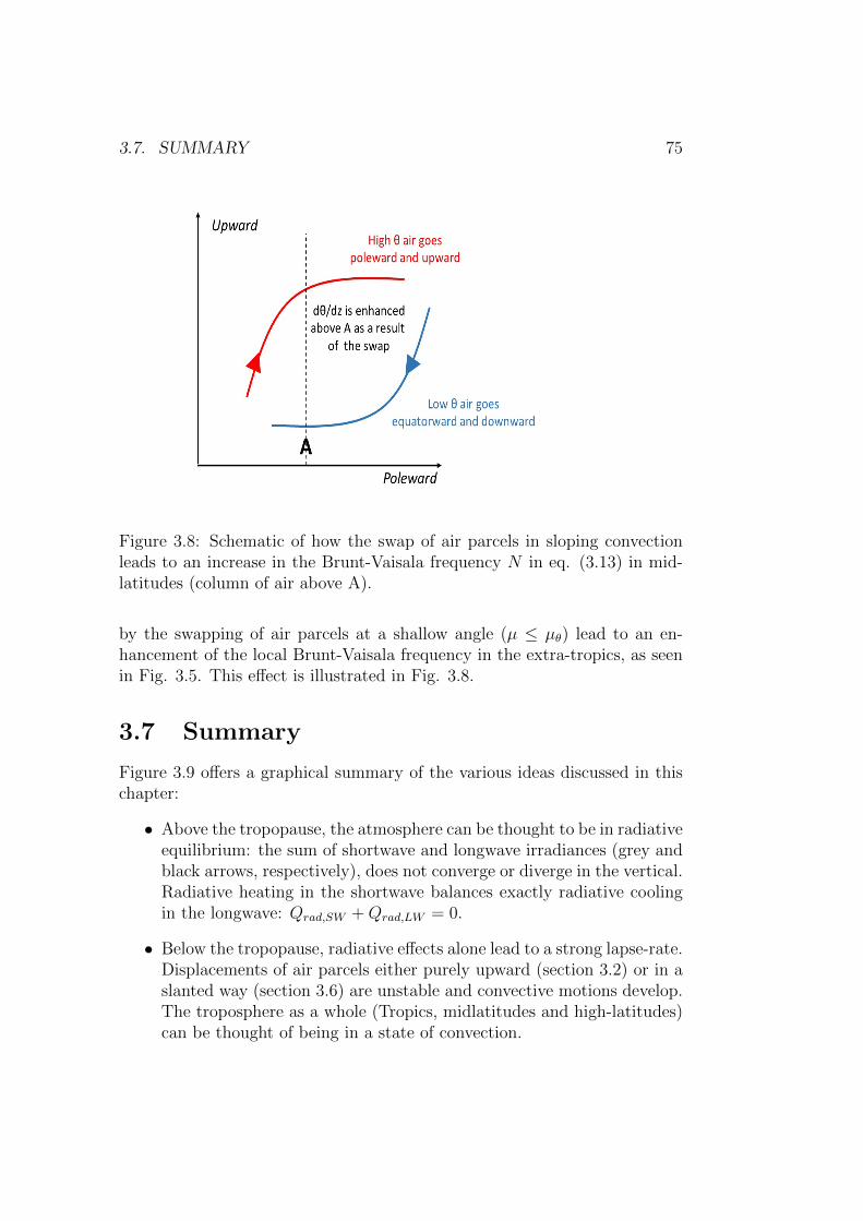
3.7. SUMMARY 75
Figure 3.8: Schematic of how the swap of air parcels in sloping convectionleads to an increase in the Brunt-Vaisala frequency N in eq. (3.13) in mid-latitudes (column of air above A).
by the swapping of air parcels at a shallow angle (µ ≤ µθ) lead to an en-hancement of the local Brunt-Vaisala frequency in the extra-tropics, as seenin Fig. 3.5. This effect is illustrated in Fig. 3.8.
3.7 Summary
Figure 3.9 offers a graphical summary of the various ideas discussed in thischapter:
• Above the tropopause, the atmosphere can be thought to be in radiativeequilibrium: the sum of shortwave and longwave irradiances (grey andblack arrows, respectively), does not converge or diverge in the vertical.Radiative heating in the shortwave balances exactly radiative coolingin the longwave: Qrad,SW +Qrad,LW = 0.
• Below the tropopause, radiative effects alone lead to a strong lapse-rate.Displacements of air parcels either purely upward (section 3.2) or in aslanted way (section 3.6) are unstable and convective motions develop.The troposphere as a whole (Tropics, midlatitudes and high-latitudes)can be thought of being in a state of convection.

76 CHAPTER 3. RADIATIVE-CONVECTIVE EQUILIBRIUM
• Convection carries heat upwards (blue arrows, converging upward ata rate Qconv from the surface to the tropopause). This transfer coolsthe surface and heat the upper levels, leading to a weaker (but stillpositive) lapse-rate.
• Convective heating is opposed by a net radiative cooling, seen in thevertical divergence of the net longwave irradiances (black arrows): Qrad,SW+Qrad,LW +Qconv = 0.
3.8 Problems
Q1. In this question we treat the Earth’s atmosphere as dry and in hydro-static equilibrium.
(i) Show that the adiabatic lapse rate is simply Γ = Γd = g/cp,d wherecp,d = 1005Jkg−1K−1 is the specific heat capacity of dry air at constantpressure and g = 9.81ms−2 is gravity. Compute its numerical value inK/km.
(ii) Show that the actual lapse rate is Γ = Γd − Tθ∂θ∂z
.
(iii) In light of the result in (ii) discuss whether a dry atmosphere can havea lapse rate greater (or lower) than Γd.
Q2. Air flows over the ocean (so it is well-supplied with moisture), acrossthe coast, over a mountain which is 4 km high and down to a plateau onthe far side at 1 km above sea level. Estimate the difference in temperaturebetween sea level on the windward side and at the surface of the plateau.[Take Γd = 10K/km and Γm = 6.5K/km].
Q3. Relative humidity (RH) is defined as the ratio of the vapour pressurefound in a sample of air at temperature T to that found when vapour andliquid water are in thermodynamic equilibrium at the same temperature:RH = e/eeq(T ). Discuss whether the situations below correspond to a stateof thermodynamic equilibrium: (i) Room temperature, RH = 0.7 (ii) pre-cipitation falling into a dry air mass, RH = 0.5 (as can happen on the edgeof a cloud).
Q4. We study a simple model of radiative equilibrium (Fig. 3.10) by treatingthe atmosphere as a two-layer system. Each of these layers is assumed to
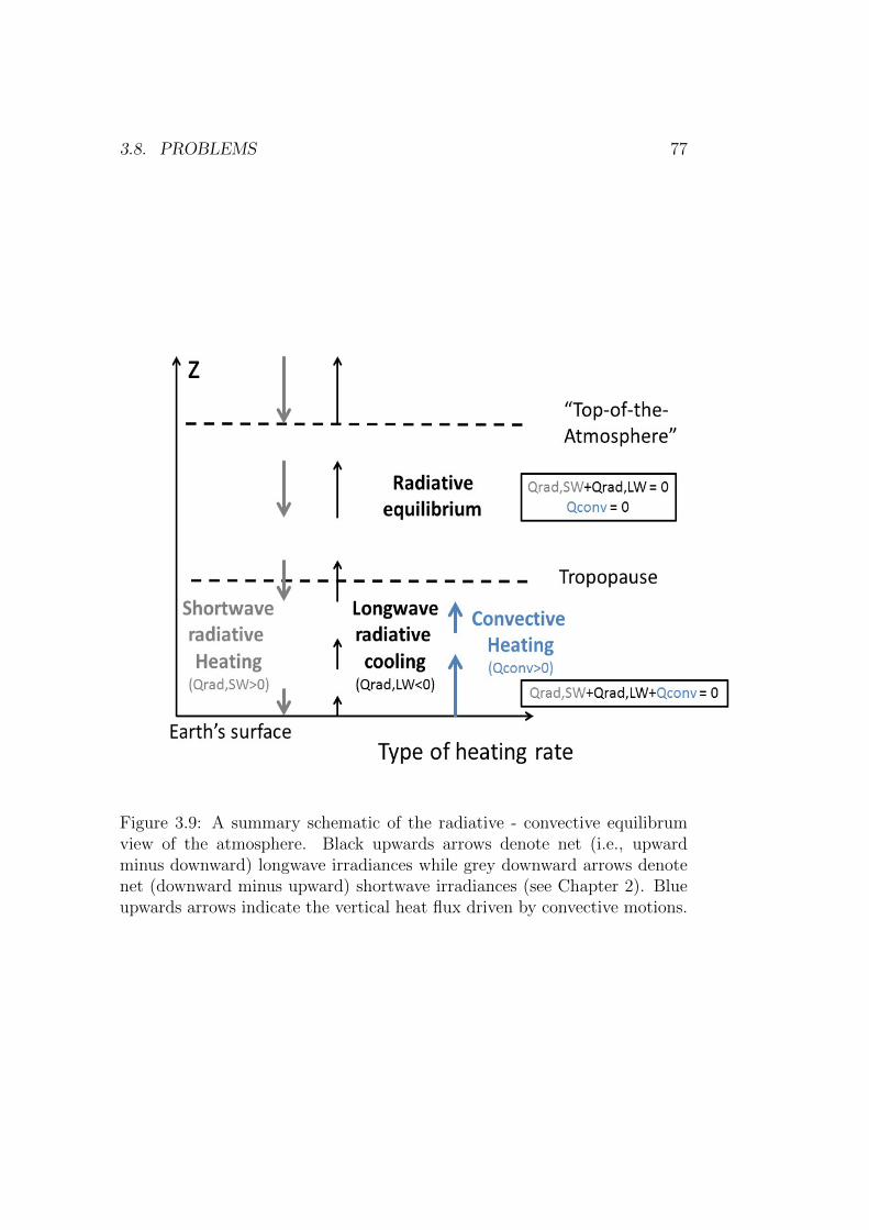
3.8. PROBLEMS 77
Figure 3.9: A summary schematic of the radiative - convective equilibrumview of the atmosphere. Black upwards arrows denote net (i.e., upwardminus downward) longwave irradiances while grey downward arrows denotenet (downward minus upward) shortwave irradiances (see Chapter 2). Blueupwards arrows indicate the vertical heat flux driven by convective motions.

78 CHAPTER 3. RADIATIVE-CONVECTIVE EQUILIBRIUM
Figure 3.10: Simple radiative equilibrium model. The surface receives solarradiation (σT 4
e ≡ So(1 − αP )/4) and emits infrared radiation upward. Theatmosphere consists of two layers of longwave emissivity unity and shortwaveabsorptivity zero.
radiate like a blackbody in the infrared. The Earth’s surface is also treatedlike a blackbody. The atmosphere is assumed to be completely transparent tosolar radiation, so that at each level, the solar flux is So(1−αP )/4. Computethe radiative equilibrium temperatures Ts (surface), T1 (lower atmosphere)and T2 (upper atmosphere).
Q5. The temperature profile predicted in the previous question is not stableto vertical displacements of air parcels. The latter lead to convective motionsand a new temperature distribution close to an adiabat. To represent thissimply, we fix the temperature difference ∆T = T1 − T2 = Ts − T1 in theprevious model, and also acknowledge the presence of additional heatingterms: a surface heat exchange Fs and a convective heat flux Fc (Fig. 3.11).
(i) Taking the two atmospheric layers to be at a pressure of 700hPa and400hPa respectively, and using your answers in Q3, check that indeedthe radiative equilibrium temperature profile is unstable. You may takethe surface pressure to be 1000hPa.
(ii) Before doing any calculation, do you expect the surface temperatureto decrease or increase when the fluxes Fs and Fc are included in themodel?

3.8. PROBLEMS 79
Figure 3.11: Addition of convective fluxes, Fs and Fc to the simple radiativeequilibrium model.
(iii) Solve for the temperature Ts, T1 and T2 as a function of Te and ∆T .
(iv) Solve for the convective flux Fc and the surface heat exchange Fs. Ex-press your answer as a function of Te and the non dimensional param-eter x = ∆T/Te.
(v) Find a plausible value for x and discuss the range of values of thisparameter for which the model makes sense. Also check that for thisrange of values the model agrees with your answer in (ii).
Q6. Using Figs. 1.5 and 3.2, estimate the kinetic energy gain in slopingconvection –eq. (3.31). How does this compare with your guess for thekinetic energy in storms?
Q7. A parcel of air has the same potential temperature than the environmentat t = 0 and z = 0, and an upward velocity wo = 10cm/s. Find its heightafter 1mn if (i) N2 = 10−4s−2 (ii) N2 = −10−4s−2. (iii) N2 = 0. Neglect theeffects of moisture on the motion.
Q8. The temperature structure in Fig. 1.3 in the mesosphere is very strange.In the Summer Hemisphere, the mesopause has T ≤ −100C while it is about70C warmer in the Winter Hemisphere!
80 CHAPTER 3. RADIATIVE-CONVECTIVE EQUILIBRIUM
(i) Estimate the mesospheric lapse rate (i.e., from stratopause to mesopause)in the summer and winter hemispheres
(ii) Sketch how θ(z) looks like in the summer and winter hemispheres
(iii) Show that the profiles you have plotted in (ii) are consistent with theBrewer-Dobson circulation sketched in the ppt slides for Chapter 1.
Chapter 4
Atmospheric motions
Key concepts: Eulerian and Lagrangian descriptions of motions, mate-rial derivative, Coriolis force, Rossby number, geostrophic balance, “thermalwind”, rotational and divergent flows, vorticity, Rossby waves.
The vertical instability associated with N2 < 0 in Chapter 3 is at theheart of convective cells and cloud clusters with horizontal scales rangingfrom a few km up to 100km. Updrafts and downdrafts in such systemsare however not the sole motions driven by radiative processes. Indeed, thenet radiative loss at high latitudes and the net radiative heat gain at theequator set up a whole range of motions. On scales of ≈ 1000km, we findthe traveling weather systems familiar at our latitudes, and their embeddedcold and warm fronts (≈ 100km). On even larger scale (10, 000km) we findplanetary cells organized in east - west (Walker cell) and north-south (Hadleycell) directions –see Fig. 4.1 for a summary. In this chapter we study thesemotions from first principles (Newton’s second law in a rotating frame ofreference). As we shall see, the Earth’s rotation has a profound impact onthe dynamics, giving a (counter-intuitive) rigid or solid - like behavior toatmospheric motions on large scales.
4.1 Equations of motions
These are simply the three components of the “momentum” equation (New-ton’s second law). Compared to the classical mechanics you have dealt withso far, the difficulties and novelty lie in:
(i) the “fluid nature” of the motion, air parcels transporting their ownmomentum (material derivative)
81

82 CHAPTER 4. ATMOSPHERIC MOTIONS
Figure 4.1: Space and time scales of atmospheric motions.
(ii) the Earth rotation, which introduces new forces as seen by an observerat a fixed location on the planet. The effects of rotation on motionsare huge as is most spectacularly illustrated with the “Taylor columns”(see Youtube video and the paper by Taylor (1923) on Blackboard).
(iii) the sphericity of the Earth, which introduces mathematical complexityand a “channel-like” geometry to the study of atmospheric motions.
4.1.1 Forces acting on a parcel of air
Per unit mass, these are simply: the acceleration due to gravity (kept toa constant g = 9.81ms−2 for practical purposes, owing to the thinness ofthe atmosphere compared to the Earth’s radius), the pressure gradient forcewe’ve seen in Chapter 3 (but now in 3D), and frictional (or viscous) forces,
a = g − α∇P + F fric (4.1)
Note that in this equation a is the acceleration vector in an inertial frame(say from an observer looking at the Earth from deep space), and α is thevolume per unit mass used extensively in Chapter 3.
4.1.2 Material derivative
Imagine a parcel of air undergoing an adiabatic ascent. Following the parcel,there is no change in its entropy. At a fixed location, however, an observer

4.1. EQUATIONS OF MOTIONS 83
might see a change in entropy since the parcel might originate from a warmerregion than that in which the observer is sitting. To make it clear that thechange “following the parcel” is a special case of derivative, we will write itas D/Dt. In the previous example, we would thus write,
Ds
Dt= 0 (4.2)
Mathematically, the change following the parcel (also called “Lagrangianderivative”) includes the parcel’s displacement. If we write that entropy isa function of space and time, i.e., s = s(x(t), y(t), z(t), t), a small change inentropy δs in a small time interval δt is, after Taylor expansion,
δs =
(∂s
∂t
)δt+
(∂s
∂x
)δx+
(∂s
∂y
)δy +
(∂s
∂z
)δz (4.3)
Dividing by δt and taking the limit, we thus identify D/Dt as,
Ds
Dt≡ lim
δt→0
δs
δt=∂s
∂t+ u
∂s
∂x+ v
∂s
∂y+ w
∂s
∂z(4.4)
Note that we have used the fact that the velocity components satisfy u =limδt→0 δx/δt, v = limδt→0 δy/δt and w = limδt→0 δz/δt.
The local change with time can then be mathematically identified with,
∂s
∂t=Ds
Dt− u.∇s (4.5)
in which we have introduced the velocity vector u = (u, v, w). This equationstates that the local change in entropy results from the change followingthe parcel minus that due to advection. The view encapsulated in (4.5) isreferred to as “Eulerian” (fixed location), as opposed to the “Lagrangian”(following a parcel) view in (4.2).
We used entropy in the previous example, but the concept applies toany variable, and even vector (applying the material derivative to each of itscomponent). For example, for the velocity vector,
u =Dr
Dt(4.6)
(You can readily check that this expression provides the identity u = u∂x/∂x =u, etc... since the coordinates x, y, z, t are independent).
Applying the notation to Newton’s second law, we obtain:
a = g − α∇P + F fric =Du
Dt= limδt→0
δu
δt(4.7)
84 CHAPTER 4. ATMOSPHERIC MOTIONS
This is the Navier-Stokes equation for fluid flow in an inertial frame of ref-erence. What is meant here is that the momentum of a fluid parcel changesalong its trajectory due to the gain / loss associated with gravitational, fric-tional and pressure forces. Note that the Du/Dt is a vector with components(Du/Dt,Dv/Dt,Dw/Dt). Each of those are non linear expressions, for ex-ample, for the third component of momentum,
Dw
Dt=∂w
∂t+ u
∂w
∂x+ v
∂w
∂y+ w
∂w
∂z(4.8)
showing that the upward motion carries its own upward momentum and thatthe latter is also carried by the horizontal flow.
4.1.3 Rotating frame of reference
The choice of the Earth as a frame of reference is natural. However, this isnot an inertial frame because it is accelerating (rotating) with respect to acoordinate system fixed in space. Newton’s law can be applied in the non-inertial frame if the acceleration of the coordinates is taken into account,introducing “apparent forces” in the equation of motion.
To introduce those, we need to relate the change of momentum of a parcelin the inertial frame1, denoted by (DuI/Dt)I to that measured in the rotatingframe of the Earth, denoted by (DuR/Dt)R. In this notation, uI and uR referto the velocity of a parcel in the inertial and rotating frames, respectively,while (D./Dt)I and (D./Dt)R denote the change following a parcel in theinertial and reference frames, respectively. Two important points need to beemphasized:
• we are talking about the same parcel of air here and we just describedifferently its momentum “history” (see Fig. 4.2) by measuring changesas (DuI/Dt)I or (DuR/Dt)R.
• such change in momentum history only arises because momentum is avector. In other words, in general(
DA
Dt
)I
6=(DA
Dt
)R
(4.9)
1We will consider that a coordinate system with the Earth’s centre as its origin (orbitingaround the Sun) provides such inertial frame. This is the idea introduced in Year 1 (Classi-cal mechanics) that a free falling object under the action of gravity behaves approximatelylike an inertial frame.

4.1. EQUATIONS OF MOTIONS 85
Figure 4.2: A simple apparatus (left) to illustrate how the trajectory ofan object appears different in an inertial and a rotating frame (right) ofreference. In the inertial frame, a small ball thrown at point O on a parabolicdish moves forward and backward (black trajectory on the right). Viewed inthe rotating frame of the dish, it describes a circle (blue trajectory). Frictionhas been ignored. Picture taken from Wallace and Hobbs’ textbook.
for any vector A (simply think about a constant vector in a rotatingframe: it will have a zero value of D/Dt in the rotating frame, but anon zero value in the inertial frame), but(
DB
Dt
)I
=
(DB
Dt
)R
(4.10)
is always true for any scalar B since we follow the same parcel (thinkabout measuring temperature of the parcel in Fig. 4.2: it does notmatter whether we describe its trajectory as a circle or a straight line,it is still the same temperature we measure since it is the same parcel).
We accept the result (proven in the Appendix) that, for any vector A,we have: (
DA
Dt
)I
=
(DA
Dt
)R
+ Ω×A (4.11)
in which Ω is the Earth’s rotation vector. Applying (4.11) to the vectorposition A = r (measured from the centre of the Earth), one recovers the

86 CHAPTER 4. ATMOSPHERIC MOTIONS
Galilean transformation of velocities between reference frames,
uI = uR + Ω× r (4.12)
Applying it to A = uI provides,(DuIDt
)I
=
(DuIDt
)R
+ Ω× uI (4.13)
which, after using (4.12), reads,(DuIDt
)I
=
(DuRDt
)R
+ 2Ω× uR + Ω× (Ω× r) (4.14)
(to obtain this result we acknowledge that (DΩ/Dt)R represents the changein the vector Ω at the location of the parcel, as seen in the rotating frame.At any given point along the trajectory, Ω is always the same since it is notaffected by the rotation effect encapsulated in (4.11). Thus (DΩ/Dt)R = 0.)
Rearranging, and using (4.7), we finally obtain,(DuRDt
)R
= g − α∇P + F fric − 2Ω× uR −Ω× (Ω× r) (4.15)
4.1.4 Coriolis and centrifugal forces
Comparing (4.15) with (4.7), one sees two new forces on the r.h.s, namelythe Coriolis and centrifugal forces. The latter only depends on the positionof the parcel (like a conservative force), and in effect acts to reduce gravity,
g′ ≡ g −Ω× (Ω× r) (4.16)
After noticing that −Ω × (Ω × r) = Ω2rH = ∇(Ω2r2H/2) where rH is thecomponent of r perpendicular to Ω, it is sometimes convenient to introducea slightly modified gravitational potential Φ such that,
g′ = −∇(Φgravi − Ω2r2H/2) ≡ −∇Φ (4.17)
We will in the following approximate surfaces of constant (net) gravitationalpotential Φ as spheres, with the net gravity given by g′.
The Coriolis force (−2Ω×uR) is required to explain why an object movingin a straight line in an inertial frame appears to have a curved path in arotating frame. (As will be apparent throughout this chapter, there is moreto it than this.) For now, let’s just analyze its effect on the momentumequation (4.15). Adopting the coordinate system in Fig. 4.3 (see also the

4.1. EQUATIONS OF MOTIONS 87
Figure 4.3: Local coordinate system (x, y, z). Longitude is denoted by λ,latitude by φ.
sidenote below), uR = (u, v, w) and Ω = Ω(0, cosφ, sinφ) in which φ islatitude and the three axes are i (West to East), j (South to North) and k(anti-parallel with g′). Thus the Coriolis force will have the components,
−2Ω× uR = −2Ω[(w cosφ− v sinφ)i+ u sinφj − u cosφk] (4.18)
Thus a parcel of air with a purely eastward velocity (u > 0, v = w = 0)will be accelerated southward in the Northern hemisphere (−u sinφ < 0)and northward in the Southern Hemisphere. The general rule is acceleratedto the right of the motion in the Northern Hemisphere, and to the left inthe Southern Hemisphere. You will also notice an upward acceleration, butthis is pretty small in comparison to gravity. We will proceed to a moresystematic analysis of the magnitude of each term in (4.15) in section 4.2.
Technical sidenote: local coordinate system. The (x, y, z) coordinate systemin Fig. 4.3 is local and cartesian. As such, it has some advantages comparedto that of spherical geometry. Specifically,
uR = ui+ vj + wk (4.19)
with u = r cosφDλDt, v = rDφ
Dt, w = Dr
Dt. Here r = R + z in which R is the
(mean) Earth’s radius, and since z R for practical purposes, one canfurther simplify and use,
u ≈ R cosφDλ
Dt, v ≈ R
Dφ
Dt, w =
Dz
Dt(4.20)

88 CHAPTER 4. ATMOSPHERIC MOTIONS
This system of coordinate however has the complication that the i, j,k vectorsvary with location, and as a result, (DuR/Dt)R 6= i(Du/Dt)R+j(Dv/Dt)R+k(Dw/Dt)R. Rather,(DuRDt
)R
= i
(Du
Dt
)R
+j
(Dv
Dt
)R
+k
(Dw
Dt
)R
+u
(Di
Dt
)R
+v
(Dj
Dt
)R
+w
(Dk
Dt
)R
(4.21)We will accept the result that,(
Di
Dt
)R
=u tanφ
Rj − u
Rk (4.22)(
Dj
Dt
)R
= −u tanφ
Ri− v
Rk (4.23)(
Dk
Dt
)R
=u
Ri+
v
Rj (4.24)
As a result,(DuRDt
)R
= [
(Du
Dt
)R
−uv tanφ
R+uw
R]i+[
(Dv
Dt
)R
+u2 tanφ
R+vw
R]j+[
(Dw
Dt
)R
−u2 + v2
R]k
(4.25)As can be easily checked the extra-terms purely reflect the spherical geometryof the Earth and disappear in the limit R→∞.
4.1.5 Mass conservation
Ignoring the loss of mass when it rains, and its gain when evaporation occursabove the Earth’s surface, the conservation of mass can be written as
∂ρ
∂t+ ∇.(ρuR) = 0 (4.26)
in which ρ = 1/α is the density of an air parcel. This equation is sometimescalled the “continuity equation”.
One interesting feature of this equation is that it is invariant to a changeof reference frame. Indeed, mass conservation in the inertial frame wouldread exactly the same with uR being replaced by uI (you can check thisby yourself readily after noticing that solid body rotation is a non divergentmotion). This is very unlike momentum conservation which, as we have justseen, requires a different formulation in the inertial and rotating frames. Thisis our first hint that momentum might not be the best variable to consider inrotating fluids. As we shall see later in this chapter, the curl of the velocityfield is much better suited (and its conservation equation is also invariantunder change of reference frame).

4.2. SCALE ANALYSIS OF THE EQUATION OF MOTIONS 89
4.2 Scale analysis of the equation of motions
The momentum equation (4.15) is quite complicated and we would not govery far if we were not able to simplify it further. To do so we are going touse a technique similar to dimensional analysis in which we are going to putorders of magnitude on each terms in (4.15). We will ignore the effects offriction and focus here on scales of motions typical of those seen on weathercharts, i.e. the sloping convection motions discussed at the end of Chapter3:
Lengthscale (horizontal) L ' 106m (a thousand kilometers)Lengthscale (vertical) H ' 104m (thickness of the troposphere)Velocity (u, v) U ' 10ms−1
Velocity (w) W ' 10−2ms−1
Time (t) T = L/U ' 105s (about one day)Horizontal Pressure gradient ∇LP ' 10hPa/1000km = 10−3Pam−1
Remember also that R = 6371km and 2Ω = 4π/1day ≈ 2× 10⁻⁴s−1.
NB: The scales for L,H,U, T and ∇LP are relatively intuitive (say from yourown estimate of windspeed looking at cloud displacement and a casual in-spection of weather charts). It is more difficult to estimate from observationswhat the scale for the vertical velocity W should be. One way to proceed isto use the continuity equation (4.26) and require that the horizontal and ver-tical derivatives contribute as much to the total divergence. You can easilycheck that this leads to W = HU/L ≈ 0.1ms−1. This estimate is an orderof magnitude larger than the one used above. The reason is that, we shallsoon see, weather systems are in geostrophic balance with very little verticalmotion (nearly non divergent motions).
4.2.1 Vertical momentum equation
The vertical component of (4.15) is, using (4.25),(Dw
Dt
)R
=u2 + v2
R+ 2Ωu cosφ− α∂P
∂z− g (4.27)
in which we have dropped g′ for g and have ignored the friction force.The first two terms on the r.h.s scale respectively as, U2/R and 2ΩU cosφ.Their strength relative to the acceleration of gravity are U2/gR ' 10−6 and2ΩU cosφ/g ≈ 2× 10⁻⁴ cosφ, respectively. The l.h.s has several components

90 CHAPTER 4. ATMOSPHERIC MOTIONS
since, (Dw
Dt
)R
=∂w
∂t+ u
∂w
∂x+ v
∂w
∂y+ w
∂w
∂z(4.28)
The first three have the same scale (since we have chosen T = L/U), namelyW/T , while the last term scales as W 2/H. The ratio of these to gravity isthus W/gT ≈ 10−8 and W 2/gH = 10−9, respectively. Note that because ofthe values listed above, U/L ≈ 10W/H so from now on we will simply scaleall D/Dt terms by simply dividing by T (i.e., (Dw/Dt)R ≈ W/T ).
The bottom line is that all the terms considered are negligible comparedto the acceleration of gravity and so, to a very good approximation, we cansafely use,
0 ≈ −α∂P∂z− g (4.29)
This is the “hydrostatic equation” introduced earlier in Chapter 3, expressinga near cancellation between the acceleration due to gravity and that due tothe vertical pressure gradient force.
To some extent the above scaling is misleading. It makes sense that grav-ity opposes the vertical pressure gradient, but the motions we are consideringconsist of pressure fluctuations superimposed on this state of pure hydro-static equilibrium. (In other words, the pressure fluctuations used above,i.e., 10hPa has nothing to do with the much larger pressure changes betweensurface and tropopause which is ≈ 750hPa). What we should really check iswhether this perturbed state satisfies the hydrostatic approximation. To dothis, write
α = α + α′ and P = P + P ′ (4.30)
where the bar denotes the background state in hydrostatic balance and theprime the fluctuations associated with weather systems. One can readilyobtain that,
α∂P
∂z+ g ≈ α
∂P ′
∂z− gα
′
α(4.31)
Putting orders of magnitude on each term, we find,
α∂P ′
∂z' (1kgm−3)
10hPa
10km= 10−1ms−2 (4.32)
and
−gα′
α≈ −gθ
′
θ' 9.81
3
300= 10−1ms−2 (4.33)
These terms are still much larger than all the others in (4.27) and so thehydrostatic approximation also applies to dynamic, as opposed to purely

4.2. SCALE ANALYSIS OF THE EQUATION OF MOTIONS 91
static situations,
0 ≈ α∂P ′
∂z− gα
′
α(4.34)
Most climate models use this approximation. (Among other things it allows achange of vertical coordinate z → P which simplifies considerably the modelnumerics).
NB?: You might rightly notice that the momentum balance (4.34) is differentthan the one used in Chapter 3 for sloping convection. What was missingthere is the fact that the parcels ascending and descending are embedded ina wave, with associated pressure variations. Their vertical gradients are theprimary mechanism opposing the buoyancy force, not vertical acceleration ofthe parcels. Returning to Fig. 3.7, as parcel A goes up, it gains kinetic energythrough the work of buoyancy force (and as we know from section 3.6 this ismaximized if it moves at an angle equal to half the slope of the θ surfaces).From eq. (4.34), we now know that it looses kinetic energy because of adversevertical pressure gradients. The later act as a brake on the wave whose energysource is the work computed in section (3.6).
4.2.2 Horizontal momentum equation
The two components of the horizontal momentum equations take the form,(Du
Dt
)R
= −uwR
+uv tanφ
R+ 2Ωv sinφ− 2Ωw cosφ− α∂P
∂x(4.35)(
Dv
Dt
)R
= −vwR− u2 tanφ
R− 2Ωu sinφ− α∂P
∂y(4.36)
Scaling these terms, we obtain (from left to right): U/T ≈ 10−4, UW/R ≈10−8, U2/R ≈ 10−5, ΩU sinφ ' 10−3 sinφ, ΩW cosφ ≈ 10−6 cosφ andα∇LP ' 10−3 (using the surface value for α ' 1m3/kg) for the zonalmomentum equation. Likewise, for the meridional momentum equation:U/T ≈ 10−4, UW/R ≈ 10−8, U2/R ≈ 10−5, ΩU sinφ ≈ 10−3 sinφ, andα∇LP ≈ 10−3.
Looking at these numbers it becomes clear that, as long as we are not tooclose to the equator where sinφ = 0, the approximate form of the horizontalmomentun equation is,
0 ' +2Ωv sinφ− α∂P∂x
(4.37)
0 ' −2Ωu sinφ− α∂P∂y
(4.38)

92 CHAPTER 4. ATMOSPHERIC MOTIONS
This approximation is called the geostrophic approximation, expressing anear cancellation between the acceleration due to the horizontal pressuregradient and Coriolis forces. One way to “visualize” this balance is that airparcels tend to flow along lines of constant pressure (anticlockwise around alow pressure system in the extra-tropics in the Northern Hemisphere).
After these two terms the next larger one is (Du/Dt)R for the zonalmomentum equation and (Dv/Dt)R for the meridional momentum equation.Both terms scale as U/T = U2/L. How small is this term compared to theCoriolis force is measured by a non dimensional number called the Rossbynumber (Ro),
Ro ≡U
2ΩL(4.39)
In other words, the smaller the Rossby number, the closer we are to geostrophicbalance. For the scales considered at the beginning of section 4.2, Ro ≈ 0.1.
NB: Not all atmospheric motions have small Rossby numbers. For example,hurricanes have typical windspeed U = 30ms−1 and horizontal lengthscaleL = 100km, yielding Ro ≈ 30/(2.10−4 × 105) = 1.5. Thus the geostrophicapproximation is not valid for hurricanes and advection of momentum by thehorizontal flow plays a key role in their dynamics.
4.2.3 The thermal wind relation
The smallness of the Rossby number is the main reason why the Earth rota-tion has so much influence on weather systems and many other motions. Wehave everything at hand to see straight away one of the powerful constraintsresulting from Ro 1, namely a constraint on how motions vary with height.
All we need are the approximate momentum equations (4.29), (4.37) and(4.38). Take the vertical derivative of (4.37), yielding,
f∂v
∂z≈ ∂
∂z[α∂P
∂x] (4.40)
in which we have introduced the Coriolis parameter,
f ≡ 2Ω sinφ (4.41)
Using (4.29), this can be rewritten as,
f∂v
∂z≈ ∂α
∂z
∂P
∂x− ∂α
∂x
∂P
∂z(4.42)
Likewise,
f∂u
∂z≈ −∂α
∂z
∂P
∂y+∂α
∂y
∂P
∂z(4.43)

4.2. SCALE ANALYSIS OF THE EQUATION OF MOTIONS 93
or, in vector form,
f∂V
∂z≈ (∇α×∇P )H (4.44)
in which V = ui + vj is the horizontal velocity vector and the subscript Hindicates we only consider the horizontal component.
The terms on the r.h.s of (4.44) vanish if α = α(P ). That is, in suchcondition, the horizontal velocity field cannot vary with height! –see thenote below on “Taylor columns”. More realistically, in the atmosphere α =α(T, P ) and the terms on the r.h.s do not vanish. Rather they set a constrainton how much the horizontal wind can vary with height.
A geometrical derivation brings more insight into these relations. Usingthe triple product rule for mixed derivative and the hydrostatic approxima-tion, one has,
α
(∂P
∂x
)z
= −α(∂z
∂x
)P
(∂P
∂z
)x
= g
(∂z
∂x
)P
(4.45)
which relates the pressure gradient to the slope of a pressure surface. As aresult, the difference in meridional wind (v) between two heights (z1 > z2)is, using the geostrophic balance,
v2 − v1 =g
f
(∂z
∂x
)P2
− g
f
(∂z
∂x
)P1
(4.46)
Likewise, for the zonal wind,
u2 − u1 =g
f
(∂z
∂y
)P1
− g
f
(∂z
∂y
)P2
(4.47)
These relations show that variations with height of the geostrophic windreflect horizontal gradients in the thickness between two pressure surfaces(Fig. 4.4). The thickness is itself directly related to temperature since thehydrostatic equation can be rewritten, using the ideal gas law (and neglectingmoisture), as,
∂ lnP
∂z= − g
RdT(4.48)
This indeed shows that for two given pressure surfaces (P1, P2), the thicknessbetween them (= z1 − z2) increases with the temperature of the layer of airsandwiched between these two surfaces,
z1 − z2 =
∫ z1
z2
dz =
∫ P2
P1
RdT
gd lnP (4.49)

94 CHAPTER 4. ATMOSPHERIC MOTIONS
Figure 4.4: The variations of the geostrophic wind with height reflect horizon-tal temperature variations: in the Northern Hemisphere (shown in picture),winds increasing with height have cold air to their left (if x is interpreted asthe east - west distance, the figure indicates southward wind v1 < 0 at upperlevel and northward wind v2 > 0 at low level). The distance between twopressure surfaces (the thickness) increases with temperature. In this diagramtwo pressure surfaces (P = P1 and P = P2) are shown in black, being at aheight z = z1(x) and z = z2(x), respectively.

4.3. THE VORTICITY VIEW 95
This is why the wind variations in (4.46)-(4.47) are called the “thermal wind”relations.
A vivid illustratioon of the thermal wind relation is also found in Fig.1.3 in Chapter 1. If we look for example at the winter hemisphere at 30,one observes that the contours of velocity close on themselves at a heightof about 10km (i.e., there is a wind maximum here, the Jet Stream). Thusbelow the maximum the wind increases with height but above the maximumthey decrease with height. The thermal wind relation shows that this mustbe associated with a reversal of the equator-to-pole temperature gradient.Indeed the Tropics are warmer than the Poles below 10km but are colder (!)above this level in the lower stratosphere.
NB?: The thermal wind relation offers insight into the “Taylor’s column”effect discussed at the beginning of this chapter. In a fluid of constant den-sity, it predicts ∂u/∂z = ∂v/∂z = 0. So the horizontal motion has to beindependent of height and we cannot expect the motion above the obstacle tobe solely limited to its vicinity. It happens that for small Rossby number andconstant density, one can also predict ∂w/∂z = 0 which implies that therecan be no motion above the obstacle at all (this would require having w nonzero just above the obstacle but zero away from it).
4.3 The vorticity view
4.3.1 The geostrophic flow, vorticity and divergence
The approximations derived in section 4.2 are very useful and allow to un-derstand the basic structure of atmospheric motions. However, you mighthave noticed that they do not include time derivatives. In other words, theyare just diagnostic relationships. Were you to forecast the weather based onthem, you would go nowhere!
The breakthrough to achieve this task came in the 1950s when it wasrealized that the geostrophic flow is rotational: it goes around pressure cen-ters (cyclones or anticyclones) but does not cross much the pressure lines.And so it became clear that what needs to be forecast is not momentum butvorticity ζ, the rotational (or curl) of the velocity field,
ζ ≡∇× uR (4.50)
To see the importance of vorticity, simply consider its vertical component
96 CHAPTER 4. ATMOSPHERIC MOTIONS
(ζ) in the local coordinate system,
ζ ≡ ζ.k =∂v
∂x− ∂u
∂y(4.51)
On the scales considered in section 4.2, one can, for practical purposes furthersimplify the geostrophic balance as,
v ≈ αofo
∂P
∂x, and u ≈ −αo
fo
∂P
∂y(4.52)
in which αo and fo are typical values of the specific volume and the Coriolisparameter over the region of interest. From this,
ζ ≈ αofo
(∂2P
∂x2+∂2P
∂y2
)(4.53)
while, the horizontal divergence of the (relative) flow δ is,
δ ≡ ∂u
∂x+∂v
∂y≈ 0 (4.54)
Thus indeed, the geostrophic flow is close to being purely rotational, i.e.,containing vorticity but no divergence. For such flows a streamfunction ψcan be introduced from the definition,
u ≡ −∂ψ∂y
and v =∂ψ
∂x(4.55)
Comparison of (4.52) with (4.55) shows that ψ ≈ αoP/fo: the horizontalflow follows approximately lines of constant pressure.
The concept of vorticity comes from Fluid Mechanics and is thus muchmore general than the special case of geostrophic flows. The video shown inthe lecture illustrates its presence or absence in simple flows (e.g., solid bodyrotation, source/sink flows in a kitchen sink –link provided on Blackboard).
Technical note: An important result is that a flow in solid body rotation hasa vorticity equal to twice the rate of rotation. A simple derivation can beobtained as follows. Consider a tank of water rotating around a vertical axisat a rate Ω. One can compute the vorticity of any fluid parcel embedded in thisflow by considering an anti-clockwise closed contour made of two lines r = r1and r = r2 (with r1 = r2 + δr, i.e., we are considering a very small contour)joined by two radial lines making a small angle δθ. From Stokes’ theorem,∮u.dl =
∫∫(∇×u).dS =
∫∫ζdS, which in polar cylindrical geometry, reads
u1r1δθ−u2r2δθ = ζδrδθ(r1+r2)/2. In solid body rotation u1 = Ωr1 and u2 =Ωr2, hence, Ω(r21−r22)δθ = ζδrδθ(r1+r2)/2. Since r21−r22 = (r1−r2)(r2+r1),one obtains ζ = 2Ω.
4.3. THE VORTICITY VIEW 97
4.3.2 Predicting the vorticity of the flow: the vorticityequation
We are going to restrict ourselves to horizontal flows on the sphere, i.e.,flows which have exactly zero vertical motion (w = 0). In so doing weare admittedly taking an extreme limit (for example all types of motionsdiscussed in Chapter 3 are excluded from this category), but it helps tosee more clearly how vorticity can be predicted. As it happens, horizontalmotions of planetary scales dominate the variability of atmospheric flows ontimescales greater than a week or so, so this is not an academic problembut rather, one of great importance for seasonal and climate prediction (seesection 4.3.3).
We thus consider the motion of an “air shell” sandwiched between theEarth and a concentric outer shell, and let us denote the (constant) distancebetween the two spheres, i.e., the height of the air column, by d (Fig. 4.5).We are going to follow in a Lagrangian sense an initial volume of air andwe will neglect any effect of compressibility. Thus we take α = cst = αo.As a result, the volume of this air sample remains constant. Since d is alsoconstant, this implies that the surface area S of the sample is constant duringits motion (it can deform and change shape but its total area has to remainthe same). Focusing on flow of sufficiently large scale and small velocityamplitude, the Rossby number is very small. The thermal wind relation thusapplies and without temperature variations (α = cst) this implies that thehorizontal velocity vector is constant with height. We can thus think of theflow as simply representing the horizontal motion of a rigid column of fluid(w = 0 by construction since the flow is bounded by two spherical shells–Fig. 4.5).
Let’s describe what happens to our column from the point of view of anobserver in an inertial frame (say viewed from Space). Its velocity is,
uI = uR + Ω× r (4.56)
We are going to use the result, known as Kelvin’s identity (proven in Ap-pendix), that if we follow a circuit made of fluid elements (hereafter called a“material contour”), i.e., any closed circuit within the column, we have,(
D
Dt
∮uI .ds
)I
≡∮ (
DuIDt
)I
.ds, (4.57)
in which ds denotes an infinitesimal segment of the circuit. Using the equa-tion of motion in an inertial frame (4.7), this can be rewritten as,(
D
Dt
∮uI .ds
)I
=
∮(−g − α∇P + F fric) .ds, (4.58)

98 CHAPTER 4. ATMOSPHERIC MOTIONS
Figure 4.5: Horizontal motion of a column of fluid (green shading, height d,horizontal surface area S) sandwiched between the Earth and a concentricouter shell.

4.3. THE VORTICITY VIEW 99
Since g = −∇Φgravi, we have∮g.ds =
∮dΦgravi = 0 (same starting and
end point in a closed contour). Likewise, because we take α to be constant,∮α∇P.ds = αo
∮dP = 0. If, in addition, we neglect friction, we come to
the conclusion that: (D
Dt
∮uI .ds
)I
= 0. (4.59)
From Stokes’theorem, this is also,(D
Dt
∫∫(∇× uI).dS
)I
= 0. (4.60)
where the integral is taken along any surface encircling the material contour.Using (4.56) and (4.50), this can be rewritten as,(
D
Dt
∫∫[ζ + ∇× (Ω× r)].dS
)I
= 0. (4.61)
Coming back to the motion in Fig. 4.5, a convenient choice of surface isclearly a sphere. With this choice, the normal dS is in the vertical direction(k in Fig. 4.5), and eq. (4.61) can be rewritten as,(
D
Dt
∫∫(ζ + f)dS
)I
= 0. (4.62)
Note that to arrive at this expression, we have used the result (shown in theAppendix) that ∇ × (Ω × r) = 2Ω. We now take the limit in which thehorizontal cross section of the column of air in Fig. 4.5 is infinitesimally small.Then S → dS is constant following the flow from the previous arguments,but we now also know, from (4.62), that the product of (ζ + f)S must beconstant following the flow. Hence we obtain the deceptively simple “vorticityequation”:
ζ + f = cst (following the flow) (4.63)
As we illustrate in the following section, this equation provides everythingwe need to predict the motion in Fig. 4.5.
Although we derived this equation by describing a material circuit in aninertial frame, the end result should be independent of that choice. Indeed,using the fact that (DB/Dt)I = (DB/Dt)R for any scalar B, we can as wellwrite, (
D
Dt
∫∫(ζ + f)dS
)R
= 0. (4.64)
One could derive this equation by following the same procedure as above inthe rotating frame of the Earth, but this would involve the (more mathemat-ically involved) calculation of a “torque” by the Coriolis force.
100 CHAPTER 4. ATMOSPHERIC MOTIONS
The variables ζ and f refer to the projection of the vorticity vectors ζ and2Ω onto the local vertical. There is a more general equation for the absolutevorticity vector ζa = 2Ω+ζ but we will not discuss it in this course (you cansee this equation in the picture on the “Welcome to Atmospheric Physics!”page at the beginning of these notes. If you’re interested I have included aderivation in the Appendix).
NB1?: In the inertial frame, the local rate of rotation of a fluid parcel is twicethe quantity ζ + f , which is called the “absolute vorticity” (≡ ζa). It is thesum of the vorticity ζ (the “relative vorticity”) due to the relative motion ofthe parcel with respect to the solid body rotation of the Earth, and that due tothe solid body rotation of the parcel around the Earth’s axis (f , the “planetaryvorticity”). As the experiment in the vorticity video showed (specifically, thepart showing the vorticity meter in a solid body rotation of a fluid in a tank),in a solid body rotation the fluid locally rotates at the same angular velocityas the tank. The associated vorticity is twice this rate (see technical note insection 4.3.1). In the rotating frame of reference, the local rate of rotationof a fluid parcel is just twice the relative vorticity (the vorticity meter in apure solid body rotation does not change for an observer rotating itself withthe tank).
NB2?: You could take the other limit in which the circuit in the above dis-cussion shrinks (like a the flow in a kitchen sink), i.e., S decreases. Theprediction from the circulation theorem is that (ζ + f)S must remain con-stant. Hence, ζ+f will have to increase. If the circuit shrinks over a limitedrange of latitude, this requires that the relative vorticity increases. In otherwords, a cyclone is intensifying. This is a decent model for the growth ofhurricanes. There are many other applications of the circulation theorem.An example is given in Q5 (Gulf Stream) of the problem sheet.
4.3.3 Rossby waves
A large class of motions of the atmosphere are loosely defined as being ofthe “planetary wave” type, to indicate that they are of sufficiently largespatial scale that they are affected by the fact that the Earth rotation vectorΩ has a projection on the local vertical which varies with latitude. Anexample is given in Fig. 4.6, showing the height of the 500hPa surface forthe Northern Hemisphere on 10 February 2014 –this approximately providesa streamfunction for the flow at mid-tropospheric levels from the discussionin section 4.3.1 and eq. (4.45). A wavenumber 2 structure is clearly apparentin the east-west direction, spreading from the North Pole to 30N .
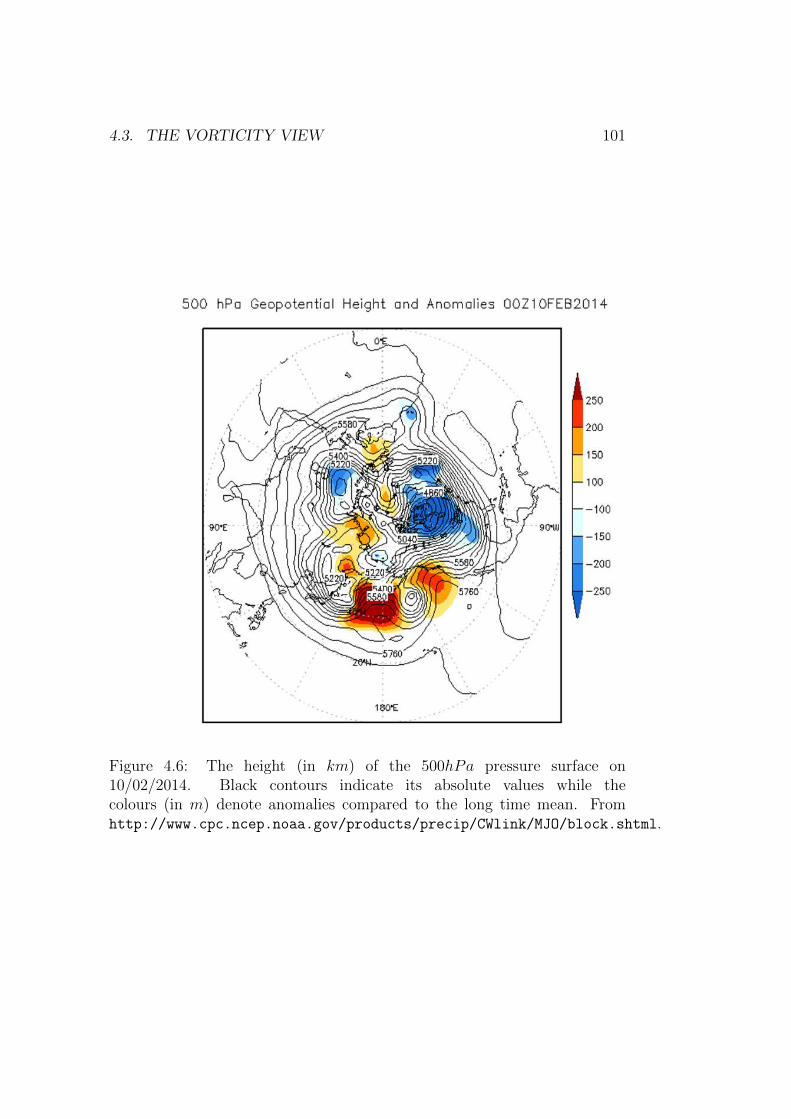
4.3. THE VORTICITY VIEW 101
Figure 4.6: The height (in km) of the 500hPa pressure surface on10/02/2014. Black contours indicate its absolute values while thecolours (in m) denote anomalies compared to the long time mean. Fromhttp://www.cpc.ncep.noaa.gov/products/precip/CWlink/MJO/block.shtml.

102 CHAPTER 4. ATMOSPHERIC MOTIONS
The Rossby number for these motions is particularly low Ro = U/2ΩL ≈10/(2 × 7.2 × 10−5 × 14, 000km) = 0.005 (using a wavenumber 2 at 45N)so that they satisfy the geostrophic balance and are nearly purely rotational(section 4.3.1). A lot of insight can be gained into these motions by using(4.64), which we express mathematically as:(
∂
∂t+ u
∂
∂x+ v
∂
∂y
)(f + ζ) = 0 (4.65)
Equation (4.65) states that absolute vorticity “sticks” to air parcels: youcan tell the origin of a given air mass from looking at its absolute vortic-ity (e.g., a low value of ζa typically originates from low latitudes)! A verypowerful tool.
The equation (4.65) supports linear waves called Rossby waves after theSwedish metorologist Carl Gustav Rossby who highlighted their dynamics inthe 1950s. Take the simplest possible case, i.e., linear motion on a state ofrest. Then (4.65) can be rewritten as,
∂ζ ′
∂t+ βv′ = 0 (4.66)
in which primes indicate perturbations and
β ≡ df
dy(4.67)
captures the latitudinal variation of the projection of Ω onto the local verti-cal. This equation can be solved by using the streamfunction ψ introducedin (4.55) and looking for plane wave solution2,
ψ′ ∝ ei(kx+ly−ωt) (4.68)
This provides the dispersion relation,
ω = − βk
k2 + l2(4.69)
and the associated phase velocity vP ,
vP = − β
k2 + l2(1, k/l) (4.70)
2The reason a streamfunction can be introduced rigorously here is that we are lookingat horizontal motion and have assumed constant density. Using these approximations, thecontinuity equation (4.26) predicts that the horizontal divergence of the flow has to bezero, i.e., ∂u/∂x+ ∂v/∂y = 0, hence u = −∂ψ/∂y and v = ∂ψ/∂x.

4.3. THE VORTICITY VIEW 103
The frequency of Rossby waves is typically much lower than that of theweather system we experience nearly daily (the latter were the subject ofsection 3.6 and, contrary to Rossby waves, the presence of upward and down-ward motion is crucial for their existence). For example, for the observationsin Fig. 4.6, I found ω ≈ 2π/43days−1 (using a wavenumber 2 at 45N for kand l = 2π/3000km). No wonder why these waves are studied tremendouslysince, owing to their long timescales, they introduce predictability to ourweather.
Rossby waves display a myriad of other interesting features:
• their phase speed is always westward (ω/k < 0). This follows directlyfrom the conservation of vorticity by fluid parcels, as encapsulated in(4.65) and illustrated in Fig. 4.7. The usual way to describe a wave interms of a restoring force is not useful for Rossby waves since, as em-phasized earlier, they are in geostrophic balance and the momentumequation does not say much about time evolution. This is why “vortic-ity thinking”, as illustrated in Fig. 4.7, brings much more insight intothe mechanism of propagation.
• they are associated with a transverse motion of air parcels. This isillustrated in Fig. 4.8, where the velocity vector (blue arrows) is alignedalong lines of constant pressure (by geostrophy) while the phase speed(black arrow) is at right angle. This is very different from other typesof waves supported by fluids (acoustic, gravity waves, i.e., swell) whichinvolve longitudinal motions. Again, this is a behaviour closer to thatof solids (e.g., shearwaves in the solid Earth generated by earthquakes).As you can see, this all has to do with β 6= 0.
• they carry east-west momentum across latitude circles. This propertyis illustrated in Fig. 4.8. Consider the portion of a latitude circlecorresponding to a zonal wavelength (marked by the red a-b-c line inthe figure). At a, a fluid parcel has u′ > 0 and v′ > 0, hence it carrieseastward momentum northward. At b, the parcel goes southward (v′ <0) but it has a negative eastward momentum (u′ < 0), hence again,it carries eastward momentum northward (removing negative eastwardmomentum from a region is like adding positive eastward momentumto it). At c, we have the repeat of what occurs at a. So averaged overa zonal wavelength, there is a net transport of eastward momentumnorthward. Mathematically this is expressed as a systematic positivecorrelation between u′ and v′: averaged over a zonal wavelength (east-west direction), the product u′v′ has a sign proportional to −kl (simplytake ψ′ ∝ sin(kx+ly−ωt) and check that u′v′ ∝ −klcos2(kx+ly−ωt)).

104 CHAPTER 4. ATMOSPHERIC MOTIONS
The bottom line is that Rossby waves carry zonal momentum withthem: this is the mechanism linking trade winds and westerlies thatwas mentioned in Chapter 1.
4.4 References
-Rossby and collaborators, 1939: Relation between variation in the intensityof the zonal circulation of the atmosphere and the displacement of the semi-permanent centers of action, J. Mar. Res., 38-55.
-Taylor, G. I., 1923: Experiments on the motion of solid bodies in rotatingfluids, J. Fluid Mech., 104, 213-218.
4.5 Problems
Q1. A thunderstorm moving in a sheared flow has the following scales: L =10km, H = 10km, U = 10ms−1, W = 1ms−1, f = 10−4s−1, P ′ = 10hPa.Determine whether the geostrophic and hydrostatic approximations apply tothis system.
Q2. An aeroplane is due to fly eastward over the ocean at 45N. At somemoment it is at an altitude of 6000m and a pressure altimeter indicates apressure of 100hPa. The pilot maintains this pressure altitude but noticesthat after 1 hour the radar altimeter indicates an absolute altitude of 5750m.How far, and in what direction, has the plane drifted off course? Clearlystate any assumptions you make. [Hint: this question is more difficult thanit looks.]
Q3. The derivation of the equation of motion (4.15), and its decompositioninto components (4.27), (4.35) and (4.36), was quite mathematical. Thisquestion aims at re-deriving those equations from a more intuitive perspec-tive.
(i) Particle moving purely east-west, i.e. u = (u, 0, 0) in the local frameof reference (i, j,k). By thinking about the particle’s circular motionaround the Earth at constant latitude φ, and its associated centrifu-gal force, show that it must experience an acceleration (Ω2R cosφ +u2/R cosφ + 2Ωu)(cosφk − sinφj). Identify the corresponding termsin (4.27) and (4.36).

4.5. PROBLEMS 105
Figure 4.7: Schematic of the propagation mechanism for Rossby waves inthe Northern Hemisphere (x−axis from west to east, y−axis from south tonorth). The horizontal line indicates lines of constant planetary vorticity(f), increasing towards the +y direction (f1 < f2 < f3). In presence of ananticyclone, these lines are bend and, for the case shown in the figure, lowlatitudes air parcels move northward to the west of the anticyclone, and highlatitudes air parcels move equatorward to the east (black arrows). Assumingthat these parcels did not possess significant relative motion before they weredisturbed by the anticyclone (i.e., their initial absolute vorticity is simply f),the conservation of their absolute vorticity ζ+f as they move requires that aregion of ζ < 0 develops to the west of the anticyclone (blue patch), and thata region of ζ > 0 develops to the east of the anticyclone (red patch). As aresult the anticyclone appears to move westward (an anticyclone correspondsto a region of ζ < 0), and creates a cyclone in its lee (a cyclone correspondsto ζ > 0). You can easily see from there why a wave of anticylone/cycloneswould naturally propagate westward.
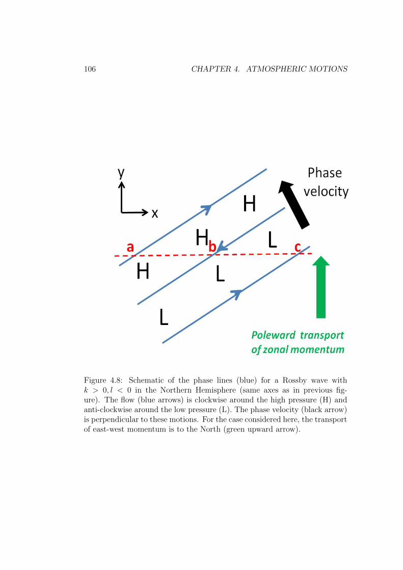
106 CHAPTER 4. ATMOSPHERIC MOTIONS
Figure 4.8: Schematic of the phase lines (blue) for a Rossby wave withk > 0, l < 0 in the Northern Hemisphere (same axes as in previous fig-ure). The flow (blue arrows) is clockwise around the high pressure (H) andanti-clockwise around the low pressure (L). The phase velocity (black arrow)is perpendicular to these motions. For the case considered here, the transportof east-west momentum is to the North (green upward arrow).
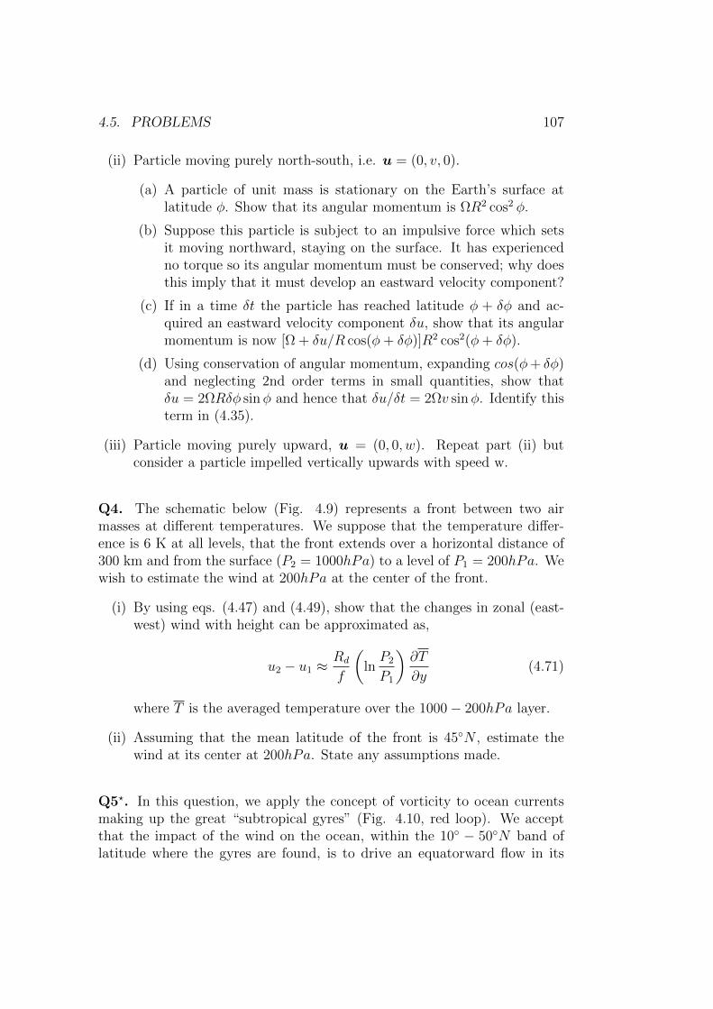
4.5. PROBLEMS 107
(ii) Particle moving purely north-south, i.e. u = (0, v, 0).
(a) A particle of unit mass is stationary on the Earth’s surface atlatitude φ. Show that its angular momentum is ΩR2 cos2 φ.
(b) Suppose this particle is subject to an impulsive force which setsit moving northward, staying on the surface. It has experiencedno torque so its angular momentum must be conserved; why doesthis imply that it must develop an eastward velocity component?
(c) If in a time δt the particle has reached latitude φ + δφ and ac-quired an eastward velocity component δu, show that its angularmomentum is now [Ω + δu/R cos(φ+ δφ)]R2 cos2(φ+ δφ).
(d) Using conservation of angular momentum, expanding cos(φ+ δφ)and neglecting 2nd order terms in small quantities, show thatδu = 2ΩRδφ sinφ and hence that δu/δt = 2Ωv sinφ. Identify thisterm in (4.35).
(iii) Particle moving purely upward, u = (0, 0, w). Repeat part (ii) butconsider a particle impelled vertically upwards with speed w.
Q4. The schematic below (Fig. 4.9) represents a front between two airmasses at different temperatures. We suppose that the temperature differ-ence is 6 K at all levels, that the front extends over a horizontal distance of300 km and from the surface (P2 = 1000hPa) to a level of P1 = 200hPa. Wewish to estimate the wind at 200hPa at the center of the front.
(i) By using eqs. (4.47) and (4.49), show that the changes in zonal (east-west) wind with height can be approximated as,
u2 − u1 ≈Rd
f
(lnP2
P1
)∂T
∂y(4.71)
where T is the averaged temperature over the 1000− 200hPa layer.
(ii) Assuming that the mean latitude of the front is 45N , estimate thewind at its center at 200hPa. State any assumptions made.
Q5?. In this question, we apply the concept of vorticity to ocean currentsmaking up the great “subtropical gyres” (Fig. 4.10, red loop). We acceptthat the impact of the wind on the ocean, within the 10 − 50N band oflatitude where the gyres are found, is to drive an equatorward flow in its

108 CHAPTER 4. ATMOSPHERIC MOTIONS
Figure 4.9: Schematics of temperature variations at a front.
upper (0− 1000m) layers. As water parcels flow equatorward, their absolutevorticity ζ + f is accordingly changed. Note that throughout this questionabsolute vorticity is not conserved, either because of the effect of the winds,or because of the effect of frictional forces near the continental shelves.
(i) Show that since the equatorward current is on the order of a few cm/sand its horizontal scale is that of the North Atlantic basin, the absolutevorticity of water parcel in the equatorward flow is approximately f .Determine the resulting loss of absolute vorticity along the equatorwardflow.
(ii) To close the mass budget, a “return” current must occur in the pole-ward direction. In the North Atlantic, this current is called the GulfStream. Considering that the latter has a magnitude of a few m/s andan horizontal extent of a few tens of km, do you think the approxima-tion ζa ≈ f is still valid in the Gulf Stream?
(iii) Based on your answer to the previous question, and thinking of the be-haviour of absolute vorticity within a closed loop around the subtropi-cal gyre, determine whether water parcels must gain or loose absolutevorticity in the Gulf Stream.
(iv) By thinking about the effect of horizontal friction on vorticity explainwhy the Gulf Stream is found on the east coast of the US and not onthe west coast of Portugal.
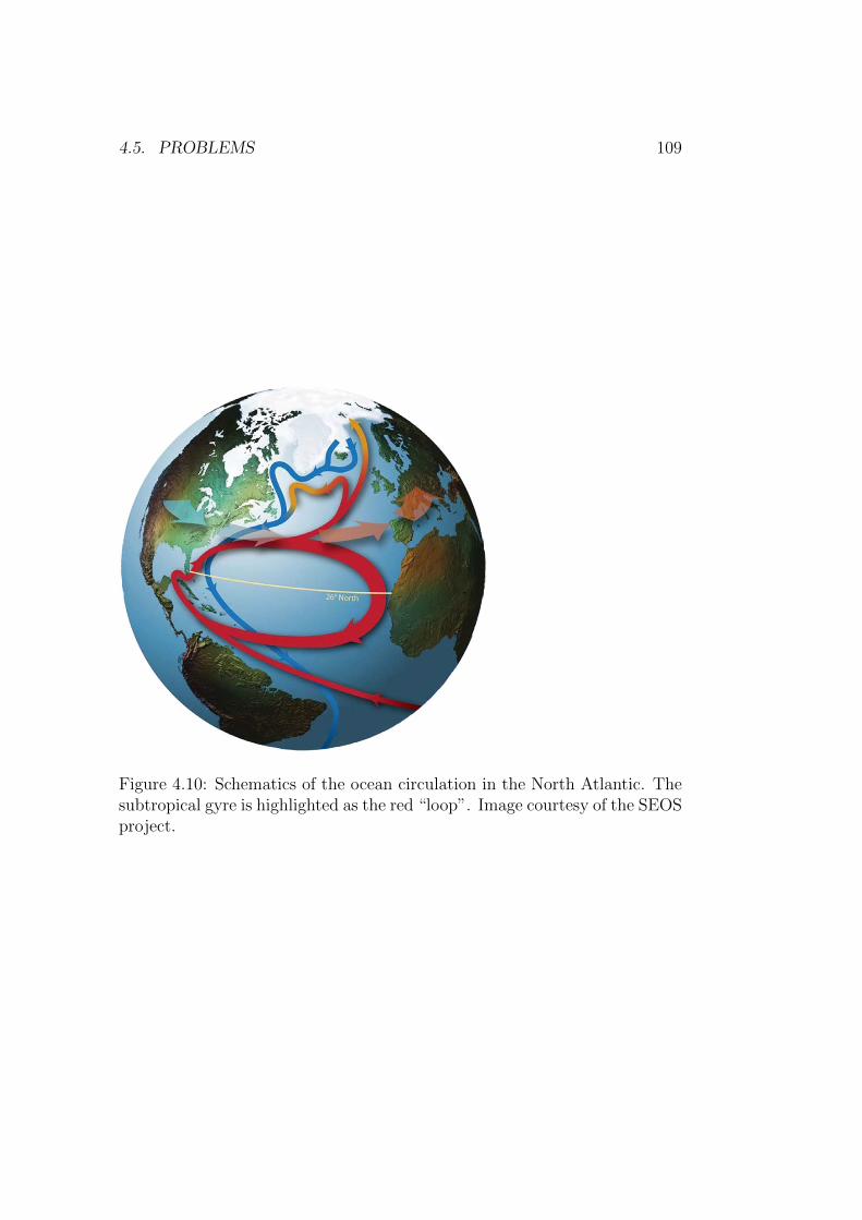
4.5. PROBLEMS 109
Figure 4.10: Schematics of the ocean circulation in the North Atlantic. Thesubtropical gyre is highlighted as the red “loop”. Image courtesy of the SEOSproject.
110 CHAPTER 4. ATMOSPHERIC MOTIONS
Q6. One sometimes reads or hears that, by analogy with atmospheric lowpressure systems, the flow in a bath tube which is being emptied circulates inopposite direction in the Northern and Southern Hemisphere. Give at leasttwo reasons why this is bonkers.
Q7. Past Exam Question (2003 no.4).
(i) What is vorticity and why is it useful for understanding the weather?
(ii) Consider a long-wave pattern at the level of non-divergence in a zonalcurrent of uniform constant velocity, U . From the principle of conser-vation of absolute vorticity and making the assumption that the totalvelocities are independent of latitude show the Rossby wave equationcan be written as:
(U − c)∂2v′
∂x2+ βv′ = 0 (4.72)
where c is the wave velocity, v′ the meridional velocity perturbationand β the meridional rate of change of the Coriolis parameter. Find anexpression for c in terms of the wavelength and β.
(iii) Calculate the wavelength of the Rossby wave if it appears stationary at50N when the zonal wind is 50ms−1. For the same zonal wind, whatwould happen to a wave of the same wavelength at lower latitudes?(The radius of the Earth is 6371 km).

Chapter 5
Climate change
We defined climate in Chapter 1 as the state of the atmosphere averaged overa sufficiently long time. What that time averaging period needs to be is notclear for several reasons. First, the atmosphere on its own is capable of fluc-tuations of its statistics over timescales of decades. The MIT meteorologistEd Lorenz (the one who is now associated with the “Butterfly effect”) talkedabout the atmosphere being an “almost intransitive system”, i.e., a systemwhose statistics can vary significantly over time (Lorenz, 1968). Second, theatmosphere interacts with other systems and this also leads to changes on avery wide range of timescales:
• seasonal to interannual, due to changes in sea surface temperature
• multidecadal to multi-centennial due to changes in the state of theoceans (temperature and circulation).
• centennial to millenial due to changes in the state of the ice sheets
• millions of years due to the motion of continental plates (tectonics)
In addition, the natural variability of solar activity, as well as the geometryof the Earth’s orbit around the Sun, and of its own axis of rotation, alsointroduces changes in the amount of solar energy reaching the top-of-the-atmosphere. These occur on timescales on the order of decades for the so-called “11-yr” solar cycle, and several tens of thousands of years to severalhundred of thousand years for the Milankovitch cycles (see the fascinatingaccount of their history in Imbrie and Imbrie, 1979).
We focus in this chapter on a very special type of climate change: theone caused by perturbations of the composition of the atmosphere as a resultof human activities, with a particular emphasis on the burning of fossil fuel(increase in carbon dioxide concentration). Only the physical aspects are
111

112 CHAPTER 5. CLIMATE CHANGE
discussed, with a focus on the ocean-atmosphere system. For a more holisticview of the problem, I highly recommend the short book by Prof D. Archer(2009).
5.1 Anthropogenic radiative forcing
As discussed in Chapter 2, carbon dioxide is a greenhouse gas owing to itstri-atomic structure. The major absorption band of the CO2 molecule iscentered near 15µm, which happens to be in the spectral region where theatmosphere emits most intensely infrared radiation (Fig. 1.6). Thus it isno surprise that the accumulation of carbon dioxide in the atmosphere isperturbing the heat balance of the Earth.
Figure 5.1 quantifies the magnitude of the change in downward radiationat the tropopause with respect to pre-industrial times. Carbon dioxide isseen to dominate the anthropogenic forcing, with an anomalous downwardenergy flux (infrared) on the order of 1.5Wm−2. Methane comes second witha forcing on the order of 1Wm−2 (as you can see in the plot this numberinvolves not only the direct effect of methane on radiation but its knock-oneffect on other greenhouse gases through chemical reactions). Note that someof the anthropogenic forcings act to cool the planet, for exemple aerosols,because they increase the reflection of solar radiation. This effect is bothdirect (aerosols reflecting directly the sunlight back to space) and indirect(by promoting the formation of clouds with smaller water drops and higheralbedo). Aerosols also have a warming effect by absorbing and re-emittinginfrared radiation which cancel partly the previous two. The net is estimatedto be a cooling on the order of ≈ 0.25 + 0.55 = 0.8Wm−2 in Fig. 5.1.
5.2 Response of the atmosphere to a sudden
doubling of CO2
We focus here on the CO2 impact only (infrared), and consider the “thoughtexperiment” of what would happen to the atmosphere if we were to suddenlymultiply its CO2 concentration by a factor of two. Even when restrictingattention to the atmosphere-ocean system only, as we’ll do, there are severaltimescales involved in this process:
• The first (fast, on the order of a few days to weeks) is that in which thetemperature field simply reflects the local change in radiative heatinginduced by doubling CO2 concentrations (i.e., increases where there is

5.2. RESPONSE OF THE ATMOSPHERE TOA SUDDENDOUBLINGOF CO2113
Figure 5.1: Anomalous (i.e., 2011 vs 1750) downward radiative flux at thetropopause in Wm−2. The radiative forcing of various constituents is listed.Figure taken from the 5th assessment report of the IPCC.
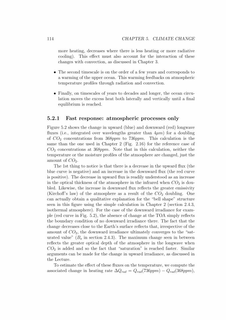
114 CHAPTER 5. CLIMATE CHANGE
more heating, decreases where there is less heating or more radiativecooling). This effect must also account for the interaction of thesechanges with convection, as discussed in Chapter 3.
• The second timescale is on the order of a few years and corresponds toa warming of the upper ocean. This warming feedbacks on atmospherictemperature profiles through radiation and convection.
• Finally, on timescales of years to decades and longer, the ocean circu-lation moves the excess heat both laterally and vertically until a finalequilibrium is reached.
5.2.1 Fast response: atmospheric processes only
Figure 5.2 shows the change in upward (blue) and downward (red) longwavefluxes (i.e., integrated over wavelengths greater than 4µm) for a doublingof CO2 concentrations from 368ppm to 736ppm. This calculation is thesame than the one used in Chapter 2 (Fig. 2.16) for the reference case ofCO2 concentrations at 368ppm. Note that in this calculation, neither thetemperature or the moisture profiles of the atmosphere are changed, just theamount of CO2.
The 1st thing to notice is that there is a decrease in the upward flux (theblue curve is negative) and an increase in the downward flux (the red curveis positive). The decrease in upward flux is readily understood as an increasein the optical thickness of the atmosphere in the infrared when CO2 is dou-bled. Likewise, the increase in downward flux reflects the greater emissivity(Kirchoff’s law) of the atmosphere as a result of the CO2 doubling. Onecan actually obtain a qualitative explanation for the “bell shape” structureseen in this figure using the simple calculation in Chapter 2 (section 2.4.3,isothermal atmosphere). For the case of the downward irradiance for exam-ple (red curve in Fig. 5.2), the absence of change at the TOA simply reflectsthe boundary condition of no downward irradiance there. The fact that thechange decreases close to the Earth’s surface reflects that, irrespective of theamount of CO2, the downward irradiance ultimately converges to the “sat-urated value” (Bo in section 2.4.3). The maximum change seen in betweenreflects the greater optical depth of the atmosphere in the longwave whenCO2 is added and so the fact that “saturation” is reached faster. Similararguments can be made for the change in upward irradiance, as discussed inthe Lecture.
To estimate the effect of these fluxes on the temperature, we compute theassociated change in heating rate ∆Qrad = Qrad(736ppm) − Qrad(368ppm),

5.2. RESPONSE OF THE ATMOSPHERE TOA SUDDENDOUBLINGOF CO2115
Figure 5.2: Changes in upward (blue) and downward (red) infrared fluxes(in Wm−2) as a result of a doubling of atmospheric concentrations of carbondioxide. The changes are shown as a function of pressure.

116 CHAPTER 5. CLIMATE CHANGE
with
∆Qrad =d
dz(∆F ↓ −∆F ↑) (5.1)
using the definitions and notations in Chapter 2. The calculation in Fig. 5.2was carried out in pressure coordinates rather than height z, so we must firstre-express the previous equation in pressure coordinates. To do so we usethe hydrostatic equation, yielding,
∆Qrad = −ρg d
dP(∆F ↓ −∆F ↑) (5.2)
The unit of Qrad is Wm−3 which is not particularly helpful. It is moreintuitive to convert this heating rate in units of K/day and this can be doneby simply dividing by ρcp. (Note that cp and not cv is used because we focuson an infinitesimal layer between P and P + dP , i.e., a layer of constantpressure). The result is shown in Fig. 5.3. One observes anomalous heatingof the troposphere, on the order of 0.1K/day and a larger cooling of theupper stratosphere and mesosphere (this increase in the magnitude mostlyreflects the little amount of mass at these high altitudes).
One can qualitatively understand these contrasting responses. The tropo-spheric warming results both from more absorption of the radiation emittedby the ground (same T but greater optical depth), and more infrared radia-tion emitted by the stratosphere. The stratospheric cooling is perhaps moresurprising but can be understood in the following way. First, the stratosphereemits more infrared both downward and upward, which tends to cool it. Inaddition, it also receives less upward infrared radiation from the troposphere,which also cools it. This effect is partly opposed by the increased opacity ofthe stratosphere with more CO2, i.e., more absorption of infrared radiationin the stratosphere, but the net is overwhelmingly a cooling.
The size of the anomalous heating is such that it would take about 10daysto reach a typical change of 1K in the troposphere. In a globally averagedsense, the atmosphere sees mostly ocean as its lower boundary. Because ofthe latter’s large thermal inertia, the surface temperature would change bymuch less in 10days. Thus the troposhere warms up but its lower layersremain “climatological”. The atmospheric lapse-rate then decreases whichmakes the atmosphere more stable to displacements of air parcels from lowlevels (Chapter 3) –note that the vertical structure in the anomalous heatingin Fig. 5.3 adds further to this “boundary effect”. This is reflected in weakerupdrafts/downdrafts and a general weakening of the atmospheric circulation.You’ll be pleased to learn that this effect was only emphasized recently inthe journal Nature Geosciences (Bony et al., 2013).
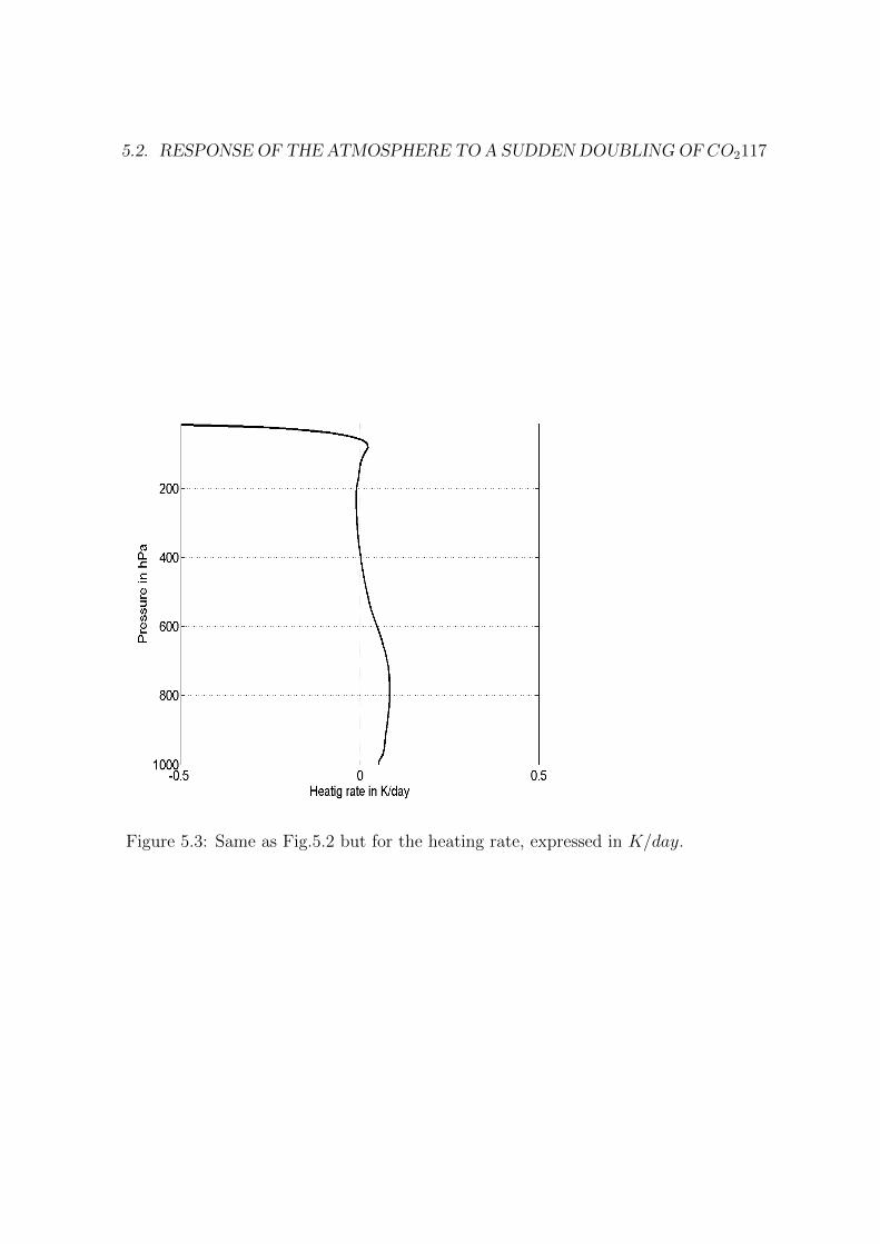
5.2. RESPONSE OF THE ATMOSPHERE TOA SUDDENDOUBLINGOF CO2117
Figure 5.3: Same as Fig.5.2 but for the heating rate, expressed in K/day.

118 CHAPTER 5. CLIMATE CHANGE
The same calculations can be carried out latitude by latitude, the re-sult being that the tropospheric heating is more pronounced at the equator(Fig. 5.4). This can be understood from Beer’s law, the reduction in upwardinfrared radiation at the tropopause being proportional to the amount ofradiation emitted by the air column, which is greater in the Tropics. Inter-estingly, this tropical enhancement is opposed by a larger downward radia-tive flux from the stratosphere at high latitudes (this simply reflects that thetropopause is lower down at the poles than at the equator, i.e., that there ismore “stratospheric mass” at the poles than at the equator). As can be seenin Fig. 5.4 though, the tropospheric effect dominates and the Tropics gainmore energy than the poles when doubling CO2 concentrations.
The tropical amplification of the heating mimics the situation in the timemean, whereby the Earth experiences an energy deficit at the poles and anenergy gain at the equator. Interestingly, this excess heating is truly realizedin the atmosphere (infrared heating), rather than mostly absorbed at the seasurface as is the case for the time mean (see Chapter 1). In other wordsthere is more available potential energy within the atmosphere to powerthe storms (Chapter 3). Assuming that conversion rates of this energy intokinetic energy of storms is unchanged, the sudden doubling of CO2 will leadto a change in the distribution of storms: either the same number but withhigher winds, or less weak storms, and / or more strong storms.
5.2.2 Slow response: the atmosphere interacts withthe upper ocean
Figure 5.2 indicates that there is a net anomalous downward radiative fluxat the Earth’s surface, with a magnitude ' 2Wm−2. The upper ocean iswell mixed over a layer of depth h ≈ 100m, and its heat capacity per unitarea is ρoco (density ρo = 1025kgm−3 and heat capacity of seawater co =4000Jkg−1K−1, respectively) so it would take a time ∆t to generate a changeof 1K, where
∆t = ρocoh1K
2Wm−2= 6.5years (5.3)
This rough estimate shows that the interaction with the ocean is importantin setting the response of the atmosphere to a CO2 change on timescalesbeyond a few years.
This upper ocean warming perturbs the radiative - convective equilibriumat fixed surface temperature response discussed in the previous subsection.A new type of equilibrium must be reached, in which a warmer ocean leadsto more destabilization of the atmosphere. An illustration of this effect is
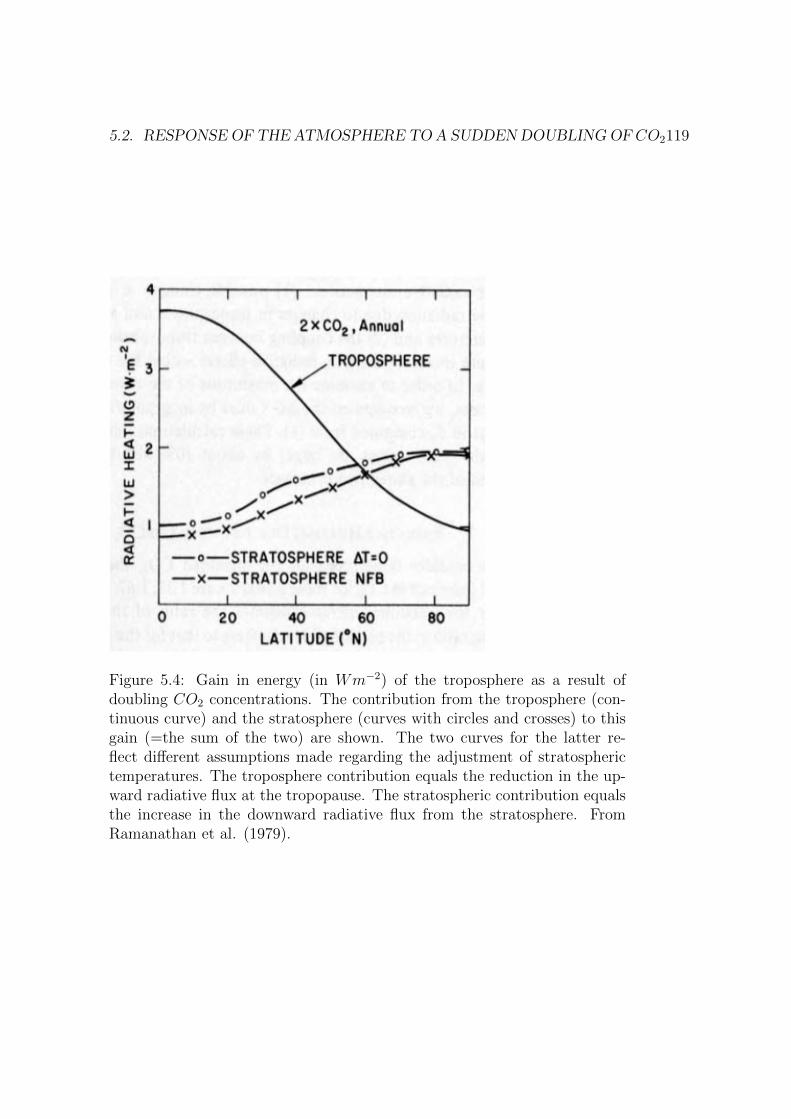
5.2. RESPONSE OF THE ATMOSPHERE TOA SUDDENDOUBLINGOF CO2119
Figure 5.4: Gain in energy (in Wm−2) of the troposphere as a result ofdoubling CO2 concentrations. The contribution from the troposphere (con-tinuous curve) and the stratosphere (curves with circles and crosses) to thisgain (=the sum of the two) are shown. The two curves for the latter re-flect different assumptions made regarding the adjustment of stratospherictemperatures. The troposphere contribution equals the reduction in the up-ward radiative flux at the tropopause. The stratospheric contribution equalsthe increase in the downward radiative flux from the stratosphere. FromRamanathan et al. (1979).
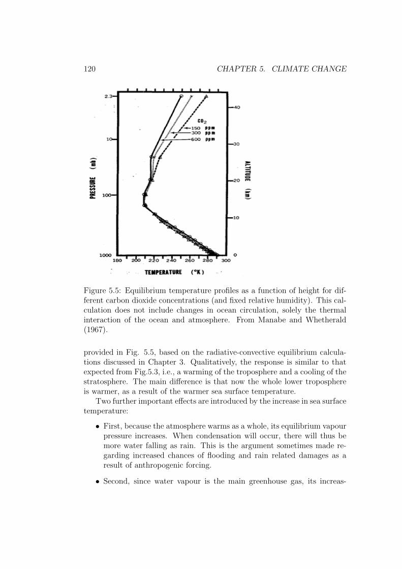
120 CHAPTER 5. CLIMATE CHANGE
Figure 5.5: Equilibrium temperature profiles as a function of height for dif-ferent carbon dioxide concentrations (and fixed relative humidity). This cal-culation does not include changes in ocean circulation, solely the thermalinteraction of the ocean and atmosphere. From Manabe and Whetherald(1967).
provided in Fig. 5.5, based on the radiative-convective equilibrium calcula-tions discussed in Chapter 3. Qualitatively, the response is similar to thatexpected from Fig.5.3, i.e., a warming of the troposphere and a cooling of thestratosphere. The main difference is that now the whole lower troposphereis warmer, as a result of the warmer sea surface temperature.
Two further important effects are introduced by the increase in sea surfacetemperature:
• First, because the atmosphere warms as a whole, its equilibrium vapourpressure increases. When condensation will occur, there will thus bemore water falling as rain. This is the argument sometimes made re-garding increased chances of flooding and rain related damages as aresult of anthropogenic forcing.
• Second, since water vapour is the main greenhouse gas, its increas-

5.2. RESPONSE OF THE ATMOSPHERE TOA SUDDENDOUBLINGOF CO2121
ing concentration in the atmosphere triggers a positive feedback loop:more water vapour leads to greater surface warming, which leads togreater surface evaporation and (assuming rainfall does not entirelycompensate), more water vapour in the atmosphere.
5.2.3 Very slow response: the atmosphere interactswith the ocean circulation
Both the changes in atmospheric heating rates and sea surface temperaturediscussed in the previous two subsections will lead to changes in atmosphericcirculation patterns (either shift or intensification, or both). These in turnwill alter ocean currents and the capacity of the ocean to transport heatlaterally and vertically. The associated timescales can be as fast as a decadeand as long as a millenium.
Figure 5.6 (right panel) illustrates the change in ocean heat contentthrough time in response to a sudden doubling of atmospheric CO2 in theEnvironmental Physics climate model (EPcm), a simple climate model codedin MATLAB (linked on Blackboard). One observes a rapid adjustment oftropical and high latitude upper ocean temperatures (red and blue curves),but it takes much longer to adjust the subsurface ocean temperatures (tropi-cal in magenta, high-latitudes in cyan). This longer adjustment correspondsto the time it takes to circulate waters through the different layers in themodel. If the ocean circulates water between upper and deeper layers withan intensity Ψ (in m3s−1) and if the deep layer volume is V , then it will takea time,
∆t = V/Ψ ≈ 1000m× (2.5× 1014m2)
10× 106m3s−1≈ 1, 000years (5.4)
to do so. To obtain this number, a thickness of 1000m was used for the deeplayer, a surface area equal to that of one hemisphere (EPcm covers only onesuch hemisphere) and a value of 107m3s−1 was used for Ψ (this is about tentimes the volume flux of all the rivers of the world).
The timescale in (5.4) is clearly reflected in the top-of-the-atmospherenet radiative flux (left panel) which, after a sudden increase to ' 4Wm−2
associated with the initial CO2 doubling, only very slowly goes back to zero(the new equilibrium)1.
1EPcm also displays the fast (weeks) and slow (years) response discussed in the previoussubsections. You can very easily convince yourself of this by running the model over onemonth, over one year, etc, to see the rich behaviour of atmospheric responses to a doublingof CO2.
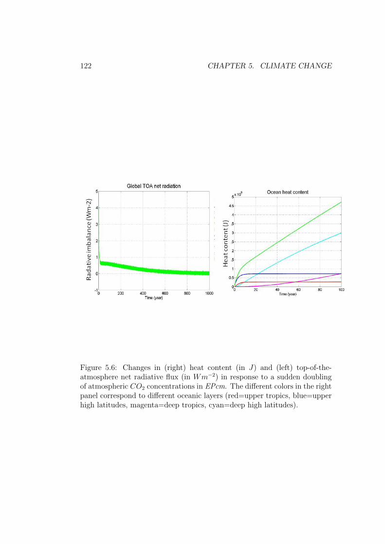
122 CHAPTER 5. CLIMATE CHANGE
Figure 5.6: Changes in (right) heat content (in J) and (left) top-of-the-atmosphere net radiative flux (in Wm−2) in response to a sudden doublingof atmospheric CO2 concentrations in EPcm. The different colors in the rightpanel correspond to different oceanic layers (red=upper tropics, blue=upperhigh latitudes, magenta=deep tropics, cyan=deep high latitudes).

5.3. CLIMATE CHANGE IN REALISTICMODELS ANDOBSERVATIONS123
The link between TOA radiative imbalance and ocean heat storage simplyreflects conservation of energy (Chapter 1):∫∫
∆FTOAdxdy =∂
∂t
∫∫∫ρoco∆Todxdydz + ... (5.5)
in which ∆FTOA is the net radiative imbalance at the TOA and ∆To is thechange in ocean temperature caused by doubling atmospheric CO2 concen-trations. Terms not explicitly written in this equation are the melting of thecryosphere, and the weak storage of heat in the atmosphere and land.
5.3 Climate change in realistic models and
observations
This section very briefly summarises the slides discussed in the last lecture.Regarding climate models:
• Climate models are numerical machines solving a large set of coupled,non linear, ordinary differential equations. Their main issue is the dif-ficult parameterization of processes occurring on a spatial scale smallerthan their grid size (clouds, convection, ocean turbulence, etc).
• In response to an increase in atmospheric CO2 concentration (and allother forcings discussed in Fig. 1), the models show an increase inglobal averaged surface temperature through time. The models allcapture the “troposphere warms / stratosphere cools” signature. Oceanwarming is sluggish and probably more diffusive in the models than inthe real world.
Concerning the observations:
• Observations do show the expected opposite temperature trends in thetroposphere and the stratosphere. The global averaged surface tem-perature has also increased since the beginning of the instruthe mentalrecord (early 20th century), with pronounced decadal timescale fluctu-ations.
• Top-of-the-atmosphere net radiative fluxes show an imbalance on theorder of +0.5Wm−2 since 2001 (net heating). This is, as expected,smaller than accounted for by anthropogenic forcing (Fig. 5.1) sincethis must account for the extra emission of infrared radiation by theocean+atmosphere (“the response” to anthropogenic forcing). Obser-vations of global ocean heat content agree with the TOA imbalancequalitatively and quantitatively.
124 CHAPTER 5. CLIMATE CHANGE
If you are interested to read more about the role of ocean heat uptake inthis problem, a recent and non technical summary is provided in Whitmarshet al. (2015).
Predictions of the 21st century climate rely entirely on climate models andas such can be debated and criticized at will because of the many imperfec-tions of the models. Likewise, all attempts to “prove” climate change throughanalysis of existing timeseries of surface temperature (and other relevant cli-matic timeseries) are endlessly subject to criticisms on statistical grounds.My personal take is that we can say something from first principles aboutthe timescales response to, and the magnitude of the forcing associated withanthropogenic accumulation of atmospheric carbon dioxide. The timescalesare mesmerizing: as we’ve seen in section 5.2, the interaction between theatmosphere and the ocean leads, at fixed atmospheric CO2 concentration, toadjustment times of several centuries; Earth system models with interactiveCO2 suggest adjustment times of several tens of thousands of years (Archer,2009). Thus it is not simply the climate we or our children live in which weare affecting. Overall, we should keep alive the “back-of-the-envelope” spirit:it shows that the current rate of accumulation of CO2 in the atmosphere isa major forcing in terms of rising sea level, melting of the cryosphere, etc(Czaja, 2012).
5.4 References
-Archer, D., 2009: “The Long Thaw: how humans are changing the next100,000 years of Earth’s climate”, Princeton University Press, 180pp.
-Bony et al., 2013: Robust direct effect of carbon dioxide on tropical circu-lation and regional precipitation, Nature Geoscience, 6, 447-451.
-Czaja, 2012: A consideration of the forcings of climate change using simplephysics, Discussion paper 2 of the Grantham Institute for Climate Change.
-Imbrie and Imbrie, 1979: “Ice ages, solving the mystery”, Harvard Univer-sity Press, 224 p.
-IPCC Fifth Assessment Report, 2013: please see Blackboard for a web linkto the various sections. If you have the stamina, this is an excellent sourceof information / figures for issues related to climate change.
-Lorenz, E. N., 1968: Climatic Determinism, AMS monograph, 8, 30, 1-3.
5.5. PROBLEMS 125
-Whitmarsh, et al., 2015: Ocean heat uptake and the global temperaturerecord, Grantham Institute briefing paper No 14.
5.5 Problems
Q1. Sea ice melting. Satellite observations suggest that the Earth hasbeen gaining 0.5Wm−2 of energy at the top-of-the-atmosphere since the early2000s. Estimate how long it would take to (i) melt Arctic sea ice (ii) increasethe temperature of the global ocean by 0.1K, were all this energy availableto do so. [Data: latent heat of fusion lf = 3 × 10⁵Jkg−1, ice density ρi =916kgm−3, ice thickness hi = 2m, ocean heat capacity co = 4000Jkg−1K−1,ocean density ρo = 1025kgm−3, average depth of the oceans ho = 3800m.]
Q2. Emission level. One way to think about the response of tropospherictemperature to a sudden increase in CO2 concentration is illustrated in Fig.1. Before the increase, the atmosphere effectively emits at a height ze, definedso that the total outgoing longwave radiation by the Earth (OLR) equalsσT (ze)
4 in which σ is Stefan-Boltzmann constant.
(i) Compute the emission level of the Earth, making a reasonable assump-tion regarding surface temperature and lapse-rate.
(ii) Explain why, as the CO2 concentration is suddenly doubled, the emis-sion level must increase.
(iii) Estimate this increase if, at equilibrium, the troposphere and the Earth’ssurface warm by 3K, assuming no change in lapse-rate.
(iv) The lapse-rate is empirically found to decrease with surface warmingin climate models. Would this tend to amplify the surface temperaturechange or to reduce it?
Q3. Clausius-Clapeyron scaling. From Thermodynamics (Year 2), thepressure of water vapour at equilibrium (denoted here by the symbol eeq)with liquid water satisfies, at a given temperature T ,
deeqdT
=sv − slvv − vl
(5.6)

126 CHAPTER 5. CLIMATE CHANGE
Figure 5.7: Schematic of temperature as a function of height, indicating theemission temperature and emission level. The outgoing longwave radiation(blue arrows) can be thought of originating from this level.

5.5. PROBLEMS 127
in which s is the specific entropy, v the specific volume and the subscripts land v refer to liquid and gas phases, respectively.
(i) Show that this can be rewritten as
deeqdT' lvTvv
(5.7)
stating any assumptions made.
(ii) Show that after using the ideal gas law this can be further rewrittenas,
deeqdT' eeqlvRvT 2
(5.8)
in which Rv = kB/mv, mv being the mass of a water molecule.
(iii) Use this expression to prove that equilibrium vapour pressure increasesby 7 % for every degree kelvin increase in temperature. [Data: lv =2.5 106Jkg−1, Rv = 461Jkg−1K−1].
Q4. Using the formula in Q3 from Chapter 4, discuss whether you agreewith the following statement taken from a popular science article about thevery anomalous 2013-2014 winter weather in the Northern Hemisphere:
“The Jet Stream is driven in part by the temperature difference between coldArctic air and the warmer air of the middle latitudes. Because the Arctic iswarming more rapidly than the rest of the planet, that difference is shrinking.This ought to produce a less potent Jet Stream.”
[Info: the polar warming amplification (≈ 1K) is restricted to a surface layerextending roughly from 1000hPa to 600hPa.]
Q5. Ocean heat uptake. We consider a “box-model” of the climate sys-tem to predict changes in top-of-the-atmosphere net radiative flux in re-sponse to a sudden increase in atmospheric CO2 concentrations. The oceanis decomposed into an upper (thickness h = 50m) and a deep layer (thick-ness H = 2000m). The density and specific heat of seawater are denotedby ρo = 1025kgm−3 and co = 4100Jkg−1K−1, respectively. At the top-of-the-atmosphere, the perturbation in the net radiative flux (positive down-wards) is written as N ′ = F ′ − αT ′ in which F ′ = 4Wm−2 for t > 0 (andF ′ = 0 for t < 0) is the anthropogenic forcing, T ′ is the global surface tem-perature anomaly, and α = 1.6Wm−2K−1 is the climate feedback parameter.

128 CHAPTER 5. CLIMATE CHANGE
Figure 5.8: Schematic of a box-model for ocean heat uptake O′.
(i) Find the timescale tu beyond which one can neglect the heat capacityof the upper ocean layer. Likewise, until which timescales td is the deepocean acting like a heat reservoir?
(ii) Discuss qualitatively and quantitatively the TOA radiative imbalanceon short timescales ( tu).
(iii) Climate models suggest that on intermediate timescales ( tu but td), the ocean heat uptake can be reasonably well modeled as O′ ≈κT ′ where κ = 0.5Wm−2K−1 is an “heat uptake efficiency”. Discussqualitatively and quantitatively the radiative imbalance at the TOA onthese timescales.
(iii) Discuss qualitatively and quantitatively the equilibrium state of themodel.

Chapter 6
Appendices
6.1 Radiative transfer
6.1.1 Radiation pencils vs. photon showers
You might have been wondering how to relate the concept of radiation in-tensity with the quantum physics ideas you’ve been learning so far. To doso, consider an horizontal plane and focus on computing the monochromaticirradiance across a surface area A (Fig. 6.1). In Chapter 2, we have beenwriting this as the integral of the radiation intensity Iλ over solid angle:
Fλ =
∫Iλ cos θdΩ (6.1)
A more intuitive view is to count photons with energy E such that hc/λ ≤E ≤ hc/λ + dE crossing the horizontal surface A per unit time. In thedirection making an angle θ with the vertical, these occupy the volume ofthe parallepiped of (slanted) side cdt. This volume is simply dV = Acdt cos θ.If nEdE denotes the number density of photons with the required energy, thenumber of photons contained in this volume is dN1:
dN1 = (Acdt cos θ)nEdE (6.2)
Now, all the photons in this volume do not travel towards the surface in thedirection θ. If we were in 1D, we would simply introduce a factor 1/2 at thisstage, to represent photons travelling upward or downward. In 3D, we use thesolid angle and write that in that volume dV only a fraction χdΩ/4π traveltowards the surface along the direction θ (if the radiation were isotropic wewould have χ = 1; if the radiation were entirely coming from the directionθ, we would have χdΩ/4π = δ(θ′ − θ) where the latter symbol reflects the
129

130 CHAPTER 6. APPENDICES
Figure 6.1: Calculation of the irradiance as a result of photons with energyE = hc/λ travelling from a given direction at speed c towards the surfaceA. This “photon shower” view contrasts with that of the “radiation pencil”illustrated in Fig. 2.4 in Chapter 2.
Dirac symbol). The number of photons travelling towards the surface alongthe direction θ and contained within the parallepiped is thus dN2:
dN2 = dN1χdΩ/4π = (Acdt cos θ)nEdEχdΩ/4π (6.3)
Since these all carry approximatively the energy E = hc/λ, the amount ofradiation energy through A per unit time, per unit energy interval is obtainedby summing over all parallepipeds. Let’s call this dFE:
dFE =∑
dN2E/(Adt) =
∫cEnEdEχ cos θdΩ/4π (6.4)
Physically, dFE represents exactly the same quantity as Fλdλ. Thus,(∫cEnEχ cos θdΩ/4π
)dE =
(∫Iλ cos θdΩ
)dλ (6.5)
Using the fact that |dE| = hcdλ/λ2, this suggests the following formula forthe intensity of radiation,
Iλ =χ
4π× (cnE
hc
λ2)× hc
λ(6.6)
I’ve written it as the product of three terms, to reflect more clearly its mean-ing. The first term is a geometric factor reflecting the geometry of the radia-tion. The second is the expected “transport” term considering that photons
6.2. THERMODYNAMICS OF MOIST AIR 131
travel at speed c and accounting for the conversion “per unit energy interval”to “per unit wavelength interval”. The last term is simply the energy of thephotons associated with the monochromatic radiation at wavelength λ.
6.1.2 Conservation of intensity
An interesting use of (6.6) is that the three terms identified on its righthand side are conserved if photons do not interact with matter (scattering,absorption). This is so because photons do not interact with each other sothat their statistics are unchanged in absence of scattering or absorption.This provides a straightforward explanation why Iλ is conserved in absenceof scattering or absorption.
6.1.3 Application to blackbody radiation
For this special case, we can use χ = 1 (isotropic) and also the result fromQuantum Physics (Year 2):
nE =8πE2
c3h3× 1
eE/kBT − 1(6.7)
Inserting this equation into (6.6), we recover eq. (2.1) in Chapter 2.
6.2 Thermodynamics of moist air
6.2.1 Entropy of cloudy air
We consider a sample of air in which vapour and liquid phases are assumedto be in equilibrium, i.e., e = eeq(T ) (RH = 1, see Fig. ??). If m denotesthe total mass of this sample, its specific entropy s satisfies,
ms = mdsd +mvsv +mlsl (6.8)
in which sd, sv and sl are the specific entropies for dry air, vapour and liquidwater, respectively. These are known functions of temperature and pressure:
sd = sd,ref + cp,d lnT
Tref−Rd ln
PdPref
(6.9)
sv = sv,ref + cp,v lnT
Tref−Rv ln
e
Pref(6.10)
132 CHAPTER 6. APPENDICES
and
sl = sl,ref + cl lnT
Tref(6.11)
(The constants Tref and Pref are arbitrary values where we assume we knowthe entropies).
Using the fact that on the vapour - liquid phase boundary sv − sl = lv/Twhere lv is the latent heat of vaporization, we have,
s = (1− qt)sd + qv(lvT
+ sl) + qlsl (6.12)
in which we have introduced the specific humidity qv, specific content ofliquid water ql and total specific content of water qt = qv + ql. Rearranging,
s = (1− qt)sd +lvqvT
+ qtsl (6.13)
After using the formulas for sd and sl, this can be rewritten as,
s = sref + [(1− qt)cp,d + qtcl] lnT
Tref− (1− qt)Rd ln
PdPref
+lvqvT
(6.14)
in which sref = (1− qt)sd,ref + qtsl,ref . Considering that qt 1, this formulacan be approximated as,
s ≈ sref + cp,d lnT
Tref−Rd ln
PdPref
+lvqvT
(6.15)
which is the form used in Chapter 3.
6.2.2 A general formula for the Brunt-Vaisala frequency?
We will start from (3.5) and, to simply this expression further, we use thefact that α is a state function, i.e., a mathematical function of any twothermodynamic variables (this is only true because of our assumption ofthermodynamic equilibrium). Because of the additional assumption of isen-tropic ascent, entropy s is a natural choice. We’ll take pressure P (the totalpressure, P = Pd + e) as the other variable,
α = α(P, s) (6.16)
As a result, and assuming small perturbations,
αe − αp ≈(∂α
∂s
)P
(se − sp) (6.17)

6.3. DYNAMICS OF ROTATING FLUIDS 133
(the term involving pressure changes drops because of our assumption thatthe environment and the parcel are at the same pressure). Using one ofMaxwell’s relations, this can be rewritten as,
αe − αp ≈(∂T
∂P
)s
(se − sp) (6.18)
At this stage we haven’t actually used that sp = cst. Following the sameprocedure used in the dry case when we considered how θ is conserved by aparcel moving upwards or downwards, we write,
se − sp ≈dsedz
(zp − zo) (6.19)
As a result, the parcel’s motion obeys,
d2zpdt2
= − g
αe
(∂T
∂P
)s
dsedz
(zp − zo) (6.20)
showing that the Brunt-Vaisala frequency is,
N2 =g
αe
(∂T
∂P
)s
dsedz
(6.21)
Stepping back from all this Thermodynamic, we realize that we haveactually not explicitly introduced moisture here –the above derivation is en-tirely general. For example, in the case of pure dry air (P = Pd), we recover(3.13) by using s = cp,d log θ, and (∂T/∂P )sd = αd/cp,d (since for dry air,ds = cp,ddT/T −RddP/P and Pdαd = RdT from the ideal gas law).
Acknowledging that at constant entropy, temperature always increaseswith pressure ((∂T/∂P )s > 0), (6.21) provides a fairly simple rule to testthe stability of a temperature profile (for the case of either pure dry air, orcloudy air in thermodynamic equilibrium): the profile is stable only if theentropy increases with height.
6.3 Dynamics of rotating fluids
6.3.1 Formula for D/Dt in a change of frame of refer-ence
Consider any vector A, which can be written in either an inertial frame withorthonormal axes (iI , jI ,kI), or in a rotating frame with orthonormal axes(iR, jR,kR),
A = Ax,IiI + Ay,IjI + Az,IkI = Ax,RiR + Ay,RjR + Az,RkR (6.22)

134 CHAPTER 6. APPENDICES
Taking the (D/Dt)I of this equation, that is the rate of change of vector Ain the inertial frame, we have,(
DA
Dt
)I
=
(DAx,IDt
)I
iI +
(DAy,IDt
)I
jI +
(DAz,IDt
)I
kI (6.23)
[NB: were we to take (DA/Dt)R we would obtain (DA/Dt)R = (DAx,R/Dt)RiR+(DAy,R/Dt)RjR + (DAz,R/Dt)RkR since the axes (iR, jR,kR) do not movein the rotating frame.]
Equation (6.23) is also,(DA
Dt
)I
=
(DAx,RiRDt
)I
+
(DAy,RjR
Dt
)I
+
(DAz,IkRDt
)I
(6.24)
The r.h.s can be further expanded using the product rule, for example forthe 1st term: (
DAx,RiRDt
)I
= Ax,R
(DiRDt
)I
+
(DAx,RDt
)I
iR (6.25)
Using (4.10), this is also,(DAx,RiRDt
)I
= Ax,R
(DiRDt
)I
+
(DAx,RDt
)R
iR (6.26)
hence:(DA
Dt
)I
=
(DA
Dt
)R
+ Ax,R
(DiRDt
)I
+ Ay,R
(DjRDt
)I
+ Az,R
(DkRDt
)I
(6.27)For the choice of a rotating frame centred at the Earth’s core, with kR = kI(parallel to the axis of rotation of the Earth) and (iR, jR) rotating at theangular velocity of the Earth Ω = 2π/1day, we obtain,(
DA
Dt
)I
=
(DA
Dt
)R
+ Ω×A (6.28)
since (DiR/Dt)I = Ω× iR, (DjR/Dt)I = Ω× jR and (DkR/Dt)I = 0 .
6.3.2 Kelvin’s identity
The rate of change of the contribution uI .ds of a small part of the circuit ineq. (4.57) can be written as,
D
Dt(uδx+ vδy+wδz) =
Du
Dtδx+
Dv
Dtδy+
Dw
Dtδz+ uδu+ vδv+wδw (6.29)
6.3. DYNAMICS OF ROTATING FLUIDS 135
in which, in this section only, we denote by u, v, w the velocities in the inertialframe and x, y, z the associated coordinates. It follows that for any segmentof the circuit, (
D
Dt
∫uI .ds
)I
=
∫ (DuIDt
)I
.ds+ [1
2u2I ], (6.30)
where the last term is the difference in the values between the end points.For a closed circuit this term vanishes, leading to eq. (4.57).
6.3.3 The vorticity equation?
To obtain an equation for the vorticity vector ζ (all components, not onlyits vertical component), “all you need” is to take the curl of (4.15), and usevector identities. In practice though, it is pretty tedious and so, to do thisin an efficient way though we need to a little bit of preparatory work. First,we rewrite (4.15) as,
∂uR∂t
+ (uR.∇)uR = −∇Φ− α∇P − 2Ω× uR + F fric (6.31)
Then we use the following vector identity,
∇(A.B) = (A.∇)B + (B.∇)A+A× (∇×B) +B × (∇×A) (6.32)
to obtain,
∂uR∂t
+ (2Ω + ζ)× uR = −∇(Φ + u2R/2)− α∇P + F fric (6.33)
The quantity 2Ω + ζ that appears in this equation requires a physical in-terpretation. It is the sum of the vorticity of the relative flow (ζ) and thevorticity of the solid body rotation at angular velocity Ω. We will call it fromnow on the absolute vorticity,
ζa ≡ 2Ω + ζ (6.34)
and measures the total local spin (planetary + relative) of a fluid parcel –see the discussion in Section 1.3.2. Typically in a cyclone, the relative andplanetary vorticity add up, so the total spin can be quite large. They tendto cancel each other in anticyclones.
To see where the 2Ω comes from, acknowledge that the velocity of theEarth’s solid body rotation is Ω × r = Ωr cosφi, so that it is a functionof latitude and radius r = R + z. As discussed in the lecture, the gradient

136 CHAPTER 6. APPENDICES
(or shear) in velocity associated with the variations with latitude (φ) addsup to the shear introduced by the variations with r to produce a planetaryvorticity vector always parallel to Ω. To be more quantitative one needs todo the math properly. A simple derivation is to compute ∇ × (Ω × r) in aCartesian coordinate system centred at the Earth’s core (since the curl of avector must be independent of the coordinate system used to compute it, wemight as well use the simplest coordinate system –we’ll denote it by i′, j ′,k′,the latter being parallel to Ω). Using the vector identity,
∇× (A×B) = A(∇.B)−B(∇.A) + (B.∇)A− (A.∇)B (6.35)
this becomes ∇ × (Ω × r) = Ω(∇.r) − r(∇.Ω) + (r.∇)Ω − (Ω.∇)r. Thesecond and third terms are zero because Ω is a constant vector. Since ∇.r =3 and (Ω.∇)r = Ω∂(zk′)/∂z = Ω, we get ∇× (Ω× r) = 3Ω−Ω = 2Ω.
We are now ready to take the curl of (6.33). Note first that the first termon the r.h.s. of (6.33) will not contribute since ∇ × ∇ = 0. So we simplyhave,
∂ζa∂t
+ ∇× (ζa × uR) = ∇× (−α∇P + F fric) (6.36)
where we have also used ∂ζa/∂t = ∂ζ/∂t. This can be simplified further byusing (6.35) to produce,(
DζaDt
)R
+ ζa(∇.uR)− (ζa.∇)uR = ∇× (−α∇P + F fric) (6.37)
At first sight this looks more complicated, but using the continuity equation(4.26), the first two terms on the l.h.s combine to produce,(
D
Dt(ζaρ
)
)R
− (ζaρ.∇)uR = α∇× (−α∇P + F fric) (6.38)
The first term on the r.h.s can also be simplified by using the vector identity,
∇× (A∇B) = ∇A×∇B (6.39)
to produce,(D
Dt(ζaρ
)
)R
= (ζaρ.∇)uR −
∇α×∇P
ρ+
∇× F fric
ρ(6.40)
or, after multiplication by ρ:
ρ
(D
Dt(αζa)
)R
= (ζa.∇)uR −∇α×∇P + ∇× F fric (6.41)