Notes on Becker and Lewis (1973)

On the Interaction between the Quantityand Quality of Children

Debreu Team1

Presented by Justina Adamanti, Liz Malm, Yuqing Hu, Krishanu A. Ray

Background

The trade-off between quantity and quality is a much-discussed issue ineconomics. In recent decades, economists have increasingly turned theirattention to behavior within families because of its direct implications forsuch diverse issues such as population growth, intergenerational transfersof wealth, human capital accumulation, and macroeconomic policy. In apioneering paper written by Gary S. Becker (1960), an economic frameworkis built by analyzing the factors that determine fertility, in which childrenare viewed as a durable goods that yield income to parents. Becker main-tains that the quality of children is directly related to the amount spenton them, and the number of children desired is directly related to income.Furthermore, many empirical studies performed in the past have demon-strated that quantity and quality of children within a given family oftenhave a negative correlation. Based on this, the Becker and Lewis (1973)paper (that we will present) further explores the interaction between quan-tity and quality of children. Becker and Lewis explain why the quantityand quality of children are “more closely related than any two commoditieschosen at random”(279). An increase in the quantity of children raises theshadow price (marginal cost) of the quality of children (and vice versa) andit demonstrates that the observed income elasticity of demand with respectto quality of children exceeds income elasticity with respect to quantity,while at the same time the observed price elasticity with respect to quantityis greater than price elasticity with respect to quality.

This paper was published in a special volume of Journal of Political Economy(Vol 81, part 2: New Economic Approaches to Fertility, 1973). Other papersin the volume are also emphasized in the Becker and Lewis article regardingtheir perspective on children and their quantity and quality trade-off, boththeoretically and empirically (such as Schultz, 1973, and Willis, 1973).

1In this handout, the equation labeling system in this handout can be explained asfollows: integers are the equations taken directly from the paper; letters denote equationsthat used in the derivations of the integer-labeled equations in the paper; and labels ofthe form A1, A2, etc. come from the mathematical appendix at the end of the paper.

1

The goal of this paper is to tease out and examine the relationship betweenquantity and quality of children, and to derive and understand the incomeand price elasticities with respect to both quantity and quality. Overall, thepaper argues that the crux of the interaction between quantity and qualityof children is a result of the fact that the marginal cost of quality is par-tially determined by quantity, and the marginal cost of quantity is partiallydetermined by quality. The two are inextricably linked.

What is the precise definition of quality of children? This differs basedon context. Two families living in different socioeconomic conditions mayhave very different ideas of what it means to increase the quality of theirchildren. Differing cultures could also change the context, in addition toa variety of demographic and psychological factors. For example, a familyliving in a developing country with little income may measure quality bythe amount of calories they are able to feed their children. An upper-middleclass American family may quantify quality by the years of college and grad-uate school they are able to provide for their children. It is not an explicitlydefined variable, because it differs based on situation.

The Model

Initial assumptions: No assumptions are made about the “closeness”of therelationship between quantity or quality (other authors make assumptionsregarding these variables, but Becker and Lewis do not); quality of childrenwithin the family is assumed to be identical for all children; parents makedecisions about n and q together and decide optimal n and q at the sametime; static optimization; and only parents determine quality, not other chil-dren (siblings) or child ability.

For a complete list of variables, see the end of this packet.

The authors identify three “goods”that give a family utility: the quantity ofchildren they have, n; the quality of their children (“as perceived by othersif not by the parents”themselves (279)), q; and the rate of all other com-modities consumed by the family, y.

A family has the following utility function,

U = U(n, q, y) (1)

and budget constraint,I = nqπ + yπy (2)

where I is the full money income of the family, π is the price of nq, andπy is the price of y. Note that it involves the assumption that n and q has

2

equal elasticity. The authors indicate that π is the price of nq, so nqπ canbe interpreted as the observed total expenditure on children by the family,which is determined by both quantity and quality.

Like any rational being, the family maximizes its utility subject to the bud-get constraint. Below we use the Lagrangian multiplier method to set up asimple static optimization problem.

Objective Function

L = U(n, q, y) + λ(I − nqπ − yπy) (a)

First Order Conditions

∂L

∂n=∂U

∂n− λnπ = 0 (b)

∂L

∂q=∂U

∂n− λqπ = 0 (c)

∂L

∂y=∂U

∂n− λyπ = 0 (d)

∂L

∂λ= I − nqπ − yπy = 0 (e)

Thus, the utility maximizing conditions, taking into account the family’sbudget constraint, are where marginal utility of n, q, and y equal themarginal cost of n, q, and y, respectively.

MUn = λqπ = λpn

MUq = λnπ = λpq (3)

MUy = λyπ = λpy,

Here, λ is the marginal utility of money income, MUn is the marginal util-ity obtained from having an extra child, pn is the marginal cost of havingan additional child, MUq is the marginal utility from increasing the qualityof each child in the family by one unit, pq is the marginal cost (marginalcosts will also be referred to as shadow prices) of increasing the quality ofeach child in the family by one unit, MUy is the marginal utility obtainedfrom increasing consumption of y by one unit, and py is the marginal costof increasing consumption of y by one unit.

From the above three equations, we can see that the marginal costs (alsoreferred to as shadow prices) of each good are as follows:

pn = qπ

3

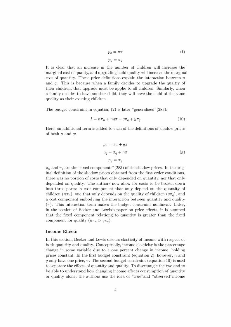
pq = nπ (f)

py = πy

It is clear that an increase in the number of children will increase themarginal cost of quality, and upgrading child quality will increase the marginalcost of quantity. These price definitions explain the interaction between nand q. This is because when a family decides to upgrade the qualtiy oftheir children, that upgrade must be applie to all children. Similarly, whena family decides to have another child, they will have the child of the samequality as their existing children.

The budget constraint in equation (2) is later “generalized”(283):

I = nπn + nqπ + qπq + yπy (10)

Here, an additional term is added to each of the definitions of shadow pricesof both n and q:

pn = πn + qπ

pq = πq + nπ (g)

py = πy

πn and πq are the “fixed components”(283) of the shadow prices. In the orig-inal definition of the shadow prices obtained from the first order conditions,there was no portion of costs that only depended on quantity, nor that onlydepended on quality. The authors now allow for costs to be broken downinto three parts: a cost component that only depend on the quantity ofchildren (nπn), one that only depends on the quality of children (qπq), anda cost component embodying the interaction between quantity and quality(π). This interaction term makes the budget constraint nonlinear. Later,in the section of Becker and Lewis‘s paper on price effects, it is assumedthat the fixed component relationg to quantity is greater than the fixedcomponent for quality (nπn > qπq).

Income Effects

In this section, Becker and Lewis discuss elasticity of income with respect otboth quantity and quality. Conceptually, income elasticity is the percentagechange in some variable due to a one percent change in income, holdingprices constant. In the first budget constraint (equation 2), however, n andq only have one price, π. The second budget constraint (equation 10) is usedto separate the effects of quantity and quality. To disentangle the two and tobe able to understand how changing income affects consumption of quantityor quality alone, the authors use the idea of “true”and “observed”income

4

elasticities by using two different measures of income and two different typesof prices.

True and observed income elasticities differ because they each use a dif-ferent definition of “income”and “price”. Becker and Lewis assume thattrue income elasticity with respect to quality is larger than with respect toquantity. Before proving that the assumption also applies to observed elas-ticities, they prove that there exists a difference between true and observedelasticities (the “downward bias”). They also show that the “downwardbias”(281) in the observed elasticities and the effect on price can result theobserved elasticity for quantity being negative even though the true elastic-ity for quantity is not.

We know that I=W , and W = wp, where W is nominal wage, and w isreal wage, and p is the price level, so when I increases, it means there isan increase in W . However, the increase in ratio terms, is less in real in-come than money income, because the costs of producing commodities inthe household are increased by th rise in the price of time (281), we knowthe increase in I is larger than the increase in w, since I = wp, it must bethat p also increases. Thus we know the price level increases, so pn and pqalso increase, which would lead to the decrease in n and q.

True Income Elasticities

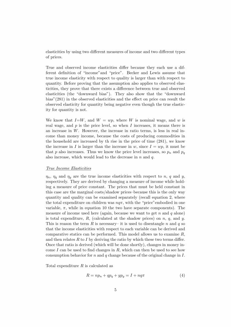
ηn, ηq and ηy are the true income elasticities with respect to n, q and y,respectively. They are derived by changing a measure of income while hold-ing a measure of price constant. The prices that must be held constant inthis case are the marginal costs/shadow prices–because this is the only wayquantity and quality can be examined separately (recall equation 2, wherethe total expenditure on children was nqπ, with the “price”embodied in onevariable, π, while in equation 10 the two have separate components). Themeasure of income used here (again, because we want to get n and q alone)is total expenditure, R, (calculated at the shadow prices) on n, q, and y.This is reason the term R is necessary– it is used to disentangle n and q sothat the income elasticities with respect to each variable can be derived andcomparative statics can be performed. This model allows us to examine R,and then relates R to I by deriving the ratio by which these two terms differ.Once that ratio is derived (which will be done shortly), changes in money in-come I can be used to find changes in R, which can then be used to see howconsumption behavior for n and q change because of the original change in I.

Total expenditure R is calculated as

R = npn + qpq + ypy = I + nqπ (4)

5

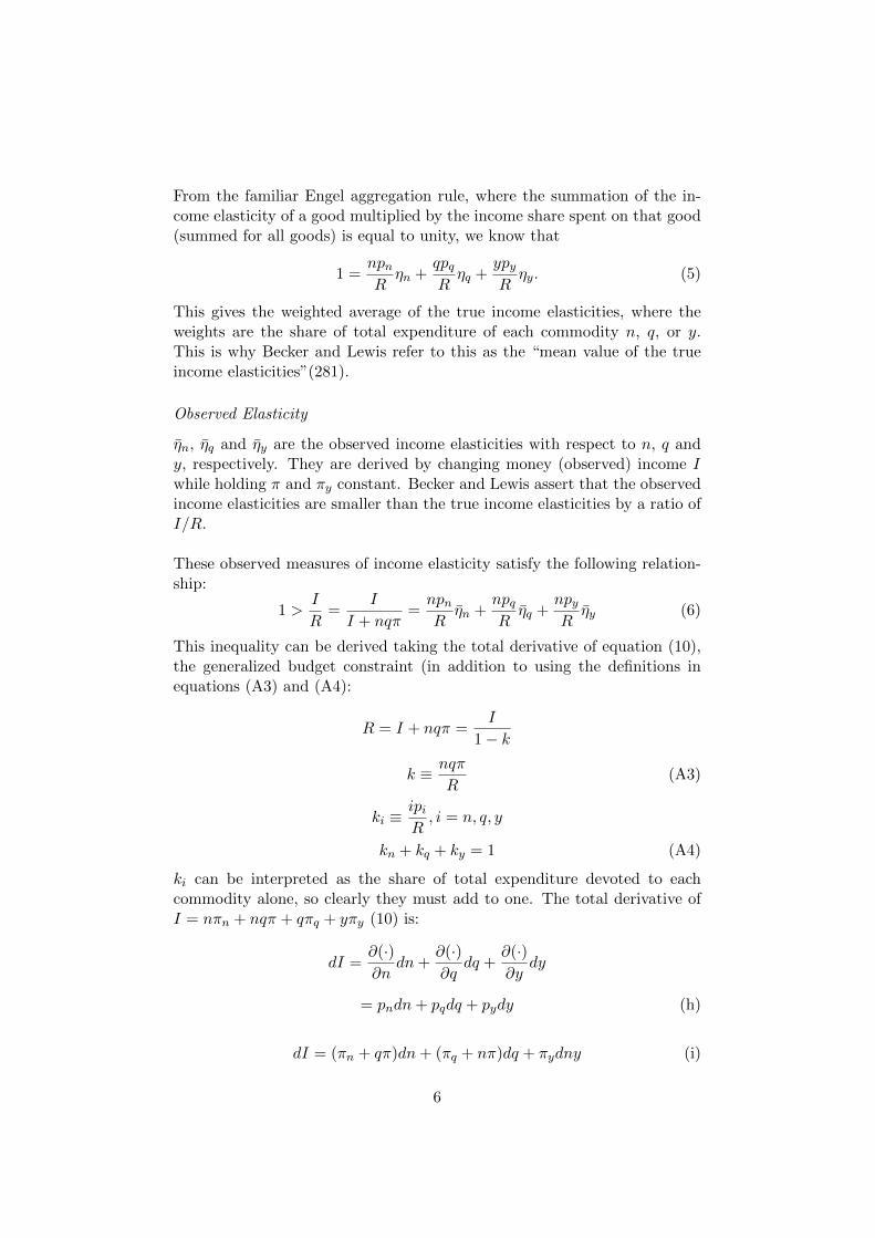
From the familiar Engel aggregation rule, where the summation of the in-come elasticity of a good multiplied by the income share spent on that good(summed for all goods) is equal to unity, we know that

1 =npnR

ηn +qpqRηq +

ypyRηy. (5)

This gives the weighted average of the true income elasticities, where theweights are the share of total expenditure of each commodity n, q, or y.This is why Becker and Lewis refer to this as the “mean value of the trueincome elasticities”(281).

Observed Elasticity

η̄n, η̄q and η̄y are the observed income elasticities with respect to n, q andy, respectively. They are derived by changing money (observed) income Iwhile holding π and πy constant. Becker and Lewis assert that the observedincome elasticities are smaller than the true income elasticities by a ratio ofI/R.

These observed measures of income elasticity satisfy the following relation-ship:

1 >I

R=

I

I + nqπ=npnR

η̄n +npqRη̄q +

npyRη̄y (6)

This inequality can be derived taking the total derivative of equation (10),the generalized budget constraint (in addition to using the definitions inequations (A3) and (A4):

R = I + nqπ =I

1− k

k ≡ nqπ

R(A3)

ki ≡ipiR, i = n, q, y

kn + kq + ky = 1 (A4)

ki can be interpreted as the share of total expenditure devoted to eachcommodity alone, so clearly they must add to one. The total derivative ofI = nπn + nqπ + qπq + yπy (10) is:

dI =∂(·)∂n

dn+∂(·)∂q

dq +∂(·)∂y

dy

= pndn+ pqdq + pydy (h)

dI = (πn + qπ)dn+ (πq + nπ)dq + πydny (i)

6

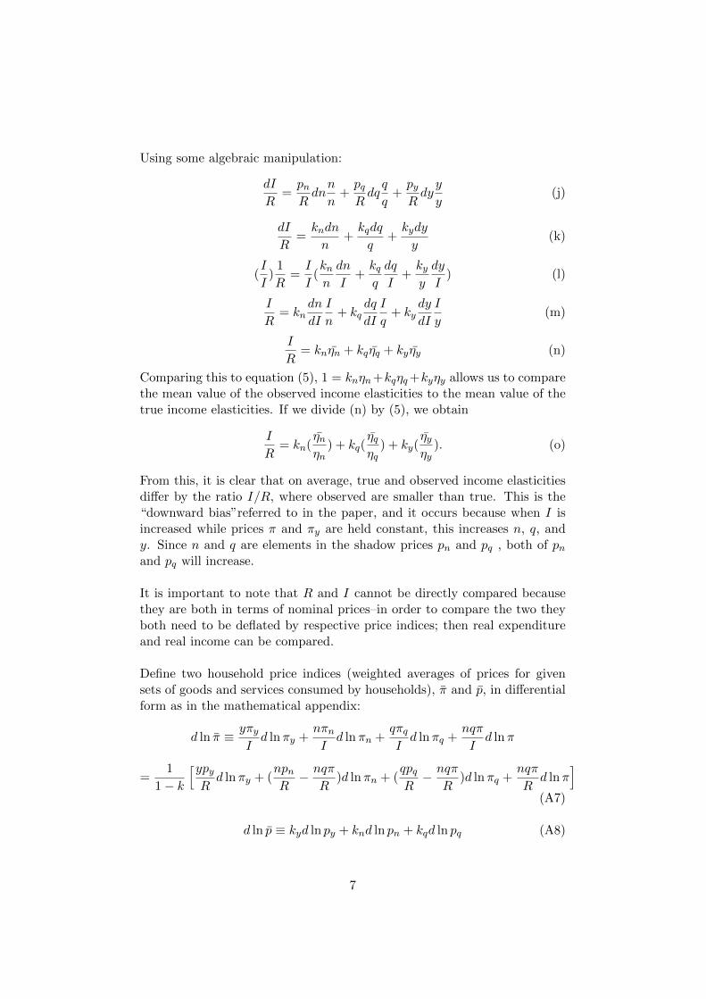
Using some algebraic manipulation:

dI

R=pnRdnn

n+pqRdqq

q+pyRdyy

y(j)

dI

R=kndn

n+kqdq

q+kydy

y(k)

(I

I)

1

R=I

I(knn

dn

I+kqq

dq

I+kyy

dy

I) (l)

I

R= kn

dn

dI

I

n+ kq

dq

dI

I

q+ ky

dy

dI

I

y(m)

I

R= knη̄n + kqη̄q + kyη̄y (n)

Comparing this to equation (5), 1 = knηn+kqηq+kyηy allows us to comparethe mean value of the observed income elasticities to the mean value of thetrue income elasticities. If we divide (n) by (5), we obtain

I

R= kn(

η̄nηn

) + kq(η̄qηq

) + ky(η̄yηy

). (o)

From this, it is clear that on average, true and observed income elasticitiesdiffer by the ratio I/R, where observed are smaller than true. This is the“downward bias”referred to in the paper, and it occurs because when I isincreased while prices π and πy are held constant, this increases n, q, andy. Since n and q are elements in the shadow prices pn and pq , both of pnand pq will increase.

It is important to note that R and I cannot be directly compared becausethey are both in terms of nominal prices–in order to compare the two theyboth need to be deflated by respective price indices; then real expenditureand real income can be compared.

Define two household price indices (weighted averages of prices for givensets of goods and services consumed by households), π̄ and p̄, in differentialform as in the mathematical appendix:

d ln π̄ ≡ yπyId lnπy +

nπnId lnπn +

qπqId lnπq +

nqπ

Id lnπ

=1

1− k

[ypyRd lnπy + (

npnR− nqπ

R)d lnπn + (

qpqR− nqπ

R)d lnπq +

nqπ

Rd lnπ

](A7)

d ln p̄ ≡ kyd ln py + knd ln pn + kqd ln pq (A8)

7

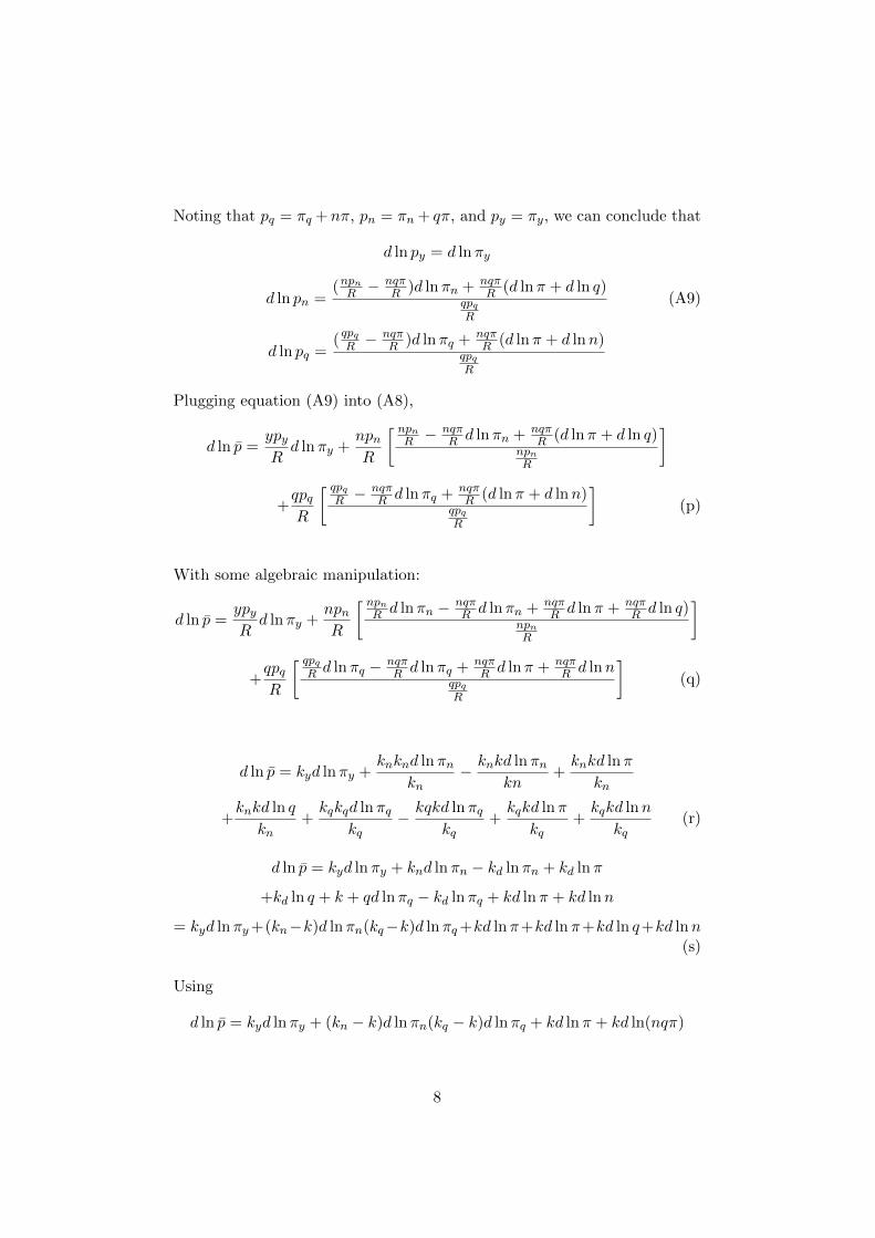
Noting that pq = πq +nπ, pn = πn + qπ, and py = πy, we can conclude that

d ln py = d lnπy

d ln pn =(npnR −

nqπR )d lnπn + nqπ

R (d lnπ + d ln q)qpqR

(A9)

d ln pq =(qpqR −

nqπR )d lnπq + nqπ

R (d lnπ + d lnn)qpqR

Plugging equation (A9) into (A8),

d ln p̄ =ypyRd lnπy +

npnR

[ npnR −

nqπR d lnπn + nqπ

R (d lnπ + d ln q)npnR

]

+qpqR

[ qpqR −

nqπR d lnπq + nqπ

R (d lnπ + d lnn)qpqR

](p)

With some algebraic manipulation:

d ln p̄ =ypyRd lnπy +

npnR

[ npnR d lnπn − nqπ

R d lnπn + nqπR d lnπ + nqπ

R d ln q)npnR

]

+qpqR

[ qpqR d lnπq − nqπ

R d lnπq + nqπR d lnπ + nqπ

R d lnnqpqR

](q)

d ln p̄ = kyd lnπy +knknd lnπn

kn− knkd lnπn

kn+knkd lnπ

kn

+knkd ln q

kn+kqkqd lnπq

kq− kqkd lnπq

kq+kqkd lnπ

kq+kqkd lnn

kq(r)

d ln p̄ = kyd lnπy + knd lnπn − kd lnπn + kd lnπ

+kd ln q + k + qd lnπq − kd lnπq + kd lnπ + kd lnn

= kyd lnπy+(kn−k)d lnπn(kq−k)d lnπq+kd lnπ+kd lnπ+kd ln q+kd lnn(s)

Using

d ln p̄ = kyd lnπy + (kn − k)d lnπn(kq − k)d lnπq + kd lnπ + kd ln(nqπ)

8

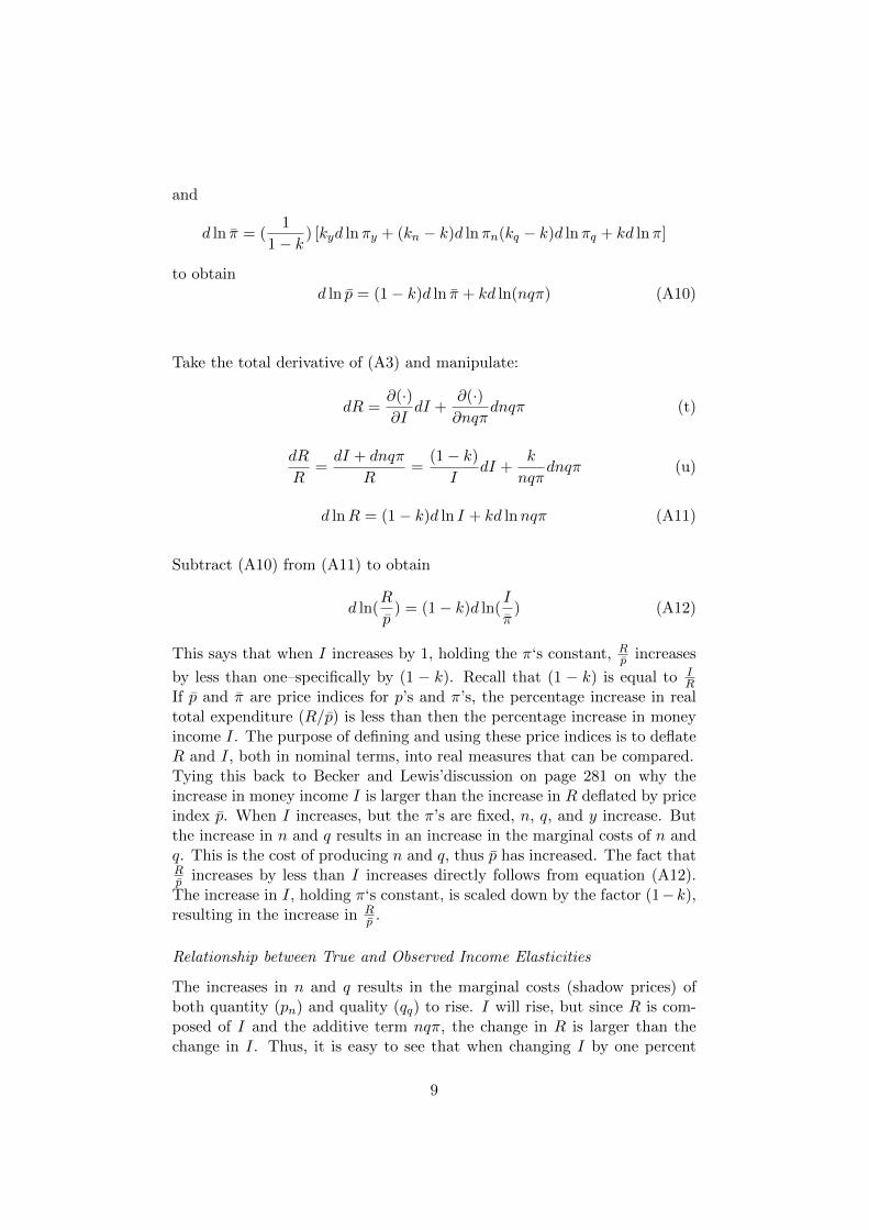
and

d ln π̄ = (1

1− k) [kyd lnπy + (kn − k)d lnπn(kq − k)d lnπq + kd lnπ]

to obtaind ln p̄ = (1− k)d ln π̄ + kd ln(nqπ) (A10)

Take the total derivative of (A3) and manipulate:

dR =∂(·)∂I

dI +∂(·)∂nqπ

dnqπ (t)

dR

R=dI + dnqπ

R=

(1− k)

IdI +

k

nqπdnqπ (u)

d lnR = (1− k)d ln I + kd lnnqπ (A11)

Subtract (A10) from (A11) to obtain

d ln(R

p̄) = (1− k)d ln(

I

π̄) (A12)

This says that when I increases by 1, holding the π‘s constant, Rp̄ increases

by less than one–specifically by (1 − k). Recall that (1 − k) is equal to IR

If p̄ and π̄ are price indices for p’s and π’s, the percentage increase in realtotal expenditure (R/p̄) is less than then the percentage increase in moneyincome I. The purpose of defining and using these price indices is to deflateR and I, both in nominal terms, into real measures that can be compared.Tying this back to Becker and Lewis’discussion on page 281 on why theincrease in money income I is larger than the increase in R deflated by priceindex p̄. When I increases, but the π’s are fixed, n, q, and y increase. Butthe increase in n and q results in an increase in the marginal costs of n andq. This is the cost of producing n and q, thus p̄ has increased. The fact thatRp̄ increases by less than I increases directly follows from equation (A12).The increase in I, holding π‘s constant, is scaled down by the factor (1−k),resulting in the increase in R

p̄ .

Relationship between True and Observed Income Elasticities

The increases in n and q results in the marginal costs (shadow prices) ofboth quantity (pn) and quality (qq) to rise. I will rise, but since R is com-posed of I and the additive term nqπ, the change in R is larger than thechange in I. Thus, it is easy to see that when changing I by one percent

9

but holding marginal costs constant (p), we obtain the percentage change inn, q, and y, which will be less than the effect of changing R by one percentand holding the ps constant (gives us the percentage change in n, q, and yfrom a one percent change in I–the true income elasticities).

The authors assert that “the true income elasticity with respect to qual-ity is substantially larger than that with respect to quantity,”i.e. ηq > ηn.That is, when a family’s income changes, the resulting percentage change inquality is much larger than the change in quantity. Families may choose onlyto increase quality of their children, while refraining from having additionalchildren. This could be due to circumstances or preferences: it is easy to seewhy investing more in your existing children would be more desirable (andperhaps even easier) than having another child. Perhaps the fixed costs ofn are much larger than the fixed costs of q.

Furthermore, “because of the downward bias in the observed elasticities andthe effect on prices, the observed elasticity for quantity may be negative eventhough the true elasticity is not”(page 281). That is, an increase in moneyincome I could cause a family to increase the quality of their children, butnot have any more children (because a family cannot “decrease”consumptionof n and just get rid of one of their children). Theoretically, however, thefollowing results: if the true income elasticity with respect to quantity iszero (ηn = 0) and I increases while prices π and πy are held constant, thiswill cause no change in n initially and will cause q and y to increase. Butthese increases in q and y will cause the shadow price of n to increase (re-call that pn = πn + qπ) relative to the other two goods since the shadowprices of quality and y do not rise, and families will substitute away fromthe consumption of n (although in reality this cannot occur - once you havechildren you are stuck with them!). This shows that even though the trueincome elasticity with respect to quantity may be zero, n still may declinewith a rise in I simply because the marginal cost of q decreases, of which nis a component.

The third part of the appendix (begining on page 286 with, “We now turn tothe derivation of...”) is used to derive both observed substitution elasticityand observed income elasticity with respect to both q and n and comparethe two. It follows from (A9), below,

d ln py = d lnπy

d ln pn = d ln(kn − k)d lnπn + k(d lnπ + d ln q)

kn(A9)

d ln pq = d ln(kq − k)d lnπq + k(d lnπ + d lnn)

kq

10

and the fact that we can change I while the π’s are held constant that

d ln(R

p̄) = (1− k)d ln(

I

π̄). (A12)

This follows directly from the assumption that theπ’s are held constant, sofrom (A9) and (A12) we find

d ln py = 0

d ln pn =kd ln q

kn

d ln pq =kd lnn

kq(A14)

d ln(R

p̄) = (1− k)d ln(1− k)

This final equation says that as I changes by one, the real expenditure, (Rp̄ )changes by less than one, specifically (1 − k). Equations (A13) and (A14)can be substituted into one another and terms can be collected to produce(A15) and (A16). (Note: this is a lot of messy algebra; if anyone would liketo see the derivations, ask one of the group members.) Note that (A16) isjust a more general version of equations (7) and (8) below, which can bederived by assuming that kq=kn=k. (Note that the budget constraint thatonly contains the interaction term (2) is utilized, rather than the generalizedbudget constraint (10).)

Dη̄n1− k

= (1− kσnq)ηn − (1− k)σ̄nηq

Dη̄q1− k

= (1− kσnq)ηq − (1− k)σ̄qηn (7)

where k ≡ nqπ

R

(1− k)σ̄n = kσnq + (1− 2k)σny

(1− k)σ̄q = kσnq + (1− 2k)σqy

D ≡ (1− kσnq)2 − (1− k)2σ̄nσ̄q

(8)

D

1− k(η̄q = η̄n) = ηq − ηn + (1− 2k)(σnyηq − σqyηn) (9)

From equation (7), we can see that even if ηn is positive, if the secondterm on the righthand side is larger than the first term, ηn may be negativebecause D and (1− k) are both greater than zero (and (1− kσnq) > 0 and

11

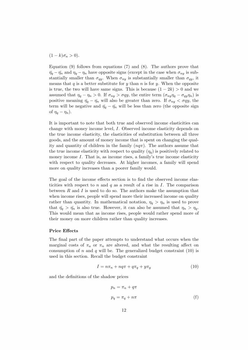
(1− k)σ̄n > 0).

Equation (9) follows from equations (7) and (8). The authors prove thatη̄q − η̄n and ηq − ηn have opposite signs (except in the case when σny is sub-stantially smaller than σqy. When σny is substantially smaller than σqy, itmeans that q is a better substitute for y than n is for y. When the oppositeis true, the two will have same signs. This is because (1 − 2k) > 0 and weassumed that ηq − ηn > 0. If σny > σqy, the entire term (σnyηq − σqyηn) ispositive meaning η̄q − η̄n will also be greater than zero. If σny < σqy, theterm will be negative and η̄q − η̄n will be less than zero (the opposite signof ηq − ηn).

It is important to note that both true and observed income elasticities canchange with money income level, I. Observed income elasticity depends onthe true income elasticity, the elasticities of substitution between all threegoods, and the amount of money income that is spent on changing the qual-ity and quantity of children in the family (nqπ). The authors assume thatthe true income elasticity with respect to quality (ηq) is positively related tomoney income I. That is, as income rises, a family’s true income elasticitywith respect to quality decreases. At higher incomes, a family will spendmore on quality increases than a poorer family would.

The goal of the income effects section is to find the observed income elas-ticities with respect to n and q as a result of a rise in I. The comparisonbetween R and I is used to do so. The authors make the assumption thatwhen income rises, people will spend more their increased income on qualityrather than quantity. In mathematical notation, ηq > ηn is used to provethat η̄q > η̄n is also true. However, it can also be assumed that ηn > ηq.This would mean that as income rises, people would rather spend more oftheir money on more children rather than quality increases.

Price Effects

The final part of the paper attempts to understand what occurs when themarginal costs of πa or πn are altered, and what the resulting affect onconsumption of n and q will be. The generalized budget constraint (10) isused in this section. Recall the budget constraint

I = nπn + nqπ + qπq + yπy (10)

and the definitions of the shadow prices

pn = πn + qπ

pq = πq + nπ (f)

12

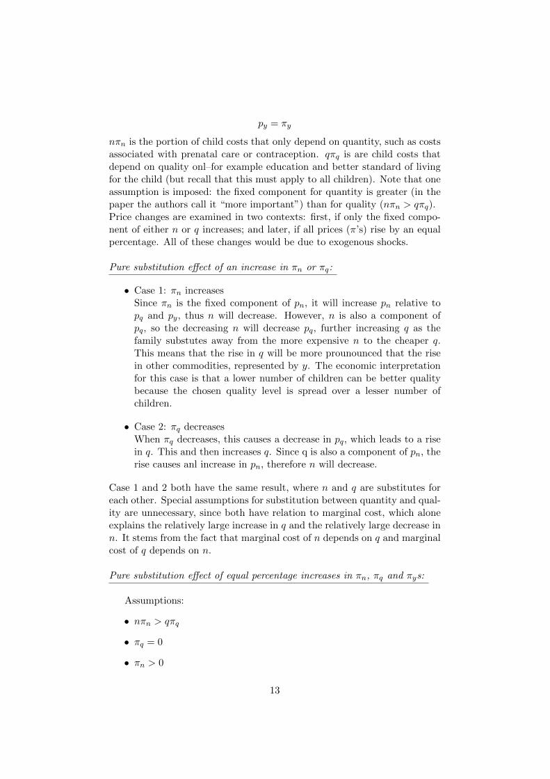
py = πy

nπn is the portion of child costs that only depend on quantity, such as costsassociated with prenatal care or contraception. qπq is are child costs thatdepend on quality onl–for example education and better standard of livingfor the child (but recall that this must apply to all children). Note that oneassumption is imposed: the fixed component for quantity is greater (in thepaper the authors call it “more important”) than for quality (nπn > qπq).Price changes are examined in two contexts: first, if only the fixed compo-nent of either n or q increases; and later, if all prices (π’s) rise by an equalpercentage. All of these changes would be due to exogenous shocks.

Pure substitution effect of an increase in πn or πq:

• Case 1: πn increasesSince πn is the fixed component of pn, it will increase pn relative topq and py, thus n will decrease. However, n is also a component ofpq, so the decreasing n will decrease pq, further increasing q as thefamily substutes away from the more expensive n to the cheaper q.This means that the rise in q will be more prounounced that the risein other commodities, represented by y. The economic interpretationfor this case is that a lower number of children can be better qualitybecause the chosen quality level is spread over a lesser number ofchildren.

• Case 2: πq decreasesWhen πq decreases, this causes a decrease in pq, which leads to a risein q. This and then increases q. Since q is also a component of pn, therise causes anl increase in pn, therefore n will decrease.

Case 1 and 2 both have the same result, where n and q are substitutes foreach other. Special assumptions for substitution between quantity and qual-ity are unnecessary, since both have relation to marginal cost, which aloneexplains the relatively large increase in q and the relatively large decrease inn. It stems from the fact that marginal cost of n depends on q and marginalcost of q depends on n.

Pure substitution effect of equal percentage increases in πn, πq and πys:

Assumptions:

• nπn > qπq

• πq = 0

• πn > 0

13

• n and q are equally good substitutes for y (have the same elasticity)

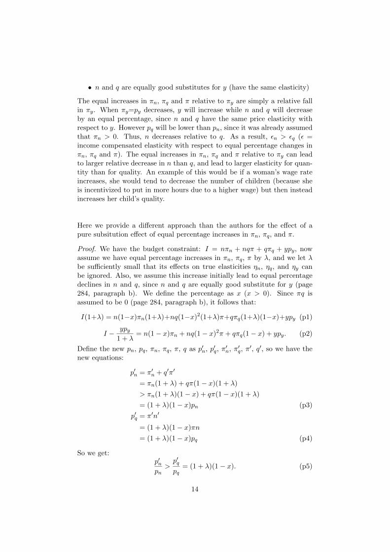
The equal increases in πn, πq and π relative to πy are simply a relative fallin πy. When πy=py decreases, y will increase while n and q will decreaseby an equal percentage, since n and q have the same price elasticity withrespect to y. However pq will be lower than pn, since it was already assumedthat πn > 0. Thus, n decreases relative to q. As a result, εn > εq (ε =income compensated elasticity with respect to equal percentage changes inπn, πq and π). The equal increases in πn, πq and π relative to πy can leadto larger relative decrease in n than q, and lead to larger elasticity for quan-tity than for quality. An example of this would be if a woman’s wage rateincreases, she would tend to decrease the number of children (because sheis incentivized to put in more hours due to a higher wage) but then insteadincreases her child’s quality.

Here we provide a different approach than the authors for the effect of apure subsitution effect of equal percentage increases in πn, πq, and π.

Proof. We have the budget constraint: I = nπn + nqπ + qπq + ypy, nowassume we have equal percentage increases in πn, πq, π by λ, and we let λbe sufficiently small that its effects on true elasticities ηn, ηq, and ηy canbe ignored. Also, we assume this increase initially lead to equal percentagedeclines in n and q, since n and q are equally good substitute for y (page284, paragraph b). We define the percentage as x (x > 0). Since πq isassumed to be 0 (page 284, paragraph b), it follows that:

I(1+λ) = n(1−x)πn(1+λ)+nq(1−x)2(1+λ)π+qπq(1+λ)(1−x)+ypy (p1)

I − ypy1 + λ

= n(1− x)πn + nq(1− x)2π + qπq(1− x) + ypy. (p2)

Define the new pn, pq, πn, πq, π, q as p′n, p′q, π′n, π′q, π

′, q′, so we have thenew equations:

p′n = π′n + q′π′

= πn(1 + λ) + qπ(1− x)(1 + λ)

> πn(1 + λ)(1− x) + qπ(1− x)(1 + λ)

= (1 + λ)(1− x)pn (p3)

p′q = π′n′

= (1 + λ)(1− x)πn

= (1 + λ)(1− x)pq (p4)

So we get:p′npn

>p′qpq

= (1 + λ)(1− x). (p5)

14

The initial change in n and q might not be equal to their eventual change,now assume the true percentage decrease in n and q are m and g, so againwe get:

1 =n(1−m)pn(1− a)

R′ηn +

q(1− g)pq(1− b)R′

ηq +ypyR′

ηy. (p14)

Note we hold the elasticities unchanged, since λ is small enough that elas-ticities are approximately equal to their original ones. Now we have:

n(1−m)pn(1− a)

R′ηn =

npnR

ηn, (p15)

q(1− g)pq(1− b)R′

ηq =qpqRηq, (p16)

we get1−m1− g

=1− b1− a

< 1, (p17)

som > g,

which means4nn

>4qq, (p18)

Thus we can see that the percentage decrease in quantity n is larger thanthat in quality q. This completes the proof.

Main Conclusions

• When a couple decides to have a family, they decide not only howmany children to raise, but what quality of children to have (Becker,1960). However, the family choice of the optimal number and qualityof children is not the focus of this paper, it builds upon past research inorder to explore and explain the behavior of child number and qualitywhen parameters such as income and “price”change.

• Quantity and quality are not exactly separable goods, because each“unit”of child embodies both. The quantity and quality are closelyrelated and can substitute each other, since they depend on each otherin their shadow prices.

• Observed income elasticity of q is greater than income elasticity for n,but the opposite is true for price elasticities.

• There is a downward bias of (1 − k) on observed income elasticities,when compared to true income elasticities.

15

Criticism

Though elegant as it stands, the model is too simple to explain the realworld. We come up with the following limits:

• First and foremost, the failure to explicitly define what is meant by”quality” makes initial conceptual understanding difficult.

• The authors assume that within the budget constraint any couple con-siders itself free to choose any combination it wishes of numbers of chil-dren and expenditure per child (prices of particular goods and servicesbeing given). However, in reality, the quantity and quality should havea lower and upper bound. Given the education level, occupation, re-gion and a few other factors, and the mundane (such as the “one-childpolicy”in China) and mechanical considerations, most couples wouldconsider that they have a very narrow range of choice.

• For consumer goods, quantity appears to be a closer substitute forquality than in the case of children. Two lower-price cars may beconsidered equivalent to one high-priced car for the high income family.However, is it unlikely that this family would be indifferent towardhaving two children who are untrained or not well-educated, or havingone well-educated child. In fact, some parents may derive disutility iftheir children fall below their quality standards, whatever those maybe.

• This model is restricted to static economic assumptions, from whichit nevertheless derives a good deal of analytical power; it cannot yet,however, cope adequately with the lifetime behavior of parents withrespect to the many diverse investments they make in the health, edu-cation, on-the-job training, travel, and marriage of their children andwith respect to the transfer of property via inheritance. It is alsounable to account for revisions of these expectations and for the ad-justments that parents make to unexpected income changes along thelife-cycle path. Quality increases in children require both time andmoney, and non-monetary costs must certainly be of some importancein determining family size. Regarding this, the effect of income onfamily size will be greatly weakened by the tendency for the standardof living for children to advance more or less proportionately with thatof the parents.

• This one-family model only considers the situation in which parentsspend money on their children, while ignorant of the fact that theparents are themselves the children of their older parents. Intergener-ational transfers are neglected, but Becker incorporates it in his laterpaper (interested readers may refer to Becker’s 1974 paper, “A Theoryof Social Interactions”).

16

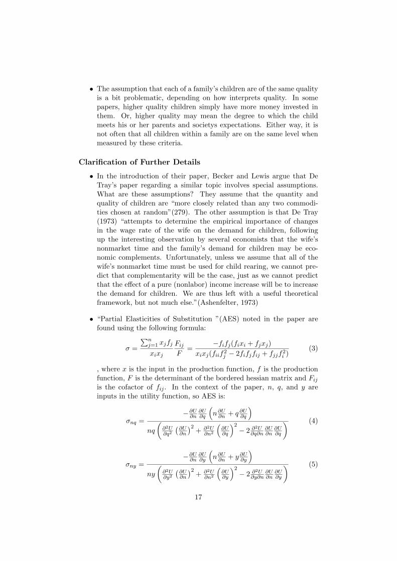
• The assumption that each of a family’s children are of the same qualityis a bit problematic, depending on how interprets quality. In somepapers, higher quality children simply have more money invested inthem. Or, higher quality may mean the degree to which the childmeets his or her parents and societys expectations. Either way, it isnot often that all children within a family are on the same level whenmeasured by these criteria.

Clarification of Further Details

• In the introduction of their paper, Becker and Lewis argue that DeTray’s paper regarding a similar topic involves special assumptions.What are these assumptions? They assume that the quantity andquality of children are “more closely related than any two commodi-ties chosen at random”(279). The other assumption is that De Tray(1973) “attempts to determine the empirical importance of changesin the wage rate of the wife on the demand for children, followingup the interesting observation by several economists that the wife’snonmarket time and the family’s demand for children may be eco-nomic complements. Unfortunately, unless we assume that all of thewife’s nonmarket time must be used for child rearing, we cannot pre-dict that complementarity will be the case, just as we cannot predictthat the effect of a pure (nonlabor) income increase will be to increasethe demand for children. We are thus left with a useful theoreticalframework, but not much else.”(Ashenfelter, 1973)

• “Partial Elasticities of Substitution ”(AES) noted in the paper arefound using the following formula:

σ =

∑nj=1 xjfj

xixj

FijF

=−fifj(fixi + fjxj)

xixj(fiif2j − 2fifjfij + fjjf2

i )(3)

, where x is the input in the production function, f is the productionfunction, F is the determinant of the bordered hessian matrix and Fijis the cofactor of fij . In the context of the paper, n, q, and y areinputs in the utility function, so AES is:

σnq =−∂U∂n

∂U∂q

(n∂U∂n + q ∂U∂q

)nq

(∂2U∂q2

(∂U∂n

)2+ ∂2U

∂n2

(∂U∂q

)2− 2 ∂2U

∂q∂n∂U∂n

∂U∂q

) (4)

σny =−∂U∂n

∂U∂y

(n∂U∂n + y ∂U∂y

)ny

(∂2U∂y2

(∂U∂n

)2+ ∂2U

∂n2

(∂U∂y

)2− 2 ∂2U

∂y∂n∂U∂n

∂U∂y

) (5)

17

σqy =−∂U∂q

∂U∂y

(q ∂U∂q + y ∂U∂y

)qy

(∂2U∂y2

(∂U∂q

)2+ ∂2U

∂q2

(∂U∂y

)2− 2 ∂2U

∂y∂q∂U∂q

∂U∂y

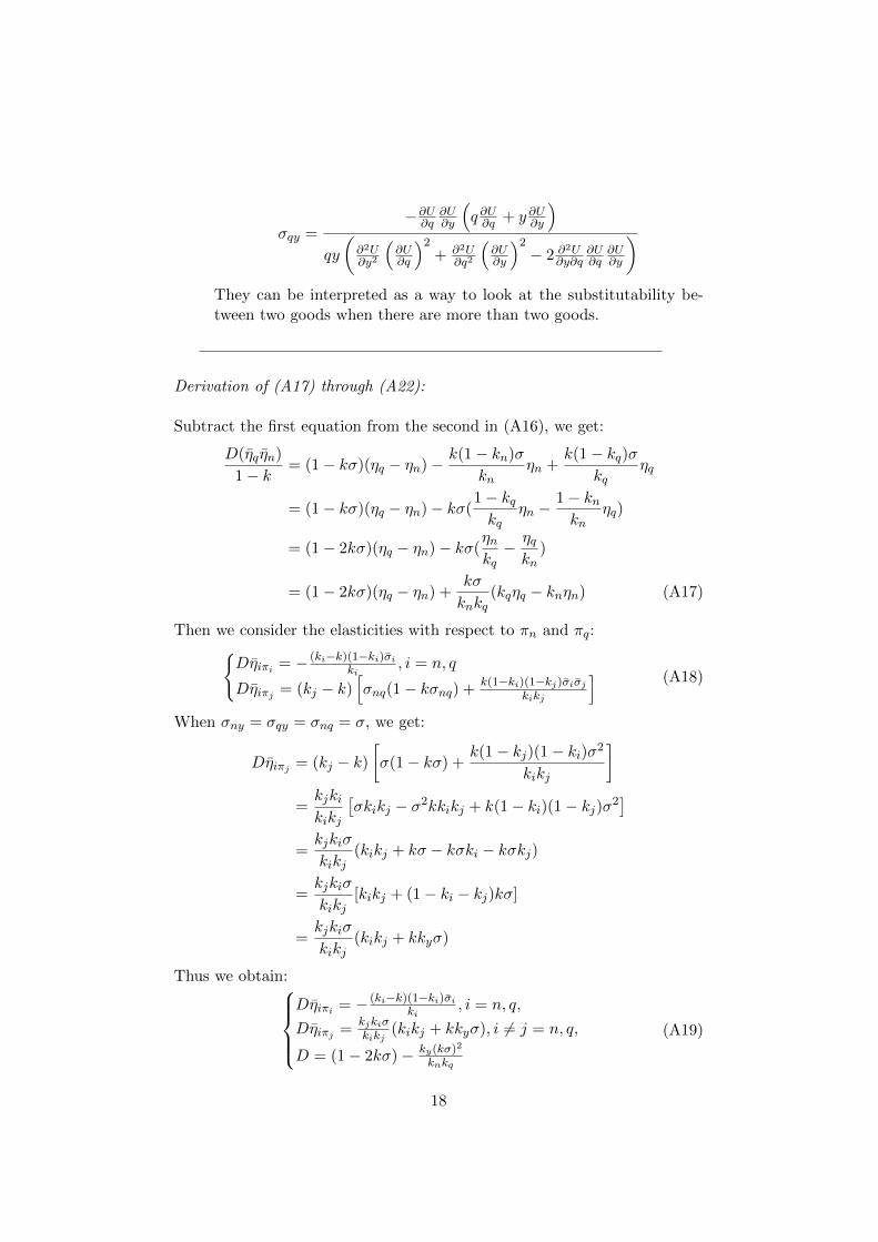
)They can be interpreted as a way to look at the substitutability be-tween two goods when there are more than two goods.

Derivation of (A17) through (A22):

Subtract the first equation from the second in (A16), we get:

D(η̄qη̄n)

1− k= (1− kσ)(ηq − ηn)− k(1− kn)σ

knηn +

k(1− kq)σkq

ηq

= (1− kσ)(ηq − ηn)− kσ(1− kqkq

ηn −1− knkn

ηq)

= (1− 2kσ)(ηq − ηn)− kσ(ηnkq− ηqkn

)

= (1− 2kσ)(ηq − ηn) +kσ

knkq(kqηq − knηn) (A17)

Then we consider the elasticities with respect to πn and πq:{Dη̄iπi = − (ki−k)(1−ki)σ̄i

ki, i = n, q

Dη̄iπj = (kj − k)[σnq(1− kσnq) +

k(1−ki)(1−kj)σ̄iσ̄jkikj

] (A18)

When σny = σqy = σnq = σ, we get:

Dη̄iπj = (kj − k)

[σ(1− kσ) +

k(1− kj)(1− ki)σ2

kikj

]=kjkikikj

[σkikj − σ2kkikj + k(1− ki)(1− kj)σ2

]=kjkiσ

kikj(kikj + kσ − kσki − kσkj)

=kjkiσ

kikj[kikj + (1− ki − kj)kσ]

=kjkiσ

kikj(kikj + kkyσ)

Thus we obtain:Dη̄iπi = − (ki−k)(1−ki)σ̄i

ki, i = n, q,

Dη̄iπj =kjkiσkikj

(kikj + kkyσ), i 6= j = n, q,

D = (1− 2kσ)− ky(kσ)2

knkq

(A19)

18

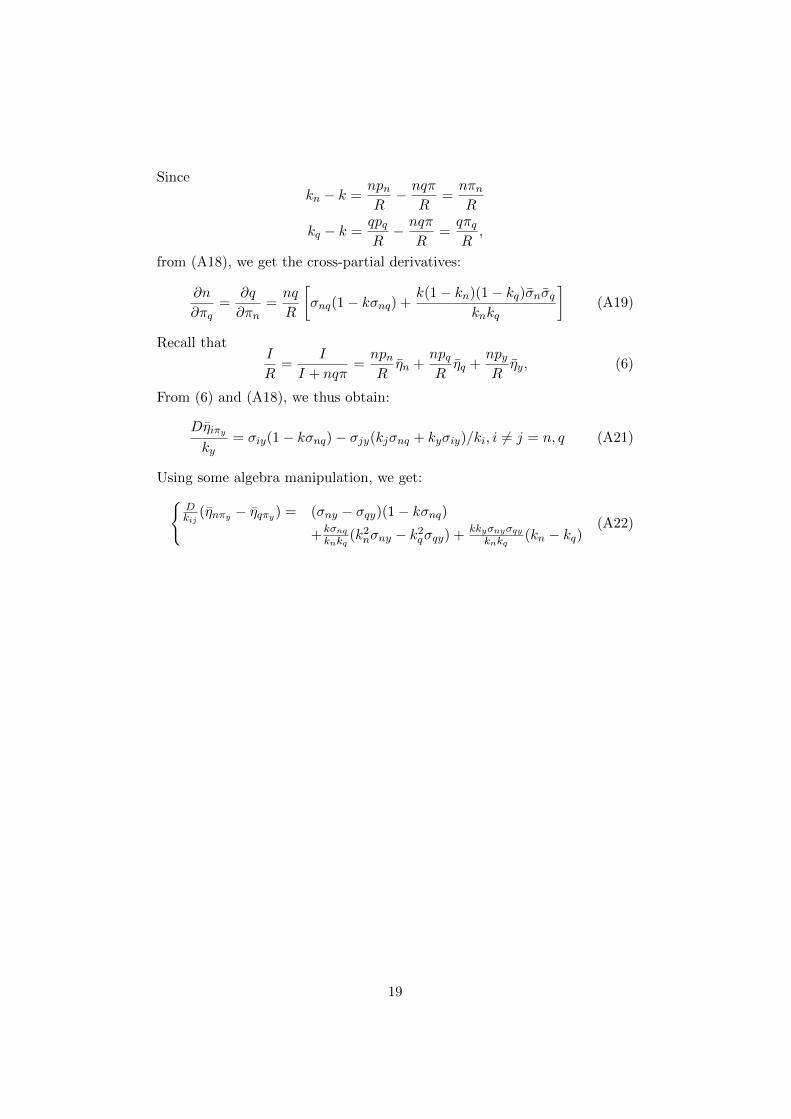
Sincekn − k =

npnR− nqπ

R=nπnR

kq − k =qpqR− nqπ

R=qπqR,

from (A18), we get the cross-partial derivatives:

∂n

∂πq=

∂q

∂πn=nq

R

[σnq(1− kσnq) +

k(1− kn)(1− kq)σ̄nσ̄qknkq

](A19)

Recall thatI

R=

I

I + nqπ=npnR

η̄n +npqRη̄q +

npyRη̄y, (6)

From (6) and (A18), we thus obtain:

Dη̄iπyky

= σiy(1− kσnq)− σjy(kjσnq + kyσiy)/ki, i 6= j = n, q (A21)

Using some algebra manipulation, we get:{Dkij

(η̄nπy − η̄qπy) = (σny − σqy)(1− kσnq)+kσnq

knkq(k2nσny − k2

qσqy) +kkyσnyσqy

knkq(kn − kq)

(A22)

19

References

[1] Dennis N. De Tray, “Child Quality and the Demand for Children”, TheJournal of Political Economy, Vol. 81, No. 2, Part 2: New EconomicApproaches to Fertility (Mar. - Apr., 1973), pp. S70-S95.

[2] Gary S. Becker and H. Gregg Lewiss, “On the Interaction between theQuantity and Quality of Children”, The Journal of Political Economy,Vol. 81, No. 2, Part 2: New Economic Approaches to Fertility (Mar. -Apr., 1973), pp. S279-S288.

[3] Gary S. Becker, “An Economic Analysis of Fertility”, Demographic andEconomic Change in Developed Countries, Princeton: National Bureauof Economic Research, 1960, pp. 209-231.

[4] Gary S. Becker, “A Theory of Social Interactions”, The Journal of Po-litical Economy, Vol. 82, No. 6, Nov. - Dec., 1974, pp. 1063-1093.

[5] H. Thompson, “Substitution Elasticities with Many Inputs”, Appl.Math. Lett. Vol. 10, No. 3, 1997, pp. 123-127.

[6] Theodore W. Schultz, “The Value of Children: An Economic Perspec-tive ”, The Journal of Political Economy, Vol. 81, No. 2, Part 2: NewEconomic Approaches to Fertility (Mar. - Apr., 1973), pp. S2-S13.

[7] Orley Ashenfelter, “Child Quality and the Demand for Children: Com-ment ”, The Journal of Political Economy, Vol. 81, No. 2, Part 2: NewEconomic Approaches to Fertility (Mar. - Apr., 1973), pp. S96-S98.

20

List of Variables

U utilityI full (observed) incomeR total expenditurdn quantity of childrenq quality of childreny other commoditiesλ marginal utility of money incomeπ price of nqπn price of nπq price of qπy price of other commoditiespn shadow price (marginal cost) of npq shadow price (marginal cost) of qpy shadow price (marginal cost) of yMU marginal utilitiesη true elasticitiesη̄ observed elasticitiesσ Allen partial elasticities of substitutionD (1− kσnq)2 − (1− k)2σ̄nσ̄qk nqπ

R

21