notes on cryptography - fenix.tecnico.ulisboa.pt · 9 the rsa cryptographic system 173 ... modern...

Notes on Cryptography

Paulo Mateus, Amılcar Sernadas,

Andre Souto and Luıs Antunes1

2012

1Para se fazer o livro a posteriori

To the guardian

Caution

The themes presented in this work are in a very preliminary phase of maturation. It contains

lots of typos, examples that are not yet complete, definitions that are not written with a unified

notations and theorems that are not properly written. In fact, there are lots of topics still to be

written and others that will deserve a profound reflection before publishing. Many exercises

and examples are part of other books are meant to be used in classes. They will be substituted

in mean time by others that fulfill our purposes of presentations and focus on crucial aspects

that we have in mind.

Reading this lecture notes requires the reader to be prepared to find some problems of compre-

hension and we suggest that it should be complemented with the reading of standard books

used to teach the materials presented here. We suggest for example the readings of [Sti06],

[MVO96], [KL07] and the other references that we put on along the text for a full understanding

of cryptography.

3

Preface

This work is meant to compile in a book the programmatic contents of the introductory course

Criptografia e Protocolos de Seguranca of the Master of Bologne in Mathematics and appli-

cations and also from the Doctoral program me on Security of Information lectured in the

mathematical department of Instituto Superior Tecnico of Universidade Tecnica de Lisboa. It

also uses material lectured in the course Criptografia lectured at computer science department

of Faculdade de Ciencias of Universidade do Porto.

The idea of this work is provide a very useful self contained book about cryptography using

a perspective of a mathematician and also a perspective of a computer scientist in order to be

able to a tool that others can use to teach a similar course.

For financial support the author Andre Souto is deeply thankful to FCT through the grant

SFRH/BPD/76231/2011.

We are grateful to the SQIG members for the nice working ambient and all the encouragement

that they have us.

A special thanks is due to several people with which we had very helpful discussions, feedback

and advising on the themes and the approaches choosen.

2012.

Mathematical Department

5

Instituto Superior Tecnico, Universidade Tecnica de Lisboa

Computer Science Department

Faculdade de Ciencias da Universidade do Porto

Security and Quantum Information Group

Instituto de Telecomunicacoes

Contents

Caution 3

Preface 5

1 Intro 3

I Basic concepts 5

2 Algebraic structures and number theory 9

2.1 Groups, rings and fields . . . . . . . . . . . . . . . . . . . . . . . . . . . . . . . . . 9

2.2 The natural numbers . . . . . . . . . . . . . . . . . . . . . . . . . . . . . . . . . . . 13

2.3 Congruences and modular algebras . . . . . . . . . . . . . . . . . . . . . . . . . . 19

2.3.1 Finite Fields . . . . . . . . . . . . . . . . . . . . . . . . . . . . . . . . . . . . 24

2.4 Exercises . . . . . . . . . . . . . . . . . . . . . . . . . . . . . . . . . . . . . . . . . . 26

3 Probabilities and Shannon entropy 29

3.1 Probability theory . . . . . . . . . . . . . . . . . . . . . . . . . . . . . . . . . . . . . 29

7

3.1.1 The notion of bias of a distribution . . . . . . . . . . . . . . . . . . . . . . . 32

3.2 Entropy and information theory . . . . . . . . . . . . . . . . . . . . . . . . . . . . 34

4 Notion of computational complexity 41

4.1 Pseudo-code as base for computation . . . . . . . . . . . . . . . . . . . . . . . . . 42

4.2 Measuring complexity . . . . . . . . . . . . . . . . . . . . . . . . . . . . . . . . . . 45

4.2.1 The big-Oh notation . . . . . . . . . . . . . . . . . . . . . . . . . . . . . . . 47

4.2.2 Complexity classes . . . . . . . . . . . . . . . . . . . . . . . . . . . . . . . . 50

4.3 One-way functions . . . . . . . . . . . . . . . . . . . . . . . . . . . . . . . . . . . . 56

4.3.1 The candidates to one-way functions . . . . . . . . . . . . . . . . . . . . . 68

II Classical Cryptography 71

5 Classical cryptographic systems 73

5.1 Cryptographic systems . . . . . . . . . . . . . . . . . . . . . . . . . . . . . . . . . . 74

5.1.1 Steganography . . . . . . . . . . . . . . . . . . . . . . . . . . . . . . . . . . 77

5.1.2 The substitution cipher . . . . . . . . . . . . . . . . . . . . . . . . . . . . . 78

5.1.3 The Verman cipher system . . . . . . . . . . . . . . . . . . . . . . . . . . . 82

5.1.4 The Vigenere cipher . . . . . . . . . . . . . . . . . . . . . . . . . . . . . . . 83

5.1.5 The Hill cipher . . . . . . . . . . . . . . . . . . . . . . . . . . . . . . . . . . 85

5.1.6 Stream ciphers . . . . . . . . . . . . . . . . . . . . . . . . . . . . . . . . . . 89

5.1.6.1 Linear Feedback Shift Registers . . . . . . . . . . . . . . . . . . . 90

5.2 Block Cipher Systems . . . . . . . . . . . . . . . . . . . . . . . . . . . . . . . . . . . 92

5.2.1 ECB mode . . . . . . . . . . . . . . . . . . . . . . . . . . . . . . . . . . . . . 93

5.2.2 CBC mode . . . . . . . . . . . . . . . . . . . . . . . . . . . . . . . . . . . . . 94

5.2.3 CFB mode . . . . . . . . . . . . . . . . . . . . . . . . . . . . . . . . . . . . . 96

5.2.4 OFB mode . . . . . . . . . . . . . . . . . . . . . . . . . . . . . . . . . . . . . 99

5.3 Breaking down the cryptographic system . . . . . . . . . . . . . . . . . . . . . . . 101

5.3.1 Breaking down the substitution cipher . . . . . . . . . . . . . . . . . . . . . 106

5.3.2 Breaking the Vigenere cipher . . . . . . . . . . . . . . . . . . . . . . . . . . 110

5.3.3 Breaking the Hill cipher . . . . . . . . . . . . . . . . . . . . . . . . . . . . . 113

5.3.4 Breaking the LFCS . . . . . . . . . . . . . . . . . . . . . . . . . . . . . . . . 115

5.4 Exercises . . . . . . . . . . . . . . . . . . . . . . . . . . . . . . . . . . . . . . . . . . 116

6 Perfect secrecy 121

6.1 Definition of perfect security and results . . . . . . . . . . . . . . . . . . . . . . . . 123

6.2 Exercises . . . . . . . . . . . . . . . . . . . . . . . . . . . . . . . . . . . . . . . . . . 130

7 Block ciphers: DES and AES 133

7.1 Substitution-Permutation Networks . . . . . . . . . . . . . . . . . . . . . . . . . . 134

7.2 DES – Data Encryption Standards . . . . . . . . . . . . . . . . . . . . . . . . . . . . 139

7.2.1 Description of DES . . . . . . . . . . . . . . . . . . . . . . . . . . . . . . . . 140

7.2.2 Breaking down the DES . . . . . . . . . . . . . . . . . . . . . . . . . . . . . 145

7.2.2.1 Linear Approximation of S-boxes . . . . . . . . . . . . . . . . . . 145

7.2.2.2 The differential attack . . . . . . . . . . . . . . . . . . . . . . . . . 150

7.2.2.3 Analytic attack . . . . . . . . . . . . . . . . . . . . . . . . . . . . . 154

7.3 AES – Advanced Encryption Standards . . . . . . . . . . . . . . . . . . . . . . . . 155

7.3.1 Description of AES . . . . . . . . . . . . . . . . . . . . . . . . . . . . . . . . 156

7.4 Exercises . . . . . . . . . . . . . . . . . . . . . . . . . . . . . . . . . . . . . . . . . . 160

III The Public Key Cryptography 163

8 The story behind Public Key Cryptography 165

8.1 Describing a public key cryptographic system . . . . . . . . . . . . . . . . . . . . 168

9 The RSA cryptographic system 173

9.1 The RSA cryptographic system . . . . . . . . . . . . . . . . . . . . . . . . . . . . . 174

9.2 Euclidean Algorithm for the gcd and the modular exponentiation . . . . . . . . . 178

9.3 Checking fast primality of numbers . . . . . . . . . . . . . . . . . . . . . . . . . . 183

9.3.1 The quadratic residue problem and the Legendre and Jacobi symbols . . . 187

9.3.2 Solovay–Strassen algorithm . . . . . . . . . . . . . . . . . . . . . . . . . . . 194

9.3.3 Miller-Rabin’s algorithm for primality test . . . . . . . . . . . . . . . . . . 197

9.3.4 The AKS algorithm proving that Primes ∈ P . . . . . . . . . . . . . . . . 198

9.4 Attacking the RSA - Factorizing n . . . . . . . . . . . . . . . . . . . . . . . . . . . . 206

9.4.1 Pollard’s p− 1 method . . . . . . . . . . . . . . . . . . . . . . . . . . . . . . 207

9.4.2 Dixon’s random square algorithms . . . . . . . . . . . . . . . . . . . . . . . 209

9.4.3 Shor’s algorithm for factorization . . . . . . . . . . . . . . . . . . . . . . . 212

9.4.3.1 quantum mechanics . . . . . . . . . . . . . . . . . . . . . . . . . . 212

9.4.3.2 The algorithm and its explanation . . . . . . . . . . . . . . . . . . 212

9.5 Attacking the RSA - other attacks . . . . . . . . . . . . . . . . . . . . . . . . . . . . 212

9.6 Attacking RSA based on partial information leaked . . . . . . . . . . . . . . . . . 215

9.7 The Rabin’s cryptographic system and its relationship with RSA . . . . . . . . . . 218

9.8 Exercises . . . . . . . . . . . . . . . . . . . . . . . . . . . . . . . . . . . . . . . . . . 227

10 Cryptographic schemes based on the discrete logarithmic problem 235

10.1 The discrete logarithmic problem . . . . . . . . . . . . . . . . . . . . . . . . . . . . 235

10.2 The ElGamal Public-key Cryptographic system . . . . . . . . . . . . . . . . . . . . 237

10.3 Attacking the Discrete Logarithm problem . . . . . . . . . . . . . . . . . . . . . . 240

10.4 The elliptic curves . . . . . . . . . . . . . . . . . . . . . . . . . . . . . . . . . . . . . 247

11 Another approach to factorization - Shor’s quantum algorithms 255

11.1 Notation . . . . . . . . . . . . . . . . . . . . . . . . . . . . . . . . . . . . . . . . . . 257

11.2 The notion of a qubit and its representation . . . . . . . . . . . . . . . . . . . . . . 258

11.2.1 Scoot Aaronson explains the Shor’s algorithm . . . . . . . . . . . . . . . . 261

11.2.2 The Shor’s algorithm for factoring . . . . . . . . . . . . . . . . . . . . . . . 266

11.2.2.1 Quantum Fourier transformation . . . . . . . . . . . . . . . . . . 266

11.2.2.2 The period finding . . . . . . . . . . . . . . . . . . . . . . . . . . . 270

11.2.2.3 Putting together all the ingredients . . . . . . . . . . . . . . . . . 274

11.2.2.4 An example of the Shor’s algorithm for n=15 . . . . . . . . . . . 275

IV Applications of Cryptography 279

12 Digital Signtures 283

12.1 Definition and examples . . . . . . . . . . . . . . . . . . . . . . . . . . . . . . . . . 286

12.2 Secure digital signatures . . . . . . . . . . . . . . . . . . . . . . . . . . . . . . . . . 289

12.3 The ElGamal digital signature scheme . . . . . . . . . . . . . . . . . . . . . . . . . 292

12.4 The notion of hash function . . . . . . . . . . . . . . . . . . . . . . . . . . . . . . . 295

13 Zero knowledge 299

13.1 Undeniable signatures . . . . . . . . . . . . . . . . . . . . . . . . . . . . . . . . . . 308

14 Stuff 317

V Bibliography 319

Bibliography 321

CHAPTER 1

Intro

To be done later...

“Cryptography is the art of writing codes and solving codes...”

Need to say that the material collected in this work is original and was influenced by many

excellent books containing their own perspective of Cryptography. We were influenced mainly

by the following references: [Sti06], [KL07], [HPS08], [MVO96],

3

Part I

Basic concepts

5

In this part it is presented some basic concepts and constructions that will crucial and widely

used in due course on the presentation of the themes of these notes and are fundamental in

modern cryptography has they are they are their cornerstones.

It is presented, in the next Chapter and, in particular, in Section2.1, the material related with

algebra. In Section 2.2 it is presented the foundation of number theory and in Section 2.3

its is presented some notions concerning modular algebras. In Chapter 3 is presented the

topics about Information theory and in particular, in Section 3.1 it is introduced the theory

of probabilities and in Section 3.2 it is presented the concept and basic results related with

Shannon entropy.

7

CH

AP

TE

R2

CHAPTER 2

Algebraic structures and number theory

This chapter begins by presenting the common algebraic structures that will be consider in

these notes, namely, groups, rings and fields. They are important for the subsequent sections

where the basic notions of number theory and modular algebras is introduced. It is suggested

the reading of the book [Lan02] of Lang to the interested reader for a complete study on algebra

topics.

• • • • • • • • • • • • • • • • • • • • • • • • • • • • • • • • • • • • •

SECTION 2.1

Groups, rings and fields

Cryptography is all about processes of transforming messages into another messages among a

finite space of possible messages. Thus, the set of messages have certain algebraic structures in

order to be closed under the transformation operations.

In this section it is surveyed some of the basic algebraic structures, namely groups, rings

and fields, that are central concepts of abstract algebra, and are also basic tools for modern

cryptography.

Roughly speaking, a group is a set of objects with an operation defined between any two objects

in the set with certain properties, a ring is a set with two operations that is a group for the

9

CH

AP

TE

R2

2.1 Groups, rings and fields

first operation and the second operation is distributive with respect to the group operation.

Finally, a field is commutative ring with unity in which every non null element has inverse

(with respect to the second operation).

Definition 2.1.1 (Monoid)

Let G be a nonempty set and : G × G → G and binary operator in G. The pair (G, ) is

called a monoid if and only if the following properties hold:

Identity: There is e ∈ G such that for all a ∈ G, a e = a.

Associativity: For all a, b, c ∈ G, a (b c) = (a b) c.

Examples of monoinds are (N,+), (N, ·), (Z,+), (Z, ·), (Q,+), (Q, ·), (R,+), (R, ·), (C,+)

and (C, ·), where + and · are the usual sum and product operations in those sets.

Definition 2.1.2 (Group)

Let (G, ) be a monoid. The monoid is called a group if and only if every a ∈ G has inverse,

i.e, there is an element b ∈ G such that a b = e.

A group (G, ) is commutative or Abelian if in addition, one has, for all a, b ∈ G, a b =

b a.

Examples of groups are (N,+), (Z,+). Another important example of groups are (N∗, ·),

(Z∗, ·), (Q∗, ·), (R∗, ·), where C∗ = C− 0.

Example 2.1.1. Let n be a natural number and let Zn be the set of all possibles remainders by n, i.e.,

Zn = 0, · · · , n− 1

and given a, b ∈ Zn define a + b as the remainder of a + b by n. Then (Zn,+) is an example of a finite

group, i.e., a group over a finite set. This particular type of groups will be discussed in more detail later

on (in Section 2.3) and will widely used.

Definition 2.1.3 (Subgroup)

A subgroup of a group (G, ) is a non-empty subset H of G which is itself a group under

the same operation .

Clearly (N,+) is a subgroup of (Z,+). Also (e, ) is a subgroup of (G, ).

10

CH

AP

TE

R2

Chapter 2. Algebraic structures and number theory

Definition 2.1.4

Let (G, ) be a finite group. The number of elements in G is called the order of G and is

denoted by ord(G).

Theorem 2.1.1 (Lagrange)

Let G be a finite group. If H is a subgroup of G then ord(H) divides ord(G).

Proof: To prove this theorem first consider the sets:

aH = a b : b ∈ G.

usually called lateral classes of H.

Claim 2.1.2. aH = bH if and only if a b−1 ∈ H.

Proof:

(⇒) Since a ∈ aH = bH there exists h ∈ H such that a = b h. Thus, b−1 a = b−1 (b h) =

(b−1 b) h = e h = h. Hence b−1 a ∈ H.

(⇐) Since b−1 a ∈ H then there exists h ∈ H such that b−1 a = h⇔ a = b h, hence a ∈ bH.

Thus if g ∈ aH then g = a h′ for some h′ ∈ H, hence g = b h h′ = b h′′ Since H is a

subgroup h′′ ∈ H and therefore g ∈ bH, which means that aH ⊂ bH. The other inclusion is

obtained observing that, since b−1 a = h then b = a h−1.

Claim 2.1.3. If aH ∩ bH 6= ∅ then aH = bH.

Proof: If aH ∩ bH 6= ∅ then there exists g ∈ G such that g = a h = b h′, hence b−1 a =

h′ h−1. Since h′ h−1 ∈ H then by the previous item aH = bH.

Claim 2.1.4. For all a ∈ G, #aH = #H.

Proof: It is enough to prove that for all a ∈ G, fa : H → aH defined by fa(h) = a h is a

bijection. It is clear from the definition of ah that fa is surjective. To prove that fa is injective

notice that if a h = a h′ then a−1 a h = h′ i.e., h = h′.

Claim 2.1.5. All the different lateral classes of H form a partition of G.

11

CH

AP

TE

R2

2.1 Groups, rings and fields

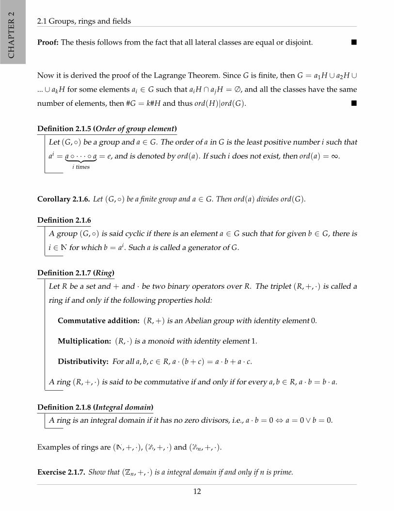
Proof: The thesis follows from the fact that all lateral classes are equal or disjoint.

Now it is derived the proof of the Lagrange Theorem. Since G is finite, then G = a1H ∪ a2H ∪

... ∪ akH for some elements ai ∈ G such that aiH ∩ ajH = ∅, and all the classes have the same

number of elements, then #G = k#H and thus ord(H)|ord(G).

Definition 2.1.5 (Order of group element)

Let (G, ) be a group and a ∈ G. The order of a in G is the least positive number i such that

ai = a · · · a︸︷︷︸i times

= e, and is denoted by ord(a). If such i does not exist, then ord(a) = ∞.

Corollary 2.1.6. Let (G, ) be a finite group and a ∈ G. Then ord(a) divides ord(G).

Definition 2.1.6

A group (G, ) is said cyclic if there is an element a ∈ G such that for given b ∈ G, there is

i ∈ N for which b = ai. Such a is called a generator of G.

Definition 2.1.7 (Ring)

Let R be a set and + and · be two binary operators over R. The triplet (R,+, ·) is called a

ring if and only if the following properties hold:

Commutative addition: (R,+) is an Abelian group with identity element 0.

Multiplication: (R, ·) is a monoid with identity element 1.

Distributivity: For all a, b, c ∈ R, a · (b + c) = a · b + a · c.

A ring (R,+, ·) is said to be commutative if and only if for every a, b ∈ R, a · b = b · a.

Definition 2.1.8 (Integral domain)

A ring is an integral domain if it has no zero divisors, i.e., a · b = 0⇔ a = 0∨ b = 0.

Examples of rings are (N,+, ·), (Z,+, ·) and (Zn,+, ·).

Exercise 2.1.7. Show that (Zn,+, ·) is a integral domain if and only if n is prime.

12

CH

AP

TE

R2


Definition 2.1.9 (Field)

A tuple (F,+, ·) is said to be a field if and only if the following properties hold:

1. (F,+, ·) is an integral domain.

2. (F− 0, ·) is an Abelian group.

• • • • • • • • • • • • • • • • • • • • • • • • • • • • • • • • • • • • •

SECTION 2.2

The natural numbers

For further readings on this topic it is suggested to the reader the book [And71] of G. Andrews

and the book [IR90] of K. Ireland and M. Rosen.

As usual the natural numbers are represented by N and the integers by Z.

One of the centrals in Number Theory and, in particular, in Cryptography is the concept of

divisibility.

Theorem 2.2.1 (Euclidean decomposition)

Let a and b be two arbitrary integers. If a 6= 0 then there are integers d and r, called

respectively quotient e remainder, such thatb = a · d + r

0 ≤ r < |a|.

Such d and r are unique.

Proof: First, it is shown the existence of such integers.

If |b| < |a| then b = a · 0 + b and thus, in this case just take d = 0 and r = b. Assume that

|b| ≥ |a|. Since Z is a well ordered set, and thus, in particular, each of its nonempty subsets

have first element, it follows that the set

n ∈ Z : b < a · n

13

CH

AP

TE

R2

2.2 The natural numbers

has a minimum element. Let n be that minimum. Take d = n− 1, i.e., the largest integers such

that a · d does not exceed b. By construction d ∈ Z.

On the other hand, taking r = b− a · d one also has that r ∈ N and a · d+ r = a · d+ b− a · d = b.

To finish the proof of the existence in remains to prove that r ≤ a. If r was larger than |a| this

would mean that |b| − |a · d| > |a| which would be equivalent to say that |b| > |a| · |d + 1|,

contradicting the choice of d.

To prove the uniqueness of d and r assume, by reduction to absurd, that there are d′ 6= d e

r′ 6= r such that b = a · d′ + r′ and 0 ≤ r′ < |a|. Then, one would have that a · d + r = a · d′ + r′,

i.e., a · (d− d′) = r′ − r and |r− r′| < |a|. Hence, since d 6= d′, |d− d′| is at least 1, one would

get that |a| ≤ |a| · |d′ − d| = |r− r′| < |a| which is absurd. Thus d′ = d and r = r′.

Given two integers a and b, one says that b divides a, or that b is a multiple of a, or yet that b

is a divisor of a, and it is usually written by b|a is in the decomposition described in the last

theorem r = 0, i.e., if there are integers d (necessarily unique) such that a = b · d. In the next

proposition some of the basic properties of the divisibility relation are stated.

Proposition 2.2.1. Let a, b, c, d, e ∈ Z. The relation ·|· has the following properties:

1. it is reflexive, i.e., a|a;

2. if a|b then a ≤ b;

3. it is transitive, i.e., if b|a and c|b then c|a;

4. it is antisymmetric, i.e., if b|a and a|b then a = b;

5. if a|b e a|c then a|(b · d± c · e);

6. if a 6 |b · c then a 6 |b and a 6 |c;

7. if a|b e a 6 |(b · d + c) then a 6 |c.

The proof of these properties is left to the interested reader.

14

CH

AP

TE

R2


Definition 2.2.1

Let a and b integers. The natural number d is said the grater common divisor between a

and b, if: d|a ∧ d|b

∀c (c|a ∧ c|b =⇒ c|d).

It is usual to denote by gdc(a, b) the grater common divisor between a and b. It is also

common, in particular, if gcd(a, b) = 1 then a and b are said to be co-prime or relatively

prime.

Notice that the great common divisor is unique since if d and d′ were such that d = gcd(a, b)

and d′ = gcd(a, b), then, in particular, one would have that d|d′ and d′|d, whence by the last

properties one would have d = d′.

Exercise 2.2.2. Let a, b and c be non null integers. Show that if a|bc and a and b are co-primes, then

a|c.

Theorem 2.2.2

Let a and b be non null integers. Then

gcd(a, b) = min z : z > 0 ∧ ∃ x, y ∈ Z (z = a · x + b · y) .

Proof: Consider the set C = z : z > 0 ∧ ∃ x, y ∈ N (z = a · x + b · y). Notice that C 6= ∅,

since a and b being non null, z = a2 + b2 = a . a + b . b belongs to C. Thus, since Z is well

ordered, C has a first element.

Let d be the first element and let x, y ∈ Z such that d = a · x + b · y and 0 ≤ y < |a|.

To show that d|a assume that q and r are such that a = d . q + r e 0 ≤ r ≤ |d| as stated in

Theorem 2.2.1. Hence r = a − d . q = a − (a · x + b · y) . q = a . (1− q . x) + b(−yq) and thus

r ∈ C. Thus, if r > 0 then, in particular on would have that r would be at least the minimum

of C, i.e., r ≥ d, which is not possible. It follows that r = 0 and thus d|a. In an analogous way

one can show that d|b.

With this reasoning one showed that d is a common divisor of a and b. Assume that c is another

common divisor of a and b. Hence, in particular c divides a · x and b · y and, hence, by previous

15

CH

AP

TE

R2


proposition c|(a · x + b · y), i.e c|d, which implies that d is the greater common divisor.

As an example consider the gcd(12, 20) = 4. In fact one can write 4 as the following combina-

tion of 12 and 20: 4 = 2 . 12− 1 . 20.

The next exercise asks the reader to prove some of basic properties of the greater common

divisor.

Exercise 2.2.3. Let a, b, c and d be non null integers. Show that:

1. 1 = gcd(a, b) if and only if there are x, y ∈ N such that 1 = a . x + b . y;

2. gcd(

agcd(a, b)

,b

gcd(a, b)

)= 1;

3. gcd(a . d, b . d) = d · gcd(a, b);

4. if a|b . c thena

gcd(a, b)

∣∣∣∣ c.

Definition 2.2.2

An number p ∈ N is called prime if p > 1 and its unique divisors are 1 and p.

A number n ∈ N that is not prime, i.e., a number that has at least one non trivial divisor (i.e.,

different from 1 and itself) is called composed.

It is widely known any composed natural number n can be written as a product of prime

numbers.

Theorem 2.2.3 (Fundamental of arithmetic)

let n be a natural number such that n > 1. Then there are prime numbers p1 < · · · < pk and

naturals a1, · · · , ak such that n = ∏ paii .

Proof:[Sketch of the proof] If n is already a prime the result is trivially true. Assume without

loss of generality that n is not prime, i.e., there are m ∈ N such that m > 1 and m|n. Consider

the set

D1 = m : m|n ∧m > 1

of natural divisors of n. Since D1 is a subset of N it admits minimum element, say p.

16

CH

AP

TE

R2


Claim 2.2.4. p is a prime number.

In fact, if p was not prime then itself would admit a nontrivial divisor q < p and thus, since

p|n and q|p then by Proposition 2.2.1 one would have q|n, contradicting the choice of q.

Take p1 = p and consider now the set

D2 =

m : m

∣∣∣∣ np1∧m > 1

.

Again the minimum of D2 is a prime number p. Take p2 = p and repeat the process consider-

ing, while possible, the set:

Di =

m : m

∣∣∣∣∣ n∏j pj<i

∧m > 1

.

Notice that this process must finish. It is easy to see that with at most n/2 steps the set Di will

be empty since each time one considers a new subset of divisors the upper bound of the set is

divided by two (the least prime number candidate to be in D).

Notice also that, by construction, pi ≤ pi+1. Hence the thesis follows by associating the similar

primes.

Theorem 2.2.4

The set of prime numbers is infinite and the difference between two consecutive prime

numbers can be arbitrarily large.

Proof: Assume by contradiction that the set of prime numbers is finite, i.e., that the set of prime

numbers is:

P = p1, · · · , pk.

Let n = p1 . · · · . pk + 1. Notice that n is larger than any number in P since it is the product of all

of elements of P which are prime numbers and thus, in particular, larger than 1. Thus n is not a

prime and thus must be compose. Thus, it must to exist pi ∈ P such that pi|n. Consequently by

Proposition 2.2.1, since pi|p1 . · · · . pk one would conclude that pi|n− p1 . · · · . pk which would

imply that pi|1 and thus pi = 1 contradicting the primality of pi. The contradiction followed

from the supposition that P was finite.

17

CH

AP

TE

R2


To show that the difference between two consecutive prime numbers can be arbitrarily large it

is enough to observe that the sequence of the form ai = (n + 1)! + i with 2 ≤ i ≤ n + 1 does

not contain any prime number. In fact, for all i such that 2 ≤ i ≤ n + 1, i|(n + 1)! and, thus,

again by Proposition 2.2.1, i|(n + 1)! + i. Notice that the sequence ai can be arbitrarily large.

The last proposition establishes the existence of infinitely many prime numbers but it does not

say states anything about its density, as a subset of N. The next theorem gives an idea of the

prime numbers are distributed giving an asymptotic behavior.

Theorem 2.2.5 (Prime numbers theorem)

Let π(n) be the number of primes between 2 and n. Thus:

π(n) = limn

nln n

where ln is used to denote, as usual, the logarithm computed in the natural base e.

Proof: to be done

For any positive integer n define φ(n), the Euler function1 as the number of positive integers a

less than n such that a is relatively prime to n. By definition of prime number it is easy to see

that φ(p) = p− 1. Also, φ(pn) = pn − pn−1, since among the pn − 1 positive integers less than

pn there are pn−1 − 1 numbers that are not co-prime to pn.

Exercise 2.2.5. Show that if m and n are co-primes then φ(m · n) = φ(m) · φ(n) and conclude that, in

particular, if m and n are different prime numbers, φ(m · n) = (m− 1)(n− 1).

Exercise 2.2.6. Show that if n is a non null natural number, then ∑d|n

φ(d).

1By a function f from A to B, written f : A → B, we mean that dom f = A and the img f ⊆ B since we only

work in this course with total functions.

18

CH

AP

TE

R2


• • • • • • • • • • • • • • • • • • • • • • • • • • • • • • • • • • • • •

SECTION 2.3

Congruences and modular algebras

In this section it is studied the theme of congruences modulo a natural number and it is

explored some of its basic properties that well be used in due course in the subsequent chapters

of this work.

Definition 2.3.1 (congruence modulo n)

Let a, b be integers and n a natural number non null. It is said that a is congruent with

b modulo n, or that a and b are congruents modulo n, and one writes a ≡ b (mod n), if

n|b− a.

In the previous definition one may have n = 1, but this case is not very interesting from the

mathematical properties point of view since any two integers are divisible by 1 and thus no

useful properties can be explored. The following theorem gives an equivalent formulation that

is commonly used.

Theorem 2.3.1

Let a, b be integers and n a non null natural number. a and b are congruents modulo n if

and only if the remainder of the quotient of each of them by n are equal.

Proof:

(←)

Let d1, d2, r1 and r2 be integers such that a = d1 . n + r1, b = d2 . n + r2 and 0 < r1, r2 <

n. Since a ≡ b (mod n), on has n|(b − a) and thus n|(d1 . n + r1 − d2 . n − r2). Hence, by

Proposition 2.2.1 one can conclude that n|(r1 − r2). Since 0 < r1, r2 < n then r1 = r2, as

envisaged.

(→)

Assume that a = d1 . n + r and that b = d2 . n + r with 0 < r < n, for some integers d1, d2 and

r. Hence a− b = (d1 − d2) . n and, so, n|a− b, i.e., a ≡ b (mod n).

19

CH

AP

TE

R2

2.3 Congruences and modular algebras

Theorem 2.3.2

The congruence modulo a natural number relationship ≡ is an equivalence relationship in

Z, i.e., given a, b, c ∈ Z and n ∈ N non null:

• ≡ is reflexive: a ≡ a (mod n);

• ≡ is symmetric: if a ≡ b (mod n) then b ≡ a (mod n);

• ≡ is transitive: if a ≡ b (mod n) and b ≡ c (mod n) then a ≡ c (mod n);

Proof: To prove the reflexivity just observe that n|a− a = 0.

For the symmetry notice that if n|b− a then n|a− b = −(b− a).

To show the transitivity notice that if n|b− a and n|c− b then n|c− a = (c− b) + (b− a).

In the next exercise the reader is invited to show some of the basic properties of the congru-

ences.

Exercise 2.3.1. Let a, b, c and d be integers and n > 1. Show that:

1. If a ≡ b (mod n) and c ≡ d (mod n) then a + c ≡ b + d (mod n);

2. If a ≡ b (mod n) then −a ≡ −b (mod n);

3. If a ≡ b (mod n) and c ≡ d (mod n) then a · c ≡ b · d (mod n). In particular, for all d, if

a ≡ b (mod n) then ad ≡ bd (mod n);

4. a + b ≡ b + a (mod n);

5. (a + b) + c ≡ a + (b + c) ≡ a + b + c (mod n);

6. (a + b) · c ≡ c · (a + b) ≡ a · c + b · c (mod n).

It is well known that an equivalence relationship like congruence modulo n over a set partitions

Z into equivalence classes. Since there are at most n possible different remainders considering

the quotient by n, Z is portioned into n classes each of them containing exactly the numbers

that are congruent modulo n. Denoting by a the class of equivalence of a (mod n), i.e.,

a = x ∈ Z : a ≡ x (mod n) = aZ

20

CH

AP

TE

R2


then one can consider the quotient set Zn = Z/ ≡n formed by the equivalent classes modulo n

i.e.,

Zn =

0, 1, · · · , n− 1

.

Using the properties established in Exercise 2.3.1 it is easy to define + and × as follows:

• a + b = a + b

• a× b = a · b

It is also easy to derive the following theorem:

Theorem 2.3.3

(Zn,+) is a group.

Exercise 2.3.2. Show or refute the following statement. “For all n ∈ N, (Zn,×) is a group.”

Clearly the statement of the last exercise is false since for example, when n = p× q where p and

q are primes, then p does not have a symmetric element, i.e., the equation p× x ≡ 1 (mod n)

does not have any solution. In fact, in general, the equation “ax ≡ b (mod n)” is solvable if

and only if gcd(a, n)|b.

Exercise 2.3.3. Show that for a and b integers and n > 1, the equation ax ≡ b (mod n) is solvable if

and only if gcd(a, n)|b.

It follows from the previous exercise that (Z∗n,×), where Z∗n = a : gdc(a, n) = 1 is also a

group. In fact, using the properties established in Exercise 2.3.1 one can derive the following

theorem.

Proposition 2.3.4. If n is prime, (Z∗n,+,×) is a ring with the property that (Z∗n,+) is a cyclic group.

The Chinese remainder theorem is very useful tool that will be used in due course and states

that if m1, m2, . . . , mr are natural numbers greater than or equal to 2 that are pairwise co-primes,

and if 0 ≤ ai < mi for 1 ≤ i ≤ r, then there is a unique integer a such that 0 ≤ a < m =

m1m2 · · ·mr and a ≡ ai (mod m)1 for 1 ≤ i ≤ r.

21

CH

AP

TE

R2


Theorem 2.3.4 (Chinese remainder theorem)

Let m1, m2, . . . , mr be positive integers that are pairwise co-primes. Let a1, a2, . . . , ar be

arbitrary integers. Then there is an integer a such that

a ≡ a1 (mod m1)

a ≡ a2 (mod m2)

...

a ≡ ar (mod mr)

.

Furthermore, a is unique modulo M = m1 ×m2 × · · ·mr.

Proof: The proof is carried out by finding an algorithm for constructing a. For each 1 ≤ i ≤ r,

define Mi by

Mi = (M/mi)φ(mi).

Since M/mi is relatively prime to mi and divisible by mj for every j not equal to i, one has that

Mi ≡ 1 (mod mi)

Mj ≡ 0 (mod mi) if j 6= i.

Also consider a as

a = a1 ×M1 + a2 ×M2 + · · ·+ ar ×Mr.

To see that a is unique modulo M, let b be any other integer satisfying all the congruences.

Then for each mi, a and b are congruent modulo mi. In other words, mi divides b− a. Since this

is true for every i, M divides b− a which means that

a ≡ b (mod M).

Theorem 2.3.5 (Fermat’s little theorem)

Let p and a be two natural numbers. If p is prime and p 6 |a, then ap−1 ≡ 1 (mod p).

From the fact that p is prime and for that reason φ(p) = p − 1, Fermat’s little theorem is a

special case of the following theorem.

22

CH

AP

TE

R2


Theorem 2.3.6 (Euler’s theorem)

Let n and a be two natural numbers. If gcd(a, n) = 1 then aφ(n) ≡ 1 (mod n).

Proof: Since gcd(a, n) = 1 then a (mod n) ∈ Z∗n. Thus, by Theorem 2.1.6 ord(a)|ord(Z∗n) ⇔

ord(a)|φ(n), which implies that, there is d ∈ N such that φ(n) = d · ord(a). On the other hand,

by definition of ord(a) in Zn, aord(a) ≡ 1 (mod n). So by Exercise 2.3.1.3

1 ≡ 1d ≡ (aord(a))d ≡ aφ(n) (mod n).

Theorem 2.3.7

Let p and a be two natural numbers. If p is prime then ap ≡ a (mod p).

The proof of this theorem is left to the interested reader.

Theorem 2.3.8

Let p and a be two natural numbers such that p is prime. Then a is a generator of Z∗p if and

only if a(p−1)/q 6≡ 1 (mod p) for all primes q such that q|(p− 1).

Proof:

(←)

If a is a generator of Zp∗ then, for all 1 ≤ i ≤ p− 2, ai 6≡ 1 (mod p) and thus, in particular, the

result follows.

(→)

Assume that a is not a generator of Z∗p. Let d be the order of a, i.e., ad ≡ 1 (mod p). Then,

d < p− 1 and by Lagrange’s Theorem 2.1.1, one has d|(p− 1). Hence (p− 1)/d is an integer

exceeding 1. Let q be a prime divisor of (p− 1)/d. Clearly, d|((p− 1)/q). Since ad ≡ 1 (mod p)

and d|((p− 1)/q), it follows that a(p−1)/q ≡ adc(mod p) ≡ 1 (mod p).

23

CH

AP

TE

R2


• • •

2.3.1 Finite Fields

In this sub subsection it is discussed other kind of finite fields other done Z∗p for p is prime. In

particular it will be discuss field with q = pn elements where p is prime and n >1 is an integer.

Definition 2.3.2

Let p be a prime number. The set Zp[x] is the set of all polynomials with coefficients over

Zp. With the usual operations of sum and multiplication over Zp then (Zp[x],+,×) is a

finite ring.

Definition 2.3.3

Let (Zp[x],+,×) be a finite ring and let f (x), g(x) be two polynomials in Zp[x]. One says

that f (x) divides g(x) and denotes it by f (x)|g(x) if there exists q(x) ∈ Zp[x] such that

g(x) = q(x)× f (x).

Definition 2.3.4

Let (Zp[x],+,×) be a finite ring and let f (x) be a polynomial in Zp[x]. One says that f has

degree n, and denotes by deg( f ) = n, if the term axn is the highest non null term.

Definition 2.3.5

Let (Zp[x],+,×) be a finite ring and let f (x), g(x), h(x) be polynomials in Zp[x]. Assume

that deg( f ) > 1. Then one defines g(x) ≡ h(x) (mod f (x)) if f (x)|(g(x)− h(x)).

Let now Zp[x] be a ring and let f (x) be a polynomial in Zp[x] of degree at least 1. The

ring of polynomials “modulo f (x)”, denoted by Zp[x]/( f (x)) is obtained by considering all

possible remainders modulo f (x). Notice that, again by the Euclides algorithm, given g(x)

there are unique polynomials q(x) (the quotient) and r(x) (the remainder) such that g(x) =

q(x) f (x) + r(x) and deg(r) < n, and hence any polynomial in Zp[x] is congruent modulo f (x)

to a polynomial of degree n− 1, which implies that Zp[x]/( f (x)) is the set of all pn polynomial

of degree at most n− 1.

24

CH

AP

TE

R2


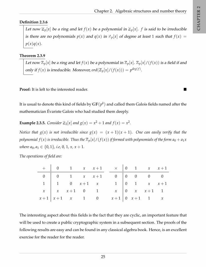
Definition 2.3.6

Let now Zp[x] be a ring and let f (x) be a polynomial in Zp[x]. f is said to be irreducible

is there are no polynomials p(x) and q(x) in Zp[x] of degree at least 1 such that f (x) =

p(x)q(x).

Theorem 2.3.9

Let now Zp[x] be a ring and let f (x) be a polynomial in Zp[x]. Zp[x]/( f (x)) is a field if and

only if f (x) is irreducible. Moreover, ord(Zp[x]/( f (x))) = pdeg( f ).

Proof: It is left to the interested reader.

It is usual to denote this kind of fields by GF(pk) and called them Galois fields named after the

mathematician Evariste Galois who had studied them deeply.

Example 2.3.5. Consider Z2[x] and g(x) = x2 + 1 and f (x) = x2.

Notice that g(x) is not irreducible since g(x) = (x + 1)(x + 1). One can easily verify that the

polynomial f (x) is irreducible. Thus the Zp[x]/( f (x)) if formed with polynomials of the form a0 + a1x

where a0, a1 ∈ 0, 1, i.e, 0, 1, x, x + 1.

The operations of field are:

+ 0 1 x x + 1

0 0 1 x x + 1

1 1 0 x + 1 x

x x x + 1 0 1

x + 1 x + 1 x 1 0

× 0 1 x x + 1

0 0 0 0 0

1 0 1 x x + 1

x 0 x x + 1 1

x + 1 0 x + 1 1 x

The interesting aspect about this fields is the fact that they are cyclic, an important feature that

will be used to create a public cryptographic system in a subsequent section. The proofs of the

following results are easy and can be found in any classical algebra book. Hence, is an excellent

exercise for the reader for the reader.

25

CH

AP

TE

R2

2.4 Exercises

Theorem 2.3.10

Let Zp[x] be a ring and k an integer. There exists an irreducible polynomial f (x) of degree

k in Zp[x]. Moreover, if h(x) is another irreducible polynomial of degree k in Zp[x] then

Zp[x]/( f (x)) and Zp[x]/(h(x)) are isomorphic.

Theorem 2.3.11

Let Zp[x] be a ring and f (x) an irreducible polynomial in Zp[x]. Then Zp[x]/( f (x)) is cyclic.

• • • • • • • • • • • • • • • • • • • • • • • • • • • • • • • • • • • • •

SECTION 2.4

Exercises

Exercise 2.4.1. Assume that G be a finite group, and let g be an element of G of order a. Show that

gn = gm if and only if n ≡ m (mod a).

Exercise 2.4.2. Show that if xn−1 ≡ 1 (mod n) for all integers x that are not multiples of n, then n is

prime.

Notice that a slightly weaker statement that xn−1 ≡ 1 (mod n) for all x such that gcd(x, n) = 1

is not enough not imply that n is prime. There are numbers, called Carmichael numbers that

are counterexamples for this statement.

Exercise 2.4.3. Let p be prime number. Show that (p− 1)! ≡ −1 (mod p).

This exercise is known as Wilson’s Theorem.

The next exercise will be important for the understanding the work of public key cryptographic

systems.

Exercise 2.4.4. Find the least non-negative residue of 315 (mod 1)7 and 1581 (mod 1)3, without

carrying long multiplications.

Exercise 2.4.5. Use Fermat’s theorem 2.3.5 to compute 347 (mod 2)3.

The next exercise intends to provide the reader a mechanism to compute the inverses modulo

n.

26

CH

AP

TE

R2


Exercise 2.4.6. Using the Euclides algorithm for division, compute the inverses of:

1. 2 in Z11;

2. 7 in Z15;

3. 7 in Z16;

4. 5 in Z13;

Exercise 2.4.7. Use the Lagrange theorem 2.1.1 to determine the inverses of the previous exercise.

Exercise 2.4.8. Compute all the solutions with 0 ≤ x ≤ 34 of the following system of equationsx ≡ 4 (mod 5)

x ≡ 5 (mod 7)

Exercise 2.4.9. Compute all the solutions with 0 ≤ x ≤ 104 of the following system of equationsx ≡ 2 (mod 3)

x ≡ 4 (mod 5)

x ≡ 5 (mod 7)

Exercise 2.4.10. Show that every irreducible polynomial in Zp[x] is a divisor of xpn − x for some n.

Exercise 2.4.11. Construct a finite field with 8 elements. hint: find an irreducible polynomial of degree

3 in Z2.

Exercise 2.4.12. Show thatab = ac, with a 6= 0, does not necessarily imply b = c in a ring. Envisaged

the validity of this statement in a ?eld?

Exercise 2.4.13. Show that Z/Zn is a ?eld if and only if n is a prime number.

27

CH

AP

TE

R2

2.4 Exercises

28

CH

AP

TE

R3

CH

AP

TE

R3

CHAPTER 3

Probabilities and Shannon entropy

In this chapter is introduced all the concepts regarding probabilities that will be used in due

course on these notes. It is a central topic one talks about cryptography and this relation will

become clear later on the text. Related with probabilities and cryptography is also the concept

of Shannon entropy that is presented in Section 3.2.

• • • • • • • • • • • • • • • • • • • • • • • • • • • • • • • • • • • • •

SECTION 3.1

Probability theory

The reader is referred, for example, to the book [Kal02] for further and details development on

this issue. Here it is presented the necessary concepts and main results for the understanding

of the rest of the material presented in this book.

The word probability, in mathematics, is used to refer a measure of the weight of empirical

evidence that an event will occur among several ones.

Let X be an experiment that can produce several possible results. The collection of all results is

called the sample space of the experiment. One possible collection of allowed results is called

an event. For example, rolling a die can produce six possible results and the subset 1, 3, 5 is

an event that corresponds to “obtaining an odd number on the die”.

29

CH

AP

TE

R3

CH

AP

TE

R3

3.1 Probability theory

A probability is an assignment of a value between zero and one to every event, with the

requirement that the event made up of all possible results (in the example of the die, the event

1, 2, 3, 4, 5, 6) is assigned with the value one. The function that assigns to every elementary

event a probability is called a Probability distribution over the power set of possible results.

Definition 3.1.1

A discrete random variable X is a finite set X together with a probability distribution de-

fined on X. The probability that the random variable X takes on the value x is denoted by

Pr[X = x] or by Pr[x] if the random variable X is clear from the context. It must be the case

that the three following conditions are satisfied:

Pr(X = x) ≥ 0, ∀x ∈ X;

Pr(X) = 1;

Pr(X ∈ A ∪ B) = Pr(X ∈ A) + Pr(X ∈ B) if A ∩ B = ∅

where, if A is a collection of events then Pr[X ∈ A] = Pr[x ∈ A] = ∑x∈A

Pr[x].

Example 3.1.1. Consider a random throw of three coins which can be modeled by the following random

variable Z defined on the set

Z = Heads, Tail × Heads, Tail × Heads, Tail

where the probability of each of possible triplets x is Pr[x] = 1/8. Consider also the number of Heads

on the triplet. Each possible number 1, 2, 3 defines an event, and the probabilities of these events are:

Pr(H1) =38

Pr(H2) =12

; Pr(H3) =18

.

Since the events H1, H2 and H3 are disjoint and their union is the entire set of possibilities, i.e., they

form a partition of Z, it follows that the value of the number of Heads is also a random variable in its

own right.

It will be also very useful the concepts of joint and conditional probabilities introduced in the

next definition

30

CH

AP

TE

R3

CH

AP

TE

R3

Chapter 3. Probabilities and Shannon entropy

Definition 3.1.2

Let X and Y be random variables defined over the finite sets X and Y, respectively.

Joint probability: The joint probability Pr[X = x, Y = y] is the probability that X takes

on the value x and Y takes on the value y.

Conditional probability: The conditional probability Pr[X = x|Y = y] denotes the

probability that X takes on the value x given that Y takes on the value y.

Independence: The random variables X and Y are called independent random variables

if for all x ∈ X and y ∈ Y, Pr[X = x, Y = y] = Pr[X = x]Pr[Y = y].

The conditional probability of events A and B such that Pr[B] 6= 0 can be computed by the

formula Pr[A|B] = Pr[A ∩ B]Pr[B]

.

The joint probability and the conditional probability are related since Pr[X = x, Y = y] =

Pr[X = x] · Pr[Y = y|X = x].

Theorem 3.1.1 (Bayes’ theorem)

If Pr[Y = y] > 0 then Pr[X = x|Y = y] =Pr[X = x]Pr[Y = y|X = x]

Pr[Y = y].

Proof: Just use the facts that for all x ∈ X and y ∈ Y, Pr[X = x, Y = y] = Pr[X = x]Pr[Y =

y|X = x] and Pr[X = x, Y = y] = Pr[Y = y]Pr[X = x|Y = y].

Corollary 3.1.2. The random variables X and Y are independent if and only if for all x ∈ X and y ∈ Y,

Pr[X = x|Y = y] = Pr[X = x].

The concept of the expected value or expectation, or mean of a random variable is the weighted

average of all possible values that the random variable can take on it will also be of great use

in meantime. In the case of discrete random variables, the weights used in computing this

average are the probabilities.

Definition 3.1.3

Let X be a random variable defined over the finite set X. The expectation of this random

variable, denoted by E(X) is defined as E(X) = ∑x∈X

x Pr[X = x].

31

CH

AP

TE

R3

CH

AP

TE

R3

3.1 Probability theory

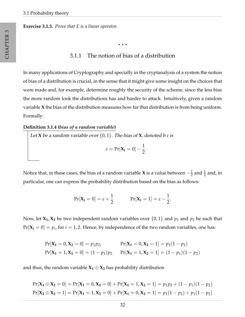
Exercise 3.1.3. Prove that E is a linear operator.

• • •

3.1.1 The notion of bias of a distribution

In many applications of Cryptography and specially in the cryptanalysis of a system the notion

of bias of a distribution is crucial, in the sense that it might give some insight on the choices that

were made and, for example, determine roughly the security of the scheme, since the less bias

the more random look the distributions has and harder to attack. Intuitively, given a random

variable X the bias of the distribution measures how far that distribution is from being uniform.

Formally:

Definition 3.1.4 (bias of a random variable)

Let X be a random variable over 0, 1. The bias of X, denoted b ε is

ε = Pr[Xi = 0]− 12

.

Notice that, in these cases, the bias of a random variable X is a value between −12 and 1

2 and, in

particular, one can express the probability distribution based on the bias as follows:

Pr[Xi = 0] = ε +12

Pr[Xi = 1] = ε− 12

.

Now, let X1, X2 be two independent random variables over 0, 1 and p1 and p2 be such that

Pr[Xi = 0] = pi, for i = 1, 2. Hence, by independence of the two random variables, one has:

Pr[X1 = 0, X2 = 0] = p1p2, Pr[X1 = 0, X2 = 1] = p1(1− p2)

Pr[X1 = 1, X2 = 0] = (1− p1)p2 Pr[X1 = 1, X2 = 1] = (1− p1)(1− p2)

and thus, the random variable X1 ⊕ X2 has probability distribution

Pr[X1 ⊕ X2 = 0] = Pr[X1 = 0, X2 = 0] + Pr[X1 = 1, X2 = 1] = p1p2 + (1− p1)(1− p2)

Pr[X2 ⊕ X2 = 1] = Pr[X1 = 1, X2 = 0] + Pr[X1 = 0, X2 = 1] = p1(1− p2) + p1(1− p2)

32

CH

AP

TE

R3

CH

AP

TE

R3


One can now derive the bias of this random variable from the bias ε1 and ε2 of X1 and X2

respectively, namely:

εX1⊕X2 = Pr[X1 ⊕ X2 = 0]− 12

= p1p2 + (1− p1)(1− p2)−12

=

(ε1 +

12

)(ε2 +

12

)+

(ε1 −

12

)(ε2 −

12

)= ε1ε2 +

12(ε1 + ε2) +

14+ ε1ε2 −

12(ε1 + ε2) +

14− 1

2

= 2ε1ε2.

In the next lemma it is generalized this result for a finite number of independent random

variables.

Lemma 3.1.4 (Piling-up lemma). Let X1, · · · , Xk be independent random variables over 0, 1. The

bias of the random variable X = X1 ⊕ · · · ⊕ Xk can be computed by the following formula:

εX = 2k−1k

∏i=1

εXi .

where εXi for 1 ≤ i ≤ k is the bias of the random variable Xi.

Proof: The proof of the lemma is done by induction on the number of independent random

variables considered.

(basis) The result is trivially verified when k = 1. Notice that the discussion above proves the

case k = 2.

(Step) Assume that for all l ≤ k the bias of X can be computed by the formula εX = 2k−1k

∏i=1

εXi

and assume that Let X1, · · · , Xk+1 are independent random variables over 0, 1. Then

X = X1 ⊕ · · · ⊕ Xk ⊕ Xk+1 = (X1 ⊕ · · · ⊕ Xk)⊕ Xk+1

Now it is used twice the hypothesis of induction. In the first case, the bias of X1 ⊕ · · · ⊕ Xk

is 2k−1k

∏i=1

εXi and thus applying the hypothesis of induction for k = 2 with the two random

distributions being X1 ⊕ · · · ⊕ Xk and Xk+1 one has:

εX = 2 · εX1⊕···⊕Xk · εXk+1 = 2 · 2k−1

(k

∏i=1

εXi

)· εXk+1 = 2k

k+1

∏i=1

εXi .

33

CH

AP

TE

R3

CH

AP

TE

R3

3.2 Entropy and information theory

as claimed.

Corollary 3.1.5. Let X1, · · · , Xk be independent random variables over 0, 1. If the bias of some the

random variable X = Xi then the bias of X1 ⊕ · · · ⊕ Xk cis also zero.

Notice that this results require the independence condition. The reader is invited to present

examples of non independent random variables in which the results above do not hold.

• • • • • • • • • • • • • • • • • • • • • • • • • • • • • • • • • • • • •

SECTION 3.2

Entropy and information theory

The reader is referred to the book [CT91] for a full comprehensive study of this thematic.

The concept of entropy is central in information theory and thus in cryptography. Heuristically

speaking, entropy is a measure to evaluate the uncertainty associated with a random variable

by the expected value of the information, usually counted in number of bits, and can be realized

as a function of the probability distribution inherent. The concept of entropy was introduced

by Claude E. Shannon in his seminal paper [Sha48] of 1948 entitled “A Mathematical Theory

of Communication”.

One can formally present the concept of entropy in an axiomatic way, as follows:

Definition 3.2.1

Let f be a function and let X, Y be finite random variables. In order to have f has a measure

of uncertainty then must satisfy:

Axiom 1: H(X) is non negative, that is, H(X) ≥ 0;

Axiom 2: H(X) must be continuos function;

Axiom 3: H(X) is maximum if X is the uniform distribution;

Axiom 4: H(X, Y) ≤ H(X) + H(Y) i.e., must be sub additive with the property that the

equality holds if and only if the variables are independent.

The first result that the interested reader can show is the following:

34

CH

AP

TE

R3

CH

AP

TE

R3


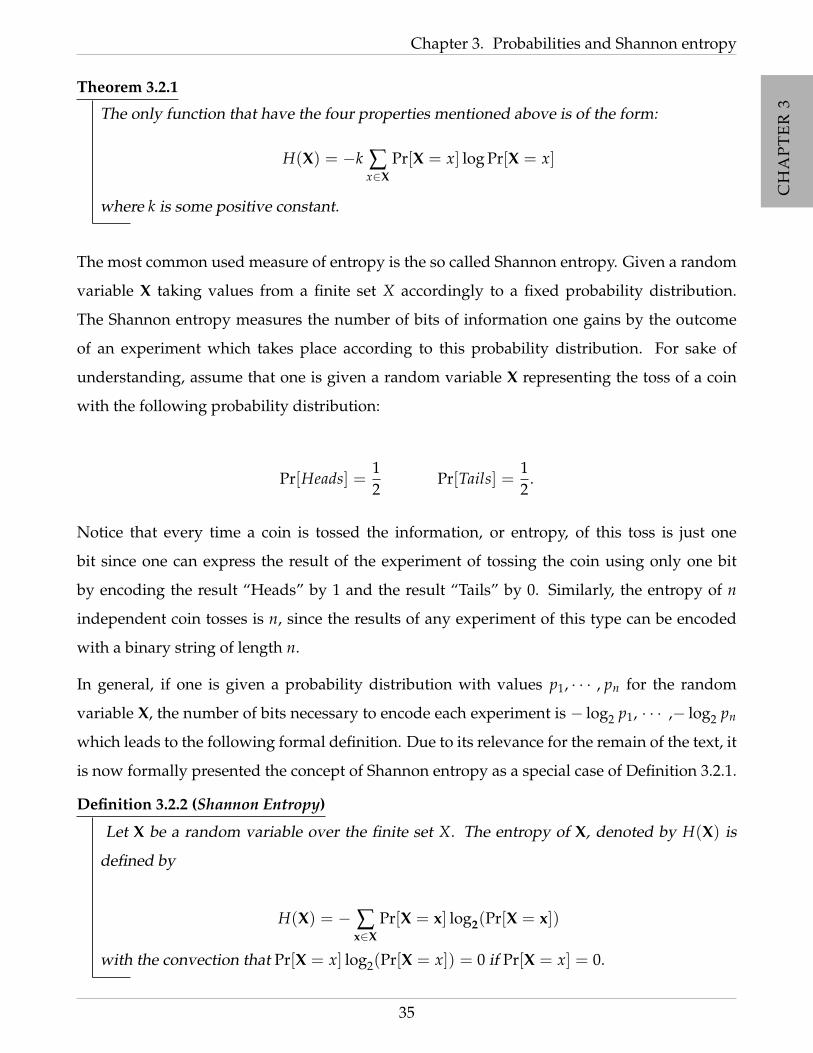
Theorem 3.2.1

The only function that have the four properties mentioned above is of the form:

H(X) = −k ∑x∈X

Pr[X = x] log Pr[X = x]

where k is some positive constant.

The most common used measure of entropy is the so called Shannon entropy. Given a random

variable X taking values from a finite set X accordingly to a fixed probability distribution.

The Shannon entropy measures the number of bits of information one gains by the outcome

of an experiment which takes place according to this probability distribution. For sake of

understanding, assume that one is given a random variable X representing the toss of a coin

with the following probability distribution:

Pr[Heads] =12

Pr[Tails] =12

.

Notice that every time a coin is tossed the information, or entropy, of this toss is just one

bit since one can express the result of the experiment of tossing the coin using only one bit

by encoding the result “Heads” by 1 and the result “Tails” by 0. Similarly, the entropy of n

independent coin tosses is n, since the results of any experiment of this type can be encoded

with a binary string of length n.

In general, if one is given a probability distribution with values p1, · · · , pn for the random

variable X, the number of bits necessary to encode each experiment is − log2 p1, · · · ,− log2 pn

which leads to the following formal definition. Due to its relevance for the remain of the text, it

is now formally presented the concept of Shannon entropy as a special case of Definition 3.2.1.

Definition 3.2.2 (Shannon Entropy)

Let X be a random variable over the finite set X. The entropy of X, denoted by H(X) is

defined by

H(X) = − ∑x∈X

Pr[X = x] log2(Pr[X = x])

with the convection that Pr[X = x] log2(Pr[X = x]) = 0 if Pr[X = x] = 0.

35

CH

AP

TE

R3

CH

AP

TE

R3


For example, if X is a uniform random variable over a set X with n elements, i.e., X is such that,

for all x ∈ X, Pr[X = x] = 1/n, then H(X) = n, which is the maximum value that the entropy

can take, since this is the most unpredictable possible distribution.

Lemma 3.2.1. Let X is a finite set and X a random variable. Then H(X) ≥ 0.

Proof: The thesis follows directly from the fact that 0 ≤ Pr[X = x] ≤ 1 for all x ∈ X, and also by

the convention assumed in Definition 3.2.2, which implies that Pr[X = x] log2(Pr[X = x]) ≤ 0.

Exercise 3.2.2. Let X be a finite set and X a random variable of X. Show that H(X) = 0 if and only if

the support of the probability distribution of X has only one element.

Exercise 3.2.3. Show that the function f (x) = log x in the interval [1, ∞[ is concave, i.e., for all

x, y ∈ [1, ∞[, f (λx + (1− λ)y) ≥ λ f (x) + (1− λ) f (y). Hint: Prove that the second derivative is

negative in the interval

Theorem 3.2.2 (Jensen’s inequality)

Let f be a continuous strictly concave function on an interval I. Let also ai > 0 be n values

such that

n

∑i=1

ai = 1.

Then, for all x1, · · · xn ∈ I:

n

∑i=1

ai f (xi) ≤ f

(n

∑i=1

aixi

)and the equality holds if and only if x1 = · · · = xn.

Proof: The proof is done by induction on the number n.

(Base:) For the case where n = 2, the inequality becomes a1 f (x1) + (1− a1) f (x2) ≤ f (a1x1 +

(1− a1)x2) which is true directly from the definition of concave function. The reader should

observe that in a concave function all points of the interval I are evaluated with a value that is

above the line defined by the points (x1, f (x1)) and (x2, f (x2)).

36

CH

AP

TE

R3

CH

AP

TE

R3


(Step:) Assume that the inequality is true for any n− 1 values, i.e., for any set of bi > 0 such

thatn−1

∑i=1

bi = 1,n−1

∑i=1

bi f (xi) ≤ f

(n

∑i=1

bixi

).

Let ai > 0 be n values such thatn−1

∑i=1

ai = 1 and consider a′i =ai

1− anfor i = 1, · · · n− 1. Then:

n

∑i=1

ai f (xi) = an f (xn) + (1− an)n−1

∑i=1

a′i f (xi).

Thus, applying the induction hypothesis on the second term one concludes that:

n

∑i=1

ai f (xi) ≤ an f (xn) + (1− an) f

(n−1

∑i=1

a′ixi

).

Now, from the fact that f is concave it follows that

n

∑i=1

ai f (xi) ≤ f

(anxn + (1− an)

n−1

∑i=1

a′ixi

)= f

(n

∑i=1

aixi

).

Theorem 3.2.3

Let X be a random variable over a finite set X = x1, · · · , xn such that the probability

distribution is Pr[x1] = p1, · · · , Pr[xn] = pn such that pi > 0 for all 1 ≤ i ≤ n. Then

H(X) ≤ log2 n and the equality holds, if and only if all pi = 1/n.

Proof: The proof follows directly from Jensen’s Inequality above applied to the function f (x) =

− log2(x) and with ai = pi. In fact:

H(X) = −n

∑i=1

pi log2 (pi)

=n

∑i=1

pi log2

(1pi

)

≤ log2

(n

∑i=1

pi1pi

)

= log2 n.

The equality holds, also by the Jensen’s Inequality, if and only if pi are all equal and thus equal

to 1/n.

37

CH

AP

TE

R3

CH

AP

TE

R3


Definition 3.2.3 (Joint entropy and conditional entropy)

Let X and Y be finite sets and X and Y be the two random variables associated with X and

Y respectively.

• The joint entropy of (X, Y), denoted by H(X, Y) is the entropy of the joint probability

distribution of X and Y i.e., defined by

H(X, Y) = − ∑x∈X

∑y∈y

Pr[x, y] log2(Pr[x, y]).

• The conditional entropy of Y given X, denoted by H(Y|X), is defined as the entropy

of the conditional distribution of Y given X i.e., it is defined by

H(Y|X) = ∑x∈X

Pr[x]H(Y|X = x)

= − ∑x∈X

Pr[x] ∑y∈y

Pr[y|x] log2(Pr[y|x])

= − ∑x∈X

∑y∈y

Pr[x, y] log2(Pr[y|x]).

Theorem 3.2.4 (Chain rule)

Let X and Y be two random variables. Then:

H(X, Y) = H(X) + H(Y|X)

Proof:

H(X, Y) = − ∑x∈X

∑y∈y

Pr[x, y] log2(Pr[x, y])

= − ∑x∈X

∑y∈y

Pr[x, y] log2(Pr[x]Pr[y|x])

= − ∑x∈X

∑y∈y

Pr[x, y] log2(Pr[x])− ∑x∈X

∑y∈y

Pr[x, y] log2(Pr[y|x])

= − ∑x∈X

Pr[x] log2(Pr[x])− ∑x∈X

∑y∈y

Pr[x, y] log2(Pr[y|x])

= H(X) + H(Y|X)

38

CH

AP

TE

R3

CH

AP

TE

R3


An important concept related with entropy in the mutual information I(X; Y) which can be

seen as the reduction in the uncertainty of X due to the knowledge of Y. Formally is defined as

follows:

Definition 3.2.4

Let X and Y be two random variables. The mutual information between X and Y is defined

by:

I(X; Y) = ∑x∈X

∑y∈y

Pr[x, y] log2

(Pr[x, y]

Pr[x]Pr[y]

).

Notice that

I(X; Y) = ∑x∈X

∑y∈y

Pr[x, y] log2

(Pr[x, y]

Pr[x]Pr[y]

)= ∑

x∈X∑y∈y

Pr[x|y] log2(Pr[x])

= − ∑x∈X

∑y∈y

Pr[x, y] log2(Pr[x])−(− ∑

x∈X∑y∈y

Pr[x, y] log2(Pr[x|y]))

= H(X)−H(X|Y)

Thus, mutual information can be expressed in terms of entropy. In the next exercise, the reader

is invited to explore further properties of entropy and mutual information.

Exercise 3.2.4. Let X, Y and Z be random variables. Show that:

1. If f is a function, then H [ f (X)] ≤ H [X];

2. H [X, Y] ≥ H [X] and H [X, Y] ≥ H [Y];

3. H [X|Y] ≤ H [X];

4. H [X|Y] = 0 if and only if X = f (Y) for some function f ;

5. H [X|Y] = H [X] if and only if X is independent of Y;

6. H [ f (X)|Y] ≤ H [X|Y];

7. H [X]| f (Y)] ≤ H [X|Y];

8. H [X, Y|Z] ≥ H [X|Z];

39

CH

AP

TE

R4

CH

AP

TE

R4

CH

AP

TE

R4CHAPTER 4

Notion of computational complexity

In this chapter it is settled the framework to deal with computational complexity issues. Nowa-

days modern cryptography is based on hard computational tasks that will be explained later in

the text. Contrarily to perfect secrecy, where one gets a system that is secure against all possible

attacks of an opponent in this approach the security that the parties rely on are hardness

computational assumptions and for that reason is not completely secure. One of the reasons

that cryptography is usually presented based on computational security and not on perfect

secrecy is due to the fact that for example, perfect security can only be achieved if the length

of the key is at least equal to the length of the message and the key cannot be used more than

once, which it is a severe drawback regarding “practical” cryptography. All these comparisons

and details will be clearer in due course. For the moment it is skipped further details regarding

security and it is presented the concept of computational complexity and all the topics inherent

to it that will be used in this work, like computational complexity classes and computational

hard assumptions.

41

CH

AP

TE

R4

CH

AP

TE

R4

CH

AP

TE

R4

4.1 Pseudo-code as base for computation

• • • • • • • • • • • • • • • • • • • • • • • • • • • • • • • • • • • • •

SECTION 4.1

Pseudo-code as base for computation

Several paradigms of computation can be used to introduce computational complexity. One of

the most common is the so called Turing machine model, that was proposed by Alan Turing in

1936 to formally present the notion of “procedure” and algorithm. In this work it is necessary to

present number theoretical algorithms, and Turing machines are not the most suitable model

to deal with such algorithms. For a general introduction to computability and complexity

it is referred to the reader the books [Sip12] and [?] (sernadas) and for the interested reader

in Turing machines and computational complexity based on this model it recommend the

reading, for example, of [AB09] or [Pap94].

The model used is almost irrelevant for the study of complexity since the models are equiv-

alent. To define complexity one needs to specify an algorithm, which is the mechanism to

solve computational task or problems. In this work instead of using any specific programming

language and instead it will be used the notion of pseudocode, which is a very high level

description of an algorithm. More or less it is a language very close to the human language that

describes with a specific instructions actions that one wants to describe or intend the algorithm

to do. For example, if one wants to do a conditional action on a number n (say divide it by

two) if it is even and another action otherwise (say sum 1 and divide it by two) and keep it in

a variable x one can represent it in the following way:

If n is even then x = n/2 else x = (n + 1)/2.

Notice that just from the reading of the instruction given above the reader without knowing

anything about programming can understand that the intention is that given a number do a

certain operation if it is even or odd.

In the sequel it is presented the nomenclature that will be used in this book. If the reader thinks

about an algorithm (as a recipe) there are several common components that are essential for its

description. One needs:

42

CH

AP

TE

R4

CH

AP

TE

R4

CH

AP

TE

R4

Chapter 4. Notion of computational complexity

Pseudo-code syntax

Input: The data that are given to the algorithm to perform actions;1

Output: The expected value that will be given by the algorithm at the end;2

Variable declaration: Usually are letters or simple expressions that are easy to remember

their meaning and are used for intermediate calculations or instructions;

Body command: In this part the execution instructions are written as described below us-

ing terms and commands containing only variables and input and outputs..

Terms

Arithmetical terms: All basic operations are inbuilt in the code, +, −, /; Another

important operations that will play a central role in the rest of the book are the (mod )

operation that returns the remainder of a integer division and the div that returns the

integer division.

Boolean terms: This term is used to designate operations of comparison, such as, =,

6=, ≤, <, ≥ and >. It is included also the disjunction and the conjunction operations and

and or respectively.

Commands

Attributions: It is the action of given to a variable a certain value;

Random sample: Given a finite set, it chooses randomly (with uniform distribution)

an element of that set;

Sequential composition: It has the form of

(command 1) ;

(command 2);

with the intend interpretation that command 1 is executed and then command 2 is exe-

cuted.1In the example given above, the input could be for example 4 which should be kept in n;2In the example given above, the output is the value of x;

43

CH

AP

TE

R4

CH

AP

TE

R4

CH

AP

TE

R4

4.1 Pseudo-code as base for computation

Alternative composition: It has the form

If (boolean term) then (command) else (command)

with the canonical interpretation, i.e., one test if the expression is true or false. In the

former case it is performed the commands in then part and the latter one it is performed

the commands on the else part;

Bounded iterative composition (For): This an element that allows to perform a set of

instructions that are meant to be repeated a fixed number of times, like the name suggests.

The structure involves a variable, say i, and is as follows:

For i from 1 to (number) do (command).

In the command part it is mandatory to increment the variable i in order to be able to rich

the end of the cycle;

Iterative composition (While): This an element that allows to perform repeatedly a

set of instructions while a certain condition is true. Contrarily to the bounded iterative

composition, the number of time that the cycle is executed is not fixed a priori. The

structure is:

While (boolean term) do (command).

In the command part it is mandatory to include a command that might change the con-

dition in order to possibly break the cycle.

Some considerations are also needed. For example, given a variable x, the expression x = x+ 1,

is used to designate an actualization of the variable, i.e., to the variable x it is given the value

that was already in that variable plus one. Notice that once the variable has been actualized

than the previous value of x is lost.

Now it is presented an example of a pseudo code. It is described a basic operation for which one

has an inbuilt function. Given two non zero natural numbers n and m as input it determines

the integer division of n by m.

44

CH

AP

TE

R4

CH

AP

TE

R4

CH

AP

TE

R4


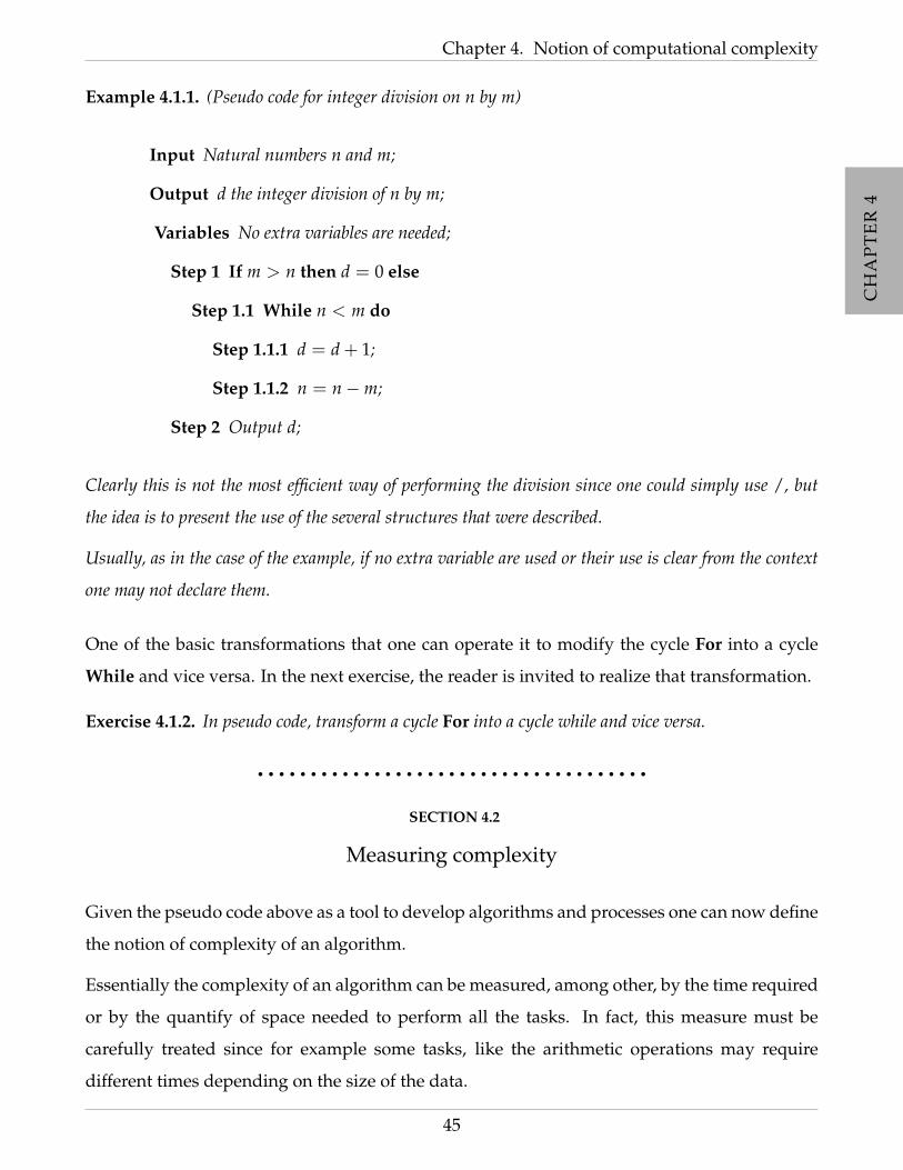
Example 4.1.1. (Pseudo code for integer division on n by m)

Input Natural numbers n and m;

Output d the integer division of n by m;

Variables No extra variables are needed;

Step 1 If m > n then d = 0 else

Step 1.1 While n < m do

Step 1.1.1 d = d + 1;

Step 1.1.2 n = n−m;

Step 2 Output d;

Clearly this is not the most efficient way of performing the division since one could simply use /, but

the idea is to present the use of the several structures that were described.

Usually, as in the case of the example, if no extra variable are used or their use is clear from the context

one may not declare them.

One of the basic transformations that one can operate it to modify the cycle For into a cycle

While and vice versa. In the next exercise, the reader is invited to realize that transformation.

Exercise 4.1.2. In pseudo code, transform a cycle For into a cycle while and vice versa.

• • • • • • • • • • • • • • • • • • • • • • • • • • • • • • • • • • • • •

SECTION 4.2

Measuring complexity

Given the pseudo code above as a tool to develop algorithms and processes one can now define

the notion of complexity of an algorithm.

Essentially the complexity of an algorithm can be measured, among other, by the time required

or by the quantify of space needed to perform all the tasks. In fact, this measure must be

carefully treated since for example some tasks, like the arithmetic operations may require

different times depending on the size of the data.

45

CH

AP

TE

R4

CH

AP

TE

R4

CH

AP

TE

R4

4.2 Measuring complexity

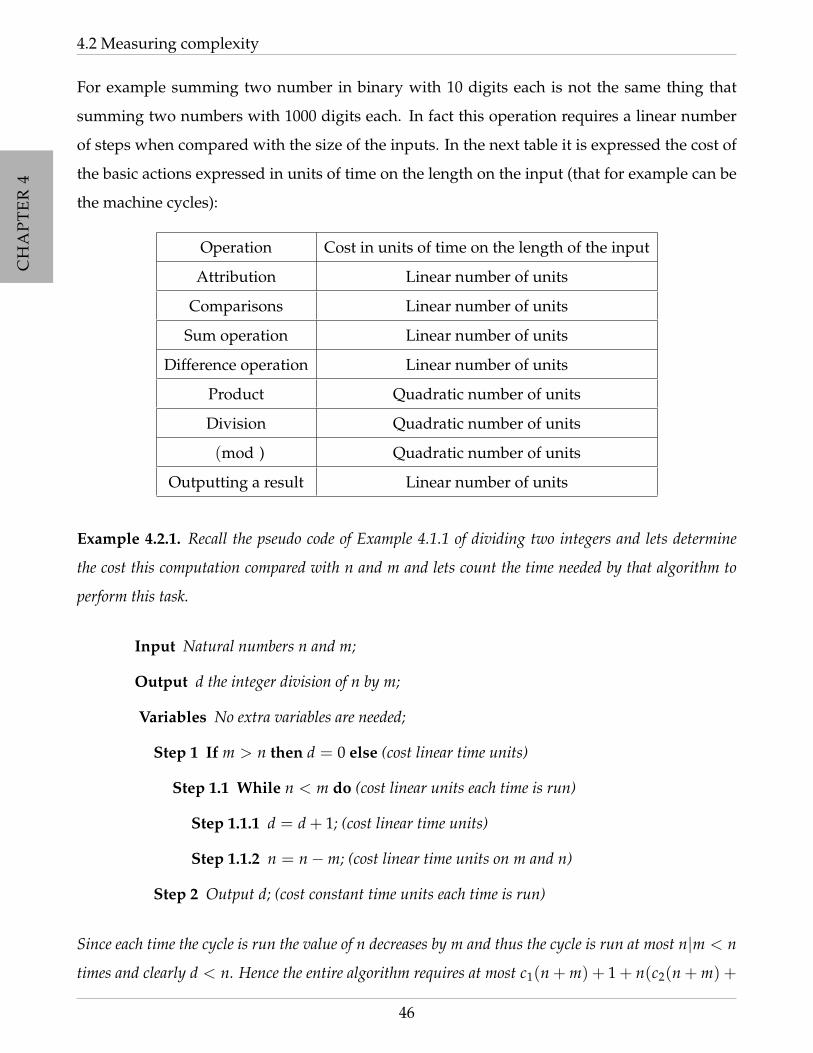
For example summing two number in binary with 10 digits each is not the same thing that

summing two numbers with 1000 digits each. In fact this operation requires a linear number

of steps when compared with the size of the inputs. In the next table it is expressed the cost of

the basic actions expressed in units of time on the length on the input (that for example can be

the machine cycles):

Operation Cost in units of time on the length of the input

Attribution Linear number of units

Comparisons Linear number of units

Sum operation Linear number of units

Difference operation Linear number of units

Product Quadratic number of units

Division Quadratic number of units

(mod ) Quadratic number of units

Outputting a result Linear number of units

Example 4.2.1. Recall the pseudo code of Example 4.1.1 of dividing two integers and lets determine

the cost this computation compared with n and m and lets count the time needed by that algorithm to

perform this task.

Input Natural numbers n and m;

Output d the integer division of n by m;

Variables No extra variables are needed;

Step 1 If m > n then d = 0 else (cost linear time units)

Step 1.1 While n < m do (cost linear units each time is run)

Step 1.1.1 d = d + 1; (cost linear time units)

Step 1.1.2 n = n−m; (cost linear time units on m and n)

Step 2 Output d; (cost constant time units each time is run)

Since each time the cycle is run the value of n decreases by m and thus the cycle is run at most n|m < n

times and clearly d < n. Hence the entire algorithm requires at most c1(n + m) + 1 + n(c2(n + m) +

46

CH

AP

TE

R4

CH

AP

TE

R4

CH

AP

TE

R4


c3d + c4n) where ci are some constants. Hence asymptotically computing the division of two integers n

by m costs, in terms of time units n2 + nm.

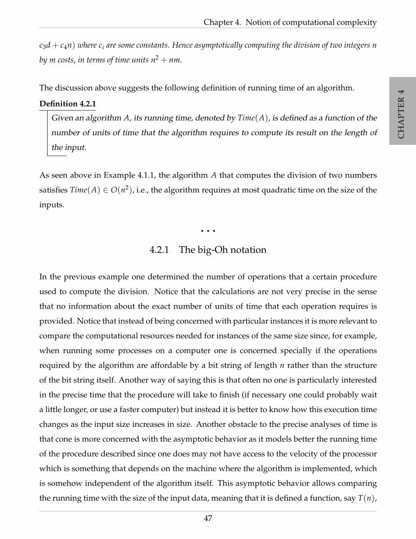
The discussion above suggests the following definition of running time of an algorithm.

Definition 4.2.1

Given an algorithm A, its running time, denoted by Time(A), is defined as a function of the

number of units of time that the algorithm requires to compute its result on the length of

the input.

As seen above in Example 4.1.1, the algorithm A that computes the division of two numbers

satisfies Time(A) ∈ O(n2), i.e., the algorithm requires at most quadratic time on the size of the

inputs.

• • •

4.2.1 The big-Oh notation

In the previous example one determined the number of operations that a certain procedure

used to compute the division. Notice that the calculations are not very precise in the sense

that no information about the exact number of units of time that each operation requires is

provided. Notice that instead of being concerned with particular instances it is more relevant to

compare the computational resources needed for instances of the same size since, for example,

when running some processes on a computer one is concerned specially if the operations

required by the algorithm are affordable by a bit string of length n rather than the structure

of the bit string itself. Another way of saying this is that often no one is particularly interested

in the precise time that the procedure will take to finish (if necessary one could probably wait

a little longer, or use a faster computer) but instead it is better to know how this execution time

changes as the input size increases in size. Another obstacle to the precise analyses of time is

that cone is more concerned with the asymptotic behavior as it models better the running time

of the procedure described since one does may not have access to the velocity of the processor

which is something that depends on the machine where the algorithm is implemented, which

is somehow independent of the algorithm itself. This asymptotic behavior allows comparing

the running time with the size of the input data, meaning that it is defined a function, say T(n),

47

CH

AP

TE

R4

CH

AP

TE

R4

CH

AP

TE

R4


that expresses how the time requirements depends on inputs of size n.

All the above arguments motivate the introduction of the big-Oh, which formally expresses

the idea that, rather than describing exactly the function T(n) of number of cycle units for

the execution time, one can instead describe the so called rate of growth of the time func-

tion. Accordingly to all the arguments above, this notation provides a description of resource

requirements of an algorithm that is (usually) independent of computational model and of

implementation platform and describes exactly how one must increases the resources available

as the input size increases. This is frequently the most relevant and informative information

about an algorithm’s behavior.

Lets consider the general example presented in the Example 4.2.1. The calculations determined

that the total cost is approximately equal to T(n, m) ≈ c1(n+m)+ 1+n(c2(n+m)+ c3d+ c4n),

which will be of the order of nm + n2, and will be denoted by O(nm + n2) which avoids over-

loaded notation and a more concise representation of the idea of the time that the algorithm

will take to finish.

Definition 4.2.2 (The big-Oh notation)

Let f , g : N→ [0, ∞) be two functions. One says that:

• f ∈ O(g) if there is a constant c > 0 such that f (n) ≤ c · g(n), for almost all n ∈ N.

• f ∈ Ω(g) if there is a constant c > 0 such that f (n) ≥ c · g(n), for almost all n ∈ N.

• f ∈ Θ(g) if and only if f ∈ O(g) and f ∈ Ω(g).

• f ∈ o(g) if for any constant c > 0 and for sufficiently large n ∈ N, f (n) ≤ c · g(n).

• f ∈ ω(g) if for any constant c > 0 and for sufficiently large n ∈ N, f (n) ≥ c · g(n).

Some of the most used bounds are: O(1) called constant, O(log n) called logarithmic, nO(1)

called polynomial, 2no(1)called sub-exponential and 2nO(1)

called exponential.

In the next table it is referred in the Big-oh notation the cost of the basic operations of the

Pseudo codes in order to establish the bounds of algorithms:

48

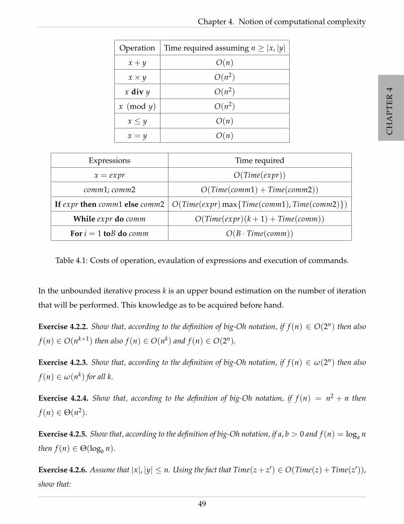
CH

AP

TE

R4

CH

AP

TE

R4

CH

AP

TE

R4


Operation Time required assuming n ≥ |x, |y|

x + y O(n)

x× y O(n2)

x div y O(n2)

x (mod y) O(n2)

x ≤ y O(n)

x = y O(n)

Expressions Time required

x = expr O(Time(expr))

comm1; comm2 O(Time(comm1) + Time(comm2))

If expr then comm1 else comm2 O(Time(expr)maxTime(comm1), Time(comm2))

While expr do comm O(Time(expr)(k + 1) + Time(comm))

For i = 1 toB do comm O(B · Time(comm))

Table 4.1: Costs of operation, evaulation of expressions and execution of commands.

In the unbounded iterative process k is an upper bound estimation on the number of iteration

that will be performed. This knowledge as to be acquired before hand.

Exercise 4.2.2. Show that, according to the definition of big-Oh notation, if f (n) ∈ O(2n) then also

f (n) ∈ O(nk+1) then also f (n) ∈ O(nk) and f (n) ∈ O(2n).

Exercise 4.2.3. Show that, according to the definition of big-Oh notation, if f (n) ∈ ω(2n) then also

f (n) ∈ ω(nk) for all k.

Exercise 4.2.4. Show that, according to the definition of big-Oh notation, if f (n) = n2 + n then

f (n) ∈ Θ(n2).

Exercise 4.2.5. Show that, according to the definition of big-Oh notation, if a, b > 0 and f (n) = loga n

then f (n) ∈ Θ(logb n).

Exercise 4.2.6. Assume that |x|, |y| ≤ n. Using the fact that Time(z+ z′) ∈ O(Time(z)+ Time(z′)),

show that:

49

CH

AP

TE

R4

CH

AP

TE

R4

CH

AP

TE

R4


1. x× y ∈ O(n2);

2. x (mod y) ∈ O(n2);

3. x divy ∈ O(n2);

as claimed and expressed in the Table 4.1. As a curiosity, one can perform, using Fourier transforma-

tions, the multiplication in time of O(n log n).

• • •

4.2.2 Complexity classes

In this section it is introduced the notion of complexity classes. They are important as they

catalogue the problems in families for which similar resources are needed to computer their

solutions. Three of the most important ones that will be used in this text are the classes P,

NP and BPP. The former one characterizes the family of problems for which one can find in

polynomial time (on the length of the input) a solution. The second one characterizes the class

of problems for which, given a solution, one can verify in polynomial time that it is really a

solution, and the latter one, nowadays classified of feasible problems, is the class of problems

that, using some randomness, is able to find a solution for a problem with a small probability

of error in polynomial time.

It might seem to the reader that all this classes are similar, and in fact, they are, but they

are also fonts of problems that are in the border line of human knowledge, in the sense that,

many relationships between them are unknown and, for example, are part of the millennium

problems. The differences between these two classes are fundamental. Without resources

restrictions, checking if a given solution is in fact a solution and searching for a solutions are

equivalent but, in the bounded resource models it is unknown if they are equivalent or not.

This equivalence is known as the famous problem P versus NP.

The difference of searching and checking is crucial for the modern cryptography that will be

studied in detail later on this course. Since 1970, all basic cryptographic constructions and

applications are founded in computational hardness assumptions similar to the one discussed

above. For example, as it will be discussed in detail in due course, under reasonable assump-

tion of complexity, there are functions for which one can compute its value efficiently given the

50

CH

AP

TE

R4

CH

AP

TE

R4

CH

AP

TE

R4


input, but there are no feasible ways of inverting it, or simply given an element in the range

of the function to find one of it pre-image. A candidate for such function is the multiplication

of two prime numbers. It is very easy to compute the product of two primes, but given a

number that is composed of product of two primes, finding those two primes is believed to be

infeasible. It is worthwhile to mention that even if P = NP, i.e. , in a scenario where checking

is equivalent to searching, it is uncertain the existence of such functions. On the other hand if

such functions do exist then, as it will be proved, P = NP.

To formally present all these computational complexity classes one need some technical defi-

nitions. After the proper definitions of these complexity classes some relationships are estab-

lished and explained.

Definition 4.2.3 (Input size)

Given a program P with input x1 . . . xk, the input size |(x1 . . . xk)| corresponds tok

∑i=1|xi|

where |xi| is the number of bits required to represent the input xi. In most cases the inputs

are non-negative integers and so, |xi| is the number of bits in binary representation, that is

|xi| = dlog(xi + 1)e.

Definition 4.2.4 (Polynomial-time algorithm)

Given a program P with input x1 . . . xk, one says that P is polynomial-time on (part of

the) inputs xi1 , . . . , xi` , with xij ∈ x1 . . . xk, if Time(P) ∈ O(p(|xi1 |, . . . , |xi` |)) for some

polynomial p.

An algorithm is said to be polynomial-time if it is polynomial time on all its inputs.

A function is said to be polynomial-time (on some inputs) if there is an polynomial-time

(on some inputs) algorithm that computes it.

Definition 4.2.5 (Polynomial-time set and the classP)

Let A ⊆ Nk, A is said to be polynomial time if there is a polynomial-time algorithm to

compute its indicator function χA : Nk → 2.

The class of all polynomial-time sets is denoted by P.

Example 4.2.7. In this example, one proves that the set of even numbers is in P.

Consider E = x ∈ N : x is even and consider the following algorithm to compute E :

51

CH

AP

TE

R4

CH

AP

TE

R4

CH

AP

TE

R4


Algorithm 4.2.8 (A)

Input: x

Output: 0 if x is odd and 1 is even

Step 1: r = 1− x (mod 2);

Step 2: Output r;

Notice that Time(A) ∈ O(n2), where |x| = n and taking fA as the function computed byA, fA = χE .

Thus, accordingly to Definition 4.2.5 E ∈ P.

Exercise 4.2.9. Show that:

1. Psquare = x ∈ N : x is a perfect square ∈ P;

2. Ppower = x ∈ N : x is a perfect power ∈ P;

3. Primes = x ∈ N : x is a prime number ∈ P

Definition 4.2.6 (Non-deterministic polynomial-time set)

Let A ⊆ Nk, A is said to be non-deterministic polynomial time, if there is fA : Nk+1 → 2

which is polynomial-time in the first k inputs and fulfills the following conditions:

• there exists w ∈ N such that fA(x1, . . . , xk, w) = 1 if (x1 . . . , xk) ∈ A;

• for all w ∈ N fA(x1, . . . , xk, w) = 0 if (x1 . . . , xk) 6∈ A.

In these conditions, fA is said to be a certification function for A. The class of all non-

deterministic polynomial-time sets is denoted by NP.

Exercise 4.2.10 (P ⊆ NP). Show that if A is in P then A is in NP.

Example 4.2.11. It will be proved that the following set is in NP:

A = (x, y) ∈ N2 : ∃k > 1, k < y ∧ k|x.

52

CH

AP

TE

R4

CH

AP

TE

R4

CH

AP

TE

R4


To prove that A ∈ NP one has to describe the certification function fA. Consider the following definition

of fA:

fA(x, y, w) =

1 if w|x ∧ 1 < w < y

0 otherwise

Notice that computing f implies only testing either w|x which is quadratic on x (if w > x one can reject

it automatically) and comparisons involving w and y which, since w ≤ y is linear on w. Thus, fA is

in fact computable in polynomial time. Also notice that fA(x, y, w) = 1 if and only if x, y ∈ A and the

witness, in the affirmative case, is, in fact, k defined in A.

From the previous exercise the reader can easily derive that the problem of factorization is also

NP. In fact, if A was computable in polynomial time then with a bijection argument querying

fA adaptively, fA(x, x/2), f (x, x/4), f (x, x/8) or f (x/3x/8) and so on... The total number of

queries is log(x) which makes the algorithm for factoring polynomial. The interested reader

can in fact also design directly a certification function for factoring and deduce that function

can be used to compute A.

One of the most important problem in Mathematics and Theoretical Computer Science is to

determine whether P = NP. This problem is classified by the Clay Institute as one of the

millennium problem worthing a 1 million dollar price. All the modern cryptography that is

used in practice since the 70’s is based on the fact that some specific functions exist which, if

P = NP, then they cannot exist. These function will be presented in next section. The question

P = NP basically wonders if having an easy, i.e. efficient, process of verifying if a solution is

indeed a solution is equivalent of finding that solution also efficiently. This formalism is now

explained in the next definitions and proposition.

Definition 4.2.7 (Decision version ofP =NP)

For each set A in NP there is a polynomial-time algorithm that computes χA.

53

CH

AP

TE

R4

CH

AP

TE

R4

CH

AP

TE

R4


Definition 4.2.8 (Search version ofP =NP)

For each set A ⊆ Nk in NP with certification polynomial-time function fA, there exists a

polynomial-time function gA : Nk → N such that:

• fA(x1, . . . xk, gA(x1, . . . xk)) = 1 if (x1, . . . xk) ∈ A;

• fA(x1, . . . xk, gA(x1, . . . xk)) = 0 if (x1, . . . xk) 6∈ A.

Theorem 4.2.1 (Equivalence between decision and search version ofP =NP)

The two definitions of P = NP given in definitions 4.2.7 and 4.2.8 above are equivalent.

This theorem in fundamental from the cryptographic point of view as it states in two different

ways the same problems. In some cases, the use of a particular definitions gives a more natural

intuition on the result that one wants to prove.

Proof:

(Definition 4.2.8⇒ Definition 4.2.7 i.e., Search implies Decision)

Assume that A is a set inNP for which there exists a certification function fA and a polynomial

time function g such that f (x1, . . . xk, g(x1, . . . xk)) = 1 if and only if (x1, . . . xk) ∈ A.

In order to prove that A fulfills the Definition 4.2.7, one needs to show that there exists a poly-

nomial time algorithm that computes its characteristic sequence. Take the following algorithm:

Algorithm 4.2.12 (B to compute χA)

Input: (x1, . . . , xk) ∈ Nk, fA and gA;

Output: χA(x1, . . . , xk);

Step 1: x = gA(x1, . . . , xk);

Step 2: y = fA(x1, . . . , xk, x);

Step 2: Output y

54

CH

AP

TE

R4

CH

AP

TE

R4

CH

AP

TE

R4


Since fA(x1, . . . xk, gA(x1, . . . , xk)) = 1 if and only if (x1, . . . xk) ∈ A then B, on an input

(x1, . . . , xk) computes exactly χA.

Notice also that B is also polynomial time on the input since gA and fA are polynomial-time

computable and the output operation is also polynomial, thus Time(B) ∈ O(p) for some

polynomial p.

(Definition 4.2.7⇒ Definition 4.2.8 i.e., Decision implies Search)

Assume without loss of generality that A is a subset ofN that is inNP accordingly to Definition

4.2.6. Assume also that there is a polynomial-time algorithm that computes χA, i.e., A satisfies

the conditions of Definition 4.2.7.

Consider a set A such that (x, y, z) ∈ A if and only if there is a w written in binary with z digits

such that fA(x, e−1(e(y).w)) = 1 where fA is the certification function of A, e is the polynomial

time bijection with polynomial time inverse 3 between

a : ∃n ∈ N such that a = a1 . . . an ∧ ai ∈ 0, 1

and N and · is used to describe the binary concatenation of two strings.

Claim 4.2.13. A ∈ NP.

To prove the claim just apply the Definition 4.2.6 of NP with the function f A defined by

f A(x, y, (w, z)) = fA(x, e−1(e(y).w)) as constructed above. Notice that f has 2 extra arguments

but, since e and its inverse, and also fA are polynomial time computable on x, y, the function

f A is a certification function.4

From the fact that A ∈ NP one can conclude, accordingly to Definition 4.2.7 that χA is com-

putable in polynomial time.

To prove that A is in the conditions of Definition 4.2.8 one needs to define a certification

function f for which there exists a polynomial-time function g such that:

3The reader is invited to give the details of this bijection and prove that, in fact, can be computed in polynomial

time and its inverse is also polynomial.4In Definition 4.2.6 the function must have only one argument. It is left to the interested reader to verify that if

one defines NP with k + l arguments as in Definition 4.2.6, where l is some fixed value, then the two definitions

ofNP coincide.

55

CH

AP

TE

R4

CH

AP

TE

R4

CH

AP

TE

R4

4.3 One-way functions

f (x, g(x)) = 1 if and only if x ∈ A.

One defines g as the function computed by the following algorithm:

Algorithm 4.2.14 (to compute g(x))

Input: x ∈ N, χA, fA and χtildeA;

Output: g(x);

Step 1: If χA(x) = 1 then

Step 1.1: w = ε;

Step 1.2: While fA(x, w) = 0 do

Step 1.2.1: If χA(x, w.1) = 1 then

Step 1.2.1.1: w = w.1;

Step 1.2.1.2: else w = w.0;

Step 2: w = ε;

Step 3: Output w

Notice that this algorithm terminates in polynomial time as the operations involved are all

polynomial and from the fact that, since A ∈ NP, there exist a witness w of polynomial size.

• • • • • • • • • • • • • • • • • • • • • • • • • • • • • • • • • • • • •

SECTION 4.3

One-way functions

In this section some formal definitions of different one-way functions are presented and then it

is briefly discussed some candidates that are widely believed to be one-way functions. Heuris-

tically speaking a function is said to be one way if it is easy to compute on every input, but

56

CH

AP

TE

R4

CH

AP

TE

R4

CH

AP

TE

R4


relatively hard to invert given an element on the range of a random input. Accordingly to

previous section the terms ”easy” and ”hard” are understood under computational complexity

theory, namely the theory of polynomial time problems.

For the reader that is not familiar with the concept of one way functions it might be strange

the fact that one can talk about one way functions that are not one-to-one since one requires

that it has inverse. In fact, this constrain is not mandatory and almost all candidates are not

one-to-one. It also clear that one-to-one requirement is not sufficient to be one way, since the

identity is clearly an example of it.

Definition 4.3.1

A function f : N → N is honest if | f (x)| and |x| are polynomially related, i.e., for some

k > 0 and for every x ∈ Σ?,

(| f (x)| ≤ |x|k + k) ∧ (|x| ≤ | f (x)|k + k).

Now it is presented the notion of one-way function:

Definition 4.3.2 (One-way function)

A function f : N→ N is said to be a one-way function if:

• f is honest;

• f is computable in polynomial time;

• f−1 is not computable in polynomial time;

The first result one might prove is that, in fact, if one-way functions exist, then, P 6= NP. The

reciprocate of this statement is not true. Even ifP 6= NP it might be case that one-way function

do not exist.

Theorem 4.3.1

If one-way functions as presented in Definition 4.3.2, then P 6= NP.

Proof : The proof is carried over by contraposition.

Assume that P = NP and let f be a honest bijection that is computable in polynomial time. The goal is

57

CH

AP

TE

R4

CH

AP

TE

R4

CH

AP

TE

R4


to show that f−1 is also computable in polynomial time. Consider the following set:

A = (y, x) ∈ N2 : ∃z such that f (e−1(e(x) · z)) = y

where e is again the polynomial time bijection betweenN and 0, 1∗ and e(x) · z is again an abbreviation

for the concatenation os binary strings.

First one needs to prove that A ∈ NP. To do that, one needs to compute a certification function h : N3 →

0, 1 for A, i.e., that is computable in polynomial time in the first two arguments and h(y, x, w) = 1 if

and only if (y, x) ∈ A.

Consider

h(y, x, w) =

1 if f (e−1(e(x) · z)) = y

0 otherwise

Then h is polynomial in (y, x) since f is polynomial time computable and f is honest. In fact, the absolute

value of |e−1(e(x)) · z| − |y|, since f is honest, is polynomial bounded by |y|. It is then easy to verify that

h is a certification function for A.

Since A ∈ NP there exists a polynomial time computable function g with g(y, x) = w satisfying

h(y, x, g(y, x)) = 1 if and only if (y, x) ∈ A. By the Search version of the problem P = NP of Definition

4.2.8 g is computable in polynomial time. If one considers f−1(y) = g(y, e−1(ε)) then f−1 is, in fact,

computable in polynomial time and is the inverse of f . Notice that if g(y, e−1(ε)) = w then f (w) = y. In

fact, g(y, e−1(ε)) = w means that h(y, e−1(ε), w) = 1 which is equivalent to say that:

y = f (e−1(e−1(e−1(ε) · e(w))) = f (e−1(ε · e(w)))) = f (e−1(e(w))) = f (w)

which means that g is in fact the inverse of f .

As it will be seen later, the existence of one-way functions is not enough to guarantee that

one can design a public key cryptographic systems as they, bey themselves, do not ensure the

existence of an easy way of decrypting a message that was ciphered with a one-way function.

In order to achieve that goal one will need the notion of a trapdoor one way function. Intu-

itively, these functions are one-way function but with a ”backdoor” that allows the decryption

efficiently in the presence of a secret.

58

CH

AP

TE

R4

CH

AP

TE

R4

CH

AP

TE

R4


Definition 4.3.3 (trapdoor one-way function is a one-way function)

A function f : N→ N is said to be a trapdoor one-way function if it is a one-way function

with the additional property that given some extra information, usually called the trapdoor

information, it becomes feasible to find for any given y in the range of f one its pre images,

i.e., exists a function g : N2 → N computable in polynomial time for which there exists a

sequence of secrets (sn)− n ∈ N such that g(y, s|y|) = x and y = f (x).

Notice that if sn was computational easy to obtain then f would not be a one-way function.

This result is expressed in the next proposition which formal proof is left for the interested

reader.

Proposition 4.3.1. Let f be a trapdoor one-way function and (sn)n∈N as in the previous definition.

Then s|y| cannot be computed in polynomial even with the knowledge of f .

There are other several definitions that one can adopt as one-way functions, based on prob-

abilistic algorithms that are essentially similar to the one presented above. Here they are

presented with the intuit to be a more complete reference for the reader. The different between

the definitions presented bellow concerns the security requirements made.

In all definitions of the rest of the section it is assumed that f is honest. As it will be seen later

on, the requirement of honesty of f cannot be avoided in order to define properly one-way

functions that are not trivially one-way due to the fact that the function compress to much.

The weakest version of one-way functions considered in the literature is based on opponents

that only have deterministic polynomial time resources to try to invert the function.

59

CH

AP

TE

R4

CH

AP

TE

R4

CH

AP

TE

R4


Definition 4.3.4 (Deterministic one-way function)

An honest function f : Σ∗ → Σ∗ is a deterministic one-way function if the following two

conditions hold:

Easy to compute: there is a (deterministic) polynomial time algorithm A such that on

every input x, the algorithm A outputs f (x) (i.e., A(x) = f (x)).

Slightly hard to invert: for any deterministic polynomial time algorithm B, for some

polynomial q(·), for every sufficiently large n,

Prx∈Σn [ f (B( f (x), n)) 6= f (x)] >1

q(n).

If one allows some access to randomness to the opponents it is possible to define two other

variants of one-way functions.

In the case of a strong one-way function, it is required that the inversion happens with low

probability and in the weak version the non inversion must happen with non-negligible prob-

ability.

Definition 4.3.5 (Weak one-way function)

An honest function f : Σ∗ → Σ∗ is a weak one-way function if the following two conditions

hold:



Slightly hard to invert: for any polynomial t(·), there is a polynomial q(·) such that for

every probabilistic t-time-bounded algorithm B and for every sufficiently large n,

Pr(x,r)∈Σn×Σt(n) [ f (B( f (x), r, n)) 6= f (x)] >1

q(n).

60

CH

AP

TE

R4

CH

AP

TE

R4

CH

AP

TE

R4


Definition 4.3.6 (Strong one-way function)

An honest function f : Σ∗ → Σ∗ is a strong one-way function if the following two condi-

tions hold:



Hard to invert: for any polynomial t(·), for every probabilistic t-time-bounded algo-

rithm B, for every positive polynomial q(·), and for every sufficiently large n,

Pr(x,r)∈Σn×Σt(n) [ f (B( f (x), r, n)) = f (x)] <1

q(n).

In the previous definitions, r denotes the randomness used by the algorithm B and its length is

bounded by its running time.

It is easy to see that any weak one-way function is a deterministic one-way function and that

any strong one-way function is a weak one-way function and is left as an exercise for the

interested reader.

Exercise 4.3.2. Let f be an honest function. Show the following statements:

1. If f is a strong one-way function then f is also a weak one-way function.

2. If f is a weak one-way function then f is also a deterministic one-way function.

3. Conclude that if f is a strong one-way function then f is also a deterministic one-way function.

Exercise 4.3.3. Show that if f is an one-way function then f cannot have a polynomial sized range, i.e.,

for every polynomial p there exists an infinite many n for which # f (x) : x ∈ 0, 1n > p(n).

Exercise 4.3.4. Show that if f is a one-way function then g = f f is also a one way function.

Exercise 4.3.5. Show that if f and g are two weak one-way functions then their composition may not

be a one way function.

The reader may be puzzled by the requirement of honesty of f in the definitions of one-way

functions. To make clear the importance of this requirement it is presented the next example.

61

CH

AP

TE

R4

CH

AP

TE

R4

CH

AP

TE

R4


Example 4.3.6. Consider the following function f :

f : 0, 1∗ → 0, 1∗

x = x[1:n] → y = x[1:log n]

I.e., the function that given an input x only outputs the first logarithmic of its bits. Clearly, this function

is not honest, as it exponentially compressed the input. To understand that f could in fact be a one-way

function just observe that given y of length log n, printing for example x = y0...0 of length n (that

is a pre image of y by f ) any algorithm requires at least O(n) computational steps, but O(n) is not

polynomial on the size of y which is log(n).

A fundamental question regarding one-way functions is their relationships. For instance, in

the previous exercise, one showed that strong one-way functions are in fact stronger than the

weak one-way functions, in the sense that the existence of the former implies the existence of

the latter, but nothing is said about the opposite. In the next example it is shown that several

weak one-way functions might not be a strings one, but later on, one proves that the existence

of weak one-way functions imply the existence of weak one-way functions by a constructive

argument.

Example 4.3.7. Assume that f : 0, 1∗ → 0, 1∗ is a strong one-way function and consider the

following function g:

g : 0, 1∗ → 0, 1∗

x →

0 f (x) if x starts with 0

x if x starts with 1

Clearly g is not a strong one-way function since in the case that one has as an image y which the first

bit is 1 then it is easy to compute a pre image of it, since in that case, g is just the identity. On the other

hand, g is weak one-way function since, intuitively, every time one tries to invert y which the first bit is

0, determining a pre image of y requires the inversion of f which it is assume to be a very difficult task.

Formally, to prove that g is a weak one-way function, one must prove the existence of a polynomial such

that for all probabilistic polynomial time algorithm B that tries to invert the function, its probability of

62

CH

AP

TE

R4

CH

AP

TE

R4

CH

AP

TE

R4


error is at least the inverse of that polynomial.

Pr(x,r)∈Σn×Σt(n) [ f (B( f (x), r, n)) 6= f (x)] ≥ Pr(0x,r)∈Σn×Σt(n) [ f (B( f (x), r, n)) 6= f (x)]

> 1− 12q(n)

.

The result follows by observing that q is any possible polynomial and thus, 1 − 12q(n)

≥ 12

for all

sufficiently large n.

Theorem 4.3.2

The existence of weak one-way functions is equivalent to the existence of strong one way

functions.

This theorem shows that despite the fact that not all weak one-way functions are string one way

functions, if they exist then strong one way functions also exist. The core of the proof of this

theorem is made by constructing from a weak-one way function a strong one-way function.

Proof: The proof written here is based on the arguments presented in the text book [Gol04] of

Goldreich for the same theorem.

(From strong to weak one-way functions)

This part of the theorem is trivially true since in the former one it is required that the probability

of inversion is smaller than any polynomial and in the latter one it is only required that the

inversion happens with non negligible probability, i.e., with probability that is at least larger

than some polynomial.

(From weak to stung one-way functions)

This part is the non trivial one. As mentioned the proof is constructive in the sense that from a

weak one-way function, a strong one will be derived.

Let f be a weak one-way function accordingly to definition 4.3.5 and let p be such that no

probabilistic algorithm fail the inversion of f with probability at least 1/p(n) and consider the

function g:

g(x1, ...., xs(n)) = ( f (x1), ...., f (xs(n)))

63

CH

AP

TE

R4

CH

AP

TE

R4

CH

AP

TE

R4


where |x1| = · · · = |xs(n)| = n and s(n) = n · p(n). It will be proved that g is a strong one-way

function. Clearly, g is easy to compute since all that one needs to do is to run a polynomial

number of times the polynomial time algorithm that computes f . In order to derive the fact

that g is a strong one way function it is necessary to prove that for every for any polynomial

time t(·), for every probabilistic t-time-bounded algorithm B, for every positive polynomial

d(·), and for every sufficiently large n,

Pr(x,r)∈Σn×Σt(n) [g(B(g(x), r, s(n))) = g(x)] <1

d(n).

If one assumes that B tries to invert g by inverting each of the components of g then the

probability of success of B can be computed as follows:

Pr(x,r)∈Σn×Σt(n) [g(B(g(x), r, s(n))) = g(x)] =

Pr(x,r)∈Σn×Σt(n) [ f (B( f (x1), r, n)) = f (x1), · · · , f (B( f (xs(n)), r, n)) = f (xn)]

=s(n)

∏i=1

Pr(x,r)∈Σn×Σt(n) [ f (B( f (xi), r, n)) = f (xi)]

=s(n)

∏i=1

(1− Pr(x,r)∈Σn×Σt(n) [ f (B( f (xi), r, n)) = f (xi)])

≤(

1− 1q(n)

)n×p(n)≤ 2−p(n)

Notice that the last expression is exponential on the size of the input (n2× p(n)) and thus larger

than the inverse of any polynomial, in particular d(n).

Notice that the assumption that B inverts each of g’s components is not reasonable since the

opponent might attack all the inputs all together.

The general argument is done by contradiction, i.e., it is assumed that g is not strong one-way

function and then a contradiction is derived, namely that f is not a weak one-way function.

If g would not be a strong one-way then it would exist a probabilistic polynomial-time algo-

rithm B and a polynomial q(·) such that for infinitely input sizes m,

Pr(x,r)∈Σm×Σt(m) [g(B(g(x), r, s(n))) = g(x)] >1

q(n).

64

CH

AP

TE

R4

CH

AP

TE

R4

CH

AP

TE

R4


Denote by M the infinite set of integers for which the last inequality holds and let N denote the

infinite set of integer of the form n2 · p(n) ∈ M

The next procedure it is described a process to invert f .

Algorithm 4.3.8 (Called I for inverting f .)

Input: The values, n, and y of length n and the value t(n);

Output: A string x′ such that f (x) = f (x);

Step 1: i = 1;

Step 2: While i < t(n) do

Step 2.1: Select uniformly and independently x1, · · · , xt(n) ∈ 0, 1n:

Step 2.2: Compute

(z1, · · · , zt(n)) = B( f (x1), · · · , f (xi−1), y, f (xi+1), · · · , f (xt(n)));

Step 2.2: If f (zi)y then x′ = z and i = t(n) else i = i + 1;

Step 3: Output x′.

Consider the set Sn = x : Pr[ f (I( f (x)) = f (x)] ≥ n/a(n), where n is some polynomial.

Claim 4.3.9. Pr(x,r)∈Sn×Σt(m) [ f (A( f (x))) = f (x)] ≥ 1− 2n.

Notice that since I inverts f (x) with probability n/a(n) A runs it a(n) times and then the bound

follows trivially, i.e.,

Pr[ f (A( f (x))) 6= f (x)] < (1− n/a(n))a(n) ≤ 2−n.

Claim 4.3.10. For every n ∈ N, #Sn > (1− 1/(2p(n))) · 2n.

The proof of this fact is left for the interested reader.

Combining the two claims, one gets:

65

CH

AP

TE

R4

CH

AP

TE

R4

CH

AP

TE

R4


Pr(x,r)∈Σn×Σt(n) [ f (A( f (x))) = x] ≥ Pr[x ∈ Sn] · Pr(x,r)∈Sn×Σt(n) [ f (A( f (x))) = x|x ∈ Sn]

≥(

1− 12p(n)

)· (1− 2−n)

> 1− 1p(n)

Thus, there is an probabilistic polynomial time algorithm A inverting f with probability larger

than 1− 1/p(n) which contradict the fact that f is a weak one-way function.

One can have a similar result to Theorem 4.3.1 for these versions of one-way functions. The

result is proved bellow.

Theorem 4.3.3

If P = NP then no one-way functions exist.

The proof is informally explained as follows. Notice that if P = NP then for every NP

procedure there exists a polynomial time algorithm that is equivalent to the NP procedure,

i.e., one can simulate the NP hardness in polynomial time. Notice that since if f is a one-

way function, then is, in particular an honest function which means that the input size and

the output size are polynomially related. Thus, inverting an one way function is clearly an

NP problem. In fact, notice that checking that a given x is in fact a pre image of y it is only

necessary to compute f (x) and check it is equal to y, which can be done in polynomial time

on the size of x and thus on polynomial time on the size of y. Hence, there exists a polynomial

time algorithm that for all given the input y determines its pre image and thus f cannot be a

one-way function as defined above.

Proof: Consider the language L =∞⋃

i=1

Li, where Li = (1|x|, f (x), x), x ∈ 0, 1i. It is easy to

check that L is in NP as the the corresponding x can be taken as a certificate for any element,

which is smaller than then length of the input. Notice that verifying the certificate amounts to

checking its length and computing f (x) which are clearly polynomial time task as f is assumed

to be polynomial time computable.

Since P = NP, then there exists an algorithm A running in polynomial time on the length of

66

CH

AP

TE

R4

CH

AP

TE

R4

CH

AP

TE

R4


(1|x|, f (x), x) to check the membership in L. Let q(n) be the polynomial time bound for that

algorithm A.

Now A is used to create an algorithm B that inverts f . The construction done here is creating

the x bit by bit. On the input (1n, f (x)), B produces (1n, f (x), 0) and runs it in A. Define x1 to

be 0 if A returns true, and 1 if it returns false and repeat the process to define the value of xi+1

with i ≤ n, by 0 if A evaluates (1n, f (x), x1 . . . xi0) to true and 1 otherwise. After defining xn,

output the string x = x1x2 . . . xn.

The procedure is describe in the following algorithm.

Algorithm 4.3.11

Input: The values, n, 1n and f (x) and the algorithm A

Output: A string x′ such that f (x) = f (x);

Step 1: i = 0;

Step 2: While i < n + 1 do

Step 2.1: If A(1n, f (x), 0) = TRUE then x = x0 else x = x1;

Step 2.2: i=i+1;

Step 3: Output x.

Clearly, the output is actually an x′ such that f (x′) = f (x), since at each step it only accepts a

digit that can be perpetuated to some x that evaluates correctly.

It remains to show that B is a polynomial time algorithm. Assume that m is the length of

(1n, f (x)) and just compute the cost of the above operations. The creation each of the x1...xi

can be performed in less than linear amount of time on twice of the length of the input string

and each call of A costs q(cm) for some c. This process is repeated n < m times, and then a

string of length n < m is outputted. This last process requires also ≤ c′m steps for some c′.

Thus the total cost of B is bounded by m(c′m + q(cm)) + cm which is polynomial on m.

67

CH

AP

TE

R4

CH

AP

TE

R4

CH

AP

TE

R4


Hence B is an algorithm that inverts f in polynomial time on all inputs (1n, f (x)). So

Prx∈0,1n :y= f (x)[A(1n, y) = x′ and f (x′) = y

]= 1.

Thus f cannot be a one-way function.

• • •

4.3.1 The candidates to one-way functions

Now several examples of functions candidate to one-way functions are discussed. Notice that

it cannot be claimed that each of them is in fact a one-way function by the arguments presented

above, but extensive research has so far failed to produce an efficient inverting algorithm for

any of them and thus, the assumption of hardness of inversion is merely widely believe to be

true or follow from conjectures of hardness also widely believed to hold.

• Multiplication

Consider the function:

f : Primes2 → N

(p, q) → n = p · q

where Primes is the set of all prime numbers. From what it was seen previously, this

function can be computed in time O(m2) where m is the total length in the number

of binary digits of the inputs (p, q). The inverting this function requires that given an

integer n to find the factors of it. At this date, the best factoring algorithms known

requires O(23√

log n 3√

(log log n)2), which is only pseudo-polynomial in the length of the

binary representation of n.

• Modular squaring

Let n = p · q where p, q ∈ Primes. Consider the function:

f : Zn → Zn

x → x2 (mod n)

68

CH

AP

TE

R4

CH

AP

TE

R4

CH

AP

TE

R4


Inverting this function requires computing square roots modulo n, i.e, given y and n, find

some x such that x2 (mod n) = y. This problem is equivalent to factoring described in

the previous item as the inverse of the multiplication.

• Modular exponential

Let p be a prime number. Consider the function:

f : Zp → Zp

x → 2x (mod p)

The computation of this function requires O(n3) many step where n = dlog p + 1e.

Inverting this function requires computing the function called the discrete logarithm

modulo p, i.e, given a prime p and an integer y between 0 and p − 1, find x such that

2x = y.

Example 4.3.12. Show that the function

f : N2 → Z

(p, q) → n = p · q

is not one-way function.

Pseudo-examples for trapdoor one way functions include all the above functions described

above with some extra information. For example, the knowledge of one of the factor in the case

of multiplication allows the reader to compute the inverse very easily and efficiently. These

functions are important in the design of cryptographic systems with the use of public keys that

will be discussed in due course.

69

CH

AP

TE

R4

CH

AP

TE

R4

CH

AP

TE

R4


70

CH

AP

TE

R4

CH

AP

TE

R4

CH

AP

TE

R4

Part II

Classical Cryptography

71

CH

AP

TE

R4

CH

AP

TE

R4

CH

AP

TE

R4

CH

AP

TE

R5

CH

AP

TE

R5

CH

AP

TE

R5

CH

AP

TE

R5

CHAPTER 5

Classical cryptographic systems

Since ancestor times the Man is interested in “hiding” information and from the invention

of writing it became indispensable to share secret messages. Soon it had been realized that

Cryptography is all about mathematics and how one can design and break codes.

Nowadays cryptography is not only used for military purposes and in fact it is widely used in

most of daily routines: purchase over the Internet, on the use of Automatic Teller Machines

(ATM), satellite TV, where cryptography is crucial to keep financial and other confidential

information secure.

Cryptography is the science that studies the encoding and the decoding “secret messages”

processes. Etymologically, the word “cryptography” is derived from two Greek words: kryptos

which means hidden or secret, and graphia, which means writing. The goal of this science is to

enable two parties to communicate secretly some piece of information. By secretly it is meant,

for example, without a third party, to whom the information was not meant to be told, is able

to see what the other two parties were communicating.

In this chapter it is introduced some of basic concepts of symmetric cryptography and crypt-

analysis. It is also presented some classical examples of cryptographic systems and the respec-

tive ways of “breaking it”. The term symmetric is used to characterize the encryption and

decryption that are similar and the fact that the same “key” is used in both processes.

73

CH

AP

TE

R5

CH

AP

TE

R5

CH

AP

TE

R5

CH

AP

TE

R5

5.1 Cryptographic systems

• • • • • • • • • • • • • • • • • • • • • • • • • • • • • • • • • • • • •

SECTION 5.1

Cryptographic systems

As it was already mentioned, the holly grail of cryptography is to enable two parties, say

A and B, to communicate over an insecure channel in such a way that someone else, say O

(an observer or an opponent), cannot get or understand the message that A and B wanted to

share. This channel could be a telephone line or computer network, for example. The original

information that A wants to send to B, which is a readable message for B is called plaintext

or clear text. It can be, for example, a text written in English or using numerical data that is

understandable by both of the intervinients. If A would simply send the plaintext without any

kind of precaution, the message that A and B meant to kept in secret from anyone else would

be compromised. So, in order to prevent this problem, A must “encode” the message into

a so called ciphertext or encrypted message in such a way that B can “decode” the message to

recover the plaintext of the original message. Also O is unable, upon seeing the ciphertext in

the communication by eavesdropping, cannot determine what the plaintext was. The process

of encoding the original message is also called encryption and the process of decoding the

ciphertext is also called decrypting, or deciphering.

The common way of encrypt and decrypt the messages requires an additional piece of infor-

mation, usually called the key or the password shared only by the two parties communicating.

Sometimes there are different keys used to encrypt and decrypt messages. The idea of cryptog-

raphy is to present methods such that the process of encrypting the messages and decrypting

them with the right key in easy to do1 and also that decrypting a message without knowing

the corresponding key, i.e., trying to crack or break the message is unfeasible.

These ideas are described formally using the following mathematical notation.

1Here “easy” is used to mean that are feasible in terms of resources needed to implement it in a computer

74

CH

AP

TE

R5

CH

AP

TE

R5

CH

AP

TE

R5

CH

AP

TE

R5

Chapter 5. Classical cryptographic systems

Definition 5.1.1 (Cryptographic system)

A cryptographic system is a tuple of the form (P, C, K, E, D), with the following properties:

1. P is a finite set of possible plaintexts;

2. C is a finite set of possible ciphertexts;

3. K is a finite set of possible keys;

4. For each k ∈ K, there is an encryption rule ek : P → C in E (encryption function) and

a corresponding decryption rule dk : C → P (decryption function) in D that such that

dk ek = idP i.e., for every plaintext element x ∈ P, dk(ek(x)) = x.

Notice that it is assumed the existence of a reliable channel of communication between A

and B and in the last definition no requirements of secrecy are imposed, in the sense that,

no assumptions are made about who besides B might decrypt the “secret” information, and,

in particular what kind of information of the message (for examples, some meta information,

like size or the language in which was originally written) is accessible to whom.2 Hence, a

simple example of a cryptographic system consists of (P, C, K, E, D) where P = C = K and

E = D = id : P→ P.

For sake of understanding, the ultimate goal of Cryptography is to allow the confidentially of

the messages exchanged between the two parties i.e., making it unintelligible for a third party

that eavesdrop the communication between A and B.3 Thus if A and B want to communicate

secretly they must agree on several things. Namely which specific cryptographic system to use

and the the which key k ∈ K that they will use to encrypt/decrypt the messages. This must be

done beforehand and without O to see, either using a secure channel or personally.

Notice that the property 4 of the cryptographic systems, also known as consistency require-

2Historically it is known that this kind of information can be important to crack the encryption. For example,

in the II world war, it was important for the alliance to know that the messages exchanged between the Germans

where written in Germany and had information about the weather at the beginning of the message...3There are some different goals that one may consider regarding the confidentiality of the message. Either no

opponent can determine the message, or no adversary can determine any information about the message or no

intruder can determine any meaningful information about the message.

75

CH

AP

TE

R5

CH

AP

TE

R5

CH

AP

TE

R5

CH

AP

TE

R5


ment, is the one that allows B to decrypt correctly the message. Hence the function ek must be

injective to avoid overlaps in the decryption and thus ambiguity.

There are other issues that are also considered to be ”goals” of cryptography that deserve to be

mentioned here:

Confidentiality or secrecy: the cryptographer must unsure that the content of information

must be kept secret from all but those to which the message is meant to be keeping it data

unintelligible for the others.

Data integrity: the contents of the message is compromised if an unauthorized alteration

of data is made, i.e., one must ensure that the system allows the detection of data manip-

ulation by unauthorized parties.

Authentication: in the communication process both entities should identify each other.

Non-repudiation: each message should have a fingerprint, in the sense that the system

should not allow a party to deny commitments or actions that he made to the message

contents.

A fundamental goal of cryptography is to adequately address these four areas in both the-

ory and practice. Cryptography is about the prevention and detection of cheating and other

malicious activities.

After that, if A needs to communicate the x = x1 · · · xn with Bob over an insecure channel,

it encrypts each xi using the encryption rule ek specified by the predetermined key k and

produces a encrypted message y where yi = ek(xi) for all 1 ≤ i ≤ n, which is sent over

the channel to B. On its hand, B decrypts y using the decryption function dk, obtaining the

original plaintext string.

In the next exercise the reader is asked to verify simple properties of the cryptographic systems

Exercise 5.1.1. Let (P, C, K, e, d) and (P′, C′, K′, e′, d′) be two cryptographic systems. Show that if

C ⊂ P′ then (P, C′, K′′, e′′, d′′) where K′ = K × K′, e′′(k,k′) = ek′ ek and d′′(k,k′) = dk dk′ is a

cryptographic system (called the composition or the product cryptographic system).

76

CH

AP

TE

R5

CH

AP

TE

R5

CH

AP

TE

R5

CH

AP

TE

R5


Definition 5.1.2

Let (P, C, K, e, d) and (P′, C′, K′, e′, d′) be two cryptographic systems. (P, C, K, e, d) is re-

ducible to (P′, C′, K′, e′, d′), and is written (P, C, K, e, d) v (P′, C′, K′, e′, d′) if the following

properties hold:

1. P = P′ and C = C′;

2. There is a relation R ⊂ K × K′ such that for all k ∈ K, there is k′ ∈ K′ such that

(k, k′) ∈ R and ek = ek′ .

The two cryptographic systems are said to be equivalent and is written (P, C, K, e, d) ≡

(P′, C′, K′, e′, d′) if (P, C, K, e, d) v (P′, C′, K′, e′, d′) and (P′, C′, K′, e′, d′) v (P, C, K, e, d).

Exercise 5.1.2. Show that if C ⊂ P′ then (P, C′, K′′, e′′, d′′) where K′ = K× K′, e′′(k,k′) = ek′ ek and

d′′(k,k′) = dk dk′ is a cryptographic system (called the composition or the product cryptographic system).

Given the notion of product cryptographic system in the last exercise, one is able to define

what is understood by a product of a cryptographic system S to be idempotent. As expected

S is idempotent if S2 is equivalent to S. The drawback of these systems is the fact that there

is no point in using the product system S2, as it requires an extra key but provides no more

”security” in the sense that will be introduced later on. Notice that if a cryptographic system is

not idempotent, then there is a potential increase in security by iterating it several times. This

idea is used in the Data Encryption Standard, which consists of 16 iterations. A simple non

idempotent system can be obtained as a product of two different cryptographic systems.

• • •

5.1.1 Steganography

Although this type of cryptography is somehow far from fulfill the requirements presented

in the definition of cryptographic system, it is presented for historical reasons. Steganogra-

phy rather than being encryption, is more like, the process of hiding the fact that a message

exists at all, basing the security of the message on obscurity. As suggested in Wikipedia, the

first recorded use of steganography was reported in 440 BC when Herodotus mentions two

examples of steganography in his reports. One, where Demaratus sent a warning about a

77

CH

AP

TE

R5

CH

AP

TE

R5

CH

AP

TE

R5

CH

AP

TE

R5


forthcoming attack to Greece by writing it directly on the wooden backing of a wax tablet

before applying its beeswax surface. The other, tells the story of a message tattooed on the

shaved head of a slave of Histiaeus with a warning about Persian invasion plans, hidden by

the hair that afterwards grew over it.

Other examples of the use of steganography can be found in recent history. For example, in the

World War I secret messages were sent hidden in other messages. For instance, a German spy

had sent the message

Pershing sails from NY June I.

by hiding in on the following text and choosing the second letter of each word to write the

message

Apparently neutral’s protest is thoroughly discounter and ignored. Isman hard hit. Blockade

issue affects pretext for embargo on byproducts, ejecting suets and vegetable oils.

Another example, happened during World War II, when the French Resistance sent some

messages written on the backs of couriers using invisible ink4.

In 1966 during a televised press conference Jeremiah Denton repeatedly blinked his eyes in

Morse Code that he was forced into as an American POW by his North Vietnamese captors,

spelling out the word, “T-O-R-T-U-R-E”, confirming that U.S. soldiers were being tortured in

North Vietnam.

• • •

5.1.2 The substitution cipher

From now on it is assumed that the alphabet in use is the English one in which the palintext

and cipher texts are written.

The Substitution Cipher are simple ciphers that are based on the idea of replacing each letter in

the plaintext with a different letter. Choosing P and C both to be the 26-letter English alphabet

4This technique is also used in Alexander Dumas’ book “The count of Monte Cristo”, if the reader is familiar

with this piece of literature.

78

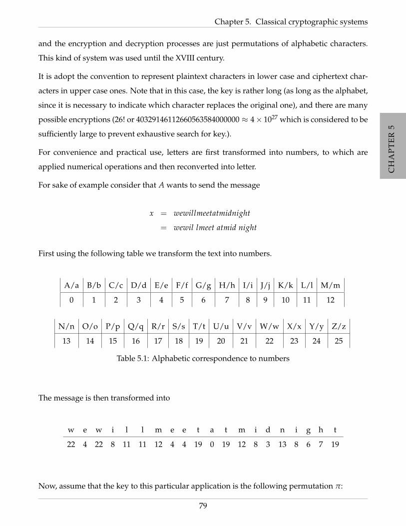
CH

AP

TE

R5

CH

AP

TE

R5

CH

AP

TE

R5

CH

AP

TE

R5


and the encryption and decryption processes are just permutations of alphabetic characters.

This kind of system was used until the XVIII century.

It is adopt the convention to represent plaintext characters in lower case and ciphertext char-

acters in upper case ones. Note that in this case, the key is rather long (as long as the alphabet,

since it is necessary to indicate which character replaces the original one), and there are many

possible encryptions (26! or 40329146112660563584000000 ≈ 4× 1027 which is considered to be

sufficiently large to prevent exhaustive search for key.).

For convenience and practical use, letters are first transformed into numbers, to which are

applied numerical operations and then reconverted into letter.

For sake of example consider that A wants to send the message

x = wewillmeetatmidnight

= wewil lmeet atmid night

First using the following table we transform the text into numbers.

A/a B/b C/c D/d E/e F/f G/g H/h I/i J/j K/k L/l M/m

0 1 2 3 4 5 6 7 8 9 10 11 12

N/n O/o P/p Q/q R/r S/s T/t U/u V/v W/w X/x Y/y Z/z

13 14 15 16 17 18 19 20 21 22 23 24 25

Table 5.1: Alphabetic correspondence to numbers

The message is then transformed into

w e w i l l m e e t a t m i d n i g h t

22 4 22 8 11 11 12 4 4 19 0 19 12 8 3 13 8 6 7 19

Now, assume that the key to this particular application is the following permutation π:

79

CH

AP

TE

R5

CH

AP

TE

R5

CH

AP

TE

R5

CH

AP

TE

R5


0 1 2 3 4 5 6 7 8 9 10 11 12

23 13 24 0 7 15 14 6 25 16 22 1 19

13 14 15 16 17 18 19 10 21 22 23 24 25

18 5 11 17 2 21 12 20 4 10 9 3 8

i.e., in terms of alphabet permutations, π is:

a b c d e f g h i j k l m

X N Y A H P O G Z Q W B T

n o p q r s t u v x w y z

S F L R C V M U E K J D I

Applying π to each letter of the message we transform the plaintext into:

w e w i l l m e e t a t m i d n i g h t

22 4 22 8 11 11 12 4 4 19 0 19 12 8 3 13 8 6 7 19

10 7 10 25 1 1 19 7 7 12 23 12 19 25 0 18 25 14 6 12

H P H T W W X P P E L E X T O Y T R S E

and the resulting ciphertext message is:

y = HPHTW WXPPE LEXTO YTRSE

= HPHTWWXPPELEXTOYTRSE

To decrypt the message B repeats this process but instead of using π uses is inverse π−1.

Summing up, a substitution cipher system can be formalized as follows:

Cryptographic system 5.1.3 (Substitution cipher system)

A substitution cipher system is a tuple S = (P, C, K, ek, dk) where:

1. P = C = Z26;

80

CH

AP

TE

R5

CH

AP

TE

R5

CH

AP

TE

R5

CH

AP

TE

R5


2. K consists of all possible permutations of the 26 symbols;

3. For each permutation π ∈ K, eπ(x) = π(x) and dπ(x) = π−1(x).

In the case that one want to use this type of encryption, it is not very convenient to use purely

random permutation since it is not very practical to decorate the permeation. So usually one

fixes a phrase without repetitions of letters to be the key. For example one can use the phrase:

”X-night try blew Jack Zvq of Drumps.”

Exercise 5.1.4. Show that the above cipher is in fact a cryptographic system.

Other examples of cryptographic systems are the shift ciphers (which a particular case with c =

3, for the letter C, is also known as Ceasar’s ciphers which was described in ”De Vita Caesarum,

Divus Iulius” , i.e, ”The Lives of the Caesars, The Deified Julius” , written in approximately 110

A.C) and the affine cipher which are presented in the next exercises.

Exercise 5.1.5 (shift or transposition cipher system).

Consider the following tuple T = (P, C, K, e, d) where:

1. P = C = K = Z26;

2. for all k ∈ K let ek(x) = (x + k) (mod 2)6 and dk(y) = (y− k) (mod 26).

Show that (P, C, K, e, d) is a cryptographic system.

Exercise 5.1.6 (affine cipher system). Consider the following tuple A = (P, C, K, e, d) where:

1. P = C = Z26;

2. K = Z∗26 ×Z26;

3. for all (k1; k2) ∈ K let e(k1,k2)(x) = (k1 · x + k2) (mod 26).

First, envisigate the need of the restriction to Z∗26 × Z26 of the keys. After, for each e(k1,k2) define the

respective deconding function d(k1,k2). Conclude by proving that the defined cipher system is, in fact, a

cryptographic system.

81

CH

AP

TE

R5

CH

AP

TE

R5

CH

AP

TE

R5

CH

AP

TE

R5


Exercise 5.1.7 (composition of shift cipher system). Let T = (Z26,Z26,Z26, e, d) and T ′ =

(Z26,Z26,Z26, e′, d′) be two shift cipher systems defined in Exercise 5.1.6. Show that they are equivalent

accordingly to Definition 5.1.2. Study the structure of a composition of any two of these systems.

• • •

5.1.3 The Verman cipher system

This cipher system was created and patented in 1917, by Gilbert Vernam and is also called

the one-time pad cryptographic system. It is one of the simplest cryptographic systems and is

described as follows:

The key is random, has the same length of the plaintext and it is used once justifying the

alternative name. It is a particular case of the substitution cipher that later on will be proved to

be perfectly secure.

Cryptographic system 5.1.8 (Verman cipher system)

The Verman cipher system also called the One time pad cipher system is the tuple O =

(P, C, K, e, d) such that:

1. P = C = K = 0, 1m;

2. For a key k = k1 · · · km ∈ K and for x = x1 · · · xm ∈ P and y = y1 · · · ym ∈ C, define

ek(x) = x⊕ k = x1 ⊕ k1 ⊕ xm ⊕ km

and

dk(y) = y⊕ k = y1 ⊕ k1 · · · ym ⊕ km

where the operation ⊕ is the exclusive OR defined by

⊕ 0 1

0 0 1

1 1 0

82

CH

AP

TE

R5

CH

AP

TE

R5

CH

AP

TE

R5

CH

AP

TE

R5


• • •

5.1.4 The Vigenere cipher

Although the cryptographic cipher system that is presented in the subsection ha the name of

Blaise de Vigenere, who lived in the sixteenth century, the authority of this kind of ciphers was

first reported by Giovan Battista Bellaso in his 1553 book La cifra del. Sig. Giovan Battista Bellaso.

The major difference between the substitution cipher and the Vigenere cipher is the fact that in

the latter one instead of encrypting character by character the massage to be sent, A encrypts

m alphabetic characters at a time by the use of a key of length m. For sake of presentation

consider for example that A wants to encrypt the message

x = attackatdawn

= attac katda wn

and A and B had chosen the key to be

k = LEMON

First using the Table 7.3 one gets:

a t t a c k a t d a w n

0 19 19 0 2 10 0 19 3 0 22 13

and

l e m o n

11 4 12 14 13

Now, organizing the numbers of the plaintext elements in groups of 5 elements, it is summed

each element of that group with the correspondent value of the key modulo 26, as follows:

83

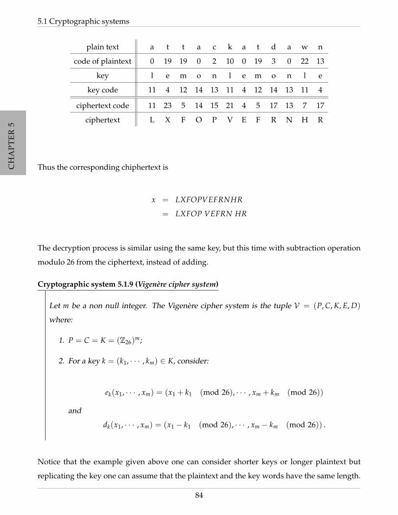
CH

AP

TE

R5

CH

AP

TE

R5

CH

AP

TE

R5

CH

AP

TE

R5


plain text a t t a c k a t d a w n

code of plaintext 0 19 19 0 2 10 0 19 3 0 22 13

key l e m o n l e m o n l e

key code 11 4 12 14 13 11 4 12 14 13 11 4

ciphertext code 11 23 5 14 15 21 4 5 17 13 7 17

ciphertext L X F O P V E F R N H R

Thus the corresponding chiphertext is

x = LXFOPVEFRNHR

= LXFOP VEFRN HR

The decryption process is similar using the same key, but this time with subtraction operation

modulo 26 from the ciphertext, instead of adding.

Cryptographic system 5.1.9 (Vigenere cipher system)

Let m be a non null integer. The Vigenere cipher system is the tuple V = (P, C, K, E, D)

where:

1. P = C = K = (Z26)m;

2. For a key k = (k1, · · · , km) ∈ K, consider:

ek(x1, · · · , xm) = (x1 + k1 (mod 26), · · · , xm + km (mod 26))

and

dk(x1, · · · , xm) = (x1 − k1 (mod 26), · · · , xm − km (mod 26)) .

Notice that the example given above one can consider shorter keys or longer plaintext but

replicating the key one can assume that the plaintext and the key words have the same length.

84

CH

AP

TE

R5

CH

AP

TE

R5

CH

AP

TE

R5

CH

AP

TE

R5


• • •

5.1.5 The Hill cipher

In this section, it is described the Hill cipher, another polyalphabetic cryptographic system

invented in 1929 by Lester Hill. The basic idea is to consider m linear combinations of the m

alphabetic characters in one plaintext element and works on groups of m letters at once and

thus the encryption can be achieved by matrix multiplication.

Cryptographic system 5.1.10 (Hill cipher system)

Let m ≥ 2 be a natural number. The Hill cipher system is the tuple (P, C, K, e, d) such that:

1. P = C = (Z26)m;

2. K = T : (Z26)m → (Z26)

m such that T is a linear isomorphism in (Z26)m;

3. For a key k ∈ K and for x ∈ P and y ∈ C, define

ek(x) = x · k

and

dk(x) = y · k−1.

Recall that T : (Z26)m → (Z26)

m is a linear isomorphism in (Z26)m if for all a ∈ Z and x, y ∈

(Z26)m, T(a · x + y) = aT(x) + T(y) and also if it is invertible.

Proposition 5.1.11. If T is a linear transformation in (Z26)m then there is a 26× 26 matrix M with

entries in (Z26)m such that T(x) = Mx for all x ∈ (Z26)

m.

Proof: The element Mi,j of M is equal to T(ei)j where ei is the vector of all zeros and 1 in the

position i.

Proposition 5.1.12. T is an isomorphism if and only if M is invertible.

The proof is direct and is left as an exercise.

85

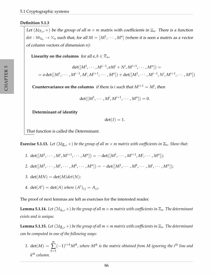
CH

AP

TE

R5

CH

AP

TE

R5

CH

AP

TE

R5

CH

AP

TE

R5


Definition 5.1.3

Let (MZn ,+) be the group of all m× m matrix with coefficients in Zn. There is a function

det : MZn → Zn such that, for all M = [M1, · · · , Mn] (where it is seen a matrix as a vector

of column vectors of dimension n):

Linearity on the columns for all a, b ∈ Zn,

det([M1, · · · , Mi−1, aMi + Ni, Mi+1, · · · , Mn]) =

= a det([M1, · · · , Mi−1, Mi, Mi+1, · · · , Mn]) + det([M1, · · · , Mi−1, Ni, Mi+1, · · · , Mn])

Countervariance on the columns if there is i such that Mi+1 = Mi, then

det([M1, · · · , Mi, Mi+1, · · · , Mn]) = 0.

Determinant of identity

det(I) = 1.

That function is called the Determinant.

Exercise 5.1.13. Let (MZn ,+) be the group of all m×m matrix with coefficients in Zn. Show that:

1. det([M1, · · · , Mi, Mi+1, · · · , Mn]) = −det([M1, · · · , Mi+1, Mi, · · · , Mn]);

2. det([M1, · · · , Mi, · · · , Mk, · · · , Mn]) = −det([M1, · · · , Mk, · · · , Mi, · · · , Mn]);

3. det(MN) = det(M)det(N);

4. det(At) = det(A) where (At)i,j = Aj,i.

The proof of next lemmas are left as exercises for the interested reader.

Lemma 5.1.14. Let (MZn ,+) be the group of all m×m matrix with coefficients inZn. The determinant

exists and is unique.

Lemma 5.1.15. Let (MZn ,+) be the group of all m×m matrix with coefficients inZn. The determinant

can be computed in one of the following ways:

1. det(M) =m

∑k=1

(−1)i+k Mik, where Mik is the matrix obtained from M ignoring the ith line and

kth column.

86

CH

AP

TE

R5

CH

AP

TE

R5

CH

AP

TE

R5

CH

AP

TE

R5


2. det(M) = ∑σ∈Sn

sign(σ)∏i=1

nMi,σi , where Sn is the set of all permutations σ over 1, · · · , n and

sign(σ) = (−1)N(σ) where N(σ) is the number of transposition in the decomposition of σ.

Theorem 5.1.1

Let (MZn ,+) be the group of all m×m matrix with coefficients in Zn. A matrix M ∈MZn is

invertible if and only if det(M) is an invertible number in Zn.

Proof:

(⇐) Simply observe that

1 = det(I) = det(MM−1) = det(M)det(M−1)

1 = det(I) = det(M−1M) = det(M−1)det(M).

This way, the inverse of det(M) is det(M−1).

(⇒)

Assume that M is a matrix and assume that det(M) = d where d ∈ Z26 is invertible. The matrix

N defined by Ni,j = d−1(−1)i+jdet(Mji) is the inverse of M.

In fact,

(MN)i,j =n

∑k=1

Mi,kNk,j = d−1n

∑k=1

Mi,k(−1)k+j det(Mjk)

In particular, if j = i

(MN)i,j = d−1n

∑k=1

Mi,k(−1)k+j det(Mjk) = d−1 · det(M) = d−1 · d = 1

and if j 6= i

(MN)i,j = d−1n

∑k=1

Mi,k(−1)k+j det(Mjk) = d−1 · 0 = 0.

87

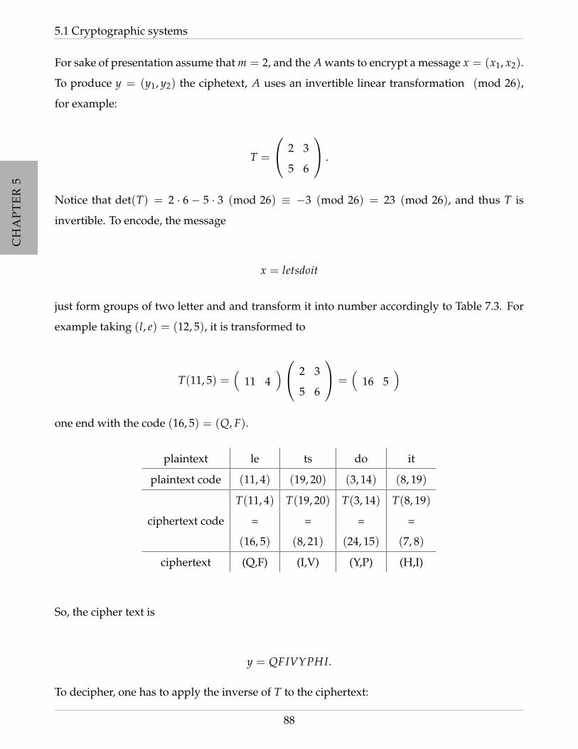
CH

AP

TE

R5

CH

AP

TE

R5

CH

AP

TE

R5

CH

AP

TE

R5


For sake of presentation assume that m = 2, and the A wants to encrypt a message x = (x1, x2).

To produce y = (y1, y2) the ciphetext, A uses an invertible linear transformation (mod 26),

for example:

T =

2 3

5 6

.

Notice that det(T) = 2 · 6 − 5 · 3 (mod 26) ≡ −3 (mod 26) = 23 (mod 26), and thus T is

invertible. To encode, the message

x = letsdoit

just form groups of two letter and and transform it into number accordingly to Table 7.3. For

example taking (l, e) = (12, 5), it is transformed to

T(11, 5) =(

11 4) 2 3

5 6

=(

16 5)

one end with the code (16, 5) = (Q, F).

plaintext le ts do it

plaintext code (11, 4) (19, 20) (3, 14) (8, 19)

T(11, 4) T(19, 20) T(3, 14) T(8, 19)

ciphertext code = = = =

(16, 5) (8, 21) (24, 15) (7, 8)

ciphertext (Q,F) (I,V) (Y,P) (H,I)

So, the cipher text is

y = QFIVYPHI.

To decipher, one has to apply the inverse of T to the ciphertext:

88

CH

AP

TE

R5

CH

AP

TE

R5

CH

AP

TE

R5

CH

AP

TE

R5


T−1 =

24 2

19 8

.

Theorem 5.1.2

Let (MZn ,+) be the group of all m × m matrix with coefficients in Zn and let M be an

invertible matrix in MZn . Then

M−1 = (det M)−1M∗

where M∗i,j = (−1)i+j det(Mij).

The proof of this result is left to the interested reader.

• • •

5.1.6 Stream ciphers

Until now all the cryptographic systems that were considered have the property that successive

plaintext elements are encrypted using the same key and are also memoryless, in the sense that

the same function is used to encrypt successive blocks and there is no need to use previous

computed information to encrypt other elements. This means that in this kind of systems to

encrypt, for example the second element the system will use some informations computed to

the first element encrypted.

Another approach possible to design cryptographic schemes is to use what are called stream

ciphers where individual characters, one at a time, are encrypted, with a cipher that varies with

time and have memory since there are state functions that record the state of the function to

be used in later stages. An example of this type of cryptographic system, called synchronous

is one that constructs a keystream, i.e., a sequence of characters generated from the key and

the state of the function, as input to the stream cipher and independently from the plaintext

message and is presented bellow. Another example, called self-synchronizing or asynchronous

stream cipher is a stream cipher in which the keystream is a function of the key and a fixed

number of previous ciphertext characters.

89

CH

AP

TE

R5

CH

AP

TE

R5

CH

AP

TE

R5

CH

AP

TE

R5


Cryptographic system 5.1.16 (synchronous stream cipher)

A tupe (P, C, K, L, e, d) together with a function g is said to be a synchronous stream cipher

if the following properties hold:

1. P is the finite set of all possible plaintexts;

2. C is the finite set of all possible ciphertexts;

3. K is the finite set of possible keys;

4. L is a finite set called the keystream alphabet;

5. g is the keystream generator, i.e., g takes a key k ∈ K as input, and generates an infinite

string z1z2 · · · called the keystream, such that for all i > 1, zi ∈ L.

6. For each z ∈ L, there is an encryption function ez : P → C and a decryption function

dz : C → P such that for all x ∈ P, dz(ez(x)) = x.

A stream cipher is a periodic stream cipher with period d if zi+d = zi for all integers i > 1. The

Vigenere Cipher with keyword length m,is a periodic stream cipher with period m since it can

be define using the keystream

zi =

ki if 1 ≤ i ≤ m

zi−m if otherwise,

where k = (k1, · · · , km) is the key of the Vigenere cipher.

• • •

5.1.6.1 Linear Feedback Shift Registers

A linear feedback shift register (LFSR) is a shift register whose input bit is a linear function of

its previous state and hence is an elementary algorithm to generate a keystream, that among

other properties, is able to produce sequences with large periods and is easy to implement in a

computer.

In general, one can define a LFSR from the algorithmic point of view, using an n staged

90

CH

AP

TE

R5

CH

AP

TE

R5

CH

AP

TE

R5

CH

AP

TE

R5


algorithm, where each stage Rn−1, · · · , R1, R0, store one bit, with one input and one output,

and a timer which marks the evolution of the stages such that on the ith cycle:

1. the contents of stage 0 is “output”

2. the contents of Ri moves to Ri−1, for 1 ≤ i ≤ n− 1 and

3. the content of stage Rn−1 is a bynary linear combination of all the contents of the earlier

stages 0, 1, . . . , n− 2.

If one denotes the contents of stage Rj on cycle i by si+j, this allows to describe the stage Rn−1

in terms of a recurrence relationship

sn+i =n−1

∑j=0

cn−jsi+j,

where cj, 1 ≤ j ≤ n are some constants 0 or 1 specifying the stages which contribute to the

sum.

It is common to identify the constants ck as coefficients of a polynomial

g(x) =n

∑k=0

ckxk,

called connection polynomial of the LFSR.

For sake of understanding the LFSR it is presented next an example of this type of crypto-

graphic cipher system to generate a synchronous keystream.

Example 5.1.17. Start with a binary m-tuple (k1, · · · , km) and define for all 1 ≤ i ≤ m, zi = ki. The

subsequent keystream is defined using a linear recurrence of degree m (i.e., each term depends on the

previous m terms):

zi+m =m−1

∑j=0

cjzi+j (mod 2).

So the key Here is k = k0, · · · , km−1, c0, ..., cm1. Notice that if all ki = 0 then the keystream is just all

0’s leading to a ciphertext equal to the plaintext. The trick is to choose the constants c0, · · · , cm1 cleverly

to produce a periodic keystream with period 2m− 1.

An example of non-synchronous stream cipher is the Autokey Cipher where the plaintext is

used to construct the keystream with the initial priming key k.

91

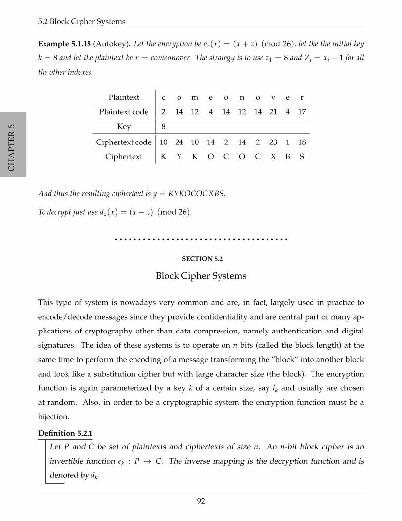
CH

AP

TE

R5

CH

AP

TE

R5

CH

AP

TE

R5

CH

AP

TE

R5

5.2 Block Cipher Systems

Example 5.1.18 (Autokey). Let the encryption be ez(x) = (x + z) (mod 26), let the the initial key

k = 8 and let the plaintext be x = comeonover. The strategy is to use z1 = 8 and Zi = xi − 1 for all

the other indexes.

Plaintext c o m e o n o v e r

Plaintext code 2 14 12 4 14 12 14 21 4 17

Key 8

Ciphertext code 10 24 10 14 2 14 2 23 1 18

Ciphertext K Y K O C O C X B S

And thus the resulting ciphertext is y = KYKOCOCXBS.

To decrypt just use dz(x) = (x− z) (mod 26).

• • • • • • • • • • • • • • • • • • • • • • • • • • • • • • • • • • • • •

SECTION 5.2

Block Cipher Systems

This type of system is nowadays very common and are, in fact, largely used in practice to

encode/decode messages since they provide confidentiality and are central part of many ap-

plications of cryptography other than data compression, namely authentication and digital

signatures. The idea of these systems is to operate on n bits (called the block length) at the

same time to perform the encoding of a message transforming the ”block” into another block

and look like a substitution cipher but with large character size (the block). The encryption

function is again parameterized by a key k of a certain size, say lk and usually are chosen

at random. Also, in order to be a cryptographic system the encryption function must be a

bijection.

Definition 5.2.1

Let P and C be set of plaintexts and ciphertexts of size n. An n-bit block cipher is an

invertible function ek : P → C. The inverse mapping is the decryption function and is

denoted by dk.

92

CH

AP

TE

R5

CH

AP

TE

R5

CH

AP

TE

R5

CH

AP

TE

R5


The idea, similar to what happens in the previous example, if the plaintext messages exceeds

one block in length then several techniques are applied to operate all the blocks individually.

One can evaluate the block ciphers with respect to the estimated security level (based on the

general use by the community), the key size (that defines upper bound on the security but

longer keys require, in general, more resources, memory, processing time, etc), the efficiency of

the process, the block size (that affects the complexity of the system and its security), etc.

Recall that when a message has more than n bits, one can, for example, divide the message

into n-bit blocks and encrypt each separately enabling the repetition and secure use of a block

cipher under a single key. In what follows, it is described the 4 basic modes of operation of a

block cipher system to address the encryption of several block. The four most common modes

are ECB, CBC, CFB, and OFB. These are the first modes of operation and were proposed and

specified in FIPS 81 in 1981.

• • •

5.2.1 ECB mode

The nomenclature ECB means electronic codebook and is the mode of operation where each

block is ciphered using the same key, like the Vigenere cipher system. As it will be seen in the

next section this type of encryption in vulnerable to attack that exploit statistical properties of

the texts. Notice that identical blocks of plaintext are encrypted into identical ciphertext which

means that is does not hide patterns.

Algorithm 5.2.1 (ECB mode)

Input: A lk bit string k as a key and x1, · · · , xt blocks of plaintexts of a certain length

Output: y1, · · · , yt blocks of ciphertexts;

Step 1: i = 0;

Step 2: While i ≤ t do

Step 2.1: yi = ek(xi);

Step 2.2: i = i + 1;

Step : Output y = y1 · · · yt;

93

CH

AP

TE

R5

CH

AP

TE

R5

CH

AP

TE

R5

CH

AP

TE

R5


The decoding method is clear and consists basically by replacing the use of ek by the use of dk.

• • •

5.2.2 CBC mode

The nomenclature CBC means cipher block chaining and is the mode of operation where

each block is ciphered using the same key but at each block the plaintext ins mixed with

the previous one. Notice that identical blocks of plaintext are only encrypted into identical

ciphertext whenever the same part of the initial plain text and the same part of the key is used.

94

CH

AP

TE

R5

CH

AP

TE

R5

CH

AP

TE

R5

CH

AP

TE

R5


Notice also that since to encrypt a part of the plaintext one needs part of the previous block then

the entire system is dependent on each other and the chaining mechanism causes ciphertext to

be completely different and thus the decryption process cannot be executed separately like in

the previous case.

Algorithm 5.2.2 (CBC mode - encryption)

Input: A lk bit string k as a key, x1, · · · , xt blocks of plaintexts of a certain length and an

initial block x0 of the same size of the others.

Output: y0y1, · · · , yt blocks of ciphertexts;

Step 1: y0 = x0;

Step 2: i = 1;

Step 3: While i ≤ t do

Step 3.1: yi = ek(yi−1 ⊕ xi);

Step 3.2: i = i + 1;

Step 4: Output y = y0 · · · yt;

95

CH

AP

TE

R5

CH

AP

TE

R5

CH

AP

TE

R5

CH

AP

TE

R5


The decoding method is:

Algorithm 5.2.3 (CBC mode- decryption)

Input: A lk bit string k as a key, y1, · · · , yt blocks of ciphertexts of a certain length.

Output: x1, · · · , xt blocks of plaintexts;

Step 2: i = t;

Step 3: While i ≥ 0 do

Step 3.1: xi = yi−1 ⊕ dk(yi);

Step 3.2: i = i− 1;

Step 4: Output x = x1 · · · xt;

• • •

5.2.3 CFB mode

The nomenclature CFB means cipher feedback and is closely related with the CBC mode, which

makes a block cipher into a self-synchronizing stream cipher. It is assume that a shift register

is available as described in the previous section.

96

CH

AP

TE

R5

CH

AP

TE

R5

CH

AP

TE

R5

CH

AP

TE

R5


Algorithm 5.2.4 (CFB mode - encryption)

Input: A lk bit string k as a key, x1, · · · , xu blocks of plaintexts of length r and an initial

value for a shift register of length n > r called x0.


Step 1: I1 = x0;

Step 2: i = 1;

Step 3: While i ≤ u do

Step 3.1: Oi = ek(Ii);

Step 3.2: ti = the r leftmost bits of Oi;

Step 3.3: yi = xi ⊕ ti;

Step 3.4: Ii+1 = 2r Ii + yi (mod 2n)

Step 4: Output y = y1 · · · yu;

97

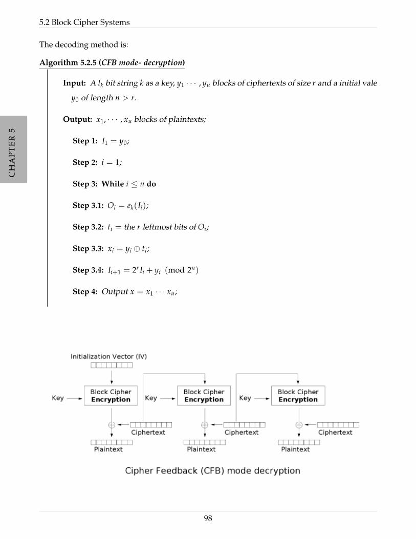
CH

AP

TE

R5

CH

AP

TE

R5

CH

AP

TE

R5

CH

AP

TE

R5



Algorithm 5.2.5 (CFB mode- decryption)

Input: A lk bit string k as a key, y1 · · · , yu blocks of ciphertexts of size r and a initial vale

y0 of length n > r.

Output: x1, · · · , xu blocks of plaintexts;

Step 1: I1 = y0;

Step 2: i = 1;




Step 3.3: xi = yi ⊕ ti;

Step 3.4: Ii+1 = 2r Ii + yi (mod 2n)

Step 4: Output x = x1 · · · xu;

98

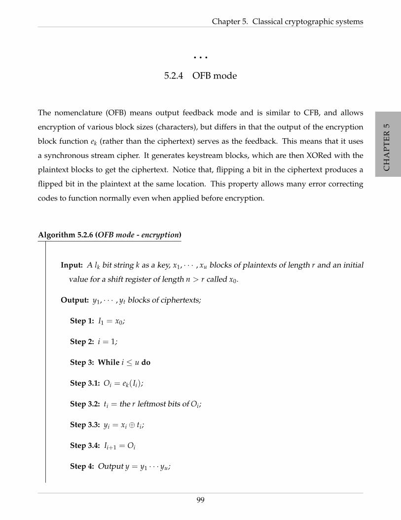
CH

AP

TE

R5

CH

AP

TE

R5

CH

AP

TE

R5

CH

AP

TE

R5


• • •

5.2.4 OFB mode

The nomenclature (OFB) means output feedback mode and is similar to CFB, and allows

encryption of various block sizes (characters), but differs in that the output of the encryption

block function ek (rather than the ciphertext) serves as the feedback. This means that it uses

a synchronous stream cipher. It generates keystream blocks, which are then XORed with the

plaintext blocks to get the ciphertext. Notice that, flipping a bit in the ciphertext produces a

flipped bit in the plaintext at the same location. This property allows many error correcting

codes to function normally even when applied before encryption.

Algorithm 5.2.6 (OFB mode - encryption)

Input: A lk bit string k as a key, x1, · · · , xu blocks of plaintexts of length r and an initial

value for a shift register of length n > r called x0.


Step 1: I1 = x0;

Step 2: i = 1;




Step 3.3: yi = xi ⊕ ti;

Step 3.4: Ii+1 = Oi

Step 4: Output y = y1 · · · yu;

99

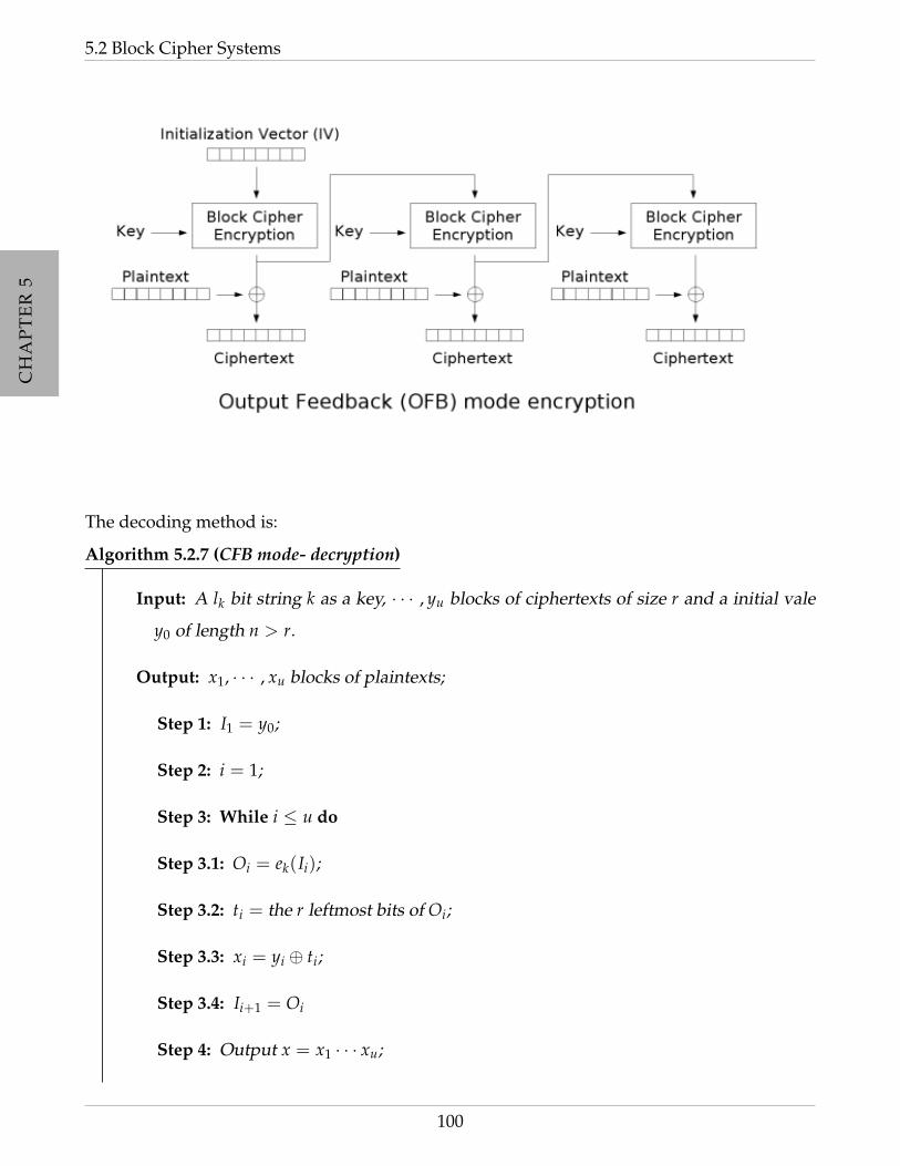
CH

AP

TE

R5

CH

AP

TE

R5

CH

AP

TE

R5

CH

AP

TE

R5



Algorithm 5.2.7 (CFB mode- decryption)

Input: A lk bit string k as a key, · · · , yu blocks of ciphertexts of size r and a initial vale

y0 of length n > r.

Output: x1, · · · , xu blocks of plaintexts;

Step 1: I1 = y0;

Step 2: i = 1;




Step 3.3: xi = yi ⊕ ti;

Step 3.4: Ii+1 = Oi

Step 4: Output x = x1 · · · xu;

100

CH

AP

TE

R5

CH

AP

TE

R5

CH

AP

TE

R5

CH

AP

TE

R5


• • • • • • • • • • • • • • • • • • • • • • • • • • • • • • • • • • • • •

SECTION 5.3

Breaking down the cryptographic system

Since someone hd the need of ”hiding” information there is always someone on the other side

trying to break it down without the authorization and the consent of the rightful parties. There

are several types of attacks that an opponent can preform to access the secret information.

Before explaining the techniques there some comments have to me made. The first one is

related with the following statement:

The security of a cipher text should not be based on the assumption that an oppo-

nent does not which cipher A and B were using.

In fact, if one bases the security of “hiding” secret information on the fact that the adversaries

do not know a priori the cipher system since it can try in parallel several attacks presuming, at

each time, that the system is one of the known systems. Also, rather that putting all the eggs in

the same basket, it is better to ensure security by the design presuming that it “secure” rather

than using some techniques of encrypting that are known to be insecure and by obscurity.

101

CH

AP

TE

R5

CH

AP

TE

R5

CH

AP

TE

R5

CH

AP

TE

R5

5.3 Breaking down the cryptographic system

This principle is known as the “Kerckhoffs’ principle”. From the point of view of A and B they

rather have a system that is secure even if someone else knowing the type of encryption that

was used, than risk the hypothesis of their secret message being discovered by trial and error.

The name of the principle is due to Auguste Kerckhoffs that in the19th century,published his

opinion about the security of a cryptographic system outlining important design principles of

such systems.

The cipher method must not be required to be secret, and it must be able to fall into

the hands of the enemy without inconvenience. A cryptographic system should

be secure even if everything about the system, except the key, is public knowledge.

Auguste Kerckhoffs

Stated differently, Kerckhoffs’ principle only requires that security rely only on the secrecy of

the key, which seems dangerous. Although, one can argue in favor of this principle. First,

for convenience, is that it is much easier for A and B to keep secret only a short key rather

than keeping secret all the encryption/decryption method, since the first one is a string of

some bits or bits and store this string securely, and the latter case also one needs to share and

securely store the entire scheme that is thousands of times larger. Also, it might happen that

details of scheme can be leaked (perhaps by an insider) or learned through reverse engineering.

This situation is very improvable in the case of the secret key is a randomly generated string.

Another point in favor to Kerckhoffs’ principle is that in case the key is exposed, it is simpler

to A and B agree to use another key that to replace the algorithm that is being-used. In terms

of practically of use, in case many pairs of people, for example in a company, that encrypt

their communication, one can imagine to be easier for all parties to use the same scheme, but

different keys, than for everyone to use a different schemes. A discussion about the practically

of shared string will be done in due course.

Nowadays, Kerckhoffs’ principle is interpreted with the sense that security can not depend on

secrecy of the scheme and, in fact, they should be public in contrast to the notion of ”security

by obscurity ” which is the idea that improved security can be achieved by keeping a cryp-

tographic algorithm hidden. Notice that being public enables the establishment of standards

102

CH

AP

TE

R5

CH

AP

TE

R5

CH

AP

TE

R5

CH

AP

TE

R5


used worldwide and also, such designs have been widely studied and for that reason one can

easily believe that it is stronger.

The different possible attack models on cryptographic systems can be specified in terms of the

information available to the adversary when he mounts his attack and can be:

Ciphertext only attack: the cryptanalyst has access only to a collection of ciphertexts or

codetexts. This type of attack is also known as Eavesdropping.

Known plaintext attack: the attacker has access to some ciphertexts with the corres-

ponding plaintext, which might result from, for example, a temporary access to the en-

cryption method so it can choose a plaintext string and construct the corresponding

encryption. It might also result from some informations that the attacker might know

to be present in certain parts of the ciphertext.

Chosen plaintext (resp. ciphertext) attack: the opponent has access to some plaintexts

(resp. ciphertext) corresponding to an arbitrary set of plaintexts (resp. ciphertext) of his

own choice. Notice that in the case of ciphertext attacks, if the opponent only wants to

know the corresponding plaintext he can get it without any effort, but in the ultimate

case, he wants to be able to decrypt anything. So the idea is to gain knowledge not only

about the text but also about the decryption process (namely the key).

Adaptive chosen plaintext (resp. ciphertext) attacks: This type of attacks are similar to

the chosen plaintext (resp. ciphertext) attacks, but in this particular type the attacker

can choose subsequent plaintexts (resp. ciphertext) based on information learned from

previous encryptions (resp. decryptions).

Physical modification of messages: In this type of attacks the opponent forges some

messages trying to convince the parties to be a legal message.

In all these cases, the goal of the opponent is to determine the ”key” that is used, allowing the

decryption not only a specific ciphertext but also the decryption of any ciphertext encrypted

using the same key.

The most basic attack is the cipher text only attack and it is normally the only information that

an opponent has access to. In the sequel it is assumed that the plaintext is written in English,

103

CH

AP

TE

R5

CH

AP

TE

R5

CH

AP

TE

R5

CH

AP

TE

R5


without punctuation or ”spaces”. The reader is invited to think why that if punctuations and

spaces where allowed the breaking process would become easier.

The main technique for breaking the ciphers is the statistic analysis. Each language, and in

particular the English one, has a unique statistical signature. It is well known that letters in

a natural language have stable frequencies and the knowledge of this frequency distribution

provides a clue for cryptanalysis.

In fact, the frequency of each letter, the frequency of each digrams and other combination of

letters and the frequency of certain words in common texts can be seen as “fingerprint” of the

language and it can be used to cryptographic analyze cipher texts.

Several studies of this statistical properties have been done and they conclude that, for ex-

ample, the letter E is the most frequent one, the digram TH is the most common and the

combination ING appears quite a lot.

In the next figure and table it is summarized the frequency of each letter:

Figure 5.1: English letter frequencies, sorted by frequency and alphabetic, from Wikipedia

104

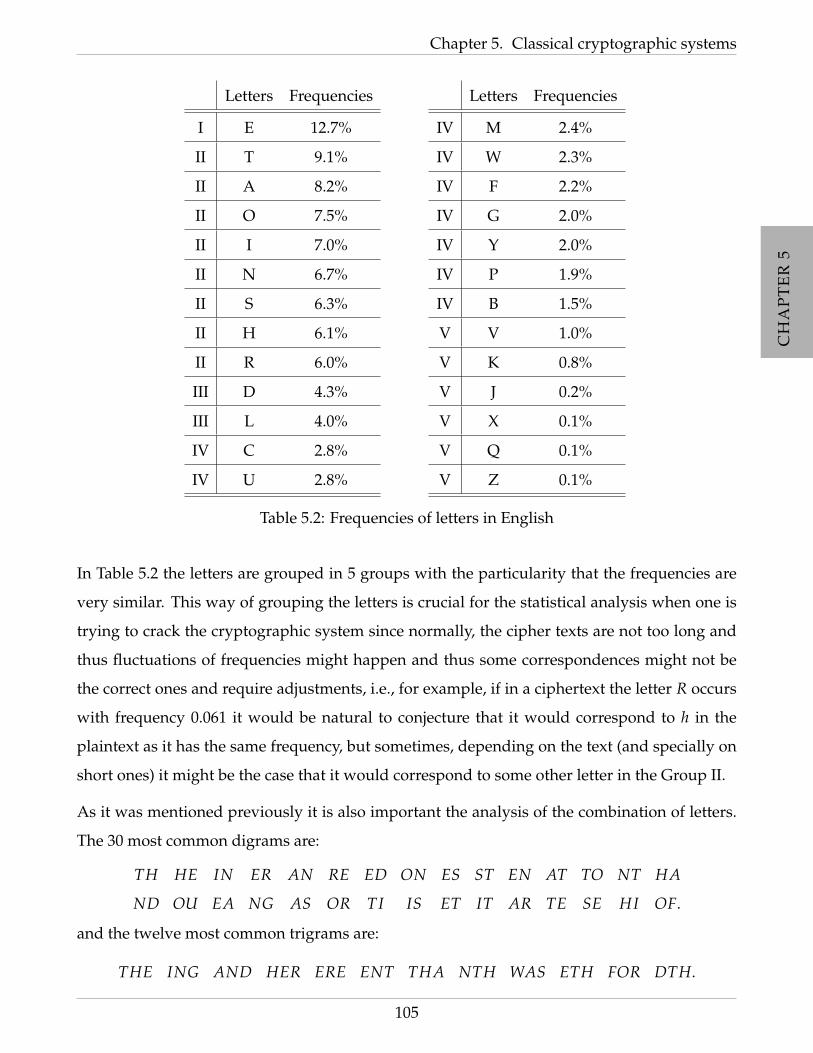
CH

AP

TE

R5

CH

AP

TE

R5

CH

AP

TE

R5

CH

AP

TE

R5


Letters Frequencies

I E 12.7%

II T 9.1%

II A 8.2%

II O 7.5%

II I 7.0%

II N 6.7%

II S 6.3%

II H 6.1%

II R 6.0%

III D 4.3%

III L 4.0%

IV C 2.8%

IV U 2.8%

Letters Frequencies

IV M 2.4%

IV W 2.3%

IV F 2.2%

IV G 2.0%

IV Y 2.0%

IV P 1.9%

IV B 1.5%

V V 1.0%

V K 0.8%

V J 0.2%

V X 0.1%

V Q 0.1%

V Z 0.1%

Table 5.2: Frequencies of letters in English

In Table 5.2 the letters are grouped in 5 groups with the particularity that the frequencies are

very similar. This way of grouping the letters is crucial for the statistical analysis when one is

trying to crack the cryptographic system since normally, the cipher texts are not too long and

thus fluctuations of frequencies might happen and thus some correspondences might not be

the correct ones and require adjustments, i.e., for example, if in a ciphertext the letter R occurs

with frequency 0.061 it would be natural to conjecture that it would correspond to h in the

plaintext as it has the same frequency, but sometimes, depending on the text (and specially on

short ones) it might be the case that it would correspond to some other letter in the Group II.

As it was mentioned previously it is also important the analysis of the combination of letters.

The 30 most common digrams are:

TH HE IN ER AN RE ED ON ES ST EN AT TO NT HA

ND OU EA NG AS OR TI IS ET IT AR TE SE HI OF.

and the twelve most common trigrams are:

THE ING AND HER ERE ENT THA NTH WAS ETH FOR DTH.

105

CH

AP

TE

R5

CH

AP

TE

R5

CH

AP

TE

R5

CH

AP

TE

R5


• • •

5.3.1 Breaking down the substitution cipher

Recall that in the substitution cipher system each letter is replaced by another one according

to a permutation. This kind of system has the property of preserving the properties of fre-

quency of the permuted letter allowing the opponent to do a statistical analysis and infer the

permutation used.

Assume that the following ciphertext is given

JWWEJ TYNUM FDFYJ TYJVU TQFVE FFCSE VURVF TNFJO FTHEU QUOZU NFYVE

FQRFH NZRJT SVUVE FCRRF NZFQV CXFNV JVCUT NJVVE FNZJT AFRMR JCWNJ

TYUKV EJKWV UZNJC WNEFF VNJTY EJWDJ RYNVE FPCMY UHTEJ KWJTY VEFVU

ZNJCW QWFHW CTFNJ TYMKT VWCTF NVEFD UKTSN JCWUR SJXFJ WUUAV UNFFV

EJVEC NURYF RNHFR FZRUO ZVWDJ TYJQQ KRJVF WDUMF DFYJT YVEFT VKRTF

YJSJC TVUVE FUHTF R

and one wants to decode the “secret” message hidden.

Notice that the text has 291 characters. The first step is to count the characters and perform a

statistical analysis:

F J V T U N E R Y W C Z

38 30 29 23 22 20 18 16 15 15 13 8

13.4% 10.3% 9.9% 7.9% 7.6% 6.8% 6.2% 5.5% 5.2% 5.2% 4.5% 2, 7%

K Q D H M S O X A P L B I G

7 7 6 6 5 5 3 2 2 1 0 0 0 0

2.4% 2.4% 2.1% 2.1% 1.7% 1.7% 1.0% 0.7% 0.7% 0.3% 0% 0% 0% 0%

Since F occurs more frequently than others it is reasonable to conjecture that d(F) = e.

The other 8 most frequent characters that happen in the text are J, V, T, U, N, E, R, Y and for

the same reason it is reasonable to expect that these letters are encryptions of (a subset of) t, a,

106

CH

AP

TE

R5

CH

AP

TE

R5

CH

AP

TE

R5

CH

AP

TE

R5


o, i, n, s, h, r, but the frequencies really do not vary enough to tell us what the correspondence

might be. The digram EF occurs 10 times, the trigram VEF occurs 9 times and FE does not

occur it is reasonable to assume d(E) = h and d(V) = t. Also FT occurs 3 times and FTN

occurs once one may assume that d(T) = n and D(Y) = d. A similar argument can be used to

conjecture that d(R) = r and d(U) = o since “er” and “to” are also common digrams.

Since ”an” is also a common digram one may guess that d(J) = a.


a--ha nd-o- e-eda ndato n-eth ee--- torte n-ea- en--o -o--o -edth


e-re- --ran -toth e-rre --e-t --e-t at-on -atth e--an -er-r a---a


ndo-t ha--t o--a- --hee t-and h---a rd-th e---d o-nha --and the-o


--a-- --e-- -ne-a nd--n t--ne -the- o-n-- a--or -a-ea -oo-- o-eet


hath- -orde r--er e-ro- -t--a nda-- -rate --o-e -edan dthen t-rne

YJSJC TVUVE FUHTF R

d--a- ntoth eo-ne r

If the guesses are right and since aWW is followed by two equal letter one may conjuncture

that d(W) = l. Since “se”, “es” and “st” are common digrams and “NF”, “FN” and “NV”

appear also in the chiphertext it is reasonable to assume that d(N) = s, leading to:


allha ndso- e-eda ndato n-eth ee--- torte nsea- en--o -o--o sedth

107

CH

AP

TE

R5

CH

AP

TE

R5

CH

AP

TE

R5

CH

AP

TE

R5



e-re- s-ran -toth e-rre s-e-t --est at-on satth es-an -er-r a-lsa


ndo-t ha-lt o-sa- lshee tsand h-l-a rdsth e---d o-nha -land the-o


-sa-l -le-l -nesa nd--n tl-ne sthe- o-n-s a-lor -a-ea loo-- oseet


hath- sorde rs-er e-ro- -tl-a nda-- -rate l-o-e -edan dthen t-rne

YJSJC TVUVE FUHTF R

d--a- ntoth eo-ne r

Now one can infer the code of the rest of the consonants. For example, stat − on which is

encoded by NV JVCUT suggests that d(C) = i. Similarly, VKRTFY which is t− rned decoded

suggests that d(K) = u.


allha ndso- e-eda ndato n-eth eei-- torte nsea- en--o -o--o sedth


e-re- s-ran -toth eirre s-e-t i-est ation satth es-an -er-r ailsa


ndout hault o-sai lshee tsand h-l-a rdsth e-i-d o-nha uland the-o


-sail -le-l inesa nd-un tline sthe- oun-s ailor -a-ea loo-- oseet

108

CH

AP

TE

R5

CH

AP

TE

R5

CH

AP

TE

R5

CH

AP

TE

R5



hathi sorde rs-er e-ro- -tl-a nda-- urate l-o-e -edan dthen turne

YJSJC TVUVE FUHTF R

d--ai ntoth eo-ne r

Now for example one could infer that d(M) = f has for example the word “of” is common.

But in the text one would get words like “frails” which is a non sense. Using similar reasoning

it is now easy to decode the rest of the text to get:

all hands obeyed and at once the eight or ten seamen who composed the crew

sprang to their respective stations at the spanker brails and outhaul topsail sheets

and halyards the jib downhaul and the topsail clewlines and buntlines the young

sailor gave a look to see that his orders were promptly and accurately obeyed and

then turned again to the owner

“The count of Monte Cristo”

Alexandre Dumas.

Exercise 5.3.1. Envisigate on a possible attack to a shift cipher system and affine cipher system presented

in Exercises 5.1.5 and 5.1.6 respectively.

The reader might not find any difficulty breaking down a Ceasar chipper of any size and in

particular the smallest one since there are only a few keys that one can use to encrypt. The

same issue happens for the substitution ciphers (specially if one uses the computer for a brute

force attack). The vulnerability is the number of possible keys available.

This consideration leads to what it is called the ”sufficient key space principle”:

Any secure encryption scheme must have a key space that is not vulnerable to exhaustive

search.

109

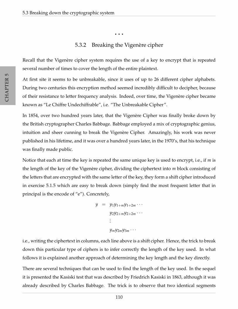
CH

AP

TE

R5

CH

AP

TE

R5

CH

AP

TE

R5

CH

AP

TE

R5


• • •

5.3.2 Breaking the Vigenere cipher

Recall that the Vigenere cipher system requires the use of a key to encrypt that is repeated

several number of times to cover the length of the entire plaintext.

At first site it seems to be unbreakable, since it uses of up to 26 different cipher alphabets.

During two centuries this encryption method seemed incredibly difficult to decipher, because

of their resistance to letter frequency analysis. Indeed, over time, the Vigenere cipher became

known as “Le Chiffre Undechiffrable”, i.e. “The Unbreakable Cipher”.

In 1854, over two hundred years later, that the Vigenere Cipher was finally broke down by

the British cryptographer Charles Babbage. Babbage employed a mix of cryptographic genius,

intuition and sheer cunning to break the Vigenere Cipher. Amazingly, his work was never

published in his lifetime, and it was over a hundred years later, in the 1970’s, that his technique

was finally made public.

Notice that each at time the key is repeated the same unique key is used to encrypt, i.e., if m is

the length of the key of the Vigenere cipher, dividing the ciphertext into m block consisting of

the letters that are encrypted with the same letter of the key, they form a shift cipher introduced

in exercise 5.1.5 which are easy to break down (simply find the most frequent letter that in

principal is the encode of “e”). Concretely,

y = y1y1+my1+2m · · ·

y2y2+my2+2m · · ·...

ymy2my3m · · ·

i.e., writing the ciphertext in columns, each line above is a shift cipher. Hence, the trick to break

down this particular type of ciphers is to infer correctly the length of the key used. In what

follows it is explained another approach of determining the key length and the key directly.

There are several techniques that can be used to find the length of the key used. In the sequel

it is presented the Kasiski test that was described by Friedrich Kasiski in 1863, although it was

already described by Charles Babbage. The trick is to observe that two identical segments

110

CH

AP

TE

R5

CH

AP

TE

R5

CH

AP

TE

R5

CH

AP

TE

R5


of plaintext will be encrypted to the same ciphertext whenever their occurrence are δ positions

apart from each other, where δ is such that δ ≡ 0 (mod m). On the other hand, if two segments

of ciphertext (of length at least 3) is observed, then the probability that they correspond to

identical segments of plaintext is high and can be used to infer the factors of the length of the

key. The Kasiski test can be described in the following way: First one searches the ciphertext

for pairs of identical segments of length at least 3, and write down the respective distances

between the starting positions of the segments. In fact, if several of such distances occur, then

one may infer that, probably, the length of the key is a divisor of the greatest common divisor

of all those distances.

Example 5.3.2. Assume that an opponent intersects the following block of ciphertext from a communi-

cation between A and B that was ciphered with a Vigenere cipher.

ISETI LLSUS BFCJX DCECH UZRQR TEHKR VLNFW DXUEL UTNGL TLLVL IZBGT JWLGH

SZWPS JEOHX WPYQY CRBTI PEHIM KTNIE XCIDS JRHVE SZZGR KZLWQ TDOPF PYKKR

VLNFG GPDKX PYDKR KPSVQ TYTUI RFRKX XPSCR SEHGC HEOQH DYMAW WPLHM CCEFE

COGQP SWIMI CPWOS CPYHV DXTJI BTNVT GZMKW XYGVS JYFQP SEHGW WTNKR VDEEV

TESVL PEOPP NXIFE HLNFQ DCGCR PYDOE TNEPE HVNGA

The trigrams “KRV” and “LNF” occur 3 times each in the ciphertext on the positions 32, 122 and 257

and 29, 119 and 234 leading to the distances 90, 115 and 135 which have 5 as greatest common divisor.

So, with high probability, 5 in the length of the key.

The index of coincidence is another useful tool that one can use to crack the Vigenere cipher.

This tool was proposed and studied by William Friedman in 1920, as follows.

Definition 5.3.1 (Index of coincidence)

Let x = x1x2 · · · xn be a string of n alphabetic characters. The index of coincidence of

x, denoted by Ic(x) is defined to be the probability that two random elements of x are

identical. If f0, · · · f25 are the frequencies of the letter of the alphabet in x then

Ic(x) =

25

∑i=0

(fi

2

)(

n2

) =25

∑i=0

fi( fi − 1)n(n− 1)

.

111

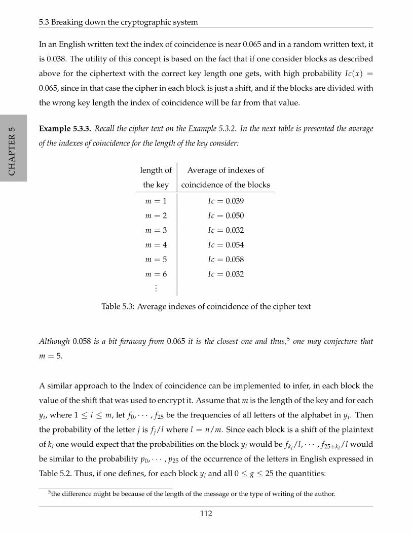
CH

AP

TE

R5

CH

AP

TE

R5

CH

AP

TE

R5

CH

AP

TE

R5


In an English written text the index of coincidence is near 0.065 and in a random written text, it

is 0.038. The utility of this concept is based on the fact that if one consider blocks as described

above for the ciphertext with the correct key length one gets, with high probability Ic(x) =

0.065, since in that case the cipher in each block is just a shift, and if the blocks are divided with

the wrong key length the index of coincidence will be far from that value.

Example 5.3.3. Recall the cipher text on the Example 5.3.2. In the next table is presented the average

of the indexes of coincidence for the length of the key consider:

length of Average of indexes of

the key coincidence of the blocks

m = 1 Ic = 0.039

m = 2 Ic = 0.050

m = 3 Ic = 0.032

m = 4 Ic = 0.054

m = 5 Ic = 0.058

m = 6 Ic = 0.032...

Table 5.3: Average indexes of coincidence of the cipher text

Although 0.058 is a bit faraway from 0.065 it is the closest one and thus,5 one may conjecture that

m = 5.

A similar approach to the Index of coincidence can be implemented to infer, in each block the

value of the shift that was used to encrypt it. Assume that m is the length of the key and for each

yi, where 1 ≤ i ≤ m, let f0, · · · , f25 be the frequencies of all letters of the alphabet in yi. Then

the probability of the letter j is f j/l where l = n/m. Since each block is a shift of the plaintext

of ki one would expect that the probabilities on the block yi would be fki /l, · · · , f25+ki /l would

be similar to the probability p0, · · · , p25 of the occurrence of the letters in English expressed in

Table 5.2. Thus, if one defines, for each block yi and all 0 ≤ g ≤ 25 the quantities:

5the difference might be because of the length of the message or the type of writing of the author.

112

CH

AP

TE

R5

CH

AP

TE

R5

CH

AP

TE

R5

CH

AP

TE

R5


Myi,g =25

∑i=0

pi · fi+g

l

one expects to get Myi,g ≈ 0.065 if g = ki and Myi,g 6≈ 0.065 if g 6= ki.

Example 5.3.4. Continuing the Example 5.3.2, and producing the calculus for all of the 5 blocks one

would conclude that the key used was K = (15, 11, 0, 2, 4) leading to the key K = place and to the

plaintext:

there was so much to read for one thing and so much fine health to be pulled

down out of the young breath giving air i bought a dozen volumes on banking

and credit and investment securities and they stood on my shelf in red and gold

like new money from the mint promising to unfold the shining secrets that only

midas and morgan and maecenas knew

“The great Gatsby”

F. Scott Fitzgerald

• • •

5.3.3 Breaking the Hill cipher

This cipher it is more difficult to break down6 using a ciphertext only attack than the previous

one, but it is easily breakable to chosen plaintext attacks.

Recall that in this cipher system there is a key that can be seen as a squared matrix that has

the particular property: it is invertible modulo 26. This is a vulnerability that an opponent

can take advantage of if it has access to the encryption process. Assume that the opponent

already know the length of the key used, say m. All that the opponent has to do is to choose

m plaintexts and solve a system of m independent equations. An example will make this ideas

clear.

Example 5.3.5. Assume that the plaintext “brainwash” is encrypted using a Hill Cipher with a key of

length 3, and the ciphertext obtained is “ETT BMV CPG”. Thus one have:6This does not mean it is “secure”, in fact, when the length of the key is two, this cipher system still be

vulnerable to the digram frequencies.

113

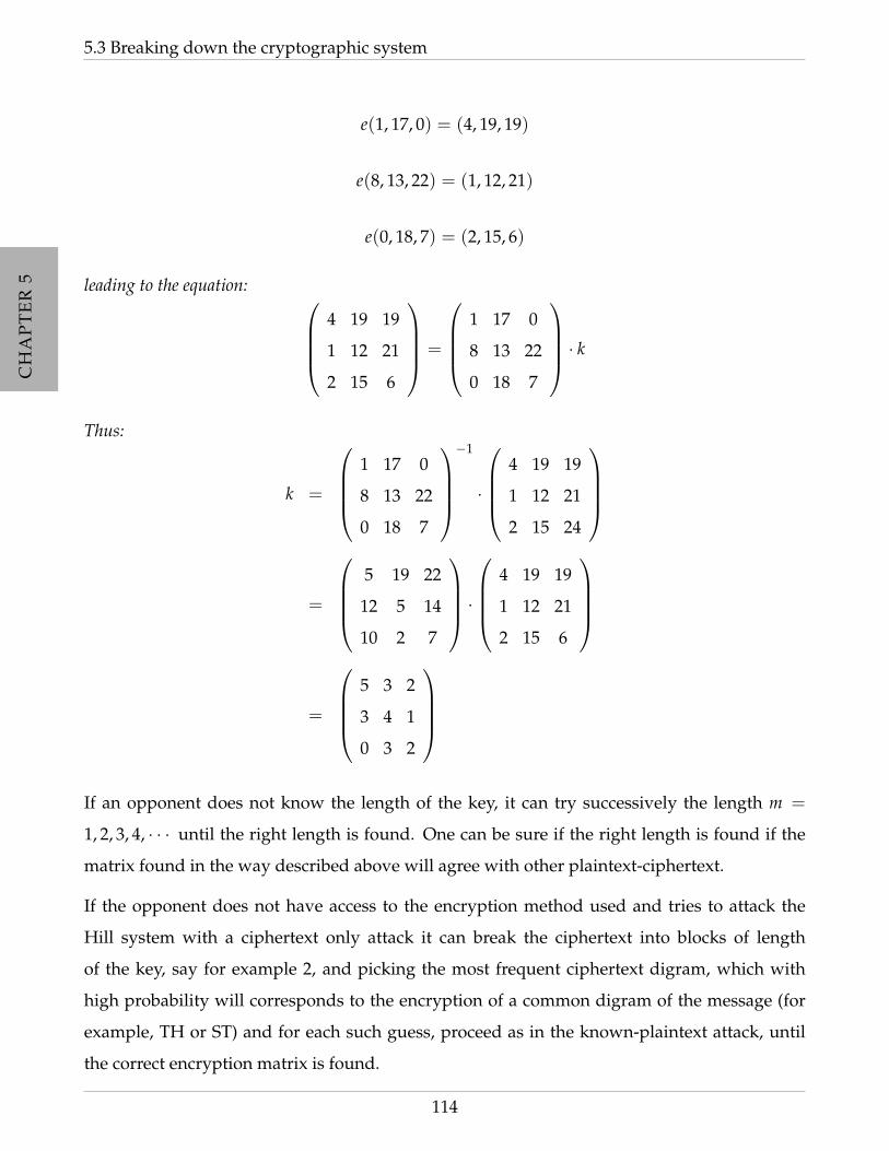
CH

AP

TE

R5

CH

AP

TE

R5

CH

AP

TE

R5

CH

AP

TE

R5


e(1, 17, 0) = (4, 19, 19)

e(8, 13, 22) = (1, 12, 21)

e(0, 18, 7) = (2, 15, 6)

leading to the equation: 4 19 19

1 12 21

2 15 6

=

1 17 0

8 13 22

0 18 7

· k

Thus:

k =

1 17 0

8 13 22

0 18 7

−1

·

4 19 19

1 12 21

2 15 24

=

5 19 22

12 5 14

10 2 7

·

4 19 19

1 12 21

2 15 6

=

5 3 2

3 4 1

0 3 2

If an opponent does not know the length of the key, it can try successively the length m =

1, 2, 3, 4, · · · until the right length is found. One can be sure if the right length is found if the

matrix found in the way described above will agree with other plaintext-ciphertext.

If the opponent does not have access to the encryption method used and tries to attack the

Hill system with a ciphertext only attack it can break the ciphertext into blocks of length

of the key, say for example 2, and picking the most frequent ciphertext digram, which with

high probability will corresponds to the encryption of a common digram of the message (for

example, TH or ST) and for each such guess, proceed as in the known-plaintext attack, until

the correct encryption matrix is found.

114

CH

AP

TE

R5

CH

AP

TE

R5

CH

AP

TE

R5

CH

AP

TE

R5


• • •

5.3.4 Breaking the LFCS

Recall that the ciphertext is obtained from the plaintext and the keystream by summing them

up modulo 2, i.e., yi = (xi + zi) (mod 2) and the keystream is produced from an initial key,

i.e., (z1, · · · , zm) = (k1, · · · , km), using a linear combination zm+i =m−1

∑j=0

cjzi+j (mod 2). This

can again be used to show that this cipher can be break with a known-plaintext attack.

Assume that an opponent has a plaintext x = x1 · · · xn and the corresponding ciphertext Y =

y1 · · · yn. Notice that, since yi = xi + zi (mod 2) then zi = yi + xi, so it is easy, in O knows

the length of the initial key of the keystream it is easy to recover it. All that is left to do is to

determine the keystream bits c0, · · · , cm1 in order to be able to reconstruct the entire keystream.

In other words, all that O has to determine the values of m unknowns. In fact, for any i > 1, by

the knowledge of the plaintext and the ciphertext one gets a linear equation in the m unknowns.

In the case of n > 2m the system

zm+i =m−1

∑j=0

cjzi+j (mod 2)

can be determined which can be rewritten in matrix form as follows:

(zm+1, · · · , z2m) = (c0, · · · , cm1)

z1 z2 · · · zm

z2 z3 · · · zm+1...

......

...

zm zm+1 · · · z2m

and if the matrix is invertible modulo 2 one can determine the coefficients c0, · · · , cm−1. No-

tice that the matrix has an inverse if m is the degree of the recurrence used to generate the

keystream.

115

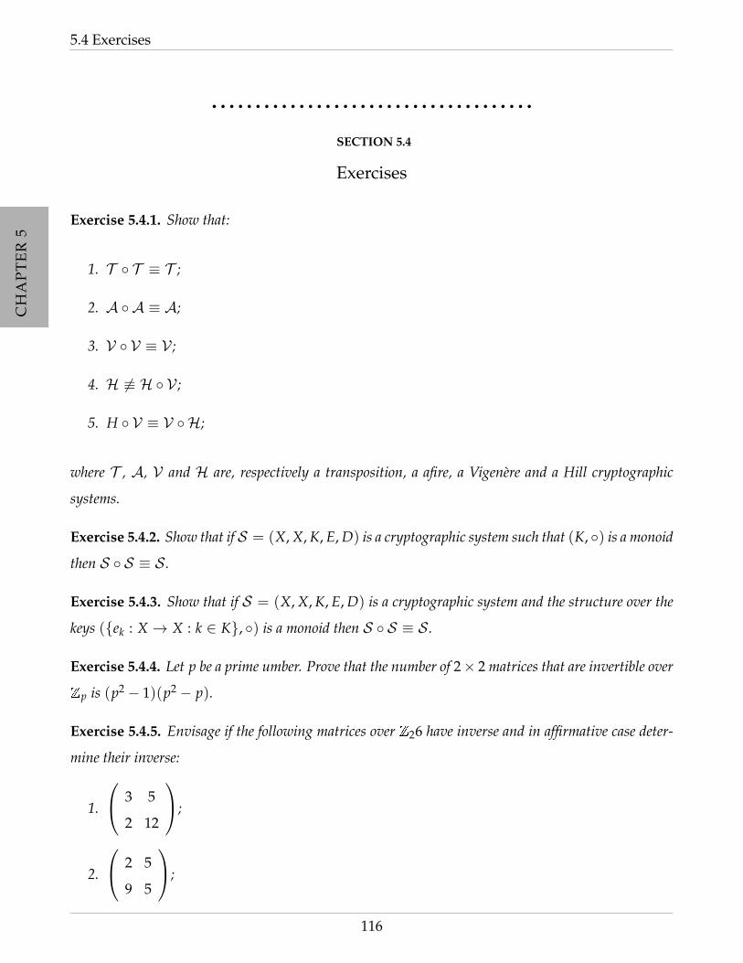
CH

AP

TE

R5

CH

AP

TE

R5

CH

AP

TE

R5

CH

AP

TE

R5

5.4 Exercises

• • • • • • • • • • • • • • • • • • • • • • • • • • • • • • • • • • • • •

SECTION 5.4

Exercises

Exercise 5.4.1. Show that:

1. T T ≡ T ;

2. A A ≡ A;

3. V V ≡ V ;

4. H 6≡ H V ;

5. H V ≡ V H;

where T , A, V and H are, respectively a transposition, a afire, a Vigenere and a Hill cryptographic

systems.

Exercise 5.4.2. Show that if S = (X, X, K, E, D) is a cryptographic system such that (K, ) is a monoid

then S S ≡ S .

Exercise 5.4.3. Show that if S = (X, X, K, E, D) is a cryptographic system and the structure over the

keys (ek : X → X : k ∈ K, ) is a monoid then S S ≡ S .

Exercise 5.4.4. Let p be a prime umber. Prove that the number of 2× 2 matrices that are invertible over

Zp is (p2 − 1)(p2 − p).

Exercise 5.4.5. Envisage if the following matrices over Z26 have inverse and in affirmative case deter-

mine their inverse:

1.

3 5

2 12

;

2.

2 5

9 5

;

116

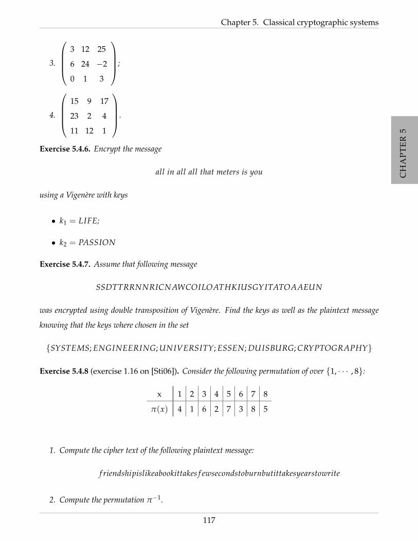
CH

AP

TE

R5

CH

AP

TE

R5

CH

AP

TE

R5

CH

AP

TE

R5


3.

3 12 25

6 24 −2

0 1 3

;

4.

15 9 17

23 2 4

11 12 1

.

Exercise 5.4.6. Encrypt the message

all in all all that meters is you

using a Vigenere with keys

• k1 = LIFE;

• k2 = PASSION

Exercise 5.4.7. Assume that following message

SSDTTRRNNRICNAWCOILOATHKIUSGYITATOAAEUN

was encrypted using double transposition of Vigenere. Find the keys as well as the plaintext message

knowing that the keys where chosen in the set

SYSTEMS; ENGINEERING; UNIVERSITY; ESSEN; DUISBURG; CRYPTOGRAPHY

Exercise 5.4.8 (exercise 1.16 on [Sti06]). Consider the following permutation of over 1, · · · , 8:

x 1 2 3 4 5 6 7 8

π(x) 4 1 6 2 7 3 8 5

1. Compute the cipher text of the following plaintext message:

f riendshipislikeabookittakes f ewsecondstoburnbutittakesyearstowrite

2. Compute the permutation π−1.

117

CH

AP

TE

R5

CH

AP

TE

R5

CH

AP

TE

R5

CH

AP

TE

R5

5.4 Exercises

3. Decrypt the following ciphertext:

TGEEMNELNNTDROEOAAHDOETCSHAEIRLM

Exercise 5.4.9. Show that the Shift cipher system presented in Exercise 5.1.5, the Substitution cipher

system presented in Cryptographic System 5.1.3 and the Vigenere cipher system presented in Crypto-

graphic System 5.1.9 are trivial to attack with a chosen plain text attack. Envisaged on least number of

characters needed to attack these cipher systems.

Exercise 5.4.10. Decode the following text knowing that was ciphered with a shift cipher system.

GUIOM UERJM MOWJQ OUEDF COQXD PRKBX QOXKV MCDLF COMJI IOQDA POKQD

EGUIO MOERO RMJER UBOER ORTVF CUEDF COQDP BILVW XDPRI ORUPA DQFCO

KOMFK UMNOF KUPPL PUBOQ VEFCO TDQPR UERCV MOPOY OEFOU IIUFO MOERO

RTVFC GUIOM GDVEV EXIVW CUOPG DQRUE VEDEO DAKUM NOFKU PPMID MFOSW

PJMVY OWPJK MFCOJ EVFOR MFUFO MDJFP UMFOR MLUVE KBMOY OELDV EFMAD

QVFMM OWDER MFQUV XCFXD PRIOR UPTVF CFCVQ FBLDV EFMAQ DINOY VERJQ

UEFUE RPUFO COQDV WMAQD IPOKQ DEGUI OMVEU EJEOS LOWFO RPBWP DMOXU

IO

Infer the title, and punctuation of the text.

Exercise 5.4.11. Decode the following text knowing that was ciphered with a substitution cipher system.

VGXYJ ZSAZY LYQVY FFSQJ YJSRU UWJJR UPZYV QZRAS ROYQJ ZSJZR ALWXX

RBSQW UQZSQ SUJVS JWSVY UNSFD WFFSP SRUDY VIARL PSYJX WNAJS SUGSY

AQWFL OZSAS RASQR LSLJZ ASSGS YAQYU LYCCF RSLVG QSFXD FWQSJ WVGQJ

NLRSQ INJJZ SDZYA PSWXV YRUJY RURUP VSYFJ ZWNPZ RZYLY BSAGQ DYUJG

YFFWO YUDSI SRUPJ WWPAS YJXWA YUYAA WOXWA JNUSR OYQIW NULYC CASUJ

RDSJW VATYV SQIYJ SQYUS VRUSU JQNAP SWURU FWULW UORJZ OZWVR DWUJR

UNSLX WNAGS YAQYU LVGXY JZSAU WOYUL JZSUQ SULRU PVSQV YFFQN VQWXV

WUSGR FYRLJ ZSVWN JRUFS YAURU PUYBR PYJRW UYULW JZSAC YAJQW XJZSV

YJZSV YJRDQ NQSXN FJWJZ WQSOZ WRUJS ULJWJ AYBSF YQRYF OYGQI SFRSB

SLRJO WNFLI SQWVS JRVSW AWJZS AVGXW AJNUS JWLW

118

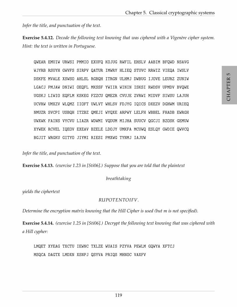
CH

AP

TE

R5

CH

AP

TE

R5

CH

AP

TE

R5

CH

AP

TE

R5



Exercise 5.4.12. Decode the following text knowing that was ciphered with a Vigenere cipher system.

Hint: the text is written in Portuguese.

QWEAR EMUIW URWSI PMMIO EXUFQ KOJUG RWFIL EHSLV AABIM BFQWD NSAVG

WJYRB RSUYH GWVFS SIRPV QATUR IMWRY HLIEQ STUVC RRWIZ VIEQA IWSLV

DSKFE MVALE XSWSO AHLSL RGBQH ITRGN ULHMJ DWBUG IJOVE LEURZ ZUNIW

LGACJ PMJAW DNIWI OEQFL MKSSF YWIIR WININ ISKSI RWDSV UPMDV BVQWE

UGSKJ LIWIO EQFLM KSKEG FZZCU QMEZR CVUJE ZVRWI MIDVF SIWSU LAJUH

UCVRW UMXZV WLQMZ IIOFT UWLVT WHLSV FDJYG IQICS DXEZV DGHWM URIEQ

NMUZR SVCPI USBQH ITZBZ QMEJI WYQXE ARPWY LELFH WBBEL FHADB EWRGH

UWXWK FAINS VYCVU LIAZR WDWMI VQDUM MIJHA SUUCV QGCJI BZOSK GEMUW

XYWEK RCVEL IQEOV EXEAV BZELE LDOJY UMKFA MCUWQ ESLQY GWDIE QWVCQ

BGJIT WRGKU GITYO JIYMI RIESI PMXWG TYNMJ IAJUW


Exercise 5.4.13. (exercise 1.23 in [Sti06].) Suppose that you are told that the plaintext

breathtaking

yields the ciphertext

RUPOTENTOIFV.

Determine the encryption matrix knowing that the Hill Cipher is used (but m is not specified).

Exercise 5.4.14. (exercise 1.25 in [Sti06].) Decrypt the following text knowing that was ciphered with

a Hill cypher:

LMQET XYEAG TXCTU IEWNC TXLZE WUAIS PZYVA PEWLM GQWYA XFTCJ

MSQCA DAGTX LMDXN XSNPJ QSYVA PRIQS MHNOC VAXFV

119

CH

AP

TE

R5

CH

AP

TE

R5

CH

AP

TE

R5

CH

AP

TE

R5

5.4 Exercises

120

CH

AP

TE

R6

CH

AP

TE

R6

CH

AP

TE

R6

CH

AP

TE

R6

CH

AP

TE

R6

CHAPTER 6

Perfect secrecy

In this chapter it is studied the influence of Shannon’s seminal paper on the notion of security of

a cryptographic systems. But what security means, i.e., what does it mean for a cryptographic

system to be secure?

In the previous chapter, some historical encryption schemes (ciphers) were presented and

showed how one can, with little computational effort, break them down. In this chapter,

it is studied conditions of the encryptions that are on the other extreme, i.e., it is studied

encryption schemes and conditions required by those systems that make them provably secure

even against an adversary who has unbounded computational power. Such schemes are called

perfectly secret.

Security is a term that is not easy to define clearly since it depends on the context where it

is considered and it is intrinsic to the kind of information one wants/needs to preserve. So,

security is a characteristic of the information and the communication process and, of course,

is definable depending on the goals the parties. For example if the goal in a communication

is to preserve ”privacy” of the message, then security is achieved if the information is kept

secret from everyone but the authorized people to see it. Some other examples of most used

”security” requirements are the following:

Data integrity: Make sure that the information of the message has not been altered by

unauthorized or unknown means.

121

CH

AP

TE

R6

CH

AP

TE

R6

CH

AP

TE

R6

CH

AP

TE

R6

CH

AP

TE

R6

Identification: Corroboration of the identity of an user.

Message authentication: Corroboration of the source of information.

Signature: The original owner of the message should be bind information to an entity.

Access control: The information of the message or segments of it should be confidential to

a restrictive access to resources to privileged entities.

Timestamping: The record of the time of creation or existence of information should be

kept invulnerable.

There are several approaches to measure informally the ”security” of a system:

Unconditional Security: This method is the ultimate goal of cryptography and thus ex-

cellent in theory. It means that there are no assumptions about the computing power

and resources available to an adversary and the system still be unbreakable leaking no

information whatsoever.

Provable Security: It is said that a system has provable security if its security requirements

can be stated formally in an adversarial model. Usually the proof of security of such

systems is the creation of a reduction from the assumptions about the adversary’s access

to the system to meet the security requirements stated for the system.

It is crucial to observe that this approach only ensures security relative to some other

problem, not an absolute proof of security. As an analogy think about a theorem: it is

only true if the assumptions are confirmed to hold, otherwise it might not be true.

Computational Security: In many cases, provable security cannot be realistically achieved,

and in such cases one must relax the security to computational security. Roughly speak-

ing this means that these systems are secure assuming that any adversaries are computa-

tionally limited. Formally this measure is related with the computational effort required

to break down the system i.e., the resources (time or space) that the best algorithm crack-

ing the system requires.

The security of a cryptographic system is related with the kind of attack that the opponent is

considering, as mentioned in the previous chapter. In the sequel it will be proved that certain

122

CH

AP

TE

R6

CH

AP

TE

R6

CH

AP

TE

R6

CH

AP

TE

R6

CH

AP

TE

R6

Chapter 6. Perfect secrecy

cryptographic systems are unconditionally secure against a ciphertext-only attack. In particu-

lar, a Shift Cipher or a Substitution Cipher or even the one time pad are both unconditionally

secure if a single element of plaintext is encrypted with a random key and the Vigenere Cipher

with keyword length m is unconditionally secure if the key is used to encrypt only one block

of the plaintext.

For that purpose, some mathematical definitions will be given and the unconditional security

with be rigorously proved, which gives some conditions os unconditional security without

relying on any unproven assumptions. Although the obvious advantages of this approach this

approach has inherent limitations.

• • • • • • • • • • • • • • • • • • • • • • • • • • • • • • • • • • • • •

SECTION 6.1

Definition of perfect security and results

To explain the concept of perfect secrecy and study in which conditions one says that a partic-

ular system has perfect secrecy several assumptions are made:

• The existence of a fixed cryptographic system (P, C, K, e, d) with the particularity that a

key k ∈ K is used for only one encryption.

• A fixed probability distribution over the plaintext space, P and thus the induced a so

called, a priori probability distribution of the plaintext elements, which is a random

variable, denoted by x.

• The key k is chosen using some fixed probability distribution which is often the uniform

one, and thus that one also has a random variable over the keys, denoted by k.

• The keys and the plain texts are independent random variables.

Since any ciphertext y is obtained from a plaintext and a key, i.e., y = dk(x) then the probability

distribution over K and the probability distribution X induce a probability distribution on C

and thus one can see the ciphertext elements as a random variable, which for convenience it is

denoted by y. Notice that, denoting by C(k) the set of possible ciphertexts that can be obtained

123

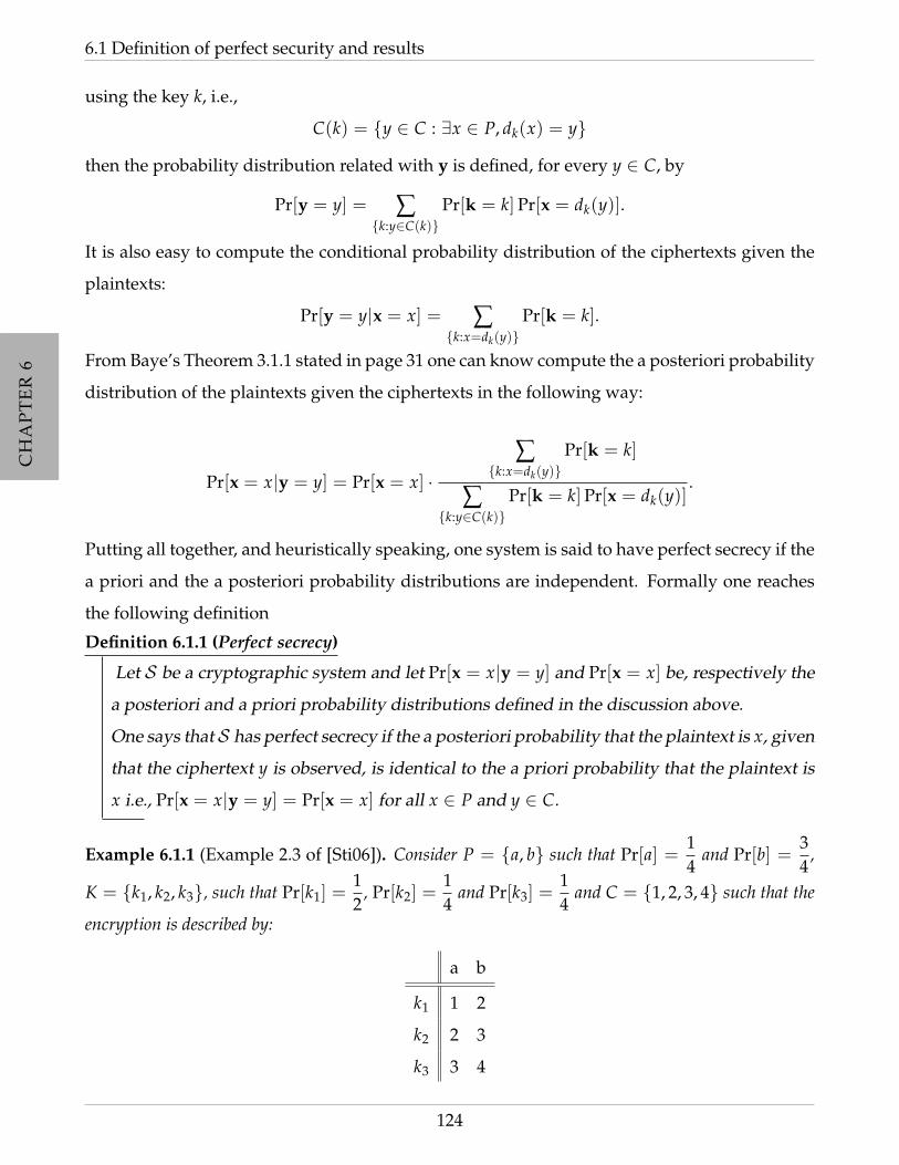
CH

AP

TE

R6

CH

AP

TE

R6

CH

AP

TE

R6

CH

AP

TE

R6

CH

AP

TE

R6

6.1 Definition of perfect security and results

using the key k, i.e.,

C(k) = y ∈ C : ∃x ∈ P, dk(x) = y

then the probability distribution related with y is defined, for every y ∈ C, by

Pr[y = y] = ∑k:y∈C(k)

Pr[k = k]Pr[x = dk(y)].

It is also easy to compute the conditional probability distribution of the ciphertexts given the

plaintexts:

Pr[y = y|x = x] = ∑k:x=dk(y)

Pr[k = k].

From Baye’s Theorem 3.1.1 stated in page 31 one can know compute the a posteriori probability

distribution of the plaintexts given the ciphertexts in the following way:

Pr[x = x|y = y] = Pr[x = x] ·∑

k:x=dk(y)Pr[k = k]

∑k:y∈C(k)

Pr[k = k]Pr[x = dk(y)].

Putting all together, and heuristically speaking, one system is said to have perfect secrecy if the

a priori and the a posteriori probability distributions are independent. Formally one reaches

the following definition

Definition 6.1.1 (Perfect secrecy)

Let S be a cryptographic system and let Pr[x = x|y = y] and Pr[x = x] be, respectively the

a posteriori and a priori probability distributions defined in the discussion above.

One says that S has perfect secrecy if the a posteriori probability that the plaintext is x, given

that the ciphertext y is observed, is identical to the a priori probability that the plaintext is

x i.e., Pr[x = x|y = y] = Pr[x = x] for all x ∈ P and y ∈ C.

Example 6.1.1 (Example 2.3 of [Sti06]). Consider P = a, b such that Pr[a] =14

and Pr[b] =34

,

K = k1, k2, k3, such that Pr[k1] =12

, Pr[k2] =14

and Pr[k3] =14

and C = 1, 2, 3, 4 such that the

encryption is described by:

a b

k1 1 2

k2 2 3

k3 3 4

124

CH

AP

TE

R6

CH

AP

TE

R6

CH

AP

TE

R6

CH

AP

TE

R6

CH

AP

TE

R6


Thus, for example, since 2 ∈ C(k1) ∪ C(k2) it follows that

Pr[y = 2] = Pr[k = k1]Pr[x = dk1(2)] + Pr[k = k2]Pr[x = dk2(2)]

= Pr[k = k1]Pr[x = b] + Pr[k = k2]Pr[x = a]

=12· 3

4+

14· 1

4

=7

16

The complete probability distribution of the random variable is:

Pr[y = 1] =18

Pr[y = 2] =7

16Pr[y = 3] =

14

Pr[y = 4] =1

16

For example the a posteriori probability of x = a given y = 3 can be computed in the following manner:

k : a = dk(y) = k2

and

k : y ∈ C(k) = k1, k2

thus:

Pr[x = x|y = y] = Pr[x = x] ·∑

k:x=dk(y)Pr[k = k]

∑k:y∈C(k)

Pr[k = k]Pr[x = dk(y)]

= Pr[x = a] · Pr[k = k2]

Pr[k = k1]Pr[x = dk1(2)] + Pr[k = k2]Pr[x = dk2(2)]

= Pr[x = a] · Pr[k = k2]

Pr[k = k1]Pr[x = b] + Pr[k = k2]Pr[x = a]

=14·

14

12· 3

4+

14· 1

4

=17

125

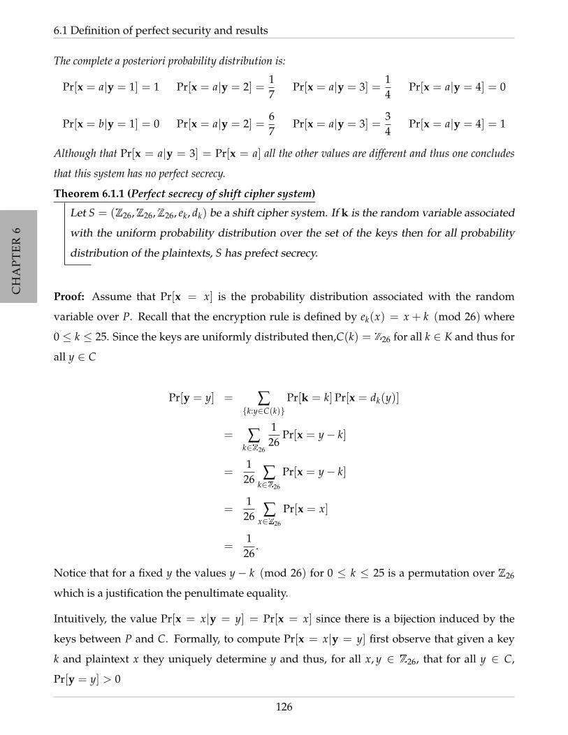
CH

AP

TE

R6

CH

AP

TE

R6

CH

AP

TE

R6

CH

AP

TE

R6

CH

AP

TE

R6


The complete a posteriori probability distribution is:

Pr[x = a|y = 1] = 1 Pr[x = a|y = 2] =17

Pr[x = a|y = 3] =14

Pr[x = a|y = 4] = 0

Pr[x = b|y = 1] = 0 Pr[x = a|y = 2] =67

Pr[x = a|y = 3] =34

Pr[x = a|y = 4] = 1

Although that Pr[x = a|y = 3] = Pr[x = a] all the other values are different and thus one concludes

that this system has no perfect secrecy.

Theorem 6.1.1 (Perfect secrecy of shift cipher system)

Let S = (Z26,Z26,Z26, ek, dk) be a shift cipher system. If k is the random variable associated

with the uniform probability distribution over the set of the keys then for all probability

distribution of the plaintexts, S has prefect secrecy.

Proof: Assume that Pr[x = x] is the probability distribution associated with the random

variable over P. Recall that the encryption rule is defined by ek(x) = x + k (mod 26) where

0 ≤ k ≤ 25. Since the keys are uniformly distributed then,C(k) = Z26 for all k ∈ K and thus for

all y ∈ C

Pr[y = y] = ∑k:y∈C(k)


= ∑k∈Z26

126

Pr[x = y− k]

=1

26 ∑k∈Z26

Pr[x = y− k]

=1

26 ∑x∈Z26

Pr[x = x]

=1

26.

Notice that for a fixed y the values y− k (mod 26) for 0 ≤ k ≤ 25 is a permutation over Z26

which is a justification the penultimate equality.

Intuitively, the value Pr[x = x|y = y] = Pr[x = x] since there is a bijection induced by the

keys between P and C. Formally, to compute Pr[x = x|y = y] first observe that given a key

k and plaintext x they uniquely determine y and thus, for all x, y ∈ Z26, that for all y ∈ C,

Pr[y = y] > 0

126

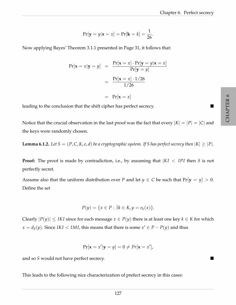
CH

AP

TE

R6

CH

AP

TE

R6

CH

AP

TE

R6

CH

AP

TE

R6

CH

AP

TE

R6


Pr[y = y|x = x] = Pr[k = k] =1

26.

Now applying Bayes’ Theorem 3.1.1 presented in Page 31, it follows that:

Pr[x = x|y = y] =Pr[x = x] · Pr[y = y|x = x]

Pr[y = y]

=Pr[x = x] · 1/26

1/26

= Pr[x = x]

leading to the conclusion that the shift cipher has perfect secrecy.

Notice that the crucial observation in the last proof was the fact that every |K| = |P| = |C| and

the keys were randomly chosen.

Lemma 6.1.2. Let S = (P, C, K, e, d) be a cryptographic system. If S has perfect secrecy then |K| ≥ |P|.

Proof: The proof is made by contradiction, i.e., by assuming that |KI < IPI then S is not

perfectly secret.

Assume also that the uniform distribution over P and let y ∈ C be such that Pr[y = y] > 0.

Define the set

P(y) = x ∈ P : ∃k ∈ K, y = ek(x).

Clearly |P(y)| ≤ IKI since for each message x ∈ P(y) there is at least one key k ∈ K for which

x = dk(y). Since IKI < IMI, this means that there is some x′ ∈ P− P(y) and thus

Pr[x = x′|y = y] = 0 6= Pr[x = x′],

and so S would not have perfect secrecy.

This leads to the following nice characterization of prefect secrecy in this cases:

127

CH

AP

TE

R6

CH

AP

TE

R6

CH

AP

TE

R6

CH

AP

TE

R6

CH

AP

TE

R6


Theorem 6.1.2 (Shannon’s theorem)

Let S = (P, C, K, e, d) be a cryptographic system such that |K| = |P| = |C| and such that

for all y ∈ C, Pr[y = y] > 0. Then S has perfect secrecy if and only if every key is uniformly

chosen with equal probability 1/|K|, and for every x ∈ P and every y ∈ C, there is a unique

key k such that ek(x) = y.

Notice that assuming that that for all y ∈ C, Pr[y = y] > 0 is a reasonable assumption since if

for some y ∈ C, Pr[y = y] = 0 this would mean that y is never used as a ciphertext and thus

one could consider C′ = C− y without loss of generality.

Proof:

(⇐)

Since for all y ∈ C, Pr[y = y] > 0 and the distributions x and y are independent, then for all

x and y, Pr[y = y|x = x] = Pr[y = y] > 0 and hence there is at least one k ∈ K such that

ek(x) = y and thus |C| = |ek(x) : k ∈ K| ≤ |K|.

Notice that fixing an x, the function

keyx : K → Y

k → ek(x)

is then surjective and since |K| = |C| it follows that |ek(x) : k ∈ K| = |K| which implies

that it is also injective and thus, it cannot exist two distinct keys k1 and k2 such that ek1(x) =

ek2(x) = y. This leads to the conclusion that for any x ∈ P and y ∈ C, there is exactly one key k

such that ek(x) = y.

Assume that |K| = |P| = |C| = n and assume that the elements of P are ordered, i.e., P = xi :

1 ≤ i ≤ n. Given y one can enumerate the keys in the following way: eki(xi) = y.

By Bayes’ Theorem 3.1.1 presented in page 31, one has:

Pr[x = xi|y = y] =Pr[y = y|x = xi]Pr[x = xi]

Pr[y = y]

=Pr[k = ki]Pr[x = xi]

Pr[y = y].

128

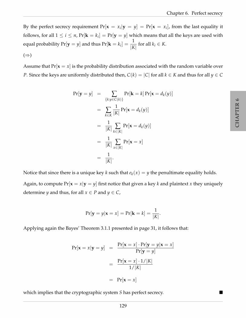
CH

AP

TE

R6

CH

AP

TE

R6

CH

AP

TE

R6

CH

AP

TE

R6

CH

AP

TE

R6


By the perfect secrecy requirement Pr[x = xi|y = y] = Pr[x = xi], from the last equality it

follows, for all 1 ≤ i ≤ n, Pr[k = ki] = Pr[y = y] which means that all the keys are used with

equal probability Pr[y = y] and thus Pr[k = ki] =1|K| for all ki ∈ K.

(⇒)

Assume that Pr[x = x] is the probability distribution associated with the random variable over

P. Since the keys are uniformly distributed then, C(k) = |C| for all k ∈ K and thus for all y ∈ C

Pr[y = y] = ∑k:y∈C(k)


= ∑k∈K

1|K| Pr[x = dk(y)]

=1|K| ∑

k∈|K|Pr[x = dk(y)]

=1|K| ∑

x∈|K|Pr[x = x]

=1|K| .

Notice that since there is a unique key k such that ek(x) = y the penultimate equality holds.

Again, to compute Pr[x = x|y = y] first notice that given a key k and plaintext x they uniquely

determine y and thus, for all x ∈ P and y ∈ C,

Pr[y = y|x = x] = Pr[k = k] =1|K| .

Applying again the Bayes’ Theorem 3.1.1 presented in page 31, it follows that:

Pr[x = x|y = y] =Pr[x = x] · Pr[y = y|x = x]

Pr[y = y]

=Pr[x = x] · 1/|K|

1/|K|

= Pr[x = x]

which implies that the cryptographic system S has perfect secrecy.

129

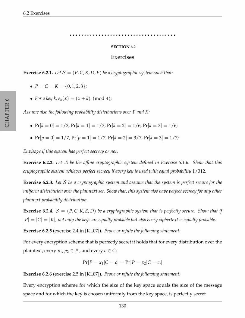
CH

AP

TE

R6

CH

AP

TE

R6

CH

AP

TE

R6

CH

AP

TE

R6

CH

AP

TE

R6

6.2 Exercises

• • • • • • • • • • • • • • • • • • • • • • • • • • • • • • • • • • • • •

SECTION 6.2

Exercises

Exercise 6.2.1. Let S = (P, C, K, D, E) be a cryptographic system such that:

• P = C = K = 0, 1, 2, 3;

• For a key k, ek(x) = (x + k) (mod 4);

Assume also the following probability distributions over P and K:

• Pr[k = 0] = 1/3, Pr[k = 1] = 1/3, Pr[k = 2] = 1/6, Pr[k = 3] = 1/6;

• Pr[p = 0] = 1/7, Pr[p = 1] = 1/7, Pr[k = 2] = 3/7, Pr[k = 3] = 1/7;

Envisage if this system has perfect secrecy or not.

Exercise 6.2.2. Let A be the affine cryptographic system defined in Exercise 5.1.6. Show that this

cryptographic system achieves perfect secrecy if every key is used with equal probability 1/312.

Exercise 6.2.3. Let S be a cryptographic system and assume that the system is perfect secure for the

uniform distribution over the plaintext set. Show that, this system also have perfect secrecy for any other

plaintext probability distribution.

Exercise 6.2.4. S = (P, C, K, E, D) be a cryptographic system that is perfectly secure. Show that if

|P| = |C| = |K|, not only the keys are equally probable but also every ciphertext is equally probable.

Exercise 6.2.5 (exercise 2.4 in [KL07]). Prove or refute the following statement:

For every encryption scheme that is perfectly secret it holds that for every distribution over the

plaintext, every p1, p2 ∈ P , and every c ∈ C:

Pr[P = x1|C = c] = Pr[P = x2|C = c.]

Exercise 6.2.6 (exercise 2.5 in [KL07]). Prove or refute the following statement:

Every encryption scheme for which the size of the key space equals the size of the message

space and for which the key is chosen uniformly from the key space, is perfectly secret.

130

CH

AP

TE

R6

CH

AP

TE

R6

CH

AP

TE

R6

CH

AP

TE

R6

CH

AP

TE

R6


Exercise 6.2.7 (exercise 2.9 in [KL07]). Consider the following definition of perfect secrecy for the

encryption of two messages.

An encryption scheme over a plaintext space P is perfectly-secret for two messages if for all

distributions over P, all p, p′ ∈ P and all c, c′ ∈ C such that Pr[C = c ∧ C′ = c′] > 0

Pr[P = p ∧ P = p′|C = c ∧ C′ = c′] = Pr[P = p ∧ P = p′]

where p and p′ are sampled independently from the same distribution over P.

Prove that no encryption scheme satisfies this definition. (Hint: Take p 6= p′ but c = c′.)

Exercise 6.2.8. There are other ways of defining perfect secrecy. In [KL07] the authors proposed the

following alternative notion of perfect secrecy:

Consider the an experiment called PriveavK which considers the a private-key encryption and

an eavesdropping opponent that only has access to a ciphertext c and then tries to determine

something about the plaintext that originates c. The experiment is defined for any encryption

scheme over plaintext P and for any adversary A and let PriveavK,Π denote an execution of the

experiment for a given Π and A defined as follows:

1. The adversary A outputs a pair of messages p0, p1 ∈ P.

2. A uniformly random key k is generated, and a uniformly random bit b ∈ 0, 1 is chosen.

Then, the ciphertext c = ek(pb) is computed and given to A.?

3. A outputs a bit b′.

The output of the experiment are: PriveavK,Π = 1 if b′ = b, and 0 otherwise. Comment: One

should think of A as trying to guess the value of b that is chosen in the experiment, and A succeeds

when its guess b′ is correctly. Observe that it is always possible for A to succeed in the experiment with

probability one half by just guessing b′ randomly. One says that the encryption is perfect secure if this

is the best probability that the adversary has to infer the bit used.

Prove that this definition is equivalent to the Definition 6.1.1 presented on Page 124.

131

CH

AP

TE

R6

CH

AP

TE

R6

CH

AP

TE

R6

CH

AP

TE

R6

CH

AP

TE

R6

6.2 Exercises

132

CH

AP

TE

R7

CH

AP

TE

R7

CH

AP

TE

R7

CH

AP

TE

R7

CH

AP

TE

R7

CH

AP

TE

R7

CHAPTER 7

Block ciphers: DES and AES

In this chapter it will be used the notion of product cipher system to explain and construct the

system and the system AES, respectively, Data Encryption Standard and Advanced Encryption

Standard. From a block cipher one expects that it should behave like a random permutation to

provide diffusion and confusion and in this way prevent the vast majority of known practical

attacks. Notice that a truly random permutation would be desirable but its representation for

an input of size n would require log(2n!) ≈ 2n which is impractical for n > 20 and completely

unfeasible for n > 50. Thus, one need to construct a concise function that behaves like a

random one.

The idea of block ciphers is to consider a block of plaintext and transform it at once into a

block of a ciphertext. To begin it is explained an iterated cipher that typically consists on an

application of a function g, properly named round function, for a specific number of rounds,

say Nr, and a key schedule (K1, · · · , kNr) that usually is formed from a initial key K and a

public algorithm to construct each Ki, the subkey for each round from K. Notice that from

the name of the schemes, iterated ciphers, the function g, each takes a code and a key and

produces another code, must have the property that the set of the original code must contain

the range set of the original code, since it works by taking a a subkey Kr and a current code

wr−1 and produces the code wr = g(wr−1, Kr). The initial code, w0 is the plaintext and wNr is

the ciphertext. Another important feature of g, in order to all decryption, it must be injective

133

CH

AP

TE

R7

CH

AP

TE

R7

CH

AP

TE

R7

CH

AP

TE

R7

CH

AP

TE

R7

CH

AP

TE

R7

7.1 Substitution-Permutation Networks

for each key, i.e., when a key is fixed, one can compute g−1k (g(w, k)) = w for all w.

In the next section it is presented the Substitution-Permutation Networks that are examples of

iterated cipher systems that have most of the basic ideas to construct the DES and AES.

• • • • • • • • • • • • • • • • • • • • • • • • • • • • • • • • • • • • •

SECTION 7.1

Substitution-Permutation Networks

In the last Chapter the notion of secrecy was studied as an important contribute of Shannon

to the analyses of security of cipher system. In addition to this contribution, Shannon also

introduced the confusion-diffusion paradigm which aims to construct concise random look-

ing permutations with a large block length from many smaller random (or random looking)

permutations with small block length. In this case, diffusion means a method of dissipate the

statistical structure of the plaintext hiding the redundancy in the ciphertext. Also, confusion is

used to make the relation between the simple statistics of ciphertext and the simple description

of the key a very complex and involved one. One way of realizing Shannon’s principles is the

so called substitution permutation network (SPN) cryptographic system.

An SPN cryptographic system consists of Nr rounds, each of them made up of a substitution

stage and a permutation stage. The idea of an SPN is that the repetition of confusion and

diffusion in each round ensures that any small change in the input will be mixed throughout

the entire process and will affect all or almost all the bits of the output. Thus, the effect of small

changes in the input have a significant effect on the output similarly to what one would expect

to happen with the use of a random permutation.

Letting, l and m be two integers. The plaintext and ciphertext are binary strings of length lm.

In the substitution stage is a permutation πS : 0, 1l → 0, 1l and is used to replace l bits

with a different set of l bits. In the permutation stage, like the name suggests is a permutation

πP : 0, 1lm → 0, 1lm used to permute lm bits.

The idea is to consider a lm bit string corresponding to a plain text x and divide it into m blocks

of l-bit strings denoted by x〈1〉, · · · , x〈lm〉 where x〈i〉 = x(i−1)l, · · · , xil.

In each of Nr rounds (except for the last round, which is slightly different), first the subkey ki is

134

CH

AP

TE

R7

CH

AP

TE

R7

CH

AP

TE

R7

CH

AP

TE

R7

CH

AP

TE

R7

CH

AP

TE

R7

Chapter 7. Block ciphers: DES and AES

incorporated via and then perform m substitutions using πS, followed by a permutation using

πP. The complete description of the cryptographic system is presented in the following.

Cryptographic system 7.1.1 (Substitution-Permutation Network)

Let L, m and Nr be three non null integers. Consider also πS : 0, 1l → 0, 1l and

πP : 0, 1lm → 0, 1lm two permutation. The Substitution-Permutation Network crypto-

graphic system is the tuple (P, C, K, E, D) where P = C = 0, llm, and K ⊂ (0, 1lm)Nr+1

consists of all possible key schedules that could be derived from an initial key k using

a public key scheduling algorithm. For a key schedule (k1, · · · , kNr+1), the encryption

function is described as follows.

Algorithm 7.1.2 (SPN encryption function)

Input: The plaintext x, the permutations πS and πS and the key scheduling

(k1, · · · , kNr+1).

Output: The ciphertext y.

Step 1: w0 = x;

Step 2: for r = 1 to Nr− 1 do:

Step 2.1: ur = wr−1 ⊕ Kr;

Step 2.2: for i = 1 to m do:

Step 2.2.1: vr〈i〉 = πS(ur

〈i〉)

Step 2.3: wr = vrπP(1)

· · · vrπP(lm)

Step 3: uNr = wNr−1 ⊕ KNr;

Step 4: for i = 1 to m do:

Step 4.1: vNr〈i〉 = πS(uNr

〈i〉 )

Step 5: y = vNr ⊕ kNr+1.

Notice that the very first and last operations performed in this SPN are x-ors with subkeys.

This is called whitening, and is regarded as a useful way to prevent an attacker from even

beginning to carry out an encryption or decryption operation if the key is not known.

135

CH

AP

TE

R7

CH

AP

TE

R7

CH

AP

TE

R7

CH

AP

TE

R7

CH

AP

TE

R7

CH

AP

TE

R7


Example 7.1.3 (Example 3.1 of [Sti06]). This SPN cryptographic system is represented in schemati-

cally represented in next figure:

Figure 7.1: Scheme of the SPN of the example

136

CH

AP

TE

R7

CH

AP

TE

R7

CH

AP

TE

R7

CH

AP

TE

R7

CH

AP

TE

R7

CH

AP

TE

R7


The parameters for the SPN are:

m= 4

l= 4

Nr= 4

Substitution permutation: It is the following permutation over 0, 14

x

0

0

0

0

0

0

0

1

0

0

1

0

0

0

1

1

0

1

0

0

0

1

0

1

0

1

1

0

0

1

1

1

1

0

0

0

1

0

0

1

1

0

1

0

1

0

1

1

1

1

0

0

1

1

0

1

1

1

1

0

1

1

1

1

πS(x)

1

1

1

0

0

1

0

0

1

1

0

1

0

0

0

1

0

0

1

0

1

1

1

1

1

0

1

1

1

0

0

0

0

0

1

1

1

0

1

0

0

1

1

0

1

1

0

0

0

1

0

1

1

0

0

1

0

0

0

0

0

1

1

1

The other permutation: It is the following permutation over 1, · · · , 16

x 1 2 3 4 5 6 7 8 9 10 11 12 13 14 15 16

πP(x) 1 5 9 13 2 6 10 14 3 7 11 15 4 8 12 16

Key scheduling: Given a 32-bit key k = 0011 1010 1001 0100 1101 0110 0011 1111 all the

5 subkeys are constructed by considering 16 consecutive bits of k, beginning with the bit k4r−3,

where 1 ≤ r ≤ 4 i.e.,k1 = 0011 1010 1001 01001

k2 = 1010 1001 0100 1101

k3 = 1001 0100 1101 01101

k4 = 0100 1101 0110 0011

k5 = 1101 0110 0011 1111

plaintext: x = 0010 0110 1011 0111.

137

CH

AP

TE

R7

CH

AP

TE

R7

CH

AP

TE

R7

CH

AP

TE

R7

CH

AP

TE

R7

CH

AP

TE

R7


Now it is described roughly the trace of the Algorithm 7.1.2:

Step 1: w0 = x = 0010 0110 1011 0111;

Step 2-cicle 1:

xor with the subkey u1 = w0 ⊕ k1

= 0010 0110 1011 0111⊕ 0011 1010 1001 0100

= 0001 1100 0010 0011

applying πS v1 = 0100 0101 1101 0001

applying πP w1 = 0010 1110 0000 0111

Step 2-cicle 2:


= 0001 1100 0010 0011⊕ 1010 1001 0100 1101

= 1000 0111 0100 1010

applying πS v2 = 0011 1000 0010 0110

applying πP w2 = 0100 0001 1011 1000

Step 2-cicle 1:


= 0100 0001 1011 1000⊕ 1001 0100 1101 0110

= 1101 0101 0110 1110

applying πS v3 = 1001 1111 1011 0000

applying πP w3 = 1110 0100 0110 1110

138

CH

AP

TE

R7

CH

AP

TE

R7

CH

AP

TE

R7

CH

AP

TE

R7

CH

AP

TE

R7

CH

AP

TE

R7


Step 3:


= 1110 0100 0110 1110⊕ 0100 1101 0110 0011

= 1010 1001 0000 1101

Step 4:

applying πS v4 = 0110 1010 1110 1001

Step 5:

xor with the subkey y = v4 ⊕ k5

= 0110 1010 1110 1001⊕ 1101 0110 0011 1111

= 1011 1100 1101 0110

• • • • • • • • • • • • • • • • • • • • • • • • • • • • • • • • • • • • •

SECTION 7.2

DES – Data Encryption Standards

The Data Encryption Standard or simply DES is the result of efforts of IBM to the call on May 15,

1973, of the National Bureau of Standards, nowadays the National Institute of Standards and

Technology (NIST) request in the Federal Register for an encryption algorithm with following

properties:

• have a high security level related to a small key used for encryption and decryption;

• be easily understood;

• independent of the algorithm’s confidentiality;

• be adaptable and economical;

• be efficient and exportable.

139

CH

AP

TE

R7

CH

AP

TE

R7

CH

AP

TE

R7

CH

AP

TE

R7

CH

AP

TE

R7

CH

AP

TE

R7

7.2 DES – Data Encryption Standards

The DES was standardized by the ANSI (American National Standard Institute) under the

name of ANSI X3.92, better known as DEA (Data Encryption Algorithm) and was published

in the Federal Register of March 17, 1975. In 1976, after consultation of the National Security

Agency (NSA) and public discussion was published as an official Federal Information Process-

ing Standard (FIPS) for the United States in January 15, 1977 for “unclassified” applications.

The publication of an NSA-approved encryption standard simultaneously resulted in its quick

international adoption and widespread academic scrutiny. Also some criticism was presented

since there were made statements that the NSA could break any code of DES using a backdoor.

This algorithm was initially expected to be used as a standard for 10-15 years, however, it

proved to be much more durable and is reviewed approximately every five years. Its last

renewal was in January 1999.

DES is now considered to be insecure mainly because the 56-bit key size being too small. In

January, 1999, distributed.net and the Electronic Frontier Foundation collaborated to publicly

break a DES key in 22 hours and 15 minutes. There are also some analytical results which

demonstrate theoretical weaknesses in the cipher, although they are infeasible to mount in

practice. Other than exhaustive key search, the two most important cryptanalytic attacks on

DES are differential cryptanalysis and linear cryptanalysis. (For SPNs, theseThe algorithm is

for now computationally secure in the form of Triple DES, although there are known theo-

retical attacks. In recent years, the cipher has been superseded by the Advanced Encryption

Standard (AES) and has been withdrawn as a standard by the National Institute of Standards

and Technology.

• • •

7.2.1 Description of DES

As it was already mentioned the complete description of the Data Encryption Standard was

publish in January 15, 1977 in the Federal Information Processing Standards (FIPS) Publication

46 [oST99] and it can be roughly described by its central block consisting of four operations:

1. key generation;

2. key mixing;

140

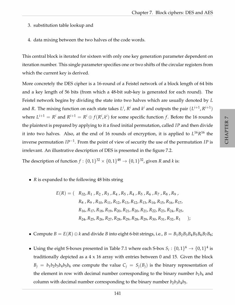
CH

AP

TE

R7

CH

AP

TE

R7

CH

AP

TE

R7

CH

AP

TE

R7

CH

AP

TE

R7

CH

AP

TE

R7


3. substitution table lookup and

4. data mixing between the two halves of the code words.

This central block is iterated for sixteen with only one key generation parameter dependent on

iteration number. This single parameter specifies one or two shifts of the circular registers from

which the current key is derived.

More concretely the DES cipher is a 16-round of a Feistel network of a block length of 64 bits

and a key length of 56 bits (from which a 48-bit sub-key is generated for each round). The

Feistel network begins by dividing the state into two halves which are usually denoted by L

and R. The mixing function on each state takes Li, Ri and ki and outputs the pair (Li+1, Ri+1)

where Li+1 = Ri and Ri+1 = Ri ⊕ f (Ri, ki) for some specific function f . Before the 16 rounds

the plaintext is prepared by applying to it a fixed initial permutation, called IP and then divide

it into two halves. Also, at the end of 16 rounds of encryption, it is applied to L16R16 the

inverse permutation IP−1. From the point of view of security the use of the permutation IP is

irrelevant. An illustrative description of DES is presented in the figure 7.2.

The description of function f : 0, 132 × 0, 148 → 0, 132, given R and k is:

• R is expanded to the following 48 bits string

E(R) = ( R32, R1 , R2 , R3 , R4 , R5 , R4 , R5 , R6 , R7 , R8 , R9 ,

R8 , R9 , R10, R11, R12, R13, R12, R13, R14, R15, R16, R17,

R16, R17, R18, R19, R20, R21, R20, R21, R22, R23, R24, R25,

R24, R25, R26, R27, R28, R29, R28, R29, R30, R31, R32, R1 );

• Compute B = E(R)⊕ k and divide B into eight 6-bit strings, i.e., B = B1B2B3B4B5B6B7B8;

• Using the eight S-boxes presented in Table 7.1 where each S-box Si : 0, 16 → 0, 14 is

traditionally depicted as a 4 x 16 array with entries between 0 and 15. Given the block

Bj = b1b2b3b4b5b6 one compute the value Cj = Sj(Bj) is the binary representation of

the element in row with decimal number corresponding to the binary number b1b6 and

column with decimal number corresponding to the binary number b2b3b4b5.

141

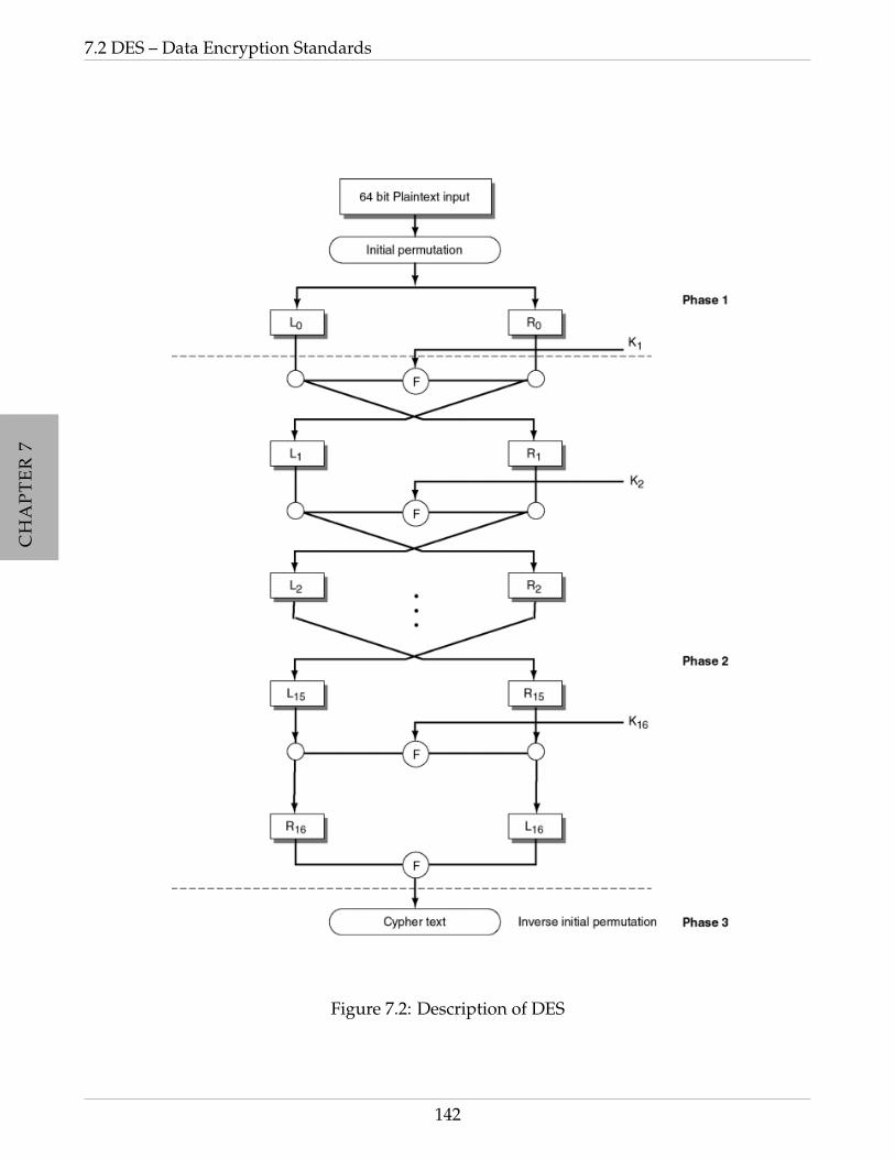
CH

AP

TE

R7

CH

AP

TE

R7

CH

AP

TE

R7

CH

AP

TE

R7

CH

AP

TE

R7

CH

AP

TE

R7


Figure 7.2: Description of DES

142

CH

AP

TE

R7

CH

AP

TE

R7

CH

AP

TE

R7

CH

AP

TE

R7

CH

AP

TE

R7

CH

AP

TE

R7


S1

b2b3b4b5 b1b2

0 1 2 3 4 5 6 7 8 9 10 11 12 13 14 15

14 4 13 1 2 15 11 8 3 10 6 12 5 9 0 7 00

0 15 7 4 14 2 13 1 10 6 12 11 9 5 3 8 01

4 1 14 8 13 6 2 11 15 12 9 7 3 10 5 0 10

15 12 8 2 4 9 1 7 5 11 3 14 10 0 6 13 11

S2

b2b3b4b5 b1b2

0 1 2 3 4 5 6 7 8 9 10 11 12 13 14 15

15 1 8 14 6 11 3 4 9 7 2 13 12 0 5 10 00

3 13 4 7 15 2 8 14 12 0 1 10 6 9 11 5 01

0 14 7 11 10 4 13 1 5 8 12 6 9 3 2 15 10

13 8 10 1 3 15 4 2 11 6 7 12 0 5 14 9 11

S3

b2b3b4b5 b1b2

0 1 2 3 4 5 6 7 8 9 10 11 12 13 14 15

10 0 9 14 6 3 15 5 1 13 12 7 11 4 2 8 00

13 7 0 9 3 4 6 10 2 8 5 14 12 11 15 1 01

13 6 4 9 8 15 3 0 11 1 2 12 5 10 14 7 10

1 10 13 0 6 9 8 7 4 15 14 3 11 5 2 12 11

S4

b2b3b4b5 b1b2

0 1 2 3 4 5 6 7 8 9 10 11 12 13 14 15

7 13 14 3 0 6 9 10 1 2 8 5 11 12 4 15 00

13 8 11 5 6 15 0 3 4 7 2 12 1 10 14 9 01

10 6 9 0 12 11 7 13 15 1 3 14 5 2 8 4 10

3 15 0 6 10 1 13 8 9 4 5 11 12 7 2 14 11

143

CH

AP

TE

R7

CH

AP

TE

R7

CH

AP

TE

R7

CH

AP

TE

R7

CH

AP

TE

R7

CH

AP

TE

R7


S5

b2b3b4b5 b1b2

0 1 2 3 4 5 6 7 8 9 10 11 12 13 14 15

2 12 4 1 7 10 11 6 8 5 3 15 13 0 14 9 00

14 11 2 12 4 7 13 1 5 0 15 10 3 9 8 6 01

4 2 1 11 10 13 7 8 15 9 12 5 6 3 0 14 10

11 8 12 7 1 14 2 13 6 15 0 9 10 4 5 3 11

S6

b2b3b4b5 b1b2

0 1 2 3 4 5 6 7 8 9 10 11 12 13 14 15

12 1 10 15 9 2 6 8 0 13 3 4 14 7 5 11 00

10 15 4 2 7 12 9 5 6 1 13 14 0 11 3 8 01

9 14 15 5 2 8 12 3 7 0 4 10 1 13 11 6 10

4 3 2 12 9 5 15 10 11 14 1 7 6 0 8 13 11

S7

b2b3b4b5 b1b2

0 1 2 3 4 5 6 7 8 9 10 11 12 13 14 15

4 11 2 14 15 0 8 13 3 12 9 7 5 10 6 1 00

13 0 11 7 4 9 1 10 14 3 5 12 2 15 8 6 01

1 4 11 13 12 3 7 14 10 15 6 8 0 5 9 2 10

6 11 13 8 1 4 10 7 9 5 0 15 14 2 3 12 11

S8

b2b3b4b5 b1b2

0 1 2 3 4 5 6 7 8 9 10 11 12 13 14 15

13 2 8 4 6 15 11 1 10 9 3 14 5 0 12 7 00

1 15 13 8 10 3 7 4 12 5 6 11 0 14 9 2 01

7 11 4 1 9 12 14 2 0 6 10 13 15 3 5 8 10

2 1 14 7 4 10 8 13 15 12 9 0 3 5 6 11 11

Table 7.1: The eight DES S – boxes

144

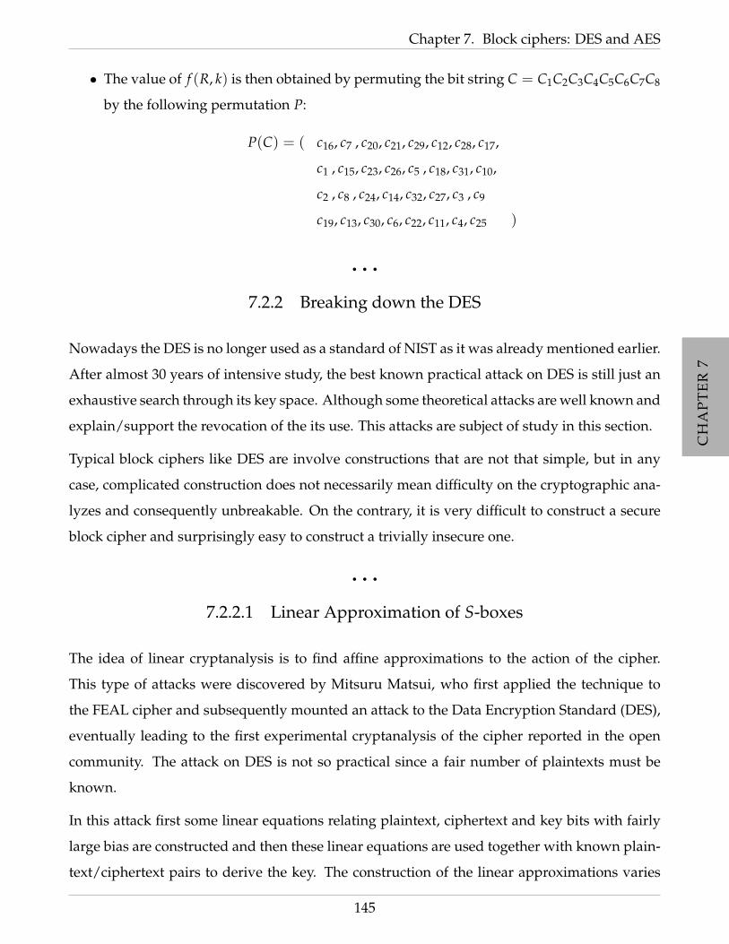
CH

AP

TE

R7

CH

AP

TE

R7

CH

AP

TE

R7

CH

AP

TE

R7

CH

AP

TE

R7

CH

AP

TE

R7


• The value of f (R, k) is then obtained by permuting the bit string C = C1C2C3C4C5C6C7C8

by the following permutation P:

P(C) = ( c16, c7 , c20, c21, c29, c12, c28, c17,

c1 , c15, c23, c26, c5 , c18, c31, c10,

c2 , c8 , c24, c14, c32, c27, c3 , c9

c19, c13, c30, c6, c22, c11, c4, c25 )

• • •

7.2.2 Breaking down the DES

Nowadays the DES is no longer used as a standard of NIST as it was already mentioned earlier.

After almost 30 years of intensive study, the best known practical attack on DES is still just an

exhaustive search through its key space. Although some theoretical attacks are well known and

explain/support the revocation of the its use. This attacks are subject of study in this section.

Typical block ciphers like DES are involve constructions that are not that simple, but in any

case, complicated construction does not necessarily mean difficulty on the cryptographic ana-

lyzes and consequently unbreakable. On the contrary, it is very difficult to construct a secure

block cipher and surprisingly easy to construct a trivially insecure one.

• • •

7.2.2.1 Linear Approximation of S-boxes

The idea of linear cryptanalysis is to find affine approximations to the action of the cipher.

This type of attacks were discovered by Mitsuru Matsui, who first applied the technique to

the FEAL cipher and subsequently mounted an attack to the Data Encryption Standard (DES),

eventually leading to the first experimental cryptanalysis of the cipher reported in the open

community. The attack on DES is not so practical since a fair number of plaintexts must be

known.

In this attack first some linear equations relating plaintext, ciphertext and key bits with fairly

large bias are constructed and then these linear equations are used together with known plain-

text/ciphertext pairs to derive the key. The construction of the linear approximations varies

145

CH

AP

TE

R7

CH

AP

TE

R7

CH

AP

TE

R7

CH

AP

TE

R7

CH

AP

TE

R7

CH

AP

TE

R7


x

0

0

0

0

0

0

0

1

0

0

1

0

0

0

1

1

0

1

0

0

0

1

0

1

0

1

1

0

0

1

1

1

1

0

0

0

1

0

0

1

1

0

1

0

1

0

1

1

1

1

0

0

1

1

0

1

1

1

1

0

1

1

1

1

πS(x)

1

1

1

0

0

1

0

0

1

1

0

1

0

0

0

1

0

0

1

0

1

1

1

1

1

0

1

1

1

0

0

0

0

0

1

1

1

0

1

0

0

1

1

0

1

1

0

0

0

1

0

1

1

0

0

1

0

0

0

0

0

1

1

1

1 1 1 1 0 1 1 1 1 0 1 1 1 1 1 1

X3 ⊕ X4 ⊕ Y1 ⊕ Y2

Table 7.2: Computation of the random variable X3 ⊕ X4 ⊕ Y1 ⊕ Y2

with the cipher used but in the case of the substitution-permutation network, the analysis is

concentrated primarily on the S-boxes, the only part of the system that is not linear (i.e. the

involved operation in an S-box cannot be encoded in a linear equation) and for a small S-boxes,

it is feasible to enumerate every possible linear equation which relate the input and output bits

of the boxes and thus determining their bias. For sake of presentation and understanding this

attack will be explained continuing the Example 7.1.3.

Example 7.2.1 (continuing over Example 7.1.3). The S-box used in the example is a permutation

πS : 0, 14 → 0, 14 and choosing X1, X2, X3 and X4 independently and uniformly at random one

can compute the the bias of the random variables X3 ⊕ X4 ⊕ Y1 ⊕ Y2. See the Table 7.2 for details.

εX3⊕X4⊕Y1⊕Y2 = Pr[X3 ⊕ X4 ⊕ Y1 ⊕ Y2 = 0]− 12=

216− 1

2= −3

8

To describe the attack method, i.e, of finding a set of linear approximations of S-boxes that can

be used to derive a linear approximation of the entire SPN it will be used again Example 7.1.3.

In Figure 7.3 it is schematically presented the used approximation where the arrowed lines are

the random variables which will be involved in linear approximations. The labeled S-boxes are

the ones used in these approximations usually called the active S- boxes. There are four active

S-boxes along the process giving access to the following random variables T:

146

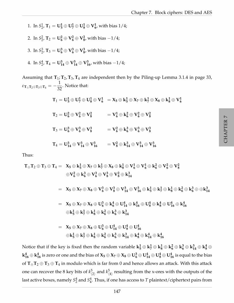
CH

AP

TE

R7

CH

AP

TE

R7

CH

AP

TE

R7

CH

AP

TE

R7

CH

AP

TE

R7

CH

AP

TE

R7


1. In S12, T1 = U1

5 ⊕U17 ⊕U1

8 ⊕V16, with bias 1/4;

2. In S22, T2 = U2

6 ⊕V26 ⊕V2

8, with bias −1/4;

3. In S32, T3 = U3

6 ⊕V36 ⊕V3


4. In S42, T4 = U3

14 ⊕V314 ⊕V3


Assuming that T1; T2, T3, T4 are independent then by the Piling-up Lemma 3.1.4 in page 33,

εT⊕T2⊕T3⊕T4 = −1

32. Notice that:

T1 = U15 ⊕U1

7 ⊕U18 ⊕V1

6 = X5 ⊕ k15 ⊕ X7 ⊕ k1

7 ⊕ X8 ⊕ k18 ⊕V1

6

T2 = U26 ⊕V2

6 ⊕V28 = V1

6 ⊕ k26 ⊕V2

6 ⊕V28

T3 = U36 ⊕V3

6 ⊕V38 = V2

6 ⊕ k36 ⊕V3

6 ⊕V38

T4 = U314 ⊕V3

14 ⊕V316 = V2

8 ⊕ k314 ⊕V3

14 ⊕V316

Thus:

T⊕T2 ⊕ T3 ⊕ T4 = X5 ⊕ k15 ⊕ X7 ⊕ k1

7 ⊕ X8 ⊕ k18 ⊕V1

6 ⊕V16 ⊕ k2

6 ⊕V26 ⊕V2

8

⊕V26 ⊕ k3

6 ⊕V36 ⊕V3

8 ⊕V28 ⊕ k3

14

= X5 ⊕ X7 ⊕ X8 ⊕V36 ⊕V3

8 ⊕V314 ⊕V3

16 ⊕ k15 ⊕ k1

7 ⊕ k18 ⊕ k2

6 ⊕ k36 ⊕⊕k3

14

= X5 ⊕ X7 ⊕ X8 ⊕U36 ⊕ k4

6 ⊕U414 ⊕ k4

16 ⊕U48 ⊕ k4

8 ⊕U416 ⊕ k4

16

⊕k15 ⊕ k1

7 ⊕ k18 ⊕ k2

6 ⊕ k36 ⊕ k3

14

= X5 ⊕ X7 ⊕ X8 ⊕U36 ⊕U4

14 ⊕U48 ⊕U4

16

⊕k15 ⊕ k1

7 ⊕ k18 ⊕ k2

6 ⊕ k36 ⊕ k3

14 ⊕ k48 ⊕ k4

14 ⊕ k416

Notice that if the key is fixed then the random variable k15 ⊕ k1

7 ⊕ k18 ⊕ k2

6 ⊕ k36 ⊕ k3

14 ⊕ k48 ⊕

k416⊕ k4

16 is zero or one and the bias of X5⊕X7⊕X8⊕U36⊕U4

14⊕U48⊕U4

16 is equal to the bias

of T⊕T2 ⊕ T3 ⊕ T4 in modulo which is far from 0 and hence allows an attack. With this attack

one can recover the 8 key bits of k5〈2〉 and k5

〈4〉 resulting from the x-ores with the outputs of the

last active boxes, namely S42 and S4

4. Thus, if one has access to T plaintext/ciphertext pairs from

147

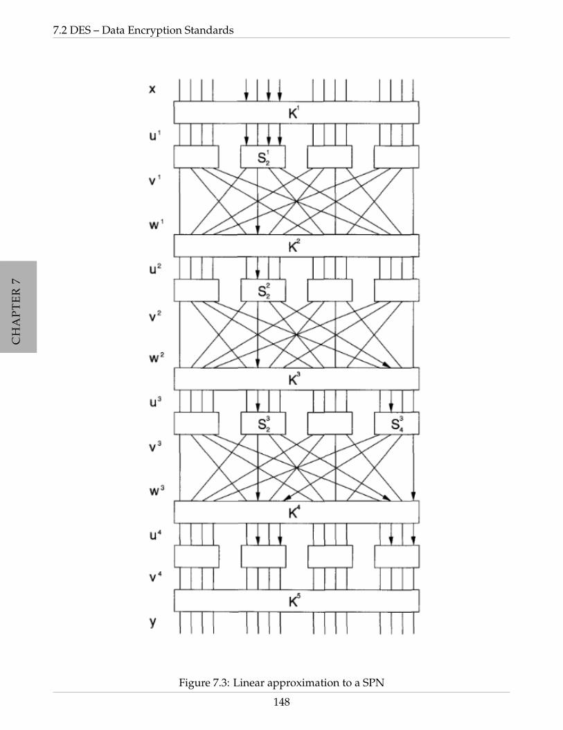
CH

AP

TE

R7

CH

AP

TE

R7

CH

AP

TE

R7

CH

AP

TE

R7

CH

AP

TE

R7

CH

AP

TE

R7


Figure 7.3: Linear approximation to a SPN

148

CH

AP

TE

R7

CH

AP

TE

R7

CH

AP

TE

R7

CH

AP

TE

R7

CH

AP

TE

R7

CH

AP

TE

R7


the partial decryption of the ciphertext y to obtain u4〈2〉 and u4

〈4〉 and hence one can compute the

value x5 ⊕ x7 ⊕ x8 ⊕ u46 ⊕ u4

8 ⊕ u414 ⊕ u4

16. Keeping an array of counters indexed by the 256

possible candidate subkeys, and increment the counter corresponding to a particular subkey

has the value 0 and in the end it is expected that most counters will have a value close to T/2,

but the counter for the correct candidate subkey will have a value that is close to T/2± T/32

which allows the identification of eight subkey bits. These ideas are expressed in the next

algorithm designed for this particular linear attack.

Algorithm 7.2.2 (Linear attack)

Input A number T, a set T of T plaintext/ciphertexts and the inverse of the substitution

permutation π−1.

Output The eight bits of the key.

Step 1 For (L1, L2) from (0, 0) to(F, F) (the number are in hexadecimal base) do :

Step 1.1 Count(L1, L2) = 0;

Step 2 For all (x, y) ∈ T do:

Step 2.1 For (L1, L2) from (0, 0) to(F, F) do:

Step 2.1.1 v4〈2〉 = L1 ⊕ y〈2〉;

Step 2.1.2 v4〈4〉 = L2 ⊕ y〈4〉;

Step 2.1.3 u4〈2〉 = π−1(v4

〈2〉);

Step 2.1.4 u4〈4〉 = π−1(v4

〈4〉);

Step 2.1.5 z = x5 ⊕ x7 ⊕ x8 ⊕ u46 ⊕ u4

8 ⊕ u414 ⊕ u4

16;

Step 2.1.6 If z = 0 then Count(L1, L2) = Count(L1, L2) + 1;

Step 3 max = −1;

Step 4 For (L1, L2) from (0, 0) to(F, F) do :

Step 4.1 Count(L1, L2) = |Count(L1, L2)− T/2|;

149

CH

AP

TE

R7

CH

AP

TE

R7

CH

AP

TE

R7

CH

AP

TE

R7

CH

AP

TE

R7

CH

AP

TE

R7


Step 4.2 If Count(L1, L2) > max then max = Count(L1, L2) and maxkey = (L1, L2).

Step 5 Output (maxkey)

In general, a linear attack based on a linear approximation having bias equal to ε will be

successful if the number of plaintext/ciphertext pairs is approximately cε−2, for some small

constant c.

• • •

7.2.2.2 The differential attack

In this technique (also consisting of plaintext/ciphertext attacks) was developed by Biham and

Shamir in 93 and the basic idea behind it is to keep track of specific differences in the input

that lead to specific differences in the output with noticeable probability when compared with

a random permutation. In a not looking random block cipher there may be differentials that

appear with significantly higher probability and those are the ones that are attackable. So one

will look for those differences via a careful analysis of the block cipher itself. The point of

differential cryptanalysis is to use many differentials, to recover the secret key. Similar to the

linear attack the ability to isolate parts of a key is crucial and enables the attacker to obtain

the key in time less than a brute force search, however, since chosen plaintexts/ciphertexts are

required the practicality of this attack is questionable (but real).

Differential cryptanalysis involves than the comparison of two xor of two inputs with the xor

of their corresponding outputs. Assume that the attacker has access to a large number of tuples

(x, x∗, y, y∗), where x′ = x ⊕ x∗ is a fixed value and all of then are encrypted using the same

unknown key, k. The trick is for each of these tuples, one decrypt the respectively ciphertexts

y and y∗, using all possible candidate keys for the last round of the cipher and analyze the

values of certain state bits, and determine if their x-or has a certain value (namely, the most

likely value for the given input x-or). Whenever it does, the counter for that particular key

incremented. At the end of this process, the candidate key that has the highest frequency count

contains the correct values for these key bits.

150

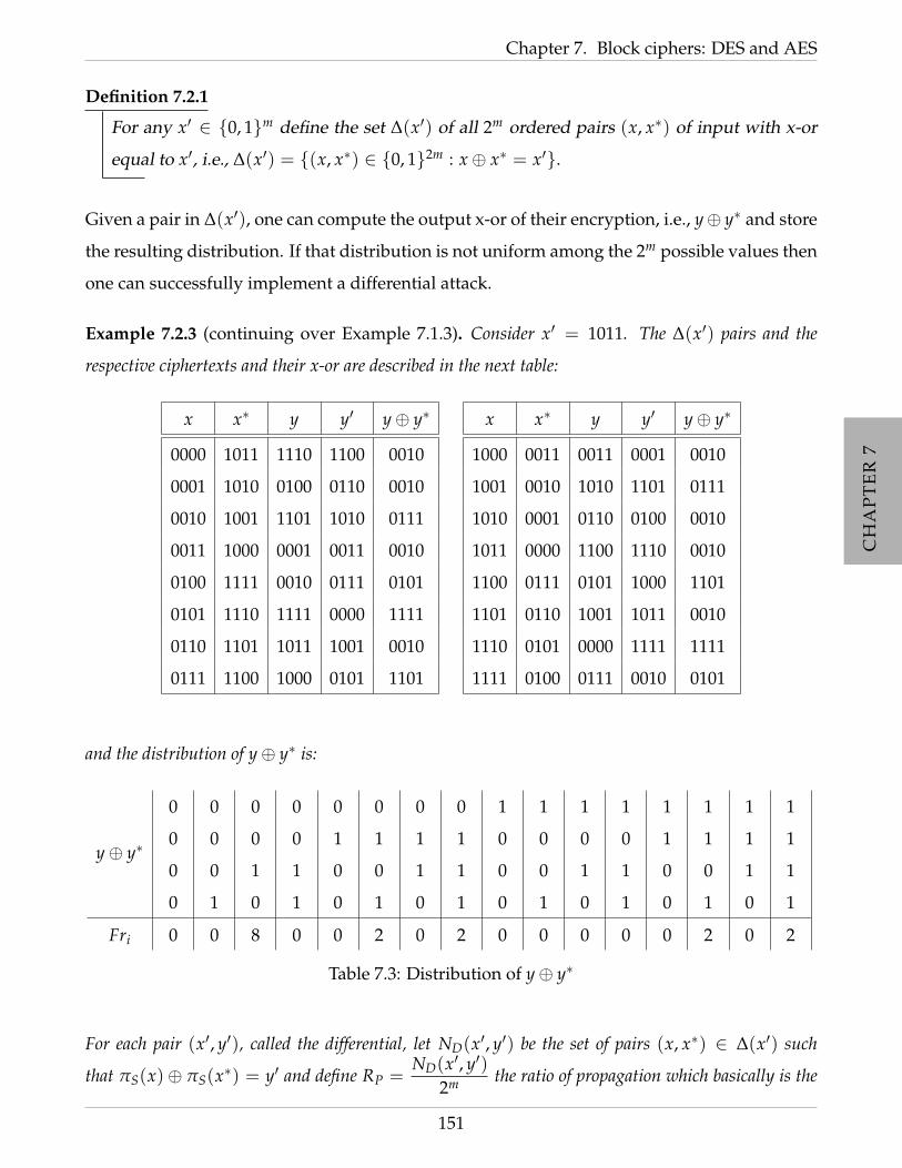
CH

AP

TE

R7

CH

AP

TE

R7

CH

AP

TE

R7

CH

AP

TE

R7

CH

AP

TE

R7

CH

AP

TE

R7


Definition 7.2.1

For any x′ ∈ 0, 1m define the set ∆(x′) of all 2m ordered pairs (x, x∗) of input with x-or

equal to x′, i.e., ∆(x′) = (x, x∗) ∈ 0, 12m : x⊕ x∗ = x′.

Given a pair in ∆(x′), one can compute the output x-or of their encryption, i.e., y⊕ y∗ and store

the resulting distribution. If that distribution is not uniform among the 2m possible values then

one can successfully implement a differential attack.

Example 7.2.3 (continuing over Example 7.1.3). Consider x′ = 1011. The ∆(x′) pairs and the

respective ciphertexts and their x-or are described in the next table:

x x∗ y y′ y⊕ y∗

0000 1011 1110 1100 0010

0001 1010 0100 0110 0010

0010 1001 1101 1010 0111

0011 1000 0001 0011 0010

0100 1111 0010 0111 0101

0101 1110 1111 0000 1111

0110 1101 1011 1001 0010

0111 1100 1000 0101 1101

x x∗ y y′ y⊕ y∗

1000 0011 0011 0001 0010

1001 0010 1010 1101 0111

1010 0001 0110 0100 0010

1011 0000 1100 1110 0010

1100 0111 0101 1000 1101

1101 0110 1001 1011 0010

1110 0101 0000 1111 1111

1111 0100 0111 0010 0101

and the distribution of y⊕ y∗ is:

y⊕ y∗

0

0

0

0

0

0

0

1

0

0

1

0

0

0

1

1

0

1

0

0

0

1

0

1

0

1

1

0

0

1

1

1

1

0

0

0

1

0

0

1

1

0

1

0

1

0

1

1

1

1

0

0

1

1

0

1

1

1

1

0

1

1

1

1

Fri 0 0 8 0 0 2 0 2 0 0 0 0 0 2 0 2

Table 7.3: Distribution of y⊕ y∗

For each pair (x′, y′), called the differential, let ND(x′, y′) be the set of pairs (x, x∗) ∈ ∆(x′) such

that πS(x)⊕ πS(x∗) = y′ and define RP =ND(x′, y′)

2m the ratio of propagation which basically is the

151

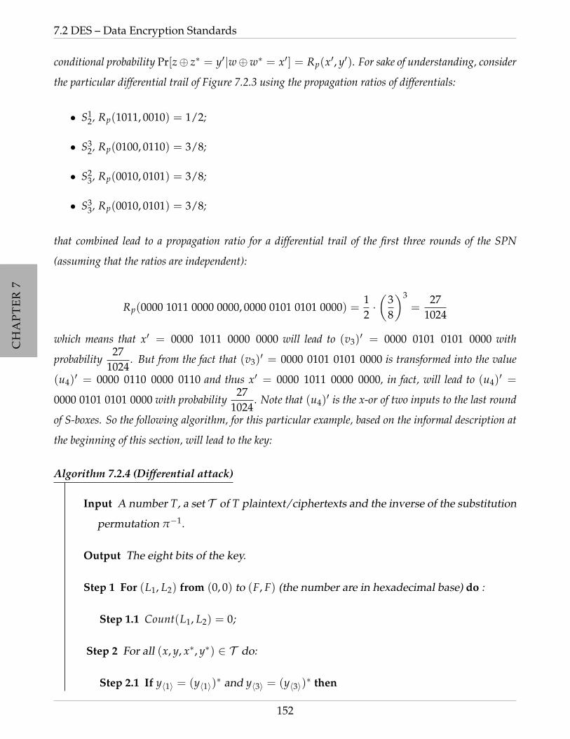
CH

AP

TE

R7

CH

AP

TE

R7

CH

AP

TE

R7

CH

AP

TE

R7

CH

AP

TE

R7

CH

AP

TE

R7


conditional probability Pr[z⊕ z∗ = y′|w⊕w∗ = x′] = Rp(x′, y′). For sake of understanding, consider

the particular differential trail of Figure 7.2.3 using the propagation ratios of differentials:

• S12, Rp(1011, 0010) = 1/2;

• S32, Rp(0100, 0110) = 3/8;

• S23, Rp(0010, 0101) = 3/8;

• S33, Rp(0010, 0101) = 3/8;

that combined lead to a propagation ratio for a differential trail of the first three rounds of the SPN

(assuming that the ratios are independent):

Rp(0000 1011 0000 0000, 0000 0101 0101 0000) =12·(

38

)3

=27

1024

which means that x′ = 0000 1011 0000 0000 will lead to (v3)′ = 0000 0101 0101 0000 with

probability27

1024. But from the fact that (v3)

′ = 0000 0101 0101 0000 is transformed into the value

(u4)′ = 0000 0110 0000 0110 and thus x′ = 0000 1011 0000 0000, in fact, will lead to (u4)

′ =

0000 0101 0101 0000 with probability27

1024. Note that (u4)

′ is the x-or of two inputs to the last round

of S-boxes. So the following algorithm, for this particular example, based on the informal description at

the beginning of this section, will lead to the key:

Algorithm 7.2.4 (Differential attack)

Input A number T, a set T of T plaintext/ciphertexts and the inverse of the substitution

permutation π−1.

Output The eight bits of the key.

Step 1 For (L1, L2) from (0, 0) to (F, F) (the number are in hexadecimal base) do :

Step 1.1 Count(L1, L2) = 0;

Step 2 For all (x, y, x∗, y∗) ∈ T do:

Step 2.1 If y〈1〉 = (y〈1〉)∗ and y〈3〉 = (y〈3〉)∗ then

152

CH

AP

TE

R7

CH

AP

TE

R7

CH

AP

TE

R7

CH

AP

TE

R7

CH

AP

TE

R7

CH

AP

TE

R7


Figure 7.4: Differential attack for a SPN

153

CH

AP

TE

R7

CH

AP

TE

R7

CH

AP

TE

R7

CH

AP

TE

R7

CH

AP

TE

R7

CH

AP

TE

R7


Step 2.2.1 For (L1, L2) from (0, 0) to(F, F) do :

Step 2.2.1.1 v4〈2〉 = L1 ⊕ y〈2〉

Step 2.2.1.2 v4〈4〉 = L2 ⊕ y〈4〉

Step 2.2.1.3 u4〈2〉 = π−1(v4

〈2〉)

Step 2.2.1.4 u4〈4〉 = π−1(v4

〈4〉)

Step 2.2.1.5 (v4〈2〉)∗ = L1 ⊕ (y〈2〉)∗

Step 2.2.1.6 (v4〈4〉)∗ = L2 ⊕ (y〈4〉)∗

Step 2.2.1.7 (u4〈2〉)∗ = π−1(v4

〈2〉)∗

Step 2.2.1.8 (u4〈4〉)∗ = π−1(v4

〈4〉)∗;

Step 2.2.1.9 u4〈2〉)′ = u4

〈2〉 ⊕ (u4〈2〉)∗;

Step 2.2.1.10 (u4〈4〉)′ = u4

〈4〉 ⊕ (u4〈4〉)∗;

Step 2.2 If (u4〈4〉)′ = 0110 and (u4

〈4〉)′ = 0110 then Count(L1, L2) = Count(L1, L2) + 1;

Step 3 max = −1;

Step 4 For (L1, L2) from (0, 0) to(F, F) do :

Step 4.1 If Count(L1, L2) > max then

Step 4.1.1 max = Count(L1, L2);

Step 4.1.2 maxkey = (L1, L2);

Step 5 Output (maxkey)

• • •

7.2.2.3 Analytic attack

To be written

154

CH

AP

TE

R7

CH

AP

TE

R7

CH

AP

TE

R7

CH

AP

TE

R7

CH

AP

TE

R7

CH

AP

TE

R7


• • • • • • • • • • • • • • • • • • • • • • • • • • • • • • • • • • • • •

SECTION 7.3

AES – Advanced Encryption Standards

Since one can ”possibly” break DES with sufficiently large pair of plaintext/ciphertext and

the need of secretly encrypt messages were the main reasons for NIST to began in 1997 the

substitution of DES and that would be called Advanced Encryption Standards (AES) that can

offer a higher level of security. AES candidates were required to:

1. support a symmetric block cipher supporting multiple key lengths (128, 192, 256);

2. have the algorithm publicly available, free to use, and able to run efficiently in both

hardware and software;

3. ensure that the only known approach to decrypt a message is for an intruder to try every

possible key;

There were presented 21 proposals, 15 of them meeting all the necessary criteria that were

announced at the ”First AES Candidate Conference”. In August 1999, five of the candidates

were chosen as finalists: MARS, RC6, Rijndael, Serpent and Twofish. On October 2, 2000,

Rijndael was selected to be the Advanced Encryption Standard and in February 2001, the NIST

published a draft for the AES for public review and comment.

AES was adopted as a standard on November 2001, and it was published as FIPS 197 in the

Federal Register on December 4, 2001.

The great thing about the all process for the AES was it openness and its international feedback

which provided the opportunity for public discussion and analysis of the candidates. The

selected AES, was invented by two Belgian researchers, Daemen and Rijmen.

155

CH

AP

TE

R7

CH

AP

TE

R7

CH

AP

TE

R7

CH

AP

TE

R7

CH

AP

TE

R7

CH

AP

TE

R7

7.3 AES – Advanced Encryption Standards

• • •

7.3.1 Description of AES

AES operates on blocks of size 128 bits and uses a key size of 128, 192, or 256 bits, whereas

Rijndael can be specified with block and key sizes in any multiple of 32 bits, with a minimum

of 128 bits and a maximum of 256 bits.

AES operates on a 4 × 4 array of bytes (i.e., 32 × 32 bits), termed the state and almost all

calculations are done in a special finite field. For each key length the cipher is specified by a

number of repetitions of transformation rounds that convert the input plaintext into the final

output of ciphertext.

Each round consists of several processing steps, including one that depends on the encryption

key. A high level description of the AES is presented in the next algorithm:

Algorithm 7.3.1

Step 1 KeyExpansion

Step 2 Initial round:

Step 2.1 AddRoundKey;

Step 3 Rounds:

Step 3.1 SubBytes;

Step 3.2 ShiftRows;

Step 3.3 MixColumns;


Step 4 Final round:

Step 4.1 SubBytes;

Step 4.2 ShiftRows;


156

CH

AP

TE

R7

CH

AP

TE

R7

CH

AP

TE

R7

CH

AP

TE

R7

CH

AP

TE

R7

CH

AP

TE

R7


Notice that all the operations are important for the security of AES. In fact, the operation

SubBytes achieves non-linearity which is important to prevent differential cryptanalysis, the

operations ShiftRows and MixColumns are used to mix up bits to achieve a more uniform

distribution of ciphertexts and the operation AddRoundKey provides the necessary secret

randomness.

Let x be the plaintext to be ciphered with the AES, consisting of 16 bytes. Usually the content

of a byte will be represented in hexadecimal (in the case composed of two digits). The initial

state S (a word of 16 bytes) is prepared as follows:

s0,0 s0,1 s0,2 s0,3

s1,0 s1,1 s1,2 s1,3

s2,0 s2,1 s2,2 s2,3

s3,0 s3,1 s3,2 s3,3

=

x0 x4 x8 x12

x1 x5 x9 x13

x2 x6 x10 x14

x3 x7 x11 x15

Now it described the process Subbyte which consists of replace each byte by another accord-

ing to the Table 7.4.

So for a byte XY the result is πS(XY) where x is looked in column and Y in the line. Notice

that ΠS contrarily to what happens in DES, it can be represented algebraically. In fact each

byte represents a polynomial in Z2[x]/(x8 + x4 + x3 + x + 1), where the byte a7a6a5a4a3a2a1a0

represents the polynomial p(x) = a7x7 + a6x6 + a5x5 + a4x4 + a3x3 + a2x2 + a1x + a0. The

Subbyte corresponds to invert p(x) in Z2[x]/(x8 + x4 + x3 + x + 1), say q(x) = b7x7 + b6x6 +

b5x5 + b4x4 + b3x3 + b2x2 + b1x + b0 and the coefficients of each of the bits of the result of this

operation say r(x) = c7x7 + c6x6 + c5x5 + c4x4 + c3x3 + c2x2 + c1x + c0 are obtained by the

formula ci = bi + bi+4 + bi+5 + bi+6 + bi+7 + di (mod 2) where d = 01100011.

The ShiftRow is the operation realized by the following diagram:

s′0,0 s′0,1 s′0,2 s′0,3

s′1,0 s′1,1 s′1,2 s′1,3

s′2,0 s′2,1 s′2,2 s′2,3

s′3,0 s′3,1 s′3,2 s′3,3

=

s0,0 s0,1 s0,2 s0,3

s1,1 s1,2 s1,3 s1,0

s2,2 s2,3 s2,0 s2,1

s3,3 s3,0 s3,1 s3,2

157

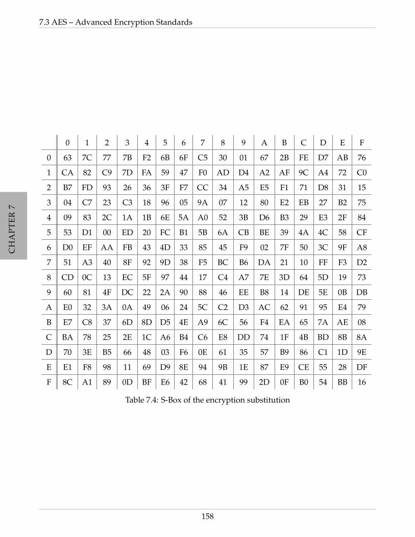
CH

AP

TE

R7

CH

AP

TE

R7

CH

AP

TE

R7

CH

AP

TE

R7

CH

AP

TE

R7

CH

AP

TE

R7

7.3 AES – Advanced Encryption Standards

0 1 2 3 4 5 6 7 8 9 A B C D E F

0 63 7C 77 7B F2 6B 6F C5 30 01 67 2B FE D7 AB 76

1 CA 82 C9 7D FA 59 47 F0 AD D4 A2 AF 9C A4 72 C0

2 B7 FD 93 26 36 3F F7 CC 34 A5 E5 F1 71 D8 31 15

3 04 C7 23 C3 18 96 05 9A 07 12 80 E2 EB 27 B2 75

4 09 83 2C 1A 1B 6E 5A A0 52 3B D6 B3 29 E3 2F 84

5 53 D1 00 ED 20 FC B1 5B 6A CB BE 39 4A 4C 58 CF

6 D0 EF AA FB 43 4D 33 85 45 F9 02 7F 50 3C 9F A8

7 51 A3 40 8F 92 9D 38 F5 BC B6 DA 21 10 FF F3 D2

8 CD 0C 13 EC 5F 97 44 17 C4 A7 7E 3D 64 5D 19 73

9 60 81 4F DC 22 2A 90 88 46 EE B8 14 DE 5E 0B DB

A E0 32 3A 0A 49 06 24 5C C2 D3 AC 62 91 95 E4 79

B E7 C8 37 6D 8D D5 4E A9 6C 56 F4 EA 65 7A AE 08

C BA 78 25 2E 1C A6 B4 C6 E8 DD 74 1F 4B BD 8B 8A

D 70 3E B5 66 48 03 F6 0E 61 35 57 B9 86 C1 1D 9E

E E1 F8 98 11 69 D9 8E 94 9B 1E 87 E9 CE 55 28 DF

F 8C A1 89 0D BF E6 42 68 41 99 2D 0F B0 54 BB 16

Table 7.4: S-Box of the encryption substitution

158

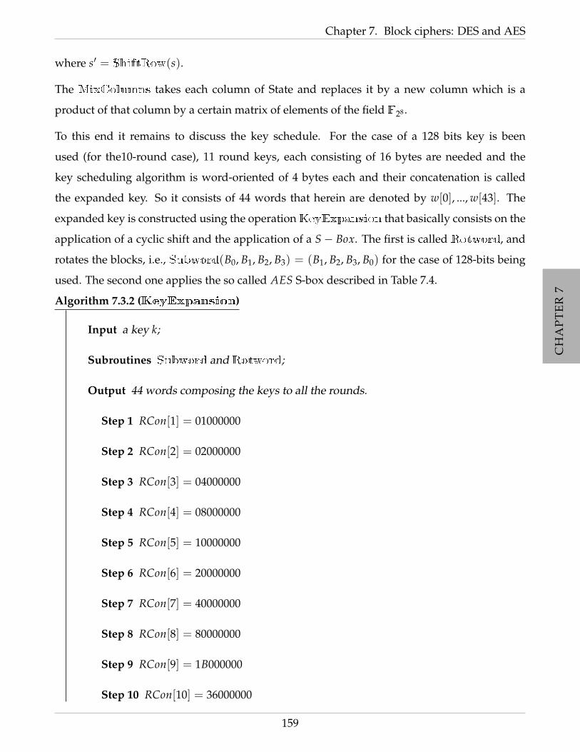
CH

AP

TE

R7

CH

AP

TE

R7

CH

AP

TE

R7

CH

AP

TE

R7

CH

AP

TE

R7

CH

AP

TE

R7


where s′ = ShiftRow(s).

The MixColumns takes each column of State and replaces it by a new column which is a

product of that column by a certain matrix of elements of the field F28 .

To this end it remains to discuss the key schedule. For the case of a 128 bits key is been

used (for the10-round case), 11 round keys, each consisting of 16 bytes are needed and the

key scheduling algorithm is word-oriented of 4 bytes each and their concatenation is called

the expanded key. So it consists of 44 words that herein are denoted by w[0], ..., w[43]. The

expanded key is constructed using the operationKeyExpansion that basically consists on the

application of a cyclic shift and the application of a S− Box. The first is called Rotword, and

rotates the blocks, i.e., Subword(B0, B1, B2, B3) = (B1, B2, B3, B0) for the case of 128-bits being

used. The second one applies the so called AES S-box described in Table 7.4.

Algorithm 7.3.2 (KeyExpansion)

Input a key k;

Subroutines Subword and Rotword;

Output 44 words composing the keys to all the rounds.

Step 1 RCon[1] = 01000000

Step 2 RCon[2] = 02000000

Step 3 RCon[3] = 04000000

Step 4 RCon[4] = 08000000

Step 5 RCon[5] = 10000000

Step 6 RCon[6] = 20000000

Step 7 RCon[7] = 40000000

Step 8 RCon[8] = 80000000

Step 9 RCon[9] = 1B000000

Step 10 RCon[10] = 36000000

159

CH

AP

TE

R7

CH

AP

TE

R7

CH

AP

TE

R7

CH

AP

TE

R7

CH

AP

TE

R7

CH

AP

TE

R7

7.4 Exercises

Step 11 For i = 0 to3 do :

Step 11.1 w[i] = (k[4i], k[4i + 1], k[4i + 2], k[4i + 3])

Step 12 For i = 4 to53 do :

Step 12.1 aux = w[i− 1]

Step 12.2 If i ≡ 0 (mod 4) then

aux = Subword(Rotword(temp))⊕ RCon[i/4];

Step 12.2 w[i] = w[i− 4]⊕ aux

Step 13 Output (w[0], · · · , w[43])

• • • • • • • • • • • • • • • • • • • • • • • • • • • • • • • • • • • • •

SECTION 7.4

Exercises

Exercise 7.4.1 (exercise 5.5 of [KL07]). Consider a Feistel network defined above. Envisage the output

of an r-round when the input is (L0, R0) in each of the following two cases:

1. Each round function outputs all 0’s, regardless of the input.

2. Each round function is the identity function.

Exercise 7.4.2. Consider a DES encryption scheme with the following modification.

Let g : 0, 164 → 0, 132 and each round key ki is defined by g(ki) and modify the round

function f to f (Ri−1; ki) = Ri−1 ⊕ ki.

Describe the output L16 and R16 of given input L0 and R0.

Exercise 7.4.3. Prove that if two vectors words w1 and w2 of four bytes differ in just one byte, then

their images under MixColumns differ in all four bytes.

Exercise 7.4.4. Assume that a cipher block chaining mode as defined in the Algorithm 5.2.2 on Page 95

160

CH

AP

TE

R7

CH

AP

TE

R7

CH

AP

TE

R7

CH

AP

TE

R7

CH

AP

TE

R7

CH

AP

TE

R7


is use in DES. For i = 1, 2, 3, · · · , the encryption rule for a plaintext Pi, key k and a ciphertext Ci−1 is

Ci = DES(Pi ⊕ Ci−1, k)

where C0 is an initial block.

Compute the decryption rule. Suppose that an opponent changes Ci to a different C′i . How many

messages are then decrypted incorrectly?

Exercise 7.4.5 (exercise 3.5 of [Sti06]). Assume that the following 128-bit AES key is given in hex-

adecimal notation:

2B7E151628AED2A6ABF7158809CF4F3C

Construct the complete key schedule arising from this key.

161

CH

AP

TE

R7

CH

AP

TE

R7

CH

AP

TE

R7

CH

AP

TE

R7

CH

AP

TE

R7

CH

AP

TE

R7

7.4 Exercises

162

CH

AP

TE

R7

CH

AP

TE

R7

CH

AP

TE

R7

CH

AP

TE

R7

CH

AP

TE

R7

CH

AP

TE

R7

Part III

The Public Key Cryptography

163

CH

AP

TE

R7

CH

AP

TE

R7

CH

AP

TE

R7

CH

AP

TE

R7

CH

AP

TE

R7

CH

AP

TE

R7

CH

AP

TE

R8

CH

AP

TE

R8

CH

AP

TE

R8

CH

AP

TE

R8

CH

AP

TE

R8

CH

AP

TE

R8

CH

AP

TE

R8

CHAPTER 8

The story behind Public Key

Cryptography

This part of cryptography was only considered very recently and for that reason its history is

short but very fruitful on the impact on the real life.

In previous part of this redaction only cryptographic schemes that demand a private previous

communication between the parties to agree on the key that would be used to encrypt and also

to decrypt the messages exchanged were considered. This particular type of schemes can be

perfectly secure as was previously proved but, fundamentally, these two constrains are severe

drawbacks on the applicability of these schemes on daily use. The introduction of public-key

encryption is one of the milestones that complete changed the course of cryptography as every

one saw it before and how every one sees it now after the introduction of these techniques.

To give a general panorama of what public key cryptography is all about consider the following

example:

Example 8.0.6. Assume that it is impossible for A and B to meet, and that they are therefore unable

to exchange the key in order to communicate privately using a symmetric cryptographic system. In

particular, A and B cannot agree on the key to use since that would have to be plaintext and their

supposedly secret key would be exposed. But A and B can do the following:

B selects both an encryption function and a corresponding decryption function that are not symmetric

165

CH

AP

TE

R8

CH

AP

TE

R8

CH

AP

TE

R8

CH

AP

TE

R8

CH

AP

TE

R8

CH

AP

TE

R8

CH

AP

TE

R8

(i.e., knowing the encryption process does not convey any information about the decryption process,

usually based on an one-way function defined in Section 4.3). Then B sends only the encryption

function to A that uses it to encrypt the message. Notice that even A, once message is encrypted,

cannot decrypt the it. After the encryption in done, A sends the ciphertext to B, who is the only one

able to decrypt it since it has the decryption function. Even if O, the malicious opponent intercepted

B message and learned the encryption function, it is in the same position as A, i.e., knowing both the

encryption function and the encrypted message, it remains unable to decrypt it in feasible time.

Public-key cryptographic schemes were designed to achieve two practical issues: enable the

parties to communicate privately without having to agree on any secret information in advance

and without meeting personally and secondly enable every one to communicate with each

other without to have to for each person that one wishes to communicate a different key. The

latter one is clear for the reader to be unpractical in large scale as one would have to keep a

huge database of keys that would be difficult to manage, specially for the ones that do not

have the knowledge to do it. Notice that in practical terms and specially based on the reader

use of internet, anyone can have a secret (only one) password, for example. For the former

one, the reader that is not familiar with this theory it can be surprising that such thing can

be possible but a simple example can help the reader to understand the basic idea of public

key cryptographic schemes. Imagine that two people in different parts of the globe want

to communicate over the internet and share no initial secret and all that travels around the

internet is public but they want to keep the message secret in such a way that no one else can

learn anything about what they are saying! One way of doing this is just A to send B encrypted

message that used the public part of the key of B and then if the system is secure and the only

way to recover the message is to know the private key of B which is assumed to be untraceable

form the public key. This simple solution is only possible if some conditions are verified. Notice

that in this cases one cannot use symmetric key schemes, since if the public was equal or easily

computable from the private key than no secret would be possible to be shared in this scenario.

It is then mandatory to have, even if somehow related, to have two different keys to encrypt

and decrypt processes.

The public key cryptography, also known as modern cryptography, had born in the decade of

70s of the last century when, mainly the two issues discussed above, were realized and became

166

CH

AP

TE

R8

CH

AP

TE

R8

CH

AP

TE

R8

CH

AP

TE

R8

CH

AP

TE

R8

CH

AP

TE

R8

CH

AP

TE

R8

Chapter 8. The story behind Public Key Cryptography

impossible to have for each pair of users a pair of strings. Although the main impulse for

public key cryptography came from military and commercial use rather than particular parties

A and B. Similar to the described issue discussed above, the task of military encryption key

management had greatly expanded with the growth in electronic communications networks,

and the number of parties that needed to communicate to organize a large-scale military op-

eration such as World War II. In this practical experience communications showed that much

of the messages had ended up unencrypted because there was no time to establish a secure

connection to transmit the agreed key. In the commercial domain the problem impulsed the

public key cryptography since the quickly growing, with increasing use of electronic networks

to conduct sensitive business communications and financial transactions, often between par-

ties from different organizations that had not previously communicated or had the chance to

exchange encryption keys beforehand.

The advent of Cryptography is due to several authors, for example, Ellis and Markle that later

joint Diffie and Hellman who were responsible for putting together the ideas underlying the

public key cryptography and Rivest, Shamir and Adleman there were responsible for the key

transport and digital signing schemes called the RSA system in 1977. Seven years later another

name marked the public key cryptographic system, namely Elgammal, that designed another

system based on elliptic curves and on the Diffie–Hellman key exchange.

All these schemes and many other that were developed insure its security on assumptions on

the hardness of some problems like the discrete logarithm problem or the integer factorization

problem since they, in fact, are not perfectly secure. But just the problems themselves are not

sufficient to guarantee sufficient security and a careful protocol design and a methodology

for defining precisely the security objective and proving that a protocol met that objective are

required. The first step in that direction is to imagine the most powerful adversary possible and

to assign to that adversary a goal or set of goals as weak as possible. In this scenario a protocol

could be deemed secure if an ultra-potent adversary could not achieve his or her ultra-weak

goals and here is where provable security appears in the form of computational assumptions.

Only in middle of 90s provably secure protocols began to be efficient enough to be used in the

real-world.

In the last decades since the appearing of public key cryptography many applications have

167

CH

AP

TE

R8

CH

AP

TE

R8

CH

AP

TE

R8

CH

AP

TE

R8

CH

AP

TE

R8

CH

AP

TE

R8

CH

AP

TE

R8

8.1 Describing a public key cryptographic system

been developed to different purposes that will be discussed in detail in due course of this Part

of this work.

• • • • • • • • • • • • • • • • • • • • • • • • • • • • • • • • • • • • •

SECTION 8.1

Describing a public key cryptographic system

In the previous part where symmetric cryptographic systems were described. The term sym-

metric was used to describe the real symmetry of the encryption and the decryption processes.

In fact, the two processes are very similar since the decryption process can be easily derived

from the encryption process. For example, in the case of substitution scheme described in the

Cryptographic System 5.1.3 the process of decryption is essentially equal to the encryption

process but instead of using the permutation π one uses its inverse. Also, another name that is

commonly use to these schemes are “shared keys” cryptographic systems, since the two parties

involved use the same private key to both encrypt and decrypt information.

As was mentioned before, the symmetric cryptographic schemes have some advantageous and

some disadvantages. The use of the same key for both decryption and encryption makes the

process of encryption and decryption of the messages much faster, it is easier to implement

and also, in general, requires less processing power than public key cryptography that will

be discussed in next paragraphs ahead. The disadvantages of symmetric key cryptography is

that the two parties sending messages to each other must agree to use the same private key

before they start transmitting secure information which might be impossible depending on

the circumstances. The advantage of public key cryptography is that the public key used for

encryption does not need to be kept secret, and that the reason to call these schemes “public”.

Usually, when two parties want to communicate they take advantage of two worlds. They use

public key cryptography to create a shared session key that they keep secret and then they com-

municate through symmetric key cryptography using the shared session key. This way they

can get the best of both worlds – the performance/speed of shared key cryptography along

with the convenience of public key cryptography to avoid meeting personally of expensive

secure channels of communications.

From the discussion above one concludes that the public key cryptography is a system that

168

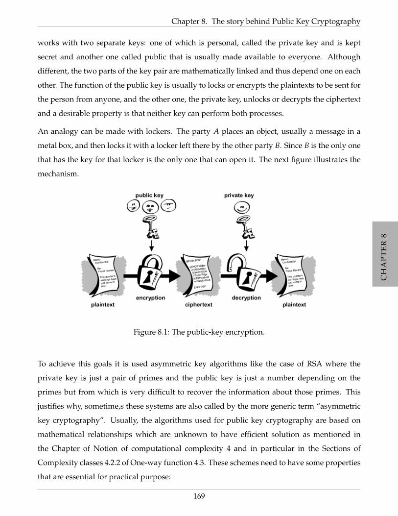
CH

AP

TE

R8

CH

AP

TE

R8

CH

AP

TE

R8

CH

AP

TE

R8

CH

AP

TE

R8

CH

AP

TE

R8

CH

AP

TE

R8


works with two separate keys: one of which is personal, called the private key and is kept

secret and another one called public that is usually made available to everyone. Although

different, the two parts of the key pair are mathematically linked and thus depend one on each

other. The function of the public key is usually to locks or encrypts the plaintexts to be sent for

the person from anyone, and the other one, the private key, unlocks or decrypts the ciphertext

and a desirable property is that neither key can perform both processes.

An analogy can be made with lockers. The party A places an object, usually a message in a

metal box, and then locks it with a locker left there by the other party B. Since B is the only one

that has the key for that locker is the only one that can open it. The next figure illustrates the

mechanism.

Figure 8.1: The public-key encryption.

To achieve this goals it is used asymmetric key algorithms like the case of RSA where the

private key is just a pair of primes and the public key is just a number depending on the

primes but from which is very difficult to recover the information about those primes. This

justifies why, sometime,s these systems are also called by the more generic term “asymmetric

key cryptography”. Usually, the algorithms used for public key cryptography are based on

mathematical relationships which are unknown to have efficient solution as mentioned in

the Chapter of Notion of computational complexity 4 and in particular in the Sections of

Complexity classes 4.2.2 of One-way function 4.3. These schemes need to have some properties

that are essential for practical purpose:

169

CH

AP

TE

R8

CH

AP

TE

R8

CH

AP

TE

R8

CH

AP

TE

R8

CH

AP

TE

R8

CH

AP

TE

R8

CH

AP

TE

R8


• The production of public and private keys is computationally easy;

• Decrypting a message using the private key is feasible;

• Encrypting a message using the public key is also feasible;

• Anyone trying to derive the private key using the information that is publicly available,

in the case the public key, for example is unfeasible and computational hard.

Notice that item 2 and item 4 above remind the concept of trapdoor one-way function pre-

sented in Definition 4.3.3 on page 4.3.3 since without the knowledge of the private key, com-

puting the plaintext of a message is hard, but with the use of the private key that computation

becomes trivial to achieve.

Unlike symmetric key algorithms, the public key algorithms do not require a secure initial

exchange of one (or more) secret keys between the sender and receiver and, as an extra fea-

ture, they can also be used to authenticate a message by creating a digital signature of the

message using the private key, which can then be verified by using the public key. The most

common uses of the public key systems are the public key distribution systems, the digital

signature systems, and the public key cryptographic systems, which can perform both public

key distribution and digital signature services. In wikipedia some clever and very elucidative

parallel situations explaining these concepts are presented (complementary to the analogy

made above):

An analogy to public-key encryption is that of a locked mail box with a mail

slot. The mail slot is exposed and accessible to the public – its location (the street

address) is, in essence, the public key. Anyone knowing the street address can

go to the door and drop a written message through the slot. However, only the

person who possesses the key can open the mailbox and read the message.

An analogy for digital signatures is the sealing of an envelope with a personal

wax seal. The message can be opened by anyone, but the presence of the unique

seal authenticates the sender.

in wikipedia

170

CH

AP

TE

R8

CH

AP

TE

R8

CH

AP

TE

R8

CH

AP

TE

R8

CH

AP

TE

R8

CH

AP

TE

R8

CH

AP

TE

R8


The basic work of a public key cryptographic system is the following. The party A widely dis-

seminates its public key that will work as the encrypting-key and keeps private the decrypting-

key. B, to encrypt a message to A encrypts with A public key. After receiving the message A

uses the private key to decode the message sent by B.

Next it is presented formally the concept of public key Cryptographic system which will be use

in the rest of these notes.

Definition 8.1.1 (Public key cryptographic system)

A public key cryptographic system is a tuple PKC = (P, C, K, E, D, R, r) where:

1. P is the set of plaintexts;

2. C is the set of ciphertexts;

3. K is the set of keys;

4. R is the part of the key that is made public (which is revealed);

5. r : K → R is called the revealing or the publication function and is a polynomial time

computable function.

6. E consists of encrypting one-way functions with trapdoor k (accordingly to Definition

4.3.3) using the part of the key that is public, i.e., consists of functions er : P → C that

are trapdoor one way functions and where r ∈ R, which, of course depends on a key

k ∈ K such that u(k) = r (k is trapdoor).

7. D consists of decrypting functions dk : C → P, such that dk(er(k)) = x.

171

CH

AP

TE

R8

CH

AP

TE

R8

CH

AP

TE

R8

CH

AP

TE

R8

CH

AP

TE

R8

CH

AP

TE

R8

CH

AP

TE

R8


172

CH

AP

TE

R9

CH

AP

TE

R9

CH

AP

TE

R9

CH

AP

TE

R9

CH

AP

TE

R9

CH

AP

TE

R9

CH

AP

TE

R9

CH

AP

TE

R9

CHAPTER 9

The RSA cryptographic system

The RSA is, as the reader might know or at least have an idea, an algorithm of public-key

cryptography that is based on the presumed difficulty of factoring problem. The name RSA

is due to its own designers, Ron Rivest, Adi Shamir and Leonard Adleman, who first publicly

described it in 1977. It is worth mentioning that in 1973, Clifford Cocks, an English mathemati-

cian, working for the Communication Electronics Security Group (CESG), a special section of

the British Government Communications Headquarters (GCHQ) had developed an equivalent

system in 1973, but its design was kept secret and classified until 1997.

An A user of RSA creates and then publishes the product of two large prime numbers, along

with an auxiliary value, as their public key. The prime factors must be kept secret, otherwise

one could use them to perform the decryption process with acknowledgment of the interested

party. Anyone can use the public key to encrypt a message, but with currently published

methods, if the public key is large enough, only someone with knowledge of factorization of

the number can feasibly decode the message. Whether breaking RSA encryption is as hard as

factoring is an open question known as the RSA problem.

To properly present the RSA cryptographic system one needs to explain several issues con-

cerning the practical implementation of RSA. For example, one needs to justify why one can

perform modular exponentiation of find the inverse of a umber modulo an integer in polyno-

mial time.

173

CH

AP

TE

R9

CH

AP

TE

R9

CH

AP

TE

R9

CH

AP

TE

R9

CH

AP

TE

R9

CH

AP

TE

R9

CH

AP

TE

R9

CH

AP

TE

R9

9.1 The RSA cryptographic system

In Section 2.3 of Chapter 2 it was already proved that (Zn,+,×) is a ring and also that b ∈ Zn

admits inverse if and only if gcd(n, b) = 1.

• • • • • • • • • • • • • • • • • • • • • • • • • • • • • • • • • • • • •

SECTION 9.1

The RSA cryptographic system

Now it is possible to describe the RSA Cryptographic system formally. The RSA is performed

over Zn where n is the product of two distinct odd primes p and q. Notice that, in this case one

has φ(n) = (p− 1)(q− 1), where φ(n) in the value of Euler’s function on n, i.e., the number of

natural numbers less of equal to n that are co-prime with n.

Cryptographic system 9.1.1 (RSA cipher system)

The RSA cipher system is a tupleRSA = (P, C, K, E, D, R, r) where:

1. P = C = Zn, where n = p× q for primes p and q;

2. K consists of pairs k = (a, b) ∈ (Zn)2 such that a · b ≡ 1 (mod φ(n)), i.e., a and b are

inverse of each order modulo φ(n) where φ(n) is the n’s value of Euler’s function;

3. R = Zn;

4. Given a pair (a, b), r(a, b) = b;

5. For each k = (a, b) ∈ K and all x, y ∈ Zn, ek(x) = xb (mod n) and dk(y) = ya

(mod n).

6. The values n and b form the public key, and p, q, a are the private key.

The first step is to prove that in fact the cryptographic system described above is indeed in

conditions of Definition of public cryptographic system presented in 8.1.1 on Page 171 in the

sense that decrypting an encrypted text leads to the original text.

Theorem 9.1.1

Let k, n, p, q, a and b be as defined above in the RSA cipher system. Then for all x ∈ Zn,

dk(ek(x)) = x.

174

CH

AP

TE

R9

CH

AP

TE

R9

CH

AP

TE

R9

CH

AP

TE

R9

CH

AP

TE

R9

CH

AP

TE

R9

CH

AP

TE

R9

CH

AP

TE

R9

Chapter 9. The RSA cryptographic system

Proof: From the fact that a · b ≡ 1 (mod φ(n)), it follows that φ(n)|(ab − 1) and thus, there

exists c ∈ Z such that cφ(n) = ab− 1⇔ ab = cφ(n) + 1. Then:

dk(ek(x)) = (xb)a (mod n)

≡ xba (mod n)

≡ xcφ(n)+1 (mod n)

If x ∈ Z∗n then xcφ(n)+1 (mod n) = (xφ(n))cx (mod n) ≡ x (mod n) directly by Euler’s Theo-

rem 2.3.6 on Page 23.

If x ∈ Zn −Z∗n then one needs to use the Chinese Remainder Theorem 2.3.4 on Page 22.

Since x ∈ Zn − Z∗n, then either p or q is a common divisor of x and n. Assume without loss

generality that q|x. Then

x ≡ 0 (mod q)⇔

xcφ(n)+1 ≡ 0 (mod q)⇔

xcφ(n)+1 ≡ x (mod q)

Also, since x < n and q|x then p 6 |x and thus

xcφ(n)+1 (mod p) ≡ (xc(q−1))(p−1) · x (mod p)

≡ 1 · x (mod p)

by Fermat’s Little Theorem 2.3.5 on page 22. So, by the Chinese Remainder Theorem 2.3.4, one

concludes that x is unique such that

xcφ(n)+1 (mod n) ≡ x (mod n).

Example 9.1.2. To encrypt a message with the encryption scheme of RSA, each letter of the alphabet is

transformed into a number.

175

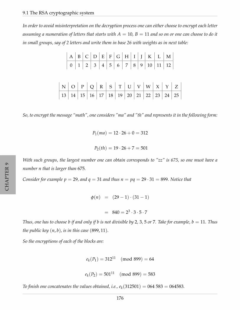
CH

AP

TE

R9

CH

AP

TE

R9

CH

AP

TE

R9

CH

AP

TE

R9

CH

AP

TE

R9

CH

AP

TE

R9

CH

AP

TE

R9

CH

AP

TE

R9

9.1 The RSA cryptographic system

In order to avoid misinterpretation on the decryption process one can either choose to encrypt each letter

assuming a numeration of letters that starts with A = 10, B = 11 and so on or one can choose to do it

in small groups, say of 2 letters and write them in base 26 with weights as in next table:

A B C D E F G H I J K L M

0 1 2 3 4 5 6 7 8 9 10 11 12

N O P Q R S T U V W X Y Z

13 14 15 16 17 18 19 20 21 22 23 24 25

So, to encrypt the message “math”, one considers ”ma” and ”th” and represents it in the following form:

P1(ma) = 12 · 26 + 0 = 312

P2(th) = 19 · 26 + 7 = 501

With such groups, the largest number one can obtain corresponds to ”zz” is 675, so one must have a

number n that is larger than 675.

Consider for example p = 29, and q = 31 and thus n = pq = 29 · 31 = 899. Notice that

φ(n) = (29− 1) · (31− 1)

= 840 = 23 · 3 · 5 · 7

Thus, one has to choose b if and only if b is not divisible by 2, 3, 5 or 7. Take for example, b = 11. Thus

the public key (n, b), is in this case (899, 11).

So the encryptions of each of the blocks are:

ek(P1) = 31211 (mod 899) = 64

ek(P2) = 50111 (mod 899) = 583

To finish one concatenates the values obtained, i.e., ek(312501) = 064 583 = 064583.

176

CH

AP

TE

R9

CH

AP

TE

R9

CH

AP

TE

R9

CH

AP

TE

R9

CH

AP

TE

R9

CH

AP

TE

R9

CH

AP

TE

R9

CH

AP

TE

R9


To decrypt one considers the inverse of b modulo φ(899) i.e., a = bφ(φ(n))−1 (mod 840) = 11288−1

(mod 840) = 611. In particular, to decode 064583 one brakes again into blocks

T1 = 064 P2 = 583

dk(T1) = 64611 (mod 899) = 312

dk(T2) = 191257 (mod 899) = 501

Notice that all together the message needs to have a even number of elements. So, the deciphered message

is dk(064583) = 312 501 = 312501 which is decoded by “math” reserving the calculations in base 26.

In practice the numbers used in the RSA cryptographic system are very large, usually with size

in the order of 1024 bits, i.e., with more than 300 decimal digits. This is a precaution against

the fastest computers that with these kind of numbers are useless simple they would require

more than universe time to factor it. One example is

n = 119294134840169509055527211331255649644606569661527638

012067481954943056851150333806315957037715620297305000

118628770846689969112892212245457118060574995989517080

042105263427376322274266393116193517839570773505632231

596681121927337473973220312512599061231322250945506260

066557538238517575390621262940383913963

This is composed of the two primes

p = 093376618363257581761151703473066828715579998463222345

413874567112127345628767000829084330287552127497024531

4593222946129064538358581018615539828479146469

and

q = 109106169673491102317237340786149226453370608821417489

682098342251389760111799933942998101597369044685540217

08289824396553412180514827996444845438176099727

177

CH

AP

TE

R9

CH

AP

TE

R9

CH

AP

TE

R9

CH

AP

TE

R9

CH

AP

TE

R9

CH

AP

TE

R9

CH

AP

TE

R9

CH

AP

TE

R9

9.2 Euclidean Algorithm for the gcd and the modular exponentiation

Notice that, in theory, the encryption scheme of RSA described in the Cryptographic system

9.1.1 on Page 174 works perfectly but in order to be a cipher scheme that can be used in

practice one must so that its operations are computable in polynomial time (like the modular

exponentiation and the determination of the greatest common divisor) and preferably has some

security properties. Notice that, one needs the Euclidean algorithm to run in polynomial time

to establish the public key and the modular exponentiation to determine the inverse of the

public key modulo φ(n) to establish a private key.

The practical implementation is discussed in the next section and the security issues in the

subsequent ones.

• • • • • • • • • • • • • • • • • • • • • • • • • • • • • • • • • • • • •

SECTION 9.2

Euclidean Algorithm for the gcd and the modular

exponentiation

In Chapter 2 it was already presented the modular algebras and some classical results concern-

ing the elements ofZn andZ∗n. One fundamental property that is used in the RSA is the fact that

(Z∗n,+,×) is a field, and in particular, any element of Z∗n has inverse. For practical purposes

of implementation of RSA, it is crucial the Euclidean algorithm to ensure, for example, that

one can determine the public key as mentioned above since, as it will be seen in this section,

one can determine the greatest common divisor of two numbers efficiently and thus establish

a public key properly in a reasonable time.

Algorithm 9.2.1 (Euclidean Algorithm)

For simplicity call it Euclides(a, b)

Input: Two natural numbers a and b.

Output: gcd(a, b) the greatest common divisor between a and b.

Step 1: If b = 0 then Output a else

Step 1.2: Output Euclides(b, a (mod b)).

178

CH

AP

TE

R9

CH

AP

TE

R9

CH

AP

TE

R9

CH

AP

TE

R9

CH

AP

TE

R9

CH

AP

TE

R9

CH

AP

TE

R9

CH

AP

TE

R9


Theorem 9.2.1 (Lame Theorem)

If a and b be natural numbers such that a > b ≥ 0 and Euclides(a, b) has k ≥ 1 recursive

calls then a ≥ Fk+2 and b ≥ Fk+1, where F is the Fibonacci sequence.

Proof: The proof is carried out by induction over k.

(Base k = 1)

Assume by reduction to absurd that a < F3 = 2 or b < F2 = 1.

In the latter case if b < 1 then b = 0 and thus Euclides(a, b) does not perform any recursive

call and thus k = 0 which contradicts k = 1.

In the former case, since a < 2 and b < a then a = 1 and b = 0 and by the same reason one

concludes that is absurd.

Thus a ≥ F3 and b ≥ F2.

(Step k + 1)

Assume that the algorithm Euclides(a, b) performs k + 1 recursive calls. It is easy to see that

Euclides(a, b) = Euclides(b, a (mod b)) and b + a (mod b) ≤ a. Thus, the number of re-

cursive calls of the algorithm Euclides(a, b) is equal to the recursive calls of 1+Euclides(b, a

(mod b)), i.e, Euclides(b, a (mod b)) uses k recursive calls. Hence, by induction hypothesis:

b ≥ Fk+2

a (mod b) ≥ Fk+1

Since b ≥ Fk+2, to this end, it remains to show that a ≥ Fk+3. Since a ≥ b + a (mod b) ≥

Fk+2 +Fk+1 = Fk+3.

Corollary 9.2.2. If a and b be natural numbers such that a > b ≥ 0 and b ≤ Fk+1, then there are at

mot k recursive calls in Euclides(a, b)

Notice that Fk <Φk√

5≤ Φk, where Φ =

1 +√

52

is the golden ration. Thus, if b ≥ Fk, then the

number of recursive calls of Euclides(a, b) is at most logΦ(b) ∈ O(log(k). This observations

lead to the following result:

179

CH

AP

TE

R9

CH

AP

TE

R9

CH

AP

TE

R9

CH

AP

TE

R9

CH

AP

TE

R9

CH

AP

TE

R9

CH

AP

TE

R9

CH

AP

TE

R9


Theorem 9.2.2

Let a, b and n be natural numbers such b ≤ a ≤ n. Thus, Time(Euclides(a, b)) ≤ O(log3 n).

Proof: By Lamne Theorem 9.2.1 proved above on Page 179, there are at most O(log n) recur-

sive calls of Euclides(a, b). Notice that the last call costs c log n, (just one comparison), the

penultimate costs 2c log n (one comparison and the last recursive call) and so on. Thus:

Time(Euclides(a, b)) ≤c log n

∑i=1

i · c log n · c log n · (log n)2 ∈ O(log3 n).

One can generalize the Euclidean algorithm to the one that retrieves also the inverse modulo

n. This algorithm is called the Extended Euclidean Algorithm.

Algorithm 9.2.3 (Extended Euclidean Algorithm)

For simplicity call it ExtentedEuclides(a, b)

Input: Two natural numbers a and b greater or equal to 1.

Output: gcd(a, b) the greatest common divisor between a and b and the coefficients of

the linear combination witnessing the gcd(a, b).

Step 1: If b = 0 then Output (a, 1, 0) else

Step 2.1: (r′, s′, t′) = ExtentedEuclides(b, a (mod b));

Step 2.2: Output (r, s, t) = (r′, t′, s′ − (a div b)t′), such that sa + tb = r.

The next exercise ask the reader to choose the correctness of the Extended Euclidean algorithm.

Example 9.2.4. Show that the outputs of ExtendedEuclidean(a, b) are in indeed such that:

r = gcd(a, b);

r = as + bt.

180

CH

AP

TE

R9

CH

AP

TE

R9

CH

AP

TE

R9

CH

AP

TE

R9

CH

AP

TE

R9

CH

AP

TE

R9

CH

AP

TE

R9

CH

AP

TE

R9


Example 9.2.5. Show thatExtendedEuclidean(a, b) runs also polynomial time, in fact O(log3 n).

Notice that gcd(a, b) = 1, then from the output of the ExtendedEuclidean(a, b) one can

determine the inverse of a (mod b).

Corollary 9.2.6. Let a and b be natural numbers such gcd(a, b) = 1. Then a−1 ≡ s (mod b) where s

is the output of the ExtendedEuclidean(a, b).

Proof: Since gcd(a, b) = 1, the outputs of ExtendedEuclidean(a, b) satisfies:

1 = gcd(a, b);

1 = as + bt.

Thus as ≡ 1 (mod b), i.e., a−1 ≡ s (mod b).

Now lets focus on the second ingredient of the RSA cryptographic system: the modular expo-

nentiation, i.e., computation of a function of the form xc (mod n).

As stated above, both encryption and decryption operations of RSA use modular exponentia-

tions, and thus, one needs to prove that it can be performed in polynomial time.

Naively, one could compute xc (mod n) using can be done using c− 1 consecutive multipli-

cations, but this way is very inefficient if c is near φ(n)− 1 since in that case is exponentially

large compared to the length of n.

The solution is to use the algorithm Square− and−multiply algorithm that reduces the

number of modular multiplications required to compute the value of xc (mod n) to at most

2|c|, where |c| is the length of the binary representation of c, i.e., the number of bits in the binary

representation of c. Hence the modular exponentiation is computable in time O(|c||x|2), where

|x| is also the number of bits in the binary representation of x. In particular, since in the RSA

c < n, the computation of the encoding and the decoding processes in the RSA can both be

done in time O(log3 n), which is a polynomial function of the number of bits in one plaintext

(or ciphertext) character.

181

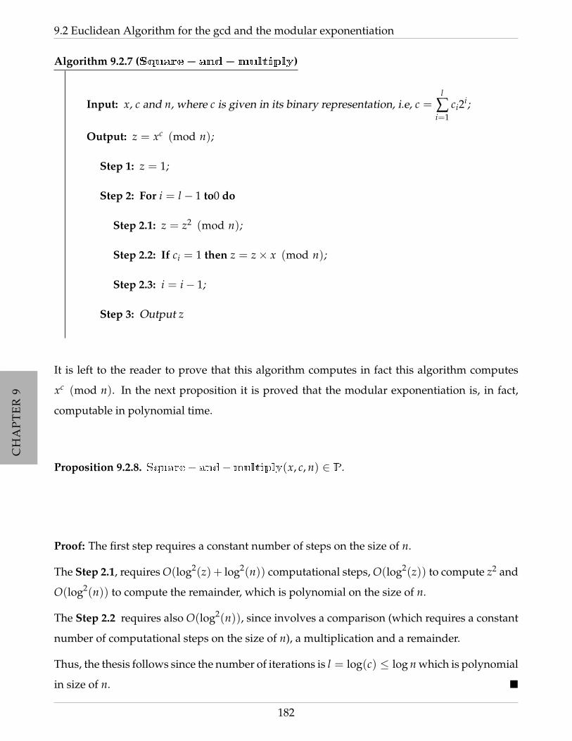
CH

AP

TE

R9

CH

AP

TE

R9

CH

AP

TE

R9

CH

AP

TE

R9

CH

AP

TE

R9

CH

AP

TE

R9

CH

AP

TE

R9

CH

AP

TE

R9


Algorithm 9.2.7 (Square− and−multiply)

Input: x, c and n, where c is given in its binary representation, i.e, c =l

∑i=1

ci2i;

Output: z = xc (mod n);

Step 1: z = 1;

Step 2: For i = l − 1 to0 do

Step 2.1: z = z2 (mod n);

Step 2.2: If ci = 1 then z = z× x (mod n);

Step 2.3: i = i− 1;

Step 3: Output z

It is left to the reader to prove that this algorithm computes in fact this algorithm computes

xc (mod n). In the next proposition it is proved that the modular exponentiation is, in fact,

computable in polynomial time.

Proposition 9.2.8. Square− and−multiply(x, c, n) ∈ P.

Proof: The first step requires a constant number of steps on the size of n.

The Step 2.1, requires O(log2(z) + log2(n)) computational steps, O(log2(z)) to compute z2 and

O(log2(n)) to compute the remainder, which is polynomial on the size of n.

The Step 2.2 requires also O(log2(n)), since involves a comparison (which requires a constant

number of computational steps on the size of n), a multiplication and a remainder.

Thus, the thesis follows since the number of iterations is l = log(c) ≤ log n which is polynomial

in size of n.

182

CH

AP

TE

R9

CH

AP

TE

R9

CH

AP

TE

R9

CH

AP

TE

R9

CH

AP

TE

R9

CH

AP

TE

R9

CH

AP

TE

R9

CH

AP

TE

R9


• • • • • • • • • • • • • • • • • • • • • • • • • • • • • • • • • • • • •

SECTION 9.3

Checking fast primality of numbers

The primality test, i.e., checking if a given number is prime or not is also a crucial for the

RSA process since this cryptographic system relies on the fact that one can produce relatively

fast prime numbers to perform the operations to set the public and the private keys. In the

previous section it was proved that if one have access to prime numbers easily then the RSA

cryptographic system works perfectly under the assumption that one-way functions with trap-

doors exist, more concretely that multiplication of two primes p and q is a one-way function

with trapdoor with p and q.

In 2002, Agrawal, Kayal and Saxena proved that the problem Primes, i.e., checking is a given

number is prime, it is a problem that can be solved with a deterministic polynomial-time

algorithm, by proving that Primes ∈ P. This problem was opened for long time and this

result was a major breakthrough in the last years in computational complexity field. The AKS

algorithm will be discussed in detail in one of the subsequent subsection. One of the issues

concerning this major breakthrough is the practical implementation of the algorithm for testing

primality, since the degree of the polynomial involved in the proof is high and then, although

polynomial, it might require times of computation that seem unfeasible in practice. Contrarily

to this deterministic algorithm and until the appearance of AKS, primality was tested with

randomized polynomial-time algorithms that are allowed to error with a small probability

claiming that a given number is prime when, in fact, it is not. An example of this algorithm is

the so called Solovay–Strassen algorithm that can test primality of a number in quadratic time

on the length of its binary representation.

To motivate the presentation of the probabilistic test of primality to generate parameter for the

RSA cryptographic system consider the following argument. In Theorem 2.2.5 on Page 18, one

already proved that the number of primes less or equal to n is near n/ ln n, and thus, if one

randomly choses a number between 1 and n, then the probability that it is prime is roughly

1/ ln n and thus, on average picking ln n random numbers, one of them is prime. Just for sake

183

CH

AP

TE

R9

CH

AP

TE

R9

CH

AP

TE

R9

CH

AP

TE

R9

CH

AP

TE

R9

CH

AP

TE

R9

CH

AP

TE

R9

CH

AP

TE

R9

9.3 Checking fast primality of numbers

of presentation and understanding consider a more concrete example: pick a number n that

is chosen to be a 1024 bit number which is a multiplication of two primes p and q. Then one

can chose its prime factors with 512 bits. Among the numbers with 512 bits, the probability

of choosing a prime number is approximately 1/ ln 2512 ≈ 1/355 and thus, on average, given

choosing 355 random 512 bit integers one of them will be prime. This argument support the

idea that one can generate sufficiently large random numbers that are almost for sure prime,

and hence parameter generation for the RSA cryptographic system is doable in practice.

In the following it is presented and discussed this two processes for the primality testing but a

few definitions are needed for the sequel, namely the concept of a probabilistic or randomized

algorithm. Like the name suggests, randomized algorithms are algorithms that have access to

some random numbers while a deterministic one does not have access to randomness. This

kind of algorithms define other computational complexity classes other than P or NP. They

are called randomized classes and include RP, co−RP, ZP = RP ∩ (co−RP) and BBP. In

the first case, when a decision problem A is given, the algorithm is always correct on instances

x if x /∈ A and is allowed to error with probability at most 1/2 on instances x ∈ A, the second

one is similar to the first one but with roles inverted concerning the instances, and the latter

one, the algorithm is allowed to give wrong answers on both times of instances. The belonging

relationships among these classes and P and NP are unestablished and are also major open

questions in complexity.

184

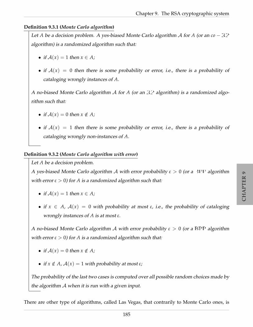
CH

AP

TE

R9

CH

AP

TE

R9

CH

AP

TE

R9

CH

AP

TE

R9

CH

AP

TE

R9

CH

AP

TE

R9

CH

AP

TE

R9

CH

AP

TE

R9


Definition 9.3.1 (Monte Carlo algorithm)

Let A be a decision problem. A yes-biased Monte Carlo algorithm A for A (or an co−RP

algorithm) is a randomized algorithm such that:

• if A(x) = 1 then x ∈ A;

• if A(x) = 0 then there is some probability or error, i.e., there is a probability of

cataloging wrongly instances of A.

A no-biased Monte Carlo algorithm A for A (or an RP algorithm) is a randomized algo-

rithm such that:

• if A(x) = 0 then x /∈ A;

• if A(x) = 1 then there is some probability or error, i.e., there is a probability of

cataloging wrongly non-instances of A.

Definition 9.3.2 (Monte Carlo algorithm with error)

Let A be a decision problem.

A yes-biased Monte Carlo algorithm A with error probability ε > 0 (or a BPP algorithm

with error ε > 0) for A is a randomized algorithm such that:

• if A(x) = 1 then x ∈ A;

• if x ∈ A, A(x) = 0 with probability at most ε, i.e., the probability of cataloging

wrongly instances of A is at most ε.

A no-biased Monte Carlo algorithm A with error probability ε > 0 (or a BPP algorithm

with error ε > 0) for A is a randomized algorithm such that:

• if A(x) = 0 then x /∈ A;

• if x /∈ A, A(x) = 1 with probability at most ε;

The probability of the last two cases is computed over all possible random choices made by

the algorithm A when it is run with a given input.

There are other type of algorithms, called Las Vegas, that contrarily to Monte Carlo ones, is

185

CH

AP

TE

R9

CH

AP

TE

R9

CH

AP

TE

R9

CH

AP

TE

R9

CH

AP

TE

R9

CH

AP

TE

R9

CH

AP

TE

R9

CH

AP

TE

R9


allowed to not give an answer but one it does, it is always correct. In this section the focus is

to know whether or not a given number is prime or composite. The Monte Carlo algorithm

are named this way because to the grand casino in the Principality of Monaco at Monte Carlo,

which is well-known around the world as an icon of gambling. In the following it is formally

describe the problems:

Problem 9.3.1 (Composite)

Instance An integer n ≥ 2;

Question Is n composite?

Problem 9.3.2 (Primes)

Instance An integer n ≥ 2;

Question Is n prime?

Notice that these two problems are complementary, i.e., if n /∈ Composite then n ∈ Primes.

Recall that a decision algorithm is only required to answer 1 or 0 and thus, for example in the

case of Composite it will not give a factorization in case n is composite, which is a search

problem.

The Solovay–Strassen algorithm, is a yes-biased Monte Carlo algorithm for Composite with

error probability 1/2, which means that if the algorithm answers 1 then n is composite for sure

while if n is composite, then the algorithm answers 1 with probability at least 1/2.

Before the formal presentation of the Solovay–Strassen algorithm for primality testing it is

necessary some more background on number theory, namely Legengre’s and Jacobi’s symbol,

that is presented in the next subsection.

186

CH

AP

TE

R9

CH

AP

TE

R9

CH

AP

TE

R9

CH

AP

TE

R9

CH

AP

TE

R9

CH

AP

TE

R9

CH

AP

TE

R9

CH

AP

TE

R9


• • •

9.3.1 The quadratic residue problem and the Legendre

and Jacobi symbols

The quadratic residues is a very important problem in Cryptography that is believed unfeasible

in general but easy to determine for the case where the modulo is taken over a prime or a prime

power. The difficulty arises when the factorization of the modulo is unknown.

Definition 9.3.3 (Quadratic residue modulo p)

Let p be an odd prime and let a be an integer.

One says that a is a quadratic residue modulo p, if a 6≡ 0 (mod p) and the congruence

y2 ≡ a (mod p) has a solution y ∈ Zp.

One says that a is a quadratic non-residue modulo p, if a 6≡ 0 (mod p) and it is not a

quadratic residue modulo p, i.e, the congruence y2 ≡ a (mod p) has no solutions in Zp.

Notice that if p is an odd prime and a is such that y2 ≡ a (mod p), i.e., a is a quadratic residue

modulo p, then also (−y)2 ≡ a (mod p). Since p is odd y 6≡ −y (mod p) and thus the

quadratic congruence x2 ≡ a (mod p) is equivalent to the congruence (x − y)(x + y) ≡ 0

(mod p). Thus, p|(x − y)(x + y) which implies, since p is prime, that p|(x − y) or p|(x + y),

i.e., x = ±y (mod p).

So, this arguments leads to the conclusion that the congruence x2 ≡ a (mod p) has exactly two

solutions (modulo p) that are, in particular, negatives of each other modulo p.

One can now define the Quadratic Residues problem.

Problem 9.3.3 (Quadratic Residuesmodulo primes)

Instance An odd prime p and an integer a ∈ Zp;

Question Is a a quadratic residue modulo p?

The following Euler’s theorem justifies the fact thatQuadratic Residuesmodulo prime num-

bers can be solved in polynomial time.

187

CH

AP

TE

R9

CH

AP

TE

R9

CH

AP

TE

R9

CH

AP

TE

R9

CH

AP

TE

R9

CH

AP

TE

R9

CH

AP

TE

R9

CH

AP

TE

R9


Theorem 9.3.1 (Euler’s Criterion of residues)

Let p be an odd prime and a and integer. The integer a is a quadratic residue modulo p if

and only if

a(p−1)/2 ≡ 1 (mod p)

Proof:

(⇐)

Assume that a is a quadratic residue modulo p, i.e., a 6≡ 0 (mod p) and there is y ∈ Zp such

that y2 ≡ a (mod p). By Fermat’s little theorem 2.3.5 on Page 22, yp−1 ≡ 1 (mod p). Thus:

a(p−1)/2 ≡ (y2)(p−1)/2 (mod p)

≡ y(p−1) (mod p)

≡ 1 (mod p)

(⇒)

Assume that a(p−1)/2 ≡ 1 (mod p) and let b be a generator of Z∗p. Then, by definition of

generator, there exists i ≤ p− 1 such that a ≡ bi (mod p). Then:

(bi)(p−1)/2 ≡ a(p−1)/2 (mod p)

≡ 1 (mod p)

since b is a generator of Z∗p then ord(b) = p − 1 and since (bi)(p−1)/2 ≡ 1 (mod p) then by

Lagrange’s theorem 2.1.1 on Page 11, p− 1∣∣∣∣ i(p− 1)

2, which implies that i/2 is an integer and

hence is even, i.e, there exists k ∈ N such that i = 2k. thus, a ≡ bi (mod p) ≡ (bk)2 (mod p),

and so a is a quadratic residue modulo p.

Notice that by the fact that the Algorithm 9.2.7 of Square− and−multiply runs in poly-

nomial time (proved in Proposition 9.2.8), determining if a(p−1)/2 ≡ 1 (mod p) can be done

in O(log3 p) and thus, the problem Quadratic Residues modulo primes is computable in

polynomial time.

188

CH

AP

TE

R9

CH

AP

TE

R9

CH

AP

TE

R9

CH

AP

TE

R9

CH

AP

TE

R9

CH

AP

TE

R9

CH

AP

TE

R9

CH

AP

TE

R9


Definition 9.3.4 (Legendre symbol)

Let p be an odd prime and let a be an integer. The Legendre symbol is a function Z →

−1, 0, 1, denoted by(

ap

)that is defined as follows:

(ap

)=

0 if a ≡ 0 (mod p)

1 if a is a quadratic residue modulo p

−1 if a is a quadratic non-residue modulo p

In the next example it is realized the connection between Euler’s criterion and the Legendre

symbol for prime numbers.

Example 9.3.4. From Euler’s criterion for residues presented in Theorem 9.3.1 it is clear that(

ap

)= 1

if and only if a(p−1)/2 ≡ 1 (mod p). Also, if a is multiple of p then(

ap

)= 0 and on the other cases(

ap

)= −1.

A more practical example is given now.

Example 9.3.5. (27

)= 1

since 42 ≡ 2 (mod 7).

(57

)= −1

as the reader can easily check, there is not n < 7 such that n2 ≡ 5 (mod 7).

From the example above and again, by Theorem ?? it is easy to derive the following result:

Theorem 9.3.2

Let p be an odd prime and let a be an integer. Then the Legendre symbol can be computed

by:

(ap

)≡ a(p−1)/2 (mod p)

189

CH

AP

TE

R9

CH

AP

TE

R9

CH

AP

TE

R9

CH

AP

TE

R9

CH

AP

TE

R9

CH

AP

TE

R9

CH

AP

TE

R9

CH

AP

TE

R9


It is possible to generalize the Legendre symbol for odd numbers that are not primes. This

generalization is called the Jacobi symbol and is presented in the next definition.

Definition 9.3.5 (Jacobi symbol)

Let n be an odd number and let a be an integer. Assume that the decomposition in prime

factor of n is:

n =k

∏i1

plii .

The Jacobi symbol is a function Z → −1, 0, 1, denoted also by( a

n)

that is defined as

follows:

( an

)=

k

∏i=1

(api

)li.

To prove that the Solovay–Strassen is computable in polynomial-time it will be necessary to

compute the Jacobi symbol. It is not necessary to factor n to compute the Jacobi symbol since

one can use some results from number theory presented below:

Theorem 9.3.3 (Congruent Integers)

Let n be an odd number and let a and b two integers such that a ≡ b (mod n). Then:

( an

)=

(bn

).

Proof: Notice that if a ≡ b (mod p) then the congruence x2 ≡ a (mod p) has a solution if and

only if x2 ≡ b (mod p). So congruent integers are of the same quadratic character and thus

has the same Jacobi symbol.

190

CH

AP

TE

R9

CH

AP

TE

R9

CH

AP

TE

R9

CH

AP

TE

R9

CH

AP

TE

R9

CH

AP

TE

R9

CH

AP

TE

R9

CH

AP

TE

R9


Theorem 9.3.4

Let n be an odd number. Then:

(2n

)=

1 if n ≡ ±1 (mod 8)

−1 if n ≡ ±3 (mod 8)

.

Proof: The statement of the Theorem, by the Euler’s Criterion (Theorem 9.3.1), is equivalent to

prove that:

2(n−1)/2 = (−1)(n2−1)/8 ≡ ±1 (mod n)

depending on the case if n ≡ ±1 (mod 8) or n ≡ ±3 (mod 8). 1

Now the thesis of the result follows from the fact that if n ≡ ±1 (mod 8) then (n2 − 1)/8 is

even and if n ≡ ±3 (mod 8) then (n2 − 1)/8 is odd.

In fact, assume for now that n ≡ 1 (mod 8). Then there exists k such that 8k− 1 = n and thus

n2 = 64k2 − 16k + 1.

So, one has

n2 − 18

= 8k2 − 2k

i.e.,n2 − 1

8is a even number.

The other 3 cases for possible values of n are very similar to this one and are left as exercises

for the interested reader.

1The proof of the equivalence uses a result due to Gauss that it is omitted. A complete proof of this equivalence

can be found in any classical book of number theory.

191

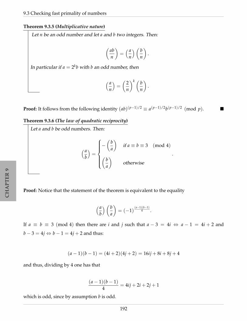
CH

AP

TE

R9

CH

AP

TE

R9

CH

AP

TE

R9

CH

AP

TE

R9

CH

AP

TE

R9

CH

AP

TE

R9

CH

AP

TE

R9

CH

AP

TE

R9


Theorem 9.3.5 (Multiplicative nature)

Let n be an odd number and let a and b two integers. Then:

(abn

)=( a

n

)( bn

).

In particular if a = 2kb with b an odd number, then

( an

)=

(2n

)k ( bn

).

Proof: It follows from the following identity (ab)(p−1)/2 ≡ a(p−1)/2b(p−1)/2 (mod p).

Theorem 9.3.6 (The law of quadratic reciprocity)

Let a and b be odd numbers. Then:

( ab

)=

−(

ba

)if a ≡ b ≡ 3 (mod 4)

(ba

)otherwise

.

Proof: Notice that the statement of the theorem is equivalent to the equality

( ab

)(ba

)= (−1)

(a−1)(b−1)4 .

If a ≡ b ≡ 3 (mod 4) then there are i and j such that a − 3 = 4i ⇔ a − 1 = 4i + 2 and

b− 3 = 4j⇔ b− 1 = 4j + 2 and thus:

(a− 1)(b− 1) = (4i + 2)(4j + 2) = 16ij + 8i + 8j + 4

and thus, dividing by 4 one has that

(a− 1)(b− 1)4

= 4ij + 2i + 2j + 1

which is odd, since by assumption b is odd.

192

CH

AP

TE

R9

CH

AP

TE

R9

CH

AP

TE

R9

CH

AP

TE

R9

CH

AP

TE

R9

CH

AP

TE

R9

CH

AP

TE

R9

CH

AP

TE

R9


On the other hand, assume without loss of generality that a ≡ 1 (mod 4). In this case, a− 1 =

4i for some i and thus (a− 1)(b− 1) = 4i(b− 1) and thus

(a− 1)(b− 1)4

= i(b− 1)

which is even.

Corollary 9.3.6. Let n be an odd number and let a and b two integers. Then:

( nab

)=(n

a

) (nb

).

Next some examples are presented for sake of understanding.

Example 9.3.7. First of all notice that contrarily to the Legendre symbol, if for some a and n,( a

n)= 1,

when n is not prime does not necessarily mean that a is a quadratic residue modulo n. In fact, for

example,

(29

)=

(23

)(23

)= 1

but, as the reader can easily check, modulo 9, 2 is not a quadratic residue.

Example 9.3.8. (12345

331

)=

(3

331

)(5

331

)(823331

)=

(3

331

)(5

331

)(161331

)=

(3

331

)(5

331

)(7

331

)(23331

)= (−1)

(3313

)(331

5

)(−1)

(3317

)(−1)

(33123

)

= −(

13

)(15

)(27

)(3

23

)2

= −(1)(1)(1)(1) = 1

193

CH

AP

TE

R9

CH

AP

TE

R9

CH

AP

TE

R9

CH

AP

TE

R9

CH

AP

TE

R9

CH

AP

TE

R9

CH

AP

TE

R9

CH

AP

TE

R9


• • •

9.3.2 Solovay–Strassen algorithm

Now it is presented the Solovay–Strassen algorithm. It is a yes-biased Monte-Carlo algorithm

for theCompositewith error probability at most 1/2. This test is based on the Euler’s criterion

9.3.1 and works by selecting at random an integer and computing the powers (n− 1)/2 in Zn.

In addition, it computes the Jacobi symbol for these numbers and if the results of both two

calculations are different, then the number is composite.

Since this is a Monte-Carlo algorithm with probability of error 1/2 it is not necessary for the two

calculations to agree when n is composite. In fact, among those numbers which are relatively

prime to n in the set 1, 2, · · · , n− 1 , at most 50% of them get a wrong answer. For any given

integer n, if one wants to decresae the probability of error one can repeat it by picking k integers

uniformly at random and run the basic algorithm. With this repetation one can decrease the

probability to 1/2k which is negligible (when compared with k and n) for sufficiently large k.

Algorithm 9.3.9 (Solovay - Strassen – SS)

Input: An integer n.

Output: 1 if n is prime and 0 otherwise

Step 1: Choose at random a number a between 1 and n− 1;

Step 2: x =( a

n

);

Step 3: If x = 0 then output 0 else

Step 3.1: Use the AlgorithmSquare− and−multiply define of Page 182 to com-

pute the value y = a(n−1)/2 (mod n);

Step 3.2: If x ≡ y (mod n) then output 1 else output 0;

One can call a given composed number n a pseudo-prime if the Solovay–Strassen algorithm

194

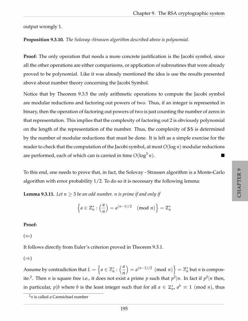
CH

AP

TE

R9

CH

AP

TE

R9

CH

AP

TE

R9

CH

AP

TE

R9

CH

AP

TE

R9

CH

AP

TE

R9

CH

AP

TE

R9

CH

AP

TE

R9


output wrongly 1.

Proposition 9.3.10. The Solovay–Strassen algorithm described above is polynomial.

Proof: The only operation that needs a more concrete justification is the Jacobi symbol, since

all the other operations are either comparisons, or application of subroutines that were already

proved to be polynomial. Like it was already mentioned the idea is use the results presented

above about number theory concerning the Jacobi Symbol.

Notice that by Theorem 9.3.5 the only arithmetic operations to compute the Jacobi symbol

are modular reductions and factoring out powers of two. Thus, if an integer is represented in

binary, then the operation of factoring out powers of two is just counting the number of zeros in

that representation. This implies that the complexity of factoring out 2 is obviously polynomial

on the length of the representation of the number. Thus, the complexity of SS is determined

by the number of modular reductions that must be done. It is left as a simple exercise for the

reader to check that the computation of the Jacobi symbol, at most O(log n) modular reductions

are performed, each of which can is carried in time O(log3 n).

To this end, one needs to prove that, in fact, the Solovay - Strassen algorithm is a Monte-Carlo

algorithm with error probability 1/2. To do so it is necessary the following lemma:

Lemma 9.3.11. Let n ≥ 3 be an odd number. n is prime if and only ifa ∈ Z∗n :

( an

)= a(n−1)/2 (mod n)

= Z∗n

Proof:

(⇐)

It follows directly from Euler’s criterion proved in Theorem 9.3.1.

(⇒)

Assume by contradiction that L =

a ∈ Z∗n :( a

n

)= a(n−1)/2 (mod n)

= Z∗n but n is compos-

ite.2. Then n is square free i.e., it does not exist a prime p such that p2|n. In fact if p2|n then,

in particular, p|b where b is the least integer such that for all a ∈ Z∗n, ab ≡ 1 (mod n), thus

2n is called a Carmichael number

195

CH

AP

TE

R9

CH

AP

TE

R9

CH

AP

TE

R9

CH

AP

TE

R9

CH

AP

TE

R9

CH

AP

TE

R9

CH

AP

TE

R9

CH

AP

TE

R9


by Fermat’s little theorem 2.3.5, p|n− 1. Since p2|n, p|n and thus p|n− 1− n, i.e., p|1 which

contradicts the fact that p was taken to be a prime number.

Since n is square free n = pr for some prime p and r > 1 such that gcd(p, r) = 1. Let g be a

non-quadratic residue modulo p and consider a ≡ g (mod n) and a ≡ 1 (mod r). Thus by

Theorem 9.3.6 one has: ( an

)=

(ap

)( ar

)=

(gp

)(1r

)= (−1) · 1 = −1

Since( a

n)= a(n−1)/2 (mod n) and since a(p−1)/2 ≡ −1 (mod p) then by the Chinese remain-

der theorem 2.3.4, one concludes that a(p−1)/2 ≡ −1 (mod r) contradiction the fact that a was

chosen such that a ≡ 1 (mod r).

Theorem 9.3.7

If n is an odd prime, and a ∈ 1, · · · , n− 1, then

Pr[SS(a) = 1] = 1.

If n is an odd composite, then

Pr[SS(a) = 0] ≥ 12

.

Proof: If n is an odd prime, then by the previous lemma the Jacobi symbol( a

n

)coincides

always with a(p−1)/2 (mod n) and thus, it is always the case that SS(n) = 1.

Assume know that n is an odd composite number. From the lemma above it follows that

L 6= Z∗n. The reader will have no trouble to show that L is, in fact, a non trivial subgroup of Z∗n.

Thus, by Lagrange theorem 2.1.1 on Page 11, ord(L)|φ(n), hence #L ≤ n− 12

. Thus

Pr[SS(n) = 1] = Pr[gcd(a, n) = 1∧ a ∈ L] =#L

n− 1≤ 1

2

196

CH

AP

TE

R9

CH

AP

TE

R9

CH

AP

TE

R9

CH

AP

TE

R9

CH

AP

TE

R9

CH

AP

TE

R9

CH

AP

TE

R9

CH

AP

TE

R9


• • •

9.3.3 Miller-Rabin’s algorithm for primality test

In this section it is briefly another algorithm that is also a Monte-Carlo algorithm with proba-

bility of error 1/2.

Algorithm 9.3.12 (Miller-Rabin –MR)

Input: An integer n.

Output: 1 if n is prime and 0 otherwise

Step 1: Compute n− 1 = 2sd with d odd.

Step 2: Choose at random a number a between 1 and n− 1;

Step 3: a0 = ad (mod n);

Step 4: If a0 = 1 then output 1 else

Step 4.1: For i = 0 tos do

Step 4.1.1: If a0 = −1 then output 1 else

Step 4.1.1.1: a0 = a20 (mod n)

Step 5 output 0

This algorithm is clearly a polynomial-time algorithm and the details of the proof of that fact

are left for the interested reader.

Notice again that if the answer is that n is compose then certainly n is not prime. But if the

answer is n is prime, then n could still be composite, though the probability that we get the

wrong answer is at most 1/2.

Theorem 9.3.8

If n is a prime number then MR(n) = 1.

197

CH

AP

TE

R9

CH

AP

TE

R9

CH

AP

TE

R9

CH

AP

TE

R9

CH

AP

TE

R9

CH

AP

TE

R9

CH

AP

TE

R9

CH

AP

TE

R9


Proof: Assume that n is prime and MR(n) = 0. Notice that if MR(n) = 0 then it must be the

case that ad ≡ 1 (mod n). Let a be the sequence of values tested in the algorithm. Since ai is

squared in each iteration of the For loop this means that it is tested the values of the form ad,

a2d, · · · , a2s−1d. Hence, it must be case that a2id 6≡ −1 (mod n) for all 0 ≤ i < s− 1.

On the other hand, since n is is prime, by Fermat’s little theorem 2.3.5 one concludes that a2s ≡ 1

(mod n) since n− 1 = 2sd which means that a2s−1d is a square root of 1 modulo n. Since n is

prime, there are only two square roots of 1 modulo n, namely, ±1 (mod n). Since a2k−1d 6≡ −1

(mod n), then a2k−1d ≡ −1 (mod n). By repeating this process with a2k−2d and so on obtains

am ≡ 1 (mod n), which is a contradiction, since the algorithm would have outputted 1 in that

case.

• • •

9.3.4 The AKS algorithm proving that Primes ∈ P

In this section, it is presented the AKS primality test. The name AKS is due to the fact that

it was purposed in 2002 by Agrawal, Kayal and Saxena in [?] and is was one of the major

breakthrough on computational complexity problems with clear applications to cryptography.

Notice that from the fact that one can test is a number is prime or not, does not any anything

about, in the case that a number is not prime, of its prime factors.It is the first provably

deterministic algorithm that one can use to determine whether a given number n is prime or not

within a time which is guaranteed to be polynomial in the number of digits, in fact O(logc n)

for some constant c that will be determine later on in this section. In the previous sections, all

primality testing algorithms were probabilistic but their advantage concerning this algorithm

that is deterministic, is the fact that their running time is much slower, in fact a degree of the

polynomials involved are at most cubic while this one is, a polynomial that for practical reasons

is very high. This question is related with Factoring problem but, for the moment of the writing

of these notes, they are not known to be equivalent from the computational complexity point

of view.

The story of this algorithm starts in 1999 with Agarwal and Biswas when they proposed a

probabilistic algorithm that picking a monic polynomial Q ∈ Zn[x] of degree poly(log n)

uniformly at random and test if (x + a)n ≡ xn + a (mod Q) to derive thew conclusion of

198

CH

AP

TE

R9

CH

AP

TE

R9

CH

AP

TE

R9

CH

AP

TE

R9

CH

AP

TE

R9

CH

AP

TE

R9

CH

AP

TE

R9

CH

AP

TE

R9


primality of n. Since the degree of Q is small then this algorithm is an efficient one and one can

use power method to compute (x + a)n (mod Q) in poly log n time. The correctness follows

from the facts: 1) that with probability at least1

deg Q, Q is irreducible over Zn[x]. Notice that

if d = deg Q, then xqd − x = ∏p

p where in the product are considered all polynomials p that

irreducible and have degree which divides d and since there are at least qd

d irreducible polyno-

mials of degree dividing d, and since there are a total of qd choices for monic polynomials of Q

over Zp[x], at least with probability 1d we will get a polynomial Q that is irreducible over Zp[x],

and then of course Q is also irreducible module n. Also the probability that (x + a)n ≡ xn + a

(mod Q) if n is composite is very very small due to the Chinese Reminder Theorem. In fact, if

(x+ a)n ≡ xn + a (mod Q)) holds for many polynomials Q1, Q2, . . . , Qt’s, then the congruence

also holds module with the least common multiplier due to Chinese Reminder Theorem, but

when the degree of that polynomial exceeds n one has (x + a)n ≡ xn + a (mod n) as well

because the degree on both sides are only n, contradicting the fact that n is composite.

So the basic idea of AKS algorithm is to explore polynomial identities. In fact, it relies on

polynomial identities that are known to be true modulo prime numbers and cannot hold

for non-prime numbers since if they were true than a large number of additional polyno-

mial identities could be generated, eventually violating the factor theorem that asserts that

a polynomial identity of degree at most d can be obeyed by at most d values of the unknown

variable. Consider again the Fermat’s little theorem presented in Theorem 2.3.5 on page 22

that states that for any prime number p, ap ≡ a (mod p). On may think that this theorem

can be used to primality test with the following argument: to test whether a number n is

prime, pick a few values of a and see whether an ≡ a (mod n) and determine that n is not

prime if the equality fails for some a. Unfortunately, by the same reason that the Solovay–

Strassen algorithm is Monte-Carlo one, the converse of this argument is also not true, i.e., there

are non-prime numbers, for example, the Carmichael numbers, for which the stated equality

holds for all numbers that are co-prime to n. So Fermat’s little theorem cannot be used, by

itself, to establish primality for general numbers, because it is too weak to eliminate all non-

prime numbers.3 However, there is a stronger version of Fermat’s little theorem which does

eliminate all non-prime numbers and is called polynomial identity that is stated below. The

3The situation improves though for more special types of number. In particular,, for the Mersenne numbers.

199

CH

AP

TE

R9

CH

AP

TE

R9

CH

AP

TE

R9

CH

AP

TE

R9

CH

AP

TE

R9

CH

AP

TE

R9

CH

AP

TE

R9

CH

AP

TE

R9


identity presented obviously implies the Fermat’s little theorem, but the proof also relies on

the Fermat’s little theorem.

Theorem 9.3.9 (polynomial identity)

Let n and a be two numbers.

• If n is prime then (x− a)n ≡ xn − a (mod n).

• If n is composite and gcd(a, n) = 1, then (x− a)n 6≡ xn − a (mod n).

Proof: By Newton’s binomial expansion,

(x− a)n =n

∑i=0

(ni

)xian−i

Thus, if n is prime then(

ni

)then n

∣∣∣∣(ni

)for all 1 < i < n

On the other hand if n is a composite number then there are other terms in the Newton’s

binomial expansion that is not divisible by n. It is left for the interested reader, to give an

example of such a term.

Conversely, if (x − a)n ≡ xn − a (mod n) for some a coprime to n, then by comparing coeffi-

cients using the binomial theorem we see that(

ni

)is divisible by n for all 1 ≤ i ≤ n. But if n is

divisible by some smaller prime p, then by setting i equal to the largest power of p that divides

n, one sees that(

ni

)is not divisible by enough powers of p to be divisible by n, a contradiction.

Thus one can use (x − a)n ≡ xn − a (mod n) (for a single value of a coprime to n) to decide

whether n is prime or not.

So the idea of AKS seems simple. Just by looking at all the elements of the nth row of Pascal’s

triangle one can decide if n is prime or not. At this point the reader should be alerted that this

simple idea does not work efficiently and the reason why is simply: the nth row of Pascal’s

triangle has n + 1 elements which is exponential on the size of n, which is O(log n). So in oder

to design an algorithm that runs in polynomial time for testing primality one needs to “reduce”

all these terms up to just the computation of a polynomial number of them.

200

CH

AP

TE

R9

CH

AP

TE

R9

CH

AP

TE

R9

CH

AP

TE

R9

CH

AP

TE

R9

CH

AP

TE

R9

CH

AP

TE

R9

CH

AP

TE

R9


This can be done by descending to a quotient ring of Zn[x], such as Zn[x]/(xr − 1) for some r.

Clearly, if the identity (x− a)n = xn − a holds in Zn[x], then it will also hold in Zn[x]/(xr − 1),

thus

(x− a)n ≡ xn − a (mod n, xr − 1)

Notice that with this trick, if r is not too large (i.e., it is at most a logarithmic term of n, which

means that the length of r is polynomial on the length of n), the left-hand side of equality

presented above can now be computed efficiently by expanding n in binary and performing

repeated squaring, because all polynomials can be reduced to be of degree less than r, rather

than being as large as n as it will be explained below. Indeed, if r ∈ O(logc n) for some constant

c, then one can induce roots modulo n and thus test the validity of the equality (x − a)n ≡

xn − a (mod xr − 1) in time polynomial time on the size of n as stated in the next theorem:

Theorem 9.3.10

Let n, a and r be non-nulls integers. Assume that for some constant c, for all r ≤ O(logc n),

(x − a)n ≡ xn − a (mod n, xr − 1) holds, and gcd(a, n) = 1. Then n is either a prime

number, or a power of a prime number.

Notice that the computation of gcd(a, n) = 1 can be quickly tested using the Euclides algo-

rithm ??, and if gcd(a, n) 6= 1 then n is of course composite. On the other hand, it is easy to

quickly test for the property that n is a power of an integer. The reader is asked to design an

algorithm to test this property in polynomial time. The idea is to compute the roots n1/k for

1 ≤ k ≤ log2 n, and such powers are clearly composite. Thus, combining this result with the

equality (x − a)n ≡ xn − a (mod n), one can design a deterministic polynomial-time test for

primality.

Theorem 9.3.11 (AKS theorem, key step)

Let n, a and r be non-nulls integers be such that gcd(r, n) = 1 and such that n has order

greater than log2 n in the multiplicative group Z∗r . Assume that for all 1 ≤ r ≤ O(logc n)

for some c, one has (x− a)n ≡ xn − a (mod n, xr − 1), and gcd(a, n) = 1. Then n is either a

prime number, or a power of a prime number.

To find an with the above properties we have

201

CH

AP

TE

R9

CH

AP

TE

R9

CH

AP

TE

R9

CH

AP

TE

R9

CH

AP

TE

R9

CH

AP

TE

R9

CH

AP

TE

R9

CH

AP

TE

R9


Lemma 9.3.13 (Existence of good r). Let n, a and r be non-nulls integers. There exists 1 ≤ r ≤

O(logc n) coprime to n, such that n has order greater than log2 n in the multiplicative group Z∗r .

Proof: For each 1 ≤ k ≤ log2 n, the number ni − 1 has, by the fundamental theorem of

arithmetic, at most O(logc n) for some c prime divisors. If one picks r to be the first prime

not equal to any of these prime divisors, one obtains the claim.

It is clear that Theorem 9.3.10 follows from Theorem 9.3.11 and the Lemma 9.3.13. It is then

sufficient to prove Theorem 9.3.11.

Proof:[of Theorem 9.3.11] If Theorem 9.3.11 fails then it means that n is divisible by some

smaller prime p, but is not a power of p. Since n is coprime to all numbers of size O(logc n) for

all c, i.e. p is not of polylogarithmic size. Moreover, since r is coprime to n, it follows that r is

not a multiple of p.

Let F be a field F = Fp/h(x) where h(x) is a factor in Fp of the rth cyclotomic polynomial

Φr(X) = ∏1≤k≤n−1∧gcd(n,k)=1

(x− e2iπk/n).

From the hypothesis that (x + a)n = xn + a (mod n, xr − 1), one concludes that

(x + a)n = xn + a

in F for all 1 ≤ a ≤ c′r logc n for some c′ and all c′. Notice that n is coprime to every integer

less than c′r logc n, and thus c′r logc n < p.

Also (x + a)p = xp + a also holds in F for all such a. These two equations give

(x + a)n/p = (xp)n/p + a

Notice that the pth power the rth of a primitive root of unity x is again a primitive rth root of

unity 4 and hence we also have

4The converse also holds, in the sense that all primitive rth root is of this form

202

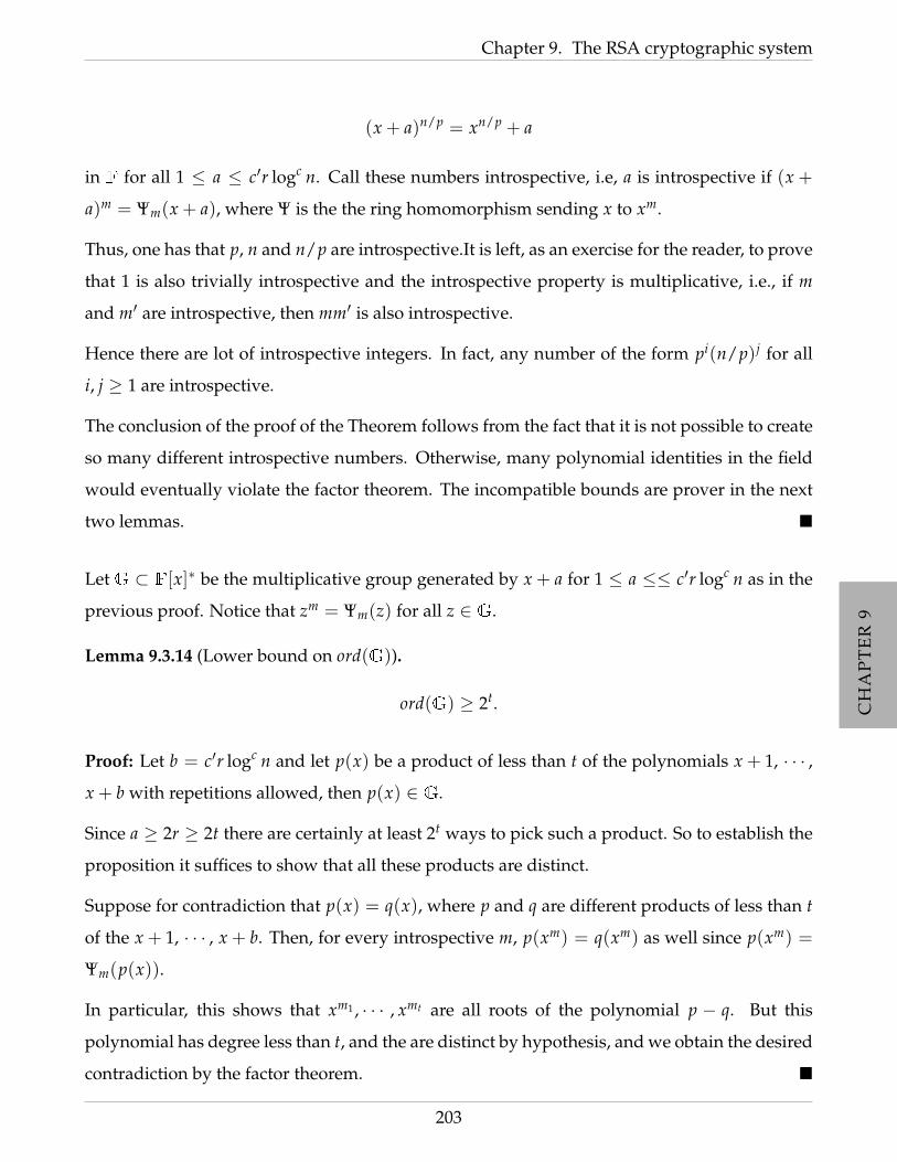
CH

AP

TE

R9

CH

AP

TE

R9

CH

AP

TE

R9

CH

AP

TE

R9

CH

AP

TE

R9

CH

AP

TE

R9

CH

AP

TE

R9

CH

AP

TE

R9


(x + a)n/p = xn/p + a

in F for all 1 ≤ a ≤ c′r logc n. Call these numbers introspective, i.e, a is introspective if (x +

a)m = Ψm(x + a), where Ψ is the the ring homomorphism sending x to xm.

Thus, one has that p, n and n/p are introspective.It is left, as an exercise for the reader, to prove

that 1 is also trivially introspective and the introspective property is multiplicative, i.e., if m

and m′ are introspective, then mm′ is also introspective.

Hence there are lot of introspective integers. In fact, any number of the form pi(n/p)j for all

i, j ≥ 1 are introspective.

The conclusion of the proof of the Theorem follows from the fact that it is not possible to create

so many different introspective numbers. Otherwise, many polynomial identities in the field

would eventually violate the factor theorem. The incompatible bounds are prover in the next

two lemmas.

Let G ⊂ F[x]∗ be the multiplicative group generated by x + a for 1 ≤ a ≤≤ c′r logc n as in the

previous proof. Notice that zm = Ψm(z) for all z ∈ G.

Lemma 9.3.14 (Lower bound on ord(G)).

ord(G) ≥ 2t.

Proof: Let b = c′r logc n and let p(x) be a product of less than t of the polynomials x + 1, · · · ,

x + b with repetitions allowed, then p(x) ∈ G.

Since a ≥ 2r ≥ 2t there are certainly at least 2t ways to pick such a product. So to establish the

proposition it suffices to show that all these products are distinct.

Suppose for contradiction that p(x) = q(x), where p and q are different products of less than t

of the x + 1, · · · , x + b. Then, for every introspective m, p(xm) = q(xm) as well since p(xm) =

Ψm(p(x)).

In particular, this shows that xm1 , · · · , xmt are all roots of the polynomial p − q. But this

polynomial has degree less than t, and the are distinct by hypothesis, and we obtain the desired

contradiction by the factor theorem.

203

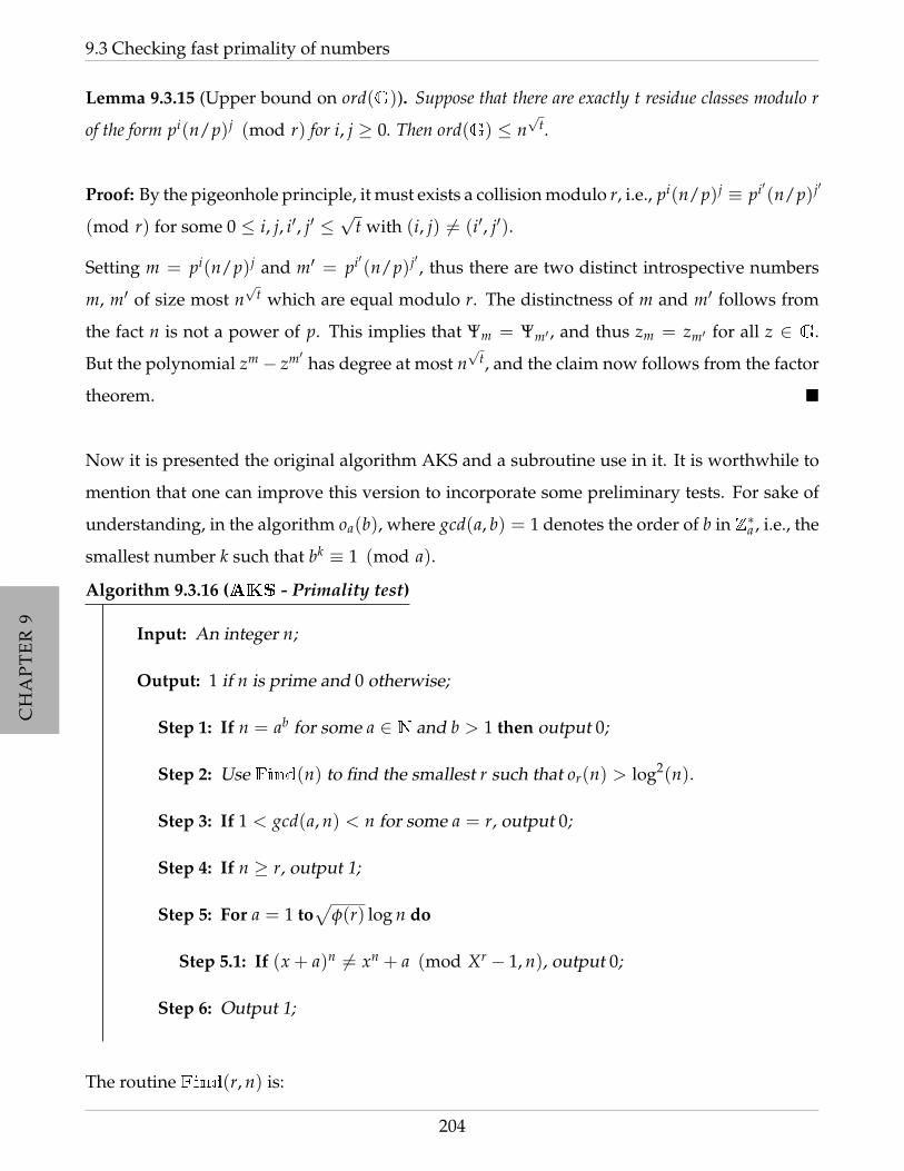
CH

AP

TE

R9

CH

AP

TE

R9

CH

AP

TE

R9

CH

AP

TE

R9

CH

AP

TE

R9

CH

AP

TE

R9

CH

AP

TE

R9

CH

AP

TE

R9


Lemma 9.3.15 (Upper bound on ord(G)). Suppose that there are exactly t residue classes modulo r

of the form pi(n/p)j (mod r) for i, j ≥ 0. Then ord(G) ≤ n√

t.

Proof: By the pigeonhole principle, it must exists a collision modulo r, i.e., pi(n/p)j ≡ pi′(n/p)j′

(mod r) for some 0 ≤ i, j, i′, j′ ≤√

t with (i, j) 6= (i′, j′).

Setting m = pi(n/p)j and m′ = pi′(n/p)j′ , thus there are two distinct introspective numbers

m, m′ of size most n√

t which are equal modulo r. The distinctness of m and m′ follows from

the fact n is not a power of p. This implies that Ψm = Ψm′ , and thus zm = zm′ for all z ∈ G.

But the polynomial zm − zm′ has degree at most n√

t, and the claim now follows from the factor

theorem.

Now it is presented the original algorithm AKS and a subroutine use in it. It is worthwhile to

mention that one can improve this version to incorporate some preliminary tests. For sake of

understanding, in the algorithm oa(b), where gcd(a, b) = 1 denotes the order of b in Z∗a , i.e., the

smallest number k such that bk ≡ 1 (mod a).

Algorithm 9.3.16 (AKS - Primality test)

Input: An integer n;

Output: 1 if n is prime and 0 otherwise;

Step 1: If n = ab for some a ∈ N and b > 1 then output 0;

Step 2: Use Find(n) to find the smallest r such that or(n) > log2(n).

Step 3: If 1 < gcd(a, n) < n for some a = r, output 0;

Step 4: If n ≥ r, output 1;

Step 5: For a = 1 to√

φ(r) log n do

Step 5.1: If (x + a)n 6= xn + a (mod Xr − 1, n), output 0;

Step 6: Output 1;

The routine Find(r, n) is:

204

CH

AP

TE

R9

CH

AP

TE

R9

CH

AP

TE

R9

CH

AP

TE

R9

CH

AP

TE

R9

CH

AP

TE

R9

CH

AP

TE

R9

CH

AP

TE

R9


Algorithm 9.3.17 (Find(n))

Input: An integers n;

Output: 0 if the process fails, or r the smallest one such that or(n) > log2(n);

Step 1: r = 1.

Step 2: While r < n do

Step 2.1: If gcd(r, n) > 1 output 0 else

Step 2.1.1: Set q be the largest prime factor of r;

Step 2.1.2: If a ≥ 4√

r log n and nr−1

q 6≡ 1 mod r, output r;

Step 2.2: r = r + 1.

The complexity of Find(r, n) can be established using the following lemma:

Lemma 9.3.18. Let n be a positive integer. Let r be an appropriated number for the AKS Algorithm on

Step 2. Then r ≤ max3, log5 n such that or(n) > log2 n.

Proof: The cases r = 2 and r = 3 are easy to see that verifies the conditions of the lemma and

are left as exercises for the reader.

Assume that n > 2. Then, dlog5 ne > 10 and thus, if lcm(n) represents the least common

multiplier of all number up to n, then lcm(n) > 2n.5

Notice that the largest value of k such that for any number of the form mk = B = dlog5 ne for

m ≥ 2, is blog Bc. Consider the smallest number r that does not divide

nblog Bc ·blog2 nc

∏i=1

(ni − 1).

gcd(r, n) is not divisible by all the prime divisors of r since otherwise, by the discussion above

r would divide nblog Bc. Therefore, r/gcd(r, n) does not divide the above product. From the

fact that r is the smallest number not dividing the product above, it follows that gcd(r, n) = 1.

5The reader should find no troubles proving this result. In fact, if n > 7, then result holds.

205

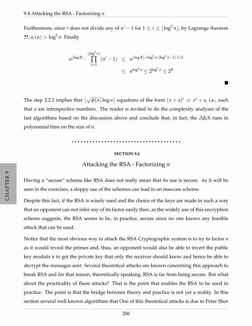
CH

AP

TE

R9

CH

AP

TE

R9

CH

AP

TE

R9

CH

AP

TE

R9

CH

AP

TE

R9

CH

AP

TE

R9

CH

AP

TE

R9

CH

AP

TE

R9

9.4 Attacking the RSA - Factorizing n

Furthermore, since r does not divide any of ni − 1 for 1 ≤ i ≤ blog2 nc, by Lagrange theorem

??, or(n) > log2 n. Finally

nblog Bc ·blog2 nc

∏i=1

(ni − 1) ≤ nblog Bc+log2 n·(log2 n−1)·1/2

≤ nlog4 n ≤ 2log5 n ≤ 2B

The step 2.2.2 implies that b√

φ(n) log nc equations of the form (x + a)r ≡ xr + a, i.e., such

that a are introspective numbers. The reader is invited to do the complexity analyses of the

last algorithms based on the discussion above and conclude that, in fact, the AKS runs in

polynomial time on the size of n.

• • • • • • • • • • • • • • • • • • • • • • • • • • • • • • • • • • • • •

SECTION 9.4

Attacking the RSA - Factorizing n

Having a “secure” scheme like RSA does not really mean that its use is secure. As it will be

seen in the exercises, a sloppy use of the schemes can lead to an insecure scheme.

Despite this fact, if the RSA is wisely used and the choice of the keys are made in such a way

that an opponent can not infer any of its factor easily then, as the widely use of this encryption

scheme suggests, the RSA seems to be, in practice, secure since no one knows any feasible

attack that can be used.

Notice that the most obvious way to attack the RSA Cryptographic system is to try to factor n

as it would reveal the primes and, thus, an opponent would also be able to invert the public

key modulo n to get the private key that only the receiver should know and hence be able to

decrypt the messages sent. Several theoretical attacks are known concerning this approach to

break RSA and for that reason, theoretically speaking, RSA is far from being secure. But what

about the practicality of these attacks? That is the point that enables the RSA to be used in

practice. The point is that the bridge between theory and practice is not yet a reality. In this

section several well known algorithms that One of this theoretical attacks is due to Peter Shor

206

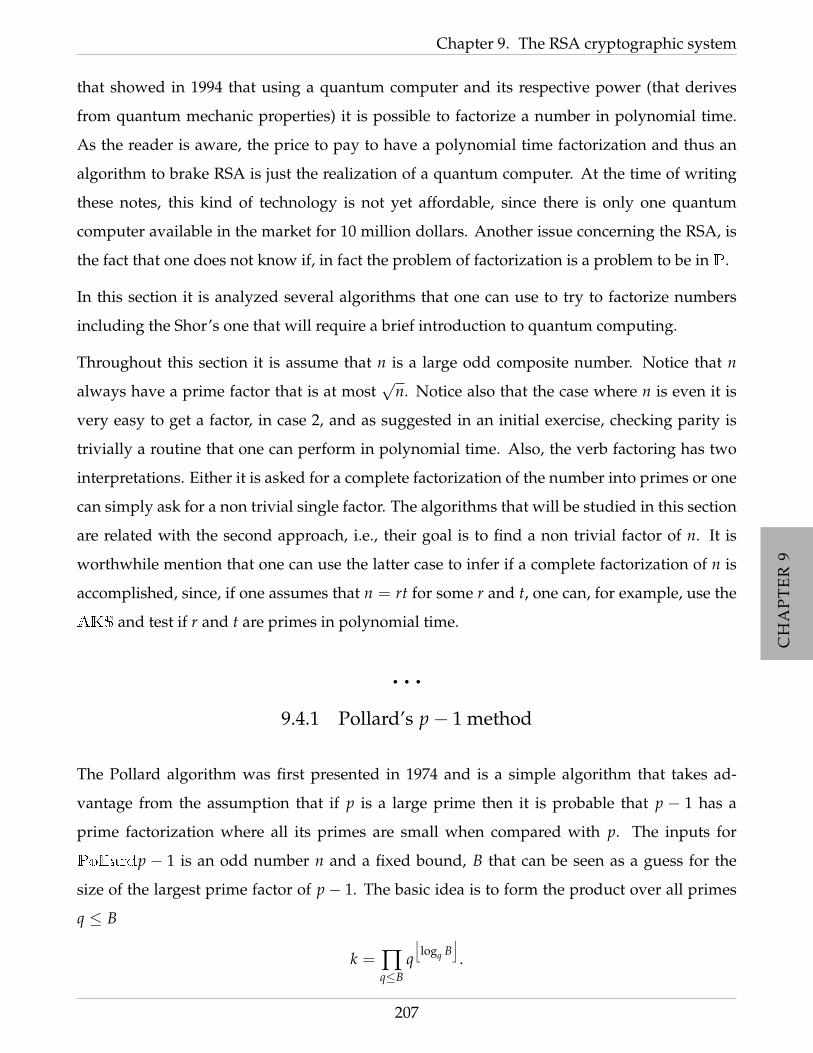
CH

AP

TE

R9

CH

AP

TE

R9

CH

AP

TE

R9

CH

AP

TE

R9

CH

AP

TE

R9

CH

AP

TE

R9

CH

AP

TE

R9

CH

AP

TE

R9


that showed in 1994 that using a quantum computer and its respective power (that derives

from quantum mechanic properties) it is possible to factorize a number in polynomial time.

As the reader is aware, the price to pay to have a polynomial time factorization and thus an

algorithm to brake RSA is just the realization of a quantum computer. At the time of writing

these notes, this kind of technology is not yet affordable, since there is only one quantum

computer available in the market for 10 million dollars. Another issue concerning the RSA, is

the fact that one does not know if, in fact the problem of factorization is a problem to be in P.

In this section it is analyzed several algorithms that one can use to try to factorize numbers

including the Shor’s one that will require a brief introduction to quantum computing.

Throughout this section it is assume that n is a large odd composite number. Notice that n

always have a prime factor that is at most√

n. Notice also that the case where n is even it is

very easy to get a factor, in case 2, and as suggested in an initial exercise, checking parity is

trivially a routine that one can perform in polynomial time. Also, the verb factoring has two

interpretations. Either it is asked for a complete factorization of the number into primes or one

can simply ask for a non trivial single factor. The algorithms that will be studied in this section

are related with the second approach, i.e., their goal is to find a non trivial factor of n. It is

worthwhile mention that one can use the latter case to infer if a complete factorization of n is

accomplished, since, if one assumes that n = rt for some r and t, one can, for example, use the

AKS and test if r and t are primes in polynomial time.

• • •

9.4.1 Pollard’s p− 1 method

The Pollard algorithm was first presented in 1974 and is a simple algorithm that takes ad-

vantage from the assumption that if p is a large prime then it is probable that p − 1 has a

prime factorization where all its primes are small when compared with p. The inputs for

Pollardp − 1 is an odd number n and a fixed bound, B that can be seen as a guess for the

size of the largest prime factor of p− 1. The basic idea is to form the product over all primes

q ≤ B

k = ∏q≤B

q⌊

logq B⌋.

207

CH

AP

TE

R9

CH

AP

TE

R9

CH

AP

TE

R9

CH

AP

TE

R9

CH

AP

TE

R9

CH

AP

TE

R9

CH

AP

TE

R9

CH

AP

TE

R9


Thus, it is expectable that k is highly divisible by all the small primes that one also expects

to divide p − 1, and hence one expects that p − 1 to divide k. So, by Fermat’s little theorem

presented on page 22 it is known that p|ak − 1 for all a ∈ Zp − 0 and hence clearly p|d where

d is the greatest common divisor of ak − 1 and n and so using the Euclides algorithm one can

find efficiently on the size of n a nontrivial factor d of n.

Algorithm 9.4.1

Input: n and a bound B;

Output: either a non trivial factor of n or failure;

Step 1: a = 2;

Step 2: For j = 2 to B do

Step 2.1: a = aj (mod n);

Step 3: d = Euclides(a− 1, n);

Step 4: If 1 < d < n then output d else output failure;

This algorithm, runs in O(B log B(log2 n) + log3 n) steps, since it requires only B− 1 modular

exponentiations each costing at most 2 log2 B steps by using theSQUARE−AND−MULTIPLY

algorithm presented in Page 182, and the computation of the gcd can be performed in time

O(log3 n). Thus if B is of order logc n for some integer c, then the algorithm is indeed a

polynomial-time algorithm as a function of the size of n. The drawback of this algorithm is

that with such a choice of B, the probability of success will be very small. On the other hand,

if the size of B is near√

n, then the algorithm is guaranteed to be successful, but it will be no

faster than trial division.

In the next example it is presented an use of the Polaroid method for factoring an integer n.

Example 9.4.2. Let n be the number 6380651 and choose B = 9. Thus:

k = 23 · 32 · 5 · 7 = 2520 = 212 + 28 + 27 + 26 + 24 + 23.

208

CH

AP

TE

R9

CH

AP

TE

R9

CH

AP

TE

R9

CH

AP

TE

R9

CH

AP

TE

R9

CH

AP

TE

R9

CH

AP

TE

R9

CH

AP

TE

R9


The computation of k can be easily done by repeated squaring modulo 6380651

21 = 2 22 = 4 24 = 16 28 = 256

216 = 65536 232 = 789173 264 = 4202423 2128 = 5994431

2256 = 5409973 2512 = 4188467 21024 = 440743 22048 = 1853005,

so

2k − 1 ≡ 256 · 65536 · 420243 · 5994431 · 5409973 · 1853005− 1 ≡ 6347878 (mod 6380651).

Using Euclides algorithm to determine the gcd(6380651, 6347878) one gets as output 2521, since

6380651 = 6347878 + 32773

6347879 = 193 · 32773 + 22689

32773 = 22689 + 10084

22689 = 2 · 10084 + 2521

10084 = 4 · 2521 + 0,

So 2521|6380651, giving the factorization of n as:

6380651 = 2521 · 2531.

There exists a derivation of this method called Pollard Rho method that takes advantage of

some other properties of divisors of numbers to zoom in on a factor quite quickly. It is sug-

gested to the reader the reading of [Sti06] for details on this method of factorization.

• • •

9.4.2 Dixon’s random square algorithms

Dixon’s algorithm is an improvement over Fermat’s factorization method6 that tries to find x

and y efficiently by computing x, y ∈ Zn such that x2 ≡ y2 (mod n). Then with probability ≥6Fermat’s factorization method is basically a method to find integers x and y such that n = x2 − y2 = (x +

y)(x− y) and uses that fact to factor n.

209

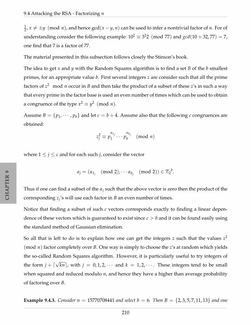
CH

AP

TE

R9

CH

AP

TE

R9

CH

AP

TE

R9

CH

AP

TE

R9

CH

AP

TE

R9

CH

AP

TE

R9

CH

AP

TE

R9

CH

AP

TE

R9


12 , x 6= ±y (mod n), and hence gcd(x− y, n) can be used to infer a nontrivial factor of n. For of

understanding consider the following example: 102 ≡ 322 (mod 77) and gcd(10 + 32, 77) = 7,

one find that 7 is a factor of 77.

The material presented in this subsection follows closely the Stinson’s book.

The idea to get x and y with the Random Squares algorithm is to find a set B of the b smallest

primes, for an appropriate value b. First several integers z are consider such that all the prime

factors of z2 mod n occur in B and then take the product of a subset of these z’s in such a way

that every prime in the factor base is used an even number of times which can be used to obtain

a congruence of the type x2 ≡ y2 (mod n).

Assume B = p1, · · · , pb and let c = b + 4. Assume also that the following c congruences are

obtained:

z2j ≡ p

α1j1 · · · p

αbjb (mod n)

where 1 ≤ j ≤ c and for each such j, consider the vector

aj = (α1j (mod 2), · · · αbj (mod 2)) ∈ Z2b.

Thus if one can find a subset of the αj such that the above vector is zero then the product of the

corresponding zj’s will use each factor in B an even number of times.

Notice that finding a subset of such c vectors corresponds exactly to finding a linear depen-

dence of these vectors which is guaranteed to exist since c > b and it can be found easily using

the standard method of Gaussian elimination.

So all that is left to do is to explain how one can get the integers z such that the values z2

(mod n) factor completely over B. One way is simply to choose the z’s at random which yields

the so-called Random Squares algorithm. However, it is particularly useful to try integers of

the form j + d√

kne, with j = 0, 1, 2, · · · and k = 1, 2, · · · . These integers tend to be small

when squared and reduced modulo n, and hence they have a higher than average probability

of factoring over B.

Example 9.4.3. Consider n = 15770708441 and select b = 6. Then B = 2, 3, 5, 7, 11, 13 and one

210

CH

AP

TE

R9

CH

AP

TE

R9

CH

AP

TE

R9

CH

AP

TE

R9

CH

AP

TE

R9

CH

AP

TE

R9

CH

AP

TE

R9

CH

AP

TE

R9


has the following three congruences:

83409341562 ≡ 3 · 7 (mod n)

120449429442 ≡ 2 · 7 · 13 (mod n)

27737000112 ≡ 2 · 3 · 13 (mod n)

Then, the product of these three congruences, one also has

(8340934156 · 12044942944 · 2773700011)2 ≡ (2 · 3 · 7 · 13)2 (mod n).⇔

95034357852 ≡ 5462 (mod n)

So EUCLIDES(9503435785− 546, 15770708441) = 115759, and thus 115759|15770708441.

Now one can consider the following vectors:

a1 = (0, 1, 0, 1, 0, 0)

a2 = (1, 0, 0, 1, 0, 1)

a3 = (1, 1, 0, 0, 0, 1)

It follows that

a1 + a2 + a3 = (0, 0, 0, 0, 0, 0) (mod 2).

This gives rise to the congruence above that successfully allows a factorization of n.

How big should be b and thus what is the complexity of the algorithm that implements this

idea? In general if b is large, then it is easier that an integer z2 (mod n) factors over B but in that

case more congruences are needed to accumulate before one can find a dependence relation.

A good choice for b is m/ ln m and the details why this choice is a good one are omitted here

and the reader is referred to Stinson’s book [Sti06] for a detailed explanation. The resulting

complexity for this choice of b is O(e(1+o(n))√

ln n ln ln n).

211

CH

AP

TE

R9

CH

AP

TE

R9

CH

AP

TE

R9

CH

AP

TE

R9

CH

AP

TE

R9

CH

AP

TE

R9

CH

AP

TE

R9

CH

AP

TE

R9

9.5 Attacking the RSA - other attacks

• • •

9.4.3 Shor’s algorithm for factorization

• • •

9.4.3.1 quantum mechanics

• • •

9.4.3.2 The algorithm and its explanation

• • • • • • • • • • • • • • • • • • • • • • • • • • • • • • • • • • • • •

SECTION 9.5

Attacking the RSA - other attacks

In this section it is discussed the possibility of attacking the RSA cryptographic system other

than just trying to factorizing n directly. One could try, for example, extract the information

from other parts of the code. One could for example extract information about the factor of n

by analyzing φ(n). In fact if n and φ(n) are known then one can factor n as explained below.

Assume that n = pq and thus φ(n) = (p − 1)(q − 1) with p and q being unknown. Since

n = pq one can replace q by n/p on the computation of φ(n) to obtain the following quadratic

equation in p:

p2 − (n− φ(n) + 1)p + n = 0

One can easily see that the two roots of this equation are p and q, the exact factor of n.

Another approach to attack RSA is an attack called Wiener’s low decryption exponent attack

that can be performed to determine the decryption exponent a if it satisfies the following

conditions:

3a < 4√

n q < p < 2q

By the choices of a and b in the RSA, one knows that there exists t < a such that ab− tφ(n) = 1.

212

CH

AP

TE

R9

CH

AP

TE

R9

CH

AP

TE

R9

CH

AP

TE

R9

CH

AP

TE

R9

CH

AP

TE

R9

CH

AP

TE

R9

CH

AP

TE

R9


On the other hand, since q < p then q <√

n and thus

n− φ(n) = p + q− 1

< 2q + q− 1 < 3q

< 3√

n

and thus ∣∣∣∣ bn − ta

∣∣∣∣ =

∣∣∣∣ ab− ntna

∣∣∣∣ = ∣∣∣∣1 + t(φ(n)− n)na

∣∣∣∣<

3t√

nan

<3t

a√

n

<1

3a2

i.e., the fraction t/a is very close to b/n and thus one can use the continued fraction expansion

of t/a to obtain b/n.

A continued fraction expansion is an m tuple of the form

[q1, · · · , qm] = q1 +1

q2 +1

q3 + · · ·1

qm

One says that Cj = [q1, · · · , qj for all j < m is the jth-convergent of [q1, · · · , qm]. The convergent

have the following property that is the base for the Wiener’s algorithm.

Theorem 9.5.1

Let a, b, c and d be natural numbers such that gcd(a, b)− gcd(c, d) = 1 and∣∣∣ ab− c

d

∣∣∣ ≤ 12d2 .

Then c/d is one of the convergents of the continued fraction expansion of a/b.

Notice that since b and n are public in the RSA cryptographic system then computing its

convergent is easy and then all that is left is a method to test which is the right one. Notice

that if t/a is a convergent of b/n then π(n) =ab− 1

tand thus one can apply the method

above to compute the factorization of n. The difficulty is that one cannot identify ahead which

convergent will lead to the factorization of n and thus it is necessary to test all until the right

one is found. In the next algorithm it is presented the Wiener’s algorithm. the guarantee of

success of this algorithm is precisely the condition expressed above.

The details are left for the interested reader as an exercise.

213

CH

AP

TE

R9

CH

AP

TE

R9

CH

AP

TE

R9

CH

AP

TE

R9

CH

AP

TE

R9

CH

AP

TE

R9

CH

AP

TE

R9

CH

AP

TE

R9

9.5 Attacking the RSA - other attacks

Algorithm 9.5.1 (Wiener’s algorithm)

Input The numbers b and n.

Step 1: r0 = b;

Step 2: r1 = n;

Step 3: m = 1;

Step 4: While rm 6= 0 do

Step 4.1: qm = (rm−1 − 1)÷ rm

Step 4.2: rm = rm−1 − qmrm;

Step 4.3: m = m + 1;

Step 5: c0 = 1;

Step 6: c1 = q1;

Step 7: d0 = 0;

Step 7: d1 = 1;

Step 7: For j = 2 tom do :

Step 7.1: cj = qjcj−1 + cj−2;

Step 7.2: dj = qjdj−1 + dj−2;

Step 7.3: n′ = (djb− 1) (notice that n′ = φ(n) if cj/dj is the correct convergent);

Step 7.4: If n′ is an integer then

Step 7.5.1: Determine p and q the square roots of x2 − (n− n′ + 1)x + n = 0;

Step 7.5.2: If p and q are positive integers less than n output p and q;

Step 8: else output failure

214

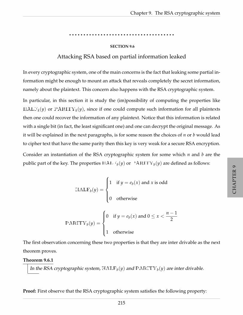
CH

AP

TE

R9

CH

AP

TE

R9

CH

AP

TE

R9

CH

AP

TE

R9

CH

AP

TE

R9

CH

AP

TE

R9

CH

AP

TE

R9

CH

AP

TE

R9


• • • • • • • • • • • • • • • • • • • • • • • • • • • • • • • • • • • • •

SECTION 9.6

Attacking RSA based on partial information leaked

In every cryptographic system, one of the main concerns is the fact that leaking some partial in-

formation might be enough to mount an attack that reveals completely the secret information,

namely about the plaintext. This concern also happens with the RSA cryptographic system.

In particular, in this section it is study the (im)possibility of computing the properties like

HALFk(y) or PARITYk(y), since if one could compute such information for all plaintexts

then one could recover the information of any plaintext. Notice that this information is related

with a single bit (in fact, the least significant one) and one can decrypt the original message. As

it will be explained in the next paragraphs, is for some reason the choices of n or b would lead

to cipher text that have the same parity then this key is very weak for a secure RSA encryption.

Consider an instantiation of the RSA cryptographic system for some which n and b are the

public part of the key. The properties HALFb(y) or PARITYb(y) are defined as follows:

HALFb(y) =

1 if y = eb(x) and x is odd

0 otherwise

PARITYb(y) =

0 if y = eb(x) and 0 ≤ x <

n− 12

1 otherwise

The first observation concerning these two properties is that they are inter drivable as the next

theorem proves.

Theorem 9.6.1

In the RSA cryptographic system, HALFb(y) and PARITYb(y) are inter drivable.

Proof: First observe that the RSA cryptographic system satisfies the following property:

215

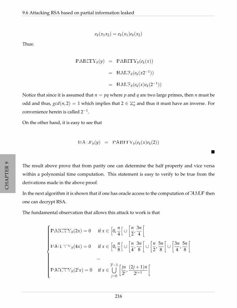
CH

AP

TE

R9

CH

AP

TE

R9

CH

AP

TE

R9

CH

AP

TE

R9

CH

AP

TE

R9

CH

AP

TE

R9

CH

AP

TE

R9

CH

AP

TE

R9

9.6 Attacking RSA based on partial information leaked

eb(x1x2) = eb(x1)eb(x2)

Thus:

PARITYb(y) = PARITYb(ek(x))

= HALFb(ek(x2−1))

= HALFb(ek(x)ek(2−1))

Notice that since it is assumed that n = pq where p and q are two large primes, then n must be

odd and thus, gcd(n, 2) = 1 which implies that 2 ∈ Z∗n and thus it must have an inverse. For

convenience herein is called 2−1.

On the other hand, it is easy to see that

HALFb(y) = PARITYb(ek(x)ek(2))

The result above prove that from parity one can determine the half property and vice versa

within a polynomial time computation. This statement is easy to verify to be true from the

derivations made in the above proof.

In the next algorithm it is shown that if one has oracle access to the computation ofHALF then

one can decrypt RSA.

The fundamental observation that allows this attack to work is that

PARITYb(2x) = 0 if x ∈[0,

n4

[∪[

n2

,3n4

[

PARITYb(4x) = 0 if x ∈[0,

n8

[∪[

n4

,3n8

[∪[

n2

,5n8

[∪[

3n4

,5n8

[...

PARITYb(2ix) = 0 if x ∈2i−1⋃j=0

[jn2i ,

(2j + 1)n2i+1

[

216

CH

AP

TE

R9

CH

AP

TE

R9

CH

AP

TE

R9

CH

AP

TE

R9

CH

AP

TE

R9

CH

AP

TE

R9

CH

AP

TE

R9

CH

AP

TE

R9


Algorithm 9.6.1 (Decrypting RSA based on an oracle forHALF)

Input y, n and b such that y = eb(x), where eb is the RSA encryption function with

public part n and b;

Output x;

Oracle HALF;

Step 1 For i = 0 toblog2 nc do

Step 1.1 yi = HALFb(y);

Step 1.2 y = y · eb(2) (mod n) = y · 2b (mod n);

Step 2 l = 0;

Step 3 h = n;

Step 4 For i = 0 toblog2 nc do

Step 4.1 m = (h− l)/2;

Step 4.2 If yi = 1 then l = m else h = m;

Step 5 Output bhc;

The read is invited to prove that if HALF is polynomial then, the algorithm presented above

runs in polynomial time and, in fact, the value outputted is just the plaintext.

This example shows the fragility of RSA if the parity of the messages can be computed easily. It

is worthwhile mention that there are also other kinds of information of the plaintexts that one

opponent can use to attack the RSA cryptographic system and each of them require a separated

proof of security.

217

CH

AP

TE

R9

CH

AP

TE

R9

CH

AP

TE

R9

CH

AP

TE

R9

CH

AP

TE

R9

CH

AP

TE

R9

CH

AP

TE

R9

CH

AP

TE

R9

9.7 The Rabin’s cryptographic system and its relationship with RSA

• • • • • • • • • • • • • • • • • • • • • • • • • • • • • • • • • • • • •

SECTION 9.7

The Rabin’s cryptographic system and its relationship with

RSA

In this section, it described the Rabin’s cryptographic system and explored its connection to

RSA. This cryptographic system was presented in 1979 by Michael Rabin, in an effort to im-

prove the RSA cryptographic system. This system is also an asymmetric cryptographic system

which security relies on the difficulty of factorization. In fact, the remarkable point of this

system is that it has the advantage that the problem on which it relies has been mathematically

proved to be as hard as integer factorization while this is not known to be true for the RSA

problem. I.e., even if factorization is not P then no one knows if RSA is not insecure. In fact,

it is very well known that it possible, in theory, that breaking RSA does not necessarily mean

that one has to determine p and q in polynomial time, i.e., one may have factorization problem

not being a problem in P but the RSA being insecure. This issue was already realized in the

original paper of Rivest, Shamir and Adleman that stated the following sentence:

It may be possible to prove that any general method of breaking our scheme yields an efficient

factoring algorithm. This would establish that any way of breaking our scheme must be as

difficult as factoring. We have not been able to prove this conjecture.

The difficulties involved on proving this conjecture can be seen in the following way. If one

could show that from a ciphertext y and its corresponding plaintext x one would be able to

compute the factors p and q, then one could, in particular, factorize n by choosing any other

message x′ and its corresponding ciphertext y = ek(x) and then compute p and q using the

presumed to exist procedure, giving a polynomial time algorithm for Factorization, which is

not known to exist.

As it will be discussed on this section, the Rabin Cryptographic system, is an example of com-

putable provably secure scheme against chosen-plaintext attacks provided that the modulus

n = pq cannot be factored efficiently. Although it is not used in practice for technical reasons

218

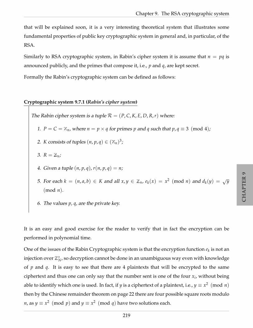
CH

AP

TE

R9

CH

AP

TE

R9

CH

AP

TE

R9

CH

AP

TE

R9

CH

AP

TE

R9

CH

AP

TE

R9

CH

AP

TE

R9

CH

AP

TE

R9


that will be explained soon, it is a very interesting theoretical system that illustrates some

fundamental properties of public key cryptographic system in general and, in particular, of the

RSA.

Similarly to RSA cryptographic system, in Rabin’s cipher system it is assume that n = pq is

announced publicly, and the primes that compose it, i.e., p and q, are kept secret.

Formally the Rabin’s cryptographic system can be defined as follows:

Cryptographic system 9.7.1 (Rabin’s cipher system)

The Rabin cipher system is a tupleR = (P, C, K, E, D, R, r) where:

1. P = C = Zn, where n = p× q for primes p and q such that p, q ≡ 3 (mod 4);

2. K consists of tuples (n, p, q) ∈ (Zn)3;

3. R = Zn;

4. Given a tuple (n, p, q), r(n, p, q) = n;

5. For each k = (n, a, b) ∈ K and all x, y ∈ Zn, ek(x) = x2 (mod n) and dk(y) =√

y

(mod n).

6. The values p, q, are the private key.

It is an easy and good exercise for the reader to verify that in fact the encryption can be

performed in polynomial time.

One of the issues of the Rabin Cryptographic system is that the encryption function ek is not an

injection over Z∗N, so decryption cannot be done in an unambiguous way even with knowledge

of p and q. It is easy to see that there are 4 plaintexts that will be encrypted to the same

ciphertext and thus one can only say that the number sent is one of the four xi, without being

able to identify which one is used. In fact, if y is a ciphertext of a plaintext, i.e., y ≡ x2 (mod n)

then by the Chinese remainder theorem on page 22 there are four possible square roots modulo

n, as y ≡ x2 (mod p) and y ≡ x2 (mod q) have two solutions each.

219

CH

AP

TE

R9

CH

AP

TE

R9

CH

AP

TE

R9

CH

AP

TE

R9

CH

AP

TE

R9

CH

AP

TE

R9

CH

AP

TE

R9

CH

AP

TE

R9


In practice, this is not serious, since it is very unlikely that more than one of the xi would

correspond to a real meaningful message. Another way to avoid this issue, and that will be

explained below, is to consider only plaintexts that are themselves quadratic residues.

Notice that if p and q are known, it is easy to compute all the xi such that ek(xi) = y and the

knowledge of n, y and all the xi, one can compute p, q. On the other hand, one is not able to

obtain p and q from just one of the xi efficiently, so the approach based on x and ek(x) described

above does not work in polynomial time. Moreover, n being composite implies that, as far as it

is known in practice, an opponent cannot invert the encryption fast, i.e., without knowing the

prime factors p and q then computing the square roots (to recover the original message) cannot

be done in polynomial time. Hence the security of this system relies on the impossibility of fast

computation of square roots modulo composite numbers.

From the decryption point of view, notice that the choices of the primes being congruents with

3 modulo 4 it is not really a requirement since the computation of the square roots of a number

modulo primes can be done in polynomial time. Although this choice allows a faster way of

decryption. Since p, q ≡ 3 (mod 4), then there are integer k1 and k2 such that 4k1 = p + 1 and

4k2 = q + 1 and thus, in particular (p + 1)/4 and (p + 1)/4 are integers.

Thus, if y1 ≡ y mod p and y2 ≡ y mod q then x ≡ y1k1 (mod p) and x ≡ y2

k2 (mod q). In

fact if x1 ≡ y1k1 (mod p) and x2 ≡ y2

k2 (mod q) by Euler’s Theorem 2.3.6 on Page 2.3.6 one

has:

x12 ≡ (y1

k1)2 ≡ (x2k1)2 (mod p)

≡ x4k1 ≡ xp+1 (mod p)

≡ xp−1x2 ≡ x2 (mod p)

and similarly

x22 ≡ (y2

k2)2 ≡ (x2k2)2 (mod p)

≡ x4k2 ≡ xq+1

≡ xq−1x2 ≡ x2 (mod q).

220

CH

AP

TE

R9

CH

AP

TE

R9

CH

AP

TE

R9

CH

AP

TE

R9

CH

AP

TE

R9

CH

AP

TE

R9

CH

AP

TE

R9

CH

AP

TE

R9


Then all the solutions of the equations above arez1 ≡ x1 (mod p)

z1 ≡ x2 (mod q)

z2 ≡ x1 (mod p)

z2 ≡ −x2 (mod q)

z3 ≡ −x1 (mod p)

z3 ≡ x2 (mod q)

z4 ≡ −x1 (mod p)

z4 ≡ −x2 (mod q)

Thus, using the Chinese remainder theorem on page 22 one can recover all possible original

messages very efficiently using the above equations. On the other hand, as stated above, if the

original messages are themselves quadratic residues then the decryption process can be done

unique. In fact if x is a quadratic residue then there exists s ∈ Z∗n such that s2 ≡ x (mod n) and

thus:

y1k1 ≡ (x2)k1 ≡ (s4)k1 (mod p)

≡ sp+1 ≡ sp−1s2 (mod p)

≡ s2 ≡ x (mod p)

and similarly

y2k2 ≡ (x2)k2 ≡ (s4)k2 (mod q)

≡ sp+1 ≡ sp−1s2 (mod p)

≡ s2 ≡ x (mod q).

and again by the Chinese remainder theorem on page 22 one can recover x (mod n).

In the discussion above it was mentioned that the security of Rabin’s cryptographic scheme is

equivalent to Factorization. This means that a probabilistic polynomial algorithm for break-

ing the Rabin’s cryptographic scheme can be used to obtain a polynomial time algorithm for

Factorization and vice versa.

Clearly, if one has access to an oracle for factoring numbers then, using the above description

one can determine the square roots modulo n and thus one can break the Rabin’s cryptographic

221

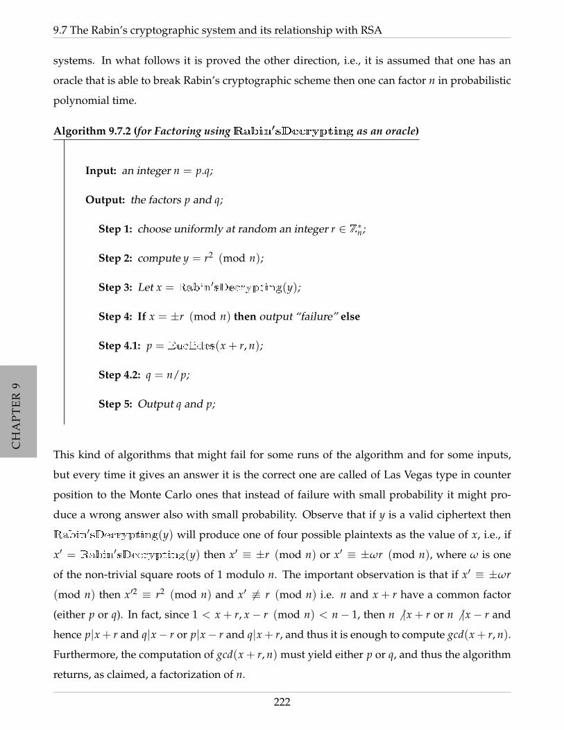
CH

AP

TE

R9

CH

AP

TE

R9

CH

AP

TE

R9

CH

AP

TE

R9

CH

AP

TE

R9

CH

AP

TE

R9

CH

AP

TE

R9

CH

AP

TE

R9


systems. In what follows it is proved the other direction, i.e., it is assumed that one has an

oracle that is able to break Rabin’s cryptographic scheme then one can factor n in probabilistic

polynomial time.

Algorithm 9.7.2 (for Factoring usingRabin′sDecrypting as an oracle)

Input: an integer n = p.q;

Output: the factors p and q;

Step 1: choose uniformly at random an integer r ∈ Z∗n;

Step 2: compute y = r2 (mod n);

Step 3: Let x = Rabin′sDecrypting(y);

Step 4: If x = ±r (mod n) then output “failure” else

Step 4.1: p = Euclides(x + r, n);

Step 4.2: q = n/p;

Step 5: Output q and p;

This kind of algorithms that might fail for some runs of the algorithm and for some inputs,

but every time it gives an answer it is the correct one are called of Las Vegas type in counter

position to the Monte Carlo ones that instead of failure with small probability it might pro-

duce a wrong answer also with small probability. Observe that if y is a valid ciphertext then

Rabin′sDecrypting(y) will produce one of four possible plaintexts as the value of x, i.e., if

x′ = Rabin′sDecrypting(y) then x′ ≡ ±r (mod n) or x′ ≡ ±ωr (mod n), where ω is one

of the non-trivial square roots of 1 modulo n. The important observation is that if x′ ≡ ±ωr

(mod n) then x′2 ≡ r2 (mod n) and x′ 6≡ r (mod n) i.e. n and x + r have a common factor

(either p or q). In fact, since 1 < x + r, x− r (mod n) < n− 1, then n 6 |x + r or n 6 |x− r and

hence p|x + r and q|x− r or p|x− r and q|x + r, and thus it is enough to compute gcd(x + r, n).

Furthermore, the computation of gcd(x + r, n) must yield either p or q, and thus the algorithm

returns, as claimed, a factorization of n.

222

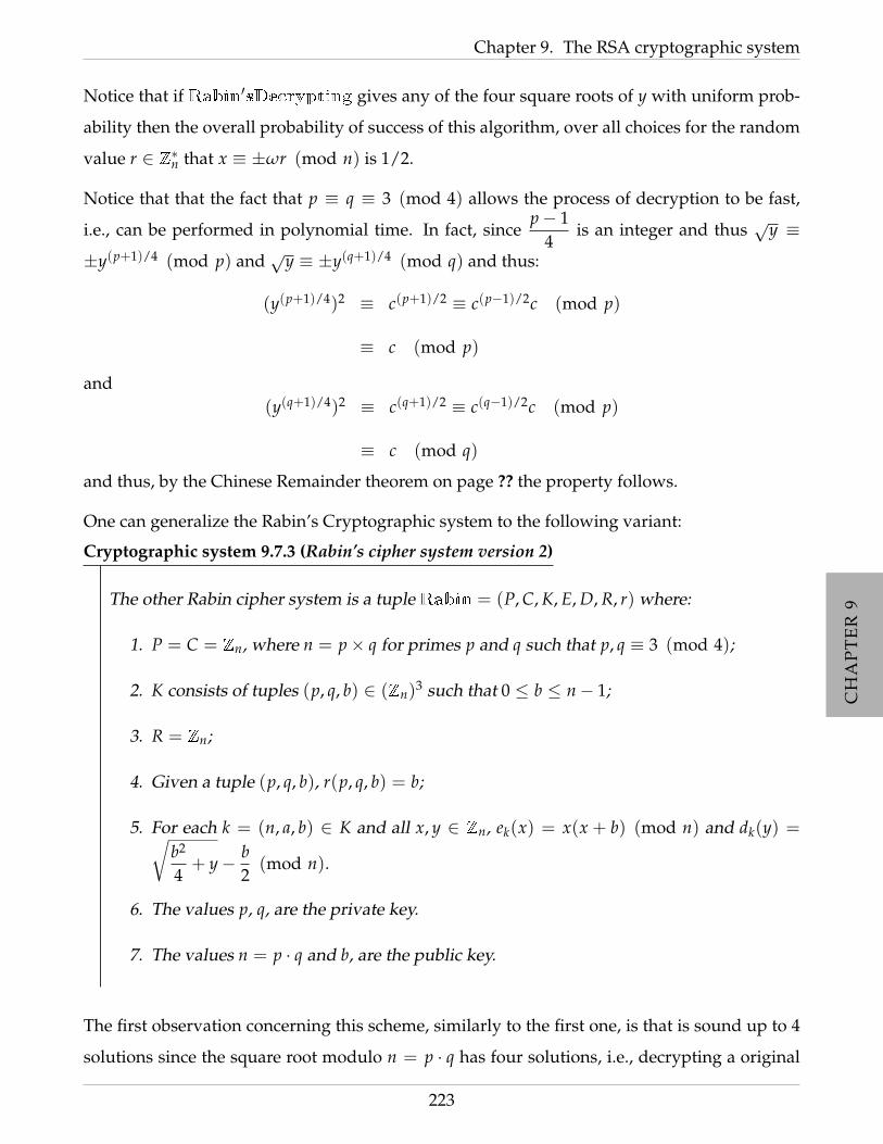
CH

AP

TE

R9

CH

AP

TE

R9

CH

AP

TE

R9

CH

AP

TE

R9

CH

AP

TE

R9

CH

AP

TE

R9

CH

AP

TE

R9

CH

AP

TE

R9


Notice that if Rabin′sDecrypting gives any of the four square roots of y with uniform prob-

ability then the overall probability of success of this algorithm, over all choices for the random

value r ∈ Z∗n that x ≡ ±ωr (mod n) is 1/2.

Notice that that the fact that p ≡ q ≡ 3 (mod 4) allows the process of decryption to be fast,

i.e., can be performed in polynomial time. In fact, sincep− 1

4is an integer and thus

√y ≡

±y(p+1)/4 (mod p) and√

y ≡ ±y(q+1)/4 (mod q) and thus:

(y(p+1)/4)2 ≡ c(p+1)/2 ≡ c(p−1)/2c (mod p)

≡ c (mod p)

and(y(q+1)/4)2 ≡ c(q+1)/2 ≡ c(q−1)/2c (mod p)

≡ c (mod q)

and thus, by the Chinese Remainder theorem on page ?? the property follows.

One can generalize the Rabin’s Cryptographic system to the following variant:

Cryptographic system 9.7.3 (Rabin’s cipher system version 2)

The other Rabin cipher system is a tuple Rabin = (P, C, K, E, D, R, r) where:

1. P = C = Zn, where n = p× q for primes p and q such that p, q ≡ 3 (mod 4);

2. K consists of tuples (p, q, b) ∈ (Zn)3 such that 0 ≤ b ≤ n− 1;

3. R = Zn;

4. Given a tuple (p, q, b), r(p, q, b) = b;

5. For each k = (n, a, b) ∈ K and all x, y ∈ Zn, ek(x) = x(x + b) (mod n) and dk(y) =√b2

4+ y− b

2(mod n).

6. The values p, q, are the private key.

7. The values n = p · q and b, are the public key.

The first observation concerning this scheme, similarly to the first one, is that is sound up to 4

solutions since the square root modulo n = p · q has four solutions, i.e., decrypting a original

223

CH

AP

TE

R9

CH

AP

TE

R9

CH

AP

TE

R9

CH

AP

TE

R9

CH

AP

TE

R9

CH

AP

TE

R9

CH

AP

TE

R9

CH

AP

TE

R9


message that was properly encrypted with Rabin’s system then it leads to a original message

that is one of the four possible messages.

In the next lemma it is formally proved this aspect of this system.

Lemma 9.7.4. Let n = p× q be such that p and q. Then equation x2 ≡ 1 (mod n) has 4 solutions

modulo n.

Proof: Notice that, by the Chinese Remainder theorem 2.3.4:

x2 ≡ 1 (mod n) ⇔ x2 − 1 ≡ 0 (mod n)

⇔

x2 ≡ 1 (mod p)

x2 ≡ 1 (mod q)

⇔

x ≡ ±1 (mod p)

x ≡ ±1 (mod q)

Thus, reverting the Chinese Remainder theorem 2.3.4 x2 ≡ 1 (mod n) has the solutions 1, −1

and ω, a non trivial solution that in fact results from the above mentioned theorem for the case:

x ≡ 1 (mod p)

x ≡ −1 (mod q)

Lemma 9.7.5. Let ek be the encryption function of Rabin’s cipher system version 2 described in the

Cryptographic system 9.7.3. Then ek is not injective.

Proof: Assume that ek(x) = x(x + b) (mod n). Then:

224

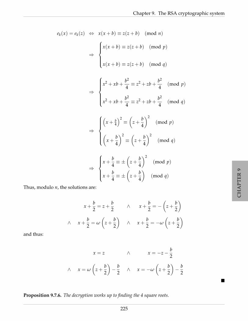
CH

AP

TE

R9

CH

AP

TE

R9

CH

AP

TE

R9

CH

AP

TE

R9

CH

AP

TE

R9

CH

AP

TE

R9

CH

AP

TE

R9

CH

AP

TE

R9


ek(x) = ek(z) ⇔ x(x + b) ≡ z(z + b) (mod n)

⇒

x(x + b) ≡ z(z + b) (mod p)

x(x + b) ≡ z(z + b) (mod q)

⇒

x2 + xb +

b2

4≡ z2 + zb +

b2

4(mod p)

x2 + xb +b2

4≡ z2 + zb +

b2

4(mod q)

⇒

(x + b

4

)2≡(

z +b4

)2

(mod p)

(x +

b4

)2

≡(

z +b4

)2

(mod q)

⇒

x +

b4≡ ±

(z +

b4

)2

(mod p)

x +b4≡ ±

(z +

b4

)(mod q)

Thus, modulo n, the solutions are:

x +b2= z +

b2

∧ x +b2= −

(z +

b2

)

∧ x +b2= ω

(z +

b2

)∧ x +

b2= −ω

(z +

b2

)and thus:

x = z ∧ x = −z− b2

∧ x = ω

(z +

b2

)− b

2∧ x = −ω

(z +

b2

)− b

2

Proposition 9.7.6. The decryption works up to finding the 4 square roots.

225

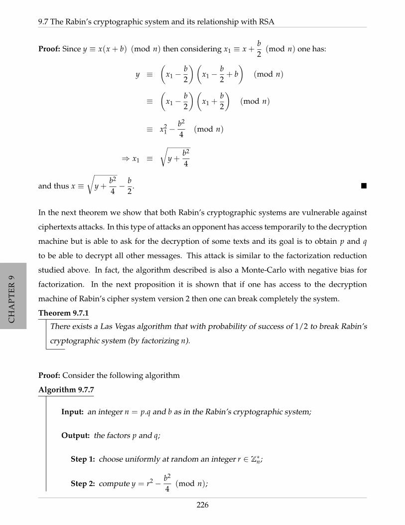
CH

AP

TE

R9

CH

AP

TE

R9

CH

AP

TE

R9

CH

AP

TE

R9

CH

AP

TE

R9

CH

AP

TE

R9

CH

AP

TE

R9

CH

AP

TE

R9


Proof: Since y ≡ x(x + b) (mod n) then considering x1 ≡ x +b2

(mod n) one has:

y ≡(

x1 −b2

)(x1 −

b2+ b)

(mod n)

≡(

x1 −b2

)(x1 +

b2

)(mod n)

≡ x21 −

b2

4(mod n)

⇒ x1 ≡√

y +b2

4

and thus x ≡√

y +b2

4− b

2.

In the next theorem we show that both Rabin’s cryptographic systems are vulnerable against

ciphertexts attacks. In this type of attacks an opponent has access temporarily to the decryption

machine but is able to ask for the decryption of some texts and its goal is to obtain p and q

to be able to decrypt all other messages. This attack is similar to the factorization reduction

studied above. In fact, the algorithm described is also a Monte-Carlo with negative bias for

factorization. In the next proposition it is shown that if one has access to the decryption

machine of Rabin’s cipher system version 2 then one can break completely the system.

Theorem 9.7.1

There exists a Las Vegas algorithm that with probability of success of 1/2 to break Rabin’s

cryptographic system (by factorizing n).

Proof: Consider the following algorithm

Algorithm 9.7.7

Input: an integer n = p.q and b as in the Rabin’s cryptographic system;

Output: the factors p and q;

Step 1: choose uniformly at random an integer r ∈ Z∗n;

Step 2: compute y = r2 − b2

4(mod n);

226

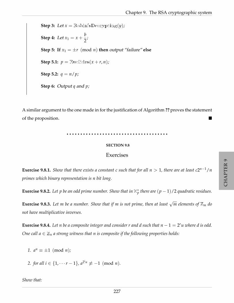
CH

AP

TE

R9

CH

AP

TE

R9

CH

AP

TE

R9

CH

AP

TE

R9

CH

AP

TE

R9

CH

AP

TE

R9

CH

AP

TE

R9

CH

AP

TE

R9


Step 3: Let x = Rabin′sDecrypting(y);

Step 4: Let x1 = x +b2

;

Step 5: If x1 = ±r (mod n) then output “failure” else

Step 5.1: p = Euclides(x + r, n);

Step 5.2: q = n/p;

Step 6: Output q and p;

A similar argument to the one made in for the justification of Algorithm ?? proves the statement

of the proposition.

• • • • • • • • • • • • • • • • • • • • • • • • • • • • • • • • • • • • •

SECTION 9.8

Exercises

Exercise 9.8.1. Show that there exists a constant c such that for all n > 1, there are at least c2n−1/n

primes which binary representation is n bit long.

Exercise 9.8.2. Let p be an odd prime number. Show that in Z∗p there are (p− 1)/2 quadratic residues.

Exercise 9.8.3. Let m be a number. Show that if m is not prime, then at least√

m elements of Zm do

not have multiplicative inverses.

Exercise 9.8.4. Let n be a composite integer and consider r and d such that n− 1 = 2ru where d is odd.

One call a ∈ Zn a strong witness that n is composite if the following properties holds:

1. au ≡ ±1 (mod n);

2. for all i ∈ 1, · · · r− 1, a2iu 6≡ −1 (mod n).

Show that:

227

CH

AP

TE

R9

CH

AP

TE

R9

CH

AP

TE

R9

CH

AP

TE

R9

CH

AP

TE

R9

CH

AP

TE

R9

CH

AP

TE

R9

CH

AP

TE

R9

9.8 Exercises

1. if n is odd that is not a prime power, then at least half the elements of Z∗n that are strong witnesses

that n is composite.

2. one can test in polynomial time if a is a strong witness that n is composite.

Exercise 9.8.5. Let p be an odd prime number. Show that there is only one element in Zp+1 that does

not pass the primality test xm−1 ≡ 1 (mod p + 1), in the case, m = p + 1.

In the next exercise, the reader is invited to simulate the RSA encryption scheme for a simple

case.

Exercise 9.8.6. Assume that one choose p = 11, q = 19 for the RSA cryptographic system. Let (a, b)

be key for this cryptographic system.

1. Prove that one can choose b = 7.

2. Compute the value of a.

3. Show how to encrypt the message 100.

4. Show how to decrypt the resulting message of the previous item.

Exercise 9.8.7. Assume that one choose p = 11, q = 23 for the RSA cryptographic system. Let (a, b)

be key for this cryptographic system.

1. Prove that one can choose b = 7.

2. Compute the value of a.

3. Show how to encrypt the message 100.

4. Show how to decrypt the resulting message of the previous item.

In the next exercise it is studied a variant of the RSA system where instead of assuming that

a and b are chosen to be inverse of each other it is assumed that they are inverse modulo

γ(n) =φ(n)

gcd(φ(p), φ(q)).

Exercise 9.8.8. One can use a simple variation of the RSA cryptographic system as follows:

228

CH

AP

TE

R9

CH

AP

TE

R9

CH

AP

TE

R9

CH

AP

TE

R9

CH

AP

TE

R9

CH

AP

TE

R9

CH

AP

TE

R9

CH

AP

TE

R9


Cryptographic system 9.8.9 (Alternative RSA cipher system)

The cipher system consists of a tuple C = (P, C, K, E, D, R, r) where:

1. P = C = Zn, where n = p× q for primes p and q;

2. K consists of pairs k = (a, b) ∈ (Zn)2 such that a · b ≡ 1 (mod γ(n)), where γ(n) =φ(n)

gcd(φ(p), φ(q)), i.e., a and b are inverse of each order modulo γ(n);

3. R = Zn;


5. For each k = (a, b) ∈ K and all x, y ∈ Zn, ek(x) = xb (mod n) and dk(y) = ya

(mod n).

6. The values n and b form the public key, and p, q, a are the private key.

Show that this scheme is also sound, i.e., decrypting and encrypted message one gets the original

message.

Exercise 9.8.10. Let n be a composite integer that is product of the form pq where p and q are primes.

Show that if φ(n) and n are known then it is possible to compute p and q.

In the next exercise it is introduced the Carmichael function discussed in the section concerning

the AKS algorithm.

Exercise 9.8.11. Let n > 2 be an odd number and letr

∏i=1

peii its prime decomposition. The λ-Carmichael

function is defined by:

λ(n) = lcm(φ(pe11 , · · · , per

r ))

where φ is the Euler function. Prove that:

1. aλ(n) ≡ 1 (mod n) for all a ∈ Z∗n;

2. an−1 ≡ 1 (mod n) if and only if λ(n)|n− 1;

3. Consider Cn = a ∈ Z∗n : aλ(n)/2 ≡ ±1 (mod n). Then, Cn is a multiplicative subgroup of

Z∗n;

229

CH

AP

TE

R9

CH

AP

TE

R9

CH

AP

TE

R9

CH

AP

TE

R9

CH

AP

TE

R9

CH

AP

TE

R9

CH

AP

TE

R9

CH

AP

TE

R9

9.8 Exercises

4. Cn = Z∗n if and only if n = pe with p prime and e > 1.

In the next exercise it is study a variant of the Solovay–Strassen algorithm for primality testing.

Exercise 9.8.12 (Lehmann’s primality test). Let n be an odd integer larger than 3. Denote by f :

Z∗n → Z∗n defined by f (a) = a(n−1)/2. Let E be the range of f . Show that:

1. E = −1, 1 if and only if n is prime.

2. if n is not a prime power then E 6= −1, 1.

3. Show that if n = pe with p prime and e ≥ 2 then E 6= −1, 1.

4. if E = 1, n is a Carmichael number.

5. The Lehmann’s algorithm for primality test is the following:

Algorithm 9.8.13 (Lehmann’s primality test – L)

Input: n an odd integer and an integer t > 0, the number of trials.

Step 1: For n = 1 tot do

Step 1.1: Choose uniformly at random ai ∈ 1, · · · , n− 1.

Step 1.2: Compute bi = a(n−1)/2 (mod n).

Step 2: If b1, · · · , bt 6= −1, 1 then output probably composite

else output probably prime.

Prove the following properties:

(a) if n is prime the probability that the algorithm returns probably prime is at least 1− 21−t.

(b) if n is composite, the probability that the algorithm returns probably composite is at least

1− 2−t.

(c) the complexity of the algorithm is O(t log2 n).

(d) for each of the numbers 343, 561, 667 and 841, compute E and confront with the results of

the previous items.

In the next exercise the reader is asked to redo the proof of Theorem 9.3.7

230

CH

AP

TE

R9

CH

AP

TE

R9

CH

AP

TE

R9

CH

AP

TE

R9

CH

AP

TE

R9

CH

AP

TE

R9

CH

AP

TE

R9

CH

AP

TE

R9


Exercise 9.8.14. Let n be an odd integer and consider the following subset of Z∗n:

E(n) =

a ∈ Z∗n :( a

n

)≡ a(n−1)/2 (mod n)

1. Prove that E(n) is a subgroup of Z∗n.

2. Prove that if n = pkq where p is a prime number with k ≥ 2 and gcd(p, q) = 1 then G(n) ( Z∗n,

i.e, there is an a ∈ Z∗n such that( a

n)6≡ a(n−1)/2 (mod n). (Hint: consider the element a =

pk−1q + 1 and its binomial expansion)

3. Assume now that n = pq where p and q are distinct primes.

(a) Show that there exists a ∈ Z∗n such that a is not a quadratic residue modulo p and a ≡ 1

(mod q). (hint: use the Chinese remainder theorem).

(b) Show that such a is not an element of G(n) (hint: show that( a

n

)6≡ −1 (mod n) and

a(n−1)/2 6≡ −1 (mod n))

4. Prove that the same properties of the previous item hold if n = p1 · · · pl where pi are all distinct

odd primes.

5. Prove that if n is composite and odd then ord(G(n)) ≤ n− 12

.

6. From the previous item conclude that the Solovay–Strassen Algorithm SS presented in Algorithm

9.3.9 is indeed a Monte-Carlo one with bias one half.

7. Discuss why in the previous items the question of n being even is ruled out of the discussion.

Exercise 9.8.15. Recall that one says that an encryption scheme is secure against chosen-ciphertext

attacks if even one opponent having access to the decryption process on messages different from the

original one it cannot recover the original message.

Show that the RSA cryptographic system is not secure against this type of attacks by showing a way

that an opponent can use to decrypt a message.

Exercise 9.8.16. exercise 5.18 in [?] One says that a plaintext is fixed if ek(x) = x. Show that the RSA

cryptographic system has gcd(b− 1, p− 1) · gcd(b− 1, q− 1) fixed plain texts in Z∗n .

In the next exercises it is shown that despite the fact one has a presumably secure encryption

scheme a sloppy use of it can compromise its security.

231

CH

AP

TE

R9

CH

AP

TE

R9

CH

AP

TE

R9

CH

AP

TE

R9

CH

AP

TE

R9

CH

AP

TE

R9

CH

AP

TE

R9

CH

AP

TE

R9

9.8 Exercises

Exercise 9.8.17. Common modulus Assume that two users of the RSA cryptographic system A1 and

A2 have as public keys, respectively (n, b1) and (n, b2) with gcd(b1, b2) = 1, i.e., they share the same

modulus but with different encryption exponents. Suppose that a third party S wishes to send the same

message x to both A1 and A2 using their encryption exponent.

1. Show how an opponent O one can easily obtain the original message if it intersects both encrypted

messages. (hint: use the Euclides algorithm).

2. Another way of decrypting the message is to consider the following algorithm:

Algorithm 9.8.18

Input: n, b1, b2, y1 = xb1 and y2 = xb2 .

Step 1: c1 = b−11 (mod b2);

Step 2: c2 = (c1b1 − 1)div b2;

Step 3: x1 = yc11 (yc2

2 )−1;

Show that in fact x1 ≡ x (mod n);

Exercise 9.8.19 (small exponent attack). The public exponent b in the RSA Cryptographic system can

be chosen arbitrarily as long as gcd(b, φ(n)) = 1 but usually the users tend to choose small exponents

to speed up the encryption process. Assume that three users A1, A2 and A3 such that their public keys

are, respectively, (n1, 3), (n2, 3) and (n3, 3).

Show that it is reasonable to assume that n1, n2 and n3 are all different and also that the pairwise greatest

common divisor of them is equal to 1.

Assume that n1, n2 and n3 are all different and they are pairwise co-primes and consider another party

C that wants to send a message x to all of them using the RSA Cryptographic system with their public

key. Show that an opponent that intercepts the three encrypted messages can decrypt them and recover

the original message.

This attack takes advantage of the low exponent 3 but can be performed with other small exponents.

Explain how this attack can be performed in practice.

232

CH

AP

TE

R9

CH

AP

TE

R9

CH

AP

TE

R9

CH

AP

TE

R9

CH

AP

TE

R9

CH

AP

TE

R9

CH

AP

TE

R9

CH

AP

TE

R9


In the next exercise the reader is asked to check that even if p and q are chosen to be congruent

with 5 modulo 8 then one can perform square roots in polynomial time. This is an important

observation concerning Rabin’s cryptographic system.

Exercise 9.8.20 (square roots modulo p ≡ 5 (mod 8)). Let p be an odd prime number such that

p ≡ 5 (mod 8). Let a be a quadratic residue modulo p.

1. Show that 4|p− 1 and 8|p + 3;

2. Envisage the values of a(p?1)/4;

3. Compute the value 4(p−1)/4.

4. Consider the following algorithm to compute the square root:

Algorithm 9.8.21

Input an odd prime p such that p ≡ 5 (mod 8) and a quadratic residue a.

Output a square root of a modulo p.

Step 1 Compute the value d = a(p−1)/4 (mod p).

Step 2 If d = 1 then compute r = a(p+3)/8 (mod p)

else r = 2a(4a)(p−5)/8 (mod p).

Step 3 Output r.

Prove that in fact the value retrieved by the algorithm is a square root of a.

5. Prove that the algorithm runs in polynomial time.

233

CH

AP

TE

R9

CH

AP

TE

R9

CH

AP

TE

R9

CH

AP

TE

R9

CH

AP

TE

R9

CH

AP

TE

R9

CH

AP

TE

R9

CH

AP

TE

R9

9.8 Exercises

234

CH

AP

TE

R10

CH

AP

TE

R10

CH

AP

TE

R10

CH

AP

TE

R10

CH

AP

TE

R10

CH

AP

TE

R10

CH

AP

TE

R10

CH

AP

TE

R10

CH

AP

TE

R10

CHAPTER 10

Cryptographic schemes based on the

discrete logarithmic problem

In this chapter it is studied the problem of discrete logarithm and some of its applications to

cryptography. Heuristically speaking, this problem consists on finding the smallest exponent

that one has to power a given number (usually a generator of a finite group) to obtain a target

element. Similarly to the problem of determining the square roots, which is simple in N but

presumably hard when moduli are considered, the discrete logarithm also shares similar prop-

erties. The hardness of this problem is the base of security of many cryptographic schemes such

as Diffie–Hellman key agreement, ElGamal encryption and the ElGamal signature scheme. It

will also be discussed the Pohling–Hellman algorithm.

• • • • • • • • • • • • • • • • • • • • • • • • • • • • • • • • • • • • •

SECTION 10.1

The discrete logarithmic problem

As discussed in the basic material part of these notes one important question is the construction

of easy to compute functions that are presumably hard to invert. One of those functions is

constructed based on the following problem:

235

CH

AP

TE

R10

CH

AP

TE

R10

CH

AP

TE

R10

CH

AP

TE

R10

CH

AP

TE

R10

CH

AP

TE

R10

CH

AP

TE

R10

CH

AP

TE

R10

CH

AP

TE

R10

10.1 The discrete logarithmic problem

Problem 10.1.1 (Discrete logarithm over a finite group -Discrete Logarithm)

Let (G, ·) be an Abelian group and consider two elements g ∈ G and h such that g has order

n and h ∈ 〈g〉, i.e., h is an element in the subgroup generated by g.

Instance: G, g and h as described above and n = ord(g).

Question: Find the unique integer 0 < a < n− 1 such that and gn = h?

It is common to denote a by logg h, since by analogy to the logarithmic function in R, the value

a is defined to be the logarithm of h on base g since it is the least number that one has to power

g to obtain h. Since the values are taken modulo n, the adopted name perfectly describes the

problem. One common choice for G is some (Z∗p,×) where p is a prime and g is a generator of

the group. Another one is to consider g = ω a nontrivial lth roots of unity. Even another choice

is to take g to be an element with prime order q, being in latter one the most fruitful choice.

In the next exercise the reader is asked to prove that this problem is a NP problem.

Example 10.1.2. Let (G, ·) be an Abelian group and consider two elements g ∈ G and h such that g

has order n and h ∈ 〈g〉. Prove that the discrete logarithm problem over G described above is NP i.e.,

Discrete Logarithm ∈ NP.

Notice that computing the discrete logarithms is believed to be hard, since no one knows

a polynomial time algorithm to compute it. The reader may think for a while about this

question and how one could compute it in polynomial time. It is also an important open

question/problem in Computer Science. Once the reader is convinced of the hardness of this

problem in a group G then one can use it to give a strong evidence for the fact that the function

f : Z→ G

n 7→ n · g

for g ∈ G is likely to be a one-way function. In the discussion above it was suggested that one

could consider a group Zp with p prime, q to be a prime factor of p− 1 and g to be a nontrivial

lth root of the unity, say g = ω and in fact the difficulty of finding a such that ω2 = ωa where ω

is an element in the subgroup generated by ω relies crucially on the assumption that to solve

a discrete logarithm in this subgroup is essentially equivalent to solve a discrete logarithm in

Z∗q .

236

CH

AP

TE

R10

CH

AP

TE

R10

CH

AP

TE

R10

CH

AP

TE

R10

CH

AP

TE

R10

CH

AP

TE

R10

CH

AP

TE

R10

CH

AP

TE

R10

CH

AP

TE

R10

Chapter 10. Cryptographic schemes based on the discrete logarithmic problem

So, from the argument above one can conclude that, until the writing of this noted, the only

know ways to attack the discrete logarithm directly in the cyclic subgroup is to use generic

methods which all have exponential or subexponential complexity on the length of the order

of the subgroup. For that reason, the standard for Digital Signature established by NIST

recommends the choice of l to be of 160 bit and q to be of size about 1000 bit such that l|q− 1.

It is worthwhile mention that Shoup has proven that the use only of algorithms that use only

properties of operations of the group then the computation of discrete logarithm in a group

of prime order l can not be solved in less than O(√

l) operations, and thus the most effective

methods to solve the discrete logarithm problem in finite fields have to use of extra information

about relations in the group.

This problem and some of its instances can be used in cryptography. For example this problem

is used in the following situations:

• Considering a multiplicative group of a finite field Fq to establish keys agreement, first

proposed by Diffie and Hellman.

• The discrete logarithm in the group of rational points of an elliptic curve over a finite

field Fq to develop cryptographic systems, simultaneously and independently proposed

by Koblitz and Miller in middle of 80’s in two different and independent works.

• • • • • • • • • • • • • • • • • • • • • • • • • • • • • • • • • • • • •

SECTION 10.2

The ElGamal Public-key Cryptographic system

This cryptographic system was proposed by Taher Elgamal in 1984 as a scheme for a public-key

cryptosystem based on the Discrete Logarithm problem in (Z∗p,×).

For sake of understanding it is now lightly explained this encryption scheme. Assume that α

is the generator and β = αa where a is the private key. The plaintext x is transformed into a

ciphertext by multiplying it with βk. The value k can be retrieved by the information of αk that

is also incorporated in the ciphertext. From the decryption point of view, since the private key

a is known one can compute βk using αk and then recovering x by dividing by βk the chipertext.

Formally the ElGamal Public-key Cryptographic System is defined as follows.

237

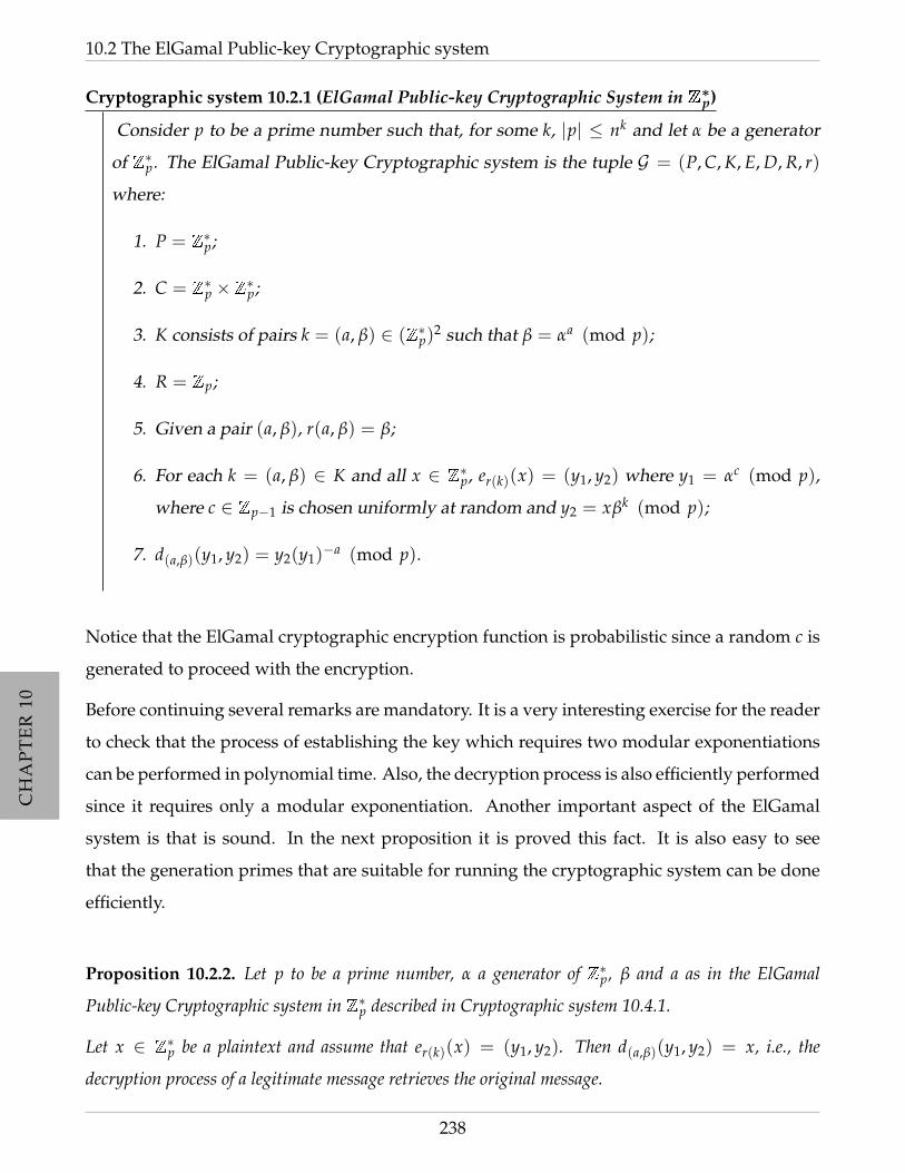
CH

AP

TE

R10

CH

AP

TE

R10

CH

AP

TE

R10

CH

AP

TE

R10

CH

AP

TE

R10

CH

AP

TE

R10

CH

AP

TE

R10

CH

AP

TE

R10

CH

AP

TE

R10

10.2 The ElGamal Public-key Cryptographic system

Cryptographic system 10.2.1 (ElGamal Public-key Cryptographic System in Z∗p)

Consider p to be a prime number such that, for some k, |p| ≤ nk and let α be a generator

of Z∗p. The ElGamal Public-key Cryptographic system is the tuple G = (P, C, K, E, D, R, r)

where:

1. P = Z∗p;

2. C = Z∗p ×Z∗p;

3. K consists of pairs k = (a, β) ∈ (Z∗p)2 such that β = αa (mod p);

4. R = Zp;

5. Given a pair (a, β), r(a, β) = β;

6. For each k = (a, β) ∈ K and all x ∈ Z∗p, er(k)(x) = (y1, y2) where y1 = αc (mod p),

where c ∈ Zp−1 is chosen uniformly at random and y2 = xβk (mod p);

7. d(a,β)(y1, y2) = y2(y1)−a (mod p).

Notice that the ElGamal cryptographic encryption function is probabilistic since a random c is

generated to proceed with the encryption.

Before continuing several remarks are mandatory. It is a very interesting exercise for the reader

to check that the process of establishing the key which requires two modular exponentiations

can be performed in polynomial time. Also, the decryption process is also efficiently performed

since it requires only a modular exponentiation. Another important aspect of the ElGamal

system is that is sound. In the next proposition it is proved this fact. It is also easy to see

that the generation primes that are suitable for running the cryptographic system can be done

efficiently.

Proposition 10.2.2. Let p to be a prime number, α a generator of Z∗p, β and a as in the ElGamal

Public-key Cryptographic system in Z∗p described in Cryptographic system 10.4.1.

Let x ∈ Z∗p be a plaintext and assume that er(k)(x) = (y1, y2). Then d(a,β)(y1, y2) = x, i.e., the

decryption process of a legitimate message retrieves the original message.

238

CH

AP

TE

R10

CH

AP

TE

R10

CH

AP

TE

R10

CH

AP

TE

R10

CH

AP

TE

R10

CH

AP

TE

R10

CH

AP

TE

R10

CH

AP

TE

R10

CH

AP

TE

R10


Proof:d(a,β)(y1, y2) = y2(y1)

−a (mod p)

= xβk((αk)a)−1 (mod p)

= x(αa)k((αk)a)−1 (mod p)

= x

One can generalize the use of the ElGamal cryptographic system to the case where the entire

group is not considered but, instead, considering the discrete logarithm over a subgroup of G

generated by and element α. The idea is that if H = 〈α〉 has high order then computing the

discrete logarithm over H is also hard as it was discussed previously when it was presented the

problem of discrete logarithm. The Generalized ElGamal cryptographic system is then defined

as follows:

Cryptographic system 10.2.3 (Generalized ElGamal Public-key Cryptographic System)

Consider G to be a group and let H be a cyclic subgroup of G. The Generalized ElGamal

Public-key Cryptographic system is the tuple GG = (P, C, K, E, D, R, r) where:

1. P = G;

2. C = G× G;

3. K consists of tuples k = (α, a, β) such that β = αa in G and α is a generator of H;

4. R = H2;

5. Given a tuple (α, a, β), r(α, a, β) = (α, β);

6. For each k = (α, a, β) ∈ K and all x ∈ G, er(k)(x) = (y1, y2) where y1 = αc (mod p),

where c ∈ Z is chosen at random and y2 = xβk in G;

7. d(α,a,β)(y1, y2) = y2((y1)a)−1 in G.

Notice that if one chooses a group where the operation is just the sum, as for example G =

(Zm,+) then αa = aα and thus if β = aα then a = βα−1 and thus the discrete logarithm in

239

CH

AP

TE

R10

CH

AP

TE

R10

CH

AP

TE

R10

CH

AP

TE

R10

CH

AP

TE

R10

CH

AP

TE

R10

CH

AP

TE

R10

CH

AP

TE

R10

CH

AP

TE

R10

10.3 Attacking the Discrete Logarithm problem

this group is computable in polynomial time. Te same problems appear in the cases where the

function Φ : Z∗p → Zp is effectively computable. Notice that in such morphism Φ(1) = 0 and

Φ(ab) = φ(a) + Φ(b).

Proposition 10.2.4. Let p be a prime number. If the morphism Φ : Z∗p → Zp is effectively computable

in polynomial time, then the discrete logarithmic problem over (Z∗p,+) is in P.

The proof of this result is simple and uses the fact that in this case one can compute logα β in

polynomial time by computing the value Φ(β)Φ(α)−1.

• • • • • • • • • • • • • • • • • • • • • • • • • • • • • • • • • • • • •

SECTION 10.3

Attacking the Discrete Logarithm problem

Similarly to Factorization, if we use the ElGammal cryptographic system in a sloppy way than

the system is not secure. In what follows, it is described some attacks that one can perform

in order to compute the discrete logarithms. One of them is what in number theory is called

the Pohlig–Hellman algorithm sometimes credited as the Silver–Pohlig–Hellman which is an

algorithm for computing discrete logarithms in a multiplicative group whose order is a smooth

integer, i.e., any of its prime factors are small.

This algorithm is used to compute logarithms and takes advantage of the factorization of the

order of the group Z∗p, which is assumed to be

n = p− 1 =k

∏i=1

peii

with pi being distinct primes. If a = logα β, then this algorithm determines ai ≡ a (mod peii ) for

1 ≤ i ≤ r, and then using the the Chinese remainder theorem presented in Page 22 to recover a

(mod n). The idea to compute each integer xi is to determined the digits l0, l1, · · · , lei−1 all less

than pi − 1 such that xi = l0 + l1pi + · · ·+ lei−1pei−1i .

Let then q be a prime number and let c be the maximal exponent of q dividing n i.e., such

that qc|n and qc+1 6 |n. Thus, the crucial observation is that a = x + sqc for some integer s.

In particular a = ∑c−1i=0 aiqi + sqc. The next lemma gives gives an idea how the algorithm can

compute a0.

240

CH

AP

TE

R10

CH

AP

TE

R10

CH

AP

TE

R10

CH

AP

TE

R10

CH

AP

TE

R10

CH

AP

TE

R10

CH

AP

TE

R10

CH

AP

TE

R10

CH

AP

TE

R10


Lemma 10.3.1. Consider in Zn discussed above and let c be an integer such that, qc|n and qc+1 6 |n

where q be a prime factor of n. Let also a, α and β be such that a = logα β. If a =c−1

∑i=0

aiqi + sqc then

βn/q = αa0n/q.

Proof: Notice that by definition β = αn and thus:

βn/q ≡ (αa)n/q (mod p)

= α(∑c−1i=0 aiqi+sqc)n/q (mod p)

= αa0n/q (mod p)

Notice that the last equality is equivalent to prove, by Lagrange theorem, that(c−1

∑i=0

aiqi + sqc

)nq− a0

nq≡ 0 (mod n)

In fact (c−1

∑i=0

aiqi + sqc

)nq− a0

nq≡

(c−1

∑i=1

aiqi + sqc

)n/q

≡(

c−1

∑i=1

aiqi−1 + sqc−1

)n

≡ 0 (mod n)

Thus computing a0 is just calculate the powers (αn/q)i until one finds βn/q and then a0 = i.

So if c = 1 then the computation of a is done otherwise one uses the following generalization

of the previous lemma:

Lemma 10.3.2. Consider the preamble of Lemma 10.3.1. Assume also that a0, · · · , aj−1 are determine.

If bj = βα−∑j−1i=0 aiqi

then βn/qj+1

j = αajn/q.

Proof:β

n/qj+1

j ≡ (αa−∑j−1i=0 aiqi

)n/qj+1(mod p)

= α(∑c−1

i=j aiqi+sqc)n/qj+1(mod p)

= αajn/q (mod p)

241

CH

AP

TE

R10

CH

AP

TE

R10

CH

AP

TE

R10

CH

AP

TE

R10

CH

AP

TE

R10

CH

AP

TE

R10

CH

AP

TE

R10

CH

AP

TE

R10

CH

AP

TE

R10


Notice that the last equality is equivalent to prove that(c−1

∑i=j

aiqi + sqc

)nq− aj

nq≡ 0 (mod n)

In fact (c−1

∑i=j

aiqi + sqc

)nq− aj

nq≡

(c−1

∑i=j+1

aiqi + sqc

)n/q

≡(

c−1

∑i=j+1

aiqi−1 + sqc−1

)n

≡ 0 (mod n)

Thus, given bj one can again easily compute aj. For sake of efficiency of the algorithm it is

worthwhile to observe that β j can be computed from β j−1 using the following relation:

β j = β j−1α−αj−1qj−1.

Algorithm 10.3.3 (ThePohlig−Hellman algorithm)

Input Primes p and q such that q|p− 1, α a generator of Z∗p and β ∈ Z∗p.

Output a = logα β (mod q)c, where c is such that qc|p− 1 and qc+1 6 |p− 1

Step 1 For i = 0 toc do

Step 1.1 While k < q do

Step 1.1.1 If αkn/q ≡ βn/qi+1then ai = k;

Step 1.1.1 k = q;

Step 1.2 β = βα−aiqi

Step 2 Output β.

Lemma 10.3.4. The Pohlig−Hellman algorithm runs in O(c√

q).

242

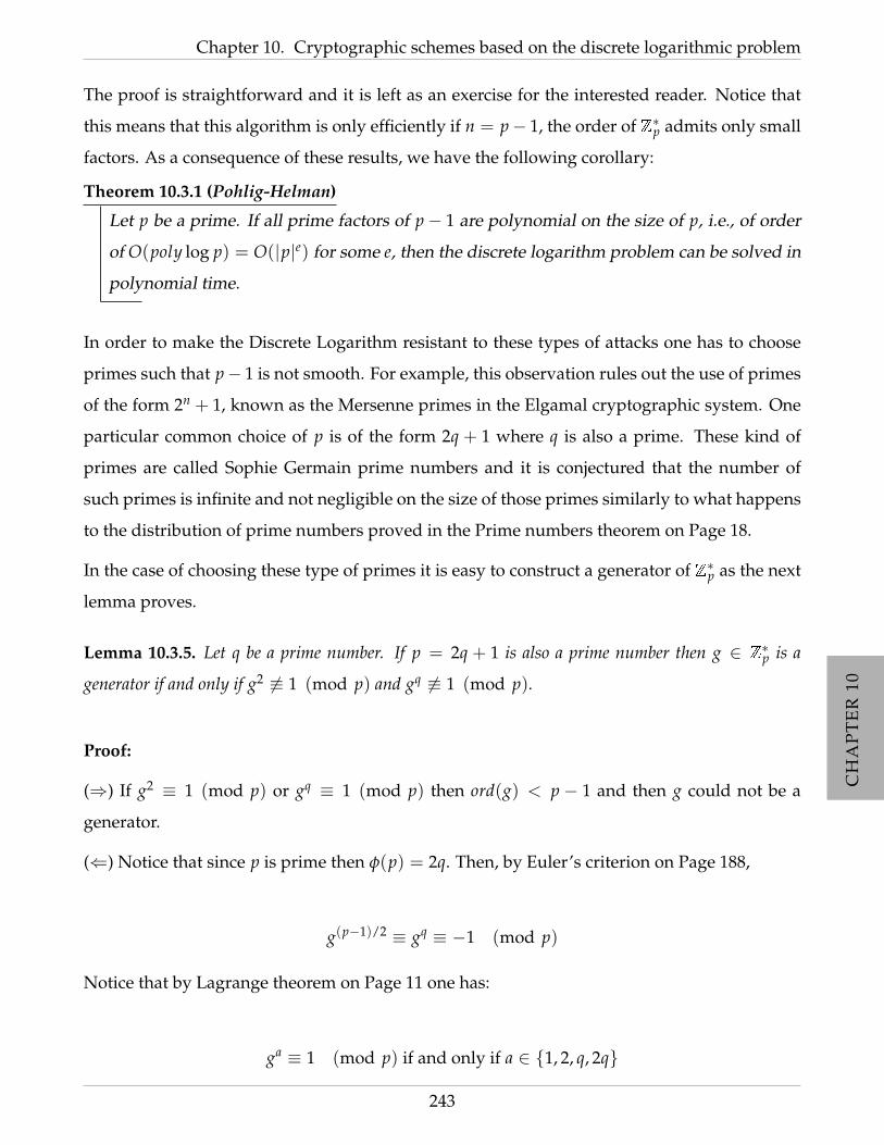
CH

AP

TE

R10

CH

AP

TE

R10

CH

AP

TE

R10

CH

AP

TE

R10

CH

AP

TE

R10

CH

AP

TE

R10

CH

AP

TE

R10

CH

AP

TE

R10

CH

AP

TE

R10


The proof is straightforward and it is left as an exercise for the interested reader. Notice that

this means that this algorithm is only efficiently if n = p− 1, the order of Z∗p admits only small

factors. As a consequence of these results, we have the following corollary:

Theorem 10.3.1 (Pohlig-Helman)

Let p be a prime. If all prime factors of p− 1 are polynomial on the size of p, i.e., of order

of O(poly log p) = O(|p|e) for some e, then the discrete logarithm problem can be solved in

polynomial time.

In order to make the Discrete Logarithm resistant to these types of attacks one has to choose

primes such that p− 1 is not smooth. For example, this observation rules out the use of primes

of the form 2n + 1, known as the Mersenne primes in the Elgamal cryptographic system. One

particular common choice of p is of the form 2q + 1 where q is also a prime. These kind of

primes are called Sophie Germain prime numbers and it is conjectured that the number of

such primes is infinite and not negligible on the size of those primes similarly to what happens

to the distribution of prime numbers proved in the Prime numbers theorem on Page 18.

In the case of choosing these type of primes it is easy to construct a generator of Z∗p as the next

lemma proves.

Lemma 10.3.5. Let q be a prime number. If p = 2q + 1 is also a prime number then g ∈ Z∗p is a

generator if and only if g2 6≡ 1 (mod p) and gq 6≡ 1 (mod p).

Proof:

(⇒) If g2 ≡ 1 (mod p) or gq ≡ 1 (mod p) then ord(g) < p − 1 and then g could not be a

generator.

(⇐) Notice that since p is prime then φ(p) = 2q. Then, by Euler’s criterion on Page 188,

g(p−1)/2 ≡ gq ≡ −1 (mod p)

Notice that by Lagrange theorem on Page 11 one has:

ga ≡ 1 (mod p) if and only if a ∈ 1, 2, q, 2q

243

CH

AP

TE

R10

CH

AP

TE

R10

CH

AP

TE

R10

CH

AP

TE

R10

CH

AP

TE

R10

CH

AP

TE

R10

CH

AP

TE

R10

CH

AP

TE

R10

CH

AP

TE

R10


So a as to be equal to 2q. Notice that since g2 6≡ 1 (mod p) then a cannot be 2 and thus it also

cannot be one. Also sincegq 6≡ 1 (mod p) then the only case left is a = 2q.

As a corollary one has:

Corollary 10.3.6. Let q be a prime number. If p = 2q + 1 is also a prime number and g ∈ Z∗p is a

generator and for odd i, q 6 |i then gi is also a generator.

Notice that by Fermat’s little theorem presented in Page 22, one has:

(g2i)q ≡ 1 (mod p)

and

(gq)2 ≡ 1 (mod p)

Then among the 2q elements of Z∗p, q + 1 are not generators of the group. So the following

algorithm can determine a generator of Z∗p.

Algorithm 10.3.7

Input a group Z∗p with p prime of the form p = 2q + 1 where q is another prime.

Output a generator of Z∗p.

Step 1 Choose uniformly at random g ∈ Z∗p;

Step 2 If g2 ≡ 1 (mod p) and gq 6≡ 1 (mod p) then output g else go to Step 1;

Notice that the probability of the algorithm has to repeat k times is roughly 1/2k and thus, on

average, this algorithm will find a generator after a small number of steps.

Another way of attacking the Discrete Logarithm is similar to attacks of the RSA cryptographic

system. In the sequel it is discussed a problem that is equivalent to the Discrete Logarithm

problem, namely the computation of the second least significant bit. Formally, consider the

following problem:

244

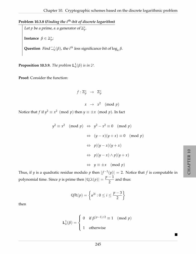
CH

AP

TE

R10

CH

AP

TE

R10

CH

AP

TE

R10

CH

AP

TE

R10

CH

AP

TE

R10

CH

AP

TE

R10

CH

AP

TE

R10

CH

AP

TE

R10

CH

AP

TE

R10


Problem 10.3.8 (Finding the ith-bit of discrete logarithm)

Let p be a prime, α a generator of Z∗p.

Instance β ∈ Z∗p;

Question Find Liα(β), the ith less significance bit of logα β.

Proposition 10.3.9. The problem L1α(β) is in P.

Proof: Consider the function:

f : Z∗p → Z∗p

x → x2 (mod p)

Notice that f if y2 ≡ x2 (mod p) then y ≡ ±x (mod p). In fact

y2 ≡ x2 (mod p) ⇔ y2 − x2 ≡ 0 (mod p)

⇔ (y− x)(y + x) ≡ 0 (mod p)

⇔ p|(y− x)(y + x)

⇔ p|(y− x) ∧ p|(y + x)

⇔ y ≡ ±x (mod p)

Thus, if y is a quadratic residue modulo p then | f−1(y)| = 2. Notice that f is computable in

polynomial time. Since p is prime then |QR(p)| = p− 12

and thus:

QR(p) =

α2i : 0 ≤ i ≤ p− 32

then

L1α(β) =

0 if β(p−1)/2 ≡ 1 (mod p)

1 otherwise

245

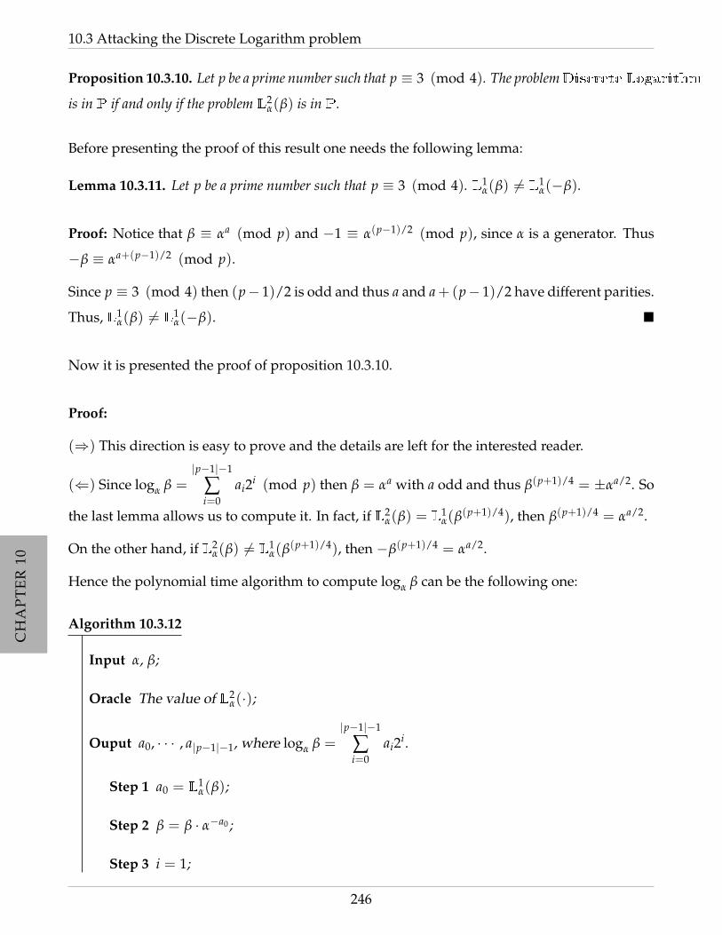
CH

AP

TE

R10

CH

AP

TE

R10

CH

AP

TE

R10

CH

AP

TE

R10

CH

AP

TE

R10

CH

AP

TE

R10

CH

AP

TE

R10

CH

AP

TE

R10

CH

AP

TE

R10


Proposition 10.3.10. Let p be a prime number such that p ≡ 3 (mod 4). The problemDiscrete Logarithm

is in P if and only if the problem L2α(β) is in P.

Before presenting the proof of this result one needs the following lemma:

Lemma 10.3.11. Let p be a prime number such that p ≡ 3 (mod 4). L1α(β) 6= L1

α(−β).

Proof: Notice that β ≡ αa (mod p) and −1 ≡ α(p−1)/2 (mod p), since α is a generator. Thus

−β ≡ αa+(p−1)/2 (mod p).

Since p ≡ 3 (mod 4) then (p− 1)/2 is odd and thus a and a+(p− 1)/2 have different parities.

Thus, L1α(β) 6= L1

α(−β).

Now it is presented the proof of proposition 10.3.10.

Proof:

(⇒) This direction is easy to prove and the details are left for the interested reader.

(⇐) Since logα β =|p−1|−1

∑i=0

ai2i (mod p) then β = αa with a odd and thus β(p+1)/4 = ±αa/2. So

the last lemma allows us to compute it. In fact, if L2α(β) = L1

α(β(p+1)/4), then β(p+1)/4 = αa/2.

On the other hand, if L2α(β) 6= L1

α(β(p+1)/4), then −β(p+1)/4 = αa/2.

Hence the polynomial time algorithm to compute logα β can be the following one:

Algorithm 10.3.12

Input α, β;

Oracle The value of L2α(·);

Ouput a0, · · · , a|p−1|−1, where logα β =|p−1|−1

∑i=0

ai2i.

Step 1 a0 = L1α(β);

Step 2 β = β · α−a0 ;

Step 3 i = 1;

246

CH

AP

TE

R10

CH

AP

TE

R10

CH

AP

TE

R10

CH

AP

TE

R10

CH

AP

TE

R10

CH

AP

TE

R10

CH

AP

TE

R10

CH

AP

TE

R10

CH

AP

TE

R10


Step 4 While (β 6= 1) do :

Step 4.1 ai = L2α(β);

Step 4.2 β = β(p+1)/4 (mod p);

Step 4.3 If ai 6= L1α(β) then β = −β (mod p);

Step 4.4 β = βα−ai ;

Step 4.5 i = i + 1;

Step 5 Output a0, · · · , a|p−1|−1;

• • • • • • • • • • • • • • • • • • • • • • • • • • • • • • • • • • • • •

SECTION 10.4

The elliptic curves

The use of elliptic curve in the public key cryptography was proposed independently by Neal

Koblitz and Victor S. Miller in the middle of 80’s and explores the algebraic properties and

structure of elliptic curves over finite fields to design public key cryptographic systems that are

believed to be secure, at least in computational term, i.e., secure in practice. These structures

are also used in several integer factorization algorithms that have applications in cryptography,

such as, for instance, Lenstra elliptic curve factorization, but this use of elliptic curves is ”not”

usually referred to as ”elliptic curve cryptography.”

Informally, an elliptic curve over the real plane is a set of points (x, y) that are solutions of the

equations of the form y2 = x3 + ax + b. These equations, known as Weierstrass equations, can

also be realized as a zero of a cubic function of two variables f (x, y) = y2− x3− ax− b and for

that reason they are sometimes also called cubic curves.

As it will be since in this section, the restriction of having elliptic curves over R2 is merely

artificial and used for sake of readability and understanding. In fact, ti will be considered

elliptic curves over finite fields in general.

247

CH

AP

TE

R10

CH

AP

TE

R10

CH

AP

TE

R10

CH

AP

TE

R10

CH

AP

TE

R10

CH

AP

TE

R10

CH

AP

TE

R10

CH

AP

TE

R10

CH

AP

TE

R10

10.4 The elliptic curves

The basic idea behind the use of these curves is the fact that one can form an abelian group with

the set of points on such curve together with a special point, called a point at infinity which

plays the role of the identity element of the group. Thus, if one choses (x, y) in a large finite

field, the solutions form a finite abelian group and thus it is possible to used similar techniques

too the ones used in the previous Section.

The resilience of elliptic curve based protocols against attacks is based on the hardness of

discrete logarithm over a random elliptic curve elements with respect to a publicly known base

point. The size of the elliptic curve determines the difficulty of the problem as it determines the

base where the logarithm is performed. For the moment, the greatest advantage of the use of

these structures when compared with their counterparts in Zp is that they seem to be harder to

break. Thus the keys keys for the protocols based on elliptic curve can be much smaller when

compared with the cases of the last Section, to achieve a similar level of security confidence. It

is also worthwhile mentioning that all this security is virtual in the sense, that similar to what

happens with RSA foundations, the problem that elliptic curves rely on is not to know to be

feasible. If one find a polynomial time algorithm to compute the discrete logarithm then all

these theory can not be used in practice as a secure encryption scheme. Despite this fact, and

like RSA, the U.S. National Security Agency has endorsed the cryptographic system based on

elliptic curves as one of the recommended algorithms that everyone should use.

Due to its relevance that they will play in this section, it is worthwhile emphasizing the def-

inition of an elliptic curve. Here it is already presented the most general definition of it. In

particular one can define an elliptic curve over any finite field in a similar way that one would

do over the field of real numbers.

Definition 10.4.1

Let F a field and let a, b two elements of F. An elliptic curve E over over F[x, y] is defined

as the following set:

E = (x, y) ∈ F×F : y2 − x3 − ax + b = 0.

In the next figure it is presented the most common curves that one can use when F is the set of

real numbers with classical operations.

248

CH

AP

TE

R10

CH

AP

TE

R10

CH

AP

TE

R10

CH

AP

TE

R10

CH

AP

TE

R10

CH

AP

TE

R10

CH

AP

TE

R10

CH

AP

TE

R10

CH

AP

TE

R10


a = -2

a = 1

a = -1

a = 0

b = -1 b = 0 b = 1 b = 2

Figure 10.1: Examples of some Elliptic curves

The particular interest of this curves is when they are non-singlular, i.e., when they have three

three distinct solutions which is equivalent to impose the condition that the partial derivatives

do not vanish simultaneously for any point of the curve simultaneously. It can be shown, and

is left to the interested reader to prove that the following condition is sufficient to guarantee

the non-sigularity of the curve:

249

CH

AP

TE

R10

CH

AP

TE

R10

CH

AP

TE

R10

CH

AP

TE

R10

CH

AP

TE

R10

CH

AP

TE

R10

CH

AP

TE

R10

CH

AP

TE

R10

CH

AP

TE

R10


Theorem 10.4.1

Let K a field and E an elliptic curve over K[x, y], i.e., E is the set of solution of the function

f (x, y) = 0 where f (x, y) = y2 − x3 − ax + b.

E is non singular if and only if 4a3 + 27b2 is not zero in F.

Usually the field that are used to consider in cryptography based on elliptic curves are of two

special types: fields of odd characteristic i.e., Fp, where p > 3 is a large prime number and

fields of characteristic two, i.e., of the form F2m . In the former case one uses simple modular

algebra and in the latter one, also known as Galois fields, one uses polynomials and operations

between them to represent the structure, that it will be explained in detail in due course. For

this case, and for technical reasons, the set E is defined as the pairs (x, y) such that y2 − xy−

x3 − ax + b = 0.

So, in order to use the this algebraic structures in cryptography it is necessary to define a binary

operation over E, normally denoted by addition, that enriches E to an abelian group. Now it is

explained how one can define the operations.

The addition of the point at infinity, which herein is denoted byO, plays the role of the identity

of the addition defined over the elliptic curve, i.e., for all P ∈ E

P +O = O + P = P

Now lets explain how the operation is determined.

Let P = (xP, yP) be a point in the elliptic curve E and define −P as the point with coordinates

(xP,−yP) if E is defined over Fp and define −P as the point with coordinates (xP, xP + yP) if E

is defined over F2m . Clearly, one has −P ∈ E for all P ∈ E.

Notice that if P and Q are two points on the curve E, then they uniquely determine a third

point, that will be defined as their sum, which is the intersection of the curve with the line

through P and Q. If that line is tangent to the curve at a point, then that point is counted

twice and if the line is parallel to the y-axis, the third point is defined as the point ”at infinity”.

Exactly one of these conditions then holds for any pair of points on an elliptic curve.

250

CH

AP

TE

R10

CH

AP

TE

R10

CH

AP

TE

R10

CH

AP

TE

R10

CH

AP

TE

R10

CH

AP

TE

R10

CH

AP

TE

R10

CH

AP

TE

R10

CH

AP

TE

R10


P

P

R

Q

Q

P

P

Q

1 2 3 4

P + Q + R = 0 P + Q + Q = 0 P + Q + 0 = 0 P + P + 0 = 0

Figure 10.2: Some examples of how to define p + q in an elliptic curve

Thus the operation + over E can be defined more concretely as follows:

• if Q = O then P + Q = P;

• if Q = −P then P + Q = O;

• if Q 6= P then define P + Q to be the point R = (xR, yR) where in the case E is defined

using Fp, xR = λ2 − xP − xQ, yR = λ(xP − xR) − yP, and λ =yQ − yP

xQ − xP. On the other

hand, if E is defined using F2m , xR = λ2 + λ + xP + xQ + a, yR = λ(xP + xR) + xR + yP,

and λ =yP + yQ

xP + xQ.1

• if Q = P then define P + Q to be the point R = (xR, yR) where in the case E is defined

using Fp, xR = λ2 − 2xP, yR = λ(xP − xR)− yP, and λ =3x2

P + a2yP

. On the other hand, if

E is defined using F2m , xR = λ2 + λ + a, yR = x2P + (λ + 1)xR, and λ = xP +

yP

xP.2

It is straightforward to prove E together with this binary operation is a group. Moreover, one

can use Hasse’s theorem on elliptic curves to estimate the number point on the elliptic curve.

1Geometrically, P + Q is the inverse over the axis x of the third point of intersection of the cubic with the line

through P and Q.2Geometrically, 2P is the inverse of the third point of intersection of the cubic with its tangent line at P.

251

CH

AP

TE

R10

CH

AP

TE

R10

CH

AP

TE

R10

CH

AP

TE

R10

CH

AP

TE

R10

CH

AP

TE

R10

CH

AP

TE

R10

CH

AP

TE

R10

CH

AP

TE

R10


The theorem states this result showing that that number is close to the size of the underlying

field. More precisely:

Theorem 10.4.2 (Hasse theorem)

Let E be an elliptic curve over a field of the form Fq where q > 3 is a prime number or

q = 2m for some m. Then

(√

q− 1)2 ≤ #E ≤ (√

q + 1)2

The exact computation of the cardinality of E can be done in polynomial time, due to Schoof,

which runs in is O((log p)8). Thus, if one can use further properties of this group, namely

a cyclic subgroup in which the Discrete Logarithm problem is intractable then one can im-

plement a generalized ElGamal cryptographic system in the elliptic curves. The following

theorem gives the idea one can do that.

Theorem 10.4.3

Let E be an elliptic curve defined over Fq where q > 3 is a prime number. Then there exist

positive integers n1 and n2 such that (E,+) is isomorphic to Zn1 × Zn2 . Furthermore, n2|n1

and n2|(p− 1).

Clearly, one can have n2 = 1, which happens if and only if E is a cyclic group. Also, if #E is

a prime, or product of distinct primes, then E must be a cyclic group. In all the other cases

one knows by the previous theorem if the integers n1 and n2 are computed, then one can

compute the cyclic subgroup that can potentially be used to define an ElGamal generalized


Notice that one can apply generic algorithms to the elliptic curve Discrete Logarithm problem.

However, one can explore an explicit isomorphism between elliptic curves and finite fields

that leads to efficient algorithms for certain classes of elliptic curves. This technique, due to

Menezes, Okamoto and Vanstone, can be applied to some particular examples within a special

class of elliptic curves called super singular curves that were suggested for use in cryptographic

systems.

On the other hand one can define another kind of cryptographic system based on elliptic curves

other than the generalized ElGamal cryptographic system. That scheme is presented now:

252

CH

AP

TE

R10

CH

AP

TE

R10

CH

AP

TE

R10

CH

AP

TE

R10

CH

AP

TE

R10

CH

AP

TE

R10

CH

AP

TE

R10

CH

AP

TE

R10

CH

AP

TE

R10


Cryptographic system 10.4.1 (Menezes - Vanstone Cryptographic system)

Consider p a prime number, E as the elliptic curve underlined by Z∗p and H a cyclic sub-

group of E. The Menezes - Vanstone Cryptographic system is the tuple EV = (P, C, K, E, D, R, r)

where:

1. P = Z∗p ×Z∗p;

2. C = E×Z∗p ×Z∗p;

3. K consists of tuples k = (α, a, β) such that β = aα in E and α is a generator of H;

4. R = E2;

5. Given a tuple (α, a, β), r(α, a, β) = (α, β);

6. For each k = (α, a, β) ∈ K and all x = (x1, x2) ∈ P, er(k)(x) = (y1, y2, y3) where

y1 = cα, where c ∈ Z is chosen at random and y2 = c1x1 (mod p) and y3 = c2x2

(mod p) where (c1, c2) = cβ.

7. d(α,a,β)(y1, y2, y3) = (x1, x2) where x1 = y2c−11 (mod p) and x2 = y2c−1

2 (mod p),

where (c1, c2) = ay1.

253

CH

AP

TE

R10

CH

AP

TE

R10

CH

AP

TE

R10

CH

AP

TE

R10

CH

AP

TE

R10

CH

AP

TE

R10

CH

AP

TE

R10

CH

AP

TE

R10

CH

AP

TE

R10


254

CH

AP

TE

R11

CH

AP

TE

R11

CH

AP

TE

R11

CH

AP

TE

R11

CH

AP

TE

R11

CH

AP

TE

R11

CH

AP

TE

R11

CH

AP

TE

R11

CH

AP

TE

R11

CH

AP

TE

R11

CHAPTER 11

Another approach to factorization -

Shor’s quantum algorithms

In last couple of chapters, it was discussed cryptography based of presumably hard problems

such as factoring composite numbers and the discrete logarithm problem and all the security

that every cryptography relies on is the fact that no one have ever came with an efficient

algorithm to solve these problems. But since the advent of quantum computing this apparent

idea of security it is dangerous as it is similar to be walking on thin ice. In fact, the apparent idea

of ??security is so misleading that since the advent of quantum computation it is known that

cryptography as described before, i.e., based on the hardness of factoring composite numbers

and the discrete logarithm is no longer possible as it had been proved that with a mechanism

that is capable of dealing with quantum information at hand, one can factor number and de-

termine the discrete logarithm among other apparently hard problems for classical computers

very efficiently.

Hence, in this chapter it is discussed a very different approach to cryptology, i.e., the science of

code breaking. It is based on the quantum computation, a conceptually different paradigm of

computation that is governed by the rules of the quantum mechanics.

There are several reasons to justify the study of quantum computation. In particular, several

experiments had showed that one can, in fact, implement a quantum mechanics models to

255

CH

AP

TE

R11

CH

AP

TE

R11

CH

AP

TE

R11

CH

AP

TE

R11

CH

AP

TE

R11

CH

AP

TE

R11

CH

AP

TE

R11

CH

AP

TE

R11

CH

AP

TE

R11

CH

AP

TE

R11

capture accurately real physical systems and the interactions between them. Furthermore these

experiments show that this model is more efficient than classical model of Turing machines in

the sense that are problems provably exponentially more efficiently solvable in a quantum com-

puting model than in a classical one; It is also robust, since one can perform error correction, to

make implementations robust to noise. This is an essential feature for implementability, which

several analog computing models cannot achieve.

Bits, or “binary digits” lie at the heart of all modern digital equipment and nowadays com-

puters use voltage levels to encode bits. All digital devices deal with them and one can use

their properties without even noticing them. One can read a bit to learn its value, one can copy,

erase or negate it; and one can read some of the bits inside a digital device without changing

the other bits that one did not read. In fact such properties seem so obvious that no one even

bothers to question these assumptions. However, Richard Feynman anticipated that very small

physical devices would be governed by quantum mechanics rather than classical mechanics

and, accordingly, would not necessarily behave similarly as their larger counterparts. At the

subatomic level a bit can be 0 or 1 at the same time and if one wishes to know, for sure its

value, one has to perform an observation. This interaction with the system makes a permanent

record of the result and hence its behavior becomes definite. That sounds crazy, but that is

what quantum mechanics tells that actually happen.

As devices become smaller and smaller the physical systems used to encode those bits will

become smaller and their behavior will need to be described using quantum mechanics.

At this level the common sense assumptions about how bits ought to behave (read, copy, erase,

negate them without causing them to change in any way) might not be true anymore. In fact,

at the quantum level one cannot necessarily read a bit without changing its value; one cannot

copy, or negate it without perturbing it; one may be unable to erase it; and sometimes when

one reads the smallest piece of information, these actions can change the state to another with

which the reader had never interacted with. Thus, bits encoded in quantum-scale objects cease

to behave like normal bits ought.

Quantum computation and quantum information are built upon an analogous concept to bit,

which are known as quantum bit or shortly by qubit. The idea is that quantum computation

systems is one can encode information in a physical states of the system. For example, when

256

CH

AP

TE

R11

CH

AP

TE

R11

CH

AP

TE

R11

CH

AP

TE

R11

CH

AP

TE

R11

CH

AP

TE

R11

CH

AP

TE

R11

CH

AP

TE

R11

CH

AP

TE

R11

CH

AP

TE

R11

Chapter 11. Another approach to factorization - Shor’s quantum algorithms

the spin of a electron is measured it can be found in only two possible values, either “spin

up” (|↑〉) parallel to the axis or “spin down” (|↓〉) anti-parallel to the axis along which the

measurement was taken. This intrinsic discreteness, a manifestation of quantization, allows

the spin of an electron to be considered as a natural binary digit or “bit”. The resulting system

is the quantum bit.

• • • • • • • • • • • • • • • • • • • • • • • • • • • • • • • • • • • • •

SECTION 11.1

Notation

Now it is presented the classical notation used in the quantum computational field. The

information in quantum is quite different from the classical information. Rather than having

just two possible states for each unit of information, one can have a quantum bit into an infinite

range. In fact, the quantum bit exists in a superposition of two states. A quantum bit is usually

represented in Dirac notation as a “ket” of the form |φ〉 and in general one considers two

directions, more accurately spins, |0〉 or |1〉. Thus |ψ〉 is a linear combination of the form

α|0〉+ β|1〉, where α and β are complex numbers.

The possible infinite amount of information in a quantum bit has a drawback. One can not

observe them, i.e, the observation of a quantum bit is doable up to the penalty to collapse of

the superposition into one of the directions considered. Either |0〉 or |1〉.

This presents the first restriction that one must consider for each quantum bit. In fact, a

quantum bit is of the form |ψ〉 = α|0〉+ β|1〉 where α and β must satisfy |α|2 + |β|2 = 1.

Similarly to what happens in the classical information, the power of the quantum informa-

tion is given possibility of combining two or more basic information units. In the quantum

information theory, to combine several quantum bits, instead of simply concatenate, similar to

classical, we need to adopt the tensor product, represented by ⊗.

257

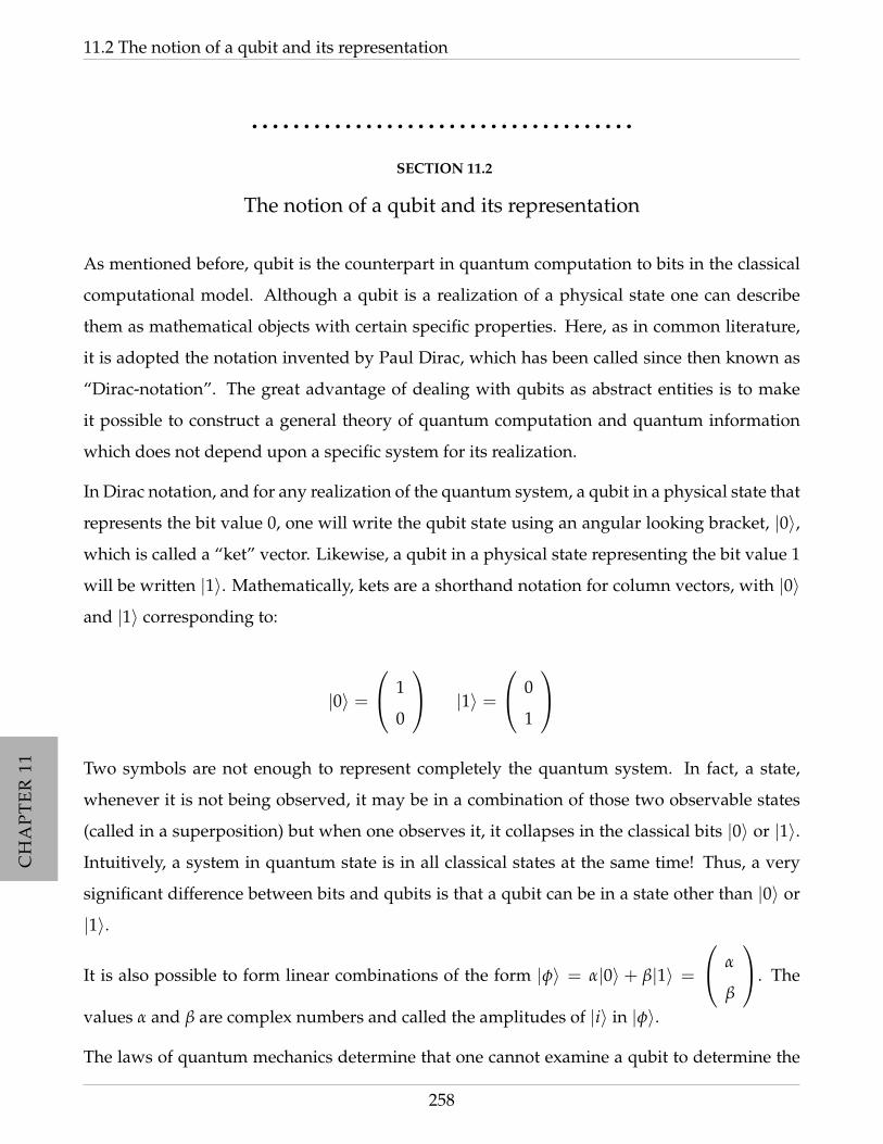
CH

AP

TE

R11

CH

AP

TE

R11

CH

AP

TE

R11

CH

AP

TE

R11

CH

AP

TE

R11

CH

AP

TE

R11

CH

AP

TE

R11

CH

AP

TE

R11

CH

AP

TE

R11

CH

AP

TE

R11

11.2 The notion of a qubit and its representation

• • • • • • • • • • • • • • • • • • • • • • • • • • • • • • • • • • • • •

SECTION 11.2

The notion of a qubit and its representation

As mentioned before, qubit is the counterpart in quantum computation to bits in the classical

computational model. Although a qubit is a realization of a physical state one can describe

them as mathematical objects with certain specific properties. Here, as in common literature,

it is adopted the notation invented by Paul Dirac, which has been called since then known as

“Dirac-notation”. The great advantage of dealing with qubits as abstract entities is to make

it possible to construct a general theory of quantum computation and quantum information

which does not depend upon a specific system for its realization.

In Dirac notation, and for any realization of the quantum system, a qubit in a physical state that

represents the bit value 0, one will write the qubit state using an angular looking bracket, |0〉,

which is called a “ket” vector. Likewise, a qubit in a physical state representing the bit value 1

will be written |1〉. Mathematically, kets are a shorthand notation for column vectors, with |0〉

and |1〉 corresponding to:

|0〉 =

1

0

|1〉 =

0

1

Two symbols are not enough to represent completely the quantum system. In fact, a state,

whenever it is not being observed, it may be in a combination of those two observable states

(called in a superposition) but when one observes it, it collapses in the classical bits |0〉 or |1〉.

Intuitively, a system in quantum state is in all classical states at the same time! Thus, a very

significant difference between bits and qubits is that a qubit can be in a state other than |0〉 or

|1〉.

It is also possible to form linear combinations of the form |φ〉 = α|0〉 + β|1〉 =

α

β

. The

values α and β are complex numbers and called the amplitudes of |i〉 in |φ〉.

The laws of quantum mechanics determine that one cannot examine a qubit to determine the

258

CH

AP

TE

R11

CH

AP

TE

R11

CH

AP

TE

R11

CH

AP

TE

R11

CH

AP

TE

R11

CH

AP

TE

R11

CH

AP

TE

R11

CH

AP

TE

R11

CH

AP

TE

R11

CH

AP

TE

R11


values of the amplitudes. Recall that once a measure is done, i.e., an observation is performed,

the quantum bit collapses in one of the classical states. Hence one is only able to acquire

much more restricted information about the quantum state using a proper normalization that

guarantees that these classical states are reached, 0 with probability |α|2, and 1 with probability

|β|2, and thus, the amplitudes satisfy |α|2 + |β|2 = 1.

Thus, a single qubit is an element of the vector space C2. In fact, geometrically, one can see a

qubit as an element of a sphere to radius 1 (known as the Bloch sphere). In general a qubit’s

state is a unit vector in a two-dimensional complex vector space.

One can use a similar idea to work with more than one qubit. They are formally represented

by a tensor product space of several qubit systems. For example, a 2-qubit system has 4 basis

states: |0〉 ⊗ |0〉, |0〉 ⊗ |1〉, |1〉 ⊗ |0〉 and |1〉 ⊗ |1〉 where the first element represents the sate of

the first qubit and the second element represents the state of the second qubit. For simplicity,

it is common to represent |0〉 ⊗ |0〉 by the following short notation |00〉.

More generally, a register of n qubits has 2n basis states, which is of the form |b1〉⊗ · · · ⊗ |b2n〉 =

|b1 · · · b2n〉. Since any bit string of length n can be viewed as numbers between 0 and 2n − 1,

one can also write the basis states as numbers |0〉, ...,∣∣2n−1⟩. A quantum register of n qubits

can be in any superposition

α0|0〉+ · · ·+ α2n−1|2n − 1〉

or

α0|0 · · · 0〉+ α1|0 · · · 01〉+ · · ·+ α2n−1|1 · · · 1〉

and the amplitudes αi satisfy2n−1

∑i=0|αi|2 = 1. If one performs a measure in the standard basis,

we obtain a n-bit state, and in particular one gets the state |j〉 with probability |αj|2.

Here we analyze how quantum computation is performed and the kind of operations we can

apply in quantum information.

It is known and it will be discussed later in this chapter, that quantum computation must obey

some rules in order to be consistent. Notice that, for example, a quantum qubit α|0〉 + β|1〉

must satisfy that |α|2 + |β|2 = 1. It can be seen in several ways, but remember, for example

the Bloch sphere, where all vectors are expected to have norm 1. Thus, when one applies

259

CH

AP

TE

R11

CH

AP

TE

R11

CH

AP

TE

R11

CH

AP

TE

R11

CH

AP

TE

R11

CH

AP

TE

R11

CH

AP

TE

R11

CH

AP

TE

R11

CH

AP

TE

R11

CH

AP

TE

R11


a quantum operation to a qubit, at the end of the evolution, and in fact in between, one

expects that the resulting quantum bit satisfies the same rule. This give the main criteria to

the kind of operations one must deal with in quantum computation. Indeed, any quantum

transformation must be unitary. Consequently all quantum transformations preserve inner

products and hence also norms.

It is now surveyed the most used quantum operations by presenting several examples of

quantum circuits and explain their effect on quantum states.

Now it is paid attention to the description of how one can use quantum model of representing

information to do computations, i.e., changes to the quantum states, by describing how qubits

can evolve within a qauntum system. There are several approaches to describe the evolution

of the system that all equivalent.

As discussed in the introduction of this chapter all transformation that one can apply to a

quantum register must be unitary. The formal definition of this notion is as follows:

Definition 11.2.1

Suppose A is any linear operator on a Hilbert space, V.

Then, there exists unique linear operator A† on V such that for all vectors v, w ∈ V,

〈v|Aw〉 =⟨

A†v|w⟩

This linear operator is known as the adjoint or Hermitian conjugate of the operator A. From

the definition it is easy to see that (AB)† = B† A†.

If the operator A is represented by a matrix, the action of the Hermitian conjugation oper-

ation corresponds to take the matrix of A to the conjugate-transpose matrix, A† = (A∗)T,

where the ∗ indicates complex conjugation, and T indicates the transpose operation.

A transformation A such that A(A)† = I is called unitary.

Example : Let A be the operator described by the matriz

A =

1 + i 2i

1 4− i

260

CH

AP

TE

R11

CH

AP

TE

R11

CH

AP

TE

R11

CH

AP

TE

R11

CH

AP

TE

R11

CH

AP

TE

R11

CH

AP

TE

R11

CH

AP

TE

R11

CH

AP

TE

R11

CH

AP

TE

R11


Then its adjoint is:

A† =

1 + i 2i

1 4− i

∗T

=

1− i −2i

1 4 + i

T

=

1− i 1

−2i 4 + i

An operator A whose adjoint is itself, i.e., A† = A is called a Hermitian or self-adjoint operator.

An important example of Hermitian operators is the projectors. If W is a subspace of dimension

k of V (of dimension d > k) then the projection defined of V on W is defined by

P = ∑i=1

k|i〉〈i|

where we assume that the base of V is |1〉, · · · |d〉.

An operator A is normal if AA† = A† A. Clearly, an operator which is Hermitian is also normal.

Theorem 11.2.1

A normal matrix is Hermitian if and only if it has real eigenvalues.

A matrix U is unitary if U†U = UU† = I, i.e., U−1 = U†. It is easily checked that an operator is

unitary if and only if each of its matrix representations is unitary. A unitary operator is normal

and has a spectral decomposition. Geometrically, unitary operators are important because they

preserve inner products between vectors.

The reader showed check these equivalences to start to familiarize with these concepts.

• • •

11.2.1 Scoot Aaronson explains the Shor’s algorithm

Before presenting the algorithm, in this subsection, it is very interesting to present the discus-

sion about Shor’s algorithm in Scott Aaronson’s blog [?]. The description that he pulled out

is very simple and clear about this quantum algorithm and what it is all about. He is a very

smart guy and is specially gifted to put complex things into a very understandable way.

After this discussion, it presented the ground concepts need to understand the Shor’s algo-

rithm. Namely, it will discuss the quantum Fourier transformation, the quantum algorithm of

period finding (the kernel of speed up when compared with the classical counterpart) and then

the algorithm itself. An example that illustrates the algorithm is also given.

261

CH

AP

TE

R11

CH

AP

TE

R11

CH

AP

TE

R11

CH

AP

TE

R11

CH

AP

TE

R11

CH

AP

TE

R11

CH

AP

TE

R11

CH

AP

TE

R11

CH

AP

TE

R11

CH

AP

TE

R11


The importance of this algorithm is mainly due to the security code used in almost

every place we look at, the RSA code. Breaking RSA is just a matter of finding the

prime factors of a large integer N. If we try to do it classically it requires exponential

resources. The idea is to use the quantum phenomena to design a fast quantum

factoring algorithm and it is necessary to exploit some structure in the factoring

problem.

The properties that are important to explore in the factoring problem is the unique-

ness on the factorization itself and the reducibility of factoring to another problem,

called period-finding. Consider the sequence of powers of two:

2, 4, 8, 16, 32, 64, 128, 256, 512, 1024, · · ·

and consider them “ mod 15”: 2, 4, 8, 1, 2, 4, 8, 1, 2, 4, · · · .

Taking the powers of 2 mod 15 gives us a periodic sequence, whose period is 4.

This a general property and is a beautiful pattern discovered by Euler in the 1760’s:

Let N be a product of two prime numbers, p and q, and consider the sequence x

mod N, x2 mod N, x3 mod N, x4 mod N, · · · . If x is not divisible by p or q, the

sequence will repeat with some period that evenly divides (p− 1)(q− 1).

So for example, if N = 15, then the prime factors of N are p = 3 and q = 5, so

(p− 1)(q− 1) = 8. And indeed, the period of the sequence was 4, which divides 8.

So, this means that if we can find the period of the sequence x mod N, x2 mod N,

x3 mod N, x4 mod N... then we can learn something about the prime factors of

N! Indeed we can get a divisor of (p− 1)(q− 1). Indeed, it’s more than something:

it turns out that if we could learn several random divisors of (p − 1)(q − 1) (for

example, by trying different random values of x), then with high probability we

could put those divisors together to learn (p− 1)(q− 1) itself. And once we knew

(p − 1)(q − 1), we could then use some more little tricks to recover p and q, the

prime factors we wanted. In fact if r is the period can be shown that with probability

≥ 1/4, r is even and xr/2 + 1 and xr/2 − 1 are not multiples of N and then xr − 1 ≡

xr/2− 1 ≡ (xr/2 + 1)(xr/2− 1) ≡ 0, and thus xr/2 + 1 or xr/2− 1 will share a proper

factor with N. (So we get it using the Euclides’ algorithm for the great common

262

CH

AP

TE

R11

CH

AP

TE

R11

CH

AP

TE

R11

CH

AP

TE

R11

CH

AP

TE

R11

CH

AP

TE

R11

CH

AP

TE

R11

CH

AP

TE

R11

CH

AP

TE

R11

CH

AP

TE

R11


divisor). This is why finding the period does not seem to lead to a fast classical

factoring algorithm.

But we have a quantum computer! The key point is that we are no longer trying

to find a needle in an exponentially-large haystack, something we know is hard

even for a quantum computer. Instead, we are now trying to find the period of

a sequence, which is a global property of all the numbers in the sequence taken

together. And that makes a big difference.

If we want to get this period-finding idea to work, we’ll have to answer two ques-

tions:

1. Using a quantum computer, can we quickly create a superposition over x mod N,

x2 mod N, x3 mod N, and so on?

2. Supposing we did create such a superposition, how would we figure out the

period?

It is easy to create a superposition over all integers r, from 1 up to N or so. To

produce xr mod N we can do repeated squaring. If N = 17, x = 3 and r = 14.

Then the first step is to represent r as a sum of powers of 2: r = 23 + 22 + 21. Then

xr = 314 = 323+22+21= 323

+ 322321

= ((32)2)2(32)232.

Another advantage is to do all the multiplications mod N, thereby preventing the

numbers from growing out of hand at intermediate steps.

So given a superposition over all the elements of a periodic sequence, how do we

extract the period of the sequence?

Finally we come to the heart of the matter - the part of the algorithm that actually

depends on quantum mechanics. To get the period, Shor used the quantum Fourier

transform, or QFT.

To explain it consider the famous experiment where they stick people for weeks in

a sealed room without clocks or sunlight, and the people gradually shift from a 24-

hour day to a 25- or 26- or 28-hour day? One day, you wake up at 9am, the next day

263

CH

AP

TE

R11

CH

AP

TE

R11

CH

AP

TE

R11

CH

AP

TE

R11

CH

AP

TE

R11

CH

AP

TE

R11

CH

AP

TE

R11

CH

AP

TE

R11

CH

AP

TE

R11

CH

AP

TE

R11


at 11am, the day after that at 1pm, etc. Lets say I tell you that I woke up at 5pm this

afternoon. From that fact alone, what can you conclude about how long my “day”

is?

The answer, of course, is not much! Now, though, I want you to imagine that the

bedroom wall is covered with strange clocks: one of them makes a full revolution

every 17 hours, one of them every 26 hours, one of them every 24.7 hours, and so on

for just about every number of hours you can imagine and beneath each clock is a

posterboard with a thumbtack in it. When you first moved into the bedroom, each

thumbtack was in the middle of its respective board. But now, whenever you wake

up in the “morning” the first thing you do is to go around the room, and move each

thumbtack exactly one inch in the direction that the clock hand above it is pointing.

Now, the new question: by examining the thumbtacks in the room, is it possible to

figure out what sort of schedule you’re keeping?

The answer is Yes. As an example, suppose you keep a 26-hour day. Then what

would happen to the thumbtack below the 24-hour clock? It is not hard to see that it

would undergo periodic motion: sure, it would drift around a bit, but after every 12

days it would return to the middle of the board where it had started. One morning

you had move the thumbtack an inch in this direction, another morning an inch in

that, but eventually all these movements in different directions would cancel each

other out.

On the other hand and “again supposing you were keeping a 26-hour day” what

would happen to the thumback below the 26-hour clock? Here the answer is dif-

ferent. For as far as the 26-hour clock is concerned, you have been waking up at

exactly the same time each “morning” Every time you wake up, the 26-hour clock

is pointing the same direction as it was the last time you woke up. So I’ll keep

moving the thumbtack one more inch in the same direction, until it’s not even on

the posterboard at all!

It follows, then, that just by seeing which thumbtack traveled the farthest from its

starting point, you could figure out what sort of schedule you were on. And that,

basically, is the quantum Fourier transform.

264

CH

AP

TE

R11

CH

AP

TE

R11

CH

AP

TE

R11

CH

AP

TE

R11

CH

AP

TE

R11

CH

AP

TE

R11

CH

AP

TE

R11

CH

AP

TE

R11

CH

AP

TE

R11

CH

AP

TE

R11


A little more precisely, the QFT is a unitary transformation that maps one vector

of complex numbers to another vector of complex numbers. The input vector has

a nonzero entry corresponding to every time when you wake up, and zero entries

everywhere else. The output vector records the positions of the thumbtacks on the

posterboards (which one can think of as points on the complex plane). So what we

get, in the end, is a linear transformation that maps a quantum state encoding a

periodic sequence, to a quantum state encoding the period of that sequence.

Another way to think is in terms of interference. The key point about quantum me-

chanics - the thing that makes it different from classical probability theory - is that,

whereas probabilities are always nonnegative, amplitudes in quantum mechanics

can be positive, negative, or even complex. And because of this, the amplitudes

corresponding to different ways of getting a particular answer can “interfere de-

structively” and cancel each other out.

And that is exactly what is going on in Shor’s algorithm. Every “parallel universe”

corresponding to an element of the sequence contributes some amplitude to every

“parallel universe” corresponding to a possible period of the sequence. The catch

is that, for all periods other than the “true” one, these contributions point in dif-

ferent directions and therefore cancel each other out. Only for the “true” period

do the contributions from different universes all point in the same direction. And

that is why, when we measure at the end, we will find the true period with high

probability.

Scoot Aaronson

265

CH

AP

TE

R11

CH

AP

TE

R11

CH

AP

TE

R11

CH

AP

TE

R11

CH

AP

TE

R11

CH

AP

TE

R11

CH

AP

TE

R11

CH

AP

TE

R11

CH

AP

TE

R11

CH

AP

TE

R11


• • •

11.2.2 The Shor’s algorithm for factoring

Before presenting the algorithm it is needed some background on quantum Fourier transfor-

mations as these elements are crucial for the understanding of the result.

• • •

11.2.2.1 Quantum Fourier transformation

If computers that you build are quantum, then spies everywhere will all want ’em.

Our codes will all fail, and they’ll read our email. Till we get crypto that’s quantum, and

daunt ’em.

Jennifer and Peter Shor

The quantum Fourier transform is a linear transformation on quantum bits, and is the quan-

tum counterpart of the discrete Fourier transform and can be efficiently implemented using

O(n2) quantum gates (Hadamard and controlled phase shifts). The classical discrete Fourier

transform requires O(n2n) gates to be implemented. However, the quantum Fourier transform

acts on a quantum state, whereas the classical Fourier transform acts on a vector and it does

not speed up the classical task of computing Fourier transforms of classical data.

Classically the Fourier transform takes a vector of complex numbers, x0, · · · xN−1 where the

length N of the vector is a fixed parameter and outputs the transformed data, a vector of

complex numbers y1, · · · , yN−1 defined by

yk =1√N

N−1

∑j=0

xje2·π·i·j·k

N

The quantum Fourier transform is the quantum counterpart of this transformation. It is a linear

operator that on the basis states of an orthonormal basis |0〉 · · · |N − 1〉 operates by:

266

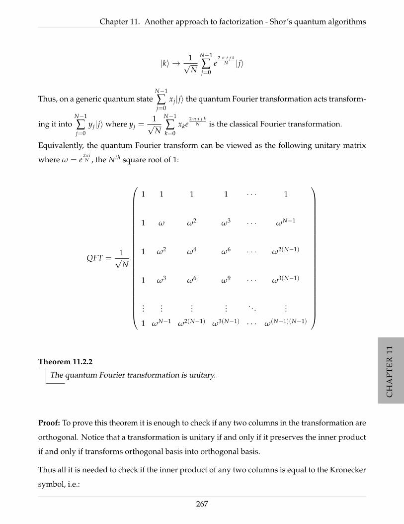
CH

AP

TE

R11

CH

AP

TE

R11

CH

AP

TE

R11

CH

AP

TE

R11

CH

AP

TE

R11

CH

AP

TE

R11

CH

AP

TE

R11

CH

AP

TE

R11

CH

AP

TE

R11

CH

AP

TE

R11


|k〉 → 1√N

N−1

∑j=0

e2·π·i·j·k

N |j〉

Thus, on a generic quantum stateN−1

∑j=0

xj|j〉 the quantum Fourier transformation acts transform-

ing it intoN−1

∑j=0

yj|j〉 where yj =1√N

N−1

∑k=0

xke2·π·i·j·k

N is the classical Fourier transformation.

Equivalently, the quantum Fourier transform can be viewed as the following unitary matrix

where ω = e2πiN , the Nth square root of 1:

QFT =1√N

1 1 1 1 · · · 1

1 ω ω2 ω3 · · · ωN−1

1 ω2 ω4 ω6 · · · ω2(N−1)

1 ω3 ω6 ω9 · · · ω3(N−1)

......

...... . . . ...

1 ωN−1 ω2(N−1) ω3(N−1) · · · ω(N−1)(N−1)

Theorem 11.2.2

The quantum Fourier transformation is unitary.

Proof: To prove this theorem it is enough to check if any two columns in the transformation are

orthogonal. Notice that a transformation is unitary if and only if it preserves the inner product

if and only if transforms orthogonal basis into orthogonal basis.

Thus all it is needed to check if the inner product of any two columns is equal to the Kronecker

symbol, i.e.:

267

CH

AP

TE

R11

CH

AP

TE

R11

CH

AP

TE

R11

CH

AP

TE

R11

CH

AP

TE

R11

CH

AP

TE

R11

CH

AP

TE

R11

CH

AP

TE

R11

CH

AP

TE

R11

CH

AP

TE

R11


〈i|QFT∗QFT|j〉 = δi,j =

1 if i = j

0 if i 6= j

Computing the inner product one has

〈i|QFT∗QFT|j〉 = 1N

N−1

∑k=0

ωi·kω j·k =1N

N−1

∑k=0

ωk(j−i)

which is a geometric series with ratio ω j−i. Thus if i = j mod N, then each term is equal to

ω0 = 1 and the inner product is then equal to N/N = 1.

If i 6= j, then the sum is

1 + ω j−i + ω2(j−i) + · · ·+ ω(N−2)(j−i) + ω(N−1)(j−i).

Notice that if we multiply the sum by ω j−i one gets,

ω j−i + ω2(j−i) + ω3(j−i) + · · ·+ ω(N−1)(j−i) + ωN(j−i).

But, since ω is a nth root of 1, ωN(j−i) = 1. Thus the multiplication it is just an rearrangement

of the sum and thus, since ω j−i 6= 0 one concludes that

1 + ω j−i + ω2(j−i) + · · ·+ ω(N−2)(j−i) + ω(N−1)(j−i) = 0.

The following circuit implements the quantum Fourier transformation:

268

CH

AP

TE

R11

CH

AP

TE

R11

CH

AP

TE

R11

CH

AP

TE

R11

CH

AP

TE

R11

CH

AP

TE

R11

CH

AP

TE

R11

CH

AP

TE

R11

CH

AP

TE

R11

CH

AP

TE

R11


|xn〉 • • · · · • · · · • H |y1〉

|xn−1〉

QFTn−1

· · · · · · Rπ/2 |y2〉

......

|xi〉 · · · Rπ/2n−i · · · |yn−i+1〉

......

|x2〉 Rπ/2n−2 · · · · · · |yn−1〉

|x1〉 Rπ/2n−1 · · · · · · |yn〉

The quantum Fourier transform can be approximately implemented for any N and in the

case where N = 2n one has a special representation of the quantum Fourier transformation

with respect to an orthonormal basis consisting of the vectors |0〉, · · · |2n − 1〉. Notice that

x = x12n−1 + x22n−2 + · · · xn20 can be represented by |x〉 = |x1 · · · xn〉 = |x1〉 · · · |xn〉. Also, if

x is a decimal number between 0 and 1 one can represent it using the decimal notation as

[0.x1 · · · xm] = ∑k=0

xk2−k.

Thus the quantum Fourier transform can be given by the following product representation:

|x1, x2, · · · , xn〉 →1√N(|0〉+ e2πi[0.xn]|1〉)⊗ (|0〉+ e2πi[0.xn−1xn]|1〉)⊗

⊗ · · · ⊗ (|0〉+ e2πi[0.x1···xn−1xn]|1〉)

This representation give the direction to construct an efficient quantum circuit computing the

Fourier transform, a proof that the quantum Fourier transform is unitary, and provides insight

into algorithms based upon the quantum Fourier transform.

269

CH

AP

TE

R11

CH

AP

TE

R11

CH

AP

TE

R11

CH

AP

TE

R11

CH

AP

TE

R11

CH

AP

TE

R11

CH

AP

TE

R11

CH

AP

TE

R11

CH

AP

TE

R11

CH

AP

TE

R11


• • •

11.2.2.2 The period finding

The problem of factoring numbers on a classical computer turns out to be equivalent to another

problem, the order-finding problem. This equivalence is important as it turns out that quantum

computers are able to quickly solve the order-finding problem, and thus can factor quicker than

one would do in a classical computer.

The order-finding problem is believed to be a hard problem classically, in the sense that, given

N an integer, no algorithm is known to solve it within polynomial resources, i.e., in O(log N)

steps.

Here it is described the procedure to find the period of a function. One is given a function f

and an integer N with the promise that there is a period, call it a ≤ N, such that for all x, y

one has f (x) = f (y) if and only if y ∈ x, xa, x2a, · · · . The period finding problem is just to

determine a.

Problem 11.2.1 (period finding)

Instance: A function f ;

Promise: f is periodic;

Question: Find the period of the function.

Algorithm 11.2.2 (Period finding)

Input: Let L be equal to log N. The inputs to the algorithm are:

1. A black box implementing the unitary transformation

Ux,N(|j〉|k〉) = |j〉∣∣∣xjk mod N

⟩where x is co-prime with N;

2. t = 2L + 1 +⌈

log(

2 +12e

)⌉qubits initialized to |0〉.

3. L qubits on the state |1〉.

270

CH

AP

TE

R11

CH

AP

TE

R11

CH

AP

TE

R11

CH

AP

TE

R11

CH

AP

TE

R11

CH

AP

TE

R11

CH

AP

TE

R11

CH

AP

TE

R11

CH

AP

TE

R11

CH

AP

TE

R11


Output: The least integer r > 0 such that xr ≡ 1( mod N).

Runtime: 0(L3) operations.

Success probability: 0(1).

Step 1 Apply the Quantum Fourier transformation to the first register of |0 · · · 0〉|1 · · · 1〉

to get:

1√2t

2t−1

∑j=0|j〉|1〉

Step 2 Apply Ux,N, and the result is:

1√2t

2t−1

∑j=0|j〉∣∣∣xj mod N

⟩Step 3 Measuring the second register we get a random |xs mod N〉 with s ≤ r and the

first register collapses to a superposition of |s〉, |s + r〉, |s + 2r〉, · · ·, |q− r + s〉, where

q =

⌊Nr

⌋(−1), (the −1 term is used in the case r|q).

Step 4 If r|q then the last state collapses into:

1√

q

q/r−1

∑j=0|jr + s〉

and one can apply a quantum Fourier transformation to obtain:

q/r−1

∑j=0

q−1

∑b=0

e2πi (jr+s)bq |b〉 =

q−1

∑b=0

e2πi sbq

(q/r−1

∑j=0

(e2πi sb

q)j)|b〉

Notice thatq/r−1

∑j=0

(e2πi sb

q)j

is a geometric sum. Notice that if a is the reason of the

geometric sum, then a0 + · · ·+ an =1− an+1

1− awhich is equal to q if sb/r is an integer

and 0 otherwise. Thus, in the first register, one only observes a state of the form b = c qr

with c < r and random.

271

CH

AP

TE

R11

CH

AP

TE

R11

CH

AP

TE

R11

CH

AP

TE

R11

CH

AP

TE

R11

CH

AP

TE

R11

CH

AP

TE

R11

CH

AP

TE

R11

CH

AP

TE

R11

CH

AP

TE

R11


b = cqr⇔ b

q=

cr

If c is co-prime with r (which happens with probability Ω(1/ log log r)) the algorithm

is done, since one knows b and q. In the case it is not known if c is co-primality,

running O(log log N) times this procedure one gets a factor of r and using the least

common multiplier one can recover r.

else i.e. r 6 |q, then one can not any longer writebq=

cr

but with very high probability

one observes b such that

∣∣∣∣bq − cr

∣∣∣∣ ≤ 12q

.

Since there is only one fraction with denominator < N in an interval of length1q≤ 1

N2

(see Theorem 11.2.3 below) one can computecr

using the continued fraction algorithm

(see Theorem 11.2.4).

Theorem 11.2.3

Let φ be a number between 0 and 1. If α/β is a rational number such that

∣∣∣∣αβ − φ

∣∣∣∣ ≤ 12β2

thenα

βis convergent of the continued fraction for φ and can be computed fast by th Euclid’s

algorithm.

Proof: TBW...

In the case considered, this is sufficient since it is known that φ up to a precision of 2L + 1 and

then it follows that

∣∣∣∣bq − cr

∣∣∣∣ ≤ 2−2L−1 ≤ 12r2

as r ≤ N ≤ 2L.

272

CH

AP

TE

R11

CH

AP

TE

R11

CH

AP

TE

R11

CH

AP

TE

R11

CH

AP

TE

R11

CH

AP

TE

R11

CH

AP

TE

R11

CH

AP

TE

R11

CH

AP

TE

R11

CH

AP

TE

R11


Theorem 11.2.4

Let x be any rational number. One can write x as

[a0, · · · , an] = a0 +1

a1 +1

a2 +1

1... +1M

.

Proof: TBW

Example 11.2.3.

1. The continued fraction of10013

is [7, 1, 2, 4]

10013

= 7 +9

13= 7 +

1139

= 7 +1

1 +49

= 7 +1

1 +194

= 7 +1

1 +1

2 +14

= [7, 1, 2, 4]

2. The continued fraction of3113

is [2, 2, 1, 1, 2]

3113

= 2 +5

13= 2 +

1135

= 2 +1

2 +35

= 2 +1

2 +153

= 2 +1

2 +1

1 +23

= 2 +1

2 +1

1 +132

= 2 +1

2 +1

1 +1

1 +12

= [2, 2, 1, 1, 2]

273

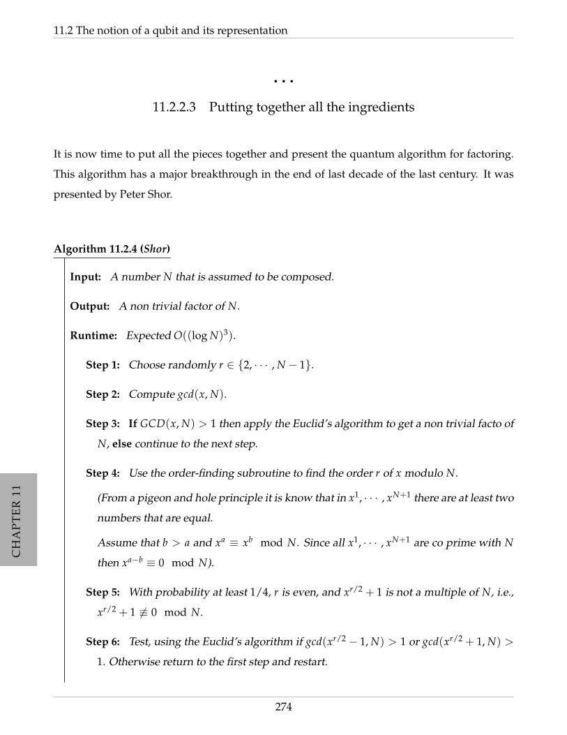
CH

AP

TE

R11

CH

AP

TE

R11

CH

AP

TE

R11

CH

AP

TE

R11

CH

AP

TE

R11

CH

AP

TE

R11

CH

AP

TE

R11

CH

AP

TE

R11

CH

AP

TE

R11

CH

AP

TE

R11


• • •

11.2.2.3 Putting together all the ingredients

It is now time to put all the pieces together and present the quantum algorithm for factoring.

This algorithm has a major breakthrough in the end of last decade of the last century. It was

presented by Peter Shor.

Algorithm 11.2.4 (Shor)

Input: A number N that is assumed to be composed.

Output: A non trivial factor of N.

Runtime: Expected O((log N)3).

Step 1: Choose randomly r ∈ 2, · · · , N − 1.

Step 2: Compute gcd(x, N).

Step 3: If GCD(x, N) > 1 then apply the Euclid’s algorithm to get a non trivial facto of

N, else continue to the next step.

Step 4: Use the order-finding subroutine to find the order r of x modulo N.

(From a pigeon and hole principle it is know that in x1, · · · , xN+1 there are at least two

numbers that are equal.

Assume that b > a and xa ≡ xb mod N. Since all x1, · · · , xN+1 are co prime with N

then xa−b ≡ 0 mod N).

Step 5: With probability at least 1/4, r is even, and xr/2 + 1 is not a multiple of N, i.e.,

xr/2 + 1 6≡ 0 mod N.

Step 6: Test, using the Euclid’s algorithm if gcd(xr/2 − 1, N) > 1 or gcd(xr/2 + 1, N) >

1. Otherwise return to the first step and restart.

274

CH

AP

TE

R11

CH

AP

TE

R11

CH

AP

TE

R11

CH

AP

TE

R11

CH

AP

TE

R11

CH

AP

TE

R11

CH

AP

TE

R11

CH

AP

TE

R11

CH

AP

TE

R11

CH

AP

TE

R11


Notice that if one is fortuned to get randomly a factor of N then there is no need to run the rest

of the algorithm. Step 3 calls the order-finding subroutine, to compute the order r of x modulo

N and is indeed the only part of the algorithm that requires the use quantum computers to be

sufficiently fast, namely to run in polynomial time. The last step completes the algorithm, since

by the next theorem, with probability at least one-half r will be even and xr/2 + 1 6≡ 0 mod N.

Notice that, xr ≡ 1 mod N ⇔ (xr/2)2 ≡ (xr/2 − 1)(xr/2 + 1) ≡ 0 mod N. So applying the

Euclid’s algorithm one can get a non trivial factor of N.

Theorem 11.2.5

Consider a positive integer N and assume that N = pα11 · · · · · p

αmm is composition in primes

of N. Let x be an integer chosen uniformly at random in 1, · · · , N − 1 that is co-prime to

N. If r in the order of x modulo N, then

Pr(r is even and xr/2 ≡ −l mod N) ≥ 1− 12m .

• • •

11.2.2.4 An example of the Shor’s algorithm for n=15

Algorithm 11.2.5

Input: N = 15.

Output: A factor of 15, namely 3 or 5.

Step 1 Choose n = 4 so that 15 < S = 24 = 16.

Step 2 Choose y so that gcd(y, 15) = 1. For example, if y = 13.

Step 3 Initialize two qubit registers to state 0, i.e., |ψ0〉 = |0〉|0〉.

Step 4 Apply Hadamard to the first qubit to get:

|ψ1〉 =1√16

15

∑k=0|k〉|0〉 =

15

∑k=0

14|k〉|0〉

Step 5 Apply unitarily the function f (k) = 13k mod 15 an store t in the second register:

275

CH

AP

TE

R11

CH

AP

TE

R11

CH

AP

TE

R11

CH

AP

TE

R11

CH

AP

TE

R11

CH

AP

TE

R11

CH

AP

TE

R11

CH

AP

TE

R11

CH

AP

TE

R11

CH

AP

TE

R11


|ψ2〉 =14

15

∑k=0|k〉| f (k)〉

Step 6 Apply the quantum Fourier transformation on the first qubit to get:

|ψ3〉 =1

16

15

∑u=0|u〉

15

∑k=0

e2πiuk

16 | f (k)〉

Step 7 Since 13 has period r (unknown in general, in this case 4), the function f is

periodic.

In this case the period happens to divide 16, so that one can write k = m + jr, where

0 < m < r and 0 < j < 16/r, and f (k) can be written as f (m).

Then the new state can be expressed as

|ψ3〉 =1

16

15

∑u=0|u〉

r−1

∑m=0| f (k)〉e

2πium16

16/r−1

∑j=0

e2πiurj

16

=15

∑u=0|u〉bu

r−1

∑m=0| f (k)〉e

2πium16

where bu = 1/r if 16|ur and 0 otherwise.

Step 8 Measure the state of the first register. Let Pu denote the projection onto the state

u, then the probability of observing u is

〈ψ3|Pu|ψ3〉 = r|bu|2 =

1r

if 16|ur

0 otherwise

Step 9 Use u to deduce the value r:

1. If no inference can be made or if r is odd, return to Step 2 and repeat.

2. If r = 2s is even, and ys = −1 mod (15), return to Step 2 and repeat.

3. If gcd(15, js ± 1) > 1, quit;

4. Otherwise, return to Step 2 and repeat.

276

CH

AP

TE

R11

CH

AP

TE

R11

CH

AP

TE

R11

CH

AP

TE

R11

CH

AP

TE

R11

CH

AP

TE

R11

CH

AP

TE

R11

CH

AP

TE

R11

CH

AP

TE

R11

CH

AP

TE

R11


In this case r = 4 and 4|16 the only u’s with a positive probability of being observed

are multiples of 4 ( u = 0, 4, 8, 12), each one occurring at Step 1 with probability 0.25.

Since ur = 16k, for some integer k, one can infer nothing about r if u = 0. The

remaining cases give equations for r of the form r = 4k, r = 2k and 3r = 4k. In the

cases that r and k are relatively prime, the algorithm gives the value of r = 4 for the

period. One knows that value to be correct and that 15 has to divide the product of

132 − 1 and 132 + 1, enabling us to find both of its factors.

If one obtains r = 2, giving values of 12 and 14 for y2 ± l. In this case as the numbers

are so small, one get a factor of 15 in this case, since one of three consecutive numbers

is divisible by 3. However, r = 2 is not the period, and in general we are not guaran-

teed to obtain a factor of N if one gets the wrong value of r. Hence, one can say that

this will be successful in factoring N = 15 at the end of a single run of the procedure

with probability of 1/2.

277

CH

AP

TE

R11

CH

AP

TE

R11

CH

AP

TE

R11

CH

AP

TE

R11

CH

AP

TE

R11

CH

AP

TE

R11

CH

AP

TE

R11

CH

AP

TE

R11

CH

AP

TE

R11

CH

AP

TE

R11


278

CH

AP

TE

R11

CH

AP

TE

R11

CH

AP

TE

R11

CH

AP

TE

R11

CH

AP

TE

R11

CH

AP

TE

R11

CH

AP

TE

R11

CH

AP

TE

R11

CH

AP

TE

R11

CH

AP

TE

R11

Part IV

Applications of Cryptography

279

CH

AP

TE

R11

CH

AP

TE

R11

CH

AP

TE

R11

CH

AP

TE

R11

CH

AP

TE

R11

CH

AP

TE

R11

CH

AP

TE

R11

CH

AP

TE

R11

CH

AP

TE

R11

CH

AP

TE

R11

CH

AP

TE

R11

CH

AP

TE

R11

CH

AP

TE

R11

CH

AP

TE

R11

CH

AP

TE

R11

CH

AP

TE

R11

CH

AP

TE

R11

CH

AP

TE

R11

CH

AP

TE

R11

CH

AP

TE

R11

In this part of this project it is discussed several application of cryptography. Informally

speaking, in this part it is analyzed how one can use the concepts explained in the previous part

for example to sign a document electronically, how one can convince another of the possession

of a secret without revealing the secret, identification processes among others.

281

CH

AP

TE

R11

CH

AP

TE

R11

CH

AP

TE

R11

CH

AP

TE

R11

CH

AP

TE

R11

CH

AP

TE

R11

CH

AP

TE

R11

CH

AP

TE

R11

CH

AP

TE

R11

CH

AP

TE

R11

282

CH

AP

TE

R12

CH

AP

TE

R12

CH

AP

TE

R12

CH

AP

TE

R12

CH

AP

TE

R12

CH

AP

TE

R12

CH

AP

TE

R12

CH

AP

TE

R12

CH

AP

TE

R12

CH

AP

TE

R12

CH

AP

TE

R12

CHAPTER 12

Digital Signtures

The chapter name says it all. Digital signatures are computer/digital based counterpart of legal

handwritten signature in a piece of paper of authentication of electronic records. The purpose

of this chapter is to explain how a digital signature can be created and how it achieves the same

functionality as that of a handwritten signature. The idea is to use asymmetric cryptography

explained in Part III.

The idea of a digital signature is due to Diffie and Hellman that in 1976 described the basic

properties that such scheme must have and conjectured that such schemes could be designed.

Only when Rivest, Shamir, and Adleman proposed RSA as public key cryptographic system,

was possible to design a protocol of digital signature, proving that the concept is sound al-

though it is not secure. In 1988, Goldwasser, Micali, and Rivest rigorously define the security

requirements of digital signature schemes by describing a hierarchy of attack models for signa-

ture schemes, and present the now so called GMR signature scheme, a digital signature scheme

that is proved to be secure even when forged chosen message attack are considered. Nowadays

there are widely marketed software package to offer digital signature such as Lotus Notes (the

first to appear), released in 1989, which used the RSA algorithm.

The reader may wonder why digital signatures are important and what kind of problems

(legal/practical) that one might find when trying to implement such systems. In this chapter it

is not discussed the legal issues that one might find and point out briefly the importance of of

283

CH

AP

TE

R12

CH

AP

TE

R12

CH

AP

TE

R12

CH

AP

TE

R12

CH

AP

TE

R12

CH

AP

TE

R12

CH

AP

TE

R12

CH

AP

TE

R12

CH

AP

TE

R12

CH

AP

TE

R12

CH

AP

TE

R12

them. To illustrate the thematic, first it is presented an example for motivating the discussion

of digital signatures.

Example 12.0.6. Consider the following scenario: a company, an employee (E), the boss (B) and an

email from B informing E of an raise in his salary in the following terms:

Email 12.0.7 (Decision of raising your salary request)

From: [email protected]

To: [email protected]

Dear Collaborator E:

I am delight to inform you that your salary raise has been approved.

Best regards,

Boss B

How can E be sure that this email is for real and how can he convince the human resources department

of that raise? The reader may say “Well there is Boss B name at the end of the message” or “also it came

from Boss B company email”, so this email is for real. But what is the validity of this message? How

does the reader know that this message was not created by someone else in B’s place that had simply had

access to the email sender server?1

Even in the case there was a digital copy of B’s signature what was the validity of the message?

This kind of issues are the base for the study of digital signatures, i.e., process of signing digital

documents without ink based signatures that have “legal” value or more simply compromised

the signer with the document.

Now it is clearer the importance of digital signatures. In the real world, more than ever, the

computer is a tool present in daily life and it is become more and more common one have

1Notice that a similar situation with post mail may happen. The reader can send to a physical letter to his/her

father in the name of the Republic President without its consent saying that him will the awarded a medal. But

in this case, without President’s ink signature, the validity of this message is null. Nowadays the most common

email servers do not allow the sent of an email without being an authorized user.

284

CH

AP

TE

R12

CH

AP

TE

R12

CH

AP

TE

R12

CH

AP

TE

R12

CH

AP

TE

R12

CH

AP

TE

R12

CH

AP

TE

R12

CH

AP

TE

R12

CH

AP

TE

R12

CH

AP

TE

R12

CH

AP

TE

R12

Chapter 12. Digital Signtures

the need to ensure himself about the origin of a message and also when their use is needed

for similar reasons that would use a signature to sign a paper document. The use of ink

signatures or authenticity stamps, digital signatures are no longer a practical to use traditional

signature. Thus, since it is become prominent the digital documents they are the answer

to provide evidences of provenance, identity, and status of an digital document. They also

provide insurance that the content of the message is consented and approved by the one how

signs it. So they become useful tools in many applications such as electronic commerce and

emails for proving the authenticity of messages.

In order to have a digital signature with similar properties to the real signature one must have

the following properties similarly to what one would expect form a handwritten signature:

Authenticity which means that the digital signature would help to assure that the signer

is who he or she claims to be and that can be checked. This is particular important for

example in a financial context. If in a case someone goes into a bank with instructions to

pay a bill and the bank pays it even when the bank collaborator is not convinced of the

provenance of the instruction can be a serious question and a severe mistake.

Integrity which implies that the content has not been changed or tampered since it was

digitally signed, preventing the possibility of a changed after the signing was made

without turning the document into an unsigned one. In particular no one can reuse the

signature to signed new documents without the consent of the sender, which will have to

use its ”pen” to sign the new document.

Non-repudiation in the sense that it proves without error that the signer cannot deny

that he had signed a valid document. This property of digital signatures is crucial for

situations where are conflict between the two parties. For example, one part signs a

contract and the recipient needs to prove to a judge that in fact the first one did indeed

“certify” and signed that contract.

A very important difference between handwrite signature and digital signature is the fact that

in the former case, the signature itself is part of the physical document while in the latter is

not attached physically to the message. So, for that reason the digital signature process has to

“bind” the signature to the message. Another important difference concerns the verification

285

CH

AP

TE

R12

CH

AP

TE

R12

CH

AP

TE

R12

CH

AP

TE

R12

CH

AP

TE

R12

CH

AP

TE

R12

CH

AP

TE

R12

CH

AP

TE

R12

CH

AP

TE

R12

CH

AP

TE

R12

CH

AP

TE

R12

12.1 Definition and examples

process. A conventional signature can be verified by comparison to an other authentic sig-

natures and thus it is not very secure method as it is relatively easy to forge someone else’s

signature. On the other hand digital signatures can be verified by means of publicly known

verification algorithm which everyone can verify making the forgery process much harder.

Public verifiability implies that signatures are transferable, i.e. a signature can be shown to a

third party that also can then verify itself that it has a legitimate signature. These properties,

transferability and public verifiability are essential for the application of digital signatures to

certificates and public-key infrastructures. A third major difference between the two signature

processes mentioned above is the possibility of copy. In the traditional signatures all of them

are distinguishable for each other while in the digital signature, the signatures are all identical

and thus one must be careful in order to prevent a signed digital message from being reused.

For sake of understanding, consider the example where Alice signs a check to pay Bob’s 100

dollars. Of course, Alice wants Bob to be able to do so but it must be the case Bob cannot use

the same check or signature more than once. So the message itself should contain information,

such as a date, which prevents the reusage.

• • • • • • • • • • • • • • • • • • • • • • • • • • • • • • • • • • • • •

SECTION 12.1

Definition and examples

In this section it is presented the definition of digital signature scheme and presented some

examples of such schemes. From the discussion above, one can realize that these type of

schemes must have two basic parts:

Signing process usually an algorithm depending on a private key that binds the signature

to a message that is performed by the person who wants to sign a digital document;

Verification process usually an algorithm depending on a public key that allows anyone to

verify the consistence of the signature.

A possible definition of digital signature is presented next.

286

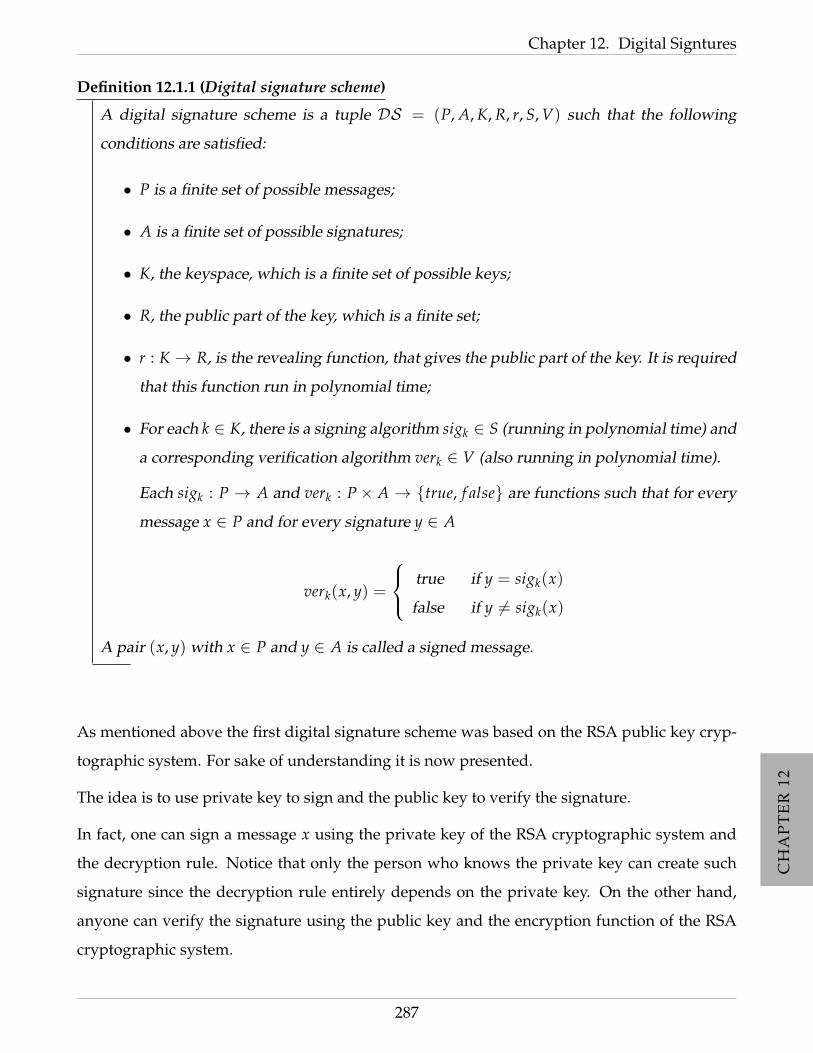
CH

AP

TE

R12

CH

AP

TE

R12

CH

AP

TE

R12

CH

AP

TE

R12

CH

AP

TE

R12

CH

AP

TE

R12

CH

AP

TE

R12

CH

AP

TE

R12

CH

AP

TE

R12

CH

AP

TE

R12

CH

AP

TE

R12


Definition 12.1.1 (Digital signature scheme)

A digital signature scheme is a tuple DS = (P, A, K, R, r, S, V) such that the following

conditions are satisfied:

• P is a finite set of possible messages;

• A is a finite set of possible signatures;

• K, the keyspace, which is a finite set of possible keys;

• R, the public part of the key, which is a finite set;

• r : K → R, is the revealing function, that gives the public part of the key. It is required

that this function run in polynomial time;

• For each k ∈ K, there is a signing algorithm sigk ∈ S (running in polynomial time) and

a corresponding verification algorithm verk ∈ V (also running in polynomial time).

Each sigk : P → A and verk : P× A → true, f alse are functions such that for every

message x ∈ P and for every signature y ∈ A

verk(x, y) =

true if y = sigk(x)

false if y 6= sigk(x)

A pair (x, y) with x ∈ P and y ∈ A is called a signed message.

As mentioned above the first digital signature scheme was based on the RSA public key cryp-

tographic system. For sake of understanding it is now presented.

The idea is to use private key to sign and the public key to verify the signature.

In fact, one can sign a message x using the private key of the RSA cryptographic system and

the decryption rule. Notice that only the person who knows the private key can create such

signature since the decryption rule entirely depends on the private key. On the other hand,

anyone can verify the signature using the public key and the encryption function of the RSA


287

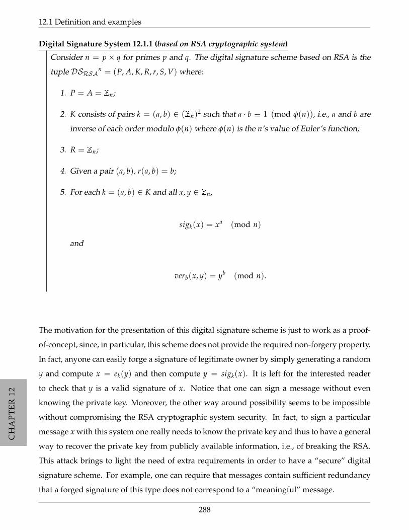
CH

AP

TE

R12

CH

AP

TE

R12

CH

AP

TE

R12

CH

AP

TE

R12

CH

AP

TE

R12

CH

AP

TE

R12

CH

AP

TE

R12

CH

AP

TE

R12

CH

AP

TE

R12

CH

AP

TE

R12

CH

AP

TE

R12

12.1 Definition and examples

Digital Signature System 12.1.1 (based on RSA cryptographic system)

Consider n = p× q for primes p and q. The digital signature scheme based on RSA is the

tuple DSRSAn = (P, A, K, R, r, S, V) where:

1. P = A = Zn;

2. K consists of pairs k = (a, b) ∈ (Zn)2 such that a · b ≡ 1 (mod φ(n)), i.e., a and b are

inverse of each order modulo φ(n) where φ(n) is the n’s value of Euler’s function;

3. R = Zn;


5. For each k = (a, b) ∈ K and all x, y ∈ Zn,

sigk(x) = xa (mod n)

and

verb(x, y) = yb (mod n).

The motivation for the presentation of this digital signature scheme is just to work as a proof-

of-concept, since, in particular, this scheme does not provide the required non-forgery property.

In fact, anyone can easily forge a signature of legitimate owner by simply generating a random

y and compute x = ek(y) and then compute y = sigk(x). It is left for the interested reader

to check that y is a valid signature of x. Notice that one can sign a message without even

knowing the private key. Moreover, the other way around possibility seems to be impossible

without compromising the RSA cryptographic system security. In fact, to sign a particular

message x with this system one really needs to know the private key and thus to have a general

way to recover the private key from publicly available information, i.e., of breaking the RSA.

This attack brings to light the need of extra requirements in order to have a “secure” digital

signature scheme. For example, one can require that messages contain sufficient redundancy

that a forged signature of this type does not correspond to a “meaningful” message.

288

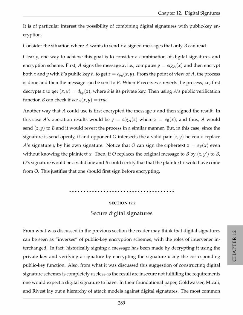
CH

AP

TE

R12

CH

AP

TE

R12

CH

AP

TE

R12

CH

AP

TE

R12

CH

AP

TE

R12

CH

AP

TE

R12

CH

AP

TE

R12

CH

AP

TE

R12

CH

AP

TE

R12

CH

AP

TE

R12

CH

AP

TE

R12


It is of particular interest the possibility of combining digital signatures with public-key en-

cryption.

Consider the situation where A wants to send x a signed messages that only B can read.

Clearly, one way to achieve this goal is to consider a combination of digital signatures and

encryption scheme. First, A signs the message x, i.e., computes y = sigA(x) and then encrypt

both x and y with B’s public key b, to get z = ebB(x, y). From the point of view of A, the process

is done and then the message can be sent to B. When B receives z reverts the process, i.e, first

decrypts z to get (x, y) = dkB(z), where k is its private key. Then using A’s public verification

function B can check if verA(x, y) = true.

Another way that A could use is first encrypted the message x and then signed the result. In

this case A’s operation results would be y = sigA(z) where z = eB(x), and thus, A would

send (z, y) to B and it would revert the process in a similar manner. But, in this case, since the

signature is send openly, if and opponent O intersects the a valid pair (z, y) he could replace

A’s signature y by his own signature. Notice that O can sign the ciphertext z = eB(x) even

without knowing the plaintext x. Then, if O replaces the original message to B by (z, y′) to B,

O’s signature would be a valid one and B could certify that that the plaintext x wold have come

from O. This justifies that one should first sign before encrypting.

• • • • • • • • • • • • • • • • • • • • • • • • • • • • • • • • • • • • •

SECTION 12.2

Secure digital signatures

From what was discussed in the previous section the reader may think that digital signatures

can be seen as “inverses” of public-key encryption schemes, with the roles of intervener in-

terchanged. In fact, historically signing a message has been made by decrypting it using the

private key and verifying a signature by encrypting the signature using the corresponding

public-key function. Also, from what it was discussed this suggestion of constructing digital

signature schemes is completely useless as the result are insecure not fulfilling the requirements

one would expect a digital signature to have. In their foundational paper, Goldwasser, Micali,

and Rivest lay out a hierarchy of attack models against digital signatures. The most common

289

CH

AP

TE

R12

CH

AP

TE

R12

CH

AP

TE

R12

CH

AP

TE

R12

CH

AP

TE

R12

CH

AP

TE

R12

CH

AP

TE

R12

CH

AP

TE

R12

CH

AP

TE

R12

CH

AP

TE

R12

CH

AP

TE

R12

12.2 Secure digital signatures

attacks that one consider for digital signature schemes are:

Key-only attack In this case the attacker is only given the public verification key. I tis the

most general type of attack one can consider.

Message attacks In this kind of attack the enemy is able to examine some signatures corre-

sponding to either known or chosen messages before he tries to break the scheme.

Known message attack Herein the adversary has at hand a list of previously signed mes-

sages. It is a particular case of the previous item where the adversary cannot ask for

signatures of his choice.

Chosen message attack It is a sub-case of second presented item. In this case the adversary

can ask for signatures of documents of his choice. These messages are chosen by the

enemy and are fixed and sent to signing at once, i.e., in a nonadaptive way. Sometimes

this attack is called “generic” since it does not depend on the A’s public key; the same

attack is used against everyone.

Directed Chosen Message Attack This attack is similar to the generic chosen-message at-

tack, except the fact that the list of messages to be signed may be created after the op-

ponent seeing A’s public key but before any signatures are seen. This attack is called

“directed” because it is made against a particular user A.

Adaptive Chosen Message Attack This kind of attack is even more general. In this case

the opponent is also allowed to use A as an “oracle” not only by requesting A signatures

of messages of his choice, that might depend on A’s public key but also request signatures

of messages which depend additionally on previously obtained signatures. It is adaptive

because after each signature obtained the adversary can adaptively choose the next text

to be signed and mount the attack.

In Goldwasser’s, Micali’s, and Rivest’s own words the above list of attacks is ordered increas-

ing by severity in the sense that with the adaptive chosen-message attack is the most general

and natural attack that one can perform. Notice that the adaptive chosen-message attack is

natural and is usually seen in the case of a notary public who must sign more-or-less arbitrary

documents on demand. In general, the user of a signature scheme would like to feel that

290

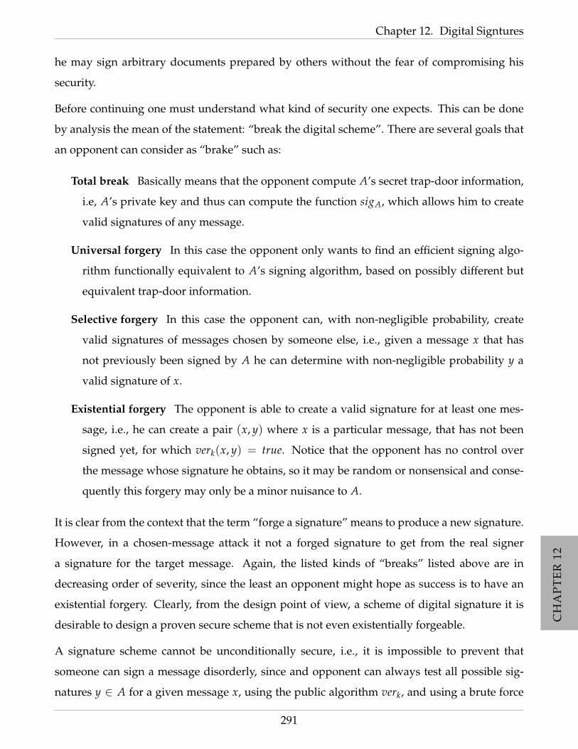
CH

AP

TE

R12

CH

AP

TE

R12

CH

AP

TE

R12

CH

AP

TE

R12

CH

AP

TE

R12

CH

AP

TE

R12

CH

AP

TE

R12

CH

AP

TE

R12

CH

AP

TE

R12

CH

AP

TE

R12

CH

AP

TE

R12


he may sign arbitrary documents prepared by others without the fear of compromising his

security.

Before continuing one must understand what kind of security one expects. This can be done

by analysis the mean of the statement: “break the digital scheme”. There are several goals that

an opponent can consider as “brake” such as:

Total break Basically means that the opponent compute A’s secret trap-door information,

i.e, A’s private key and thus can compute the function sigA, which allows him to create

valid signatures of any message.

Universal forgery In this case the opponent only wants to find an efficient signing algo-

rithm functionally equivalent to A’s signing algorithm, based on possibly different but

equivalent trap-door information.

Selective forgery In this case the opponent can, with non-negligible probability, create

valid signatures of messages chosen by someone else, i.e., given a message x that has

not previously been signed by A he can determine with non-negligible probability y a

valid signature of x.

Existential forgery The opponent is able to create a valid signature for at least one mes-

sage, i.e., he can create a pair (x, y) where x is a particular message, that has not been

signed yet, for which verk(x, y) = true. Notice that the opponent has no control over

the message whose signature he obtains, so it may be random or nonsensical and conse-

quently this forgery may only be a minor nuisance to A.

It is clear from the context that the term “forge a signature” means to produce a new signature.

However, in a chosen-message attack it not a forged signature to get from the real signer

a signature for the target message. Again, the listed kinds of “breaks” listed above are in

decreasing order of severity, since the least an opponent might hope as success is to have an

existential forgery. Clearly, from the design point of view, a scheme of digital signature it is

desirable to design a proven secure scheme that is not even existentially forgeable.

A signature scheme cannot be unconditionally secure, i.e., it is impossible to prevent that

someone can sign a message disorderly, since and opponent can always test all possible sig-

natures y ∈ A for a given message x, using the public algorithm verk, and using a brute force

291

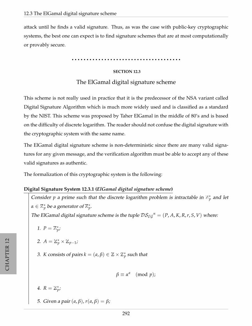
CH

AP

TE

R12

CH

AP

TE

R12

CH

AP

TE

R12

CH

AP

TE

R12

CH

AP

TE

R12

CH

AP

TE

R12

CH

AP

TE

R12

CH

AP

TE

R12

CH

AP

TE

R12

CH

AP

TE

R12

CH

AP

TE

R12

12.3 The ElGamal digital signature scheme

attack until he finds a valid signature. Thus, as was the case with public-key cryptographic

systems, the best one can expect is to find signature schemes that are at most computationally

or provably secure.

• • • • • • • • • • • • • • • • • • • • • • • • • • • • • • • • • • • • •

SECTION 12.3

The ElGamal digital signature scheme

This scheme is not really used in practice that it is the predecessor of the NSA variant called

Digital Signature Algorithm which is much more widely used and is classified as a standard

by the NIST. This scheme was proposed by Taher ElGamal in the middle of 80’s and is based

on the difficulty of discrete logarithm. The reader should not confuse the digital signature with

the cryptographic system with the same name.

The ElGamal digital signature scheme is non-deterministic since there are many valid signa-

tures for any given message, and the verification algorithm must be able to accept any of these

valid signatures as authentic.

The formalization of this cryptographic system is the following:

Digital Signature System 12.3.1 (ElGamal digital signature scheme)

Consider p a prime such that the discrete logarithm problem is intractable in Z∗p and let

α ∈ Z∗p be a generator of Z∗p.

The ElGamal digital signature scheme is the tuple DSEGn = (P, A, K, R, r, S, V) where:

1. P = Z∗p;

2. A = Z∗p ×Zp−1;

3. K consists of pairs k = (a, β) ∈ Z×Z∗p such that

β ≡ αa (mod p);

4. R = Z∗p;

5. Given a pair (a, β), r(a, β) = β;

292

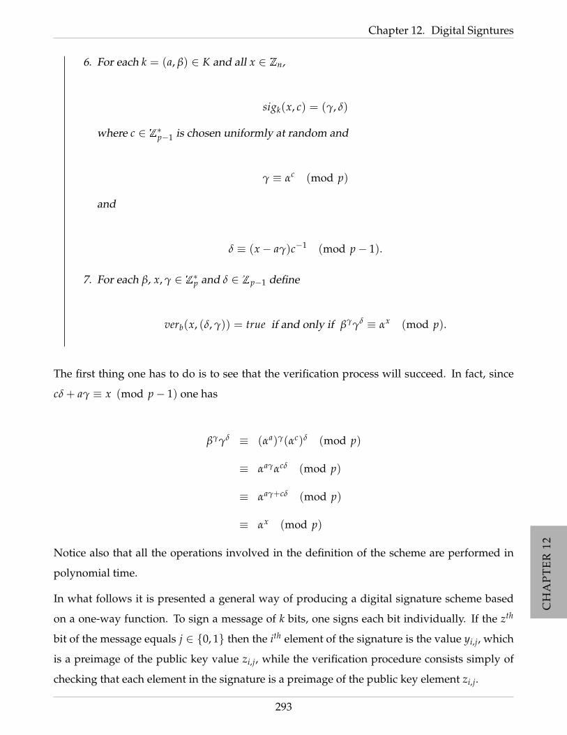
CH

AP

TE

R12

CH

AP

TE

R12

CH

AP

TE

R12

CH

AP

TE

R12

CH

AP

TE

R12

CH

AP

TE

R12

CH

AP

TE

R12

CH

AP

TE

R12

CH

AP

TE

R12

CH

AP

TE

R12

CH

AP

TE

R12


6. For each k = (a, β) ∈ K and all x ∈ Zn,

sigk(x, c) = (γ, δ)

where c ∈ Z∗p−1 is chosen uniformly at random and

γ ≡ αc (mod p)

and

δ ≡ (x− aγ)c−1 (mod p− 1).

7. For each β, x, γ ∈ Z∗p and δ ∈ Zp−1 define

verb(x, (δ, γ)) = true if and only if βγγδ ≡ αx (mod p).

The first thing one has to do is to see that the verification process will succeed. In fact, since

cδ + aγ ≡ x (mod p− 1) one has

βγγδ ≡ (αa)γ(αc)δ (mod p)

≡ αaγαcδ (mod p)

≡ αaγ+cδ (mod p)

≡ αx (mod p)

Notice also that all the operations involved in the definition of the scheme are performed in

polynomial time.

In what follows it is presented a general way of producing a digital signature scheme based

on a one-way function. To sign a message of k bits, one signs each bit individually. If the zth

bit of the message equals j ∈ 0, 1 then the ith element of the signature is the value yi,j, which

is a preimage of the public key value zi,j, while the verification procedure consists simply of

checking that each element in the signature is a preimage of the public key element zi,j.

293

CH

AP

TE

R12

CH

AP

TE

R12

CH

AP

TE

R12

CH

AP

TE

R12

CH

AP

TE

R12

CH

AP

TE

R12

CH

AP

TE

R12

CH

AP

TE

R12

CH

AP

TE

R12

CH

AP

TE

R12

CH

AP

TE

R12

12.3 The ElGamal digital signature scheme

Digital Signature System 12.3.2 (Lamport digital signature scheme)

Consider a positive integer k and assume that f : Y → Z is a one-way function. The

Lamport digital signature scheme the tuple DS = (P, A, K, R, r, S, V) withe following con-

ditions:

• P = 0, 1k;

• A = 0, 1k;

• K, consists of 2k pairs (yi,j, zi,j), where i = 1, · · · k and j = 0, 1 and yi,j ∈ Y and

zi,j = f (yi,j);

• R = 0, 12k, the public part of the key;

• r(yi,j, zi,j) = zi,j;

• For each k = (yi,j, zi,j) ∈ K : i = 1, · · · k, j = 0, 1, and x = (x1, · · · , xk)

sigk(x1, · · · , xk) = (y1,x1 , · · · , yk,xk)

• The verification function is defined as follows. Let (a1, · · · , xk) be a signed message.

Then

verk((x1, · · · , xk), (a1, · · · , xk)) = true⇔ f (ai) = zi,xi

Example 12.3.3. Consider f (x) = 3x (mod 7879) and k = 3. A chooses six ranodm numbers y

i/j 0 1

1 5831 735

2 803 2467

3 4285 6449

the correspondents z’s are:

294

CH

AP

TE

R12

CH

AP

TE

R12

CH

AP

TE

R12

CH

AP

TE

R12

CH

AP

TE

R12

CH

AP

TE

R12

CH

AP

TE

R12

CH

AP

TE

R12

CH

AP

TE

R12

CH

AP

TE

R12

CH

AP

TE

R12


i/j 0 1

1 2009 3810

2 4672 4721

3 268 5731

The sign the message x = (1, 1, 0) one gets (y1,1, y2,1, y3,0) = (735, 2467, 4285).

To verify this signature, it suffices to compute the following:

3735 ≡ 3810 mod 7879

32467 ≡ 4721 mod 7879

34285 ≡ 268 mod 7879

Notice that an opponent cannot forge a signature because he is unable to invert the one-way

function f to obtain the secret y’s. However, the signature scheme can be used to sign only

one message securely. Given signatures on two different messages, it is an easy matter for

the opponent to construct signatures for another message different from the first two (unless

the first two messages differ in exactly one bit). So he can sign 2l − 2 new messages where

l = d(x, x′).

• • • • • • • • • • • • • • • • • • • • • • • • • • • • • • • • • • • • •

SECTION 12.4

The notion of hash function

It is clear from the context of signatures that for practical reasons one cannot use the entire

document to sign a message as at that process would require too much information. Instead

of using all the information of the message one consider a special compression of the message

that works like a fingerprint of the data in such a way that, that similar to a real fingerprint,

identifies uniquely identifies the message. Notice that since the idea is to compress the message

it is impossible to have a uniqueness identification. So instead of uniqueness one requires to

be hard to find two messages that are compressed to the same “fingerprint”. The concretion of

this idea is achieved by the notion of hash function.

Thus, a hash function is an algorithm mapping large data sets of variable length, called keys,

295

CH

AP

TE

R12

CH

AP

TE

R12

CH

AP

TE

R12

CH

AP

TE

R12

CH

AP

TE

R12

CH

AP

TE

R12

CH

AP

TE

R12

CH

AP

TE

R12

CH

AP

TE

R12

CH

AP

TE

R12

CH

AP

TE

R12

12.4 The notion of hash function

to smaller data sets of a fixed length called hash values, hash codes, hash sums, checksums

or simply hashes. In particular, a cryptographic hash function can provide assurance of data

integrity as it provides the data the possibility that if the original data are altered, then the

“fingerprint” will no longer be valid for the original data. The fingerprint is also often referred

to as a message digest and typically is a fairly short string (usually binary with 160 bits).

Usually given a original message x and a changed one, for example, x′ then one expects that y

the digest of x is not also a digest for x′. If this is indeed the case, then the fact that x has been

changed can be detected simply by computing the message digest y′ for x′ and verifying that

y′ 6= y.

A good cryptographic hash function is required to satisfy the following properties:

1. Easy to compute the hash value for any given message;

2. Infeasible to generate a message that has a given hash value;

3. Infeasible to modify a message without changing the hash value;

4. Infeasible to find two different messages with the same hash

With this properties one expect that a cryptographic hash function h should withstand all

known types of cryptographic attacks. In particular it should be:

Preimage resistance: Related with the second item above and also with the concept of one-

way function, since this property makes very unlikely that given y to find any message x

such that y = h(x).

Second-preimage resistance: Related with the third item above states that, given an input x

it should be difficult to find a different input x′ such that h(x) = h(x′). This property is

sometimes called as weak collision resistance.

Collision resistance: Related with the second item above. It states that it is difficult to find

x and x′ such that x 6= x′ and h(x) = h(x′). This kind of pairs are called a hash

collision. This property is also called as strong collision resistance. It imposes that the

hash value has at least twice the length of a hash resistance for preimage-resistance ones

since otherwise collisions may be found by a birthday attack that will be explained in due

course of this section.

296

CH

AP

TE

R12

CH

AP

TE

R12

CH

AP

TE

R12

CH

AP

TE

R12

CH

AP

TE

R12

CH

AP

TE

R12

CH

AP

TE

R12

CH

AP

TE

R12

CH

AP

TE

R12

CH

AP

TE

R12

CH

AP

TE

R12


These properties imply that a malicious adversary cannot replace or modify the input data

without changing its digest and thus, if two messages have the same digest, one can be very

confident that they are identical.

Definition 12.4.1

TBW

Birthday attack...

297

CH

AP

TE

R12

CH

AP

TE

R12

CH

AP

TE

R12

CH

AP

TE

R12

CH

AP

TE

R12

CH

AP

TE

R12

CH

AP

TE

R12

CH

AP

TE

R12

CH

AP

TE

R12

CH

AP

TE

R12

CH

AP

TE

R12

12.4 The notion of hash function

298

CH

AP

TE

R13

CH

AP

TE

R13

CH

AP

TE

R13

CH

AP

TE

R13

CH

AP

TE

R13

CH

AP

TE

R13

CH

AP

TE

R13

CH

AP

TE

R13

CH

AP

TE

R13

CH

AP

TE

R13

CH

AP

TE

R13

CH

AP

TE

R13

CHAPTER 13

Zero knowledge

The concept of zero knowledge conveys the idea of two parties P and V communication to each

other where one has a secret and tries to convince the other that he really knows the secret. One

way that P has to prove to V that we knows the secret is to reveal the secret, but in that case the

secret would no longer be a secret only known by A. So the idea is to use interaction in order

of A to convince V of the “knowledge” of the secret revealing “zero” information about that

secret.

In fact, the zero knowledge requirement is quite stronger than the above explanation. As it

will be clear from the definition presented below, it follows that a protocol will be called “zero

knowledge” if it conveys no information whatsoever about whatever rather than one bit that

is related with the “yes” or “no” quality of the instance that will be explained in due course.

An illustrative example of a Zero Knowledge protocol can presented as follows

Example 13.0.1. Imagine that the reader has one of “Where is Waldo?” comic books and cannot find

the Waldo himself in many pages of the book. We, the writers, on the other hand are experts on this

finding the Waldo in those images and the reader requires our help.

Of course, if we point out the Waldo for the reader in each pictures of the book, then the reader would

lose completely the interest of the book as he could not longer entertain himself looking for Waldo in all

those pictures. Instead, and in order to keep reader’s interest on the book, we could try to convince the

reader that we really are experts on Where’s Waldo book by interacting with the reader and the book to

299

CH

AP

TE

R13

CH

AP

TE

R13

CH

AP

TE

R13

CH

AP

TE

R13

CH

AP

TE

R13

CH

AP

TE

R13

CH

AP

TE

R13

CH

AP

TE

R13

CH

AP

TE

R13

CH

AP

TE

R13

CH

AP

TE

R13

CH

AP

TE

R13

show only Waldo in the picture without revealing his location. To do so we can do the following.

Place in a large table (in fact, 3 times larger than the book) a thick piece of black paper with a very tinny

whole in the center where only the Waldo figure fits in. We kindly ask the reader to turn around and

grab the book, find Waldo and place it in the table in such a way that the Waldo appears in the whole

placed in the paper. Since the entire book in covered we can reveal the reader that in fact Waldo is in the

picture and, moreover, the reader, did not get a clue where, in fact, Waldo is placed in the picture. Again,

we ask the reader to turn around again and take the book under the paper and give it back to the reader

so he can look for Waldo in the same picture we had been shown the Waldo.

If we repeat this procedure a large number of times, at the end, if we manage to show, in each page

chosen by the reader, the Waldo, then the reader will be convinced that, in fact, we are specialists on

finding Waldo without loosing the enthusiasm for search of the character. Another important aspect of

this interactive way of proving is that the reader is convinced that Waldo is really in the picture.

300

CH

AP

TE

R13

CH

AP

TE

R13

CH

AP

TE

R13

CH

AP

TE

R13

CH

AP

TE

R13

CH

AP

TE

R13

CH

AP

TE

R13

CH

AP

TE

R13

CH

AP

TE

R13

CH

AP

TE

R13

CH

AP

TE

R13

CH

AP

TE

R13

Chapter 13. Zero knowledge

Now it is presented the definition of zero knowledge proof system that will be adopted in these

notes.

Definition 13.0.2 (Zero knowledge proof system)

A zero knowledge system between two parties P and V is a protocol involving the P, called

the Prover, and V, called the Verifier, such that P holds a secret s and:

Soundness: If P holds the secret s than he can convince V (up to a negligible probabil-

ity) that he, in fact, holds the secret. This property establishes that in the possession

of the secret there is a way of P to convince V that he knows the secret.

Completeness: If P does not hold the secret then he cannot convince V (with a non

negligible probability) that he has the secret. This property states that if P does not

know the secret no matter what he does V will reject, i.e., will not be convinced of the

possession of the secret by P with significant probability.

Zero knowledgeness: After the end of the protocol, V gets no information whatsoever

about the secret, i.e., the amount of information that V gained during the protocol

is useless to determine the secret s. In particular, the verifier cannot, at the end of

the protocol, convince someone that he knows the secret by trying to impersonate the

prover.

Non-transferability: After the end of the protocol, V cannot prove to a third party that

he was interacting with P. This property aims to prevent a malicious behavior of V

trying to convince another party of the validity of the statement proven by P.

In the next protocols it is presented zero knowledge proof systems for some problems that were

considered in the previous chapter of these notes. In particular, it is designed a zero knowledge

system for the Quadratic Residues, for the Isomorphic graph problem, the Hamiltonian

cycle on graphs (which is an NP complete problem) and for the discrete logarithm. It is also

outlined a way of designing a zero knowledge proof system for any problem in NP based on

the reduction from that language to the Hamiltonian cycle one.

In the first example it is considered the Quadratic Residues problem. For sake of com-

pleteness, and since it is used, in particular, for non prime moduli it is mentioned again its

301

CH

AP

TE

R13

CH

AP

TE

R13

CH

AP

TE

R13

CH

AP

TE

R13

CH

AP

TE

R13

CH

AP

TE

R13

CH

AP

TE

R13

CH

AP

TE

R13

CH

AP

TE

R13

CH

AP

TE

R13

CH

AP

TE

R13

CH

AP

TE

R13

formulation.

Problem 13.0.2 (Quadratic Residues)

Instance: x ∈ Z∗n where n = p× q for some unknown primes p and q;

Question: Is x a quadratic residue modulo n, i.e., is there a u ∈ Z∗n such that u2 ≡ u

(mod n)?

The zero knowledge proof system for this problem is described below. It is assumed that (P, V)

interact with each other and P holds the secret u, a square root of x modulo n.

Protocol 13.0.3 (Zero-knowledge protocol forQuadratic Residues)

Input: An integer n with unknown factorization n = pq, where p and q are prime and x a

quadratic residue modulo n.

Secret: u a square root of x modulo n, i.e., x = u2 (mod n) (unknown to V).

Number of rounds: The following steps are repeated m = log n times.

Step 1: P chooses a random v ∈ Z∗n, and computes y = v2 mod n. P sends y to V.

Step 2: V chooses a random i ∈ 0, 1 and sends it to P as a challenge;

Step 3: P computes z = uiv mod n;

Step 4: V checks if z2 = xiy mod n;

If all rounds are completed with success V accepts that P really knows u, the square root of

x.

Usually, the Step 1 is also known as the commitment step, the Step 1 is also designated as the

challenge step, the Step 3 is also called as the revealing or decommitment step. The Step 4 is

called the verification process.

If x is, in fact, a quadratic residue modulo n and P knows the square root of x modulo n then he

can always answer correctly to V’s challenge. On the other hand if x is a non-quadratic residue

302

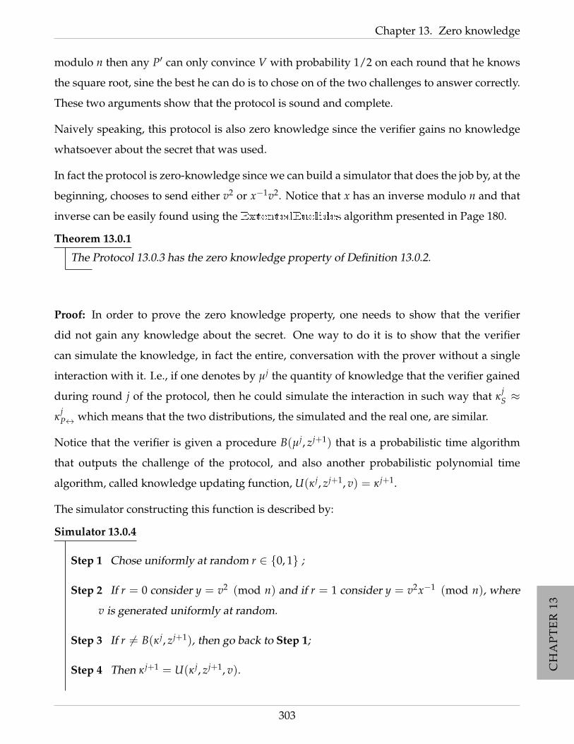
CH

AP

TE

R13

CH

AP

TE

R13

CH

AP

TE

R13

CH

AP

TE

R13

CH

AP

TE

R13

CH

AP

TE

R13

CH

AP

TE

R13

CH

AP

TE

R13

CH

AP

TE

R13

CH

AP

TE

R13

CH

AP

TE

R13

CH

AP

TE

R13


modulo n then any P′ can only convince V with probability 1/2 on each round that he knows

the square root, sine the best he can do is to chose on of the two challenges to answer correctly.

These two arguments show that the protocol is sound and complete.

Naively speaking, this protocol is also zero knowledge since the verifier gains no knowledge

whatsoever about the secret that was used.

In fact the protocol is zero-knowledge since we can build a simulator that does the job by, at the

beginning, chooses to send either v2 or x−1v2. Notice that x has an inverse modulo n and that

inverse can be easily found using the ExtentedEuclides algorithm presented in Page 180.

Theorem 13.0.1

The Protocol 13.0.3 has the zero knowledge property of Definition 13.0.2.

Proof: In order to prove the zero knowledge property, one needs to show that the verifier

did not gain any knowledge about the secret. One way to do it is to show that the verifier

can simulate the knowledge, in fact the entire, conversation with the prover without a single

interaction with it. I.e., if one denotes by µj the quantity of knowledge that the verifier gained

during round j of the protocol, then he could simulate the interaction in such way that κjS ≈

κjP↔ which means that the two distributions, the simulated and the real one, are similar.

Notice that the verifier is given a procedure B(µj, zj+1) that is a probabilistic time algorithm

that outputs the challenge of the protocol, and also another probabilistic polynomial time

algorithm, called knowledge updating function, U(κ j, zj+1, v) = κ j+1.

The simulator constructing this function is described by:

Simulator 13.0.4

Step 1 Chose uniformly at random r ∈ 0, 1 ;

Step 2 If r = 0 consider y = v2 (mod n) and if r = 1 consider y = v2x−1 (mod n), where

v is generated uniformly at random.

Step 3 If r 6= B(κ j, zj+1), then go back to Step 1;

Step 4 Then κ j+1 = U(κ j, zj+1, v).

303

CH

AP

TE

R13

CH

AP

TE

R13

CH

AP

TE

R13

CH

AP

TE

R13

CH

AP

TE

R13

CH

AP

TE

R13

CH

AP

TE

R13

CH

AP

TE

R13

CH

AP

TE

R13

CH

AP

TE

R13

CH

AP

TE

R13

CH

AP

TE

R13

Notice that after m trials, the probability of not reaching Step 4 is (1/2)m and hence, since

B follows a Bernoulli distribution with probability 1/2 then clearly one has κjS ≈ κ

jP↔, as

claimed. This means that if the verifier is capable of generating the proof by himself without

communication with the prover than of course, all that he could gain from the interaction could

also be produced by himself without the interaction.

Now it is discussed the impossibility of transfer the proof. It is shown that is one uses devices

that have non-erasable memory then the verifier can proof to someone else that he interacted

with the prover.

Theorem 13.0.2

If a device with non-erasable memory is given by a third party to V then he can prove that

he had interacted with the prover.

Proof: The proof consists on design of a device D that proves the the interaction. The device is

such that:

• D has a pseudorandom generator with a seed unknown to the verifier.

• D receives a value y and outputs a challenge b and records y and b on its permanent

memory.

• D record the output of the challenge and the acceptance of the verifier.

Since the third party can access to the entire memory of the device then he can conclude if there

was or not interaction between the parties since if the conversation were simulated there are

challenges that were not properly answer and those would require the device to go back and

erase its permanent memory, which is impossible. Thus, the third party got to know if there

was or not communication between the prover and the verifier.

Another example concerning Zero Knowledge is related with NP complete problems. The

reader may ask why this is important and if he thinks for a bit he easily realize that one zero

knowledge protocol for such problem can be used to design a Zero Knowledge protocol for all

NP language. The problem that it is consider here is the Hamiltonian cycle.

304

CH

AP

TE

R13

CH

AP

TE

R13

CH

AP

TE

R13

CH

AP

TE

R13

CH

AP

TE

R13

CH

AP

TE

R13

CH

AP

TE

R13

CH

AP

TE

R13

CH

AP

TE

R13

CH

AP

TE

R13

CH

AP

TE

R13

CH

AP

TE

R13


Problem 13.0.5 (Hamiltonian graphs)

Instance: A graph H;

Question: Is there an Hamiltonian cycle on H, i.e., a sequence that passes through all the

vertices once with the same start and end point?

Before the presentation of the zero knowledge for NP complete problems one needs another

ingredient that plays an important role in this protocol called Commitment schemes. The idea

is to use them to enable a party to commit itself to a value while keeping it secret and in a later

stage the commitment is “opened” and it is guaranteed that the “opening” can yield only a

single value determined in the committing phase.

Heuristically, a commitment scheme is an efficient two-phase two-party protocol through which

one party, called the sender, can commit itself to a value so the following two conflicting

requirements are satisfied.

Secrecy: At the end of the first phase, the other party, called the receiver, does not gain any

knowledge of the sender’s value, even if the receiver tries to cheat.

Unambiguity: Given the transcript of the interaction in the first phase, there exists at most

one value which the receiver may later accept as a legal “opening” of the commitment,

even if the sender tries to cheat.

The first phase is called the commit phase and the second is called the reveal phase. So, to

define a commitment scheme, in first phase it is required that a sender commit itself with a

value and yield no knowledge to the receiver, and in the reveal phase the sender sends to the

receiver the original value and the sequence of random coin tosses that it has used during

the commit phase. The receiver will accept the value if and only if the supplied information

matches its transcript of the interaction in the commit phase.

Before giving the precise definition of bit commitment scheme, we give some preliminaries

definitions:

1. A receiver’s view of an interaction with the sender, denoted (r, m), consists of the random

coins used by the receiver r and the sequence of messages received from the sender m.

305

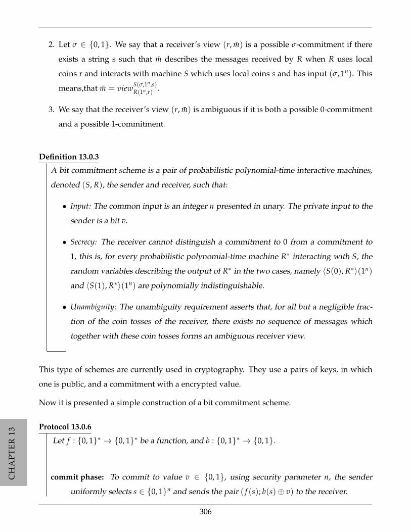
CH

AP

TE

R13

CH

AP

TE

R13

CH

AP

TE

R13

CH

AP

TE

R13

CH

AP

TE

R13

CH

AP

TE

R13

CH

AP

TE

R13

CH

AP

TE

R13

CH

AP

TE

R13

CH

AP

TE

R13

CH

AP

TE

R13

CH

AP

TE

R13

2. Let σ ∈ 0, 1. We say that a receiver’s view (r, m) is a possible σ-commitment if there

exists a string s such that m describes the messages received by R when R uses local

coins r and interacts with machine S which uses local coins s and has input (σ, 1n). This

means,that m = viewS(σ,1n,s)R(1n,r) .

3. We say that the receiver’s view (r, m) is ambiguous if it is both a possible 0-commitment

and a possible 1-commitment.

Definition 13.0.3

A bit commitment scheme is a pair of probabilistic polynomial-time interactive machines,

denoted (S, R), the sender and receiver, such that:

• Input: The common input is an integer n presented in unary. The private input to the

sender is a bit v.

• Secrecy: The receiver cannot distinguish a commitment to 0 from a commitment to

1, this is, for every probabilistic polynomial-time machine R∗ interacting with S, the

random variables describing the output of R∗ in the two cases, namely 〈S(0), R∗〉(1n)

and 〈S(1), R∗〉(1n) are polynomially indistinguishable.

• Unambiguity: The unambiguity requirement asserts that, for all but a negligible frac-

tion of the coin tosses of the receiver, there exists no sequence of messages which

together with these coin tosses forms an ambiguous receiver view.

This type of schemes are currently used in cryptography. They use a pairs of keys, in which

one is public, and a commitment with a encrypted value.

Now it is presented a simple construction of a bit commitment scheme.

Protocol 13.0.6

Let f : 0, 1∗ → 0, 1∗ be a function, and b : 0, 1∗ → 0, 1.

commit phase: To commit to value v ∈ 0, 1, using security parameter n, the sender

uniformly selects s ∈ 0, 1n and sends the pair ( f (s); b(s)⊕ v) to the receiver.

306

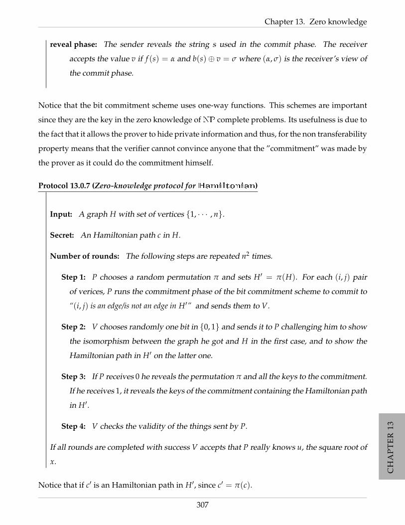
CH

AP

TE

R13

CH

AP

TE

R13

CH

AP

TE

R13

CH

AP

TE

R13

CH

AP

TE

R13

CH

AP

TE

R13

CH

AP

TE

R13

CH

AP

TE

R13

CH

AP

TE

R13

CH

AP

TE

R13

CH

AP

TE

R13

CH

AP

TE

R13


reveal phase: The sender reveals the string s used in the commit phase. The receiver

accepts the value v if f (s) = α and b(s)⊕ v = σ where (α, σ) is the receiver’s view of

the commit phase.

Notice that the bit commitment scheme uses one-way functions. This schemes are important

since they are the key in the zero knowledge ofNP complete problems. Its usefulness is due to

the fact that it allows the prover to hide private information and thus, for the non transferability

property means that the verifier cannot convince anyone that the ”commitment” was made by

the prover as it could do the commitment himself.

Protocol 13.0.7 (Zero-knowledge protocol forHamiltonian)

Input: A graph H with set of vertices 1, · · · , n.

Secret: An Hamiltonian path c in H.

Number of rounds: The following steps are repeated n2 times.

Step 1: P chooses a random permutation π and sets H′ = π(H). For each (i, j) pair

of verices, P runs the commitment phase of the bit commitment scheme to commit to

“(i, j) is an edge/is not an edge in H′” and sends them to V.

Step 2: V chooses randomly one bit in 0, 1 and sends it to P challenging him to show

the isomorphism between the graph he got and H in the first case, and to show the

Hamiltonian path in H′ on the latter one.

Step 3: If P receives 0 he reveals the permutation π and all the keys to the commitment.

If he receives 1, it reveals the keys of the commitment containing the Hamiltonian path

in H′.

Step 4: V checks the validity of the things sent by P.

If all rounds are completed with success V accepts that P really knows u, the square root of

x.

Notice that if c′ is an Hamiltonian path in H′, since c′ = π(c).

307

CH

AP

TE

R13

CH

AP

TE

R13

CH

AP

TE

R13

CH

AP

TE

R13

CH

AP

TE

R13

CH

AP

TE

R13

CH

AP

TE

R13

CH

AP

TE

R13

CH

AP

TE

R13

CH

AP

TE

R13

CH

AP

TE

R13

CH

AP

TE

R13

13.1 Undeniable signatures

The reader is now invited to describe a zero knowledge proof for any NP language. A hint

that helps on the resolution of this task is to notice that, since Hamiltonian is NP com-

plete then this means that there exists a polynomial time reduction from any language to

Hamiltonian, i.e., a polynomial time computable function that not only transforms instances

of the given problem into instances ofHamiltonian but also transform non instances into non

instances ofHamiltonian. Hence, applying the reduction one is able to have a sublanguage of

Hamiltonian to which can apply the above protocol. The details of the design and the proofs

are left as exercise.

• • • • • • • • • • • • • • • • • • • • • • • • • • • • • • • • • • • • •

SECTION 13.1

Undeniable signatures

In the previous Chapter it was discussed digital signatures schemes and it was required that the

signature could be universally verified using the signer’s public key. Although this property is

very convenient in most applications, like e-commerce and digital contracts, one may find

some disadvantages and undesirable consequences in the case of private or commercially

sensitive information. In fact, specially for privacy reasons of the buyer, it is expectable that

one can sign the payment authorization but anyone other than the seller and the bank should

not be convinced that in fact the signer of the payment really allowed that payment. Another

important example, is in the case where compromising authenticated documents are publicly

released.

So, in order to prevent leaked information concerning signers privacy, David Chaum and Hans

van Antwerpen in 1989 came up with the concept of a new kind of signatures, which they

called undeniable signatures, that achieves the required property expressed above. In fact, in

order for the recipient to convince a third party that the signer really signed the document,

needs the cooperation of the signer that interactively provides information, to the third party,

to verify the validity of a signature. This property enables the signer to have control on his

signatures spread by verifying signatures only to concerned or authorized person and every

time someone wants to verify the signatures must interest with him.

On the other hand, to prevent from a malicious signer who would claim that he did not sign a

308

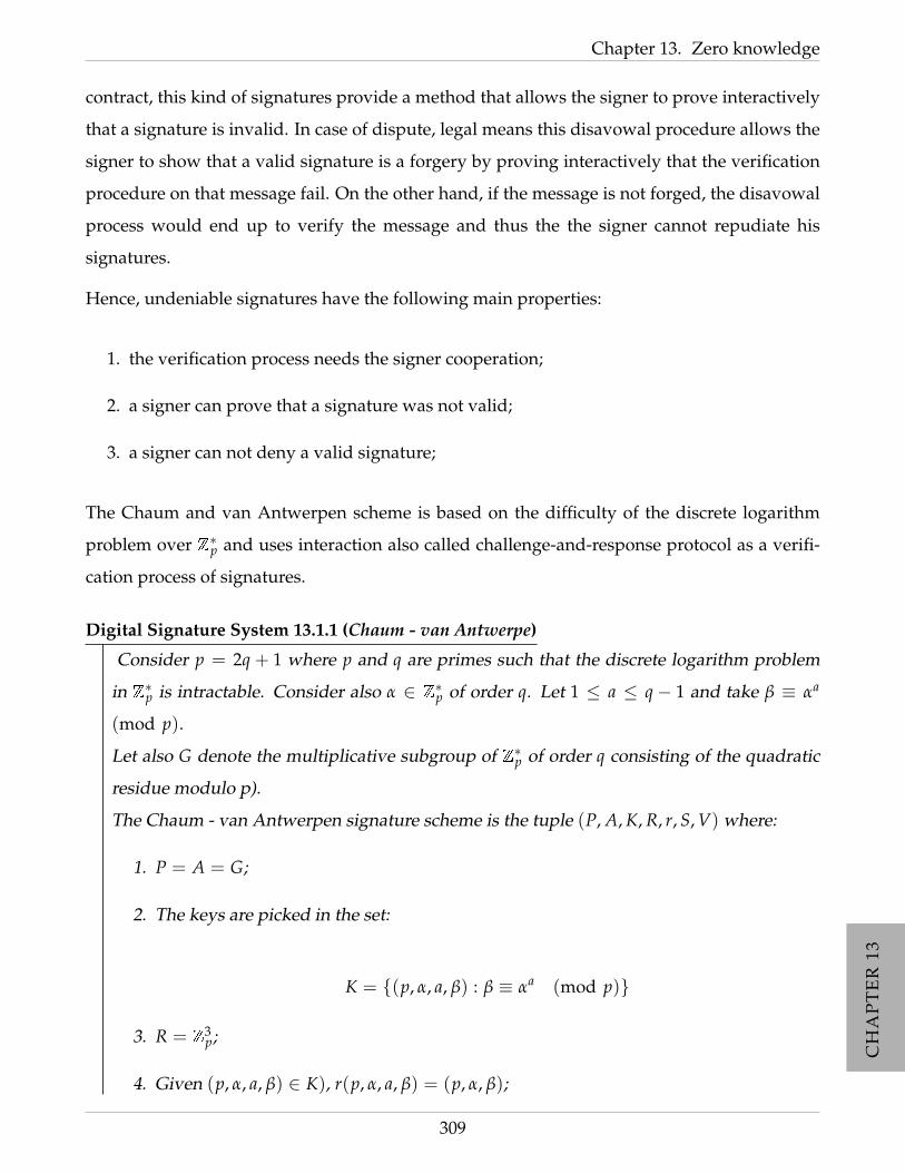
CH

AP

TE

R13

CH

AP

TE

R13

CH

AP

TE

R13

CH

AP

TE

R13

CH

AP

TE

R13

CH

AP

TE

R13

CH

AP

TE

R13

CH

AP

TE

R13

CH

AP

TE

R13

CH

AP

TE

R13

CH

AP

TE

R13

CH

AP

TE

R13


contract, this kind of signatures provide a method that allows the signer to prove interactively

that a signature is invalid. In case of dispute, legal means this disavowal procedure allows the

signer to show that a valid signature is a forgery by proving interactively that the verification

procedure on that message fail. On the other hand, if the message is not forged, the disavowal

process would end up to verify the message and thus the the signer cannot repudiate his

signatures.

Hence, undeniable signatures have the following main properties:

1. the verification process needs the signer cooperation;

2. a signer can prove that a signature was not valid;

3. a signer can not deny a valid signature;

The Chaum and van Antwerpen scheme is based on the difficulty of the discrete logarithm

problem over Z∗p and uses interaction also called challenge-and-response protocol as a verifi-

cation process of signatures.

Digital Signature System 13.1.1 (Chaum - van Antwerpe)

Consider p = 2q + 1 where p and q are primes such that the discrete logarithm problem

in Z∗p is intractable. Consider also α ∈ Z∗p of order q. Let 1 ≤ a ≤ q− 1 and take β ≡ αa

(mod p).

Let also G denote the multiplicative subgroup of Z∗p of order q consisting of the quadratic

residue modulo p).

The Chaum - van Antwerpen signature scheme is the tuple (P, A, K, R, r, S, V) where:

1. P = A = G;

2. The keys are picked in the set:

K = (p, α, a, β) : β ≡ αa (mod p)

3. R = Z3p;

4. Given (p, α, a, β) ∈ K), r(p, α, a, β) = (p, α, β);

309

CH

AP

TE

R13

CH

AP

TE

R13

CH

AP

TE

R13

CH

AP

TE

R13

CH

AP

TE

R13

CH

AP

TE

R13

CH

AP

TE

R13

CH

AP

TE

R13

CH

AP

TE

R13

CH

AP

TE

R13

CH

AP

TE

R13

CH

AP

TE

R13


5. For each k = (p, α, a, β) ∈ K and all x ∈ G,

y = sigk(x) = xa (mod p)

6. For each b = (p, α, β) ∈ R and all x, y ∈ G, the verification procedure is done by the

execution of the following protocol:

Protocol 13.1.2 (Verification Protocol)

Input x, y ∈ G and k the key;

Output Either 1 or 0 is y is a valid signature of x or not.

Step 1 The verifier chooses uniformly at random e1, e2 ∈ Z∗q ;

Step 2 The verifier computes c ≡ ye1 βe2 (mod p) and sends it to signer.

Step 3 The signer computes d ≡ ca−1 (mod q) (mod p) and sends it to the verifier;

Step 4 The verifier accepts y as a valid signature if and only if

d ≡ xe1αe2 (mod p).

First it is necessary to explain why the verifier accepts a valid signature.

Since β ≡ αa (mod p) then βa−1 mod q ≡ α (mod p).

A similar reason applies to y ≡ xa (mod p) to prove ya−1 (mod q) ≡ x (mod p).

Hence:

d ≡ ca−1 mod q (mod p)

≡ ye1a−1 mod qβe2a−1 mod q (mod p)

≡ (ya−1 mod q)e1(βa−1 mod q)e1 (mod p)

≡ xe1αe1 (mod p)

310

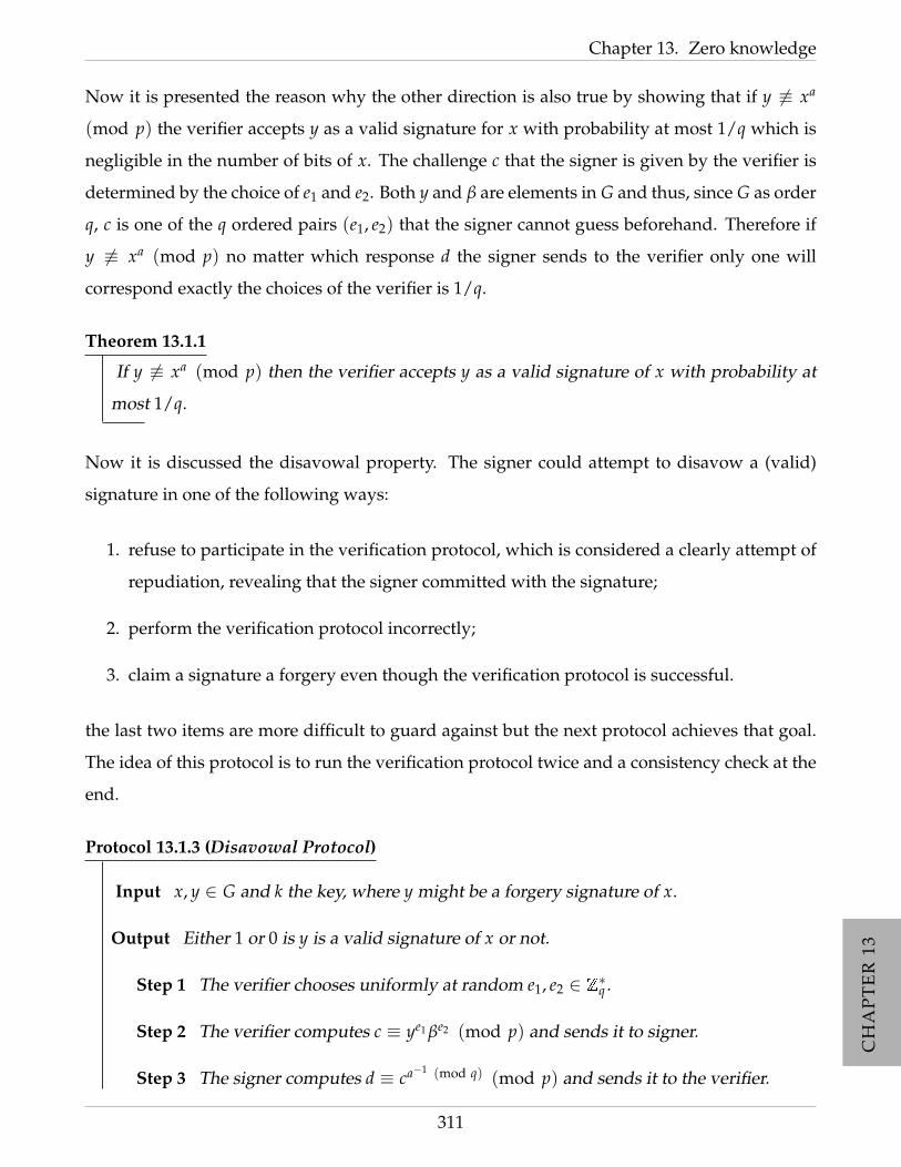
CH

AP

TE

R13

CH

AP

TE

R13

CH

AP

TE

R13

CH

AP

TE

R13

CH

AP

TE

R13

CH

AP

TE

R13

CH

AP

TE

R13

CH

AP

TE

R13

CH

AP

TE

R13

CH

AP

TE

R13

CH

AP

TE

R13

CH

AP

TE

R13


Now it is presented the reason why the other direction is also true by showing that if y 6≡ xa

(mod p) the verifier accepts y as a valid signature for x with probability at most 1/q which is

negligible in the number of bits of x. The challenge c that the signer is given by the verifier is

determined by the choice of e1 and e2. Both y and β are elements in G and thus, since G as order

q, c is one of the q ordered pairs (e1, e2) that the signer cannot guess beforehand. Therefore if

y 6≡ xa (mod p) no matter which response d the signer sends to the verifier only one will

correspond exactly the choices of the verifier is 1/q.

Theorem 13.1.1

If y 6≡ xa (mod p) then the verifier accepts y as a valid signature of x with probability at

most 1/q.

Now it is discussed the disavowal property. The signer could attempt to disavow a (valid)

signature in one of the following ways:

1. refuse to participate in the verification protocol, which is considered a clearly attempt of

repudiation, revealing that the signer committed with the signature;

2. perform the verification protocol incorrectly;

3. claim a signature a forgery even though the verification protocol is successful.

the last two items are more difficult to guard against but the next protocol achieves that goal.

The idea of this protocol is to run the verification protocol twice and a consistency check at the

end.

Protocol 13.1.3 (Disavowal Protocol)

Input x, y ∈ G and k the key, where y might be a forgery signature of x.

Output Either 1 or 0 is y is a valid signature of x or not.

Step 1 The verifier chooses uniformly at random e1, e2 ∈ Z∗q .

Step 2 The verifier computes c ≡ ye1 βe2 (mod p) and sends it to signer.

Step 3 The signer computes d ≡ ca−1 (mod q) (mod p) and sends it to the verifier.

311

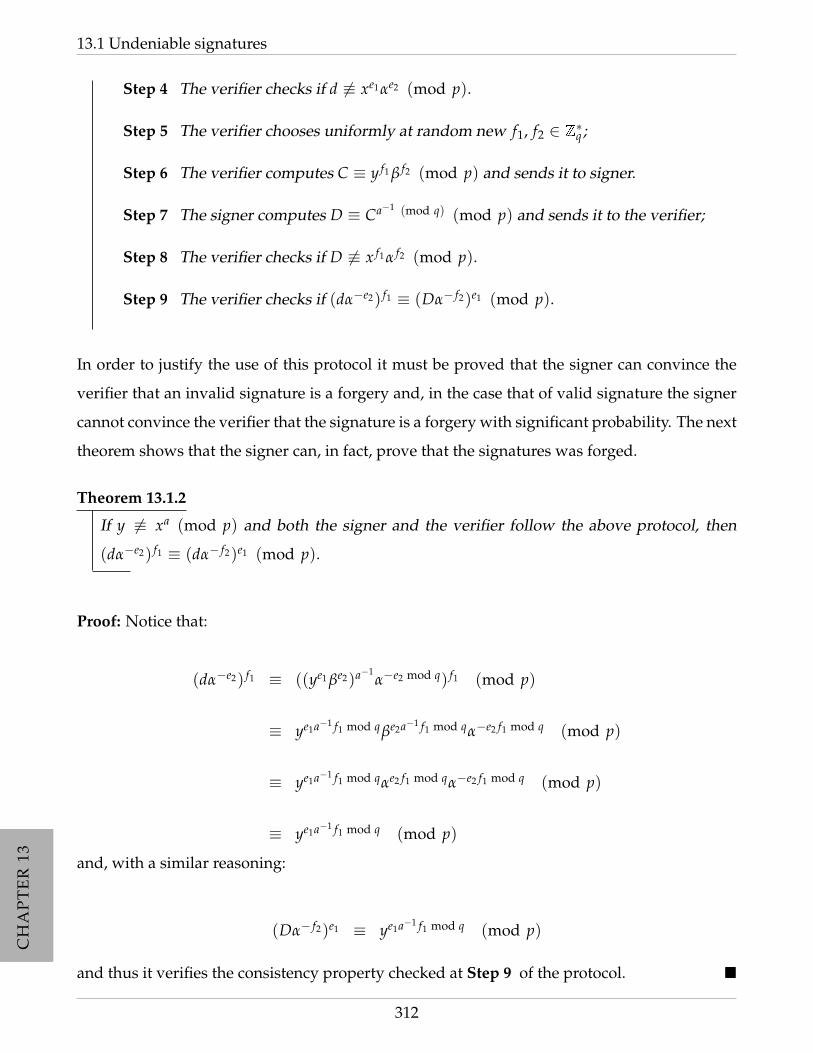
CH

AP

TE

R13

CH

AP

TE

R13

CH

AP

TE

R13

CH

AP

TE

R13

CH

AP

TE

R13

CH

AP

TE

R13

CH

AP

TE

R13

CH

AP

TE

R13

CH

AP

TE

R13

CH

AP

TE

R13

CH

AP

TE

R13

CH

AP

TE

R13


Step 4 The verifier checks if d 6≡ xe1αe2 (mod p).

Step 5 The verifier chooses uniformly at random new f1, f2 ∈ Z∗q ;

Step 6 The verifier computes C ≡ y f1 β f2 (mod p) and sends it to signer.

Step 7 The signer computes D ≡ Ca−1 (mod q) (mod p) and sends it to the verifier;

Step 8 The verifier checks if D 6≡ x f1α f2 (mod p).

Step 9 The verifier checks if (dα−e2) f1 ≡ (Dα− f2)e1 (mod p).

In order to justify the use of this protocol it must be proved that the signer can convince the

verifier that an invalid signature is a forgery and, in the case that of valid signature the signer

cannot convince the verifier that the signature is a forgery with significant probability. The next

theorem shows that the signer can, in fact, prove that the signatures was forged.

Theorem 13.1.2

If y 6≡ xa (mod p) and both the signer and the verifier follow the above protocol, then

(dα−e2) f1 ≡ (dα− f2)e1 (mod p).

Proof: Notice that:

(dα−e2) f1 ≡ ((ye1 βe2)a−1α−e2 mod q) f1 (mod p)

≡ ye1a−1 f1 mod qβe2a−1 f1 mod qα−e2 f1 mod q (mod p)

≡ ye1a−1 f1 mod qαe2 f1 mod qα−e2 f1 mod q (mod p)

≡ ye1a−1 f1 mod q (mod p)

and, with a similar reasoning:

(Dα− f2)e1 ≡ ye1a−1 f1 mod q (mod p)

and thus it verifies the consistency property checked at Step 9 of the protocol.

312

CH

AP

TE

R13

CH

AP

TE

R13

CH

AP

TE

R13

CH

AP

TE

R13

CH

AP

TE

R13

CH

AP

TE

R13

CH

AP

TE

R13

CH

AP

TE

R13

CH

AP

TE

R13

CH

AP

TE

R13

CH

AP

TE

R13

CH

AP

TE

R13


Now it is discussed the (im)possibility of the signer repudiate a valid signature by not perform-

ing trustfully the disavowal protocol. In that case, the signer had to produce d and D such that

the following congruences had to hold:

1. y ≡ xa (mod p);

2. d 6≡ xe1αe2 (mod p);

3. D 6≡ x f1α f2 (mod p);

4. (dα−e2) f1 ≡ (Dα− f2)e1 (mod p).

But then, one would have D ≡ d f10 α f2 (mod p), with d ≡ d1/e1α−e2/e1 (mod p). By Theorem

13.1.1, with probability 1− 1/q, y is a valid signature of d0 and since it is assumed that y is a

valid signature for x, then x ≡ d0 (mod p).

On the other hand, since d 6≡ xe1αe2 (mod p) i.e., x 6≡ d1/e1α−e2/e1 (mod p) ≡ d0 (mod p)

which is a contradiction.

Hence one concludes that:

Theorem 13.1.3

Assume that y ≡ xa (mod p) and the verifier follows the disavowal protocol. If d 6≡ xe1αe2

(mod p) and D 6≡ x f1α f2 (mod p), then the probability that (dα−e2) f1 ≡ (Dα− f2)e1 (mod p)

is at least 1− 1/q.

The idea behind undeniable signatures is similar to a zero knowledge proofs since, for example,

it requires interaction; at the end of the verification procedure the verifier does not gained any

information about the secret of the signer and also he cannot convince anyone else that he had

interact with the prover.

In the sequel it is presented a variation of the undeniable signature in which the verification

and the disavowal protocols are zero knowledge accordingly to Definition 13.0.2.

Consider the Chaum-van Antewerpe undeniable signature presented in Page 309 with the

following protocol for verification:

313

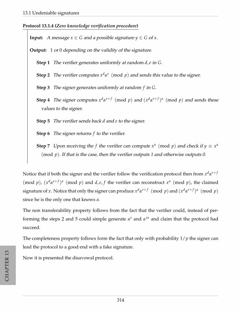
CH

AP

TE

R13

CH

AP

TE

R13

CH

AP

TE

R13

CH

AP

TE

R13

CH

AP

TE

R13

CH

AP

TE

R13

CH

AP

TE

R13

CH

AP

TE

R13

CH

AP

TE

R13

CH

AP

TE

R13

CH

AP

TE

R13

CH

AP

TE

R13


Protocol 13.1.4 (Zero knowledge verification procedure)

Input: A message x ∈ G and a possible signature y ∈ G of x.

Output: 1 or 0 depending on the validity of the signature.

Step 1 The verifier generates uniformly at random d, e in G.

Step 2 The verifier computes xdαe (mod p) and sends this value to the signer.

Step 3 The signer generates uniformly at random f in G.

Step 4 The signer computes xdαe+ f (mod p) and (xdαe+ f )a (mod p) and sends these

values to the signer.

Step 5 The verifier sends back d and e to the signer.

Step 6 The signer returns f to the verifier.

Step 7 Upon receiving the f the verifier can compute xa (mod p) and check if y ≡ xa

(mod p). If that is the case, then the verifier outputs 1 and otherwise outputs 0.

Notice that if both the signer and the verifier follow the verification protocol then from xdαe+ f

(mod p), (xdαe+ f )a (mod p) and d, e, f the verifier can reconstruct xa (mod p), the claimed

signature of x. Notice that only the signer can produce xdαe+ f (mod p) and (xdαe+ f )a (mod p)

since he is the only one that knows a.

The non transferability property follows from the fact that the verifier could, instead of per-

forming the steps 2 and 5 could simple generate αe and αxe and claim that the protocol had

succeed.

The completeness property follows form the fact that only with probability 1/p the signer can

lead the protocol to a good end with a fake signature.

Now it is presented the disavowal protocol.

314

CH

AP

TE

R13

CH

AP

TE

R13

CH

AP

TE

R13

CH

AP

TE

R13

CH

AP

TE

R13

CH

AP

TE

R13

CH

AP

TE

R13

CH

AP

TE

R13

CH

AP

TE

R13

CH

AP

TE

R13

CH

AP

TE

R13

CH

AP

TE

R13


Protocol 13.1.5 (Zero knowledge disavowal procedure)

Input: A message x ∈ G and a possible signature y ∈ G of x and k a number of rounds.

Step 1 The verifier generates uniformly at random d in G and s ∈ 0, · · · , k.

Step 2 The verifier computes xdαs (mod p) and ysαad (mod p) sends this value to the

signer.

Step 3 The signer generates uniformly at random r in G.

Step 3 The signer by trial and error tries to find s. If s is not found chooses s uniformly

at random and using r he commits himself with the value s and send the commitment

to the verifier.

Step 5 The verifier sends back d to the signer.

Step 6 The signer uses d to reconstruct the first message sent and returns r to the

verifier.

Step 7 Upon receiving the f the verifier can compute xa (mod p) and check if y ≡ xa

(mod p). If that is the case, then the verifier outputs 1 and otherwise outputs 0.

The zero knowledge property will be seen in due course...

315

CH

AP

TE

R13

CH

AP

TE

R13

CH

AP

TE

R13

CH

AP

TE

R13

CH

AP

TE

R13

CH

AP

TE

R13

CH

AP

TE

R13

CH

AP

TE

R13

CH

AP

TE

R13

CH

AP

TE

R13

CH

AP

TE

R13

CH

AP

TE

R13


316

CH

AP

TE

R14

CH

AP

TE

R14

CH

AP

TE

R14

CH

AP

TE

R14

CH

AP

TE

R14

CH

AP

TE

R14

CH

AP

TE

R14

CH

AP

TE

R14

CH

AP

TE

R14

CH

AP

TE

R14

CH

AP

TE

R14

CH

AP

TE

R14

CHAPTER 14

Stuff

317

CH

AP

TE

R14

CH

AP

TE

R14

CH

AP

TE

R14

CH

AP

TE

R14

CH

AP

TE

R14

CH

AP

TE

R14

CH

AP

TE

R14

CH

AP

TE

R14

CH

AP

TE

R14

CH

AP

TE

R14

CH

AP

TE

R14

CH

AP

TE

R14

318

CH

AP

TE

R14

CH

AP

TE

R14

CH

AP

TE

R14

CH

AP

TE

R14

CH

AP

TE

R14

CH

AP

TE

R14

CH

AP

TE

R14

CH

AP

TE

R14

CH

AP

TE

R14

CH

AP

TE

R14

CH

AP

TE

R14

CH

AP

TE

R14

Part V

Bibliography

319

CH

AP

TE

R14

CH

AP

TE

R14

CH

AP

TE

R14

CH

AP

TE

R14

CH

AP

TE

R14

CH

AP

TE

R14

CH

AP

TE

R14

CH

AP

TE

R14

CH

AP

TE

R14

CH

AP

TE

R14

CH

AP

TE

R14

CH

AP

TE

R14

CH

AP

TE

R14

CH

AP

TE

R14

CH

AP

TE

R14

CH

AP

TE

R14

CH

AP

TE

R14

CH

AP

TE

R14

CH

AP

TE

R14

CH

AP

TE

R14

CH

AP

TE

R14

CH

AP

TE

R14

CH

AP

TE

R14

CH

AP

TE

R14

Bibliography

[AB09] S. Arora and B. Barak. Computational Complexity - A Modern Approach. Cambridge

University Press, 2009.

[And71] G. Andrews. Number Theory. Dover Publications, Inc, 1971.

[CT91] T. Cover and J. Thomas. Elements of information theory. Wiley-Interscience, New York,

NY, USA, 1991.

[Gol04] Oded Goldreich. The Foundations of Cryptography - Volume 2, Basic Applications.

Cambridge University Press, 2004.

[HPS08] J. Hoffstein, J. Pipher, and J. Silverman. An Introduction to Mathematical Cryptography.

Springer Publishing Company, Incorporated, 1 edition, 2008.

[IR90] K. Ireland and M. Rosen. A Classical Introduction to Modern Number Theory. Graduate

Texts in Mathematics. Springer-Verlag, 1990.

[Kal02] O. Kallenberg. Foundations of Modern Probability. Probability and Its Applications.

Springer, 2002.

[KL07] J. Katz and Y. Lindell. Introduction to Modern Cryptography. Chapman and Hall/CRC

Press, 2007.

[Lan02] S. Lang. Algebra. Springer, 3rd edition, January 2002.

321

CH

AP

TE

R14

CH

AP

TE

R14

CH

AP

TE

R14

CH

AP

TE

R14

CH

AP

TE

R14

CH

AP

TE

R14

CH

AP

TE

R14

CH

AP

TE

R14

CH

AP

TE

R14

CH

AP

TE

R14

CH

AP

TE

R14

CH

AP

TE

R14

Bibliography

[MVO96] A. Menezes, S. Vanstone, and P. Oorschot. Handbook of Applied Cryptography. CRC

Press, Inc., Boca Raton, FL, USA, 1st edition, 1996.

[oST99] National Institute of Standards and Technology. Data Encryption Standard (DES).

FIPS - PUB 46-3, 1999.

[Pap94] C. Papadimitriou. Computational complexity. Addison-Wesley, Reading, Mas-

sachusetts, 1994.

[Sha48] C. Shannon. A mathematical theory of communication. Bell system technical journal,

27, 1948.

[Sip12] M. Sipser. Introduction to the Theory of Computation. Thomson Course Technology,

3rd edition, 2012.

[Sti06] D Stinson. Cryptography: Theory And Practice. The CRC Press Series on Discrete

Mathematics and its Applications. Chapman & Hall/CRC, 2006.

322

notes on cryptography - fenix.tecnico.ulisboa.pt · 9 the rsa cryptographic system 173 ... modern...

Documents