notes on di erential geometry - dma.unifi.it · chapter 1 linear algebra in this chapter we brie y...
TRANSCRIPT
Marco Modugno, Raffaele Vitolo
Notes on Differential Geometry
Notes for studentsDraft of 2014.03.25 - 11.14

2
DiffGeom-2014-03-25.tex; [output 2014-03-25; 11:17]; p.2
CONTENTS
1 Linear Algebra 51.1 Vector spaces . . . . . . . . . . . . . . . . . . . . . . . . . . . . . . . . . . . 5
1.1.1 Vector spaces . . . . . . . . . . . . . . . . . . . . . . . . . . . . . . . 51.1.2 Linear maps . . . . . . . . . . . . . . . . . . . . . . . . . . . . . . . 91.1.3 Multilinear maps . . . . . . . . . . . . . . . . . . . . . . . . . . . . . 111.1.4 Algebras . . . . . . . . . . . . . . . . . . . . . . . . . . . . . . . . . 131.1.5 Symmetric and antisymmetric multilinear maps . . . . . . . . . . . . 151.1.6 Direct sums . . . . . . . . . . . . . . . . . . . . . . . . . . . . . . . 17
1.2 Finite dimensional vector spaces . . . . . . . . . . . . . . . . . . . . . . . . . 201.2.1 Matrices . . . . . . . . . . . . . . . . . . . . . . . . . . . . . . . . . 201.2.2 Square matrices . . . . . . . . . . . . . . . . . . . . . . . . . . . . . 231.2.3 Symmetric and antisymmetric matrices . . . . . . . . . . . . . . . . 241.2.4 Determinant . . . . . . . . . . . . . . . . . . . . . . . . . . . . . . . 261.2.5 Matrix representations . . . . . . . . . . . . . . . . . . . . . . . . . 271.2.6 Transitions of matrix representations . . . . . . . . . . . . . . . . . 291.2.7 Matrix representation of bilinear maps . . . . . . . . . . . . . . . . . 30
1.3 Tensors . . . . . . . . . . . . . . . . . . . . . . . . . . . . . . . . . . . . . . 321.3.1 Tensor product of two vector spaces . . . . . . . . . . . . . . . . . . 321.3.2 Tensor product of several vector spaces . . . . . . . . . . . . . . . . 351.3.3 Tensor representations . . . . . . . . . . . . . . . . . . . . . . . . . . 361.3.4 Tensor algebra . . . . . . . . . . . . . . . . . . . . . . . . . . . . . . 381.3.5 Antisymmetric tensors . . . . . . . . . . . . . . . . . . . . . . . . . 41
1.4 Euclidean spaces . . . . . . . . . . . . . . . . . . . . . . . . . . . . . . . . . 461.4.1 Euclidean spaces . . . . . . . . . . . . . . . . . . . . . . . . . . . . . 461.4.2 Orthogonal maps . . . . . . . . . . . . . . . . . . . . . . . . . . . . 50
1.5 Volume forms . . . . . . . . . . . . . . . . . . . . . . . . . . . . . . . . . . . 521.5.1 Volume forms . . . . . . . . . . . . . . . . . . . . . . . . . . . . . . 521.5.2 Orientation . . . . . . . . . . . . . . . . . . . . . . . . . . . . . . . . 521.5.3 Determinant . . . . . . . . . . . . . . . . . . . . . . . . . . . . . . . 531.5.4 Hodge’s isomorphism . . . . . . . . . . . . . . . . . . . . . . . . . . 551.5.5 Cross product . . . . . . . . . . . . . . . . . . . . . . . . . . . . . . 55
1.6 Affine spaces . . . . . . . . . . . . . . . . . . . . . . . . . . . . . . . . . . . 581.6.1 Action of a group on a set . . . . . . . . . . . . . . . . . . . . . . . 581.6.2 Affine spaces associated with vector spaces . . . . . . . . . . . . . . 591.6.3 Affine spaces associated with groups . . . . . . . . . . . . . . . . . . 63
3
4
2 Differential Geometry 672.1 Manifolds . . . . . . . . . . . . . . . . . . . . . . . . . . . . . . . . . . . . . 672.2 Bundles . . . . . . . . . . . . . . . . . . . . . . . . . . . . . . . . . . . . . . 702.3 Tangent prolongation of manifolds . . . . . . . . . . . . . . . . . . . . . . . 742.4 Tangent prolongation of bundles . . . . . . . . . . . . . . . . . . . . . . . . . 812.5 Connections on bundles . . . . . . . . . . . . . . . . . . . . . . . . . . . . . 832.6 Connections on manifolds . . . . . . . . . . . . . . . . . . . . . . . . . . . . 872.7 Lie Groups . . . . . . . . . . . . . . . . . . . . . . . . . . . . . . . . . . . . 91
2.7.1 Lie Groups . . . . . . . . . . . . . . . . . . . . . . . . . . . . . . . . 912.7.2 Affine spaces associated with Lie groups . . . . . . . . . . . . . . . . 932.7.3 Automorphisms of a vector space . . . . . . . . . . . . . . . . . . . . 94
DiffGeom-2014-03-25.tex; [output 2014-03-25; 11:17]; p.4

CHAPTER 1
LINEAR ALGEBRA
In this chapter we briefly review the fundamental notions of linear algebra thatare used throughout the book.
1.1 Vector spaces
Here, we give the definition and main properties of vector spaces. We introducethe concept of linear map and bilinear map, and study the direct sum splittings.The subject is developed for arbitrary vector spaces; only in the final section wespecialise the above notions to the case of finitely generated vector spaces, which isthe most important case to our purposes.
1.1.1 Vector spaces
1.1.1 Definition. A vector space is defined to be a 3plet (V,+, ·) , where V is anon–empty set, and
+ : V × V → V and · : IR× V → V ,
are two maps which fulfill the following properties:
1. ∀v, w, z ∈ V , we have (v + w) + z = v + (w + z) ,
2. ∃0 ∈ V such that, ∀v ∈ V , we have v + 0 = 0 ,
3. ∀v ∈ V , ∃ − v ∈ V , such that v + (−v) = 0 ,
4. ∀v, w ∈ V , we have v + w = w + v ,
5. ∀v, w ∈ V , λ ∈ IR , we have λ(v + w) = λv + λw ,
6. ∀v ∈ V , λ, µ ∈ IR , we have λ(µv) = (λµ)v ,
7. ∀v ∈ V , λ, µ ∈ IR , we have (λ+ µ)v = λv + µv ,
8. ∀v ∈ V , we have 1v = v .
5

6 Chapter 1. Linear Algebra
1.1.2 Note. As a consequence of the axioms, we obtain
0 v = 0 , for all v ∈ V .
From now on, we will denote a vector space (V,+, ·) by V , by abuse of notation.
1.1.3 Note. Let V be a vector space. A non–empty subset V ′ ⊂ V is said to be avector subspace of V if
v + w ∈ V ′ and λv ∈ V ′ , for all v, w ∈ V ′ , λv ∈ V ′ .
So, a vector subspace V ′ ⊂ V turns out to be a vector space, whose operations + and· coincide with the restriction of the corresponding operations of V .
1.1.4 Note. Let V be a vector space and I a non empty set. A vector v ∈ V is saidto be a linear combination of the vectors bii∈I if there exists a finite family vii∈J ofelements of IR , where J ⊂ I is a finite subset, such that v is equal to the following finitesum of elements of bii∈I
v =∑i∈J
vi bi .
The family bii∈I is said to be independent if the vector 0 is a linear combination ofbii∈I in a unique way, namely, the trivial one.
In other words, if J ⊂ I is a finite subset and vjj∈J is a family of real numbers, then
0 =∑j∈J
vj bj ⇒ vj = 0 , ∀ j ∈ J .
Given a non empty subset S ⊂ V , we define the linear span of S in V to be thefollowing vector subspace of V
span(S) :=∑j∈J
vj xj | vjj∈J ⊂ IR , xjj∈J ⊂ S , J finiteset.
It can be proved that span(S) is the smallest vector subspace (with respect to theinclusion) of V containing S .
1.1.5 Note. Now, suppose that V,W be vector subspaces of a vector space Z . Weobserve that V ∩W is a subspace of Z , while, in general, V ∪W is not a subspace of Z .
We define the following subspace of Z
V +W := span(V ∪W ) =λv + µw | v ∈ V , w ∈ W , λ, µ ∈ IR
.
It can be easily shown that
1. V ∩W is the greatest subspace of Z contained both in V and in W ;
DiffGeom-2014-03-25.tex; [output 2014-03-25; 11:17]; p.6

1.1. Vector spaces 7
2. V +W is the smallest subspace of Z containing V ∪W .
1.1.6 Definition. A non empty subset G ⊂ V is said to be a set of generators ofV if any vector of V is a linear combination of the vectors of G , or, equivalently, ifV = span(G) .
A non empty subset B ⊂ V is said to be a basis if B is a set of independent genera-tors.
It can be shown that any vector space admits a basis. More precisely, the followingTheorem holds.
1.1.7 Theorem. Let V be a vector space, G ⊂ V a set of generators and I ⊂ G anindependent set. Then, there exists a basis B such that
I ⊂ B ⊂ G .
1.1.8 Note. If B is a basis of a vector space V , then each vector of V can be expressedas a linear combination of vectors of B .
Moreover, in virtue of the independence of B , such a linear combination turns outto be unique. Namely, if B = bii∈I and v ∈ V , then v can be uniquely written asv =
∑i∈J v
i bi , where J ⊂ I is a finite subset.
1.1.9 Note. It can be shown that any two bases of the same vector space have thesame cardinality (i.e., the same “number of elements”). Such a cardinality is said to bethe dimension of the vector space.
In particular, a vector space is said to be– finite dimensional if it admits a basis with finite cardinality;– infinite dimensional if it admits a basis with infinite cardinality.In this book, we are mostly concerned with finite dimensional vector spaces.
1.1.10 Note. Any subspace of a finite dimensional vector space Z is a finite dimen-sional vector space, whose dimension is less than or equal to the dimension of the spaceZ .
Suppose that V and W be subspaces of a finite dimensional vector space Z . Then,we have the Grassmann’s formula
dim(V +W ) = dimV + dimW − dim(V ∩W ) .
We have distinguished examples of vector spaces.
1.1.11 Example. The set of real numbers IR is endowed with sum and product whichmake IR a vector space.
We have the distinguished basis 1 of IR ; hence, dim IR = 1 .
1.1.12 Example. Let V and W be two vector spaces. Then, the cartesian productV ×W is endowed with a natural structure of vector space.
DiffGeom-2014-03-25.tex; [output 2014-03-25; 11:17]; p.7

8 Chapter 1. Linear Algebra
Namely, for all x, y ∈ V , z, t ∈ W and λ ∈ IR , we set
+ : (V ×W )× (V ×W )→ V ×W : ((x, z), (y, t)) 7→ (x+ y, z + t) ,
· : IR× (V ×W )→ V ×W : (λ, (x, z)) 7→ (λx, λz) .
It is easily proved that, if B and C are bases of V and W respectively, then B ×C isa basis of V ×W .
1.1.13 Example. Let V be a vector space and W ⊂ V a subspace.Then, we introduce an equivalence relation in V . Namely, if v, v′ ∈ V , then we set
v ∼ v′ ⇔ v − v′ ∈ W .
The quotient set V/W has a natural structure of vector space. We say that V/W isthe quotient vector space.
1.1.14 Example. Let S be a set and V a vector space, and consider the set of maps
Map(S, V ) := f | f : S → V .
The set Map(S, V ) is endowed with a natural structure of vector space, with theoperations + and · defined as follows. For all f, g ∈ Map(S, V ) and all λ ∈ IR we set
f + g : S → V : x 7→ f(x) + g(x) , for all f, g ∈ Map(S, V ) ,
λf : S → V : x 7→ λf(x) , for all λ ∈ IR , f ∈ Map(S, V ) .
The properties of + and · can be easily checked.
1.1.15 Example. Let S be a set. We can define a vector space naturally generatedby S , in the following way.
We define Free(S) to be the set of formal linear combinations of elements of S∑j∈J
vj xj , where J is a finite set, vii∈J ⊂ IR , xii∈J ⊂ S .
In other words, more precisely, we define Free(S) to be the set
Free(S) := f : S → IR | f−1(IR \ 0) finite set ⊂ Map(S, IR) .
The set Free(S) turns out to be equipped with the natural operations of vector space.Even more, we can easily seen that the set Free(S) is a vector subspace of the vectorspace M(S, IR) .
Moreover, if x ∈ S , we define fx ∈ Free(S) to be the map
fx : S → IR : y 7→
1 if y = x
0 if y 6= x.
DiffGeom-2014-03-25.tex; [output 2014-03-25; 11:17]; p.8
1.1. Vector spaces 9
Then, we obtain a natural injection
S → Free(S) : x 7→ fx .
We call Free(S) the free vector space generated by S.One can easily prove that the set S is a basis of Free(S) .
1.1.2 Linear maps
1.1.16 Definition. Let V,W be vector spaces, and f : V → W a map. Then, f issaid to be linear if the following properties hold, for all v, w ∈ V and λ ∈ IR ,
f(v + w) = f(v) + f(w) and f(λv) = λf(v) .
The following result ensures the existence of non trivial linear maps.
1.1.17 Theorem. Let V,W be vector spaces, B ⊂ V a basis of V and f : B → W amap. Then, f can be uniquely extended to a linear map.
Namely, if B = bii∈I and v ∈ V , then v can be uniquely written as v =∑
i∈J vi bi ,
where J ⊂ I is a finite subset and vjj∈J is a family of real numbers, hence the unique
linear extension f of f is determined on v by setting
f(v) = vif(bi) .
1.1.18 Note. Let V and W be vector spaces. With each map f : V → W we canassociate the two subsets
ker f := v ∈ V | f(v) = 0 ⊂ V and im f := w ∈ W | v ∈ V : f(v) = w ⊂ W .
The sets ker f and im f are said to be, respectively, the kernel and the image of f .If f is linear, then ker f is a vector subspace of V and im f is a vector subspace of W .A remarkable property of the kernel of a linear map f is that f is injective if and only
if ker f = 0 .A linear map f : V → W is said to be an isomorphism if it is bijective. In this case,
ker f = 0 and im f = W ,
and f−1 turns out to be linear.
The following important property holds for finite dimensional vector spaces.
1.1.19 Proposition. Let V and W be two finite dimensional vector spaces.For each linear map f : V → W , we have
dimV = dim ker f + dim im f .
DiffGeom-2014-03-25.tex; [output 2014-03-25; 11:17]; p.9

10 Chapter 1. Linear Algebra
1.1.20 Corollary. Two finite dimensional vector spaces are isomorphic if and only ifthey have the same dimension.
Proof. It follows from the above Proposition 1.1.19 and Theorem 1.1.17. QED
1.1.21 Note. If Z is a vector space, and f : V → W and g : W → Z are two linearmaps, then the composition
f g : V → Z : v 7→ f(g(v))
turns out to be a linear map.
1.1.22 Note. The subset
L(V,W ) := f : V → W | f linear ⊂M(V,W )
turns out to be a vector subspace.
1.1.23 Definition. An f ∈ L(V, V ) is said to be an endomorphism of V . We set
End(V ) :=L(V, V ).
1.1.24 Definition. An isomorphism f ∈ End(V, V ) is said to be an automorphismof V . We set
Aut(V ) := f ∈ End(V ) | f automorphism .
1.1.25 Remark. The subset Aut(V ) ⊂ End(V ) is not a vector subspace.On the other hand, Aut(V ) is endowed with the natural structure of (non abelian)
group with respect to the composition of maps.
1.1.26 Definition. We define the dual space of v to be the vector space
V ∗ :=L(V, IR) .
1.1.27 Definition. We define the transpose of the linear map f ∈ L(V,W ) to be thelinear map
f ∗ : W ∗ → V ∗ : α 7→ α f .
We define the transposition to be the linear map
∗ : L(V,W )→ L(W ∗, V ∗) : f 7→ f ∗ .
1.1.28 Note. If Z is a vector space, and f : V → W and g : W → Z are two linearmaps, then we have
(g f)∗ = f ∗ g∗ .
Hence, the transpose of an injective map is surjective and the transpose of a surjectivemap is injective.
DiffGeom-2014-03-25.tex; [output 2014-03-25; 11:17]; p.10

1.1. Vector spaces 11
1.1.29 Note. We have the natural linear map
V → V ∗∗ : v 7→ v∗∗ ,
wherev∗∗ : V ∗ → IR : α 7→ α(v) .
The above map turns out to be injective.We will see that in the finite dimensional case this map is an isomorphism.
1.1.30 Note. We have the natural isomorphism
L(IR, V )→ V : f 7→ f(1) ,
which allows us to make the important identification
L(IR, V ) ' V .
1.1.3 Multilinear maps
Now, we generalise the definition of linear map. Namely, we consider mapsdefined on a cartesian product of vector spaces, and define a multilinear map to bea map which is linear with respect to every factor.
We start by introducing bilinear maps; then, the definition can be easily gener-alised to cartesian products of several vector spaces.
Let us consider three vector spaces V, W, Z .
1.1.31 Definition. A mapf : V ×W → Z
is said to be bilinear if the following properties hold for each v, v′ ∈ V , w,w′ ∈ W ,λ, µ ∈ IR ,
f(λv + µv′, w) = λf(v, w) + µf(v′, w) ,
f(v, λw + µw′) = λf(v, w) + µf(v, w′) .
1.1.32 Note. The above definition admits a further straightforward generalisationto cartesian products of p vector spaces. In this case, we speak of tp–linear map, or ofmultilinear map.
1.1.33 Remark. If f : V ×W → Z is a bilinear map, then f is NOT a linear mapbetween the vector spaces V ×W and Z .
1.1.34 Note. Let f : V ×W → Z be a bilinear map. If v ∈ V and w ∈ W , then weset
f(v, ·) : W → Z : w 7→ f(v, w) and f(·, w) : V → Z : v 7→ f(v, w) .
DiffGeom-2014-03-25.tex; [output 2014-03-25; 11:17]; p.11

12 Chapter 1. Linear Algebra
Clearly, the maps f(v, ·) and f(·, w) are linear.Hence, we obtain the linear maps
fV : V → L(W,Z) : v 7→ f(v, ·) and fW : W → L(V, Z) : w 7→ f(·, w) .
The following result ensures the existence of non trivial bilinear maps.
1.1.35 Theorem. Let V,W,Z be vector spaces, B ⊂ V a basis of V , C ⊂ W a basisof W , and f : B × C → Z a map. Then, f can be uniquely extended to a bilinear map.
Proof. In fact, we recall that B × C turns out to be a basis of V × W . If B = bii∈I andC = cjj∈J , then a vector (v, w) ∈ V ×W can be written as a finite linear combination
(v, w) = (vibi, wjcj) ,
and the unique bilinear extension f of f is determined on (v, w) by setting
f(v, w) = viwj f(bi, cj) .QED
1.1.36 Definition. Let us consider a bilinear map f : V ×W → Z .We define the radicals of f to be the following subspaces of V and W
NV (f) := v ∈ V | f(v, ·) = 0 ≡ ker fV ,
NW (f) := w ∈ W | f(·, w) = 0 ≡ ker fW .
The map f is said to be non degenerate if
NV (f) = 0 and NW (f) = 0 .
A non degenerate bilinear map f : V × W → IR with values in IR is said to be aduality.
1.1.37 Note. A duality f : V ×W → IR yields the linear injections
fV : V → W ∗ : v 7→ fv and fW : W → V ∗ : w 7→ fw .
1.1.38 Definition. Let us consider a duality f : V × W → IR and suppose thatdimV = dimW . Let (bi)i∈I and (ci)i∈I be two bases of V and W , respectively.
We say that (bi) and (ci) are dual bases (with respect to f) if
f(bi, cj) =
1 if i = j ,
0 if i 6= j .
1.1.39 Note. We denote the subset of bilinear maps V ×W → Z by
L2(V,W ; Z) := f : V ×W → Z | f is bilinear ⊂M(V ×W,Z) .
DiffGeom-2014-03-25.tex; [output 2014-03-25; 11:17]; p.12

1.1. Vector spaces 13
Clearly, this subset turns out to be a vector subspace.
1.1.40 Example. A remarkable example of bilinear map is provided by the contrac-tion
〈 , 〉 : V ∗ × V → IR : (α, v) 7→ α(v) .
1.1.41 Note. The contraction is a non degenerate bilinear map.
Proof. 1) If α ∈ V ∗ and f(α, ·) = 0 , then α = 0 , hence NV ∗ = 0 .2) If 0 6= v ∈ V , then there exists a basis B of V such that v ∈ B .Then, we define the map αv : B → IR such that α(w) = 1 if w = v and α(w) = 0 otherwise.We can extend αv to a unique element of V ∗ , which turns out to be non zero.This proves that NV = 0 .QED
1.1.42 Example. The composition of linear maps yields the bilinear map
: L(V,W )× L(W,Z)→ L(V, Z) : (f, g) 7→ g f .
Analogously, if V1, . . . , Vp and Z are vector spaces, then we denote the subset of p–linear (or multilinear) maps V1 × . . .× Vp → Z by
Lp(V1, . . . , Vp;Z) ⊂M(V1 × . . .× Vp; Z) .
In the particular case when V = V1 = · · · = Vp , we set
Lp(V ; Z) :=Lp(V, . . . , V ;Z) .
1.1.4 Algebras
Besides sum and scalar product, it is very useful to consider further algebraicoperations on a vector space. To this aim, we give the following definition.
1.1.43 Definition. Let V be a vector space, and · : V × V → V a bilinear map.Then, we say the pair (V, ·) to be an algebra.
An algebra (V, ·) is said to be
1. associative if, for any v, w, z ∈ V , we have
(v · w) · z = v · (w · z) ;
2. with unity if there exists an element 1V ∈ V such that, for any v ∈ V , we have1V · v = v · 1V = v ;
3. commutative if for any v, w ∈ V , we have v · w = w · v ;
4. anticommutative if, for any v, w ∈ V , we have v · w = −w · v ;
DiffGeom-2014-03-25.tex; [output 2014-03-25; 11:17]; p.13

14 Chapter 1. Linear Algebra
5. a Lie Algebra if it is anticommutative and, for any v, w, z ∈ V , we have
[v, [w, z]] + [z, [v, w]] + [w, [z, v]] = 0 .
Lie algebras are of fundamental importance in many fields of mathematical physics. Inthe second part of this book, we will see concrete examples of Lie algebras in mechanics.
By analogy with the concept of vector subspace, we can introduce the concept ofsubalgebra. Namely, if (V, ·) is an algebra, then a vector subspace W ⊂ V is said to be asubalgebra if the bilinear map · restricts to a bilinear map · : W ×W → W .
Given two algebras, we introduce the class of linear maps between them which “pre-serve” the algebra operations.
1.1.44 Definition. Let (V, (, )) , (W, , ) be an algebra, and f ∈ L(V,W ) . We saythat f is an algebra morphism if, for any v, v′ ∈ V , we have
f((v, v′)) = f(v), f(v′) .
The set of algebra morphisms f ∈ L(V,W ) is a vector subspace of L(V,W ) . Of course,we say that f ∈ End(V ) is an algebra endomorphism if it is an algebra morphism.
Given an algebra, one can consider two further sets of linear endomorphism which“preserve” the algebra operation in a different way from the one above.
1.1.45 Definition. Let (V, (, )) be an algebra and f ∈ End(V ) . We say that f is
1. a derivation of (V, (, )) if, for any v, v′ ∈ V , we have
f((v, v′)) = (f(v), v′) + (v, f(v′)) ;
2. an antiderivation of (V, (, )) if, for any v, v′ ∈ V , we have
f((v, v′)) = (f(v), v′)− (v, f(v′)) .
The set of derivations (antiderivations) f ∈ End(V ) is a vector subspace of End(V ) .
1.1.46 Example. If (V, ·) is an algebra, then we define a new bilinear map
[, ] : V × V → V : (v, w) 7→ [v, w] := v · w − w · v .
It turns out that (V, [, ]) is a Lie algebra. The map [, ] is said to be the commutator,due to the fact that, if (V, ·) is commutative, then [, ] = 0 .
1.1.47 Example. The composition endows the vector space End(V ) with thestructure of associative algebra with the unity idV . This algebra is nor commutativeneither anticommutative. Anyway, End(V ) can be endowed with the commutator, hence(End(V ), [, ]) is a Lie algebra.
DiffGeom-2014-03-25.tex; [output 2014-03-25; 11:17]; p.14

1.1. Vector spaces 15
1.1.48 Example. The space M(V, IR) has a natural structure of associative andcommutative algebra with unity. Namely, we define
· : M(V, IR)×M(V, IR)→M(V, IR) : (f, g) 7→ f · g
where f · g : V → IR : v 7→ f(v)g(v) .
1.1.5 Symmetric and antisymmetric multilinear maps
We introduce the definition and main properties of symmetric and antisymmet-ric multilinear maps. We begin to deal with bilinear maps.
1.1.49 Definition. Let f ∈ L2(V ; IR) . We say f to be symmetric if, for all v, v′ ∈ V ,we have
f(v, v′) = f(v′, v) .
We denote the subset of symmetric bilinear maps by
S2(V, IR) ⊂ L2(V, IR) .
1.1.50 Note. The subset S2(V, IR) ⊂ L2(V, IR) turns out to be a vector subspace.
1.1.51 Note. Let f : V × V → IR be a symmetric bilinear map.We define the linear map
f [ : V → V ∗ : v 7→ f(·, v) ≡ f(v, ·) .
If f is non degenerate, then the map f [ : V → V ∗ is injective.
1.1.52 Definition. Let q : V → IR be a map. Then, q is said to be quadratic if, forall v, w ∈ V and λ ∈ IR ,
q(λv) = λ2q(v) ,
q(v + w)− q(v)− q(w) = 2bq(v, w) ,
where bq : V ×V → IR is a symmetric bilinear map. The set of quadratic maps is a vectorsubspace of the vector space M(V, IR) .
1.1.53 Theorem. [Carnot] Let f : V × V → IR be a symmetric bilinear map. Then,the map
f : V → IR : v 7→ f(v, v)
is quadratic.Indeed, the map f 7→ f is a bijection between the set of symmetric bilinear maps and
the set of quadratic maps. The inverse isomorphism is the map q 7→ f which associateswith every quadratic map q : V → IR the bilinear form
f : V × V → IR : (v, w) 7→ 12
(q(v + w)− q(v)− q(w)
).
DiffGeom-2014-03-25.tex; [output 2014-03-25; 11:17]; p.15

16 Chapter 1. Linear Algebra
1.1.54 Definition. A symmetric bilinear map f ∈ S2(V, IR) is said to be positivedefinite if, for all v ∈ V , with v 6= 0 , we have
f(v, v) > 0 .
1.1.55 Note. Clearly, a positive definite bilinear map is non degenerate.
Note that the set of positive definite maps is not a vector space (even if the sum oftwo positive definite maps is a positive definite map).
1.1.56 Definition. Let f ∈ L2(V ; IR) . We say f to be antisymmetric if, for allv, v′ ∈ V , we have
f(v, v′) = −f(v′, v) .
We denote the subset of antisymmetric bilinear maps by
A2(V, IR) ⊂ L2(V, IR) .
1.1.57 Note. The subset A2(V, IR) ⊂ L2(V, IR) turns out to be a vector subspace.
Now, we generalise the definition of symmetric and antisymmetric map also to mapsin Lp(V ; IR) .
Let us denote by Sp the group of permutations of the set of integers (1, . . . , p) .
A basic example of permutation is an exchange of two elements of (1, . . . , p) . Eachpermutation σ ∈ Sp can be written as the composition of either an even or an odd numberof exchanges. Accordingly, we say a permutation to be even or odd.
If σ ∈ Sp , then we set
|σ| :=
+1 if σ is even
−1 if σ is odd.
1.1.58 Definition. We say a map f ∈ Lp(V, IR) to be, respectively, symmetric, orantisymmetric, if, for all v1, . . . , vp ∈ V and σ ∈ Sr ,
f(σ(v1), . . . , σ(vp)
)= f(v1, . . . , vp) ,
f(σ(v1), . . . , σ(vp)
)= |σ|f(v1, . . . , vp) .
We denote the subsets of symmetric and antisimmetric bilinear maps, respectively, byby
Sp(V, IR) ⊂ Lp(V, IR) and Ap(V, IR) ⊂ Lp(V, IR) .
1.1.59 Note. The subsets Sp(V, IR) ⊂ Lp(V, IR) and Ap(V, IR) ⊂ Lp(V, IR) turn outto be a vector subspaces.
DiffGeom-2014-03-25.tex; [output 2014-03-25; 11:17]; p.16

1.1. Vector spaces 17
1.1.6 Direct sums
1.1.60 Definition. Let Z be a vector space, and V,W ⊂ Z two vector subspaces.
We say that Z splits into the direct sum of V and W if
Z = V +W and V ∩W = 0 .
In such a case, we write
Z = V ⊕W .
We can characterise Z = V ⊕W in the two following equivalent ways.
1.1.61 Theorem. Let Z be a vector space, and V,W ⊂ Z two vector subspaces.
Then, the following conditions are equivalent.
1. Z = V ⊕W .
2. To every z ∈ Z there exists a unique v ∈ V and a unique w ∈ W such that z = v+w .
3. There exist two maps
π1 : Z → V , π2 : Z → W ,
which fulfill
π1|V = idV , π1|W = 0 , π1 + π2 = idZ , π2|V = 0 , π2|W = idW .
Proof. 1) ⇔ 2). Suppose that Z = V ⊕ W and z ∈ Z , v, v′ ∈ V , w,w′ ∈ W , such thatz = v + w = v′ + w′ . Then, v − v′, w − w′ ∈ V ∩W , so that v = v′ and w = w′ .
Conversely, let z ∈ Z , v ∈ V and w ∈W , such that z = v+w . If x ∈ V ∩W , then z = (v−x)+(w+x)is another decomposition of z . It turns out that x = 0 .
2) ⇒ 3). If the second condition holds, then we define the maps π1 and π2 as the unique mapssuch that, for any z ∈ Z , we have z = π1(z) + π2(z) . We can prove that π1 and π2 are linear, and fulfillthe third condition.
3) ⇒ 2). Conversely, if the third condition holds and z ∈ Z , then we have z = π1(z) + π2(z) . Ifv ∈ V and w ∈W such that z = v + w , then π1(z)− v, w − π2(z) ∈ V ∩W . Hence, we have
π1(π1(z)− v) = π1(z)− v = 0 , π2(w − π2(z)) = w − π2(z) = 0 .QED
The maps π1 and π2 are said to be the projections of the splitting Z = V ⊕W .
We have some consequences of the above Theorem together with Theorem 1.1.7.
1.1.62 Corollary. Let Z = V ⊕W . If B is a basis of V and C is a basis of W , thenB ∪ C is a basis of Z .
DiffGeom-2014-03-25.tex; [output 2014-03-25; 11:17]; p.17

18 Chapter 1. Linear Algebra
A basis of Z = V ⊕ W of the above type is said to be a adapted to the splittingZ = V ⊕W .
If Z = V ⊕ W is a finite dimensional vector space, then the Grassmann’s formulayields
dim(V ⊕W ) = dimV + dimW .
1.1.63 Corollary. Let Z be a vector space and V ⊂ Z a vector subspace. Then,there exists a vector subspace W ⊂ Z such that
Z = V ⊕W .
1.1.64 Remark. We stress that the above subspace W above is not uniquely deter-mined.
It is possible to introduce splittings into direct sums of a finite number of vector spacesby means of a straightforward generalisation of our definition. We will make use of suchsplittings in next section.
1.1.65 Example. Let V and W be two vector spaces.We have the two distinguished subspaces of V ×W
V := (v, 0) | v ∈ V and W := (0, w) |w ∈ W .
Clearly, V and W are naturally isomorphic, respectively, to V and W , and we havethe splitting
V ×W = V ⊕ W .
We remark that, in the more general case, in which V and W are just sets, the cartesianproduct V ×W has no distinguished subsets.
1.1.66 Example. We have the splitting
L2(V, IR) = S2(V, IR)⊕ A2(V, IR) .
In fact, we have the two surjective linear maps
S : L2(V, IR)→ S2(V, IR) : f 7→ S(f) ,
A : L2(V, IR)→ A2(V, IR) : f 7→ A(f) ,
where S(f) and A(f) are defined to be the maps
S(f) : V × V → IR : (v, v′) 7→ 12
(f(v, v′) + f(v′, v)) ,
A(f) : V × V → IR : (v, v′) 7→ 12
(f(v, v′)− f(v′, v)) .
Each map f ∈ L2(V, IR) can be written in a unique way as the sum f = S(f) +A(f) .It is worth noting that such a splitting does not hold for p > 2 .
DiffGeom-2014-03-25.tex; [output 2014-03-25; 11:17]; p.18

1.1. Vector spaces 19
1.1.67 Example. We will meet several examples of algebras which have the structureof a direct sum. More precisely, suppose that (V, ·) is an algebra, where
V ≡ ⊕n∈NVn
andv ∈ Vn, v′ ∈ Vm ⇒ v · v′ ∈ Vn+m .
Then, (V, ·) is said to be a graded algebra. Elements of Vn are said to have degree n.It is possible to introduce the notions of graded associative algebras, graded commu-
tative algebras, graded anticommutative algebras and graded Lie algebras. Moreover, itis possible to introduce the concept of graded algebra morphism and graded derivation.
DiffGeom-2014-03-25.tex; [output 2014-03-25; 11:17]; p.19
20 Chapter 1. Linear Algebra
1.2 Finite dimensional vector spaces
In this section, we specialise the definitions and results of the above section tothe case of finite dimensional vector spaces.
In particular, we give the definition and main properties of matrices. The con-ventions on indices and sums that we adopt are often used in mathematical physicsand geometry.
Then, we introduce the matrix representations of finite dimensional vector spaces,and give the matrix representations of some examples from the above section. Theconventions on indices allow us to know the transformation properties of any indexof every matrix representation with respect to any change of basis.
1.2.1 Matrices
In this subsection we give a general definition of matrix, by which we recoverthe usual one.
It is convenient to adopt a positional notation for matrix indexes. The position(upper or lower) of an index will label a transformation property of the index undera change of basis. In concrete examples and computations, this notation will bequite useful.
We introduce an important notation on sums, which allows us to skip the summationsymbol, making formulas more compact and readable. If the same index appears both asa subscript and as a superscript, a sum over the range of the index is understood. Forexample ∑
i∈J
vi bi is denoted by vibi .
Let n ∈ N \ 0 . We set
n := 1, . . . , n
1.2.1 Definition. Let n,m, r, s ∈ N \ 0 .A matrix with r contravariant indices in n and s covariant indexes in m is defined to
be a (partially ordered) family of real numbers
(xi1...ir j1...js) , where i1, . . . , ir ∈ n , j1, . . . jr ∈ m.
We denote by
Mn...nm...m
the set of matrices with r contravariant indexes in n and s covariant indexes in m.
1.2.2 Note. The set Mn...nm...m has a natural structure of vector space. Namely, if
(xi1...ir j1...js), (yh1...hrk1...ks) ∈Mn,...,nm,...,m
DiffGeom-2014-03-25.tex; [output 2014-03-25; 11:17]; p.20

1.2. Finite dimensional vector spaces 21
and λ ∈ IR , then we define the operations + and · as follows
(xi1...ir j1...js) + (yh1...hrk1...ks) := (xi1...ir j1...js + yi1...ir j1...js) ,
λ (xi1...ir j1...js) := (λxi1...ir j1...js) .
1.2.3 Note. More formally, a matrix (xi1...ir j1...js) ∈Mn...nm...m can be regardeded as
the map
x : n× . . .× n×m× . . .×m ≡ nr ×ms → IR : (i1, . . . , ir, j1, . . . , js) 7→ xi1...ir j1...js .
In this way, we have the vector space isomorphism
Mn...nm...m →M(n× . . .×m, IR)
(see Example 1.1.14).
1.2.4 Definition. We define the map
δ : nr × nr → IR :
((a1, . . . , ar), (b1, . . . , br)) 7→ δa1...arb1...br≡
1 (a1, . . . , ar) = (b1, . . . , br)
0 otherwise.
If r = 1 , then δij is said to be the Kronecker’s symbol.Indeed, we have δa1...arb1...br
= δa1b1 . . . δarbr.
1.2.5 Note. We have the distinguished subset of matrices of Mn...nm...m , consisting
of the matrices whose entries vanish all except one.More precisely, for any i1, . . . , ir,∈ n , j1, . . . , js ∈ m, we set
Mi1...irj1...js := (δh1...hri1...ir
δj1...jsk1...ks) ,
The subset of the above matrices turns out to be a natural basis of Mn...nm...m . In
fact, if x := (xi1...ir j1...js) ∈ Mn...nm...m , then we can write x in a unique way as a linear
combination of the vectors Mi1...irj1...js , namely
x = xi1...ir j1...js Mi1...irj1...js .
Hence, we havedimMn...n
m...m = nrms .
1.2.6 Note. It is possible to introduce more general sets of matrices with mixedcovariant and contravariant indexes with different ranges.
For example, the set of matrices (xijk) , with i and k covariant and j contravariant,
and 1 ≤ i ≤ n , 1 ≤ j ≤ m, 1 ≤ k ≤ p , is denoted by Mnmp .
We leave to the reader the task of generalising the above definition.
DiffGeom-2014-03-25.tex; [output 2014-03-25; 11:17]; p.21

22 Chapter 1. Linear Algebra
1.2.7 Note. The vector spaces of matrices are endowed with further natural opera-tions, which we define only in particular cases, leaving to the reader the task of generalisingthem.
1. If x ∈Mmn , and x ∈Mn
p , then we define the (generalised) matrix product
xy ∈Mmnnp
to be((xy)ij
hk) := (xij · yhk) .
The matrix product can be regarded as a bilinear map on the cartesian productMm
n ×Mnp . It is easy to extend the above product to a bilinear map defined on
the cartesian product of any kind of set of matrices.
2. Let z ∈Mmnnp , and i ∈ r , j ∈ s . We define the contraction C2
1(x) of x to be
C21(x) ∈Mm
p , where C21(x) := (xij
jk).
The contraction can be seen as a linear map which is defined, more generally, onsets of matrices with at least a contravariant index and a covariant index rangingon the same set.
1.2.8 Example. We have two kinds of set of matrices with one index, namely Mn
and Mn .If x ≡ (xi) ∈Mn , then we can write x with respect to the natural basis as
x = xiMi .
Equivalently, we write x as the arrayx1
...xn
,
which is said to be a column vector.If y ≡ (yi) ∈Mn , then we can write y with respect to the natural basis as
y = yiMi .
Equivalently, we write y as the array
y = (y1, . . . , yn) ,
which is said to be a row vector.The matrix sets Mn and Mn will be used in the matrix representation of a vector
space and its dual, respectively.
DiffGeom-2014-03-25.tex; [output 2014-03-25; 11:17]; p.22

1.2. Finite dimensional vector spaces 23
1.2.2 Square matrices
Now, we discuss the distinguished particular case of sets of matrices with twoindices.
1.2.9 Definition. We define a square matrix M to be an element of one of thefollowing four vector spaces
Mnm , Mnm , Mn
m , Mnm .
We first consider the vector space Mnm , introducing here some operations.
1.2.10 Note. Let x ≡ (xij) ∈Mnm .
Then, we can write x with respect to the natural basis as
x = xij Mij .
Equivalently, we write the matrix x as a rectangular array, where the first index of thematrix is said to be the row index, and the second index is said to be the column indexx
11 . . . x1m
... . . ....
xn1 . . . xnm
We define the transposition to be the linear map
t :Mnm →Mm
n : (xij) 7→ (xij)t ≡ (xi
j) .
The trasposition turns out to be a linear isomorphism. The transposition can bedefined analogously for Mnm ,Mnm .
We define the trace to be the linear map
C11 :Mn
n → IR : (xij) 7→ xii .
The trace can be defined also for Mnn .
We define the (square) matrix product to be the linear map
Mnm ×Mm
p →Mnp : ((xij), (y
hk)) 7→ (xijy
jk) .
which is the composition of the (generalised) matrix product with the contraction C21 .
The above map coincides with the standard matrix product.
One can do an analogous construction also for Mnm .
1.2.11 Note. In the case m = n , the above map endows Mnn with the structure of
an associative algebra with the unit matrix (δij) .
DiffGeom-2014-03-25.tex; [output 2014-03-25; 11:17]; p.23

24 Chapter 1. Linear Algebra
We denote by
Inn ⊂Mnn
the subset consisting of invertible elements, i.e. the subset of matrices (xi′j) ∈Mn
n suchthat there exists a matrix x−1 ≡ (xij′) ∈Mn
n which fulfills
xi′j x
jj′ = δi
′j′ and xij′ x
j′j = δij .
1.2.12 Note. One can show that, for a given matrix, the maximal number of inde-pendent columns is equal to the maximal number of independent rows. Such a number isdefined to be the rank of the matrix.
It can be shown that a matrix in Mnn is invertible if and only if it is of rank n . The
subset Inn is endowed, by the restriction of matrix product, with a group structure.
1.2.3 Symmetric and antisymmetric matrices
First of all, we consider the vector space Mnn .
1.2.13 Definition. We define the map
ς : nr × nr → IR : ((a1, . . . , ar), (b1, . . . , br)) 7→ ςa1...arb1...br:=∑σ∈Sr
δa1...arbσ(1)...bσ(r).
1.2.14 Note. In particular, let us consider the cases r = 1, 2 .If r = 1 , then ς ij = σij .If r = 2 , then
ς ijhk =
1 if (i, j) = (h, k) or (i, j) = (k, h)
0 if (i, j) 6= (h, k) and (i, j) 6= (k, h) .
1.2.15 Definition. We define the map
ε : nr × nr → IR : ((a1, . . . , ar), (b1, . . . , br)) 7→ εa1...arb1...br:=∑σ∈Sr
|σ|δa1...arbσ(1)...bσ(r).
1.2.16 Note. In particular, let us consider the cases r = 1, 2 and r = n .If r = 1 , then εij = σij .If r = 2 , then
ς ijhk =
1 if (i, j) = (h, k)
−1 if (i, j) = (k, h)
0 if (i, j) 6= (h, k) and (i, j) 6= (k, h) .
If r = n , then we set εi1...in := ε1...ni1...in. .
DiffGeom-2014-03-25.tex; [output 2014-03-25; 11:17]; p.24
1.2. Finite dimensional vector spaces 25
1.2.17 Definition. We define a matrix (xij) ∈ Mnn to be symmetric, or antisym-metric, if, respectively,
xij = xji , or xij = −xji .
1.2.18 Note. The subsets of symmetric and antisymmetric matrices
Snn ⊂Mnn and Ann ⊂Mnn
are vector subspaces.A basis of Snn and a basis of Ann are provided, respectively, by the families of matrices
Sij = (ςhkij ) , 1 ≤ i ≤ j ≤ n ,
Aij = (εhkij ) , 1 ≤ i < j ≤ n .
Thus, we have
dimSnn = 12
(n2 + n) and dimAnn = 12
(n2 − n) .
We have the splitting
Mnn = Snn ⊕Ann .
In fact, we have the linear maps
S :Mnn → Snn : (xij) 7→ S(xij) and A :Mnn → Ann : (xij) 7→ A(xij) ,
where
S(xij) := 12
(xij + xji) , and A(xij) := 12
(xij − xji) .
Hence,
S(xij) + A(xij) = (xij) .
Now, we generalise the definition of symmetric and antisymmetric square matrices tomatrices in Mn...n , with r covariant indices.
1.2.19 Definition. We say a matrix (xi1...ir) ∈Mn...n to be
1. symmetric if, for any σ ∈ Sr , we have
xσ(i1)...σ(ir) = xi1...ir ;
2. antisymmetric if, for any σ ∈ Sr , we have
xσ(i1)...σ(ir) = |σ|xi1...ir .
DiffGeom-2014-03-25.tex; [output 2014-03-25; 11:17]; p.25

26 Chapter 1. Linear Algebra
1.2.20 Note. The subsets of symmetric and antisymmetric matrices
Sn...n ⊂Mn...n and An...n ⊂Mn...n
are vector subspaces.
A basis of Sn...n and a basis of An...n are provided, respecctively, by the families ofmatrices
Si1...ir = (ςh1...hri1...ir) , 1 ≤ i1 ≤ · · · ≤ ir ≤ n ,
Ai1...ir = (εh1...hri1...ir) , 1 ≤ i1 < · · · < ir ≤ n .
Thus,
dimSn...n =
(n+ r − 1
r
)and dimAn...n =
(n
r
).
Hence,
1) dimSn...n is an increasing sequence in r converging to +∞ ;
2) dimAn...n = 1 , for r = n , and dimAn...n = 0 , for r > n .
Moreover, for r = n , we have
A1...n = εi1...in Mi1...in .
An analogous construction can be done for the space Mn...n .
1.2.21 Remark. We stress that the splitting of Mn...n into the direct sum of sym-metric and antisymmetric matrices holds only in the case r = 2 .
1.2.4 Determinant
We give the definition of the determinant of a square matrices.
1.2.22 Note. We identifyMnn withMn×. . .×Mn by means of the following natural
isomorphism
Mnn →Mn × . . .×Mn : (xij) 7→ (xi1, . . . , x
in) .
The matrix A1...n = (εi1...in) yields the antisymmetric n–linear map
Mn × . . .×Mn → IR : (xi1 , . . . , xin) 7→ εi1...in xi1 · · ·xin .
1.2.23 Definition. We define the determinant to be the antisymmetric n–linear map
det :Mnn → IR : (xij) 7→ εi1...in x
i11, . . . , x
inn
The determinant has the following characterisation.
DiffGeom-2014-03-25.tex; [output 2014-03-25; 11:17]; p.26
1.2. Finite dimensional vector spaces 27
1.2.24 Proposition. The determinant is the unique antisymmetric n–linear map ofthe type
det :Mnn → IR ,
such thatdet(δij) = 1 .
Proof. The vector space of antisymmetric n–linear maps Mn × . . . ×Mn → IR has dimension 1 ,hence such a map is characterised by its value on an n–tuple of non–zero vectors. QED
1.2.25 Corollary. If A,B ∈Mnn , then we have det(AB) = detA detB .
Proof. The two antisymmetric n–linear maps
det(A·) :Mnn → IR : B 7→ det(AB) and det(A) det · :Mn
n → IR : B 7→ det(A) det(B)
assume the same value on the matrix B = (δij)) , as
det(A (δij)) = det(A) det(δij) .
Hence, the two n–linear maps det(A·) and det(A) det · coincide. QED
Analogously, we can define the determinant for elements of Mnn , or Mnn , or Mnn .
1.2.5 Matrix representations
In this subsection, we show that, for each finite dimensional vector space, thechoice of a basis yields an isomorphism with a vector space of matrices. This iso-morphism is said to be a matrix representation of the vector space.
We show also that a matrix representation of a vector space yields also matrixrepresentations of the dual space, of the space of endomorphisms, and so on.
Let us consider the finite dimensional vector spaces V,W,Z , respectively, with di-mensions
dimV = n , dimW = p , dimZ = q .
Moreover, we assume the ordered bases
(bi)1≤i≤n ⊂ V , (cj)1≤j≤p ⊂ W , (dk)1≤k≤q ⊂ Z .
1.2.26 Proposition. We have the matrix representation
V →Mn : vi bi 7→ (vi) .
Proof. It is an obvious consequence of Theorem 1.1.17 and Proposition 1.1.19. QED
We stress that a change of the basis, or even a change of the order of a basis, yields adifferent matrix representation.
A matrix representation of V induced by (bi) yields a matrix representation of V ∗ .
DiffGeom-2014-03-25.tex; [output 2014-03-25; 11:17]; p.27

28 Chapter 1. Linear Algebra
1.2.27 Lemma. For 1 ≤ i ≤ n , let us denote by βi ∈ V ∗ the unique linear extensionof the map
βi : (bj)→ IR : bj 7→ βi(bj) = δij .
Then, (βi) turns out to be a basis of V ∗ .
Proof. In fact, any linear map α : V → IR is uniquely determined by its restriction to the subset(bi) ⊂ V .
Hence, we can write α = α(bi)βi , where the components α(bi) are uniquely determined. QED
1.2.28 Proposition. We have the matrix representation of V ∗
V ∗ →Mn : α 7→ (αi) ≡(α(bi)
).
Hence, dimV = dimV ∗ . Therefore, V and V ∗ are (not naturally) isomorphic.
1.2.29 Note. If V is finite dimensional, then we have
dimV = dimV ∗∗
and a natural linear isomorphism (see Note 1.1.29)
V → V ∗∗ .
In what follows, we denote by (γj)1≤j≤p and (δk)1≤k≤q the dual bases of W and Z ,respectively.
1.2.30 Proposition. We have the matrix representation
L(V,W )→Mpn : f 7→
(γj(f(bi)
).
Hence, dimL(V,W ) = dimV · dimW .
1.2.31 Corollary. Let f ∈ L(V,W ) and h ∈ L(W,Z) . Moreover, suppose that(f j i) ∈Mp
n and (hkj) ∈Mqp be their matrix representations.
Then the matrix representation of h f is the matrix product of (hkj) with (f j i) , i.e.
((h f)ki) = (hkj fji) .
1.2.32 Note. In particular, we observe that the Kronecker’s symbol is the matrixrepresentation of idV ∈ EndV .
Hence, the matrix representation
End(V )→Mnn
is an isomorphism of associative algebras with unity, which restricts to a group isomor-phism
Aut(V )→ Inn .
DiffGeom-2014-03-25.tex; [output 2014-03-25; 11:17]; p.28
1.2. Finite dimensional vector spaces 29
1.2.33 Definition. We define the rank of f ∈ L(V,W ) to be the dimension of thevector subspace im f ⊂ W .
1.2.34 Note. The rank of f ∈ L(V,W ) is equal to the rank of the matrix whichcorresponds to f with respect to the given bases in V and W .
1.2.35 Note. If f ∈ L(V,W ) , then the matrix representation of f induces the linearmap
f :Mn →Mp : (vi) 7→ (vi f j i) ,
which is the unique linear map which makes the following diagram commute
Vf- W
Mn? (f)
-Mp?
1.2.36 Note. Let f ∈ L(V,W ) . Then, f ∗ : W ∗ → V ∗ is represented, with respect tothe dual bases, by the matrix (fi
j) ∈Mpn , which is the transpose of the matrix (f j i) .
1.2.6 Transitions of matrix representations
Next, we discuss the effect of a change of the basis on the matrix representationof vectors and linear maps.
Let us consider a vector space V with finite dimension dimV = n .
Moreover, let us consider two ordered bases of V and the dual bases of V ∗
(bi)1≤i≤n and (b′j)1≤j≤n ,
(βi)1≤i≤n and (β′j)1≤j≤n .
1.2.37 Note. We can express, in a unique way, the vectors of each of the two bases,and of their dual bases, as linear combination of the vectors of the other basis as follows
b′i = B′ij bj and bi = Bi
j b′j ,
β′i = C ′ij βj and βi = Ci
j β′j .
1.2.38 Definition. We say (B′ij) , (Bi
j) , (C ′ij) and (Cij) to be the transition matrices
between, respectively the bases (bi) and (b′i) and the dual bases (βi) and (β′i) .
1.2.39 Proposition. The transition matrices are invertible and we have
(Bij)−1 = (B′i
j) = (Cij) and (Ci
j)−1 = (C ′ij) = (Bi
j) .
DiffGeom-2014-03-25.tex; [output 2014-03-25; 11:17]; p.29

30 Chapter 1. Linear Algebra
1.2.40 Corollary. The transition from the basis (bi) to the basis (bi′) induces thefollowing transitions of matrix representations of V and V ∗
v′i = vj Bji and vi = v′j B′j
i ,
α′i = B′ij αj and αi = Bi
j α′j .
1.2.41 Remark. Let us consider the matrix representation of End(V )
End(V )→Mnn : f 7→ (f j i) .
induced by the basis (bi) in the domain and the basis (b′i) in the codomain.This is an isomorphism of vector spaces, but it is not an isomorphism of associative
algebras with unity.In fact, it does not preserve the product of matrices and the matrix representation of
idV is
idV 7→ Bij .
1.2.42 Note. The following practical rule about change of bases holds for matrixrepresentations of any vector space:
- contravariant indices transform by multiplication with the matrix of the change ofbasis,
- covariant indices transform by multiplication with the transpose of the inverse matrixof the change of basis.
This rule shows the advantages coming from our notation, making very easy to eval-uate the effect of a change of basis on a matrix representation.
1.2.7 Matrix representation of bilinear maps
We end this section with the matrix representation of bilinear maps.
Let us consider the finite dimensional vector spaces V,W,Z , respectively with dimen-sions
dimV = n , dimW = p , dimZ = q .
Moreover, we assume the ordered bases and their dual bases
(bi)1≤i≤n ⊂ V , (cj)1≤j≤p ⊂ W , (dk)1≤k≤q ⊂ Z ,
(βi)1≤i≤n ⊂ V ∗ , (γj)1≤j≤p ⊂ W ∗ , (δk)1≤k≤q ⊂ Z∗ .
Then, the induced basis of the cartesian product vector space V ×W is
(bi, cj) 1 ≤ i ≤ n , 1 ≤ j ≤ p .
Thus, we have dimV ×W = dimV dimW .
DiffGeom-2014-03-25.tex; [output 2014-03-25; 11:17]; p.30

1.2. Finite dimensional vector spaces 31
1.2.43 Proposition. We have the matrix representation
L2(V,W ;Z)→Mqnp : f 7→ (fkij) = δk
(f(bi, cj)
).
Thus, we have dimL(V,W ;Z) = dimV dimW dimZ .
1.2.44 Example. We have the matrix representation
L2(V ∗, V ; IR)→Mnn : f 7→ (f j i) :=
(f(βj, bi)
).
The contraction (see Example 1.1.40) turns out to have the matrix representation
(δji ) = (〈βj, bi〉) ∈Mnn .
1.2.45 Example. We have the matrix representation
L2(V ; IR)→Mnn : f 7→ (fij) :=(f(bi, bj)
).
Moreover, f is symmetric (antisymmetric) if and only if
fij = fji (fij = −fji) .
Hence, we have the matrix representations
S2(V ; IR)→ Snn and A2(V ; IR)→ Ann ,
and, more generally, we have the matrix representations
Sr(V ; IR)→ Sn...n and Ar(V ; IR)→ An...n .
DiffGeom-2014-03-25.tex; [output 2014-03-25; 11:17]; p.31
32 Chapter 1. Linear Algebra
1.3 Tensors
Tensor products are used in mechanics and field theory because they providea very convenient way of representing linear and multilinear maps between finitedimensional vector spaces. By means of tensor products it is easy to perform oper-ations in a coordinate free way, such that contractions and determinant.
In this section, we give a brief outline of the general construction of tensorproducts between (possibly infinite dimensional) vector spaces. Then, we show howtensor products yield a way of representing spaces of linear and multilinear maps.
Using this representation we identify several vector spaces of maps which arenaturally isomorphic to a single tensor product of vector spaces. Hence, tensorproducts will be distinguished representatives in any class of naturally isomorphicspaces of linear and multilinear maps.
1.3.1 Tensor product of two vector spaces
In this subsection, we give the definition of tensor product of two vector spacesV,W as a vector space arising naturally from the cartesian product V ×W .
Then, we show that the tensor product is uniquely characterised by means of a“universal property”.
Let us consider two vector spaces V,W .
We consider the free vector space generated by V ×W (see Example 1.1.15)
Free(V ×W ) := f : V ×W → IR := Map(V ×W, IR) .
Moreover, let us consider the natural vector subspace
N(V ×W ) ⊂ Free(V ×W )
generated by the elements of the type
f(λx1 + µx2, y)− λf(x1, y)− µf(x2, y) and f(x, λy1 + µy2)− λf(x, y1)− µf(x, y2) ,
for each x, x1, x2 ∈ V , y, y1, y2 ∈ W and λ, µ ∈ IR .
1.3.1 Definition. We define the tensor product vector space of the vector spaces Vand W to be the quotient space
V ⊗W := Free(V ×W )/N(V ×W ) .
Moreover, we define the tensor product map of the vector spaces V and W to be thequotient map
⊗ : V ×W → V ⊗W : (x, y) 7→ x⊗ y := [(x, y)] .
DiffGeom-2014-03-25.tex; [output 2014-03-25; 11:17]; p.32

1.3. Tensors 33
1.3.2 Proposition. The following facts hold.
The tensor product V ⊗W := Free(V ×W )/N(V ×W ) turns out to be a vector space.
The tensor product ⊗ : V ×W → V ⊗W turns out to be a bilinear map.
The image im⊗ ⊂ V ⊗W of V ×W consists of the distinguished elements, calleddecomposable, of the type v ⊗ w ∈ V ×W , with v ∈ V and w ∈ W .
The image im⊗ ⊂ V ⊗W of V ×W is not a vector subspace of V ⊗W .
The map ⊗ : V ×W → V ⊗W is not surjective.
The tensor product V ⊗W is generated by the image im⊗ ⊂ V ⊗W of V ×W , i.e.,by the set of decomposable elements.
1.3.3 Theorem. The tensor product (V ⊗W,⊗) fulfills the following universal prop-erty.
To each vector space S and to each bilinear map f : V ×W → S , there is a uniquelinear map f : V ⊗W → S , such that the diagram commutes
V ×Wf
- S
V ⊗Wf
-
⊗ -
Proof. Suppose that S be a vector space and f : V ×W → S a bilinear map.
Then, we define the linear map F : Free(V ×W )→ S to be the unique linear extension of the map
F : (V ×W )→ S : x⊗ y 7→ f(x, y) .
The bilinearity of f implies that F |N(V×W ) = 0 , hence the map
f : V ⊗W → S : x 7→ F (x)
turns out to be well defined and linear.
Suppose that f ′ : V ⊗W → S be another map making the diagram of the statement commutative.Then, for each (v, w) ∈ V ×W , we have f(v ⊗ w) = f ′(v ⊗ w) .
So, f and f ′ coincide on a set of generators of V ⊗W (i.e. , the set of decomposable elements), hence
f = f ′ .QED
1.3.4 Corollary. We have the natural mutually inverse isomorphisms
L2(V,W ;S)→ L(V ⊗W,S) : f 7→ f ,
L(V ⊗W,S)→ L2(V,W ;S) : f 7→ f ⊗ .
The universal property uniquely characterises the tensor product, as is shown in thefollowing Theorem.
1.3.5 Theorem. Let T be a vector space and t : V ×W → T a bilinear map suchthat to each vector space S and to each bilinear map f : V ×W → S there is a unique
DiffGeom-2014-03-25.tex; [output 2014-03-25; 11:17]; p.33

34 Chapter 1. Linear Algebra
linear map f : T → S such that the following diagram commutes
V ×Wf
- S
T
f
-
t -
Then, there is a natural isomorphism between V ⊗W and T such that the followingdiagram commutes
V ×W
V ⊗W -
⊗
T
t-
Proof. The Theorem follows easily from the universal property of (V ⊗W,⊗) to (T, t) and vicev-ersa. QED
1.3.6 Note. The universal property is the fundamental feature of tensor products,allowing us to pass from bilinear maps to linear maps.
In the following, we use very frequently the universal property, but even if we not givean explicit mention of this.
More precisely, a linear map on a tensor product is well defined by the assignementof its value on decomposable elements in terms of a bilinear map.
Accordingly, given a bilinear map f : V ×W → S , the linear map f : V ⊗W → S iswell defined by the assignement
f : V ⊗W → S : x⊗ y 7→ f(x, y) , for each x ∈ V , y ∈ V .
1.3.7 Example. As an example of application of the universal property, we exhibitthe natural isomorphism
IR⊗ V → V : r ⊗ v → r v .
1.3.8 Proposition. Let v ∈ V and w ∈ W . Then
v ⊗ w = 0 ⇒ v = 0 , or w = 0 .
Proof. Let us suppose that v 6= 0 , w 6= 0 and that v ⊗ w = 0 .Then, the 1st hypothesis implies that there is a bilinear map f : V ×W → IR , such that f(v, w) 6= 0 ,
and the 2nd hypothesis implies that f(v ⊗ w) = 0 .
But, in this way, we obtain a contradiction, because f(v ⊗ w) = f(v, w) .QED
1.3.9 Proposition. Let (bi)i∈I and (cj)j∈J be bases of V and W , respectively. Thenthe subset
bi ⊗ cj(i,j)∈I×J ⊂ V ⊗W
turns out to be a basis of V ⊗W .
DiffGeom-2014-03-25.tex; [output 2014-03-25; 11:17]; p.34

1.3. Tensors 35
If V and W are finite dimensional, then V ⊗W is finite dimensional and
dimV ⊗W = dimV dimW .
Proof. Let us consier any family of real numbers rij(i,j)∈I×J .In virtue of a property of bilinear maps, there is a unique bilinear map f : V ×W → IR , such that
f(vi, vj) = rij .
Hence, in virtue of the universal property of the tensor product, there is a unique linear mapf : V ⊗W → IR , such that f(vi ⊗ vj) = rij .
Therefore, in virtue of a property of linear maps, bi ⊗ cj(i,j)∈I×J turns out to be a basis ofV ⊗W .QED
1.3.10 Corollary. Let V and W be finite dimensional, and let (bi) and (cj) be basesof V and W , respectively. Then, we have the matrix representation
V ⊗W →Mnm : zij bi ⊗ cj 7→ (zij) .
1.3.11 Note. The tensor product could be regarded as a commutative operation inthe set of vector spaces. In fact, we have the natural linear isomorphism, called the tensortransposition,
V ⊗W → W ⊗ V : v ⊗ w → w ⊗ v .
1.3.12 Definition. We define the tensor product of two linear maps f : V → Z andg : W → T to be the linear map
f ⊗ g : V ⊗W → Z ⊗ T : v ⊗ w 7→ f(v)⊗ g(w) .
1.3.13 Note. If f : V → Z and g : W → T are two linear maps, then we have
im (f ⊗ g) = im f ⊗ im g and ker(f ⊗ g) = ker f ⊗W + V ⊗ ker g .
1.3.14 Note. If V and W split as V = V1 ⊕ V2 and W = W1 ⊕W2 , then we have
V ⊕W = (V1 ⊗W1)⊕ (V1 ⊗W2)⊕ (V2 ⊗W1)⊕ (V2 ⊗W2) .
1.3.2 Tensor product of several vector spaces
The tensor product can be easily generalised to several vector spaces.
1.3.15 Note. We can introduce the tensor product of a finite number of vector spacesin two ways.
1. By using multilinear maps, instead of bilinear maps, in the universal property.
2. By induction, according to the following procedure.
DiffGeom-2014-03-25.tex; [output 2014-03-25; 11:17]; p.35

36 Chapter 1. Linear Algebra
There is a natural isomorphism
(V1 ⊗ . . .⊗ Vn)⊗ Vn+1 ' (V1 ⊗ . . . Vn−1)⊗ (Vn ⊗ Vn+1) :
(v1 ⊗ . . .⊗ vn)⊗ vn+1 ' (v1 ⊗ . . . vn−1)⊗ (vn ⊗ vn+1) .
This isomorphism suggests to set
V1 ⊗ . . .⊗ Vn+1 := (V1 ⊗ . . .⊗ Vn)⊗ Vn+1 ' (V1 ⊗ . . . Vn−1)⊗ (Vn ⊗ Vn+1) .
We can easily prove that the above definitions are equivalent. Hence, tensor productcan be regarded as an associative operation in the set of vector spaces.
Indeed, the above induction procedure can be equivalently performed by focusing theassociative rule on different factors.
1.3.16 Corollary. We have the natural mutually inverse isomorphisms
Lp(V1 × . . .× Vn ;S)→ L(V1 ⊗ . . .⊗ Vn , S) : f 7→ f ,
L(V1 ⊗ . . .⊗ Vn , S)→ Lp(V1 × . . .× Vn ;S) : f 7→ f ⊗ .
1.3.3 Tensor representations
Here we give the isomorphism between the tensor product of two vector spacesand a certain space of linear maps. In the finite dimensional case, this yields a wayfor representing any space of linear maps with a tensor product of two vector spaces.This tensor product is the same for any pair of naturally isomorphic spaces of linearmaps. Then, we generalise this procedure to spaces of multilinear maps.
Let V and W be two vector spaces.
1.3.17 Theorem. We have a natural linear injection
R1 : V ∗ ⊗W → L(V,W ) : α⊗ w 7→ f [α⊗ w] ,
where we have set
f [α⊗ w] : V → W : v 7→ α(v) · w .
If V and W a re finite dimensional, then R1 is an isomorphism.
Proof. The injectivity of R1 comes from f [α⊗ w] = 0 if and only if α = 0 or w = 0 .
In the finite dimensional case, the surjectivity comes from the equality
dim(V ∗ ⊗W ) = dimL(V,W ) .QED
DiffGeom-2014-03-25.tex; [output 2014-03-25; 11:17]; p.36
1.3. Tensors 37
1.3.18 Corollary. The matrix representations of V ∗ ⊗W and L(V,W ) are relatedby the commutative diagram
V ∗ ⊗WR1 - L(V,W )
Mnp
-
The choice of the representation of V ∗⊗W is the unique one that makes the diagramcommuting.
1.3.19 Remark. If V or W are not finite dimensional, then the representation R1
is valued into the subspace of L(V,W ) such that its matrix representation (which is amatrix with an infinite number of entries) is a matrix with a finite number of non vanishingentries.
In the finite dimensional case, the natural isomorphism of remark ?? yields the fol-lowing result.
1.3.20 Corollary. If V and W are finite dimensional, then
V ⊗W ' V ∗∗ ⊗W ' L(V ∗,W ) .
1.3.21 Theorem. We have the natural linear injection
R2 : V ∗ ⊗W ∗ → L(V,W ; IR) : α⊗ β 7→ f [α⊗ β] ,
where we have set
f [α⊗ β] : V ×W → IR : (v, w) 7→ α(v) · β(w) .
If V and W are finite dimensional, then R2 is an isomorphism.
Proof. The map R2 is clearly injective, because f [α ⊗ β] = 0 implies α = 0 or β = 0 , but thisimplies α⊗ β = 0 .
In the finite dimensional case, it is also surjective because
dimV ∗ ⊗W ∗ = dimL(V,W ; IR).QED
1.3.22 Corollary. The natural isomorphism L(V ⊗W, IR) ' L(V,W ; IR) of corollary?? together with R2 yields the natural linear injection
V ∗ ⊗W ∗ ' L2(V,W ; IR) .
If V and W are finite dimensional, then the above map is an isomorphism.
DiffGeom-2014-03-25.tex; [output 2014-03-25; 11:17]; p.37

38 Chapter 1. Linear Algebra
1.3.23 Remark. It is easy to construct tensor representations for any space of linearand multilinear map by using the above representations R1 and R2 as building blocks.For example, if V is finite dimensional, then we have the isomorphisms
V ∗ ⊗ V ' L(V ∗, V ∗) ' L(V, V ) ' L(V, V )∗ ,
V ⊗ V ∗ ⊗ V ⊗ V ' L(L(V, V ), L(V ∗, V )) ' L(L(V, V )∗, L(V, V ∗)) .
This shows how tensor products yield distinguished representatives in the class ofnaturally isomorphic spaces of linear and multilinear maps.
Tensor products prove to be very useful also in coordinate computations. In fact, bymeans of tensor products, it is easy to give the rule of change of basis for the matrixrepresentation of linear maps.
Let (bi) , (bi′) be two bases of V , and (cj) , (cj′) be two bases of W , (βi) , (βi′) (γj) ,
(γj′) be the corresponding dual bases, and (Bi
i′) , (Cjj′) be the matrices of the change of
bases, whose inverses are denoted by (Bi′i) , (Cj′
j) .
1.3.24 Proposition. Let f ∈ V ∗ ⊗W , with
f = f j iβi ⊗ cj = f j
′i′β
i′ ⊗ cj′ .
Then, we havef j′i′ = Cj′
jfjiBi′
i ,
where (Bi′i) = (Bi
i′)t .
Proof. Due to Proposition ?? we have
f = f jiβi ⊗ cj = f ji(Bi′
iβi′)⊗ (Cj
′
jcj′) .QED
1.3.4 Tensor algebra
In this section we deal with the spaces of tensors arising from a given vectorspace V . We introduce the operations on the spaces of tensors, namely contractionsand interior products. We stress that the definitions hold for any vector space, andwe also give the matrix representations in the finite dimensional case.
If V is finite dimensional, then we choose a basis (bi) of V , and (βi) denotes the dualbasis.
1.3.25 Definition. We define the space of r–contravariant and s–covariant tensors(or the space of tensors of degree (r, s)) of V to be the tensor product of r copies of Vand s copies of V ∗
⊗rsV :=V ⊗ . . .⊗ V ⊗ V ∗ ⊗ . . .⊗ V ∗ .
DiffGeom-2014-03-25.tex; [output 2014-03-25; 11:17]; p.38
1.3. Tensors 39
If V is finite dimensional, then we have the natural isomorphism
⊗rsV → Lr+s(V ∗, . . . , V ∗, V, . . . , V ; IR)
and the natural basis
(bi1 ⊗ . . .⊗ bir ⊗ βj1 ⊗ . . .⊗ βjs)
of ⊗rsV , with 1 ≤ i1, . . . , ir, j1, . . . , js ≤ n , so dim(⊗rsV ) = nr+s .The above basis yields the matrix representation
⊗ rsV →Mn...n
n...n :
ti1...ir j1...jsbi1 ⊗ . . .⊗ bir ⊗ βj1 ⊗ . . .⊗ βjs 7→ (ti1...ir j1...js) ≡ ti1...ir j1...jsM i1...irj1...js .
1.3.26 Remark. It is possible to introduce tensor spaces with mixed covariant andcontravariant indexes, like V ⊗V ∗⊗V . This turns out to be very useful in some concreteapplications (for example, the matrix representation of the curvature tensor).
We can perform several operations with tensor spaces. We give only the basic con-structions, together with their matrix representations.
We define the tensor product to be the bilinear map
⊗rV ×⊗r′V → ⊗r+r′V : (t, t′) 7→ t⊗ t′
In the finite dimensional case, if t ∈ ⊗rV and t′ ∈ ⊗r′V such that
t = ti1...irbi1 ⊗ . . .⊗ bir , t′ = t′i1...ir′ bi1 ⊗ . . .⊗ bir′ ,
then
t⊗ t′ = ti1...irt′ir+1...ir′ bi1 ⊗ . . .⊗ bir ⊗ bir+1 ⊗ . . .⊗ bir+r′ .
Hence, the matrix representation of the tensor product is the matrix product of thematrix representations of the tensors.
1.3.27 Remark. The tensor product endows the vector spaces
⊗V := ⊕n∈N ⊗nV , ⊗V ∗ := ⊕n∈N ⊗nV ∗ ,
with the structure of associative graded algebras with unity (see example 1.1.67).
Next, we define the contractions. The starting point is the trace map.
1.3.28 Definition. We define the trace to be the unique linear map tr : V ∗⊗V → IRcorresponding to the contraction 〈, 〉 : V ∗ × V → IR ; equivalently,
tr : V ∗ ⊗ V → IR : (α, v) 7→ 〈α, v〉 ≡ α(v) .
DiffGeom-2014-03-25.tex; [output 2014-03-25; 11:17]; p.39
40 Chapter 1. Linear Algebra
In the finite dimensional case, we have the matrix representation
tr(f j iβi ⊗ bj) 7→ f ii .
We generalise the above definition by introducing the contractions.Let 1 ≤ h ≤ r and 1 ≤ k ≤ s . We define the contraction to be the linear map
Chk : ⊗rsV → ⊗r−1s−1V : v1 ⊗ . . .⊗ vr ⊗ α1 ⊗ . . .⊗ αs
7→ αk(vh) · v1 ⊗ . . .⊗ vh ⊗ . . .⊗ vr ⊗ α1 ⊗ . . .⊗ αk ⊗ . . .⊗ αs ,
where vh and αk are omitted.Hence, as in the case of tr , the contractions are defined by means of the universal
property. In the case r = s = 1 , we have C11 = tr .
In the finite dimensional case, if t ∈ ⊗rsV with
t = ti1...ir j1...jsbi1 ⊗ . . .⊗ bir ⊗ βj1 ⊗ . . .⊗ βjs ,
then
Chk t =ti1...ih−1iih+1...ir
j1...jk−1ijk+1...js
bi1 ⊗ . . . bih−1⊗ bih ⊗ bih+1
⊗ bir ⊗ βj1 ⊗ . . .⊗ βjk−1 ⊗ βjk ⊗ βjk+1 ⊗ βjs ,
where bih and βjk are suppressed.Hence, the matrix representation of the contraction of a tensor is the contraction of
the matrix representation of the tensor.Let r ≤ s . We define the interior product to be the bilinear map
y :⊗ rV ×⊗sV ∗ → ⊗s−rV ∗ :
(v1 ⊗ . . .⊗ vr, α1 ⊗ . . .⊗ αs) 7→ α1(v1) . . . αr(vr)⊗ αr+1 ⊗ . . .⊗ αs .
In the finite dimensional case, if t ∈ ⊗rV and τ ∈ ⊗sV ∗ with
t = ti1...irbi1 ⊗ . . .⊗ bir , τ = τ j1...jsβj1 ⊗ . . .⊗ βjs ,
then
t y τ = ti1...irτ i1...irjr+1...jsβjr+1 ⊗ . . .⊗ βjs .
Hence, the matrix representation of the interior product of two tensors t, τ is theproduct followed by r contractions of the matrix representations of t, τ .
1.3.29 Example. Let v ∈ V . Then the map
v y : ⊗V ∗ → ⊗V ∗
DiffGeom-2014-03-25.tex; [output 2014-03-25; 11:17]; p.40

1.3. Tensors 41
is a graded derivation of the tensor algebra ⊗V ∗ of degree −1 , i.e. it restricts on elementsof degree s to a linear map
v y : ⊗sV ∗ → ⊗s−1V ∗
and for any α ∈ ⊗sV ∗ , β ∈ ⊗s′V ∗ we have
v y (α⊗ β) = (v yα)⊗ β + α⊗ (v y β) .
1.3.30 Example. In the finite dimensional case, if f ∈ L(V,W ) and g ∈ L(W,Z) ,then g f ∈ L(V, Z) can be obtained via f ⊗ g ∈ V ∗ ⊗W ⊗W ∗ ⊗ Z by the contractionC1
2(f ⊗ g) .
1.3.5 Antisymmetric tensors
The symmetric tensors that we meet in this book are only metric tensors, forwhich r = 2 . On the contrary, we shall deal with a wide variety of antisymmetrictensors. So, in this subsection, we give the definitions of symmetric and antisym-metric tensor, then we describe some basic facts on antisymmetric tensors.
We consider a finite dimensional vector space V , with dimV = n , then we fix a basis(bi) of V and denote by (βi) the dual basis of V ∗ .
1.3.31 Definition. A tensor t ∈ ⊗rV is said to be symmetric (respectively, an-tisymmetric) if the corresponding r–linear map t : V ∗ × . . . × V ∗ → IR is symmetric(antisymmetric).
So, t = ti1...irbi1 ⊗ . . .⊗ bir is symmetric (antisymmetric) if and only if for any σ ∈ Sr
we have
tσ(i1)...σ(ir) = ti1...ir (tσ(i1)...σ(ir) = |σ|ti1...ir) .
Hence, the matrix representation of a symmetric (antisymmetric) tensor is a symmetric(antisymmetric) matrix in Mn...n .
We denote the vector subspace of antisymmetric r-tensors by
r∧V ⊂ ⊗rV .
In the finite dimensional case we have the matrix representationr∧V → An...n , hence
dimr∧V = dimAn...n =
(n
r
).
The wedge product is defined to be the antisymmetrised tensor product
V × . . .× V →r∧V : (v1, . . . , vr) 7→ v1 ∧ . . . ∧ vr ,
DiffGeom-2014-03-25.tex; [output 2014-03-25; 11:17]; p.41

42 Chapter 1. Linear Algebra
where
v1 ∧ . . . ∧ vr :=1
r!
∑σ∈Sr
|σ|vσ(1) ⊗ . . .⊗ vσ(r) .
1.3.32 Remark. The set
(bi1 ∧ . . . ∧ bir)1≤i1<···<ir≤r ⊂r∧V
is a basis ofr∧V ; more precisely, it is the basis which corresponds to the basis
(Ai1...ir)1≤i1<···<ir≤r
of An...n via the matrix representation ofr∧V .
1.3.33 Remark. Each element w ∈r∧V can be decomposed in each of the following
ways
w =∑
1≤i1,...,ir≤r
wi1...irbi1 ⊗ . . .⊗ bir
=∑
1≤i1,...,ir≤r
wi1...irbi1 ∧ . . . ∧ bir
= r!∑
1≤i1<···<ir≤r
wi1...irbi1 ∧ . . . ∧ bir .
1.3.34 Proposition. There is a unique bilinear map
r∧V ×
s∧V →
r+s∧ V : (w, z) 7→ w ∧ z ,
such that, for each v1, . . . , vr+s ∈ V ,
(v1 ∧ . . . ∧ vr) ∧ (vr+1 ∧ . . . ∧ vr+s) = v1 ∧ . . . ∧ vr+s .
We have the component expression
w ∧ z =1
(r + s)!
∑σ
wiσ(1)...iσ(r)ziσ(r+1)...iσ(r+s)bi1 ∧ . . . ∧ bir+s .
The above bilinear map ∧ is said to be the exterior product.
1.3.35 Remark. The exterior product endows the vector space
∧V := ⊕n∈Nn∧V
with the structure of an associative graded algebra with unity. We stress that, even if∧V ⊂ ⊗V , ∧V is not a subalgebra of ⊗V . Hence, a derivation of ⊗V needs not torestrict to a derivation of ⊗V .
DiffGeom-2014-03-25.tex; [output 2014-03-25; 11:17]; p.42
1.3. Tensors 43
The algebra ∧V is a graded anticommutative algebra, i.e. if v ∈n∧V and v′ ∈
m∧V then
v ∧ v′ = (−1)nmv′ ∧ v .
We observe that, in the finite dimensional case, dim∧V = 2n .
Let W be a finite–dimensional vector space, and f : V → W be a linear map. Then
we define the exterior productr∧f to be the linear map
(1.3.1)r∧f :
r∧V →
r∧W : v1 ∧ . . . ∧ vr 7→ f(v1) ∧ . . . ∧ f(vr) .
If (cj) is a basis of W , and f has the matrix representation (f j i) , then we have
f(ti1...irbi1 ∧ . . . ∧ bir) = ti1...irf j1 i1 . . . fjrircj1 ∧ . . . ∧ cjr
Now, let us consider the dual space V ∗ . We recall that the restriction of the naturalisomorphism
(⊗rV )∗ ' ⊗rV ∗
to the subspace of antisymmetric tensors yields the natural isomorphism
(1.3.2) (r∧V )∗ '
r∧V ∗
If we restrict the standard contraction of tensors to antisymmetric tensors, we obtainthe following contraction map.
For each r ≥ 1 , we have the bilinear contraction map
r∧V ∗ × V →
r−1∧ V ∗ : (ω,X) 7→ X yω ,
characterised by the following formula, for each α1, . . . , αr ∈ V ∗ ,
X y (α1 ∧ . . . ∧ αr) ≡1
r!X y
(∑σ
|σ|ασ(1) ⊗ . . .⊗ ασ(r))
:=1
r
∑1≤i≤r
(−1)i−1αi(X)α1 ∧ . . . ∧ αi ∧ . . . ∧ αr ,
where the hat on ‘αi’ denotes that we have omitted this factor.By iteration, we obtain the multilinear map, which is antisymmetric with respect to
vectors,
r∧V ∗ × (V × . . .× V )→ IR : (ω;X1, . . . , Xr) 7→ Xr y . . . yX1 yω ,
characterised by the following formula, for each α1, . . . , αr ∈ V ∗ ,
Xr y . . . yX1 y (α1 ∧ . . . ∧ αr) =1
r!det(αi(Xj)
).
DiffGeom-2014-03-25.tex; [output 2014-03-25; 11:17]; p.43
44 Chapter 1. Linear Algebra
This map yields a duality
r∧V ∗ ×
r∧V → IR : (ω;w) 7→ 〈ω, w〉 ,
characterised by the following formula, for each α1, . . . , αr ∈ V ∗, X1, . . . , Xr ,
〈α1 ∧ . . . ∧ αr, X1 ∧ . . . ∧Xr〉 =1
r!det(αi(Xj)
).
This duality yields the isomorphism (r∧V )∗ '
r∧V ∗ (1.3.2).
The above contraction has a disadvantage: it is a derivation of the tensor product(example 1.3.29), but it is no longer a derivation of the exterior product. We are going togive a new kind of contraction which is a graded antiderivation of the exterior product.
For each 1 ≤ r , we define the interior product to be the bilinear map
r∧V ∗ × V →
r−1∧ V ∗ : (ω,X) 7→ iXω ,
characterised by the following formula, for each α1, . . . , αr ∈ V ∗ ,
iX(α1 ∧ . . . ∧ αr) :=∑1≤i≤r
(−1)i−1αi(X)α1 ∧ . . . ∧ αi ∧ . . . ∧ αr .
By iteration, we obtain the multilinear map, which is antisymmetric with respect tovectors,
r∧V ∗ × (V × . . .× V )→ IR : (ω;X1, . . . , Xr) 7→ iXr . . . iX1ω ,
characterised by the following formula, for each α1, . . . , αr ∈ V ∗ ,
iXr . . . iX1(α1 ∧ . . . ∧ αr) = det(αi(Xj)
).
This map yields a duality
r∧V ∗ ×
r∧V → IR : (ω;w) 7→ 〈ω |w〉 ,
characterised by the following formula, for each α1, . . . , αr ∈ V ∗, X1, . . . , Xr ,
〈α1 ∧ . . . ∧ αr |X1 ∧ . . . ∧Xr〉 = det(αi(Xj)
).
This duality yields an isomorphism (r∧V )∗ '
r∧V ∗ which is no longer the restriction of
the isomorphism (⊗rV )∗ ' ⊗rV ∗ , but it is more appropriate in several respects, as weare going to see.
1.3.36 Corollary. The interior product differs from the contraction for a factor
iXω = rω(X) 〈ω |w〉 = r!〈ω, w〉 .
DiffGeom-2014-03-25.tex; [output 2014-03-25; 11:17]; p.44

1.3. Tensors 45
1.3.37 Corollary. The interior product is a graded antiderivation of the exteriorproduct of degree −1 , i.e.
iX : ∧V ∗ → ∧V ∗
restricts to a linear map
iX :s∧V ∗ →
s−1∧ V ∗
and, if X ∈ V and α ∈s∧V ∗ , β ∈
s′
∧V ∗ , then
iX(α ∧ β) = iXα ∧ β + (−1)sα ∧ iXβ .
1.3.38 Corollary. In the finite dimensional case, the bases
(bi1 ∧ . . . ∧ bir)1≤i1<···<ir≤n ∈r∧V
(βi1 ∧ . . . ∧ βir)1≤i1<···<ir≤n ∈r∧V ∗
are dual with respect to the contraction 〈 | 〉 .
DiffGeom-2014-03-25.tex; [output 2014-03-25; 11:17]; p.45
46 Chapter 1. Linear Algebra
1.4 Euclidean spaces
Here, we recall some basic facts about Euclidean vector spaces. We describe only thebasic facts which will be used throughout the book.
Throughout this section, V will denote a finite dimensional vector space, with dimV =n . We fix a basis (bi) of V , and denote the dual basis by (βi) .
1.4.1 Euclidean spaces
1.4.1 Definition. A metric on V is defined to be a symmetric positive definite bi-linear function
g : V × V → IR .
An Euclidean space is defined to be a pair (V, g) , in which g is a metric on V .
A metric can be given, equivalently, as a symmetric tensor
g ∈ V ∗ ⊗ V ∗ ,
whose associated bilinear map is positive definite.We recall that g[ : V → V ∗ is an isomorphism, due to non degeneracy of g and finite
dimensionality of V . Hence, we set
f ] := f [−1 : V ∗ → V : α 7→ (f [)−1(α) .
The above isomorphism g[ yields a metric g ∈ V ⊗ V on the vector space V ∗ . Moreprecisely,
g := g (g], g]) : V ∗ × V ∗ → IR .
We have the expressions
g = gijβi ⊗ βj , g = gijbi ⊗ bj
where gijgjk = δik and gijgjk = δi
k .Accordingly, the matrix representation of g[ and g] are (gij) , (gij) , respectively.We define the length function to be the function
V → IR : v 7→ ‖v‖ :=√g(v) ≡
√g(v, v) .
If v = vibi , then ‖v‖ =√gijvivj .
In the rest of the section we suppose that V is endowed with a Euclidean metric g .
1.4.2 Remark. The metric g induces a metric on ⊗rsV , namely
⊗rsg :⊗ rsV ×⊗rsV → IR
(t1 ⊗ . . .⊗ tr ⊗ t1 ⊗ . . .⊗ ts, q1 ⊗ . . .⊗ qr ⊗ q1 ⊗ . . .⊗ qs) 7→ g(t1, q1) . . . g(ts, qs) .
DiffGeom-2014-03-25.tex; [output 2014-03-25; 11:17]; p.46
1.4. Euclidean spaces 47
If
t = ti1...ir j1...jsbi1 ⊗ . . .⊗ bir ⊗ βj1 ⊗ . . .⊗ βjs ,s = sh1...hrk1...ksbh1 ⊗ . . .⊗ bhr ⊗ βk1 ⊗ . . .⊗ βks ,
then
⊗rsg(t, s) = gi1h1 . . . girhrgj1k1 . . . gjsksti1...ir j1...jss
h1...hrk1...ks .
Moreover, the metric ⊗r0g induces the metricr∧g on
r∧V by restriction.
Let W ⊂ V be a subspace. In general, there is no natural choice of a vector subspaceZ ⊂ V such that V = W ⊕ Z . We are going to show that the metric g yields such anatural choice.
Let W ⊂ V be a subset, with l = dimW > 0 . Then, we define the following subset
W⊥ := v ∈ V | g(v, w) = 0 ∀w ∈ W ⊂ V .
It turns out that W⊥ is a vector subspace of V . We are going to prove that thefollowing splitting holds
V = W ⊕W⊥ .
We observe that W ∩W⊥ = 0 .
We denote the inclusions of W and W⊥ respectively by
ιW : W → V , ιW⊥ : W → V ,
so that ι∗W and ι∗W⊥ are surjective in virtue of Note 1.1.28.
For practical reasons, we shall adopt the following convention, which will be necessaryfor the correct understanding of our formulas:
- indices i, j, h, k will run from 1 to n = dimV ;
- indices a, b, c, d will run from 1 to l = dimW ;
- indices r, s, t will run from l to 3 .
We suppose that the basis (bi) of V is semi–adapted to the splitting of V ; namely, wesuppose that the subset
(ba)1≤a≤l ⊂ (bi)1≤i≤n
is a basis of W . We note that we do not start, at this stage, with a basis of V which isadapted to both W and W⊥ .
We have the following expressions
ιW (va) = (va, 0) , ι∗W (αi) = (αa) .
DiffGeom-2014-03-25.tex; [output 2014-03-25; 11:17]; p.47

48 Chapter 1. Linear Algebra
1.4.3 Proposition. The vector subspaces W,W⊥ ⊂ V can be endowed with twometrics induced naturally by g , namely
g† ≡ g (ιW , ιW ) : W ×W → IR ,
g⊥ ≡ g (ιW⊥ , ιW⊥) : W⊥ ×W⊥ → IR ,
We have the matrix representation
g† = gabβa ⊗ βb .
We denote by (g†ab) the matrix representation of g† ∈ W ⊗W .
We define the maps
π‖ : V → W π⊥ : V → W⊥ ,
by requiring the commutativity of the diagrams
Vπ‖- W V
π⊥
- W⊥
V ∗
g[
? ι∗W- W ∗
g†]6
V ∗
g[
? ι∗W⊥- W⊥∗
g⊥]6
1.4.4 Theorem. We have
π‖|W = idW , π⊥|W⊥ = idW⊥ , π‖|W⊥ = 0 , π
⊥|W = 0 ,
π‖ + π⊥
= idV ,
hence, by theorem 1.1.61,
V = W ⊕W⊥ .
Proof. In fact, the linear projections are characterised by the following condition. For each v ∈ V ,w ∈W , w′ ∈W⊥
g(v, w) = g(π‖(v), w
)g(v, w′) = g
(π⊥(v), w′
).QED
1.4.5 Corollary. For each v ∈ V such that v = vibi , we have
π‖(v) =∑
1≤i≤n
∑1≤a,b≤l
vi gib g†ba ba
=∑
1≤a,b≤l
∑l+1≤r≤n
(va + vr grb g†ba)ba ,
π⊥(v) =∑
1≤a,b≤l
∑l+1≤r≤l
vr(br − grb g†ba ba) .
DiffGeom-2014-03-25.tex; [output 2014-03-25; 11:17]; p.48

1.4. Euclidean spaces 49
The above formulas become very simple in the particular case when (bi) is adapted tothe splitting of V ((grb) = 0).
We shall be also involved with the covariant counterpart of the above splitting. Wecan achieve it in the following way.
Let us consider the subspaces
W⊥ := α ∈ V ∗ | α|W = 0 ⊂ V ∗ , W‖ := g[(W ) ⊂ V ∗ .
1.4.6 Proposition. We have the direct sum splitting
(1.4.1) V ∗ = W‖ ⊕W⊥ .
However, we observe that, in several respects, the above splitting is not convenient.So, we introduce an isomorphism of V ∗ with a cartesian product of two vector spaces.
1.4.7 Theorem. We have the isomorphism
g[|W⊥ g⊥] : W⊥∗ → W⊥ ,
which yields, by a composition with ι∗W⊥ , the linear map
π⊥ : V ∗ → W⊥ ,
and the linear isomorphism
(π, π⊥) : V ∗ → W ∗ ×W⊥ .
Proof. It comes from the isomorphism
V ∗ ' (W ⊕W⊥)∗ 'W ∗ ×W⊥∗ .QED
We stress that nor W ∗ neither W⊥∗ are defined as vector subspaces of V ∗ . For eachα ∈ V ∗ we have the expression
π⊥(α) =∑
1≤a,b≤l
∑l+1≤r≤n
(αr − αa g†ab gbr) βr .
The above splitting of the dual space is sufficient and appropriate for our needs. Thissplitting has two important features: namely, its first component is the space of formswhich live on the subspace W ⊂ V ; moreover, the first projection can be easily computed.
Finally, we show that the metric g yields a distinguished subset of the set of bases onV .
A family (ei)i∈I of vectors of V is said to be
1. orthogonal, if, for any i, j ∈ I such that i 6= j , we have g(ei, ej) = 0 ;
DiffGeom-2014-03-25.tex; [output 2014-03-25; 11:17]; p.49

50 Chapter 1. Linear Algebra
2. orthonormal, if it is orthogonal and ‖ei‖ = 1 for all i ∈ I .
1.4.8 Lemma. Let (ei)i∈I be an orthogonal family of V . Then (ei)i∈I is an indepen-dent set.
Proof. Suppose that v = viei = 0 . Then
0 = g(v, xi) = vi .QED
So, if (ei)i∈I is an orthogonal family of V , then the cardinality of I is less than orequal to dimV .
1.4.9 Proposition. There exists an orthonormal basis (ei) of V .
Proof. We pick v ∈ V and set e1 := v/‖v‖ . Then, one can repeat this procedure on span(e1)⊥ ,obtaining an orthonormal family (ei) whose cardinality is dimV .QED
1.4.2 Orthogonal maps
1.4.10 Definition. Let (V, g) be a Euclidean space. A map f : V → V is said to be
1. orthogonal (with respect to g) if
g(f(v), f(w)) = g(v, w) ∀v, w ∈ V ,
2. length preserving (with respect to g) if:
‖f(v)‖ = ‖v‖ ∀ v ∈ V .
1.4.11 Remark. Carnot’s Theorem implies that a map is orthogonal if and only ifit is length preserving.
In order to show the main properties of orthogonal maps, we introduce the transpo-sition operator.
1.4.12 Lemma. Let (V, g) be a Euclidean space, and f : V → V a linear map. Then,there exists a unique linear map f t : V → V such that
g(f(v), w) = g(v, f t(w)) ∀ v, w ∈ V .
Proof. In fact, if we define the linear endomorphism ·t : End(V ) → End(V ) as the unique mapmaking the following diagram commute
V ∗ ⊗ Vg] ⊗ g[- V ⊗ V ∗
'- V ∗ ⊗ V
End(V )
'? ·t - End(V )
'?
DiffGeom-2014-03-25.tex; [output 2014-03-25; 11:17]; p.50
1.4. Euclidean spaces 51
where ' is the natural isomorphism of Theorem 1.3.17, then the result is obtained by setting f t := ·t(f) .QED
If (f ij) is the matrix representation of f , then we have
(f t)ij = ghjfhkg
ik .
We say the above map f t to be the transpose map of f (with respect to g). We have
(f t)t = f , (f g)t = gt f t idtV = idV .
1.4.13 Remark. There is an analogy between the transpose map and the dual map.In fact, if W is a vector space and f ∈ L(V,W ) , then f ∗ ∈ L(W ∗, V ∗) is the unique mapsuch that, for each α ∈ W ∗ and v ∈ V
〈f ∗(α), v〉 = 〈α, f(v)〉 .
1.4.14 Lemma. Let (V, g) be a Euclidean space, and f : V → V an orthogonal map.Then, f is linear.
Proof. Let (ei) be an orthonormal basis of V . Then, being f orthogonal, (f(ei)) is an orthonormalset, hence an orthonormal basis (proposition 1.4.9). Moreover, for any v ∈ V we have
f(v) = f(v)if(ei) =∑i
g(f(v), f(ei))f(ei) =∑i
g(v, ei)f(ei) = vif(ei) ,
hence f is linear. QED
1.4.15 Proposition. Let (V, g) be a Euclidean space, and f : V → V . The followingfacts are equivalent.
1. The map f is orthogonal.
2. The map f is linear and invertible, and f−1 = f t .
The set of orthogonal maps f : V → V with respect to g is denoted by O(V, g) .
1.4.16 Corollary. The set O(V, g) is a subgroup
O(V, g) ⊂ Aut(V ) .
DiffGeom-2014-03-25.tex; [output 2014-03-25; 11:17]; p.51

52 Chapter 1. Linear Algebra
1.5 Volume forms
In this section, we deal with antisymmetric tensors of degree n of a fixed vectorspace V , with dimV = n . This space is quite important because it is 1-dimensional.We also fix a basis (bi) of V .
1.5.1 Volume forms
We havedim
n∧V = 1 .
The elementsb1 ∧ . . . ∧ bn ∈
n∧V β1 ∧ . . . ∧ βn ∈
n∧V ∗
are dual bases with respect to the contraction 〈 | 〉 .The component expression of ω ∈
n∧V ∗ is
ω =∑
1<i1,...,in<n
ωi1...inβi1 ∧ . . . ∧ βin = n!ω1...nβ
1 ∧ . . . ∧ βn ,
with
ωi1...in =1
n!〈ω | bi1 ∧ . . . ∧ bi1〉 .
Moreover, we can writeωi1...in = εi1...in ω1...n .
If w ∈n∧V is non vanishing, then it is a basis of
n∧V . Moreover, there is a unique
element ω ∈n∧V ∗ , such that
〈ω |w〉 = 1 .
This ω is just the dual basis of w , with respect to the duality 〈 | 〉 .
1.5.1 Definition. We say w ∈ (n∧V \ 0) , or equivalently, the dual element ω ∈
(n∧V \ 0) , to be a volume form.
1.5.2 Orientation
We denote the set of ordered bases of V by B . If (bi′) ∈ B , then we denote with (Bii′)
the matrix of the change of basis.We can define the following equivalence relation in B
(b′1, . . . , b′n) ∼ (b1, . . . , bn) ⇐⇒ det(Bi
i′) > 0 .
Clearly, there are exactly two equivalence classes; two elements of B belong to the sameclass of to different classes according with the positive or negative sign of the associateddet(Bi
i′) .
DiffGeom-2014-03-25.tex; [output 2014-03-25; 11:17]; p.52

1.5. Volume forms 53
1.5.2 Definition. We say each one of the two equivalence classes of the above relationto be an orientation of V .
1.5.3 Note. The choice of an orientation is equivalent to the choice of one connected
component of the one–dimensional vector spacen∧V .
In fact, if (b1, . . . , bn) , (b′1, . . . , b′n) ∈ B , then
b′1 ∧ . . . ∧ b′n = det(Bii′)b1 ∧ . . . ∧ bn .
Moreover, b′1 ∧ . . . ∧ b′n and b1 ∧ . . . ∧ bn belong to the same connected component ifand only if det(Bi
i′) > 0 .In virtue of the duality, the choice of an orientation of V determines a choice of the
orientation of V ∗ , and conversely.
A map f ∈ End(V ) is said to be either orientation preserving, or orientation reversingif either it preserves the equivalence classes of B , or it sends each equivalence class ontothe other.
Let us fix an orientation of V and assume that V is equipped with a Euclidean metric
g . We have the metricn∧g on
n∧V ∗ which is induced by g (remark 1.4.2).
There are only two forms ν ∈n∧V ∗ such that
n∧g(ν, ν) = 1 ;
they differ by the sign.Hence, there is only one oriented form ν fulfilling the above equation. If (bi) is oriented
and (βi) is the dual basis, then
ν =√
det(gij) β1 ∧ . . . ∧ βn ,
hence, if (ei) is oriented and orthonormal, and (εi) is the dual basis,
η = ε1 ∧ . . . ∧ εn .
1.5.4 Definition. We say ν to be the unitary volume form.
1.5.3 Determinant
We introduce the determinant det(f) of a map f ∈ End(V ) .
Suppose that a vector space W has dimension 1 . Then, the vector space W ∗ ⊗ Whas dimension 1 . Moreover, it has the natural basis idW ∈ W ∗ ⊗W . Hence, we have thenatural isomorphism
W ∗ ⊗W → IR .
It is easy to realise that the above isomorphism coincides with tr .
DiffGeom-2014-03-25.tex; [output 2014-03-25; 11:17]; p.53
54 Chapter 1. Linear Algebra
1.5.5 Definition. We define the determinant to be the (non linear) map
det : End(V )→ IR : f 7→ tr(n∧f) .
If f ∈ End(V ) and (f j i) is the matrix representation of f , then we have
n∧(f)(b1 ∧ . . . ∧ bn) = det(f j i) b1 ∧ . . . ∧ bn ,
where det(f j i) has been defined for matrices of Mnn , hence
det(f) = det(f j i) .
By the way, we observe that, for each f, g ∈ End(V ) , we have
det(f g) = det(f) · det(g) , det(idV ) = 1 det(f ∗) = det(f) .
1.5.6 Lemma. We have the equality
Aut(V ) = f ∈ End(V ) | det(f) 6= 0 .
Proof. It follows from
det(f f−1) = det(f) · det(f−1) = det(idV ) = 1 ,
and from the definition of determinant. QED
Let us consider the subset
SAut(V ) := f ∈ Aut(V ) | det(f) > 0 .
It turns out that SAut(V ) ⊂ Aut(V ) is a subgroup. We say SAut(V ) to be the groupof special automorphisms of V .
1.5.7 Lemma. If V is oriented, then the set of orientation preserving maps of V isthe group SAut(V ) .
From now on, in the rest of the section, we suppose that (V, g) is a Euclidean space.
1.5.8 Lemma. Let f ∈ O(V, g) . Then we have det(f) = det(f t) = ±1 .
Proof. In fact, if f ∈ O(V, g) , thenn∧(f) sends the dual of the unitary volume form η into the dual
of ±η , because f preserves the orientation or reverses the orientation. The fact that det(f) = det(f t)comes from the fact that f t ∈ O(V, g) .
We define the group of special orthogonal maps to be the subgroup
SO(V, g) :=O(V, g) ∩ SAut(V ) ;
hence, SO(V, g) is the subgroup of O(V, g) whose element have positive determinant.
DiffGeom-2014-03-25.tex; [output 2014-03-25; 11:17]; p.54
1.5. Volume forms 55
1.5.4 Hodge’s isomorphism
We stress that
dimr∧V = dim
n−r∧ V .
1.5.9 Remark. We define the Hodge map to be the linear isomorphism
∗ :r∧V ∗ →
n−r∧ V ∗ : ω 7→ ig](ω)η .
In particular, we have
∗ :n∧V ∗ → IR
∗ :n−1∧ V ∗ → V ∗
∗ : V ∗ →n−1∧ V ∗ .
For
ψ ∈n∧V ∗ ω ∈
n−1∧ V ∗ α ∈ V ∗ ,
we have the expressions
∗ψ = n!√
det(gij)ψ1...n
∗ω = (n− 1)!(−1)n−i√
det(gij)∑
1≤i≤n
ω1...i...nβi
∗α = (−1)i−1√
det(gij)∑
1≤i≤n
αiβ1 ∧ . . . βi ∧ . . . ∧ βn .
If we exchange the role of V and V ∗ , then we obtain analogous maps, which will bedenoted by the same symbol ∗ .
1.5.10 Remark. By means of a positively oriented orthonormal basis, we can easily
prove the following properties of ∗ , for each ω ∈r∧V ∗, ψ ∈
s∧V ∗ ,
∗ ∗ ω = (−1)r(n−r)ω
(∗ω) ∧ ψ = (−1)s(n+1) ∗(ig](ψ)ω
)s ≤ r
∗(ω ∧ ψ) = ig](ψ) ∗ ω s ≤ r .
1.5.5 Cross product
Now, we specialise the above results to the case when dimV = 3 .
DiffGeom-2014-03-25.tex; [output 2014-03-25; 11:17]; p.55

56 Chapter 1. Linear Algebra
Thus, let us consider a 3-dimensional vector space V equipped with a Euclidean metricg and let us choose an orientation.
Let(b1, b2, b3) , (β1, β2, β3) and (e1, e2, e3) , (ε1, ε2, ε3)
be a positively oriented basis and its dual, a positively oriented orthonormal basis andits dual, respectively.
1.5.11 Remark. The expression of the unitary volume form is
η =√
det(gij) β1 ∧ . . . ∧ βn = ε1 ∧ . . . ∧ εn .
For
ψ ∈3∧V ∗ ω ∈
2∧V ∗ α ∈ V ∗ ,
we have the expressions
∗ψ = 3!√
det(gij)ψ123
∗ω = 2!√
det(gij)(ω12β3 + ω31β2 + ω23β1)
∗α =√
det(gij)(α1β2 ∧ β3 + α3β1 ∧ β2 + α2β3 ∧ β1) .
1.5.12 Definition. The cross product is defined to be the bilinear map
V × V → V : (X, Y ) 7→ X × Y ≡ g](iX∧Y η
).
1.5.13 Remark. In a positively oriented orthonormal basis, we have the followingcomponent expression, for each X, Y ∈ V ,
X × Y = (X1Y 2 −X2Y 1)e3 + (X3Y 1 −X1Y 3)e2 + (X2Y 3 −X3Y 2)e1 .
The properties of the ∗ isomorphism (see ) yield the following properties of the crossproduct.
1.5.14 Remark. The cross product is characterised by the following properties.For each X, Y ∈ V ,
‖X × Y ‖2 = ‖X‖2‖Y ‖2 − g(X, Y )2 ,
g(X × Y, X) = 0 = g(Y × Y, X) ,
and, if X, Y ∈ V are independent, then (X, Y,X × Y ) is positively oriented.It follows that, if X, Y ∈ V are independent, then
X ∧ Y ∧ (X × Y ) ∈3∧V ∗
DiffGeom-2014-03-25.tex; [output 2014-03-25; 11:17]; p.56

1.5. Volume forms 57
is non vanishing and positively oriented.
1.5.15 Remark. For each X, Y, Z ∈ V , we have
g(X × Y, Z) = 〈η |X ∧ Y ∧ Z〉(X × Y ) × Z = g(X, Z)Y − g(Y, Z)X .
1.5.16 Remark. The cross product makes the vector space V a Lie algebra. Namely,we have the following properties.
For each X, Y, Z ∈ V, k ∈ IR ,
(X + Y ) × Z = X × Z + Y × Z X × (Y + Z) = X × Y +X × Z
(kX) × Y = k(X × Y ) = X × (kY )
X × Y = −Y ×X
(X × Y ) × Z + (Z ×X) × Y + (Y × Z) ×X = 0.
1.5.17 Remark. If ω ∈2∧V ∗ , then there is a unique Ω ∈ V , such that, for each
X ∈ V , we haveω(X) = Ω ×X .
Namely, such an Ω is given by
Ω =1
2iωη ,
where η ∈3∧V is the dual basis of η ∈
3∧V ∗ .
Hence, we have the component expression
Ω =1√
det(gij)(ω23b1 + ω12b3 + ω31b2) .
DiffGeom-2014-03-25.tex; [output 2014-03-25; 11:17]; p.57

58 Chapter 1. Linear Algebra
1.6 Affine spaces
Affine spaces are important for classical mechanics because they offer a geomet-rical model of the basic configuration spaces.
Even more, we observe that affine spaces constitute the appropriate frameworkcarrying the primitive differential analysis, which is extended to manifolds later.
We will introduce the standard definition of affine space associated with a vectorspace in a form which will allow a straightforward generalisation. Indeed, only thegroup properties of the vector space are involved in such a definition. Hence, we canabstract this definition to a definition of affine space associated with a (possiblynon abelian) group.
We will see that the configuration space of a rigid system has a natural structureof affine space associated with a group. This has very interesting consequences on theequations of motion of the system. This is one of the new features of our approachto rigid systems.
1.6.1 Action of a group on a set
Let G be a group and S a set.A right action of G on S is defined to be a map
a : S ×G→ S : (s, g) 7→ sg ,
such that, for each g, g′ ∈ G, s ∈ S ,
s(gg′) = (sg)g′ s1G = s .
A left action of G on S is defined to be a map
a : G× S → S : (g, s) 7→ gs ,
such that, for each g, g′ ∈ G, s ∈ S ,
(g′g)s = g′(gs) 1Gs = s .
Of course, the maps (s, g) 7→ sg and (g, s) 7→ gs should not be confused, in general,with the operation in G .
Moreover, a right (left) action is said to be
1. free if no g ∈ G , except 0G , has fixed points,
2. transitive if, for each s, s′ ∈ S there is a g ∈ G such that s′ = sg (s′ = gs).
1.6.1 Remark. If a right (left) action is free and transitive, then for s, s′ ∈ S theelement g ∈ G such that s′ = sg (s′ = gs) is unique. We denote this element by
g = s−1s′ (g = s′s−1) .
DiffGeom-2014-03-25.tex; [output 2014-03-25; 11:17]; p.58

1.6. Affine spaces 59
This abuse of notation is quite useful and does not create any inconsistency. In fact,it well cooperates with the standard notation of groups, according to the formulas
s′ = s(s−1s′) (s−1s′)(s′−1s′′) = s−1s′′
(and analogously for a left action). However, we stress that the symbol s−1s′ (s′s−1) mustbe taken as a whole and s−1 has no meaning alone.
Thus, if the right action is free and transitive, then the choice of an ‘origin’ o ∈ Syields the bijection
ao : G→ S : g 7→ og
and the inverse map
δo : S → G : s 7→ o−1s
(and analogously for a left action).
1.6.2 Remark. Let a be a transitive action. If s ∈ S , then the set
Hs := h ∈ G | a(s, h) = s ⊂ G
is a subgroup of G .We say Hm to be the isotropy subgroup of the action a of G at m.
1.6.2 Affine spaces associated with vector spaces
Here, following the standard convention, we will consider right actions of a vectorspace (as an abelian group) on a set. Hence, we will adopt the additive notationfor the group operation and the action. The following definitions and result can berestated for left actions of a vector space; we leave this task to the reader.
1.6.3 Definition. An affine space is defined to be a triple (P,DP, τ) , where P is aset, DP is a vector space and
τ : P ×DP → P : (p, v) 7→ p+ v := τ(p, v)
is a free and transitive action (called translation).
We recall (remark 1.6.1) that the choice of an ‘origin’ o ∈ P yields the bijections τo andδo . If p ∈ P , then we denote by (p−o) ∈ V the unique element such that p = o+(p−o) .So, we have
τo : V → P : g 7→ o+ g , δo : P → V : s 7→ s− o .
Of course, each vector space turns out to be an affine space associated with itself in anatural way.
The dimension of an affine space is defined to be the dimension of the associatedvector space. In this book we mainly deal with finite dimensional affine spaces.
DiffGeom-2014-03-25.tex; [output 2014-03-25; 11:17]; p.59

60 Chapter 1. Linear Algebra
Let us consider an affine space (P,DP, τ) . For the sake of simplicity, we often denotethe affine space just by P , omitting to mention explicitly the associated vector space DPand the translation τ .
1.6.4 Lemma. Let P, P ′ be affine spaces. Let f : P → P ′ be a map which fulfills, fora certain o ∈ P ,
f(a) = f(o) +Df(a− o), ∀a ∈ P ,
where Df ∈ L(V, V ′) is a linear map. Then Df : V → V ′ is the unique linear mapfulfilling the above properties. Moreover, Df is independent from the choice of o ∈ P .
Proof. Let D′f ∈ L(V, V ′) be such that f(a) = f(o) +D′f(a− o) for any a ∈ P . Then, we have
0 = f(a)− f(a) = f(o) +Df(a− o)− f(o)−D′f(a− o) ,
hence Df = D′f . Moreover, if o′ ∈ P such that f(a) = f(o′) + Df(a − o′) for any a ∈ P , whereDf ∈ L(V, V ′) , then we have
0 = f(a)− f(a)
= f(o) +Df(a− o)− f(o′)− Df(a− o′)= Df(a− o+ o− o′)− Df(a− o′) ,
hence Df = Df .QED
1.6.5 Definition. Let P, P ′ be affine spaces. Then an affine map is defined to be amap f : P → P ′ which fulfills, for a certain o ∈ P ,
f(a) = f(o) +Df(a− o), ∀a ∈ P,
where Df ∈ L(V, V ′) is a linear map.
1.6.6 Remark. Each constant map a′ : P → P ′ between affine spaces is affine and
Da′ = 0DP ′ .
The identity map idP : P → P is affine and
D idP = idDP .
If f : P → P ′ and f ′ : P ′ → P ′′ are affine maps, then the composite map f ′ f : P →P ′′ is affine and
D(f ′ f) = Df ′ Df .
1.6.7 Example. Let P be an affine space. For each o ∈ P , the maps
τo : DP → P δo : P → DP
DiffGeom-2014-03-25.tex; [output 2014-03-25; 11:17]; p.60
1.6. Affine spaces 61
are affine and invertible, and τ−1o = δo . Moreover, their derivatives are
Dτo = Dδo = idDP .
1.6.8 Example. If P1, . . . , Pn are affine spaces, then
P ≡ P1 × . . .× Pn
turns out to be naturally an affine space associated with the vector space
DP ≡ DP1 × . . .×DPn
by means of the translation map
τ : P ×DP → P : (a1, . . . , an; v1, . . . , vn) 7→ (a1 + v1, . . . , an + vn) .
1.6.9 Remark. Let P, P ′ be affine spaces. The set of affine maps between P and P ′
A(P, P ′) := f : P → P ′ | f affine
turns out to be an affine space associated with the vector space
DA(P, P ′) := φ : P → DP ′ |φ affine
according to the natural translation
A×DA → A : (f, φ) 7→ f + φ .
We set End(P ) :=A(P, P ) .
1.6.10 Remark. Let P be an affine space. The subset of affine invertible maps
Aut(P ) := f : P → P | f affine invertible ⊂ End(P )
turns out to be a group.
1.6.11 Definition. A Euclidean affine space is defined to be an affine space P asso-ciated with a Euclidean vector space (DP, g) .
A rigid map of P is defined to be a map f : P → P such that
‖f(p)− f(q)‖ = ‖p− q‖ ∀ p, q ∈ P .
Hence, a Euclidean affine space is finite dimensional.
1.6.12 Theorem. Let P be a Euclidean affine space associated with (DP, g) , andf : P → P a map. Then, f is a rigid transformation if and only if f is an affine mapwhose derivative Df is an element of O(DP, g) .
DiffGeom-2014-03-25.tex; [output 2014-03-25; 11:17]; p.61

62 Chapter 1. Linear Algebra
Proof. Let us suppose that f be a rigid transformation. Then, if p ∈ P , the map
fp : DP → DP : v 7→ f(p+ v)− f(p)
is orthogonal, hence linear. For each q ∈ P we have
f(q) = f(p) + fp(q − p) ,
hence f is affine. QED
Let P be a Euclidean affine space. We denote by R(P ) the set of rigid transformationsof P . It turns out that R(P ) is a subgroup
R(P ) ⊂ Aut(P ) .
We have the natural injective group morphism map
+ : DP → R(P ) : v → τv ,
where τv : P → P : p 7→ p+ v is the translation by v .Moreover, we have the natural surjective group morphism
D : R(P )→ O(DP, g) : f 7→ Df .
1.6.13 Theorem. We have a sequence of group morphisms
DP+→ R(P )
D→ O(DP, g) ,
where + is injective, p is surjective and im + = ker p .
1.6.14 Corollary. Let o ∈ P . Then, we have the group isomorphism
R(P )→ DP ×O(DP, g) : f 7→ (τf(p), Df) .
We setSR(P ) :=D−1(SO(DP, g)) .
The elements of SR(P ) are said to be special rigid transformations.Moreover, we have the natural inclusion
DP → SR(P ) : v 7→ fv ,
where fv is the translation by v . It turns out that
DP = D−1(idP) .
Finally, we point out that there is a natural free right action of DP on R(P ) , namely
R(P )×DP → R(P ) : (f, fv) 7→ f + v ,
DiffGeom-2014-03-25.tex; [output 2014-03-25; 11:17]; p.62
1.6. Affine spaces 63
where
f + v : P → P : p 7→ f(p) + v .
We can develop differential calculus starting from finite dimensional affine spaces,according to the following scheme.
1.6.15 Remark. A map f : P → P ′ between finite dimensional affine spaces is saidto be differentiable if it approximates an affine map at first order, i.e. if we can write
f(a+ h) = f(a) +Dfa(h) + 0a(h), ∀a ∈ P, ∀h ∈ DP ,
where Dfa : DP → DP ′ is a linear map and the map Oa : DP → DP ′ is infinitesimal oforder greater than 11. Then, we can easily prove that the map
df : P ×DP → DP ′ : (a, h) 7→ Dfa(h)
is unique.We can easily prove the chain rule for differentiable maps.Of course, affine maps are differentiable.M oreover, by a simple induction procedure we can define the differentiability of any
order 1 < k <∞ and the corresponding k-differential. If a map is k-differentiable for any1 < k <∞ , then it is said to be C∞ or smooth.
1.6.3 Affine spaces associated with groups
One can generalise the standard concept of affine space by replacing vectorspaces with (possibly non abelian) groups. The resulting setting is quite similar tothat of standard affine spaces. This generalisation is very useful for the descriptionof the configuration space of rigid systems.
For a notational convenience, we carry on this generalisation by using left groupactions, rather than right group actions. We leaveto the reader the task of repeatingthe following construction for right actions, and to recover the definition and someresults of the previous section.
1.6.16 Definition. A (left) affine space is defined to be a triple (C,DC, l) , where Cis a set, DC is a group and
l : DC × C → C
is a free and transitive left action.
Of course, a group G is an affine space associated to itself with respect to the multi-plication map.
1There is no need to fix a norm on the vector spaces DP,DP ′ ; in fact, we recall that all norms onfinite dimensional vector spaces are equivalent.
DiffGeom-2014-03-25.tex; [output 2014-03-25; 11:17]; p.63

64 Chapter 1. Linear Algebra
Let us consider an affine space (C,DC, l) . For the sake of simplicity, we often denotethe affine space just by C , omitting to mention explicitly the associated group DC andthe left action l .
1.6.17 Definition. An affine map is defined to be a map f : C → C ′ between affinespaces such that, for a certain o ∈ C ,
f(a) = Df(ao−1)f(o), ∀a ∈ C,
where
Df : DC → DC ′
is a group morphism.
As in the previous section we can easily prove that, if such a Df exists, then it is uniqueand independent from the choice of o . We say Df to be the (generalised) derivative off .
1.6.18 Remark. Each constant map a′ : C → C ′ between affine spaces is affine and
Da′ = 1DC′ .
The identity map idC : C → C is affine and
D idC = idDC .
If f : C → C ′ and f ′ : C ′ → C ′′ are affine maps, then the composite map f ′ f : C →C ′′ is affine and
D(f ′ f) = Df ′ Df .
1.6.19 Example. Let C be an affine space. For each o ∈ C , the maps
lo : DC → C δo : C → DC
are affine and invertible, and l−1o = δo . Moreover, their derivatives are
Dlo = Dδo = 1DC .
1.6.20 Remark. Let C,C ′ be affine spaces associated with groups. The set of affinemaps between C and C ′
A(C,C ′) := f : C → C ′ | f affine
turns out to be an affine space associated with the group
DA(C,C ′) := φ : C → DC ′ |φ affine
DiffGeom-2014-03-25.tex; [output 2014-03-25; 11:17]; p.64

1.6. Affine spaces 65
according to the natural left action
DA(C,C ′)×A(C,C ′)→ A(C,C ′) : (φ, f) 7→ φf .
DiffGeom-2014-03-25.tex; [output 2014-03-25; 11:17]; p.65

66 Chapter 1. Linear Algebra
DiffGeom-2014-03-25.tex; [output 2014-03-25; 11:17]; p.66
CHAPTER 2
DIFFERENTIAL GEOMETRY
This chapter is devoted to a brief outline of the basic facts about manifolds,bundles and connections, and Lie groups. The purpose is, as in the previous chap-ter, both to introduce the notation and to serve as a reference for applications inmechanics.
2.1 Manifolds
In this section we recall a few basic facts concerning manifolds. Manifolds pro-vide the natural background where many important definition and results of anal-ysis can be extended. Namely, concepts from analysis having local character canbe reformulated for topological spaces which are locally homeomorphic to a finitedimensional vector space, i.e. which admit ‘local coordinate systems’. The reformu-lation does not involve any distinguished choice of such a coordinate system at eachpoint. For example, the definition of differential, the rank theorem and the implicitfunction theorem, the existence and uniqueness theorem for the solution of ordinarydifferential equations can be restated for manifolds in a coordinate free way.
We stress that in this book we will only deal with finite dimensional manifolds.
2.1.1 Definition. A topological space is defined to be a set M together with a familyT of subsets (called the topology, or the family of open subsets), which fulfills the followingproperties
1. if U, V ∈ T , then U ∩ V ∈ T ;
2. if T ′ ⊂ T , then⋃
U∈T ′U ∈ T .
For instance, the family of standard open subsets of IRn make it a topological space.Let f : M → N be a map between topological spaces. Then, f is said to be continuous
if the pre-image f−1(V ) ⊂M of each open subset V ⊂ N is an open subset. Moreover, fis said to be a homeomorphism if it is invertible and both f and f−1 are continuous.
Let M be a topological space.A neighbourhood of a point x ∈ M is defined to be an open subset U which contains
x .
67

68 Chapter 2. Differential Geometry
A base is defined to be a subfamily B ⊂ T , which fulfills the following property:- for each x ∈ M and each neighbourhood U of x , there is an element U ′ ∈ B , such
that x ∈ U ′ ⊂ U .For instance, the standard open n-intervals of IRn constitutes a basis of its topology.The topolological space is said to be separated if any pair of distinct points x, y ∈M
admit disjoint neighbourhoods.For instance, IRn is separated.
2.1.2 Definition. A topological manifold of dimension m is defined to be a topolog-ical space which has a countable basis, is separate and each point has a neighbourhoodhomeomorphic to an open subset of IRm .
2.1.3 Remark. Infinite dimensional manifolds are defined analogously to the finitedimensional case by requiring that each point has a neighbourhood homeomorphic to V ,where V is an infinite dimensional space. But, in order to carry on analysis on M , it isrequired that V be a Banach space.
Let us consider a topological manifold M .Each local homeomorphism x : U → IRm is said to be a topological chart.A topological atlas is defined to be a family xα : Uα → IRmα∈A of topological charts,
such that ∪αUα = M .
2.1.4 Remark. Each chart x : U → IRn yields:- the local coordinate functions
xα : M → IR 1 ≤ α ≤ m ;
- the family of local coordinate curves
xα : IR×M →M 1 ≤ α ≤ m,
defined byxα(t, p) :=x−1
(x1(p), . . . , xα(p) + t, . . . , xm(p)
).
Of course, we have the identity
(xα xβ)(t, p) = xα(p) + δαβ t .
The transition map of two topological charts x, x′ is defined to be the local map(defined where appropriate)
IRm x−1- M
x′- IRm .
A topological atlas is said to be a smooth atlas if its transition maps are local smoothmaps IRm → IRm (in the sense of affine spaces).
DiffGeom-2014-03-25.tex; [output 2014-03-25; 11:17]; p.68

2.1. Manifolds 69
A smooth atlas A is said to be maximal if it fulfills the following property:- if A′ ⊃ A is a smooth atlas, then A′ = A .We can easily prove that if A is a smooth atlas, then there is a unique maximal smooth
atlas which contains A .
2.1.5 Definition. A smooth manifold is defined to be a topological manifold Mtogether with a maximal smooth atlas.
Of course, affine spaces are naturally equipped with a smooth structure.
Let us consider a smooth manifold M .Let f : M → N be a map between smooth manifolds. Then, f is said to be smooth if,
for any x ∈M and any topological charts
x : U → IRmat x, y : V → IRnat f(x),
its transition mapsy f x−1 : IRm → IRn
are local smooth maps. Moreover, f is said to be a diffeomorphism if it is invertible andboth f and f−1 are smooth.
The identity map of any smooth manifold is smooth and the composition of smoothmaps is smooth.
The cartesian product of two smooth manifolds inherits naturally a smooth structurefrom its factor manifolds.
The coordinate functions and the coordinate curves are smooth maps.Now on, all manifolds will be smooth and all maps between smooth manifolds will be
smooth, without explicit mention.
DiffGeom-2014-03-25.tex; [output 2014-03-25; 11:17]; p.69
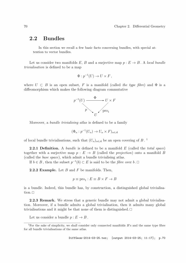
70 Chapter 2. Differential Geometry
2.2 Bundles
In this section we recall a few basic facts concerning bundles, with special at-tention to vector bundles.
Let us consider two manifolds E, B and a surjective map p : E → B . A local bundletrivialisation is defined to be a map
Φ : p−1(U)→ U × F ,
where U ⊂ B is an open subset, F is a manifold (called the type fibre) and Φ is adiffeomorphism which makes the following diagram commutative
p−1(U)Φ
- U × F
Upro1
p -
Moreover, a bundle trivialising atlas is defined to be a family
(Φα : p−1(Uα)→ Uα × F )α∈A
of local bundle trivialisations, such that (Uα)α∈A be an open covering of B . 1
2.2.1 Definition. A bundle is defined to be a manifold E (called the total space)together with a surjective map p : E → B (called the projection) onto a manifold B(called the base space), which admit a bundle trivialising atlas.
If b ∈ B , then the subset p−1(b) ⊂ E is said to be the fibre over b .
2.2.2 Example. Let B and F be manifolds. Then,
p ≡ pro1 : E ≡ B × F → B
is a bundle. Indeed, this bundle has, by construction, a distinguished global trivialisa-tion.
2.2.3 Remark. We stress that a generic bundle may not admit a global trivialisa-tion. Moreover, if a bundle admits a global trivialisation, then it admits many globaltrivialisations and it might be that none of them is distinguished.
Let us consider a bundle p : E → B .
1For the sake of simplicity, we shall consider only connected manifolds B’s and the same type fibrefor all bundle trivialisations of the same atlas.
DiffGeom-2014-03-25.tex; [output 2014-03-25; 11:17]; p.70

2.2. Bundles 71
2.2.4 Remark. Let A be a bundle trivialising atlas. A local manifold chart of thebase space and a local chart of the type fibre
(xλ) : U ⊂ B → IRm (yi) : F → IRl
yield a local manifold chart denoted by
(xλ, yi) : p−1(U)→ IRm × IRl
of E , which is said to be fibred.
We shall refer to a fibred manifold atlas (xλ, yi) .
A section is defined to be a map s : B → E , such that p s = idB . Thus, thecoordinate expression of the section s is of the type
(xλ, yi) s = (xλ, si) ,
where (si) : B → IRl .
2.2.5 Definition. The fibred product of the bundles p : E → B and p′ : E ′ → B overthe same base space B is defined to be the bundle whose total space is
E ×BE ′ :=
⊔b∈B
Eb × E ′b
and whose projection map is the natural projection
E ×BE ′ → B : (X, Y ) ∈ Eb × E ′b 7→ b .
2.2.6 Definition. A bundle morphism between two bundles p : E → B and p′ :E ′ → B′ is defined to be a map f : E → E ′ which preserves thefibres, i.e. such that thefollowing diagram commutes
Ef- E ′
B
p? f
- B′
p′?
where f : B → B′ is a map which turns out to be unique.We say that f is a bundle morphism over f . In the particular case when B = B′ and
f = idB , we say that f is a bundle morphism over B .
Let N be any manifold. We shall naturally identify the maps f : E → N with thebundle morphisms f : E → B ×N over B .
Next, we recall a few facts on vector bundles.
DiffGeom-2014-03-25.tex; [output 2014-03-25; 11:17]; p.71

72 Chapter 2. Differential Geometry
In the case when the fibres of the bundle are equipped with a vector structure, a localbundle trivialisation Φ : p−1(U) → U × F is said to be linear if the type fibre F is avector space and, for each b ∈ U , the map Φb : Eb → F is a linear isomorphism. Moreover,a bundle trivialising atlas is said to be linear if it is constituted by linear local bundletrivialisations.
2.2.7 Definition. A vector bundle is defined to be a bundle p : E → B togetherwith a vector structure on each fibre Eb, b ∈ B , which admits a linear bundle trivialisingatlas.
If p : E → B is a vector bundle, the bundle trivialising atlas is linear and the chart(yi) is linear, then also the induced manifold chart is said to be linear.
Let p : E → B be a vector bundle and Φ : p−1(U) → U × F a linear local bundletrivialisation. Then, an (fi) a basis of F and the dual basis (φi) of F ∗ yield the local basisof sections and the linear fibred chart
bi : U → p−1(U) : b 7→ Φ−1(b, fi) yi : p−1(U)→ IR : v 7→ φi(
pro2(φ(v))).
If p : E → B, p′ : E ′ → B′ are vector bundles, then a bundle morphism f : E → E ′ issaid to be linear if it restricts to linear maps between fibres.
2.2.8 Remark. Let p : E → B be a vector bundle. Then, the set
E∗ :=⊔b∈B
E∗b
constituted by the disjoint union of the dual spaces of the fibres of E turns out to benaturally a vector bundle over B .
Moreover, each linear fibred chart of E yields, by duality, a linear fibred chart of E∗ .
2.2.9 Remark. Let p : E → B, p′ : E ′ → B be vector bundles over the same basespace. Then, the set
E ⊗BE ′ :=
⊔b∈B
Eb ⊗ E ′b
constituted by the disjoint union of tensor products of the fibres of E and E ′ over thesame base points turns out to be naturally a vector bundle over B .
Moreover, each pair of linear fibred charts of E and E ′ yields, by tensor product, alinear fibred chart of E ⊗
BE ′ .
2.2.10 Remark. Let p : E → B be a vector bundle. Then, there is a natural bijection
s : B → E∗ 7→ f : E → IR
between the sections of the dual bundle and the linear fibred functions of the bundle.Accordingly, we shall identify the above objects.
DiffGeom-2014-03-25.tex; [output 2014-03-25; 11:17]; p.72
2.2. Bundles 73
2.2.11 Remark. Let p : E → B, p′ : E ′ → B be vector bundles over the same basespace. Then, there is a natural bijection
s : B → E∗ ⊗BE ′∗ 7→ f : E ⊗
BE ′ → IR
between the sections of the dual tensor product bundle and the linear fibred functions ofthe tensor product bundle. Accordingly, we shall identify the above objects.
Now, we introduce the concept of fibre metric of a vector bundle.
2.2.12 Definition. Let p : E → B be a vector bundle. Then, a fibred metric on E isdefined to be a section
g : B → E∗ ⊗BE∗
of the bundle E∗ ⊗BE∗ → B such that, for any b ∈ B , the tensor
gb ∈ E∗b ⊗ E∗b
corresponds to a positive definite symmetric bilinear map
gb : Eb × Eb → IR .
DiffGeom-2014-03-25.tex; [output 2014-03-25; 11:17]; p.73
74 Chapter 2. Differential Geometry
2.3 Tangent prolongation of manifolds
In this section we recall a few basic facts concerning the tangent prolongationof manifolds.
Let us consider a manifold M and a manifold atlas xλ : U → IRm .
Let c, c′ : IR → M be two local curves and t, t′ ∈ IR two real numbers. We define thefollowing equivalence relation
(t, c) ∼ (t′, c′) ⇔ c(t) = c′(t′), Dcλ(t) = Dc′λ(t′) ,
with respect to any manifold chart.
We denote the equivalence class of the couple (t, c) by
dc(t) ≡ [(t, c)] .
Let p ∈M be a point. We define the tangent space of M at p to be the set
TpM := dc(t)c(t)=p
constituted by all equivalence classes [(t, c)] such that c(t) = p .
2.3.1 Definition. The tangent space of M is defined to be the set
TM :=⊔p∈M
TpM .
2.3.2 Proposition. The natural projection.
τM : TM →M
is a vector bundle.
Proof. Clearly, TM turns out to be a manifold, as each manifold chart xλ : U → IRm yields thechart
(xλ, xλ) : τ−1(U)→ IRm × IRm : dc(t) 7→(cλ(t), Dcλ(t)
)and the transition maps of these charts are smooth.
Moreover, the map τ turns out to be smooth.
Furthermore, τ makes TM a bundle over M .
In fact, each manifold chart xλ : U → IRm yields the bundle trivialisation
τ−1(U)→ U × IRm : dc(t) 7→(c(t), Dcλ(t)
).
Indeed, different charts induce the same vector structure on the fibres of the tangent bundle. Hence,τ : TM →M turns out to be naturally a vector bundle. QED
DiffGeom-2014-03-25.tex; [output 2014-03-25; 11:17]; p.74

2.3. Tangent prolongation of manifolds 75
2.3.3 Remark. We say a manifold M to be parallelisable if TM admits a globaltrivialisation TM 'M × IRm .
In general, manifolds are not parallelisable. For example, it can be proved that theunit sphere S2 ⊂ IR3 is not parallelisable.
Anyway, we have a distinguished class of parallelisable manifolds: affine spaces asso-ciated with vector spaces.
Namely, if P is an affine space associated with a vector space DP , then we obtain anatural isomorphism induced by any affine global chart of P
TP ' P ×DP ,
by which we will identify the above spaces.In particular, by regarding DP as an affine space associated with DP , then
TDP = DP ×DP .
A section X : M → TM is said to be a vector field.If c : IR→M is a curve, then its tangent prolongation is defined to be the curve
dc : IR→ TM : t→ dc(t) .
By construction, we have the following coordinate expression
(xλ, xλ) dc = (cλ, Dcλ) .
2.3.4 Example. Let P be an affine space and c : IR→ P a curve. Then, we can write
dc = (c, Dc) : IR→ TP = P ×DP .
Let us consider a family of curves parametrised by a manifold N
φ : IR×N →M .
Then, we define the variational differential of f as
∂φ : N → TM : q 7→ d(φq)(0) .
In particular, the tangent prolongation of the coordinate curves xα : IR×M →M arethe vector fields
∂xα : M → TM : p 7→ d(xαp)(0) .
Let f : M → IR be a function. Then, we define the α-th partial derivative of f , withrespect to the coordinate curve xα , to be the function
∂αf ≡ ∂xα.f : M → IR : p 7→ ∂(f xα) :=D(f xαp)(0) .
DiffGeom-2014-03-25.tex; [output 2014-03-25; 11:17]; p.75

76 Chapter 2. Differential Geometry
The standard notation for the partial derivative is
∂f
∂xα: M → IR ;
however, we prefer the above notation, because the partial derivative depends on the α-thcoordinate curve xα and not on the α-th coordinate function xα . Moreover, we shall seesoon a natural interpretation of our notation.
2.3.5 Proposition. If f : M →M ′ is a map, then there is a unique map
Tf : TM → TM ′ ,
such that the following diagram commutes, for each curve c : IR→M ,
TMTf
- TM ′
IRd(f c)
-
dc
Moreover, Tf is a linear fibred morphism over f , hence the following diagram com-mutes
TMTf−−−→ TM ′
τM
y yτ ′MM −−−→
fM ′
2.3.6 Example. Let P, P ′ be affine spaces and f : P → P ′ a map. Then, we canwrite
Tf = (f ×Df) : TP = P ×DP → TP ′ = P ′ ×DP ′ .
2.3.7 Definition. We define the cotangent bundle to be the dual bundle of the tan-gent bundle
τM : T ∗M →M .
The natural fibred chart of T ∗M will be denoted by
(xα, xα) .
2.3.8 Remark. Let M be a manifold, P an affine space and f : M → P a map.Then, we define the differential of f to be the fibred linear map
f = pro2 Tf : TM → DP ,
or, equivalently, the corresponding section
df : M → T ∗M .
DiffGeom-2014-03-25.tex; [output 2014-03-25; 11:17]; p.76

2.3. Tangent prolongation of manifolds 77
In particular, if f : M → IR is a function, then we obtain
f : TM → IR df : M → T ∗M ⊗DP .
This notation agrees with the notation we have already adopted for affine spaces andcoordinate functions on the tangent space.
2.3.9 Example. Let P be an affine space and f : P → IR a function. Then, we have
f : P ×DP → IR : (a, h) 7→ Dfa(h)
df : P → P ×D∗P : a 7→ (a, Dfa) .
2.3.10 Remark. The differentials of the coordinate functions are the fibred linearmaps
xλ = pro2 Txλ : TM → IR ,
or equivalently the sections
dxλ : M → T ∗M .
2.3.11 Lemma. For each p ∈ M , the m vectors ∂xα(p) and the m forms dxα con-stitute a basis of TpM and the dual basis of T ∗pM .
Proof. In fact, by differentiating the equality
(xα xβ)(t, p) = xα(p) + δαβ t ,
we obtain
∂(xα xβ) = δαβ ,
which yields the claim in virtue of a well known result of linear algebra. QED
2.3.12 Theorem. Let f : M → N be a map. Then, the coordinate expression of Tfis
(x′λ, x′λ) Tf = (f ′λ,∂f ′λ
∂xµxµ) .
In other words, by regarding Tf as a section
Tf : M → T ∗M ⊗ TN ,
we can write
Tf = ∂xµ.f′λdxµ ⊗ ∂(x′λ f) .
Proof. The results follows immediately from the chain rule and the definition of partial derivative.In fact, we can write
(Tf ′)λµ = 〈dx′λ, T f(∂xµ)〉 = ∂(x′λ f xµ) := ∂xµ.f′λ .QED
DiffGeom-2014-03-25.tex; [output 2014-03-25; 11:17]; p.77

78 Chapter 2. Differential Geometry
2.3.13 Corollary. The coordinate expressions of the tangent prolongation of a curvec : IR→M and of a function f : M → IR are
dc = Dcλ(∂xλ c)df = ∂λfdx
λ .
2.3.14 Remark. The vector subspace
F(M) := f : M → IR | fsmooth ⊂ M(M, IR)
is endowed by the operations inM(M, IR) with the structure of a commutative associativealgebra with unity.
2.3.15 Proposition. A vector field X : M → TM yields a derivation of F(M) , i.e.a linear map
X. : F(M)→ F(M) : f 7→ X.f := 〈df, X〉 ,with the property, for each f, f ′ ∈ F(M) ,
X.(ff ′) = fX.f ′ + f ′X.f .
We have the coordinate expression
X.f = Xλ∂xλ.f .
2.3.16 Remark. The above notation fits our notation for partial derivatives. In fact,we can write
∂xλ.f = 〈df, ∂xλ〉 .
Conversely, one can prove that vector fields are characterised by their action on func-tions.
2.3.17 Proposition. If δ : F(M) → F(M) is a derivation, then there is a uniquevector field X : M → TM such that, for each f ∈ F(M) ,
X.f = δ(f) .
We can use the above fact in order to introduce the commutator of two vector fields.
2.3.18 Remark. If X, Y : M → TM are vector fields, then the map X.Y. : F(M)→F(M) is not a derivation of F(M) , hence cannot be identified with a vector field. In fact,we have the following coordinate expression
X.Y.f = Xλ∂λYµ∂µf +XλY µ∂λµf .
However, we have the following result.
DiffGeom-2014-03-25.tex; [output 2014-03-25; 11:17]; p.78
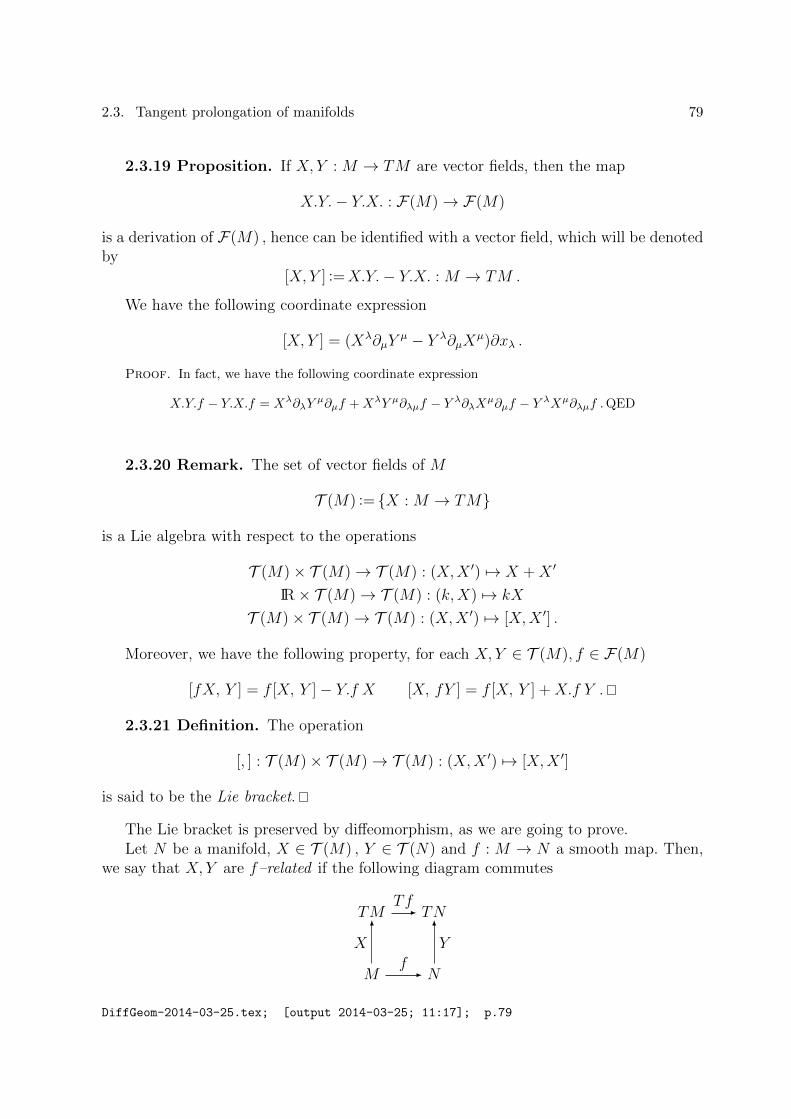
2.3. Tangent prolongation of manifolds 79
2.3.19 Proposition. If X, Y : M → TM are vector fields, then the map
X.Y.− Y.X. : F(M)→ F(M)
is a derivation of F(M) , hence can be identified with a vector field, which will be denotedby
[X, Y ] :=X.Y.− Y.X. : M → TM .
We have the following coordinate expression
[X, Y ] = (Xλ∂µYµ − Y λ∂µX
µ)∂xλ .
Proof. In fact, we have the following coordinate expression
X.Y.f − Y.X.f = Xλ∂λYµ∂µf +XλY µ∂λµf − Y λ∂λXµ∂µf − Y λXµ∂λµf .QED
2.3.20 Remark. The set of vector fields of M
T (M) := X : M → TM
is a Lie algebra with respect to the operations
T (M)× T (M)→ T (M) : (X,X ′) 7→ X +X ′
IR× T (M)→ T (M) : (k,X) 7→ kX
T (M)× T (M)→ T (M) : (X,X ′) 7→ [X,X ′] .
Moreover, we have the following property, for each X, Y ∈ T (M), f ∈ F(M)
[fX, Y ] = f [X, Y ]− Y.f X [X, fY ] = f [X, Y ] +X.f Y .
2.3.21 Definition. The operation
[, ] : T (M)× T (M)→ T (M) : (X,X ′) 7→ [X,X ′]
is said to be the Lie bracket.
The Lie bracket is preserved by diffeomorphism, as we are going to prove.Let N be a manifold, X ∈ T (M) , Y ∈ T (N) and f : M → N a smooth map. Then,
we say that X, Y are f–related if the following diagram commutes
TMTf- TN
M
X6
f- N
Y6
DiffGeom-2014-03-25.tex; [output 2014-03-25; 11:17]; p.79

80 Chapter 2. Differential Geometry
2.3.22 Proposition. Let N be a manifold, X,X ′ ∈ T (M) , Y, Y ′ ∈ T (N) and f :M → N a smooth map. Suppose that X, Y and X ′, Y ′ are f–related.
Then, [X,X ′] is f–related to [Y, Y ′] .
Let f : M → N be a diffeomorphism, and X ∈ T (M) .Let us set f∗X :=Tf X f−1 ∈ T (N) . Then, f∗X is the unique vector field on N
being f–related to X .
2.3.23 Corollary. Let f : M → N be a diffeomorphism, and X,X ′ ∈ T (M) . Then,
f∗[X,X′] = [f∗X, f∗X
′] .
DiffGeom-2014-03-25.tex; [output 2014-03-25; 11:17]; p.80

2.4. Tangent prolongation of bundles 81
2.4 Tangent prolongation of bundles
In this section we recall a few basic facts concerning the tangent prolongationof bundles.
So, we go back to a generic bundle p : E → B and apply the constructions ofthe above section to it.
2.4.1 Remark. The set TE is naturally a manifold equipped with the manifold atlas
(xλ, yi; xλ, yi) .
Moreover, τE : TE → E turns out to be naturally a vector bundle. We have thecoordinate expression
(xλ, yi) τE = (xλ, yi) .
Furthermore, we have the linear bundle morphism
Tp : TE → TB ,
over p : E → B , with coordinate expression
(xλ, xλ) Tp = (xλ, xλ) .
Thus, the following diagram commutes
TETp−−−→ TB
τE
y yτBE −−−→
pB
2.4.2 Remark. We can see that, if p : E → B is a vector bundle with type fibre F ,then also Tp : TE → TB is a vector bundle with type fibre TF = F × F .
2.4.3 Remark. We can easily see that a vector X ∈ TeE is tangent to the fibre Ep(e)passing through its base point e ∈ E if and only if Tp(X) = 0 . Such vectors are said tobe vertical. The subset of vertical vectors constitutes a vector subbundle
ι : V E → TE
over E , which is characterised by the system of equations
xλ = 0
and called the vertical bundle.In particular, if p : E → B is a vector bundle, then we can write
V E = E ×BE ,
DiffGeom-2014-03-25.tex; [output 2014-03-25; 11:17]; p.81
82 Chapter 2. Differential Geometry
because we know that the tangent space of a vector space is the product of the vectorspace times itself.
As a special case, we can apply the above constructions to the tangent bundle of themanifold M
p ≡ τ : E ≡ TM → B ≡M .
In this case we obtain some interesting identifications.
2.4.4 Example. We denote the induced local chart of TTM by
(xλ, xλ; xλ, xλ) .
We have two vector bundle projections
τTM : TTM → TM TτM : TTM → TM ,
with coordinate expressions
(xλ, xλ) τTM = (xλ, xλ) (xλ, xλ) TτM = (xλ, xλ) .
We haveV TM = TM ×
MTM .
DiffGeom-2014-03-25.tex; [output 2014-03-25; 11:17]; p.82

2.5. Connections on bundles 83
2.5 Connections on bundles
In this section we introduce the concept of connection, with special attention tolinear connections on vector bundles.
Let us consider a bundle p : E → B and a fibred manifold atlas (xλ, yi) .
2.5.1 Remark. We have the following situation.
- Given a vector X ∈ TbB , and a point e ∈ Eb , we can prolong it to a vector X ∈ TeE ,which projects onto X , in many ways; but no distinguished prolongation exists.
- Given a vector X ∈ TeE , we can project it onto the vector Tp(X) ∈ Tp(e)B of thebase space B , hence we are able to say whether it is vertical or not. However, if X isnot vertical, then we can project it to a vertical vector Y ∈ VeE in many ways; but nodistinguished projection exists.
- We can easily see that the two missing operations are equivalent.
- In other words, for each e ∈ Eb , we have several splittings
TeE ' TbB × VeE,
which fit the natural projection TeE → TbB and the natural inclusion VeE → TeE , butnone of them is distinguished.
So, in order to avail of such a distinguished splitting, we must postulate it by intro-ducing a new concept, which will be discussed in next section.
2.5.2 Definition. A connection is defined to be a linear splitting over E
TE ' (E ×BTB)×
EV E,
provided by
- the linear bundle morphism over E
γ : E ×BTB → TE ,
such that the composition
E ×BTB
γ- TE
(τE, Tp)- E ×BTB
is the identity map of E ×BTB ,
or, equivalently, by
- the linear bundle morphism over E
ν : TE → V E ,
DiffGeom-2014-03-25.tex; [output 2014-03-25; 11:17]; p.83

84 Chapter 2. Differential Geometry
such that the composition
V EιE - TE
ν- V E
is the identity map of V E .The map γ is called the horizontal prolongation and the map ν is called the vertical
projection.
Let us consider a connection γ or, equivalently, ν .
2.5.3 Proposition. If X : B → TB is a vector field of the base space, then itshorizontal prolongation is the vector field
γ(X) : E → TE ,
with coordinate expressions
γ(X)λ = Xλ and γ(X)i = γiλXλ;
if X : E → TE is a vector field of the total space, then its vertical projection is the vectorfield
ν(X) : E → V E ,
with coordinate expressions
ν(X)λ = 0 and ν(X)i = X i − γiλXλ,
where
(γiλ) : E → IRl × IRm
is a matrix, which characterises locally the connection.
2.5.4 Remark. Let s : B → E be a section. The natural differential of s is its tangentprolongation
Ts : TB → TE ,
with coordinate expression
(Ts)λ = xλ and (Ts)i = ∂λsixλ .
The information carried by the section s is encoded just in its components si andanalogously, the information carried by the differential Ts of the section is encoded justin its components (Tsi) . So, one can be interested in a distinguished vertical projection ofTs , which would be tangent to the fibres and would have as many significant componentsas the section s itself: this is provided by the connection γ .
So, we are led to introduce the following concept.
DiffGeom-2014-03-25.tex; [output 2014-03-25; 11:17]; p.84
2.5. Connections on bundles 85
2.5.5 Definition. Let s : B → E be a section and X : B → TB a vector field of thebase space. The covariant differential of s is defined to be the map
∇Xs := ν Ts X : B → V E .
2.5.6 Remark. Of course, we have
τE ∇Xs = s .
2.5.7 Remark. Let s : B → E be a section and X,X ′ : B → TB vector fields. Thecovariant derivative fulfills the property
∇X+X′s = ∇Xs+∇′Xs .
We have the coordinate expression
(∇Xs)i = (∂λs
i − γiλ s)Xλ .
Next, let us assume that p : E → B is a vector bundle and let us refer to a linearfibred atlas.
2.5.8 Remark. Let us recall that we can write V E = E ×BE . Accordingly, the first
component of the covariant derivative ∇Xs is just s itself. Therefore, in order to simplifythe notation we shall omit, by abuse of language, the first component of the verticalprojection and of the covariant derivative and keep only the second components; hence,we write
ν : TE → E and ∇Xs : B → E .
We recall that Tp : TE → TB is a vector bundle.
2.5.9 Definition. The connection γ is said to be linear if γ , regarded as a bundlemorphism over TB , is linear.
2.5.10 Proposition. The connection γ is linear if and only if its coordinate expressionis of the type
γiλ = γiλjyj ,
where(γiλj) : B → IRm × IRl × IRl .
Let us suppose that the connection γ be linear.
2.5.11 Proposition. Let s, s′ : B → E be sections, f : B → IR a function andX : B → TB a vector field. Then, the covariant derivative fulfills the properties
∇X(s+ s′) = ∇Xs+∇Xs′ and ∇X(fs) = X.fs+ f∇Xs .
DiffGeom-2014-03-25.tex; [output 2014-03-25; 11:17]; p.85
86 Chapter 2. Differential Geometry
We have the coordinate expression
(∇Xs)i = (∂λs
i − γiλjsj)Xλ .
2.5.12 Proposition. Conversely, let us assume to have defined a law ∇ which mapseach local section s : B → E and local vector field X : B → TB onto a local section
∇Xs : B → E ,
with the properties
∇X+X′s = ∇Xs+∇′Xs ,∇X(s+ s′) = ∇Xs+∇Xs
′ , ∇X(fs) = X.fs+ f∇Xs
and which commutes with local restrictions.Then, there exist a unique linear connection γ which yields the above law.
Next, we introduce the concept of metrical connection.
2.5.13 Definition. Let us assume a fibred metric on the bundle p : E → B
g : B → E∗ ⊗BE∗ .
The linear connection γ is said to be metric if, for any section s, s′ : B → E andvector field X : B → TB , we have
X.(g (s, s′)
)= g (∇Xs, s
′) + g (s,∇Xs′) .
DiffGeom-2014-03-25.tex; [output 2014-03-25; 11:17]; p.86

2.6. Connections on manifolds 87
2.6 Connections on manifolds
In this section we apply the above constructions on linear connections to thetangent bundle τM : TM →M of a manifold M , with special attention to Rieman-nian connections on Riemannian manifolds.
2.6.1 Remark. A linear connection on the vector bundle τM : TM → M can beregarded, equivalently, as the horizontal prolongation
γ : TM ×MTM → TTM ,
or as the vertical projectionν : TTM → TM .
The coordinate expression of the connection is of the type
γαλ = γαλµxµ .
The covariant derivative of a vector field Y : M → TM , with respect to a vector fieldX : M → TM , is the vector field
∇XY : M → TM ,
with coordinate expression
(∇XY )α = (∂λYα − γαλµY µ)Xλ .
Thus, we can writeγαλµx
µ = −(∇∂xλ∂xµ)α .
2.6.2 Remark. Let c : IR→M be a curve and ν : TTM → TM a linear connection.We know that the tangent prolongation of c is the curve
dc : IR→ TM .
Moreover, by iterating the tangent prolongation, we obtain the second tangent pro-longation of c , which is the curve
d2c : IR→ TTM ,
with coordinate expression
(xλ, xλ; xλ, xλ) d2c = (cλ, Dcλ, Dcλ, D2cλ) .
Thus, d2c is a natural second derivative that we can perform on c by taking intoaccount only the differentiable structure of M . But, this map has some disadvantages:
DiffGeom-2014-03-25.tex; [output 2014-03-25; 11:17]; p.87
88 Chapter 2. Differential Geometry
- it has values in TTM , while it might be desirable it had values in the same spaceof the first tangent prolongation, namely in TM ;
- its coordinate expression carries a reduntant information, as the first derivatives Dcλ
are repeated twice.These, problems can be easily overcome by taking into account the connection and
introducing the map
∇dc := ν D2c : IR→ TM ,
with coordinate expression
∇dc =(D2cλ − (γλµν c)DcµDcν
)∂xλ c .
We can relate the above map with the standard covariant derivative in this way. LetX : M → TM be any extension of dc , i.e. any vector field such that X c = dc . Then,by a simple computation in coordinates we can prove that
(∇XX) c = ∇dc .
2.6.3 Example. Let M be a parallelisable manifold. Then, the choice of a bundleisomorphism TM →M × IRm yields the bundle isomorphism
TTM →M × IRm × IRm × IRm ,
which restricts to the bundle isomorphism
V TM →M × IRm × 0 × IRm .
Hence, we have the connection
pro : TTM → V TM : (x, v, v′, w) 7→ (x, v, 0, w) ,
and, if c : IR→M , then
∇dc := pro D2c
with γλµν = 0 .If M is an affine space associated with the vector space DM , then the affine structure
induces a distinguished bundle isomorphism TM →M ×DM . Hence, as before, we havea distinguished connection on M which is induced by the affine structure.
2.6.4 Proposition. Let γ be a linear connection of the vector bundle τM : TM →M .The map
τ : (X, Y ) 7→ ∇XY −∇YX − [X, Y ]
is bilinear, hence can be regarded as a bilinear fibred morphism over M
τ : TM ×MTM → TM .
DiffGeom-2014-03-25.tex; [output 2014-03-25; 11:17]; p.88

2.6. Connections on manifolds 89
Its coordinate expression is
ταλµ = −γαλµ + γαµλ .
Proof. If f : M → IR is a function, then we have
τ(fX, Y ) = f(∇XY −∇YX − [X,Y ])− (Y.f)X + (Y.f)X = τ(fX, Y )
τ(X, fY ) = f(∇XY −∇YX − [X,Y ]) + (X.f)Y − (X.f)Y = τ(X, fY ) .
Moreover, we have
ταλµ = (∇∂xλxµ −∇∂xµxλ)α .QED
The map τ is said to be the torsion of the linear connection γ . Moreover, if τ vanishes,then γ is said to be torsion free.
Of course, the linear connection γ is torsion free if and only if its coordinate expressionis symmetric in the two subscripts λ and µ with respect to any chart.
2.6.5 Definition. A linear connection on the manifold M is defined to be a lineartorsion free connection on the vector bundle τM : TM →M .
2.6.6 Definition. A Riemannian metric g on the manifold M is defined to be afibred metric on TM , i.e.
g : M → T ∗M ⊗MT ∗M → IR .
A manifold M , together with a Riemannian metric g , is said to be a Riemannianmanifold.
Let us consider a Riemannian manifold (M, g) .The coordinate expression of g is
g = gλµ dxλ ⊗ dxµ .
2.6.7 Theorem (Levi-Civita). There is a unique metric torsion free linear connectionκ on the Riemannian manifold (M, g) . More precisely, the coordinate expression of κ is
καλµ = −1
2gαβ(∂λgβµ + ∂µgβλ − ∂βgλµ) .
Proof. The metricity condition implies
∂βgλµ = −gαµκαβλ − gαλκαβµ
i.e.
∂βgλµ = −κβµλ − κβλµ .
DiffGeom-2014-03-25.tex; [output 2014-03-25; 11:17]; p.89

90 Chapter 2. Differential Geometry
Moreover, by circular permutation of the subscripts in the above formula, we obtain
∂µgβλ = −κλβµ − κµβλ∂βgλµ = −κλβµ − κµβλ .
Eventually, we obtain the result by subtracting the above two equalities from the previous one andby taking into account the symmetry of the symbols of the connection. QED
DiffGeom-2014-03-25.tex; [output 2014-03-25; 11:17]; p.90
2.7. Lie Groups 91
2.7 Lie Groups
In this section we recall some basic fact from the theory of Lie groups.
Moreover, we will deal with some distinguished examples which will play animportant role in the second part of the book.
2.7.1 Lie Groups
Here, we recall the definition and the main properties of Lie groups. Some ofthe deepest result of the theory of Lie groups will only be stated. The interestedreader can go through details of proofs in the bibliographical references.
2.7.1 Definition. A Lie group is defined to be a group G endowed with a manifoldstructure such that the maps
l : G×G→ G : (g, g′) 7→ gg′ , i : G→ G : g 7→ g−1 ,
are smooth.
2.7.2 Remark. Let G be a Lie group. Then, for each g ∈ G , the restriction of themultiplication
lg : G→ G : h 7→ gh
is a diffeomorphism of G with itself, which is said to be the left translation by g .
Left translation provide a distinguished global trivialisation of TG , as we are goingto see.
2.7.3 Definition. We say a vector field X : G → TG on a lie group G to be leftinvariant if for each g ∈ G we have lg∗X = X .
We denote by g the set of left invariant vector fields on G .
In virtue of corollary 2.3.23, g ⊂ T (G) is a Lie subalgebra. We say g to be the Liealgebra of the Lie group G.
2.7.4 Proposition. There is a natural isomorphism
g→ T1GG : X 7→ X1G .
Proof. We can extend any v ∈ T1GG to a vector field Xv : G→ TG by the formula
Xv : G→ TG : g 7→ T lg(X) ;
of course, we have Xv(1G) = v . This ensures both injectivity and surjectivity of the linear map of thestatement. QED
DiffGeom-2014-03-25.tex; [output 2014-03-25; 11:17]; p.91

92 Chapter 2. Differential Geometry
Of course, g is a finite dimensional vector space; namely, dim g = dimT1GG = dimG .We have the tensor representation [, ] = V ∗ ⊗ V ∗ ⊗ V , and, if (ei) is a basis of g , thenwe have the matrix representation
[, ] = ckijεi ⊗ εj ⊗ ek .
The real numbers ckij are said to be the structure constants of G with respect to (ei) .
2.7.5 Proposition. If G is a Lie group, then we have the natural linear bundleisomorphism over G
G× g→ TG : (g,X) 7→ X(g) ,
by which we identify the above spaces.
2.7.6 Remark. Each Lie group G admits a natural parallelisation. Hence, thefollow-ing consequences hold in a straightforward way.
1. A non parallelisable manifold M cannot be endowed with the structure of a Liegroup.
2. G is orientable.
3. G is endowed with the natural connection induced by the distinguished parallelisa-tion (remark 2.6.3).
Let G,H be Lie groups. Then f : G → H is said to be a Lie group morphism if f isa smooth group morphism. The following straightforward property holds.
2.7.7 Proposition. Let G,H be Lie groups with Lie algebras g, h , and f : G → Ha Lie group morphism. Then, f induces a Lie algebra morphism
g→ h : X 7→ YX
where YX(1H) = T1Gf(X1G) .
2.7.8 Definition. Let G be a Lie group, and H ⊂ G . Then, H is said to be a Liesubgroup of G if H is a subgroup and a submanifold of G .
2.7.9 Remark. A remarkable example of Lie subgroup of a Lie group G is providedby the connected component G1G of G containing 1G . The other connected componentsare diffeomorphic to G1G by left translations.
2.7.10 Theorem. Let G be a Lie group. Then, there is a bijective correspondencebetween connected Lie subgroups of G and Lie subalgebras of the Lie algebra g of G .—END
2.7.11 Theorem. Let G be a Lie group, and H a Lie subgroup. Then, H is anembedded submanifold of G if and only if H is closed.
DiffGeom-2014-03-25.tex; [output 2014-03-25; 11:17]; p.92

2.7. Lie Groups 93
2.7.12 Theorem. Let G be a Lie group, and H ⊂ G . Suppose that H be a closedset and a subgroup of G . Then, H has a unique manifold structure which makes H a Liesubgroup of G .
Moreover, as a consequence of the above theorem, with respect to this manifold struc-ture H is an embedded submanifold of G .
Given a Lie group G , we can consider the quotient G/H with a closed subgroupH ⊂ G . If H is a normal subgroup of G , then the group structure of G passes to thequotient, endowing G/H with a natural group structure. But, even if H is not normal,we are able to give a manifold structure on G/H .
2.7.13 Theorem. Let G be a Lie group, and H a closed subgroup. Denote by pro :G→ G/H the natural projection. Then, G/H has a unique manifold structure such thatpro : G→ G/H is a bundle.
Moreover, if H is normal, then the manifold G/H with its natural quotient groupstructure is a Lie group.
A manifold of the above type G/H is said to be a homogeneous manifold. It has to beremarked that several concrete examples of manifold are homogeneous manifolds.
Let G be a Lie group, and M a manifold. Then, a (left) action of G on M is a smoothmap
a : G×M →M
which is an action of the group G on the set M .Suppose that a be a transitive action, and m ∈M . Then, the isotropy subgroup Hm
(see remark 1.6.2) is a closed subgroup of G , hence a Lie subgroup.
2.7.14 Proposition. Let G be a Lie group, M a manifold and a : G ×M → M atransitive action. Let m ∈M , and consider the map
[am] : G/Hm →M : [g] 7→ a(g,m) .
Then, [am] is a diffeomorphism.
2.7.2 Affine spaces associated with Lie groups
Let C be an affine space associated with a Lie group DC . In this subsection, weshow that C can be endowed with the structure of a manifold which is diffeomorphicto DC .
2.7.15 Proposition. There exists a unique differentiable structure on C such that,for each o ∈ C , the map lo : DC → C is smooth.
Proof. For each o ∈ C , the bijection lo : DC → C makes C a smooth manifold. Moreover, ifo′ ∈ C , then lo and lo′ yield the same smooth structure on C , because the transition map, given byfollowing composition
δo′ lo : DC → DC : g 7→ (go)o′−1 ≡ g(oo′−1)
DiffGeom-2014-03-25.tex; [output 2014-03-25; 11:17]; p.93
94 Chapter 2. Differential Geometry
is the left translation loo′−1 : DC → DC , which is smooth. QED
It turns out that for any o ∈ C the map δo : C → DC is smooth.
2.7.16 Proposition. Let Dc be the Lie algebra of DC . Then, we have the naturalisomorphism
TC ' C × g .
by which we identify the above spaces.
Proof. Let o ∈ C . Then, by using the natural parallelisation TDC ' DC ×Dc
(lo, idDc) Tδo : TC → C ×Dc
is a parallelisation, and is independent from the choice of o .QED
2.7.17 Corollary. The affine space C associated with the Lie group DC is orientableand is endowed with a natural connection associated with the natural parallelisation(remark 2.6.3).
2.7.3 Automorphisms of a vector space
Let V be a finite dimensional vector space, with dimV = n . We study the groupAut(V ) . Namely, we prove that Aut(V ) is a Lie group, and study its Lie algebra.Finally, we study some of its subgroup.
2.7.18 Lemma. The vector space V , regarded as an abelian group with respect tothe sum of vectors, has a natural structure of Lie group. The Lie algebra of V turns outto be naturally isomorphic to V itself.
2.7.19 Proposition. The group Aut(V ) is a Lie group with respect to the composi-tion of maps.
The Lie algebra of Aut(V ) is End(V ) endowed with the commutator.
Proof. The group Aut(V ) is an open subset of the vector space End(V ) , namely Aut(V ) =det−1(IR \ 0) (see definition 1.5.5). Hence, Aut(V ) is a manifold and
TidV Aut(V ) ≡ TidV End(V ) ' End(V ) ,
where the last map is the restriction of the natural parallelisation of End(V ) .The matrix representation of the composition of maps is smooth, hence Aut(V ) is a Lie group.Let (bi) be a basis of V . Then, the matrix representation induces the vector space isomorphism
End(V )→Mnn and the group isomorphism Aut(V )→ Inn , where Inn are the invertible matrices.
A left invariant vector field X on Inn is of the type
X : Inn → TInn : (aij) 7→ aikxkj∂i
j ,
with xij∂ij ∈ Mn
n . If Y is another left invariant vector field generated by yij∂ij ∈ Mn
n , then we seethat
[X,Y ](aij) = aik(xkjyjh − ykjxjh)∂i
h ,
DiffGeom-2014-03-25.tex; [output 2014-03-25; 11:17]; p.94

2.7. Lie Groups 95
hence [X,Y ](δij) = (xkjyjh − ykjx
jh)∂k
h . This is the matrix representation of the commutator inEnd(V ) .QED
2.7.20 Proposition. The Lie group Aut(V ) has two connected components. Thegroup
SAut(V ) ⊂ Aut(V )
is the connected component of Aut(V ) containing idV .Hence, SAut(V ) is a Lie subgroup of Aut(V ) having the same Lie algebra.
From now on, we assume a metric g on V .
2.7.21 Proposition. The subgroup O(V ) is a Lie subgroup of Aut(V ) .The Lie algebra of O(V ) is the following Lie subalgebra so(V ) of End(V )
so(V ) := f ∈ End(V ) | g(f(v), w) + g(v, f(w)) = 0 ∀v, w ∈ V .
Proof. In fact, O(V ) is a closed subgroup of Aut(V ) .Let us consider a smooth curve c : IR → O(V ) such that c(0) = id . If v, w ∈ V , by differentiating
the identity g(c(t)(v), c(t)(w)) = g(v, w) in 0 we obtain the identity
g(Dc(0)(v), w) + g(v,Dc(0)(w)) = 0 .QED
2.7.22 Proposition. The Lie group O(V ) has two connected components. The group
SO(V ) ⊂ O(V )
is the connected component of O(V ) containing idV .Hence, SO(V ) is a Lie subgroup of O(V ) having the same Lie algebra.
2.7.23 Remark. If dimV = 1 , then O(V ) ≡ ± id .If dimV = 2 , then an orthonormal basis yields an isomorphism of SO(V ) with the
unit sphere S1 ⊂ IR2 .
There is a natural action of O(V ) on V , namely
O(V )× V → V : (f, v) 7→ f(v) .
Let us setSV := v ∈ V | g(v, v) = 1 ;
the choice of an orthonormal basis of V yields a diffeomorphism SV → Sn−1 ⊂ IRn , henceSV is a manifold.
2.7.24 Lemma. The above natural action of O(V ) on V restricts to a transitiveaction
O(V )× SV → SV : (f, v) 7→ f(v) .
DiffGeom-2014-03-25.tex; [output 2014-03-25; 11:17]; p.95

96 Chapter 2. Differential Geometry
2.7.25 Proposition. Let v ∈ SV , and let us set v⊥ := span(v)⊥ .Then, the isotropy group of the above transitive action of O(V ) on SV at v is isomor-
phic to the set of orthogonal maps O(v⊥) of the Euclidean space (v⊥, g⊥) .Hence, we have the diffeomorphism
O(V )/O(v⊥)→ SV : [f ] 7→ f(v) .
Proof. It is easily proved in coordinates adapted to the splitting V = span(v) ⊕ v⊥ . The laststatement comes from proposition 2.7.14. QED
2.7.26 Remark. Analogous considerations hold for SO(V ):given v ∈ V , we have the natural diffeomorphism
SO(V )/SO(v⊥)→ SV : [f ] 7→ f(v) .
We end this subsection by showing that the group of rigid transformations of an affinespace associated with a Euclidean space can be endowed with the structure of a Lie group.
2.7.27 Proposition. Let P be an affine space associated with the Euclidean space(V, g) . Then, the group R(P ) can be endowed with a unique Lie group structure suchthat the natural isomorphism
R(P )→ DP ×O(DP, g) : f 7→ (τf(p), Df)
is a Lie group isomorphism for any p ∈ P .
Proof. In fact, the choice of p ∈ P yields a group isomorphism which endows R(P ) with thestructure of a Lie group. Then, it is easy to see that this structure does not depend on the choice ofp .QED
DiffGeom-2014-03-25.tex; [output 2014-03-25; 11:17]; p.96