notes on differential geometry part 1. geometry of curves

NOTES ON DIFFERENTIAL GEOMETRY

MICHAEL GARLAND

Part 1. Geometry of Curves

We assume that we are given a parametric space curve of the form

(1) x(u) =

x1(u)x2(u)x3(u)

u0 ≤ u ≤ u1

and that the following derivatives exist and are continuous

(2) x′(u) =dxdu

x′′(u) =d2xdu2

1. Arc Length

The total arc length of the curve from its starting point x(u0) to somepoint x(u) on the curve is defined to be

(3) s(u) =∫ u

u0

√x′ ·x′ du

It is also common to express this equation in a differential form:

(4) ds2 = dx·dx

The differential ds is referred to as the element of arc of the curve.Because we know that ds/du 6= 0, it is always permissible to reparame-

terize the curve x(u) in terms of its arc length x(s). This reparameterizedcurve has derivatives:

(5) x(s) =dxds

x(s) =d2xds2

Such a parameterization of the curve is often called a unit-speed parameter-ization because ‖x‖ = 1.

Date: August 30, 2004.Copyright (c) 2003–2004 Michael Garland. All rights reserved.

1

2 MICHAEL GARLAND

r

P

Q

R

Figure 1. Local geometry around a point P . Points Q andR are equidistant from P along the curve.

2. Local Frames and Curvature

To proceed further, we need to more precisely characterize the local ge-ometry of a curve in the neighborhood of some point. All the necessaryproperties of the curve can be derived algebraicly, as with the definition ofarc length. However, before examining these algebraic definitions, let usconsider a more direction construction that will provide greater intuitionabout the geometry of the curve.

2.1. Geometric Construction. Consider a point P on the curve, withadditional points Q and R equidistant from P in opposite directions alongthe curve (see Figure 1). We can define a unique circle C passing throughthese points.

Now consider the circle C in the limit as Q and R approach P . This iscalled the osculating circle of the curve at P . It will pass through the pointP , thus touching the curve at this point. The tangent line of C at P willalso be the tangent line of the curve at P . Furthermore, the vector from Pto the origin of C is obviously perpendicular to the tangent line at P , andis therefore a normal vector of the curve at this point. The circle C also hassome radius ρ. We define the curvature at the point P to be κ = 1/ρ.

2.2. Algebraic Definitions. We assume that we are given a unit-speedparameterization (§1) of a curve x(s). The unit tangent vector t is simply

NOTES ON DIFFERENTIAL GEOMETRY 3

the first derivative of x:

(6) t = dx/ds = x

Note that this is a unit vector precisely because we have assumed that theparameterization of the curve is unit-speed. The second derivative x will beorthogonal to t, and thus defines a normal vector. The length of x will bethe curvature κ. Therefore, we can define both the curvature normal k andthe unit normal n as:

(7) k = dt/ds = x = κn

Since we are typically interested in curves embedded in E3, we can alsodefine the unit bi-normal

(8) b = t×n

For curves embedded in E3, these three unit vectors provide a completeorthonormal basis. They are often referred to collectively as the moving orlocal trihedron.

From the three vectors of the local trihedron, we can also define threecanonical planes through the point x

Normal plane: (y − x)·t = 0(9)

Rectifying plane: (y − x)·n = 0(10)

Osculating plane: (y − x)·b = 0(11)

It is the osculating plane that is usually of most interest to us, as it is theplane that locally contains the curve (i.e., plane curves lie entirely withintheir osculating plane, which is everywhere the same).

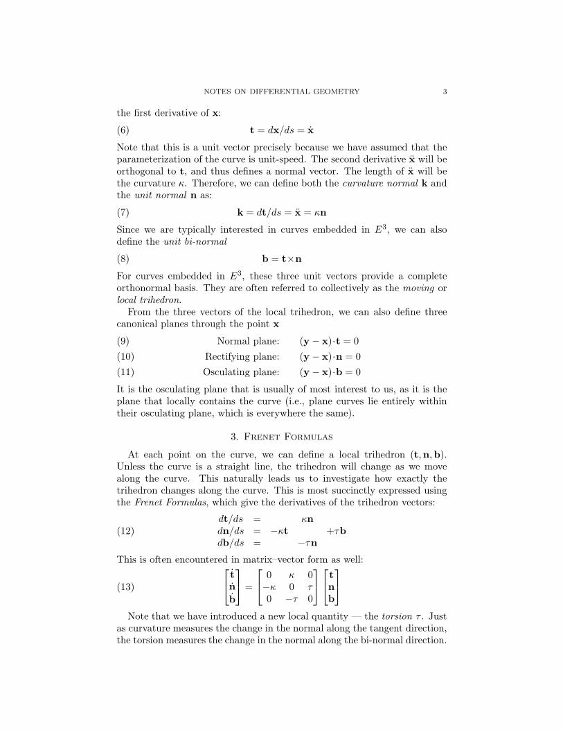
3. Frenet Formulas

At each point on the curve, we can define a local trihedron (t,n,b).Unless the curve is a straight line, the trihedron will change as we movealong the curve. This naturally leads us to investigate how exactly thetrihedron changes along the curve. This is most succinctly expressed usingthe Frenet Formulas, which give the derivatives of the trihedron vectors:

(12)dt/ds = κndn/ds = −κt +τbdb/ds = −τn

This is often encountered in matrix–vector form as well:

(13)

tnb

=

0 κ 0−κ 0 τ0 −τ 0

tnb

Note that we have introduced a new local quantity — the torsion τ . Just

as curvature measures the change in the normal along the tangent direction,the torsion measures the change in the normal along the bi-normal direction.

4 MICHAEL GARLAND

Intuitively, the torsion measures the differential “twisting” of the trihedronaround the curve.

Interpreted kinematically, the motion of the local trihedron can be seen asa differential translation (dx = t ds) combined with a differential rotation.The axis of this rotation, often referred to as the vector of Darboux, is simply

(14) r = τt + κb

This allows us to rewrite the Frenet equations in the following way

(15) t = r×t n = r×n b = r×b

Also note that r can be seen as an angular velocity vector, and thus ω = ‖r‖is the speed with which the trihedron is rotating.

We can perform a Taylor expansion of x around some point x(s0):

(16) x(s0 + h) = x(s0) + hx(s0) +h2

2x(s0) + · · ·

which leads to the following approximation of x in the neighborhood of apoint x(s0):

(17) x(s0 + h) ≈ x0 + ht0 + κ0h2

2n0 + κ0τ0

h3

6b0


Part 2. Geometry of Surfaces

Let us assume that we are given a closed differentiable manifold surfaceM which has been divided into a set of patches. A given surface patch isdefined by the mapping

(18) x = x(u, v) =

f1(u, v)f2(u, v)f3(u, v)

where (u, v) range over a region of the Cartesian 2-plane and the functions fi

are of class C2. We shall be concerned with the surface in the neighborhoodof a point p = x(u0, v0). By convention, all functions of x and its derivativesare implicitly evaluated at (u0, v0).

4. The Tangent Plane

The partial derivatives of the patch function x

(19) x1 = xu = ∂x/∂u and x2 = xv = ∂x/∂v

span the tangent plane of the surface at p, provided we make the standardassumption that x1×x2 6= 0.

Let t be a vector tangent to the surface x at the point p. We knowthat we can write it as a linear combination t = α1x1 + α2x2. Therefore,we can also conveniently represent this tangent vector as a direction vector

u =[α1

α2

].

We will generally be concerned with differential tangent vectors, that wewill write as:

(20) dx = dux1 + dv x2

Here we have a corresponding direction vector u =[dudv

].

Given that we have two vectors spanning the tangent plane, we can alsocompute the local unit surface normal n at the point p:

(21) n =x1×x2

‖x1×x2‖

5. First Fundamental Form

We would like to compute the (squared) length of a given differentialtangent vector dx. As with any other vector in E3, we compute the squaredlength of this vector via the inner product dx ·dx. Expanding this innerproduct, we arrive at:

(22) dx·dx = du2 x1 ·x1 + 2du dv x1 ·x2 + dv2 x2 ·x2

This quadratic form is called the first fundamental form. The classical no-tation for this quadratic form, dating back to Gauss, was the following:

(23) ds2 = E du2 + 2F du dv + G dv2

6 MICHAEL GARLAND

For our purposes, it is more convenient to write this quadratic form usingmatrix/vector notation. Assuming that we are given a direction vector u =[du dv]T, then we can write the first fundamental form as:

(24) dx·dx = uTGu where G =[g11 g12

g21 g22

]with gij = xi ·xj

The matrix G is usually referred to as the metric tensor. Since the dotproduct is commutative, it is clear that gij = gji and thus G is symmetric.We will also frequently have need to use the determinant of the metric tensor:

(25) g = detG = g11g22 − g212

Notice that our assumption that x1×x2 6= 0 implies that g 6= 0.We can also use the metric tensor to measure the angle between two

tangent vectors. Suppose we are given two direction vectors u and v. Theangle θ between them is characterized by:

(26) cos θ =uTGv

(uTGu)(vTGv)

In the special case of the angle θ between the two isoparametric lines thisreduces to:

(27) cos θ =g12√g11g22

sin θ =√

g

g11g22

5.1. The Jacobian. The Jacobian matrix of our surface patch x is thematrix of partial derivatives:

(28) J =

∂f1/∂u ∂f1/∂v∂f2/∂u ∂f2/∂v∂f3/∂u ∂f3/∂v

=

...

...x1 x2...

...

The metric tensor G can also be derived as the product of the Jacobian

with its transpose:

(29) G = JTJ =[x1

x2

][x1 x2] =

[x1 ·x1 x1 ·x2

x1 ·x2 x2 ·x2

]The Jacobian also provides a convenient notation for connecting the dif-

ferential tangent dx with its direction vector u. Specifically, dx = Ju.

5.2. Element of Area. Because it measures lengths and angles, the firstfundamental form is also the key to defining surface area. Suppose that weare given a region Ω on our surface patch x. Its area is given by the integral

(30)∫∫Ω

dA =∫∫

√g du dv

The differential dA =√

g du dv is referred to as the element of area of thesurface.


6. Second Fundamental Form

Suppose that we wish to measure the change of the normal vector n in agiven tangential direction: −dx ·dn. This is the second fundamental form.Like the first fundamental form, it also has a classical Gaussian notation:

(31) Ldu2 + 2M du dv + N dv2

We will generally work with the second fundamental form in its matrixversion:

(32) −dx·dn = uTBu where bij = n·xij = −ni ·xj .

As with the first fundamental form, we define the determinant of this tensor

(33) b = detB = b11b22 − b212

7. Surface Curvature

We have already seen in Section 2 how to define the curvature of a spacecurve. We can readily extend this definition to define the curvature of asurface as well.

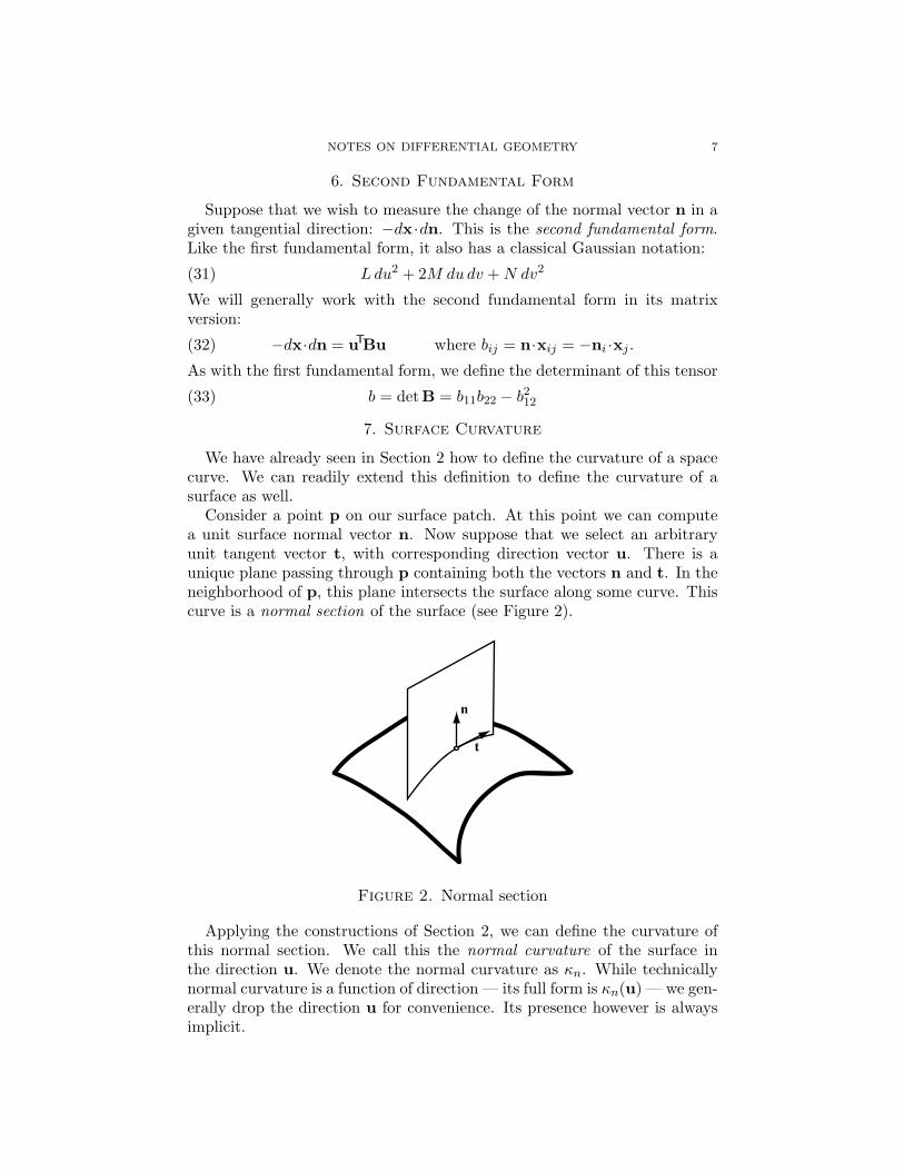
Consider a point p on our surface patch. At this point we can computea unit surface normal vector n. Now suppose that we select an arbitraryunit tangent vector t, with corresponding direction vector u. There is aunique plane passing through p containing both the vectors n and t. In theneighborhood of p, this plane intersects the surface along some curve. Thiscurve is a normal section of the surface (see Figure 2).

n

t

Figure 2. Normal section

Applying the constructions of Section 2, we can define the curvature ofthis normal section. We call this the normal curvature of the surface inthe direction u. We denote the normal curvature as κn. While technicallynormal curvature is a function of direction — its full form is κn(u) — we gen-erally drop the direction u for convenience. Its presence however is alwaysimplicit.

8 MICHAEL GARLAND

This definition of normal curvature is the most convenient intuitive defin-tion. We can also define it algebraically in terms of the fundamental forms.In particular, the normal curvature κn in the direction u is

(34) κn =uTBuuTGu

7.1. Principal Curvatures. Unless the curvature is equal in all directions,there must be a direction e1 in which the normal curvature reaches a max-imum and a direction e2 in which it reaches a minimum. These directionsare called principal directions and the corresponding curvatures κ1, κ2 arethe principal curvatures. It also turns out that the normal curvature κn inan arbitrary direction can be written in terms of the principal curvatures:

(35) κn = κ1 cos2 θ + κ2 sin2 θ

where θ is the angle between the direction in question and the first principaldirection.

In addition to the principal curvatures, we are also interested in twoimportant quantities. The first is the mean curvature

(36) H =12(κ1 + κ2)

The second is the Gaussian curvature

(37) K = κ1κ2

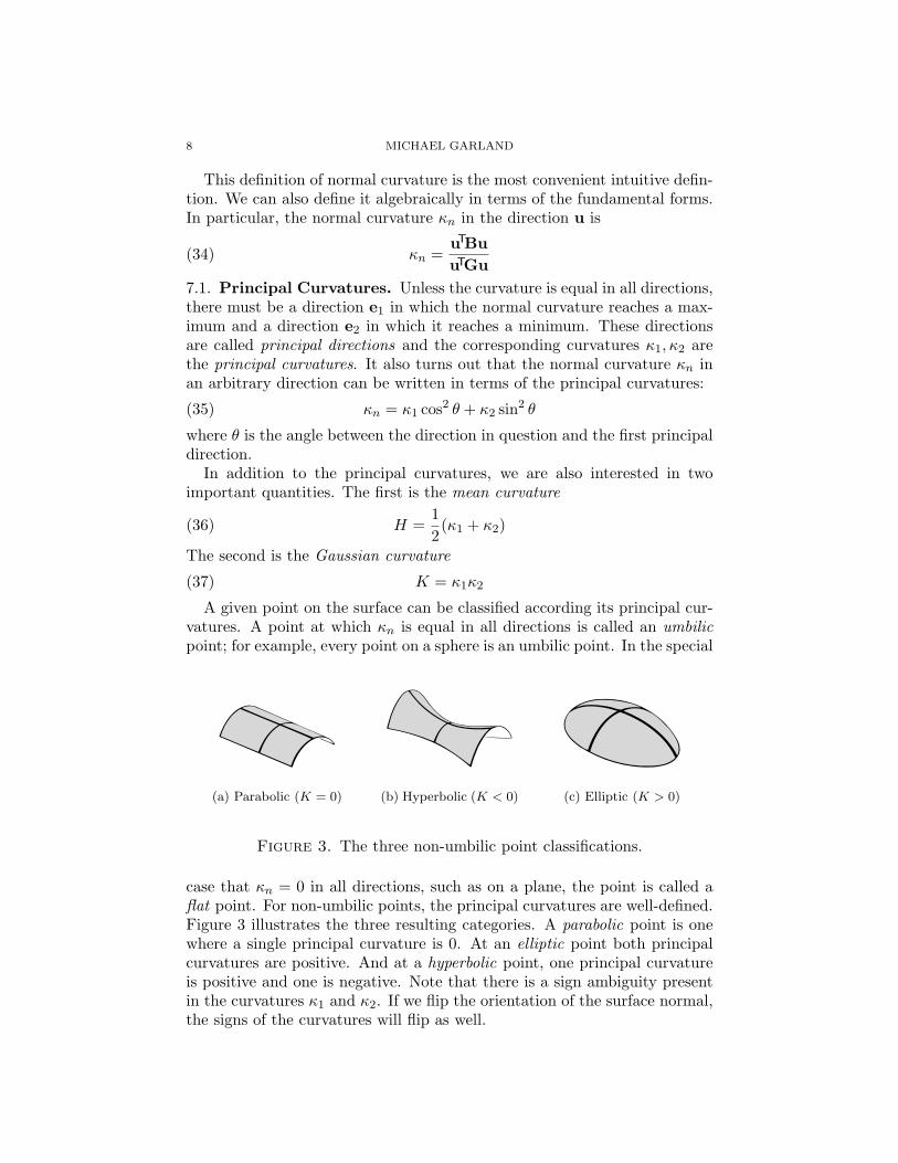
A given point on the surface can be classified according its principal cur-vatures. A point at which κn is equal in all directions is called an umbilicpoint; for example, every point on a sphere is an umbilic point. In the special

(a) Parabolic (K = 0) (b) Hyperbolic (K < 0) (c) Elliptic (K > 0)

Figure 3. The three non-umbilic point classifications.

case that κn = 0 in all directions, such as on a plane, the point is called aflat point. For non-umbilic points, the principal curvatures are well-defined.Figure 3 illustrates the three resulting categories. A parabolic point is onewhere a single principal curvature is 0. At an elliptic point both principalcurvatures are positive. And at a hyperbolic point, one principal curvatureis positive and one is negative. Note that there is a sign ambiguity presentin the curvatures κ1 and κ2. If we flip the orientation of the surface normal,the signs of the curvatures will flip as well.


All information about the local curvature of a surface can be encapsulatedin a single tensor

(38) S = G−1B

This tensor is variously called the curvature tensor, shape operator, and theWeingarten map. It has several important properties. Firstly, its eigenvaluesare the principal curvatures κ1, κ2. Its corresponding eigenvectors are theprincipal directions e1, e2. Because the principal curvatures of S, we alsoknow that the Gaussian curvature is

(39) K = detS =b

g

and the mean curvature is

(40) H =12

trS

8. Geodesics

Suppose that we’re given a unit-speed curve y that lies on the surfaceand passes through the point p. At this point, the curve has a unit tangentt = y and a unit normal m = y. The curvature vector κm of this curve canbe decomposed as

(41) κm = y = κnn + κgs

where n is the unit surface normal and s = n×t is tangent to the surface.The curvature κn is the normal curvature of the surface in the direction t.The curvature κg is called the geodesic curvature. Note that one consequenceof this equation is that

(42) κn = κ(m·n) = κ cos φ

where φ is the angle between the curve’s normal m and the surface normaln.

A geodesic curve is one whose geodesic curvature κg is everywhere 0. Fora point q in the vicinity of p, the curve passing through both p and q withshortest arc length between them will be a geodesic. Therefore, geodesicsare in an intuitive sense the “straight” lines intrinsic to a surface.

10 MICHAEL GARLAND

Part 3. Mappings

Given two surfaces M1 and M2, we are interested in exploring the proper-ties of functions f : M1 → M2 that provide a continuous mapping of pointson M1 into corresponding points on M2. We classify mappings based onthose geometric properties of the surface that they preserve. There are sev-eral classes of mappings that are commonly defined, but we are particularlyinterested in the following:

• Isometric mapping — preserves lengths.• Conformal mapping — preserves angles.• Equiareal mapping — preserves areas.• Geodesic mapping — the image of a geodesic is a geodesic.

In the following sections, we explore some of the specific properties ofthese mappings. Throughout this discussion, we assume that our attention isrestricted to a given patch of M1 parameterized by the function x : E2 → E3.This induces a parameterization y : E2 → E3 of the corresponding patch ofM2 where y = f x. We say that f is an allowable mapping if y meets ourbasic regularity requirement that y1×y2 6= 0. The parameterizations x,yof M1,M2 induce metrics G1,G2.

9. Isometric Mappings

Isometric mappings, or isometries, preserve lengths. This means that,for any curve C on M1, the lengths of C and f(C) are identical. Morespecifically, we can say that

(43)∫

Cds1 =

∫f(C)

ds2 for any curve C on M1

From this definition of isometry, it is fairly easy to prove that f is an iso-metric mapping if and only if G1 = G2.

Isometric mappings are a very restricted class of mappings. The require-ment that G1 = G2 implies that the two surface patches under consid-eration must have identical intrinsic geometries. One easy consequence ofthis is that isometric surfaces must have equal Guassian curvatures at everypair of corresponding points. Thus, the only surfaces that may be mappedisometrically into the plane are the developable surfaces.

10. Conformal Mappings

As stated above, conformal mappings are those that preserve angles. Con-sider two curves C,D on M1 meeting at a point p with angle θ. If f is aconformal mapping then their images, f(C) and f(D), will also meet withangle θ at f(p).

The class of conformal mappings is much broader than the class of isome-tries. Specifically, the mapping f is conformal if and only if G2 = cG1

for some smoothly varying local scale function c. If c is constant over the


entire surface, then f is in fact a similarity mapping and is for all practicalpurposes an isometry.

10.1. In the Plane. It is also fruitful to consider the simplest case of con-formal mappings in the plane. For a variety of reasons, it is convenient todiscuss such mappings in terms of complex-valued functions.

We define f : C → C in terms of a real part u and an imaginary part v:

(44) f(z) = u(z) + iv(z)

The function f is thus a mapping of the complex plane onto itself. Tosimplify our discussion somewhat, let us assume that u and v are real-valuedfunctions:

(45) f(x + iy) = u(x, y) + iv(x, y)

It turns out that f is a conformal map if and only if its derivative f ′ =df/dz exists. The requirement that f ′ exist is equivalent to the following:

(46)∂u

∂x=

∂v

∂yand

∂v

∂x= −∂u

∂y

These are the Cauchy-Riemann equations. They can also be restated in thefollowing form:

(47)(

∂u

∂x− ∂v

∂y

)+ i

(∂u

∂y+

∂v

∂x

)= 0

The Cauchy-Riemann equations provide the basic conditions for the ex-istance of the derivative f ′. Another important consequence is that if u, vsatisfy the Cauchy-Riemann equations, then they also satisfy Laplace’s equa-tion:

(48)∂2u

∂x2+

∂2u

∂y2= 0 and

∂2v

∂x2+

∂2v

∂y2= 0

The converse is, however, not true. Functions satisfying the Laplace equa-tion — which are called harmonic functions — do not necessarily satisfythe Cauchy-Riemann equations and are thus not necessarily conformal.

12 MICHAEL GARLAND

Part 4. Geometry of Discrete Manifolds

Up to this point, we have considered the geometry of differentiable man-ifolds. This is of course the setting in which differential geometry was de-veloped. However, discrete mesh representations of surfaces are at least ascommon as differentiable surfaces in the applications of interest to us. Inthis section, we briefly discuss the extension of many of the classical conceptsto the setting of discrete manifolds.

11. Notation and Conventions

We assume that we are dealing with a piecewise linear simplicial manifoldM = (V,E, F ) where V , E, and F are sets of vertices, edges, and faces. As-suming that each of the vertices in V is assigned an index, we represent bothedges and faces as tuples of vertex indices. Unless noted otherwise, thesesimplices are assumed to be oriented. This means that the pairs (i, j) and(j, i) both refer to the same edge connecting vertices i and j, but with oppo-site orientations. Similarly, the triangles (i, j, k) and (j, k, i) are equivalent,but (k, j, i) has opposite orientation.

As before, we will be concerned with the geometry of this surface whenembedded in the Euclidean space E3. We will denote the position of vertexi by xi. For a given oriented edge (i, j) — the edge from i to j — we definethe edge vector eij = xj − xi.

For a given triangle σ = (i, j, k), we can compute its surface normal nσ

from the cross product of its edge vectors:

(49) nσ =eij×eik

‖eij×eik‖

Mirroring the continuous case, we assume that ‖eij×eik‖ 6= 0. Furthermore,it is important to note that

(50) Area(σ) =12‖eij×eik‖

For a given vertex i, let Ni denote the set of vertices adjacent to the givenvertex.

(51) Ni = j | (i, j) ∈ E

Similarly, let Si denote the set of edges opposite the vertex i

(52) Si = (j, k) | (i, j, k) ∈ F

and let Ti be the set of faces incident on i.

(53) Ti = σ | i ∈ σ and σ ∈ F


12. Calculus on Simplicial Manifolds

It is important to remember that the development of a discrete differentialgeometry is an active area of research. There is as yet no one agreed uponframework for doing this. The development presented here is one possible —and reasonably consistent — avenue for discretizing classical notions. Butthere are others.

12.1. Functions and Vector Fields. We will generally be concerned withcontinuous piecewise linear functions defined over the mesh. In particular,we will regard a function f as a mapping

(54) f : V → R

and will denote by fi the value assigned by f to vertex i. This induces avalue f(x) for any point x on the surface, computed by linear interpolationwithin the triangle (i, j, k) containing x.

As we will see, many of the operations we wish to perform on functions ofthis sort are themselves linear. Therefore, it will at times be convenient toidentify the function f with a vector f ∈ Rn were n = |V |. In this case, thevalue of f at vertex i is simply the i-th component (i.e., fi) of an n-vector.

Defining tangent vector fields on discrete manifolds is somewhat moredifficult than in the continuous case. On a differentiable manifold, everypoint has a well defined tangent plane. For a triangulated manifold, this istrue only of points within a triangle. A vertex has no true tangent plane,although we frequently construct an approximate tangent plane by somelocal averaging procedure.

Because only triangles can truly be said to have a tangent plane, wewill generally restrict our discussion of tangent vectors to those which liein a specific triangle. We will therefore view a tangent vector field v as apiecewise constant vector-valued function

(55) v : F → R3

assigning a single tangent vector vσ to each triangle σ ∈ F . Although it isgenerally convenient to think of vσ as a 3-vector, it is a tangent vector, andthus always satisfies vσ ·nσ = 0. It is therefore always possible to representvσ as a 2-vector in some suitable orthonormal basis local to the triangle.

12.2. Gradients. Given a piecewise linear function f defined over our mesh,we naturally want to develop some suitable notion of the derivative of f .This is easily done by a suitable definition for the gradient of f . We definethe gradient ∇f to be a tangent vector field

(56) ∇f : F → R3

We will denote the gradient vector within a face σ by gσ. Note that thegradient vector has two important properties. First of all, it must lie in the

14 MICHAEL GARLAND

plane of the triangle; therefore it must be the case that gσ ·nσ = 0. It alsoallows as to express the restriction of f over σ as the linear function:

(57) fσ(x) = gσ ·x + bσ

This definition of gradient also allows us to easily define a notion of di-rectional derivative. Given any tangent vector v in the plane of the triangleσ, the directional derivative of f along v is:

(58) ∇vf = ∇f ·v = gσ ·v

Now, suppose that we select the edge vector e = xj − xi. The directionalderivative of f along the directed edge (i, j) is simply:

(59) ∇ef = fj − fi

This leads to a particularly straightforward way of computing the gradientof f . For the triangle σ = (i, j, k), the gradient vector gσ is the solution tothe linear system:

(60)

eij

ejk

nσ

gσ

=

fj − fi

fk − fj

0

12.3. Curl and Divergence. The definitions provided here are based onthose developed by Polthier and Preuß [14].

For a vector field in the plane, we are accustomed to analyzing its struc-ture in terms of quantities such as its curl and divergence. We can defineanalogous operators for tangent vector fields on discrete meshes. As before,we assume that the vector field v assigns a constant vector vσ to each tri-angle σ in the mesh. Furthermore, we will focus on defining the curl anddivergence of such a field at the vertices of the mesh.

At vertex i, we wish to compute curli v.

(61) curli v =12

∑σ=(j,k)∈Si

vσ ·ejk

Before providing the definition of divergence, we first define a tangentialrotation operator Rσ. We use this operator to indicate a counter-clockwiserotation by π/2 in the tangent plane of triangle σ. Obviously, Rσv = nσ×v.We can also write this transformation in matrix form as:

(62) R =

0 −n3 n2

n3 0 −n1

−n2 n1 0

where nσ = [n1 n2 n3 ]T.

We can now define the divergence of the vector field v at the vertex i as:

(63) divi v =∑

σ=(j,k)∈Si

vσ ·(Rejk) =∑

vσ ·(nσ×ejk)


Note that this is a sum over all the triangles adjacent to vertex i. It is alsoa fairly simple matter to show that this definition can be rewritten as a sumover all the vertices adjacent to i:

(64) divi v =12

∑j∈Ni

(cot αij + cot βij)(xj − xi)·v

where αij , βij are the angles opposite the edge (i, j), as illustrated in Fig-ure 4.

αθ

β

φ

vi

vj

Figure 4. Naming angles surrounding the edge (i, j).

12.4. Laplacian. Given a continuous function f : Rn → R, the Laplacianof f is defined to be:

(65) ∆f = ∇2f =n∑

i=1

∂2f

∂x2i

The discretization of this on a simplicial 2-manifold is a mapping

(66) ∆f : V → R

where

(67) ∆fi = −12

∑j∈Ni

(cot αij + cot βij)(fj − fi)

Note that this definition preserves the property that ∆f = div(∇f), as inthe continuous case.

For background on deriving this definition of the Laplacian, see Pinkalland Polthier [13], Duchamp et al. [5], and Desbrun et al. [2].

12.5. Discrete Differential Forms. A common formalism of modern cal-culus is the differential form. Indeed, some developments of the differentialgeometry of manifolds makes extensive use of differential forms1. In this sec-tion, we briefly outline an extension of differential forms to discrete surfaces(where, by rights, they probably ought to be called difference forms).

1In some older texts, you may encounter the use of the term Pfaffian. This is an olderterm, synonymous with differential form, that has fallen out of use.

16 MICHAEL GARLAND

A 0-form is simply a piecewise linear function f : V → R, assigning scalarvalues to vertices.

A 1-form ω assigns a scalar value to each oriented edge of M . It mustalso, by definition, satisfy the property that ωij = −ωji. It is thus anantisymmetric function ω : E → R.

A 2-form assigns scalar values to oriented triangles of M . As before, itmust also be antisymmetric, namely αijk = −αkji.

Given a piecewise linear function f defined at the vertices of M , thedifferential df : E → R is a 1-form given by

(68) dfij = fj − fi

Notice that this corresponds exactly with our definition of directional deriva-tives given in Section 12.2. Specifically, we can see that

(69) dfij = ∇ef where e = eij

which is, of course, exactly what we would expect.Given a 1-form ω, the differential dω is a 2-form. In a given triangle

(i, j, k) the value of this 2-form will be

(70) dωijk = ωij + ωjk + ωki

Note this obviously implies that d(df) = 0. It is equally apparent that∫C df = 0, for any closed cycle of edges C,

13. Discrete Curvature

As in the previous section, it is important to understand that the devel-opment of discrete notions of curvature is a research issue. Meyer et al. [11]provide a good discussion of the definitions that follow.

13.1. Gaussian Curvature. We can define the Gaussian curvature at ver-tex i by a direct discretization of the Gauss-Bonnet theorem:

(71) Ki = 2π −∑j∈Ti

θj

13.2. Mean Curvature. In the continuous case, it is well known that theLaplace-Beltrami operator provides a means of computing the mean curva-ture normal

(72) ∆x = xuu + xvv = 2κn

Given this equivalence, we can use our earlier discretization of the Laplacianover simplicial manifolds to produce an expression for the mean curvaturenormal at vertex i

(73) κini = ∆xi = −12

∑j∈Ni

(cot αij + cot βij)(xj − xi)


Part 5. Further Reading

A comprehensive introduction to differential geometry is clearly far be-yond the scope of these notes. Fortunately, there are a wide variety of booksavailable on the subject. The classic text of Hilbert and Cohn-Vossen [7]provides an excellent introduction to the intuitive side of the subject matterwith a minimum of formalism. Besl and Jain [1] give a nice overview of theessential material, and they discuss some computational techniques. For amore comprehensive and systematic treatment of the subject, I have foundKreyszig’s text [8] — an expanded version of an earlier book [9] — to befairly useful. Kreyszig’s book uses the more modern tensor notation. Will-more [16] provides a fairly easy to read introduction using the somewhatdated classical notation. O’Neill [12] is a widely used and well written intro-ductory book that uses the third major notation system, based on covariantdifferentiation, vector fields, and the shape operator.

Laugwitz [10] provides an admirably terse presentation of a truly im-pressive amount of material. Unfortunately, the notation can be a littleconfusing. Reading this book requires careful attention, but it’s a valuablereference. Struik [15] is a fair text that uses the classical notation. It’s bestfeature is the amount of historical background it provides. The book bydo Carmo [3] seems to fairly popular and he has more recently written acompanion book on Riemannian geometry [4]. You might also consider thebook by Gray [6] that provides fairly extensive examples that can be usedwith Wolfram’s Mathematica software.

References

[1] Paul J. Besl and Ramesh C. Jain. Invariant surface characteristics for 3D object recog-nition in range images. Computer Vision, Graphics, and Image Processing, 33:33–80,1986.

[2] Mathieu Desbrun, Mark Meyer, Peter Schroder, and Alan H. Barr. Implicit fairing ofirregular meshes using diffusion and curvature flow. In Proceedings of SIGGRAPH 99,Computer Graphics Proceedings, Annual Conference Series, pages 317–324, August1999.

[3] Manfredo do Carmo. Differential Geometry of Curves and Surfaces. Prentice Hall,1976.

[4] Manfredo do Carmo. Riemannian Geometry. Birkhauser Verlag, 1994.[5] T. Duchamp, A. Certain, A. DeRose, and W. Stuetzle. Hierarchical computation of

PL harmonic embeddings. preprint, July 1997.[6] Alfred Gray. Modern Differential Geometry of Curves and Surfaces with Mathematica.

CRC Press, Second edition, 1997.[7] D. Hilbert and S. Cohn-Vossen. Geometry and the Imagination. Chelsea, New York,

1952. Translated from the German Anschauliche Geometrie by P. Nemenyi.[8] Erwin Kreyszig. Introduction to Differential Geometry and Riemannian Geometry.

Number 16 in Mathematical Expositions. University of Toronto Press, Toronto, 1968.English translation — original German edition published in 1967 by AkademischeVerlagsgesellschaft.

[9] Erwin Kreyszig. Differential Geometry. Dover, New York, 1991. Reprint of 1959 edi-tion published by University of Toronto Press as Mathematical Expositions No. 11.

18 MICHAEL GARLAND

[10] Detlef Laugwitz. Differential and Riemannian Geometry. Academic Press, New York,1965. English translation by Fritz Steinhardt — original German edition, Differen-tialgeometrie, published in 1960 by B. G. Teubner.

[11] Mark Meyer, Mathieu Desbrun, Peter Schroder, and Alan H. Barr. Discretedifferential-geometry operators for triangulated 2-man ifolds. In Hans-Christian Hegeand Konrad Polthier, editors, Visualization and Mathematics III, pages 35–57.Springer-Verlag, Heidelberg, 2003.

[12] Barrett O’Neill. Elementary Differential Geometry. Academic Press, Boston, 1966.[13] Ulrich Pinkall and Konrad Polthier. Computing discrete minimal surfaces and their

conjugates. Experimental Mathematics, 2(1):15–36, 1993.[14] Konrad Polthier and Eike Preuss. Identifying vector field singularities using a discrete

Hodge decomposition. In Hans-Christian Hege and Konrad Polthier, editors, Visual-ization and Mathematics III, pages 113–134. Springer-Verlag, Heidelberg, 2003.

[15] Dirk J. Struik. Lectures on Classical Differential Geometry. Dover, New York, Secondedition, 1988. Reprint of 1961 edition published by Addison-Wesley.

[16] T. J. Willmore. An Introduction to Differential Geometry. Oxford University Press,London, 1959.

notes on differential geometry part 1. geometry of curves

Documents