notes on fluid dynamics - dicat.unige.it · notes on fluid dynamics rodolfo repetto department of...
TRANSCRIPT

Notes on Fluid Dynamics
Rodolfo Repetto
Department of Civil, Chemical and Environmental EngineeringUniversity of Genoa, [email protected]
phone number: +39 010 3532471http://www.dicca.unige.it/rrepetto/
skype contact: rodolfo-repetto
January 7, 2015
Rodolfo Repetto (University of Genoa) Fluid dynamics January 7, 2015 1 / 179
Table of contents I
1 Acknowledgements
2 Stress in fluidsThe continuum approachForces on a continuumThe stress tensorTension in a fluid at rest
3 Statics of fluidsThe equation of staticsImplications of the equation of staticsStatics of incompressible fluids in the gravitational fieldEquilibrium conditions at interfacesHydrostatic forces on flat surfacesHydrostatic forces of curved surfaces
4 Kinematics of fluidsSpatial and material coordinatesThe material derivativeDefinition of some kinematic quantitiesReynolds transport theoremPrinciple of conservation of massThe streamfunctionThe velocity gradient tensorPhysical interpretation of the rate of deformation tensor DPhysical interpretation of the rate of rotation tensor Ω
Rodolfo Repetto (University of Genoa) Fluid dynamics January 7, 2015 2 / 179

Table of contents II
5 Dynamics of fluidsMomentum equation in integral formMomentum equation in differential formPrinciple of conservation of the moment of momentumEquation for the mechanical energy
6 The equations of motion for Newtonian incompressible fluidsDefinition of pressure in a moving fluidConstitutive relationship for Newtonian fluidsThe Navier-Stokes equationsThe dynamic pressure
7 Initial and boundary conditionsInitial and boundary conditions for the Navier-Stokes equationsKinematic boundary conditionContinuity of the tangential component of the velocityDynamic boundary conditionsTwo relevant cases
8 Scaling and dimensional analysisUnits of measurement and systems of unitsDimension of a physical quantityQuantities with independent dimensionsBuckingham’s Π theoremDimensionless Navier-Stokes equations
Rodolfo Repetto (University of Genoa) Fluid dynamics January 7, 2015 3 / 179

Table of contents III
9 Unidirectional flowsIntroduction to unidirectional flowsSome examples of unidirectional flowsUnsteady unidirectional flowsAxisymmetric flow with circular streamlines
10 Low Reynolds number flowsIntroduction to low Reynolds number flowsSlow flow past a sphereLubrication Theory
11 High Reynolds number flowsThe Bernoulli theoremVorticity equation and vorticity productionIrrotational flowsBernoulli equation for irrotational flows
12 Introduction to numerical methodsWhat is computational fluid dynamicsA short introduction to numerical solutions of differential equationsA problem governed by an ODE: the Windkessel modelSimple integration schemes for ODEs
13 Appendix A: material derivative of the JacobianDeterminantsDerivative of the Jacobian
Rodolfo Repetto (University of Genoa) Fluid dynamics January 7, 2015 4 / 179
Table of contents IV
14 Appendix B: the equations of motion in different coordinates systemsCylindrical coordinatesSpherical polar coordinates
15 References
Rodolfo Repetto (University of Genoa) Fluid dynamics January 7, 2015 5 / 179
Acknowledgements
Acknowledgements
These lecture notes were originally written for the course in “Fluid Dynamics”, taught in L’Aquilawithin the MathMods, Erasmus Mundus MSc Course.A large body of the material presented here is based on notes written by Prof. Giovanni Seminarafrom the University of Genoa to whom I am deeply indebted. Further sources of material havebeen the following textbooks:
Acheson (1990),
Aris (1962),
Barenblatt (2003),
Batchelor (1967),
Ockendon and Ockendon (1995),
Pozrikidis (2010).
I wish to thank Julia Meskauskas (University of L’Aquila) and Andrea Bonfiglio (University ofGenoa) for carefully checking these notes.Very instructive films about fluid motion have been released by the National Committee for FluidMechanics and are available at the following link: http://web.mit.edu/hml/ncfmf.html
Rodolfo Repetto (University of Genoa) Fluid dynamics January 7, 2015 6 / 179

Stress in fluids
The state of stress in fluids
Rodolfo Repetto (University of Genoa) Fluid dynamics January 7, 2015 7 / 179

Stress in fluids The continuum approach
The continuum approach I
Definition of a simple fluidThe characteristic property of fluids (both liquids and gases) consists in the ease with which theycan be deformed.
A proper definition of a fluid is not easy to state as, in many circumstances, it is not obvious todistinguish a fluid from a solid.
In this course we will deal with “simple fluids”, which Batchelor (1967) defines as follows.
“A simple fluid is a material such that the relative positions of elements of the material change by
an amount which is not small when suitable chosen forces, however small in magnitude, are
applied to the material. . . . In particular a simple fluid cannot withstand any tendency by applied
forces to deform it in a way which leaves the volume unchanged.”
Note: the above definition does not imply that there will not be resistance to deformation.Rather, it implies that this resistance goes to zero as the rate of deformation vanishes.
Microscopic structure of fluids
The macroscopic properties of solids and fluids are relatedto their molecular nature and to the forces acting betweenmolecules. In the figure a qualitative diagram of the forcebetween two molecules as a function of their distance d isshown.d < d0 → repulsion; d > d0 → attraction, whered0 ≈ 10−10 m.
forc
e
distance d
repulsion
attraction
d0
Rodolfo Repetto (University of Genoa) Fluid dynamics January 7, 2015 8 / 179

Stress in fluids The continuum approach
The continuum approach II
Let d be the average distance between molecules. We have
gases → d >> d0;
solids and liquids → d ≈ d0.
In solids the relative position of particles is fixed, in fluids (liquids and gases) it can be freelyrearranged.
Continuum assumptionMolecules are separated by voids and the percentage of volume occupied by molecules is verysmall compared to the total volume.
In most applications of fluid mechanics the typical spatial scale L under consideration is muchlarger than the spacing between molecules d . We can then suppose that the behaviour of thefluid is the same as if the fluid was perfectly continuous in structure. This means that anyphysical property of the fluid, say f , can be regarded as a continuous function of space x (andpossibly time t)
f = f (x, t).
In order for the continuum approach to be valid it has to be possible to find a length scale L∗
which is much smaller than the smallest spatial scale at which macroscopic changes take placeand much larger than the microscopic (molecular) scale.
For instance in fluid mechanics normally a length scale L∗ = 10−5 m is much smaller than thescale of macroscopic changes but still we have L∗ ≫ d .
Rodolfo Repetto (University of Genoa) Fluid dynamics January 7, 2015 9 / 179
Stress in fluids Forces on a continuum
Forces on a continuum I
Two kind of forces can act on a continuum body:
long distance forces;
short distance forces.
Long distance forcesSuch forces are slowly varying in space. This means that if we consider a small volume δV theforce is approximately constant over it. Therefore, we may write
δF = fδV .
As long distance forces are proportional to the volume of fluid they act on, they are referred to asvolume or body forces. In most cases of interest for this course δF will be proportional to themass of the element
δF = ρfδV ,
where ρ denotes density, i.e. mass per unit volume. The dimensions of ρ are [ρ] = ML−3 (with M
mass and L length), and in the International System (SI) it is measured in kg m−3.The vector field f is denominated body force field. f has the dimension of an acceleration, orforce per unit mass [f] = LT−2 (with T time), and in the SI it is measured in m/s2.In general f depends on space and time: f = f(x, t). If we want to compute the force F on a finitevolume V we need to integrate f over V
F =
∫∫∫
V
ρfdV .
Rodolfo Repetto (University of Genoa) Fluid dynamics January 7, 2015 10 / 179

Stress in fluids Forces on a continuum
Forces on a continuum II
Short distance forces
Such forces are extremely rapidly variable in space and they act on very short distances. Thismeans that short distance forces are only felt on the surface of contact between adjacent portionsof fluid. Therefore, we may write
δΣ = tδS .
As short distance forces are proportional to the surface they act on, they are referred to assurface forces. The vector t is denominated tension. The tension t has the dimension of a forceper unit surface [t] = FL−2 = ML−1T−2, and in the SI it is measured in Pa=N m−2.
The vector t depends on space x, time t and on the unit vector n normal to the surface on whichthe stress acts: t = t(x, t, n).
Convention: we assume that t is the force per unit surface that the fluid on the side of thesurface towards which n points exerts on the fluid on the other side.
Important note: t(−n) = −t(n).
If we want to compute the force Σ on a finite surface S we need integrating t over S :
Σ =
∫∫
S
tdS .
Note that, if S is a closed surface, Σ represents the force that the fluid outside of S exerts on thefluid inside.
Rodolfo Repetto (University of Genoa) Fluid dynamics January 7, 2015 11 / 179
Stress in fluids The stress tensor
The stress tensor I
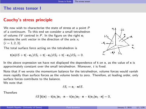
Cauchy’s stress principle
We now wish to characterise the state of stress at a point Pof a continuum. To this end we consider a small tetrahedronof volume δV centred in P. In the figure on the right eidenotes the unit vector in the direction of the axis xi(i = 1, 2, 3).
The total surface force acting on the tetrahedron is
t(n)δS + t(−e1)δS1 + t(−e2)δS2 + t(−e3)δS3 = 0.
In the above expression we have not displayed the dependence of t on x, as the value of x isapproximately constant over the small tetrahedron. Moreover, t is fixed.
Note that if we wrote the momentum balance for the tetrahedron, volume forces would vanishmore rapidly than surface forces as the volume tends to zero. Therefore, at leading order, onlysurface forces contribute to the balance.We note that
δSi = ei · nδS .Therefore
δS [t(n)− t(e1)e1 · n− t(e2)e2 · n− t(e3)e3 · n] = 0,
Rodolfo Repetto (University of Genoa) Fluid dynamics January 7, 2015 12 / 179

Stress in fluids The stress tensor
The stress tensor II
or, in index notation,
δS[ti (n)− ti (e1)e1jnj − ti (e2)e2jnj − ti (e3)e3jnj
]= 0.
Note that, throughout the course we will adopt Einstein notation or Einstein summationconvention. According to this convention, when an index variable appears twice in a single termof a mathematical expression, it implies that we are summing over all possible values of the index(typically 1, 2, 3). Thus, for instance
fjgj = f1g1 + f2g2 + f3g3 or fj∂fi
∂xj= f1
∂fi
∂x1+ f2
∂fi
∂x2+ f3
∂fi
∂x3.
We can now writeti (n) =
[ti (e1)e1j + ti (e2)e2j + ti (e3)e3j
]nj .
Since neither the vector t nor n depend on the coordinate system, the term in square brackets inthe above equation is also independent of it. Thus it represents a second order tensor, say σ (orin index notation σij ).We can thus write
ti (n) = σijnj , or, in vector notation, t(n) = σn. (1)
σij is named the Cauchy stress tensor, or simply stress tensor. σij represents the i component ofthe stress on the plane orthogonal to the unit vector ej .
Rodolfo Repetto (University of Genoa) Fluid dynamics January 7, 2015 13 / 179
Stress in fluids The stress tensor
The stress tensor III
Equation (1) implies that to characterise the stress in a point of a continuum we need a secondorder tensor, i.e. (given a coordinate system) 9 scalar quantities. We will show in the following(section 5) that σij is symmetric (σij = σji ), and therefore such scalar quantities reduce to 6.
The terms appearing in the principal diagonal of the matrix σij represent the so called normalstresses, those out of the principal diagonal are named tangential or shear stresses.
It is always possible to choose Cartesian coordinates such that σ takes a diagonal form
σI 0 00 σII 00 0 σIII
,
and σI , σII , σIII are named principal stresses and they are the eigenvalues of the matrixrepresenting σij . The corresponding directions are called principal directions.Obviously, the components of σij depend on the coordinate system but the stress tensor does notas it is a quantity with a precise physical meaning.
For any second order tensor it is possible to define 3 invariants, i.e. 3 quantities that do notdepend on the choice of the coordinate system. A commonly used set of invariants is given by
I1 = σI + σII + σIII = trσ = σjj , I2 = σIσII + σIIσIII + σIIIσI , I3 = σIσIIσIII = detσ.
Rodolfo Repetto (University of Genoa) Fluid dynamics January 7, 2015 14 / 179
Stress in fluids Tension in a fluid at rest
Tension in a fluid at rest I
The structure of σ in a fluid at rest is a consequence of the definition of simple fluid put forward.We consider a small spherical domain in a fluid at rest. Since the sphere is very small σ must beapproximately constant at all points within the sphere. We locally choose the principal axes sothat we can write σ as
σ =
σI 0 00 σII 00 0 σIII
.
We can now write σ = σ1 + σ2, where
σ1 =
1/3σjj 0 00 1/3σjj 00 0 1/3σjj
, σ2 =
σI − 1/3σjj 0 00 σII − 1/3σjj 00 0 σIII − 1/3σjj
.
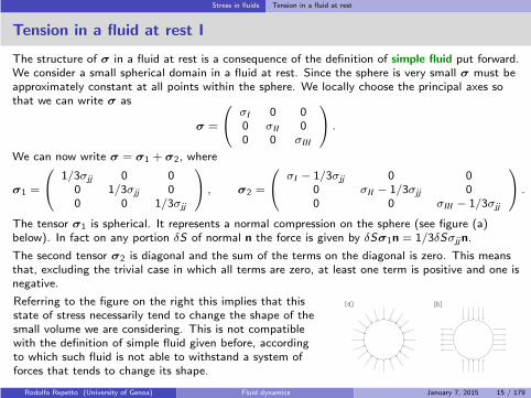
The tensor σ1 is spherical. It represents a normal compression on the sphere (see figure (a)below). In fact on any portion δS of normal n the force is given by δSσ1n = 1/3δSσjjn.
The second tensor σ2 is diagonal and the sum of the terms on the diagonal is zero. This meansthat, excluding the trivial case in which all terms are zero, at least one term is positive and one isnegative.
Referring to the figure on the right this implies that thisstate of stress necessarily tend to change the shape of thesmall volume we are considering. This is not compatiblewith the definition of simple fluid given before, accordingto which such fluid is not able to withstand a system offorces that tends to change its shape.
Rodolfo Repetto (University of Genoa) Fluid dynamics January 7, 2015 15 / 179

Stress in fluids Tension in a fluid at rest
Tension in a fluid at rest II
Therefore, σ2 must be equal to zero in a fluid at rest. Since fluids are normally in a state ofcompression we set
σij = −pδij , or, in vector form, σ = −pI, (2)
where the scalar quantity p is called pressure, and I is the identity matrix. Note that, due to theminus sign in the above equation, p > 0 implies compression. In general the pressure is a functionof space and time p(x, t). p has the dimension of a force per unit area([p] = FL−2 = ML−1T−2) and in the SI is measured in Pa.
Equation (2) implies that at a given point P of a fluid at rest the force acting on a small surfacepassing from P is equal to −pn, i.e. it is always normal to the surface and its magnitude does notdepend on the orientation of the surface.
Note: in some textbooks (2) is assumed as an indirect definition of a simple fluid (Eulerassumption).
Rodolfo Repetto (University of Genoa) Fluid dynamics January 7, 2015 16 / 179

Statics of fluids
Statics of fluids
Rodolfo Repetto (University of Genoa) Fluid dynamics January 7, 2015 17 / 179
Statics of fluids The equation of statics
The equation of statics I
Equation of statics in integral form
Let V be a volume of fluid within a body of fluid at rest and let S be its bounding surface. Wewish to write the equilibrium equation for this volume. From the equilibrium of forces we have
∫∫∫
V
ρfdV +
∫∫
S
tdS = 0. (3)
Equation (2) allows to rewrite the above expression as
∫∫∫
V
ρfdV +
∫∫
S
−pndS = 0, (4)
which represents the integral form of the equation of statics. The above equation is oftenconveniently written in compact form as
F+Σ = 0, (5)
with F resultant of all body forces acting on V and Σ resultant of surface forces acting on S .
Rodolfo Repetto (University of Genoa) Fluid dynamics January 7, 2015 18 / 179

Statics of fluids The equation of statics
The equation of statics II
Equation of statics in differential form
Using Gauss theorem equation (4) can be written as
∫∫∫
V
ρf −∇pdV = 0.
Since V is arbitrary the following differential equation must hold
ρf −∇p = 0, or, in index notation, ρfi −∂p
∂xi= 0, (6)
which is the equation of statics in differential form.
Equilibrium to rotation
In principle, the above equation alone is not sufficient to ensure equilibrium as we also have toimpose an equilibrium balance to rotation. This can be written as
∫∫∫
V
ρx× fdV +
∫∫
S
−px× ndS = 0, (7)
Rodolfo Repetto (University of Genoa) Fluid dynamics January 7, 2015 19 / 179

Statics of fluids The equation of statics
The equation of statics III
or, in index notation, ∫∫∫
V
ρǫijkxj fkdV +
∫∫
S
−pǫijkxjnkdS = 0. (8)
Note: ǫijk is the alternating tensor. Its terms are all equal to zero unless when i , j and k aredifferent from each other, in which case ǫijk takes the values 1 or -1 depending if i , j and k are ornot in cyclic order. Thus, we have
i j k ǫijk1 2 3 13 1 2 12 3 1 12 1 3 -11 3 2 -13 2 1 -1
Applying Gauss theorem to equation (8) we have:
∫∫∫
V
ǫijk
[
ρxj fk − ∂
∂xk(pxj )
]
dV = 0.
Rodolfo Repetto (University of Genoa) Fluid dynamics January 7, 2015 20 / 179
Statics of fluids The equation of statics
The equation of statics IV
Carrying on the calculations:
∫∫∫
V
ǫijk
(
ρxj fk − ∂
∂xk(pxj )
)
dV =
∫∫∫
V
ǫijk
(
ρxj fk − xj∂p
∂xk− p
∂xj
∂xk
)
dV =
∫∫∫
V
ǫijk
(
ρxj fk − xj∂p
∂xk− pδjk
)
dV =
∫∫∫
V
ǫijk
(
ρxj fk − xj∂p
∂xk
)
dV −∫∫∫
V
pǫijkδjkdV = 0,
(9)
where δij is the Kronecker delta (δij = 0 if i 6= j and δij = 1 if i = j). The above equation isautomatically satisfied as the first integral vanishes due to equation (6) and ǫijkδij = 0 bydefinition.
Rodolfo Repetto (University of Genoa) Fluid dynamics January 7, 2015 21 / 179

Statics of fluids Implications of the equation of statics
Implications of the equation of statics
Let us now consider the equation of statics (6). In order to integrate this equation we need anequation of state for the fluid, stating how the density ρ depends on the other physical propertiesof the fluid, and in particular p.
However, some general conclusions can be drawn by simple inspection of the equation.
As a first consideration we note that not all f(x) and p(x) allow for a fluid to be at rest. Inparticular the relationship ρf(x) = ∇p implies that ρf(x) admits a potential W , so that
ρf(x) = −∇W .
In the particular case in which ρ = const, f has to be conservative.
If f is conservative we have that f = −∇φ. In this case we have
−ρ∇φ = ∇p.
Applying the curl to the above expression we find
−∇× (ρ∇φ) = ∇×∇p ⇒ −∇ρ×∇φ−ρ∇×∇φ =∇×∇p.
The above relationship implies that level surfaces of ρ and φ must coincide.
Rodolfo Repetto (University of Genoa) Fluid dynamics January 7, 2015 22 / 179

Statics of fluids Statics of incompressible fluids in the gravitational field
Statics of incompressible fluids in the gravitational field
We assume
ρ = const. In this case we say that the fluid behaves as if it was incompressible.
f is the gravitational body force field.
We consider a system of Cartesian coordinates (x1, x2, x3), with x3 vertical upward directed axis.The gravitational field can therefore be written as f = (0, 0,−g).
With the above assumptions equation (6) can be easily solved to get
p = −ρgx3 + const,
and, after rearrangement, we obtain Stevin law
x3 +p
γ= const, (10)
where γ is the specific weight of the fluid ([γ] = FL−3, measured in N m−3 in the SI).The quantity h = x3 + p/γ is called piezometric or hydraulic head. Stevin law implies that, in anincompressible fluid at rest, h is constant.
Rodolfo Repetto (University of Genoa) Fluid dynamics January 7, 2015 23 / 179

Statics of fluids Equilibrium conditions at interfaces
Equilibrium conditions at interfaces I
Surface tension
The fact that small liquid drops form in air and gasbubbles form in liquids can be explained by assumingthat a surface tension acts at the interface between thetwo fluids.
If we draw a curve across the interface we assume thata force per unit length of magnitude κ exists, actingon the surface containing the interface and in thedirection orthogonal to the curve. The dimension of κis [κ] = FL−1 = MT−2 ans in the SI is measured in Nm−1.
Drop of water on a leaf.
The existence of such a force can be explained considering what happens at molecular level, closeto the interface: due to the existence of the interface, there is no balance of molecular forcesacting on particles very close to the interface.
κ can be positive (traction force on the surface) or negative (compression force on the surface),depending on the two fluids in contact. In particular we have:
κ > 0 immiscible fluids;
κ < 0 miscible fluids.
Rodolfo Repetto (University of Genoa) Fluid dynamics January 7, 2015 24 / 179

Statics of fluids Equilibrium conditions at interfaces
Equilibrium conditions at interfaces II
Pressure jump across a curved surface
We consider an equilibrium interface between two fluids. This implies that κ = const on thesurface.
We consider a curved surface. Let O be a point on the surface and let us adopt a system ofcoordinates centred in O and such that the (x − y) plane is tangent to the surface. The equationof the surface is
F (x , y , z) = z − ζ(x , y) = 0. (11)
Note that ζ and its first derivatives are zero at (x , y) = (0, 0). Close to O the approximateexpression of the normal vector n is
n =∇F
|∇F | ≈(
− ∂ζ
∂x,− ∂ζ
∂y, 1
)
,
correct to the first order in the small quantities ∂ζ/∂x , ∂ζ/∂y .
The resultant of the tensile force on a small portion of the surface S containing O is given by
−κ∮
C
n× dx,
with n normal to the surface and dx a line element of the closed curve C bounding the surface S .Recalling the equation of the surface (11) we can write dx = (dx , dy , ∂ζ
∂xdx + ∂ζ
∂ydy).
Rodolfo Repetto (University of Genoa) Fluid dynamics January 7, 2015 25 / 179

Statics of fluids Equilibrium conditions at interfaces
Equilibrium conditions at interfaces III
If the surface is flat, n is uniform and the above integral is zero. If the surface is curved theresultant is directed, at leading order, along z and has magnitude
−κ∮
C
− ∂ζ
∂xdy +
∂ζ
∂ydx .
Green’s theorem states that∫∫
S
(∂g
∂x− ∂f
∂y
)
dxdy =
∮
C
fdx + gdy .
In the present case the above equation can be specified so that
f = − ∂ζ
∂y, g =
∂ζ
∂x.
Therefore we get:
κ
∮
C
∂ζ
∂xdy − ∂ζ
∂ydx = κ
∫∫
S
(∂2ζ
∂x2+∂2ζ
∂y2
)
dS ≈ κ
(∂2ζ
∂x2+∂2ζ
∂y2
)
O
S .
We finally find
κ
(∂2ζ
∂x2+∂2ζ
∂y2
)
= κ
(1
R1+
1
R2
)
,
Rodolfo Repetto (University of Genoa) Fluid dynamics January 7, 2015 26 / 179
Statics of fluids Equilibrium conditions at interfaces
Equilibrium conditions at interfaces IV
where R1 and R2 are radii of curvature of the surface along two orthogonal directions. Note thatit can be shown that 1
R1+ 1
R2is independent on the orientation chosen.
The above equation implies that, in order for a curved interface between two fluids to be inequilibrium, a pressure jump ∆p must exist across the surface so that
∆p = κ
(1
R1+
1
R2
)
. (12)
Rodolfo Repetto (University of Genoa) Fluid dynamics January 7, 2015 27 / 179
Statics of fluids Hydrostatic forces on flat surfaces
Hydrostatic forces on flat surfaces I
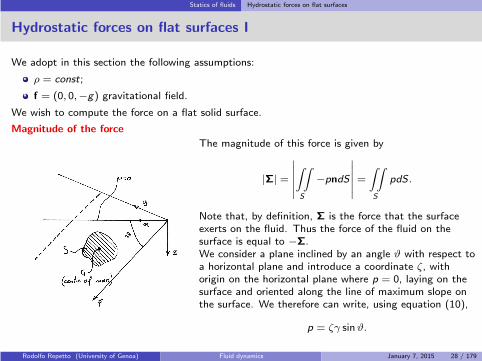
We adopt in this section the following assumptions:
ρ = const;
f = (0, 0,−g) gravitational field.
We wish to compute the force on a flat solid surface.
Magnitude of the force
The magnitude of this force is given by
|Σ| =
∣∣∣∣∣∣
∫∫
S
−pndS
∣∣∣∣∣∣
=
∫∫
S
pdS .
Note that, by definition, Σ is the force that the surfaceexerts on the fluid. Thus the force of the fluid on thesurface is equal to −Σ.We consider a plane inclined by an angle ϑ with respect toa horizontal plane and introduce a coordinate ζ, withorigin on the horizontal plane where p = 0, laying on thesurface and oriented along the line of maximum slope onthe surface. We therefore can write, using equation (10),
p = ζγ sinϑ.
Rodolfo Repetto (University of Genoa) Fluid dynamics January 7, 2015 28 / 179
Statics of fluids Hydrostatic forces on flat surfaces
Hydrostatic forces on flat surfaces II
Substituting in the definition of |Σ| we obtain
|Σ| =∫∫
S
ζγ sinϑdS = γ sinϑ
∫∫
S
ζdS = γ sinϑS, (13)
where S is the static moment of the surface S with respect to the axis y , defined as
S =
∫∫
S
ζdS . (14)
S can be written as S = ζGS , with ζG being the ζ coordinate of the centre of mass of S . Thuswe can write
|Σ| = γ sinϑζGS = γzGS = pGS , (15)
where z is a vertical coordinate directed downwards and with origin on the horizontal plane p = 0(see the figure of the previous page), and pG is the pressure in the centre of mass of S .
Equation (15) states that the magnitude of the force exerted by an incompressible fluid at restin the gravitational field on a flat surface is given by the product of the pressure pG at thecentre of mass of the surface and the area of the surface S .
Rodolfo Repetto (University of Genoa) Fluid dynamics January 7, 2015 29 / 179
Statics of fluids Hydrostatic forces on flat surfaces
Hydrostatic forces on flat surfaces III
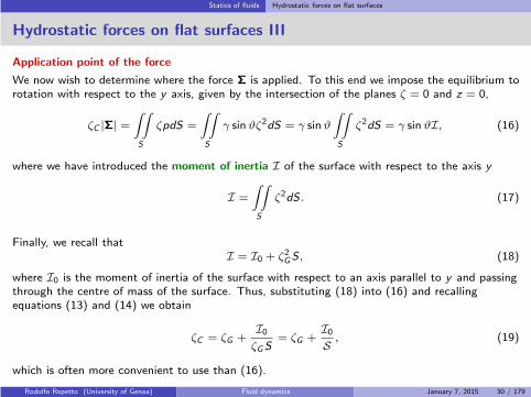
Application point of the force
We now wish to determine where the force Σ is applied. To this end we impose the equilibrium torotation with respect to the y axis, given by the intersection of the planes ζ = 0 and z = 0,
ζC |Σ| =∫∫
S
ζpdS =
∫∫
S
γ sinϑζ2dS = γ sinϑ
∫∫
S
ζ2dS = γ sinϑI, (16)
where we have introduced the moment of inertia I of the surface with respect to the axis y
I =
∫∫
S
ζ2dS . (17)
Finally, we recall thatI = I0 + ζ2GS , (18)
where I0 is the moment of inertia of the surface with respect to an axis parallel to y and passingthrough the centre of mass of the surface. Thus, substituting (18) into (16) and recallingequations (13) and (14) we obtain
ζC = ζG +I0ζGS
= ζG +I0S , (19)
which is often more convenient to use than (16).
Rodolfo Repetto (University of Genoa) Fluid dynamics January 7, 2015 30 / 179
Statics of fluids Hydrostatic forces of curved surfaces
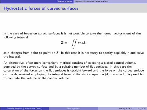
Hydrostatic forces of curved surfaces
In the case of forces on curved surfaces it is not possible to take the normal vector n out of thefollowing integral
Σ = −∫∫
S
pndS ,
as n changes from point to point on S . In this case it is necessary to specify explicitly n and solvethe integral.
An alternative, often more convenient, method consists of selecting a closed control volume,bounded by the curved surface and by a suitable number of flat surfaces. In this case thecalculation of the forces on the flat surfaces is straightforward and the force on the curved surfacecan be determined employing the integral form of the statics equation (4), provided it is possibleto compute the volume of the control volume.
Rodolfo Repetto (University of Genoa) Fluid dynamics January 7, 2015 31 / 179
Kinematics of fluids
Kinematics of fluids
Rodolfo Repetto (University of Genoa) Fluid dynamics January 7, 2015 32 / 179

Kinematics of fluids Spatial and material coordinates
Spatial and material coordinates I
The kinematics of fluids studies fluid motion per se, with no concern to the forces which generatethe motion. All kinematic notions that will be introduced in the present chapter are valid for anyfluid described as a continuum. A very good reference for kinematics of fluid is Aris (1962); thepresent section is largely based on this textbook.
Understanding how to study fluid motion from the kinematic point of view is a prerequisite tostudy the dynamics of fluids, which will be considered in the following chapter.
The basic mathematical idea is that, within the continuum approach, fluid motion can bedescribed by a point transformation.
Let us consider a fluid particle which at time t0 is located in the position ξ = (ξ1, ξ2, ξ3). Thesame particle at time t is at position x = (x1, x2, x3). Without loss of generality we can sett0 = 0. The motion of the particle in the time interval [0, t] is described by the function
x = x(ξ, t), or, in index notation, xi = xi (ξ1, ξ2, ξ3, t), (20)
which, at any time t, tells us the position in space of the particle that was in ξ at t = 0.
ξ are named material or Lagrangian coordinates as a particular value of ξ identifies thematerial particle that at t = 0 was in ξ.
x are named spatial or Eulerian coordinates as a particular value of x identifies a givenposition in space which might be occupied, at different times, by different fluid particles.
Rodolfo Repetto (University of Genoa) Fluid dynamics January 7, 2015 33 / 179

Kinematics of fluids Spatial and material coordinates
Spatial and material coordinates II
We assume that the motion is continuous, that at a given time a single particle cannot occupytwo different positions and, conversely, that a single point in space cannot be occupiedsimultaneously by two particles. This implies that equation (20) can be inverted to obtain
ξ = ξ(x, t), or, in index notation, ξi = ξi (x1, x2, x3, t). (21)
Equation (21) gives the initial position (at t = 0) of a material particle that at time t is in x.Mathematically, the condition of invertibility of (20) can be expressed as J > 0 (see Aris, 1962),where the Jacobian J is defined as
J = det
[∂(x1, x2, x3)
∂(ξ1, ξ2, ξ3)
]
. (22)
Knowledge of equation (20) or (21) is enough to completely describe the flow. The flow,however, can also be studied by describing how any fluid property, say F (e.g. density, pressure,velocity, . . . ) changes in time at any position in space.
F = F(x, t).
This approach is referred to as spatial approach or Eulerian approach.
Alternatively, we can describe the evolution of a fluid property F associated with a given fluidparticle. In this case we write
F = F(ξ, t).
Rodolfo Repetto (University of Genoa) Fluid dynamics January 7, 2015 34 / 179
Kinematics of fluids Spatial and material coordinates
Spatial and material coordinates III
Note that a given value of ξ identifies the particle that in t = 0 was in ξ. This approach isreferred to as material approach or Lagrangian approach.
Any physical property of the fluid can be expressed either in Eulerian or Lagrangian coordinates,and employing equations (20) and (21) we can change the description adopted
F(x, t) = F [ξ(x, t), t], (23)
F(ξ, t) = F [x(ξ, t), t]. (24)
Rodolfo Repetto (University of Genoa) Fluid dynamics January 7, 2015 35 / 179

Kinematics of fluids The material derivative
The material derivative I
The time derivative of a generic physical property of the fluid F has a different meaning inEulerian and Lagrangian coordinates.
Eulerian coordinates:∂F(x, t)
∂tlocal derivative.
This represents the variation in time of F at a given point in space. Such a point can, ingeneral, be occupied by different particles at different times.
Lagrangian coordinates:∂F(ξ, t)
∂tmaterial derivative.
This represents the time evolution of F associated with a given material particle.
Since the physical meaning of the two derivatives is different it is customary in fluid mechanics todenote them with different symbols.
∂
∂t≡(∂
∂t
)
x
≡ time derivative at constant x,
D
Dt≡(∂
∂t
)
ξ
≡ time derivative at constant ξ.
Rodolfo Repetto (University of Genoa) Fluid dynamics January 7, 2015 36 / 179

Kinematics of fluids The material derivative
The material derivative II
Note: If the fluid property F is the position of a material particle (F = xi ) we have
ui =Dxi
Dt, or in vector notation u =
Dx
Dt, (25)
which is the velocity of the fluid particle.
In general it is more convenient in fluid mechanics to adopt a spatial (Eulerian) description of theflow. However, for the definition of some physical quantities the material derivative is required.For instance the acceleration a is defined as
a =Du
Dt,
while ∂u/∂t 6= a, as it represents the rate of change of velocity at a fixed point in space, i.e. it isnot referred to a material particle.
It is then often necessary to define the material derivative in terms of spatial coordinates. Usingequations (24) and (25) we can write
DFDt
=∂F(ξ, t)
∂t=∂F [x(ξ, t), t]
∂t=
=
(∂F∂t
)
x
+∂F∂xi
(∂xi
∂t
)
ξ
=
=∂F∂t
+ ui∂F∂xi
.
Rodolfo Repetto (University of Genoa) Fluid dynamics January 7, 2015 37 / 179

Kinematics of fluids The material derivative
The material derivative III
Thus we find
DFDt
=∂F∂t
+ ui∂F∂xi
, or, in vector form,DFDt
=∂F∂t
+ u · ∇F . (26)
If F is a vector quantity we obtain
DFi
Dt=∂Fi
∂t+ uj
∂Fi
∂xj, or in vector form,
DF
Dt=∂F
∂t+ (u · ∇)F . (27)
Rodolfo Repetto (University of Genoa) Fluid dynamics January 7, 2015 38 / 179

Kinematics of fluids Definition of some kinematic quantities
Definition of some kinematic quantities I
Trajectories or particle pathsEquation (20) can be seen as a parametric equation of a curve in space, with t as parameter. Thecurve goes through the point ξ when t = 0. It represents the particle path or pathline or particletrajectory.
Particle trajectories can be obtained from a spatial description of the flow by integration of thespatial velocity field
dx
dt= u(x, t), x(0) = ξ. (28)
Steady flowThe velocity field in spatial coordinates is described by the vector field u(x, t). If u does notdepend on time the flow is said to be steady. Note that steadiness of flow does not imply thateach material particle has a constant velocity in time as u(ξ, t) might still depend on time.
StreamlinesGiven a spatial description of a velocity field u(x, t), streamlines are curves which are at all pointsin space parallel to the velocity vector. Mathematically, they are therefore defined as
dx× u = 0, (29)
Rodolfo Repetto (University of Genoa) Fluid dynamics January 7, 2015 39 / 179
Kinematics of fluids Definition of some kinematic quantities
Definition of some kinematic quantities II
with dx an infinitesimal segment along the streamline. The above expression can also be writtenas
dx1
u1=
dx2
u2=
dx3
u3. (30)
The unit vector dx/|dx| can be written as dx/ds, where the curve parameter s is the arc lengthmeasured from an initial point x0 = x(s = 0). Equation (29) then implies that
dx
ds=
u
|u| . (31)
Particle paths and streamlines are not in general coincident. However they are in the followingcases.
Steady flow. In this case the equation for a pathline is dxdt
= u(x). The element of the arclength along the pathline is ds = |u|dt, which, substituted in the above expression, yields
dx
ds=
u
|u| ,
which shows that, for a steady flow, the differential equation for pathlines and streamlinesare the same.
Rodolfo Repetto (University of Genoa) Fluid dynamics January 7, 2015 40 / 179

Kinematics of fluids Definition of some kinematic quantities
Definition of some kinematic quantities III
Unsteady flow the direction of which does not change with time. In this case we can writeu(x, t) = f (x, t)u0(x) with u0 the velocity field at the initial time. In this case the argumentused for steady flows still holds.
StreaklinesAt a given time t a streakline joins all material points which have passed through (or will passthrough) a given place x at any time.
Filaments of colour are often used to make flow visible. Coloured fluid introduced into the streamat place x0 forms a filament and a snapshot of this filament is a streakline.
Setting x = x′ and t = t′ in (21) identifies the material point which was at place x′ at time t′.The path coordinates of this particle are given by
x = x[ξ(x′, t′), t].
At a given time t, t′ is the curve parameter of a curve in space which goes through the givenpoint x′. This curve in space is a streakline.
In steady flows, streaklines, streamlines and pathlines are all coincident.
Uniform flowA flow is said to be uniform if u does not depend on x.
u = u(t).
Rodolfo Repetto (University of Genoa) Fluid dynamics January 7, 2015 41 / 179

Kinematics of fluids Definition of some kinematic quantities
Definition of some kinematic quantities IV
This is a very strong requirement. Sometimes the flow is called uniform if u does not changealong the streamlines.
Plane flowA flow is said to be plane or two-dimensional if it is everywhere orthogonal to one direction andindependent of translations along such direction.
In a plane flow it is therefore possible to choose a system of Cartesian coordinates (x1, x2, x3) sothat u has the form
u = (u1, u2, 0),
and u1 and u2 do not depend on x3.
Axisymmetric flowA flow is said to be axisymmetric if, chosen a proper system of cylindrical coordinates (z, r , ϕ)the velocity u = (uz , ur , uϕ) is independent of the azimuthal coordinate ϕ, and uϕ = 0.
Rodolfo Repetto (University of Genoa) Fluid dynamics January 7, 2015 42 / 179

Kinematics of fluids Reynolds transport theorem
Reynolds transport theorem I
Let F(x, t) be a property, either a scalar or a vector, of the fluid and V (t) a material volumeentirely occupied by the fluid. A material volume is a volume which is always constituted by thesame particles. We can define the integral
F (t) =
∫∫∫
V (t)
F(x, t)dV . (32)
We wish to evaluate the material derivative of F . Since V (t) depends on time the derivativeD/Dt can not be taken into the integral. However, if we work with material coordinates ξ, thevolume remains unchanged in time and equal to the value V0 it had at the initial time. We canthus write
D
Dt
∫∫∫
V (t)
F(x, t)dV =D
Dt
∫∫∫
V0
F(ξ, t)JdV0,
where dV = JdV0, with J Jacobian of the transformation, defined by (22). We can now write
∫∫∫
V0
JDFDt
+ F DJ
DtdV0.
It can be shown (see section 13) that
DJ
Dt= (∇ · u)J. (33)
Rodolfo Repetto (University of Genoa) Fluid dynamics January 7, 2015 43 / 179

Kinematics of fluids Reynolds transport theorem
Reynolds transport theorem II
The above integral can then be written as
∫∫∫
V0
[DFDt
+ F(∇ · u)]
JdV0,
and going back to the spatial coordinates x, we find
∫∫∫
V (t)
[DFDt
+ F(∇ · u)]
dV .
Finally, recalling (26), we have
D
Dt
∫∫∫
V (t)
F(x, t)dV =
∫∫∫
V (t)
[∂F∂t
+∇ · (Fu)
]
dV . (34)
This result is known as Reynolds transport theorem. The above expression can be also bewritten as
D
Dt
∫∫∫
V (t)
F(x, t)dV =
∫∫∫
V (t)
∂F∂t
dV +
∫∫
S(t)
Fu · ndA, (35)
Rodolfo Repetto (University of Genoa) Fluid dynamics January 7, 2015 44 / 179

Kinematics of fluids Reynolds transport theorem
Reynolds transport theorem III
with S(t) being the bounding surface of the volume V (t) and n the outer normal to this surface.Equation (35) shows that the material derivative of a variable F integrated over a materialvolume V (t) can be written as the integral of ∂F/∂t over the volume V (t) plus the flux of Fthrough the surface S(t) of this volume.
Rodolfo Repetto (University of Genoa) Fluid dynamics January 7, 2015 45 / 179
Kinematics of fluids Principle of conservation of mass
Principle of conservation of mass
Let us consider a material volume V with bounding surface S . The principle of conservation ofmass imposes that: the material derivative of the mass of fluid in V is equal to zero.
The mass of the fluid in V is given by ∫∫∫
V
ρdV .
Therefore we haveD
Dt
∫∫∫
V
ρdV = 0.
Recalling (34) we have:∫∫∫
V
∂ρ
∂t+∇ · (ρu)dV = 0. (36)
since the volume V is arbitrary the following differential equation holds
∂ρ
∂t+∇ · (ρu) = 0, or, in index notation,
∂ρ
∂t+
∂
∂xj(ρuj ) = 0. (37)
This equation is known in fluid mechanics as continuity equation.In the particular case in which the fluid is incompressible, i.e. the density ρ is constant, the aboveequation reduces to
∇ · u = 0, or, in index notation,∂uj
∂xj= 0. (38)
This implies that the velocity field of an incompressible fluid is divergence free.Rodolfo Repetto (University of Genoa) Fluid dynamics January 7, 2015 46 / 179
Kinematics of fluids The streamfunction
The streamfunction I
A differential formdf = p(x , y)dx + q(x , y)dy ,
is said to be an exact differential if∫df is path independent. This happens when
df =∂f
∂xdx +
∂f
∂ydy .
Therefore, in this case
p =∂f
∂x, q =
∂f
∂y,
and this implies∂p
∂y=∂q
∂x. (39)
Plane flow of an incompressible fluidLet us consider a plane flow on the (x1, x2) plane so that the velocity has only two components u1and u2. Let us also assume that the fluid is incompressible. The continuity equation (38) reducesto
∂u1
∂x1+∂u2
∂x2= 0.
Rodolfo Repetto (University of Genoa) Fluid dynamics January 7, 2015 47 / 179

Kinematics of fluids The streamfunction
The streamfunction II
The above expression implies that the following differential
dψ = −u2dx1 + u1dx2,
is exact, as the condition (39) is satisfied. Then we have
u1 =∂ψ
∂x2, u2 = − ∂ψ
∂x1, (40)
and the scalar function ψ(x1, x2, t) is defined as
ψ − ψ0 =
∫
(−u2dx1 + u1dx2). (41)
In the above expression ψ0 is a constant and the line integral is taken on an arbitrary path joiningthe reference point O to a point P with coordinates (x1, x2). We know that, as dψ is an exactdifferential, the value of ψ− ψ0 does not depend on the path of integration but only on the initialand finals points.
The function ψ has a very important physical meaning. The fluxof fluid volume across the line joining the points O and P (takenpositive if the flux is in the anti-clockwise direction about P) isgiven by the integral
∫
(−u2dx1 + u1dx2).
This means that the flux through any curve joining two points isequal to the difference of the value of ψ at these points.
Rodolfo Repetto (University of Genoa) Fluid dynamics January 7, 2015 48 / 179

Kinematics of fluids The streamfunction
The streamfunction III
Therefore the value of ψ is constant along streamlines as, by definition, the flux across anystreamline is zero. For this reason the function ψ is named streamfunction.The advantage of having introduced the streamfunction is that we can describe the flow using ascalar function rather than the vector function u.
Axisymmetric flow of an incompressible fluidLet us now consider an axisymmetric flow of an incompressible fluid.Let us assume a system of cylindrical coordinates (z, r , ϕ). The corresponding velocitycomponents are (uz , ur , uϕ). Due to the axisymmetry of the flow we know that uϕ = 0 and thatur and uz do not depend on ϕ. In this case the continuity equation (38) reads
∇ · u =∂uz
∂z+
1
r
∂rur
∂r= 0.
We can again define a streamfunction as
ur = −1
r
∂ψ
∂z, uz =
1
r
∂ψ
∂r, ψ − ψ0 =
∫
r(uzdr − urdz). (42)
The streamfunction for an incompressible axisymmetric flow can also be expressed in terms ofother orthogonal systems of coordinates, e.g. spherical polar coordinates, see equation (123).
Rodolfo Repetto (University of Genoa) Fluid dynamics January 7, 2015 49 / 179
Kinematics of fluids The velocity gradient tensor
The velocity gradient tensor I
Let us consider two nearby points P and Q with material coordinates ξ and ξ + dξ. At time t
their position is x(ξ, t) and x(ξ + dξ, t). We can relate the position of the two particles with thefollowing relationship
xi (ξ + dξ, t) = xi (ξ, t) +∂xi
∂ξjdξj + O(d2),
where O(d2) represents terms of order dξ2 or smaller that will be neglected. The smalldisplacement vector dξ at the time t has become dx = x(ξ + dξ, t)− x(ξ, t) and it takes theexpression
dxi =∂xi
∂ξjdξj . (43)
Definition: the quantity ∂xi∂ξj
is a tensor which is named displacement gradient tensor. This
tensor is fundamental in the theory of elasticity.
In fluid mechanics it is more significant to reason in terms of velocities (u = Dx/Dt). Therelative velocity of two particles with material coordinates ξ and ξ + dξ can be written as
dui =∂ui
∂ξjdξj =
D
Dt
(∂xi
∂ξj
)
dξj . (44)
Rodolfo Repetto (University of Genoa) Fluid dynamics January 7, 2015 50 / 179

Kinematics of fluids The velocity gradient tensor
The velocity gradient tensor II
Inverting (43) we can rewrite the above expression as
dui =∂ui
∂ξk
∂ξk
∂xjdxj =
∂ui
∂xjdxj . (45)
The above equation expresses the relative velocity in terms of the current relative position.
Definition: the quantity ∂ui∂xj
(or ∇u in vector form) is a tensor that is named velocity gradient
tensor.
In general ∇u is non symmetric. Any tensor can be decomposed into a symmetric and anantisymmetric part. In particular we can write
∂ui
∂xj=
1
2
(∂ui
∂xj+∂uj
∂xi
)
+1
2
(∂ui
∂xj− ∂uj
∂xi
)
, or in vector form ∇u = D+Ω. (46)
Above we have defined
Dij =1
2
(∂ui
∂xj+∂uj
∂xi
)
, rate of deformation tensor, (47)
Ωij =1
2
(∂ui
∂xj− ∂uj
∂xi
)
, rate of rotation tensor. (48)
Both the above tensors play a vey important role in fluid mechanics. Their physical meaning isexplained in the two following sections.
Rodolfo Repetto (University of Genoa) Fluid dynamics January 7, 2015 51 / 179
Kinematics of fluids Physical interpretation of the rate of deformation tensor D
Physical interpretation of the rate of deformation tensor I
We now wish to interpret the physical meaning of the rate of deformation tensor D. Let usconsider how a small material element of fluid deforms during motion. Let P and Q be two closematerial particles with coordinates ξ and ξ + dξ, whose positions at time t are x(ξ, t) andx(ξ + dξ, t). Let the length of the small segment connecting P and Q at time t be ds. Recalling(43) we can write
ds2 = dxidxi =∂xi
∂ξj
∂xi
∂ξkdξjdξk .
Let us now take the material derivative of ds2.
D
Dtds2 =
(∂ui
∂ξj
∂xi
∂ξk+∂xi
∂ξj
∂ui
∂ξk
)
dξjdξk = 2∂ui
∂ξj
∂xi
∂ξkdξjdξk .
Note that we have used the fact that dξj and dξk do not change in time as they are materialsegments. Moreover, we could swap j and k as they both are dummy indexes.Recalling (43), (44) and (45) we know that
∂ui
∂ξjdξj =
∂ui
∂xjdxj ,
∂xi
∂ξkdξk = dxi .
Therefore, we can write
1
2
D
Dtds2 = ds
D
Dtds =
∂ui
∂xjdxidxj = Dijdxidxj .
Rodolfo Repetto (University of Genoa) Fluid dynamics January 7, 2015 52 / 179

Kinematics of fluids Physical interpretation of the rate of deformation tensor D
Physical interpretation of the rate of deformation tensor II
In the above expression we have used the fact the antisymmetric terms in ∂ui/∂xj vanish uponsummation and, therefore, only the symmetric part of the velocity gradient tensor (i.e. Dij )survives.The above expression can also be rewritten as
1
ds
D
Dtds = Dij
dxi
ds
dxj
ds. (49)
The term dxi/ds is the i th component of a unit vector in the direction of the segment PQ.Therefore equation (49) states that the rate of change of the length of the segment (as a fractionof its length) is related to its direction through the deformation tensor D.We can also observe that if D = 0 the segment PQ remains of constant length. Therefore we canstate that if D = 0 the motion is locally and instantaneously rigid. The tensor D is thereforerelated to deformation of material elements.
Meaning of the terms on the main diagonal of D
Let PQ be parallel to the coordinate axis x1. In this casedx
ds= e1, with e1 unit vector in the
direction of x1. Then equation (49) simplifies to
1
dx1
D
Dtdx1 = D11.
Rodolfo Repetto (University of Genoa) Fluid dynamics January 7, 2015 53 / 179

Kinematics of fluids Physical interpretation of the rate of deformation tensor D
Physical interpretation of the rate of deformation tensor III
Thus the element D11 represents the rate of longitudinal strain of an element parallel to x1.Obviously, the same interpretation applies to the other two terms on the main diagonal of D, i.e.D22 and D33.
Meaning of the terms out of the main diagonal of D
We now consider two segments PQ and PR, where R is amaterial particle with material coordinates ξ + dξ′. Let ds′ bethe length of the segment PR and θ the angle between thesegments PQ and PR. We then have
ds ds′ cos θ = dxidx′i .
Taking the material derivative of the above expression, using again (45), we have
D
Dt(ds ds′ cos θ) = duidx
′i + dxidu
′i =
∂ui
∂xjdxjdx
′i + dxi
∂ui
∂xjdx ′j .
As i and j are dummy indexes they can be interchanged, and we can then write
cos θ
(1
ds
D
Dtds +
1
ds′
D
Dtds′)
− sin θDθ
Dt=
(∂uj
∂xi+∂ui
∂xj
)dxj
ds
dx ′i
ds′= 2Dij
dx ′i
ds′
dxj
ds.
Rodolfo Repetto (University of Genoa) Fluid dynamics January 7, 2015 54 / 179

Kinematics of fluids Physical interpretation of the rate of deformation tensor D
Physical interpretation of the rate of deformation tensor IV
Now suppose, as an example, that dx′ is parallel to the axis x1 and dx to the axis x2. Thisimplies that dx ′i /ds
′ = δi1, dxi/ds = δj2 and θ = θ12 = π/2. Then we have
−Dθ12
Dt= 2D12.
This implies that the term Dij (with i 6= j) can be interpreted as one half of the rate of decreaseof the angle between two segments parallel to the xi and xj axes, respectively.
Rodolfo Repetto (University of Genoa) Fluid dynamics January 7, 2015 55 / 179
Kinematics of fluids Physical interpretation of the rate of rotation tensor Ω
Physical interpretation of the rate of rotation tensor I
We now consider the tensor Ω defined by equation (48). We first note that an anti-symmetrictensor Ω can be related to a vector ω by the following relationship
Ωij = −1
2ǫijkωk , (50)
where the coefficient −1/2 has been introduced for convenience. Ω and ω have the followingforms
Ω =1
2
0 −ω3 ω2
ω3 0 −ω1
−ω2 ω1 0
, ω =
ω1
ω2
ω3
.
Comparing the above equation with the definition of Ω given in (48) we obtain
ω1 =
(∂u3
∂x2− ∂u2
∂x3
)
, ω2 =
(∂u1
∂x3− ∂u3
∂x1
)
, ω3 =
(∂u2
∂x1− ∂u1
∂x2
)
.
Thus ω is the curl of the velocity
ω = ∇× u, or in index form ωi = ǫijk∂uk
∂xj. (51)
In fluid mechanics the vector ω is known as vorticity.
Rodolfo Repetto (University of Genoa) Fluid dynamics January 7, 2015 56 / 179
Kinematics of fluids Physical interpretation of the rate of rotation tensor Ω
Physical interpretation of the rate of rotation tensor II
To show the physical meaning of vorticity let us recall Stokes theorem
∫∫
S
(∇× u) · ndS =
∫∫
S
ω · ndS =
∮
l
u · d l,
which holds for any open surface S bounded by a closed curve l .We now choose a plane surface S with normal n, bounded by a small circle l of radius r centredat x. Let r be a unit vector connecting the point x to any point on the circle l . Let moreover l bea unit vector tangential to the circle. We thus have l = n× r. The average of the projection ofthe angular velocity of points on l in the normal direction n is
1
2πr2
∮
l
n · (r × u)dl =1
2πr2
∮
l
u · (n× r)dl =1
2πr2
∮
l
u · ldl = 1
2S
∫∫
S
ω · ndS ≈ 1
2ω · n.
As this result is valid for any n, this shows that the vorticity ω = ∇× u can be interpreted astwice the angular velocity of the fluid.
Rodolfo Repetto (University of Genoa) Fluid dynamics January 7, 2015 57 / 179

Dynamics of fluids
Dynamics of fluids
Rodolfo Repetto (University of Genoa) Fluid dynamics January 7, 2015 58 / 179

Dynamics of fluids Momentum equation in integral form
Momentum equation in integral form
Let us consider a material volume V with bounding surface S . Newton’s first principle statesthat: the material derivative of the momentum of the fluid in V is equal to the resultant of allexternal forces acting on the volume.
The momentum of the fluid in V is given by
∫∫∫
V
ρudV .
Therefore we have (in index notation):
D
Dt
∫∫∫
V
ρuidV =
∫∫∫
V
ρfidV +
∫∫
S
tidS . (52)
Recalling (35) we have:
∫∫∫
V
∂
∂t(ρui )dV +
∫∫
S
ρuiujnjdS =
∫∫∫
V
ρfidV +
∫∫
S
tidS . (53)
This is the integral form of the momentum equation and is often written in compact form as
I+W = F+Σ, (54)
with I named local inertia and W being the flux of momentum across S .
Rodolfo Repetto (University of Genoa) Fluid dynamics January 7, 2015 59 / 179
Dynamics of fluids Momentum equation in differential form
Momentum equation in differential form I
Let us now consider the expression
D
Dt
∫∫∫
V
ρFdV =
∫∫∫
V
∂
∂t(ρF)+
∂
∂xj(ρFuj )dV =
∫∫∫
V
F ∂ρ
∂t+ρ
∂F∂t
+F ∂
∂xj(ρuj )+ρuj
∂F∂xj
dV ,
with F any function of space and time. Recalling (37) this simplifies to
D
Dt
∫∫∫
V
ρFdV =
∫∫∫
V
ρ∂F∂t
+ ρuj∂F∂xj
dV =
∫∫∫
V
ρD
DtFdV . (55)
In the particular case in which the generic function F is the velocity u we have
D
Dt
∫∫∫
V
ρudV =
∫∫∫
V
ρD
DtudV . (56)
Using equations (1) and (56), equation (52) can be written as
∫∫∫
V
ρDui
DtdV =
∫∫∫
V
ρfidV +
∫∫
S
σijnjdS .
Rodolfo Repetto (University of Genoa) Fluid dynamics January 7, 2015 60 / 179

Dynamics of fluids Momentum equation in differential form
Momentum equation in differential form II
Using Gauss theorem we get
∫∫∫
V
ρDui
Dt− ρfi −
∂
∂xjσijdV = 0.
Since V is arbitrary the following differential equation must hold
ρ
(∂ui
∂t+ uj
∂ui
∂xj
)
−ρfi −∂σij
∂xj= 0, or, in vector form, ρ
∂u
∂t+ρ(u ·∇)u−ρf−∇·σ = 0. (57)
This is known as Cauchy equation. This equation holds for any continuum body. In order tospecify the nature of the continuum a further relationship is needed, describing how the stresstensor σ depends on the kinematic state of the continuum. This relationship is calledconstitutive law and will be discussed in section 6.
Rodolfo Repetto (University of Genoa) Fluid dynamics January 7, 2015 61 / 179

Dynamics of fluids Principle of conservation of the moment of momentum
Principle of conservation of the moment of momentum I
Given a material volume V , the material derivative of the moment of momentum of the fluidin V is equal to the resultant of all external moments acting on V .
The above principle is expressed mathematically as follows.
D
Dt
∫∫∫
V
ρx× udV =
∫∫∫
V
ρx× fdV +
∫∫
S
x× tdS , (58)
or, in index notation,
ǫijk
D
Dt
∫∫∫
V
ρxjukdV −∫∫∫
V
ρxj fkdV −∫∫
S
xj tkdS
= 0. (59)
We use again equation (56) and note that Dxj/Dt = uj . Moreover, the definition of the operatorǫijk implies that
ǫijk
∫∫∫
V
ρujukdV = 0.
Thus we have, also using Gauss theorem and equation (1),
ǫijk
∫∫∫
V
ρxj
(Duk
Dt− fk
)
− xj∂σkl
∂xl− σkl
∂xj
∂xldV
= 0,
Rodolfo Repetto (University of Genoa) Fluid dynamics January 7, 2015 62 / 179

Dynamics of fluids Principle of conservation of the moment of momentum
Principle of conservation of the moment of momentum II
and after rearrangement
ǫijk
∫∫∫
V
xj
(
ρDuk
Dt− ρfk − ∂σkl
∂xl
)
− δjlσkldV
= 0,
The term in brackets in the above equation is zero for equation (57). Therefore we obtain
ǫijk
∫∫∫
V
δjlσkldV = 0.
Since in the above expression V is arbitrary the following differential equation must hold:
ǫijkδjlσkl = 0,
orǫijkσkj = 0.
The above equation implies:σkj = σjk , (60)
which imposes that the stress tensor must be symmetrical.
Rodolfo Repetto (University of Genoa) Fluid dynamics January 7, 2015 63 / 179

Dynamics of fluids Equation for the mechanical energy
Equation for the mechanical energy I
Let us now consider Cauchy equation (57) and multiply it by ui . Since i is now a repeated indexwe obtain the following scalar equation
ρuiDui
Dt− ρui fi − ui
∂σij
∂xj= 0, ⇒ 1
2ρDu2i
Dt− ρui fi −
∂
∂xj
(uiσij
)+ σij
∂ui
∂xj= 0.
Reorganising the above expression and using the fact that the tensor σij is symmetric, we have
1
2ρDu2i
Dt= ρui fi +
∂
∂xj
(uiσij
)− 1
2
(∂ui
∂xj+∂uj
∂xi
)
σij ,
or, recalling the definition of the rate of deformation tensor Dij , given by (47),
1
2ρDu2i
Dt= ρui fi +
∂
∂xj
(uiσij
)− Dijσij .
Integrating the above equation over an arbitrary volume V and using (55) we get
D
Dt
∫∫∫
V
1
2ρu2i dV =
∫∫∫
V
ρui fidV +
∫∫
S
uiσijnjdS −∫∫∫
V
DijσijdV .
Rodolfo Repetto (University of Genoa) Fluid dynamics January 7, 2015 64 / 179

Dynamics of fluids Equation for the mechanical energy
Equation for the mechanical energy II
Note that we can define the kinetic energy Ek associated with the fluid in V as
Ek =
∫∫∫
v
1
2ρu2i dV .
Thus we obtainD
DtEk =
∫∫∫
V
ρui fidV +
∫∫
S
ui tidS −∫∫∫
V
DijσijdV , (61)
or in vector form
D
DtEk =
∫∫∫
V
ρu · fdV +
∫∫
S
u · tdS −∫∫∫
V
D : σdV . (62)
The above equation states that the rate of change of the kinetic energy of the fluid in thematerial volume V is equal to the power associated to the resultant of all external forcesminus the internal power used to deform the fluid within V . The last term in equation (62) istherefore associated with internal energy dissipation.
Rodolfo Repetto (University of Genoa) Fluid dynamics January 7, 2015 65 / 179

The equations of motion for Newtonian incompressible fluids
The equations of motion for
Newtonian incompressible fluids
Rodolfo Repetto (University of Genoa) Fluid dynamics January 7, 2015 66 / 179
The equations of motion for Newtonian incompressible fluids Definition of pressure in a moving fluid
Definition of pressure in a moving fluid I
In section 2 we showed that, in a fluid at rest, the stress tensor takes the simple form
σij = −pδij ,
where the scalar quantity p is the static pressure.In the case of a moving fluid the situation is more complicated. In particular:
the tangential stresses are not necessarily equal to zero;
the normal stresses might depend on the orientation of the surface they act on.
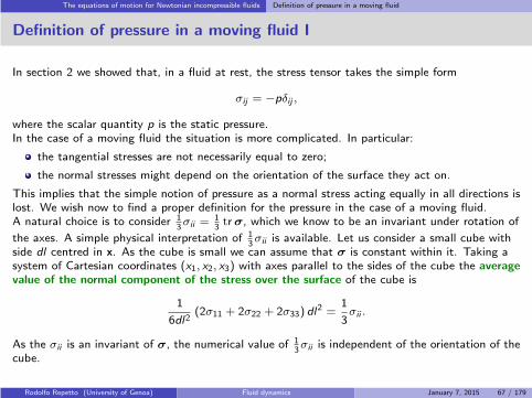
This implies that the simple notion of pressure as a normal stress acting equally in all directions islost. We wish now to find a proper definition for the pressure in the case of a moving fluid.A natural choice is to consider 1
3σii =
13trσ, which we know to be an invariant under rotation of
the axes. A simple physical interpretation of 13σii is available. Let us consider a small cube with
side dl centred in x. As the cube is small we can assume that σ is constant within it. Taking asystem of Cartesian coordinates (x1, x2, x3) with axes parallel to the sides of the cube the averagevalue of the normal component of the stress over the surface of the cube is
1
6dl2(2σ11 + 2σ22 + 2σ33) dl
2 =1
3σii .
As the σii is an invariant of σ, the numerical value of 13σii is independent of the orientation of the
cube.
Rodolfo Repetto (University of Genoa) Fluid dynamics January 7, 2015 67 / 179
The equations of motion for Newtonian incompressible fluids Definition of pressure in a moving fluid
Definition of pressure in a moving fluid II
The quantity 13σii reduces to the static fluid pressure when the fluid is at rest, and its mechanical
significance makes it an appropriate generalisation of the elementary notion of pressure.Therefore, we adopt the following definition of pressure
p = −1
3σii , or, p = −1
3trσ. (63)
Important note
Incompressible fluidsFor an incompressible fluid the pressure p is an independent, purely dynamical variable. Inthe rest of this course we will deal exclusively with incompressible fluids.
Compressible fluidsIn the case of compressible fluids we know from classical thermodynamics that we can definethe pressure of the fluid as a parameter of state, making use of an equation of state.Thermodynamical relations refer to equilibrium conditions, so we can denote thethermodynamic pressure as pe .The connection between p and pe is not trivial as p refers to dynamic conditions, in whichelements of fluid in relative motion might not be in thermodynamic equilibrium. A thoroughdiscussion of this subject can be found in Batchelor (1967). Here it suffices to say that, formost applications, is it reasonably correct to assume p = pe .
Rodolfo Repetto (University of Genoa) Fluid dynamics January 7, 2015 68 / 179
The equations of motion for Newtonian incompressible fluids Definition of pressure in a moving fluid
Definition of pressure in a moving fluid III
For the discussion to follow it is convenient to split to the stress tensor σij into an isotropic part−pδij , and a deviatoric part dij which is entirely due to fluid motion. We thus write
σij = −pδij + dij . (64)
The tensor dij accounts for tangential stresses and also normal stresses whose sum is zero.
Rodolfo Repetto (University of Genoa) Fluid dynamics January 7, 2015 69 / 179
The equations of motion for Newtonian incompressible fluids Constitutive relationship for Newtonian fluids
Constitutive relationship for Newtonian fluids I
We derive the constitutive relationship under the following assumptions.
1 The tensor d is a continuous function of ∇u.
2 If ∇u = 0 then d = 0, so that σ = −pI, i.e. the stress reduces to the stress in staticconditions.
3 The fluid is homogeneous, i.e. σ does not depend explicitly on x.
4 The fluid is isotropic, i.e. there is no preferred direction.
5 The relationship between d and ∇u is linear.
Both the tensors d and ∇u have nine scalar components. The linear assumption means that eachcomponent of d is proportional to the nine components of ∇u. Hence, in the most general casethere are 81 scalar coefficients that relate the two tensors, in the form
dij = Aijkl
∂uk
∂xl, (65)
where Aijkl is a fourth-order tensor which depends on the local state of the fluid but not directlyon the velocity distribution. Note that since dij is symmetrical so it must be Aijkl in the indices i
and j .It is convenient at this stage to recall the decomposition of the velocity gradient tensor (46) intoa symmetric and an anti-symmetric part
∂ui
∂xj= Dij +Ωij .
Rodolfo Repetto (University of Genoa) Fluid dynamics January 7, 2015 70 / 179

The equations of motion for Newtonian incompressible fluids Constitutive relationship for Newtonian fluids
Constitutive relationship for Newtonian fluids II
The assumption of isotropy of the fluid implies that the tensor Aijkl has to be isotropic. A tensoris said to be isotropic when its components are unchanged by rotation of the frame of reference.It is known from books on Cartesian tensors (e.g. Aris, 1962) that all isotropic tensors of evenorder can be written as the sum of products of δ tensors, with δ being the Kronecker tensor. Inthe case of a fourth-order tensor we can write
Aijkl = µδikδjl + µ′δilδjk + µ′′δijδkl ,
where µ, µ′ and µ′′ are scalar coefficients. Since Aijkl is symmetrical in i and j it must be
µ = µ′.
If µ = µ′ the tensor Aijkl is also symmetrical in the indices k and l . This implies that
AijklΩkl = 0,
as Ωkl is anti-symmetric. The fact that dij can not depend on Ωkl is reasonable as, on the groundof intuition, we do not expect that a motion locally consisting of a rigid body rotation inducesstress in the fluid. Note that this also implies that the assumption 2 has to be rewritten asD = 0 ⇒ d = 0.We now have that equation (65) reduces to
dij = µδikδjlDkl + µδilδjkDkl + µ′′δijδklDkl = µDij + µDji + µ′′δijDkk .
Rodolfo Repetto (University of Genoa) Fluid dynamics January 7, 2015 71 / 179

The equations of motion for Newtonian incompressible fluids Constitutive relationship for Newtonian fluids
Constitutive relationship for Newtonian fluids III
Recalling that Dkk = ∂uk∂xk
= ∇ · u, the above expression takes the form
dij = 2µDij + µ′′∇ · u δij . (66)
Finally, we recall that, by definition, dij makes no contribution to the mean normal stress,therefore
dii = (2µ+ 3µ′′)∇ · u = 0,
and, since this expression holds for any u, we find
2µ+ 3µ′′ = 0. (67)
From (64), (66) and (67) we finally obtain the constitutive equation for a Newtonian fluid in theform
σij = −pδij + 2µ
(
Dij −1
3∇ · u δij
)
, or, in vector form, σ = −pI+ 2µ
(
D− 1
3(∇ · u)I
)
.
(68)Notice that for an incompressible fluid we have ∇ · u = 0 by the continuity equation (38),therefore the constitutive law simplifies in this case to
σij = −pδij + 2µDij , or, in vector form, σ = −pI+ 2µD. (69)
Rodolfo Repetto (University of Genoa) Fluid dynamics January 7, 2015 72 / 179

The equations of motion for Newtonian incompressible fluids Constitutive relationship for Newtonian fluids
Constitutive relationship for Newtonian fluids IV
Definitions
µ is named dynamic viscosity. It has dimensions [µ] = ML−1T−1, and in the IS it ismeasured in N s m−2.
It is often convenient to define a kinematic viscosity as
ν =µ
ρ. (70)
The kinematic viscosity has dimensions [ν] = L2T−1, and in the IS is measured in m2s−1.
Inviscid fluids
A fluid is said to be inviscid or ideal if µ = 0. For an inviscid fluid the stress tensor reads
σij = −pδij , or, in vector form, σ = −pI, (71)
i.e. it takes the same form as for a fluid at rest. Note that inviscid fluids do not exist in nature.However, in some cases, real fluids can behave similarly to ideal fluids. This happens in flows inwhich viscosity plays a negligible effect.
Rodolfo Repetto (University of Genoa) Fluid dynamics January 7, 2015 73 / 179

The equations of motion for Newtonian incompressible fluids The Navier-Stokes equations
The Navier-Stokes equations
We now wish to derive the equations of motions for an incompressible Newtonian fluid. Weconsider the Cauchy equation (57) and substitute into it the constitutive relationship (69). Weobtain
ρ
(∂ui
∂t+ uj
∂ui
∂xj
)
− ρfi −∂
∂xj
(−pδij + 2µDij
)= 0. (72)
Let us consider the last term of the above expression. We can write it as
∂
∂xj
(2µDij
)= 2µ
∂
∂xj
[1
2
(∂ui
∂xj+∂uj
∂xi
)]
= µ
(
∂2ui
∂x2j
+∂2uj
∂xi∂xj
)
.
For the continuity equation, we have∂uj∂xj
= 0 ⇒ ∂∂xi
∂uj∂xj
= 0. We can then write equation (72) as
∂ui
∂t+uj
∂ui
∂xj−fi+
1
ρ
∂p
∂xi−ν ∂
2ui
∂x2j
= 0, or, in vector form,∂u
∂t+(u·∇)u−f+
1
ρ∇p−ν∇2u = 0.
(73)Recalling the definition of material derivative (27) the above equation can also be written as
Dui
Dt− fi +
1
ρ
∂p
∂xi− ν
∂2ui
∂x2j
= 0, or, in vector form,Du
Dt− f +
1
ρ∇p − ν∇2u = 0. (74)
These are called the Navier-Stokes equations and are of fundamental importance in fluidmechanics. They govern the motion of a Newtonian incompressible fluid and have to be solvedtogether with the continuity equation (38).
Rodolfo Repetto (University of Genoa) Fluid dynamics January 7, 2015 74 / 179

The equations of motion for Newtonian incompressible fluids The dynamic pressure
The dynamic pressure
We now assume that the body force acting on the fluid is gravity, therefore we set in theNavier-Stokes equation (73) f = g. When ρ is constant the pressure p in a point x of the fluidcan be written as
p = p0 + ρg · x+ P, (75)
where p0 is a constant and p0 + ρg · x is the pressure that would exist in the fluid if it was at rest.Finally, P is the part of the pressure which is associated to fluid motion and can be nameddynamic pressure. This is in fact the departure of pressure from the hydrostatic distribution.Therefore, in the Navier-Stokes equations, the term ρg −∇p can be replaced with −∇P.Thus we have:
∇ · u = 0,
∂u
∂t+ (u · ∇)u+
1
ρ∇P − ν∇2u = 0. (76)
If the Navier-Stokes equations are written in terms of the dynamic pressure gravity does notexplicitly appear in the equations.In the following whenever gravity will not be included in the Navier-Stokes this will be done withthe understanding that the pressure is the dynamic pressure (even if p will sometimes be usedinstead of P).
Rodolfo Repetto (University of Genoa) Fluid dynamics January 7, 2015 75 / 179

Initial and boundary conditions
Initial and boundary conditions
Rodolfo Repetto (University of Genoa) Fluid dynamics January 7, 2015 76 / 179

Initial and boundary conditions Initial and boundary conditions for the Navier-Stokes equations
Initial and boundary conditions for the Navier-Stokes equations
We know from the previous section that the motion of an incompressible Newtonian fluid isgoverned by the Navier-Stokes equations (73) and the continuity equation (38), namely
∂u
∂t+ (u · ∇)u− f +
1
ρ∇p − ν∇2u = 0,
∇ · u = 0.
Initial conditionsTo find an unsteady solution of the above equations, we need to prescribe initial conditions, i.e.the initial (at time t = 0) spatial distribution within the domain of pressure and velocity
p(x, 0), u(x, 0). (77)
Boundary conditionsEquations (73) and (38) have also to be solved subjected to suitable boundary conditions.We will discuss in the following the boundary conditions that have to be imposed at the interfacebetween two continuum media.We will then specify these conditions to the following, particularly relevant, cases:
solid impermeable walls;
free surfaces, e.g. interfaces between a liquid and a gas.
Rodolfo Repetto (University of Genoa) Fluid dynamics January 7, 2015 77 / 179

Initial and boundary conditions Kinematic boundary condition
Kinematic boundary condition I
The kinematic boundary condition imposes that at a boundary of the domain the normal velocityof the surface vn = v · n (with v velocity of the boundary and n unit vector normal to the surface)is equal to the normal velocity of fluid particles on the surface un = u · n. Thus we have
un = vn at the boundary. (78)
Let us determine vn. Let F (x, t) = 0 be the equation of the surface and n the normal to thissurface, defined as
n =∇F
|∇F | . (79)
Let us consider a small displacement of the surface in the time interval dt. The differential dFtaken along the direction normal to F = 0 in the time interval dt has to be equal to zero forF = 0 to still represent the equation of the surface. Thus
dF =∂F
∂ndn +
∂F
∂tdt = 0. (80)
In the above expression dn represents the displacement of the interface along the normal directionin the time interval dt. The normal component of the velocity of the surface is
vn =dn
dt. (81)
Rodolfo Repetto (University of Genoa) Fluid dynamics January 7, 2015 78 / 179

Initial and boundary conditions Kinematic boundary condition
Kinematic boundary condition II
Comparing (81) and (80) we obtain
vn = − ∂F/∂t
∂F/∂n.
Equation (79) implies n · n|∇F | = ∇F · n ⇒ |∇F | = ∂F∂n
. Therefore the above equation can bewritten as
vn = −∂F/∂t|∇F | . (82)
Substituting (82) into (78) we find
−∂F/∂t|∇F | = u · n = u · ∇F
|∇F | ,
from which, recalling (26)∂F
∂t+ u · ∇F =
DF
Dt= 0. (83)
The above equation states that the F = 0 is a material surface, i.e. it is always constituted bythe same fluid particles.
Rodolfo Repetto (University of Genoa) Fluid dynamics January 7, 2015 79 / 179

Initial and boundary conditions Continuity of the tangential component of the velocity
Continuity of the tangential component of the velocity
Given a boundary surface between two continuum media experience shows that the tangentialcomponent of the velocity is continuous across the interface. Let us denote with subscripts a
and b the two continuum media. We thus have
ua t = ub t at the boundary, (84)
where subscript t indicates the tangential components of u.
This condition can be justified by the observation that a discontinuity of the tangential velocitywould give rise to the generation of intense (infinite) stress on the surface, which would tend tosmooth out the discontinuity itself.
Rodolfo Repetto (University of Genoa) Fluid dynamics January 7, 2015 80 / 179
Initial and boundary conditions Dynamic boundary conditions
Dynamic boundary conditions
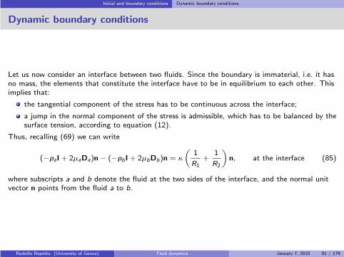
Let us now consider an interface between two fluids. Since the boundary is immaterial, i.e. it hasno mass, the elements that constitute the interface have to be in equilibrium to each other. Thisimplies that:
the tangential component of the stress has to be continuous across the interface;
a jump in the normal component of the stress is admissible, which has to be balanced by thesurface tension, according to equation (12).
Thus, recalling (69) we can write
(−paI+ 2µaDa)n− (−pbI+ 2µbDb)n = κ
(1
R1+
1
R2
)
n, at the interface (85)
where subscripts a and b denote the fluid at the two sides of the interface, and the normal unitvector n points from the fluid a to b.
Rodolfo Repetto (University of Genoa) Fluid dynamics January 7, 2015 81 / 179

Initial and boundary conditions Two relevant cases
Two relevant cases
Let us now consider two cases of particular relevance in fluid mechanics.
Fluid in contact with a solid impermeable wallWhen a fluid is in contact with a solid the boundary conditions described above take a verysimple form.
The kinematic boundary condition (83) and the conditions imposing the continuity of thetangential component of the velocity (84), imply that the velocity of the fluid at the wall uhas to be equal to the velocity of the wall uw . Thus we have
u = uw at the wall. (86)
This is named no-slip boundary condition.In the particular case in which the solid is not moving we obtain
u = 0 at the wall. (87)
There is no need to impose the dynamic boundary conditions (85), unless the problem forthe solid deformation is also solved, i.e. it is assumed that the solid is deformable.
Interface between a liquid and a gas (free surface)Typically there is no need to solve the problem for the gas motion. This has the followingconsequences.
Conditions (84) are no longer needed.
In equation (85) the stress on the gas side (b) reduces to the contribution of the pressure−pgasn.
Rodolfo Repetto (University of Genoa) Fluid dynamics January 7, 2015 82 / 179

Scaling and dimensional analysis
Scaling and dimensional analysis
Rodolfo Repetto (University of Genoa) Fluid dynamics January 7, 2015 83 / 179

Scaling and dimensional analysis Units of measurement and systems of units
Units of measurement and systems of units I
A very comprehensive book on scaling and dimensional analysis, which pays particular attentionto problems in fluid mechanics, is Barenblatt (2003). This section is based on this book.Measurement of a physical quantity is a comparison of a certain quantity with an appropriatestandard, or unit of measurement.We can divide the units for measuring physical quantities into two categories:
fundamental units;
derived units.
This has the following meaning. Let us consider a certain class of phenomena (e.g. mechanics).Let us list a number of quantities of interest and let us adopt reference values for these quantitiesas fundamental units. For instance we can choose mass, length and time standards asfundamental units. Once fundamental units have been decided upon it is possible to obtainderived units using the definition of the physical quantities. For instance, we know that density ismass per unit volume. We can therefore measure the density of a certain body by comparing itwith the density of a body that contains a unit of mass in a volume equal to the cube of a unit oflength.
Important note. Given a certain class of phenomena there is a minimum number of fundamentalunits necessary to measure all quantities within that class. However, a system of units needs notbe minimal, i.e. we may choose as fundamental units more units than we strictly need.
Definition. A set of fundamental units that is sufficient for measuring all physical properties ofthe class of phenomena under consideration is called a system of units.
Rodolfo Repetto (University of Genoa) Fluid dynamics January 7, 2015 84 / 179

Scaling and dimensional analysis Units of measurement and systems of units
Units of measurement and systems of units II
A system of units consisting of one fundamental unit (e.g. the metre) is sufficient to describegeometric objects.
Two fundamental units (e.g. the metre and the second) are sufficient to describe kinematicphenomena.
Three fundamental units (e.g. the metre, the second and the kilogram) are sufficient todescribe dynamic phenomena.
. . .
In the International System of Units SI the fundamental units for studying dynamic phenomenaare:
the kilogram kg for mass (equal to the mass of the International Prototype Kilogram,preserved at the Bureau of Weights and measures in Paris);
the metre m for length (the length of the path travelled by light in vacuum during a timeinterval of 1/299, 792, 458 s);
the second s for time (the duration of 9,192,631,770 periods of the radiation correspondingto the transition between the two hyperfine levels of the ground state of the caesium 133atom).
Rodolfo Repetto (University of Genoa) Fluid dynamics January 7, 2015 85 / 179

Scaling and dimensional analysis Units of measurement and systems of units
Units of measurement and systems of units III
Definition. Two systems of units are said to belong to the same class of systems of units if theydiffer only in the magnitude of the fundamental units, but not in their physical nature.
For instance if we choose to describe a mechanical problem adopting as fundamental units onekilometre (= 103 m), one metric ton (= 103 kg) and one hour (= 3600 s) we have a system ofunits in the same class as the SI (metre-kilogram-second).
If we regard the metre-kilogram-second as the original system in its class, then the correspondingunits on an arbitrary system in the same class are obtained as follows
unit of length = m/L, unit of mass = kg/M, unit of time = s/T , (88)
where L, M and T are positive numbers that indicate the factor by which the fundamentalunits change by passing from the original system to another system in the same class.The class of systems of units based on length, mass and time is called LMT class.
Rodolfo Repetto (University of Genoa) Fluid dynamics January 7, 2015 86 / 179

Scaling and dimensional analysis Dimension of a physical quantity
Dimension of a physical quantity I
Definition of dimensionThe function that determines the factor by which the numerical value of a physical quantitychanges upon passage from the original system of units to an arbitrary system within a given classis called dimension function or dimension of that quantity.
The dimension of a quantity F is denoted by [F ].
For example, if the units of length and time are changed by factors L and T , respectively, thenthe unit of velocity changes by a factor LT−1. According to the above definition we can say thatLT−1 is the dimension of velocity.
Definition. Quantities whose numerical value is independent of the choice of the fundamentalunits within a given class of systems of units are called dimensionless.
Important principle. In any equation with physical meaning all terms must have the samedimensions. If this was not the case an equality in one system of units would not be an equality inanother system of units within the same class.
Thus, from Newton law we find that the dimension of force ([F ]) in the LMT class is
[F ] = [m][a] = LMT−2,
with m mass and a acceleration.If, on the other hand, we adopt the LFT class (length-force-time), then the dimension of mass is[m] = L−1FT 2.
Rodolfo Repetto (University of Genoa) Fluid dynamics January 7, 2015 87 / 179
Scaling and dimensional analysis Dimension of a physical quantity
Dimension of a physical quantity II
The dimension function is a power-law monomialWe will prove this using the LMT class of systems of units. We know that the dimension of aphysical quantity a within this class depends on L, M and T only.
[a] = φ(L,M,T ).
Suppose we have chosen an original system (e.g. metre-kilogram-second). Moreover, we choosetwo further systems in the same class, say 1 and 2, so that, upon passage from the originalsystem to these new systems, the fundamental units decrease by factors L1, M1, T1 and L2, M2,T3, respectively.Let a be the numerical value of the quantity in the original system. This value will become, bydefinition of dimension, a1 = aφ(L1,M1,T1) in the first new system and a2 = aφ(L2,M2,T2) inthe second one. Thus we have
a2
a1=φ(L2,M2,T2)
φ(L1,M1,T1). (89)
All systems of units within a given class are equivalent, i.e. there are no preferred systems. Thisimplies that we may assume system 1 as the original system of the class. System 2 can then beobtained by decreasing the fundamental units by L2/L1, M2/M1 and T2/T1. This implies thatthe numerical value a2 of the considered quantity can now be written as
a2 = a1φ
(L2
L1,M2
M1,T2
T1
)
.
Rodolfo Repetto (University of Genoa) Fluid dynamics January 7, 2015 88 / 179

Scaling and dimensional analysis Dimension of a physical quantity
Dimension of a physical quantity III
Therefore we havea2
a1= φ
(L2
L1,M2
M1,T2
T1
)
. (90)
Comparing equations (89) and (90) we obtain the following functional equation for φ
φ(L2,M2,T2)
φ(L1,M1,T1)= φ
(L2
L1,M2
M1,T2
T1
)
. (91)
To solve this equation we proceed as follows. We first differentiate both sides of (91) withrespect to L2 and then set L2 = L1 = L, M2 = M1 = M and T2 = T1 = T , finding
∂
∂Lφ(L,M,T )
φ(L,M,T )=
1
L
∂
∂Lφ(1, 1, 1) =
α
L,
where α = ∂∂Lφ(1, 1, 1) is a constant. The solution of the above equation is
φ(L,M,T ) = LαC1(M,T ).
Substituting this expression into (91), we find the following functional equation for C1
C1(M2,T2)
C1(M1,T1)= C1
(M2
M1,T2
T1
)
.
Rodolfo Repetto (University of Genoa) Fluid dynamics January 7, 2015 89 / 179

Scaling and dimensional analysis Dimension of a physical quantity
Dimension of a physical quantity IV
We now differentiate this equation with respect to M2 and then set M2 = M1 = M andT2 = T1 = T .
∂
∂MC1(M,T )
C1(M,T )=
1
M
∂
∂MC1(1, 1) =
β
M,
where, again, β = ∂∂M
C1(1, 1) is a constant. Solving for C1 we obtain
C1 = MβC2(T ).
Proceeding in a similar way we finally find
C2(T ) = C3Tγ .
Thus the solution isφ = C3L
αMβTγ .
The constant C3 has to be equal to 1 as L = M = T = 1 means that the fundamental unitsremain unchanged, so that the value of the quantity a also has to remain unchanged and,therefore, it must be φ(1, 1, 1) = 1. We then finally have
φ = LαMβTγ . (92)
and we can easily verify that this is actually a solution of our original functional equation (91).
Rodolfo Repetto (University of Genoa) Fluid dynamics January 7, 2015 90 / 179
Scaling and dimensional analysis Quantities with independent dimensions
Quantities with independent dimensions I
DefinitionThe quantities a1, a2, . . . , ak are said to have independent dimensions if the monomial
aα1 aβ2 . . . a
ωk
has a dimension function equal to 1 (i.e. it is dimensionless) only forα = β = · · · = ω = 0.
ExampleLet us consider, for example, the quantities density ([ρ] = ML−3), velocity ([u] = LT−1) andforce ([f ] = MLT−2). Let us now construct the monomial Γ = ραuβ f γ . We require thismonomial to be dimensionless, thus
[Γ] = [ρ]α[u]β [f ]γ = MαL−3αLβT−βMγLγT−2γ =
= Mα+γL−3α+β+γT−β−2γ = 1.
The above equation implies
α+ γ = 0,
− 3α+ β + γ = 0,
− β − 2γ = 0.
This above system has no solution unless α = β = γ = 0. This means that the quantities ρ, uand f have independent dimensions.
Rodolfo Repetto (University of Genoa) Fluid dynamics January 7, 2015 91 / 179

Scaling and dimensional analysis Quantities with independent dimensions
Quantities with independent dimensions II
TheoremWithin a certain class of systems of units, it is always possible to pass from an original system ofunits to another system, such that any quantity, say a1, in the set of quantities a1, . . . , ak withindependent dimensions, changes its numerical value while all the others remain unchanged.
Proof
Let us consider a system of units PQ . . . . Let us consider a set of quantities with independentdimensions, whose values in a chosen original system of units are a1, . . . , ak . Upon change of thesystem of units to an arbitrary one, their numerical value becomes a′1, . . . , a
′k, such that
a′1 = a1Pα1Qβ1 . . . , . . . a′k = akP
αkQβk . . . ,
where the powers αi , βi , . . . (i = 1, . . . , k) are determined by the dimensions of each quantity.We want to find a system of units such that
a′1 = a1Pα1Qβ1 . . . , a′2 = a2, . . . a′k = ak .
We thus have a system of equations
Pα1Qβ1 · · · = A1, Pα2Qβ2 · · · = 1, . . . , PαkQβk =1.
Taking the logarithm of the above equations we obtain
α1 lnP + β1 lnQ + · · · = lnA1, α2 lnP + β2 lnQ + · · · = 0, . . . , αk lnP + βk lnQ + · · · = 0.
Rodolfo Repetto (University of Genoa) Fluid dynamics January 7, 2015 92 / 179
Scaling and dimensional analysis Quantities with independent dimensions
Quantities with independent dimensions III
This system has a solution unless the left-hand side of the first equation is a linear combination ofthe remaining ones, so that
α1 lnP + β1 lnQ + · · · = c2(α2 lnP2 + β2 lnQ + . . . ) + · · ·+ ck (αk lnPk + βk lnQ + . . . ),
with c2, . . . , ck constants. However, this implies, going back to the exponent form, that
Pα1Qβ1 · · · =(
Pα2Qβ2
)c2. . .(
PαkQβk
)ck,
or
[a1] = [a2]c2 . . . [ak ]
ck .
This contradicts the fact that a1, . . . , ak have independent dimensions and the theorem istherefore proved.
Rodolfo Repetto (University of Genoa) Fluid dynamics January 7, 2015 93 / 179

Scaling and dimensional analysis Buckingham’s Π theorem
Buckingham’s Π theorem I
Any physical study (experimental or theoretical) consists in finding one or several relationshipsbetween physical quantities in the form
a = f (a1, . . . , ak , b1, . . . , bm). (93)
In the above expression a denotes the quantity of interest. On the right-hand side of the aboveequation we have separated the physical quantities into two groups.
The k quantities a1, . . . , ak have independent dimensions;
the m quantities b1, . . . , bm can be expressed in terms of the dimensions of a1, . . . , ak .
Thus we can write
[b1] = [a1]α1 . . . [ak ]
ω1 , . . . [bm] = [a1]αm . . . [ak ]
ωm .
Note: it must be that the dimension of a is dependent on the dimensions of a1, . . . , ak , so that
[a] = [a1]α . . . [ak ]
ω .
Indeed, if a had dimensions independent from the dimensions of the variables a1, . . . , ak , for thetheorem proved above it would be possible to pass from the original system of units to anothersystem, such that the numerical value of a would change and the numerical values of a1, . . . , akand b1, . . . , bm would remain unchanged. This would indicate the need to include furtherquantities on the right-hand side of equation (93).
Rodolfo Repetto (University of Genoa) Fluid dynamics January 7, 2015 94 / 179

Scaling and dimensional analysis Buckingham’s Π theorem
Buckingham’s Π theorem II
We now introduce
Π =a
aα1 . . . aωk
,
Π1 =b1
aα11 . . . aω1
k
, . . . Πm =bm
aαm1 . . . aωm
k
.
We can thus write equation (93) as
Π =f (a1, . . . , ak , b1, . . . , bm)
aα1 . . . aωk
=f (a1, . . . , ak ,Π1a
α11 . . . aω1
k, . . . ,Πma
αm1 . . . aωm
k)
aα1 . . . aωk
,
orΠ = F(a1, . . . , ak ,Π1, . . . ,Πm).
Π and Πi (i = 1, . . . ,m) are dimensionless, therefore they don’t change their numerical valueupon changing of the system of units. Now, suppose that we change the system of units so thata1 changes its value and a2, . . . , ak remain unchanged. In the above equation a1 would be theonly variable to change and this indicates that the function F can not depend of a1. The sameargument holds for all the a1, . . . , ak variables. Therefore the above equation can be written as
Π = F(Π1, . . . ,Πm). (94)
Rodolfo Repetto (University of Genoa) Fluid dynamics January 7, 2015 95 / 179

Scaling and dimensional analysis Buckingham’s Π theorem
Buckingham’s Π theorem III
We have therefore proved that equation (93) is equivalent to equation (94), which involves onlydimensionless variables. Note, moreover, that (94) involves a smaller number of variables than(93). In particular, the number of variables involved has decreased by k, i.e. by the number ofvariables involved in (93) that have independent dimensions. This fact is of fundamentalimportance and it is one of the main reasons for which working with dimensionless quantities istypically desirable.
Rodolfo Repetto (University of Genoa) Fluid dynamics January 7, 2015 96 / 179

Scaling and dimensional analysis Dimensionless Navier-Stokes equations
Dimensionless Navier-Stokes equations I
When dealing with theoretical modelling of physical phenomena it is convenient to work withdimensionless equations. The main reasons for that are:
according to the Π theorem the number of parameters involved in the problem decreases ifone passes from a dimensional to a dimensionless formulation;
in dimensionless form (if proper scalings are adopted) it is much easier to evaluate therelative importance of different terms appearing in one equation.
Let us consider the Navier-Stokes equation and assume that the body force is gravity.Equations (73) and the continuity equation (38), can then be written as
∂u
∂t+ (u · ∇)u
︸ ︷︷ ︸
1©
−g︸︷︷︸
2©
+1
ρ∇p
︸ ︷︷ ︸
3©
−ν∇2u︸ ︷︷ ︸
4©= 0, (95)
where the vector g, representing the gravitational field, has magnitude g and is directed verticallydownwards. We recall the physical meaning of all terms:
1©: convective terms;
2©: gravity;
3©: pressure gradient;
4©: viscous term.
Rodolfo Repetto (University of Genoa) Fluid dynamics January 7, 2015 97 / 179

Scaling and dimensional analysis Dimensionless Navier-Stokes equations
Dimensionless Navier-Stokes equations II
We now wish to scale the above equation. Suppose that L is a characteristic length scale of thedomain under consideration and U a characteristic velocity. We can then introduce the followingdimensionless coordinates and variables
x∗ =x
L, u∗ =
u
U, t∗ =
t
L/U.
Above and in what follows superscript stars indicate dimensionless quantities. We still have toscale the pressure. We might consider two different situations:
1 In equation (95) 3© balances with 4©. In this case we can write
p∗ =p
ρνU/L.
2 If, on the other hand, in (95) the pressure gradient 3© balances with the convective terms 1©,we can scale the pressure as follows
p∗ =p
ρU2.
Rodolfo Repetto (University of Genoa) Fluid dynamics January 7, 2015 98 / 179

Scaling and dimensional analysis Dimensionless Navier-Stokes equations
Dimensionless Navier-Stokes equations III
Low Reynolds number flows
Let us consider the first case. Making equation (95) dimensionless using the above scales weobtain
Re
[∂u∗
∂t∗+ (u∗ · ∇∗)u∗
]
+Re
Fr2z+∇∗p∗ −∇∗2u∗ = 0, (96)
where z is the upward directed vertical unit vector.In the above equation we have defined two dimensionless parameters.
Re =UL
ν: Reynolds number. It represents the ratio between the magnitude of inertial
(convective) terms and viscous terms. It plays a fundamental role in fluid mechanics.
Fr =U√gL
: Froude number. It represents the square root of the ratio between the
magnitude of inertial (convective) terms and gravitational terms. It plays a fundamental rolewhen gravity is important, e.g. in free surface flows.
If we now consider the limit Re → 0 the dimensionless Navier-Stokes equation (96) reduces to theso called Stokes equation, i.e.
∇∗p∗ −∇∗2u∗ = 0. (97)
This equation is much simpler than the Navier-Stokes equation as it is linear. In section 10 wewill derive some analytical solutions of equation (97).
Rodolfo Repetto (University of Genoa) Fluid dynamics January 7, 2015 99 / 179

Scaling and dimensional analysis Dimensionless Navier-Stokes equations
Dimensionless Navier-Stokes equations IV
Large Reynolds number flows
Let us now consider the case in which the pressure gradient balances the convective terms. Thedimensionless Navier-Stokes equation takes the form
∂u∗
∂t∗+ (u∗ · ∇∗)u∗ +
1
Fr2z+∇∗p∗ − 1
Re∇∗2u∗ = 0. (98)
In the limit Re → ∞ the viscous term in equation (98) tends to zero. Thus we are led to thinkthat, at large values of Re, the fluid behaves as an ideal or inviscid fluid.This argument, however, has to be used with care as dropping off the viscous term from (98)means to neglect the term containing the highest order derivatives in the equation. Therefore, ifthe viscous term in (98) is neglected it is not possible to impose all boundary conditions. Toresolve this contradiction we need to assume that at the boundaries thin boundary layers form,within which viscous terms in the Navier-Stokes equations have the same magnitude asconvective terms.If boundary layers keep very thin everywhere in the flow domain the fluid out of the boundarylayers, in the core of the domain, actually behaves as if it was inviscid. This point will bediscussed in more detail in section 11.
Rodolfo Repetto (University of Genoa) Fluid dynamics January 7, 2015 100 / 179

Unidirectional flows
Unidirectional flows
Rodolfo Repetto (University of Genoa) Fluid dynamics January 7, 2015 101 / 179
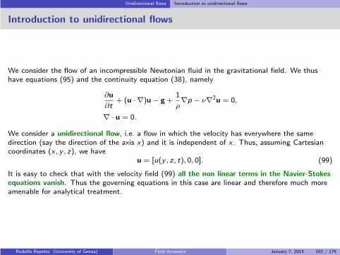
Unidirectional flows Introduction to unidirectional flows
Introduction to unidirectional flows
We consider the flow of an incompressible Newtonian fluid in the gravitational field. We thushave equations (95) and the continuity equation (38), namely
∂u
∂t+ (u · ∇)u− g +
1
ρ∇p − ν∇2u = 0,
∇ · u = 0.
We consider a unidirectional flow, i.e. a flow in which the velocity has everywhere the samedirection (say the direction of the axis x) and it is independent of x . Thus, assuming Cartesiancoordinates (x , y , z), we have
u = [u(y , z, t), 0, 0]. (99)
It is easy to check that with the velocity field (99) all the non linear terms in the Navier-Stokesequations vanish. Thus the governing equations in this case are linear and therefore much moreamenable for analytical treatment.
Rodolfo Repetto (University of Genoa) Fluid dynamics January 7, 2015 102 / 179
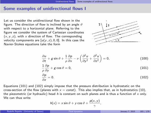
Unidirectional flows Some examples of unidirectional flows
Some examples of unidirectional flows I
Let us consider the unidirectional flow shown in thefigure. The direction of flow is inclined by an angle ϑwith respect to a horizontal plane. Referring to thefigure we consider the system of Cartesian coordinates(x , y , z), with x direction of flow. The correspondingvelocity components are [u(y , z), 0, 0]. In this case theNavier-Stokes equations take the form
∂u
∂t+ g sinϑ+
1
ρ
∂p
∂x− ν
(∂2u
∂y2+∂2u
∂z2
)
= 0, (100)
1
ρ
∂p
∂y+ g cosϑ = 0, (101)
∂p
∂z= 0. (102)
Equations (101) and (102) simply impose that the pressure distribution is hydrostatic on thecross-section of the flow (planes with x = const). This also implies that, as in hydrostatics (10),the piezometric (or hydraulic) head h is constant on such planes and is thus a function of x only.We can thus write
h(x) = x sinϑ+ y cosϑ+p(x , y)
γ,
Rodolfo Repetto (University of Genoa) Fluid dynamics January 7, 2015 103 / 179

Unidirectional flows Some examples of unidirectional flows
Some examples of unidirectional flows II
from which∂h
∂x= sinϑ+
1
γ
∂p
∂x.
We can then rewrite equation (100) as
∂u
∂t+ g
∂h
∂x− ν
(∂2u
∂y2+∂2u
∂z2
)
= 0. (103)
Since u does not depend on x it follows that also ∂h/∂x is independent of x . Hence, we can write
∂h
∂x= −j(t),
where j is function of time only. Upon substitution of j , equation (103) takes the form
∂u
∂t− gj − ν
(∂2u
∂y2+∂2u
∂z2
)
= 0. (104)
In the particular case of steady flow this simplifies to
∂2u
∂y2+∂2u
∂z2= −g
νj . (105)
Rodolfo Repetto (University of Genoa) Fluid dynamics January 7, 2015 104 / 179
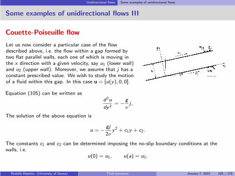
Unidirectional flows Some examples of unidirectional flows
Some examples of unidirectional flows III
Couette-Poiseuille flow
Let us now consider a particular case of the flowdescribed above, i.e. the flow within a gap formed bytwo flat parallel walls, each one of which is moving inthe x direction with a given velocity, say u1 (lower wall)and u2 (upper wall). Moreover, we assume that j has aconstant prescribed value. We wish to study the motionof a fluid within this gap. In this case u = [u(y), 0, 0].
Equation (105) can be written as
d2u
dy2= −g
νj ,
The solution of the above equation is
u = − gj
2νy2 + c1y + c2.
The constants c1 and c2 can be determined imposing the no-slip boundary conditions at thewalls, i.e.
u(0) = u1, u(a) = u2.
Rodolfo Repetto (University of Genoa) Fluid dynamics January 7, 2015 105 / 179

Unidirectional flows Some examples of unidirectional flows
Some examples of unidirectional flows IV
We finally find
u =gj
2ν(a− y)y +
u2 − u1
ay + u1. (106)
From the above solution we can easily compute the volume flux per unit length q as
q =
∫ a
0udy =
gj
12νa3 +
u2a
2+
u1a
2. (107)
We now consider a few particular cases.
Poiseuille flow: j 6= 0, u1 = u2 = 0.
In this case the flow is driven by ahydraulic head gradient alone. Thevelocity distribution (106) reduces to
u =gj
2ν(a− y)y , (108)
i.e. the velocity profile is parabolic. The maximum velocity is located at the centre of thechannel (y = a/2) and is equal to
umax =gj
8νa2,
Rodolfo Repetto (University of Genoa) Fluid dynamics January 7, 2015 106 / 179

Unidirectional flows Some examples of unidirectional flows
Some examples of unidirectional flows V
and the volume flux per unit length is
q =gj
12νa3 =
2
3umaxa.
The average velocity u is equal to 23umax.
Let us now compute the shear stress on the wall. The stress tensor has the form
σ =
0 µdu
dy0
µdu
dy0 0
0 0 0
− pI.
Thus we easily find that the tangential stress τ exerted by each wall is given by
τ = −γj2a.
Quite surprisingly the shear stress is not dependent on the viscosity of the fluid.
Rodolfo Repetto (University of Genoa) Fluid dynamics January 7, 2015 107 / 179
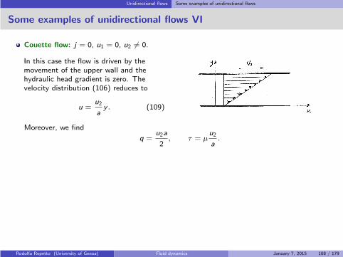
Unidirectional flows Some examples of unidirectional flows
Some examples of unidirectional flows VI
Couette flow: j = 0, u1 = 0, u2 6= 0.
In this case the flow is driven by themovement of the upper wall and thehydraulic head gradient is zero. Thevelocity distribution (106) reduces to
u =u2
ay . (109)
Moreover, we find
q =u2a
2, τ = µ
u2
a.
Rodolfo Repetto (University of Genoa) Fluid dynamics January 7, 2015 108 / 179
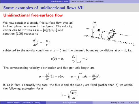
Unidirectional flows Some examples of unidirectional flows
Some examples of unidirectional flows VII
Unidirectional free-surface flow
We now consider a steady free-surface flow over aninclined plane, as shown in the figure. The velocityvector can be written as u = [u(y), 0, 0] andequation (105) reduces to
d2u
dy2= −g
νj ,
subjected to the no-slip condition at y = 0 and the dynamic boundary conditions at y = h, i.e.
u(0) = 0,du
dy
∣∣∣∣y=h
= 0.
The corresponding velocity distribution and flux per unit length are
u =gj
2ν(2h − y)y , q =
∫ h
0udy =
gj
3νh3.
If, as in fact is normally the case, the flux q and the slope j are fixed (rather than h) we obtainthe following expression for h
h = 3
√
3νq
gj.
Rodolfo Repetto (University of Genoa) Fluid dynamics January 7, 2015 109 / 179

Unidirectional flows Some examples of unidirectional flows
Some examples of unidirectional flows VIII
Axisymmetric Poiseuille flow
Let us now consider a steady, completely developed flowin a straight pipe with circular cross-section of radius R.Let the pipe axis be in the z direction and let the flowbe axisymmetric. In cylindrical coordinates (z, r , ϕ) thevelocity vector takes the form u = [u(r), 0, 0], with u
velocity component in the z direction. With thesecoordinates equation (105) takes the form
(d2
dr2+
1
r
d
dr
)
u = −gj
ν, ⇒ 1
r
d
dr
(
rdu
dr
)
= −gj
ν.
The above equation has to be solved subjected to the no-slip boundary condition at r = R and aregularity condition in r = 0.We then have
rdu
dr= − gj
2νr2 + c1, ⇒ u = − gj
4νr2 + c1 log r + c2.
Regularity at r = 0 imposes c1 = 0. Moreover, enforcing the no-slip boundary condition yields
c2 =gj
4νR2. The solution is
u =gj
4ν
(R2 − r2
). (110)
Rodolfo Repetto (University of Genoa) Fluid dynamics January 7, 2015 110 / 179

Unidirectional flows Some examples of unidirectional flows
Some examples of unidirectional flows IX
This is known as Poiseuille flow. The velocity profile is a paraboloid. The volume flux Q is givenby
Q =
∫ R
0
∫ 2π
0urdϕdr =
gjπ
8νR4. (111)
Written in cylindrical coordinates (z, r , ϕ) the stress tensor σ for this flow field takes the form
σ =
0 µdu
dr0
µdu
dr0 0
0 0 0
− pI.
We then easily compute the tangential stress τ on the wall, which reads
τ = −γj2R.
Rodolfo Repetto (University of Genoa) Fluid dynamics January 7, 2015 111 / 179
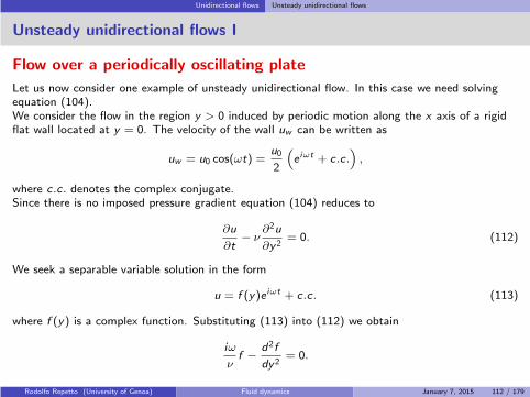
Unidirectional flows Unsteady unidirectional flows
Unsteady unidirectional flows I
Flow over a periodically oscillating plate
Let us now consider one example of unsteady unidirectional flow. In this case we need solvingequation (104).We consider the flow in the region y > 0 induced by periodic motion along the x axis of a rigidflat wall located at y = 0. The velocity of the wall uw can be written as
uw = u0 cos(ωt) =u0
2
(
e iωt + c.c.)
,
where c.c. denotes the complex conjugate.Since there is no imposed pressure gradient equation (104) reduces to
∂u
∂t− ν
∂2u
∂y2= 0. (112)
We seek a separable variable solution in the form
u = f (y)e iωt + c.c. (113)
where f (y) is a complex function. Substituting (113) into (112) we obtain
iω
νf − d2f
dy2= 0.
Rodolfo Repetto (University of Genoa) Fluid dynamics January 7, 2015 112 / 179

Unidirectional flows Unsteady unidirectional flows
Unsteady unidirectional flows II
Remembering that√i = 1√
2(1 + i), the solution of the problem is
u(y , t) =
c1 exp
− y(1 + i)√
2ν
ω
+ c2 exp
y(1 + i)√
2ν
ω
e iωt + c.c.
As the solution should not be divergent for y → ∞ we require c2 = 0. Moreover, the no-slipboundary condition at the wall imposes
c1 =u0
2.
Thus the solution of (112) is
u(y , t) =u0
2exp
− y(1 + i)√
2ν
ω
e iωt + c.c. = u0 exp
− y√
2ν
ω
cos
ωt − y
√
2ν
ω
. (114)
Rodolfo Repetto (University of Genoa) Fluid dynamics January 7, 2015 113 / 179
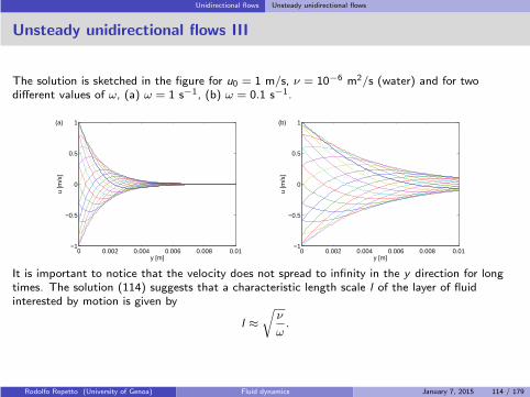
Unidirectional flows Unsteady unidirectional flows
Unsteady unidirectional flows III
The solution is sketched in the figure for u0 = 1 m/s, ν = 10−6 m2/s (water) and for twodifferent values of ω, (a) ω = 1 s−1, (b) ω = 0.1 s−1.
0 0.002 0.004 0.006 0.008 0.01−1
−0.5
0
0.5
1
y [m]
u [m
/s]
(a)
0 0.002 0.004 0.006 0.008 0.01−1
−0.5
0
0.5
1
y [m]
u [m
/s]
(b)
It is important to notice that the velocity does not spread to infinity in the y direction for longtimes. The solution (114) suggests that a characteristic length scale l of the layer of fluidinterested by motion is given by
l ≈√ν
ω.
Rodolfo Repetto (University of Genoa) Fluid dynamics January 7, 2015 114 / 179

Unidirectional flows Axisymmetric flow with circular streamlines
Axisymmetric flow with circular streamlines I
We present here another case in which the Navier-Stokes equations take a linear form. Let usconsider a flow such that all streamlines are circles centred on a common axis of symmetry.Moreover, adopting cylindrical coordinates (z, r , ϕ), we assume that the velocity, which is purelyazimuthal, only depends of the radial coordinate r and, possibly, on time t. Thus we haveu = [0, 0,w(r , t)]. We finally assume axisymmetry, so that ∂
∂ϕ≡ 0. This flow is strictly related
with unidirectional flows.
The continuity equation and the and Navier-Stokes equations in cylindrical coordinates arereported in the appendix 14 (equations (189), (190), (191) and (192)). It is immediate to verifythat, when the velocity field takes the form u = [0, 0,w(r , t)], and the flow is axisymmetric theabove equations reduce to
∂p
∂z= 0 (115)
− w2
r+
1
ρ
∂p
∂r= 0 (116)
∂w
∂t− ν
[1
r
∂
∂r
(
r∂w
∂r
)
− w
r2
]
= 0, (117)
and the continuity equation is automatically satisfied. Equation (115) implies that the pressuredoes not depend on z, and equation (116) that the radial variation of p supplies the force
Rodolfo Repetto (University of Genoa) Fluid dynamics January 7, 2015 115 / 179

Unidirectional flows Axisymmetric flow with circular streamlines
Axisymmetric flow with circular streamlines II
necessary to keep the fluid element moving along a circular path. Finally, equation (117) is linearand it is the analogous of equation (104), for a unidirectional flow.
Steady flow between two concentric rotating cylinders
Let us consider two concentric cylinders with radius R1 andR2, respectively (R2 > R1). Each of the cylinders rotateswith a given constant angular velocity (Ω1 and Ω2). The gapbetween the cylinders is filled with fluid. The flow is steadyand equation (117) reduces to
d
dr
(
rdw
dr
)
− w
r= 0,
with the boundary conditions
w = R1Ω1 (r = R1), w = R2Ω2 (r = R2).
The above equation can be rewritten as
1
r
d
dr
(
r2dw
dr− rw
)
= 0.
Rodolfo Repetto (University of Genoa) Fluid dynamics January 7, 2015 116 / 179
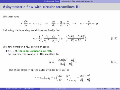
Unidirectional flows Axisymmetric flow with circular streamlines
Axisymmetric flow with circular streamlines III
We then have
r2dw
dr− rw = c1, ⇒ dw
dr=
c1
r2+
w
r, ⇒ w = − c1
2r+ c2r .
Enforcing the boundary conditions we finally find
w =1
r
(
Ω1 − Ω2
R−21 − R−2
2
)
+ r
(Ω1R
21 − Ω2R
22
R21 − R2
2
)
. (118)
We now consider a few particular cases.
Ω1 = 0, the inner cylinder is at rest.In this case the solution (118) simplifies to
w = −Ω2R22 (r
2 − R21 )
r(R21 − R2
2 ). (119)
The shear stress τ on the outer cylinder (r = R2) is
τ = σrϕ|r=R2= µ
(dw
dr− w
r
)
r=R2
=2µΩ2R
21
R21 − R2
2
,
Rodolfo Repetto (University of Genoa) Fluid dynamics January 7, 2015 117 / 179
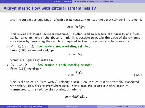
Unidirectional flows Axisymmetric flow with circular streamlines
Axisymmetric flow with circular streamlines IV
and the couple per unit length of cylinder m necessary to keep the outer cylinder in rotation is
m = 2πR22 τ.
This device (rotational cylinder rheometer) is often used to measure the viscosity of a fluid,as, by rearrangement of the above formula, it is possible to obtain the value of the dynamicviscosity µ by measuring the couple m required to keep the outer cylinder in motion.
R1 = 0, Ω1 = Ω2, flow inside a single rotating cylinder.From (118) we immediately get
w = rΩ2,
which is a rigid body rotation.
R2 → ∞, Ω2 → 0, flow around a single rotating cylinder.From (118) we obtain
w =R21Ω1
r. (120)
This is the so called “free vortex” velocity distribution. Notice that the vorticity associatedwith this velocity field is everywhere zero. In this case the couple per unit length m
transmitted to the fluid by the rotating cylinder is
m = 4πR21µΩ1,
Rodolfo Repetto (University of Genoa) Fluid dynamics January 7, 2015 118 / 179
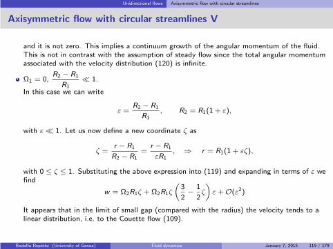
Unidirectional flows Axisymmetric flow with circular streamlines
Axisymmetric flow with circular streamlines V
and it is not zero. This implies a continuum growth of the angular momentum of the fluid.This is not in contrast with the assumption of steady flow since the total angular momentumassociated with the velocity distribution (120) is infinite.
Ω1 = 0,R2 − R1
R1≪ 1.
In this case we can write
ε =R2 − R1
R1, R2 = R1(1 + ε),
with ε≪ 1. Let us now define a new coordinate ζ as
ζ =r − R1
R2 − R1=
r − R1
εR1, ⇒ r = R1(1 + εζ),
with 0 ≤ ζ ≤ 1. Substituting the above expression into (119) and expanding in terms of ε wefind
w = Ω2R1ζ +Ω2R1ζ
(3
2− 1
2ζ
)
ε+O(ε2)
It appears that in the limit of small gap (compared with the radius) the velocity tends to alinear distribution, i.e. to the Couette flow (109).
Rodolfo Repetto (University of Genoa) Fluid dynamics January 7, 2015 119 / 179

Low Reynolds number flows
Low Reynolds number flows
Rodolfo Repetto (University of Genoa) Fluid dynamics January 7, 2015 120 / 179
Low Reynolds number flows Introduction to low Reynolds number flows
Introduction to low Reynolds number flows
In section 8 we have shown (page 99) that for low values of the Reynolds number, the equationsof motion reduce, at leading order, to the following linear equations
∇2u = ∇p, (121a)
∇ · u = 0. (121b)
The above equations, being linear, are much more amenable to analytical treatment than theoriginal Navier-Stokes equations.
In the following of this section we consider the classical solution obtained by Stokes in 1851 forthe slow flow past a sphere.
Rodolfo Repetto (University of Genoa) Fluid dynamics January 7, 2015 121 / 179
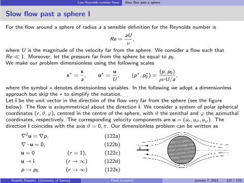
Low Reynolds number flows Slow flow past a sphere
Slow flow past a sphere I
For the flow around a sphere of radius a a sensible definition for the Reynolds number is
Re =aU
ν,
where U is the magnitude of the velocity far from the sphere. We consider a flow such thatRe ≪ 1. Moreover, let the pressure far from the sphere be equal to p0.We make our problem dimensionless using the following scales
x∗ =x
a, u∗ =
u
U, (p∗, p∗0 ) =
(p, p0)
ρνU/a,
where the symbol ∗ denotes dimensionless variables. In the following we adopt a dimensionlessapproach but skip the ∗ to simplify the notation.Let i be the unit vector in the direction of the flow very far from the sphere (see the figurebelow). The flow is axisymmetrical about the direction i. We consider a system of polar sphericalcoordinates (r , ϑ, ϕ), centred in the centre of the sphere, with ϑ the zenithal and ϕ the azimuthalcoordinates, respectively. The corresponding velocity components are u = (ur , uϑ, uϕ). Thedirection i coincides with the axis ϑ = 0, π. Our dimensionless problem can be written as
∇2u = ∇p, (122a)
∇ · u = 0, (122b)
u = 0 (r = 1), (122c)
u → i (r → ∞) (122d)
p → p0 (r → ∞) (122e)
Rodolfo Repetto (University of Genoa) Fluid dynamics January 7, 2015 122 / 179

Low Reynolds number flows Slow flow past a sphere
Slow flow past a sphere II
As a consequence of the axisymmetry of the flow we have
∂
∂ϕ= 0, uϕ = 0,
and the continuity equation takes the form
1
r2
∂
∂r
(r2ur
)+
1
r sinϑ
∂
∂ϑ(sinϑuϑ) = 0.
This allows us to introduce the so called Stokes streamfunction ψ, defined as
ur =1
r2 sinϑ
∂ψ
∂ϑ, uϑ = − 1
r sinϑ
∂ψ
∂r. (123)
Given a vector b = (br , bϑ, bϕ) we have
∇× b =r
r sinϑ
[∂
∂ϑ(bϕ sinϑ)− ∂bϑ
∂ϕ
]
+ϑ
r
[1
sinϑ
∂br
∂ϕ− ∂
∂r(rbϕ)
]
+ϕ
r
[∂
∂r(rbϑ)−
∂br
∂ϑ
]
,
with r, ϑ and ϕ unit vectors along the three coordinate directions.It is then easy to show that
u = ∇×(
0, 0,ψ
r sinϑ
)
= curl
(
0, 0,ψ
r sinϑ
)
. (124)
Rodolfo Repetto (University of Genoa) Fluid dynamics January 7, 2015 123 / 179
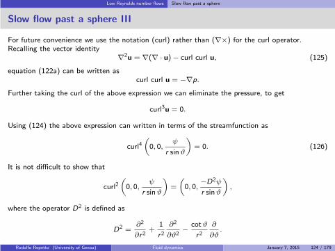
Low Reynolds number flows Slow flow past a sphere
Slow flow past a sphere III
For future convenience we use the notation (curl) rather than (∇×) for the curl operator.Recalling the vector identity
∇2u = ∇(∇ · u)− curl curl u, (125)
equation (122a) can be written ascurl curl u = −∇p.
Further taking the curl of the above expression we can eliminate the pressure, to get
curl3u = 0.
Using (124) the above expression can written in terms of the streamfunction as
curl4(
0, 0,ψ
r sinϑ
)
= 0. (126)
It is not difficult to show that
curl2(
0, 0,ψ
r sinϑ
)
=
(
0, 0,−D2ψ
r sinϑ
)
,
where the operator D2 is defined as
D2 =∂2
∂r2+
1
r2
∂2
∂ϑ2− cotϑ
r2
∂
∂ϑ.
Rodolfo Repetto (University of Genoa) Fluid dynamics January 7, 2015 124 / 179
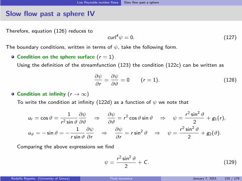
Low Reynolds number flows Slow flow past a sphere
Slow flow past a sphere IV
Therefore, equation (126) reduces tocurl4ψ = 0. (127)
The boundary conditions, written in terms of ψ, take the following form.
Condition on the sphere surface (r = 1)
Using the definition of the streamfunction (123) the condition (122c) can be written as
∂ψ
∂r=∂ψ
∂ϑ= 0 (r = 1). (128)
Condition at infinity (r → ∞)
To write the condition at infinity (122d) as a function of ψ we note that
ur = cosϑ =1
r2 sinϑ
∂ψ
∂ϑ⇒ ∂ψ
∂ϑ= r2 cosϑ sinϑ ⇒ ψ =
r2 sin2 ϑ
2+ g1(r),
uϑ = − sinϑ = − 1
r sinϑ
∂ψ
∂r⇒ ∂ψ
∂r= r sin2 ϑ ⇒ ψ =
r2 sin2 ϑ
2+ g2(ϑ).
Comparing the above expressions we find
ψ =r2 sin2 ϑ
2+ C . (129)
Rodolfo Repetto (University of Genoa) Fluid dynamics January 7, 2015 125 / 179
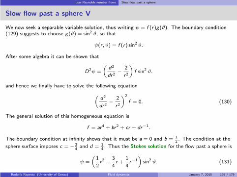
Low Reynolds number flows Slow flow past a sphere
Slow flow past a sphere V
We now seek a separable variable solution, thus writing ψ = f (r)g(ϑ). The boundary condition(129) suggests to choose g(ϑ) = sin2 ϑ, so that
ψ(r , ϑ) = f (r) sin2 ϑ.
After some algebra it can be shown that
D2ψ =
(d2
dr2− 2
r2
)
f sin2 ϑ.
and hence we finally have to solve the following equation
(d2
dr2− 2
r2
)2
f = 0. (130)
The general solution of this homogeneous equation is
f = ar4 + br2 + cr + dr−1.
The boundary condition at infinity shows that it must be a = 0 and b = 12. The condition at the
sphere surface imposes c = − 34and d = 1
4. Thus the Stokes solution for the flow past a sphere is
ψ =
(1
2r2 − 3
4r +
1
4r−1
)
sin2 ϑ. (131)
Rodolfo Repetto (University of Genoa) Fluid dynamics January 7, 2015 126 / 179
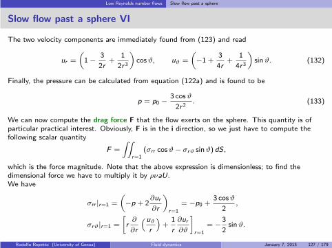
Low Reynolds number flows Slow flow past a sphere
Slow flow past a sphere VI
The two velocity components are immediately found from (123) and read
ur =
(
1− 3
2r+
1
2r3
)
cosϑ, uϑ =
(
−1 +3
4r+
1
4r3
)
sinϑ. (132)
Finally, the pressure can be calculated from equation (122a) and is found to be
p = p0 −3 cosϑ
2r2. (133)
We can now compute the drag force F that the flow exerts on the sphere. This quantity is ofparticular practical interest. Obviously, F is in the i direction, so we just have to compute thefollowing scalar quantity
F =
∫∫
r=1(σrr cosϑ− σrϑ sinϑ) dS ,
which is the force magnitude. Note that the above expression is dimensionless; to find thedimensional force we have to multiply it by ρνaU.We have
σrr |r=1 =
(
−p + 2∂ur
∂r
)
r=1
= −p0 +3 cosϑ
2,
σrϑ|r=1 =
[
r∂
∂r
(uϑ
r
)
+1
r
∂ur
∂ϑ
]
r=1
= −3
2sinϑ.
Rodolfo Repetto (University of Genoa) Fluid dynamics January 7, 2015 127 / 179
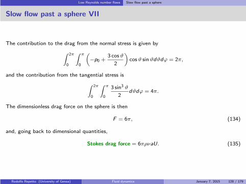
Low Reynolds number flows Slow flow past a sphere
Slow flow past a sphere VII
The contribution to the drag from the normal stress is given by
∫ 2π
0
∫ π
0
(
−p0 +3 cosϑ
2
)
cosϑ sinϑdϑdϕ = 2π,
and the contribution from the tangential stress is
∫ 2π
0
∫ π
0
3 sin3 ϑ
2dϑdϕ = 4π.
The dimensionless drag force on the sphere is then
F = 6π, (134)
and, going back to dimensional quantities,
Stokes drag force = 6πρνaU. (135)
Rodolfo Repetto (University of Genoa) Fluid dynamics January 7, 2015 128 / 179

Low Reynolds number flows Lubrication Theory
Lubrication theory I
This technique provides a good approximation to the real solution when the domain of the fluidis long and thin.
For simplicity let us assume that the flow is two dimensional (all derivatives with respect to thethird coordinate, say z, may be neglected) and that the height of the domain is h(x) and a typicalstreamwise length is L.
The fluid velocity at the vessel walls is zero (no-slip condition) but the fluid velocity at the surfaceof the cell equals the cell velocity (U). Therefore changes in the x-velocity u are on the order ofU, that is |∆u| ∼ U, and |∂u/∂y | ∼ |∆u/∆y | ∼ U/h0, where h0 is a characteristic value of h(x).
The change in fluid velocity as we move through a distance L in the x-direction is likely to be atmost U, and therefore |∂u/∂x | ∼ U/L. The continuity equation,
∂u
∂x+∂v
∂y= 0,
implies that |∂v/∂y | ∼ U/L; hence |∆v | ∼ h0U/L.
ScalingWe nondimensionalise
x = Lx∗, y = h0y∗, h(x) = h0h
∗(x∗), u = Uu∗, v = h0Uv∗/L, p = p0p
∗,
where p0 is an appropriate scale for the pressure (to be chosen). Note that x∗, y∗, u∗, v∗ and p∗
are all order 1. (Note also that the flow has a low Reynolds number, so we expect to scale thepressure gradient with the viscous terms.)
Rodolfo Repetto (University of Genoa) Fluid dynamics January 7, 2015 129 / 179

Low Reynolds number flows Lubrication Theory
Lubrication theory II
Neglecting gravity and assuming a steady solution, the nondimensional governing equations are
ǫ2Re
(
u∗∂u∗
∂x∗+ v∗ ∂u
∗
∂y∗
)
=− h20p0
µUL
∂p∗
∂x∗+ ǫ2
∂2u∗
∂x∗2+∂2u∗
∂y∗2, (136)
ǫ3Re
(
u∗∂v∗
∂x∗+ v∗ ∂v
∗
∂y∗
)
=− h20p0
ǫµUL
∂p∗
∂y∗+ ǫ3
∂2v∗
∂x∗2+ ǫ
∂2v∗
∂y∗2, (137)
∂u∗
∂x∗+∂v∗
∂y∗=0, (138)
where ǫ = h0/L ≪ 1 and Re = UL/ν.We may immediately cancel the viscous terms that have a repeated x∗-derivative since they aremuch smaller than the viscous terms with a repeated y∗-derivative. Balancing the pressurederivative and viscous terms in the x-component equation (136) leads to the scalingp0 = µUL/h20.Multiplying equation (137) by ǫ and simplifying, equations (136) and (137) can be written as
ǫ2Re
(
u∗∂u∗
∂x∗+ v∗ ∂u
∗
∂y∗
)
=− ∂p∗
∂x∗+∂2u∗
∂y∗2, (139)
0 =− ∂p∗
∂y∗, (140)
where we have neglected terms of order ǫ2 and terms of order ǫ3Re relative to theleading-order terms.
Rodolfo Repetto (University of Genoa) Fluid dynamics January 7, 2015 130 / 179

Low Reynolds number flows Lubrication Theory
Lubrication theory III
Solution procedure
The quantity ǫ2Re is called the reduced Reynolds number. We assume it is not too large,which places an upper bound on the possible flux.
We may immediately solve (140) to find that the pressure is a function of x∗ only, that is,the pressure is constant over the height of the gap.
The governing equations are thus (139) and (138), where p∗ is a function of x∗ only andthese must be solved subject to no-slip boundary conditions for u∗ at the walls.
Rodolfo Repetto (University of Genoa) Fluid dynamics January 7, 2015 131 / 179

Low Reynolds number flows Lubrication Theory
Lubrication theory IV
Series expansion for small reduced Reynolds number
In the case that the reduced Reynolds number is small, ǫ2Re ≪ 1 we can use a series expansionmethod to find the velocity, by setting
u∗ =u∗0 + ǫ2Re u∗1 +(ǫ2Re
)2u∗2 + . . . ,
v∗ =v∗0 + ǫ2Re v∗
1 +(ǫ2Re
)2v∗2 + . . . ,
p∗ =p∗0 + ǫ2Re p∗1 +(ǫ2Re
)2p∗2 + . . . .
noting that all the p∗i ’s are independent of y , and then solving for u∗0 (from equation (139)), v∗0
(from equation (138)), u∗1 (from equation (139)), v∗1 (from equation (138)), etc in that order. An
equation for the pressure can be obtained by integrating the continuity equation over the gapheight.
In many cases it is sufficiently accurate to find just the first terms u∗0 and v∗0 (or even just u∗0 ).
GeneralisationNote that we could generalise this approach to include:
dependence upon the third spatial dimension;
time-dependence of the solution;
gravity;
. . . .
Rodolfo Repetto (University of Genoa) Fluid dynamics January 7, 2015 132 / 179

Low Reynolds number flows Lubrication Theory
Lubrication theory V
Example of solution
We consider the domain shown in the figure. For simplicity, we assume two-dimensional flow. Wewish to solve the flow in the gap 0 ≤ y ≤ h(x), with 0 ≤ x ≤ L.The flowis subject to the following boundary conditions:
no-slip at y = 0 and y = h(x);
given
flux per unit length F =∫ h00 udy at x = 0;
given pressure p = 0 at x = L.
We assume that h0 = h(0) is a typical value ofthe thickness of the domain in the y -direction andassume that ǫ = h0/L ≪ 1. We can, therefore, apply the lubrication theory.We scale the variables as follows
x∗ =x
L, y∗ =
y
h0, u∗ =
u
U, v∗ =
v
ǫU,
with U = F/h0.
Rodolfo Repetto (University of Genoa) Fluid dynamics January 7, 2015 133 / 179

Low Reynolds number flows Lubrication Theory
Lubrication theory VI
Assuming that ǫ2Re ≪ 1, we need to solve the following dimensionless equations (see equations(139), (140) and (138))
∂2u∗
∂y∗2− ∂p∗
∂x∗= 0, (141)
∂p∗
∂y∗= 0, (142)
∂u∗
∂x∗+∂v∗
∂y∗= 0, (143)
subject to the boundary conditions
u∗ = v∗ = 0 (y∗ = 0), (144)
u∗ = v∗ = 0 [y∗ = h∗(x∗)], (145)∫ 1
0u∗dy∗ = 1 (x∗ = 0), (146)
p∗ = 0 (x∗ = 1). (147)
Rodolfo Repetto (University of Genoa) Fluid dynamics January 7, 2015 134 / 179
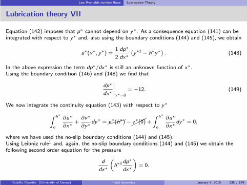
Low Reynolds number flows Lubrication Theory
Lubrication theory VII
Equation (142) imposes that p∗ cannot depend on y∗. As a consequence equation (141) can beintegrated with respect to y∗ and, also using the boundary conditions (144) and (145), we obtain
u∗(x∗, y∗) =1
2
dp∗
dx∗
(y∗2 − h∗y∗) . (148)
In the above expression the term dp∗/dx∗ is still an unknown function of x∗.Using the boundary condition (146) and (148) we find that
dp∗
dx∗
∣∣∣∣x∗=0
= −12. (149)
We now integrate the continuity equation (143) with respect to y∗
∫ h∗
o
∂u∗
∂x∗+∂v∗
∂y∗dy∗ =v∗(h∗)−
v∗(0) +
∫ h∗
o
∂u∗
∂x∗dy∗ = 0,
where we have used the no-slip boundary conditions (144) and (145).Using Leibniz rule1 and, again, the no-slip boundary conditions (144) and (145) we obtain thefollowing second order equation for the pressure
d
dx∗
(
h∗3dp∗
dx∗
)
= 0.
Rodolfo Repetto (University of Genoa) Fluid dynamics January 7, 2015 135 / 179
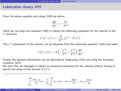
Low Reynolds number flows Lubrication Theory
Lubrication theory VIII
From the above equation and using (149) we obtain
dp∗
dx∗= − 12
h∗3,
which we can plug into equation (148) to obtain the following expression for the velocity in thex∗-direction
u∗(x∗, y∗) = − 6
h∗3
(y∗2 − h∗y∗) .
The y∗-component of the velocity can be obtained from the continuity equation (143) and reads
v∗(x∗, y∗) = −6
(
− y∗3
h∗4+
y∗2
h∗3
)dh∗
dx∗.
Finally, the pressure distribution can be obtained by integrating (129) and using the boundarycondition (147).We note that we managed to obtain an analytical expression for the velocity without having tospecify the shape of the domain h∗(x∗).
1
b(z)∫
a(z)
∂f (x, z)
∂zdx =
∂
∂z
b(z)∫
a(z)
f (x, z)dx − f (b, z)∂b(z)
∂z+ f (a, z)
∂a(z)
∂z.
Rodolfo Repetto (University of Genoa) Fluid dynamics January 7, 2015 136 / 179
High Reynolds number flows
High Reynolds number flows
Rodolfo Repetto (University of Genoa) Fluid dynamics January 7, 2015 137 / 179
High Reynolds number flows The Bernoulli theorem
The Bernoulli theorem I
As a first tool to study high Reynolds number flows we introduce the Bernoulli theorem. As itwill appear in the following, provided that some assumptions hold, this theorem is a very powerfultool to solve practical problems by very simple means.
Let us recall the following vector identity
u× (∇× u) =1
2∇(u · u)− (u · ∇)u. (150)
Plugging it into the Navier-Stokes equation, we can rewrite (73) as
∂u
∂t− u× ω − f +∇
(p
ρ+
1
2|u|2)
− ν∇2u = 0, (151)
where ω is the vorticity defined by (51).Let us now assume that f is conservative. We can then write f = −∇Ψ, with Ψ scalar potentialfunction. Let, moreover assume that the flow is steady, so that ∂u/∂t = 0. Under the aboveassumptions we can write (151) as
∇H′ = u× ω + ν∇2u,
where we have defined
H′ =1
2|u|2 +Ψ+
p
ρ. (152)
Rodolfo Repetto (University of Genoa) Fluid dynamics January 7, 2015 138 / 179

High Reynolds number flows The Bernoulli theorem
The Bernoulli theorem II
If the fluid is inviscid (or, more realistically, if viscosity plays a negligible role in the flow underconsideration), we have
∇H′ = u× ω.
Projecting the above equation in the direction of flow we obtain
u · ∇H′ = 0.
The above equation implies that H′ is constant along the streamlines, which is a remarkablysimple result.
Particular case: gravitational body force field
In the particular case in which the body force is gravity we have
Ψ = gz,
with z a vertical and upwards directed coordinate. In this case we then have
H′ =1
2|u|2 + p
ρ+ gz.
It is customary, in fluid mechanics and hydraulics to work with the quantity H = H′/g , so that
H = z +p
γ+
|u|22g
. (153)
H is named total head and it represents the total mechanical energy per unit weight of the fluid.Note that if the fluid is at rest H reduces to the pressure head, defined in section 3.
Rodolfo Repetto (University of Genoa) Fluid dynamics January 7, 2015 139 / 179

High Reynolds number flows The Bernoulli theorem
The Bernoulli theorem III
Bernoulli theorem can be stated as follows. If the following conditions are satisfied:
the fluid is incompressible,
the body force is gravity (or more in general it is conservative),
the flow is steady,
the effects of viscosity are negligible,
then the total head H is constant along streamlines. Note that the value of H can differ fromone streamline to another.
Rodolfo Repetto (University of Genoa) Fluid dynamics January 7, 2015 140 / 179
High Reynolds number flows Vorticity equation and vorticity production
Vorticity equation and vorticity production I
Vorticity equationWe wish to determine an equation for the vorticity ω = ∇× u, see equation (51). Theimportance of the vorticity equation for studying large Reynolds number flows will become clearin the following.We take the curl of the Navier-Stokes equation (73), in which we assume that the body forcefield is conservative, so that we can write f = −∇Ψ. We then obtain
∇×[∂u
∂t+∇
(u · u2
)
− u× ω +∇Ψ+1
ρ∇p − ν∇2u
]
= 0. (154)
In the above equation we have used the vector identity (150).As the curl of a gradient is zero the second, fourth and fifth terms in equation (154) vanish.Therefore we can write, using the index notation,
ǫijk∂
∂xj
∂uk
∂t− ǫijk
[∂
∂xj(ǫklmulωm)
]
− νǫijk∂
∂xj
∂2uk
∂x2l
= 0,
or∂ωi
∂t− ∂
∂xj(ǫijkǫklmulωm)− ν
∂2ωi
∂x2l
= 0.
We note that by definition of the alternating tensor we have ǫijk = ǫkij . Moreover, the followingformula holds
ǫkij ǫklm = δilδjm − δimδjl . (155)
Rodolfo Repetto (University of Genoa) Fluid dynamics January 7, 2015 141 / 179
High Reynolds number flows Vorticity equation and vorticity production
Vorticity equation and vorticity production II
Therefore, we can write∂ωi
∂t− ∂
∂xj(uiωj − ujωi )− ν
∂2ωi
∂x2j
= 0.
From the continuity equation we have that ∂uj/∂xj = 0. Moreover, the divergence of a curl iszero, and therefore, ∂ωj/∂xj = 0. The above equation then simplifies to
∂ωi
∂t+ uj
∂ωi
∂xj− ωj
∂ui
∂xj− ν
∂2ωi
∂x2j
= 0, (156)
or, in vector form,∂ω
∂t+ (u · ∇)ω − (ω · ∇)u− ν∇2ω = 0. (157)
This equation is called vorticity equation and it is of fundamental importance in fluid mechanics.
The first and second terms in equation (157) represent advective transport of vorticity.
The last term represents viscous (diffusive) transport of vorticity.
The third term does not have a counterpart in the Navier-Stokes equations. It accounts forchanges of vorticity due to deformation of material elements of the fluid.
Note, that pressure and body force do not appear in the vorticity equation.
Rodolfo Repetto (University of Genoa) Fluid dynamics January 7, 2015 142 / 179
High Reynolds number flows Vorticity equation and vorticity production
Vorticity equation and vorticity production III
Changes of vorticity in a volume V
Let us now study how the amount of vorticity changes in a fluid volume V . A suitable measure ofthe amount of vorticity is the enstrophy, defined as (ω · ω)/2. Multiplying equation (156) by ωi
we obtain∂
∂t
(
ω2i
2
)
+ uj∂
∂xj
(
ω2i
2
)
− ωiωj
∂ui
∂xj− νωi
∂2ωi
∂x2j
= 0.
After some algebraic manipulation this can be written as
∂
∂t
(
ω2i
2
)
+ uj∂
∂xj
(
ω2i
2
)
− ωiωj
∂ui
∂xj− ν
[
∂2
∂x2j
(
ω2i
2
)
−(∂ωi
∂xj
)2]
= 0.
Taking the integral of the above expression over a material volume V and applying the Reynoldstransport theorem we obtain
D
Dt
∫∫∫
V
(
ω2i
2
)
dV =
∫∫∫
V
ωiωj
∂ui
∂xjdV +
∫∫∫
V
ν∂2
∂x2j
(
ω2i
2
)
dV −∫∫∫
V
ν
(∂ωi
∂xj
)2
dV . (158)
The term on the left hand side represents the time variation of the enstrophy associated withthe volume V .
Rodolfo Repetto (University of Genoa) Fluid dynamics January 7, 2015 143 / 179

High Reynolds number flows Vorticity equation and vorticity production
Vorticity equation and vorticity production IV
The first term on the right hand side induces changes of vorticity in V , as a response to thevelocity distribution. Note, however, that this is not a source term: if at some time thevorticity within V is zero this term can not produce new vorticity.
Making use of Gauss theorem the second term on the right hand side can be transformedinto a flux term across the surface S bounding V as follows
∫∫∫
V
ν∂2
∂x2j
(
ω2i
2
)
dV =ν
2
∫∫
S
nj∂
∂xjω2i dS .
Therefore it does not produce nor dissipate vorticity.
Finally the last term represents viscous dissipation of vorticity and always contributes todecrease the amount of vorticity within the volume V .
Equation (158) shows that the vorticity can not be generated within a body of fluid. It thenfollows that vorticity can only be generated at the boundary of the domain.A typical source of vorticity is, for instance, the no-slip condition (86), which holds incorrespondence of solid walls.
Rodolfo Repetto (University of Genoa) Fluid dynamics January 7, 2015 144 / 179

High Reynolds number flows Vorticity equation and vorticity production
Vorticity equation and vorticity production V
Generation of vorticity due to an impulsively started solid body
To understand the generation and transport of vorticity let us consider an example: a fluidoccupying an infinite region and initially (at time t = 0) at rest is set in motion by a solid bodyimmersed in the fluid that, at t = 0, impulsively starts moving with velocity U. Suppose that westudy this flow in a frame moving with the solid body.We can think that the development of motion in the fluid takes place in three different phases.
1 At the initial time (t = 0) the fluid starts moving and the flow is irrotational, i.e. thevorticity is zero everywhere. In fact the vorticity is initially confined in an infinitesimally thinlayer at the wall and, within that layer the vorticity is theoretically infinite.
2 For t > 0 the vorticity starts be transported away from the wall. Transport occurs both forviscous diffusion and advection. If diffusion was the only transport mechanism the thicknessof the boundary layer in which the flow is not irrotational would be of order
√νt at time t.
At the very initial stage advection is expected to have a relatively small effect as, initially, thenormal component of the relative velocity of the fluid with respect to the wall is expected tobe small. Thus for small times the thickness of the boundary layer will be of the order of√νt.
Rodolfo Repetto (University of Genoa) Fluid dynamics January 7, 2015 145 / 179
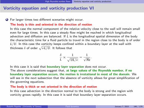
High Reynolds number flows Vorticity equation and vorticity production
Vorticity equation and vorticity production VI
3 For larger times two different scenarios might occur.
The body is thin and oriented in the direction of motion
In this case the normal component of the relative velocity close to the wall will remain smalleven for large times. In this case a steady flow might be reached in which longitudinaladvection and diffusion are balanced. If L is the longitudinal spatial dimension of the bodythe characteristic time for a fluid particle to travel in the region close to the body is of orderL/U. In this case the vorticity keeps confined within a boundary layer at the wall with
thickness δ of order√νL/U. It follows that
δ
L∝ 1√
UL/ν=
1√Re.
In this case it is said that boundary layer separation does not occur.The above considerations suggest that, at large values of the Reynolds number, if noboundary layer separation occurs, the motion is irrotational in most of the domain. Wewill see in the next subsection that the absence of vorticity allows for great simplification ofthe governing equations.
The body is thick or not oriented in the direction of motion
In this case advection in the direction normal to the body is strong and the region withvorticity grows rapidly. In this case it is said that boundary layer separation occurs.
Rodolfo Repetto (University of Genoa) Fluid dynamics January 7, 2015 146 / 179

High Reynolds number flows Irrotational flows
Irrotational flows I
Potential function of the velocityWe have seen in the last section that at large values of the Reynolds number it might happenthat in most of the flow domain motion remains irrotational. We now wish to study if theassumptions of
incompressible fluid, and
irrotational flow,
i.e.∇ · u = 0, ∇× u = 0. (159)
allow for any simplifications of the problem. Note that the conditions (159) are of purelykinematic nature even if they are consequence of the dynamic behaviour of the fluid.
Let us consider a closed reducible curve C and let us take the line integral of the velocity alongthis curve. We have, by Stokes theorem,
∮
C
u · dx =
∫∫
S
(∇× u) · ndS =
∫∫
S
ω · ndS = 0.
We now consider any two points, say O and P, on C . They split C into two curves, C1 and C2,with both C1 and C2 joining O to P. We then have
∮
C1
u · dx =
∮
C2
u · dx.
Rodolfo Repetto (University of Genoa) Fluid dynamics January 7, 2015 147 / 179
High Reynolds number flows Irrotational flows
Irrotational flows II
This implies that the integral between O and P does not depend on the path of integration butonly on the starting and ending points. We can then define a potential function φ(x) of thevelocity field, such that
φ(x) = φ(x0) +
∫ P
0u · dx. (160)
Equation (160) implies that we can write
u = ∇φ. (161)
If we recall the continuity equation for an incompressible fluid, i.e. ∇ · u = 0, and plug (161) intoit we find
∇2φ = 0, (162)
which implies that the potential function φ has to be harmonic. In other words the velocitypotential function satisfies the Laplace equation. If we solve the problem for the function φ wecan then easily find the velocity u using equation (161).It is clear that the mathematical problem for an irrotational flow is much easier than that for arotational flow, for the following main reasons:
equation (162) is linear, whereas the Navier-Stokes equations are nonlinear;
in the case of an irrotational flow it is sufficient to solve the problem for a scalar functionrather than a vector function;
Rodolfo Repetto (University of Genoa) Fluid dynamics January 7, 2015 148 / 179
High Reynolds number flows Irrotational flows
Irrotational flows III
the problem for the pressure is decoupled from the problem for the velocity field. How tocompute the pressure in an irrotational flow will be discussed in the following.
Owing to the properties of equation (162) we can state that the velocity distribution has thefollowing properties.
As equation (162) is elliptic the solution for φ and all its derivatives is smooth except, atmost, on the boundary.
The function φ is single-valued if the considered domain is simply connected.
In the following we will only consider the case of simply connected regions.
Conditions for φ to be uniquely determinedLet us now consider the boundary conditions we need to impose for the solution for φ to beunique. We first note that the following vector identity holds
∇ · (φu) = φ∇ · u+ u · ∇φ = u · u,
from which we can write, also using the divergence theorem,
∫∫∫
V
u · udV =
∫∫∫
V
∇ · (φu)dV =
∫∫
S
φu · ndS . (163)
Rodolfo Repetto (University of Genoa) Fluid dynamics January 7, 2015 149 / 179

High Reynolds number flows Irrotational flows
Irrotational flows IV
Let u1 = ∇φ1 and u2 = ∇φ2 be two solutions of equation (162). The difference (u1 − u2) is alsoa solution, owing to the linearity of the equation. Recalling equation (163) we can write
∫∫∫
V
|u1 − u2|2 dV =
∫∫
S
(φ1 − φ2)(u1 − u2) · ndS .
The above expression shows that u1 and u2 coincide if
(u1 − u2) · n = 0 on the boundary S , i.e. if the normal components of the velocity are thesame (Neumann conditions);
or if φ1 = φ2 on S (Dirichlet conditions);
of if (u1 − u2) · n = 0 on a portion of S and φ1 = φ2 on the remaining part of S .
It is important to notice that for an irrotational flow it is not possible to impose the no-slipcondition at solid walls as only the normal component of the velocity is required. However, closeto rigid walls a boundary layer exists, in which the flow is rotational. To determine the flow in theboundary layer the Navier-Stokes equations have to be solved.
Rodolfo Repetto (University of Genoa) Fluid dynamics January 7, 2015 150 / 179
High Reynolds number flows Bernoulli equation for irrotational flows
Bernoulli equation for irrotational flows I
We have shown that the potential function φ can be obtained by using the irrotationality of theflow and the continuity equation. We now consider the momentum equation (Navier-Stokesequation) and study how it simplifies in the case of irrotational flow. We anticipate that the useof the momentum equation will allow us to determine the pressure.
Recalling the vector identities (125) and (150) the Navier-Stokes equation (73) can then bewritten as
∂u
∂t+∇
( |u|22
)
− u× ω +1
ρ∇p − f = 0
Assuming that the the body force field is conservative we can write f = −∇Ψ. If the flow isirrotational we have ω = 0 and u = ∇φ. Thus we can write
∇(∂φ
∂t+
|u|22
+p
ρ+Ψ
)
= 0.
This equation can be solved to get
∂φ
∂t+
|u|22
+p
ρ+Ψ = F (t). (164)
Notice that, without loss of generality, we can introduce a function φ such that
φ = φ−∫
Fdt,
Rodolfo Repetto (University of Genoa) Fluid dynamics January 7, 2015 151 / 179
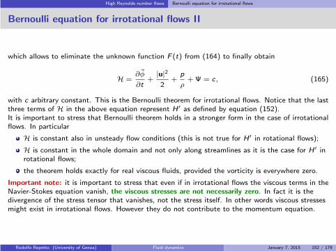
High Reynolds number flows Bernoulli equation for irrotational flows
Bernoulli equation for irrotational flows II
which allows to eliminate the unknown function F (t) from (164) to finally obtain
H =∂φ
∂t+
|u|22
+p
ρ+Ψ = c, (165)
with c arbitrary constant. This is the Bernoulli theorem for irrotational flows. Notice that the lastthree terms of H in the above equation represent H′ as defined by equation (152).It is important to stress that Bernoulli theorem holds in a stronger form in the case of irrotationalflows. In particular
H is constant also in unsteady flow conditions (this is not true for H′ in rotational flows);
H is constant in the whole domain and not only along streamlines as it is the case for H′ inrotational flows;
the theorem holds exactly for real viscous fluids, provided the vorticity is everywhere zero.
Important note: it is important to stress that even if in irrotational flows the viscous terms in theNavier-Stokes equation vanish, the viscous stresses are not necessarily zero. In fact it is thedivergence of the stress tensor that vanishes, not the stress itself. In other words viscous stressesmight exist in irrotational flows. However they do not contribute to the momentum equation.
Rodolfo Repetto (University of Genoa) Fluid dynamics January 7, 2015 152 / 179

Introduction to numerical methods
Introduction to numerical methods
Rodolfo Repetto (University of Genoa) Fluid dynamics January 7, 2015 153 / 179

Introduction to numerical methods What is computational fluid dynamics
Computational fluid dynamics (CFD)
The equations governing fluid flow have been derived more than a century ago and have beenproved to very accurately describe real phenomena.However, as discussed in previous chapters, these equations can be solved analytically only inextremely specific cases (i.e. unidirectional flows, see chapter 9).One has therefore to resort to approximate solutions of the equations governing fluid flows. Thisis where computational fluid dynamics (CFD) comes into play. With the CFD approach one seeksa numerical solution of the governing equations. This means that the original set of partialdifferential equations is discretised and transformed into a set of algebraic equations that can besolved on a computer.
Some referencesNumerous textbooks of numerical methods and computational fluid dynamics exist. The followingbooks are good references for numerical methods in fluid mechanics:
Ferziger and Peric (2002),
Pletcher et al. (2012),
Versteeg and Malalasekera (2007),
Toro (2009).
Rodolfo Repetto (University of Genoa) Fluid dynamics January 7, 2015 154 / 179

Introduction to numerical methods A short introduction to numerical solutions of differential equations
Components of a method for a numerical solution I
Mathematical modelThe starting point of a numerical solution is a mathematical model that describes a physicalphenomenon. This may consist in a set of ordinary (ODE) or partial (PDE) differential equations.For instance, in the case of flow of a viscous, incompressible fluid the mathematical modelconsists in the Navier-Stokes equations (73) and continuity equation (38). For particularapplications (such as flows at low or large values of the Reynolds number) these equations canpossibly be simplified, as it was discussed in the previous chapters.
Discretisation methodThe second step consists in the choice of a discretisation method, i.e. a method for transformingthe differential operators appearing in the mathematical model into algebraic expressions. Thismeans that the unknowns have to be evaluated at a certain number of discrete points in spaceand/or time. This discretisation procedure can be performed in various ways. The three mostimportant methods are:
finite difference method;
finite volume method;
finite element method.
Each of the methods have its own pros and cons. They all should lead to the same solution in thelimit of infinitely fine computational grid.In the following a short introduction to the finite difference method will be given.
Rodolfo Repetto (University of Genoa) Fluid dynamics January 7, 2015 155 / 179

Introduction to numerical methods A short introduction to numerical solutions of differential equations
Components of a method for a numerical solution II
Numerical gridThe locations at which the numerical solution is computed define the computational grid ormesh, which is, therefore, a discrete representation on the computational domain (including timefor unsteady problems).
Structured meshes
Regular or structured grids consist of families of grid lines with the property that members ofa single family do not cross each other and cross each member of the other families onlyonce (Ferziger and Peric, 2002). This implies that grid points can be numberedconsecutively. A Cartesian grid is obviously structured, but structured grids can have morecomplicated shapes. An example is given in the figure below.
Rodolfo Repetto (University of Genoa) Fluid dynamics January 7, 2015 156 / 179

Introduction to numerical methods A short introduction to numerical solutions of differential equations
Components of a method for a numerical solution III
Unstructured meshes
For very complex geometries structured meshes might nor be suitable. In this case it isbetter to rely on unstructured grids, as the one shown in the figure below, which can beadapted to any shape of the computational domain. The elements or control volumes canhave any shape and there are no restrictions on the number of neighbour volumes. Of coursethe flexibility obtained using unstructured meshes comes to the cost of having an irregulardata structure. Since the nodes cannot be numbered consequently node location andneighbour connections have to be explicitly specified.
Rodolfo Repetto (University of Genoa) Fluid dynamics January 7, 2015 157 / 179

Introduction to numerical methods A short introduction to numerical solutions of differential equations
Properties of numerical methods I
ConsistencyA numerical method is said to be consistent if the discretisation of the differential operators tendsto become exact as the grid spacing tends to zero. The difference between the discretisedequation and the exact one is called truncation error.Usually the truncation error is proportional to a power of the grid spacing, say ∆x . If thetruncation error is of order (∆x)n it is said that the numerical method is an nth-orderapproximation.
StabilityA numerical method is stable if it does not magnify the errors in the course of the numericalsolution procedure. Investigating the stability of a numerical method can be difficult, especially inthe case of nonlinear equations.
ConvergenceA numerical solution is said to be convergent if the numerical solution tends to the exact solutionof the differential problem as the grid spacing tends to zero.Studying the convergence of a numerical solution can be difficult, especially for nonlinearequations. Normally one proceed with numerical experiments by progressively refine the grid andchecking the independence of the results on the grid spacing.Normally, if the method is stable and consistent the solution converges to a grid-independentsolution. For sufficiently small grids the rate of convergence is dictated by the largest truncationerror.
Rodolfo Repetto (University of Genoa) Fluid dynamics January 7, 2015 158 / 179

Introduction to numerical methods A short introduction to numerical solutions of differential equations
Properties of numerical methods II
AccuracyNumerical solutions are always affected by errors. These can be classified in the followingcategories.
Modelling errorsThese are due to discrepancies between the solution of the real physical problem and theexact solution of the equations that have been derived to model it.
Discretisation errorsThese errors are related to difference between the exact solution of the differential problemand the exact solution of the discretised equations. Obviously, discretisation errors dependon the truncation error of the numerical method.
Iteration errorsOnce a differential equation is discretised it results in a set of algebraic equations, that canbe linear or nonlinear. These equations have to be solved numerically. Iteration errors are thedifference between the exact solution of the discretised equations and the the solution that isactually obtained, which normally relies on iteration methods. We also note that, during thesolution procedure with a computer round-off errors are introduced.
Rodolfo Repetto (University of Genoa) Fluid dynamics January 7, 2015 159 / 179
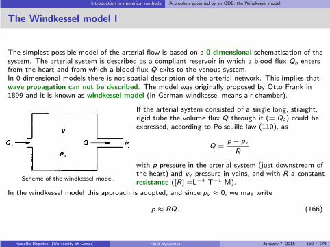
Introduction to numerical methods A problem governed by an ODE: the Windkessel model
The Windkessel model I
The simplest possible model of the arterial flow is based on a 0-dimensional schematisation of thesystem. The arterial system is described as a compliant reservoir in which a blood flux Qh entersfrom the heart and from which a blood flux Q exits to the venous system.In 0-dimensional models there is not spatial description of the arterial network. This implies thatwave propagation can not be described. The model was originally proposed by Otto Frank in1899 and it is known as windkessel model (in German windkessel means air chamber).
a
Scheme of the windkessel model.
If the arterial system consisted of a single long, straight,rigid tube the volume flux Q through it (= Qa) could beexpressed, according to Poiseuille law (110), as
Q =p − pv
R,
with p pressure in the arterial system (just downstream ofthe heart) and vv pressure in veins, and with R a constantresistance ([R] =L−4 T−1 M).
In the windkessel model this approach is adopted, and since pv ≈ 0, we may write
p ≈ RQ. (166)
Rodolfo Repetto (University of Genoa) Fluid dynamics January 7, 2015 160 / 179

Introduction to numerical methods A problem governed by an ODE: the Windkessel model
The Windkessel model II
The arterial system is considered compliant and its volume V is related to the arterial pressure bythe following relationship
p = V /C , (167)
where C is a constant compliance ([C ] = L4T 2M−1).In 0-dimensional models there is no equation of motion and only the conservation of mass isimposed. In this case the continuity equation can be written as
dV
dt= Qh − Q, (168)
where Qh denotes the flux ejected by the heart into the arterial system and Q is the flux from thearterial system to veins. Note that Q does not need be equal to Qh because of the compliance ofthe arterial system (which implies that V (t) depends on time). Substituting (166) and (167) into(168) we obtain
dV
dt= Qh − V
RC, (169)
or, equivalently,dp
dt=
Qh
C− p
RC, (170)
Rodolfo Repetto (University of Genoa) Fluid dynamics January 7, 2015 161 / 179

Introduction to numerical methods Simple integration schemes for ODEs
Solution of ordinary differential equations (ODE)
Let us consider a generic first order ordinary differential equation (ODE):
dy
dx= f (x , y), (171)
with boundary condition y(0) = y .The objective of the following slides is to show how to solve it using finite difference methods.
Rodolfo Repetto (University of Genoa) Fluid dynamics January 7, 2015 162 / 179
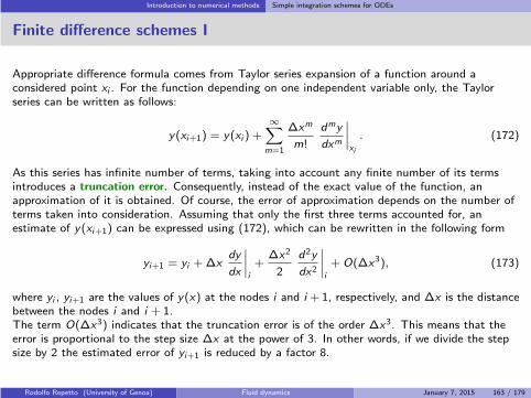
Introduction to numerical methods Simple integration schemes for ODEs
Finite difference schemes I
Appropriate difference formula comes from Taylor series expansion of a function around aconsidered point xi . For the function depending on one independent variable only, the Taylorseries can be written as follows:
y(xi+1) = y(xi ) +∞∑
m=1
∆xm
m!
dmy
dxm
∣∣∣∣xi
. (172)
As this series has infinite number of terms, taking into account any finite number of its termsintroduces a truncation error. Consequently, instead of the exact value of the function, anapproximation of it is obtained. Of course, the error of approximation depends on the number ofterms taken into consideration. Assuming that only the first three terms accounted for, anestimate of y(xi+1) can be expressed using (172), which can be rewritten in the following form
yi+1 = yi +∆xdy
dx
∣∣∣∣i
+∆x2
2
d2y
dx2
∣∣∣∣i
+ O(∆x3), (173)
where yi , yi+1 are the values of y(x) at the nodes i and i +1, respectively, and ∆x is the distancebetween the nodes i and i + 1.The term O(∆x3) indicates that the truncation error is of the order ∆x3. This means that theerror is proportional to the step size ∆x at the power of 3. In other words, if we divide the stepsize by 2 the estimated error of yi+1 is reduced by a factor 8.
Rodolfo Repetto (University of Genoa) Fluid dynamics January 7, 2015 163 / 179

Introduction to numerical methods Simple integration schemes for ODEs
Finite difference schemes II
Directly from (172) one can find an estimate of the first order derivative as
dy
dx
∣∣∣∣i
=yi+1 − yi
∆x− ∆x
2
d2y
dx2
∣∣∣∣i
+ O(∆x2), (174)
One can notice, that the following finite difference expression
dy
dx
∣∣∣∣i
≃ yi+1 − yi
∆x, (175)
approximates the derivative of y(x) at node i with first order accuracy, i.e. O(∆x). This formulais called the forward difference.A similar approach can be applied to derive the backward difference formula. To this end theTaylor series expansion is performed to provide an estimate of yi−1
yi−1 = yi −∆xdy
dx
∣∣∣∣i
+∆x2
2
d2y
dx2
∣∣∣∣i
+ O(∆x3), (176)
which gives the backward difference formula approximated to the first order as
dy
dx
∣∣∣∣i
≃ yi − yi−1
∆x. (177)
Rodolfo Repetto (University of Genoa) Fluid dynamics January 7, 2015 164 / 179
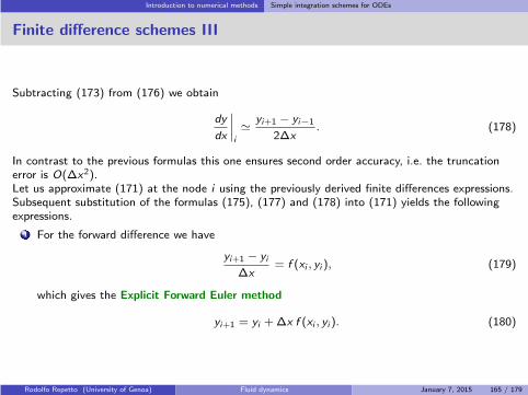
Introduction to numerical methods Simple integration schemes for ODEs
Finite difference schemes III
Subtracting (173) from (176) we obtain
dy
dx
∣∣∣∣i
≃ yi+1 − yi−1
2∆x. (178)
In contrast to the previous formulas this one ensures second order accuracy, i.e. the truncationerror is O(∆x2).Let us approximate (171) at the node i using the previously derived finite differences expressions.Subsequent substitution of the formulas (175), (177) and (178) into (171) yields the followingexpressions.
1 For the forward difference we have
yi+1 − yi
∆x= f (xi , yi ), (179)
which gives the Explicit Forward Euler method
yi+1 = yi +∆x f (xi , yi ). (180)
Rodolfo Repetto (University of Genoa) Fluid dynamics January 7, 2015 165 / 179
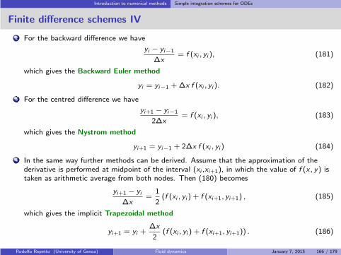
Introduction to numerical methods Simple integration schemes for ODEs
Finite difference schemes IV
2 For the backward difference we have
yi − yi−1
∆x= f (xi , yi ), (181)
which gives the Backward Euler method
yi = yi−1 +∆x f (xi , yi ). (182)
3 For the centred difference we have
yi+1 − yi−1
2∆x= f (xi , yi ), (183)
which gives the Nystrom method
yi+1 = yi−1 + 2∆x f (xi , yi ) (184)
4 In the same way further methods can be derived. Assume that the approximation of thederivative is performed at midpoint of the interval (xi ,xi+1), in which the value of f (x , y) istaken as arithmetic average from both nodes. Then (180) becomes
yi+1 − yi
∆x=
1
2(f (xi , yi ) + f (xi+1, yi+1) , (185)
which gives the implicit Trapezoidal method
yi+1 = yi +∆x
2(f (xi , yi ) + f (xi+1, yi+1)) . (186)
Rodolfo Repetto (University of Genoa) Fluid dynamics January 7, 2015 166 / 179

Introduction to numerical methods Simple integration schemes for ODEs
Bisection method I
The method is applicable for solving the equation f (x) = 0 for the real variable x , where f is acontinuous function defined on an interval [a, b] and f (a) and f (b) have opposite signs. In thiscase a and b are said to bracket a root since, by the intermediate value theorem, the continuousfunction f must have at least one root in the interval (a, b).
Bisection method: Step 1Given a function f (x), we have to choose the initial values a e b, within which only one root (i.e.f (x) = 0) lies. In this case we have that f (a) · f (b) < 0.
Rodolfo Repetto (University of Genoa) Fluid dynamics January 7, 2015 167 / 179
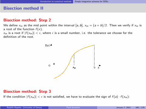
Introduction to numerical methods Simple integration schemes for ODEs
Bisection method II
Bisection method: Step 2We define xm as the mid point within the interval [a, b], xm = (a+ b)/2. Then we verify if xm isa root of the function f (x).xm is a root if |f (xm)| < ǫ, where ǫ is a small number, i.e. the tolerance we choose for thedefinition of the root.
Bisection method: Step 3If the condition |f (xm)| < ǫ is not satisfied, we have to evaluate the sign of f (a) · f (xm):
Rodolfo Repetto (University of Genoa) Fluid dynamics January 7, 2015 168 / 179
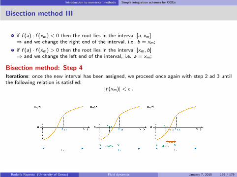
Introduction to numerical methods Simple integration schemes for ODEs
Bisection method III
if f (a) · f (xm) < 0 then the root lies in the interval [a, xm]⇒ and we change the right end of the interval, i.e. b = xm;
if f (a) · f (xm) > 0 then the root lies in the interval [xm, b]⇒ and we change the left end of the interval, i.e. a = xm;
Bisection method: Step 4Iterations: once the new interval has been assigned, we proceed once again with step 2 ad 3 untilthe following relation is satisfied:
|f (xm)| < ǫ .
Rodolfo Repetto (University of Genoa) Fluid dynamics January 7, 2015 169 / 179

Appendix A: material derivative of the Jacobian
Appendix A:
material derivative of the Jacobian
Rodolfo Repetto (University of Genoa) Fluid dynamics January 7, 2015 170 / 179

Appendix A: material derivative of the Jacobian Determinants
Determinants
Definition:A permutation i , j , . . . , p of the first n integers 1, 2, . . . n is called even or odd according as thenatural order can be restored by an even or odd number of interchanges.
Definition: The determinant of a n × n matrix A with elements aij is
detA =∑
±a1ia2j . . . anp , (187)
where the summation is taken over all permutations i , j , . . . , p of the integer numbers 1, 2, . . . , n,and the sign is positive for even permutations and negative for odd ones.
Therefore, for instance, the determinant of a 3× 3 matrix A is
detA =a11a22a33 + a12a23a31 + a13a21a32
− a12a21a33 − a11a23a32 − a13a22a31.
Note that in each term of the sum there is only one element from each row and each column.
Derivative of a determinantIf the elements of a n × n matrix A are function of a variable s, so that aij (s), the derivative withrespect to s of detA is the sum of n determinants obtained by replacing one row of A by thederivatives of its elements.
Rodolfo Repetto (University of Genoa) Fluid dynamics January 7, 2015 171 / 179
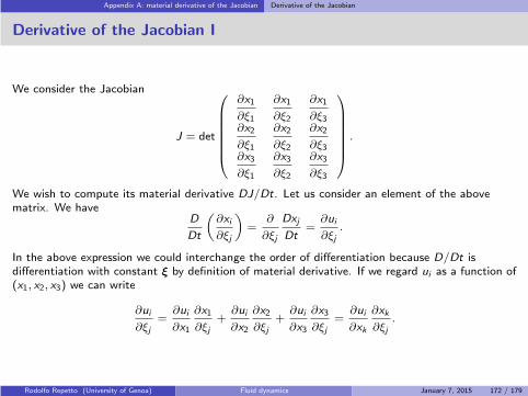
Appendix A: material derivative of the Jacobian Derivative of the Jacobian
Derivative of the Jacobian I
We consider the Jacobian
J = det
∂x1
∂ξ1
∂x1
∂ξ2
∂x1
∂ξ3∂x2
∂ξ1
∂x2
∂ξ2
∂x2
∂ξ3∂x3
∂ξ1
∂x3
∂ξ2
∂x3
∂ξ3
.
We wish to compute its material derivative DJ/Dt. Let us consider an element of the abovematrix. We have
D
Dt
(∂xi
∂ξj
)
=∂
∂ξj
Dxj
Dt=∂ui
∂ξj.
In the above expression we could interchange the order of differentiation because D/Dt isdifferentiation with constant ξ by definition of material derivative. If we regard ui as a function of(x1, x2, x3) we can write
∂ui
∂ξj=∂ui
∂x1
∂x1
∂ξj+∂ui
∂x2
∂x2
∂ξj+∂ui
∂x3
∂x3
∂ξj=∂ui
∂xk
∂xk
∂ξj.
Rodolfo Repetto (University of Genoa) Fluid dynamics January 7, 2015 172 / 179

Appendix A: material derivative of the Jacobian Derivative of the Jacobian
Derivative of the Jacobian II
We know that the derivative of a determinant of a 3× 3 matrix is the sum of three determinants,each of a matrix in which one row is differentiated. Thus to compute DJ/Dt we have to sum upthree terms the first of which is
det
∂u1
∂ξ1
∂u1
∂ξ2
∂u1
∂ξ3∂x2
∂ξ1
∂x2
∂ξ2
∂x2
∂ξ3∂x3
∂ξ1
∂x3
∂ξ2
∂x3
∂ξ3
= det
∂u1
∂xk
∂xk
∂ξ1
∂u1
∂xk
∂xk
∂ξ2
∂u1
∂xk
∂xk
∂ξ3∂x2
∂ξ1
∂x2
∂ξ2
∂x2
∂ξ3∂x3
∂ξ1
∂x3
∂ξ2
∂x3
∂ξ3
.
With k = 1 we have
det
∂u1
∂x1
∂x1
∂ξ1
∂u1
∂x1
∂x1
∂ξ2
∂u1
∂x1
∂x1
∂ξ3∂x2
∂ξ1
∂x2
∂ξ2
∂x2
∂ξ3∂x3
∂ξ1
∂x3
∂ξ2
∂x3
∂ξ3
=∂u1
∂x1J.
With k = 2, 3 we have ∂u1/∂xk times the determinant of a matrix with two identical rows, whichis therefore equal to zero.
Rodolfo Repetto (University of Genoa) Fluid dynamics January 7, 2015 173 / 179
Appendix A: material derivative of the Jacobian Derivative of the Jacobian
Derivative of the Jacobian III
Computing the other two term of the DJ/Dt we thus finally find
DJ
Dt=
(∂u1
∂x1+∂u2
∂x2+∂u3
∂x3
)
J = (∇ · u)J. (188)
Rodolfo Repetto (University of Genoa) Fluid dynamics January 7, 2015 174 / 179

Appendix B: the equations of motion in different coordinates systems
Appendix B:
the equations of motion in differentcoordinates systems
Rodolfo Repetto (University of Genoa) Fluid dynamics January 7, 2015 175 / 179

Appendix B: the equations of motion in different coordinates systems Cylindrical coordinates
Cylindrical coordinates
Let us consider cylindrical coordinates (z, r , ϕ), with corresponding velocity components(uz , ur , uϕ).
Continuity equation
∂uz
∂z+
1
r
∂
∂r(rur ) +
1
r
∂uϕ
∂ϕ= 0 (189)
Navier-Stokes equations
∂uz
∂t+ uz
∂uz
∂z+ ur
∂uz
∂r+
uϕ
r
∂uz
∂ϕ+
1
ρ
∂p
∂z− ν
[∂2uz
∂z2+
1
r
∂
∂r
(
r∂uz
∂r
)
+1
r2
∂2uz
∂ϕ2
]
= 0. (190)
∂ur
∂t+ uz
∂ur
∂z+ ur
∂ur
∂r+
uϕ
r
∂ur
∂ϕ−
u2ϕ
r+
1
ρ
∂p
∂r+
− ν
[∂2ur
∂z2+
1
r
∂
∂r
(
r∂ur
∂r
)
+1
r2
∂2ur
∂ϕ2− ur
r2− 2
r2
∂uϕ
∂ϕ
]
= 0. (191)
∂uϕ
∂t+ uz
∂uϕ
∂z+ ur
∂uϕ
∂r+
uϕ
r
∂uϕ
∂ϕ+
uruϕ
r+
1
ρr
∂p
∂ϕ+
− ν
[∂2uϕ
∂z2+
1
r
∂
∂r
(
r∂uϕ
∂r
)
+1
r2
∂2uϕ
∂ϕ2+
2
r2
∂ur
∂ϕ− uϕ
r2
]
= 0. (192)
Rodolfo Repetto (University of Genoa) Fluid dynamics January 7, 2015 176 / 179

Appendix B: the equations of motion in different coordinates systems Spherical polar coordinates
Spherical polar coordinates I
Let us consider spherical polar coordinates (r , ϑ, ϕ) (radial, zenithal and azimuthal), withcorresponding velocity components (ur , uϑ, uϕ).
Continuity equation
1
r2
∂
∂r
(r2ur
)+
1
r sinϑ
∂
∂ϑ(sinϑuϑ) +
1
r sinϑ
∂uϕ
∂ϕ= 0. (193)
Navier-Stokes equations
∂ur
∂t+ ur
∂ur
∂r+
uϑ
r
∂ur
∂ϑ+
uϕ
r sinϑ
∂ur
∂ϕ−
u2ϑ
r−
u2ϕ
r+
1
ρ
∂p
∂r+
− ν
[1
r2
∂
∂r
(
r2∂ur
∂r
)
+1
r2 sinϑ
∂
∂ϑ
(
sinϑ∂ur
∂ϑ
)
+1
r2 sin2 ϑ
∂2ur
∂ϕ2+
−2ur
r2− 2
r2 sinϑ
∂(uϑ sinϑ)
∂ϑ− 2
r2 sinϑ
∂uϕ)
∂ϕ
]
= 0. (194)
∂uϑ
∂t+ ur
∂uϑ
∂r+
uϑ
r
∂uϑ
∂ϑ+
uϕ
r sinϑ
∂uϑ
∂ϕ+
uruϑ
r−
u2ϕ cotϑ
r+
1
ρr
∂p
∂ϑ+
− ν
[1
r2
∂
∂r
(
r2∂uϑ
∂r
)
+1
r2 sinϑ
∂
∂ϑ
(
sinϑ∂uϑ
∂ϑ
)
+1
r2 sin2 ϑ
∂2uϑ
∂ϕ2+
Rodolfo Repetto (University of Genoa) Fluid dynamics January 7, 2015 177 / 179
Appendix B: the equations of motion in different coordinates systems Spherical polar coordinates
Spherical polar coordinates II
+2
r2
∂ur
∂ϑ− uϑ
r2 sin2 ϑ− 2 cosϑ
r2 sin2 ϑ
∂uϕ)
∂ϕ
]
= 0. (195)
∂uϕ
∂t+ ur
∂uϕ
∂r+
uϑ
r
∂uϕ
∂ϑ+
uϕ
r sinϑ
∂uϕ
∂ϕ+
uruϕ
r+
uϑuϕ cotϑ
r+
1
ρr sinϑ
∂p
∂ϕ+
− ν
[1
r2
∂
∂r
(
r2∂uϕ
∂r
)
+1
r2 sinϑ
∂
∂ϑ
(
sinϑ∂uϕ
∂ϑ
)
+1
r2 sin2 ϑ
∂2uϕ
∂ϕ2+
+2
r2 sinϑ
∂ur
∂ϕ+
2 cosϑ
r2 sin2 ϑ
∂uϑ
∂ϕ− uϕ
r2 sin2 ϑ
]
= 0. (196)
Rodolfo Repetto (University of Genoa) Fluid dynamics January 7, 2015 178 / 179
References
References
D. J. Acheson. Elementary Fluid Dynamics. Oxford University Press, 1990.
R. Aris. Vectors, tensors, and the basic equations of fluid mechanics. Dover Publications INC.,New York, 1962.
G. I. Barenblatt. Scaling. Cambridge University Press, 2003.
G. K. Batchelor. An Introduction to Fluid Dynamics. Cambridge University Press, 1967.
J. H. Ferziger and M. Peric. Computational methods for fluid dynamics, volume 3. SpringerBerlin, 2002.
H. Ockendon and J. R. Ockendon. Viscous Flow. Cambridge University Press, 1995. ISBN0521458811.
R. H. Pletcher, J. C. Tannehill, and D. Anderson. Computational fluid mechanics and heat
transfer. CRC Press, 2012.
C. Pozrikidis. Fluid Dynamics: Theory, Computation, and Numerical Simulation. Springer,softcover reprint of hardcover 2nd ed. 2009 edition, Nov. 2010. ISBN 1441947191.
E. F. Toro. Riemann Solvers and Numerical Methods for Fluid Dynamics, Third Edition.Springer–Verlag, 2009.
H. K. Versteeg and W. Malalasekera. An introduction to computational fluid dynamics: the finite
volume method. Pearson Education, 2007.
Rodolfo Repetto (University of Genoa) Fluid dynamics January 7, 2015 179 / 179