notes on mathematics of quantum mechanics - physsturgut/p455/qm-math4.pdf · 1 hilbert spaces...
TRANSCRIPT
Notes on Mathematics of Quantum Mechanics
Sadi Turgut
Contents
1 Hilbert Spaces 21.1 Definition of Hilbert Spaces . . . . . . . . . . . . . . . . . . . . . . . . . . 41.2 Basic Linearity Notions . . . . . . . . . . . . . . . . . . . . . . . . . . . . . 121.3 Basic Notions in Hilbert Spaces . . . . . . . . . . . . . . . . . . . . . . . . 14
2 Operators 192.1 Hermitian Conjugation . . . . . . . . . . . . . . . . . . . . . . . . . . . . . 222.2 Dirac Notation . . . . . . . . . . . . . . . . . . . . . . . . . . . . . . . . . 25
2.2.1 Matrix Example . . . . . . . . . . . . . . . . . . . . . . . . . . . . . 262.2.2 Expansion of Identity . . . . . . . . . . . . . . . . . . . . . . . . . . 27
2.3 Matrix Representation . . . . . . . . . . . . . . . . . . . . . . . . . . . . . 282.4 Trace . . . . . . . . . . . . . . . . . . . . . . . . . . . . . . . . . . . . . . . 30
3 Spectral Theory 333.1 Eigenvalue Equation . . . . . . . . . . . . . . . . . . . . . . . . . . . . . . 333.2 Diagonalization . . . . . . . . . . . . . . . . . . . . . . . . . . . . . . . . . 353.3 Projections . . . . . . . . . . . . . . . . . . . . . . . . . . . . . . . . . . . 37
4 Functions of Operators 414.1 Functions of Normal Operators . . . . . . . . . . . . . . . . . . . . . . . . 414.2 Alternative definition of functions of operators . . . . . . . . . . . . . . . . 45
5 Positive Operators 475.1 Positive Definiteness for Matrices . . . . . . . . . . . . . . . . . . . . . . . 485.2 Lowner Partial Order . . . . . . . . . . . . . . . . . . . . . . . . . . . . . . 505.3 Polar decomposition . . . . . . . . . . . . . . . . . . . . . . . . . . . . . . 51
6 Tensor Product 526.1 Kronecker Products . . . . . . . . . . . . . . . . . . . . . . . . . . . . . . . 526.2 Tensor Product of Hilbert Spaces . . . . . . . . . . . . . . . . . . . . . . . 53
1

1 Hilbert Spaces
Hilbert space is the basic mathematical structure used in the description of the physics ofquantum systems. For this reason, it is necessary to master its mathematics. Why do weneed Hilbert spaces? Because, the states of any physical system are somehow representedas vectors in some Hilbert space. We can understand the physics of the system by doingsome mathematical calculations in and about this space. Quantum mechanics is usuallyconsidered difficult because there is no direct connection between the physics and thecorresponding mathematics. However, once this connection is accepted, there is nothingcomplicated about the mathematics of quantum mechanics.
An analogy to the classical mechanicsmay perhaps clarify this connection. Con-sider, for example, the classical mechanicsof an object attached to the end of a fixedspring. By the state of the object at agiven time we mean a complete descriptionof what the object is doing at that moment.We can give this description by specifyingthe position x and the velocity x at the givenmoment. Therefore, we can represent the state mathematically as position-velocity values(x, x).
Classical Mechanics: state←→ (x, x) .
Sometimes we gloss over the distinction between the physical state and call directly thepair of numbers (x, x) as the state. The set that contains all states is called the statespace. Here, the state space is the whole 2D plane, which can equivalently be named R2.Basically, every point of this space is in one-to-one correspondence with the physical states.
The pair of numbers (x, x) somehow contain all information about the object that wecan know. We can compute any property of the particle as a function of these two numbers.For example, the energy is E = E(x, x) = (mx2 + kx2)/2, the instantaneous accelerationat this moment is a = a(x, x) = −kx/m, etc. In all cases, we assume that we know thedynamics of the system. That means that, if we know the initial state at time t = 0, thenwe can in principle compute the state at any time. For example, if (x, x) is the state ofthe object at time t = 0, the state (xt, xt) at time t is also a function of (x, x). For theobject attached to the spring, these are
xt = f(x, x; t) = x cosωt+x
ωsinωt ,
xt = g(x, x; t) = −ωx sinωt+ x cosωt .
2

In short, any physically relevant property ofthe system is computed in terms of the state(x, x) at any time. The mathematical rep-resentation of the states may not be unique.For example, in the case of Hamiltonianapproach to classical dynamics, we chooseposition-momentum pair (x, p) as the math-ematical structure to represent the state.
For the quantum mechanical descriptionof the same system, we need much more than a pair of real numbers for describing thestate. For example, we use a wavefunction, say ψ(x), for representing the state of theobject. Somehow, this function contains all information about the physical state of theobject.
Quantum Mechanics: state←→ ψ(x) .
The wavefunction ψ is a mathematical construct for representing the physical state. Asabove, we can consider ψ as a member of a state space that contains all possible states. Inthis case, the state space is essentially the set of complex-valued square-integrable functionsof one variable. The main difference from the classical case is that now, by knowing ψ,we may not form an immediate picture of what the object is really doing at the givenmoment. Of course, our classical minds can never appreciate a quantum state, so we needto somehow accept this state of affairs when doing quantum mechanics.
The precise mathematical object that needs to be used for representing states dependson the physical system we are interested in. A simple wavefunction may be sufficient forone or a few fixed particles, but we need different mathematical objects for some othersystems. For example, a “Fock space” construction is necessary if particle creation andannihilation processes are possible and a simple column matrix might be sufficient fordescribing the spin states of particles or some other few-level systems. Although differentsystems need different mathematical structures for representing the states, all of them havesome common features. It appears that we can explain quantum mechanics by using onlythose common features. For example, in all cases the state space turns out to be a complexHilbert space. The states are represented by unit vectors in that space. The mathematicaloperations needed to compute averages, probabilities etc. are all similar. This is the reasonwhy we tend to provide an abstract description of the mathematics of quantum mechanics.We give the rules for abstract Hilbert spaces, so that the same rules can be applied in allspecific cases we may investigate.
Let’s return back to where we have started from. For any physical system, there will bea Hilbert space H such that any physically possible state of the system is mathematicallyrepresented by a (unit) vector |ψ〉 in H.
Quantum Mechanics: state←→ |ψ〉 ∈ H .
Usually we forget about the distinction between the “physical states” and their mathe-
3

matical representations and call |ψ〉 directly as “the state”. As above, the state somehowcontains all information about the system. This information is not “plainly visible”; weneed to use proper mathematical tools for extracting this information. For example, if aphysical quantity is measured, we can compute the possible outcomes, their probabilitiesand the average values as a function of the state. Also, if the state is given at a given timet0, we can compute the state at any other time t. Any experimentally measurable propertyof the system can somehow be computed by using only the state |ψ〉.
To repeat, from the point of view of the mathematical representation of states of asystem, there is not much difference between the classical and quantum mechanics. Theonly problem of quantum mechanics is that translating the mathematical information tophysical picture is a little bit complicated.
1.1 Definition of Hilbert Spaces
As a result, we need learn something about the Hilbert spaces for the purpose of learningquantum mechanics. We will start with the definition of Hilbert spaces. Hilbert spaces areessentially vector spaces with an inner product defined on it. Most of the time, the vectorswill be shown in the ket notation, like |ψ〉. This appears to be a very useful notation inquantum mechanics, especially it simplifies the Dirac bra-ket notation, which we will seelater. Here, the ket notation also implies that we are working with an abstract Hilbertspace. If specific Hilbert spaces are used, we tend to drop the ket symbol. For example, ψis used for column matrices, ψ(x) for wavefunctions, etc.
The formal definition of a Hilbert space is as follows: A set H is called a Hilbert spaceif the following three conditions are satisfied:
(I) H is a vector space.
The elements of H are vectors shown by |ψ〉 etc. The “vector addition” and“multiplication with a scalar” are the operations defined on H. Given vectors|ψ1〉 , . . . , |ψn〉 and scalar numbers c1, . . . , cn, the linear combination
c1 |ψ1〉+ · · ·+ cn |ψn〉
is also a vector. The linear combination is also called superposition by physicists.The zero vector is shown by a 0 without a ket sign.
If the scalar numbers used, ci, can be complex, then H is called a complex Hilbertspace. If scalars have to be real, then H is called a real Hilbert space. Quantummechanics is always done on complex Hilbert spaces.
4
• (II) There is an inner product 〈·|·〉 defined on the vectors.
Inner product is an operation between two vectors which produces a scalar num-ber. In other words, if |ψ〉 and |φ〉 are two vectors in H, then 〈ψ|φ〉 is a scalarnumber. Its defining properties are
(1) 〈ψ|φ〉∗ = 〈φ|ψ〉.(2) 〈ψ|φ〉 is linear in |φ〉,
if |φ〉 = c1 |φ1〉+ c2 |φ2〉 then 〈ψ|φ〉 = c1〈ψ|φ1〉+ c2〈ψ|φ2〉 .
and anti-linear in ψ,
if |ψ〉 = d1 |ψ1〉+ d2 |ψ2〉 then 〈ψ|φ〉 = d∗1〈ψ1|φ〉+ d∗2〈ψ2|φ〉 .
(3) 〈ψ|ψ〉 ≥ 0. Moreover, 〈ψ|ψ〉 = 0 if and only if ψ = 0.
Note that 〈ψ|ψ〉 is a real number by (1). Property (3) states that this numberis non-negative. Moreover, if the vector is nonzero (|ψ〉 6= 0) then 〈ψ|ψ〉 is apositive number. Inner product enables us to define the lengths of vectors as
‖ψ‖ =√〈ψ|ψ〉 .
This quantity is called the norm (or length) of the vector ψ. Note that by (3),non-zero vectors have non-zero lengths and only the zero vector has length zero.The “unit vectors” have norm 1 and are called normalized. For any vector ψ,the vector
|ψ′〉 =1
‖ψ‖|ψ〉
is a normalized vector. This process is sometimes called normalization.
• (III) H is complete.
Completeness is a topological property that is necessary only for infinite di-mensional Hilbert spaces. In most of the physics oriented applications of Hilbertspaces, completeness property is never used. However, a short description will beprovided in here for general information. Note that the inner product enables us
5

to define norms ‖·‖ of vectors, which enables us to measure the distance betweentwo vectors |ψ〉 and |φ〉 as the norm of their difference ‖|ψ〉 − |φ〉‖ = ‖ψ − φ‖.Using this distance, we can define convergence of sequences of vectors. Let|ψ1〉, |ψ2〉, . . . be an infinite sequence of vectors. We say that the sequence |ψn〉converges to the vector |φ〉 if the distance between |ψn〉 and |φ〉 goes to 0.
limn→∞
|ψn〉 = |φ〉 if limn→∞
‖|ψn〉 − |φ〉‖ = 0 .
A Cauchy sequence is a sequence which the vectors of the sequence approach toeach other as the index tends to infinity. In other words,
|ψ1〉 , |ψ2〉 , . . . is Cauchy if limn,m→∞
‖|ψn〉 − |ψm〉‖ = 0 .
The vector space H is called complete if every Cauchy sequence converges tosome vector.
The above definition is the formal definition of the completeness property. Es-sentially it says that sequences which appear to converge do converge to somevector. We usually use this property in series expansions of vectors in a givenbasis, like
|φ〉 =∞∑n=1
cn |φn〉
where “superpositions of infinitely many vectors” are involved. As there areinfinitely many terms in the series, we need to take a limit to evaluate the sum.The existence of the limit is then an important question. Completeness propertyenables us to decide on the existence of the series sum |φ〉 by investigating theterms in the series.
There are several examples of Hilbert spaces. Some of these spaces find applicationsin some various areas of physics, engineering and mathematics. Just a few examples aregiven below.
6

EXAMPLE
The three-dimensional vectors with the “dot product” forms a real Hilbert space.For two vectors ~A and ~B in this space, we define the inner product as
~A · ~B = |A| |B| cos θ
where θ is the angle between the vectors. Alternatively, we can define the innerproduct in terms of the components of the vectors.
~A = Axı + Ay + Azk ,
~B = Bxı +By +Bzk ,
−→ ~A · ~B = AxBx + AyBy + AzBz .
The space is sometimes shown by R3. You can check that R3 satisfies all propertiesof being a Hilbert space.
Since this space (or similar real spaces with different dimensions Rn) is veryfamiliar to us, we can use it as some sort of a pictorial guide in understanding thegeometry of complex Hilbert spaces.
EXAMPLE
The n × 1 column vectors also forms a Hilbert space. The vectors are representedby n scalar numbers written in an array. The vector operations are obvious.
α =
a1a2...an
, β =
b1b2...bn
, −→ cα + dβ =
ca1 + db1ca2 + db2
...can + dbn
.
The zero vector is a column vector with zero entries
0 =
00...0
.
Although we represent two different mathematical objects with the same symbol
7

(namely, the zero vector and the scalar number zero are both shown by 0) thisrarely causes confusion.
Finally, the inner product of two vectors are defined as 〈α|β〉 = α†β,
〈α|β〉 = α†β =[a∗1 a∗2 . . . a∗n
]b1b2...bn
= a∗1b1 + a∗2b2 + · · ·+ a∗nbn .
It can easily be checked that these vectors also form a Hilbert space. Since thesevectors are essentially a list of n independent numbers, the associated Hilbert spaceis usually called Rn if real numbers are used and Cn if complex numbers are used.
It is important to note that the previous example of real vectors in 3D can alsobe considered as a Hilbert space of column vectors.
~A = Axı + Ay + Azk −→ A =
AxAyAz
.
The two Hilbert spaces agree; only the way the vectors are presented are different.Sometimes people may change notation whenever they feel convenient. For thisreason, we will show both vectors spaces by the R3 notation.
Just like the definition for column matrices, it is possible to define Hilbert spaceson row vectors or even rectangular matrices with a fixed size. However, in quantummechanics, it is notationally more convenient to represent the states as columnvectors. For this reason, the definition above is sufficient for us. This Hilbert spaceis used for the representation of states of any n-level system.
EXAMPLE
The set of square-integrable functions can also be made a Hilbert space. Considerfor example a 1D space. Take a complex-valued function of a single real variable x.
f : R→ C .
We say that f is square-integrable if the integral of the modulus square of f is
8

convergent. In notation
f is square integrable if
∫ +∞
−∞|f(x)|2 dx <∞ .
It can be shown that if f and g are square-integrable functions, then their linearcombinations h(x) = c1f(x) + c2g(x) are also square-integrable. This makes the setof square integrable functions a vector space. If you are accustomed to the pictureof vectors as “pointed arrows”, the vector space of square-integrable functions willappear very strange to you because you will have difficulty of picturing a functionf(x) as a pointed arrow. It is difficult, but not impossible.
Now, the inner product is defined in the standard way
〈f |g〉 =
∫ +∞
−∞f(x)∗g(x)dx .
The square-integrability condition ensures that the inner product integrals are alwaysconvergent.
There is a small detail that you may want to know. Square-integrable functionscan in principle have any number and type of discontinuities. Consider for exampletwo square integrable functions f and g which differ only at a few points (i.e.,f(x) − g(x) = 0 except a few x values). Compared to all other values that theyagree, the difference between f and g is not important. In fact, when we try tocompute the distance between the two functions by using the inner product above,we get
‖f − g‖2 =
∫ +∞
−∞|f(x)− g(x)|2 dx = 0 .
Since only the zero vector should have norm 0, we should really think these twofunctions f and g to be the “same”. In other words, physically irrelevant differencesbetween functions should be thrown away. Mathematicians can do this systemati-cally and the set that you will get is called L2(R). But, we can think of it basicallyas “square-integrable functions”.
This Hilbert space appears as the state space of a spinless particle living inone-dimension. It can readily be generalized to a N spinless particles living in d-dimensional space. In that case, the functions f are complex-valued functions of dNreal parameters: f : RdN −→ C.
9

EXAMPLE
The square-integrable function example can be generalized easily. We may consideran interval [a, b] of the real line, (which might be the whole line itself). Let w(x)be a function which is positive everywhere on that interval. This is usually called aweight function. Consider functions defined on this interval. We can define an innerproduct between two such functions as
〈f |g〉 =
∫ b
a
f(x)∗w(x)g(x)dx .
Now, a Hilbert space can easily be defined based on this definition. Obviously, onlythe vectors that has a finite length (‖f‖ <∞) are elements of the Hilbert space.
This kind of Hilbert spaces appear frequently in various applications. Especiallythe orthogonal polynomials (which form a significant part of the special functions)are better treated with the above Hilbert space approach.
Let us see what can be done with an inner product on an abstract Hilbert space. Thefirst thing we do is to define a norm which can be used to measure the distance betweenvectors. This is a place where the ket notation can be cumbersome. So instead of ‖|ψ〉‖,we will use ‖ψ‖.
The essential relation that shows that the norm is a distance is the triangle inequality :
‖α− γ‖ ≤ ‖α− β‖+ ‖β − γ‖ ,
which essentially says that the sidelength of a triangle is smaller than the sum of the othertwo sidelengths. The same inequality can be compactly expressed as ‖ψ + φ‖ ≤ ‖ψ‖+‖φ‖.Another inequality is the parallelogram law
‖ψ + φ‖2 + ‖ψ − φ‖2 = 2 ‖ψ‖2 + 2 ‖φ‖2
which relates the sums of squares of the diagonals of a parallelogram to that of the sides.This inequality is peculiar only to the inner-product spaces where the distance is definedby using the inner product.
10
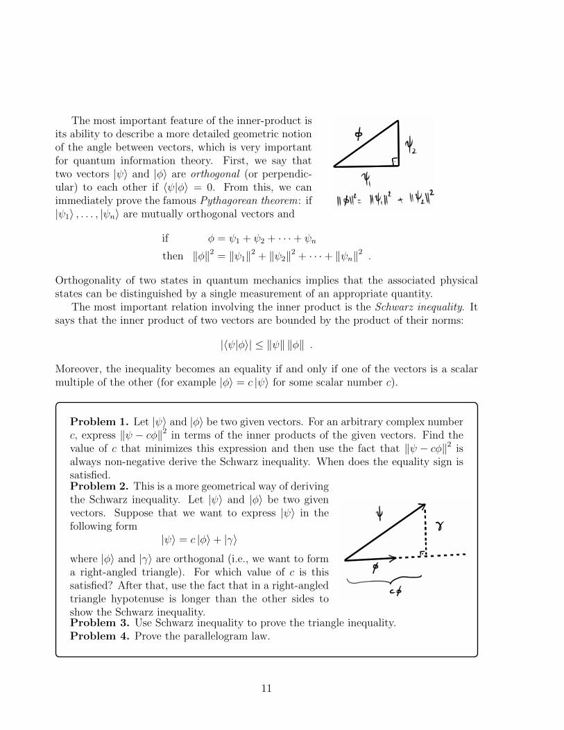
The most important feature of the inner-product isits ability to describe a more detailed geometric notionof the angle between vectors, which is very importantfor quantum information theory. First, we say thattwo vectors |ψ〉 and |φ〉 are orthogonal (or perpendic-ular) to each other if 〈ψ|φ〉 = 0. From this, we canimmediately prove the famous Pythagorean theorem: if|ψ1〉 , . . . , |ψn〉 are mutually orthogonal vectors and
if φ = ψ1 + ψ2 + · · ·+ ψn
then ‖φ‖2 = ‖ψ1‖2 + ‖ψ2‖2 + · · ·+ ‖ψn‖2 .
Orthogonality of two states in quantum mechanics implies that the associated physicalstates can be distinguished by a single measurement of an appropriate quantity.
The most important relation involving the inner product is the Schwarz inequality. Itsays that the inner product of two vectors are bounded by the product of their norms:
|〈ψ|φ〉| ≤ ‖ψ‖ ‖φ‖ .
Moreover, the inequality becomes an equality if and only if one of the vectors is a scalarmultiple of the other (for example |φ〉 = c |ψ〉 for some scalar number c).
Problem 1. Let |ψ〉 and |φ〉 be two given vectors. For an arbitrary complex numberc, express ‖ψ − cφ‖2 in terms of the inner products of the given vectors. Find thevalue of c that minimizes this expression and then use the fact that ‖ψ − cφ‖2 isalways non-negative derive the Schwarz inequality. When does the equality sign issatisfied.Problem 2. This is a more geometrical way of derivingthe Schwarz inequality. Let |ψ〉 and |φ〉 be two givenvectors. Suppose that we want to express |ψ〉 in thefollowing form
|ψ〉 = c |φ〉+ |γ〉
where |φ〉 and |γ〉 are orthogonal (i.e., we want to forma right-angled triangle). For which value of c is thissatisfied? After that, use the fact that in a right-angledtriangle hypotenuse is longer than the other sides toshow the Schwarz inequality.Problem 3. Use Schwarz inequality to prove the triangle inequality.Problem 4. Prove the parallelogram law.
11

If the Hilbert space is a real vector space, then the angle between nonzero vectors ψand φ is simply defined as
cos θ =〈ψ|φ〉‖ψ‖ ‖φ‖
,
where 0 ≤ θ ≤ π (from Schwarz inequality we can see that −1 ≤ cos θ ≤ 1). In quantummechanics, however, we have to use complex numbers and in this case the expression abovedoes not make sense. But, it might be useful to define an angle between vectors with thefollowing,
cos θ =|〈ψ|φ〉|‖ψ‖ ‖φ‖
.
Here, 0 ≤ cos θ ≤ 1 and therefore 0 ≤ θ ≤ π/2.There are two special cases that should be noted. The case θ = 0, where we interpret
that ψ and φ are “parallel” to each other, which corresponds to the equality case inSchwarz inequality. This is the case where each vector is a scalar multiple of the other,like |φ〉 = c |ψ〉. We do not have well-defined notions of anti-parallelism, we can say that|ψ〉, − |ψ〉, i |ψ〉 etc. are all parallel to |ψ〉. If |φ〉 = c |ψ〉 and c = |c| eiα, then we just saythat the phase difference between these vectors is α.
The special case in the other extreme is θ = π/2, in which case we have said that |φ〉and |ψ〉 are orthogonal to each other. For all the other cases, it is possible to think of thesevectors making the specified angle with each other.
1.2 Basic Linearity Notions
Linear Independence: Let |ψ1〉 , . . . , |ψn〉 be vectors in H. By using the basic operationsof a vector space, i.e., multiplication with a scalar and vector addition, we can form thefollowing general expression
c1 |ψ1〉+ c2 |ψ2〉+ · · ·+ cn |ψn〉 =n∑k=1
ck |ψk〉 ,
where ck are scalars. Such an expression is called a linear combination or a superpositionof vectors |ψ1〉 , |ψ2〉 , . . . , |ψn〉. The set of vectors {ψ1, . . . , ψn} is called linearly dependentif there are numbers c1, . . . , cn such that some of them are non-zero and
c1ψ1 + c2ψ2 + · · ·+ cnψn = 0 .
If this is the case, then it means that we can express one of the vectors in this set as asuperposition of others.
12
EXAMPLE
The set { ~A, ~B, ~C}, where ~A = i, ~B = j and ~C = 3i + 2j, is linearly dependent. In
that case we have 3 ~A + 2 ~B − ~C = 0. Therefore, we can express any vector in thisset as a superposition of others: ~A = (~C − 2 ~B)/3 or ~B = (~C − 3 ~A)/2 etc.
EXAMPLE
The set of functions {sinx, cosx, eix} are also linearly dependent since i sinx+cos x−eix = 0. Since all scalar coefficients are nonzero, we can express any of these functionsas a superposition of the other two.
The set of vectors {|ψ1〉 , . . . , |ψn〉} is called linearly independent if the equation
c1 |ψ1〉+ c2 |ψ2〉+ · · ·+ cn |ψn〉 = 0 ,
has only the trivial solution c1 = c2 = · · · = cn = 0. In this case, no vector in this set canbe expressed as a superposition of others. Moreover, if a vector |φ〉 is a superposition ofthese linearly independent vectors, i.e.,
|φ〉 = d1 |ψ1〉+ d2 |ψ2〉+ · · ·+ dn |ψn〉 ,
for some numbers dk, then these numbers are unique.Bases: The set of vectors {|ψ1〉 , . . . , |ψd〉} is called a basis (plural: bases) for the vector
space H if
(1) {|ψ1〉 , . . . , |ψd〉} is linearly independent and
(2) Any vector |φ〉 in H can be expressed as a superposition of these, i.e., there are scalarsc1, c2, . . . , cd such that
|φ〉 = c1 |ψ1〉+ c2 |ψ2〉+ · · ·+ cd |ψd〉 .
Because of linear independence, the numbers ck are unique. As a result, there is a one-to-one correspondence between the vectors φ in H and the d-tuplet of complex numbers(c1, c2, . . . , cd) in Cn (which are usually represented as d× 1 column vectors). The numberof vectors d in a basis is called the dimension of the vector spaceH and we write d = dimH.It can be shown that
13
• Any possible basis of H contains the same number of vectors in it, i.e., dimension is aproperty of the vector space which is independent of which particular basis is chosen.
• Any set of d = dimH linearly independent vectors is a basis.
• Any set of d+ 1 or more vectors are necessarily linearly dependent.
• If the set of n vectors, {α1, . . . , αn} is linearly independent, then n ≤ d. If n is strictlyless than d, then this set can be completed to a basis by appropriately choosing d− nother vectors. In other words, you can find αn+1, . . . , αd such that the set of d vectors{α1, . . . , αn, αn+1, . . . , αd} is a basis.
If it is not possible to construct a basis from a finite number of vectors, then we saythat the space is infinite dimensional and write dimH =∞.
Subspaces: A subset V of a Hilbert space H is called a subspace if that set isclosed under vector addition and multiplication with a scalar. In other words, for any|ψ1〉 , . . . , |ψn〉 ∈ V and any scalars ck, the linear combination
∑k ck |ψk〉 is in V . For ex-
ample, xy-plane in R3 is a subspace. Note that the zero vector 0 is always a member of asubspace.
There are two trivial subspaces of any vector space H. First one is the subset thatcontains a zero vector, i.e., V = {0}, and the other is H itself. All other subspaces arecalled proper subspaces.
For any set of vectors {|ψ1〉 , |ψ2〉 , . . . , |ψn〉}, all vectors that can be expressed as a super-position of these vectors, V = {|φ〉 : |φ〉 =
∑k ck |ψk〉} is a subspace. We say that V is the
subspace spanned by {|ψ1〉 , |ψ2〉 , . . . , |ψn〉}. Equivalently, we say that {|ψ1〉 , |ψ2〉 , . . . , |ψn〉}spans the subspace V . If the set {|ψ1〉 , |ψ2〉 , . . . , |ψn〉} is linearly independent then we saythat this set is a basis for the subspace it spans, and consequently we have n = dimV .
If V and W are two subspaces, then their intersection, V ∩ W , is a subspace. Forexample, in R3, the intersection of xy-plane with xz plane is the 1-dimensional x-axis.Their union is not necessarily a subspace. By V +W we denote the subspace spanned byall of the vectors in these subspaces. For example, in R3, if V is the x-axis (spanned by i)and W is the y-axis (spanned by j), then V +W is the xy-plane (spanned by {i, j}). Toexpress it in another way, V +W is the smallest subspace containing both V and W . Wehave the following identity for the dimensions
dim(V +W) + dim(V ∩W) = dimV + dimW .
1.3 Basic Notions in Hilbert Spaces
A set of vectors {|ψ1〉 , |ψ2〉 , . . . , |ψn〉} is called an orthonormal set if
(1) each vector is normalized, ‖ψ1‖ = · · · = ‖ψn‖ = 1, and
(2) different vectors are orthogonal (if i 6= j then 〈ψi|ψj〉 = 0).
14

We express these two conditions in short by 〈ψi|ψj〉 = δij. An orthonormal set is necessarilylinearly independent. To show this, suppose that
c1ψ1 + · · ·+ cnψn = 0 .
Take the inner product of this expression with ψk. As the inner product of ψk with zerovector is 0, we have
c1〈ψk|ψ1〉+ · · ·+ ck〈ψk|ψk〉 + · · ·+ cn〈ψk|ψn〉 = 0
c10 + · · ·+ ck1 + · · ·+ cn0 = 0
which leads to ck = 0. In other words, we necessarily have the trivial solution c1 = c2 =· · · = cn = 0 and therefore the set is linearly independent.
Orthonormal bases: We say that the set of vectors {|ψ1〉 , |ψ2〉 , . . . , |ψd〉} is an or-thonormal basis for H if it is an orthonormal set and a basis. Note that any orthonormalset with d = dimH vectors is necessarily an orthonormal basis.
There are various reasons why we are interested in orthonormal bases. One of the rea-sons is that the mathematical computations in such a basis is usually very simple. For ex-ample, consider the expansion of a vector |φ〉 in the orthonormal basis {|ψ1〉 , |ψ2〉 , . . . , |ψd〉}.
|φ〉 =∑k
ck |ψk〉 = c1 |ψ1〉+ · · ·+ cd |ψd〉 .
The expansion coefficients ck (the components) can be computed simply by taking an innerproduct with the corresponding basis vectors, i.e.,
ck = 〈ψk|φ〉 .
There is more. The norm and inner product can be computed in a very simple way fromthe expansion coefficients. For the norm,
‖φ‖2 =∑k
|ck|2 ,
which is nothing other than the Pythagorean theorem, and for |χ〉 =∑dk |ψk〉, the inner
product is
〈φ|χ〉 =∑k
c∗kdk .
We not only have a one-to-one correspondence between the vectors in H and the columnvectors in Cd, but also the inner product can be computed in either space. For |φ〉 =∑
k ck |ψk〉 the corresponding column vector is defined as
uφ =
c1c2...cd
,
15

i.e., the list of expansion coefficients in the orthonormal basis. This vector is called thematrix representation of |φ〉 in the chosen basis. Due to the fact that we have used anorthonormal basis, the inner products of the vectors in H and the corresponding vectorsin Cd are equal, i.e., 〈φ|χ〉 = u†φuχ. We will say more about matrix representations later.
EXAMPLE
Consider the following three vectors in R3
a1 =1√3
(i + j + k
),
a2 =1√2
(i− j
),
a3 =1√6
(i + j − 2k
).
The set {a1, a2, a3} is an orthonormal set. Since there are 3 vectors, this set is then
a basis for R3. Any given vector, such as ~B = 3i + 4j can be expressed in thisbasis as ~B = c1a1 + c2a2 + c3a3. In order to find the expansion coefficients, we justevaluate three inner products, i.e.,
c1 = a1 · ~B =7√3
,
c2 = a2 · ~B = − 1√2
,
c3 = a3 · ~B =7√6
,
As a result we have~B =
7√3a1 −
1√2a2 +
7√6a3 .
Any other method for finding these coefficients (such as solving linear equations)is usually longer than the simple method given above. Check that you can findthe length of the vector in either basis, i.e., you get the same value for ~B · ~B =B2x +B2
y +B2z = c21 + c22 + c23.
For n × 1 column matrices, the standard orthonormal basis is the set of vectors{e1, e2, . . . , en} where ek is the column vector whose kth row is 1 and all other elements
16

are 0, i.e.,
e1 =
100...0
, e2 =
010...0
, · · · , en =
000...1
.
Orthonormal bases in infinite dimensions: If dimH = ∞, we can find infinitelymany orthonormal vectors |ψk〉. Such an orthonormal set is a basis if any vector |φ〉 canbe expressed as the limit of a series
|φ〉 =∞∑k=1
ck |ψk〉 .
Since a limit is involved, the question of whether such series converge or not becomesimportant. This is where the completeness property of the Hilbert spaces enters into thepicture. We can summarize the situation as follows: If
∑k |ck|
2 is a convergent series, thenthe series expansion above converges to a vector |φ〉 in the Hilbert space. Note that theseries
∑k |ck|
2 is equal to the norm ‖φ‖2.The expansion coefficients are also computed in the same way: ck = 〈ψk|φ〉 and we
have the usual expression for the inner products of two vectors as well. These vectors canalso be represented by their expansion coefficients {ck}, but the column vectors formedwould be ∞× 1 in size.
Separability: Any complete inner product space is called a Hilbert space. But, inquantum mechanics, when we represent the states of a system as vectors in a Hilbertspace, we require one more property called separability. This is also a topologicalproperty but it can be expressed in a simple way in terms of orthonormal bases.We say that a given Hilbert space is separable if it has a countable orthonormalbasis. In other words, we must be able to find an orthonormal basis such that wecan label these vectors by natural numbers 0, 1, 2, . . . in a one-to-one correspondence.The separability issue arises in systems containing infinitely many particles, in whichcase we have to choose an appropriate subspace to describe the physics of the system.We will not be concerned with this issue in this course.
Change of basis: Sometimes we need to express a given vector |φ〉 in a differentorthonormal basis. Let us state a few properties of changing a basis. Suppose that{|ψ1〉 , . . . , |ψd〉} be an orthonormal basis for H. Let {|α1〉 , . . . , |αd〉} be another orthonor-mal basis. Any vector can be expanded in either basis. If a vector has a known expansion
17
in one basis, the expansion coefficients on the other basis can be obtained in the otherbasis as follows.
First, expand each αk in the former basis as
|αk〉 =d∑`=1
U`k |ψ`〉 . (1)
Here U`k are the expansion coefficients of the vector αk. These coefficients can be consideredas the elements of a d× d matrix U (the basis change matrix). Since both of the bases areorthonormal, we have
U`k = 〈ψ`|αk〉 .
Now, observe that U∗`k = 〈αk|ψ`〉 by the properties of the inner product. Therefore, thevectors of the former basis can be expanded in the second basis by using the complexconjugates of the same numbers. In other words,
|ψ`〉 =d∑
k=1
U∗`,k |αk〉 . (2)
(Show this). Another important property of the matrix U is that it has to be unitary. Thisfollows from the requirement of orthonormality of {|αk〉} and using the expansion (1),
δkn = 〈αk|αn〉=
∑`,m
U∗`kUmn〈ψ`|ψm〉
=∑`,m
(U †)k`Umnδ`m
=∑`
(U †)k`U`n
= (U †U)kn
In other words, U †U = I, the identity matrix. Therefore, U has to be unitary. Theconverse is also true: If U is a unitary matrix, then the vectors |αk〉 defined by (1) formsan orthonormal basis.
Now, our main job: Let |φ〉 be any vector and suppose that its expansion in {|ψ`〉}basis is given by
|φ〉 =d∑`=1
c` |ψ`〉 ,
18
where c1, c2, . . . , cd are the expansion coefficients. Now, using (2) we can easily obtain thefollowing expansion in the {αk} basis
|φ〉 =d∑
`,k=1
c`U∗`,k |αk〉
=d∑
k=1
bk |αk〉
where the new expansion coefficients b1, b2, . . . , bd in the new basis are given by
bk =∑`
U∗`,kc` .
The inverse relation (from b to c) also involves the same matrix elements,
c` =∑k
U`,kbk .
These relations can be easily expressed as a matrix expression. For this we consider theexpansion coefficients b and c as d× 1 column vectors. The change of basis operation thenbecomes b = U †c and c = Ub.
2 Operators
An operator A on a Hilbert space H is a linear function from H into itself. In other words,A : H → H is a function such that
A (c1 |ψ1〉+ c2 |ψ2〉) = c1A |ψ1〉+ c2A |ψ2〉 .
Sometimes we call them “linear operators” or maps. It is also possible to have operatorsthat are defined between two different Hilbert spaces, but most of the time the operatorswe will see are maps on the same Hilbert space.
• We say two operators are equal if they have the same action on the vectors, i.e., ifA |ψ〉 = B |ψ〉 for all vectors |ψ〉 then we say A = B. If {|αk〉} is a basis, thenA |αk〉 = B |αk〉 for all k implies that A = B.
• The zero operator is the map that sends every vector to zero vector, i.e., if A |ψ〉 = 0for all vectors |ψ〉, then we say “A is the zero operator” and show it by A = 0.
• The identity operator, 1 is the map that sends every vector to itself, i.e., 1 |ψ〉 = |ψ〉for all vectors |ψ〉. There are various notations for the identity operator. Usually it is
19
denoted by I, especially for matrices. The n× n identity matrix is sometimes denotedby In. Sometimes it is also denoted by the symbol 1. But this last one may causeconfusions if you are not careful. In order to avoid such confusions, we will try touse 1 symbol to denote the identity and use I in the context of matrices. (Note thatthe celebrated commutation relation of quantum mechanics is written as [x, p] = i~1.The context tells us that the left-hand side is an operator and hence the right-hand sidemust be a multiple of the identity operator.)
• We can define linear combinations of operators in the usual way. If A and B areoperators and c and d are scalars, then E = cA+dB is an operator defined as E |ψ〉 =cA |ψ〉+dB |ψ〉 for all |ψ〉. This linear combination property of operators makes the setof operators a vector space. That set is usually denoted by L(H), i.e., linear operatorson H.
• The product of two operators is defined as follows: For two operators A and B, E =AB is an operator such that E |ψ〉 = A(B |ψ〉) for all |ψ〉. The operator product isassociative, A(BC) = (AB)C = ABC, and distributive, A(d1B + d2C) = d1AB +d2AC, (d1B + d2C)A = d1BA + d2CA. But it is not commutative: There are manyexamples where AB 6= BA. The identity acts as an identity in operator products:1A = A1 = A.
• We say that an operator A is invertible if there is another operator denoted by A−1,which is called the inverse of A, such that A−1A = AA−1 = 1. Inverse of the inverseis the operator itself: (A−1)−1 = A. If A and B are invertible operators, so is AB andwe have (AB)−1 = B−1A−1.
• Suppose that A and B are two operators which satisfy AB = 1. If the Hilbert spaceis finite dimensional, it is possible to deduce from here that BA = AB = 1, thereforeboth A and B are invertible and B = A−1.
On the other hand, if dimH =∞, then the equation AB = 1 is not enough to deducethat either A or B are invertible. It is possible to have situations where AB = 1 andBA 6= 1. This is one of the problems (among many) met in the infinite dimensionalcase.
EXAMPLE
If the Hilbert space H is the set of n × 1 column vectors, then operators on thisspace can be described as n× n square matrices with action of operator on a vector
20

can be computed by matrix product. A general operator A can then be
A =
A11 A12 · · · A1n
A21 A22 · · · A2n...
.... . .
...An1 An2 · · · Ann
.
Here, Ak` are called matrix elements of A. The index k in Ak` is the row index(which is written first) and ` is the column index. (Check that all elements in thesame row have the same row index.) The matrix elements having equal row andcolumn indices (the elements A11, A22, . . . , Ann) are called diagonal elements ofA.
The expression Aψ = φ is understood as the matrix product of the square matrixA with column vector ψ giving the column vector φ.
Aψ =
A11 A12 · · · A1n
A21 A22 · · · A2n...
.... . .
...An1 An2 · · · Ann
ψ1
ψ2...ψn
=
φ1
φ2...φn
and the matrix elements are related by
n∑`=1
Ak`ψ` = φk .
Here, ψ1, ψ2, . . . , ψn are the entries of the column vector ψ. Similarly for φ.The product of two operators is also equivalent to the matrix product of two
square matrices, with components related by
(AB)k` =n∑j=1
AkjBj` .
The zero operator is the square matrix having all elements equal to zero, and theidentity operator is the matrix having all diagonal elements equal to 1 and zero forthe rest.
0 =
0 0 · · · 00 0 · · · 0...
.... . .
...0 0 · · · 0
, I =
1 0 · · · 00 1 · · · 0...
.... . .
...0 0 · · · 1
.
21
2.1 Hermitian Conjugation
For an operator A, an expression of the form 〈φ|A|ψ〉 is called a matrix element of theoperator A. This number is the inner product of |φ〉 with the vector A |ψ〉. This is thenotation we will use, but in some cases, we will prefer the expression 〈φ|Aψ〉, where it canbe clearly seen that A is acting on |ψ〉.
For every operator A, it is possible to find a unique operator A† such that
〈φ|Aψ〉 = 〈A†φ|ψ〉 , (3)
for all vectors |φ〉 and |ψ〉. In other words, inner product of |φ〉 with the vector A |ψ〉 canequally be expressed as the inner product of A† |φ〉 with the vector |ψ〉. The operator A† iscalled the adjoint or the hermitian conjugate of A. Hermitian conjugation enables usto move operators from one side to another in a matrix element expression. For example,you can show from (3) that 〈Aψ|φ〉 = 〈ψ|A†φ〉. The following properties of this operationfollows trivially from the definition above.
• (A†)† = A
• Anti-linearity: (cA+ dB)† = c∗A† + d∗B†.
• (AB)† = B†A†.
For n× n square matrices, hermitian conjugation is equivalent to taking matrix trans-pose (interchanging rows and columns) and complex conjugation. In other words, if
A =
A11 A12 · · · A1n
A21 A22 · · · A2n...
.... . .
...An1 An2 · · · Ann
,
then
A† =
A∗11 A∗21 · · · A∗n1A∗12 A∗22 · · · A∗n2
......
. . ....
A∗1n A∗2n · · · A∗nn
.
As a simple example
A =
[1 + i 3 + 4ii 7i
]⇒ A† =
[1− i −i3− 4i −7i
].
In terms of matrix elements we have (A†)k` = A∗`k.A similar expression can be written for a general matrix element in the abstract case
as well,〈φ|A†|ψ〉 = 〈ψ|A|φ〉∗ .
Check that this is a consequence of (3).
22
• An operator A is hermitian if A = A†. If this is the case then
(i) 〈φ|A|ψ〉 = 〈ψ|A|φ〉∗, i.e., exchanging the places of vectors in a matrix element isequivalent to complex conjugation and
(ii) the special matrix element 〈ψ|A|ψ〉 is always a real number.
If |ψ〉 is normalized, we will call the matrix matrix element 〈ψ|A|ψ〉 as the expectationvalue of A (in |ψ〉). Sometimes we denote this expectation value as 〈A〉 or 〈A〉ψ.
• If all expectation values of an operator A is real then A is hermitian (show this).
• If A is an n×n square matrix, then A is hermitian if (i) All diagonal elements are realnumbers and (ii) all off-diagonal entries are complex conjugates of their correspondingmirror symmetric elements, e.g. A12 = A∗21. For example
A =
[2 3 + 4i
3− 4i −3
],
is a hermitian matrix.
• An operator U is unitary if its adjoint is equal to its inverse, U † = U−1. In otherwords, if U †U = UU † = 1 then we call U as a unitary operator. In such a case wehave 〈Uφ|Uψ〉 = 〈φ|ψ〉.
• There are several equivalent definitions of unitary operators for finite dimensionalspaces (some equivalences may break down in infinite dimensions). The followingstatements are equivalent:
(1) U † = U−1, i.e., U is unitary.
(2) U preserves inner products, i.e., if U |φ〉 = |φ′〉 and U |ψ〉 = |ψ′〉 then 〈φ′|ψ′〉 =〈φ|ψ〉.
(3) U preserves norms, i.e., if U |φ〉 = |φ′〉 then ‖φ′‖ = ‖φ‖.(4) U maps an orthonormal basis into another orthonormal basis. In other words, if{|α1〉 , |α2〉 , . . . , |αn〉} is an orthonormal basis for a Hilbert space, and if{U |α1〉 , U |α2〉 , . . . , U |αn〉} is also an orthonormal basis, then U has to be uni-tary.
(5) U maps any orthonormal basis into another orthonormal basis.
These equivalent forms of unitarity is sometimes useful. Unitary operators are analogsof “orthogonal transformations” in real Hilbert spaces. Orthogonal transformationsare rotations in the real space which preserve the length of vectors and the anglesbetween vectors. Unitary operators are rotations as well, but this time in a complexHilbert space.
23

• For n × n matrices, the condition of unitarity is the same: U † = U−1. There is alsoa different way to check unitarity. You first consider each column vector of U as ndifferent vectors. If these vectors form an orthonormal basis, then U is unitary. Forexample, for
U =1
5
[3 44i −3i
],
the two column vectors are
u1 =1
5
[34i
], u2 =
1
5
[43i
].
You can easily check that these two vectors {u1, u2} are orthonormal (and thereforeform an orthonormal basis for this two-dimensional Hilbert space). Therefore, U isunitary. Needless to say, you can apply this test to the row vectors as well.
• As a special case, expansion coefficients of an orthonormal basis in another orthonor-mal basis is a unitary matrix. Let {|α1〉 , . . . , |αd〉} be an orthonormal basis of ad-dimensional Hilbert space. Let {|ψ1〉 , . . . , |ψd〉} be another orthonormal basis forthe same Hilbert space. Let the expansion of the vectors |αk〉 in the former basis be
|αk〉 =d∑`=1
U`k |ψ`〉 .
Here, U is a d× d matrix. If both bases are orthonormal then U has to be unitary.
• We call an operator N as normal if N commutes with its hermitian conjugate N †, i.e.,NN † = N †N . Check that (1) All hermitian operators are normal and (2) all unitaryoperators are normal. (Normal operators have nice eigenvalue properties that we willexplain later.)
Problem 5. Let U be an n×n matrix. Show that all of the following are equivalent.
(a) U is unitary.
(b) Columns of U forms an orthonormal basis for Cn.
(c) Rows of U forms and orthonormal basis for the vector space formed by the 1×nrow vectors.
24
2.2 Dirac Notation
Let |α〉 and |β〉 be two vectors in the Hilbert space H. Consider the operator A defined as
A |ψ〉 = |α〉 〈β|ψ〉 for all |ψ〉 ∈ H .
This is obviously a linear operator. We are going to express this operator by the abstractsymbol A = |α〉 〈β|. That abstract notation will be very useful. First useful feature is thatthe equation above can be viewed as following from “associative property” of products.That expression rewritten is
|α〉 〈β| · |ψ〉 = |α〉 · 〈β|ψ〉 .
We have written the expression with a dot to emphasize which objects are multiplied. Onthe left-hand side, we have an operator applied on a ket. On the right-hand side, we havea ket multiplied with a scalar (where scalar is produced by an inner product). You canview this expression as the product of three objects, |α〉 〈β|ψ〉, and you can choose whichproduct you evaluate first.
Basically, you can think of |α〉 〈β| as the product of two abstract symbols: One is theket |α〉 and the other one is the bra 〈β|. The result is an operator. Thinking of an operatoras such a product has some useful features. For example, on hermitian conjugation we have
A = |α〉 〈β| ⇒ A† = |β〉 〈α| .
(Show this.) It looks like, the expression above is following the product rule for hermitianconjugation, (BC)† = C†B†. If we extend the definition of the hermitian conjugation tokets (and bras) then the above statement can be made precise.
For any ket |α〉, we will define a corresponding bra 〈α|. Bras are abstract objects whichare different than kets in nature (we won’t define precisely what they are, but for matriceswe will have a concrete interpretation). A ket and its corresponding bra are related by the“hermitian conjugation” operation
|α〉 −→ (|α〉)† = 〈α| .
By the anti-linearity of hermitian conjugation, that correspondence is also anti-linear.
|α〉 = c1 |α1〉+ c2 |α2〉 ⇒ 〈α| = c∗1 〈α1|+ c∗2 〈α2| .
Finally, the kets are the hermitian conjugates of the corresponding bras: |α〉 = (〈α|)†.All objects that we have seen up to now (kets, bras, operators, scalars) can be obtained
by a suitable product of the kets and bras. An inner product, 〈α|β〉 is a product of bra〈α| and ket |β〉, in that order. The result is a scalar. The product of the same objects inthe opposite order |β〉 〈α| is this time a completely different object, an operator. Hence,this product is also non-commutative.
25
But, you can only multiply a ket with bra. Product of two kets, |α〉 |β〉, and the productof two bras 〈α| 〈β|, are undefined. You meet these expressions nowhere. (However, thereis something called tensor product, which will be explained later. Tensor products of twokets should not be interpreted as a violation of that rule.)
Hermitian conjugation is an anti-linear operation that (1) converts kets to bras andbras to kets and (2) changes the order of the products. By using these rules, you can easilymanipulate all expressions that are constructed from bras and kets. A few examples, someof which we have seen before are
〈α|β〉∗ = 〈β|α〉 ,
〈α|A|β〉∗ = 〈β|A†|α〉 ,
〈α|AB|β〉∗ = 〈β|B†A†|α〉 ,
(A |α〉)† = 〈α|A† ,
(|α〉 〈β|γ〉)† = 〈γ|β〉 〈α| .
The complex conjugation of scalars can therefore be viewed as a special case of hermitianconjugation.
Although it is not met often, sometimes we may want to deal with equations of bras.For example in 〈ψ|A = 〈φ|, we have an operator A acting on a bra from right (it cannot acton it from left) and producing another bra. When dealing with such expressions, it mightbe better to convert them to ket equations by hermitian conjugation. For the examplegiven, the corresponding equation is A† |ψ〉 = |φ〉.
2.2.1 Matrix Example
The Dirac bra-ket notation becomes very meaningful in the case of matrices where we havea clear interpretation of what hermitian conjugation operation is (complex conjugate oftranspose). Consider as an example the Hilbert spaces formed by 2× 1 matrices. The ketsare then the column vectors.
|ψ〉 ←→[ψ1
ψ2
].
The bras would then be 1× 2 row vectors.
〈ψ| ←→[ψ∗1 ψ∗2
].
(The symbol “←→” is used basically in place of “=”. I prefer to use kets and bras forthe abstract case, where we do not know the exact mathematical nature of the vectorsinvolved. For this reason, for the concrete examples, I will avoid ket notation.)
The bras form another vector space which has a different nature than the ket space.As a result, it is meaningless to mix these expressions with different nature by addition(|α〉 + 〈β| is meaningless). From this example, you can also see that the product of twokets (or two bras) is meaningless as the matrix product does not allow such a product.
26

But, you can multiply a row vector and a column vector in two different orders, in eachcase you get an object with different nature.
〈ψ|φ〉 =[ψ∗1 ψ∗2
] [ φ1
φ2
]= ψ∗1φ1 + ψ∗2φ2
which is a number and
|φ〉 〈ψ| ←→[φ1
φ2
] [ψ∗1 ψ∗2
]=
[φ1ψ
∗1 φ1ψ
∗2
φ2ψ∗1 φ2ψ
∗2
]which is an operator.
2.2.2 Expansion of Identity
We have seen that the objects |α〉 〈β| are operators. By adding such kind of objects wecan express any operator. There is a simple method of expanding any arbitrary operatorby ket-bra products. But, to do this, we have to see the expansion of the identity operator1.
Let {|α1〉 , |α2〉 , . . . , |αd〉} be an orthonormal basis of the Hilbert space H. Then theidentity operator, 1, is
1 =d∑
k=1
|αk〉 〈αk| . (4)
You may see this relation by the name of completeness relation. The relation is valid forany orthonormal basis. To prove the relation, take an arbitrary ket |ψ〉. This ket can beexpanded as |ψ〉 =
∑k ck |αk〉 for some complex numbers ck. The expansion coefficients
can be computed easily, thanks to the orthonormality property of the basis, as ck = 〈αk|ψ〉.As a result, we can write
|ψ〉 =d∑
k=1
〈αk|ψ〉 |αk〉 ,
=d∑
k=1
|αk〉 〈αk|ψ〉 ,
=
(d∑
k=1
|αk〉 〈αk|
)|ψ〉 .
The replacement of the scalar factor in the second line is to convert the expression into aform that can be interpreted easily in Dirac notation. The last line is an expression where
27
an operator is applied on |ψ〉. Since the result is always |ψ〉 for any arbitrary |ψ〉, theoperator should be identity and the relation (4) should be valid.
The expansion of identity (4) is very useful in expanding everything into bras and ketsof the basis vectors. You just need to place an identity operator at an appropriate place.We just give a few examples.
|ψ〉 = 1 |ψ〉 =∑k
|αk〉 〈αk|ψ〉 ,
〈ψ| = 〈ψ|1 =∑k
〈ψ|αk〉 〈αk| ,
〈φ|ψ〉 = 〈φ|1|ψ〉 =∑k
〈φ|αk〉〈αk|ψ〉 ,
A = 1A1 =∑k`
|αk〉 〈αk|A|α`〉 〈α`| ,
A |ψ〉 = 1A1 |ψ〉 =∑k`
|αk〉 〈αk|A|α`〉〈α`|ψ〉 .
You can find more examples like 〈ψ|A, 〈ψ|A|φ〉 etc.
2.3 Matrix Representation
Even though it is best to work with abstract kets and operators, in some cases workingwith concrete mathematical objects is very useful. The matrices is one such example. Thematrix representation of an abstract Hilbert space does that. Basically, for each abstractket |ψ〉 we would like to find a column vector uψ and for each operator A we would liketo find a square matrix MA such that all operations that we do with the abstract objectscan be done with their corresponding matrices as well. For example, if A |ψ〉 = |φ〉, thenMAuψ = uφ should be valid. If c = 〈ψ|A|φ〉 then c = u†ψMAuφ etc.
To obtain a matrix representation, we first start with an orthonormal basis of theHilbert space H. Let {|α1〉 , |α2〉 , . . . , |αd〉} be an orthonormal basis of d-dimensionalH. We know that each ket |ψ〉 can be expanded as |ψ〉 =
∑dk=1 ck |αk〉. The expan-
sion coefficients ck are unique numbers that identifies the ket |ψ〉. We choose the matrixrepresentation uψ as the column vector having these components.
|ψ〉 =d∑
k=1
ck |αk〉 −→ uψ =
c1c2...cd
The corresponding bra 〈ψ| will then be the row vector u†ψ.
〈ψ| =d∑
k=1
c∗k 〈αk| −→ u†ψ = [c∗1 c∗2 · · · c∗d] .
28

It might be convenient to think of the elements of these matrices are inner products ck =〈αk|ψ〉.
For operators we take a similar route. We know that an operator A can be expandedas
A =∑k`
Ak` |αk〉 〈α`| .
Here, the matrix elements Ak` are given by Ak` = 〈αk|A|α`〉. The matrix representationof A will be constructed from these matrix elements.
A =∑k`
Ak` |αk〉 〈α`| −→
MA =
A11 A12 · · · A1d
A21 A22 · · · A2d...
.... . .
...Ad1 Ad2 · · · Add
=
〈α1|A|α1〉 〈α1|A|α2〉 · · · 〈α1|A|αd〉〈α2|A|α1〉 〈α2|A|α2〉 · · · 〈α2|A|αd〉
......
. . ....
〈αd|A|α1〉 〈αd|A|α2〉 · · · 〈αd|A|αd〉
Note that it is very easy to pass from the abstract notation to matrices and back. With
these two definitions, the matrix representation is faithful. You can do all operations ineither space and you will always get the same results. You can check, with the expansionof identity discussed above, the product of abstract symbols corresponds to the matrixproduct. You can also check that the hermitian operators will be represented by hermitianmatrices.
EXAMPLE
Note that the matrix representation depends on the orthonormal basis used, as wellas the ordering of the basis vectors. If these change, then a different representationwill be obtained. Consider the example of a 2-dimensional Hilbert space spanned bythe orthonormal kets |↑〉 and |↓〉. Let
|ψ〉 =1√2
(|↑〉+ i |↓〉) , A = |↑〉 〈↑| − |↓〉 〈↓| .
If the orthonormal basis used is |α1〉 = |↑〉 and |α2〉 = |↓〉, then the matrix represen-tations are
uψ =1√2
[1i
], MA =
[1 00 −1
]= σz .
29
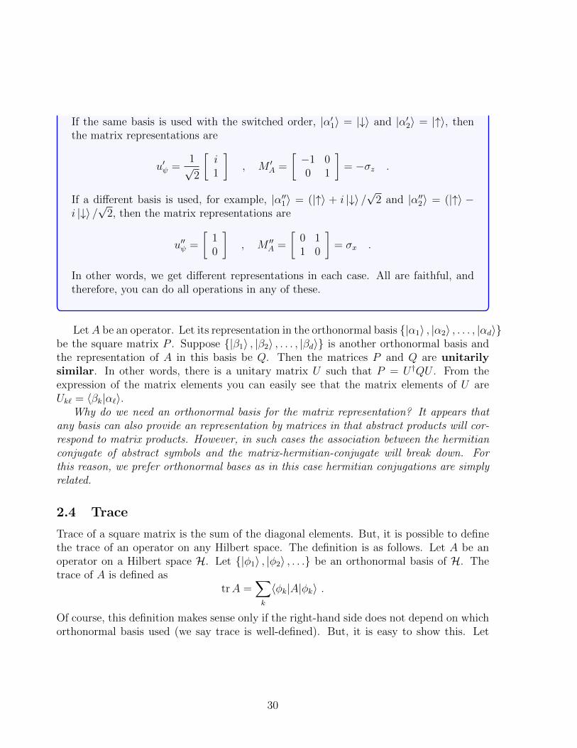
If the same basis is used with the switched order, |α′1〉 = |↓〉 and |α′2〉 = |↑〉, thenthe matrix representations are
u′ψ =1√2
[i1
], M ′
A =
[−1 00 1
]= −σz .
If a different basis is used, for example, |α′′1〉 = (|↑〉 + i |↓〉 /√
2 and |α′′2〉 = (|↑〉 −i |↓〉 /
√2, then the matrix representations are
u′′ψ =
[10
], M ′′
A =
[0 11 0
]= σx .
In other words, we get different representations in each case. All are faithful, andtherefore, you can do all operations in any of these.
LetA be an operator. Let its representation in the orthonormal basis {|α1〉 , |α2〉 , . . . , |αd〉}be the square matrix P . Suppose {|β1〉 , |β2〉 , . . . , |βd〉} is another orthonormal basis andthe representation of A in this basis be Q. Then the matrices P and Q are unitarilysimilar. In other words, there is a unitary matrix U such that P = U †QU . From theexpression of the matrix elements you can easily see that the matrix elements of U areUk` = 〈βk|α`〉.
Why do we need an orthonormal basis for the matrix representation? It appears thatany basis can also provide an representation by matrices in that abstract products will cor-respond to matrix products. However, in such cases the association between the hermitianconjugate of abstract symbols and the matrix-hermitian-conjugate will break down. Forthis reason, we prefer orthonormal bases as in this case hermitian conjugations are simplyrelated.
2.4 Trace
Trace of a square matrix is the sum of the diagonal elements. But, it is possible to definethe trace of an operator on any Hilbert space. The definition is as follows. Let A be anoperator on a Hilbert space H. Let {|φ1〉 , |φ2〉 , . . .} be an orthonormal basis of H. Thetrace of A is defined as
trA =∑k
〈φk|A|φk〉 .
Of course, this definition makes sense only if the right-hand side does not depend on whichorthonormal basis used (we say trace is well-defined). But, it is easy to show this. Let
30
{|α1〉 , |α2〉 , . . .} be another orthonormal basis of H. Then,∑`
〈α`|A|α`〉 =∑`
〈α`|1A|α`〉
=∑`,k
〈α`|φk〉〈φk|A|α`〉
=∑`,k
〈φk|A|α`〉〈α`|φk〉
=∑k
〈φk|A1|φk〉
= trA .
This shows that the trace is well-defined.The definition also conforms well with the matrix traces. If we form matrix repre-
sentation of A in the orthonormal basis {|φ1〉 , |φ2〉 , . . .}, then the matrix elements areAkj = 〈φk|A|φj〉. The diagonal elements are Akk and
trA =∑k
Akk ,
which shows that the trace is equal to the matrix-trace of the matrix representation. Ofcourse, the previous theorem above shows that the trace does not depend on the basis usedfor forming the matrix representation.
Below, we are going to show some properties of the trace function.
• trAB = trBA.
As this is a fundamental result, we prove it. Let {|φ1〉 , |φ2〉 , . . .} be an orthonormalbasis. Then
trAB =∑k
〈φk|AB|φk〉
=∑k
〈φk|A1B|φk〉
=∑k,`
〈φk|A|φ`〉〈φ`|B|φk〉
=∑k,`
〈φ`|B|φk〉〈φk|A|φ`〉
=∑`
〈φ`|B1A|φ`〉
= trBA .
31

• The rule above can be extended to many products
trABC = trCAB = trBCA ,
trABCD = trDABC = · · · .
WARNING
Some people may think that the rule is “everything commutes under trace”,which is not true. As a result, trABC 6= trACB. For example, check thefollowing by explicitly computing both sides.
trσxσyσz 6= trσxσzσy .
• tr |α〉 〈β| = 〈β|α〉.This is also an interesting result because it looks similar to the rule for operators,except that there is no trace sign on the right-hand side. This is another place wherethe Dirac notation becomes useful. The proof is straightforward from the definition.Let {|φ1〉 , |φ2〉 , . . .} be an orthonormal basis. Then,
tr |α〉 〈β| =∑k
〈φk|α〉〈β|φk〉
=∑k
〈β|φk〉〈φk|α〉
= 〈β|1|α〉 = 〈β|α〉 .
We can extend this result to more complicated cases; a few are written below.
tr |α〉 〈β|γ〉 〈δ| = 〈δ|α〉〈β|γ〉 = tr |γ〉 〈δ|α〉 〈β| ,trA |α〉 〈β| = 〈β|A|α〉 = tr |α〉 〈β|A .
• trABA−1 = trB, or similar matrices have same trace.
• trA is equal to the sum of the eigenvalues of A with the multiplicities counted. Ifthe operator is not “diagonalizable” and we have a finite dimensional Hilbert space,then the eigenvalues must be found from the roots of the characteristic polynomial,pA(x) = det(xI − MA), where MA is any matrix representation of A. In this case,second highest term of the characteristic polynomial gives the trace. If the dimensionis d, then
pA(x) = xd − (trA)xd−1 + · · ·+ (−1)d detA .
32
3 Spectral Theory
3.1 Eigenvalue Equation
Let A be an operator. We say that the scalar number λ is an eigenvalue of A if the equationA |ψ〉 = λ |ψ〉 has a non-zero solution for the ket |ψ〉. (The trivial solution |ψ〉 = 0 willalways satisfy the equation for any value of λ. We exclude this case.) The solution |ψ〉 iscalled the corresponding eigenvector (or eigenket, eigenstate, eigenfunction etc.)
• Note that if |ψ〉 is an eigenvector of A having eigenvalue λ, then for any non-zero scalarc, the ket c |ψ〉 is also an eigenvector with the same eigenvalue.
• Moreover, if |ψ1〉 , |ψ2〉 , . . . , |ψm〉 are eigenvectors of A having the same eigenvalue λ,then any superposition of these is an eigenvector with the same eigenvalue. For thisreason, it might be more appropriate to talk about the eigen-subspace which is thesubspace spanned by all eigenvectors having the same eigenvalue λ. Therefore, anyvector in that space is an eigenvector of A.
The dimension of this eigen-subspace is called the degeneracy of the eigenvalue λ.Degeneracy is the maximum number of linearly independent vectors you can find inthat eigen-subspace. In solving the eigenvalue problem, it is sufficient to determine onlysuch a set of linearly independent eigenvectors (once you know these, you can find allpossible eigenvectors with that eigenvalue). You can choose such vectors in any wayyou want, but in some cases it is advantageous to choose them as an orthonormal set.
• IfA is a d×d square matrix, then all eigenvalues ofA are the roots of the characteristicpolynomial
p(λ) = det(λI − A) .
This is a polynomial with degree d. Therefore it has d roots when the multiplicitiesare counted. If A is an abstract operator, then the eigenvalues of A are identical tothe eigenvalues of any of its matrix representation MA.
• If p(λ) = (λ − λ1)m1(λ − λ2)
m2 · · · (λ − λk)mk , then the eigenvalue λj has algebraic
multiplicity mj. Normally, we expect that the degeneracy of the eigenvalue is thesame as the multiplicity (i.e., λj has degeneracy mj). If this is the case then youcan form a basis where basis vectors are chosen from the eigenvectors (this is becausem1 +m2 + · · ·+mk = d is equal to the dimension of the Hilbert space).
But there are (rare) exceptions to this rule. The simplest example is the matrix
A =
[0 10 0
].
The characteristic polynomial is p(λ) = λ2 and therefore λ1 = 0 is a double root(m1 = 2). However, A has only one eigenvector having 0 eigenvalue, i.e., degeneracy
33
is 1 (Check this). Therefore, in this special case, you cannot find a basis chosen fromthe eigenvectors of A.
• If the dimension of the Hilbert space is ∞, then there are operators that do not haveany eigenvalue at all (the creation operator we meet in Harmonic oscillator problem isone such example).
• For most of the operators that we meet in quantum mechanics, namely hermitian andunitary operators (in general for all normal operators), the general rule applies: Thedegeneracy of an eigenvalue is equal to its multiplicity and we can find a basis from theeigenvectors. Moreover, we can choose that basis to be orthonormal. The basic resultthat we will use (but we will not prove) is the following. (Remember: An operator N isnormal if it commutes with its hermitian conjugate: NN † = N †N . Normal operatorsis a large class of operators which include hermitian and unitary operators.)
Theorem. Let N be a normal operator in a Hilbert space H with dimH = d.Then there is an orthonormal basis {|ϕ1〉 , |ϕ2〉 , . . . , |ϕd〉} of H where each |ϕk〉is an eigenvector of N .
– Let us investigate some immediate conclusions. Let N and |ϕk〉 be as in thetheorem above and let λk be the corresponding eigenvalues i.e., N |ϕk〉 = λk |ϕk〉.Since these vectors form an orthonormal basis we have the expansion of identity,1 =
∑k |ϕk〉 〈ϕk|. Now, expanding N = N1 we get
N =d∑
k=1
λk |ϕk〉 〈ϕk| . (5)
This is called the spectral decomposition of the operator N (its expansion interms of its eigenvalues and eigenvectors).
– The hermitian conjugate N † is then
N † =d∑
k=1
λ∗k |ϕk〉 〈ϕk| .
This shows that |ϕk〉 is also an eigenvector of N †, but with complex conjugatedeigenvalue λ∗k (i.e., N † |ϕk〉 = λ∗k |ϕk〉).
– From the two expansions above we get
NN † = N †N =d∑
k=1
|λk|2 |ϕk〉 〈ϕk| ,
34
which implies that N and N † commute ([N,N †] = 0). (Therefore, the converseof the theorem is valid: if an orthonormal basis can be formed from eigenvectorsof an operator, then the operator must be normal.)
– If N is hermitian, then the equation N = N † gives λk = λ∗k. In other words, alleigenvalues are real numbers. (Therefore, hermitian operators are those normaloperators which have only real eigenvalues.)
– If N is unitary, then the equation NN † = 1 gives |λk| = 1. In other words,the eigenvalues have modulus 1. You can then find an angle θk such that λk =eiθk . (Same comment: Unitary operators are those normal operators which haveeigenvalues with modulus 1 only.)
– If a normal operator N is neither hermitian nor unitary, then it should have acomplex eigenvalue and an eigenvalue with modulus different from 1.
– If N has the spectral decomposition given in (5), then the matrix representationof N in the orthonormal basis {|ϕ1〉 , |ϕ2〉 , . . . , |ϕd〉} is
MN =
λ1 0 · · · 00 λ2 · · · 0...
.... . .
...0 0 · · · λd
,
which is a diagonal matrix. In short, for every normal operator there is arepresentation where the operator is represented by a diagonal matrix. (More ondiagonalization below.)
• We can extend the theorem above for a commuting set of normal operators. In thiscase, we can find common eigenvectors of all operators. And we can also form anorthonormal basis from these eigenvectors.
Theorem. If A,B, . . . , Z are a mutually commuting set of normal operators(i.e., [A,B] = [A,C] = · · · = [Y, Z] = 0) on H, then there is an orthonormalbasis {|ϕ1〉 , |ϕ2〉 , . . . , |ϕd〉} of H where each |ϕk〉 is an eigenvector of all theoperators in that set. (i.e., A |ϕk〉 = αk |ϕk〉, B |ϕk〉 = βk |ϕk〉, etc.)
3.2 Diagonalization
Suppose that A is a d × d normal matrix. Let λk be its eigenvalues and ϕk be the eigen-vectors which form an orthonormal basis. We can use the eigenvectors to show that A isunitarily similar to a diagonal matrix as follows.
35
First, construct a d×d unitary matrix U by arranging the column vectors ϕ1, ϕ2, . . . , ϕdside by side.
U =
[ϕ1 ϕ2 · · · ϕd↓ ↓ · · · ↓
]Now, U is obviously unitary since the columns form an orthonormal basis. Next, wecompute the matrix product AU . By the properties of the matrix product, you can seethat different columns “do not mix”. The result will be same matrix U but this time eachcolumn is multiplied with a number. To be precise, all elements of column k is multipliedby the eigenvalue λk. In other words,
AU =
[Aϕ1 Aϕ2 · · · Aϕd↓ ↓ · · · ↓
]=
[λ1ϕ1 λ1ϕ2 · · · λdϕd↓ ↓ · · · ↓
]By the properties of the matrix product, you can see that the final matrix can be writtenas a product UD where D is a diagonal matrix.
AU =
[ϕ1 ϕ2 · · · ϕd↓ ↓ · · · ↓
]λ1 0 · · · 00 λ2 · · · 0...
.... . .
...0 0 · · · λd
As a result, we have the matrix equation AU = UD where U is unitary and D is diagonal.Taking a product with U † from left we get U †AU = D. In other words, A is unitarily similarto a diagonal matrix. This process of finding D is called diagonalization. Diagonalization isactually equivalent to solving the eigenvalue problem, since once you have found a unitarymatrix U such that U †AU is diagonal, then you know that the columns of U are theeigenvectors.
It should be obvious that if A is similar to a diagonal matrix D, then the diagonalelements of D are eigenvalues of A (which are also the eigenvalues of D). Diagonalizationis very important since certain computations can be done easily with the diagonal matrices(for example, computing an arbitrary function of an operator, as we will see below). Whatwe have shown above is this: Every normal matrix is unitarily similar to a diagonal matrix.The opposite is also true: If A is unitarily similar to a diagonal matrix then A must benormal (show this).
There are other ways of constructing the diagonal and unitary matrices as definedabove. For example, we could have started with the spectral decomposition of A as A =∑d
k=1 λkϕkϕ†k with the obvious translation between kets and bras and column and row
vectors. Let ek be the column vector whose kth element is 1 and all the rest is 0. Then,{e1, e2, . . . , ed} is the standard orthonormal basis of d × 1 column matrices. Let D =∑
k λkeke†k. You can easily check that D is a diagonal matrix with diagonal elements being
36

equal to the eigenvalues. Define U as U =∑
k ϕke†k. Check that U is unitary (Remember
that one of the equivalent descriptions of unitary operators says that U converts oneorthonormal basis into another). Since Uek = ϕk, together with the associated equationfor bras we get A = UDU †. This then gives U †AU = D.
3.3 Projections
We say that P is a projection operator if
(i) P is hermitian, (P † = P ), and
(ii) P 2 = P .
• Show that if P is a projection, then 1 − P is also a projection (1 − P is called thecomplementary projection). Show also that
P (1− P ) = (1− P )P = 0 .
• Show that the eigenvalues of projection operators are either 0 or 1.
• Let P and Q be two projections which commute, i.e., PQ = QP . Show that PQ andP +Q− PQ are also projections.
• Let |ϕ〉 be a normalized ket. Show that P = |ϕ〉 〈ϕ| is a projection operator.
• Let {|ϕ1〉 , |ϕ2〉 , . . . , |ϕk〉} be an orthonormal set (but it does not need to be a basisfor the whole Hilbert space). Show that P =
∑kj=1 |ϕj〉 〈ϕj| is a projection operator.
The projection operators correspond to the geometric operation of orthogonal projec-tion on to a subspace as follows. Let V be a subspace of the Hilbert space H. Let |ψ〉 bean arbitrary vector in the Hilbert space. Our problem is to find the projection of |ψ〉 onthe subspace V . To be precise, we would like to find two vectors
∣∣ψ‖⟩ and |ψ⊥〉 such that
. |ψ〉 =∣∣ψ‖⟩+ |ψ⊥〉
.∣∣ψ‖⟩ is “parallel” to the subspace V (in other words,
∣∣ψ‖⟩ ∈ V) and
. |ψ⊥〉 is perpendicular to every vector in V .
(This problem is also equivalent to the problem of finding a vector∣∣ψ‖⟩ ∈ V such that the
distance∥∥ψ − ψ‖∥∥ is minimum.)
37

Such a decomposition is unique. Also the map |ψ〉 →∣∣ψ‖⟩ is linear. Therefore we can
express it with a linear operator P , i.e.,∣∣ψ‖⟩ = P |ψ〉.
If |α〉 is already in the subspace V , we should have P |α〉 = |α〉. This implies thatfor any arbitrary |ψ〉 we have P 2 |ψ〉 = P
∣∣ψ‖⟩ =∣∣ψ‖⟩ = P |ψ〉. Therefore, the operator
satisfies P 2 = P .Property of being hermitian is related to the fact that the projection is orthogonal.
First note that, for two arbitrary vectors |ψ〉 and |φ〉, their inner product can be writtenas 〈ψ|φ〉 = 〈ψ‖|φ‖〉 + 〈ψ⊥|φ⊥〉, which follows from the orthogonality of the parallel andorthogonal components. By the same reasoning, we have 〈ψ‖|φ〉 = 〈ψ‖|φ‖〉 = 〈ψ|φ‖〉.Expressing the last equality in terms of the operator P , we get P † = P †P = P . Hence,P is a projection operator by the meaning defined at the beginning. (The opposite is alsotrue. If P is an operator satisfying P 2 = P = P †, then P corresponds to an orthogonalprojection to some subspace V. In that case, V is the eigensubspace of P corresponding tothe eigenvalue 1.)
Note that |ψ⊥〉 can be obtained by the complementary projection |ψ⊥〉 = (1− P ) |ψ〉.Here, 1 − P maps every vector to its component perpendicular to V . The subspace ofvectors which are orthogonal to every vector in V is denoted by V⊥ and is called as theothogonal complement of V . In other words, |α〉 ∈ V⊥ if and only if |α〉 is orthogonal toevery vector in V . For example, if V is the xy-plane in R3, then V⊥ is the z axis. As aresult, if P is projection onto V , then 1− P is the projection operator onto V⊥.
Several relations between projection operators can easily be interpreted in terms of thesubspaces they project onto.
• If P is a projection onto V , then every vector in V is an eigenvector of P with eigenvalue1 and every vector in V⊥ is an eigenvector with eigenvalue 0. If {|ϕ1〉 , |ϕ2〉 , . . . , |ϕk〉}is a basis for V (in which case we have k = dimV=degeneracy of eigenvalue 1) then Pcan be expressed as P =
∑kj=1 |ϕj〉 〈ϕj|. The final expression does not depend on the
orthonormal basis used for the subspace.
• In particular, if |ϕ〉 is a normalized vector, then P = |ϕ〉 〈ϕ| is a one-dimensionalprojection onto the 1D subspace spanned by |ϕ〉. For any vector |ψ〉, P |ψ〉 = |ϕ〉 〈ϕ|ψ〉is the component of |ψ〉 parallel to |ϕ〉.
38

• if P is a projection operator, then trP is equal to the dimension of the subspace thatP projects to. In particular, tr |ψ〉 〈ψ| = 1 for a normalized |ψ〉.
• If two projections P and Q satisfy PQ = 0, then the subspaces they project to aredisjoint and orthogonal to each other.
• If the two projections satisfy PQ = P , then the subspace associated with P is inside(a subset of) the subspace associated by Q. (Show this.)
• If two projections P and Q do not commute, PQ 6= QP , then it means that theirsubspaces are “making a non-trivial angle” with each other.
• If two projections P and Q project onto subspaces V and W respectively, and theycommute, PQ = QP , then the subspaces have some nice properties. First, note thatyou can find a common orthonormal basis formed from eigenvectors of both P and Q.Using such a basis, you can see that PQ is a projection onto the intersection V ∩W .Moreover, P +Q−PQ = 1− (1−P )(1−Q) is a projection for the subspace V +W .
39

EXAMPLE
If P is the projection onto xy plane and Q onto xz plane, then PQ is theprojection onto x axis and P + Q − PQ is projection onto the whole space R3
(which means P +Q− PQ = 1 is the identity).
We will use the projection operators as follows: Let A be a normal operator (usuallyhermitian). Let λ1, λ2, . . . , λs denote its distinct eigenvalues (if j 6= k then λj 6= λk). Letthe eigenvalue λj has degeneracy dj. We know that we can find an orthonormal basis{|ϕjb〉} where j index takes values 1, 2, . . . , s and denotes the eigenvalue and the b indextakes values 1, 2, . . . , dj and just labels the different eigenvectors corresponding to thesame eigenvalue, λj. In other words, for any j, the vectors |ϕj1〉 , |ϕj2〉 , . . . ,
∣∣ϕjdj⟩ span theeigensubspace of A corresponding to the eigenvalue λj. Define the projection operators Pjfor each j as
Pj =
dj∑b=1
|ϕjb〉 〈ϕjb| .
Then, Pj is a projection operator to the eigensubspace for λj. Since, different eigensub-spaces are orthogonal we have PjPk = PkPj = 0 for j 6= k (show this). Moreover, by theexpansion of identity we have 1 = P1 + P2 + · · · + Ps. The spectral decomposition of Athen can be written as
A =∑jb
λj |ϕjb〉 〈ϕjb| =∑j
λjPj .
This is also called the spectral decomposition of A. It is sometimes better to use thisexpression than the decomposition in (5), which are expressed in terms of the eigenvectors.One of the reasons is this: If an eigenvalue λj is degenerate then there is some arbitrarinessin choosing the kets {|ϕj1〉 , . . . ,
∣∣ϕjdj⟩}. However, the corresponding projection operatorPj onto that eigensubspace does not depend on that choice. Whenever you do not wantto compute the individual eigenvectors, then the spectral decomposition by projectionoperators is preferable.
The first theorem can then be phrased as follows: If N is a normal operator and {λj}are its distinct eigenvalues, then there is a complete set of orthogonal projection operatorsPj such that
PjPk = 0 (if j 6= k) ,∑j
Pj = 1 ,
N =∑j
λjPj .
40
Moreover, these projection operators are unique.
Problem 6. Let A be a normal operator whose only eigenvalues are +1 and −1.Show that the corresponding projection operators P+ and P− are
P+ =1 + A
2, P− =
1− A2
.
Show also that P+ + P− = 1 and P+P− = P−P+ = 0.Problem 7. Let A be a normal operator having only three distinct eigenvalues λ1,λ2 and λ3. Show that
P1 =(A− λ21)(A− λ31)
(λ1 − λ2)(λ1 − λ3)is the projector for the eigen-subspace corresponding to λ1. What are the otherprojectors?
4 Functions of Operators
4.1 Functions of Normal Operators
We would like to define some operator valued functions of operators. There are someexamples that are met frequently in applications like the exponential function: exp(A)where A is an operator. There are two different ways of defining such functions, each hasits own problems. As such functions are needed mostly with normal operators, we willadopt the following definition.
Let f(t) be a function of a complex number t. We place no restrictions on the type ofthe function. It does not need to be analytic. It does not need to be defined everywhere.It can be discontinuous, etc. Let A be a normal operator with spectral decomposition
A =∑k
λk |ϕk〉 〈ϕk| .
Then, we define f(A) as the following operator
f(A) =∑k
f(λk) |ϕk〉 〈ϕk| . (6)
If f(t) is not defined everywhere, then we require that the eigenvalues of A are in thedomain of f in order to compute f(A). Below, we will see some conclusions that we drawfrom that definition.
41
• The definition does not depend on how the eigenkets of A are chosen. Especially, ifA =
∑′j λjPj where Pj are projections onto the eigensubspace corresponding to the
eigenvalue λj and prime indicates that the sum is taken over distinct eigenvalues, thenf(A) =
∑′j f(λj)Pj. In particular, if A and B are unitarily similar by A = U †BU ,
then f(A) = U †f(B)U .
• If A is normal, then f(A) is normal. If A |ϕ〉 = λ |ϕ〉 (i.e., |ϕ〉 is an eigenket of A witheigenvalue λ) then f(A) |ϕ〉 = f(λ) |ϕ〉. In other words, |ϕ〉 is also an eigenket of f(A)but with eigenvalue f(λ). In conclusion, evaluation of function f does not change theeigenvectors of the operator, it just changes its eigenvalues.
• If several functions satisfy a particular relationship among them, then same relationshipwill continue to be satisfied when the argument is replaced by the same operator. Forexample if f(t)g(t) + h(t) = k(t) then f(A)g(A) + h(A) = k(A). Example: eiA =cosA+ i sinA.
• The rule above is not valid in relations where functions of two different operators arepresent. The most famous one is this: We know et1et2 = et1+t2 for every complexnumber t1 and t2. But the corresponding relation for operators is not valid. There arecases where eAeB 6= eA+B. In most of these cases we also have eAeB 6= eBeA, etc. Butif the arguments are the same operator, the rule above applies (it is easy to see thisfrom the definition). For example: et1Aet2A = e(t1+t2)A.
• In particular for the powers An = AA · · ·A, which is the product of n A’s. In thatcase we have
An =∑k
λnk |ϕk〉 〈ϕk| ,
which can easily be seen to be true. But this expression can be seen as a special casefor the function f(t) = tn.
In some cases, it is appropriate to define 0th power function as f(t) = t0 = 1. (If t 6= 0,this is correct. But if t = 0, the power is undefined. We just define f(0) = 1 for thisspecial case.) In that case, we have
A0 =∑k
λ0k |ϕk〉 〈ϕk| =∑k
|ϕk〉 〈ϕk| = 1 .
This rule can be considered as a formal definition to be used in the power seriesexpansions
f(t) =∞∑n=0
cntn = c0 + c1t+ c2t
2 + · · ·
As a result, we will expand f(A) as
f(A) =∞∑n=0
cnAn = c01 + c1A+ c2A
2 + · · ·
42

• The power −1 can be considered as inverse. For f(t) = t−1, we have
A−1 =∑k
1
λk|ϕk〉 〈ϕk| .
If all eigenvalues are non-zero, then A−1 defined above is well-defined. You can checkthat A−1 given above is indeed the inverse of A, i.e., check that A−1A = AA−1 = 1.
• If A is a diagonal matrix,
A =
λ1 0 · · · 00 λ2 · · · 0...
.... . .
...0 0 · · · λd
,
then the eigenvectors of A are the standard basis vectors. The definition above thenimplies
f(A) =
f(λ1) 0 · · · 0
0 f(λ2) · · · 0...
.... . .
...0 0 · · · f(λd)
,
• If A is unitarily similar to a diagonal matrix as A = UDU †, where D is diagonal andU is unitary, then f(A) = Uf(D)U † where f(D) is as computed above. Therefore, ifyou have diagonalized a matrix, then it is easy to compute the function of that matrix.
• Suppose that A is an operator whose only eigenvalues are ±1, then
f(A) = f(1)P+ + f(−1)P−
= f(1)1 + A
2+ f(−1)
1− A2
=f(1) + f(−1)
21 +
f(1)− f(−1)
2A
where we have used a previously computed expression for projection operators ontothe eigensubspaces of A. The most commonly encountered case is
eiθA = cos θ1 + i sin θA .
• Let λ1, λ2, . . . , λs be all of the distinct eigenvalues of a normal operator A. Considerthe polynomial
p(t) = (t− λ1)(t− λ2) · · · (t− λs) =s∏j=1
(t− λj) .
43

Then you can see that p(A) = 0. This is usually called the minimal polynomial of A(it is the smallest degree polynomial p such that p(A) = 0). For each eigenvalue λi,define a new polynomial pi(t) as follows
pi(t) =
∏j 6=i(t− λj)∏j 6=i(λi − λj)
=(t− λ1) · · · (t− λi−1)(t− λi+1) · · · (t− λs)
(λi − λ1) · · · (λi − λi−1)(λi − λi+1) · · · (λi − λs).
Note that pi(t) is a factor of p(t) which misses only the root at λi. Check that pi(λi) = 1and for all other j we have pi(λj) = 0. Using the spectral decomposition, it is theneasy to see that
Pi = pi(A) ,
is the projection operator onto the eigensubspace corresponding to eigenvalue λi.(Check: p(t) divides pi(t)pj(t) when i 6= j. Therefore, PiPj = 0.)
Problem 8. Suppose that A has eigenvalues −1, 0 and +1 only. Compute thecorresponding projection operators P−1, P0 and P1 in terms of A.
Problem 9. The x-component of angular momentum for the quantum number` = 1 can be written in a particular matrix representation as
Jx =1√2
0 1 01 0 10 1 0
.
Check that Jx has eigenvalues −1, 0 and +1. Compute the corresponding pro-jection operators P−1, P0 and P1. In this case, each of these are 1D projectors.Take an arbitrary vector ψ (almost anything will do). Compute P−1ψ, P0ψ andP1ψ. From these, find the normalized eigenvectors of Jx.
Now, we will see some scattered standard results that are sometimes useful.
• Every unitary matrix can be expressed as the exponential of an anti-hermitian operator.Let U be a unitary operator. Then, U has some spectral decomposition as
U =∑k
eiθk |ϕk〉 〈ϕk| ,
where eiθk are the eigenvalues and |ϕk〉 are the eigenkets forming an orthonormal basis.Define an operator A as A =
∑k θk |ϕk〉 〈ϕk|. Then A is a hermitian operator since
44

each θk are real. It is then easy to see that
U = eiA .
Here iA is called an anti-hermitian operator, it changes sign under hermitian conjuga-tion, (iA)† = −iA. The operator A is not unique. For example, in the constructionabove you can add to each θk an integer multiple of 2π. In each case, you will get adifferent operator A, but eiA will still be equal to U .
• If U(t) are unitary operators depending on a real parameter t such that U(t1)U(t2) =U(t1 + t2), then there is a unique hermitian operator A such that U(t) = eitA.
4.2 Alternative definition of functions of operators
The previous definition of function of operators, in other words, defining f(A) from thespectral decomposition of A
A =∑k
λkPk −→ f(A) =∑k
f(λk)Pk .
has some nice and some bad features. It is good that the function f could be anything.It does not need to be analytic; it does not need to be continuous; it does not even haveto be defined for all complex or real numbers. It is only necessary that the eigenvaluesof the operator A needs to be in the domain of the function so that f(A) can be defined.So, for example,
√A can be defined if all eigenvalues of A are real and positive. Its main
shortcoming is that A has to be a normal operator so that it has a spectral decomposition.Sometimes, we may need to use some functions of non-normal operators as well. As
the above approach cannot be used now, we need another definition. This one is basedon the analyticity of functions. Let f(z) be an analytic function of the complex numberz. This means that, we can do a Taylor series expansion of f at any interior point it isdefined. For simplicity, let’s expand it around 0,
f(z) =∞∑n=0
cnzn = c0 + c1z + c2z
2 + · · ·
Then, for any operator A, we define
f(A) =∞∑n=0
cnAn = c01 + c1A+ c2A
2 + · · ·
where we use the convention A0 = 1 for any A. This and the previous definition for a“function of an operator” agrees with each other when the operators are normal and thefunctions are analytic. You can think of this as a way of extending the previous definitionto non-normal operators.
45
The most frequently appearing function is the exponential function. For any operatorA, we have
eA = 1 + A+A2
2+ · · · =
∞∑n=0
An
n!.
Some of the familiar properties of the exponential keep holding in the operator case, butsome don’t. Let t be a complex number considered as a free variable. The relation
d
dtetA = AetA = etAA
can be shown easily from the power series expansion. Consequently, the following differen-tial equations for an operator valued function F = F (t) of parameter t, has the followingobvious solution provided that the operator X is independent of t.
d
dtF (t) = XF (t) −→ F (t) = etXF (0) ,
d
dtF (t) = F (t)X −→ F (t) = F (0)etX ,
If A and B are operators that do not commute with each other, then eAeB 6= eA+B.But, sometimes we would like to express eAeB as a single exponential. The associatedrelation, usually known as Baker-Campbell-Hausdorff formula, can be derived by using theseries expansion of the exponential function. But, in order to follow the powers in thederivation easily, we usually introduce a complex parameter such as t. Basically we have
etAetB = eC(t)
where
C(t) = t(A+B) +t2
2[A,B] +
t3
12([A, [A,B]] + [B, [B,A]) + · · ·
is an infinite symbolic series. In general we can say the following about this expansion:the coefficient of tn is a sum of terms formed by n− 1 commutators of n of the A and Bs.There is no simple formula for the nth term. In some simple cases, we can write down anexact expression for C(t). The obvious case is the one when A and B commute with eachother, in which case only the 1st order term of C(t) is present.
AB = BA =⇒ etAetB = et(A+B) .
Another useful case is when the commutator [A,B] commutes with both A and B, in whichcase C(t) has only 1st and 2nd order terms.
[A,B] commutes with A and B =⇒ etAetB = et(A+B)+ t2
2[A,B] .
46

Problem 10. The ladder operators a and a† that appear in the treatment ofharmonic oscillator and bosons satisfy [a, a†] = 1. Let λ and µ be two complexnumbers. Find the numbers c1 and c2 in the following identity.
eλaeµa†
= c1eλa+µa† = c2e
µa†eλa .
Problem 11. Let x be the position and p be the momentum operator, which satisfy[x, p] = i~. For constant a, the unitary operator
T (a) ≡ exp
(− i~pa
)is called the translation operator, and for constant q,
B(q) ≡ exp
(i
~xq
)can be called as the boost operator. Show that
T (a)B(q) = cB(q)T (a)
for some number c and compute the value of c.
5 Positive Operators
We say that an operator A is positive semidefinite if all of its expectation values are non-negative: 〈ψ|A|ψ〉 ≥ 0 for any vector |ψ〉. In this case we say, A ≥ 0. Note that, thedefinition implies that all expectation values are also real numbers (so that you can claimthem to be positive). As a result, when we say A is positive semidefinite, then we alsoimply that it is a hermitian operator.
A closely related concept is positiveness. We say that an operator A is positive definiteif all of its expectation values in non-zero states are positive numbers: In other words,〈ψ|A|ψ〉 > 0 for any non-zero vector |ψ〉. In this case we say A > 0.
The terminology given above is quite standard in mathematics, but physicists mightuse some alternative expressions. Some people use positive or non-negative definite forpositive semidefiniteness, and they use strictly positive for positive definiteness. In anycase, if we use ≥ and > signs correctly, no confusion can arise.
A ≥ 0 if 〈ψ|A|ψ〉 ≥ 0 for all |ψ〉 ,A > 0 if 〈ψ|A|ψ〉 > 0 for all |ψ〉 6= 0 .
47
The definitions above are quite useful for proving some results (like proving the positivedefiniteness of B†B), but there is a much more simpler description of positive definitenessin terms of the eigenvalues. Let A be a hermitian operator and let A =
∑k λk |ϕk〉 〈ϕk| be
its spectral decomposition. Then, we have the following result
A ≥ 0 if λk ≥ 0 for all k ,
A > 0 if λk > 0 for all k .
Showing the equivalence of these two approaches is left to you.If A is a positive semidefinite operator, A ≥ 0, then there is a unique, positive semidef-
inite operator√A satisfying A = (
√A)2. The square-root operator
√A can be obtained
from the spectral decomposition of A. If
A =∑j
λj |ϕj〉 〈ϕj| ,
then √A =
∑j
√λj |ϕj〉 〈ϕj| .
Problem 12. Let B be an arbitrary operator. Show that B†B ≥ 0.Problem 13. Let B be an arbitrary operator and let A ≥ 0. Show that B†AB ≥ 0.Problem 14. Show that the sum of positive semidefinite operators is positivesemidefinite. In other words, if Ai ≥ 0, then
∑iAi ≥ 0.
Problem 15. Let {|α1〉 , . . . , |αn〉} be a list of n vectors. The overlap matrix ofthese vectors is the n×n matrix whose matrix elements are defined as Sij = 〈αi|αj〉.Show that S is positive semidefinite, S ≥ 0. Show also that S > 0 if and only if thevectors {|α1〉 , . . . , |αn〉} are linearly independent.
5.1 Positive Definiteness for Matrices
It is of some interest to investigate positivity separately for matrices. For any positivedefinite matrix, since all eigenvalues are also positive, the trace and determinant are alsopositive.
A > 0 =⇒ trA =∑i
λi > 0 ,
A > 0 =⇒ detA =∏i
λi > 0 .
48

The similar relation holds obviously for positive semidefinite matrices with inequaltiesreplaced with ≥.
If A > 0, then all diagonal entries must be positive, Aii > 0. This is quite easy tosee because the diagonal entries can be expressed as an expectation value, Aii = 〈ei|A|ei〉where ei is the ith vector of the standard basis (remember, ei is the column vector withith entry equal to 1 and all other entries equal to 0). Again, this can be extended to thesemidefinite case in the same way: A ≥ 0 =⇒ Aii ≥ 0.
Let A be an n × n matrix. A submatrix of A is a matrix A′ obtained by selecting anumber of rows and columns in such a way that the selected row and column indices arethe same. Let the indices be i1, i2, . . . , ik which are all different. There is no problem withselecting them such that i1 < i2 < · · · < ik. Then, the k × k submatrix A′ correspondingto this choice of indices is given by A′αβ = Aiαiβ . For example for
A =
3 2i 1−2i 2 i
1 −i 4
A′ = [3] , A′′ =
[3 11 4
], (7)
A′ is a 1× 1 submatrix and A′′ is a 2× 2 submatrix of A. It is quite easy to see that anyexpectation value of a submatrix is also an expectation value of the original matrix. Asa result, all submatrices of a positive definite matrix should also be positive definite andsimilarly for the semidefiniteness:
if A′ is a submatrix of A :
{A ≥ 0 =⇒ A′ ≥ 0 ,A > 0 =⇒ A′ > 0 .
Note that the rule about the diagonal elements is just a special case of the submatrix rulebecause all diagonal elements are 1× 1 submatrices.
It is a straightforward to see that all submatrices of positive matrices have positivedeterminants. It appears that the converse also holds and this can be turned into a simpletest of positiveness. Let A be an n × n matrix. Let us consider n special submatricesdenoted by A(1), A(2), . . . , A(n) where A(k) is the k× k submatrix obtained from the first kindices.
A(1) = [A11] , A(2) =
[A11 A12
A21 A22
], A(3) =
A11 A12 A13
A21 A22 A23
A31 A32 A33
, · · · , A(n) = A .
Sylvester rule states that A is positive definite if and only if the determinants of thesesubmatrices are positive.
49

A > 0 ⇐⇒ detA(k) > 0 for all k = 1, 2, . . . , n .
Unfortunately, leftward implication is not valid for positive semidefinite variant of theabove.
Problem 16. Determine if the matrix A in Eq. (7) is positive definite by using theSylvester’s rule.Problem 17. Sylvester’s rule cannot be adopted to positive semidefinite case.Consider as an example a 3 × 3 diagonal matrix A with diagonal entries 1, 0,−1appearing in that order. Show that detA(k) ≥ 0 for all k = 1, 2, 3, but A � 0.Problem 18. Derive Schwarz inequality from the Sylvester rule for a 2× 2 overlapmatrix.
5.2 Lowner Partial Order
We can define an order (a partial order) between hermitian operators by using the positivityconcept. For two hermitian operators A and B, we say that A ≥ B if A − B ≥ 0. Thissatisfies the basic properties of order
. if A ≥ B and B ≥ C then A ≥ C,
. if A ≥ B and A ≤ B then A = B.
This order is called Lowner partial order. It is partial because it may not be possible tocompare any two operators. In other words, there can be operators A and B, such thatA � B and B � A.
EXAMPLE
Are the following operators comparable by Lowner partial order?
A =
[1 00 0
], B =
[0 00 1
].
50
5.3 Polar decomposition
For any operator A, it is possible to find positive semidefinite operators R and R′ and aunitary operator U such that
A = UR = R′U .
Such an expression is called the polar decomposition of A. This is quite similar to thepolar decomposition of a complex number z as z = reiθ where r ≥ 0. Remembering thatany unitary operator U can be expressed as U = eiT where T is a hermitian operator,the parallel between the operator case and the number case is almost perfect. Of course,in the operator case, U may not commute with R or R′; hence, there are two different“modulus” operators. Since the polar decomposition is sometimes useful, a small expositionis necessary.
From the definition, we can see that R and R′ operators can be expressed uniquely. Aswe have A†A = R2 and AA† = R′2, we can see that both operators are necessarily equalto the following squareroots
R =√A†A ,
R′ =√AA† .
If the operator A is invertible, then both R and R′ are invertible as well. In such a case,we can uniquely define U as
U = AR−1 = R′−1A .
Showing that both expressions give the same U is a bit tricky. To do this, we first defineU = AR−1. Then, it is easy to see that
U †U = R−1A†AR−1 = R−1R2R−1 = 1 ,
which shows that U is unitary. Next, we note that
R′2 = AA† = UR2U † = (URU †)2 .
Since URU † is positive definite and since the square-roots are unique, we see that thetwo square-roots of AA† are identical and hence R′ = URU †. This then shows thatR′U = UR = A, which completes the proof.
So, the polar decomposition is unique if A is invertible. If A is not invertible, thenthere are many possible choices for the unitary U , so U is not unique. But both modulusoperators will be unique even in this case.
Note that both modulus operators are similar to each other: R′ = URU †. Therefore,they have the same set of eigenvalues. Their non-zero eigenvalues (namely the nonzero
eigenvalues of both√AA† and
√A†A) are usually known as the singular values of A.
This is also closely related to the singular-value decomposition of matrices. Supposethat A is a matrix. Since R is a positive semidefinite matrix, it is unitarily similar to a
51
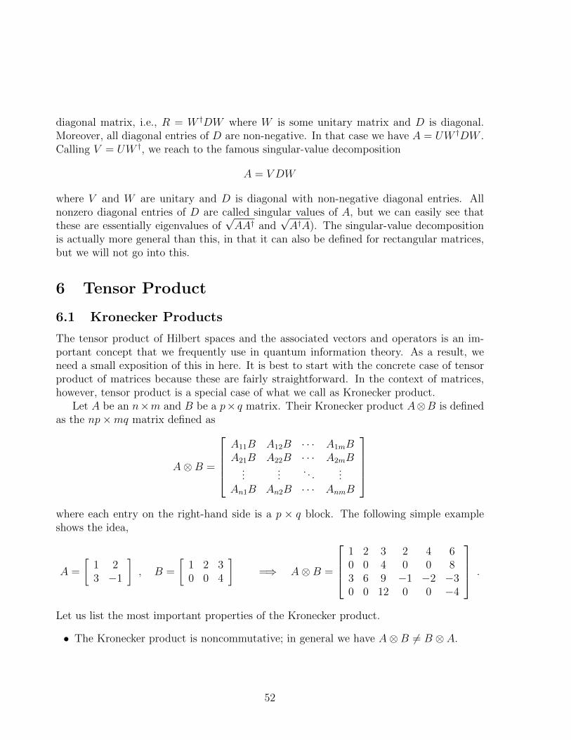
diagonal matrix, i.e., R = W †DW where W is some unitary matrix and D is diagonal.Moreover, all diagonal entries of D are non-negative. In that case we have A = UW †DW .Calling V = UW †, we reach to the famous singular-value decomposition
A = V DW
where V and W are unitary and D is diagonal with non-negative diagonal entries. Allnonzero diagonal entries of D are called singular values of A, but we can easily see thatthese are essentially eigenvalues of
√AA† and
√A†A). The singular-value decomposition
is actually more general than this, in that it can also be defined for rectangular matrices,but we will not go into this.
6 Tensor Product
6.1 Kronecker Products
The tensor product of Hilbert spaces and the associated vectors and operators is an im-portant concept that we frequently use in quantum information theory. As a result, weneed a small exposition of this in here. It is best to start with the concrete case of tensorproduct of matrices because these are fairly straightforward. In the context of matrices,however, tensor product is a special case of what we call as Kronecker product.
Let A be an n×m and B be a p× q matrix. Their Kronecker product A⊗B is definedas the np×mq matrix defined as
A⊗B =
A11B A12B · · · A1mBA21B A22B · · · A2mB
......
. . ....
An1B An2B · · · AnmB
where each entry on the right-hand side is a p × q block. The following simple exampleshows the idea,
A =
[1 23 −1
], B =
[1 2 30 0 4
]=⇒ A⊗B =
1 2 3 2 4 60 0 4 0 0 83 6 9 −1 −2 −30 0 12 0 0 −4
.
Let us list the most important properties of the Kronecker product.
• The Kronecker product is noncommutative; in general we have A⊗B 6= B ⊗ A.
52

• The Kronecker product is distributive over the matrix addition.
A⊗
(∑k
ckBk
)=∑k
ckA⊗Bk ,(∑k
dkAk
)⊗B =
∑k
dkAk ⊗B .
• If it is possible to take AA′ and BB′ products, then it is possible to take the (A ⊗B)(A′ ⊗B′) product and
(A⊗B)(A′ ⊗B′) = AA′ ⊗BB′ .
(Remember that AA′ product is possible if the number of columns of A is equal to thenumber of rows of A′.)
Most other properties of the Kronecker product can be derived by using the above. Forexample, let u and u′ be d × 1 column vectors and v and v′ are n × 1 column vectors.Then u⊗ v and u′⊗ v′ are dn× 1 column vectors. In that case, we have the inner productidentity
〈u⊗ v|u′ ⊗ v′〉 = 〈u|u′〉〈v|v′〉 ,
a relation which we will use in the abstract case.
6.2 Tensor Product of Hilbert Spaces
We would like to define a tensor product for abstract Hilbert spaces. The main need forthis comes from the necessity of describing composite quantum systems. If we have twodifferent systems A and B, then we have separate Hilbert spaces, say HA and HB, fordescribing the quantum states of these systems. Basically a vector |α〉A in HA gives astate of A and a vector |β〉B in HB gives a state of B. In a similar way, we should have anentirely different Hilbert space HAB for describing the states of the composite system AB.In particular, we would like to have a vector in HAB that describes the state of AB suchthat A is in state |alpha〉A and B is in state |β〉B. We will denote this state as |α〉A⊗|β〉B.We will also want to have this product ⊗ be such that superpositions of states in A or in Bcould also be equivalently described as superpositions of states in AB; hence distributivity.
We are not going to formally define the tensor product ⊗; instead we will describethe basic properties that it should satisfy. Using these properties, we can derive all otherproperties of the tensor product. Hence, suppose that HA and HB are any two Hilbertspaces (which may or may not be a state space of a quantum system). We will assume theexistence of another Hilbert space HAB = HA ⊗HB, called the tensor product of HA andHB. We will also define a tensor product operation on vectors such that
53

• For any |α〉A in HA and |β〉B in HB, the product |α〉A ⊗ |β〉B is a vector in HAB.
• The tensor product is distributive over addition,(∑i
ci |αi〉A
)⊗ |β〉B =
∑i
ci |αi〉 ⊗ |β〉B ,
|α〉A ⊗
(∑i
ci |βi〉A
)=∑i
ci |α〉 ⊗ |βi〉B .
• The inner product on HAB satisfies(A 〈α| ⊗ B 〈β|
)(|α′〉A ⊗ |β
′〉B)
= 〈α|α′〉A〈β|β′〉B
• HAB is generated by vectors of the form |α〉A ⊗ |β〉B. (Or, equivalently, HAB is thesmallest Hilbert space satisfying the properties above.)
Notation: The notation can become quite awkward in more complicated expres-sions. The subscript A in |· · · 〉A is usually put as a reminder that the vector belongsto HA. It can be dropped or indicated differently.
|α〉A ≡ |αA〉 ≡∣∣αA⟩ ≡ |α〉A ≡ |α〉 .
The tensor product can also be shown differently
|α〉A ⊗ |β〉B ≡ |α〉 ⊗ |β〉 ≡ |α⊗ β〉 ≡ |α〉 |β〉 ≡ |αβ〉 ≡ |αAβB〉 ≡ · · ·
An important detail that one should be careful is the order. So, |α〉A ⊗ |β〉B and|β〉B ⊗ |α〉A are different vectors. The latter is a vector in a different Hilbert spaceHB ⊗HA. This becomes especially important when the reminding labels are elimi-nated.
The same order is also used in bra’s,(|α〉 ⊗ |β〉
)†= 〈α| ⊗ 〈β| = 〈α⊗ β| .
For example, the inner product rule can be expressed more compactly as
〈α⊗ β|α′ ⊗ β′〉 = 〈α|α′〉〈β|β′〉 .
54

Let {|α1〉 , · · · , |αn〉} be an orthonormal basis for HA and {|β1〉 , · · · , |βm〉} be an or-thonormal basis forHB. We can see that the nm vectors of the form {|αi ⊗ βj〉}1≤i≤n, 1≤j≤mforms an orthonormal basis for HAB. First, we can see that these vectors are orthonormalfrom the rule about the inner-product
〈αi ⊗ βj|αk ⊗ β`〉 = 〈αi|αk〉〈βj|β`〉 = δikδj` .
Second, any vector |Ψ〉 in HAB is some kind of a superposition of tensor-product vectors,e.g., |Ψ〉 =
∑µ |φµ ⊗ χµ〉. As we can expand each |φµ〉 and |χµ〉 in the bases of their
respective Hilbert spaces, we can express |Ψ〉 as
|Ψ〉 =∑ij
cij |αi ⊗ βj〉 (8)
for some coefficients cij. This completes the proof that {|αi ⊗ βj〉}1≤i≤n, 1≤j≤m is an or-thonormal basis for HAB. This tells us that the space HAB has dimension nm. Or, if weexpress it in the general case we have
dim (HA ⊗HB) = dimHA dimHB .
If a vector can be expressed as the tensor product of two vectors, we call it a productvector, i.e., |Ψ〉 is a product vector if |Ψ〉 = |φ⊗ χ〉 for some |φ〉 and |χ〉. Any non-product vector is called entangled. The entangled states of a composite system occupya distinguished position in the interpretation of quantum mechanics. We will see thisdiscussion later.
The operators on tensor product spaces can also be expressed in terms of the operatorson the smaller spaces. Let P be an operator acting on HA and Q be an operator actingon HB. Then, by P ⊗Q we mean an operator acting on HAB such that
(P ⊗Q) |α⊗ β〉 = (P |α〉)⊗ (Q |β〉) .
Sometimes subscripts are used to remind us which spaces the operators act on,
(PA ⊗QB) |αA ⊗ βB〉 = PA |α〉A ⊗QB |β〉B .
Using the basic definition, we can check that the following properties hold for the tensorproduct of operators.
(P ⊗Q)(P ′ ⊗Q′) = PP ′ ⊗QQ′ ,〈α⊗ β|P ⊗Q|α′ ⊗ β′〉 = 〈α|P |α′〉〈β|Q|β′〉 ,
(P ⊗Q)† = P † ⊗Q† ,trP ⊗Q = trP trQ .
It is a simple exercise to show that any operator on HAB can be written as a sum of tensorproduct of operators.
To sum up, we can see a lot of similarities between the Kronecker product for matricesand the tensor product for abstract Hilbert spaces.
55

Problem 19. Let P be an operator on HA with eigenvalues λn and let Q bean operator on HB with eigenvalues µm. Show that P ⊗ Q has eigenvalues λnµm.What can you say about the eigenvalues? What can you say about their spectraldecompositions in the case P and Q are both normal?
56