NOVEL APPROACHES TO THE VISUALIZATION OF CELL SPECIFIC GENE

EXPRESSION PATTERNS

A DISSERTATION

SUBMITTED TO THE DEPARTMENT OF BIOENGINEERING

AND THE COMMITTEE ON GRADUATE STUDIES

OF STANFORD UNIVERSITY

IN PARTIAL FULFILLMENT OF THE REQUIREMENTS

FOR THE DEGREE OF

DOCTOR OF PHILOSOPHY

Chuba Benson Oyolu

December 2010

This dissertation is online at: http://purl.stanford.edu/gq062rg0666

© 2011 by Chuba Benson Odimegwu Oyolu. All Rights Reserved.

Re-distributed by Stanford University under license with the author.

ii

I certify that I have read this dissertation and that, in my opinion, it is fully adequatein scope and quality as a dissertation for the degree of Doctor of Philosophy.

Julie Baker, Primary Adviser

I certify that I have read this dissertation and that, in my opinion, it is fully adequatein scope and quality as a dissertation for the degree of Doctor of Philosophy.

Russ Altman

I certify that I have read this dissertation and that, in my opinion, it is fully adequatein scope and quality as a dissertation for the degree of Doctor of Philosophy.

Karl Deisseroth

Approved for the Stanford University Committee on Graduate Studies.

Patricia J. Gumport, Vice Provost Graduate Education

This signature page was generated electronically upon submission of this dissertation in electronic format. An original signed hard copy of the signature page is on file inUniversity Archives.

iii

II

© Copyright by Chuba Benson Oyolu 2010

All Rights Reserved

III

I certify that I have read this dissertation and that, in my opinion, it is fully adequate in scope and quality as a dissertation for the degree of Doctor of

Philosophy

(Julie C. Baker PhD) Principal Adviser

I certify that I have read this dissertation and that, in my opinion, it is fully adequate in scope and quality as a dissertation for the degree of Doctor of

Philosophy

(Russ B. Altman M.D. PhD)

I certify that I have read this dissertation and that, in my opinion, it is fully adequate in scope and quality as a dissertation for the degree of Doctor of

Philosophy

(Karl Deisseroth M.D. PhD)

Approved for the Stanford University Committee on Graduate Studies

IV

ABSTRACT

The fate of a cell is largely determined by the unique patterns of gene

expression found within it. Complex biological machinery exists within each

cell to manipulate chromatin state, and ultimately control gene expression.

Developmental processes such as cellular differentiation require very specific

chemical signals and environmental conditions. These serve as triggers to put

the chromatin modification schemes that produce the resultant patterns of

differential gene expression into action, leading to the formation of the cell

type of interest. My thesis work is an in depth study of the link between

chromatin modification, gene expression, and the unique genetic signatures

that characterize distinct cells on unicellular and multi-cellular levels. On the

multi-cellular level, I have examined histone modification patterns for their

effects on gene activation and repression during human embryonic stem cell

differentiation. On the unicellular level, I have worked with a variety of cell

types to ascertain the degree of individuality that exists between single

members of relatively homogenous cell groups while simultaneously looking

for housekeeping gene expression signatures that can be used to classify

each cell type into a unique group. To further elucidate the patterns of gene

expression found within cell groups and the single cells that comprise them, I

have worked to develop new computational methods that produce visual aids

to elucidate gene expression signatures of single cells and cell groups.

V

ACKNOWLEDGEMENTS

I would first and foremost like to thank the creator for all the help and comfort

that I received in dire moments without which I would never have come this

far. To my parents Edith and Victor Oyolu, your advice and unconditional love

gave me the confidence to persevere regardless of the circumstances and

challenges I faced. I would like to thank the members of my thesis committee

for the insightful and valuable advice they have given me throughout my

career. I would like to especially thank Dr Julie Baker for excellent mentorship

throughout my post-graduate degree, and all the members of the Baker lab for

being so generous with their time and expertise. I would also like to thank my

collaborators… especially those in the Quake and Sidow labs for excellent

correspondence and remarkable technical work. The Genetics department not

only welcomed me from Bioengineering with open arms, but also gave me the

opportunity to do the work I enjoy. And for that, I will be eternally grateful.

VI

TABLE OF CONTENTS

Chapter 1 Introduction 1

Section I - Chromatin Modification

Chapter 2 Nodal Signaling Refines Bivalent 3

Domains During Endoderm Formation

in hESCs

Chapter 3 Cell specific vector generated surface 56

plots “ChIPvect_gui”

Section II - Single Cell Gene Expression

Chapter 4 SC Express: A visual aid to uniquely identify 76 single cells

Chapter 5 Analysis of Gene Expression Patterns 95

in Single Human Embryonic Stem Cells

and Their Derivatives Allows for Cellular

Classification

Chapter 6 Outlook 124

Chapter 7 Archive: MATLAB code 128

References

VII

LIST OF FIGURES PAGE

Figure 2.1 30 Figure 2.2 31 Figure 2.3 32 Figure 2.4 33 Figure 2.5 34 Figure S2.1 35 Figure S2.2 36 Figure S2.3 37 Figure S2.4 38 Figure S2.5 39 Figure S2.6 40 Figure S2.7 41 Figure S2.8 42 Figure S2.9 43 Figure 3.1 69 Figure 3.2 70 Figure 3.3 71 Figure 3.4 72 Figure 3.5 73 Figure 4.1 89 Figure 4.2 90 Figure 4.3 91 Figure 4.4 92 Figure 4.5 93 Figure 5.1 109 Figure 5.2 110 Figure 5.3 111 Figure 5.4 113 Figure 5.5 115

VIII

LIST OF TABLES PAGE

Table 2.1 44 Table S2.1 45 Table S2.2 46 Table S2.3 48 Table 3.1 74 Table 3.2 75 Table 4.1 94 Table 5.1 116 Table 5.2 117

1

CHAPTER 1

Introduction

2

Though a vast majority of cell types contain the same base genetic

template, it is currently understood that the uniqueness of each cell is

endowed through selective expression and repression of genes (Schnabel,

Marlovits et al. 2002). Some of the factors internal to the cell that are known to

influence gene expression include: histone modification, transcription factor

binding, and DNA methylation (Jaenisch and Bird 2003; Brunner, Johnson et

al. 2009). Environmental signals received by developing cells serve to trigger

these mechanisms, leading to differential gene expression which eventually

culminates in cell fate determination. The goal of my thesis is two-fold. First, to

understand the epigenetic and transcriptional mechanisms that lead to

differential gene expression on a multi-cellular level, and secondly, to

determine the amount of genetic variation that exists between single members

of the same cell group.

Until relatively recently, differences in the sequence of DNA was

assumed to be solely responsible for the morphological and functional

differences between cells. Research in the past decade has shown that

epigenetic mechanisms are in fact largely responsible for differential gene

expression, and thus the functional and morphological differences between

cells (Bernstein, Mikkelsen et al. 2006). Eukaryotic DNA in its native state is

neatly packaged with histone proteins to form chromatin. Chromatin can take

two forms: the heterochromatic (inactive) and euchromatic (active) form. It is

currently held that the transition between these two forms of chromatin is

3

largely determined by modifications to the histone proteins that comprise the

nucleosome (Bernstein, Mikkelsen et al. 2006).

The advent of chromatin immunoprecipitation coupled with high-

throughput sequencing (chip-seq) has provided a tool with which to monitor

the effect of specific histone modifications on the control of gene expression

(Johnson, Mortazavi et al. 2007). This method, coupled with expression

profiling, has shown that in most cells, histone modifications on specific lysine

residues, promote either activation or repression of genes. For example, it is

held that tri-methylation of the fourth lysine residue (K4) on histone 3 (H3) is

generally associated with the activation of gene expression (Shi, Hong et al.

2006). On the other side of the coin, tri-methylation of the twenty-seventh

lysine residue (K27) of H3 is thought to be associated with gene repression

(Viré, Brenner et al. 2006). Even with this good base of knowledge, many

questions concerning the dynamics of histone modification during human

embryonic stem cell (hESC) differentiation remain unanswered.

hESCs have become one of the major tools in regenerative medicine

and tissue engineering, making it imperative to understand the key

mechanisms that govern their differentiation to more mature cell types. During

development, the three primary germ layers that yield most all the cell types in

the mature organism are specified: endoderm, mesoderm, and ectoderm

(James M. Wells and Melton 2000). The primary germ layer known as

4

endoderm is of particular interest because it is the source of essential visceral

organs such as the lung, liver, and pancreas (Kevin A D'Amour, Alan D

Agulnick et al. 2005; Richard I. Sherwood, Cristian Jitianu et al. 2007). Though

experimental protocols have been developed to effect the differentiation of

hESCs to definitive endoderm, the dynamic changes in the state of chromatin

that occur during this transition have not been well studied. Studying the effect

of histone modifications on the activation of gene expression may yield

valuable insight into the amount and type of genes actively involved in

endoderm specification from hESCs.

While methods such as chromatin immunoprecipitation and microarrays

allow for the study of gene expression on a multi-cellular level, there is

growing interest in the prospect of examining gene expression on the single

cell level. The relatively recent application of microfluidic technology to biology

has fashioned an era in which the expression levels of selected genes within

single cells can be readily observed (Todd Thorsen, Sebastian J. Maerkl et al.

2002; Luigi Warren, David Bryder et al. 2006). As a result, it is possible to ask

questions concerning the degree of uniformity between the gene signatures of

single members of the same cell group. Gene expression data at the single

cell level of resolution lends itself well to aid the design of novel computational

methods that facilitate visualization of the unique genetic signatures that

characterize each single cell, and groups consisting of cells of the same type.

5

The work in this dissertation begins on the multi-cellular scale with the

study of the synergistic interactions between histone modification and nodal

signaling that lead to cell fate determination during endoderm development.

To shed light on the above stated topic, the differentiation of hESC into

definitive endoderm was used as a model system to conduct the study. After

examining these questions on the multi-cellular level, we transitioned to the

unicellular level with the aim of examining the degree of transcriptional

variation between single cells of the same type. And to this end, considerable

effort was devoted towards developing computational tools to enable

visualization of the gene expression patterns within single cells.

6

SECTION I

CHAPTER 2

Nodal Signaling Refines Bivalent Domains During Endoderm Formation

in hESCs

7

CONTRIBUTION

The work in this chapter was done in collaboration with Dr Si Wan Kim.

In this body of work, I assumed responsibility for the following:

1. Tissue Culture and maintenance of human embryonic stem cells.

2. Differentiation of human embryonic stem cells into endodermal Cells

3. Chromatin immuoprecipitation experiments

4. Data analysis including peak calling, data comparison with those from

outside sources

5. Manuscript editing and figure generation in preparation for publication

SUMMARY

Uncovering the network that mediates NODAL signaling is critical

toward understanding both maintenance of pluripotency and early cell fate

commitment. To gain insights into the NODAL transcriptional network in

hESCs and derived endoderm, we analyzed the genomic targets for

SMAD2/3, SMAD3, SMAD4, and FOXH1 - as well as the chromatin modifying

marks, H3K4me3 and H3K27me3 - using ChIP-Seq technology. Mapping

sequencing reads to the human genome revealed an unprecedented number

of direct targets of NODAL signaling. We find that while the association of any

of these transcription factors within 1 kb of a transcription start site is

predictive of transcriptional activity, multiple bound targets of SMAD2/3 within

10 kb is the most predictive motif for transcriptional activation, especially in

endoderm. Despite the differentiation toward endoderm, we find that bivalent

8

regions, containing both H3K4me3 and H3K27me3, are still predominant

features of the chromatin, and may even be increased from hESCs.

Significantly, SMAD2/3 bound regions containing the broadest bivalent

signature are specifically resolved upon endoderm differentiation and are

highly predictive of transcriptional activation. The correlation between

SMAD2/3 binding, bivalent resolution and transcriptional activation suggests

that SMAD2/3 directly or indirectly plays an important role in bivalent

resolution within regions critical for endodermal specification. It further

provides a system in which to study how these key ‘poised’ regions become

activated.

INTRODUCTION

Embryogenesis is a complex process, requiring the coordinated

regulation of thousands of genes with a myriad of biological functions. While

we know a great deal about the general signaling pathways and how they

affect cell fate decisions, once these pathways enter the nucleus, very little is

known about how they bind necessary sequences, what those sequences are,

how the chromatin is configured at these regions, and how this combination of

events triggers the next emerging cell fate. Some of the major unresolved

questions in developmental biology pertain to how signaling pathways become

diversified in the nucleus and how these resulting combinations of genes

influence specific developmental fates.

9

Endoderm is one of the first cell types to emerge during embryogenesis

and does so under the control of the NODAL signaling pathway. The secreted

protein - NODAL - signals through serine threonine kinase receptors to

activate the intracellular proteins and transcription factors, SMAD2, SMAD3

and SMAD4. These transcription factors form an association with FOXH1 at

target regions within the genome. Several direct targets of SMAD2/3/4 and

FOXH1 have been elucidated which play key roles in endoderm development,

including GSC, PITX2, LEFTY1, LEFTY2, NODAL and CADHERIN (Shiratori,

Sakuma et al. 2001; Saijoh, Oki et al. 2003; von Both, Silvestri et al. 2004; Izzi,

Silvestri et al. 2007). However, very little is known about how the SMAD2/3/4

and FOXH1 complex assembles at specific genomic targets in a cell type

specific manner. Recently, mouse FOXH1 targets have been bioinformatically

identified using a combination of FOXH1 and SMAD2 consensus sequences

(Silvestri, Narimatsu et al. 2008), but it remains unknown which of these

targets are functionally bound within different cell types. NODAL signaling is

pleiotropic, being involved not only in the establishment of endoderm, but

repeatedly throughout development in the formation of the heart, skin, bones,

and reproductive tracts (von Both, Silvestri et al. 2004; Owens, Han et al.

2008). It has also been implicated in a large variety of cancers (Gupta et al.,

2004; Lee et al., 2010; Mangone et al., 2010; Xu et al., 2004). Recently, it has

been shown that NODAL signaling is required for the maintenance of

pluripotency in human embryonic stem cells (hESCs) (Besser 2004; James,

Levine et al. 2005; Vallier, Alexander et al. 2005; Vallier, Mendjan et al. 2009)

10

which appears contradictory as it is also involved in the first stages of

differentiation toward endoderm in these cells (D'Amour, Agulnick et al. 2005;

D'Amour, Bang et al. 2006). As NODAL has long been known to have strong

dose dependent effects on cell fate specification, it is likely that the decision

between maintaining pluripotency versus differentiation is due to significant

changes in downstream targets in response to varying levels of NODAL signal.

The effect of NODAL in maintaining pluripotency may also be

dependent upon the distinct chromatin state existing in hESCs. hESCs are

known to have a high degree of heterochromatin and have been shown to

have a prevalent histone signature, called a bivalent domain, where a genomic

region is associated with both active (H3K4me3) and repressive (H3K27me3)

histone marks (Bernstein, Mikkelsen et al. 2006; Ku, Koche et al. 2008). These

bivalent domains, especially those that span broad regions, are associated

with developmentally regulated cell fate genes. Thus the bivalent mark in

hESCs has been hypothesized to ‘poise’ developmental genes for rapid

activation (Bernstein, Mikkelsen et al. 2006). Indeed, several reports have

shown that these bivalent marks are resolved into either repressive

(H3K27me3) or active (H3K4me3) states upon differentiation, suggesting that

cell fate commitment may require the release of this primed bivalent state

(Bernstein, Mikkelsen et al. 2006; Zhao, Han et al. 2007).

11

In order to examine the role of NODAL signaling in both pluripotency

and endoderm specification, and how chromatin state influences the response

to these signals, we provide a genomic analysis of SMAD2/3, SMAD3, SMAD4

and FOXH1 targets in both hESCs and hESCs differentiated into endoderm.

We demonstrate that targets for these transcription factors are highly dynamic

and change between the two cell types, suggesting that different loci may

indeed be used to drive different fates. We further show that SMAD2/3,

SMAD3, SMAD4 or FOXH1 binding within 10 kb of the transcription start site

(TSS) is highly predictive of transcription. Additionally, the binding of multiple

sites adjacent to a promoter holds even greater predictive power, particularly

for SMAD2/3 within endodermal cells, suggesting that the presence of multiple

complexes correlates strongly with transcriptional levels.

To elucidate whether these responses are due to chromatin state, we

performed genome wide mapping of marks associated with H3K4me3 and

H3K27me3 in both hESCs and derived endoderm. Although hESC derived

endoderm has similar bivalent domains to hESCs, we show that those regions

selectively associated with SMAD2/3 lose the broad bivalent context within the

endoderm. Interestingly, these SMAD2/3 bound regions are the most

favorable context for inducing an endodermal transcriptional response.

Overall, we report an extensive resource for targets of this important pathway

and associate binding activity to specific chromatin contexts.

12

RESULTS

Genome-Wide Target Analysis of SMAD2/3/4 and FOXH1 in hESCs and

Derived Endoderm

To characterize the downstream NODAL targets during the

differentiation of hESCs into the endodermal lineage, we performed ChIP-Seq

using antibodies against SMAD2/3, SMAD3, SMAD4, and FOXH1. Since

NODAL has a pleiotropic and somewhat contradictory function to both prevent

and induce differentiation in hESCs, we sought to evaluate this pathway in

both hESCs and endoderm derived from hESCs after treatment with ACTIVIN:

known to activate the same pathway. Comparison of NODAL targets between

these stages provides insight into the networks involved in pluripotency and

endoderm formation and can be used to evaluate how these networks change

through time. We examined multiple antibodies against SMAD2/3, SMAD3,

SMAD4 and FOXH1 for their ability to pull down chromatin in both hESCs and

derived-endoderm and found several, including two SMAD2/3 antibodies (anti-

rabbit; SMAD2/3_A and anti-goat; SMAD2/3_B, Table 1), that were highly

efficient based upon extensive validation. By using ChIP-qPCR, we analyzed

enrichment of several known SMAD targets, including LEFTY1 and LEFTY2

(Figure S2.1). GAPDH intronic sequences were used as negative controls.

After validation, three ChIPs were pooled from each antibody as well as input

controls in both hESCs and derived endoderm. Libraries were then generated

and sequenced with Illumina Genome Analyzer II. Sequence tags were

mapped to the human genome (hg18) using Eland and binding sites were

13

identified using CisGenome (Ji, Jiang et al. 2008). Each binding site was

associated with the nearest gene TSS (UCSC Known Gene) within 1000 kb (1

Mb), 100 kb, 10 kb and 1 kb (Table 1). For the transcription factors,

SMAD2/3_A, SMAD2/3_B, SMAD3, SMAD4, and FOXH1, we generated 10.2,

8.7, 6.9, 9 and 10 million mapped reads in hESCs and 9.6, 5.9, 6.1, 6.1 and

11 million mapped reads in derived endoderm, respectively (Table 2.1). We

compared the targets elucidated from the two SMAD2/3 antibodies (A and B)

and found a high degree of overlap in both hESCs and derived endoderm

(92.9% and 74.1%, respectively). As the two SMAD2/3 antibodies detected

similar targets, but more were identified using SMAD2/3_B, all subsequent

analysis was performed on the B dataset.

Our dataset reveals an unprecedented number of direct targets of

NODAL signaling. Unexpectedly, we found that FOXH1 occupancy is vastly

expanded upon differentiation into endoderm while SMAD2/3 becomes more

limited: SMAD2/3 binds 14,833 sites in hESCs, but only 2,915 in derived

endoderm while FOXH1 binds 9,702 sites in hESCs and 29,292 regions in

derived endoderm. This differential use of particular transcription factors

suggests that they occupy very distinct target regions and that FOXH1 may be

acting to coat the chromatin upon differentiation, a role consistent with its

known ‘pioneering’ activities to facilitate opening chromatin (Cirillo and Zaret

1999; Cirillo, Lin et al. 2002). Overall, this provides an unprecedented dataset

14

in which to mine for NODAL targets and putative effectors of this important

pathway.

SMAD2/3/4 associate with different targets in hESCs and derived

endoderm.

We examined the genome distribution of NODAL targets before and

after differentiation in order to determine target dynamics. To this end, we

categorized each binding target based on whether it resided on an annotated

exon, intron, promoter (±10 kb from the TSS), or intergenic region (Figure

2.1A). We found that, in hESCs, SMAD2, 3 and 4 are bound at similar

frequencies to each of these genomic regions and the binding of these

transcription factors is mostly concentrated within genes or surrounding genes,

not within intergenic regions. In contrast, most of the SMAD binding (85%)

occurs in intergenic and intronic regions in derived endoderm with less than

5% and 10% occurring in exons and promoters, respectively. Surprisingly, the

genomic distribution of FOXH1 targets remains more constant between these

two cell types, exhibiting a high degree of binding outside of exons and

promoters. This mimics the distribution of SMADs within derived endoderm,

but not in hESCs. Overall, the SMAD transcription factors display remarkable

dynamics in the genomic distribution of their binding regions even within the 5

days that separate hESCs from endoderm, with the SMAD proteins

preferentially occupying exon and promoter regions in hESCs only.

15

As SMAD binding is dynamic between hESCs and derived endoderm,

we sought to define how these targets are utilized in the different cells. By

analyzing the overlapping targets between each transcription factor in either

hESCs or derived endoderm, we found that most of the SMAD binding targets

change upon differentiation. Only 459 of the 14,833 (3%) SMAD2/3 targets in

hESCs are preserved in the derived endodermal cells (Figure 2.2b). A similar

pattern is observed for SMAD3 (180/2,688; 6.7%), and SMAD4 (345/3,936;

8.8%). On the other hand, FOXH1 retains almost 50% of its hESC targets

upon differentiation toward endoderm. Together, this suggests that a vast

change in transcription factor occupancy is triggered upon differentiation

toward endoderm.

SMAD2/3/4 Associate With Similar Neighboring Genes in hESCs and

Derived Endoderm

As SMAD2, 3 and 4 were bound to distinct targets within hESCs and

derived endoderm, we tested whether these targets surrounded the same

neighboring genetic region. For example, SMAD2/3 may bind different targets

in hESCs and endoderm, but the targets may still be responsible for regulating

the same genes. To this end, we examined the overlap between genes called

within the regions bound by all of the transcription factors analyzed. We found

that genes lying within target regions remained more consistent between

hESCs and endoderm than the targets themselves. For example, 1,134 of the

1,905 (60%) genes neighboring SMAD2/3 targets within 100 kb in endoderm

16

were also targeted in hESCs, compared to 6.7% of the exact targets (Figure

2.1b). This suggests that while the NODAL targets are dynamic during

differentiation they tend to occupy regions surrounding similar genes. These

findings strongly support the notion that transcription factors are highly

dynamic and use different loci within gene regions to mediate distinct

transcriptional responses.

SMAD2, SMAD3, SMAD4, and FOXH1 are known to regulate similar

downstream targets in a variety of cellular contexts and are known to form

complexes at these sites (Attisano, Silvestri et al. 2001; Silvestri, Narimatsu et

al. 2008). Therefore, we examined the overlapping targets between these

transcription factors. We found that, in both hESCs and derived endoderm, all

SMAD transcription factors are bound near a highly overlapping set of genes,

regardless of the distance examined from TSS (Figure 2.1b and Figure S2.2).

Most gene regions were bound by all three proteins. Comparison between the

putative target genes for the SMAD2, 3 and 4 proteins with those of FOXH1

show that while some overlap exists in hESCs, due to the overwhelming

genome wide occupancy of FOXH1, it is extensive in derived endoderm,

encompassing almost all (98.6%) of SMAD target genes (Figure 2.1b).

17

SMAD2/3/4 and FOXH1 Complexes are Highly Predictive of Gene

Transcription If Present Within 10 kb of TSS

SMAD2, 3, 4 and FOXH1 bind thousands of regions genome wide, but

since transcription factor binding does not necessarily equal transcriptional

activity, we sought to understand how these binding signatures correlate with

gene expression output. To this end, we first performed an extensive

microarray time course of hESC differentiation into endoderm post ACTIVIN

treatment, examining every 48 hours (day 0, 1, 3, and 5). Interestingly, several

critical lineage specification genes including GSC, MIXL1 and EOMES are

highly enriched (more than 35 times) after the first 24 hours of differentiation

(Table S2.1). The regions surrounding each of these developmentally

important genes exhibit specific NODAL target regions for both hESCs and

derived endoderm, illustrating the dynamic nature of SMAD2/3/4 binding

(Figure 2.2). For example, upon differentiation to endoderm, EOMES and

GSC are bound by SMAD2/3/4 in regions not bound in hESCs (see Figure 2.2

dotted black boxes). Conversely, several regions bound in hESCs are lost in

endoderm.

We next determined the most favorable context of SMAD2/3/4 or

FOXH1 binding that could be correlated to a transcriptional response. To this

end, we examined all regions in the genome surrounding a TSS at 1 kb, 10 kb

and 1 Mb and identified each that contained regions bound to SMAD2/3/4 or

FOXH1 within both hESCs and derived endoderm. We next correlated these

18

binding contexts with neighboring gene transcription levels, the total of which

were averaged and compared with transcriptional levels of genes with no

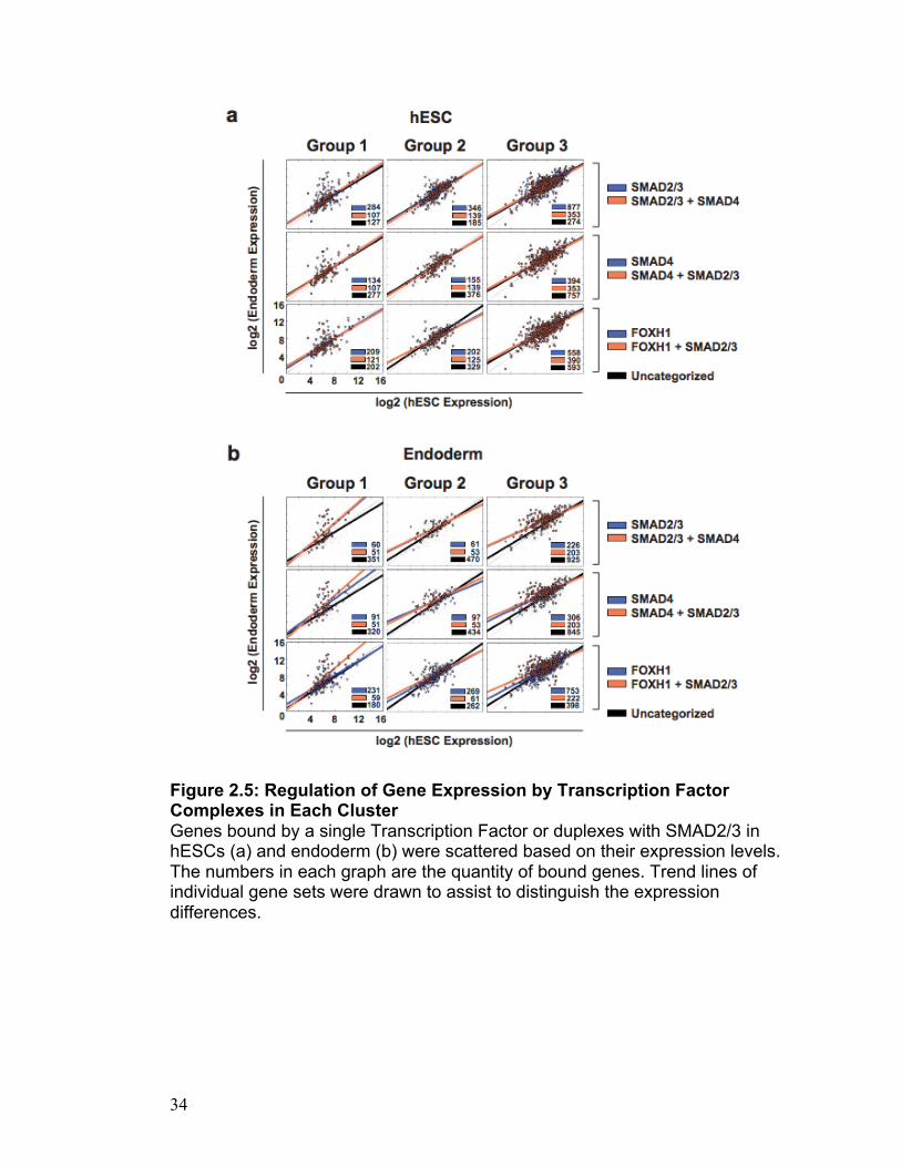
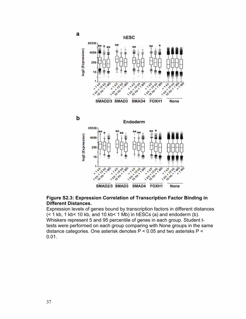
detectable binding. Surprisingly, we find that in both hESCs and derived

endoderm, the presence of a SMAD2/3, SMAD3, SMAD4 or FOXH1 binding

event within 1 kb of a TSS is significantly correlated with an increase in

transcriptional levels, above background levels (Student’s t-test; In hESCs, P

were 1.5E-50, 5.6E-38, 2.5E-15 and 5.6E-16, respectively; In endoderm, 3.5E-

12, 8.7E-12, 1.7E-05 and 4.3E-12, respectively; see Figure S2.2). Once this

distance is expanded to 10 kb or 1 Mb, this correlation diminishes for all

transcription factors.

We next examined only the 10 kb interval and asked whether the

accumulation of multiple SMAD2/3/4 or FOXH1 binding events could be

correlated with transcriptional activity. In derived endoderm, we find that three

or more binding regions of SMAD2/3, SMAD3, SMAD4 or FOXH1 proteins is

highly correlated with increased transcription levels and the more target

regions within this interval, the more significant the correlation. This correlation

is particularly strong for regions containing three or more SMAD2/3 or SMAD3

bound sites in derived endoderm (Student’s t-test; P = 1.5E-22 and 9.5E-16,

respectively; see Figure S2.4). Overall, this data strongly suggests that in both

hESCs and endodermal cells NODAL targets are more likely to be activated if

any of these transcription factors have concentrated regions of binding within

10 kb from the TSS.

19

Genome-Wide Mapping of Chromatin Marks, H3K4me3 and H3K27me3, in

hESCs and Derived Endoderm

As the regions surrounding the TSS appear to be critical for SMAD

activation of transcription, we next sought to examine whether these regions

are associated with particular chromatin conformations. To this end, we

performed ChIP-Seq using antibodies against H3K4me3 and H3K27me3. For

H3K4me3 and H3K27me3, we generated 7.3 and 17.9 million mapped reads

in hESCs and 10.3 and 19.6 million mapped reads in derived endoderm,

respectively (Table 2.1). Since the binding of H3K4me3 and H3K27me3 has a

far wider distribution than that of transcription factors, we sought to address

whether our depth of sequencing reached saturation. To this end, we called

peaks from pooled reads (two biological replicates for H3K4me3 and three for

H3K27me3) and checked the levels of saturation of unique peaks called.

H3K4me3 reads reached saturation, but not H3K27me3 even after additional

sequencing (Figure S2.5). To further verify these histone datasets, we

compared those generated for hESCs to other published accounts (Pan, Tian

et al. 2007; Zhao, Han et al. 2007). Although different hESC lines were used

(H9, H1, hES3), a high percentage of genes containing H3K4me3 peaks are

found in common (ours and Pan et al., 71% and 83%, respectively; ours and

Zhao et al., 68% and 88%, respectively). In contrast, relatively lower

percentage of genes containing H3K27me3 peaks are found in common (ours

and Pan et al., 64% and 50%, respectively; ours and Zhao et al., 44% and

65%, respectively). These data suggest that either more extensive sequence

20

depth might be necessary or that H3K27me3 marks are more variable than

H3K4me3 marks among cell lines.

Endoderm Contains Predominant Bivalent Domains

As it is known that bivalent domains containing both bound H3K4me3

and H3K27me3 become resolved during differentiation, we sought to examine

how these marks were altered during endoderm specification. To this end, we

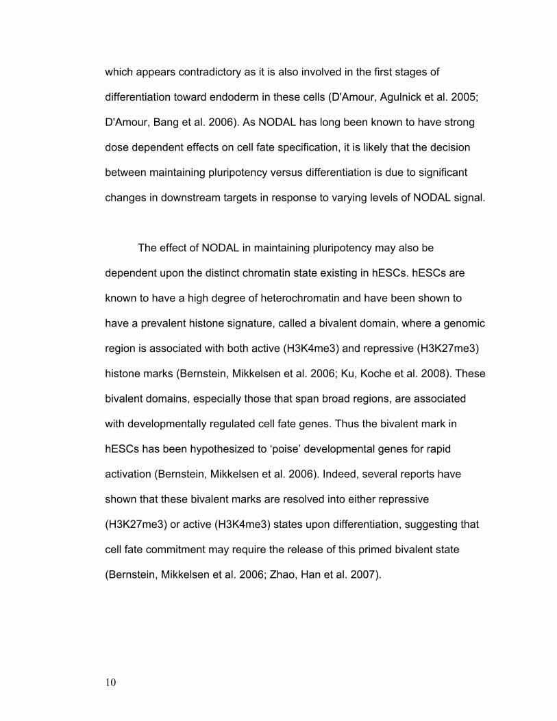
used K-means clustering to visualize H3K27me3 and H3K4me3 enrichment

around 16,621 TSSs in both hESCs and derived endoderm (Heintzman, Stuart

et al. 2007; Hon, Ren et al. 2008). This analysis enabled a clear demarcation

of nine different groups (1-9) containing unique signatures which exist in both

cell types (Figure 2.3). Furthermore, GO analysis defines these clusters,

showing that several have unique biological functions (Table S2.2).

Interestingly, in endoderm there are more bivalent classifications than in

hESCs as depicted by Groups 5-7. This is due to the addition of H3K27me3 in

narrow domains along these regions, which are not present in hESCs. The

bivalent groups with the strongest and widest H3K27me3 marks (Group 1 and

Group 4) are strongly associated with specific biological functions. Group 1

contains genes with roles in various developmental processes

("Developmental Group”; P = 1.1E-88). In this endodermal context however

this Group 1 ‘Developmental Group’ is highly enriched in regions involved in

endoderm formation, including EOMES, GSC, PITX2, SOX17 and GATA4.

Group 4 on the other hand contains genes with roles in cell adhesion and

21

communication (P = 2.5E-08 and 2.3E-14, respectively). While it is known that

the bivalent motif exists in various forms (Ku, Koche et al. 2008; Cui, Zang et

al. 2009), we were surprised to see how many different patterns emerged

upon clustering. Interestingly, unlike other more terminally differentiated cell

types, including neural precursor cells derived from embryonic stem cells,

endoderm appears to have maintained a high degree of bivalency(Bernstein,

Mikkelsen et al. 2006; Mikkelsen, Ku et al. 2007; Pan, Tian et al. 2007; Zhao,

Han et al. 2007).

As it is well known that different histone marks associate with activation

and repression of transcription, we were interested in understanding how

Groups 1-9 correlated with both SMAD binding and transcriptional activation in

the context of endoderm. To this end we used our microarray time course of

hESC differentiation into endoderm to associate the behavior of transcripts,

whether induced, constitutive, inactive, or repressed with a specific histone

grouping (1-9) (Figure S2.7a). Groups 3 and 6, which have predominant

H3K4me3 with minor H3K27me3, are associated with a range of

transcriptional behaviors, including induction, repression and constitutive

expression (both Groups 3 and 6; all P < 1.0E-03, see Experimental

Procedures for statistical analysis). Groups 8 and 9, which have little or no

H3K4me3 or H3K27me3, are associated - as might be expected - with inactive

regions (both P < 1.0E-03). Interestingly, Groups 1, 2 and 4 are associated

22

with transcripts that become activated upon differentiation (P < 1.0E-03, 1.5E-

02 and 2.8E-02, respectively).

SMAD2/3 Association Correlates with Resolution of Bivalent in Group 1.

While bivalent regions are prevalent in endoderm, we sought to

examine whether regions associated with active transcription were still in a

bivalent conformation in the endodermal cells. To this end, we examined only

transcripts that were induced during differentiation from hESCs to endoderm

and divided these into their bivalent groupings (1-9). Histogram plots of the

amount of H3K4me3 and H3K27me3 at each expressed region for each group

are shown in Figure 2.5. While the bivalent conformation is still observed, even

at expressed regions in most of the bivalent groups, this conformation is

strongly being resolved in Group 1 and moderately in Group 4 (Groups 1 and

4; all P for H3K4me3 and H3K27me3 < 1.0E-06, see Experimental Procedures

for statistical analysis.). Overall this suggests that Group 1 genes associated

with transcriptional activation upon differentiation toward endoderm have

unique chromatin alterations.

We next sought to determine whether SMAD2/3 binding could be

associated with these important chromatin changes. To this end, we examined

whether SMAD2/3 binding at the ‘induced’ regions could predict resolution of

bivalency. Of the 32 upregulated genes in Group 1, 21 genes were bound by

SMAD2/3. As illustrated in the browser shots of Figure 2.3 and Figure S2.5, all

23

21 of these regions displayed almost complete resolution of the bivalent

domain compared to much less resolution at the other loci (Figure 2.4b) (both

P for H3K4me3 and H3K27me3 < 1.0E-06). Interestingly, the 21 bound

regions included important endoderm specification genes, including EOMES,

GSC, SOX17, GATA4, GATA6, and FOXA2 (Table S2.3). This suggests that

SMAD2/3 directly or causally plays an important role in bivalent resolution

within these regions which are critical for endodermal specification and

provides a system in which to study how these key ‘poised’ regions become

activated.

Bivalent Domain is the Optimal Conformation for SMAD-Induced

Transcriptional Activation

The presence of SMAD2/3 is correlated with the resolution of bivalent

domains in Group 1, particularly at high expressed loci, including EOMES,

GSC, SOX17, GATA4, GATA6 and FOXA2, all endoderm specification

molecules. Here we sought to determine whether this SMAD2/3 association

was also predictive of active transcription. To this end, we analyzed the

location surrounding the TSS from each group for both SMAD binding and

resulting increase in transcriptional levels between hESCs and derived

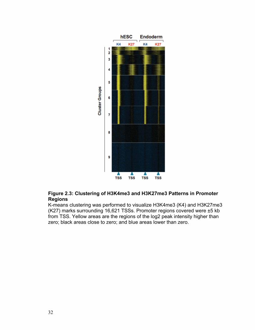
endoderm. Surprisingly, we find that the binding of SMAD2/3 within Group 1 is

predictive of expression changes only within the endoderm. This is illustrated

in Figure 2.6 where we plot the log2 value of hESC versus endoderm

expression on regions bound by SMAD2/3, SMAD4 and FOXH1. Only Group 1

24

genes show increased activation of transcription correlated with SMAD2/3

binding. This is further illustrated when using regions bound by combinations

of the transcription factors. Regardless of the combination of bound

transcription factors, the only transcription factor that can be associated with

transcriptional change is SMAD2/3 in the Group 1 context (Figure 2.5 and

Figure S2.8 and S2.9). These results strongly suggest that the endodermal

bivalent state with the broadest H3K4me3 and H3K27me3 domains is the

most conducive for activation of transcription by SMAD2/3. This activation is

mediated by SMAD2/3 binding, not SMAD4 or FOXH1 and is probably

precipitated by a resolving bivalent domain.

DISCUSSION

While many inroads have been made in understanding endoderm

formation in vertebrates, the next paradigm shifts in embryology will be

advanced by the application of new technologies. As ChIP-Seq becomes more

utilized in the scientific community, many reports have described transcription

factor binding in hESCs and other developmental cell types (Boyer, Lee et al.

2005). To date, our datasets are unique, representing not just a single

transcription factor, but a complex of factors. Furthermore, these datasets

follow the dynamics of this complex through developmental time – from

pluripotency to endoderm in hESCs. The generated datasets for SMAD2, 3, 4,

FOXH1, H3K4me3 and H3K27me3 provide insight into mechanisms

25

underlying how SMAD transcription factors mediate NODAL signaling to

specify endoderm.

During endoderm differentiation, SMAD transcription factors specify

target genes to be transcribed when they are required for the execution of the

NODAL-induced developmental program. The subsets of target genes

necessary for the closely related functions are likely to be coordinately marked

and expressed to meet the need. Although the means by which this

coordination of transcription factor-induced gene expression is achieved is not

clear, it is becoming apparent that chromatin modification plays a key role.

Recently, a number of studies have shown that the levels of histone

methylation and the recruitment of histone methyltransferase with transcription

factors are critical for their transcriptional activity (Demers, Chaturvedi et al.

2007; McKinnell, Ishibashi et al. 2008; Cheng, Wu et al. 2009). In agreement

with this view, we showed that chromatin conformation around the TSS plays

a critical role in deciding which groups of genes become activated by all

transcription factors studied. In this paper, we presented genomic evidence

that the surroundings of TSSs are specifically equipped with histone

methylation marks to fulfill this coordinated control. Interestingly, within the

endoderm, we have defined subtle classes of bivalent domains, each with

distinct annotations, transcriptional responses, and binding variability. Group 1

represents the bivalent domain whose function is to regulate ‘Developmental

Genes’ which recapitulates previous findings (Bernstein, Mikkelsen et al.

26

2006). In addition, we showed another subclass bivalent group, Group 4,

which is strongly annotated to neuronal activities and cell adhesion and is not

identified in other studies (Pan, Tian et al. 2007; Zhao, Han et al. 2007). While

a small fraction (less than 20%) of monovalent genes has been shown to

become bivalent in more differentiated cell types including mouse embryonic

fibroblasts (MEFs) and neural progenitor cells (NPCs) (Mikkelsen, Ku et al.

2007; Zhao, Han et al. 2007), we showed that most of the monovalent genes

with H3K4me3 appears to become bivalent during endoderm formation (as

observed in Groups 3, 5, 6, and 7). Since these various bivalent groups

revealed in derived endoderm are associated with distinct annotations and

display unique histone marks, they can be further classified into the types

associated with Polycomb repressive complexes (PRC) as previously

discussed (Ku, Koche et al. 2008). Groups 1 and 4 are likely to be PRC1-

positive because they exhibit large H3K27me3 regions and maintain the

bivalent conformation during differentiation as well as are strongly annotated

to development and cell signaling. Interestingly, Groups 5, 6 and 7 are likely to

contain PRC1-negative bivalent domains emerged during endoderm formation

as they display small H3K27me3 regions and are associated with non-

developmental functions such as protein and DNA metabolism. These groups

suggest that new genes may become poised throughout stages of

differentiation for new functions.

27

Overall, and unexpectedly, the bivalent domains in endoderm derived

from hESCs have not yet been resolved and even are increased from the

hESC state. This maintenance of bivalent state is distinctly different from what

has previously been reported. While bivalent domains are prevalent in hESCs,

encompassing more than 2000 promoters in the genome, most of these

bivalent domains are resolved in more differentiated cell types including MEFs

and NPCs (Bernstein et al., 2006; Mikkelsen et al., 2007; Pan et al., 2007;

Zhao et al., 2007). The resolution is particularly true for genes restricted to

regulation of specialized functions, strongly suggesting that the bivalent

resolves to monovalent to activate developmentally important gene

transcription. We suggest that the difference between the unresolved but

active endoderm bivalent domains, and the resolved bivalent domains in

MEFs and NPCs lies in the degree of differentiation. Endoderm is one of the

first cell types that arise in the embryo and therefore must maintain a degree

of plasticity. It might not be surprising that these more plastic cellular types

retain a more bivalent conformation and even may utilize new subtleties in this

conformation to activate gene transcription. Our observations at particular

endoderm-specific loci reflect an intermediate stage of the bivalent, not

completely resolved, but clearly changing toward a more monovalent state at

important promoter regions. In our case, this is reflected by the Group 1

promoters which are bound by SMAD2/3. These are highly active promoters in

hESC derived endoderm and include key endoderm specification genes,

including GATA4, GATA6, FOXA2, GSC, and PITX2. Interestingly, two thirds

28

of these promoters were bound by SMAD2/3 in hESCs, but were inactive in

that cell type and did not display the subtle H3K4me3 and H3K27me3

changes found within endoderm, possibly suggesting that SMAD binding

precedes the chromatin change. Whether this association is due to SMAD2/3

binding altering the conformation of the bivalents of this class or whether this

conformation allows for initial SMAD2/3 binding is unknown, but will be an

interesting avenue of further pursuit.

Accompanying this paper is the complete dataset for SMAD2/3,

SMAD3, SMAD4 and FOXH1 targets in hESCs and derived endoderm and

their effects on neighboring gene transcription, a resource that can be both

mined for enhancers of specific gene loci and for genomic studies. One of our

surprising findings is that SMAD2, 3, 4 binding is highly dynamic; few specific

target regions are maintained from hESCs to endoderm. This suggests that

the SMAD transcription complex is constantly in flux, using a variety of

different sites to elicit activation of individual loci. Furthermore, we also show

that FOXH1 has very different binding behavior than the SMAD proteins. First,

throughout differentiation, FOXH1 maintains association with the same

general genomic locations, whereas SMAD proteins become far more

localized in intergenic regions once cells have become endoderm. Second,

upon differentiation, FOXH1 exhibits widespread binding throughout the

genome whereas the SMADs become far more restricted to specific locales.

Third, FOXH1 binding has much less effect on transcriptional responses.

29

These all appear to be consistent with a role of FOXH1, not specifically as a

transcriptional activator, but as a pioneer protein which associates with

chromatin to recruit histone modifiers to these loci (Cirillo et al., 2002; Cirillo

and Zaret, 1999).

NODAL signaling is reused throughout development to guide the

formation of a plethora of tissue types. It has also been implicated in several

cancers (Xu, Zhong et al. 2004; Lee, Jan et al. 2010; Mangone, Walder et al.

2010). Despite the importance of this signaling pathway, few direct targets

have been elucidated since the SMAD transcription factors were identified

more than 14 years ago. Here we provide a comprehensive dataset that can

be used for the functional examination of thousands of additional targets.

These targets, several of which are bound by the SMAD complex in both

hESCs and derived endoderm, may also be bound and activated in a

multitude of other normal and diseased cell types. Thus, we anticipate that the

analysis of these factors will have wide-spread benefit to the scientific

community.

30

Figure 2.1: Cell Type-Specific Recruitment of SMADs and FOXH1 (a) Predicted genomic distribution of transcription factor binding. SMADs and FOXH1 targets were classified into annotated exons, introns, promoters, or intergenic region using UCSC Known Genes (Human browser hg18). Promoter regions are defined as regions within 10 kb from TSS. (b) Venn diagram representing the overlap of SMAD2/3 binding targets (upper left, Peaks) and associated genes (upper right, Genes) within 100 kb between hESCs (blue circle) and derived endoderm (red circle). The overlap of SMAD2/3 and FOXH1 binding targets (lower left) and SMAD2/3/4 targets (lower right) in derived endoderm.

31

Figure 2.2: Genome-Wide Mapping of SMAD2/3, SMAD4, H3K4me3 and H3K27me3 Using ChIP-Seq UCSC genome browser screen shots showing the loci of SMAD2/3 and SMAD4 binding and histone marks in the genome of EOMES and GSC in hESCs (blue) and derived endoderm (red). Dotted boxes indicate unique regions of SMAD2/3 and SMAD4 binding in derived endoderm, and asterisk indicates ACTIVIN response element in the promoter region (Danilov et al., 1998). K4 and K27 stand for H3K4me3 and H3K27me3, respectively.

32

Figure 2.3: Clustering of H3K4me3 and H3K27me3 Patterns in Promoter Regions K-means clustering was performed to visualize H3K4me3 (K4) and H3K27me3 (K27) marks surrounding 16,621 TSSs. Promoter regions covered were ±5 kb from TSS. Yellow areas are the regions of the log2 peak intensity higher than zero; black areas close to zero; and blue areas lower than zero.

33

Figure 2.4: Chromatin Signature Changes in Differentially Expressed and SMAD2/3 Bound Genes (a) The peak levels (histograms) of H3K4me3 (K4) and H3K27me3 (K27) in both hESCs and endoderm. Black solid lines indicate the histograms of all genes in each Group. Induced genes are represented in red lines. R represents normalized enrichment over the background. (b) The histograms of H3K4me3 (K4) and H3K27me3 (K27) peaks of Group 1 genes induced and also bound by SMAD2/3 in endoderm. SMAD2/3 bound and not-bound genes were represented in red and blue lines, respectively.

34

Figure 2.5: Regulation of Gene Expression by Transcription Factor Complexes in Each Cluster Genes bound by a single Transcription Factor or duplexes with SMAD2/3 in hESCs (a) and endoderm (b) were scattered based on their expression levels. The numbers in each graph are the quantity of bound genes. Trend lines of individual gene sets were drawn to assist to distinguish the expression differences.

35

Figure S2.1: ChIP Assay for SMAD2/3/4 and FOXH1 Binding to Known Targets H9 hESCs were differentiated to definitive endoderm by ACTIVIN treatment for 5 days. Cells were harvested and processed for ChIP with anti-SMAD2/3, SMAD3, SMAD4, or FOXH1 antibodies. The fold enrichment of the precipitated DNA by each of the antibodies versus the input control was determined by qPCR using positive target primers for LEFTY1 and LEFTY2 and negative target primer for GAPDH intronic region.

36

Figure S2.2: SMAD/FOXH1 Targets in hESCs and Derived Endoderm within 1 Mb, 10 kb and 1 kb from TSS. (a) Venn diagram representing the overlapping targets of SMAD2/3 between hESCs (blue circle) and derived endoderm (red circle). (b) Overlapping targets of SMAD2/3 (red circle) and FOXH1 (blue circle) in derived endoderm. (c) Overlapping targets of SMAD2/3 (red), SMAD3 (purple) and SMAD4 (green) in derived endoderm.

37

Figure S2.3: Expression Correlation of Transcription Factor Binding in Different Distances. Expression levels of genes bound by transcription factors in different distances (< 1 kb, 1 kb< 10 kb, and 10 kb< 1 Mb) in hESCs (a) and endoderm (b). Whiskers represent 5 and 95 percentile of genes in each group. Student t-tests were performed on each group comparing with None groups in the same distance categories. One asterisk denotes P < 0.05 and two asterisks P < 0.01.

38

Figure S2.4: Expression Correlation of Transcription Factor Binding with Different Sites. Expression levels of genes with different numbers of transcription factor binding sites in hESCs (a) and endoderm (b). Genes bound by transcription factors within 10 kb were analyzed. Whiskers represent 5 and 95 percentile of genes in each group. Student t-tests were performed on each group comparing with the None group < 10 kb. One asterisk denotes P < 0.05 and two asterisks P < 0.01.

39

Figure S2.5: H3K4me3 and H3K27me3 ChIP-Seq Peak Saturation. Peaks were called from each bin of the pooled reads and the numbers of unique peaks called were plotted to check the levels of saturation (see Experimental Procedures).

40

Figure S2.6: Genome-Wide Mapping of SMAD2/3, SMAD4, H3K4me3 and H3K27me3 UCSC genome browser screen shots showing the loci of SMAD2/3 and SMAD4 binding and histone marks in the genome of FOXA2, ACSS1 and LMO1 in hESCs (blue) and derived endoderm (red). FOXA2 is an induced Group 1 gene, and ACSS1 and LMO1 are Group1 genes but not in the induced subset. K4 and K27 stand for H3K4me3 and H3K27me3, respectively.

41

Figure S2.7: Enrichment of Differential Gene Expression and Transcription Factor Binding in Clusters. (a) The numbers of genes observed in each expression categories (induced, repressed, constitutive and inactive during hESC differentiation to endoderm) were plotted in red bars. The numbers of genes in random occurrence (average of 1000 random pulls) were plotted in blue bars. (b) The numbers of genes bound by SMAD2/3, SMAD4 or FOXH1 were plotted in red bars. The numbers of genes in random occurrence (average of 1000 random pulls) were plotted in blue bars. Upper panel: genes bound in hESCs, Lower panel: newly bound genes in endoderm.

42

Figure S2.8: Regulation of Gene Expression by Transcription Factor Complexes in Clusters. Genes bound by a single Transcription Factor or duplexes with either SMAD4 or FOXH1 in hESCs (a) and endoderm (b) were scattered based on their expression levels. The numbers in each graph are the quantity of bound genes. Trend lines of individual gene sets were drawn to assist to distinguish the expression differences.

43

Figure S2.9: Regulation of Gene Expression by Triple Transcription Factor Complexes in Clusters. Genes bound by a single Transcription Factor or triplexes in hESCs (a) and endoderm (b) were scattered based on their expression levels. The numbers in each graph are the quantity of bound genes. Trend lines of individual gene sets were drawn to assist to distinguish the expression differences.

44

Table 2.1: ChIP-Seq Data and Analysis Summary The numbers of reads, peaks and associated genes of all transcription factors and histone marks studied are presented separately in hESCs and derived endoderm (Endo).

Table 2.1: ChIP-Seq Data and Analysis Summary

Associated Genes (kb) ChIP Cell Reads Peaks

1000 100 10 1

hESC 10,200,000 4,032 3,588 3,077 1,916 1,249 SMAD2/3_A

Endo 9,605,287 1,037 1,117 827 272 72

hESC 8,708,351 14,833 9,777 9,052 7,057 5,715 SMAD2/3_B

Endo 5,910,789 2,915 2,604 1,905 567 106

hESC 6,928,056 2,688 2,511 2,062 1,197 745 SMAD3

Endo 6,055,629 2,296 2,107 1,466 400 67

hESC 8,959,821 3,936 3,533 3,223 2,293 1,702 SMAD4

Endo 6,066,743 4,531 2,768 2,753 906 207

hESC 10,400,000 9,702 6,897 5,797 2,646 1,123 FOXH1

Endo 10,800,000 29,292 11,631 10,385 4,734 1,324

hESC 9,465,441 - - - - Input

Endo 9,716,862 - - - -

hESC 7,338,695 24,030 H3K4me3

Endo 10,326,110 29,688

hESC 17,893,702 13,936 H3K27me3

Endo 19,595,165 26,293

hESC 8,824,050 - Input

Endo 10,876,757 -

45

Supplemental Table S2.1: Expression of Lineage Specification Genes

Gene Day 0 Day 1 Day 3 Day 5

GSC 73 29 31 24 1424 3320 1248 1614 2829 2806 2967 2985

EOMES 180 95 78 158 4488 7220 4228 3589 3696 4228 4820 4957

MIXL1 252 186 159 141 4188 10592 4883 2653 5151 5767 7088 6971

Table S2.1: Expression of Lineage Specification Genes Individual numbers in each gene and time point represent expression data from biological replicates.

46

Supplemental Table S2.2: Gene Ontology Analysis of Cluster Groups Biological Process p-value

Group 1 mRNA transcription regulation 6.91E-93 Developmental processes 1.11E-88 mRNA transcription 1.47E-86 Ectoderm development 1.50E-66 Neurogenesis 1.18E-63 Nucleoside, nucleotide and nucleic acid metabolism 1.09E-58 Segment specification 1.08E-27 Mesoderm development 1.51E-20 Embryogenesis 3.75E-16 Other receptor mediated signaling pathway 3.85E-12 Anterior/posterior patterning 4.18E-12 Skeletal development 2.35E-11 Cell communication 9.68E-09 Oncogenesis 2.42E-06 Muscle development 6.34E-05 Cell proliferation and differentiation 8.22E-05

Group 2 mRNA transcription 2.30E-07 Nucleoside, nucleotide and nucleic acid metabolism 3.58E-07

Group 3 Nucleoside, nucleotide and nucleic acid metabolism 2.17E-11 mRNA transcription 9.57E-10 mRNA transcription regulation 5.41E-09 Oncogenesis 9.36E-08 Developmental processes 2.72E-06 Protein phosphorylation 1.65E-05

Group 4 Neuronal activities 7.48E-24 Signal transduction 1.35E-21 Ion transport 1.63E-15 Cell communication 2.27E-14 Synaptic transmission 3.97E-13 Cation transport 1.30E-12 Transport 3.35E-12 Cell adhesion 2.49E-08 Cell surface receptor mediated signal transduction 4.79E-06 Cell adhesion-mediated signaling 4.63E-05

Group 5 Intracellular protein traffic 9.22E-08 Protein metabolism and modification 1.01E-06

Group 6 (Protein metabolism and modification) (1.30E-03) Group 7 (DNA metabolism) (1.62E-02) Group 8 Immunity and defense 3.15E-18

Cell surface receptor mediated signal transduction 2.63E-08 Signal transduction 8.76E-07 Cytokine and chemokine mediated signaling pathway 1.21E-06 Cell structure 7.30E-06 Cell structure and motility 8.27E-06 Muscle contraction 2.72E-05

Group 9 Olfaction 5.98E-54 Chemosensory perception 5.00E-53 Sensory perception 2.52E-42 G-protein mediated signaling 3.03E-32 Cell surface receptor mediated signal transduction 2.10E-21 Immunity and defense 1.03E-11 Signal transduction 3.69E-08 Interferon-mediated immunity 1.51E-07

47

Cytokine and chemokine mediated signaling pathway 4.11E-06 Table S2.2: Gene Ontology Analysis of Cluster Groups GO terms in the biological process with P below 1.0E-05 are listed in each Group.

48

Supplemental Table S2.3: Induced Genes in Group 1

Gene Accession No. hESC Expression

Endoderm Expression

SMAD2/3 Target

NTF3 NM_001102654 23 97 * PITX2 NM_000325 401 1617 * EOMES NM_005442 104 3052 * MXI1 NM_130439 228 628 * DUSP4 NM_001394 188 1028 * FOXA2 NM_021784 121 859 * GATA4 NM_002052 62 1238 * PLXNA4 NM_020911 121 306 * NTN1 NM_004822 35 416 * TBX3 NM_016569 29 184 * C1orf61 NM_006365 69 500 * EPHB3 NM_004443 81 325 * HLX NM_021958 52 189 * PDE10A NM_006661 85 564 * FOXQ1 NM_033260 71 884 * SFRP1 NM_003012 1253 3359 * FGF17 NM_003867 97 5132 * GSC NM_173849 45 2058 * HAND1 NM_004821 36 154 * GATA6 NM_005257 118 4761 * SOX17 NM_022454 80 1869 * NOG NM_005450 44 360 - TPPP3 NM_015964 41 197 - PCDH7 NM_032457 171 546 - HNF1B NM_000458 40 245 - CYP26A1 NM_000783 1191 6523 - COL2A1 NM_001844 69 374 - AHNAK NM_001620 406 1274 - SHH NM_000193 92 287 - DLX5 NM_005221 37 241 - CRLF1 NM_004750 2237 3251 - MSX2 NM_002449 65 640 -

Table S3. Induced Genes in Group 1 SMAD2/3 targets are marked by an asterisk.

49

EXPERIMENTAL PROCEDURES Cell Culture and Differentiation

Undifferentiated H9 hESCs (WiCell) were maintained on mouse

embryonic fibroblast (MEF) feeder layers or on Matrigel (1:20 dilution; BD

Biosciences) in mouse embryonic fibroblast-conditioned medium (CM). CM

was produced by conditioning MEFs for at least 24 hours in Dulbecco's

modified Eagle's medium/Ham's F-12 medium (DMEM/F12) supplemented

with 20% knockout serum replacement (Gibco), 1 mM L-glutamine, 0.1 mM

nonessential amino acids, 0.1 mM 2-mercaptoethanol, and 8 ng/ml

recombinant human fibroblast growth factor-basic (bFGF; Peprotech). Cultures

were routinely passaged with 200 U/ml type IV collagenase (Gibco) at the split

ratio of 1:3 to 1:4 every 4–5 days.

Definitive endoderm precursors were generated from hESCs as

previously described (D'Amour et al., 2005). Differentiation was performed in

RPMI-1640 medium supplemented with glutamax, 100 ng/ml recombinant

human ACTIVIN A (R&D Systems), penicillin/streptomycin, and defined fetal

bovine serum (FBS; HyClone) at the sequentially increased concentrations (0,

0.2 to 2%). 2% FBS was maintained afterwards in cultures over the duration of

differentiation.

Endoderm formation was validated by real-time RT-PCR with the total

RNAs isolated from differentiated cells. After washing once in phosphate

buffered saline pH 7.4 (PBS) containing 0.2% bovine serum albumin (BSA),

cells were harvested in Trizol (Invitrogen) and total RNAs were isolated

according to the manufacturer's protocol. One-step RT-PCR was performed

on iCycler (BioRad) using iScript RT-PCR SYBR Green Supermix (Bio-Rad).

The primer sequences are previously described (D'Amour et al., 2005).

50

Gene Expression Time course gene expression was performed on day 0, 1, 3, and 5

differentiated cells. Cells were washed once in PBS containing 0.2% BSA and

used for total RNA preparation using Trizol (Invitrogen). rRNAs were removed

from the isolated total RNAs and gene expression was analyzed using

GeneChip Human Exon 1.0 ST Array (Affymetrix) at the Stanford shared

protein and nucleic acid (PAN) facility. Exon array data were processed using

GeneBASE (Kapur et al., 2007). Probe intensities were corrected using

background probes. Probes were selected and summarized for gene level

expression. Gene expression profiles were pooled for quantile-normalization.

To examine gene expression specific to endodermal cells, CXCR4

positive cells were isolated from day 5 differentiated cells using FACS. Cells

were harvested and dissociated using 0.05% trypsin/EDTA (Invitrogen)

followed by neutralization with PBS containing 10% FBS. Cells were strained

with 40 µm strainer (BD Biosciences) and washed twice in PBS containing

0.2% BSA and 0.09% sodium azide (Staining Buffer). Cells were labeled with

antibodies against CXCR4-Phycoerythrin (R&D Systems) at 10 µl per 2.5x105

cells for 30-45 minutes on ice. Cells were washed twice and resuspended in

the Staining Buffer. CXCR4 positive cells were analyzed and isolated using a

FACS Aria (BD Bioscience) at the Stanford shared FACS facility. Isolated cells

were either used for total RNA preparation using Trizol (Invitrogen) or cross-

linked with formaldehyde for chromatin immunoprecipitation (ChIP).

ChIP-Seq ChIP was performed as previously described (Johnson et al., 2007).

5x106 cells cross-linked with formaldehyde were used for each ChIP. The

cross-linked cells were sonicated in 500 µl of a lysis buffer (50 mM Tris pH8.1,

10 mM EDTA, 1 % SDS) with protease inhibitor cocktail (Roche) to generate

200- to 600-bp fragments. Fragmented chromatin was immunoprecipitated

with magnetic beads coupled with 5 µg of each antibody. The antibodies used

51

were anti-SMADd2/3 (Santa Cruz Biotechnology, sc-8332 or R&D Systems,

AF3797), anti-SMAD3 (Abcam, ab28379), anti-SMAD4 (R&D Systems,

AF2097), anti-FOXH1 (R&D Systems, AF4248), anti-H3K4me3 (Abcam,

ab8580) and anti-H3K27me3 antibody (Upstate, 07-449). After washing,

precipitated DNA was purified and an aliquot was used for PCR validation.

The primers used for qPCR to quantify the ChIP-enriched DNA are as

follows: For transcription factor ChIP, LEFTY1(Forward, 5’-

TGTTTGCAGAGGGATAATAG-3’; Reverse, 5’-

TAATTCACAGGACTGATTGG-3’), LEFTY2 (Forward, 5’-

AGCCTGAAGAGTTTTGTTTG-3’; Reverse, 5’-TCCTGACGACTAA

TCAGACC-3’), GAPDH (Forward, 5’-AAGTGGATATTGTTGCCATC-3’;

Reverse, 5’-GGAATACGTGAGGGTATGAA-3’), and negative control

(Forward, 5’-TAGCCAAAAG AAGGAAGCAACAG-3’; Reverse, 5’-

CTAAAGGTAG GGCTGGAAGCAAT-3’). For histone ChIP, GAPDH (Forward,

5’-TCGACAGTCAGCCGCATCT-3’; Reverse, 5’-

CTAGCCTCCCGGGTTTCTCT-3’), RLP30 (Forward, 5’-

CAAGGCAAAGCGAAATTGGT-3’; Reverse, 5’-

GCCCGTTCAGTCTCTTCGATT-3’), MYOD (Forward, 5’-

CCGCCTGAGCAAAGTAAATGA-3’; Reverse, 5’-GGCAACCGCTGGTTTGG-

3’), and SERPINA1 (Forward, 5’-GGCTCAAGCTGGCATTCCTG-3’; Reverse,

5’-GGCTTAATCACGCACTGAGCTTA-3’). Relative occupancy values were

calculated by determining the apparent immunoprecipitation efficiency (ratio of

the amount of immunoprecipitated DNA to that of the input sample) and

normalized to the level observed at a negative control region, which was

defined as 1.0.

Sequencing libraries were prepared using Genomic DNA Sample Kit

(Illumina) according to the manufacturer's protocol. The ChIP-Seq libraries

were sequenced by Genome Analyzer II (Illumina) and its analyzing program.

52

Sequencing Data Processing Transcription factor ChIP-Seq reads were processed to call peaks using

CisGenome, an analyzing tool for genomic data (Ji et al., 2008). The setting

for calling and sliding window size was 300 bp and the threshold number of

reads required for peak to be called was 11 reads. The false discovery rate

allowed was 0.01. The resulting peaks were mapped to the human genome

hg18 to identify the locations and numbers of peaks around annotated genes.

Histone H3K4me3 and H3K27me3 peaks were called using QuEST 2.4

(Valouev et al., 2008). We used the “histone” bandwidth setting with “relaxed”

peak-calling parameters.

Transcription Factor Binding Regions and Associated Genes

We parsed the targets to see their distributions across the gene body.

UCSC Known Genes (Human browser hg18) were used to locate the targets

into annotated genomic regions, exon, intron, promoter (±10 kb from TSS), or

intergenic region. The numbers of the target peaks reaching at least 1 bp into

each genomic region were counted. To avoid multiple counting due to

overlapping two different regions, the regions of target binding were

sequentially searched in the order of promoter, exon, intron, and intergenic

region. In addition, when we analyzed the numbers of overlapping targets

existing for each transcription factor between the two cell states, the numbers

of the target peaks which are remained at least 1 bp from the previous site

were counted.

We examined the overlap between genes called within the regions

bound by all of the transcription factors analyzed. For the associated genes for

each target, the nearest genes within 1 Mb, 100 kb, 10 kb and 1 kb from TSS

were counted. Further, we examined the numbers of genes lying within target

53

regions between hESCs and endoderm within the same distance categories

(Figure 1B and Figure S2).

Using the expression timecourse, we determined the most favorable

context of SMAD2/3/4 or FOXH1 binding that could be correlated to a

transcriptional response. First, we examined all regions in the genome

surrounding a TSS at 1 kb, 10 kb and 1 Mb and analyzed the expression

levels of genes identified to contain regions bound to SMAD2/3/4 or FOXH1.

Second, we examined all genomic regions surrounding a TSS at 10 kb with

different numbers (one, two, or more than three) of SMAD2/3/4 or

FOXH1bound site. Student’s t-tests were performed to determine correlation

of those transcription factor bindings with transcription levels.

Histone Modification and Associated Genes To determine sequence library saturation, we simulated random

subsets for each library. We examined how many more peaks were

computationally identified using 10% of all reads, up to 100% in 10%

increments. In this way, if significantly more peaks are called when using

100% of reads versus 90%, then the library is not yet saturated. If the number

of identified peaks levels off with <100% of reads, then the library is

considered saturated.

To further verify our H3K27me3 and H3K4me3 ChIP-Seq datasets, we

compared the datasets generated for hESCs to other published accounts (Pan

et al., 2007; Zhao et al., 2007). Specifically, we identified the number of genes

in the intersection of the set of genes that were within 10 kb of reads in our

dataset, and another set of genes that were within 10 kb of reads in other

published work.

Histone Peak Clustering We used K-means clustering (http://bonsai.ims.u-

tokyo.ac.jp/~mdehoon/software/cluster/software.htm) to visualize the

54

H3K4me3 and H3K27me3 surrounding TSS in the genome. The

wiggle/enrichment plots represent normalized enrichment over the

background. The data points were the normalized enrichment values that are

calculated by QuEST. The log2(enrichment) values were used for clustering

and plotting. H3K4me3 and H3K27me3 marks were analyzed depending on

their patterns within ±5 kb of the TSS from UCSC Known Genes. For gene loci

with isoforms with alternate TSS's, we chose the TSS with the largest

H3K4me3 peak. Genes with a TSS within 10 kb of another gene TSS were

discarded for clustering analysis.

To functionally define these clusters, GO analysis was performed using

DAVID (the Database for Annotation, Visualization and Integrated Discovery)

(http://david.niaid.nih.gov). In addition, we examined how Groups 1-9 are

correlated with transcriptional activation in the context of endoderm. To this

end we used our microarray timecourse of hESC differentiation into endoderm

to associate the behavior of transcripts, whether induced, constitutive, inactive,

or repressed with a specific histone grouping (1-9). We compared the day 5

CXCR4 positive samples (d5) with hESC samples (d0). For each gene, we

calculated the fold change (R), difference (D) between the means of the two

groups, and the Welch's t-test p-value using dChip (Li and Wong, 2001).

Induced genes were defined by R > 2 and D > 100 of d5 over d0, and P ≤

0.05. Repressed genes were defined by R > 2 and D > 100 of d0 over d5, and

P value <=0.05. We also calculated the logarithm-transformed average (A)

and difference (M) of the means of d0 and d5 for each gene. We calculated

the z-scores of A (ZA) and the z-scores of M (ZM) for all genes. Constitutive

genes were defined by ZA > 1 and ZM < 1. Inactive genes were defined by ZA <

-1 and ZM < 1.

Transcription Factor Binding and Histone Marks We compared genes bound by the transcription factors to each histone

group to examine whether different groups are enriched for genes associated

55

with SMAD2/3, SMAD4 or FOXH1. We counted the genes bound by

SMAD2/3, SMAD4 or FOXH1 within 100 kb (until reaching other gene) in each

histone group. These counts were compared with the numbers of genes in

random occurrence in each group. For each cluster group with N genes, we

calculated a background expectation by randomly drawing N genes from the

total sample and recording the number, repeated 1000 times. In addition, we

examined whether the binding of transcription factors within each group is

predictive of expression changes between hESCs and derived endoderm. We

analyzed the location within 100 kb (until reaching other gene) surrounding the

TSS from each group for both factor binding and resulting increase in

transcriptional levels. Further, we also compared the regions bound by

combinations of the transcription factors in each group. We identified

complexes by using a sliding window of 600 bp. Student’s t-tests were

performed to elucidate correlation of those transcription factor bindings with

transcription levels.

We examined whether there is a subsignature within histone groups

that is conformationally distinct for transcription factor binding and

transcriptional increase. To this end, we analyzed the extent of H3K4me3 and

H3K27me3 association around TSS regions of subgroups bound by

transcription factors and compared with those that are not related with

transcription factor binding. The changes of H3K4me3 and H3K27me3 peaks

were statistically analyzed as follows: within each cluster group, we calculated

the average profile for all the genes in the whole group (across 100 bins). We

took the subset of interest (e.g. genes bound by SMAD2/3 in endoderm) and

calculated the average profile for that. Then we calculated the sum of squares

of the deviation from the mean at each bin to get a measure of deviation from

the whole group. We permuted 1000 random groups of the same size as the

original subset and calculated the background distribution of scores.

56

CHAPTER 3

ChIPvect_gui: Cell Specific Vector Generated Surface Plots

Invention Disclosure Docket Number: 08-330 Stanford University Office of Technology Licensing

57

ABSTRACT

Chip-seq has enabled scientists to paint an accurate picture of genetic

occupancy by identifying regions in the genome that are occupied by

transcription factors and/or modified histone proteins of interest with a high

degree of accuracy (Johnson, Mortazavi et al. 2007). This new technology has

spawned an array of bioinformatics tools that are designed to organize and

prime these data for analysis and the extraction of meaningful conclusions

(Valouev, Johnson et al. 2008). Though the bioinformatics tools currently

available are extremely useful in their own right, the need for an intuitive

method that capitalizes on chip-seq data to decipher the unique identity of a

given cell type remains apparent. The software invention presented here -

ChIPvect_gui - has been created using MATLAB as a platform, and it aims to

meet this need in a way that will be understandable and accessible to any

scientist that possesses a basic level of competence using a personal

computer.

58

BACKGROUND

Coupling chromatin immunoprecipitation with high-throughput sequencing has

yielded a technique that provides an accurate account of the regions in the

genome that are bound by certain transcription factors or associated with

histone proteins that are modified in a specific way (Bernstein, Mikkelsen et al.

2006; Johnson, Mortazavi et al. 2007). In turn, identifying gene regions that

are bound by certain transcription factors may hint at the role of genes during

development and cellular differentiation (Visel, Blow et al. 2008). It is

imperative that data of this quality and importance be presented in ways that

will highlight the striking epigenetic patterns that are inherent within it.

ChIPvect_gui is designed to illuminate striking histone modification and

transcription factor binding patterns that are present in chip-seq data.

ChIPvect_gui is based on fundamental concepts from linear algebra theory

and is built with a user-friendly graphical user interface (GUI) that makes the

package easy for any scientist with a basic level of competency using a

personal computer to understand. The software package has a variety of tools

and features that expose the user to novel ways of visualizing chip-seq data.

Each feature of ChIPvect_gui can be accessed through a simple click of the

appropriate button in the GUI at the appropriate time. To use ChIPvect_gui, an

input text file in tab-delimited (.txt) format, containing the relevant data is

59

required. Such files may be generated by the user in Microsoft excel or any

other text editor software package such as Text Wrangler.

Here, each feature of ChIPvect_gui is presented in detail. The concept behind

each one of the features in carefully described, and the functionality of each

feature is demonstrated using an example dataset. The MATLAB code written

to generate the GUI is also included in this chapter.

60

RESULTS

Application Features: Surface Plot

To use this feature of ChIPvect_gui, the user must provide data from three

separate chip-seq experiments performed on the same cell type. Each chip-

seq experiment is to be performed using an antibody that binds specifically to

a unique protein of interest. The surface plot function acts to generate a 3D

surface based on an input data file containing data from the three separate

chip-seq experiments referred to above. This input data matrix is n rows by 3

columns in size as illustrated in Table 3.1. Each column of the input data

matrix represents the number of sequence tags discovered in each of the

three chip-seq experiments. Each row of the input data matrix contains

specific genes that the user is interested in examining. Therefore, the entry in

the nth row of the mth column of the matrix contains the number of sequence

tags found to be associated with the nth gene in the mth chip-seq experiment.

Upon receipt of this input data matrix, the surface plot functionality of

ChIPvect_gui creates the three-dimensional surface in the following way. An

input data matrix in the same form as that seen in Table 3.1 is laid flat on the

X-Y plane in three-dimensional space, and a dot is placed above the X-Y

plane in the middle of each cell within the matrix. The unique thing about the

dots is that they rise to a height above the X-Y plane that is tantamount to the

number within each respective box. For example, if a certain gene in an

experiment had a total of 1000 sequence tags associated with it, the surface

61

plot feature would generate a dot rising 1000 units above the X-Y plane in the

middle of the appropriate cell of the corresponding matrix. This same

procedure is repeated for all the data points in the matrix leading to an array of

dots at varying heights and positions in three-dimensional space. Next, all

such dots are connected resulting in a three-dimensional surface that is

representative of the unique epigenetic patterns present in a distinct cell type.

Figure 3.1 depicts one such surface.

Application Features: Vector Plot & Vector Plot Annotation

The vector plot feature of ChIPvect_gui utilizes a matrix that is identical to that

accepted by the surface plot functionality shown in Table 3.1. The output

however, is markedly different. In this case, chip-seq data is presented in a

three-dimensional vector field. Each vector in the three-dimensional vector

field represents one gene, and the numerical contents of each row represent

the X, Y, and Z components of each vector. For example the 3D vector

representing Nanog in Table 3.1 would have 0.255056, 0.955676, and

0.827119 as its X, Y, and Z components respectively. A vector for each gene

in the list provided by the user is created in the same way. Figure 3.2 depicts

an array of vectors generated from the data set in Table 3.1. This data comes

from a chip-seq experiment in which the genetic occupancy of Oct4, Sox2, and

Nanog were examined in mouse embryonic stem cells (mESC) (Chen, Xu et

al. 2008).

62

To complement the vector plot functionality of ChIPvect_gui, a vector plot

annotation feature has also been added. This feature takes the form of a

checkbox in the gui. When selected, it simply labels each vector in three-

dimensional space with the appropriate gene name. This is designed to give

the user a better sense of the vector that represents each gene, and indirectly

allows the user to gauge the relative magnitude of occupancy of each

transcription factor on each gene.

Application Features: Vector-Generated Surface

The vector-generated surface is an important extension of the vector plot. The

vector plot serves as a skeletal framework for the vector generated surface/

The vector-generated surface is created by connecting the tips of all the

vectors in the vector plot to form a three dimensional shape that can be used

to identify a specific cell type. One such shape is depicted in Figure 3.3 and it

is uniquely defined by the pattern of transcription factor occupancy associated

with user-selected genes. The vector-generated surface could serve as a

readily available visual aid for the classification of cell types.

63

Application Features: Chromposition Chromposition provides yet another intuitive way of creating a three-

dimensional shape from ChIP-seq data. In contrast to the surface plot and

vector plot features, chromposition takes the location of each discovered

sequence tag into consideration when producing the three-dimensional shape.

It is important to note that the form of the matrix accepted by this feature of the

chipvect_gui software package is quite different from the matrices accepted by

the first three features described above. A truncated form of the matrix

accepted by this feature is depicted in Table 3.2. This data is obtained from

efforts to map STAT1 targets in interferon-γ stimulated HELA cells (Robertson,

Hirst et al. 2007).

Upon receipt of the input data matrix, chromposition generates a

representative three-dimensional shape in the following way. First,

chromposition generates a virtual circle drawn with 22 lines that are evenly

spaced apart from one another and run from the center of the circle to its

circumference. Each line represents one of the 22 chromosome pairs in the

human genome and is labeled accordingly (i.e. “Chr1” through “Chr22”). For

each distinct row in the matrix shown in Table 3.2, this feature of chipvect_gui

“looks” in the first column for the chromosome number and tags the

appropriate line that represents the current chromosome. It then takes the

number in the second column which is the position on the chromosome where

a majority of the tags were found and locates the exact point on the relevant

64

virtual chromosome to which it corresponds. A dot is placed directly above the

located point on the chromosome, at a height that is tantamount to the number

of tags associated with the data point in question. This procedure is repeated

for each row generating a large amount of data points in three-dimensional

space. Finally, connecting all the dots that have been generated from the

matrix containing the data of interest generates a 3D shape. Figures 3.4 and

3.5 provide a pictorial representation of the ideas discussed above.

Application Features: Custom Data Cursor The chromposition feature of chipvect_gui has been fitted with a custom data

cursor that displays the chromosome number and the amount of sequence

tags associated with a given peak. This feature was designed to make it easy

for any user to quickly and accurately determine the basic information

associated with a given data peak. Usage of the custom data cursor is

illustrated in Figure 3.5, where the chromosome number, number of tags, and

position on the chromosome associated with a specific peak displayed.

65

DISCUSSION

Chip-seq has emerged as a potent method for determining the patterns of

transcription factor occupancy and histone modification within cell groups of all

kinds (Bernstein, Mikkelsen et al. 2006; Johnson, Mortazavi et al. 2007; Chen,

Xu et al. 2008). It provides a more in-depth data set than its predecessor -

chip-chip - as scientists can now directly gauge transcription factor binding in

the genome rather than rely on oligomer hybridization to pre-made probes for

the detection of transcription factor occupancy. This advance in the field of

genomics has inspired the development of many potent computational tools

directed at priming data for the discovery of unique patterns (Ji, Jiang et al.

2008; Valouev, Johnson et al. 2008). With data of this quality readily available,

the need for computational techniques that build upon current methods to

highlight unique transcription factor binding patterns has become increasingly

apparent. Here we report the creation of a software tool that can be used to

present chip-seq data in novel ways, which serve to highlight interesting trends

contained within it.

Current computational tools that are used for chip-seq data analysis can be

used to convert the raw data to sequence tag form, which can then be readily

aligned with the genome of the appropriate model organism (Valouev,

Johnson et al. 2008). While this is very important for chip-seq data analysis,

there are a few analytical vantage points that are missing from this approach.

66

First, this method of presenting chip-seq data does not afford the user an

opportunity to examine the entire dataset at a glance. Second, the user is not

presented with the opportunity to ascertain if there is a unique binding pattern

for the transcription factor(s) under inspection that characterizes each cell

type. And lastly, it is rare to find a computational tool that is equipped with a

gui and is easy enough for a novice to master in a short amount of time.

ChIPvect_gui has been designed to meet the above stated needs. For

instance, the “chromposition” feature of ChIPvect_gui allows the user to look

at the entire data set at a glance by consolidating the 22 human chromosomes

into a genetic wheel. The ability to view all the data points at a glance is very

conducive to discovering regions in the genome that are frequently and

purposefully bound by a transcription factor under study. The chromposition

feature of ChIPvect_gui is also fitted with a data cursor that can give the user

the exact chromosome number, the position along the chromosome, and the

number of tags that correspond to any peak within the data set. The vector

plot functionality of ChIPvect_gui has the potential to yield a three dimensional

shape that could serve as a signature for each distinct cell group. For each cell

type, one can select genes that are known to be highly expressed and/or

important for the determination of cell identity, and create a three-dimensional

shape based on the transcription factor binding patterns related to those

genes. The resulting three-dimensional shape created using the vector plot

function of ChIPvect_gui could serve as a shape signature for that particular

67

cell type. One can see potential applications of this tool in the field of stem cell

engineering in which scientists strive to produce distinct cell types from naïve

embryonic stem cells. Upon application of a differentiation protocol to naïve

cells, researchers can take the newly differentiated cells and create their own

characteristic three-dimensional shape with the tools described here. If this

shape happens to match the already established shape for the cell type in

question, this could serve as strong verification for the differentiation protocol

being developed.

CONCLUSIONS

ChIPvect_gui is an interactive chip-seq data analysis tool that produces three-

dimensional shapes based on the patterns of transcription factor binding found

within a particular cell type. ChIPvect_gui offers the user a variety of different

forms in which chip-seq data can be presented. It is designed to produce

characteristic shapes that can serve as three-dimensional signatures of

distinct cells, as well as to provide a global view of the transcription factor

binding patterns found within a particular cell group.

68

IMPLEMENTATION

ChIPvect gui is implemented in MATLAB 7. The application can be installed on

any local personal computer in a dedicated sub-directory. ChIPvect_gui is

executed from the MATLAB 7 prompt by typing in a single command, and

providing user defined names for the input files. The user must provide input

data files containing ChIPseq data in the appropriate format as depicted in

Tables 3.1 and 3.2. These data will be used for each individual feature of

ChIPvect_gui. ChIPvect_gui is designed to convert this information into a

three-dimensional shape of the appropriate kind depending on which feature

of ChIPvect_gui is activated.

69

Figure 3.1: Surface Plot The surface plot above is formed through the use of a simple matrix containing the normalized number of tags (directly proportional to transcription factor occupancy) associated with user selected genes. This matrix is placed flat on the x-y plane, and the number of sequence tags present in each cell of the matrix dictates the topology of the surface.

70

Figure 3.2: The Vector Plot and Annotation Function of ChIPvect_gui The vectors in the figure above represent the degree of binding/occupancy of Sox2, Oct4, and Nanog on each of the genes noted in the figure. The normalized number of reads found for each chip-seq experiment serve as the X,Y, and Z components of each one of the vectors. The vector annotation function has also been used here to label each vector with the gene that it represents.

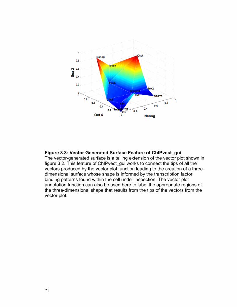
71

Figure 3.3: Vector Generated Surface Feature of ChIPvect_gui The vector-generated surface is a telling extension of the vector plot shown in figure 3.2. This feature of ChIPvect_gui works to connect the tips of all the vectors produced by the vector plot function leading to the creation of a three-dimensional surface whose shape is informed by the transcription factor binding patterns found within the cell under inspection. The vector plot annotation function can also be used here to label the appropriate regions of the three-dimensional shape that results from the tips of the vectors from the vector plot.

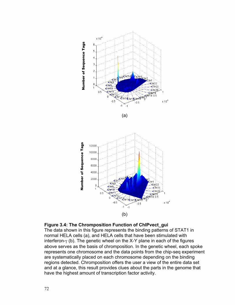
72

(a)

(b)

Figure 3.4: The Chromposition Function of ChIPvect_gui The data shown in this figure represents the binding patterns of STAT1 in normal HELA cells (a), and HELA cells that have been stimulated with interferon-γ (b). The genetic wheel on the X-Y plane in each of the figures above serves as the basis of chromposition. In the genetic wheel, each spoke represents one chromosome and the data points from the chip-seq experiment are systematically placed on each chromosome depending on the binding regions detected. Chromposition offers the user a view of the entire data set and at a glance, this result provides clues about the parts in the genome that have the highest amount of transcription factor activity.

73

Figure 3.5: Chromposition Custom Data Cursor Chromposition is fitted with a custom data cursor that allows the user to obtain information about any data peak in the figure window with the simple click of a button. This custom data cursor provides the chromosome number, chromosome position, and the number of sequence tags/reads associated with each data point.

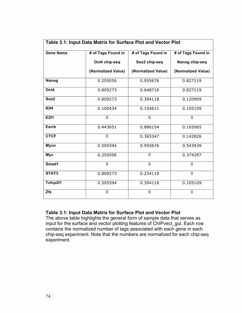
74

Table 3.1: Input Data Matrix for Surface Plot and Vector Plot

Gene Name # of Tags Found in

Oct4 chip-seq

(Normalized Value)

# of Tags Found in

Sox2 chip-seq

(Normalized Value)

# of Tags Found in

Nanog chip-seq

(Normalized Value)

Nanog 0.255056 0.955676 0.827119

Oct4 0.809273 0.648718 0.827119

Sox2 0.809273 0.394118 0.120909

Klf4 0.100434 0.154611 0.105109

E2f1 0 0 0

Esrrb 0.443651 0.886154 0.165065

CTCF 0 0.365347 0.142826

Mycn 0.505594 0.955676 0.543939

Myc 0.255056 0 0.374297

Smad1 0 0 0

STAT3 0.809273 0.234118 0

Tcfcp2I1 0.505594 0.394118 0.105109

Zfx 0 0 0

Table 3.1: Input Data Matrix for Surface Plot and Vector Plot The above table highlights the general form of sample data that serves as input for the surface and vector plotting features of ChIPvect_gui. Each row contains the normalized number of tags associated with each gene in each chip-seq experiment. Note that the numbers are normalized for each chip-seq experiment.

75

Table 3.2: Truncated version of Chromposition Input data matrix Chr # Position # of Tags Chr1 556461 113 Chr1 559591 42 Chr1 703604 29 Chr1 845039 48

.

.

. Chr16 88615427 318 Chr16 88675610 33 Chr17 200296 26 Chr17 259843 39

.

.

. Chr22 48715687 28 Chr22 48730558 49 Chr22 48796845 106 Chr22 48810821 18 Chr22 49127275 47

Table 3.2: Truncated version of Chromposition Input data matrix Each row represents STAT1 binding patterns found in interferon-γ stimulated HELA cells. The first column indicates the chromosome number, the second column contains the mid point of the STAT1 binding range found along the appropriate chromosome, and the third column is simply the number of sequence tags found within that region from the chip-seq experiment.

76

CHAPTER 4

SC Express: A Visual Aid to Identify Single Cells

77

ABSTRACT

Recent developments in microfluidics have made it possible to examine the

expression patterns of single cells via multiplexed quantitative real time PCR.

This powerful technological advance necessitates the development of

bioinformatics tools that can elucidate the unique patterns of gene expression

within a single cell, and facilitate the comparison of gene expression patterns

between cells.

Here we chronicle the design and implementation of SC Express, a MATLAB

based bioinformatics tool that produces a three-dimensional shape that is

reflective of the expression patterns of a single cell. We show that the three-

dimensional shape generated using the genetic contents within a single cell is

reproducible. The software package accepts tab delimited text files containing

the relevant gene expression data and provides a graphical user interface that

enables facile comparison of any two individual cell types on the same screen.

SC Express is a bioinformatics tool that provides a means to visualize gene

expression patterns that are reflective of individual cells.

78

BACKGROUND

Recent developments in microfluidics have made it possible to examine the

expression patterns of single cells (Todd Thorsen, Sebastian J. Maerkl et al.

2002). One of these platforms allows for simultaneous examination of 48

transcripts within 48 isolated single cells with remarkable sensitivity and

reproducibility (Sandra L. Spurgeon, Robert C. Jones et al. 2008). The

technological advances stated above present an opportunity to elucidate the

expression patterns within any single cell and to examine the similarities and

differences between individual cells. There is therefore an emerging need for a

bioinformatics tool that can be used to interpret and categorize the unique and

perhaps subtle signatures of individual cells at a complex molecular level.

In this chapter, the invention of SC Express - a software tool that can be used

to present the expression profiles of individual cells obtained via multiplexed

quantitative real time PCR (qRT-PCR) in a three-dimensional form – is

highlighted. This software package accepts cycle threshold (CT) and fold

enrichment values for 24 transcripts analyzed within 48 single cells. The

software generates a three-dimensional shape for each cell based on the

patterns of gene expression found within it. Technical replicate experiments

performed using the genetic material obtained from the same cell are found to

yield extremely similar three-dimensional shapes when analyzed using SC

Express. These three-dimensional shapes allow for visualization of data, and

79

thus illuminate the subtle expression patterns within a single cell in a way not

possible with more traditional methods. The general principle of SC Express

can be easily applied to the analysis of many other complex data sets such as

chromatin immunoprecipitation coupled with high-throughput sequencing

(ChipSeq), chromatin immunoprecipitation coupled with microarray

(ChIPChip), and RNA sequencing (RNASeq) making the basic principle

behind SC Express of utility for a variety of different methodological

applications.

RESULTS

Application Features: Rendering the Cell Specific 3-D Shapes

SC Express is a tool that can be used to visualize complex transcriptional data

from an individual cell. To test its reliability in depicting these signatures,

human embryonic stem cells (hESCs) were cultured and differentiated towards

definitive endoderm (Thompson, Itskovitz-Eldor et al. 1998; Kevin A D'Amour,

Alan D Agulnick et al. 2005). Single definitive endoderm cells were isolated

using fluorescence activated cell sorting (FACS), lysed, and transcripts within

each single cell were reverse transcribed. After 22 rounds of amplification, 24

different primers representing well-known definitive endoderm genes were

used in qRT-PCR reactions on 48 individual cells using Biomark 48.48TM chips

depicted in Figure 4.1 (Sandra L. Spurgeon, Robert C. Jones et al. 2008). A

80

tab delimited Microsoft excel file containing the resulting CT and fold

enrichment values was used as input data. A truncated version of the input

data file is illustrated in Table 4.1. These CT and fold enrichment values

constitute the numerical basis upon which SC Express generates three-

dimensional shapes for each cell. The representative three-dimensional shape

for each cell is developed in the following way.

First a virtual genetic wheel with lines that emanate from its center and extend

to its circumference is created on the x-y plane in three-dimensional space.

Each line contained in this circle represents one of the 24 genes whose

pattern of expression the user has chosen to examine. Each line is 50 units in

length and is labeled with the symbol of the gene that it represents. A pictorial

representation of the virtual genetic wheel is shown in Figure 4.2a.

After the virtual genetic wheel has been created, SC Express uses the input

data to initiate the second step involved in creating the cell specific three-

dimensional shapes. The input data file takes the form of a two-column matrix

with a variable number of rows (some multiple of 24) depending on how many

individual cells are being examined. The first column of the input data matrix

contains fold enrichment values calculated by the user relative to some set

standard, while the second column contains the CT values recorded by the

48.48 dynamic array system. SC Express breaks apart the input data into

smaller matrices each having a length of precisely 24 rows as illustrated in

81

Table 4.1. These smaller matrices are stored in memory as data that will be

used to create the unique three-dimensional shape for each cell. The first 24

rows of the input data matrix will be used to create the three-dimensional

shape that represents cell 1, with the next 24 being used for cell 2, and so on.

Once the individual matrices have been assigned to each cell the final step

generates a three-dimensional shape for each cell. For each 24 by 2 matrix

representing a single cell, SC Express begins by finding the line on the virtual

genetic wheel that represents the current gene and counts a number of units

along the selected line that corresponds to the rounded CT value associated

with that gene and marks the spot. Next, it creates a stem that rises above the

x-y plane to a height that is equal to the fold enrichment value recorded in the

same row. This stem emanates from the x-y plane at the exact spot that was

previously located using the gene name and the appropriate CT value. This

same procedure is performed for all of the 24 genes selected resulting in a set

of stems in three-dimensional space as shown in Figure 4.2b.

The set of stems constructed as in Figure 4.2b serves as a skeletal

framework upon which the actual three-dimensional shape is built. This part of

SC Express works by connecting the tips of all the stems created to yield a

three-dimensional shape that has been developed by taking the expression

levels of each assayed gene in the single cell into consideration. An example

of a completed cell specific three dimensional shape is illustrated in Figure

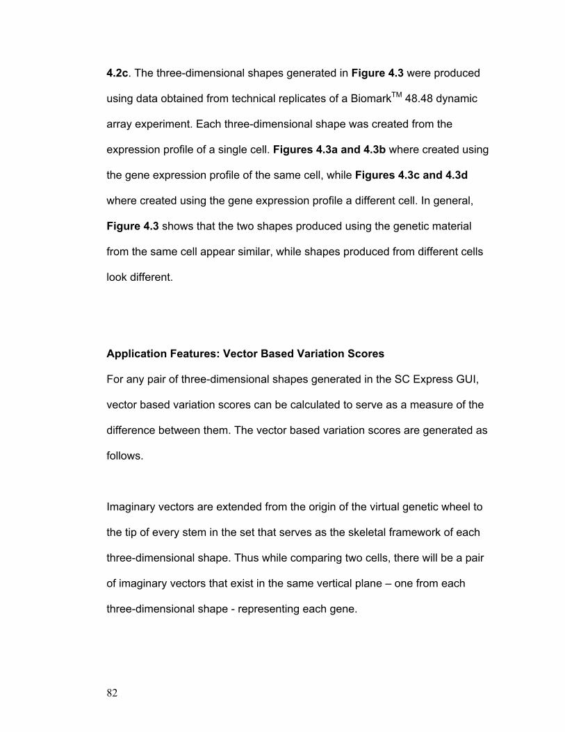
82

4.2c. The three-dimensional shapes generated in Figure 4.3 were produced

using data obtained from technical replicates of a BiomarkTM 48.48 dynamic

array experiment. Each three-dimensional shape was created from the

expression profile of a single cell. Figures 4.3a and 4.3b where created using

the gene expression profile of the same cell, while Figures 4.3c and 4.3d

where created using the gene expression profile a different cell. In general,

Figure 4.3 shows that the two shapes produced using the genetic material

from the same cell appear similar, while shapes produced from different cells

look different.

Application Features: Vector Based Variation Scores

For any pair of three-dimensional shapes generated in the SC Express GUI,

vector based variation scores can be calculated to serve as a measure of the

difference between them. The vector based variation scores are generated as

follows.

Imaginary vectors are extended from the origin of the virtual genetic wheel to

the tip of every stem in the set that serves as the skeletal framework of each

three-dimensional shape. Thus while comparing two cells, there will be a pair

of imaginary vectors that exist in the same vertical plane – one from each

three-dimensional shape - representing each gene.

83

Next, the corresponding sets of imaginary vectors generated for each shape

are compared to obtain a variation score. Specifically, the dot product between

pairs of vectors that represent the same gene in separate three-dimensional

shapes serves as the foundation upon which the variation score is determined.

For the purposes of illustration we will consider two imaginary vectors A1 and

A2 that represent the same gene in different three-dimensional shapes as

shown in Figure 4.4. The variation score between the three-dimensional

shapes being considered for this particular gene is defined as the angle

between vectors A1 and A2 which can be obtained using the dot product of

both vectors as shown in the mathematical formulas below.

A1 . A2 = |A1| |A2| Cos θ (1)

θ = Cos-1 (A1 . A2 / |A1| |A2|) (2)

As the angle between A1 and A2 approaches zero, A1 approaches A2 and vice

versa. For each gene under consideration, an identical procedure is used to

determine the variation between the corresponding pair of imaginary vectors.

SC Express displays the maximum variation score between all corresponding

pairs of vectors, the minimum variation score between all corresponding pairs

of vectors, and the average variation score which is an average measure of

the degree of variation between each pair of corresponding vectors

representing a gene in the pool selected by the user.

84

The variation scores obtained upon comparison of three-dimensional shapes

are also displayed as a stem plot within the GUI. Specifically, the measure of

variation for each gene (in degrees) is plotted as a stem that emanates from

the x-axis. Each stem rises to a height that is exactly equal to the amount of

variation that was calculated for the gene that it represents. This pictorial

representation of the variation in gene expression between any two cells was

designed to give the user a means to discern the particular gene in a chosen

pool that contributes most to the difference between the general expression

patterns of any pair of cells.

Application Features: Graphical User Interface

To ensure the best possible user experience, the software was developed with

a graphical user interface (GUI) on its front end. This GUI is fitted with two

visualization windows that display the three-dimensional shapes generated for

any cell. Drop down menus accompany each visualization window and allow

the user to select the expression data generated for any individual cell. With a

single click of the cell specific 3D plot button, a three-dimensional shape that

represents the selected cell will appear in the appropriate visualization

window. This style fosters an environment in which users can immediately

discern the apparent similarities or differences between any two cells profiled

in the experiment. Figure 4.5 presents a pictorial representation of the SC

Express GUI.

85

DISCUSSION

Current genotyping technology is used to observe gene expression patterns

on a multi-cellular level (Mark Schena, Dari Shalon et al. 1995). The next

frontier is to analyze expression patterns within an individual cell. Technology

is moving quickly toward this goal as indicated by the scientific studies that

have attempted to examine single cell expression (Eberwine, Yeh et al. 1992;

Levsky, Shenoy et al. 2002) the required computational approaches to explore

and analyze this data must keep pace. The relatively recent application of

microfluidics to cell biology has enabled a robust quantitative measure of the

expression patterns within a single cell (Sandra L. Spurgeon, Robert C. Jones

et al. 2008). Here, we report the development of a software tool that can be

used to visualize single cell expression data providing an unprecedented

ability to compare specific patterns of gene expression. SC express provides

resolution of data sets on a single cell level and a level of simplicity that is

unattainable with current bioinformatics tools.

Current bioinformatics analysis techniques such as clustering may allow users

to identify groups of single cells that show closely related patterns of gene

expression, but SC Express offers the added advantage of assigning a unique

three-dimensional signature to each cell. The unique three-dimensional

shapes assigned to each cell allows for direct visual comparison of single cell

specific expression patterns. The apparent reproducibility of these cell specific

86

three-dimensional signatures suggests that they could be used as accurate

markers of cell identity. In addition, SC Express readily calculates maximum,

minimum, and average variation scores between cell specific expression

patterns. The SC express GUI is also fitted with a variation score plot that

depicts the variation in expression for each gene upon comparison of cell

specific three-dimensional shapes. The simplicity of design allows any user

with a basic level of competence in personal computing to examine the

nuances in the expression patterns of a single cell.

SC Express was built to exploit the accuracy and reproducibility of

microfluidics enabled single cell analyses by facilitating visual comparison of

the expression profile of one single cell to another. SC Express’s features

include a GUI front end containing functional push buttons and two

visualization windows within which specific three-dimensional shapes for any

individual cell can be formed. For reasons of familiarity, the program has been

designed to accept tab delimited Microsoft excel files as input data. The above

listed features of the SC Express GUI were made in order to simplify use of

the application and thus tailor it to as wide a range of potential users as

possible.

Although expression data were used to test the efficacy of SC Express, the

basic underlying architecture of SC Express can easily be tailored to a variety

of datasets. Using similar logic, but different parameter assignments, SC

87

Express can generate three-dimensional shapes from ChipSeq or ChipChip

data. Thus the high utility of SC Express makes it a useful platform for

scientists across multiple disciplines to analyze a wide range of diverse

biological datasets.

CONCLUSIONS

SC Express generates three-dimensional shapes that represent the genetic

characteristics of a single cell. Each cell specific three-dimensional shape is

created using the results of 48 RT-qPCR reactions performed on a single cell.

SC Express is designed to give users the freedom to compare individual cells

through the use of three-dimensional shapes that are created using the

genetic characteristics of each cell and provides variation scores that serve as

a measure of variation between any two cell specific three-dimensional

shapes.

IMPLEMENTATION

SC Express is implemented in MATLAB 7. The application can be installed on

local computers in a dedicated sub-directory. SC Express is executed from the

MATLAB 7 prompt by typing in a single command, and providing user defined

names for the input files. Upon execution, the program will prompt the user to

88

provide two tab delimited text files that contain a list of recorded RT-qPCR CT

values and calculated fold enrichments for each and every individual cell

considered in two separate experiments. SC Express is designed to convert

this information into a three-dimensional shape that uniquely represents each

individual cell.

89

Figure 4.1: Biomark 48.48 Dynamic Array Device allows for the execution of 2034 simultaneous qRT-PCR runs on a single chip

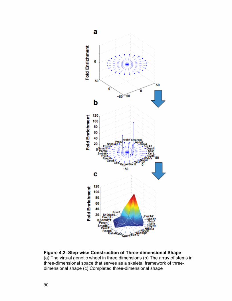
90

Figure 4.2: Step-wise Construction of Three-dimensional Shape (a) The virtual genetic wheel in three dimensions (b) The array of stems in three-dimensional space that serves as a skeletal framework of three-dimensional shape (c) Completed three-dimensional shape

91

Figure 4.3: Three-dimensional cell specific plots Figures (a) and (b) were generated from technical replicate BiomarkTM 48.48 array enabled qRT-PCR experiments performed using cDNA obtained from the same exact single cell: cell 1. (a) Represents the first technical replicate performed using BiomarkTM 48.48 chip number: 1131100054 (b) Represents the second technical replicate performed using BiomarkTM 48.48 chip number: 1131100055. Figures (c) and (d) depict the three dimensional shapes generated using the genetic contents of another cell: cell 4.

92

Figure 4.4: Variation Score between three-dimensional shapes (a) and (b) depict imaginary vectors A1 and A2 that have been drawn to represent the same gene in different three-dimensional shapes. The angle between vectors A1 and A2 serves as the variation score for that particular gene between the three-dimensional shapes being considered.

93

Figure 4.5: SC Express graphical user interface Figure 5.6 shows a screen shot of the SC Express graphical user interface. Visualization windows (A), Cell Specific 3D Plot button (B), Drop down menus (C), Variation score calculator (D), and the Variation Score Plot (E) are all shown in the figure.

94

Cell Gene Symbol Column 1: Fold Enrichment Column 2: CT Value 10 FOXA2 6.317687933 14.81324486

GATA4 2.651446641 16.06909628 APOA2 0.517275768 18.42538484 SMARCD3 0.565844471 18.29420511 NR0B1 4.72631E-05 31.84211789 PRSS2 0.454294384 18.61778746 S100A16 87.57701716 11.02040246 FOXQ1 5.025226082 15.1434441 SAMD11 2.03331E-05 33.16318622 PORCN 2.852996557 15.9604623 SMAD6 3.096406161 15.84283484 PREX1 0.759743641 17.86911417 REEP6 0.689517521 18.00975132 GATA6 24.68464796 12.84709707 GSC 4.177925458 15.40998366 CXCR4 4.114427694 15.43763149 SOX17 2.419376574 16.20095549 MID1IP1 1.489734425 16.89770791 NODAL 27.69063403 12.68135029 NFKBIA 21.63575053 13.03779544 FXYD6 0.25719157 19.43241416 CST3 0.004238115 25.37495379 SOX1 8.65736E-05 31.23749261 GAPDH 100.0469864 10.82877637

Table 4.1: A truncated version of the SC Express input data file The table shows the information contained in the input data matrix. Specifically, the above table shows data recorded for cell #10 in an actual experiment. All 48 cells have such truncated matrix forms, and the complete data file is a concatenation of all 48 truncated matrices arranged with respect to the numerical order of the cells.

95

Chapter 5

Analysis of Gene Expression Patterns in Single Human Embryonic Stem

Cells and Their Derivatives Allows for Cellular Classification

96

ABSTRACT

Background: Discriminating between different cells within complex mixtures is

key to multiple disciplines including stem cell biology, cancer biology, and

developmental biology. Recent developments in microfluidics have made it

possible to examine the expression patterns of single cells via multiplexed

quantitative real time PCR. This powerful technological advance allows for in

depth exploration of the unique patterns of gene expression within a single

cell, and facilitates the comparison of gene expression patterns between cells.

Results: In this report, we demonstrate that transcriptional variation between

isolated single cells is high, but that this variability can be used to clearly

distinguish different cellular types. With the aid of SC Express - a

computational tool that we developed, we show that single isolated endoderm

cells derived from human embryonic stem cells (hESCs) have a surprising

degree of transcriptional variation. Looking closely at this variation, we found

three housekeeping transcripts that change significantly between cell types in

that the relative expression of these three markers when plotted in three-

dimensional space can clearly discriminate between different cellular types,

including 293T, hepg2, induced pluripotent stem cells (iPSCs), hESCs, and

endoderm derived from both iPSCs and hESCs.

Conclusion: Housekeeping transcripts are endemic to all cells, and our study

shows that these transcripts may be useful in discriminating between different

97

cell lines, a finding that could prove useful as a new method of cellular

classification.

98

BACKGROUND

Distinguishing between subtle varieties of cell types is central to many

disciplines, including regenerative medicine and cancer biology. In both fields,

it is essential to identify particular cells within a complex mixture, whether it be

differentiating cultures or tumors. While the transcriptomes of whole

organisms, organ systems and culture regimes, have been described, the

extent of the transcriptional similarities between individual cells within these

populations is far from understood. This distinction is critical, as embryos,

organs, and tumors contain diverse populations of cells. Cell surface receptors

have been highly successful at isolating specific cells from these complex

tissues (Charles M. Baum, Irving L. Weissman et al. 1992), (Kevin A D'Amour,

Alan D Agulnick et al. 2005), but it is likely that cellular complexity is far

greater than a few markers can reflect.

Recent developments in microfluidics have made it possible to examine

the expression patterns of a variety of markers within single cells (Todd

Thorsen, Sebastian J. Maerkl et al. 2002). One of these platforms allows for

simultaneous examination of 48 transcripts within 48 isolated single cells with

remarkable sensitivity and reproducibility (Sandra L. Spurgeon, Robert C.

Jones et al. 2008). The technological advances stated above present an

opportunity to elucidate the expression patterns within any single cell and to

examine the similarities and differences between individual cells.

99

The study of variation between cells may allow insight into lineage

specification. On one hand, the discovery of a finite number of distinct cellular

expression patterns may indicate the existence of cellular subgroups

inherently fated to yield cells of a certain type. On the other hand, extreme

single cell individuality might indicate that transcript levels vary tremendously

between single cells and may not be an indicator of the future identity of a

specific cellular type. Having studied transcriptional variation within purified

hESC derived endodermal cells using recent breakthroughs in microfluidics

(Todd Thorsen, Sebastian J. Maerkl et al. 2002) and a novel bioinformatic

approach termed SCExpress, we find widespread transcriptional variation

between single definitive endoderm cells. This result suggests that these cells

are either highly individualistic or that cellular fate tolerates a high degree of

transcriptional variability. We also found three housekeeping transcripts that

are uncharacteristically variable between definitive endoderm and hESC

populations. Interestingly, the relative expression of these three markers when

plotted in three-dimensional space can clearly discriminate between different

cellular types, including 293T, hepg2, induced pluripotent stem cells (iPSCs),

hESCs, and endoderm derived from both iPSCs and hESCs. These three

transcripts may be used to discriminate different cellular types and may aid

basic biological understanding of lineage formation in hESCs and have

applications in regenerative medicine.

100

RESULTS

Gene Expression Profiling in Single Definitive Endoderm Cells

We hypothesized that expression profiling of single endodermal cells

would enable their classification into specific cellular groups reflective of

different endodermal fates. To this end, we differentiated hESC towards

definitive endoderm using an established differentiation protocol (Kevin A

D'Amour, Alan D Agulnick et al. 2005), and used fluorescence activated cell

sorting (FACS) to isolate cells within the differentiated population that

expressed the chemokine cell surface receptor CXCR4. Next, we selected 22

endoderm specific genes from the intersection of RNA sequencing (RNA-seq)

and exon array experiments performed on these same CXCR4+ definitive

endoderm cells. The endoderm specific genes used in our experiments are

listed in Table 5.1. We added a well-known ectoderm marker (SOX1) and a

housekeeping gene (GAPDH) to the list of genes as controls. Using the

multiplexed quantitative real time PCR (qRT-PCR) BiomarkTM system (Aaron

R. Wheeler, William R. Throndset et al. 2003), we profiled the relative

expression levels of these 24 genes in ~ 80 single CXCR4+ cells. Specifically,

we calculated fold enrichment values by comparing the cycle threshold (CT)

values of each gene to that of the common baseline control: GAPDH. We

found that each CXCR4+ definitive endoderm cell showed a unique pattern of

gene expression as depicted in Figure 5.1a. Even after analyzing the

expression of 22 endoderm specific genes in ~80 CXCR4+ definitive endoderm

101

cells, no two cells displayed identical expression patterns. Thus the transcript

levels of lineage specific molecules during endoderm specification appear to

occur on a continuum.

SC Express: A Tool to Visualize Gene Expression Patterns in Single

Cells

In order to visualize the individual expression patterns of each single

cell, we created SC Express: a method that uses single cell gene expression

to produce three-dimensional shapes . CT values from the Biomark 48.48TM

experiments were used to calculate fold enrichment values using the ΔΔCT

method. The resulting fold enrichment values and original CT values from

which they were calculated were used to create each cell specific three-

dimensional shape using SC Express (See Chapter 4 for a detailed description

of three dimensional shape construction). We found that cell specific three-

dimensional shapes created using our method tend to be individualistic (i.e.

specific to each cell) and reproducible as seen in Figure 5.2. At this point, we

surmised that a more stably expressed class of genes would be better for our

search for patterns that represent distinct cell types.

102

Housekeeping Gene Expression Within Single Cells

Since tissue specific transcripts were highly variable within individual

endoderm cells, we tested housekeeping transcripts to gauge their

consistency in expression within these same cells. While lineage specific

genes appear to be loosely regulated at the transcription level, research has

shown that housekeeping genes are more tightly controlled (Robert D. Barber,

Dan W. Harmer et al. 2005). We selected primers for 22 known housekeeping

genes (Eli Eisenberg and Levanon 2003) listed in Table 5.1 and performed

single cell PCR on FACS isolated SSEA4+ hESC and CXCR4+ hESC derived

endoderm. In general, housekeeping gene expression within single CXCR4+

hESC derived endoderm and single SSEA4+ hESCs was more uniform than

the tissue specific transcripts (Figure 5.1b and 5.1c), suggesting that

housekeeping gene expression is more tightly controlled than those of

regulatory pathways. Interestingly, while the relative level of most of the

housekeeping transcripts appeared to be consistent between hESC and hESC

derived endoderm, a few showed variability.

We also examined the expression of our housekeeping gene set (Table

5.1) within all 6 different cell lines (293T, hepg2, induced pluripotent stem cells

(iPSCs), hESCs, and endoderm derived from both iPSCs and hESCs). During

analysis of housekeeping gene expression in our selected cell lines, we

observed some variation between cells of different types. We performed

103

principal component analysis (PCA) to determine whether certain cell lines

cluster together or diverge based on the expression patterns of our set of

selected housekeeping genes. Our principal component analysis revealed 6

principal components, or axes of variation in the data: PC1, PC2, PC3, PC4,

PC5, and PC6. It should be noted that these principal components are ranked

based on how much variation in the data they explain. For example, principal

component 1 (PC1) explains most of the variation in the data, followed by

PC2, PC3, and so on. The first four principal components account for 87.8% of

the total variation in the dataset (PC1: 33.6%, PC2: 27.2%, PC3: 19.5%, PC4:

7.5%). In general, our data shows that single cells from the same group tend

to have similar housekeeping gene expression patterns resulting in the

formation of clusters of the different cell types (Figure 5.3). The first principal

component – PC1 - separates our hESC cluster from the hepg2 cluster,

marking these two clusters as the most distinct within our dataset (Figure

5.3a). The combination of PC3 and PC4 distinguishes the iPS derived

definitive endoderm from the other cell lines within the group (Figure 5.3b),

and also allows for the emergence of distinct hepG2, and hESCendo clusters.

The combination of PC1 and PC3 isolates iPS endoderm and hepG2 as

distinct clusters within the dataset (Figure 5.3c).

Though the expression patterns of all the genes within our

housekeeping pool yielded good clustering of the different cell lines after

principal component analysis (Figure 5.3), we sought to find the genes that

104

contributed most to the variation between cell lines. To this end, we ranked the

housekeeping genes based on their contribution to the PCA. The

housekeeping genes are listed in Table 5.2 in order of decreasing importance

(1 being the most important, and 24 being the least important) to our PCA.

Since PCA yielded cell type specific clusters based on housekeeping

gene expression, we assessed different permutations of the top 10

contributors to our PCA (Table 5.2) to see if any three of them resulted in

unique clustering of the different cell types. Using the expression patterns of

the top three contributors to our PCA, (LDHA, ACTB, NONO) we performed

principal component analysis again to see if the distinction between clusters of

different cell lines became even more striking relative to the PCA done with

the full set of housekeeping genes. We found that the principal components

derived based on the top three genes (LDHA, ACTB, NONO), were able to

demarcate the cell clusters more effectively (Figure 5.4a). Also, the

combination of LDHA, GPI, and NONO yielded good separation of the cell

clusters after PCA (Figure 5.4b). As a control, we performed PCA using three

genes picked at random from our housekeeping gene set (SOX1, TXN, NCL),

and found that these genes did not clearly separate the different cell types into

distinct clusters as in the case of the top three contributors to the PCA (Figure

5.4c). Further, the top three contributors to the PCA yielded the best visual

separation between the cell lines when the expression patterns of these genes

were used as the X, Y, and Z components for each cell in three-dimensional

105

rectangular coordinates (Figure 5.5a). As a control, we plotted all the different

cell lines in three-dimensional space using the expression patterns of SOX1,

TXN, and NCL as X, Y, and Z components respectively. In this case, the well-

defined cell specific clustering observed for these same cell types using

LDHA, ACTB, NONO as X, Y and Z components was lost.

DISCUSSION

Definitive endoderm cells show remarkable versatility in serving as the

precursor to a multitude of cell types that constitute the visceral organs (Kevin

A D'Amour, Alan D Agulnick et al. 2005; Richard I. Sherwood, Cristian Jitianu

et al. 2007). The developmental versatility of definitive endoderm begs the

question of how homogenous this cell population is on the transcriptional level.

A number of scenarios could arise: single members of this group could be

identical, they could completely differ from one another, or the entire

population could be segregated into sub populations each primed to yield

unique somatic cell types. Answering such questions requires analysis of

lineage specific gene expression patterns on the single cell level. Here, we

show that lineage specific gene expression patterns within single CXCR4+

definitive endoderm cells are highly individualistic. Several theories could

explain the unique patterns of lineage specific gene expression observed in

each endoderm cell. In one scenario, the expression level of each lineage

specific gene may only need to exceed a certain threshold for the cells to

attain endodermal fate. In this model, cellular identity may be controlled by

106

posttranscriptional mechanisms. Studies have shown that protein levels within

a cell can be modulated by intricate posttranscriptional mechanisms

(Nishimoto T 1981). These posttranscriptional mechanisms may act to keep

the amount of lineage specific proteins produced within a range that confers

endodermal character. Therefore, though the pattern of endoderm specific

genes expressed from cell to cell appears to be stochastic, the developmental

potential of each cell may be identical due to similar levels of protein

expression. If this were indeed the correct mechanism of gene expression

regulation, housekeeping genes appear to be exempt from this method of

control. The pattern of housekeeping gene expression that we discovered is

tightly controlled and does not appear to require this mode of regulation.

In a second scenario, transcript variation may reflect the actual

diversity, vast plasticity and developmental potential of definitive endoderm.

Fate mapping studies during mouse embryo development suggest that cellular

sub groups within definitive endoderm are inherently fated to yield cells of a

given type (Kristie A. Lawson, Juanito J. Meneses et al. 1991; Kimberly D.

Tremblay and Zaret 2005). On the other hand, co-culture experiments in the

embryo show that endoderm is not fully committed to any lineage in the early

stages of development (James M. Wells and Melton 2000). These studies in

addition to our own findings suggest that precursor cells within a given lineage

are not irreversibly fated to give rise to defined cell types. The transcriptional

heterogeneity observed within the definitive endoderm population is more

107

supportive of a developmental model in which each cell has some potential to

develop into a handful of cell types, but the eventual fate decision is pliable

and ultimately cemented by the presence of unique permutations of

developmental factors in the right concentration, at the right place and time.

This might be particularly true of endoderm derived in culture since the precise

inductive interactions characteristic of the three-dimensional embryo are not

present. We investigated endodermal heterogeneity within the embryo proper,

but were unable to consistently isolate single live endoderm cells from the

embryo. Thus, it is unclear whether transcript variability is specific to in vitro

differentiation conditions using hESCs. Nonetheless, this heterogeneity is a

critical issue to be understood when producing cell types for regenerative

medicine applications.

We have also shown through principal component analysis that

housekeeping gene expression is unique enough between different cell types

to result in the formation of distinct clusters. Further, we discovered three

housekeeping genes within our selected pool with sufficient variability in their

patterns of expression to distinguish between six different cell lines, including

hESCs and iPSCs. Although housekeeping genes have traditionally been

used to normalize gene expression data, recent work has shown that the

expression of this class of genes may vary from cell to cell (Luigi Warren,

David Bryder et al. 2006). Our work expands on this observation and

suggests that the variation in housekeeping transcripts could be an untapped

108

resource with which to distinguish different cell types, and could be an

important tool for both regenerative medicine and clinical diagnostics. For

example, variation in housekeeping gene expression could be used as a tool

to select specialized cell types from differentiating culture. It could also serve

as a possible diagnostic to distinguish between cancerous and non-cancerous

cells of the same cell type. In the future, it would be interesting to examine the

expression patterns of all housekeeping genes within as many different cells

as possible in search of a subset whose patterns of expression can be used to

distinguish between them. In general, single cell gene expression data is

immensely powerful and holds great promise for the study of development,

disease progression, and the treatment of disease.

109

Figure 5.1: Gene expression profiles within CXCR4+ definitive endoderm and SSEA4+ hESC. Expression patterns of endoderm specific and housekeeping genes are shown. Each panel contains ~40 traces with each trace representing the expression patterns of a single cell. (a): Endoderm specific genes are uniquely expressed in each CXCR4+ definitive endoderm cell. (b): Relative to lineage specific genes, housekeeping gene expression patterns within single definitive endoderm cells are much more uniform. (c): Housekeeping genes are also uniformly expressed in a group of single SSEA4+ human embryonic stem cells

110

Figure 5.2: Single cell specific three-dimensional shapes representing unique patterns of endoderm specific gene expression within CXCR4+ definitive endoderm cells The same CXCR4+ endoderm cell was used to generate (a) and (b) above. A separate CXCR4+ endoderm cell was used to generate (c) and (d) above. These shapes show that three dimensional shapes generated using endoderm specific gene expression patterns within the same single cells are highly reproducible, though the pattern of expression for these genes within single cells is unique.

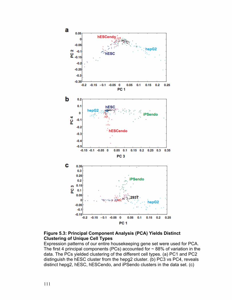
111

Figure 5.3: Principal Component Analysis (PCA) Yields Distinct Clustering of Unique Cell Types Expression patterns of our entire housekeeping gene set were used for PCA. The first 4 principal components (PCs) accounted for ~ 88% of variation in the data. The PCs yielded clustering of the different cell types. (a) PC1 and PC2 distinguish the hESC cluster from the hepg2 cluster. (b) PC3 vs PC4, reveals distinct hepg2, hESC, hESCendo, and iPSendo clusters in the data set. (c)

112

PC3 vs PC1 results in the emergence of distinct iPSendo, hepG2, and 293T clusters.

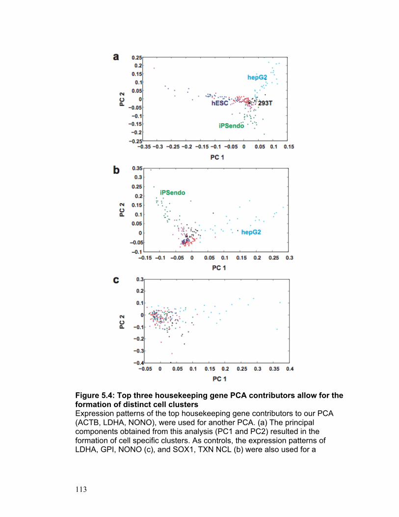
113

Figure 5.4: Top three housekeeping gene PCA contributors allow for the formation of distinct cell clusters Expression patterns of the top housekeeping gene contributors to our PCA (ACTB, LDHA, NONO), were used for another PCA. (a) The principal components obtained from this analysis (PC1 and PC2) resulted in the formation of cell specific clusters. As controls, the expression patterns of LDHA, GPI, NONO (c), and SOX1, TXN NCL (b) were also used for a

114

separate PCA. The resulting plots (b) and (c) show that the clusters loose distinction in each of the two cases.

115

Figure 5.5: Plotting the expression patterns of the top three contributors to our PCA (ACTB, LDHA, NONO) results in the formation of cell specific clusters that can be visually distinguished from one another. Each cell is represented in three-dimensional space using the expression patterns of ACTB, LDHA, and NONO as X,Y and Z components respectively. This results in the formation of well defined cell specific clusters in three-dimensional space.

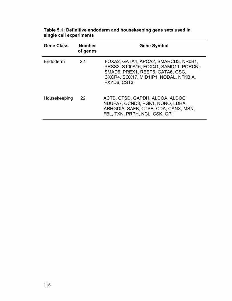
116

Table 5.1: Definitive endoderm and housekeeping gene sets used in single cell experiments Gene Class Number Gene Symbol of genes Endoderm 22 FOXA2, GATA4, APOA2, SMARCD3, NR0B1,

PRSS2, S100A16, FOXQ1, SAMD11, PORCN, SMAD6, PREX1, REEP6, GATA6, GSC, CXCR4, SOX17, MID1IP1, NODAL, NFKBIA, FXYD6, CST3

Housekeeping 22 ACTB, CTSD, GAPDH, ALDOA, ALDOC, NDUFA7, CCND3, PGK1, NONO, LDHA, ARHGDIA, SAFB, CTSB, CDA, CANX, MSN, FBL, TXN, PRPH, NCL, CSK, GPI

117

Table 5.2: Ranking the housekeeping genes in order of decreasing significance to the principal component analysis Rank Gene Symbol

1 ACTB 2 NONO 3 LDHA 4 NCL 5 TXN 6 GPI 7 CSTD 8 CANX 9 PGK1 10 CSTB 11 MSN 12 NDUFA7 13 SAFB 14 ARHGDIA 15 FBL 16 ALDOC 17 CCND3 18 ALDOA 19 CDA 20 PRPH 21 CSK

118

MATERIALS AND METHODS hESC Maintenance

hESCs were maintained in mouse embryonic fibroblast conditioned media on

10cm tissue culture plates (BD Falcon) coated with matrigel (R&D). The media

consists of DMEM F-12 (GIBCO), 20% Knockout serum (GIBCO), Non-

essential amino acids (GIBCO), 4ng/ml basic fibroblast growth factor

(peprotech), L-Glutamine (GIBCO), and β-mercaptoethanol. The media was

conditioned by MEFs for 24 hours at 37oC in 5% CO2. Cells were fed every 24

hours, and passed every 4 – 5 days.

iPS Maintenance iPS cells were maintained on mouse embryonic feeder layers in DMEM F-12

(GIBCO) supplemented with 20% knockout serum (GIBCO), non-essential

amino acids, 8ng/ml basic fibroblast growth factor (peprotech), L-glutamine,

and β-mercaptoethanol. Cell culture media was replaced daily, and cells were

passed in a 1:3 ratio every 4 – 5 days

hESC and iPS Cell Differentiation

hESCs were differentiated to definitive endoderm using the TGF-β signaling

molecule activin A. hESC media was aspirated and the cells were washed in

PBS (GIBCO) to remove any lingering traces of serum. Differentiation was

carried out in RPMI (GIBCO) containing 100ng/ml of activin A, and defined

FBS (Hyclone). The concentration of FBS in the solution was steadily

increased during differentiation from 0% for the first 24h, 0.2% for the next

24h, and 2% for all subsequent days of differentiation.

iPS cells were differentiated in much the same way as hESCs using the TGF-β

signaling molecule activin A. Differentiation was carried out in RPMI containing

100ng/ml of activin A, and defined fetal bovine serum (Hyclone). The

concentration of fetal bovine serum in the solution was steadily increased

119

during differentiation from 0% for the first 24h, 0.2% for the next 24h, and 2%

for all subsequent days of differentiation.

Tissue Culture: 293T 293T cells were cultured on 15cm dishes in DMEM (GIBCO) supplemented

with 10% FBS (GIBCO) and 1% penicillin streptomycin. Media was replaced

every 2 days. Cells were harvested by trypsinization for subsequent lysis,

amplification, and Biomark experiments.

Tissue Culture: HepG2 HepG2 cells were cultured in T175 flasks (BD Falcon) in DMEM cell culture

media (GIBCO) supplemented with 10% FBS (GIBCO) and 1% penicillin

streptomycin (GIBCO). Media was replaced every 2 days and cells were

harvested via trypsinization for subsequent amplification and Biomark

experiments.

FACS

Definitive endoderm cells were washed with PBS to remove any traces of

serum, and harvested using 0.05% trypsin/EDTA (GIBCO). Cells were briefly

washed in PBS and then again in Stain Buffer (BD Pharmigen). Human serum

substitute (Irvine Scientific) was added to prevent non-specific binding.

Endoderm cells were stained using monoclonal phycoerythrin labeled

antibodies against CXCR4 (R&D) for 30 – 45 minutes. After staining, cells

were washed twice in BD stain buffer, and resuspended in PBS. Single

definitive endoderm cells were sorted into individual wells of low profile 96 well

plates (Thermo Scientific) containing 5ul of Cells Direct 2x reaction mix

(Invitrogen) and SUPERase-In (Applied Biosystems) per well. The FACS

experiments were carried out at the Stanford FACS facility using BD FACS

Aria equipment. hESCs were sorted with the same protocol used to sort

definitive endoderm. However in the case of hESCs, monoclonal anti-human

120

allophycocyanin labeled antibodies against SSEA4 (R&D) were used to isolate

single hESCs into each well of low profile 96 well plates.

Biomark 48.48 Experiments

Immediately after cell sorting, cells were lysed, mRNA was reverse transcribed

(at 50oC for 15 minutes), and the resulting cDNA was amplified using Taqman

Primers (Applied Biosystems) specific to our selected gene set. The genetic

material from this pre-amplification step was diluted in a 1:4 ratio with TE

buffer (IDT). The diluted cDNA product was combined with Fluidigm’s Sample

loading reagent developed specifically for multiplexed quantitative real time

PCR (qRT-PCR) using the Biomark 48.48TM system. The Taqman assay for

each analyzed gene was mixed with Fluidigm’s Assay loading reagent in a 1:1

ratio in preparation for the qRT-PCR experiment. 5ul of each cDNA sample

mixture and 5ul of each Taqman assay mixture were distributed into the

appropriate wells on the 48.48 microfluidic chip. The chip was then primed and

loaded using the Biomark Nanoflex integrated fluidic chip controller, and

inserted into the Biomark machine for multiplexed qRT-PCR.

Principal Component Analysis Principal components analysis (PCA) is a linear dimensionality reduction

method that is widely used in population genetic studies. The technique seeks

to identify a small number of components that together account for most of the

variation in the data. Given an m x n matrix X of data for m cells at n loci, it is

common practice to perform PCA on the covariance matrix, estimated from the

data as follows:

where µX is the vector of average expression for each individual over all

genes.

121

Sample preparation

PCA can be highly influenced by outlier individuals. Thus, we first opted to

screen out cells with possibly aberrant expression profiles at one or more

housekeeping genes used in the study. To this end, we examined the

distribution of expressions over all cells at each gene; we then systematically

excluded cells whose expression level at any one gene deviated from the

average expression at that locus by more than 10 standard deviations. This

process resulted in the exclusion of 3 cells, bringing the total sample size in

this analysis to 189.

Treatment of missing data

Of the 189 remaining cells, only 6 were found to be missing expression data at

one or more genes. Of these, 5 had missing information for only one of the 24

housekeeping genes; the remaining cell had missing information at two loci.

To compute the covariance matrix as described above, we first set the

expression of the missing genes in these cells to 0. To correct for biases that

may result from these missing data, we then normalized the entries of the

covariance matrix by the number of non-missing genes used to estimate the

covariance in expression between every pair of cells. In other words, for each

entry we now have:

where nij is the number of genes that are non-missing in both cells i and j.

Identification of PCA-correlated genes

To identify a subset of genes that best explains the variation in the data, we

adopted a method described in the context of genome-wide human genetic

studies (Paschou, Ziv et al. 2007). This technique, aims to select a small set of

SNPs that best capture the intricate genetic relationships between human

populations, and is readily applicable to our dataset. Briefly, their algorithm

122

determines the number of significant principal components derived from the

data. These principal components are then used to compute an importance

score for each locus; the markers with the highest scores are those with

highest correlation to the PCA. We now describe how these steps were

applied to the single cell data in this study.

Identifying significant principal components

Estimating the number of significant PCs is an area of active research in

Random Matrix Theory. The original paper from Paschou et al. suggests

comparing the structure of the matrix corresponding to each PC and all

smaller ones to that of a random matrix constructed from the same entries. A

cutoff is then specified, and principal components that exhibit more structure

than the resulting random ones are retained as significant. While this method

enjoys the advantage of being computationally fast and straightforward to

implement, it tends to overestimate the number of significant PCs.

Another approach draws from the observation that, for a suitably normalized m

x n rectangular matrix, the eigenvalues of the PCA are approximately Tracy-

Widom distributed for large m and n (Johnstone 2001; Patterson, Price et al.

2006). Quantiles from the Tracy-Widom distribution have been computed in a

number of studies and are readily available (Matlab), and thus one could in

theory use the distribution to compute p-values for all of our PCs. In practice

however, the fact that our study focuses on a very small number of genes (24

loci) invalidates the assumption that the Tracy-Widom approximation would

hold in this case.

To circumvent these limitations, we opted instead to retain the first few

principal components that together explain a certain arbitrary proportion of the

variance in the data. We find that the first 4 principal components account for

99% of the variance in the data. This observation was corroborated by plots of

PC4 versus PC5 and PC5 versus PC6, which together did not appear to

123

capture any of the structure in the data (not shown). Thus, we elected to use

the first 4 principal components to obtain the importance scores for our

housekeeping genes.

Computation of importance scores

The single value decomposition theorem states that any rectangular m x n

matrix can be decomposed into a factorization of the form:

Hence, in vector notation, the data matrix can be written as the sum:

where di is the ith eigenvalue, and ui and vi are the ith columns of matrices U

and V, respectively. Paschou et al. argue then that the SNPs that have the

largest effects on the PCs should have large coefficients vi; they therefore

propose the importance score (Paschou, Ziv et al. 2007):

where k is now the number of significant PCs retained for the analysis (in our

case, k=4).

To determine which subset of genes has the greatest influence on our PCA,

we proceeded in two steps. We first removed all 6 cells with missing data and

used the statistical package R to obtain the singular value decomposition of

the data matrix. Finally, using the right singular matrix, we used the above

equation to compute importance scores for all 24 housekeeping genes.

124

CHAPTER 6

Outlook

125

As mankind continues to unravel the mysteries of mammalian

development, it is becoming increasingly apparent that studying the

mechanics involved in the control of gene expression on both the multi-cellular

and unicellular levels is of utmost importance. In recent times, tools with which

to extensively study the dynamics of gene expression have been developed.

Technological advances such as the DNA microarray and second generation

sequencing instruments - the Illumina Genome Analyzer, the HeliScope single

molecule sequencer, and Life Technologies’ SOLiD 4 - have provided a

means to gauge the expression patterns of any cell type, organ or tissue with

unprecedented accuracy and depth. These new technologies have spawned

an era in which expression profiling of different cell groups, whole transcript

sequencing, the study of transcription factor occupancy, and even whole

genome sequencing are now possible (Jackson, Bartz et al. 2003; Johnson,

Mortazavi et al. 2007; Pushkarev, Neff et al. 2009). While the above

mentioned instruments are immensely powerful, they are mostly limited to

addressing scientific questions on a multi-cellular scale.

On a smaller but equally significant scale, methods have been

established to examine gene expression patterns within single cells (Levsky,

Shenoy et al. 2002; Aaron R. Wheeler, William R. Throndset et al. 2003;

Sandra L. Spurgeon, Robert C. Jones et al. 2008). These efforts have

culminated in robust systems such as the BiomarkTM which can readily assay

the expression of as many as 48 genes within 48 single cells. These single

126

cell gene expression assay platforms answer many of the same questions as

the second generation sequencing platforms, but on a higher level of

resolution. With these new single cell ready platforms, it has now become

possible to examine questions concerning the genetic similarity and

differences between single cells of the same type, or between cells of different

types (Guo, Huss et al. 2010).

The marriage of second generation sequencing and single cell analysis

is an extremely important avenue for the study of development. With

microarrays and second generation sequencing instruments, it is possible to

asses the average global measure of gene expression within a group of cells

as they progress from naivety to a more determined state (Richard I.

Sherwood, Cristian Jitianu et al. 2007). On the other hand, single cell gene

expression instruments can be used to examine each cell within the transient

cell populations formed as naïve cell groups mature (Guo, Huss et al. 2010).

Using these two powerful technologies in tandem, we can now unequivocally

determine if the average expression pattern found on the multi-cellular scale is

representative of each individual cell, or rather, just an average measure of the

gene expression patterns seen on the unicellular level.

Answering questions pertaining to cellular diversity within a given cell

group is key to the budding disciplines of regenerative medicine and tissue

engineering. In these related fields, it is important to obtain pure populations of

127

therapeutically relevant cell types for implantation into an afflicted individual.

To ensure safety of the recipient/patient in this case, the identity of the cells

being implanted for therapeutic reasons must be unequivocally determined.

With the burgeoning toolkit of biotech instruments currently available, it is

becoming possible to determine the identity of the members of any group of

cells. This obviously bodes well for the field of cell replacement therapy, where

replacing specific diseased cells to restore a particular function within a

diseased patient is the ultimate goal.

The efforts in this thesis have been mainly directed towards using

second generation sequencing instruments to understand the epigenetic

changes that occur as hESCs become more determined, and elucidating the

gene expression patterns in cells that have been derived from hESCs on a

single cell level. This powerful combination of genetic analysis on the multi-

cellular and the unicellular level is what I hope is the beginning of larger scale

efforts to characterize therapeutically relevant cell types obtained from hESCs,

to ensure the safety of potential cell replacement therapy patients in the future.

128

CHAPTER 7

Archive: MATLAB CODE

129

%%%%%%%%%%%%%%%%%%%%%%%%%%%%%%%%% %%%%%%%%%%%%%%%%%%%%%%%%%%%%%%%%% % ChIPvect GUI PROGRAM CODE % % Created By Chuba B. Oyolu % % Date: 07/29/2008 % % Last Modified: 06/21/2009 % %%%%%%%%%%%%%%%%%%%%%%%%%%%%%%%%% %%%%%%%%%%%%%%%%%%%%%%%%%%%%%%%%% function varargout = chipvect_gui(varargin) %CHIPVECT_GUI M-file for chipvect_gui.fig %CHIPVECT_GUI, by itself, creates a new CHIPVECT_GUI or raises the %existing singleton*. %H = CHIPVECT_GUI returns the handle to a new CHIPVECT_GUI or the %handle to the existing singleton*. %CHIPVECT_GUI('CALLBACK',hObject,eventData,handles,...) calls the local %function named CALLBACK in CHIPVECT_GUI.M with the given input %arguments. %CHIPVECT_GUI('Property','Value',...) creates a new CHIPVECT_GUI or %raises the existing singleton*. Starting from the left, property value %pairs are applied to the GUI before chipvect_gui_OpeningFunction gets %called. An unrecognized property name or invalid value makes property %application stop. All inputs are passed to chipvect_gui_OpeningFcn via %varargin. %*See GUI Options on GUIDE's Tools menu. Choose "GUI allows only one %instance to run (singleton)".See also: GUIDE, GUIDATA, GUIHANDLES %Edit the above text to modify the response to help chipvect_gui %Last Modified by GUIDE v2.5 05-Feb-2009 09:39:40 %****************Begin initialization code - DO NOT EDIT***********% gui_Singleton = 1; gui_State = struct('gui_Name', mfilename, ... 'gui_Singleton', gui_Singleton, ... 'gui_OpeningFcn', @chipvect_gui_OpeningFcn, ... 'gui_OutputFcn', @chipvect_gui_OutputFcn, ... 'gui_LayoutFcn', [] , ... 'gui_Callback', []); if nargin && ischar(varargin{1}) gui_State.gui_Callback = str2func(varargin{1}); end if nargout [varargout{1:nargout}] = gui_mainfcn(gui_State, varargin{:}); else gui_mainfcn(gui_State, varargin{:}); end %**************End initialization code - DO NOT EDIT***************%

130

%Executes just before chipvect_gui is made visible. function chipvect_gui_OpeningFcn(hObject, eventdata, handles, varargin) %This function has no output args, see OutputFcn. %hObject - handle to figure %eventdata - reserved - to be defined in a future version of MATLAB %handles - structure with handles and user data (see GUIDATA) %varargin - command line arguments to chipvect_gui (see VARARGIN) %Import the file from Microsoft Excel... filename1 = input('Please Enter Filename: ','s'); chipmat = xlsread(['/Applications/MATLAB_SV74/' filename1 '.xls']); %User Input for axis labels... labelx = input('Please Label X axis: ','s'); labely = input('Please Label Y axis: ','s'); labelz = input('Please Label Z axis: ','s'); filename2 = input('Please Enter Filename For Chromposition: ','s'); raw_data = dlmread(['/Applications/MATLAB_SV74/' filename2 '.txt']); %Ensure that the file is the right size... if size(chipmat) ~= [12 3]; error('INVALID MATRIX SIZE... MATRIX DIMENSIONS MUST BE 12 rows X 3 columns'); return end zero_vect = [0 0 0]; %Data for Surface Plot... handles.surf = chipmat; %Data for Vector Arrow Plot... handles.vectarrow = chipmat; %Data for Vector generated surface... handles.vectgen = chipmat; %Data for Chromposition... handles.chromposition = raw_data; %Data for Chrompeaks... handles.chrompeaks = raw_data; %Label for the x,y, and z axes handles.labelx =labelx; handles.labely =labely; handles.labelz =labelz; %%%%%%%%%%%%%%%%%%%%%%%%%%%%%%%%%%%%%%%%%%%%% % Default is to start with the surface plot % %%%%%%%%%%%%%%%%%%%%%%%%%%%%%%%%%%%%%%%%%%%%% handles.current_data = handles.surf; surf(handles.current_data); title('Matrix Generated 3D-Surface Plot'); shading interp; %Choose default command line output for chipvect_gui

131

handles.output = hObject; %Update handles structure guidata(hObject, handles); %UIWAIT makes chipvect_gui wait for user response (see UIRESUME) %uiwait(handles.figure1); %Outputs from this function are returned to the command line. function varargout = chipvect_gui_OutputFcn(hObject, eventdata, handles) %varargout cell array for returning output args (see VARARGOUT); %hObject handle to figure %eventdata reserved - to be defined in a future version of MATLAB %handles structure with handles and user data (see GUIDATA) %Get default command line output from handles structure varargout{1} = handles.output; %%%%%%%%%%%%%%%%%%%%%%%%%%%%%%%%%%%%%%%%%%%%%%%%%%%%% % Button press in pushbutton1 (Surface Plot Button) % %%%%%%%%%%%%%%%%%%%%%%%%%%%%%%%%%%%%%%%%%%%%%%%%%%%%% function pushbutton1_Callback(hObject, eventdata, handles) %hObject - handle to pushbutton1 (see GCBO) %eventdata - reserved - to be defined in a future version of MATLAB %handles - structure with handles and user data (see GUIDATA) surf(handles.current_data); title('Matrix Generated 3D-Surface Plot'); shading interp; rotate3d off %%%%%%%%%%%%%%%%%%%%%%%%%%%%%%%%%%%%%%%%%%%%%%%%%%%% % Button press in pushbutton2 (Vector Plot Button) % %%%%%%%%%%%%%%%%%%%%%%%%%%%%%%%%%%%%%%%%%%%%%%%%%%%% function pushbutton2_Callback(hObject, eventdata, handles) %hObject - handle to pushbutton2 (see GCBO) %eventdata - reserved - to be defined in a future version of MATLAB %handles - structure with handles and user data (see GUIDATA) j = 1; zero_vect = [0 0 0]; for j = 1:length(handles.current_data); if j > length(handles.current_data); break; else vectarrow(zero_vect,handles.current_data(j,:)); hold on; j = j + 1; xlabel(handles.labelx); ylabel(handles.labely); zlabel(handles.labelz); end end hold off; rotate3d off

132

title('Matrix Generated 3D-Vector Plot'); %%%%%%%%%%%%%%%%%%%%%%%%%%%%%%%%%%%%%%%%%%%%%%%%%%%%%%%%%%%%%%%%%%% % Check in Checkbox Right Below Vector Plot (Annotate Vector Plot)% %%%%%%%%%%%%%%%%%%%%%%%%%%%%%%%%%%%%%%%%%%%%%%%%%%%%%%%%%%%%%%%%%%% function checkbox1_Callback(hObject,eventdata,handles) %Define Vector that contains the names of all genes being considered genevect = {'Nanog';'Oct4';'Sox2';'klf4';'E2f1';'Esrrb';'CTCF'; 'Mycn';'Myc';'Smad1';'STAT3';'Tcfcp2I1';'Zfx';'Gene 14'}; nullvect = {'';'';'';'';'';'';'';'';'';'';'';'';'';''}; checkboxStatus = get(handles.checkbox1,'Value'); k = 1; if checkboxStatus == 1; for k = 1:length(handles.current_data); text(handles.current_data(k,1),handles.current_data(k,2),handles.current_data(k,3),genevect(k)); hold on; k = k + 1; end end hold off; if checkboxStatus == 0; for k = 1:length(handles.current_data); text(handles.current_data(k,1),handles.current_data(k,2),handles.current_data(k,3),nullvect(k)); hold on; k = k + 1; end end hold off; %%%%%%%%%%%%%%%%%%%%%%%%%%%%%%%%%%%%%%%%%%%%%%%%%%%%%%%%%%%%%%%%% % Button press in pushbutton3 (Vector Generated Surface Button) % %%%%%%%%%%%%%%%%%%%%%%%%%%%%%%%%%%%%%%%%%%%%%%%%%%%%%%%%%%%%%%%%% function pushbutton3_Callback(hObject, eventdata, handles) %hObject - handle to pushbutton3 (see GCBO) %eventdata - reserved - to be defined in a future version of MATLAB %handles - structure with handles and user data (see GUIDATA) x = handles.current_data(:,1); y = handles.current_data(:,2); z = handles.current_data(:,3); tri = delaunay(x,y); h = trisurf(tri,x,y,z); shading interp; lighting phong;

133

xlabel(handles.labelx); ylabel(handles.labely); zlabel(handles.labelz); rotate3d off title('Vector Generated 3D-Surface'); %%%%%%%%%%%%%%%%%%%%%%%%%%%%%%%%%%%%%%%%%%%%%%%%%%%%%%%%%%%%%%%% % Button press in pushbutton4 (Enable 3D Plot Rotation Button) % %%%%%%%%%%%%%%%%%%%%%%%%%%%%%%%%%%%%%%%%%%%%%%%%%%%%%%%%%%%%%%%% function pushbutton4_Callback(hObject, eventdata, handles) %hObject - handle to pushbutton4 (see GCBO) %eventdata - reserved - to be defined in a future version of MATLAB %handles - structure with handles and user data (see GUIDATA) rotate3d on %%%%%%%%%%%%%%%%%%%%%%%%%%%%%%%%%%%%%%%%%%%%%%% % Button press in pushbutton6 (Chromposition) % %%%%%%%%%%%%%%%%%%%%%%%%%%%%%%%%%%%%%%%%%%%%%%% function pushbutton6_Callback(hObject, eventdata, handles) %hObject - handle to pushbutton6 (see GCBO) %eventdata - reserved - to be defined in a future version of MATLAB %handles - structure with handles and user data (see GUIDATA) cursor_mat = handles.chromposition; handles.chromposition(:,2) = (handles.chromposition(:,2)/max(handles.chromposition(:,2)))*10000; handles.chromposition(:,2) = round(handles.chromposition(:,2)); %Generating the Points on the circle... NOP = 23; radius_circ = max(handles.chromposition(:,2)); center = [0,0,10]; style = '.'; global radius_circ; THETA=linspace(0,2*pi,NOP); RHO=ones(1,NOP)*radius_circ; [X,Y] = pol2cart(THETA,RHO); X=X+center(1); Y=Y+center(2); Z = center(3)*ones(1,length(X)); H=plot3(X,Y,Z,style); xlabel('x coordinate'); ylabel('y coordinate'); zlabel('Number Of Reads'); axis square; grid

134

%Creating the spokes of the bicycle wheel... chuba = [X,Y]; emeka = [chuba(:,1:23);chuba(:,24:46)]; coord_mat = emeka'; line([0 coord_mat(1,1)],[0 coord_mat(1,2)],[10 10],'Marker','.','LineStyle','--'); line([0 coord_mat(2,1)],[0 coord_mat(2,2)],[10 10],'Marker','.','LineStyle','--'); line([0 coord_mat(3,1)],[0 coord_mat(3,2)],[10 10],'Marker','.','LineStyle','--'); line([0 coord_mat(4,1)],[0 coord_mat(4,2)],[10 10],'Marker','.','LineStyle','--'); line([0 coord_mat(5,1)],[0 coord_mat(5,2)],[10 10],'Marker','.','LineStyle','--'); line([0 coord_mat(6,1)],[0 coord_mat(6,2)],[10 10],'Marker','.','LineStyle','--'); line([0 coord_mat(7,1)],[0 coord_mat(7,2)],[10 10],'Marker','.','LineStyle','--'); line([0 coord_mat(8,1)],[0 coord_mat(8,2)],[10 10],'Marker','.','LineStyle','--'); line([0 coord_mat(9,1)],[0 coord_mat(9,2)],[10 10],'Marker','.','LineStyle','--'); line([0 coord_mat(10,1)],[0 coord_mat(10,2)],[10 10],'Marker','.','LineStyle','--'); line([0 coord_mat(11,1)],[0 coord_mat(11,2)],[10 10],'Marker','.','LineStyle','--'); line([0 coord_mat(12,1)],[0 coord_mat(12,2)],[10 10],'Marker','.','LineStyle','--'); line([0 coord_mat(13,1)],[0 coord_mat(13,2)],[10 10],'Marker','.','LineStyle','--'); line([0 coord_mat(14,1)],[0 coord_mat(14,2)],[10 10],'Marker','.','LineStyle','--'); line([0 coord_mat(15,1)],[0 coord_mat(15,2)],[10 10],'Marker','.','LineStyle','--'); line([0 coord_mat(16,1)],[0 coord_mat(16,2)],[10 10],'Marker','.','LineStyle','--'); line([0 coord_mat(17,1)],[0 coord_mat(17,2)],[10 10],'Marker','.','LineStyle','--'); line([0 coord_mat(18,1)],[0 coord_mat(18,2)],[10 10],'Marker','.','LineStyle','--'); line([0 coord_mat(19,1)],[0 coord_mat(19,2)],[10 10],'Marker','.','LineStyle','--'); line([0 coord_mat(20,1)],[0 coord_mat(20,2)],[10 10],'Marker','.','LineStyle','--'); line([0 coord_mat(21,1)],[0 coord_mat(21,2)],[10 10],'Marker','.','LineStyle','--'); line([0 coord_mat(22,1)],[0 coord_mat(22,2)],[10 10],'Marker','.','LineStyle','--'); line([0 coord_mat(23,1)],[0 coord_mat(23,2)],[10 10],'Marker','.','LineStyle','--'); hold on;

135

%Labelling the Chromosomes... text(coord_mat(1,1),coord_mat(1,2),10,'Chr1'); text(coord_mat(2,1),coord_mat(2,2),10,'Chr2'); text(coord_mat(3,1),coord_mat(3,2),10,'Chr3'); text(coord_mat(4,1),coord_mat(4,2),10,'Chr4'); text(coord_mat(5,1),coord_mat(5,2),10,'Chr5'); text(coord_mat(6,1),coord_mat(6,2),10,'Chr6'); text(coord_mat(7,1),coord_mat(7,2),10,'Chr7'); text(coord_mat(8,1),coord_mat(8,2),10,'Chr8'); text(coord_mat(9,1),coord_mat(9,2),10,'Chr9'); text(coord_mat(10,1),coord_mat(10,2),10,'Chr10'); text(coord_mat(11,1),coord_mat(11,2),10,'Chr11'); text(coord_mat(12,1),coord_mat(12,2),10,'Chr12'); text(coord_mat(13,1),coord_mat(13,2),10,'Chr13'); text(coord_mat(14,1),coord_mat(14,2),10,'Chr14'); text(coord_mat(15,1),coord_mat(15,2),10,'Chr15'); text(coord_mat(16,1),coord_mat(16,2),10,'Chr16'); text(coord_mat(17,1),coord_mat(17,2),10,'Chr17'); text(coord_mat(18,1),coord_mat(18,2),10,'Chr18'); text(coord_mat(19,1),coord_mat(19,2),10,'Chr19'); text(coord_mat(20,1),coord_mat(20,2),10,'Chr20'); text(coord_mat(21,1),coord_mat(21,2),10,'Chr21'); text(coord_mat(22,1),coord_mat(22,2),10,'Chr22'); %Obtaining all line coordinates... [a1,b1] = conect(0,coord_mat(1,1),0,coord_mat(1,2)); victor1 = [a1;b1]'; [a2,b2] = conect(0,coord_mat(2,1),0,coord_mat(2,2)); victor2 = [a2;b2]'; [a3,b3] = conect(0,coord_mat(3,1),0,coord_mat(3,2)); victor3 = [a3;b3]'; [a4,b4] = conect(0,coord_mat(4,1),0,coord_mat(4,2)); victor4 = [a4;b4]'; [a5,b5] = conect(0,coord_mat(5,1),0,coord_mat(5,2)); victor5 = [a5;b5]'; [a6,b6] = conect(0,coord_mat(6,1),0,coord_mat(6,2)); victor6 = [a6;b6]'; [a7,b7] = conect(0,coord_mat(7,1),0,coord_mat(7,2)); victor7 = [a7;b7]'; [a8,b8] = conect(0,coord_mat(8,1),0,coord_mat(8,2)); victor8 = [a8;b8]'; [a9,b9] = conect(0,coord_mat(9,1),0,coord_mat(9,2)); victor9 = [a9;b9]'; [a10,b10] = conect(0,coord_mat(10,1),0,coord_mat(10,2)); victor10 = [a10;b10]'; [a11,b11] = conect(0,coord_mat(11,1),0,coord_mat(11,2)); victor11 = [a11;b11]'; [a12,b12] = conect(0,coord_mat(12,1),0,coord_mat(12,2)); victor12 = [a12;b12]'; [a13,b13] = conect(0,coord_mat(13,1),0,coord_mat(13,2)); victor13 = [a13;b13]'; [a14,b14] = conect(0,coord_mat(14,1),0,coord_mat(14,2)); victor14 = [a14;b14]'; [a15,b15] = conect(0,coord_mat(15,1),0,coord_mat(15,2));

136

victor15 = [a15;b15]'; [a16,b16] = conect(0,coord_mat(16,1),0,coord_mat(16,2)); victor16 = [a16;b16]'; [a17,b17] = conect(0,coord_mat(17,1),0,coord_mat(17,2)); victor17 = [a17;b17]'; [a18,b18] = conect(0,coord_mat(18,1),0,coord_mat(18,2)); victor18 = [a18;b18]'; [a19,b19] = conect(0,coord_mat(19,1),0,coord_mat(19,2)); victor19 = [a19;b19]'; [a20,b20] = conect(0,coord_mat(20,1),0,coord_mat(20,2)); victor20 = [a20;b20]'; [a21,b21] = conect(0,coord_mat(21,1),0,coord_mat(21,2)); victor21 = [a21;b21]'; [a22,b22] = conect(0,coord_mat(22,1),0,coord_mat(22,2)); victor22 = [a22;b22]'; [a23,b23] = conect(0,coord_mat(23,1),0,coord_mat(23,2)); victor23 = [a23;b23]'; pos_mat = zeros(radius_circ*23,2); pos_mat = [victor1;victor2;victor3;victor4;victor5;victor6;victor7;victor8; victor9;victor10;victor11;victor12;victor13;victor14;victor15;victor16; victor17;victor18;victor19;victor20;victor21;victor22;victor23]; %Get coordinates for each data point... for m = 1:length(handles.chromposition); coord_index(m) = (radius_circ * (handles.chromposition(m,1)-1)) + handles.chromposition(m,2); handles.chromposition(m,4) = pos_mat(coord_index(m),1); handles.chromposition(m,5) = pos_mat(coord_index(m),2); m = m + 1; end %Render the 3Dimensional Form... x = handles.chromposition(:,4); y = handles.chromposition(:,5); z = handles.chromposition(:,3); tri = delaunay(x,y); h = trisurf(tri,x,y,z); title ('Surface Plot: Topographical Display of Enrichment'); shading interp; lighting phong; cursor_mat(:,4) = handles.chromposition(:,4); cursor_mat(:,5) = handles.chromposition(:,5); global cursor_mat; hold off

137

%%%%%%%%%%%%%%%%%%%%%%%%%%%%%%%%%%%%%%%%%%%%%% %Button press in pushbutton8... (Zooming in) % %%%%%%%%%%%%%%%%%%%%%%%%%%%%%%%%%%%%%%%%%%%%%% function pushbutton8_Callback(hObject, eventdata, handles) %hObject - handle to pushbutton8 (see GCBO) %eventdata - reserved - to be defined in a future version of MATLAB %handles - structure with handles and user data (see GUIDATA) zoom on; %Executes when figure1 is resized. function figure1_ResizeFcn(hObject, eventdata, handles) %hObject - handle to figure1 (see GCBO) %eventdata - reserved - to be defined in a future version of MATLAB %handles - structure with handles and user data (see GUIDATA) %%%%%%%%%%%%%%%%%%%%%%%%%%%%%%%%%%%%%%%%%%%%%%% %Button press in pushbutton9... (Zooming out) % %%%%%%%%%%%%%%%%%%%%%%%%%%%%%%%%%%%%%%%%%%%%%%% function pushbutton9_Callback(hObject, eventdata, handles) zoom out; %%%%%%%%%%%%%%%%%%%%%%%%%%%%%%%%%%% % Custom Cursor for Chromposition % %%%%%%%%%%%%%%%%%%%%%%%%%%%%%%%%%%% function pushbutton11_Callback(hObject, eventdata, handles) %hObject - handle to pushbutton11 (see GCBO) %eventdata - reserved - to be defined in a future version of MATLAB %handles - structure with handles and user data (see GUIDATA) global cursor_mat; dcm_obj = datacursormode; set(dcm_obj,'UpdateFcn',@myupdatefcn); %Executes on selection change in popupmenu4. function popupmenu4_Callback(hObject, eventdata, handles) %hObject - handle to popupmenu4 (see GCBO) %eventdata - reserved - to be defined in a future version of MATLAB %handles - structure with handles and user data (see GUIDATA) %Hints: contents = get(hObject,'String') returns popupmenu4 contents as %cell array contents{get(hObject,'Value')} returns selected item from %popupmenu4 str = get(hObject, 'String'); val = get(hObject,'Value'); switch str{val}; case 'All Chromosomes' % User selects All Chromosomes handles.chrompeaks = handles.chromposition; case 'Chromosome 1' % User selects Chromosome 1. handles.chrompeaks = handles.chrom1;

138

case 'Chromosome 2' % User selects Chromosome 2. handles.chrompeaks = handles.chrom2; end %Save the handles structure... guidata(hObject,handles) %%%%%%%%%%%%%%%%%%%%%%%%%%%% % Chrompeaks Pulldown Menu % %%%%%%%%%%%%%%%%%%%%%%%%%%%% function popupmenu4_CreateFcn(hObject, eventdata, handles) %hObject - handle to popupmenu4 (see GCBO) %eventdata - reserved - to be defined in a future version of MATLAB %handles - empty - handles not created until after all CreateFcns %called %Hint: popupmenu controls usually have a white background on Windows. %See ISPC and COMPUTER. if ispc && isequal(get(hObject,'BackgroundColor'), get(0,'defaultUicontrolBackgroundColor')) set(hObject,'BackgroundColor','white'); end %%%%%%%%%%%%%%%%%%%%%%%%%%%%%%%% % Custom Cursor for Chrompeaks % %%%%%%%%%%%%%%%%%%%%%%%%%%%%%%%% function pushbutton12_Callback(hObject, eventdata, handles) %hObject - handle to pushbutton12 (see GCBO) %eventdata - reserved - to be defined in a future version of MATLAB %handles - structure with handles and user data (see GUIDATA) global cursor_mat2 dcm_obj = datacursormode; set(dcm_obj,'UpdateFcn',@updatefcn); %%%%%%%%%%%%%%%%%%%%%%%%%% % Chrompeaks Push Button % %%%%%%%%%%%%%%%%%%%%%%%%%% function pushbutton13_Callback(hObject, eventdata, handles) %hObject - handle to pushbutton13 (see GCBO) %eventdata - reserved - to be defined in a future version of MATLAB %handles - structure with handles and user data (see GUIDATA) cursor_mat2 = handles.chrompeaks; cursor_mat2(:,4) = zeros(length(cursor_mat2),1); raw_data = handles.chrompeaks; global cursor_mat2;

139

%%%%%%%%%%%%%%%%%%%%%%%%%%%% % Matrix for chromosome #1 % %%%%%%%%%%%%%%%%%%%%%%%%%%%% %Potential Dummy Variable one = 0; for i = 1:length(raw_data)-1; if raw_data(i,1) == 1; mat_one(i,:) = raw_data(i,:); elseif raw_data(1,1) ~= 1; mat_one = zeros(1,3); one = -1; break end i = i + 1; end if mat_one ~= 0; mat_one = sortrows(mat_one,2); end %%%%%%%%%%%%%%%%%%%%%%%%%%%% % Matrix for chromosome #2 % %%%%%%%%%%%%%%%%%%%%%%%%%%%% %Potential Dummy Variable two = 0; length_one = length(mat_one)+one+1; %Create matrix for chromosome #2 for i = length_one:length(raw_data)-1; if raw_data(i,1) == 2; mat_two((i - (length_one - 1)),:) = raw_data(i,:); elseif raw_data(length_one,1) ~= 2; mat_two = zeros(1,3); two = -1; break end i = i + 1; end if mat_two ~= 0; mat_two = sortrows(mat_two,2); end %%%%%%%%%%%%%%%%%%%%%%%%%%%% % Matrix for chromosome #3 % %%%%%%%%%%%%%%%%%%%%%%%%%%%% %Potential Dummy Variable three = 0; %Calculating length of all 2 matrices... length_two = length(mat_one)+one+length(mat_two)+two+1;

140

%Create matrix for chromosome #3 for i = length_two:length(raw_data)-1; if raw_data(i,1) == 3; mat_three((i - (length_two - 1)),:) = raw_data(i,:); elseif raw_data(length_two,1) ~= 3; mat_three = zeros(1,3); three = -1; break end i = i + 1; end if mat_three ~= 0; mat_three = sortrows(mat_three,2); end %%%%%%%%%%%%%%%%%%%%%%%%%%%% % Matrix for chromosome #4 % %%%%%%%%%%%%%%%%%%%%%%%%%%%% %Potential Dummy Variable four = 0; %Calculating length of all 3 matrices... length_three = length(mat_one)+one+length(mat_two)+two+length(mat_three)... +three+1; %Create matrix for chromosome #4 for i = length_three:length(raw_data)-1; if raw_data(i,1) == 4; mat_four((i - (length_three - 1)),:) = raw_data(i,:); elseif raw_data(length_three,1) ~= 4; mat_four = zeros(1,3); four = -1; break end i = i + 1; end if mat_four ~= 0; mat_four = sortrows(mat_four,2); end %%%%%%%%%%%%%%%%%%%%%%%%%%%% % Matrix for chromosome #5 % %%%%%%%%%%%%%%%%%%%%%%%%%%%% %Potential Dummy Variable five = 0; %Calculating length of all 4 matrices... length_four = length(mat_one)+one+length(mat_two)+two+length(mat_three)...

141

+three+length(mat_four)+four+1; %Create matrix for chromosome #5 for i = length_four:length(raw_data)-1; if raw_data(i,1) == 5; mat_five((i - (length_four - 1)),:) = raw_data(i,:); elseif raw_data(length_four,1) ~= 5; mat_five = zeros(1,3); five = -1; break end i = i + 1; end if mat_five ~= 0; mat_five = sortrows(mat_five,2); end %%%%%%%%%%%%%%%%%%%%%%%%%%%% % Matrix for chromosome #6 % %%%%%%%%%%%%%%%%%%%%%%%%%%%% %Potential Dummy Variable six = 0; %Calculating length of all 5 matrices... length_five = length(mat_one)+one+length(mat_two)+two+length(mat_three)... +three+length(mat_four)+four+length(mat_five)+five+1; %Potential dummy variable... six = 0; %Create matrix for chromosome #6 for i = length_five:length(raw_data)-1; if raw_data(i,1) == 6; mat_six((i - (length_five - 1)),:) = raw_data(i,:); elseif raw_data(length_five,1) ~= 6; mat_six = zeros(1,3); six = -1; break end i = i + 1; end if mat_six ~= 0; mat_six = sortrows(mat_six,2); end %%%%%%%%%%%%%%%%%%%%%%%%%%%% % Matrix for chromosome #7 % %%%%%%%%%%%%%%%%%%%%%%%%%%%% %Potential Dummy variable... seven = 0;

142

%Calculating length of all 6 matrices... length_six = length(mat_one)+one+length(mat_two)+two+length(mat_three)... +three+length(mat_four)+four+length(mat_five)+five+length(mat_six)... +six+1; % Create matrix for chromosome #7 for i = length_six:length(raw_data)-1; if raw_data(i,1) == 7; mat_seven((i - (length_six - 1)),:) = raw_data(i,:); elseif raw_data(length_six,1) ~= 7; mat_seven = zeros(1,3); seven = -1; break end i = i + 1; end if mat_seven ~= 0; mat_seven = sortrows(mat_seven,2); end %%%%%%%%%%%%%%%%%%%%%%%%%%%% % Matrix for chromosome #8 % %%%%%%%%%%%%%%%%%%%%%%%%%%%% % Potential Dummy Variable eight = 0; % Calculating length of all 7 matrices... length_seven = length(mat_one)+one+length(mat_two)+two+length(mat_three)... +three+length(mat_four)+four+length(mat_five)+five+length(mat_six)+six... +length(mat_seven)+seven+1; % Create matrix for chromosome #8 for i = length_seven:length(raw_data)-1; if raw_data(i,1) == 8; mat_eight((i - (length_seven - 1)),:) = raw_data(i,:); elseif raw_data(length_seven,1) ~= 8; mat_eight = zeros(1,3); eight = -1; break end i = i + 1; end if mat_eight ~= 0; mat_eight = sortrows(mat_eight,2); end %%%%%%%%%%%%%%%%%%%%%%%%%%%% % Matrix for chromosome #9 % %%%%%%%%%%%%%%%%%%%%%%%%%%%% % Potential Dummy variable

143

nine = 0; % Calculating length of all 8 matrices... length_eight = length(mat_one)+one+length(mat_two)+two+length(mat_three)... +three+length(mat_four)+four+length(mat_five)+five+length(mat_six)+six... +length(mat_seven)+seven+length(mat_eight)+eight+1; % Create matrix for chromosome #9 for i = length_eight:length(raw_data)-1; if raw_data(i,1) == 9; mat_nine((i - (length_eight - 1)),:) = raw_data(i,:); elseif raw_data(length_eight,1) ~= 9; mat_nine = zeros(1,3); nine = -1; break end i = i + 1; end if mat_nine ~= 0; mat_nine = sortrows(mat_nine,2); end %%%%%%%%%%%%%%%%%%%%%%%%%%%%% % Matrix for chromosome #10 % %%%%%%%%%%%%%%%%%%%%%%%%%%%%% ten = 0; % Calculating length of all 9 matrices... length_nine = length(mat_one)+one+length(mat_two)+two+length(mat_three)... +three+length(mat_four)+four+length(mat_five)+five+length(mat_six)... +six+length(mat_seven)+seven+length(mat_eight)+eight+length(mat_nine)... +nine+1; % Create matrix for chromosome #10 for i = length_nine:length(raw_data)-1; if raw_data(i,1) == 10; mat_ten((i - (length_nine - 1)),:) = raw_data(i,:); elseif raw_data(length_nine,1) ~= 10; mat_ten = zeros(1,3); ten = -1; break end i = i + 1; end if mat_ten ~= 0; mat_ten = sortrows(mat_ten,2); end

144

%%%%%%%%%%%%%%%%%%%%%%%%%%%%% % Matrix for chromosome #11 % %%%%%%%%%%%%%%%%%%%%%%%%%%%%% oneone = 0; % Calculating length of all 10 matrices... length_ten = length(mat_one)+one+length(mat_two)+two+length(mat_three)... +three+length(mat_four)+four+length(mat_five)+five+length(mat_six)... +six+length(mat_seven)+seven+length(mat_eight)+eight+length(mat_nine)... +nine+length(mat_ten)+ten+1; % Create matrix for chromosome #11 for i = length_ten:length(raw_data)-1; if raw_data(i,1) == 11; mat_oneone((i - (length_ten - 1)),:) = raw_data(i,:); elseif raw_data(length_ten,1) ~= 11; mat_oneone = zeros(1,3); oneone = -1; break end i = i + 1; end if mat_oneone ~= 0; mat_oneone = sortrows(mat_oneone,2); end %%%%%%%%%%%%%%%%%%%%%%%%%%%%% % Matrix for chromosome #12 % %%%%%%%%%%%%%%%%%%%%%%%%%%%%% onetwo = 0; % Calculating length of all 11 matrices... length_oneone = length(mat_one)+one+length(mat_two)+two+length(mat_three)... +three+length(mat_four)+four+length(mat_five)+five+length(mat_six)... +six+length(mat_seven)+seven+length(mat_eight)+eight+length(mat_nine)... +nine+length(mat_ten)+ten+length(mat_oneone)+oneone+1; % Create matrix for chromosome #12 for i = length_oneone:length(raw_data)-1; if raw_data(i,1) == 12; mat_onetwo((i - (length_oneone - 1)),:) = raw_data(i,:); elseif raw_data(length_oneone,1) ~= 12; mat_onetwo = zeros(1,3); onetwo = -1; break

145

end i = i + 1; end if mat_onetwo ~= 0; mat_onetwo = sortrows(mat_onetwo,2); end %%%%%%%%%%%%%%%%%%%%%%%%%%%%% % Matrix for chromosome #13 % %%%%%%%%%%%%%%%%%%%%%%%%%%%%% onethree = 0; % Calculating length of all 12 matrices... length_onetwo = length(mat_one)+one+length(mat_two)+two+length(mat_three)... +three+length(mat_four)+four+length(mat_five)+five+length(mat_six)... +six+length(mat_seven)+seven+length(mat_eight)+eight+length(mat_nine)... +nine+length(mat_ten)+ten+length(mat_oneone)+oneone+length(mat_onetwo)... +onetwo+1; % Create matrix for chromosome #13 for i = length_onetwo:length(raw_data)-1; if raw_data(i,1) == 13; mat_onethree((i - (length_onetwo - 1)),:) = raw_data(i,:); elseif raw_data(length_onetwo,1) ~= 13; mat_onethree = zeros(1,3); onethree = -1; break end i = i + 1; end if mat_onethree ~= 0; mat_onethree = sortrows(mat_onethree,2); end %%%%%%%%%%%%%%%%%%%%%%%%%%%%% % Matrix for chromosome #14 % %%%%%%%%%%%%%%%%%%%%%%%%%%%%% onefour = 0; % Calculating length of all 13 matrices... length_onethree = length(mat_one)+one+length(mat_two)+two+length(mat_three)... +three+length(mat_four)+four+length(mat_five)+five+length(mat_six)... +six+length(mat_seven)+seven+length(mat_eight)+eight+length(mat_nine)...

146

+nine+length(mat_ten)+ten+length(mat_oneone)+oneone+length(mat_onetwo)... +onetwo+length(mat_onethree)+onethree+1; % Create matrix for chromosome #14 for i = length_onethree:length(raw_data)-1; if raw_data(i,1) == 14; mat_onefour((i - (length_onethree - 1)),:) = raw_data(i,:); elseif raw_data(length_onethree,1) ~= 14; mat_onefour = zeros(1,3); onefour = -1; break end i = i + 1; end if mat_onefour ~= 0; mat_onefour = sortrows(mat_onefour,2); end %%%%%%%%%%%%%%%%%%%%%%%%%%%%% % Matrix for chromosome #15 % %%%%%%%%%%%%%%%%%%%%%%%%%%%%% onefive = 0; % Calculating length of all 14 matrices... length_onefour = length(mat_one)+one+length(mat_two)+two+length(mat_three)... +three+length(mat_four)+four+length(mat_five)+five+length(mat_six)... +six+length(mat_seven)+seven+length(mat_eight)+eight+length(mat_nine)... +nine+length(mat_ten)+ten+length(mat_oneone)+oneone+length(mat_onetwo)... +onetwo+length(mat_onethree)+onethree+length(mat_onefour)+onefour+1; % Create matrix for chromosome #15 for i = length_onefour:length(raw_data)-1; if raw_data(i,1) == 15; mat_onefive((i - (length_onefour - 1)),:) = raw_data(i,:); elseif raw_data(length_onefour,1) ~= 15; mat_onefive = zeros(1,3); onefive = -1; break end i = i + 1; end if mat_onefive ~= 0; mat_onefive = sortrows(mat_onefive,2); end %%%%%%%%%%%%%%%%%%%%%%%%%%%%%

147

% Matrix for chromosome #16 % %%%%%%%%%%%%%%%%%%%%%%%%%%%%% onesix = 0; % Calculating length of all 15 matrices... length_onefive = length(mat_one)+one+length(mat_two)+two+length(mat_three)... +three+length(mat_four)+four+length(mat_five)+five+length(mat_six)... +six+length(mat_seven)+seven+length(mat_eight)+eight+length(mat_nine)... +nine+length(mat_ten)+ten+length(mat_oneone)+oneone+length(mat_onetwo)... +onetwo+length(mat_onethree)+onethree+length(mat_onefour)+onefour... +length(mat_onefive)+onefive+1; % Create matrix for chromosome #16 for i = length_onefive:length(raw_data)-1; if raw_data(i,1) == 16; mat_onesix((i - (length_onefive - 1)),:) = raw_data(i,:); elseif raw_data(length_onefive,1) ~= 16; mat_onesix = zeros(1,3); onesix = -1; break end i = i + 1; end if mat_onesix ~= 0; mat_onesix = sortrows(mat_onesix,2); end %%%%%%%%%%%%%%%%%%%%%%%%%%%%% % Matrix for chromosome #17 % %%%%%%%%%%%%%%%%%%%%%%%%%%%%% oneseven = 0; % Calculating length of all 16 matrices... length_onesix = length(mat_one)+one+length(mat_two)+two+length(mat_three)... +three+length(mat_four)+four+length(mat_five)+five+length(mat_six)... +six+length(mat_seven)+seven+length(mat_eight)+eight+length(mat_nine)... +nine+length(mat_ten)+ten+length(mat_oneone)+oneone+length(mat_onetwo)... +onetwo+length(mat_onethree)+onethree+length(mat_onefour)+onefour... +length(mat_onefive)+onefive+length(mat_onesix)+onesix+1; % Create matrix for chromosome #17

148

for i = length_onesix:length(raw_data)-1; if raw_data(i,1) == 17; mat_oneseven((i - (length_onesix - 1)),:) = raw_data(i,:); elseif raw_data(length_onesix,1) ~= 17; mat_oneseven = zeros(1,3); oneseven = -1; break end i = i + 1; end if mat_oneseven ~= 0; mat_oneseven = sortrows(mat_oneseven,2); end %%%%%%%%%%%%%%%%%%%%%%%%%%%%% % Matrix for chromosome #18 % %%%%%%%%%%%%%%%%%%%%%%%%%%%%% oneeight = 0; % Calculating length of all 17 matrices... length_oneseven = length(mat_one)+one+length(mat_two)+two+length(mat_three)... +three+length(mat_four)+four+length(mat_five)+five+length(mat_six)... +six+length(mat_seven)+seven+length(mat_eight)+eight+length(mat_nine)... +nine+length(mat_ten)+ten+length(mat_oneone)+oneone+length(mat_onetwo)... +onetwo+length(mat_onethree)+onethree+length(mat_onefour)+onefour... +length(mat_onefive)+onefive+length(mat_onesix)+onesix+length(mat_oneseven)... +oneseven+1; % Create matrix for chromosome #18 for i = length_oneseven:length(raw_data)-1; if raw_data(i,1) == 18; mat_oneeight((i - (length_oneseven - 1)),:) = raw_data(i,:); elseif raw_data(length_oneseven,1) ~= 18; mat_oneeight = zeros(1,3); oneeight = -1; break end i = i + 1; end if mat_oneeight ~= 0; mat_oneeight = sortrows(mat_oneeight,2); end %%%%%%%%%%%%%%%%%%%%%%%%%%%%% % Matrix for chromosome #19 % %%%%%%%%%%%%%%%%%%%%%%%%%%%%%

149

onenine = 0; % Calculating length of all 18 matrices... length_oneeight = length(mat_one)+one+length(mat_two)+two+length(mat_three)... +three+length(mat_four)+four+length(mat_five)+five+length(mat_six)... +six+length(mat_seven)+seven+length(mat_eight)+eight+length(mat_nine)... +nine+length(mat_ten)+ten+length(mat_oneone)+oneone+length(mat_onetwo)... +onetwo+length(mat_onethree)+onethree+length(mat_onefour)+onefour... +length(mat_onefive)+onefive+length(mat_onesix)+onesix+length(mat_oneseven)... +oneseven+length(mat_oneeight)+oneeight+1; % Create matrix for chromosome #19 for i = length_oneeight:length(raw_data)-1; if raw_data(i,1) == 19; mat_onenine((i - (length_oneeight - 1)),:) = raw_data(i,:); elseif raw_data(length_oneeight,1) ~= 19; mat_onenine = zeros(1,3); onenine = -1; break end i = i + 1; end if mat_onenine ~= 0; mat_onenine = sortrows(mat_onenine,2); end %%%%%%%%%%%%%%%%%%%%%%%%%%%%% % Matrix for chromosome #20 % %%%%%%%%%%%%%%%%%%%%%%%%%%%%% twozero = 0; % Calculating length of all 19 matrices... length_onenine = length(mat_one)+one+length(mat_two)+two+length(mat_three)... +three+length(mat_four)+four+length(mat_five)+five+length(mat_six)... +six+length(mat_seven)+seven+length(mat_eight)+eight+length(mat_nine)... +nine+length(mat_ten)+ten+length(mat_oneone)+oneone+length(mat_onetwo)... +onetwo+length(mat_onethree)+onethree+length(mat_onefour)+onefour... +length(mat_onefive)+onefive+length(mat_onesix)+onesix... +length(mat_oneseven)+oneseven+length(mat_oneeight)+oneeight...

150

+length(mat_onenine)+onenine+1; % Create matrix for chromosome #20 for i = length_onenine:length(raw_data)-1; if raw_data(i,1) == 20; mat_twozero((i - (length_onenine - 1)),:) = raw_data(i,:); elseif raw_data(length_onenine,1) ~= 20; mat_twozero = zeros(1,3); twozero = -1; break end i = i + 1; end if mat_twozero ~= 0; mat_twozero = sortrows(mat_twozero,2); end %%%%%%%%%%%%%%%%%%%%%%%%%%%%% % Matrix for chromosome #21 % %%%%%%%%%%%%%%%%%%%%%%%%%%%%% twoone = 0; % Calculating length of all 20 matrices... length_twozero = length(mat_one)+one+length(mat_two)+two+length(mat_three)... +three+length(mat_four)+four+length(mat_five)+five+length(mat_six)... +six+length(mat_seven)+seven+length(mat_eight)+eight+length(mat_nine)... +nine+length(mat_ten)+ten+length(mat_oneone)+oneone+length(mat_onetwo)... +onetwo+length(mat_onethree)+onethree+length(mat_onefour)+onefour... +length(mat_onefive)+onefive+length(mat_onesix)+onesix... +length(mat_oneseven)+oneseven+length(mat_oneeight)+oneeight... +length(mat_onenine)+onenine+length(mat_twozero)+twozero+1; % Create matrix for chromosome #21 for i = length_twozero:length(raw_data)-1; if raw_data(i,1) == 21; mat_twoone((i - (length_twozero - 1)),:) = raw_data(i,:); elseif raw_data(length_twozero,1) ~= 21; mat_twoone = zeros(1,3); twoone = -1; break end i = i + 1; end if mat_twoone ~= 0; mat_twoone = sortrows(mat_twoone,2); end %%%%%%%%%%%%%%%%%%%%%%%%%%%%%

151

% Matrix for chromosome #22 % %%%%%%%%%%%%%%%%%%%%%%%%%%%%% twotwo = 0; % Calculating length of all 21 matrices... length_twoone = length(mat_one)+one+length(mat_two)+two+length(mat_three)... +three+length(mat_four)+four+length(mat_five)+five+length(mat_six)... +six+length(mat_seven)+seven+length(mat_eight)+eight+length(mat_nine)... +nine+length(mat_ten)+ten+length(mat_oneone)+oneone+length(mat_onetwo)... +onetwo+length(mat_onethree)+onethree+length(mat_onefour)+onefour... +length(mat_onefive)+onefive+length(mat_onesix)+onesix... +length(mat_oneseven)+oneseven+length(mat_oneeight)+oneeight... +length(mat_onenine)+onenine+length(mat_twozero)+twozero... +length(mat_twoone)+1; % Create matrix for chromosome #22 for i = length_twoone:length(raw_data); if raw_data(i,1) == 22; mat_twotwo((i - (length_twoone - 1)),:) = raw_data(i,:); elseif raw_data(length_twoone,1) ~= 22; mat_twotwo = zeros(1,3); twotwo = -1; break end i = i + 1; end if mat_twotwo ~= 0; mat_twotwo = sortrows(mat_twotwo,2); end length_vector = [length(mat_one) length(mat_two) length(mat_three)... length(mat_four) length(mat_five) length(mat_six) length(mat_seven)... length(mat_eight) length(mat_nine) length(mat_ten) length(mat_oneone)... length(mat_onetwo) length(mat_onethree) length(mat_onefour) length(mat_onefive)... length(mat_onesix) length(mat_oneseven) length(mat_oneeight) length(mat_onenine)... length(mat_twozero) length(mat_twoone) length(mat_twotwo)]; cols = max(length_vector); image_matrix = zeros(44,cols);

152

%%%%%%%%%%%%%%%%%%%%%%%%%%%%%%%%%%%%%%%%%%%%%%%%%%%%%%%%%%%%%%%%%%%%%%%% % % Assign the contents of each individual matrix to the right row % %%%%%%%%%%%%%%%%%%%%%%%%%%%%%%%%%%%%%%%%%%%%%%%%%%%%%%%%%%%%%%%%%%%%%%% image_matrix(1,1:length(mat_one)) = mat_one(:,3); image_matrix(2,1:cols) = zeros(1,cols); image_matrix(3,1:length(mat_two)) = mat_two(:,3); image_matrix(4,1:cols) = zeros(1,cols); image_matrix(5,1:length(mat_three)) = mat_three(:,3); image_matrix(6,1:cols) = zeros(1,cols); image_matrix(7,1:length(mat_four)) = mat_four(:,3); image_matrix(8,1:cols) = zeros(1,cols); image_matrix(9,1:length(mat_five)) = mat_five(:,3); image_matrix(10,1:cols) = zeros(1,cols); image_matrix(11,1:length(mat_six)) = mat_six(:,3); image_matrix(12,1:cols) = zeros(1,cols); image_matrix(13,1:length(mat_seven)) = mat_seven(:,3); image_matrix(14,1:cols) = zeros(1,cols); image_matrix(15,1:length(mat_eight)) = mat_eight(:,3); image_matrix(16,1:cols) = zeros(1,cols); image_matrix(17,1:length(mat_nine)) = mat_nine(:,3); image_matrix(18,1:cols) = zeros(1,cols); image_matrix(19,1:length(mat_ten)) = mat_ten(:,3); image_matrix(20,1:cols) = zeros(1,cols); image_matrix(21,1:length(mat_oneone)) = mat_oneone(:,3); image_matrix(22,1:cols) = zeros(1,cols); image_matrix(23,1:length(mat_onetwo)) = mat_onetwo(:,3); image_matrix(24,1:cols) = zeros(1,cols); image_matrix(25,1:length(mat_onethree)) = mat_onethree(:,3); image_matrix(26,1:cols) = zeros(1,cols); image_matrix(27,1:length(mat_onefour)) = mat_onefour(:,3); image_matrix(28,1:cols) = zeros(1,cols); image_matrix(29,1:length(mat_onefive)) = mat_onefive(:,3); image_matrix(30,1:cols) = zeros(1,cols); image_matrix(31,1:length(mat_onesix)) = mat_onesix(:,3); image_matrix(32,1:cols) = zeros(1,cols); image_matrix(33,1:length(mat_oneseven)) = mat_oneseven(:,3); image_matrix(34,1:cols) = zeros(1,cols); image_matrix(35,1:length(mat_oneeight)) = mat_oneeight(:,3); image_matrix(36,1:cols) = zeros(1,cols); image_matrix(37,1:length(mat_onenine)) = mat_onenine(:,3); image_matrix(38,1:cols) = zeros(1,cols); image_matrix(39,1:length(mat_twozero)) = mat_twozero(:,3); image_matrix(40,1:cols) = zeros(1,cols); image_matrix(41,1:length(mat_twoone)) = mat_twoone(:,3); image_matrix(42,1:cols) = zeros(1,cols); image_matrix(43,1:length(mat_twotwo)) = mat_twotwo(:,3); ycoord = [1:(length(mat_one)+one),1:(length(mat_two)+two),1:(length(mat_three)+three),... 1:(length(mat_four)+four),1:(length(mat_five)+five),1:(length(mat_six

153

)+six),... 1:(length(mat_seven)+seven),1:(length(mat_eight)+eight),1:(length(mat_nine)+nine),... 1:(length(mat_ten)+ten),1:(length(mat_oneone)+oneone),1:(length(mat_onetwo)+onetwo),... 1:(length(mat_onethree)+onethree),1:(length(mat_onefour)+onefour),... 1:(length(mat_onefive)+onefive),1:(length(mat_onesix)+onesix),... 1:(length(mat_oneseven)+oneseven),1:(length(mat_oneeight)+oneeight),... 1:(length(mat_onenine)+onenine),1:(length(mat_twozero)+twozero),... 1:(length(mat_twoone)+twoone),1:(length(mat_twotwo)+twotwo)]; % Insert the y-coordinates into the matrix... cursor_mat2(1:length(ycoord),4) = ycoord; %%%%%%%%%%%%%%%%%% % Plot the image % %%%%%%%%%%%%%%%%%% % fig = figure; x = mesh(image_matrix(1:44,1:cols));

154

%%%%%%%%%%%%%%%%%%%%%%%%%%%%%%%%% %%%%%%%%%%%%%%%%%%%%%%%%%%%%%%%%% % SC EXPRESS GUI PROGRAM CODE % % Created By Chuba B. Oyolu % % Date: 05/26/2009 % % Last Modified: 09/21/2009 % %%%%%%%%%%%%%%%%%%%%%%%%%%%%%%%%% %%%%%%%%%%%%%%%%%%%%%%%%%%%%%%%%% function varargout = sc_exp_v2(varargin) %SC_EXP_V2 M-file for sc_exp_v2.fig %SC_EXP_V2, by itself, creates a new SC_EXP_V2 or raises the existing %singleton*. %H = SC_EXP_V2 returns the handle to a new SC_EXP_V2 or the handle to %the existing singleton*. %SC_EXP_V2('CALLBACK',hObject,eventData,handles,...) calls the local %function named CALLBACK in SC_EXP_V2.M with the given input arguments. %SC_EXP_V2('Property','avgvalue',...) creates a new SC_EXP_V2 or raises %the existing singleton*. Starting from the left, property avgvalue %pairs are applied to the GUI before sc_exp_v2_OpeningFunction gets %called. An unrecognized property name or invalid avgvalue makes %property application stop. All inputs are passed to %sc_exp_v2_OpeningFcn via varargin. %*See GUI Options on GUIDE's Tools menu. Choose "GUI allows only one %instance to run (singleton)". %See also: GUIDE, GUIDATA, GUIHANDLES %Edit the above text to modify the response to help sc_exp_v2 %Last Modified by GUIDE v2.5 29-May-2009 11:17:52 %****************Begin initialization code - DO NOT EDIT***********% gui_Singleton = 1; gui_State = struct('gui_Name', mfilename, ... 'gui_Singleton', gui_Singleton, ... 'gui_OpeningFcn', @sc_exp_v2_OpeningFcn, ... 'gui_OutputFcn', @sc_exp_v2_OutputFcn, ... 'gui_LayoutFcn', [] , ... 'gui_Callback', []); if nargin && ischar(varargin{1}) gui_State.gui_Callback = str2func(varargin{1}); end if nargout [varargout{1:nargout}] = gui_mainfcn(gui_State, varargin{:}); else gui_mainfcn(gui_State, varargin{:}); end

155

%**************End initialization code - DO NOT EDIT***************% %Executes just before sc_exp_v2 is made visible. function sc_exp_v2_OpeningFcn(hObject, eventdata, handles, varargin) %This function has no output args, see OutputFcn. %hObject - handle to figure %eventdata - reserved - to be defined in a future version of MATLAB %handles - structure with handles and user data (see GUIDATA) %varargin - command line arguments to sc_exp_v2 (see VARARGIN) %Supply input file number 1... filename = input('Enter Filename for Visualization Window #1: ','s'); raw_data = dlmread(['/Applications/MATLAB_SV74/' filename '.txt']); raw_data(:,2) = round(raw_data(:,2)); input_mat_length = length(raw_data); %Pad the matrix if a complete data set is not offered... if input_mat_length < 1152;

raw_data((input_mat_length +1):1152,:) = zeros(1152-(input_mat_length),2);

end %Supply input file number 2.... filename2 = input('Enter Filename for Visualization Window #2: ','s'); raw_data2 = dlmread(['/Applications/MATLAB_SV74/' filename2 '.txt']); raw_data2(:,2) = round(raw_data2(:,2)); input_mat_length2 = length(raw_data2); %Pad the matrix if a complete data set is not offered... if input_mat_length2 < 1152;

raw_data2((input_mat_length2 +1):1152,:) = zeros(1152- (input_mat_length2),2);

end %Break up input file #1 into appropriate blocks to represent each %cell... handles.cell1 = raw_data(1:24,:); handles.cell2 = raw_data(25:48,:); handles.cell3 = raw_data(49:72,:); handles.cell4 = raw_data(73:96,:); handles.cell5 = raw_data(97:120,:); handles.cell6 = raw_data(121:144,:); handles.cell7 = raw_data(145:168,:); handles.cell8 = raw_data(169:192,:); handles.cell9 = raw_data(193:216,:); handles.cell10 = raw_data(217:240,:); handles.cell11 = raw_data(241:264,:); handles.cell12 = raw_data(265:288,:); handles.cell13 = raw_data(289:312,:);

156

handles.cell14 = raw_data(313:336,:); handles.cell15 = raw_data(337:360,:); handles.cell16 = raw_data(361:384,:); handles.cell17 = raw_data(385:408,:); handles.cell18 = raw_data(409:432,:); handles.cell19 = raw_data(433:456,:); handles.cell20 = raw_data(457:480,:); handles.cell21 = raw_data(481:504,:); handles.cell22 = raw_data(505:528,:); handles.cell23 = raw_data(529:552,:); handles.cell24 = raw_data(553:576,:); handles.cell25 = raw_data(577:600,:); handles.cell26 = raw_data(601:624,:); handles.cell27 = raw_data(625:648,:); handles.cell28 = raw_data(649:672,:); handles.cell29 = raw_data(673:696,:); handles.cell30 = raw_data(697:720,:); handles.cell31 = raw_data(721:744,:); handles.cell32 = raw_data(745:768,:); handles.cell33 = raw_data(769:792,:); handles.cell34 = raw_data(793:816,:); handles.cell35 = raw_data(817:840,:); handles.cell36 = raw_data(841:864,:); handles.cell37 = raw_data(865:888,:); handles.cell38 = raw_data(889:912,:); handles.cell39 = raw_data(913:936,:); handles.cell40 = raw_data(937:960,:); handles.cell41 = raw_data(961:984,:); handles.cell42 = raw_data(985:1008,:); handles.cell43 = raw_data(1009:1032,:); handles.cell44 = raw_data(1033:1056,:); handles.cell45 = raw_data(1057:1080,:); handles.cell46 = raw_data(1081:1104,:); handles.cell47 = raw_data(1105:1128,:); handles.cell48 = raw_data(1129:1152,:); %Break up input file #2 into appropriate blocks to represent each %cell... handles.sec_cell1 = raw_data2(1:24,:); handles.sec_cell2 = raw_data2(25:48,:); handles.sec_cell3 = raw_data2(49:72,:); handles.sec_cell4 = raw_data2(73:96,:); handles.sec_cell5 = raw_data2(97:120,:); handles.sec_cell6 = raw_data2(121:144,:); handles.sec_cell7 = raw_data2(145:168,:); handles.sec_cell8 = raw_data2(169:192,:); handles.sec_cell9 = raw_data2(193:216,:); handles.sec_cell10 = raw_data2(217:240,:); handles.sec_cell11 = raw_data2(241:264,:); handles.sec_cell12 = raw_data2(265:288,:); handles.sec_cell13 = raw_data2(289:312,:); handles.sec_cell14 = raw_data2(313:336,:); handles.sec_cell15 = raw_data2(337:360,:); handles.sec_cell16 = raw_data2(361:384,:); handles.sec_cell17 = raw_data2(385:408,:);

157

handles.sec_cell18 = raw_data2(409:432,:); handles.sec_cell19 = raw_data2(433:456,:); handles.sec_cell20 = raw_data2(457:480,:); handles.sec_cell21 = raw_data2(481:504,:); handles.sec_cell22 = raw_data2(505:528,:); handles.sec_cell23 = raw_data2(529:552,:); handles.sec_cell24 = raw_data2(553:576,:); handles.sec_cell25 = raw_data2(577:600,:); handles.sec_cell26 = raw_data2(601:624,:); handles.sec_cell27 = raw_data2(625:648,:); handles.sec_cell28 = raw_data2(649:672,:); handles.sec_cell29 = raw_data2(673:696,:); handles.sec_cell30 = raw_data2(697:720,:); handles.sec_cell31 = raw_data2(721:744,:); handles.sec_cell32 = raw_data2(745:768,:); handles.sec_cell33 = raw_data2(769:792,:); handles.sec_cell34 = raw_data2(793:816,:); handles.sec_cell35 = raw_data2(817:840,:); handles.sec_cell36 = raw_data2(841:864,:); handles.sec_cell37 = raw_data2(865:888,:); handles.sec_cell38 = raw_data2(889:912,:); handles.sec_cell39 = raw_data2(913:936,:); handles.sec_cell40 = raw_data2(937:960,:); handles.sec_cell41 = raw_data2(961:984,:); handles.sec_cell42 = raw_data2(985:1008,:); handles.sec_cell43 = raw_data2(1009:1032,:); handles.sec_cell44 = raw_data2(1033:1056,:); handles.sec_cell45 = raw_data2(1057:1080,:); handles.sec_cell46 = raw_data2(1081:1104,:); handles.sec_cell47 = raw_data2(1105:1128,:); handles.sec_cell48 = raw_data2(1129:1152,:); %Choose default command line output for sc_exp_v2 handles.output = hObject; %Update handles structure guidata(hObject, handles); %UIWAIT makes sc_exp_v2 wait for user response (see UIRESUME) %uiwait(handles.figure1); %Outputs from this function are returned to the command line. function varargout = sc_exp_v2_OutputFcn(hObject, eventdata, handles) %varargout cell array for returning output args (see VARARGOUT); %hObject handle to figure %eventdata reserved - to be defined in a future version of MATLAB %handles structure with handles and user data (see GUIDATA) %Get default command line output from handles structure varargout{1} = handles.output; %Executes on selection change in popupmenu2. function popupmenu2_Callback(hObject, eventdata, handles) %hObject handle to popupmenu2 (see GCBO) %eventdata reserved - to be defined in a future version of MATLAB %handles structure with handles and user data (see GUIDATA)

158

%Determine the selected data set. str = get(hObject, 'String'); val = get(hObject,'Value'); set(handles.avgvalue,'String','0.'); set(handles.minvalue,'String','0.'); set(handles.maxvalue,'String','0.'); %Set current data to the selected Cell. switch str{val}; case 'Cell 1' %User selects Cell 1. handles.current_data = handles.cell1; case 'Cell 2' %User selects Cell 2. handles.current_data = handles.cell2; case 'Cell 3' %User selects Cell 3. handles.current_data = handles.cell3; case 'Cell 4' %User selects Cell 4. handles.current_data = handles.cell4; case 'Cell 5' %User selects Cell 5. handles.current_data = handles.cell5; case 'Cell 6' %User selects Cell 6. handles.current_data = handles.cell6; case 'Cell 7' %User selects Cell 7. handles.current_data = handles.cell7; case 'Cell 8' %User selects Cell 8. handles.current_data = handles.cell8; case 'Cell 9' %User selects Cell 9. handles.current_data = handles.cell9; case 'Cell 10' %User selects Cell 10. handles.current_data = handles.cell10; case 'Cell 11' %User selects Cell 11. handles.current_data = handles.cell11; case 'Cell 12' %User selects Cell 12. handles.current_data = handles.cell12; case 'Cell 13' %User selects Cell 13. handles.current_data = handles.cell13; case 'Cell 14' %User selects Cell 14. handles.current_data = handles.cell14; case 'Cell 15' %User selects Cell 15. handles.current_data = handles.cell15; case 'Cell 16' %User selects Cell 16. handles.current_data = handles.cell16; case 'Cell 17' %User selects Cell 17. handles.current_data = handles.cell17; case 'Cell 18' %User selects Cell 18. handles.current_data = handles.cell18; case 'Cell 19' %User selects Cell 19. handles.current_data = handles.cell19; case 'Cell 20' %User selects Cell 20. handles.current_data = handles.cell20; case 'Cell 21' %User selects Cell 21. handles.current_data = handles.cell21; case 'Cell 22' %User selects Cell 22. handles.current_data = handles.cell22; case 'Cell 23' %User selects Cell 23. handles.current_data = handles.cell23; case 'Cell 24' %User selects Cell 24. handles.current_data = handles.cell24;

159

case 'Cell 25' %User selects Cell 25. handles.current_data = handles.cell25; case 'Cell 26' %User selects Cell 26. handles.current_data = handles.cell26; case 'Cell 27' %User selects Cell 27. handles.current_data = handles.cell27; case 'Cell 28' %User selects Cell 28. handles.current_data = handles.cell28; case 'Cell 29' %User selects Cell 29. handles.current_data = handles.cell29; case 'Cell 30' %User selects Cell 30. handles.current_data = handles.cell30; case 'Cell 31' %User selects Cell 31. handles.current_data = handles.cell31; case 'Cell 32' %User selects Cell 32. handles.current_data = handles.cell32; case 'Cell 33' %User selects Cell 33. handles.current_data = handles.cell33; case 'Cell 34' %User selects Cell 34. handles.current_data = handles.cell34; case 'Cell 35' %User selects Cell 35. handles.current_data = handles.cell35; case 'Cell 36' %User selects Cell 36. handles.current_data = handles.cell36; case 'Cell 37' %User selects Cell 37. handles.current_data = handles.cell37; case 'Cell 38' %User selects Cell 38. handles.current_data = handles.cell38; case 'Cell 39' %User selects Cell 39. handles.current_data = handles.cell39; case 'Cell 40' %User selects Cell 40. handles.current_data = handles.cell40; case 'Cell 41' %User selects Cell 41. handles.current_data = handles.cell41; case 'Cell 42' %User selects Cell 42. handles.current_data = handles.cell42; case 'Cell 43' %User selects Cell 43. handles.current_data = handles.cell43; case 'Cell 44' %User selects Cell 44. handles.current_data = handles.cell44; case 'Cell 45' %User selects Cell 45. handles.current_data = handles.cell45; case 'Cell 46' %User selects Cell 46. handles.current_data = handles.cell46; case 'Cell 47' %User selects Cell 47. handles.current_data = handles.cell47; case 'Cell 48' %User selects Cell 48. handles.current_data = handles.cell48; end %Save the handles structure. guidata(hObject,handles) %Hints: contents = get(hObject,'String') returns popupmenu2 contents as %cell array contents{get(hObject,'avgvalue')} returns selected item %from popupmenu2 %Executes during object creation, after setting all properties.

160

function popupmenu2_CreateFcn(hObject, eventdata, handles) %hObject handle to popupmenu2 (see GCBO) %eventdata reserved - to be defined in a future version of MATLAB %handles empty - handles not created until after all CreateFcns called %Hint: popupmenu controls usually have a white background on Windows. %See ISPC and COMPUTER. if ispc && isequal(get(hObject,'BackgroundColor'), get(0,'defaultUicontrolBackgroundColor')) set(hObject,'BackgroundColor','white'); end %Executes on selection change in popupmenu3. function popupmenu3_Callback(hObject, eventdata, handles) %hObject handle to popupmenu3 (see GCBO) %eventdata reserved - to be defined in a future version of MATLAB %handles structure with handles and user data (see GUIDATA) %Hints: contents = get(hObject,'String') returns popupmenu3 contents as %cell array contents{get(hObject,'avgvalue')} returns selected item %from popupmenu3 %Determine the selected data set. str = get(hObject, 'String'); val = get(hObject,'Value'); %Set current data to the selected Cell. switch str{val}; case 'Cell 1' %User selects Cell 1. handles.current_data2 = handles.sec_cell1; case 'Cell 2' %User selects Cell 2. handles.current_data2 = handles.sec_cell2; case 'Cell 3' %User selects Cell 3. handles.current_data2 = handles.sec_cell3; case 'Cell 4' %User selects Cell 4. handles.current_data2 = handles.sec_cell4; case 'Cell 5' %User selects Cell 5. handles.current_data2 = handles.sec_cell5; case 'Cell 6' %User selects Cell 6. handles.current_data2 = handles.sec_cell6; case 'Cell 7' %User selects Cell 7. handles.current_data2 = handles.sec_cell7; case 'Cell 8' %User selects Cell 8. handles.current_data2 = handles.sec_cell8; case 'Cell 9' %User selects Cell 9. handles.current_data2 = handles.sec_cell9; case 'Cell 10' %User selects Cell 10. handles.current_data2 = handles.sec_cell10; case 'Cell 11' %User selects Cell 11. handles.current_data2 = handles.sec_cell11; case 'Cell 12' %User selects Cell 12. handles.current_data2 = handles.sec_cell12; case 'Cell 13' %User selects Cell 13. handles.current_data2 = handles.sec_cell13; case 'Cell 14' %User selects Cell 14. handles.current_data2 = handles.sec_cell14; case 'Cell 15' %User selects Cell 15.

161

handles.current_data2 = handles.sec_cell15; case 'Cell 16' %User selects Cell 16. handles.current_data2 = handles.sec_cell16; case 'Cell 17' %User selects Cell 17. handles.current_data2 = handles.sec_cell17; case 'Cell 18' %User selects Cell 18. handles.current_data2 = handles.sec_cell18; case 'Cell 19' %User selects Cell 19. handles.current_data2 = handles.sec_cell19; case 'Cell 20' %User selects Cell 20. handles.current_data2 = handles.sec_cell20; case 'Cell 21' %User selects Cell 21. handles.current_data2 = handles.sec_cell21; case 'Cell 22' %User selects Cell 22. handles.current_data2 = handles.sec_cell22; case 'Cell 23' %User selects Cell 23. handles.current_data2 = handles.sec_cell23; case 'Cell 24' %User selects Cell 24. handles.current_data2 = handles.sec_cell24; case 'Cell 25' %User selects Cell 25. handles.current_data2 = handles.sec_cell25; case 'Cell 26' %User selects Cell 26. handles.current_data2 = handles.sec_cell26; case 'Cell 27' %User selects Cell 27. handles.current_data2 = handles.sec_cell27; case 'Cell 28' %User selects Cell 28. handles.current_data2 = handles.sec_cell28; case 'Cell 29' %User selects Cell 29. handles.current_data2 = handles.sec_cell29; case 'Cell 30' %User selects Cell 30. handles.current_data2 = handles.sec_cell30; case 'Cell 31' %User selects Cell 31. handles.current_data2 = handles.sec_cell31; case 'Cell 32' %User selects Cell 32. handles.current_data2 = handles.sec_cell32; case 'Cell 33' %User selects Cell 33. handles.current_data2 = handles.sec_cell33; case 'Cell 34' %User selects Cell 34. handles.current_data2 = handles.sec_cell34; case 'Cell 35' %User selects Cell 35. handles.current_data2 = handles.sec_cell35; case 'Cell 36' %User selects Cell 36. handles.current_data2 = handles.sec_cell36; case 'Cell 37' %User selects Cell 37. handles.current_data2 = handles.sec_cell37; case 'Cell 38' %User selects Cell 38. handles.current_data2 = handles.sec_cell38; case 'Cell 39' %User selects Cell 39. handles.current_data2 = handles.sec_cell39; case 'Cell 40' %User selects Cell 40. handles.current_data2 = handles.sec_cell40; case 'Cell 41' %User selects Cell 41. handles.current_data2 = handles.sec_cell41; case 'Cell 42' %User selects Cell 42. handles.current_data2 = handles.sec_cell42; case 'Cell 43' %User selects Cell 43. handles.current_data2 = handles.sec_cell43; case 'Cell 44' %User selects Cell 44.

162

handles.current_data2 = handles.sec_cell44; case 'Cell 45' %User selects Cell 45. handles.current_data2 = handles.sec_cell45; case 'Cell 46' %User selects Cell 46. handles.current_data2 = handles.sec_cell46; case 'Cell 47' %User selects Cell 47. handles.current_data2 = handles.sec_cell47; case 'Cell 48' %User selects Cell 48. handles.current_data2 = handles.sec_cell48; end %Save the handles structure. guidata(hObject,handles); %Executes during object creation, after setting all properties. function popupmenu3_CreateFcn(hObject, eventdata, handles) %hObject - handle to popupmenu3 (see GCBO) %eventdata - reserved - to be defined in a future version of MATLAB %handles - empty - handles not created until after all CreateFcns %called %Hint: popupmenu controls usually have a white background on Windows. %See ISPC and COMPUTER. if ispc && isequal(get(hObject,'BackgroundColor'), get(0,'defaultUicontrolBackgroundColor')) set(hObject,'BackgroundColor','white'); end %Executes on button press in pushbutton1. function pushbutton1_Callback(hObject, eventdata, handles) %hObject - handle to pushbutton1 (see GCBO) %eventdata - reserved - to be defined in a future version of MATLAB %handles - structure with handles and user data (see GUIDATA) axes(handles.axes1); NOP = 25; radius_circ = 50; center = [0,0,0]; style = '.'; global radius_circ; THETA=linspace(0,2*pi,NOP); RHO=ones(1,NOP)*radius_circ; [X,Y] = pol2cart(THETA,RHO); X=X+center(1); Y=Y+center(2); Z = center(3)*ones(1,length(X)); H=plot3(X,Y,Z,style); axis square; %Creating the spokes of the bicycle wheel... chuba = [X,Y]; emeka = [chuba(:,1:25);chuba(:,26:50)]; coord_mat = emeka';

163

line([0 coord_mat(1,1)],[0 coord_mat(1,2)],[0 0],'Marker','.','LineStyle','--'); line([0 coord_mat(2,1)],[0 coord_mat(2,2)],[0 0],'Marker','.','LineStyle','--'); line([0 coord_mat(3,1)],[0 coord_mat(3,2)],[0 0],'Marker','.','LineStyle','--'); line([0 coord_mat(4,1)],[0 coord_mat(4,2)],[0 0],'Marker','.','LineStyle','--'); line([0 coord_mat(5,1)],[0 coord_mat(5,2)],[0 0],'Marker','.','LineStyle','--'); line([0 coord_mat(6,1)],[0 coord_mat(6,2)],[0 0],'Marker','.','LineStyle','--'); line([0 coord_mat(7,1)],[0 coord_mat(7,2)],[0 0],'Marker','.','LineStyle','--'); line([0 coord_mat(8,1)],[0 coord_mat(8,2)],[0 0],'Marker','.','LineStyle','--'); line([0 coord_mat(9,1)],[0 coord_mat(9,2)],[0 0],'Marker','.','LineStyle','--'); line([0 coord_mat(10,1)],[0 coord_mat(10,2)],[0 0],'Marker','.','LineStyle','--'); line([0 coord_mat(11,1)],[0 coord_mat(11,2)],[0 0],'Marker','.','LineStyle','--'); line([0 coord_mat(12,1)],[0 coord_mat(12,2)],[0 0],'Marker','.','LineStyle','--'); line([0 coord_mat(13,1)],[0 coord_mat(13,2)],[0 0],'Marker','.','LineStyle','--'); line([0 coord_mat(14,1)],[0 coord_mat(14,2)],[0 0],'Marker','.','LineStyle','--'); line([0 coord_mat(15,1)],[0 coord_mat(15,2)],[0 0],'Marker','.','LineStyle','--'); line([0 coord_mat(16,1)],[0 coord_mat(16,2)],[0 0],'Marker','.','LineStyle','--'); line([0 coord_mat(17,1)],[0 coord_mat(17,2)],[0 0],'Marker','.','LineStyle','--'); line([0 coord_mat(18,1)],[0 coord_mat(18,2)],[0 0],'Marker','.','LineStyle','--'); line([0 coord_mat(19,1)],[0 coord_mat(19,2)],[0 0],'Marker','.','LineStyle','--'); line([0 coord_mat(20,1)],[0 coord_mat(20,2)],[0 0],'Marker','.','LineStyle','--'); line([0 coord_mat(21,1)],[0 coord_mat(21,2)],[0 0],'Marker','.','LineStyle','--'); line([0 coord_mat(22,1)],[0 coord_mat(22,2)],[0 0],'Marker','.','LineStyle','--'); line([0 coord_mat(23,1)],[0 coord_mat(23,2)],[0 0],'Marker','.','LineStyle','--'); line([0 coord_mat(24,1)],[0 coord_mat(24,2)],[0 0],'Marker','.','LineStyle','--'); %List the gene names... text(coord_mat(1,1),coord_mat(1,2),0,'FoxA2'); text(coord_mat(2,1),coord_mat(2,2),0,'Gata4'); text(coord_mat(3,1),coord_mat(3,2),0,'Apoa2'); text(coord_mat(4,1),coord_mat(4,2),0,'Smarcd3'); text(coord_mat(5,1),coord_mat(5,2),0,'Nrob1'); text(coord_mat(6,1),coord_mat(6,2),0,'Prss2');

164

text(coord_mat(7,1),coord_mat(7,2),0,'S100a16'); text(coord_mat(8,1),coord_mat(8,2),0,'Foxq1'); text(coord_mat(9,1),coord_mat(9,2),0,'Samd11'); text(coord_mat(10,1),coord_mat(10,2),0,'Porcn'); text(coord_mat(11,1),coord_mat(11,2),0,'Smad6'); text(coord_mat(12,1),coord_mat(12,2),0,'Prex1'); text(coord_mat(13,1),coord_mat(13,2),0,'Reep6'); text(coord_mat(14,1),coord_mat(14,2),0,'Gata6'); text(coord_mat(15,1),coord_mat(15,2),0,'Gsc'); text(coord_mat(16,1),coord_mat(16,2),0,'Cxcr4'); text(coord_mat(17,1),coord_mat(17,2),0,'Sox17'); text(coord_mat(18,1),coord_mat(18,2),0,'Mid1ip1'); text(coord_mat(19,1),coord_mat(19,2),0,'Nodal'); text(coord_mat(20,1),coord_mat(20,2),0,'Nfkbia'); text(coord_mat(21,1),coord_mat(21,2),0,'Fxyd6'); text(coord_mat(22,1),coord_mat(22,2),0,'Cst3'); text(coord_mat(23,1),coord_mat(23,2),0,'Sox1'); text(coord_mat(24,1),coord_mat(24,2),0,'Gapdh'); hold on %Obtain the coordinate @ which each line touches %circumference of the circle... [a1,b1] = conect(0,coord_mat(1,1),0,coord_mat(1,2)); victor1 = [a1;b1]'; [a2,b2] = conect(0,coord_mat(2,1),0,coord_mat(2,2)); victor2 = [a2;b2]'; [a3,b3] = conect(0,coord_mat(3,1),0,coord_mat(3,2)); victor3 = [a3;b3]'; [a4,b4] = conect(0,coord_mat(4,1),0,coord_mat(4,2)); victor4 = [a4;b4]'; [a5,b5] = conect(0,coord_mat(5,1),0,coord_mat(5,2)); victor5 = [a5;b5]'; [a6,b6] = conect(0,coord_mat(6,1),0,coord_mat(6,2)); victor6 = [a6;b6]'; [a7,b7] = conect(0,coord_mat(7,1),0,coord_mat(7,2)); victor7 = [a7;b7]'; [a8,b8] = conect(0,coord_mat(8,1),0,coord_mat(8,2)); victor8 = [a8;b8]'; [a9,b9] = conect(0,coord_mat(9,1),0,coord_mat(9,2)); victor9 = [a9;b9]'; [a10,b10] = conect(0,coord_mat(10,1),0,coord_mat(10,2)); victor10 = [a10;b10]'; [a11,b11] = conect(0,coord_mat(11,1),0,coord_mat(11,2)); victor11 = [a11;b11]'; [a12,b12] = conect(0,coord_mat(12,1),0,coord_mat(12,2)); victor12 = [a12;b12]'; [a13,b13] = conect(0,coord_mat(13,1),0,coord_mat(13,2)); victor13 = [a13;b13]'; [a14,b14] = conect(0,coord_mat(14,1),0,coord_mat(14,2)); victor14 = [a14;b14]'; [a15,b15] = conect(0,coord_mat(15,1),0,coord_mat(15,2)); victor15 = [a15;b15]'; [a16,b16] = conect(0,coord_mat(16,1),0,coord_mat(16,2)); victor16 = [a16;b16]'; [a17,b17] = conect(0,coord_mat(17,1),0,coord_mat(17,2)); victor17 = [a17;b17]';

165

[a18,b18] = conect(0,coord_mat(18,1),0,coord_mat(18,2)); victor18 = [a18;b18]'; [a19,b19] = conect(0,coord_mat(19,1),0,coord_mat(19,2)); victor19 = [a19;b19]'; [a20,b20] = conect(0,coord_mat(20,1),0,coord_mat(20,2)); victor20 = [a20;b20]'; [a21,b21] = conect(0,coord_mat(21,1),0,coord_mat(21,2)); victor21 = [a21;b21]'; [a22,b22] = conect(0,coord_mat(22,1),0,coord_mat(22,2)); victor22 = [a22;b22]'; [a23,b23] = conect(0,coord_mat(23,1),0,coord_mat(23,2)); victor23 = [a23;b23]'; [a24,b24] = conect(0,coord_mat(24,1),0,coord_mat(24,2)); victor24 = [a24;b24]'; pos_mat = [victor1;victor2;victor3;victor4;victor5;victor6;victor7;victor8; victor9;victor10;victor11;victor12;victor13;victor14;victor15;victor16; victor17;victor18;victor19;victor20;victor21;victor22;victor23;victor24]; data1 = handles.current_data; %%%%%%%%%%%%%%%%%%%%%%%%%%%%%%%%%%%%%%%%% % Get coordinates for each data point...% %%%%%%%%%%%%%%%%%%%%%%%%%%%%%%%%%%%%%%%%% for m = 1:24; coord_index(m) = (radius_circ * (m-1)) + data1(m,2); if round(data1(m,1)) == 0; continue data1(m,2) = 41; data1(m,3) = pos_mat(coord_index(m),1); data1(m,4) = pos_mat(coord_index(m),2); m = m + 1; else coord_index(m) = (radius_circ * (m-1)) + data1(m,2); data1(m,3) = pos_mat(coord_index(m),1); data1(m,4) = pos_mat(coord_index(m),2); m = m + 1; end end x = data1(:,3); y = data1(:,4); z = data1(:,1); tri = delaunay(x,y); h = trisurf(tri,x,y,z); shading interp; lighting phong; grid; rotate3d on; hold off; %Executes on button press in pushbutton2.

166

function pushbutton2_Callback(hObject, eventdata, handles) %hObject - handle to pushbutton2 (see GCBO) %eventdata - reserved - to be defined in a future version of MATLAB %handles - structure with handles and user data (see GUIDATA) axes(handles.axes2); NOP = 25; radius_circ = 50; center = [0,0,0]; style = '.'; global radius_circ; THETA=linspace(0,2*pi,NOP); RHO=ones(1,NOP)*radius_circ; [X,Y] = pol2cart(THETA,RHO); X=X+center(1); Y=Y+center(2); Z = center(3)*ones(1,length(X)); H=plot3(X,Y,Z,style); axis square; %Creating the spokes of the bicycle wheel... chuba = [X,Y]; emeka = [chuba(:,1:25);chuba(:,26:50)]; coord_mat = emeka'; line([0 coord_mat(1,1)],[0 coord_mat(1,2)],[0 0],'Marker','.','LineStyle','--'); line([0 coord_mat(2,1)],[0 coord_mat(2,2)],[0 0],'Marker','.','LineStyle','--'); line([0 coord_mat(3,1)],[0 coord_mat(3,2)],[0 0],'Marker','.','LineStyle','--'); line([0 coord_mat(4,1)],[0 coord_mat(4,2)],[0 0],'Marker','.','LineStyle','--'); line([0 coord_mat(5,1)],[0 coord_mat(5,2)],[0 0],'Marker','.','LineStyle','--'); line([0 coord_mat(6,1)],[0 coord_mat(6,2)],[0 0],'Marker','.','LineStyle','--'); line([0 coord_mat(7,1)],[0 coord_mat(7,2)],[0 0],'Marker','.','LineStyle','--'); line([0 coord_mat(8,1)],[0 coord_mat(8,2)],[0 0],'Marker','.','LineStyle','--'); line([0 coord_mat(9,1)],[0 coord_mat(9,2)],[0 0],'Marker','.','LineStyle','--'); line([0 coord_mat(10,1)],[0 coord_mat(10,2)],[0 0],'Marker','.','LineStyle','--'); line([0 coord_mat(11,1)],[0 coord_mat(11,2)],[0 0],'Marker','.','LineStyle','--'); line([0 coord_mat(12,1)],[0 coord_mat(12,2)],[0 0],'Marker','.','LineStyle','--'); line([0 coord_mat(13,1)],[0 coord_mat(13,2)],[0 0],'Marker','.','LineStyle','--'); line([0 coord_mat(14,1)],[0 coord_mat(14,2)],[0 0],'Marker','.','LineStyle','--'); line([0 coord_mat(15,1)],[0 coord_mat(15,2)],[0 0],'Marker','.','LineStyle','--');

167

line([0 coord_mat(16,1)],[0 coord_mat(16,2)],[0 0],'Marker','.','LineStyle','--'); line([0 coord_mat(17,1)],[0 coord_mat(17,2)],[0 0],'Marker','.','LineStyle','--'); line([0 coord_mat(18,1)],[0 coord_mat(18,2)],[0 0],'Marker','.','LineStyle','--'); line([0 coord_mat(19,1)],[0 coord_mat(19,2)],[0 0],'Marker','.','LineStyle','--'); line([0 coord_mat(20,1)],[0 coord_mat(20,2)],[0 0],'Marker','.','LineStyle','--'); line([0 coord_mat(21,1)],[0 coord_mat(21,2)],[0 0],'Marker','.','LineStyle','--'); line([0 coord_mat(22,1)],[0 coord_mat(22,2)],[0 0],'Marker','.','LineStyle','--'); line([0 coord_mat(23,1)],[0 coord_mat(23,2)],[0 0],'Marker','.','LineStyle','--'); line([0 coord_mat(24,1)],[0 coord_mat(24,2)],[0 0],'Marker','.','LineStyle','--'); %List the gene names... text(coord_mat(1,1),coord_mat(1,2),0,'FoxA2'); text(coord_mat(2,1),coord_mat(2,2),0,'Gata4'); text(coord_mat(3,1),coord_mat(3,2),0,'Apoa2'); text(coord_mat(4,1),coord_mat(4,2),0,'Smarcd3'); text(coord_mat(5,1),coord_mat(5,2),0,'Nrob1'); text(coord_mat(6,1),coord_mat(6,2),0,'Prss2'); text(coord_mat(7,1),coord_mat(7,2),0,'S100a16'); text(coord_mat(8,1),coord_mat(8,2),0,'Foxq1'); text(coord_mat(9,1),coord_mat(9,2),0,'Samd11'); text(coord_mat(10,1),coord_mat(10,2),0,'Porcn'); text(coord_mat(11,1),coord_mat(11,2),0,'Smad6'); text(coord_mat(12,1),coord_mat(12,2),0,'Prex1'); text(coord_mat(13,1),coord_mat(13,2),0,'Reep6'); text(coord_mat(14,1),coord_mat(14,2),0,'Gata6'); text(coord_mat(15,1),coord_mat(15,2),0,'Gsc'); text(coord_mat(16,1),coord_mat(16,2),0,'Cxcr4'); text(coord_mat(17,1),coord_mat(17,2),0,'Sox17'); text(coord_mat(18,1),coord_mat(18,2),0,'Mid1ip1'); text(coord_mat(19,1),coord_mat(19,2),0,'Nodal'); text(coord_mat(20,1),coord_mat(20,2),0,'Nfkbia'); text(coord_mat(21,1),coord_mat(21,2),0,'Fxyd6'); text(coord_mat(22,1),coord_mat(22,2),0,'Cst3'); text(coord_mat(23,1),coord_mat(23,2),0,'Sox1'); text(coord_mat(24,1),coord_mat(24,2),0,'Gapdh'); hold on %Obtain the coordinate @ which each line touches %circumference of the circle... [a1,b1] = conect(0,coord_mat(1,1),0,coord_mat(1,2)); victor1 = [a1;b1]'; [a2,b2] = conect(0,coord_mat(2,1),0,coord_mat(2,2)); victor2 = [a2;b2]'; [a3,b3] = conect(0,coord_mat(3,1),0,coord_mat(3,2)); victor3 = [a3;b3]'; [a4,b4] = conect(0,coord_mat(4,1),0,coord_mat(4,2)); victor4 = [a4;b4]';

168

[a5,b5] = conect(0,coord_mat(5,1),0,coord_mat(5,2)); victor5 = [a5;b5]'; [a6,b6] = conect(0,coord_mat(6,1),0,coord_mat(6,2)); victor6 = [a6;b6]'; [a7,b7] = conect(0,coord_mat(7,1),0,coord_mat(7,2)); victor7 = [a7;b7]'; [a8,b8] = conect(0,coord_mat(8,1),0,coord_mat(8,2)); victor8 = [a8;b8]'; [a9,b9] = conect(0,coord_mat(9,1),0,coord_mat(9,2)); victor9 = [a9;b9]'; [a10,b10] = conect(0,coord_mat(10,1),0,coord_mat(10,2)); victor10 = [a10;b10]'; [a11,b11] = conect(0,coord_mat(11,1),0,coord_mat(11,2)); victor11 = [a11;b11]'; [a12,b12] = conect(0,coord_mat(12,1),0,coord_mat(12,2)); victor12 = [a12;b12]'; [a13,b13] = conect(0,coord_mat(13,1),0,coord_mat(13,2)); victor13 = [a13;b13]'; [a14,b14] = conect(0,coord_mat(14,1),0,coord_mat(14,2)); victor14 = [a14;b14]'; [a15,b15] = conect(0,coord_mat(15,1),0,coord_mat(15,2)); victor15 = [a15;b15]'; [a16,b16] = conect(0,coord_mat(16,1),0,coord_mat(16,2)); victor16 = [a16;b16]'; [a17,b17] = conect(0,coord_mat(17,1),0,coord_mat(17,2)); victor17 = [a17;b17]'; [a18,b18] = conect(0,coord_mat(18,1),0,coord_mat(18,2)); victor18 = [a18;b18]'; [a19,b19] = conect(0,coord_mat(19,1),0,coord_mat(19,2)); victor19 = [a19;b19]'; [a20,b20] = conect(0,coord_mat(20,1),0,coord_mat(20,2)); victor20 = [a20;b20]'; [a21,b21] = conect(0,coord_mat(21,1),0,coord_mat(21,2)); victor21 = [a21;b21]'; [a22,b22] = conect(0,coord_mat(22,1),0,coord_mat(22,2)); victor22 = [a22;b22]'; [a23,b23] = conect(0,coord_mat(23,1),0,coord_mat(23,2)); victor23 = [a23;b23]'; [a24,b24] = conect(0,coord_mat(24,1),0,coord_mat(24,2)); victor24 = [a24;b24]'; pos_mat = [victor1;victor2;victor3;victor4;victor5;victor6;victor7;victor8; victor9;victor10;victor11;victor12;victor13;victor14;victor15;victor16; victor17;victor18;victor19;victor20;victor21;victor22;victor23;victor24]; data2 = handles.current_data2; %%%%%%%%%%%%%%%%%%%%%%%%%%%%%%%%%%%%%%%%% % Get coordinates for each data point...% %%%%%%%%%%%%%%%%%%%%%%%%%%%%%%%%%%%%%%%%% for m = 1:24; coord_index(m) = (radius_circ * (m-1)) + data2(m,2); if round(data2(m,1)) == 0;

169

continue data2(m,2) = 41; data2(m,3) = pos_mat(coord_index(m),1); data2(m,4) = pos_mat(coord_index(m),2); m = m + 1; else coord_index(m) = (radius_circ * (m-1)) + data2(m,2); data2(m,3) = pos_mat(coord_index(m),1); data2(m,4) = pos_mat(coord_index(m),2); m = m + 1; end end x = data2(:,3); y = data2(:,4); z = data2(:,1); tri = delaunay(x,y); h = trisurf(tri,x,y,z); shading interp; lighting phong; grid; rotate3d on; hold off; %Executes during object creation, after setting all properties. function avgvalue_CreateFcn(hObject, eventdata, handles) %hObject - handle to avgvalue (see GCBO) %eventdata - reserved - to be defined in a future version of MATLAB %handles - empty - handles not created until after all CreateFcns %called %handles.avgvalue %set(handles.avgvalue,'String',theta1); %Executes during object creation, after setting all properties. function minvalue_CreateFcn(hObject, eventdata, handles) %hObject - handle to minvalue (see GCBO) %eventdata - reserved - to be defined in a future version of MATLAB %handles - empty - handles not created until after all CreateFcns %called handles.minvalue set(handles.minvalue,'String','0.'); %Executes during object creation, after setting all properties. function maxvalue_CreateFcn(hObject, eventdata, handles) %hObject - handle to maxvalue (see GCBO) %eventdata - reserved - to be defined in a future version of MATLAB %handles - empty - handles not created until after all CreateFcns %called handles.maxvalue set(handles.maxvalue,'String','0.'); %Executes on button press in pushbutton3. function pushbutton3_Callback(hObject, eventdata, handles) %hObject - handle to pushbutton3 (see GCBO) %eventdata - reserved - to be defined in a future version of MATLAB %handles - structure with handles and user data (see GUIDATA)

170

datamat1 = handles.current_data; datamat2 = handles.current_data2; %%%%%%%%%%%%%%%%%%%%%%%%%%%%%%%%%%%%%% % Mathematical Measure of Similarity % %%%%%%%%%%%%%%%%%%%%%%%%%%%%%%%%%%%%%% %Vector 1 vector1a = [datamat1(1,2) datamat1(1,1)]; vector1b = [datamat2(1,2) datamat2(1,1)]; dotprod1 = dot(vector1a,vector1b); mag1a = sqrt((datamat1(1,1))^2 + (datamat1(1,2))^2); mag1b = sqrt((datamat2(1,1))^2 + (datamat2(1,2))^2); theta1 = acos(dot(vector1a,vector1b)/(mag1a*mag1b))*(180/pi); %Vector 2 vector2a = [datamat1(2,2) datamat1(2,1)]; vector2b = [datamat2(2,2) datamat2(2,1)]; dotprod2 = dot(vector2a,vector2b); mag2a = sqrt((datamat1(2,1))^2 + (datamat1(2,2))^2); mag2b = sqrt((datamat2(2,1))^2 + (datamat2(2,2))^2); theta2 = acos(dot(vector2a,vector2b)/(mag2a*mag2b))*(180/pi); %Vector 3 vector3a = [datamat1(3,2) datamat1(3,1)]; vector3b = [datamat2(3,2) datamat2(3,1)]; dotprod3 = dot(vector3a,vector3b); mag3a = sqrt((datamat1(3,1))^2 + (datamat1(3,2))^2); mag3b = sqrt((datamat2(3,1))^2 + (datamat2(3,2))^2); theta3 = acos(dot(vector3a,vector3b)/(mag3a*mag3b))*(180/pi); %Vector 4 vector4a = [datamat1(4,2) datamat1(4,1)]; vector4b = [datamat2(4,2) datamat2(4,1)]; dotprod4 = dot(vector4a,vector4b); mag4a = sqrt((datamat1(4,1))^2 + (datamat1(4,2))^2); mag4b = sqrt((datamat2(4,1))^2 + (datamat2(4,2))^2); theta4 = acos(dot(vector4a,vector4b)/(mag4a*mag4b))*(180/pi); %Vector 5 vector5a = [datamat1(5,2) datamat1(5,1)]; vector5b = [datamat2(5,2) datamat2(5,1)];

171

dotprod5 = dot(vector5a,vector5b); mag5a = sqrt((datamat1(5,1))^2 + (datamat1(5,2))^2); mag5b = sqrt((datamat2(5,1))^2 + (datamat2(5,2))^2); theta5 = acos(dot(vector5a,vector5b)/(mag5a*mag5b))*(180/pi); %Vector 6 vector6a = [datamat1(6,2) datamat1(6,1)]; vector6b = [datamat2(6,2) datamat2(6,1)]; dotprod6 = dot(vector6a,vector6b); mag6a = sqrt((datamat1(6,1))^2 + (datamat1(6,2))^2); mag6b = sqrt((datamat2(6,1))^2 + (datamat2(6,2))^2); theta6 = acos(dot(vector6a,vector6b)/(mag6a*mag6b))*(180/pi); %Vector 7 vector7a = [datamat1(7,2) datamat1(7,1)]; vector7b = [datamat2(7,2) datamat2(7,1)]; dotprod7 = dot(vector7a,vector7b); mag7a = sqrt((datamat1(7,1))^2 + (datamat1(7,2))^2); mag7b = sqrt((datamat2(7,1))^2 + (datamat2(7,2))^2); theta7 = acos(dot(vector7a,vector7b)/(mag7a*mag7b))*(180/pi); %Vector 8 vector8a = [datamat1(8,2) datamat1(8,1)]; vector8b = [datamat2(8,2) datamat2(8,1)]; dotprod8 = dot(vector8a,vector8b); mag8a = sqrt((datamat1(8,1))^2 + (datamat1(8,2))^2); mag8b = sqrt((datamat2(8,1))^2 + (datamat2(8,2))^2); theta8 = acos(dot(vector8a,vector8b)/(mag8a*mag8b))*(180/pi); %Vector 9 vector9a = [datamat1(9,2) datamat1(9,1)]; vector9b = [datamat2(9,2) datamat2(9,1)]; dotprod9 = dot(vector9a,vector9b); mag9a = sqrt((datamat1(9,1))^2 + (datamat1(9,2))^2); mag9b = sqrt((datamat2(9,1))^2 + (datamat2(9,2))^2); theta9 = acos(dot(vector9a,vector9b)/(mag9a*mag9b))*(180/pi); %Vector 10 vector10a = [datamat1(10,2) datamat1(10,1)]; vector10b = [datamat2(10,2) datamat2(10,1)]; dotprod10 = dot(vector10a,vector10b); mag10a = sqrt((datamat1(10,1))^2 + (datamat1(10,2))^2); mag10b = sqrt((datamat2(10,1))^2 + (datamat2(10,2))^2);

172

theta10 = acos(dot(vector10a,vector10b)/(mag10a*mag10b))*(180/pi); %Vector 11 vector11a = [datamat1(11,2) datamat1(11,1)]; vector11b = [datamat2(11,2) datamat2(11,1)]; dotprod11 = dot(vector11a,vector11b); mag11a = sqrt((datamat1(11,1))^2 + (datamat1(11,2))^2); mag11b = sqrt((datamat2(11,1))^2 + (datamat2(11,2))^2); theta11 = acos(dot(vector11a,vector11b)/(mag11a*mag11b))*(180/pi); %Vector 12 vector12a = [datamat1(12,2) datamat1(12,1)]; vector12b = [datamat2(12,2) datamat2(12,1)]; dotprod12 = dot(vector12a,vector12b); mag12a = sqrt((datamat1(12,1))^2 + (datamat1(12,2))^2); mag12b = sqrt((datamat2(12,1))^2 + (datamat2(12,2))^2); theta12 = acos(dot(vector12a,vector12b)/(mag12a*mag12b))*(180/pi); %Vector 13 vector13a = [datamat1(13,2) datamat1(13,1)]; vector13b = [datamat2(13,2) datamat2(13,1)]; dotprod13 = dot(vector13a,vector13b); mag13a = sqrt((datamat1(13,1))^2 + (datamat1(13,2))^2); mag13b = sqrt((datamat2(13,1))^2 + (datamat2(13,2))^2); theta13 = acos(dot(vector13a,vector13b)/(mag13a*mag13b))*(180/pi); %Vector 14 vector14a = [datamat1(14,2) datamat1(14,1)]; vector14b = [datamat2(14,2) datamat2(14,1)]; dotprod14 = dot(vector14a,vector14b); mag14a = sqrt((datamat1(14,1))^2 + (datamat1(14,2))^2); mag14b = sqrt((datamat2(14,1))^2 + (datamat2(14,2))^2); theta14 = acos(dot(vector14a,vector14b)/(mag14a*mag14b))*(180/pi); %Vector 15 vector15a = [datamat1(15,2) datamat1(15,1)]; vector15b = [datamat2(15,2) datamat2(15,1)]; dotprod15 = dot(vector15a,vector15b); mag15a = sqrt((datamat1(15,1))^2 + (datamat1(15,2))^2); mag15b = sqrt((datamat2(15,1))^2 + (datamat2(15,2))^2); theta15 = acos(dot(vector15a,vector15b)/(mag15a*mag15b))*(180/pi);

173

%Vector 16 vector16a = [datamat1(16,2) datamat1(16,1)]; vector16b = [datamat2(16,2) datamat2(16,1)]; dotprod16 = dot(vector16a,vector16b); mag16a = sqrt((datamat1(16,1))^2 + (datamat1(16,2))^2); mag16b = sqrt((datamat2(16,1))^2 + (datamat2(16,2))^2); theta16 = acos(dot(vector16a,vector16b)/(mag16a*mag16b))*(180/pi); %Vector 17 vector17a = [datamat1(17,2) datamat1(17,1)]; vector17b = [datamat2(17,2) datamat2(17,1)]; dotprod17 = dot(vector17a,vector17b); mag17a = sqrt((datamat1(17,1))^2 + (datamat1(17,2))^2); mag17b = sqrt((datamat2(17,1))^2 + (datamat2(17,2))^2); theta17 = acos(dot(vector17a,vector17b)/(mag17a*mag17b))*(180/pi); %Vector 18 vector18a = [datamat1(18,2) datamat1(18,1)]; vector18b = [datamat2(18,2) datamat2(18,1)]; dotprod18 = dot(vector18a,vector18b); mag18a = sqrt((datamat1(18,1))^2 + (datamat1(18,2))^2); mag18b = sqrt((datamat2(18,1))^2 + (datamat2(18,2))^2); theta18 = acos(dot(vector18a,vector18b)/(mag18a*mag18b))*(180/pi); %Vector 19 vector19a = [datamat1(19,2) datamat1(19,1)]; vector19b = [datamat2(19,2) datamat2(19,1)]; dotprod19 = dot(vector19a,vector19b); mag19a = sqrt((datamat1(19,1))^2 + (datamat1(19,2))^2); mag19b = sqrt((datamat2(19,1))^2 + (datamat2(19,2))^2); theta19 = acos(dot(vector19a,vector19b)/(mag19a*mag19b))*(180/pi); %Vector 20 vector20a = [datamat1(20,2) datamat1(20,1)]; vector20b = [datamat2(20,2) datamat2(20,1)]; dotprod20 = dot(vector20a,vector20b); mag20a = sqrt((datamat1(20,1))^2 + (datamat1(20,2))^2); mag20b = sqrt((datamat2(20,1))^2 + (datamat2(20,2))^2); theta20 = acos(dot(vector20a,vector20b)/(mag20a*mag20b))*(180/pi);

174

%Vector 21 vector21a = [datamat1(21,2) datamat1(21,1)]; vector21b = [datamat2(21,2) datamat2(21,1)]; dotprod21 = dot(vector21a,vector21b); mag21a = sqrt((datamat1(21,1))^2 + (datamat1(21,2))^2); mag21b = sqrt((datamat2(21,1))^2 + (datamat2(21,2))^2); theta21 = acos(dot(vector21a,vector21b)/(mag21a*mag21b))*(180/pi); %Vector 22 vector22a = [datamat1(22,2) datamat1(22,1)]; vector22b = [datamat2(22,2) datamat2(22,1)]; dotprod22 = dot(vector22a,vector22b); mag22a = sqrt((datamat1(22,1))^2 + (datamat1(22,2))^2); mag22b = sqrt((datamat2(22,1))^2 + (datamat2(22,2))^2); theta22 = acos(dot(vector22a,vector22b)/(mag22a*mag22b))*(180/pi); %Vector 23 vector23a = [datamat1(23,2) datamat1(23,1)]; vector23b = [datamat2(23,2) datamat2(23,1)]; dotprod23 = dot(vector23a,vector23b); mag23a = sqrt((datamat1(23,1))^2 + (datamat1(23,2))^2); mag23b = sqrt((datamat2(23,1))^2 + (datamat2(23,2))^2); theta23 = acos(dot(vector23a,vector23b)/(mag23a*mag23b))*(180/pi); %Vector 24 vector24a = [datamat1(24,2) datamat1(24,1)]; vector24b = [datamat2(24,2) datamat2(24,1)]; dotprod24 = dot(vector24a,vector24b); mag24a = sqrt((datamat1(24,1))^2 + (datamat1(24,2))^2); mag24b = sqrt((datamat2(24,1))^2 + (datamat2(24,2))^2); theta24 = acos(dot(vector24a,vector24b)/(mag24a*mag24b))*(180/pi); %Put all the angles in one vector theta_vect = [theta1 theta2 theta3 theta4 theta5 theta6 theta7 theta8 theta9 theta10 theta11 ... theta12 theta13 theta14 theta15 theta16 theta17 theta18 theta19 theta20 theta21 theta22 ... theta23 theta24]; x = [1:length(theta_vect)]; set(handles.avgvalue,'String',mean(theta_vect)); set(handles.maxvalue,'String',max(theta_vect)); set(handles.minvalue,'String',min(theta_vect)); axes(handles.axes3) %plot((1:length(theta_vect)),theta_vect); stem(x,theta_vect);

175

xlabel('Genes'); ylabel('Variation Score (Degrees)'); grid; %%%%%%%%%%%%%%%%%%%%%%%%%%%%%%%%% %%%%%%%%%%%%%%%%%%%%%%%%%%%%%%%%% % pcanalysis PROGRAM CODE % % Creator: Chuba B. Oyolu % % Date: 07/29/2008 % % Last Modified: 09/2/2010 % % Version 1 % %%%%%%%%%%%%%%%%%%%%%%%%%%%%%%%%% %%%%%%%%%%%%%%%%%%%%%%%%%%%%%%%%% %%Begin new executable cell %Program will prompt user for file containing principal components %The user is allowed to supply two separate input files... filename = input('Enter full PCA filename: ','s'); pca_data = dlmread(['/Applications/MATLAB_SV74/' filename '.txt']); filename2 = input('Enter top three PCA filename: ','s'); pca_data2 = dlmread(['/Applications/MATLAB_SV74/' filename2 '.txt']); %Get the length of both files for efficient manipulation fLength = size(pca_data,1); %- Get length of entire file... fLength2 = size(pca_data2,1); %- Get length of entire file... %%Begin new executable cell %Graphics for PCA performed using all genes... %Need to divvy up the input file containing the pc analysis for all %cells into the appropriate sections hESCblk = pca_data(1:40,:); endoblk = pca_data(41:79,:); iPSblk = pca_data(80:103,:); iPSendoblk = pca_data(104:136,:); tntblk = pca_data(137:160,:); hepg2blk = pca_data(161:189,:); %Plot all possible combinations of principal components 1 through 4 %with one another %This block takes care of all combinations containing PC1 for pidX = 1:4 figure(10+pidX) plot(hESCblk(:,1),hESCblk(:,pidX),'b.') hold on plot(endoblk(:,1),endoblk(:,pidX),'r.') plot(iPSblk(:,1),iPSblk(:,pidX),'m.')

176

plot(iPSendoblk(:,1),iPSendoblk(:,pidX),'g.') plot(tntblk(:,1),tntblk(:,pidX),'k.') plot(hepg2blk(:,1),hepg2blk(:,pidX),'c.') hold off end clear pidX %This block takes care of all combinations containing PC2 for pidX = 3:4 figure(20+pidX) plot(hESCblk(:,2),hESCblk(:,pidX),'b.') hold on plot(endoblk(:,2),endoblk(:,pidX),'r.') plot(iPSblk(:,2),iPSblk(:,pidX),'m.') plot(iPSendoblk(:,2),iPSendoblk(:,pidX),'g.') plot(tntblk(:,2),tntblk(:,pidX),'k.') plot(hepg2blk(:,2),hepg2blk(:,pidX),'c.') hold off end clear pidX %This block takes care of the combination of PC3 & PC4 for pidX = 4 figure(30+pidX) plot(hESCblk(:,3),hESCblk(:,pidX),'b.') hold on plot(endoblk(:,3),endoblk(:,pidX),'r.') plot(iPSblk(:,3),iPSblk(:,pidX),'m.') plot(iPSendoblk(:,3),iPSendoblk(:,pidX),'g.') plot(tntblk(:,3),tntblk(:,pidX),'k.') plot(hepg2blk(:,3),hepg2blk(:,pidX),'c.') hold off end clear pidX %%Begin new executable cell %Graphics for PCA performed using top three genes... %Need to divvy up the topt_scellpca file into sections hESCblk2 = pca_data2(1:40,:); endoblk2 = pca_data2(41:78,:); iPSblk2 = pca_data2(79:102,:); iPSendoblk2 = pca_data2(103:136,:); tntblk2 = pca_data2(137:160,:); hepg2blk2 = pca_data2(161:189,:); %This block plots the relationship between both principal components %PC1 and PC2 for all cells for pidX = 1:2 figure(210+pidX) plot(hESCblk2(:,1),hESCblk2(:,pidX),'b.') hold on plot(endoblk2(:,1),endoblk2(:,pidX),'r.') plot(iPSblk2(:,1),iPSblk2(:,pidX),'m.') plot(iPSendoblk2(:,1),iPSendoblk2(:,pidX),'g.')

177

plot(tntblk2(:,1),tntblk2(:,pidX),'k.') plot(hepg2blk2(:,1),hepg2blk2(:,pidX),'c.') hold off end clear pidX

REFERENCES

178

Aaron R. Wheeler, William R. Throndset, et al. (2003). "Microfluidic device for single-cell analysis." Anal. Chem. 74: 3581-3586

Attisano, L., C. Silvestri, et al. (2001). "The transcriptional role of Smads and FAST (FoxH1) in TGFbeta and activin signalling." Mol Cell Endocrinol 180(1-2): 3-11.

Bernstein, B. E., T. S. Mikkelsen, et al. (2006). "A Bivalent Chromatin Structure Marks Key Developmental Genes in Embryonic Stem Cells." Cell 125: 315-326.

Bernstein, B. E., T. S. Mikkelsen, et al. (2006). "A bivalent chromatin structure marks key developmental genes in embryonic stem cells." Cell 125(2): 315-26.

Besser, D. (2004). "Expression of Nodal, Lefty-A, and Lefty-B in Undifferentiated Human Embryonic Stem Cells Requires Activation of Smad2/3." Journal of Biological Chemistry 279: 45076-45084.

Boyer, L. A., T. I. Lee, et al. (2005). "Core Transcriptional Regulatory Circuitry in Human Embryonic Stem Cells

." Cell 122: 947 - 956. Brunner, A. L., D. S. Johnson, et al. (2009). "Distinct DNA Methylation Patterns

Characterize Differentiated Human Embryonic Stem Cells and Developing Human Fetal Liver." Genome Research 19: 1044-1056.

Charles M. Baum, Irving L. Weissman, et al. (1992). "Isolation of a candidate human hematopoietic stem-cell population." PNAS 89: 2804-2808.

Chen, X., H. Xu, et al. (2008). "Integration of External Signaling Pathways with the Core Transcriptional Network in Embryonic Stem Cells." Cell 133: 1106 - 1117.

Cheng, Y., W. Wu, et al. (2009). "Erythroid GATA1 function revealed by genome-wide analysis of transcription factor occupancy, histone modifications, and mRNA expression." Genome Res 19(12): 2172-84.

Cirillo, L. A., F. R. Lin, et al. (2002). "Opening of compacted chromatin by early developmental transcription factors HNF3 (FoxA) and GATA-4." Mol Cell 9(2): 279-89.

Cirillo, L. A. and K. S. Zaret (1999). "An early developmental transcription factor complex that is more stable on nucleosome core particles than on free DNA." Mol Cell 4(6): 961-9.

Cui, K., C. Zang, et al. (2009). "Chromatin signatures in multipotent human hematopoietic stem cells indicate the fate of bivalent genes during differentiation." Cell Stem Cell 4(1): 80-93.

D'Amour, K. A., A. D. Agulnick, et al. (2005). "Efficient differentiation of human embryonic stem cells to definitive endoderm." Nat Biotechnol 23(12): 1534-41.

D'Amour, K. A., A. G. Bang, et al. (2006). "Production of pancreatic hormone-expressing endocrine cells from human embryonic stem cells." Nat Biotechnol 24(11): 1392-401.

Demers, C., C. P. Chaturvedi, et al. (2007). "Activator-mediated recruitment of the MLL2 methyltransferase complex to the beta-globin locus." Mol Cell 27(4): 573-84.

179

Eberwine, J., H. Yeh, et al. (1992). "Analysis of gene expression in single live neurons." Proc Natl Acad Sci 89: 3010 - 3014.

Eli Eisenberg and E. Y. Levanon (2003). "Human housekeeping genes are compact." Trends in Genetics 19: 362-365

Guo, G., M. Huss, et al. (2010). "Resolution of Cell Fate Decisions Revealed by Single-Cell Gene Expression Analysis

from Zygote to Blastocyst." Developmental Cell 18: 675 - 685. Heintzman, N. D., R. K. Stuart, et al. (2007). "Distinct and predictive chromatin

signatures of transcriptional promoters and enhancers in the human genome." Nat Genet 39(3): 311-8.

Hon, G., B. Ren, et al. (2008). "ChromaSig: a probabilistic approach to finding common chromatin signatures in the human genome." PLoS Comput Biol 4(10): e1000201.

Izzi, L., C. Silvestri, et al. (2007). "Foxh1 recruits Gsc to negatively regulate Mixl1 expression during early mouse development." EMBO J 26(13): 3132-43.

Jackson, A. L., S. R. Bartz, et al. (2003). "Expression profiling reveals off-target gene regulation by RNAi." Nature Biotechnology 21: 635 - 637.

Jaenisch, R. and A. Bird (2003). "Epigenetic regulation of gene expression: how the genome integrates intrinsic and environmental signals." Nature Genetics 33: 245 - 254.

James, D., A. J. Levine, et al. (2005). "TGFbeta/activin/nodal signaling is necessary for the maintenance of pluripotency in human embryonic stem cells." Development 132(6): 1273-82.

James M. Wells and D. A. Melton (2000). "Early mouse endoderm is patterned by soluble factors from adjacent germ layers." Development 127: 1563-1572

Ji, H., H. Jiang, et al. (2008). "An integrated software system for analyzing ChIP-chip and ChIP-seq data." Nat Biotechnol 26(11): 1293-300.

Ji, H., H. Jiang, et al. (2008). "An integrated software system for analyzing ChIP-chip and ChIP-seq data." Nature Biotechnology 26: 1293-1300.

Johnson, D. S., A. Mortazavi, et al. (2007). "Genome-wide mapping of in vivo protein-DNA interactions." 316: 1497–1502.

Kevin A D'Amour, Alan D Agulnick, et al. (2005). "Efficient differentiation of human embryonic stem cells to definitive endoderm." Nature Biotechnology 23: 1534-1541

Kimberly D. Tremblay and K. S. Zaret (2005). "Distinct populations of endoderm cells converge to generate the embryonic liver bud and ventral foregut tissues." Dev. Biol. 280: 87-99.

Kristie A. Lawson, Juanito J. Meneses, et al. (1991). "Clonal analysis of epiblast fate during germ layer formation in the mouse embryo." Development 113: 891-911.

Ku, M., R. P. Koche, et al. (2008). "Genomewide analysis of PRC1 and PRC2 occupancy identifies two classes of bivalent domains." PLoS Genet 4(10): e1000242.

Lee, C. C., H. J. Jan, et al. (2010). "Nodal promotes growth and invasion in human gliomas." Oncogene 29(21): 3110-23.

180

Levsky, J., S. Shenoy, et al. (2002). "Single-cell gene expression profiling." Science 297: 836 - 840.

Luigi Warren, David Bryder, et al. (2006). "Transcription factor profiling in individual hematopoietic progenitors by digital RT-PCR." PNAS 103: 17807-17812

Mangone, F. R., F. Walder, et al. (2010). "Smad2 and Smad6 as predictors of overall survival in oral squamous cell carcinoma patients." Mol Cancer 9: 106.

Mark Schena, Dari Shalon, et al. (1995). "Quantitative monitoring of gene expression patterns with a complementary DNA microarray." Science 270: 467-470.

McKinnell, I. W., J. Ishibashi, et al. (2008). "Pax7 activates myogenic genes by recruitment of a histone methyltransferase complex." Nat Cell Biol 10(1): 77-84.

Mikkelsen, T. S., M. Ku, et al. (2007). "Genome-wide maps of chromatin state in pluripotent and lineage-committed cells." Nature 448(7153): 553-60.

Nishimoto T, I. R., Ajiro K, Yamamoto S, Takahashi T (1981). "The synthesis of protein(S) for chromosome condensation may be regulated by a post-transcriptional mechanism." J. Cell. Physiol 109: 299-308

Owens, P., G. Han, et al. (2008). "The role of Smads in skin development." J Invest Dermatol 128(4): 783-90.

Pan, G., S. Tian, et al. (2007). "Whole-genome analysis of histone H3 lysine 4 and lysine 27 methylation in human embryonic stem cells." Cell Stem Cell 1(3): 299-312.

Pushkarev, D., N. F. Neff, et al. (2009). "Single-molecule sequencing of an individual human genome." Nature Biotechnology 27: 847 - 850.

Richard I. Sherwood, Cristian Jitianu, et al. (2007). "Prospective isolation and global gene expression analysis of definitive and visceral endoderm." Dev Biol 304: 541-555

Robert D. Barber, Dan W. Harmer, et al. (2005). "Gapdh as a housekeeping gene: analysis of gapdh mRNA exprssion in a panel of 72 human tissues." Physiol. Genomics 21: 389-395

Robertson, G., M. Hirst, et al. (2007). "Genome-wide profiles of STAT1 DNA association using chromatin immunoprecipitation and massively parallel sequencing." Nature Methods 4: 651 - 657

Saijoh, Y., S. Oki, et al. (2003). "Left-right patterning of the mouse lateral plate requires nodal produced in the node." Dev Biol 256(1): 160-72.

Sandra L. Spurgeon, Robert C. Jones, et al. (2008). "High Throughput Gene Expression Measurement with Real Time PCR in Microfluidic Dynamic Array." PLoS ONE 3: e1662. doi:10.1371/journal.pone.0001662.

Schnabel, M., S. Marlovits, et al. (2002). "Dedifferentiation-associated changes in morphology and gene expression in primary human articular chondrocytes in cell culture." Osteoarthritis and Cartilage 10: 62-70.

Shi, X., T. Hong, et al. (2006). "ING2 PHD domain links histone H3 lysine 4 methylation to active gene repression." Nature 442: 96 - 99.

Shiratori, H., R. Sakuma, et al. (2001). "Two-step regulation of left-right asymmetric expression of Pitx2: initiation by nodal signaling and maintenance by Nkx2." Mol Cell 7(1): 137-49.

181

Silvestri, C., M. Narimatsu, et al. (2008). "Genome-wide identification of Smad/Foxh1 targets reveals a role for Foxh1 in retinoic acid regulation and forebrain development." Dev Cell 14(3): 411-23.

Thompson, J., J. Itskovitz-Eldor, et al. (1998). "Embryonic stem cell lines derived from human blastocysts." Science 282: 1145 - 1147.

Todd Thorsen, Sebastian J. Maerkl, et al. (2002). "Microfluidic Large-Scale Integration." Science 298: 580-584

Vallier, L., M. Alexander, et al. (2005). "Activin/Nodal and FGF pathways cooperate to maintain pluripotency of human embryonic stem cells." J Cell Sci 118(Pt 19): 4495-509.

Vallier, L., S. Mendjan, et al. (2009). "Activin/Nodal signalling maintains pluripotency by controlling Nanog expression." Development 136(8): 1339-49.

Valouev, A., D. S. Johnson, et al. (2008). "Genome-wide analysis of transcription factor binding sites based on ChIP-Seq data." Nature Methods 5: 829 - 834.

Viré, E., C. Brenner, et al. (2006). "The Polycomb group protein EZH2 directly controls DNA methylation." Nature 439: 871 - 874.

Visel, A., M. J. Blow, et al. (2008). "ChIP-seq accurately predicts tissue-specific activity of enhancers." Nature 457: 854-858.

von Both, I., C. Silvestri, et al. (2004). "Foxh1 is essential for development of the anterior heart field." Dev Cell 7(3): 331-45.

Xu, G., Y. Zhong, et al. (2004). "Nodal induces apoptosis and inhibits proliferation in human epithelial ovarian cancer cells via activin receptor-like kinase 7." J Clin Endocrinol Metab 89(11): 5523-34.

Zhao, X. D., X. Han, et al. (2007). "Whole-genome mapping of histone H3 Lys4 and 27 trimethylations reveals distinct genomic compartments in human embryonic stem cells." Cell Stem Cell 1(3): 286-98.