nowcasting building permits with google trends · 0 3 5 $ munich personal repec archive nowcasting...

MPRAMunich Personal RePEc Archive

Nowcasting Building Permits withGoogle Trends

David Coble and Pablo Pincheira

Department of Economics, University of Chicago, School of BusinessAdolfo Ibanez University

1 February 2017

Online at https://mpra.ub.uni-muenchen.de/76514/MPRA Paper No. 76514, posted 2 February 2017 11:57 UTC

http://mpra.ub.uni-muenchen.de/

https://mpra.ub.uni-muenchen.de/76514/

Now-Casting Building Permits with Google Trends

David Coble§ Pablo Pincheira♣

Department of Economics

University of Chicago

School of Business

Adolfo Ibáñez University

February 2017

Abstract

We propose a useful way to predict building permits in the US, exploiting rich real-time data from web

search queries. The time series on building permits is usually considered as a leading indicator of

economic activity in the construction sector. Nevertheless, new data on building permits are released

with a lag close to two months. Therefore, an accurate now-cast of this leading indicator is desirable. We

show that models including Google search queries nowcast and forecast better than our good, not naïve,

univariate benchmarks both in-sample and out-of-sample. We also show that our results are robust to

different specifications, the use of rolling or recursive windows and, in some cases, to the forecasting

horizon. Since Google queries information is free, our approach is a simple and inexpensive way to

predict building permits in the United States.

JEL Codes: C220, C530, E170, E270, E370, F370, L740, O180, R310.

Keywords: Online Search; Prediction; Forecasting; Time Series; Building Permits; Real Estate; Google

Trends.

§ Coble: 1160 E 58th Street, Chicago, IL 60637, USA. Email: [email protected]. ♣ Pincheira: Diagonal Las Torres 2640, Peñalolén, Santiago, Chile. Email: [email protected].

Acknowlodgements: We would like to thank Erik Hurst, Yan Carrière-Swallow and Felipe Labbé for

wonderful comments. We are also grateful to Rodrigo Cruz for assistance with the data.

2

I. Introduction

In this paper we provide strong evidence of the ability that some internet search queries have to

generate accurate backcasts, nowcasts and forecasts of building permits in the U.S. (new private

housing units authorized). In particular, search queries such as “new construction” and “new

home construction” are shown to have significant predictive information.

The time series on building permits, which is released with a lag of almost two months, is the

primary leading indicator of economic activity in the construction sector. Given this two-month

lag, the current state of the business cycle in that sector cannot be known in real time.

Consequently, strategies to build reliable backcasts, nowcasts and forecasts of building permits

are desirable. In this paper, we fill this gap, by proposing methods to predict building permits

in the US, exploiting rich real-time data from web search queries. Using Google Trends, we find

some keywords with strong predictive information. In particular, we show that they predict

better than our competing benchmark models in both in-sample and out-of-sample analyses.

Leading economic indicators are essential tools for macroeconomic forecasting. They are useful

to evaluate where the economy is heading, and prepare investors, central banks and private

parties to plan their decisions accordingly. Examples of leading indicators which have proven to

be adequate predictors of real economic activity include money supply, jobless claims report,

consumer confidence index and new orders of capital goods (Chen, 2009; Estrella & Mishkin,

1998.)

Building permits are another well-known leading indicator. A building permit is a written

authorization that a government or official agency grants to people interested in starting a new

construction. This index accurately predicts construction activity (Strauss, 2013).1 Figure 1

depicts visually that building permits seem to predict changes in the construction business

cycle. Furthermore, building permits are used as inputs to analyze the economy in many

institutions. For example, they are used by the US Conference Board to construct its leading

economic indicator index; by the Federal Reserve Board to analyze national and regional

economic conditions such as employment and construction activity; by the Department of

Housing and Urban Development to perform assessments on housing programs; by financial

institutions to forecast the demand of mortgage-related products and by private parties for

financial planning, investment analysis and risk evaluations.2

1 In the US, the federal agency in charge of collecting these data from granting government agencies is the US Census Bureau,

which provides a monthly estimate through the Building Permits Survey. See more information in the Data section. 2 A non-comprehensive list of users of building permits statistics is available at the U.S. Census Bureau

(https://www.census.gov/construction/bps/about_the_surveys/)

3

The rest of this paper is organized as follows: In section II we provide a brief literature review.

Section III describes our dataset. In section IV we show our predictive evaluation strategy.

Section V introduces our forecasting models. Empirical results are presented in section VI and,

finally, in section VII we show conclusions and a summary of our findings.

Figure 1: New Private Housing Units Authorized by Building Permits and Construction Gross

Domestic Product in the United States.

Source: US. Bureau of Economic Analysis and Census Bureau. Building permits are expressed in thousands of units, and are

seasonally adjusted. Construction gross domestic product is expressed as a chain quantity index (2009=100), and is seasonally

adjusted.

II. Literature Review

Google Trends started in 2009 when it publicly released information about intensity in search

terms. Public data are available on a weekly basis, divided by geographic areas starting in 2004.3

Since then, it has opened a new and fertile ground for research, as it can monitor social interests

on different topics at a very low cost. At the same time, some research has focused on the study

of macroeconomic variables in real time. For example, the term nowcasting—which was coined

by Giannone, Reichlin, & Small (2008)—was introduced in the literature to refer to their

methodology to track real-time flow of information within a month. At about the same time,

3 To see more information, visit the website https://www.google.com/trends/

80

90

100

110

120

130

140

0

500

1,000

1,500

2,000

2,500

Ma

r-0

4

Oct

-04

May

-05

Dec

-05

Jul-

06

Feb

-07

Sep

-07

Ap

r-0

8

No

v-0

8

Jun

-09

Jan

-10

Au

g-1

0

Ma

r-1

1

Oct

-11

May

-12

Dec

-12

Jul-

13

Feb

-14

Sep

-14

Ap

r-1

5

No

v-1

5

Building Permits

Construction GDP (right axis)

4

Aruoba & Diebold (2010) stressed the importance of having higher frequency, real-time data to

monitor macroeconomic variables.

Many articles have been written on the topic since then. A frequently cited paper is Choi &

Varian (2012). They show how intensity on internet search terms helps to predict automobile

sales, unemployment claims, travel destination planning and consumer confidence. In the same

line, Askitas & Zimmermann (2009) use Google Trends to predict unemployment rates in

Germany. D’Amuri & Marcucci (2012) propose a leading indicator based on internet job-search

intensity to forecast the unemployment rate in the US. Their results indicate that models

including their Google Index (GI) outperform the standard models that they use as benchmarks.

Guzmán (2011) proposes a new index based on web search intensity measures to predict real-

time inflation expectations in the United States. Vosen & Schmidt (2011) performs several

forecasting exercises to predict private consumption, and finds that web search activity

outperforms several indicators constructed from surveys, such as the Michigan Consumer

Sentiment Index and the Conference Board Consumer Confidence Index. In a short article,

McLaren & Shanbhogue (2011) use internet search intensities to forecast labor and housing

outcomes for the UK, and mention the importance of this newly available data source to

perform economic analysis. Also in the UK, Smith (2016) exploits Google search intensity data

to nowcast unemployment. The author shows that this information nicely complements survey-

based indicators and substantially reduces nowcasting errors.

Web search intensities as predictors not only perform well in developed countries, but also in

emerging countries. In particular, Carrière-Swallow & Labbé (2013), using data for Chile, show

that Google search queries improve the prediction of car sales and their turning points. Another

interesting article links business cycles and mental health, by using Google search entries –such

as “depression”, and “anxiety”—with the unemployment insurance claims and unemployment

rates, finding a strong linkage between them (Tefft, 2011).4

Financial research on the topic also has flourished. One of the earliest articles linking web

activity to forecast stock returns is Joseph et. al. (2011). The authors investigate tickers search

terms as a proxy for investor sentiment, which in turn help predict trading volume and stock

returns, finding that searching activity on the internet predict relatively well.5 In the same line,

Da, Engelberg, & Gao (2011) create an index of investor attention by using Google search

activity. They find that web search intensity provides new information compared to the existing

4 Outside the macroeconomic spectrum, there are papers on electoral outcomes (Ripberger 2011; Huberty 2015) and even a study

using web search activity to corroborate adolescent sexual behavior (Kearney & Levine, 2015). 5 Other articles also provide web activity as a useful source of information to predict stock market volumes. For example, see Bollen,

Mao, & Zeng, 2011; Bordino et al., 2012; Preis, Reith, & Stanley, 2010; and Moat et al., 2013.

5

indices and it is “more up to date”, making it more attractive to measure investor attention.6

Other authors also investigate web search queries as predictors of volatility (Vlastakis &

Markellos 2012; G. P. Smith 2012; Dimpfl & Jank, 2016), uncertainty (Dzielinski, 2012) and risk

diversification (Kristoufek, 2013).

Perhaps, the most connected paper with ours is Wu & Brynjolfsson (2015) which uses Google

Trends to predict variables such as home sales and housing prices in the United States. They

find that web search activity contains information that helps predict housing market outcomes

with higher precision than experts from the National Association of Realtors. In the same line of

research, Beracha & Wintoki (2013) also use Google to forecast housing prices in different

markets in the US, while Oestmann & Bennöhr (2015) study how search engine data helps

predict housing prices in fourteen European countries. Askitas (2015) uses Google trends to

create an index to predict the state of the housing market in the US, emulating the monthly and

two-month lagged Case Shiller index. Chauvet, Gabriel, & Lutz (2016) also create an index to

measure housing market distress in the US, using web search queries. In another related paper,

Askitas & Zimmermann (2011) investigate the web search intensity of the term “hardship letter”,

a common way to request a loan modification through a letter which outlines issues and

hardship conditions to explain their inability to pay their mortgage. The authors find evidence

that this search term helps predict future mortgage delinquency. Similarly, Das, Ziobrowski, &

Coulson (2015) use Google search data to predict several real state variables in the market of

apartments, such as vacancy rates, rental rates and real estate asset price returns.

Interestingly, none of the aforementioned papers study building permits. To our knowledge,

this is the first paper predicting building permits using web search activity. One important

difference with the existing literature is that we focus on the leading indicator itself, not on the

actual state of the housing market. Therefore, we will not attempt to show the most accurate

forecasting model to predict current housing market activity. In addition, unlike other papers

that only show interest in the demand side, we exploit terms that are associated with both sides

of the market: supply and demand. For example, the search term “real estate exam” is arguably

connected with the supply side, as prospective realtors must pass a test to obtain their state-

granted real estate licenses.7 We exploit the high correlation between the online interest in the

real estate exam and building permits, and argue that intuition supports the idea that the

former is economically connected with the latter. The other search queries we work with: “new

construction”, “new housing development” and “new home construction” are keywords

associated with both sides of the market. This list of search terms is not intended to be

6 In a related article, the same authors propose a new investor sentiment index (FEARS), by measuring the web search queries

related to typical investor concerns, such as “recession” or “bankruptcy”. They find that their index captures breakpoints well,

predicts volatility and movements of mutual funds in and out of equity funds (Da, Engelberg, & Gao, 2015) 7 See a complete list of requisites to become a realtor in https://www.kapre.com/resources/real-estate/how-to-become-a-real-estate-

agent.

6

exhaustive, but only a sample of the many ways researchers can use these freely available data

to create their own indicators.

III. Data

We use monthly data on building permits for the sample period January 2004-December 2015

(144 observations). The source is the Census Bureau Building Permits Survey. Our data is not

seasonally adjusted. This information is collected monthly from a sample of local public permit-

issuing agencies, which is representative at a national, state and city levels. Estimates represent

all-permit-issuing locations in the nation. Missing data - for example in the case that a survey

report is not responded- is imputed using standard statistical methodologies. Non-respondents

are rare, though, as these agencies are enforced to compliance by their respective State Data

Centers. Building Permits data are released to the public on the 18th working day of the next

month of reference. This means that new releases of the time series on building permits are

practically published with a two-month lag. For the purpose of this study, we are only

interested in the aggregated number of building permits in the United States which present no

missing data.

The second source of information is Google Trends. We consider four search queries: “real estate

exam”, “new construction”, “new housing development” and “new home construction”. Our database

considers time series on these four search queries on a weekly basis from the period January 2004

-first week to February 2016-fourth week. This means a total of 634 observations on each search

query. We transform these weekly series into monthly series by taking averages. Basically the

corresponding monthly data of “real estate exam” for January 2004 is the simple average of the

four weekly observations in January 2004 of the corresponding search query. This means that in

total we have 146 monthly observations for each search query covering the period January 2004-

February 20168. As before, our time series on search queries are not seasonally adjusted.

Our choice of the search queries is not intended to be exhaustive, as many other terms could

also be used for the analysis. We chose these terms based mainly on two criteria: (i) meaningful

economic connection; and (ii) their high correlation with building permits.9

Google Trends data provide a measure of the volume of queries from internet users for a given

geographical area, which in this case is the United States. It does not provide a measure of the

absolute number of searches, but rather the intensity in search terms relative to the rest of the

searches in a certain period of time. In this sense, Google Trends provides an index between 0

8 In summary, we have 144 monthly observations for the time series on building permits and 146 observations for the time series on

each search query. We explain in section 4 how we deal with this unbalanced database. 9 For a better assessment of the correlation between a time series and web search queries, visit

https://www.google.com/trends/correlate.

7

and 100 for each term, based on both intensity with respect to other searches, and degree of

broadness. For example, if the search term is “apple” some of those searches are related to

section Computers and Technology, while the rest are related to Food and Drinks. Google

Trends assigns a probability that the web search term is related to each of those categories, and

weights their intensity with respect to the rest of the categories. In addition, in order to ensure

confidentiality and representativeness at the same time, Google Trends compute search

intensities using sampling methods that change daily. All in all, this causes some difficulties in

performing any empirical analysis, as the time series on Google Trends are not entirely stable

over time. We tend to believe that this shortcoming is not very serious, however, as the

computed correlations using a sample of five different draws of our search queries provide

figures in the range of 0.95-0.9910.

Figure 2: New Private Housing Units Authorized by Building Permits & Google Search Queries

in the United States.

Source: US. Census and Google Trends. Building permits are depicted in the right axis and expressed in thousands of units. For

easier visualization, Google search terms (left axis) “real estate exam”, “new housing development”, “new construction” and “new

home construction” are standardized (mean zero and standard deviation equal to one).

The aforementioned time series are depicted in Figure 2. As mentioned before, our series are not

seasonally adjusted. Instead, we consider models that take into account the potential seasonal

10

In addition, preliminary out-of-sample evaluations using different draws point out in the same direction qualitatively speaking.

8

behavior of the series. Figure 2 shows that all our time series may be modeled as having a

stochastic trend. While in the Appendix we show unit root tests with mixed results, our

preferred specifications for the forecasting exercises are constructed in first log-differences, as

we will see en Section 5. More descriptive statistics such as correlograms and the alike are also

found in the Appendix.

IV. Predictive Evaluation Strategy

Our evaluation strategy considers two univariate specifications for US building permits that we

call benchmark models, and that we describe in detail in section 5. We evaluate the predictive

ability of these benchmark models against their augmented versions with variables related to

specific search queries in Google Trends. We analyze this predictive ability both in-sample and

out-of-sample. We notice here that we are using either the term “prediction” or “forecasting” to

summarize the exercises to obtain forecasts, nowcasts and backcasts. Let us elaborate. In general

terms monthly information on building permits is known with a lag of two months. In sharp

contrast, information on Google Trends is available in almost real time. This means that search

queries in Google Trends may be used to three objectives: 1) To generate a backcast of the figure

on building permits of the past month, 2) to generate a “nowcast” of the figure on building

permits of the current month, and 3) to generate multistep ahead forecasts of building permits

many months ahead in the future. As mentioned before, and for the sake of simplicity, we will

use the words “forecasts” or “predictions” as general terms to denote forecasts themselves as

well as backcasts and nowcasts.

To describe the out-of-sample exercise, let us assume that we have a total of T+1 observations on

building permits (bp�) and T+3 observations on a given search query. We generate a sequence of

P(h) h-step-ahead forecasts estimating the models in either rolling windows of fixed size R or

expanding windows of size equal or greater than R. Here h=-1 denotes a backcast, h=0 denotes a

nowcast and h>0 denotes a forecast h-periods ahead. The size R of the rolling window is

determined by the available information on building permits. This means that when having R

observations on building permits we have R+2 observations available from Google Trends. For

estimation of our models we remove the extra two observations on Google Trends and we only

use a total of R observations both for building permits and Google Trends. For instance, to

generate the first h-step-ahead forecasts using rolling windows, we estimate our models with

the first R observations on building permits and Google Trends. Then, forecasts are built with

information available only at time R for building permits, but with information available up

until time R+2 on Google Trends. These forecasts are compared to observation bp��. So, the

first backcast is constructed for bp��, the first nowcast is constructed for the observation bp��

and the first forecast one-period ahead is constructed for the observation bp��. Next, we

estimate our models with the second rolling window of size R that includes observations on

9

building permits and Google Trends through R+1. These h-step-ahead forecasts are compared

to observation bp��. We iterate until the last forecast is built using the last R available

observations for estimation. This forecast is indeed the last backcast that is compared to

observation bp��. When recursive or expanding windows are used instead, the only difference

with the procedure described in previous lines relies on the size of the estimation windows. In

the recursive scheme, the size of the estimation window grows with the number of available

observations for estimation. For instance, the first h-step ahead forecast is constructed

estimating the models in a window with R observations on building permits and Google

Trends, whereas the last h-step-ahead forecasts are constructed based on models estimated in a

window with T-1 observations on building permits and Google Trends.

We generate a total of P(h) forecasts, with P(h) satisfying

P(h)=T-h-R

Being more specific, we have a total of 144 monthly observations on building permits and 146

on search queries, so we set T+1= 144. We also set R to 50, which means that the total number of

backcasts is

P(h=-1)=T+1-R=144-50=94.

Similarly, the total number of nowcasts is given by

P(h=0)=T-R=143-50=93.

And the total number of one-step-ahead forecasts is given by

P(h=1)=T-1-R=142-50=92.

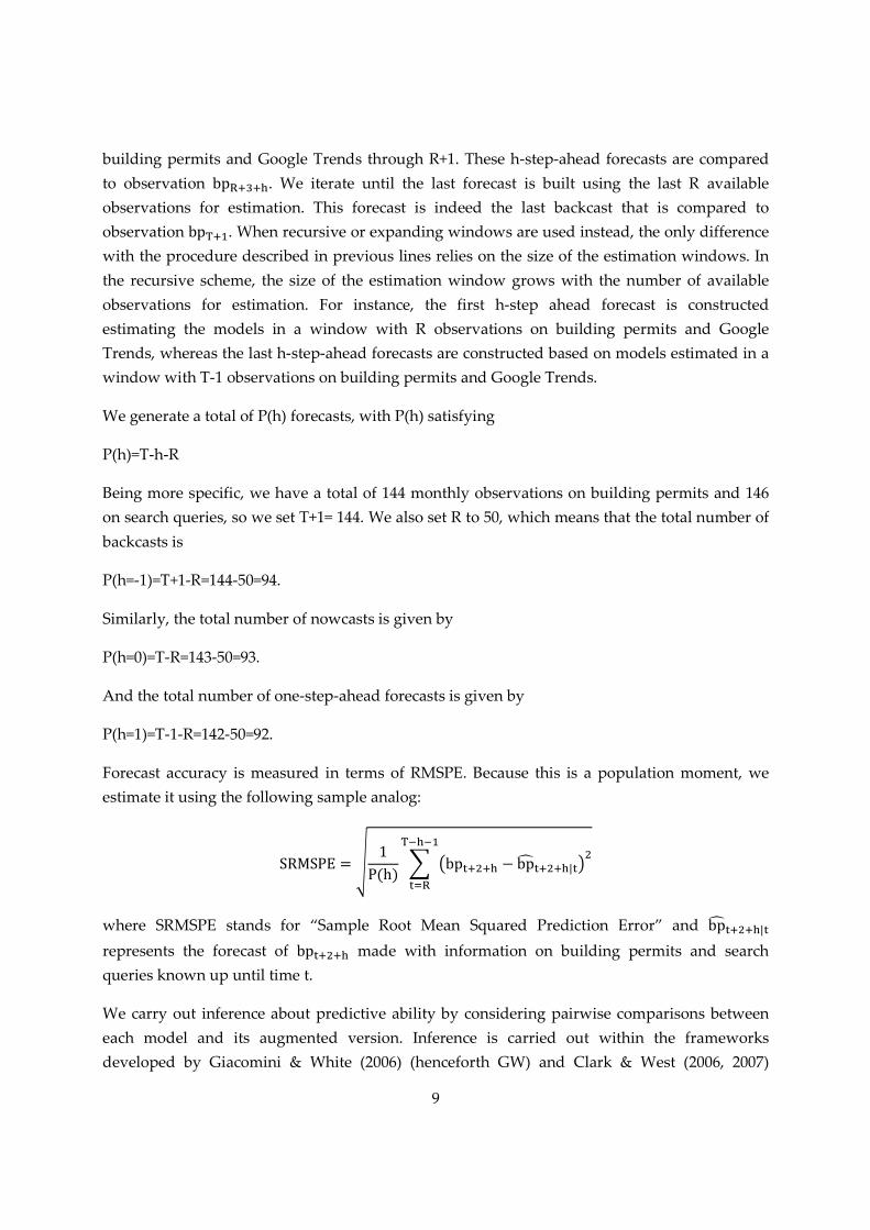
Forecast accuracy is measured in terms of RMSPE. Because this is a population moment, we

estimate it using the following sample analog:

SRMSPE = � 1P(h) � �bp�� − bp� ��|��

where SRMSPE stands for “Sample Root Mean Squared Prediction Error” and bp� ��|� represents the forecast of bp�� made with information on building permits and search

queries known up until time t.

We carry out inference about predictive ability by considering pairwise comparisons between

each model and its augmented version. Inference is carried out within the frameworks

developed by Giacomini & White (2006) (henceforth GW) and Clark & West (2006, 2007)

10

(henceforth CW). We focus on the unconditional version of the t-type statistic proposed by GW

which in practice coincides with the well-known test attributed to Diebold & Mariano (1995)

and West (1996) (henceforth DMW). This test has the distinctive feature of allowing

comparisons between two competing forecast methods instead of two competing models in a

given sample11.

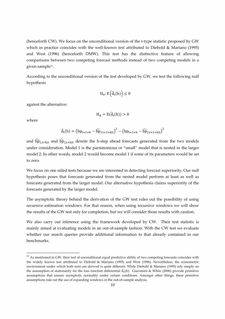
According to the unconditional version of the test developed by GW, we test the following null

hypothesis

H": E $d& �(h)' ≤ 0

against the alternative:

H* = E(d& �(h)) > 0

where

d& �(h) = �bp�� − bp�,��|�� − �bp�� − bp��,��|��

and bp�,��|� and bp��,��|� denote the h-step ahead forecasts generated from the two models

under consideration. Model 1 is the parsimonious or “small” model that is nested in the larger

model 2. In other words, model 2 would become model 1 if some of its parameters would be set

to zero.

We focus on one sided tests because we are interested in detecting forecast superiority. Our null

hypothesis poses that forecasts generated from the nested model perform at least as well as

forecasts generated from the larger model. Our alternative hypothesis claims superiority of the

forecasts generated by the larger model.

The asymptotic theory behind the derivation of the GW test rules out the possibility of using

recursive estimation windows. For that reason, when using recursive windows we will show

the results of the GW test only for completion, but we will consider those results with caution.

We also carry out inference using the framework developed by CW. Their test statistic is

mainly aimed at evaluating models in an out-of-sample fashion. With the CW test we evaluate

whether our search queries provide additional information to that already contained in our

benchmarks.

11

As mentioned in GW, their test of unconditional equal predictive ability of two competing forecasts coincides with

the widely known test attributed to Diebold & Mariano (1995) and West (1996). Nevertheless, the econometric

environment under which both tests are derived is quite different. While Diebold & Mariano (1995) rely simply on

the assumption of stationarity for the loss function differential d&�(h), Giacomini & White (2006) provide primitive

assumptions that ensure asymptotic normality under certain conditions. Amongst other things, these primitive

assumptions rule out the use of expanding windows in the out-of-sample analysis.

11

The CW test can be considered either as an encompassing test or as an adjusted comparison of

Mean Squared Prediction Errors (MSPE). The adjustment is made in order to make a fair

comparison between nested models. Intuitively, this test removes a term that introduces noise

when a parameter, that should be zero under the null hypothesis of equal MSPE, is estimated.

The core statistic of the CW test is constructed as follows

z-�� = �e-,�� − /�e-�,�� − �bp�,��|� − bp��,��|��0 Where e-,�� = bp�� − bp�,��|� and e-�,�� = bp�� − bp��,��|� represent the forecast

errors from the two models under consideration.

With some algebra it is straightforward to show that z-�� could also be expressed as follows

SMSPE − Adjusted = 2P(h) � e-,��e-,�� − e-�,�� (1)

This statistic is used to test the following null hypothesis

H": E(SMSPE − Adjusted) = 0

against the alternative

H*: E(SMSPE − Adjusted) > 0

CW suggest a one-sided test for a t-type statistic based upon the core statistic in (1). They

recommend asymptotically normal critical values for their test.

Three points are worth mentioning. First, it is important to emphasize that the CW test is fairly

different from either the test by GW or DMW. A key difference is that with the CW test we are

testing equal population forecasting ability under quadratic loss. In other words we are

evaluating the population difference in MSPE between two nested models. This is to be

distinguished from tests that focus on comparing the expected value of Sample Mean Squared

Prediction Errors between two forecasting methods. These tests, like GW, are not concerned

about comparing models, they are concerned about comparing forecasting performance in a

given sample.

Second, the CW test is not entirely new. In fact, the core statistic of the CW test is the same as

the core statistic of the encompassing test proposed by Harvey, Leybourne, & Newbold, (1998).

This implies that the CW test is also evaluating whether a particular combination between the

null and alternative model generates a forecasting strategy with the lowest RMSPE. The

novelty of CW compared to Harvey, Leybourne, & Newbold (1998) relies on the interpretation

12

of the test as a method to evaluate the difference in population MSPE between two nested

models, and on the fact that CW explicitly consider the role of parameter uncertainty.

Third, the asymptotic distribution of CW is analyzed in detail in Clark & McCracken (2001,

2005). In these papers the correct asymptotic distribution of the CW test is derived when one-

step-ahead forecasts are used (Clark & McCracken, 2001) and when longer horizon forecasts are

constructed via the direct method (Clark & McCracken, 2005). In the first paper it is shown that

the resulting asymptotic distribution of the CW test in general is not standard. In fact it is a

functional of Brownian motions depending on the number of excess parameters of the nesting

model, the limit of the ratio P(h)/R and the scheme used to update the estimates of the

parameters in the out-of-sample exercise. In the second paper Clark & McCracken (2005)

provide a generalization of their results for multistep ahead forecasts. Unfortunately, the

resulting asymptotic distribution of the CW statistic is again a functional of Brownian motions

but now depending on nuisance parameters. Differing from the previous work of Clark &

McCracken (2001, 2005), one of the key contributions of CW is to show via simulations that

normal critical values are indeed adequate in a variety of settings. They show that the cost of

approximating the correct critical values with standard normal critical values is in general low:

it produces a little undersized test. Further work by Clark & McCracken (2013) and Pincheira &

West (2016) show that normal critical values tend to work well when multistep ahead forecasts

are constructed using the iterative method, at least when the data generating process is not very

persistent. This is very important because in this paper we rely on the iterative method for the

construction of multistep ahead forecasts. We rely then on the vast simulations provided by

CW, Clark & McCracken (2013) and Pincheira & West (2016) to use standard normal critical

values in our out-of-sample exercises.

V. Forecasting Models

Our basic approach considers the comparison of forecasts coming from a benchmark model

with forecasts coming from the same benchmark but augmented with variables related to

specific search queries in Google Trends. We consider two main specifications that we describe

next:

∆ln(bp�) = α + <∆ln(bp��) + <�∆ln(bp��) + <�∆ln(bp��) + γ(L)?@+A@ (A.1)

?@ = B?@� + B�?@�� + C@ (A.2)

∆ln (bp�) = a + γ(L)?@+E@ (B.1)

(F − GH�)(F − IH − I�H�)E@ = J@ (B.2)

13

(F − KH�)(F − LH)?@ = M + N@ (B.3)

Where γ(L) = O"I + OH + O�H� represents a lag polynomial, L represents the lag operator such

that

HQR@ = R@�Q,

∆ represents the “difference operator” such that

∆R@ = R@ − R@�,

“I “ represents the identity operator, A@ , C@, E@, J@ and N@ correspond to white noise processes

and

?@ = ∆ST(U@) where zt denotes a generic search query in Google Trends. In other words, zt corresponds to

either the monthly time series on “real estate exam”, “new housing development”, “new

construction” or “new home construction”.

Our first specification is labeled specification A. It comprises expressions A.1 and A.2. Our

second specification is labeled B. It comprises expressions B.1, B.2 and B.3. We consider two

different specifications for robustness. We notice that specification A is linear, whereas

specification B is nonlinear.

For our in-sample analyses we consider both specifications (A and B). In these in-sample

analyses we are evaluating a contemporaneous relationship between building permits at time

t+1 and Google Trends search queries at time t+1 as well, so these in-sample analyses are not

predictive exercises necessarily, they are exercises aimed at determining a relationship between

building permits and Google Search queries that could potentially be used to obtained

backcasts, nowcasts and forecasts.

VI. Empirical Results

In-sample analysis

Tables 2-3 show diagnostic statistics associated to univariate versions of our specifications A

and B. Being more specific, Table 3 shows results of expression A.1 when γ(L) is set to zero, and

estimates of expression A.2 for each particular Google Search query. Similarly, Table 2 shows

results of expressions B.1 and B.2 when γ(L) is set to zero, and estimates of expression B.3 for

each particular Google Search query. We notice that estimates of the drift terms are removed

from Tables 2-3. A quick view of Tables 2-3 indicates that our specifications offer a decent

14

representation of the data as they are able to explain an important share of the total variation of

the respective dependent variable, most of the coefficients are statistically significant and the

Durbin-Watson statistic is close to 2 in most of the expressions.

Table 2: In-Sample Analysis: Basic nonlinear specifications.

Source: Own calculations based on US. Census and Google Trends data. * p<10%, ** p<5%, *** p<1%. HAC standard errors

according to Newey & West (1987) in parentheses. The operator dlog() refers to first log-difference monthly changes. Variables bp,

nhc, nc, nhd, rex refer to "building permits", "new home construction", "new construction","new housing development" and “real

estate exam”.

Table 3: In-Sample Analysis: Basic linear specifications.


according to Newey and West (1987) in parentheses. The operator ‘Lag’ refers to a lag in the dependent variable in months; dlog()

refers to first log-difference monthly changes. Variables bp, nhc, nc, nhd, rex refer to "building permits", "new home construction",

"new construction","new housing development" and “real estate exam”.

AR(1) -0.3366*** -0.2611*** -0.3208*** -03959*** -0.3574***

(0.0766) (0.0951) (0.0662) (0.0634) (0.0861)

AR(2) -0.1277*

(0.0761)

SAR(12) 0.7150*** 0.8668*** 0.3950*** 0.7918*** 0.6370***

(0.0793) (0.04623) (0.1005) (0.0523) (0.0794)

R-squared 0.4725 0.7806 0.2259 0.6132 0.4139

N 129 132 132 132 132

Durbin-Watson 1.9461 1.9336 2.1439 2.0376 2.0491

Schwarz criterion -1.7201 -3.3696 -1.3236 -2.2780 -1.7690

dlog(rex)Dependent Variable dlog(bp) dlog(nc) dlog(nhd) dlog(nhc)

Lag 1 -0.1896*** -0.0362 -0.2740*** -0.0857 -0.2017***

(0.0512) (0.0459) (0.0550) (0.0528) (0.0767)

Lag 2 0.1026

(0.0657)

Lag 12 0.6796*** 0.8509*** 0.3482*** 0.7310*** 0.5854***

(0.0653) (0.0511) (0.0937) (0.0689) (0.0872)

R-squared 0.4826 0.7591 0.2108 0.5534 0.3740

N 131 133 133 133 133

Durbin-Watson 2.1872 2.3913 2.1680 2.5718 2.2806

Schwarz criterion -1.6904 -3.2444 -1.2753 -2.1055 -1.6743

Dependent Variable dlog(bp) dlog(nc) dlog(nhd) dlog(nhc) dlog(rex)

15

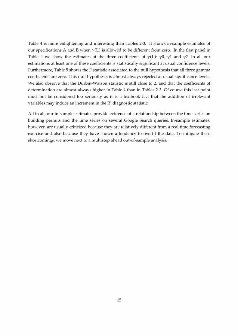
Table 4 is more enlightening and interesting than Tables 2-3. It shows in-sample estimates of

our specifications A and B when γ(L) is allowed to be different from zero. In the first panel in

Table 4 we show the estimates of the three coefficients of γ(L): γ0, γ1 and γ2. In all our

estimations at least one of these coefficients is statistically significant at usual confidence levels.

Furthermore, Table 5 shows the F statistic associated to the null hypothesis that all three gamma

coefficients are zero. This null hypothesis is almost always rejected at usual significance levels.

We also observe that the Durbin-Watson statistic is still close to 2, and that the coefficients of

determination are almost always higher in Table 4 than in Tables 2-3. Of course this last point

must not be considered too seriously as it is a textbook fact that the addition of irrelevant

variables may induce an increment in the R2 diagnostic statistic.

All in all, our in-sample estimates provide evidence of a relationship between the time series on

building permits and the time series on several Google Search queries. In-sample estimates,

however, are usually criticized because they are relatively different from a real time forecasting

exercise and also because they have shown a tendency to overfit the data. To mitigate these

shortcomings, we move next to a multistep ahead out-of-sample analysis.

16

Table 4: In-Sample Analysis: Explaining Building Permits with Google Trends


according to Newey and West (1987) in parentheses. The dependent variable is the monthly log-difference in building permits. The

operator dlog() refers to log-difference monthly changes. Variables bp, nhc, nc, nhd and rex refer to "building permits", "new home

construction", "new construction", "new housing development" and “real estate exam”.

dlog(nhc) 0.0987 0.0562

(0.0910) (0.0636)

dlog(nhc(-1)) 0.284*** 0.0824

(0.1073) (0.0657)

dlog(nhc(-2)) 0.4088*** 0.2425**

(0.1197) (0.1066)

dlog(nc) 0.2124 0.1361

(0.1593) (0.0957)

dlog(nc(-1)) 0.2473 0.1139

(0.1752) (0.0728)

dlog(nc(-2)) 0.7389*** 0.4520***

(0.1122) (0.0902)

dlog(nhd) 0.0431 0.0817

(0.0611) (0.0609)

dlog(nhd(-1)) 0.0556 0.1004

(0.0573) (0.0628)

dlog(nhd(-2)) 0.1091* 0.1609***

(0.0578) (0.0639)

dlog(rex) -0.0547 0.0248

(0.0977) (0.072)

dlog(rex(-1)) 0.2400*** 0.1788**

0.084539 (0.0748)

dlog(rex(-2)) 0.1866** 0.2223***

(0.0865) (0.0758)

AR(1) -0.4898*** -0.4625*** -0.3497*** -0.3701***

(0.0648) (0.0700) (0.0806) (0.0815)

AR(2) -0.2539*** -0.1969** -0.1374* -0.1767**

(0.0851) (0.0787) (0.0762) (0.0747)

SAR(12) 0.5746*** 0.4871*** 0.6669*** 0.6385***

(0.0897) (0.0824) (0.0857) (0.0679)

dlog(bp(-1)) -0.2104*** -0.2463*** -0.2167*** -0.2416***

(0.0512) (0.0491) (0.0515) (0.0483)

dlog(bp(-2)) 0.0964 0.0897 0.0905 0.0634

(0.063) (0.0645) (0.0731) (0.0618)

dlog(bp(-12)) 0.5430*** 0.4901*** 0.6016*** 0.5655***

(0.0648) (0.0619) (0.0673) (0.0629)

R-squared 0.5483 0.557 0.482 0.511 0.518 0.552 0.504 0.527

N 127 127 127 127 131 131 131 131

Durbin-Watson 1.964 1.971 1.944 1.955 2.347 2.276 2.218 2.248

F-statistic 24.273 25.189 18.576 20.868 22.226 25.437 21.040 22.987

P-value 0.000 0.000 0.000 0.000 0.000 0.000 0.000 0.000

Schwarz criterion -1.706 -1.726 -1.568 -1.626 -1.650 -1.722 -1.622 -1.668

(6) (7) (8)Dep. Var.: dlog(bp) (1) (2) (3) (4) (5)

17

Table 5: In-Sample Analysis: Joint significance of Google Search Queries

Source: Own calculations based on US. Census and Google Trends data. HAC standard errors according to Newey and West (1987)

are used in the construction of the tests. The null hypothesis is that the parameters associated to the search queries

(contemporaneous and the first two lags) are all jointly equal to zero. For specifications (1) and (5) the search queries are "nhc"; for

(2) and (6), "nc"; for (3) and (7), "nhd"; and for (4) and (8), "rex". Variables nhc, nc, nhd and rex refer to "new home construction",

"new construction","new housing development" and "real estate exam", respectively.

Out-of-sample analysis

Table 6-13 show results of our out-of-sample exercises. In particular, Tables 6-9 show the CW

core statistic, its standard errors and the corresponding t-statistics. Tables 10-13 show similar

results but for the GW/DMW test.

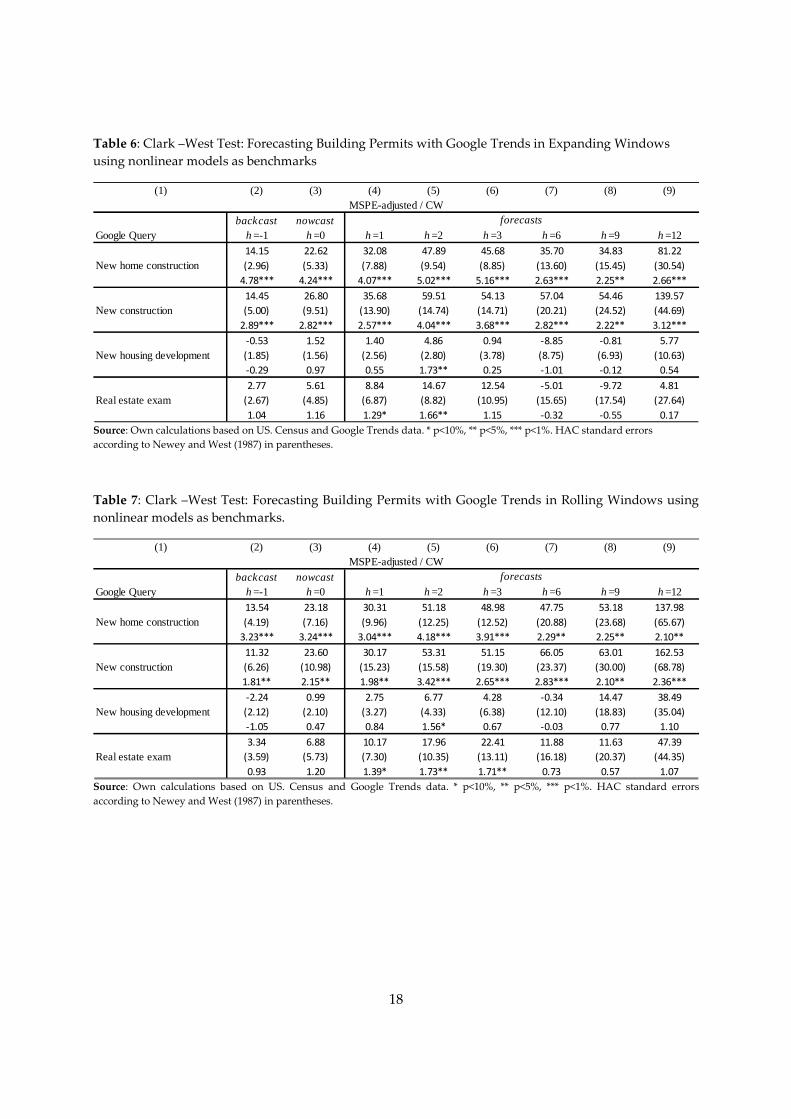
Table 6-13 show strong evidence of predictability for two Google Search queries: “new home

construction” and “new construction”. This predictability is robust to our model specifications

(linear or nonlinear), to the use of expanding or rolling windows, and also to the forecasting

horizon. In particular, our results indicate that these two search queries are useful for

backcasting, nowcasting and forecasting building permits in the U.S. Furthermore, in most

cases evidence of predictability is found at extremely tight significance levels: 5% or even 1% in

many cases.

For the other two search queries under analysis, our results are slightly less compelling. We do

find evidence of predictability, but this evidence is not always robust to different forecasting

horizons, model specifications and to the use of expanding or rolling windows. Robust results

are found for both search queries when predicting building permits two months ahead and also

for the query “real state exam” when forecasting one month ahead. At other forecasting

horizons we obtain mixed results. This means little evidence of predictability in our nonlinear

specifications but stronger evidence when using our linear specifications. Interestingly, for the

search query “real state exam” the general picture is a little better than in the case of “new

housing development”.

Wald Test (Chi-square) 26.530 54.356 5.443 17.511 8.099 27.641 9.833 12.856

P-value 0.000 0.000 0.142 0.001 0.044 0.000 0.020 0.005

F- Test 8.843 18.119 1.814 5.837 2.700 9.214 3.278 4.285

P-value 0.000 0.000 0.148 0.001 0.049 0.000 0.023 0.007

(5) (6) (7) (8)Model Specification (1) (2) (3) (4)

18

Table 6: Clark –West Test: Forecasting Building Permits with Google Trends in Expanding Windows

using nonlinear models as benchmarks


according to Newey and West (1987) in parentheses.

Table 7: Clark –West Test: Forecasting Building Permits with Google Trends in Rolling Windows using

nonlinear models as benchmarks.



(1) (2) (3) (4) (5) (6) (7) (8) (9)

backcast nowcastGoogle Query h =-1 h =0 h =1 h =2 h =3 h =6 h =9 h =12

14.15 22.62 32.08 47.89 45.68 35.70 34.83 81.22

New home construction (2.96) (5.33) (7.88) (9.54) (8.85) (13.60) (15.45) (30.54)

4.78*** 4.24*** 4.07*** 5.02*** 5.16*** 2.63*** 2.25** 2.66***

14.45 26.80 35.68 59.51 54.13 57.04 54.46 139.57

New construction (5.00) (9.51) (13.90) (14.74) (14.71) (20.21) (24.52) (44.69)

2.89*** 2.82*** 2.57*** 4.04*** 3.68*** 2.82*** 2.22** 3.12***

-0.53 1.52 1.40 4.86 0.94 -8.85 -0.81 5.77

New housing development (1.85) (1.56) (2.56) (2.80) (3.78) (8.75) (6.93) (10.63)

-0.29 0.97 0.55 1.73** 0.25 -1.01 -0.12 0.54

2.77 5.61 8.84 14.67 12.54 -5.01 -9.72 4.81

Real estate exam (2.67) (4.85) (6.87) (8.82) (10.95) (15.65) (17.54) (27.64)

1.04 1.16 1.29* 1.66** 1.15 -0.32 -0.55 0.17

MSPE-adjusted / CWforecasts

(1) (2) (3) (4) (5) (6) (7) (8) (9)


13.54 23.18 30.31 51.18 48.98 47.75 53.18 137.98


3.23*** 3.24*** 3.04*** 4.18*** 3.91*** 2.29** 2.25** 2.10**

11.32 23.60 30.17 53.31 51.15 66.05 63.01 162.53


1.81** 2.15** 1.98** 3.42*** 2.65*** 2.83*** 2.10** 2.36***

-2.24 0.99 2.75 6.77 4.28 -0.34 14.47 38.49


-1.05 0.47 0.84 1.56* 0.67 -0.03 0.77 1.10

3.34 6.88 10.17 17.96 22.41 11.88 11.63 47.39

Real estate exam (3.59) (5.73) (7.30) (10.35) (13.11) (16.18) (20.37) (44.35)

0.93 1.20 1.39* 1.73** 1.71** 0.73 0.57 1.07


19

Table 8: Clark –West Test: Forecasting Building Permits with Google Trends in Expanding Windows,

using Linear Models as benchmarks



Table 9: Clark –West Test: Forecasting Building Permits with Google Trends in Rolling Windows, using

Linear Models as benchmarks



Tables 10-13 show sample Root Mean Squared Prediction Errors (RMSPE) and the t-statistics of

the GW/DMW test. We notice that we expect weaker results using the GW/DMW test because

our analysis involves the forecasting ability of two models, one nested in the other. Let us recall

that in nested environments the CW test removes a term that should be zero in population

under the null hypothesis, but that is not zero in finite samples. Tables 10-13 corroborate this

prior as the corresponding t-statistics of the GW/DMW test are always lower than the t-statistics

of the CW test, comparing the same forecasting exercises, of course. Despite this regularity,

Tables 10-13 still provide evidence of predictability in some cases. The most robust evidence is

(1) (2) (3) (4) (5) (6) (7) (8) (9)


4.60 11.83 25.10 38.27 42.07 30.15 13.05 39.18


2.62*** 3.12*** 3.45*** 4.37*** 4.34*** 3.13*** 1.34** 2.02**

11.96 21.02 29.71 53.80 49.66 41.51 28.10 96.26


3.46*** 3.26*** 2.96*** 4.93*** 5.06*** 3.34*** 1.71** 3.28***

2.78 7.94 12.68 23.57 17.87 -0.48 0.36 26.91


1.53* 2.96*** 2.81*** 3.12*** 2.19** -0.06 0.05 1.73**

6.65 14.76 25.74 42.85 42.95 25.96 20.82 72.69

Real Estate Exam (2.28) (4.85) (7.36) (8.63) (10.34) (16.06) (17.60) (33.98)

2.91*** 3.04*** 3.50*** 4.97*** 4.15*** 1.62* 1.18 2.14**


(1) (2) (3) (4) (5) (6) (7) (8) (9)


4.35 12.02 23.02 36.69 41.02 29.15 7.14 32.10


1.83** 2.87*** 2.99*** 4.17*** 4.47*** 2.35*** 0.49 0.92

10.86 21.67 30.86 53.04 50.88 41.30 13.11 77.14


2.97*** 2.96*** 2.90*** 4.90*** 5.60*** 2.70*** 0.60 1.60*

2.22 8.21 17.23 30.69 24.07 -0.51 -4.26 38.48


0.83 2.11** 3.18*** 3.30*** 2.45*** -0.05 -0.27 1.10

8.61 19.02 25.31 44.30 45.78 34.42 29.06 99.73

Real Estate Exam (3.51) (6.10) (8.09) (9.63) (13.87) (18.29) (22.09) (52.11)

2.45*** 3.12*** 3.13*** 4.60*** 3.30*** 1.88** 1.32* 1.91**


20

found for the query: “new home construction” for which we do find evidence of

“nowcastability” in all our forecasting exercises, for instance. Evidence of predictability with the

GW/DMW test may also be found for the rest of the queries under analysis, more so when

forecasting at short horizons, although this evidence is not always robust across our different

out-of-sample exercises.

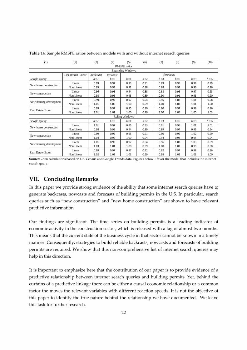
It is also interesting to mention some results regarding forecast accuracy. In the last row of

Tables 10-13 we show sample RMSPE of our benchmark models. This is a measure of forecast

accuracy when our models generate forecasts without the information provided by Google

Trends. It is straightforward to compare this baseline sample RMSPE with that reported for

each search query. Simple algebra leads to show that the most important gains in forecast

accuracy are obtained using the query “new home construction” and “new construction”. These

queries allow gains of more than 10% in sample RMSPE when forecasting two and three

months ahead. Table 14 provides a summary of these sample RMSPE ratios.

It is also important to mention that the lowest sample RMSPE across all our forecasting

exercises is achieved when using our nonlinear models with expanding estimation windows

(see Table 10). At short horizons the lowest sample RMSPE is achieved when our nonlinear

specification is augmented with “new home construction”, and at longer horizons of 6, 9 and 12

months ahead, the lowest sample RMSPE is achieved when our nonlinear specification is

augmented with the query “new construction”.

In summary, we find relatively strong evidence of predictability for our supply side queries

“new home construction” and “new construction”, and slightly less compelling evidence for the

queries “new housing development” and “real state exam”.

Table 10: Diebold-Mariano-West Test: Forecasting Building Permits with Google Trends in Expanding

Windows, using Nonlinear Models as benchmarks



(1) (2) (3) (4) (5) (6) (7) (8) (9) (10)

RMSPE/DMW backcast nowcastGoogle Query h =-1 h =0 h =1 h =2 h =3 h =6 h =9 h =12

RMSPE 7.74 8.74 9.37 10.31 10.46 12.62 14.53 18.05

DMW 2.57*** 2.23** 2.64*** 3.91*** 4.10*** 1.42* 1.21 0.98

RMSPE 7.98 8.84 9.72 10.44 10.65 12.22 14.15 17.05

DMW 0.60 0.91 0.77 2.14** 2.02** 1.51* 1.21 1.35*

RMSPE 8.26 9.31 10.25 11.62 11.93 13.86 15.33 18.90

DMW -0.75 0.32 0.02 1.07 -0.37 -1.38 -0.77 -0.04

RMSPE 8.24 9.41 10.28 11.58 11.82 14.06 15.92 19.47

DMW -0.45 -0.32 -0.09 0.54 0.13 -1.18 -1.34 -0.94

RMSPE benchmark 8.17 9.33 10.25 11.75 11.88 13.39 15.16 18.89

Real estate exam

RMSPE and DMW testforecasts

New home construction

New construction

New housing development

21

Table 11: Diebold-Mariano-West Test: Forecasting Building Permits with Google Trends in Rolling

Windows, using Nonlinear Models as benchmarks



Table 12: Diebold-Mariano-West Test: Forecasting Building Permits with Google Trends in Expanding

Windows, using Linear Models as benchmarks



Table 13: Diebold-Mariano-West Test: Forecasting Building Permits with Google Trends in Rolling

Windows, using Linear Models as benchmarks

Source: Own calculations based on US. Census and Google Trends data. * p<10%, ** p<5%, *** p<1%. DMW t statistic is calculated

using HAC standard errors according to Newey and West (1987).

(1) (2) (3) (4) (5) (6) (7) (8) (9) (10)


RMSPE 8.15 9.05 9.74 10.54 10.90 13.50 16.29 21.09

DMW 0.67 1.33* 1.49* 2.97*** 2.85*** 1.18 1.18 0.89

RMSPE 8.68 9.41 10.38 11.17 11.49 13.30 16.34 21.05

DMW -0.66 0.13 -0.01 1.03 0.93 1.22 0.87 0.84

RMSPE 8.59 9.60 10.40 11.77 12.25 14.68 17.02 21.97

DMW -1.99 -1.00 -0.18 0.61 -0.12 -0.78 0.26 0.63

RMSPE 8.48 9.67 10.46 11.71 11.93 14.61 17.35 22.34

DMW -0.88 -0.74 -0.31 0.48 0.75 -0.49 -0.38 0.12

RMSPE benchmark 8.31 9.49 10.37 11.87 12.22 14.37 17.15 22.43

Real estate exam



New construction


(1) (2) (3) (4) (5) (6) (7) (8) (9) (10)


RMSPE 8.24 9.47 10.29 11.69 11.32 13.01 14.75 18.57

DMW 1.02 1.84** 2.58*** 3.70*** 3.86*** 2.12** 0.49 0.46

RMSPE 8.05 9.16 10.35 11.30 11.21 12.81 14.46 17.48

DMW 1.61* 2.04** 1.68** 3.92*** 4.16*** 2.29** 0.90 1.72**

RMSPE 8.30 9.50 10.67 12.10 12.18 13.97 15.10 18.41

DMW 0.45 2.35*** 2.15** 2.78*** 1.77** -0.76 -0.73 1.05

RMSPE 8.23 9.49 10.45 11.64 11.42 13.40 14.71 18.02

DMW 0.91 1.19 1.73** 3.68*** 3.45*** 0.61 0.34 0.91

RMSPE benchmark 8.35 9.81 11.05 12.86 12.71 13.76 14.92 18.83



New construction


Real Estate Exam

(1) (2) (3) (4) (5) (6) (7) (8) (9) (10)


RMSPE 8.48 9.74 10.93 12.42 12.15 13.92 16.44 21.44

DMW -0.58 1.46* 1.71** 3.11*** 3.76*** 1.21 -0.39 -0.18

RMSPE 8.34 9.51 10.89 12.13 12.01 13.84 16.48 21.11

DMW 0.22 1.55* 1.41* 3.40*** 4.08*** 1.08 -0.36 0.11

RMSPE 8.51 9.88 11.08 12.53 12.76 14.95 16.79 21.15

DMW -0.74 0.74 2.03** 2.68*** 1.71** -1.33 -1.17 0.13

RMSPE 8.34 9.70 11.09 12.38 12.24 14.12 15.96 20.35

DMW 0.24 1.12 1.09 3.05*** 2.46*** 0.63 0.40 0.85

RMSPE benchmark 8.38 10.02 11.47 13.39 13.34 14.50 16.23 21.26


Real Estate Exam



New construction

22

Table 14: Sample RMSPE ratios between models with and without internet search queries

Source: Own calculations based on US. Census and Google Trends data. Figures below 1 favor the model that includes the internet

search query.

VII. Concluding Remarks

In this paper we provide strong evidence of the ability that some internet search queries have to

generate backcasts, nowcasts and forecasts of building permits in the U.S. In particular, search

queries such as “new construction” and “new home construction” are shown to have relevant

predictive information.

Our findings are significant. The time series on building permits is a leading indicator of

economic activity in the construction sector, which is released with a lag of almost two months.

This means that the current state of the business cycle in that sector cannot be known in a timely

manner. Consequently, strategies to build reliable backcasts, nowcasts and forecasts of building

permits are required. We show that this non-comprehensive list of internet search queries may

help in this direction.

It is important to emphasize here that the contribution of our paper is to provide evidence of a

predictive relationship between internet search queries and building permits. Yet, behind the

curtains of a predictive linkage there can be either a causal economic relationship or a common

factor the moves the relevant variables with different reaction speeds. It is not the objective of

this paper to identify the true nature behind the relationship we have documented. We leave

this task for further research.

(1) (2) (3) (4) (5) (6) (7) (8) (9) (10)

Linear/Non Linear backcast nowcastGoogle Query h =-1 h =0 h =1 h =2 h =3 h =6 h =9 h =12

Linear 0.99 0.97 0.93 0.91 0.89 0.95 0.99 0.99

Non Linear 0.95 0.94 0.91 0.88 0.88 0.94 0.96 0.96

Linear 0.96 0.93 0.94 0.88 0.88 0.93 0.97 0.93

Non Linear 0.98 0.95 0.95 0.89 0.90 0.91 0.93 0.90

Linear 0.99 0.97 0.97 0.94 0.96 1.02 1.01 0.98

Non Linear 1.01 1.00 1.00 0.99 1.00 1.03 1.01 1.00

Linear 0.99 0.97 0.95 0.90 0.90 0.97 0.99 0.96

Non Linear 1.01 1.01 1.00 0.99 1.00 1.05 1.05 1.03

Google Query h =-1 h =0 h =1 h =2 h =3 h =6 h =9 h =12Linear 1.01 0.97 0.95 0.93 0.91 0.96 1.01 1.01

Non Linear 0.98 0.95 0.94 0.89 0.89 0.94 0.95 0.94

Linear 0.99 0.95 0.95 0.91 0.90 0.95 1.02 0.99

Non Linear 1.04 0.99 1.00 0.94 0.94 0.93 0.95 0.94

Linear 1.01 0.99 0.97 0.94 0.96 1.03 1.03 0.99

Non Linear 1.03 1.01 1.00 0.99 1.00 1.02 0.99 0.98

Linear 0.99 0.97 0.97 0.92 0.92 0.97 0.98 0.96

Non Linear 1.02 1.02 1.01 0.99 0.98 1.02 1.01 1.00

Real Estate Exam

Expanding WindowsRMSPE ratios

forecasts


New construction


Rolling Windows


New construction


Real Estate Exam

23

Our paper is part of a large literature that in the recent years has evaluated the predictive

usefulness of the information that is available on the web. This is an attractive line of research

because of the large and increasing proportion of internet users, the high frequency of the data

that is released by Google Trends and the relative speed with which this data is released to the

public.

A natural avenue of future research considers the evaluation of the predictive ability of our

preferred search queries when forecasting measures of economic activity in more complex

economic models. Similarly, we only have explored the predictive ability of simple internet

search queries, without considering forecast combinations or more advanced techniques of

dimensionality reduction. This also seems to be another attractive line of future research.

References

Aruoba, S. B., & Diebold, F. X. (2010). Real-Time Macroeconomic Monitoring: Real Activity, Inflation, and

Interactions. American Economic Review, 100(2), 20–24. http://doi.org/10.1257/aer.100.2.20

Askitas, N. (2015). Trend-Spotting in the Housing Market (IZA Discussion Paper No. 9427). Retrieved from

http://papers.ssrn.com/abstract=2675484

Askitas, N., & Zimmermann, K. (2009). Google Econometrics and Unemployment Forecasting.

Askitas, N., & Zimmermann, K. F. (2011). Detecting Mortgage Delinquencies with Google Trends. IZA

Discussion Paper 5895.

Beracha, E., & Wintoki, M. B. (2013). Forecasting residential real estate price changes from online search

activity. Journal of Real Estate Research, 35(3), 283–312.

Bollen, J., Mao, H., & Zeng, X. (2011). Twitter mood predicts the stock market. Journal of Computational

Science, 2(1), 1–8. Retrieved from

http://www.sciencedirect.com/science/article/pii/S187775031100007X

Bordino, I., Battiston, S., Caldarelli, G., Cristelli, M., Ukkonen, A., & Weber, I. (2012). Web search queries

can predict stock market volumes. PloS One, 7(7), e40014. Retrieved from

http://journals.plos.org/plosone/article?id=10.1371/journal.pone.0040014

Carrière-Swallow, Y., & Labbé, F. (2013). Nowcasting with Google Trends in an Emerging Market. Journal

of Forecasting, 32(4), 289–298. http://doi.org/10.1002/for.1252

Chauvet, M., Gabriel, S., & Lutz, C. (2016). Mortgage default risk: New evidence from internet search

queries. Journal of Urban Economics, 96(November), 91–111. Retrieved from

http://dx.doi.org/10.1016/j.jue.2016.08.004

Chen, S.-S. (2009). Predicting the bear stock market: Macroeconomic variables as leading indicators.

Journal of Banking & Finance, 33(2), 211–223. http://doi.org/10.1016/j.jbankfin.2008.07.013

Choi, H., & Varian, H. (2012). Predicting the Present with Google Trends. Economic Record, 88(SUPPL.1),

2–9. http://doi.org/10.1111/j.1475-4932.2012.00809.x

Clark, T. E., & McCracken, M. W. (2001). Tests of equal forecast accuracy and encompassing for nested

24

models. Journal of Econometrics, 105(1), 85–110. http://doi.org/10.1016/S0304-4076(01)00071-9

Clark, T. E., & McCracken, M. W. (2005). Evaluating Direct Multistep Forecasts. Econometric Reviews,

24(4), 369–404. http://doi.org/10.1080/07474930500405683

Clark, T. E., & McCracken, M. W. (2013). Evaluating the Accuracy of Forecasts from Vector

Autoregressions. In T. Fomby, L. Killian, & A. Murphy (Eds.), Vector Autoregressive Modeling—New

Developments and Applications: Essays in Honor of Christopher A. Sims.

Clark, T. E., & West, K. D. (2007). Approximately normal tests for equal predictive accuracy in nested

models. Journal of Econometrics, 138(1), 291–311. http://doi.org/10.1016/j.jeconom.2006.05.023

D’Amuri, F., & Marcucci, J. (2012). The predictive power of Google searches in forecasting unemployment (Bank

of Italy Working Paper No. 891).

Da, Z., Engelberg, J., & Gao, P. (2015). The Sum of All FEARS Investor Sentiment and Asset Prices. Review

of Financial Studies, 28(1), 1–32. http://doi.org/10.1093/rfs/hhu072

DA, Z., ENGELBERG, J., & GAO, P. (2011). In Search of Attention. The Journal of Finance, 66(5), 1461–1499.

http://doi.org/10.1111/j.1540-6261.2011.01679.x

Das, P., Ziobrowski, A., & Coulson, N. E. (2015). Online Information Search, Market Fundamentals and

Apartment Real Estate. The Journal of Real Estate Finance and Economics, 51(4), 480–502. Retrieved

from http://link.springer.com/10.1007/s11146-015-9496-1

Diebold, F. X., & Mariano, R. S. (1995). Comparing Predictive Accuracy. Journal of Business & Economic

Statistics, 13(3), 253–263. http://doi.org/10.1080/07350015.1995.10524599

Dimpfl, T., & Jank, S. (2016). Can Internet Search Queries Help to Predict Stock Market Volatility?

European Financial Management, 22(2), 171–192. http://doi.org/10.1111/eufm.12058

Dzielinski, M. (2012). Measuring economic uncertainty and its impact on the stock market. Finance

Research Letters, 9(3), 167–175. http://doi.org/10.1016/j.frl.2011.10.003

Estrella, A., & Mishkin, F. S. (1998). Predicting U.S. Recessions: Financial Variables as Leading Indicators.

Review of Economics and Statistics, 80(1), 45–61. http://doi.org/10.1162/003465398557320

Giacomini, R., & White, H. (2006). Tests of Conditional Predictive Ability. Econometrica, 74(6), 1545–1578.

http://doi.org/10.1111/j.1468-0262.2006.00718.x

Giannone, D., Reichlin, L., & Small, D. (2008). Nowcasting: The real-time informational content of

macroeconomic data. Journal of Monetary Economics, 55(4), 665–676.

http://doi.org/10.1016/j.jmoneco.2008.05.010

Guzmán, G. (2011, January 1). Internet search behavior as an economic forecasting tool: The case of

inflation expectations. Journal of Economic and Social Measurement. IOS Press.

http://doi.org/10.3233/JEM-2011-0342

Harvey, D. S., Leybourne, S. J., & Newbold, P. (1998). Tests for Forecast Encompassing. Journal of Business

& Economic Statistics, 16(2), 254–259. http://doi.org/10.1080/07350015.1998.10524759

Huberty, M. (2015). Can we vote with our tweet? On the perennial difficulty of election forecasting with

social media. International Journal of Forecasting, 31(3), 992–1007.

http://doi.org/10.1016/j.ijforecast.2014.08.005

Joseph, K., Babajide Wintoki, M., & Zhang, Z. (2011). Forecasting abnormal stock returns and trading

volume using investor sentiment: Evidence from online search. International Journal of Forecasting,

27(4), 1116–1127. http://doi.org/10.1016/j.ijforecast.2010.11.001

Kearney, M. S., & Levine, P. B. (2015). Media Influences on Social Outcomes: The Impact of MTV’s 16 and

25

Pregnant on Teen Childbearing †. American Economic Review, 105(12), 3597–3632. Retrieved from

https://www.aeaweb.org/articles?id=10.1257/aer.20140012

Kristoufek, L. (2013). Can Google Trends search queries contribute to risk diversification? Scientific

Reports, 3, 2713. http://doi.org/10.1038/srep02713

McLaren, N., & Shanbhogue, R. (2011). Using Internet Search Data as Economic Indicators. Bank of

England Quarterly Bulletin, Q2(June 13, 2011).

Moat, H. S., Curme, C., Avakian, A., Kenett, D. Y., Stanley, H. E., & Preis, T. (2013). Quantifying

Wikipedia Usage Patterns Before Stock Market Moves. Scientific Reports, 3, 1801. Retrieved from

http://www.nature.com/srep/2013/130508/srep01801/full/srep01801.html

Newey, W., & West, K. (1987). A simple, positive semi-definite, heteroskedasticity and

autocorrelationconsistent covariance matrix. Econometrica, 55(3), 703–708.

http://doi.org/10.3386/t0055

Oestmann, M., & Bennöhr, L. (2015). Determinants of house price dynamics. What can we learn from search

engine data? (No. A15-V3). Beiträge zur Jahrestagung des Vereins für Socialpolitik. Retrieved from

https://www.econstor.eu/dspace/bitstream/10419/113198/1/VfS_2015_pid_849.pdf

Pincheira, P. M., & West, K. D. (2016). A comparison of some out-of-sample tests of predictability in

iterated multi-step-ahead forecasts. Research in Economics, 70(2), 304–319.

http://doi.org/10.1016/j.rie.2016.03.002

Preis, T., Reith, D., & Stanley, H. E. (2010). Complex dynamics of our economic life on different scales:

insights from search engine query data. Philosophical Transactions. Series A, Mathematical, Physical, and

Engineering Sciences, 368(1933), 5707–19. Retrieved from

http://rsta.royalsocietypublishing.org/content/368/1933/5707.abstract

Ripberger, J. T. (2011). Capturing Curiosity: Using Internet Search Trends to Measure Public

Attentiveness. Policy Studies Journal, 39(2), 239–259. http://doi.org/10.1111/j.1541-0072.2011.00406.x

Smith, G. P. (2012). Google Internet search activity and volatility prediction in the market for foreign

currency. Finance Research Letters, 9(2), 103–110. http://doi.org/10.1016/j.frl.2012.03.003

Smith, P. (2016). Google’s MIDAS Touch: Predicting UK Unemployment with Internet Search Data.

Journal of Forecasting, n/a-n/a. http://doi.org/10.1002/for.2391

Strauss, J. (2013). Does housing drive state-level job growth? Building permits and consumer expectations

forecast a state’s economic activity. Journal of Urban Economics, 73(1), 77–93.

http://doi.org/10.1016/j.jue.2012.07.005

Tefft, N. (2011). Insights on unemployment, unemployment insurance, and mental health. Journal of

Health Economics, 30(2), 258–64. http://doi.org/10.1016/j.jhealeco.2011.01.006

Vlastakis, N., & Markellos, R. N. (2012). Information demand and stock market volatility. Journal of

Banking & Finance, 36(6), 1808–1821. http://doi.org/10.1016/j.jbankfin.2012.02.007

Vosen, S., & Schmidt, T. (2011). Forecasting private consumption: survey-based indicators vs. Google

trends. Journal of Forecasting, 30(6), 565–578. http://doi.org/10.1002/for.1213

West, K. D. (1996). Asymptotic Inference about Predictive Ability. Econometrica, 64(5), 1067–1084.

Retrieved from www.jstor.org/stable/2171956

Wu, L., & Brynjolfsson, E. (2015). The Future of Prediction: How Google Searches Foreshadow Housing

Prices and Sales. In Economic Analysis of the Digital Economy (pp. 89–118).

26

Appendix

Figure A1: Autocorrelograms in First Log-Differences.

Source: Own calculations based on US. Census and Google Trends data.

Figure A2: Cross Correlograms of Building Permits and Google Search Queries (levels).


27

Figure A3: Cross Correlograms of Building Permits and Google Search Queries (first differences).


Table A1: Unit Root Tests

Source: Own calculations based on US. Census and Google Trends data. * p<10%, ** p<5%, *** p<1%. The null hypotheses of both

tests indicate the existence of a unit root. The levels are natural logarithms of the raw series, and the first difference is their monthly

log-difference.

Building Permits Real Estate ExamNew Housing

DevelopmentNew Construction

New Home

Construction

Levels

Standard -1.766 -1.924 -2.281 -2.169 -2.063

With trend -1.736 -1.636 -3.288* -2.476 -2.079

With drift -1.766** -1.924** -2.281** -2.169** -2.063**

First differences

Standard -13.895*** -13.611*** -15.483*** -12.682*** -12.073***

With trend -13.884*** -13.678*** -15.491*** -12.676*** -12.105***

With drift -13.895*** -13.611*** -15.483*** -12.682*** -12.073***

Levels

Standard -1.733 -1.779 -2.136 -1.976 -1.929

With trend -1.713 -1.366 -2.817 -2.216 -1.794

First differences

Standard -13.784*** -13.776*** -17.156*** -12.970*** -12.313***

With trend -13.783*** -13.903*** -17.287*** -12.983*** -12.385***

Augmented Dickey-Fuller Test

Phillips-Perron Test

nowcasting building permits with google trends · 0 3 5 $ munich personal repec archive nowcasting...

Documents