npt’s mobile cost model version 7
TRANSCRIPT

Report for the Norwegian Post and
Telecommunications Authority
NPT’s mobile cost model version 7.1
Model documentation
PUBLIC VERSION
24 August 2010
Ref: 16928-315a
Ref: 16928-315a
Contents
1 Introduction 1
2 Installing and running the model 3
2.1 Running the model 3
2.2 Model worksheets 3
2.3 Description and location of main inputs 5
3 Demand assumptions 7
3.1 Market demand 7
3.2 Market share 9
4 Network assumptions 11
4.1 Radio network 11
4.2 Core network 21
4.3 Other network elements 26
4.4 Non-network elements 26
4.5 Third operator 27
4.6 MVNO networks 27
5 Expenditure calculations 29
5.1 Purchasing, replacement and capex planning period 29
5.2 Network closure 29
5.3 MEA equipment unit price 30
5.4 Phase 1 distribution of expenditures for Telenor and NetCom 30
6 Annualisation of expenditure 31
6.1 Rationale for using economic depreciation 31
6.2 Implementation of economic depreciation principles 32
6.3 Implementation of the economic depreciation algorithm 34
6.4 Implementation of HCA depreciation and a tilted annuity calculation 34
7 Service cost calculations 37
7.1 Calculation of LRIC 37
7.2 Calculation of pure LRIC 37
7.3 2G and 3G allocations 39
NPT’s mobile cost model version 7.1
Ref: 16928-315a
Annex A : Network design algorithms
Annex B : Glossary
Annex C : Operator submissions in developing v6 (public)
Annex D : Operator submissions in developing v6 (Telenor confidential)
Annex E : Operator submissions in developing v6 (Ventelo confidential)
Annex F : Model adjustments from v5.1 to v6
Annex G : Operator submissions to v6 and model adjustments in developing v7.1 (public)

NPT’s mobile cost model version 7.1
Ref: 16928-315a
Copyright © 2010. Analysys Mason Limited has produced the information contained herein
for NPT. The ownership, use and disclosure of this information are subject to the
Commercial Terms contained in the contract between Analysys Mason Limited and NPT.
Analysys Mason Limited
St Giles Court
24 Castle Street
Cambridge CB3 0AJ
UK
Tel: +44 (0)1223 460600
Fax: +44 (0)1223 460866
www.analysysmason.com

NPT’s mobile cost model version 7.1 | 1
Ref: 16928-315a
1 Introduction
In 2006, a bottom-up long-run incremental cost model („v4‟) was constructed and finalised for
NPT by Analysys Mason Limited („Analysys Mason‟), with the aim of calculating the cost of
voice termination for the GSM mobile operators in Norway. In 2009, an upgrade process was
commenced to capture UMTS networks and other market developments within the model – this
resulted in the development of draft version 5.1 of the cost model. The purpose of this document is
to now explain the revisions made to the version 5.1 model („v5.1‟) in arriving at the revised draft
model („v6‟), and enable a user to both understand and navigate through the model and its
worksheets, inputs and calculations. A small number of changes applied in going from version 6 to
version 7.1 following public consultation are also explained in this document.
The upgraded model has been populated in operator-specific confidential versions. A schematic of
the model is shown below in Figure 1.1.
Demand and network module Costing module
Routeing factors
Market evolution
Operator
demand
Technical inputs Demand drivers
Model design
algorithms
Operator
network
Price trends and
WACC
Operator
expenditure
Economic
depreciation
Service cost
Unit costsMigration profiles
Figure 1.1: Model schematic [Source: Analysys Mason]
This documentation covers the complete model, but should be read in conjunction with the
documentation for the v4 release of NPT‟s mobile cost model.1
Section 2 explains how to install and run the model, as well as a quick guide to the main inputs
Section 3 describes the assumptions and structure of the demand module
Section 4 details the network design assumptions of the network module
Section 5 describes the expenditure calculations
Section 6 explains the cost annualisation calculations
Section 7 details the service costing calculations.
The model documentation includes a number of annexes containing supplementary material:
1 These materials can be downloaded from http://www.npt.no/iKnowBase/Content/Model_documentation_v4.pdf?documentID=50981
NPT’s mobile cost model version 7.1 | 2
Ref: 16928-315a
Annex A provides a detailed description of both the 2G and 3G network design algorithms
Annex B provides a glossary of the acronyms used in this document
Annex C summarises the public operator submissions and associated responses
Annexes D and E summarise responses to confidential operator submissions
Annex F summarises the changes made to the v5.1 model to derive the v6 model.
Annex G discusses the Tele2 (CSMG) submission to the public consultation, outlines our
solution, and explains the changes made to the v6 model to derive the v7.1 model for NPT‟s
final decision.

NPT’s mobile cost model version 7.1 | 3
Ref: 16928-315a
2 Installing and running the model
This section describes the basic operation of the model.
2.1 Running the model
The model is presented in an Excel workbook, called NPT_LRIC_v7.1.xls, which can be stored in
a local directory and opened as a single file. There are no external links to other workbooks. The
model should be compatible with all versions of Microsoft Excel (2000, 2003 and 2007). The
model must be run slightly differently, depending on whether the output required is the long-run
average incremental cost including all mark-ups (LRIC+) or the pure long-run incremental cost of
wholesale termination (pure LRIC):
LRIC: Set the calculation mode to “LRAIC” on the Ctrl worksheet and press the F9
(recalculate) key. For some versions of Excel, a full recalculation (CTRL + ALT + F9) may
be required. The model has run and calculated when „calculate‟ is no longer displayed in the
Excel status bar. The model may take approximately a minute to fully calculate, particularly if
run on an older computer. Alternatively, press the “Run LRIC” macro button on the Ctrl
worksheet.
Pure LRIC: In order to run the pure LRIC calculation in the model, click on the button
labelled “Run pure LRIC” on the Ctrl worksheet. This activates a simple macro to run the
model twice, with certain outputs pasted onto the PureLRIC worksheet. This calculation will
take approximately twice as long to complete.
The Ctrl worksheet indicates whether or not the pure LRIC calculation was last executed for the
operator currently selected (to remind the user to click the “Run pure LRIC” macro button).
2.2 Model worksheets
The structure of the Excel workbook is detailed below in Figure 2.1. The worksheet names in the
model are prefixed (e.g. with “A1_”, “B2_”) in order to reduce the calculation time.

NPT’s mobile cost model version 7.1 | 4
Ref: 16928-315a
Worksheet name Description
Ctrl Allows the user to change the operator and the main market / technical sensitivities
C Contents sheet
V A history of the versions of this workbook
S A guide to the styles used in this workbook
L Contains basic array inputs such as cost categories, years
Area Contains basic area and population data
M6 Market scenario sheet - contains all demand, historic and forecast
M Demand data for selected operator
LifeIn Contains assumed asset lifetimes
UtilIn Defines network element utilisation
NtwDesBase Contains specific network data for each operator choice
3rdOpCov Calculates the coverage of the third operator network for the demand module
NtwDesSlct Displays network data for selected operator choice
CovDemIn Describes the coverage conditions together with the traffic by geotype split
DemCalc Converts the traffic forecasts into units that are suitable for network dimensioning
BSCMSC Derives the mapping of BSCs to MSCs in the GSM network
MSCTSC Derives the mapping of MSCs to TSCs in the GSM network
RNCMSC Derives the mapping of RNCs to MSCs in the UMTS network
RNCMGW Derives the mapping of RNCs to MGWs in the UMTS network
RNCPS Derives the mapping of RNCs to packet-switch routers in the UMTS network
NwDes Calculates the network requirements for each major element based on demand
FullNw Collates the required number for each type of network element in each year
NwDeploy Calculates total items deployed and incremental deployment (including replacement)
DemIn This sheet simply transposes the service demand array
RF Contains routeing factors
NwEleOut Service routeing factors * Total service demand
DF Contains real and nominal discount rates
CostBase Lists unit costs by network element
CostTrends Contains unit capital and opex cost trends, cost index and cost trend weighted output
UnitCapex Contains the unit capex cost per network element
CapexAdj Provides adjustments to the capex into the calculation (if required)
TotalCapex Calculates the total annual capex investment
UnitOpex Contains the unit operating cost per network element
TotalOpex Calculates the total annual operating costs
ED Calculates the economic depreciation by asset
ComIncr Calculates common versus incremental costs
LRIC Output sheet of key LRIC results
PureLRIC Calculates the pure LRIC based on outputs of the model with and without MT traffic
RNom Converts service costs using economic depreciation into nominal NOK
HC Calculates the historic cost accounting (HCA) depreciation by asset
RNomHC Converts service costs using HCA into nominal NOK
SrvCostHC Calculates service costing using HCA
TA Calculates the tilted annuity depreciation by asset
Erlang Interpolated Erlang-B lookup table
Figure 2.1: Description of model’s worksheets [Source: NPT cost model, Analysys Mason]

NPT’s mobile cost model version 7.1 | 5
Ref: 16928-315a
2.3 Description and location of main inputs
The model uses a number of input parameters that can be changed easily in the model.
Control panel Location: Ctrl worksheet
Selection of operator and scenarios to be applied to the model.
Market forecasts Location: M6 and M worksheets.
The M6 sheet captures the market projection inputs for the upgraded model.
The M worksheet collates market parameters for the selected operator and
allows simple modification of demand by service without adjusting the
forecasts in the M6 worksheet.
GSM roll-out Location: NtwDesBase worksheet, rows 337–778
This controls the proportion of area covered by the GSM coverage and infill
network in each year.
UMTS roll-out Location: NtwDesBase worksheet, rows 780–870
This controls the proportion of area covered by the UMTS coverage
network in each year.
Network design
parameters
Location: NtwDesBase worksheet
These parameters control all the operator specific aspects of the network
design:
spectrum allocation
blocking probabilities
cell radii
coverage inputs
traffic assumptions (call durations, busy hour, call attempts, traffic by
geotype)
maximum frequency reuse pattern
site sectorisation
site type deployment (own, third party sites)
BTS/NodeB capacities
2G/3G repeater and tunnel deployments
2G and 3G backhaul: split between microwave and leased lines
BSC and RNC locations
BSC–MSC and RNC–MSC link capacities
MSC, MSS and MGW capacities
MSC, TSC, MSS and packet-switch locations
proportions of traffic traversing the backbone network
HLR, SMSC, MMSC, PCU and GSN capacities and minimum
deployments.
Most parameters can be modified by the user as required.

NPT’s mobile cost model version 7.1 | 6
Ref: 16928-315a
Asset lifetimes Location: LifeIn
Input of asset lifetimes and planning periods.
Demand driver
parameters
Location: DemCalc
This sheet contains further inputs which are required to convert demand
volumes into network drivers:
SMS channel parameters
GPRS/R99 traffic parameters
HSDPA/HSUPA traffic parameters
Subscriber and PDP context registration in GSNs
Routeing factors for the radio and transmission layers of the network
MSC processor, MGW, SMSC and GSN loading parameters.
Equipment costs Location: CostBase
Capital and operating cost per unit of equipment in 1992, expressed in real
2005 NOK. These unit costs can be converted to run the model in any real-
year currency.
Equipment price
trends
Location: CostTrends
Annual real-term price trend for capital and operating cost components.
Cost of capital Location: DF
Pre-tax WACC and inflation.
Network common
costs
Location: ComIncr
Specification of network common costs.
NPT’s mobile cost model version 7.1 | 7
Ref: 16928-315a
3 Demand assumptions
3.1 Market demand
Market demand is modelled for each mobile operator for historical years, based on data provided
by NPT‟s statistical department and from data provided by the mobile operators in response to the
data request. For future years, forecasts are applied in which the market experiences growth in
subscribers and traffic. The current market model is on the M6 worksheet.
3.1.1 Subscribers
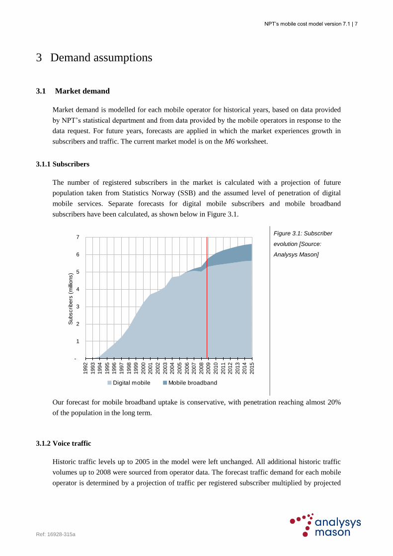
The number of registered subscribers in the market is calculated with a projection of future
population taken from Statistics Norway (SSB) and the assumed level of penetration of digital
mobile services. Separate forecasts for digital mobile subscribers and mobile broadband
subscribers have been calculated, as shown below in Figure 3.1.
-
1
2
3
4
5
6
7
1992
1993
1994
1995
1996
1997
1998
1999
2000
2001
2002
2003
2004
2005
2006
2007
2008
2009
2010
2011
2012
2013
2014
2015
Subscribers
(m
illio
ns)
Digital mobile Mobile broadband
Figure 3.1: Subscriber
evolution [Source:
Analysys Mason]
Our forecast for mobile broadband uptake is conservative, with penetration reaching almost 20%
of the population in the long term.
3.1.2 Voice traffic
Historic traffic levels up to 2005 in the model were left unchanged. All additional historic traffic
volumes up to 2008 were sourced from operator data. The forecast traffic demand for each mobile
operator is determined by a projection of traffic per registered subscriber multiplied by projected
NPT’s mobile cost model version 7.1 | 8
Ref: 16928-315a
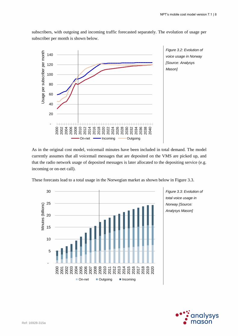
subscribers, with outgoing and incoming traffic forecasted separately. The evolution of usage per
subscriber per month is shown below.
-
20
40
60
80
100
120
1402000
2002
2004
2006
2008
2010
2012
2014
2016
2018
2020
2022
2024
2026
2028
2030
2032
2034
2036
2038
2040
Usage p
er
subscriber
per
month
On-net Incoming Outgoing
Figure 3.2: Evolution of
voice usage in Norway
[Source: Analysys
Mason]
As in the original cost model, voicemail minutes have been included in total demand. The model
currently assumes that all voicemail messages that are deposited on the VMS are picked up, and
that the radio network usage of deposited messages is later allocated to the depositing service (e.g.
incoming or on-net call).
These forecasts lead to a total usage in the Norwegian market as shown below in Figure 3.3.
-
5
10
15
20
25
30
2000
2001
2002
2003
2004
2005
2006
2007
2008
2009
2010
2011
2012
2013
2014
2015
2016
2017
2018
2019
2020
Min
ute
s (
bill
ions)
On-net Outgoing Incoming
Figure 3.3: Evolution of
total voice usage in
Norway [Source:
Analysys Mason]

NPT’s mobile cost model version 7.1 | 9
Ref: 16928-315a
3.1.3 Data traffic
Historic traffic levels up to 2005 already in the model were left unchanged. All additional historic
traffic levels up to 2008 were sourced from operator data, augmented where necessary by NPT‟s
statistics department. Full-year 2009 information has also been incorporated into the v7.1 model.
The forecast of most significance is that for HSPA (mobile broadband) traffic, which is currently
experiencing significant growth in the early phases of take-up. The forecast of total megabytes in
Norway that increases by a factor of six between 2008 and 2012, as shown below in Figure 3.4.
-
2
4
6
8
10
12
14
2006
2007
2008
2009
2010
2011
2012
2013
2014
2015
2016
2017
Tota
l m
egabyte
s (
bill
ions)
-
0.2
0.4
0.6
0.8
1.0
1.2
Month
ly u
sage (
thousands M
B)
Total usage Average usage
Figure 3.4: Evolution of
HSDPA usage in Norway
[Source: Analysys
Mason]
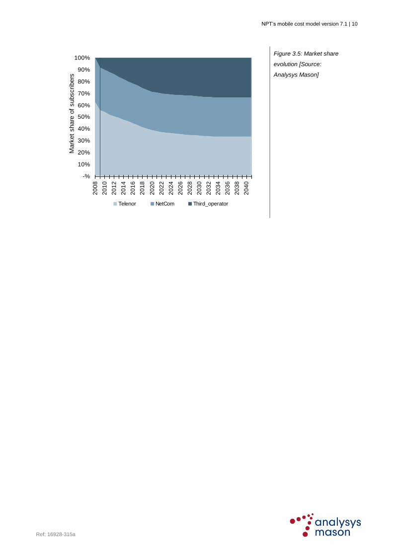
3.2 Market share
The market share of traffic on each infrastructure operator is projected to eventually reach
equalisation at 33%, assuming a third operator entering the market in 2008 and reaching equal
market share in the long term, as shown below in Figure 3.5. This forecast is based on the three-
player market forecast applied in NPT‟s original cost model.
NPT’s mobile cost model version 7.1 | 10
Ref: 16928-315a
-%
10%
20%
30%
40%
50%
60%
70%
80%
90%
100%
20
08
20
10
20
12
20
14
20
16
20
18
20
20
20
22
20
24
20
26
20
28
20
30
20
32
20
34
20
36
20
38
20
40
Mark
et
share
of
subscribers
Telenor NetCom Third_operator
Figure 3.5: Market share
evolution [Source:
Analysys Mason]

NPT’s mobile cost model version 7.1 | 11
Ref: 16928-315a
4 Network assumptions
The main assumptions and choices about radio, core and other aspects of the network design are
described below.
4.1 Radio network
4.1.1 Geotypes
The model considers each Fylke in Norway as a separate geotype. Data on network coverage by
Fylke was supplied to the NPT by each operator through the analysis of each operator‟s network
radio databases.
Each operator has supplied voice traffic data split by geotype, with which the GSM and UMTS
voice and low-speed mobile data networks have been dimensioned; HSDPA mobile broadband
traffic by geotype has been estimated by Analysys Mason on the basis of a population distribution
skewed towards the four major cities in Norway, as shown below in Figure 4.1.
-%
5%
10%
15%
20%
25%
30%
Ake
rsh
us
Au
st-
Ag
de
r
Bu
ske
rud
Fin
nm
ark
He
dm
ark
Ho
rda
lan
d
Mø
re o
g R
om
sd
al
No
rdla
nd
No
rd-T
røn
de
lag
Op
pla
nd
Oslo
Østfo
ld
Ro
ga
lan
d
So
gn
og
Fjo
rda
ne
Sø
r-T
røn
de
lag
Sva
lba
rd
Te
lem
ark
Tro
ms
Ve
st-
Ag
de
r
Ve
stfo
ld
Pro
po
rtio
n b
y F
ylk
e
HSDPA traffic Population
Figure 4.1: Mobile broadband and population distribution [Source: Analysys Mason]
The definition of the geotypes can be found in the A worksheet (for geographical parameters) and
the CovDemIn worksheet (for traffic calculations).

NPT’s mobile cost model version 7.1 | 12
Ref: 16928-315a
4.1.2 Coverage
Coverage was determined on the basis of the radio database of each of the operator‟s networks, as
submitted to the NPT as part of the data request. From this database, the area covered at a signal
strength of –94dBm was calculated: this strength represents approximate outdoor coverage.
Coverage calculations were made for the following sets of frequencies:
GSM900
GSM1800
GSM900+GSM1800 (i.e. GSM)
UMTS.
Indoor coverage, in terms of area and population, reflected by a higher signal strength, is
commensurately lower, though not used to drive network deployment in the model except for the
initial coverage of the third entrant operator reflected in the v7.1 model.
In the initial network roll-out years, additional sites are assumed to be rolled out to maximise the
area covered, with little or no overlap between cells. In the later years, sites are deployed for infill
purposes. These sites fill in the gaps in wide-area coverage and improving the contiguousness of
the network. They consequently have a lower cell radius, reflecting the smaller uncovered areas
which these cells satisfy. This concept is shown in Figure 4.2 for the operators‟ GSM networks:

NPT’s mobile cost model version 7.1 | 13
Ref: 16928-315a
Coverage site
Infill site
Time
Are
a c
ove
red
(k
m2)
rcoverage
rinfill
Approx
year
1997
80
:20
are
a r
ule
Figure 4.2: Wide-area
GSM coverage and infill
[Source: Analysys
Mason]
The coverage profile of the GSM network is defined for each operator, on the basis of 900MHz
frequencies, using the inputs from the original (v4) model. These inputs have been updated for the
period 2005–2008 using outputs of the GSM coverage recalculation performed by NPT in 2009.
For the modelled UMTS networks, the approach to wide-area and infill coverage has been
modified slightly. The UMTS model assumes the following roll-out process:
“wide-area” coverage of the urban areas in each Fylke is deployed using 2100MHz spectrum
“infill” coverage of the urban areas in each Fylke is deployed using 2100MHz spectrum
rural coverage in each Fylke is deployed using UMTS900 equipment, on the assumption that
as GSM frequencies become unloaded, they can be re-farmed for a 900MHz UMTS
deployment.
Therefore, the first two parts of this coverage roll-out are similar to the GSM network algorithm,
albeit with alternative parameters reflecting the proportion of population (and hence area) and cell

NPT’s mobile cost model version 7.1 | 14
Ref: 16928-315a
radius used for the deployment. The third part of UMTS coverage aims to replicate GSM coverage
in order that the GSM network may be shut-down.
This concept is shown in Figure 4.3 below for the operators‟ UMTS networks. Although the roll-
out using 2100MHz spectrum only covers approximately 25% of the Norwegian land area, it
reaches more than 90% of the population. UMTS900 is then used to increase the UMTS coverage
to equal to GSM coverage, but only covers the remaining 5–10% of population across a large area
of the country.
Time
Are
a c
overe
d (
km
2)
e.g. 25% area of all Fylke
e.g +60% area of Fylkee.g. +2% area of all Fylke
Time
Po
pu
lati
on
co
vere
d (
km
2)
e.g. 90-95% population of all Fylke
~+1% population of all Fylke
e.g. +5% population of all FylkeKey
2100MHz urban wide area
2100MHz urban infill
900MHz rural
Figure 4.3: UMTS coverage and infill [Source: Analysys Mason]
The parameters determining these calculations can be found in the NtwDesBase and NtwDesSlct
worksheets.
4.1.3 Mobile broadband
In order to offer mobile broadband services using UMTS, the model includes three levels of high-
speed packet data service:
HSDPA 3.6Mbit/s: deployed in the first carrier at all UMTS sites using 32 channels per
NodeB with 16QAM coding
HSDPA 7.2Mbit/s with HSUPA 1.5Mbit/s: in addition to the first level of service, a
proportion of NodeBs are upgraded with an additional 64 channels per NodeB in the second
5MHz carrier to support HSDPA along with 32 channels per NodeB for HSUPA (2 codes
Spreading Factor 4)
HSDPA 14.4Mbit/s with HSUPA 1.5Mbit/s: the model can assume that those NodeBs
deployed with HSDPA7.2 are then upgraded after an assumed number of years to use an
additional 64 channels per NodeB in the second 5MHz carrier to support HSDPA at
14.4Mbit/s.

NPT’s mobile cost model version 7.1 | 15
Ref: 16928-315a
4.1.4 Repeater sites
Repeater sites are deployed to serve special areas that cannot be covered by other types of sites.
The model considers two types of repeater sites: wide-area repeaters and tunnel repeaters.
Based on a comparative analysis of the deployment actually undertaken by operators in Norway,
the number of wide-area repeaters is based on a percentage of sites required for coverage purposes.
It is assumed that wide-area repeaters are radio repeaters – i.e. they have a receive and a re-
transmit antenna. Repeaters for coverage are deployed separately in the 2G and 3G networks.
Coverage of road and rail tunnels is an important part of Norwegian mobile networks. Given the
fact that the number of tunnels in Norway is finite, the number of 2G and 3G tunnel repeaters are
both entered into the model as an explicit inputs.
These roll-outs are defined in the NtwDesBase worksheet.
4.1.5 Sectorisation and overlay of sites
Radio sites deployed in Norway are mainly for coverage purposes, and traffic levels for the
average site are generally low by European standards. As a result, such GSM sites are frequently
omni-sectored, with subsequent sectorisation and overlay of DCS1800 spectrum occurring
predominantly for capacity purposes only in towns and cities.
Capacity dimensioning is carried out with reference to parameters including:
radio blocking probability (1% to 5% depending on cell layer)
approximately 8% of daily voice traffic is in the busy hour (typically 16:00-17:00 on a
weekday) and approximately 80% of annual traffic occurs during weekdays
typical maximum equipment utilisation parameters.
The GSM network is dimensioned using the traffic channel (TCH) Erlang load from voice and
GPRS traffic. The process for calculating the GSM capacity, sectorisation and overlay of sites with
secondary spectrum is shown below in Figure 4.4.

NPT’s mobile cost model version 7.1 | 16
Ref: 16928-315a
Omni site for coverage,
1 TRX
Sectorisation of Omni
sites
Overlay of sectorised
sites with DCS (if
available)
TRX upgrade to
maximum allowed
Deployment of further
sites (with DCS if
available)
TRX TRXTRXTRXTRX
TRXTRXTRXTRX
TRXTRXTRXTRX
TRXTRXTRXTRX
TRXTRXTRXTRX
TRXTRXTRX
TRXTRXTRX
TRXTRXTRXTRX
TRXTRXTRXTRX
TRXTRXTRX
TRXTRXTRX
+ tunnel sites
+ coverage
repeaters
Figure 4.4: GSM radio
network deployment
[Source: Analysys
Mason]
The UMTS network is dimensioned with the Release-99 channel element load produced by voice
and low-speed data Erlangs. The UMTS network is expanded with increasing traffic in terms of
channel kit (CK) and additional carriers per site. It is assumed that in order to accommodate cell
breathing effects, the UMTS coverage networks deployed by the operators are sufficient to carry
forecast voice and data traffic loads.
In the case of the UMTS network, 2100MHz sites are deployed predominantly in urban areas and
are therefore deployed “fully-sectorised” according to the average sectorisation of 2100MHz sites
(between 2 and 3 depending on operator data). In the later years within the model, UMTS900 sites
are deployed as omni-sectored sites in rural parts of each Fylke.
The number of sites deployed have been calibrated against operators‟ actual numbers separately
for both the GSM and UMTS networks.
Capacity and sectorisation inputs can be found in the NtwDesBase worksheet.
4.1.6 Site types
Operators utilise a mix of shared, third-party and owned sites. The model considers the proportion
of three types of site deployment – in order to capture the different costs associated with site
acquisition, civil and ancillary equipment. The three types are shown in Figure 4.5.

NPT’s mobile cost model version 7.1 | 17
Ref: 16928-315a
Own tower site Third-party tower site Third-party roof-top site
(blue shading denotes own equipment; grey shading denotes third-party assets)
Own tower site Third-party tower site Third-party roof-top site
(blue shading denotes own equipment; grey shading denotes third-party assets)
Figure 4.5: Site types
[Source: Analysys
Mason]
Existing GSM sites may be suitable for adding UMTS NodeB equipment. We specify the
proportion of 2G sites suitable for this upgrade (currently estimated to be 85%–100%). For each
year in the model, the total number is calculated for:
sites with only 2G technology deployed (2G-only)
sites with only 3G technology deployed (3G-only)
sites with both 2G and 3G technologies deployed (2G/3G).
Site type proportions can be found in the NtwDesBase worksheet.
4.1.7 Backhaul configuration
The GSM backhaul configuration is modelled on the basis of the percentage of sites in each Fylke
which require microwave (typically 8Mbit/s units, though there may also be some E1 connections)
or leased-line (either 64kbit/s or 2Mbit/s E1 links) backhaul. This is shown in Figure 4.6.
BSC
8Mbit/s
microwave
(n E1 part
filled)
n E1 leased lines
per site on average
64kbit/s leased line
for remote site
(upgradeable to E1)
DXX
DXX
cluster Tunnel sites
n E1 leased lines
per site on average
~1.5 TRX
E1
DXX
~1.5 TRX
E1
E1
Figure 4.6: GSM
backhaul configuration
[Source: Analysys
Mason]
DXX access nodes are deployed according to 64kbit/s links, and are modelled to persist in the
network even when the 64kbit/s links are replaced with a higher capacity E1. DXX cluster nodes

NPT’s mobile cost model version 7.1 | 18
Ref: 16928-315a
are deployed on the basis of a number of access nodes per cluster node. This ratio is based on data
submitted by each operator.2
The UMTS backhaul configuration is similar, with the exception that 64kbit/s links are not used at
all. All NodeB‟s require at least one E1 for R99 traffic; in addition, the NodeB HSDPA throughput
(plus an estimated IP overhead) must be provisioned in the backhaul capacity of each site. This is
shown below in Figure 4.7.
8Mbit/s
microwave
(n E1 part
filled)
Tunnel sites
n E1 leased lines per site on average, higher
in areas with HSDPA7.2 deployment
Sectors/CE
E1
E1
E1
Sectors/CE
E1
RNC
Figure 4.7: UMTS
backhaul configuration
[Source: Analysys Mason
]
These assumptions can be found in the NtwDesBase worksheet.
4.1.8 BSC deployment
The number of BSC locations per Fylke is defined over time. For historical years it is based on
data supplied by the operators, and for forecast years it is assumed to remain constant according to
the last year of historical data.
The number of BSCs are driven by the number of transceivers (TRX) in the network. The TRX
calculated in each Fylke are logically mapped onto a particular Fylke‟s BSC location according to
network information supplied by the operators. This is shown on a theoretical basis in Figure 4.8
below.
2 We have not modelled DXX units for NetCom because they do not appear to conform to this deployment logic. Instead, the costs of
NetCom’s DXX units are included in the cost of other radio and transmission equipments.

NPT’s mobile cost model version 7.1 | 19
Ref: 16928-315a
BSC
BSC
TRXTRXTRXTRX
TRXTRXTRXTRX
TRXTRXTRXTRX
TRXTRXTRXTRX
TRXTRXTRXTRX
TRXTRXTRXTRX
TRXTRXTRXTRX
TRXTRXTRXTRX
TRXTRXTRXTRX
TRXTRXTRXTRX
TRXTRXTRXTRX
Fylke 1Fylke 2
Fylke 3
Figure 4.8: BSC
deployment [Source:
Analysys Mason]
BSC capacity is defined in terms of number of TRXs, as supplied by each operator. The inputs
associated with this deployment can be found in the NtwDesBase worksheet.
4.1.9 Remote BSCs and associated BSC–MSC links
Remote BSC locations are modelled to occur when the number of BSC locations in a Fylke is
greater than the number of MSC locations in that Fylke (each MSC location logically has a co-
located BSC location).
In a Fylke in which there are no MSC locations, all BSCs in the Fylker are remote. When there are
MSC locations in the Fylke, is assumed that there is one remote BSC per remote BSC location,
and all remaining BSC required are co-located with the MSC(s).
Remote BSCs are attached to the nearest MSC – which will either be in the same Fylke, or the
nearest Fylke by distance.
The traffic transiting through these BSCs is backhauled to the MSC using E1 leased lines. The
length of these E1 links is determined by the Fylke-Fylke distance matrix, or the estimated
internal-Fylke distance. This is shown below in Figure 4.9.

NPT’s mobile cost model version 7.1 | 20
Ref: 16928-315a
BSCBSC
MSC
i km
n E1
leased lines16kbit/s
16kbit/s
nearest d km
BSC
Figure 4.9: BSC–MSC
transmission for remote
BSCs [Source: Analysys
Mason]
4.1.10 RNC deployment
The number and location of RNC switches is specified by Fylke, according to each operator‟s
network topology. Typically, RNCs are only deployed in the major cities of Norway (and possibly
in multiple locations in Oslo).
The number of RNCs beyond this initial deployment in the major cities is determined by the
maximum of three measures:
Mbit/s traffic in the voice busy hour (where voice traffic is expressed according to 12.2kbit/s
per Erlang, and added to both low-speed and high-speed Mbit/s)
incoming E1 ports
number of NodeBs.
Each of these measures is logically mapped onto a particular Fylke‟s RNC location, in the same
way as for BSCs (see section 4.1.8). The inputs associated with RNC deployment can be found in
the NtwDesBase worksheet.
4.1.11 RNC links to the core network
RNC switches are considered „remote‟ when they are deployed in a Fylke without a corresponding
voice MSC or MSS switch. Unless specified by the RNC location and MSC/MSS location input
matrices, it is assumed that RNC switches are always deployed together in a Fylke – i.e. in one
building, and not dispersed throughout the Fylke.
Remote RNCs require connectivity to the core network, with either:
links to legacy MSC sites for the voice plus data Mbit/s load presented at the remote RNCs
links to the layered core network, with circuit-switched links to MSS sites for voice load, and
packet-switched links to the packet routeing layer for mobile data traffic.

NPT’s mobile cost model version 7.1 | 21
Ref: 16928-315a
These two types of connectivity are dimensioned in the following ways.
Legacy network The voice and data Mbit/s passing through each remote RNC is mapped to
the nearest MSC switching location (determined by a distance-aware matrix
calculation) and dimensioned with either E1 or STM–1 links (subject to a
maximum utilisation percentage). Redundant links are deployed for
resilience purposes.
Layered network The voice BHE passing through each remote RNC is mapped to the nearest
MGW location (determined by a distance-aware matrix calculation) and
dimensioned using STM–1 links (subject to a maximum utilisation
percentage). Redundant links are deployed for resilience purposes.
The data Mbit/s passing through each remote RNC is mapped to the nearest
packet routeing location (determined by a distance-aware matrix
calculation) and dimensioned using STM–1 links, subject to a maximum
utilisation percentage.
This layered architecture is illustrated below in sections 4.2.3–4.2.4.
4.2 Core network
For each 2G/3G operator, it is assumed that their networks are deployed in the following order:
2G network (radio and core)
3G radio network (with software upgrade to 2G MSC layer to handle 3G traffic)
layered core network, with the shut-down of the legacy 2G core network
shut-down of the 2G radio network.
The model accommodates both types of core network – i.e. the legacy core of meshed MSCs (and
meshed TSCs if deployed), as well as a layered core with a separate circuit-switched layer (MGWs
on a transmission mesh or ring) for voice and packet-switched layer for data (using meshed packet
routers and GSNs).
4.2.1 Legacy MSC/VLR deployment
MSC deployment responds to three demand drivers: ports, processing and locations. Processor
load is assessed based on the number of calls, SMS and location updates of each type that need to
be switched. This determines the number of CPUs required. When the 3G network is deployed, but
before the switch to a layered circuit/packet architecture, MSCs must be upgraded to support both
2G and 3G voice and SMS switching. This is modelled as a software upgrade to each MSC.
NPT’s mobile cost model version 7.1 | 22
Ref: 16928-315a
Transmission requirements determine the number of E1 port cards required to support
transmission to and from the MSCs. Each MSC has a limited capacity in terms of ports.
Finally, the model ensures that the number of MSCs is at least equal to the number of specified
MSC locations.
4.2.2 Legacy transit layer
A transit layer may be deployed for high volumes of traffic, and is controlled by the input of transit
switching centre (TSC) locations over time. When more than one Fylke contains a TSC, the model
switches to a transit layer hierarchy. The transit layer consists of dedicated switches that are above
standard MSCs in the logical hierarchy of the network. All the traffic between MSCs is handled by
the transit layer first. With a transit layer, all MSCs outside the transit layer are linked to two TSCs
for redundancy.
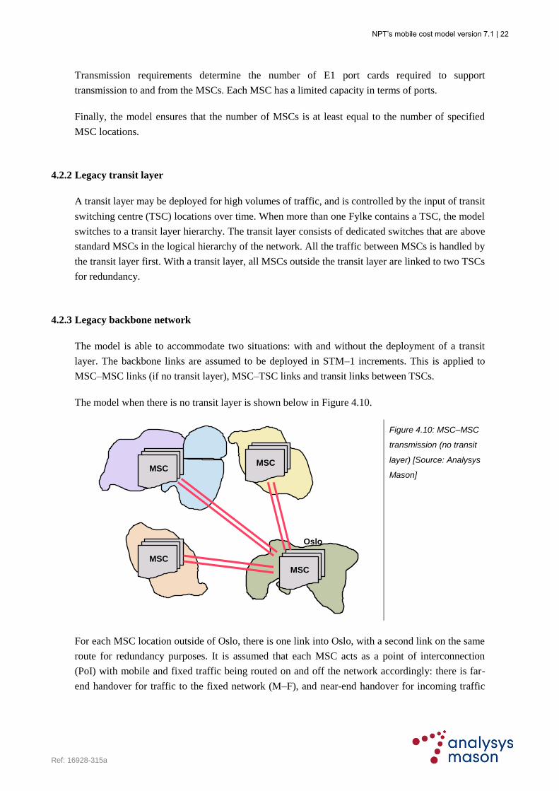
4.2.3 Legacy backbone network
The model is able to accommodate two situations: with and without the deployment of a transit
layer. The backbone links are assumed to be deployed in STM–1 increments. This is applied to
MSC–MSC links (if no transit layer), MSC–TSC links and transit links between TSCs.
The model when there is no transit layer is shown below in Figure 4.10.
MSCMSC
MSC
MSC
Oslo
Figure 4.10: MSC–MSC
transmission (no transit
layer) [Source: Analysys
Mason]
For each MSC location outside of Oslo, there is one link into Oslo, with a second link on the same
route for redundancy purposes. It is assumed that each MSC acts as a point of interconnection
(PoI) with mobile and fixed traffic being routed on and off the network accordingly: there is far-
end handover for traffic to the fixed network (M–F), and near-end handover for incoming traffic

NPT’s mobile cost model version 7.1 | 23
Ref: 16928-315a
into the network (F–M and M–M). When there is more than one MSC deployed within Oslo, a
ring structure is also deployed to connect them.
MSC
MSC
MSC
n STM1
n STM1
MSC
MSC
MSC
n STM1
n STM1
Figure 4.11: Deployment
of the Oslo ring when
there is no transit layer
[Source: Analysys
Mason]
For the intra-Oslo MSC–MSC transmission, 3km leased lines per MSC of n STM–1 per link are
modelled. Their capacity is driven by the amount of traffic that is carried over MSCs in Oslo.
The model calculates the effect of the deployment of a transit layer in a logically similar fashion,
displayed in Figure 4.12.
MSCMSC
MSCTransit
Fylke
nearest TSC
Figure 4.12: MSC–TSC
transmission with the
deployment of a transit
layer [Source: Analysys
Mason]
The nearest TSC is identified for each Fylke with MSCs but no TSCs. There is one MSC–TSC
link per MSC location, with a second link per route dimensioned for redundancy purposes.
It is assumed similarly that each MSC and TSC acts as a point of interconnection (PoI) with
mobile and fixed traffic being routed on and off the network accordingly. There is far-end
handover for traffic to the fixed network (M–F), and near-end handover for incoming traffic into
the network (F–M and M–M).
A fully meshed TSC layer is modelled with n STM–1 units per route. However, the physical
structure of the transit layer modelled is that of a national ring and the Oslo ring.

NPT’s mobile cost model version 7.1 | 24
Ref: 16928-315a
TSC
TSC
TSC
TSC
Oslo
TSC
TSC
Figure 4.13: Fully
meshed transit layer
[Source: Analysys
Mason]
The length of the rings is calculated from TSC locations, including Oslo.
4.2.4 Layered circuit-switched network
MSS switches are deployed at each MSS site, according to processor load (calls, SMS and location
updates) and utilisation. MGW switches are deployed in redundant pairs at each MSS.
Inter-switch and VMS voice Erlangs are used to determine MGW–MGW STM–1 ports between:
MGW sites within Oslo (if there are multiple MSS locations in Oslo)
co-sited MGW outside of Oslo
MGW sites outside of Oslo.
This is illustrated below in Figure 4.14. Physical STM–1 links are only dimensioned between sites.

NPT’s mobile cost model version 7.1 | 25
Ref: 16928-315a
Oslo
MGW
MGW
MGW
MGW
MGW
MGWMGW
MGW
Intra-site MGW
links outside Oslo
Inter-site MGW links
outside Oslo on a
redundant ring
Inter-MGW
links in Oslo
on a ring
Figure 4.14: Modelled
MGW–MGW links and
ports [Source: Analysys
Mason]
4.2.5 Layered packet-switched network
A packet data router is deployed at each packet-switching location (these may be SGSN switches
or IP routers, depending on the choice of network configuration). The proportion of busy hour
Mbit/s from mobile data traffic which crosses the packet data network is then used to dimension a
fully meshed packet routeing network. STM–1 links connect the RNCs to these packet data
routers, as shown below in Figure 4.15.

NPT’s mobile cost model version 7.1 | 26
Ref: 16928-315a
Oslo
Router
RNC
Router
Router
Router
RNC
RNC RNCRNC
RNC
RNC
Figure 4.15: Modelled
layered packet-switch
architecture [Source:
Analysys Mason]
4.3 Other network elements
We have included explicit calculations of what we believe are the remaining significant network
element deployments: HLR, AUC, EIR, network management systems, licence fees, intelligent
network (IN) system, billing system, VMS, packet data and SMS infrastructure.
4.4 Non-network elements
The original (v4) model included explicit bottom-up modelling of retail costs such as marketing
and customer care. Ultimately, these costs were used to share business overheads between network
and retail functions according to a cost-based equi-proportional mark-up (EPMU). The
handset/acquisition component of retail costs was excluded from the business overhead mark-up.
Retail aspects have now been removed in the v6 model. Business overhead expenditure remain in
the model, but are now marked-up directly onto network activities using a ratio of 75:25 (derived
from the v4 model). This modification has been made to reduce the complexity of the model
without materially affecting the wholesale cost results. Business overhead expenditures are now
modelled as:
a fixed annual capital and operating expenditure
a subscriber-dependent operating expenditure.
NPT’s mobile cost model version 7.1 | 27
Ref: 16928-315a
4.5 Third operator
In the market forecast for the original (v4) model, we assumed that a third infrastructure operator
would enter the market and gain market share parity with the established operators in the long
term. In the upgraded (v6 and v7.1) model, we have explicitly dimensioned the network of this
new entrant. This network can be selected by choosing “Third operator” on the Ctrl worksheet.
Several key assumptions have been made regarding the third operator deployment:
it is a combined 2G/3G operator:
– GSM is launched in 2008 to cover approximately 98% population of six Fylker with major
cities in Norway3, completed in one year, with 20% of this coverage area completed with
in-fill sites
– GSM is shut down in 2020
– UMTS is deployed at least 99.99% of population in all Fylker (except Svalbard), using
sectorised 2100MHz urban networks and omni-sectored 900MHz rural NodeBs (using the
same coverage calculation methodology as for the other operators)
– UMTS coverage to the initial population covered provides indoor-quality coverage
– all 2G sites are reused for NodeB deployments
– HSDPA 3.6 is deployed on all NodeBs
– A proportion of 2100MHz NodeBs are upgraded to HSDPA 7.2 from 2009 onwards, with
99% of those in Oslo upgraded, 66% of those in Hordaland, Rogaland and Sør-Trøndelag
upgraded and 33% of those in Akershus and Vestfold upgraded
– All HSDPA 7.2 sites are upgraded further to HSDPA 14.4 from 2011
– the backhaul network uses a combination of microwave links and leased lines
– BSCs and RNCs are located in each of the six main Fylker
8% of daily voice traffic occurs in the voice busy-hour
9% of daily HSDPA traffic occurs in the data busy-hour
voice and non-HSDPA traffic by Fylke is distributed according to covered population
HSDPA traffic by Fylke is distributed as per section 4.1.1
a layered architecture is deployed for the core network from launch, with all major switching
sites in Oslo.
The third operator is set up using assumptions that are distanced from operator data, allowing this
model to be distributed to all industry parties.
4.6 MVNO networks
The mobile virtual network operators (MVNOs) in Norway perform a number of network
functions themselves, whilst renting radio access capacity on one of the networks. The exact way
in which each MVNO provides this functionality varies – some have dedicated Norwegian
3 We assume Akershus, Hordaland, Oslo, Rogaland, Sør-Trøndelag and Vestfold

NPT’s mobile cost model version 7.1 | 28
Ref: 16928-315a
facilities, while others lease their activities from other operators outside of Norway. We have
modelled the Norwegian MVNOs in the model on the basis of being standalone Norwegian
infrastructure-based operators.
The list of operators that can be selected in the model include four MVNOs: Tele2, Network
Norway, TDC and Ventelo. It should be noted that when one of these operators is selected, various
stages of the network design calculation will not calculate, particularly in the radio layer – this
only occurs for elements that are not required by MVNOs, which are then excluded on the FullNw
worksheet prior to the cost calculation.
MVNOs are modelled with the network elements listed in Figure 4.16 below.
MSC (and associated ports / software) Intelligent network (IN) Figure 4.16: MVNO
assets dimensioned in
the model [Source:
Analysys Mason ]
HLR and upgrades Billing system
GGSN AUC
SGSN EIR
SMSC
MMSC

NPT’s mobile cost model version 7.1 | 29
Ref: 16928-315a
5 Expenditure calculations
5.1 Purchasing, replacement and capex planning period
The network design algorithms compute the network elements that are required to support a given
demand in each year.
In order for these elements to be operational when needed, they need to be purchased in advance,
in order to allow provisioning, installation, configuration and testing before they are activated.
This is modelled for each asset by inputting a planning period between 0 (no planning required)
and 24 months. In the early years of network deployment (1992–1996) the purchasing of assets for
Telenor and NetCom has been redistributed to reflect a „Phase 1 deployment‟ as might be
contracted to an equipment vendor.
In order to calculate the number of assets to be purchased in each year, the model computes the
number of additional assets that need to be installed to provide incremental capacity, and includes
the amount of equipment that has reached the end of its lifetime and needs to be replaced.
5.2 Network closure
The model now includes the functionality to reduce and shut down the GSM network as its
volumes migrate to UMTS. This shut-down is determined by the voice migration profile on the M6
worksheet. Currently, this migration is predicted to be complete by 2020 for all infrastructure
operators.
The GSM radio and core layers can be shut down separately: this allows the legacy core network
to be migrated to a next-generation architecture prior to the de-activation of the GSM radio
network. The shut-down of the core network (and launch of a next-generation architecture) can be
changed using the inputs at the top of the NtwDesBase worksheet.
During the period that traffic is being reduced on a group of network elements (e.g. reducing GSM
load as migration occurs), the model contains the functionality for “stranded” equipment to be
either:
kept in the network until the last year of operation and then removed
removed from the network as traffic load reduces (either in the same year, or 1 year later, or 2
years later).
This functionality is captured by the retirement delay input (sheet L) of 0, 1, 2 or “100” years until
removal.

NPT’s mobile cost model version 7.1 | 30
Ref: 16928-315a
The recovery of expenditures on GSM and legacy core equipment is confined to the period of their
operation – i.e. UMTS services do not contribute to GSM cost recovery, and traffic after the legacy
core shut-down does not recover any of the legacy core expenditures (instead it recovers layered
core expenditures).
5.3 MEA equipment unit price
The price paid for network assets varies over time. In the economic costing approach, the modern
equivalent asset provides the appropriate cost basis for purchasing. Real-term price trends are
applied to 1992 prices to reflect the evolution of the modern technology prices over past and future
time. MEA price evolution also provides an important input into the economic depreciation, as
explained in section 6. Price trends are populated with Analysys Mason estimates rather than
operator data.
The model can now calculate in the real terms currency of any year: this can be changed on the
Ctrl worksheet. However, unit cost inputs are specified in real 2005 NOK (as per the v4 model).
5.4 Phase 1 distribution of expenditures for Telenor and NetCom
Operators‟ GSM expenditures only begin in 1993/1994. However, Telenor and NetCom began to
install their GSM network structures in 1992. The model also includes a plan-ahead period for
each asset, resulting in assets being purchased up to 18–24 months in advance of this date.
Consequently, a Phase 1 expenditure ramp is applied, which re-distributes the purchases that are
incurred over the period 1990–1996. The Phase 1 ramp distributes the purchases so that the
modelled expenditure profile is in line with that actually incurred by each operator.
NPT’s mobile cost model version 7.1 | 31
Ref: 16928-315a
6 Annualisation of expenditure
This section describes the implementation of the economic depreciation algorithm used in NPT‟s
mobile cost model. It details both the economic rationale for using this algorithm and the
calculations themselves.
6.1 Rationale for using economic depreciation
Economic depreciation is a method for determining a cost recovery that is classed as being
economically rational, in that it:
reflects the underlying costs of production
reflects the output of network elements over their lifetime.
The first factor relates the cost recovery to that of a new entrant to the market, which would be
able to offer the services based on the current costs of production.
The second factor relates the cost recovery to the „lifetime‟ of a mobile business – in that
investments and other expenditures are in reality made throughout the life of the business
(especially large, upfront investments) on the basis of being able to recover them from all demand
occurring in the lifetime of the business. New entrants to the market would also be required to
make these large upfront investments, and recover costs over the lifetime in a similar fashion to the
existing operators. (This is based on the realistic assumption that new entrants to the market face
the same systemic barriers to entry as faced by the existing operators, and would not realistically
be able to instantaneously capture the entire market of an operator, i.e. the market is less than fully
contestable).
These two factors are not reflected in accounting-based depreciation, which simply considers when
an asset was bought, and over what period the investment costs of the asset should be depreciated.
Fundamentally, the implementation of economic depreciation utilised in the model is based on the
principle that all (efficiently) incurred costs should be fully recovered, in an economically rational
way.
Full recovery of all (efficiently) incurred costs is ensured by checking that the present value (PV)
of actual expenditures incurred = the PV of economic costs recovered.
An allowance for capital return earned over the lifetime of the business, specified by the WACC,
is also included in the resulting costs.
NPT’s mobile cost model version 7.1 | 32
Ref: 16928-315a
6.2 Implementation of economic depreciation principles
The economic depreciation algorithm recovers all efficiently incurred costs in an economically
rational way by ensuring that the total of the revenues generated across the lifetime of the business
are equal to the efficiently incurred costs, including cost of capital, in PV terms.
More specifically, for every asset class, in every year, the algorithm recovers the proportion of
total cost (incurred across the lifetime of the business) that is equal to the revenue generated in that
year as a proportion of the total revenue generated (across the lifetime of the business) in PV
terms.
PV calculation
The calculation of the cost recovered through revenues generated needs to reflect the value
associated with the opportunity cost of deferring expenditure or revenue to a later period. This is
accounted for by the application of a discount factor on future cash flow, which is equal to the
weighted average cost of capital (WACC) of the modelled operator.
The business is assumed to be operating in perpetuity, and investment decisions are made on this
basis. This means that it is not necessary to recover investments within a particular time horizon,
for example the lifetime of a particular asset, but rather throughout the lifetime of the business. In
the model, this situation is approximated by explicitly modelling a period of 50 years. At the
discount rate applied, the PV of investments in the last year of the model is fractional and thus any
perpetuity value beyond 50 years is regarded as immaterial to the final result.
Cost recovery profile
The costs incurred over the lifetime of the network are recovered in line with the revenues
generated by the business. The revenues generated by an asset class are a product of the demand
(or output) supported by that asset class and the price per unit demand.
In the modelled environment of a competitive market, the price that will be charged per unit
demand is a function of the lowest cost of supporting that unit of demand, thus the price will
change in accordance with the costs of the factors of production. Put another way, if a low-cost
asset could support a particular service, then the price charged for the same service supported by a
more expensive asset would be reflective of the costs of the lower-cost asset or else a competitor
would supply the service using the lower-cost asset to capture the associated supernormal profits.
The shape of the revenue line (or cost recovery profile) for each asset class is thus a product of the
demand supported (or output) of the asset and the profile of replacement cost (or modern
equivalent asset price trend) for that asset class.
NPT’s mobile cost model version 7.1 | 33
Ref: 16928-315a
Capital and operating expenditure
The efficient expenditure of the operator comprises of all the operator‟s efficient cash outflows
over the lifetime of the business, meaning that capital and operating expenditures are not
differentiated for the purposes of cost recovery. As stated previously, the model considers costs
incurred across the lifetime of the business to be recovered by revenues across the lifetime of the
business. Applying this principle to the treatment of capital and operating expenditure leads to the
conclusion that they should both be treated in the same way since they both contribute to
supporting the revenues generated across the lifetime of the operator.
Cost recovery by deployment
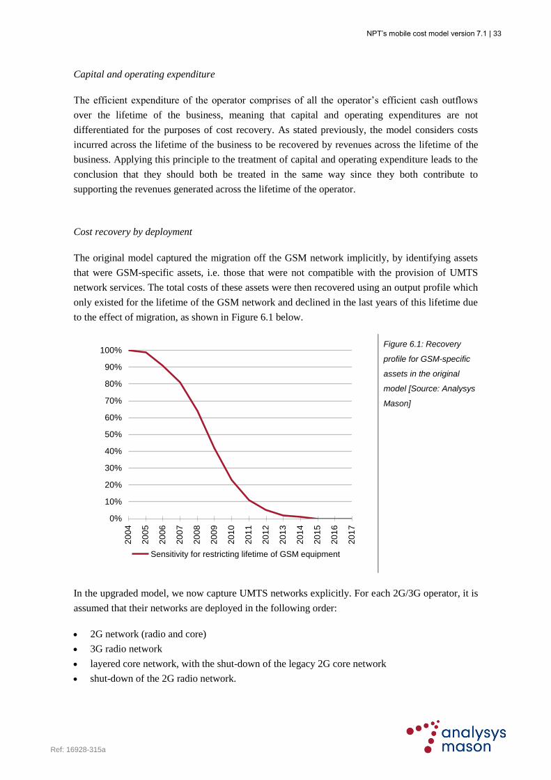
The original model captured the migration off the GSM network implicitly, by identifying assets
that were GSM-specific assets, i.e. those that were not compatible with the provision of UMTS
network services. The total costs of these assets were then recovered using an output profile which
only existed for the lifetime of the GSM network and declined in the last years of this lifetime due
to the effect of migration, as shown in Figure 6.1 below.
0%
10%
20%
30%
40%
50%
60%
70%
80%
90%
100%
20
04
20
05
20
06
20
07
20
08
20
09
20
10
20
11
20
12
20
13
20
14
20
15
20
16
20
17
Sensitivity for restricting lifetime of GSM equipment
Figure 6.1: Recovery
profile for GSM-specific
assets in the original
model [Source: Analysys
Mason]
In the upgraded model, we now capture UMTS networks explicitly. For each 2G/3G operator, it is
assumed that their networks are deployed in the following order:
2G network (radio and core)
3G radio network
layered core network, with the shut-down of the legacy 2G core network
shut-down of the 2G radio network.
NPT’s mobile cost model version 7.1 | 34
Ref: 16928-315a
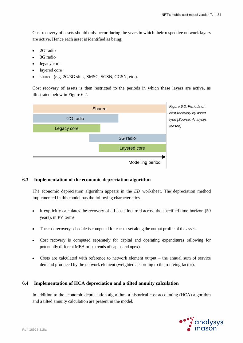
Cost recovery of assets should only occur during the years in which their respective network layers
are active. Hence each asset is identified as being:
2G radio
3G radio
legacy core
layered core
shared (e.g. 2G/3G sites, SMSC, SGSN, GGSN, etc.).
Cost recovery of assets is then restricted to the periods in which these layers are active, as
illustrated below in Figure 6.2.
Shared
2G radio
3G radio
Legacy core
Layered core
Modelling period
Figure 6.2: Periods of
cost recovery by asset
type [Source: Analysys
Mason]
6.3 Implementation of the economic depreciation algorithm
The economic depreciation algorithm appears in the ED worksheet. The depreciation method
implemented in this model has the following characteristics.
It explicitly calculates the recovery of all costs incurred across the specified time horizon (50
years), in PV terms.
The cost recovery schedule is computed for each asset along the output profile of the asset.
Cost recovery is computed separately for capital and operating expenditures (allowing for
potentially different MEA price trends of capex and opex).
Costs are calculated with reference to network element output – the annual sum of service
demand produced by the network element (weighted according to the routeing factor).
6.4 Implementation of HCA depreciation and a tilted annuity calculation
In addition to the economic depreciation algorithm, a historical cost accounting (HCA) algorithm
and a tilted annuity calculation are present in the model.

NPT’s mobile cost model version 7.1 | 35
Ref: 16928-315a
The calculation flow for the HCA depreciation algorithm is set out below in Figure 6.3.
Net Book
Value
Asset
lifetimes
Real opex
Real
investment
Inflation
Nominal
investment
Gross Book
Value
Annual
depreciation
Nominal opex
Inflation
Nominal
discount rate
Annual cost of
capital
Total annual
cost - nominal
(HCA)
Total annual
cost - real
(HCA)
Inflation
Economic
depreciation
Network
element unit
costs (HCA)
Network
element unit
costs (ED)
Com
pare
Figure 6.3: HCA algorithm [Source: Analysys Mason]
The HCA algorithm calculates the total nominal annual cost in each year using the annual
depreciation from the gross book value of nominal investments; the annual cost of capital; and the
nominal operating expenditure. These costs are converted back into real terms, and can be
compared with the cost result of the economic depreciation algorithm.
The calculation flow for the tilted annuity depreciation algorithm is set out below in Figure 6.4.

NPT’s mobile cost model version 7.1 | 36
Ref: 16928-315a
Gross
replacement cost
of network (capex)Network
equipment
deployment
Unit investment
costs
Capex MEA price
trend
Asset series
(lifetime)
Economic
depreciation
Forward looking
real discount rate
divider
Network element
output
Annualised capex
and opex cost per
unit output
MTR (2005)
Tilted annuity
profile
Total recovery
from asset
Annualised cost
per year
Opex in 2005Annualised capex
2005
Routeing factors
for incoming callsMTR (2005)
Com
pare
Gross
replacement cost
of network (capex)Network
equipment
deployment
Unit investment
costs
Capex MEA price
trend
Asset series
(lifetime)
Economic
depreciation
Forward looking
real discount rate
divider
Network element
output
Annualised capex
and opex cost per
unit output
Network element
output
Annualised capex
and opex cost per
unit output
MTR (2005)
Tilted annuity
profile
Total recovery
from asset
Annualised cost
per year
Tilted annuity
profile
Total recovery
from asset
Annualised cost
per year
Opex in 2005Annualised capex
2005Opex in 2005
Annualised capex
2005
Routeing factors
for incoming callsMTR (2005)
Routeing factors
for incoming callsMTR (2005)
Com
pare
Figure 6.4: Tilted annuity calculation [Source: Analysys Mason]
The tilted annuity calculation determines the gross cost of replacing the entire network at 2005
prices. The capital cost recovery profile is tilted according to the forecast capex MEA price trend,
resulting in an annualised cost for the year 2008. Taking the incurred 2008 operating cost into
account, and dividing by the output of the model, results in a mobile termination rate (MTR) in
2008 which can be compared with the result of the economic depreciation calculation.
NPT’s mobile cost model version 7.1 | 37
Ref: 16928-315a
7 Service cost calculations
The upgraded model calculates service costs using both long-run average incremental cost (LRIC)
and pure long-run incremental cost (pure LRIC) principles, as described below.
7.1 Calculation of LRIC
This calculation is retained from the original model: it takes the total economic costs for each
network asset, and applies a network common cost proportion to that asset class. The proportion of
each asset class (cost) that is common is calculated from the input of the number of common
assets, which is expressed as a percentage of total assets. Incremental costs per unit output are
calculated for each asset class.
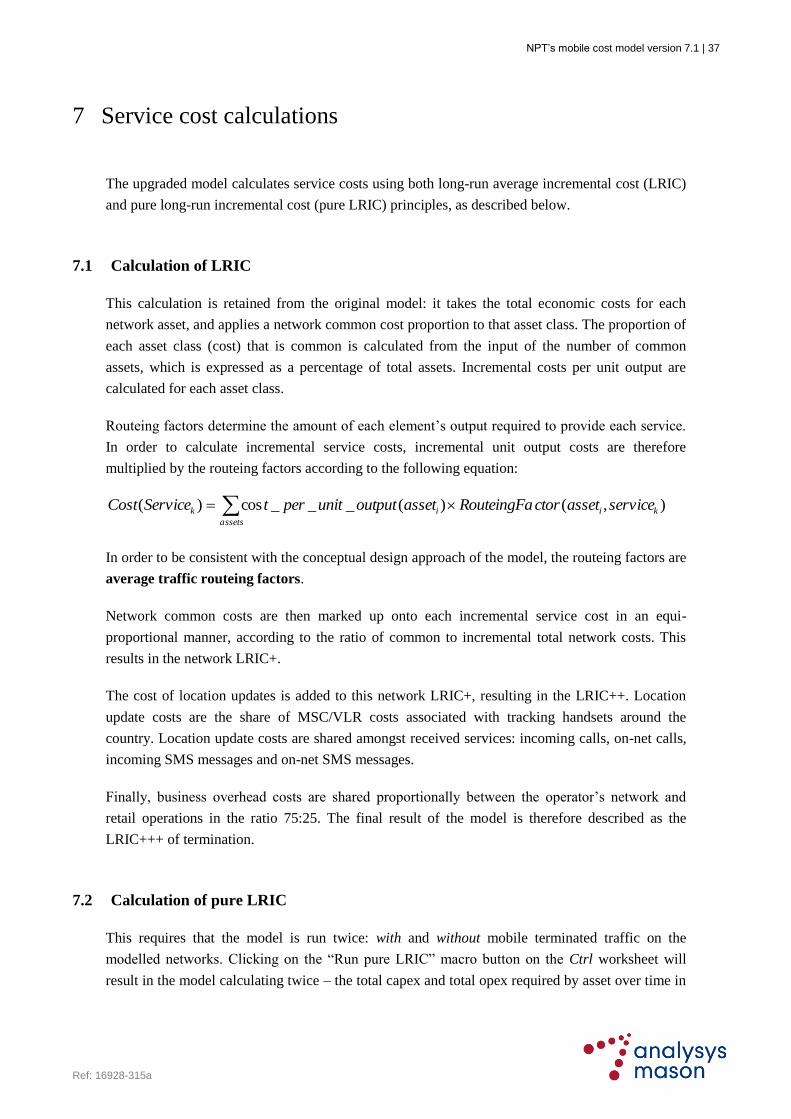
Routeing factors determine the amount of each element‟s output required to provide each service.
In order to calculate incremental service costs, incremental unit output costs are therefore
multiplied by the routeing factors according to the following equation:
),()(___cos)( ki
assets
ik serviceassetctorRouteingFaassetoutputunitpertServiceCost
In order to be consistent with the conceptual design approach of the model, the routeing factors are
average traffic routeing factors.
Network common costs are then marked up onto each incremental service cost in an equi-
proportional manner, according to the ratio of common to incremental total network costs. This
results in the network LRIC+.
The cost of location updates is added to this network LRIC+, resulting in the LRIC++. Location
update costs are the share of MSC/VLR costs associated with tracking handsets around the
country. Location update costs are shared amongst received services: incoming calls, on-net calls,
incoming SMS messages and on-net SMS messages.
Finally, business overhead costs are shared proportionally between the operator‟s network and
retail operations in the ratio 75:25. The final result of the model is therefore described as the
LRIC+++ of termination.
7.2 Calculation of pure LRIC
This requires that the model is run twice: with and without mobile terminated traffic on the
modelled networks. Clicking on the “Run pure LRIC” macro button on the Ctrl worksheet will
result in the model calculating twice – the total capex and total opex required by asset over time in
NPT’s mobile cost model version 7.1 | 38
Ref: 16928-315a
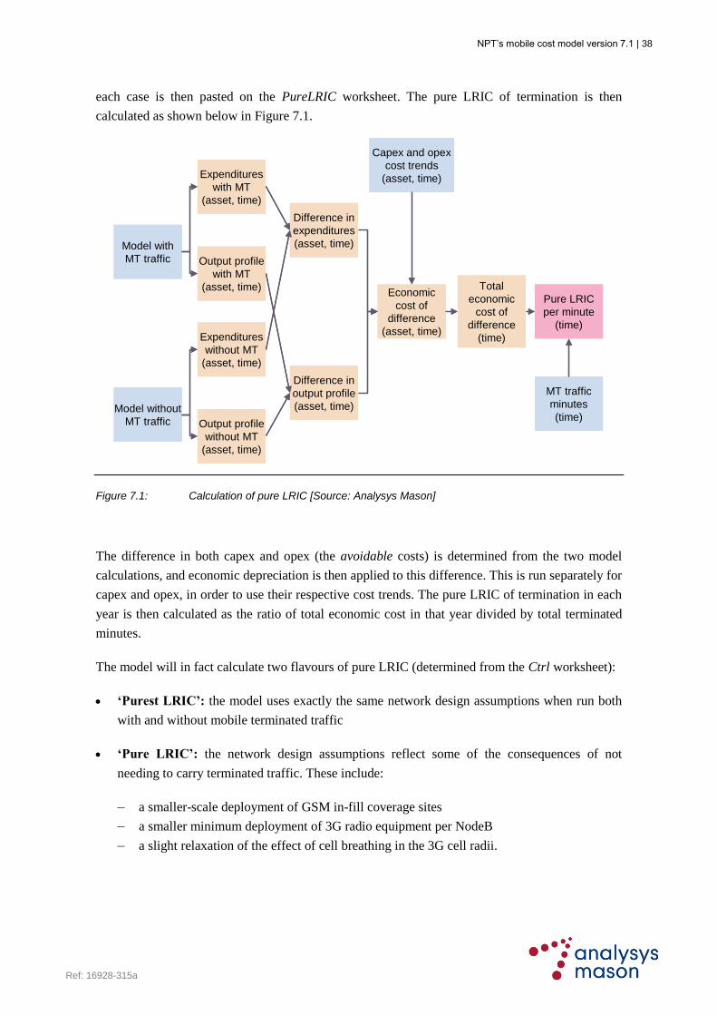
each case is then pasted on the PureLRIC worksheet. The pure LRIC of termination is then
calculated as shown below in Figure 7.1.
Model with
MT traffic
Expenditures
with MT
(asset, time)
Output profile
with MT
(asset, time)
Model without
MT traffic
Expenditures
without MT
(asset, time)
Output profile
without MT
(asset, time)
Difference in
expenditures
(asset, time)
Difference in
output profile
(asset, time)
Economic
cost of
difference
(asset, time)
Pure LRIC
per minute
(time)
MT traffic
minutes
(time)
Capex and opex
cost trends
(asset, time)
Total
economic
cost of
difference
(time)
Figure 7.1: Calculation of pure LRIC [Source: Analysys Mason]
The difference in both capex and opex (the avoidable costs) is determined from the two model
calculations, and economic depreciation is then applied to this difference. This is run separately for
capex and opex, in order to use their respective cost trends. The pure LRIC of termination in each
year is then calculated as the ratio of total economic cost in that year divided by total terminated
minutes.
The model will in fact calculate two flavours of pure LRIC (determined from the Ctrl worksheet):
„Purest LRIC‟: the model uses exactly the same network design assumptions when run both
with and without mobile terminated traffic
„Pure LRIC‟: the network design assumptions reflect some of the consequences of not
needing to carry terminated traffic. These include:
– a smaller-scale deployment of GSM in-fill coverage sites
– a smaller minimum deployment of 3G radio equipment per NodeB
– a slight relaxation of the effect of cell breathing in the 3G cell radii.
NPT’s mobile cost model version 7.1 | 39
Ref: 16928-315a
7.3 2G and 3G allocations
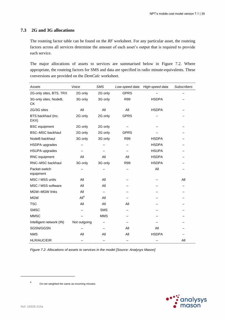
The routeing factor table can be found on the RF worksheet. For any particular asset, the routeing
factors across all services determine the amount of each asset‟s output that is required to provide
each service.
The major allocations of assets to services are summarised below in Figure 7.2. Where
appropriate, the routeing factors for SMS and data are specified in radio minute-equivalents. These
conversions are provided on the DemCalc worksheet.
Assets Voice SMS Low-speed data High-speed data Subscribers
2G-only sites, BTS, TRX 2G only 2G only GPRS – –
3G-only sites, NodeB,
CK
3G only 3G only R99 HSDPA –
2G/3G sites All All All HSDPA –
BTS backhaul (inc.
DXX)
2G only 2G only GPRS – –
BSC equipment 2G only 2G only – – –
BSC–MSC backhaul 2G only 2G only GPRS – –
NodeB backhaul 3G only 3G only R99 HSDPA –
HSDPA upgrades – – – HSDPA –
HSUPA upgrades – – – HSUPA –
RNC equipment All All All HSDPA –
RNC–MSC backhaul 3G only 3G only R99 HSDPA –
Packet-switch
equipment
– – – All –
MSC / MSS units All All – – All
MSC / MSS software All All – – –
MGW–MGW links All – – – –
MGW All4 All – – –
TSC All All All – –
SMSC – SMS – – –
MMSC – MMS – – –
Intelligent network (IN) Not outgoing – – – –
SGSN/GGSN – – All All –
NMS All All All HSDPA –
HLR/AUC/EIR – – – – All
Figure 7.2: Allocations of assets to services in the model [Source: Analysys Mason]
4 On-net weighted the same as incoming minutes
NPT’s mobile cost model version 7.1 | A–1
Ref: 16928-315a
Annex A: Network design algorithms
This section details the algorithms used to build up a network based on the modelled demand
described in Section 3.
A.1 GSM technologies
A.1.1 Radio network: site coverage requirement
In Norway, GSM900MHz spectrum is used for coverage purposes. EGSM channels can be added
to the number of available GSM900MHz channels. To satisfy the coverage requirements, the
number of sites deployed has to be able to provide coverage for a certain area defined by Fylke.
The inputs to the coverage sites calculations are:
total area covered by the mobile operator, by Fylke, for coverage and for infill purposes
year in which wide-area coverage site deployment is completed
year in which infill coverage is completed
cell radii for wide-area coverage for each Fylke
cell radii for infill purposes for each Fylke.
The model allows for additional future coverage to be modelled. The inputs to the future coverage
calculation are:
forecast additional coverage + infill for each Fylke (these are subsequently modelled as
incremental coverage and infill, on the basis of up to 80% area of a Fylke covered by wide-
area coverage, with the remainder deployed as infill)
the year in which the forecast additional coverage + infill is to be achieved
the degree to which the infill coverage signal strength has changed from 2006 to 2008.
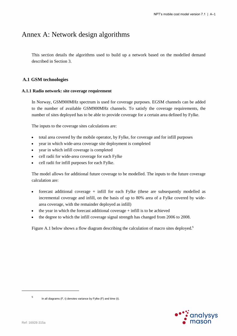
Figure A.1 below shows a flow diagram describing the calculation of macro sites deployed.5
5 In all diagrams (F, t) denotes variance by Fylke (F) and time (t).

NPT’s mobile cost model version 7.1 | A–2
Ref: 16928-315a
Land area km2 (F)% area for coverage
(excluding infill) (F,t)
Coverage area km2 (F,t)
Coverage cell radius for
a given dBm network
quality (F)
Area of site for Coverage
km2 (F)
Hexagonal factor
Number of sites for
coverage (F,t)
Land area km2 (F)% area for infill
(excluding infill) (F,t)
Infill area km2 (F,t)
Infill cell radius for a
given dBm network
quality (F)
Area of site for Infill km2
(F)
Hexagonal factor
Number of sites for infill
(F,t)
Total number of
coverage sites (F,t)
Wide area repeaters per
coverage site (t)Wide area repeaters (t)
Tunnel repeaters (t) Tunnel repeaters (t)
Figure A.1: 900MHz coverage network design [Source: Analysys Mason]
From the site radius, the area covered for a site in a given Fylke is calculated. The total area
covered for the Fylke is divided by this site area to determine the number of sites for coverage that
are deployed. Similarly the number of sites required for infill purposes is calculated.
The number of wide-area repeaters is calculated as a percentage of the total number of coverage
sites in each year. The number of tunnel repeaters is modelled as an explicit input using operator
data.
All coverage sites are assumed to be omni-sectored.
A.1.2 Radio network: site capacity requirement
The calculation of the number of additional sites required for capacity purposes involves the
following steps:
1. Calculation of the capacity provided by the coverage sites

NPT’s mobile cost model version 7.1 | A–3
Ref: 16928-315a
2. Calculation of the capacity provided by sectorising coverage sites, up to a realistic
sectorisation limit
3. Calculation of the capacity provided by overlaying coverage sites with DCS1800MHz
spectrum (if available)
4. Calculation of the number of additional sites (including DCS1800MHz overlays, if available)
required to fulfil capacity requirements.
Step 1: Capacity provided by the coverage network
The calculation of the BHE capacity provided by the sites deployed for coverage purposes is
shown in Figure A.2.
Number of sites for
coverage (F,t)
Omni-sectors for
coverage
Voice radio BHE (F,t)
900MHz channels (t) Maximum reuse factor
900MHz spectral limit to
TRX/sector (t)
Physical BTS limit to
TRX/sector
Capacity of 900MHz
sector, channels (t)
Capacity of 900MHz
sector, BHE, before
utilisation allowance (t)
Radio blocking
probability (2%)
Exclusion of 1 channel
for GPRS reservation
Additional BHE which
must be supported by
sectorisation/DCS (F,t)
Capacity of coverage
sites (F,t)
Binding limit to
TRX/sector (t)
Maximum utilisation of
TRX erlang capacity
Maximum utilisation of
BTS TRX capacity
Effective capacity of
900MHz sector, BHE, (t)
Figure A.2: Calculation of
the BHE capacity
provided by the coverage
network [Source:
Analysys Mason]
Before the capacity requirements of the network are calculated, the Erlang capacity for a given
sector is determined. The inputs to this calculation are the availability of spectrum, the spectrum
re-use factor and the physical BTS capacity.
The spectral capacity is the number of transceivers that can be deployed per sector given a certain
maximum spectrum re-use factor. The lesser of the physical capacity and the spectral capacity of a
sector is the applied capacity.
The sector capacity in Erlangs is obtained using the Erlang B conversion table. At this stage, one
channel of the 900MHz layer is reserved for GPRS. An allowance is made for less than 100% of

NPT’s mobile cost model version 7.1 | A–4
Ref: 16928-315a
the BTS and TRX capacity in the calculation of the effective capacity of each 900MHz sector.
BTS underutilisation occurs because it is not possible to deploy the full physical TRX complement
in every BTS, since BHE demand does not uniformly exist at a small number of sites. TRX
underutilisation occurs because the peak loading of each cell at its busy hour is greater than the
network average busy hour (to take this into account, an average to peak BHE loading of 150% is
used in the calculation of the TRX utilisation, accounting for the fact that the cell busy hour is
50% greater than the network busy hour)6, and because BHE demand does not uniformly occur in
a certain number of sectors.
Given the fact that all coverage sites are assumed to be omni-sectored, the total capacity provided
by the coverage sites is calculated. The BHE traffic is split by Fylke according to operator data to
generate the volume of BHE traffic which must be supported by coverage, sectorisation or through
the overlay with DCS1800MHz sites.
Step 2: Calculation of the capacity provided by sectorising coverage sites
Both Telenor and Netcom provided data with which to calculate the average number of sectors per
capacity site. Using the Erlang capacity of a 900MHz sector, the total Erlang capacity provided by
sectorising the coverage sites, up to the practical sectorisation limit, is calculated. Using the
difference between the additional BHE traffic requirement and the capacity that can be provided
through sectorisation, the number of additional sectors required by Fylke over time and the
number of additional BHE that must be satisfied by overlaying the sectorised coverage sites with
DCS1800MHz spectrum is calculated.
6 The magnitude of this effect being confirmed by the operators’ submissions.

NPT’s mobile cost model version 7.1 | A–5
Ref: 16928-315a
Additional BHE which
must be supported by
sectorisation/DCS (F,t)
% sectorisation in full
network of 1, 2 and 3
sectors
Average number of
sectors per capacity site
Average number of
sectors per sectorised
site over coverage omni
Number of sites for
coverage (F,t)
BHE satisfied (F,t)
Effective capacity of
900MHz sector, BHE, (t)
Additional 900MHz
capacity, BHE (t)
Additional BHE which
must be satisfied by
DCS or more sites (F,t)
Number of additional
sectors required (F,t)
Number of sectorised
sites required (F,t)
Figure A.3: Calculation of
the capacity provided by
sectorising coverage site
[Source: Analysys
Mason]
Step 3: Calculation of the capacity provided by overlaying coverage sites with DCS1800MHz
spectrum
Coverage sites that have been sectorised can be further augmented with DCS capacity, if these
channels are available, and where demand exists in excess of that supported by sectorisation. We
assume that omni-sites remaining for coverage are not overlaid with DCS capacity since they are
not located at the hotspots of demand.
The sectorisation proportion of DCS overlays is combined with the DCS per-sector capacity
(calculated as before from DCS spectrum, re-use, physical constraints and utilisation parameters).
This allows the number of DCS overlays to be calculated according to the BHE demand that must
be supported. If all sectorised coverage sites are augmented with DCS overlays, then excess BHE
must be supported by new site deployments.
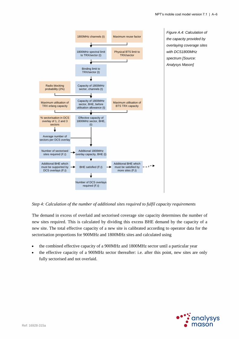
NPT’s mobile cost model version 7.1 | A–6
Ref: 16928-315a
% sectorisation in DCS
overlay of 1, 2 and 3
sectors
Average number of
sectors per DCS overlay
Effective capacity of
1800MHz sector, BHE,
(t)
1800MHz channels (t) Maximum reuse factor
1800MHz spectral limit
to TRX/sector (t)
Physical BTS limit to
TRX/sector
Capacity of 1800MHz
sector, channels (t)
Capacity of 1800MHz
sector, BHE, before
utilisation allowance (t)
Radio blocking
probability (2%)
Binding limit to
TRX/sector (t)
Maximum utilisation of
TRX erlang capacity
Maximum utilisation of
BTS TRX capacity
Number of sectorised
sites required (F,t)
Additional 1800MHz
overlay capacity, BHE (t)
Additional BHE which
must be supported by
DCS overlays (F,t)
BHE satisfied (F,t)
Additional BHE which
must be satisfied by
more sites (F,t)
Number of DCS overlays
required (F,t)
Figure A.4: Calculation of
the capacity provided by
overlaying coverage sites
with DCS1800MHz
spectrum [Source:
Analysys Mason]
Step 4: Calculation of the number of additional sites required to fulfil capacity requirements
The demand in excess of overlaid and sectorised coverage site capacity determines the number of
new sites required. This is calculated by dividing this excess BHE demand by the capacity of a
new site. The total effective capacity of a new site is calibrated according to operator data for the
sectorisation proportions for 900MHz and 1800MHz sites and calculated using
the combined effective capacity of a 900MHz and 1800MHz sector until a particular year
the effective capacity of a 900MHz sector thereafter: i.e. after this point, new sites are only
fully sectorised and not overlaid.
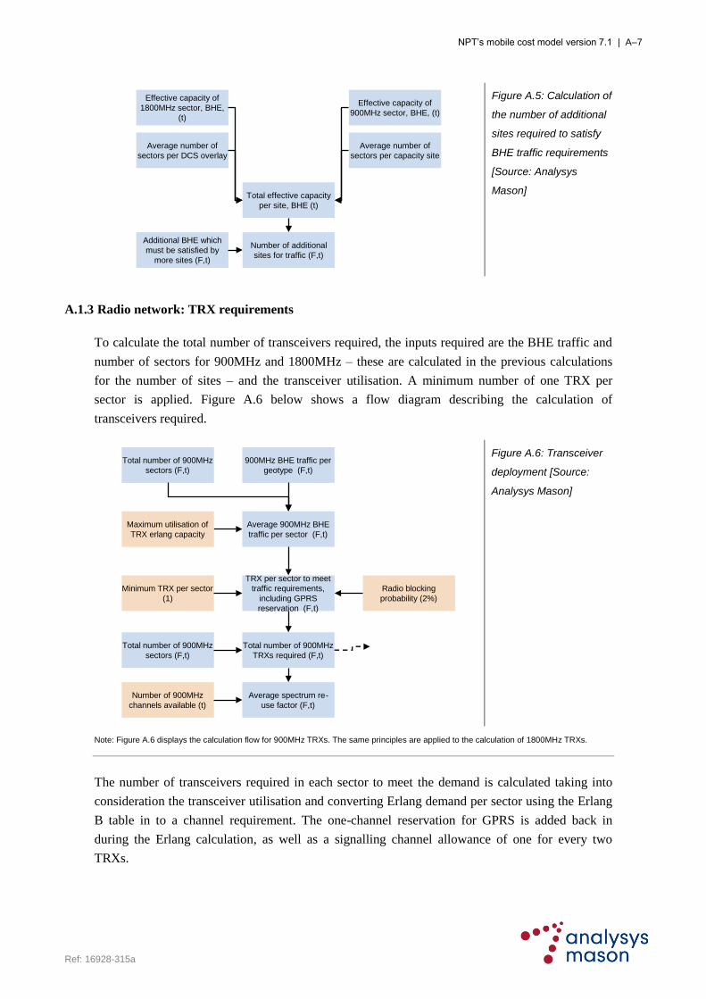
NPT’s mobile cost model version 7.1 | A–7
Ref: 16928-315a
Additional BHE which
must be satisfied by
more sites (F,t)
Average number of
sectors per DCS overlay
Effective capacity of
1800MHz sector, BHE,
(t)
Average number of
sectors per capacity site
Effective capacity of
900MHz sector, BHE, (t)
Total effective capacity
per site, BHE (t)
Number of additional
sites for traffic (F,t)
Figure A.5: Calculation of
the number of additional
sites required to satisfy
BHE traffic requirements
[Source: Analysys
Mason]
A.1.3 Radio network: TRX requirements
To calculate the total number of transceivers required, the inputs required are the BHE traffic and
number of sectors for 900MHz and 1800MHz – these are calculated in the previous calculations
for the number of sites – and the transceiver utilisation. A minimum number of one TRX per
sector is applied. Figure A.6 below shows a flow diagram describing the calculation of
transceivers required.
Total number of 900MHz
sectors (F,t)
900MHz BHE traffic per
geotype (F,t)
Average 900MHz BHE
traffic per sector (F,t)
Radio blocking
probability (2%)
Minimum TRX per sector
(1)
Maximum utilisation of
TRX erlang capacity
TRX per sector to meet
traffic requirements,
including GPRS
reservation (F,t)
Total number of 900MHz
TRXs required (F,t)
Total number of 900MHz
sectors (F,t)
Number of 900MHz
channels available (t)
Average spectrum re-
use factor (F,t)
Figure A.6: Transceiver
deployment [Source:
Analysys Mason]
Note: Figure A.6 displays the calculation flow for 900MHz TRXs. The same principles are applied to the calculation of 1800MHz TRXs.
The number of transceivers required in each sector to meet the demand is calculated taking into
consideration the transceiver utilisation and converting Erlang demand per sector using the Erlang
B table in to a channel requirement. The one-channel reservation for GPRS is added back in
during the Erlang calculation, as well as a signalling channel allowance of one for every two
TRXs.
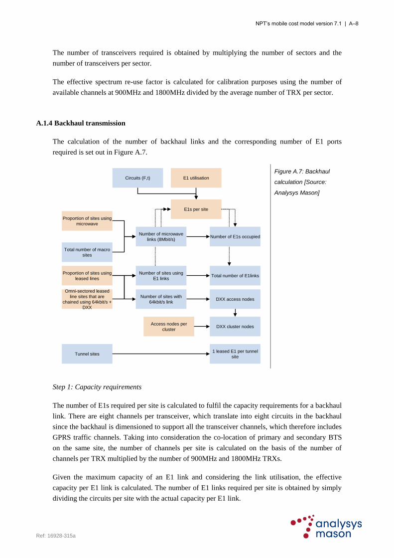
NPT’s mobile cost model version 7.1 | A–8
Ref: 16928-315a
The number of transceivers required is obtained by multiplying the number of sectors and the
number of transceivers per sector.
The effective spectrum re-use factor is calculated for calibration purposes using the number of
available channels at 900MHz and 1800MHz divided by the average number of TRX per sector.
A.1.4 Backhaul transmission
The calculation of the number of backhaul links and the corresponding number of E1 ports
required is set out in Figure A.7.
Circuits (F,t)
Total number of macro
sites
Tunnel sites1 leased E1 per tunnel
site
Proportion of sites using
microwave
Proportion of sites using
leased lines
E1 utilisation
E1s per site
Omni-sectored leased
line sites that are
chained using 64kbit/s +
DXX
Number of sites using
E1 links
Number of sites with
64kbit/s linkDXX access nodes
Number of microwave
links (8Mbit/s)
Total number of E1links
Number of E1s occupied
DXX cluster nodesAccess nodes per
cluster
Figure A.7: Backhaul
calculation [Source:
Analysys Mason]
Step 1: Capacity requirements
The number of E1s required per site is calculated to fulfil the capacity requirements for a backhaul
link. There are eight channels per transceiver, which translate into eight circuits in the backhaul
since the backhaul is dimensioned to support all the transceiver channels, which therefore includes
GPRS traffic channels. Taking into consideration the co-location of primary and secondary BTS
on the same site, the number of channels per site is calculated on the basis of the number of
channels per TRX multiplied by the number of 900MHz and 1800MHz TRXs.
Given the maximum capacity of an E1 link and considering the link utilisation, the effective
capacity per E1 link is calculated. The number of E1 links required per site is obtained by simply
dividing the circuits per site with the actual capacity per E1 link.
NPT’s mobile cost model version 7.1 | A–9
Ref: 16928-315a
Step 2: Backhaul network design algorithms
There are two types of backhaul to be considered in the network: microwave (8Mbit/s links) and
leased line backhaul. The percentage of sites which have microwave backhaul is an input into the
model.
The number of microwave 8Mbit/s backhaul links is set to be a minimum of one per site. The
model allows for more than one 8Mbit/s link per site, though traffic requirements are unlikely to
present such a high load. The number of E1 units occupied in each 8Mbit/s microwave link is
calculated.
The number of sites using leased lines calculated as the difference between the total sites and the
total sites using microwaves. The total number of E1 leased lines required is the multiplication of
total macro sites using leased line and the number of E1 required per site (from Step 1). Where
sites have less than a specified low traffic requirement, a 64kbit/s leased line backhaul may be
used.
DXX access nodes are deployed according for 64kbit/s links, and are modelled to persist in the
network even when the 64kbit/s links are replaced by higher-capacity E1. DXX cluster nodes are
deployed on the basis of n access nodes per cluster node.
Tunnel repeater sites are assumed to use only E1 leased-line backhaul and hence are added to the
leased-line requirement of the macro layer.
A.1.5 BSC deployment
The structure of the BSC deployment algorithm is set out below in Figure A.8.

NPT’s mobile cost model version 7.1 | A–10
Ref: 16928-315a
BSC locations (F,t)
BSC capacity in TRX
Maximum utilisation
TRX (F,t)
TRX mapped to Fylke
(F,t)
TRX per BSC location
(F,t)
Number of BSC required
per location (F,t)
Total number of BSC
(F,t)
Backhaul links, less DXX
access nodes
Number of BSC E1 ports
facing backhaul
MSC-facing E1 ports per
BSC (F,t)BSC-MSC BHE (F,t)
Total number of MSC-
facing BSC E1 ports (t)
Figure A.8: BSC
deployment [Source:
Analysys Mason]
BSC units calculation
The number of BSC units deployed is dependent on the capacity of a BSC, its utilisation and the
total number of transceivers required.
BSC locations by Fylke are used as an input to the model using data from the operators. TRXs are
mapped onto these BSC locations by Fylke, generating the number of TRX per BSC location. The
number of BSC units deployed must be able to accommodate the number of transceivers deployed
(see Section A.1.3). Given a maximum capacity of the BSC in terms of TRX, adjusted for
maximum utilisation, the number of BSCs required per location is calculated.

NPT’s mobile cost model version 7.1 | A–11
Ref: 16928-315a
BSC–MSC links calculation
BSC locations (F,t)
MSC locations (F,t)BSC locations mapped
to MSC locations (F,t)
Remote BSC locations
(F,t)
BSC-MSC BHE (F,t)
BSC-MSC BHE mapped
to Fylke (F,t)
BSC-MSC BHE per
remote BSC location
(F,t)
E1 capacity and
utilisationNumber of E1 links (F,t)
Distance of E1 links (F,t)
Figure A.9: BSC–MSC
remote transmission
[Source: Analysys
Mason]
A proportion of BSCs are designated as „remote‟ (i.e. not co-located with an MSC), and therefore
require physical links to the MSC and are located in a separate building in some distant part of the
network. Remote BSC locations are modelled to be present when the number of BSC locations in
a Fylke is greater than the number of MSC locations in that Fylke (each MSC location logically
has a co-located BSC location). In terms of the actual number of remote BSCs, in a Fylke in which
there are no MSC locations, all BSCs in the Fylke are remote. When there are MSC locations in
the Fylke, it is assumed that there is one remote BSC per remote BSC location.
The traffic transiting through these BSCs is backhauled to the MSC using E1 leased lines. Remote
BSCs require physical BSC–MSC links and the total is calculated from the total number of remote
BSCs and the link capacity required.
The total traffic handled by each remote BSC can be calculated using the total BHE transceiver
traffic. The volume of this BHE traffic is calculated according to the ratio of remote BSCs to total
BSCs in a Fylke. The average BHE traffic handled by each remote BSC is then converted into a
channel requirement using the Erlang table. The number of E1 links is then calculated by dividing
this channel requirement by the capacity of an E1 link, adjusted for maximum utilisation. It should
be noted that the capacity of the BSC–MSC transmission depends on where the transcoder
equipment is located. For remote BSCs, the transcoder is located in the MSC, and so, according to
the GSM standard, has a capacity of 120 circuits.
The distance of these links is also an important output of the model as the backhaul costs involve a
connection charge per link end and a distance-based cost.
The distances between all of the Fylker is specified in the NtwDesBase worksheet according to
straight-line distances between the major conurbations in each Fylke, adjusted for route length
using a multiplier of 1.3 (accounting for the non-straight line nature of networks given topology

NPT’s mobile cost model version 7.1 | A–12
Ref: 16928-315a
constraints). The calculation of the distances of the BSC–MSC links uses this Fylke distance
matrix, in combination with the mapping of BSCs locations onto MSCs locations, which is
performed in the BSCMSC worksheet.
The number of E1 BSC–MSC ports is determined on the basis of the number of BSC–MSC E1
links.
Total outgoing ports for co-located BSCs
Given the total number of co-located BSCs and BHE transceiver traffic, the total number of
outgoing ports for co-located BSCs is calculated. The flow of calculation for co-located BSC ports
is similar to that shown in Figure A.9 except the transcoder is assumed to be in the BSC (therefore
E1 capacity is 30 channels) and the distance of co-located links is not modelled.
Incoming and outgoing ports
The incoming ports to the BSC are ports facing the BTS while the outgoing ports are ports facing
the MSC. Figure A.10 below shows the constituents of the incoming and outgoing ports.
Total E1 incoming ports
Number of E1 for remote
BSC-MSC links
Incoming ports Outgoing ports
Number of occupied E1
units of 8Mbit/s backhaul
Number of leased line
E1 links
Number of DXX cluster
nodes
Number of E1 for co-
located BSC-MSC links
Total E1 outgoing ports
Figure A.10: Total incoming and outgoing ports for BSC [Source: Analysys Mason]
The total number of E1 incoming ports into BSC is the sum of microwave and leased line
backhaul links while the total outgoing ports is the sum of the total number of E1 for both remote
and co-located BSCs.
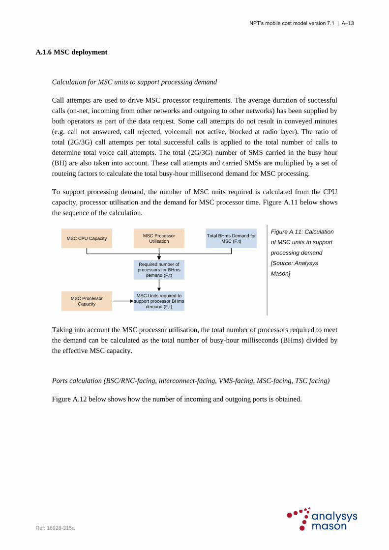
NPT’s mobile cost model version 7.1 | A–13
Ref: 16928-315a
A.1.6 MSC deployment
Calculation for MSC units to support processing demand
Call attempts are used to drive MSC processor requirements. The average duration of successful
calls (on-net, incoming from other networks and outgoing to other networks) has been supplied by
both operators as part of the data request. Some call attempts do not result in conveyed minutes
(e.g. call not answered, call rejected, voicemail not active, blocked at radio layer). The ratio of
total (2G/3G) call attempts per total successful calls is applied to the total number of calls to
determine total voice call attempts. The total (2G/3G) number of SMS carried in the busy hour
(BH) are also taken into account. These call attempts and carried SMSs are multiplied by a set of
routeing factors to calculate the total busy-hour millisecond demand for MSC processing.
To support processing demand, the number of MSC units required is calculated from the CPU
capacity, processor utilisation and the demand for MSC processor time. Figure A.11 below shows
the sequence of the calculation.
MSC CPU CapacityMSC Processor
Utilisation
Total BHms Demand for
MSC (F,t)
Required number of
processors for BHms
demand (F,t)
MSC Processor
Capacity
MSC Units required to
support processor BHms
demand (F,t)
Figure A.11: Calculation
of MSC units to support
processing demand
[Source: Analysys
Mason]
Taking into account the MSC processor utilisation, the total number of processors required to meet
the demand can be calculated as the total number of busy-hour milliseconds (BHms) divided by
the effective MSC capacity.
Ports calculation (BSC/RNC-facing, interconnect-facing, VMS-facing, MSC-facing, TSC facing)
Figure A.12 below shows how the number of incoming and outgoing ports is obtained.

NPT’s mobile cost model version 7.1 | A–14
Ref: 16928-315a
MSC locations (t)
Interconnection BHE
traffic (t)
Interconnection traffic
per MSC location
Erlang table channel
calculation
Interconnection traffic
per MSC location
(channels) (t)
Interconnection port
utilisation
E1 capacity (circuits)
Interconnection ports per
location (E1s) (t)
MSC locations (t)
Number of
interconnection-facing
E1 ports required (t)
Interconnect infrastructure VMS ports
Voicemail BHE traffic (t)
Erlang table channel
calculation
Voicemail traffic
(channels) (t)
Port utilisation
E1 capacity (circuits)
VMS ports (E1s) (t)
Incoming ports
Total number of outgoing
E1 ports from BSCs (t)
Total number of
incoming E1 ports from
BSCs (t)
Ports x2 for redundancy
De-multiplexed outgoing
STM1 ports from
RNCs (t)
Figure A.12: Without a transit layer – calculation of MSC ports: BSC-facing ports, interconnect-facing
ports, VMS-facing ports [Source: Analysys Mason]
The total number of incoming ports in the MSC is simply taken as the total number of E1 outgoing
ports from the BSC, as well as the total RNC-facing ports de-multiplexed from STM–1.
The total number of outgoing ports comprises the number of interconnect-facing ports required,
the number of VMS-facing ports required (both shown conceptually in Figure A.12) and the
number of inter-switch ports required (shown in Figure A.13).
For the interconnection infrastructure, the total number of interconnect-facing ports required to
meet demand is obtained by dividing the interconnection BHE traffic at each MSC location (as a
channel requirement) with the actual E1 capacity of the port. Full redundancy is accounted for by
doubling the number of ports at each MSC location.
The model accounts for two network states when calculating the number of MSC inter-switch
ports (and links): without a transit layer, and with a transit layer. These are presented separately
below.
Without a transit layer
The calculation of the number of inter-switch ports is detailed below. This calculation takes into
account the Intra-Oslo backbone ring, which exists when there is more than one MSC location
within Oslo.

NPT’s mobile cost model version 7.1 | A–15
Ref: 16928-315a
Mapping of BSCs onto
MSCs (F, t)
Traffic handled by a
particular BSC Fylke (F,
t)
BHE per MSC Fylke (F,
t)
Proportion of BHE traffic
that are into/out of Oslo
(t)
BHE traffic per route (t)
Backbone infrastructure (into Oslo)
Interswitch BHE traffic (t)
VMS BHE traffic (t)Number of routes into
Oslo (t)
Number of MSC
locations outside of Oslo
(t)
Channels per route (t)Erlang table channel
calculation
E1 capacity (circuits) Ports utilisationNumber of E1 per route
(t)
Number of routes into
Oslo (t)
Number of E1 links/ports
outside of Oslo (t)E1 x2 for redundancy
Number of E1 ports
inside of Oslo (t)
BHE traffic per route (t)
Backbone infrastructure (intra Oslo)
Intra-Oslo ring present if
MSC locations in Oslo
>1 (t)
Channels per route (t)
Number of E1 per route
(t)
Number of E1 links/ports
one end in Oslo (t)
Number of E1 ports
other end in Oslo (t)
BHE traffic on Oslo ring
(t)
Number of MSC
locations in Oslo (t)
Number of logical routes
on ring (t)
Erlang table channel
calculation
E1 capacity (circuits)
Number of routes into
Oslo (t)
Figure A.13: Without a transit layer – calculation of the number of inter-switch ports
[Source: Analysys Mason]
The proportion of inter-switch and VMS traffic carried over the logically fully-meshed intra-Oslo
ring is used to dimension the number of E1 links and ports within the Oslo ring, with the
remaining traffic being carried from the MSC locations in the other Fylker to Oslo. This traffic
dimensions the number of E1 links and ports required outside of Oslo (on MSCs all facing Oslo)
and inside of Oslo (on Oslo MSCs facing the MSCs in the other Fylker). Full E1 redundancy is
provided.
With a transit layer
When a transit layer is deployed (modelled to occur when TSCs are present in more than one
Fylke), the transit layer performs the same function as the Oslo core in the non-transit network.
This is shown below in Figure A.14.

NPT’s mobile cost model version 7.1 | A–16
Ref: 16928-315a
BHE per MSC Fylke (F,
t)
Proportion of BHE traffic
that are into/out of
Transit layer (t)
BHE traffic per route (t)
Into Transit Layer
Interswitch BHE traffic (t)
VMS BHE traffic (t)Number of routes into
Transit layer (t)
Number of MSC
locations outside of
Transit layer (t)
Channels per route (t)Erlang table channel
calculation
E1 capacity (circuits) Ports utilisationNumber of E1 per route
(t)
Number of routes into
Transit layer (t)
Number of E1 links/ports
into Transit layer (t)E1 x2 for redundancy
BHE traffic per route (t)
Other MSC within Transit Layer
Channels per route (t)
Number of E1 per route
(t)
Number of E1 links/ports
within transit layer (t)
Erlang table channel
calculation
E1 capacity (circuits)
Number of MSC within
Transit layer (t)
TSC locations (F, t)BHE in Fylke which are
Non-TSC Fylke (F, t)
Number of MSC inside
Transit layer (t)
Figure A.14: With a transit layer – calculation of the number of inter-switch ports to the transit layer
[Source: Analysys Mason]
BHE traffic is proportioned according to whether or not the MSC lies within a Fylke that contains
a TSC. The number of outgoing ports to the transit layer is dimensioned according to the same
principles as outlined in the non-transit layer case.
Calculation for MSC units to support port demand
MSC support for ports is based on the total incoming and outgoing ports for the MSC base. Figure
A.15 below shows the calculation flow to obtain the number of MSC units required.

NPT’s mobile cost model version 7.1 | A–17
Ref: 16928-315a
Total number of
incoming E1 ports from
BSCs (t)
Total number of outgoing
E1 ports to MSC/Transit
layer (t)
Number of
interconnection-facing
E1 ports required (t)
VMS ports (E1s) (t)
MSC port capacity
MSC port utilisation
Number of MSC units
required to support ports
demand(t)
Total number of ports (t)
De-multiplexed STM-1
incoming ports from
RNCs (t)
Figure A.15: Calculation
of MSC units to support
port demand [Source:
Analysys Mason]
The total number of ports is the sum of all incoming and outgoing ports from the MSC. Dividing
this total number with the effective port capacity of an MSC gives the number of MSC units to
meet the port demand.
A.1.7 Transit layer deployment
The deployment of a transit layer is based upon the number of TSC locations provided by the
operators. A transit layer is modelled to be present when more than one Fylke has a TSC deployed.
One TSC per location is modelled. TSC ports are not explicitly modelled, and are assumed to be
included in the TSC unit cost.
A.1.8 Backbone transmission
There are two backbone network design options:
without transit layer: fully redundant links into Oslo, plus Oslo ring
with transit layer: fully redundant links in to the transit layer, plus transit mesh.
Network without transit layer
The inter-switch transmission links for a network design without a transit layer are calculated
based on the number of switching sites deployed. Figure A.16 below shows how the calculations
are carried out.

NPT’s mobile cost model version 7.1 | A–18
Ref: 16928-315a
Number of E1 per route
(into Oslo) (t)
Capacity of a backbone
link
Backbone utilisation
Number of STM-1 per
route (t)
Number of routes into
Oslo (t)
Total STM-1 links into
Oslo (t)
STM-1 x2 for
redundancy
Distance of STM-1
routes to Oslo
Total STM-1 km length
(links into Oslo) (t)
Figure A.16: MSC–MSC
links for a network
without transit layer
[Source: Analysys
Mason]
The diagram shows the calculation flow for links into Oslo. This same calculation is used for the
total STM–1 links and link lengths for the intra-Oslo MSC–MSC ring.
Backbone links are modelled as STM–1 (155Mbit/s). These can accommodate 63 E1 links, subject
to a maximum utilisation percentage.
The number of E1s per route is calculated in the port calculation. The corresponding number of
STM–1 units per route is then calculated taking into account the fact that full redundancy is
provided on each link. Multiplying by the number of routes gives the total number of STM–1 links
into/within Oslo. The distance of the MSC–MSC links into Oslo is based on the straight-line
distance (adjusted by a factor of 1.3 to take into account the non-straight line nature of the routes
due to topology constraints) from each Fylke containing an MSC location to Oslo. The link lengths
for MSC–MSC links within Oslo are assumed to be 3km.
Network with transit layer
The calculation of MSC–TSC links is based on the same principles as outlined above for MSC–
MSC links, with the exception that the links are from the MSC location to the nearest TSC
location (with redundancy). This calculation was outlined for the port requirement calculation.
Figure A.17 below shows the calculation for the TSC–TSC links.

NPT’s mobile cost model version 7.1 | A–19
Ref: 16928-315a
Mapping of BSCs onto
MSCs (F, t)
Interswitch BHE traffic +
VMS BHE traffic (t)
BHE on Transit layer (t)
Channels per route (t)
Number of E1 per route
(t)
Number of E1 links/ports
one end in Transit layer
(t)
Number of E1 ports
other end in Transit layer
(t)
BHE traffic per route (t)
Ports utilisation
E1 x2 for redundancy
Erlang table channel
calculation
E1 capacity (circuits)
Number of routes (fully
meshed) (t)
% national minutes
transmitted across
transit layer
Number of transit
locations (t)
Number of routes (fully
meshed) (t)
Figure A.17: Total TSC–
TSC links for a network
with transit layers
[Source: Analysys
Mason]
The number of TSC–TSC links is calculated directly using the number of transit switches, S, with
the formula below:
l = S (S-1) / 2
The subsequent algorithms for the total number of STM–1 for the TSC–TSC backbone links are
similar to that carried out for the MSC–TSC links.
The transit link distances are based upon an average link distance calculated from the total distance
between each of the Fylker that contain a TSC location. However, TSC–TSC links are assumed to
be carried on a physical ring rather than fully-meshed links, therefore, the length of TSC–TSC
links is estimated according to national TSC locations including an Oslo ring if more than one
TSC exists in Oslo.
Overall inter-switch transmission links requirements
In summary, when there is no transit layer, the total number of STM–1 links will equal the total
number of MSC–MSC links in Oslo plus the total number of MSC–MSC links into Oslo. When
there is a transit layer present, the total number of STM–1 links will equal the total MSC–TSC
links into the transit layer plus the total number of STM–1 TSC–TSC links.
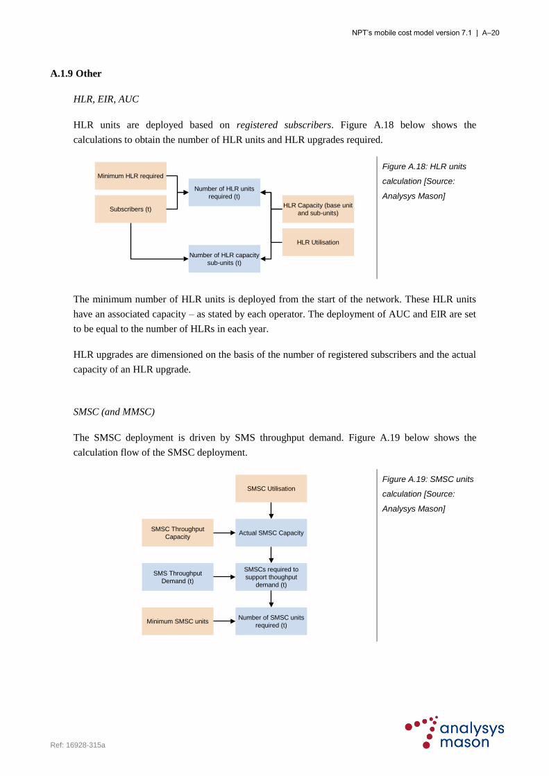
NPT’s mobile cost model version 7.1 | A–20
Ref: 16928-315a
A.1.9 Other
HLR, EIR, AUC
HLR units are deployed based on registered subscribers. Figure A.18 below shows the
calculations to obtain the number of HLR units and HLR upgrades required.
Minimum HLR required
Number of HLR units
required (t)
HLR Capacity (base unit
and sub-units)
HLR Utilisation
Subscribers (t)
Number of HLR capacity
sub-units (t)
Figure A.18: HLR units
calculation [Source:
Analysys Mason]
The minimum number of HLR units is deployed from the start of the network. These HLR units
have an associated capacity – as stated by each operator. The deployment of AUC and EIR are set
to be equal to the number of HLRs in each year.
HLR upgrades are dimensioned on the basis of the number of registered subscribers and the actual
capacity of an HLR upgrade.
SMSC (and MMSC)
The SMSC deployment is driven by SMS throughput demand. Figure A.19 below shows the
calculation flow of the SMSC deployment.
SMSC Throughput
Capacity
SMSC Utilisation
Actual SMSC Capacity
SMS Throughput
Demand (t)
SMSCs required to
support thoughput
demand (t)
Minimum SMSC unitsNumber of SMSC units
required (t)
Figure A.19: SMSC units
calculation [Source:
Analysys Mason]

NPT’s mobile cost model version 7.1 | A–21
Ref: 16928-315a
Dividing the SMS throughput demand by the actual SMSC capacity gives the number of SMSCs
required to support this throughput demand. The number of SMSC units deployed is the higher of
either the SMSCs required to support demand or the minimum SMSC units threshold.
MMSC deployment is driven by MMS throughput demand in an analogous fashion.
GPRS infrastructure
There are three GPRS infrastructures deployed, namely:
PCU
SGSN
GGSN.
One PCU unit is installed to control a defined number of radio sites.
Figure A.20 below shows the calculations for SGSN and GGSN deployment.
SGSN/GGSN Capacity
SGSN/GGSN Utilisation
Actual SGSN/GGSN
Capacity
Connected
subscribers/active PDP
contexts in the busy hour
(t)
SGSNs/GGSNs required
to support BH connected
subs/PDP contexts (t)
Minimum SGSN/GGSN
units
Number of SGSN/GGSN
units required (t)
Figure A.20: SGSN and
GGSN units calculation
[Source: Analysys
Mason]
The calculations for both SGSN and GGSN deployment are similar. SGSN deployment is driven
by the number of simultaneously attached subscribers in the busy hour while GGSN deployment is
driven by active PDP contexts made in the busy hour.
Dividing their respective demand by the actual SGSN and GGSN capacity gives the total number
of units that are required to meet the demand requirements. The number of SGSN and GGSN
deployed is the higher of either the number of units calculated to meet demand or the minimum
threshold units.
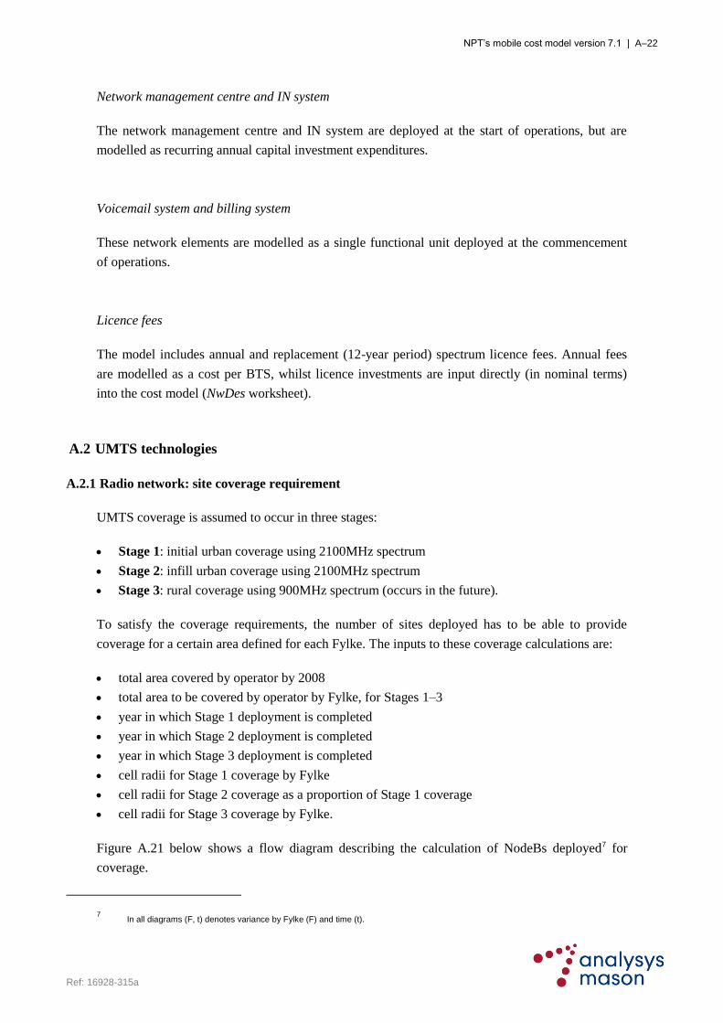
NPT’s mobile cost model version 7.1 | A–22
Ref: 16928-315a
Network management centre and IN system
The network management centre and IN system are deployed at the start of operations, but are
modelled as recurring annual capital investment expenditures.
Voicemail system and billing system
These network elements are modelled as a single functional unit deployed at the commencement
of operations.
Licence fees
The model includes annual and replacement (12-year period) spectrum licence fees. Annual fees
are modelled as a cost per BTS, whilst licence investments are input directly (in nominal terms)
into the cost model (NwDes worksheet).
A.2 UMTS technologies
A.2.1 Radio network: site coverage requirement
UMTS coverage is assumed to occur in three stages:
Stage 1: initial urban coverage using 2100MHz spectrum
Stage 2: infill urban coverage using 2100MHz spectrum
Stage 3: rural coverage using 900MHz spectrum (occurs in the future).
To satisfy the coverage requirements, the number of sites deployed has to be able to provide
coverage for a certain area defined for each Fylke. The inputs to these coverage calculations are:
total area covered by operator by 2008
total area to be covered by operator by Fylke, for Stages 1–3
year in which Stage 1 deployment is completed
year in which Stage 2 deployment is completed
year in which Stage 3 deployment is completed
cell radii for Stage 1 coverage by Fylke
cell radii for Stage 2 coverage as a proportion of Stage 1 coverage
cell radii for Stage 3 coverage by Fylke.
Figure A.21 below shows a flow diagram describing the calculation of NodeBs deployed7 for
coverage.
7 In all diagrams (F, t) denotes variance by Fylke (F) and time (t).

NPT’s mobile cost model version 7.1 | A–23
Ref: 16928-315a
Land area km2 (F)% area for coverage (in
Stage 1) (F,t)
Coverage area in Stage
1 in km2 (F,t)
Stage 1 coverage cell
radius for a given dBm
network quality (F)
Area of site for coverage
in Stage 1 in km2 (F)
Hexagonal factor
Number of sites for
coverage in stage 1 (F,t)
Land area km2 (F)% area for coverage (in
Stage 2) (F,t)
Coverage area in Stage
2 in km2 (F,t)
Stage 2 coverage cell
radius for a given dBm
network quality (F)
Area of site for for
coverage in Stage 2 in
km2 (F)
Number of sites for
Stage 2 coverage (F,t)
Total number of
2100MHz sites for
coverage (F,t)
Wide area repeaters per
coverage site (t)Wide area repeaters (t)
Tunnel repeaters (t) Tunnel repeaters (t)
Land area km2 (F)% area for coverage (in
Stage 3) (F,t)
Coverage area in Stage
3 in km2 (F,t)
Stage 3 coverage cell
radius for a given dBm
network quality (F)
Area of site for for
coverage in Stage 3 in
km2 (F)
Number of sites for
Stage 3 coverage (F,t)
Total number of 900MHz
sites for coverage (F,t)
Total number of sites for
coverage (F,t)
Figure A.21: UMTS coverage network design [Source: Analysys Mason]
NodeB requirements are calculated separately for Stages 1–3. For each of these stages, the NodeB
radius is used to derive the area covered by a NodeB in a given Fylke. The total area covered
within the Fylke is divided by this NodeB area to determine the number of NodeBs for coverage.
The total requirements across all three stages is then calculated for each year by Fylke.
The number of wide-area repeaters is calculated as a percentage of the total number of coverage
NodeBs in each year. The number of tunnel repeaters is modelled as an explicit input using
operator data.
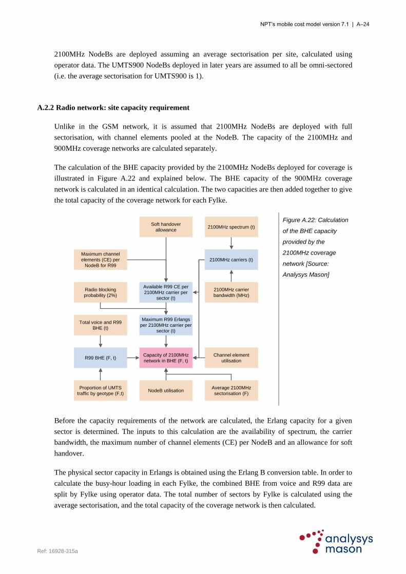
NPT’s mobile cost model version 7.1 | A–24
Ref: 16928-315a
2100MHz NodeBs are deployed assuming an average sectorisation per site, calculated using
operator data. The UMTS900 NodeBs deployed in later years are assumed to all be omni-sectored
(i.e. the average sectorisation for UMTS900 is 1).
A.2.2 Radio network: site capacity requirement
Unlike in the GSM network, it is assumed that 2100MHz NodeBs are deployed with full
sectorisation, with channel elements pooled at the NodeB. The capacity of the 2100MHz and
900MHz coverage networks are calculated separately.
The calculation of the BHE capacity provided by the 2100MHz NodeBs deployed for coverage is
illustrated in Figure A.22 and explained below. The BHE capacity of the 900MHz coverage
network is calculated in an identical calculation. The two capacities are then added together to give
the total capacity of the coverage network for each Fylke.
2100MHz spectrum (t)
2100MHz carrier
bandwidth (MHz)
2100MHz carriers (t)
Soft handover
allowance
Maximum R99 Erlangs
per 2100MHz carrier per
sector (t)
Radio blocking
probability (2%)
Available R99 CE per
2100MHz carrier per
sector (t)
Maximum channel
elements (CE) per
NodeB for R99
Total voice and R99
BHE (t)
Proportion of UMTS
traffic by geotype (F,t)
R99 BHE (F, t)Capacity of 2100MHz
network in BHE (F, t)
Average 2100MHz
sectorisation (F)
Channel element
utilisation
NodeB utilisation
Figure A.22: Calculation
of the BHE capacity
provided by the
2100MHz coverage
network [Source:
Analysys Mason]
Before the capacity requirements of the network are calculated, the Erlang capacity for a given
sector is determined. The inputs to this calculation are the availability of spectrum, the carrier
bandwidth, the maximum number of channel elements (CE) per NodeB and an allowance for soft
handover.
The physical sector capacity in Erlangs is obtained using the Erlang B conversion table. In order to
calculate the busy-hour loading in each Fylke, the combined BHE from voice and R99 data are
split by Fylke using operator data. The total number of sectors by Fylke is calculated using the
average sectorisation, and the total capacity of the coverage network is then calculated.

NPT’s mobile cost model version 7.1 | A–25
Ref: 16928-315a
An allowance is made for less than 100% of the NodeB and CE capacity being utilised. NodeB
underutilisation occurs because it is not possible to deploy the maximum physical CE complement
in every NodeB. CE underutilisation occurs because the peak loading of each cell at its busy hour
is greater than the network average busy hour (to take this into account, an average to peak BHE
loading of 150% is used in the calculation of the CE utilisation, accounting for the fact that the cell
busy hour is 50% greater than the network busy hour), and because BHE demand does not
uniformly occur in a certain number of sectors.
Given the large capacity of the deployed coverage network for voice and low-speed data capacity
purposes, and the assumed 50% loading allowance for cell-breathing effects, it is assumed that
additional sites are not deployed beyond the coverage roll-out. However, a cross-check is included
to highlight whether or not this is the case for the modelled network: this check is linked to the
Ctrl worksheet.
It is also assumed that a proportion of existing (2G) sites are available for NodeB deployments –
remaining NodeBs are then deployed on new sites, as shown below in Figure A.23. The total
number of 2100MHz NodeBs are then split by sectorisation (1-sectored, 2-sectored and 3-
sectored), with the split derived using operator data.
900MHz NodeBs (F, t)
2100MHz NodeBs (F, t)
Additional 3G sites
required (F,t)
Proportion of 2100MHz
NodeBs that are 1-, 2-
and 3-sectored
2G sites (F, t)
Proportion of 2G sites
available for 3G (F)
Total 3G sites required
(F,t)
2100MHz NodeBs (t)2100MHz NodeBs (t,
sectors)
Additional 3G sites
required (F,t)
Proportion of sites by
site type (F)
Total sites required (t)Sites required (t, site
type)
Figure A.23: Total site
requirements [Source:
Analysys Mason]
A.2.3 Radio network: Channel kit (CK) and carrier requirements
Channel kit requirements are calculated separately for voice/R99 and HSPA, by first calculating
the channel element (CE) requirements.

NPT’s mobile cost model version 7.1 | A–26
Ref: 16928-315a
CK requirements for voice/R99
To calculate channel element (CE) requirements for voice and R99 data, the inputs required are:
total voice and R99 BHE traffic by Fylke
total NodeB sectors and sites by Fylke (as previously calculated)
channel element utilisation.
Figure A.24 shows a flow diagram describing the calculation of CE/CK required. Having
calculated the number of CEs deployed at each site, the number of carriers required can then be
calculated directly.
CE utilisation
UMTS2100MHz
coverage sites (F, t)
Blended sectorisation
(F, t)
Average UMTS2100MHz
sectorisation (F)
Radio network blocking
probability
UMTS900MHz
coverage sites (F, t)
Average UMTS2100MHz
sectorisation (F)
Soft handover
R99 BHE per sector
(F, t)
R99 BHE (F, t)
CE required per site to
meet R99 BHE, including
soft handover (F, t)
Minimum CE deployed
per site (F)
CE deployed per site
(F, t)
Total 3G sites (F, t)
CE deployed (F, t)
Maximum CE per
NodeB (F)
Carriers deployed per
NodeB (F, t)
Carriers deployed (F, T)
Total 3G sites (F, t)
CE deployed for HSPA
(F,t)Total CE deployed (F, t)
Total CK deployed (F, t)CE per CK
Figure A.24: Channel kit
deployment [Source:
Analysys Mason]
The blended site sectorisation across the whole 3G network, by Fylke, is calculated as a first step.
The Erlang demand per NodeB sector is then derived and converted into a CE requirement per
sector using the Erlang B table. This calculation accounts for both CE utilisation and soft
handover. The CE requirement per site is then calculated using the blended sectorisation and
assuming that a minimum number of 64 CEs are activated on every NodeB. The number of CEs
required is obtained by multiplying the number of sites and the CE requirement per site.
The number of carriers required, first per site and then in total, can then be calculated according to
a maximum number of CEs deployed per NodeB (128).

NPT’s mobile cost model version 7.1 | A–27
Ref: 16928-315a
CK requirements for HSPA
Four grades of HSPA are deployed in the model: HSDPA 3.6, HSDPA 7.2, HSDPA 14.4 and
HSUPA1.5. Each is assumed to be activated in the network from a particular year onwards. It is
assumed that HSDPA 3.6 is deployed at every NodeB from launch, whereas HSDPA 7.2 are only
deployed at a proportion of sites in each Fylke. In addition, HSDPA 14.4 is deployed a certain
number of years after HSDPA 7.2 is deployed as an upgrade to some sites. Channel elements for
HSDPA and HSUPA are calculated separately, as shown below in Figure A.27.
HSDPA years of
activation (flavour, F)
Proportion of sites with
HSDPA7.2 activated (F)
Total 3G sites (F, t)
Proportion of sites with
HSUPA activated (F)
Sites deployed with
HSDPA3.6 activated
(F,t)
Sites deployed with
HSDPA7.2 (or 14.4)
activated (F,t)
Sites deployed with
HSUPA activated (F,t)
Minimum HSUPA
channels per NodeB
HSUPA years of
activation (F)
Minimum HSDPA
channels per NodeB
(flavour)
HSDPA CE deployed
per NodeB (F, t)
HSUPA CE deployed
per NodeB (F, t)
Figure A.25: HSPA
channel element
deployment [Source:
Analysys Mason]
Within each Fylke, the model makes the distinction between sites with HSDPA 3.6 and
HSDPA 7.2/HSDPA 14.4.
The model also includes a cross-check to ensure that the deployed HSDPA capability (in terms of
average HSDPA rate per NodeB) can support the offered throughput (in terms of average HSDPA
busy-hour throughput per NodeB) in all Fylker in all years. This is illustrated below in Figure
A.26.
The cross-check assumes underutilisation of HSDPA channel elements that is greater than R99
channel elements. This is because of the greater difference between the cell loading at its
maximum and the loading of the average busy-hour for HSDPA compared with that for voice and
R99 data. As a result, an average to peak BHE loading of 200% is used in deriving HSDPA CE
utilisation.

NPT’s mobile cost model version 7.1 | A–28
Ref: 16928-315a
HSDPA peak load in
data busy-hour (t)
Distribution of HSDPA
traffic (F)
HSDPA throughput
(F, t)Total 3G sites (F, t)
HSDPA throughput per
site (F, t)HSPA CE utilisation
Sites deployed with
HSDPA7.2 (or 14.4)
activated (F,t)
Sites deployed with
HSDPA3.6 activated
(F,t)
Effective HSDPA rate
per NodeB (F,t)
Checks that deployed capability is greater than throughput
Figure A.26: Verification
of sufficient HSPA
deployment [Source:
Analysys Mason]
This cross-check is linked into the Ctrl worksheet and is highlighted in red if the check fails.
A.2.4 Backhaul transmission
The calculation of the number of backhaul links and the corresponding number of E1 ports
required is set out in Figure A.28. Requirements for voice/R99 and HSPA are dimensioned
separately. The capacity requirements and then the means of deployment are calculated separately.
Total number of NodeBs
(F, t)
Proportion of sites using
microwave (F)
NodeBs connected using
(8Mbit/s) microwave
links (F, t)
R99 Mbit/s required per
site (F, t)Link utilisation
16kbit/s channels per E1
Blended HSDPA Mbit/s
required per site (F, t)
R99 CE required per site
(F, t)
Data IP overhead
Sites deployed with
HSDPA3.6 activated
(F,t)
Sites deployed with
HSDPA7.2 (or 14.4)
activated (F,t)
Sites deployed with
HSUPA activated (F,t)
HSUPA Mbit/s required
per site (F, t)
Total Mbit/s required per
site (F, t)E1 capacity
E1s required per site
(F, t)
E1s per microwave
backhaul link
Microwave links required
(F, t)
Leased line E1s required
(F, t)
NodeBs connected
using leased lines (F, t)
Total number of NodeBs
(F, t)
Figure A.27: UMTS
backhaul calculation
[Source: Analysys
Mason]
Step 1: Capacity requirements
The number of E1s required per site is calculated to fulfil the capacity requirements for a backhaul
link. The requirements for voice/R99 and HSDPA are considered separately, calculating:

NPT’s mobile cost model version 7.1 | A–29
Ref: 16928-315a
120 channels per E1 for voice/R99 CE
blended Mbit/s requirements for HSDPA/HSUPA, including an overhead for IP.
It is assumed that backhaul requirements for HSDPA are provisioned according to the speed in
Mbit/s. In addition, we assume that HSUPA uses the uplink backhaul capacity already deployed
for HSDPA, i.e. there is no backhaul deployment dedicated to HSUPA.
The effective capacity per E1 is calculated for voice. The number of E1 links required per site is
obtained by simply dividing the circuits per site with the effective capacity per E1 link.
Step 2: Backhaul network design algorithms
There are two types of backhaul to be considered in the network: microwave (8Mbit/s links) and
leased lines. The percentage of sites which have microwave backhaul is an input into the model.
The number of microwave 8Mbit/s backhaul links is set to be a minimum of one per site. The
model allows for more than one 8Mbit/s link per site. The number of E1 units occupied in each
8Mbit/s microwave link is calculated.
The number of sites using leased lines calculated as the difference between the total sites and the
total sites using microwaves. The total number of E1 leased lines required is the product of the
total number of NodeB sites using leased line and the number of E1 required per site (from Step
1).
Tunnel repeater sites are assumed to use only E1 leased lines and hence are added to the leased-
line requirement of the macro NodeB layer.
A.2.5 RNC deployment
The structure of the RNC deployment algorithm is set out below in Figure A.28.
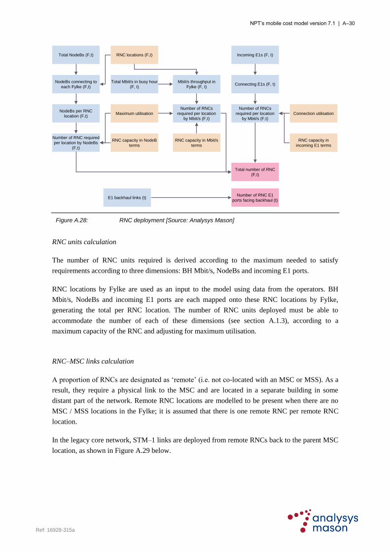
NPT’s mobile cost model version 7.1 | A–30
Ref: 16928-315a
RNC locations (F,t)
RNC capacity in NodeB
terms
Maximum utilisation
Total NodeBs (F,t)
NodeBs connecting to
each Fylke (F,t)
NodeBs per RNC
location (F,t)
Number of RNC required
per location by NodeBs
(F,t)
Total number of RNC
(F,t)
Total Mbit/s in busy hour
(F, t)
Mbit/s throughput in
Fylke (F, t)
Number of RNCs
required per location
by Mbit/s (F,t)
RNC capacity in Mbit/s
terms
Incoming E1s (F, t)
Connecting E1s (F, t)
Connection utilisation
Number of RNCs
required per location
by Mbit/s (F,t)
RNC capacity in
incoming E1 terms
E1 backhaul links (t)Number of RNC E1
ports facing backhaul (t)
Figure A.28: RNC deployment [Source: Analysys Mason]
RNC units calculation
The number of RNC units required is derived according to the maximum needed to satisfy
requirements according to three dimensions: BH Mbit/s, NodeBs and incoming E1 ports.
RNC locations by Fylke are used as an input to the model using data from the operators. BH
Mbit/s, NodeBs and incoming E1 ports are each mapped onto these RNC locations by Fylke,
generating the total per RNC location. The number of RNC units deployed must be able to
accommodate the number of each of these dimensions (see section A.1.3), according to a
maximum capacity of the RNC and adjusting for maximum utilisation.
RNC–MSC links calculation
A proportion of RNCs are designated as „remote‟ (i.e. not co-located with an MSC or MSS). As a
result, they require a physical link to the MSC and are located in a separate building in some
distant part of the network. Remote RNC locations are modelled to be present when there are no
MSC / MSS locations in the Fylke; it is assumed that there is one remote RNC per remote RNC
location.
In the legacy core network, STM–1 links are deployed from remote RNCs back to the parent MSC
location, as shown in Figure A.29 below.

NPT’s mobile cost model version 7.1 | A–31
Ref: 16928-315a
RNC locations (F,t)
MSC / MSS locations
(F,t)
RNC locations mapped
to MSC / MSS locations
(F,t)
Remote and co-located
RNC locations (F,t)
Total Mbit/s in busy
hour (F, t)
Total BH Mbit/s mapped
to Fylke (F,t)
BH Mbit/s per remote
RNC location (F, t)
STM-1 capacity and
utilisation
Number of STM-1 links
(F,t)
Distance of STM-1 links
(F,t)
Fylke-to-Fylke distance
matrix
Figure A.29: RNC–MSC
remote transmission in
the legacy core network
[Source: Analysys
Mason]
The BH Mbit/s transiting through these RNCs is backhauled to the MSC using STM–1 leased
lines. Remote RNCs require physical RNC–MSC links and the total number of these is calculated
from the total number of remote RNCs and the link capacity required.
The total traffic handled by each remote RNC can be calculated using the total BH Mbit/s. The
average traffic handled by each remote RNC is then converted into an equivalent number of STM–
1 links, adjusted for maximum utilisation.
The distance of these links is also an important output of the model as the backhaul costs involve a
connection charge per link end and a distance-based cost.
The distances between all of the Fylker are specified in the NtwDesBase worksheet according to
straight-line distances between the major conurbations in each Fylke, adjusted for route length
using a multiplier of 1.3 (accounting for the non-straight line nature of networks given topology
constraints). The calculation of the distances of the RNC–MSC links uses this Fylke distance
matrix, in combination with the mapping of RNCs locations onto MSCs locations, which is
performed in the RNCMSC worksheet.
Incoming and outgoing ports
The incoming ports to the RNC are ports facing the NodeB, whilst the outgoing ports in the legacy
core network are ports facing the MSC. Figure A.30 below shows the constituents of the incoming
and outgoing ports.
The total number of E1 incoming ports into RNC is the sum of microwave and leased line
backhaul links, whilst the total number of outgoing ports is calculated from the total number of
RNCs and total BH Mbit/s traffic, accounting for minimum deployment, utilisation and
redundancy.
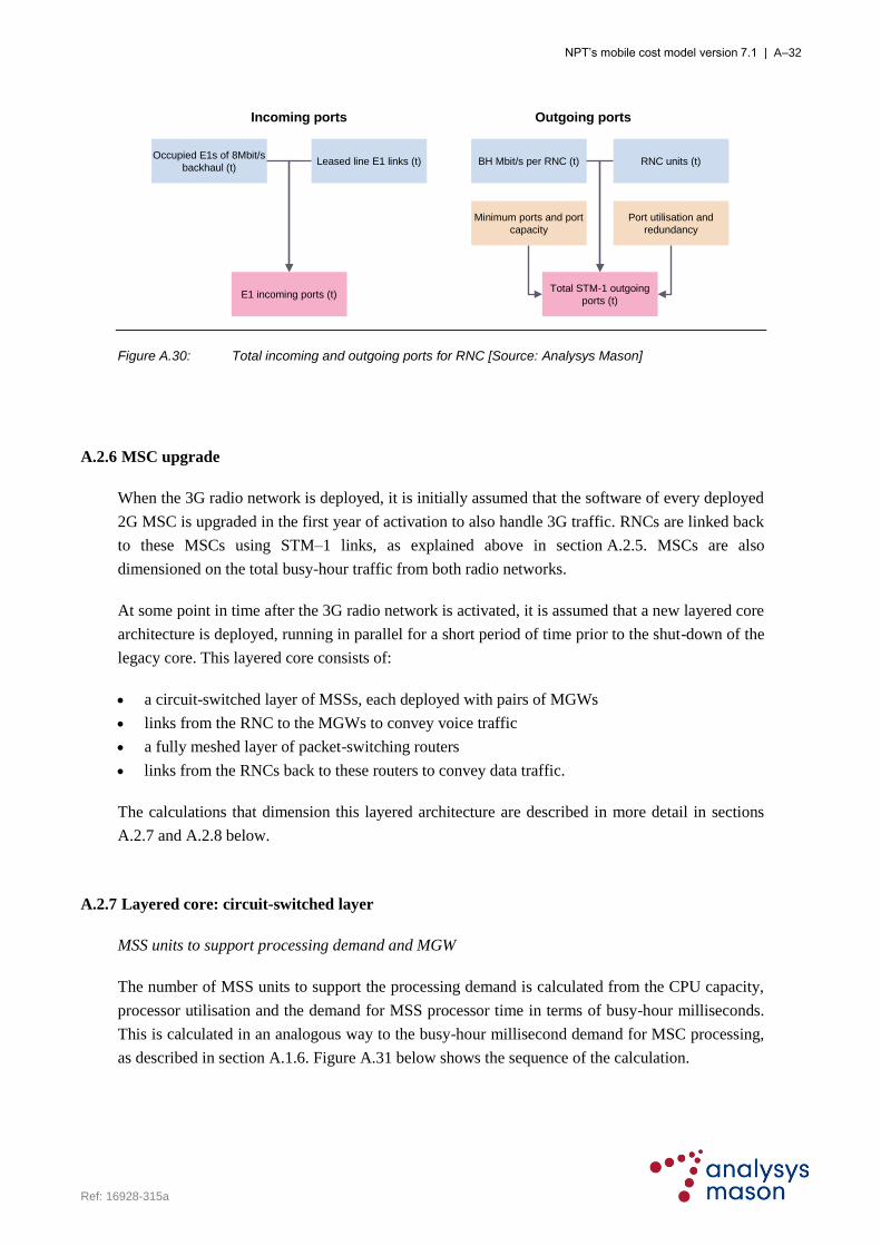
NPT’s mobile cost model version 7.1 | A–32
Ref: 16928-315a
E1 incoming ports (t)
BH Mbit/s per RNC (t)
Incoming ports Outgoing ports
Occupied E1s of 8Mbit/s
backhaul (t)Leased line E1 links (t) RNC units (t)
Total STM-1 outgoing
ports (t)
Port utilisation and
redundancy
Minimum ports and port
capacity
Figure A.30: Total incoming and outgoing ports for RNC [Source: Analysys Mason]
A.2.6 MSC upgrade
When the 3G radio network is deployed, it is initially assumed that the software of every deployed
2G MSC is upgraded in the first year of activation to also handle 3G traffic. RNCs are linked back
to these MSCs using STM–1 links, as explained above in section A.2.5. MSCs are also
dimensioned on the total busy-hour traffic from both radio networks.
At some point in time after the 3G radio network is activated, it is assumed that a new layered core
architecture is deployed, running in parallel for a short period of time prior to the shut-down of the
legacy core. This layered core consists of:
a circuit-switched layer of MSSs, each deployed with pairs of MGWs
links from the RNC to the MGWs to convey voice traffic
a fully meshed layer of packet-switching routers
links from the RNCs back to these routers to convey data traffic.
The calculations that dimension this layered architecture are described in more detail in sections
A.2.7 and A.2.8 below.
A.2.7 Layered core: circuit-switched layer
MSS units to support processing demand and MGW
The number of MSS units to support the processing demand is calculated from the CPU capacity,
processor utilisation and the demand for MSS processor time in terms of busy-hour milliseconds.
This is calculated in an analogous way to the busy-hour millisecond demand for MSC processing,
as described in section A.1.6. Figure A.31 below shows the sequence of the calculation.

NPT’s mobile cost model version 7.1 | A–33
Ref: 16928-315a
MSS CPU CapacityMSS processor
Utilisation
Total BHms demand for
MSS (t)
Required number of
processors for BHms
demand (t)
MSS processor
capacity
MSS units required to
support processor BHms
demand (t)
Minimum number of
MSS units ( t)MSS units required (t)
MSS locations (F, t)
MGW per MSS MGW units required (t)
Figure A.31: Calculation
of MSS units to support
processing demand and
MGW [Source: Analysys
Mason]
Taking into account the MSS processor utilisation, the total number of processors required to meet
the demand can be calculated as the total number of busy-hour milliseconds (BHms) divided by
the effective MSS capacity. We have assumed MSS locations by Fylke over time and have also
calculated the number needed to meet processing demand – the actual number of MSS deployed is
then the larger of the two. From this, the number of MSS within and outside of Oslo is then
calculated.
It is assumed that two MGWs are deployed per MSS, meaning that the number of MGWs deployed
follows directly, hence the number of MGWs within and outside Oslo can also be calculated.
Inter-MGW infrastructure
The inter-MGW port and link requirements are considered according to three separate cases:
between MGW sites within Oslo (if there are multiple MSS locations in Oslo): these are
assumed to lie on a single ring structure
between co-sited MGWs outside of Oslo
between MGWs outside of Oslo: these are assumed to sit on a resilient ring.
The calculation of MGW–MGW links between Oslo sites are shown in Figure A.32 below.

NPT’s mobile cost model version 7.1 | A–34
Ref: 16928-315a
RNCs mapped onto
MGW locations (F, t)
RNC-MGW BHE (F,t)
BHE by MGW (Fylke, t)
Proportion of BHE lying
in Oslo (t)
MGW and MSC BHE
(F,t)
Traffic distributions for
2G and 3G (F)
STM1 capacityIntra-Oslo ring capacity
(t)
Total BHms demand for
MSS (t)
Number of intra-Oslo
ring links (t)
Length of intra-Oslo ring
links (t)
Blocking probabilityInter-switch and
voicemail BHE (t)
Average length per intra-
Oslo link
Figure A.32: Calculation
of MGW–MGW links
between Oslo sites
[Source: Analysys
Mason]
It is assumed that all of these MGWs lie on a ring structure within Oslo. In order to calculate the
capacity required for this ring, the proportion of BHE that occur within Oslo is first determined.
To calculate this, the MGW and MSS BHE by Fylke is derived, using the traffic distributions for
2G and 3G. The BHE is then aggregated to the Fylker containing MGWs (the Fylker with MSSs),
based on the calculated mapping of RNC to MGW. This allows the calculation of the proportion of
BHE not associated with the MGWs in Oslo.
This proportion is applied to the BHE for inter-switch and voicemail traffic and the Erlang B table
is used to calculate the number of channel equivalents required on the ring. The number of STM–1
equivalents needed to accommodate these channels is then calculated, accounting for a maximum
utilisation percentage. The number of STM–1 links required is this number of STM–1 per ring-
link multiplied by the number of links in the ring (i.e. the number of MGWs in Oslo). An average
link length of 3km is assumed, to derive the total length of STM–1 links required.
The calculation of MGW–MGW links between non-Oslo sites is shown below in Figure A.33.

NPT’s mobile cost model version 7.1 | A–35
Ref: 16928-315a
Proportion of BHE lying
outside of Oslo (t)
STM1 capacityIntra-Oslo ring capacity
(t)
Number of intra-Oslo
ring links (t)
Length of intra-Oslo ring
links (t)
Blocking probabilityInter-switch and
voicemail BHE (t)
Average length per intra-
Oslo link
MSS locations outside of
Oslo (t)
MGW outside of Oslo (t)
Co-sited MGW-MGW
links (t)
(a) (b)
Figure A.33: Calculation of MGW–MGW links between (a) co-sited MGWs outside of Oslo and (b)
MGWs outside of Oslo [Source: Analysys Mason]
The links between co-sited MGWs outside of Oslo are assumed to be equal to half the number of
MGWs outside of Oslo (i.e. one link per pair).
The MGWs outside of Oslo are assumed to sit on a „resilient double ring‟ as detailed in section 4.2.
The capacity of each ring is calculated in the same manner as the Oslo ring, but using the BHE
occurring outside of Oslo. The number of STM–1 links on the ring is also derived in the same
way. An average link length on the ring is assumed, and this is multiplied by the number of links
to obtain the total length of STM–1 links.
MGW ports calculation (RNC-facing, interconnect-facing, VMS-facing)
Figure A.34 below shows how the number of RNC-facing ports is derived.
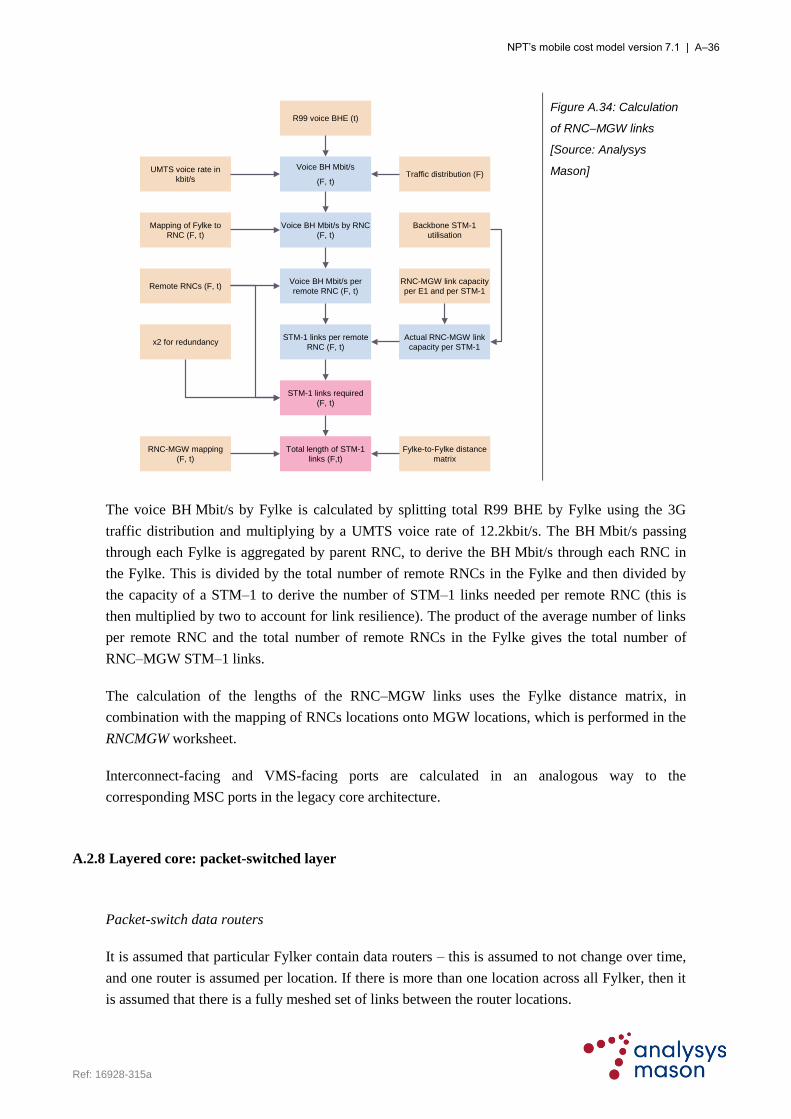
NPT’s mobile cost model version 7.1 | A–36
Ref: 16928-315a
R99 voice BHE (t)
Actual RNC-MGW link
capacity per STM-1
Voice BH Mbit/s
(F, t)
RNC-MGW link capacity
per E1 and per STM-1
Backbone STM-1
utilisation
x2 for redundancy
UMTS voice rate in
kbit/sTraffic distribution (F)
Mapping of Fylke to
RNC (F, t)
Voice BH Mbit/s by RNC
(F, t)
Voice BH Mbit/s per
remote RNC (F, t)Remote RNCs (F, t)
STM-1 links per remote
RNC (F, t)
STM-1 links required
(F, t)
Total length of STM-1
links (F,t)
RNC-MGW mapping
(F, t)
Fylke-to-Fylke distance
matrix
Figure A.34: Calculation
of RNC–MGW links
[Source: Analysys
Mason]
The voice BH Mbit/s by Fylke is calculated by splitting total R99 BHE by Fylke using the 3G
traffic distribution and multiplying by a UMTS voice rate of 12.2kbit/s. The BH Mbit/s passing
through each Fylke is aggregated by parent RNC, to derive the BH Mbit/s through each RNC in
the Fylke. This is divided by the total number of remote RNCs in the Fylke and then divided by
the capacity of a STM–1 to derive the number of STM–1 links needed per remote RNC (this is
then multiplied by two to account for link resilience). The product of the average number of links
per remote RNC and the total number of remote RNCs in the Fylke gives the total number of
RNC–MGW STM–1 links.
The calculation of the lengths of the RNC–MGW links uses the Fylke distance matrix, in
combination with the mapping of RNCs locations onto MGW locations, which is performed in the
RNCMGW worksheet.
Interconnect-facing and VMS-facing ports are calculated in an analogous way to the
corresponding MSC ports in the legacy core architecture.
A.2.8 Layered core: packet-switched layer
Packet-switch data routers
It is assumed that particular Fylker contain data routers – this is assumed to not change over time,
and one router is assumed per location. If there is more than one location across all Fylker, then it
is assumed that there is a fully meshed set of links between the router locations.
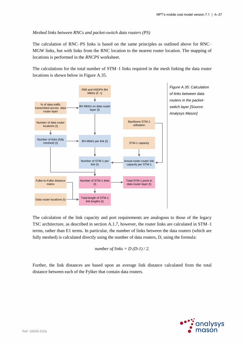
NPT’s mobile cost model version 7.1 | A–37
Ref: 16928-315a
Meshed links between RNCs and packet-switch data routers (PS)
The calculation of RNC–PS links is based on the same principles as outlined above for RNC–
MGW links, but with links from the RNC location to the nearest router location. The mapping of
locations is performed in the RNCPS worksheet.
The calculations for the total number of STM–1 links required in the mesh linking the data router
locations is shown below in Figure A.35.
R99 and HSDPA BH
Mbit/s (F, t)
BH Mbit/s on data router
layer (t)
Number of STM-1 per
link (t)
Number of STM-1 links
(t)
Total STM-1 ports in
data router layer (t)
BH Mbit/s per link (t)
Fylke-to-Fylke distance
matrix
% of data traffic
transmitted across data
router layer
Number of data router
locations (t)
Number of links (fully
meshed) (t)
Actual router-router link
capacity per STM-1
STM-1 capacity
Backbone STM-1
utilisation
Data router locations (t)Total length of STM-1
link lengths (t)
Figure A.35: Calculation
of links between data
routers in the packet-
switch layer [Source:
Analysys Mason]
The calculation of the link capacity and port requirements are analogous to those of the legacy
TSC architecture, as described in section A.1.7, however, the router links are calculated in STM–1
terms, rather than E1 terms. In particular, the number of links between the data routers (which are
fully meshed) is calculated directly using the number of data routers, D, using the formula:
number of links = D (D-1) / 2.
Further, the link distances are based upon an average link distance calculated from the total
distance between each of the Fylker that contain data routers.

NPT’s mobile cost model version 7.1 | B–1
Ref: 16928-315a
Annex B: Glossary
Acronym Meaning Acronym Meaning
2G Second generation of mobile telephony M-F Mobile to fixed
3G Third generation of mobile telephony M-M Mobile to mobile
AUC Authentication centre MMS Multimedia message service
BH Busy-hour MMSC MMS centre
BHE Busy-hour Erlangs MN Mobile Norway
BSC Base station controller MSC Mobile switching centre
BTS Base transmitter station or base station MSS MSC server
CCH Control channel MT Mobile termination
CE Channel element MTR Mobile termination rate
CK Channel kit MVNO Mobile virtual network operator
CPU Central processing unit NC Netcom
DCS Digital cellular system NDA Non-disclosure agreement
E1 2Mbit/s unit of capacity NMS Network management system
EC European Commission NN Network Norway
ED Economic depreciation NodeB Denotes UMTS equivalent of a BTS
EGSM Extended GSM NOK Norwegian krone
EIR Equipment identity register NPT Norwegian Post and
Telecommunication Authority
EPMU Equi-proportional mark-up NR National roaming
FAC Fully-allocated cost OLO Other licensed operator
F-M Fixed to mobile PCU Packet control unit
GGSN Gateway GPRS serving node PDP Packet data protocol
GPRS General packet radio system PoI Point of interconnect
GSM Global system for mobile
communications PS Packet switch
GSN GPRS serving node PV Present value
HCA Historical cost accounting QAM Quadrature amplitude modulation
HLR Home location register R99 Release-99
HSDPA High speed downlink packet access RNC Radio network controller
HSPA High speed packet access SDCCH Stand-alone dedicated control channel
HSUPA High speed uplink packet access SGSN Subscriber GPRS serving node
IN Intelligent network SMS Short message service
IP Internet Protocol SMSC SMS centre
LRAIC Long-run average incremental cost SP Service provider
LRIC Long-run incremental cost SSB Statistics Norway
LTE Long-term evolution STM Synchronous transport module
MEA Modern equivalent asset T2 Tele2
MGW Media gateway UMTS Universal mobile telecommunications
systems

NPT’s mobile cost model version 7.1 | B–2
Ref: 16928-315a
Acronym Meaning Acronym Meaning
TCH Traffic channel VLR Visitor location register
TDD Time division duplex VMS Voicemail system
TN Telenor WACC Weighted average cost of capital
TRX Transceiver unit
TSC Transit switching centre
Figure B.1: Acronyms used throughout the document [Source: Analysys Mason]

NPT’s mobile cost model version 7.1 | C–1
Ref: 16928-315a
Annex C: Operator submissions in developing v6 (public)
C.1 Telenor
Neither the NetCom nor the Telenor model will be “actual operator models” because NPT has
decided to model the market without national roaming. A share of the third operator retail market
share is in the model assumed to be carried by NetCom and Telenor, but this traffic is distributed
similarly to other traffic. This assumption is evidently not reflecting realities since national
roaming traffic only is carried in the remote parts of NetCom‟s and Telenor‟s networks (the areas
outside the actual coverage area of the third operator). Thus, the Telenor and NetCom models are
not actual operator models.
► Analysys Mason response
National roaming traffic – a declining share of the retail base of the third operator – is included in
the model as traffic carried by Telenor and NetCom. Telenor is correct that this traffic is assumed
to be distributed similarly to its own traffic (from 2009 onwards when the third-operator network
starts service). However, with general migration off the incumbents‟ GSM networks, spare
capacity will appear across the GSM layer and the impact of carrying national roaming traffic will
be lower than the additional traffic volumes would indicate, and could even be zero. Accepting
this, we consider that the issue is whether the modelled Telenor and NetCom are materially
different from the (actual) Telenor and NetCom if that different traffic distribution were taken into
account. In our view, the outcome of the model being materially different from that of Telenor‟s
real situation is not true, given the following:
There is no (material) national roaming traffic until 2008, and therefore all costing aspects of
the GSM network up to the end of 2007 are unaffected. This means that the GSM parts of the
cost base are only marginally influenced by the presence of national roaming volumes in the
later years.
The actual national roaming traffic carried by Telenor (and NetCom) in 2008 has been added
to the model (it was excluded in the draft v5.1 model because of the difference in third-
network launch dates: 2008 in reality, 2009 in the model). However this traffic in the model is
explicitly excluded from the radio network dimensioning in 2008 – it is modelled as a separate
service for 2008 only, which does not contribute radio BHE. This means that, consistent with
the approach to carrying national roaming traffic, the networks of Telenor and NetCom are not
required to deploy additional sites, BTS or TRX capacity in cities in response to national
roaming volumes, and national roaming volumes essentially remain in remote parts of the
network. With our network calibration checks carried out for the latest network data provided
for 2008, then this should ensure that the model is not incorrectly sensitive to the actual traffic
volume distribution.

NPT’s mobile cost model version 7.1 | C–2
Ref: 16928-315a
From 2009 onwards, national roaming traffic forms a declining traffic volume for the two
incumbents as part of an overall declining share of the market. This volume is carried in the
model on a GSM network, which has spare capacity (because GSM volumes are in steady
decline due to 2G/3G migration), and carried on a UMTS network, which also has spare
capacity (because it has been deployed to serve the expected future loading of UMTS services
from the operator‟s own subscriber base). The proportion of the average incumbent traffic due
to national roaming is shown in Figure C.1. It should be noted that when national roaming
traffic is at the highest proportion (i.e. in 2009), then the national roaming traffic is distributed
most similarly to the incumbent‟s own traffic (i.e. still within many cities and urban areas
because the third entrant roll-out has yet to reach out into further regions). When national
roaming traffic is at the smallest proportion of volumes, then national roaming is most
„remote‟.
0%
10%
20%
30%
40%
50%
60%
2008
2009
2010
2011
2012
2013
2014
2015
2016
2017
2018
2019
2020S
hare
of
tota
l netw
ork
tra
ffic
for
the a
vera
ge
inc
um
bent
National roaming traffic per incumbent
Own traffic per incumbent (average)
Figure C.1: National
roaming traffic for an
average incumbent
[Source: Analysys
Mason]
The majority of radio network equipments (sites, BTS, NodeBs) are fully retained in the
network (with capex, ongoing replacement and opex) even if demand volumes decline (as
would clearly be the case going from 2008 to 2009 when the third entrant starts service). This
means in particular that the majority of the 2G network deployed at the peak of 2G demand
(i.e. around 2007–2009) is retained until 2020, even though the distribution of declining traffic
is non-uniform compared to the traffic distribution pre-national roaming at the peak of traffic
load.
To indicate the materiality of this national roaming traffic distribution point, the model can be
run with no national roaming traffic, by setting the third-operator network share to be equal to
its retail market share (equivalent to costing the incumbents with only their own traffic). The
LRIC+++ of termination for Telenor in this case is higher by 2% from 2009 to 2010. As such,
we estimate the maximum possible sensitivity to the (complete loss of) national roaming
NPT’s mobile cost model version 7.1 | C–3
Ref: 16928-315a
volumes is 2%. Therefore, given the economies of scale from carrying national roaming traffic
in the network, we consider that the impact of smaller adjustments to the model as a result of
distributional changes to own versus national roaming traffic will be much less than 1% and
would not increase the LRIC+++ cost of serving traffic on the network.
Costs associated with data services
The model estimates a cash flow of costs, op-ex and cap-ex. These costs are attributed to various
services so that all relevant costs are covered (in NPV terms) over the modelling period. The
economic depreciation algorithm is designed in order to ensure cost recovery in this sense.
The model yields cost recovery profiles for data services that clearly are out of line with what we
observe in the Norwegian markets (as well as most other mobile markets). As an example, if we
look at costs recovered by services carried by the 3G network in the period 2010 – 2042, data (R99
+ high speed) accounts for 40% - 50% of cost recovery in NPV terms. If we look at 3G cost
recovery in the year 2009 the pattern is the same. According to the model data will account for ca.
50% of 3G revenues. This is in contrast to current revenue shares for operators where data
typically account for 5% - 10% of revenues.
In the model itself, the focus is on cost recovery by service. However, in the conceptual design
document it is explicitly stated that the allocated cost are to be interpreted as prices/ revenues per
unit:
In the modelled environment of a competitive market, the price that will be charged per unit
demand is a function of the lowest prevailing cost of supporting that unit of demand, thus the price
will change in accordance with the costs of the modern equivalent asset for providing the same
service function. The shape of the revenue line (or cost recovery profile) for each asset class is
thus a product of the demand supported (or output) of the asset and the profile of replacement cost
(or modern equivalent asset price trend) for that asset class.
The modelling assumptions are based on observed data usage and forecasts of data usage in the
coming years. Necessary network capacity to carry the data volumes is significant. The growth in
data usage is driven by the current and forecasted price level for data services in the end user
market. As indicated above, current data prices generate 5 – 10% of revenues (and not 40%). This
is evidently inconsistent. If data had been priced according to the model results, current data use
would have been prohibitively expensive, and demand would have been significantly below the
volumes we observe today. In Telenor‟s opinion, NPT has two possible ways to ensure that the
model become consistent:
Alternative 1: Use data volumes in the model consistent with the model results, i.e. make forecasts
of data usage based on the assumption that the retail price of using data services are 4 – 6 times
higher than the price we observe in the market today.
Alternative 2: Develop other algorithms for cost allocation so that the data cost recovery becomes
aligned with market realities.

NPT’s mobile cost model version 7.1 | C–4
Ref: 16928-315a
► Analysys Mason response
Firstly, it should be noted that the model covers network expenditures, and a share of business
overheads allocated to network services. The model does not include retail expenditures.
Therefore, any comparison of the model results to actual revenues must be made in the
understanding that the distribution of retail cost recovery may be different to that presented in the
network cost model. In developing the results of the cost model, we apply no requirement as to
how any retail costs may be recovered by retail services, nor do we suggest that all network
services should be priced in the retail market according to the model results. The purpose of the
model is to calculate the network cost for mobile termination minutes as the basis for NPT‟s
cost-based pricing of wholesale termination.
Telenor assert that “if data had been priced according to the model results, current data use would
have been prohibitively expensive, and demand would have been significantly below the volumes
we observe today”. Telenor suggest therefore that the model recovers more costs per megabyte
than Telenor achieves in practice. As quoted in Annex D, Telenor assert that “it is not the case that
the modelling results are marginally wrong”.
We detail our response in Annex D due to the use of confidential Telenor data.
In conclusion, we reject Telenor‟s suggestion that the calculated LRIC+++ cost of mobile
termination is incorrect as a result of the allocation of cost to data services, and maintain that our
allocation of network costs to data is reasonable for the purposes of setting the basis for wholesale
voice call termination charges.
Market share third operator
The model assumes a retail market share for the hypothetical third operator of ca 15% in 2009.
The (voice) market share for the third operator is converging towards 33% in 2040. This profile is
based on the projections of third operator growth in version 4 of the model, combined with current
market shares of Tele2 and Network Norway. Telenor considers the assumed evolution of retail
market shares as plausible.
In the model it is assumed a significant difference between the retail market share and the
wholesale market share for the third network operator. According to the conceptual design
document this difference is driven by three variables:
· Third operator 2G coverage
· Third operator 3G coverage
· 2G – 3G migration in the market.
NPT’s mobile cost model version 7.1 | C–5
Ref: 16928-315a
This is explicitly stated in page 14:
”We shall estimate the rate of transfer to the third entrant on the basis of its network population
coverage and the 2G-to-3G migration rate of subscribers in the market.”
This is in contrast to the information provided in Analysys Mason presentation August 18: where
it is indicated on slide 23 that the difference between retail and wholesale market shares are also
driven by two additional variables:
· Proportion of own traffic on 2G
· Proportion of own traffic on 3G
According to the presentation, these variables (only the 2G variable is explained) are included
because: There is limited capacity in the operator‟s 2G layer, therefore only a limited proportion of
usage can be carried by the third network compared to national roaming.
Telenor‟s interpretation of this statement is that NPT assumes capacity constraints in the third
operator network within the area where the third operator has coverage. This is not a plausible
assumption. Why should the third operator invest in a network that is capacity constrained from
day one? An economically rational network roll out would be to install sufficient capacity to carry
all “own” traffic where the network has coverage. Furthermore, in the LRIC model, the network of
the (hypothetical) third operator is dimensioned to carry the traffic that is being assumed. Thus the
postulated capacity constraints are neither founded in a rational network roll-out strategy, nor in
the hypothetical third operator network.
Finally, the implemented calculation of third operator market share in the spreadsheet is neither
consistent with the conceptual design nor the formula in the August 18 presentation of the
following reasons:
1. The formula includes a variable “Average 2G proportion” (line 63). It seems that this variable
corresponds to Proportion of own traffic on 2G from the August 18 presentation. The formula does
not deploy a variable corresponding to Proportion of own traffic on 3G, instead the 3G calculation
includes (1 – avg 2G prop). There is no reason to believe that the available capacity in 2G and 3G,
relative to retail market shares and network coverage, move exactly similarly, but in opposite
directions. Furthermore, the assumed average 2G proportion in the spreadsheet decrease steadily
over time indicating that the 2G network of the third operator becomes increasingly more capacity
constrained (e.g. 70% in 2010 and 30 % in 2016). This is implausible.
2. The coverage assumptions in the formula for calculating market shares differ from the assumed
population coverage in the same model. There is a systematic downward bias. According to sheet
A5_NtwDesSlct, 2G population coverage is 52%, whereas 50% is assumed in the market share
formula. Furthermore there seems to be a 1 year offset in the 3G market shares. According to sheet
A5, the third operator obtains 3G population coverage of 81% in 2010 and 90% in 2011, whereas
the market share calculations assumes 70% in 2010 and 80% in 2011.

NPT’s mobile cost model version 7.1 | C–6
Ref: 16928-315a
Furthermore, the percentage of the third operator‟s traffic that is on-net will be greater than its
percentage of population coverage as in general usage tends to be more concentrated than
population and in particular the customer acquisition efforts of the third operator are more
focussed on the urban areas in which they have more on-net traffic than in uncovered areas.
Telenor urges NPT to implement market share calculations consistent with the conceptual design
document. Thus (only) the following variables are taken into account when calculating third
operator network market share:
· Third operator 2G coverage
· Third operator 3G coverage
· 2G – 3G migration in the market.
If NPT is of the opinion that such calculations results in too rapid growth in the wholesale market
share for the third operator, compared to their expectations, then it is a indication that the assumed
network roll out (coverage) for the third operator is too optimistic relative to NPT expectations.
At the meeting on 22 September, NPT/Analysys confirmed that the obvious way to calculate the
wholesale market share of the third operator is to let it be a function of 2G coverage area, 3G
coverage area and 2G – 3G migration (i.e. share of 2G and 3G customers). Thus, the wholesale
market share of the third operator should be calculated by the following formula:
Wholesale share = retail share * [2G share * 2G coverage + 3G share * 3G coverage]
Aspects of Telenor‟s roaming agreement with Network Norway were also discussed.
► Analysys Mason response
Analysys Mason has revised the calculation of the network market share profile of the third
operator; the retail market share profile of the third operator has not been altered. Also, the
population coverage of the third operator is calculated separately on the 3rdOpCov worksheet, so
that it automatically applies to the network market share calculation.
The market share is now calculated based on the formula:
Retail market share [(Proportion of handsets that are 2G) (2G coverage)] +
[(Proportion of handsets that are 3G) (total coverage)]
The „total coverage’ term is used in the formula for 3G handsets because 3G handsets can access
both 2G and 3G coverage (where complementary).
This revised network share (v6) is higher than that applied in the draft model (v5.1) – we conclude
it is broadly valid to accept that if the third operator covers x% of the Norwegian population with

NPT’s mobile cost model version 7.1 | C–7
Ref: 16928-315a
its network, then it should carry at least x% of the traffic offered by its subscriber base. These
market shares are shown below in Figure C.2.
-%
5%
10%
15%
20%
25%
30%
35%
2008
2010
2012
2014
2016
2018
2020
2022
2024
2026
2028
2030
2032
Mark
et
share
, yea
r end
Retail market share Third entrant v6 Third entrant v5.1
Figure C.2: Comparison
of market shares for third
operators [Source:
Analysys Mason]
As a result of this adjustment, the third operator‟s network may become traffic-driven early on in
its evolution, and may be required to deploy additional capacity within its coverage area.
Investments by third operator financed by current MTR margin
Network Norway and Tele2 are in the current regulatory period allowed to have a termination rate
significantly above the symmetric rate of Telenor and NetCom. The rationale for this asymmetry is
that it is supposed to generate revenues sufficient to cover the investment costs of building a third
network with 75 % population coverage. This is explicitly stated in the Ministry‟s decision. As an
example, consider the Network Norway appeal decision, page 21:
Based on a holistic evaluation of the situation and a weighting of interests with regard to the
circumstances discussed in the chapter above, the Ministry finds it appropriate to establish as a
governing objective that the higher revenue for the new network builders should basically be
equivalent to the investment costs of building a third mobile network. The Ministry assumes a
mobile network that is intended to cover 75 per cent of the population by the end of 2011 as is set
out in Mobile Norway’s business plan and which the companies have referred to in their appeals.
The Ministry considers it appropriate to permit Tele2 and Network Norway a milder form of
regulation up until the accumulated higher revenue matches the investment costs.
It is important to have in mind that Network Norway and Tele2 extract the higher termination
revenues on a significantly larger volume than what is reflected in the third operator LRIC model
since they have a considerable volume through MVNO agreements.

NPT’s mobile cost model version 7.1 | C–8
Ref: 16928-315a
It follows from the Ministry‟s decision that the capex of a network with 75% population coverage
is covered by the current termination margins. Thus, NetCom, Telenor Mobil and the fixed
operators are currently financing the network rollout for a third operator with 75% population
coverage. Then it is inconsistent to include this cost in the cash flow of the third operator. It is
even possible to argue that the cost associated with 75% population coverage should be included
in NetCom‟s and Telenor‟s cost cash flows.
Telenor is of the view that the capex associated with 75% population coverage should be
disregarded in the cost cash flow of the third operator in the LRIC modelling. This can be
implemented e.g. by hard coding capex unit costs to zero in the relevant period. Otherwise,
players in the Norwegian market will contribute to the network roll out of the third operator twice.
First by the full financing scheme due to the Ministry and then via cost allocation rules in the
LRIC model where a certain part of investment costs are allocated to call termination.
► Analysys Mason response
The model is capable of calculating costs on a number of different bases (e.g. LRIC+, pure LRIC)
as necessary for NPT‟s price-setting activities. The model has been extended so that variants of
cost can also be calculated, as described by Telenor above. In summary, the model can now
calculate the costs of the third operator in the situation where some roll-out costs are recovered
elsewhere (e.g. by asymmetric termination).
We do not comment on the relevance of these results for price setting. Further details of the model
modifications are provided in Annex F.2.
Economic depreciation
Telenor notes that NPT intends to retain the previous model‟s economic depreciation calculation
to recover incurred network expenditures over time. In 2006 Telenor pointed out and documented
that the economic depreciation calculation used in that model had comprehensive weaknesses and
flaws. Nevertheless, NPT adopted this economic depreciation calculation disregarding Telenor‟s
comments.
Telenor emphasises that the same weaknesses and flaws that were pointed out by Telenor in 2006
apply just as much to this new model. The formula for allocating costs over time proposed by NPT
has some properties that are very “uneconomical”, in particular the emphasis on historic events.
Events in the past have an effect on the allocation of costs into the infinite future. For a more
complementary description of the weaknesses and flaws of the economic depreciation formula, we
refer to Telenor‟s written responses in 2006 and the R&D Research Note 11/2006 “A note on
Economic depreciation” by Bjørn Hansen and Helene Lie Røhr.
Telenor notes that in the new model the economic depreciation calculation is used for both LRIC
and pure LRIC. Telenor is somewhat taken aback by the lack of attention and reflection regarding
the appropriateness of this economic depreciation used on calculation of pure LRIC. The
weaknesses and flaws pointed out by Telenor apply even stronger for calculation of avoidable
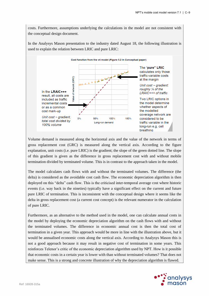
NPT’s mobile cost model version 7.1 | C–9
Ref: 16928-315a
costs. Furthermore, assumptions underlying the calculations in the model are not consistent with
the conceptual design document.
In the Analysys Mason presentation to the industry dated August 18, the following illustration is
used to explain the relation between LRIC and pure LRIC:
Volume demand is measured along the horizontal axis and the value of the network in terms of
gross replacement cost (GRC) is measured along the vertical axis. According to the figure
explanation, unit costs (i.e. pure LRIC) is the gradient; the slope of the green dotted line. The slope
of this gradient is given as the difference in gross replacement cost with and without mobile
termination divided by terminated volume. This is in contrast to the approach taken in the model.
The model calculates cash flows with and without the terminated volumes. The difference (the
delta) is considered as the avoidable cost cash flow. The economic depreciation algorithm is then
deployed on this “delta” cash flow. This is the criticised inter-temporal average cost where historic
events (i.e. way back in the nineties) typically have a significant effect on the current and future
pure LRIC of termination. This is inconsistent with the conceptual design where it seems like the
delta in gross replacement cost (a current cost concept) is the relevant numerator in the calculation
of pure LRIC.
Furthermore, as an alternative to the method used in the model, one can calculate annual costs in
the model by deploying the economic depreciation algorithm on the cash flows with and without
the terminated volumes. The difference in economic annual cost is then the total cost of
termination in a given year. This approach would be more in line with the illustration above, but it
would be annualised economic costs along the vertical axis. According to Analysys Mason this is
not a good approach because it may result in negative cost of termination in some years. This
reinforces Telenor‟s critic of the economic depreciation algorithm used by NPT. How is it possible
that economic costs in a certain year is lower with than without terminated volumes? That does not
make sense. This is a strong and concrete illustration of why the depreciation algorithm is flawed.

NPT’s mobile cost model version 7.1 | C–10
Ref: 16928-315a
NPT does not take account of the cost approaches in the model with LRIC and pure LRIC
calculated on different bases. A reasonable alternative approach should be to use pure-LRIC as the
basis for calculating LRIC, with the application of mark-ups to the pure-LRIC costs. NPT should
establish LRIC costs based upon a mark-up to pure LRIC and consider this as a reasonable
alternative.
► Analysys Mason response
We do not repeat our conclusions on the economic depreciation calculation from the previous
process in 2006 and 2007. Figure 5.2 from the Conceptual Design Document was adapted for the
extract returned by Telenor to illustrate the calculation of pure LRIC. The cost function refers to
network GRC; however, as Telenor explains, the model does not calculate pure LRIC using GRC.
Instead it uses (the difference in) the present value of network expenditures. As such, this diagram
incorrectly states the cost function axis in GRC terms, which should read “Illustrative PV of
network expenditures.”
Analysys Mason rejects Telenor‟s assertion on the lack of attention in this area: time has been
spent understanding the interaction between economic depreciation and pure incremental costs in
our mobile cost models, including NPT‟s v5.1. Only in simple or certain types of models (e.g.
single year, static depreciation calculation) will the pure LRIC calculation of avoidable costs
function in a uniform way. In models that are developed to be more complex (e.g. reflecting the
actual time-evolution of operators, using non-uniform demand profiles) then calculating the
avoidable cost of one particular service will require investigation.
As a result of our work in this area, we have concluded that whilst the full-time-series economic
depreciation method fits well with the calculation of LRIC+++ costs over the lifetime of the
modelled mobile businesses, it is less suited to calculating avoidable costs in some situations. In
particular, this unsuitability arises when the avoidable increment of demand is not a uniform
proportion of demand over time (as is the case with wholesale mobile termination supplied over
Telenor‟s and NetCom‟s networks). As Telenor has submitted, this results in (undesirable)
increased inter-temporal effects, which means that while costs may be (overall) lower without
wholesale termination, cost recovery is also moved forwards/backwards in time according to the
profile of residual demand applying to each network element. With data services more important
in the later years, this can mean that costs without wholesale termination are postponed more into
the future relative to the all-service calculation. As such, unconstrained pure incremental costs can
be very low or negative in later years.
Therefore we believe that an alternative calculation of pure LRIC is required. We adopted an
alternative approach in the draft v5.1 cost model issued to industry parties. In this situation, the
pure LRIC is calculated from the (present value) difference in network expenditures arising from
the removal of the wholesale termination volume, constrained over time so that the underlying
equipment price trends apply also to the pure LRIC components of cost (just as these price trends
apply to the LRIC+++ components of cost). We consider it reasonable that the calculated pure
LRIC is directly constrained by the equipment price trends for the same reason that the LRIC+++

NPT’s mobile cost model version 7.1 | C–11
Ref: 16928-315a
should reflect the (declining) underlying costs of supporting traffic volumes with network
equipment.
It is plausible (counter to Telenor‟s suggestion above) that the removal of mobile termination
volumes causes certain costs to be higher than otherwise: as an example, we could consider radio
sites and ancillary costs, which have an increasing site cost trend (as in the revised v6 model).
Removing termination volumes may result in some sites being deployed later in time – with rising
site costs, it could indeed appear (in particular years) that costs were higher without termination.
However, over the lifetime of the network, as in our pure LRIC calculation, this effect does not
dominate the overall cost calculation and the pure LRIC is calculated to be a small (positive) value
per minute when compared to the LRIC+++.
As a cross-check to our calculated pure LRIC for Telenor, we have estimated a pure incremental
cost result by:
starting with Telenor‟s LRIC+++ of mobile termination per minute
removing the +++ mark-ups for overheads, location updates and network common costs
removing the contribution to the remaining LRIC of network elements that are assumed to be
insensitive to traffic volumes (e.g. core switches and inter-switch transmission)
comparing the resulting sub-components of LRIC with the pure LRIC calculated by our
method.
This comparison (chart provided in Annex D) shows two important conclusions:
the level of cost per minute calculated by our pure LRIC method is similar to that obtained
by starting from the (accepted) LRIC+++ result and removing common and traffic-insensitive
cost components
the trend over time in the pure LRIC cost is similar to that obtained by starting from the
LRIC+++.
Consequently, we believe that our primary method of calculating the pure LRIC is reasonable and
justified, and a suitable basis on which NPT could consider setting pure-LRIC-based rate
regulation.
Third operator LRIC relative to roaming cost
The third operator has two basis ways of producing mobile services, either it can build a mobile
network and produce the traffic itself, or it can buy traffic within a national roaming agreement.
The third operator will choose between these two options, and combine these options in a way that
economize the corporate profitability.

NPT’s mobile cost model version 7.1 | C–12
Ref: 16928-315a
This principle will lead to the fact that the third operator will seek to build own network in areas
where the traffic volume is sufficient to bring the unit cost below their alternative cost. The
alternative cost is given by the prices in the national roaming agreement. The prices today in the
national roaming agreement between Telenor and Network Norway are far below the HCA cost by
services in 2009 and the years ahead. This seems strange all the time the third operator is expected
to economize the corporate profitability. Telenor encourage NPT to investigate these
circumstances and ensure that assumptions in the new LRIC model are in accordance with
operators expected actions in the market.
► Analysys Mason response
We agree with Telenor‟s view that it is important to compare the costs calculated for the third
network with the corresponding prices that might be available through national roaming
agreements.
However, it is necessary to compare these costs across all services (voice, SMS and data), since we
expect that there may be incentives for host operators to agree higher/lower prices for particular
services, and as Telenor explain under the heading of “data services,” it is evident that some retail
services provide more margin over the network cost than other services. Thus it is relevant to
compare the third operator results across all of the services carried. As an example, voice prices
may appear closely comparable (indicating a relative balance for build or buy decisions within a
third entrant‟s business) whereas SMS service prices may be unprofitable for a nationwide
provider relying on national roaming for SMS.
A chart comparing the third operator‟s costs and Telenor‟s national roaming prices is provided in
Annex D.
Costs related to frequencies
It seems that 3G licence fee payments not are taken into account in the new LRIC model. Telenor
invested 200 million NOK for the 3G licence in 2000, and we assume that renewals of the licence
will include new payments by Telenor in the future. As far as we understand the new LRIC model
these costs are not included in the model.
The LRIC calculation assumes that all traffic migrates to 3G by 2020, i.e. the 2G network are
being closed from the same point in time, and that payment of 2G annual licence fees ceases in
2020. But coverage by UMTS 900 is assumed from 2011 as traffic is migrated off 2G and
spectrum is re-farmed. This means that the 900 frequencies are utilized after 2020, and that both
annual licence fees and renewal costs for the frequencies should be included in the new model.
► Analysys Mason response
Regarding the issue of 3G licence fee payments, a new asset called “3G licence fee payments” has
been included in the model. This asset has an associated capex of NOK200 million, first paid in
2002 and every 12 years thereafter. In real terms, licence fees are assumed to be constant.

NPT’s mobile cost model version 7.1 | C–13
Ref: 16928-315a
Regarding the issue of 2G licence fees, the “2G licence fee payments” and “2G annual licence
fees” assets have had their fees split up to reflect costs related to GSM and to UMTS 900:
Fees (both one-off and annual) estimated to correspond to a 25MHz carrier have been
transferred from the 2G licence assets to the 3G licence equivalents in the relevant year. These
costs are then recovered over the lifetime of the 3G network
Fees for the remaining GSM spectrum are only charged for and recovered during the lifetime
of the GSM network.
The “3G licence fee payments,” “3G annual licence fees” and “2G annual licence fees” assets
previously had „asset smoothing‟ applied on the FullNw worksheet. This led to an underestimation
of the licence fees over time. Asset smoothing has been switched off for these three assets, and
therefore periodic licence fees are re-incurred in full every 12 years.
Capacity costs
The model provides for additional capacity first by increasing TRX‟s, sectorisation and then by
adding new sites. However, each of these is at a uniform cost (i.e. so each new site costs the same
as the previous new site). However, the real effect of traffic concentration is to require new
capacity and sites in areas where it is increasingly difficult to find appropriate sites and for which
the costs increase significantly. The impact of these real-world constraints are that the additional
cost of new sites is increasing, and the effective capacity provided by those sites is falling. Telenor
expects that this will be taken into account in the new model.
► Analysys Mason response
In response to both this comment and the one below, we have included a real-terms positive cost
trend for the radio assets in the model. This will reflect the fact that capacity-driven sites acquired
in later years have a higher real-terms cost than those in earlier years.
Whilst we have implemented an increasing site cost trend, we have not reflected the suggestion
that “the effective capacity provided by those sites is falling”. While site availability may be
reducing, we believe there is no strong reason to assume that sites installed for capacity have
materially reducing capacity. For example, radio equipments such as BTS and TRX (900 and
1800, dual band equipment and antennas, etc.) are becoming smaller and antenna technology is
improving all the time (particularly for environmentally-sensitive areas and shared sites), and so
there should not be significant capacity constraints to later sites caused by the limitations to site
availability.
Asset price trends
All the asset price trends used in the model are either flat or negative. In Telenor‟s view is this not
a good reflection of reality, as civil works makes up a significant part of network assets, and we

NPT’s mobile cost model version 7.1 | C–14
Ref: 16928-315a
would expect these to have a positive price trend. Telenor anticipates that NPT will change the
inputs in the model and introduce non-flat asset trends for labour-intensive assets.
Telenor has not sufficient detailed information in the accounting systems to illustrate that there
are increasing costs of finding new capacity sites. Regardless of information, this is however a
valid point. Capacity sites have to be located at ever more specific geographic locations in order
to function optimally in combination with the existing network topology. This leads to both cost
and capability effects; owners of potential capacity site locations are in a very strong bargaining
position towards mobile operators and can demand higher rentals and compromises in site design
and location limit the extent to which these sites can deliver their theoretical capacity.
According to Norwegian Statistics there has been a positive trend on labour cost related to road
construction: http://www.ssb.no/english/subjects/08/02/30/bkianl_en/tab-2009-08-21-01-en.html.
This information supports Telenor‟s view that labour-intensive assets in the model should have a
positive price trend.
► Analysys Mason response
In addition to the data from Statistics Norway on the construction cost index for road constructions
indicated above, we have also identified another set of indices on the construction costs for works
in offices and commercial buildings8 between 2000 and the present. In particular, the latter
provides an indication of the increase in costs for administrative expenses, labour costs and
materials relevant to civil, ancillary and utility works. The compound annual growth rate (CAGR)
of these indices, in real terms, are summarised below in Figure C.3:
Source Index CAGR Figure C.3: CAGR in real
terms between 2000 and
2009 by index [Source:
Analysys Mason
calculated from Statistics
Norway]
Road constructions Total costs 2.8%
Works in
commercial
buildings
Total costs 3.4%
Administrative expenses 1.8%
Labour costs 2.2%
Materials 4.3%
Based on these trends, we have therefore amended the capex and opex cost trends in the model as
follows:
Site acquisition and civil works now have a capex trend of +2% (based on the trend for labour
and administrative costs)
Radio ancillary equipment now have a capex trend of +4% (based on the cost trend of
materials)
Radio sites now have an opex trend of +2% (based on the cost trend of labour)
Switching sites also have a capex and an opex trend of +2%.
8 http://www.ssb.no/bkiror_en/
NPT’s mobile cost model version 7.1 | C–15
Ref: 16928-315a
Business overheads have not been adjusted on the basis that the mobile operators have significant
incentives to maintain their own level of efficiencies in this part of their business.
These trends are set in place for the period 2000–2013 in the model.
Costs related to decommissioning of 2G
Telenor is not convinced that costs related to decommissioning of 2G are taken into account in an
adequate way in the LRIC calculations, and invite NPT to explain this relation.
► Analysys Mason response
This issue was discussed in the previous modelling project: Telenor has not advanced further
information in addition to restating its opinion. Telenor has, however, supplied some
decommissioning costs for radio sites (see Annex D), which indicate that the cost to decommission
a site is a minor proportion of the modelled cost to acquire the site in the first place.
Consequently, we still believe the model contains sufficient costs to account for any
decommissioning costs faced by Telenor. As before, the purchasing algorithms of the model
continue to invest in the periodic replacement and operating expenditures of expiring network
elements in all years of the modelled GSM network, including in the later years when the network
is planned to be decommissioned (the model invests over NOK1billion during 2018, 2019 and
2020 in dedicated GSM equipment, all of which will be removed from the network by the
middle/end of 2020). This continued replacement expenditure for new assets is unlikely to occur in
a real network facing decommissioning, and therefore is retained in the model to reflect any
decommissioning costs.
MVNO
Telenor is surprised at the high level of LRIC and pure LRIC calculated for the generic MVNO.
Telenor invites NPT to explain these calculations more explicitly.
► Analysys Mason response
The „generic MVNO‟ has a market profile set up to acquire 5% of the market in all years and was
shared with all parties, but primarily for Telenor and NetCom to transparently observe the MVNO
calculations. It is not the MVNO equivalent of the third-operator calculation and is for illustrative
purposes only. The pure LRIC calculation for the MVNO results in a very low cost (close to zero)
because the model assumes a single mobile switch that is not modelled to be sensitive to MVNO
traffic volumes. We have not examined in detail whether the MVNO switch infrastructure is a
fixed cost (as the model assumes) or more variable in the long run (which would mean a higher
MVNO pure LRIC would be calculated, closer to the LRIC).
NPT’s mobile cost model version 7.1 | C–16
Ref: 16928-315a
C.2 NetCom
SCENARIO ANALYSES
We refer to the invitation, third paragraph, saying that NPT will carry out scenario analyses in
which the third network operator to a different extent establishes a separate network in parts of the
country and makes use of national roaming in mobile networks to obtain coverage beyond their
own network. It also appears that NPT has made computations showing that the costs with resting
on national roaming will not be significantly higher than the costs of version 5.1 for the third
network operator.
► Analysys Mason response
Computations involving national roaming prices have not been issued to industry parties for
consultation due to the confidential nature of national roaming agreements. The cost calculations
for the third network operator indicate that two results for voice traffic are broadly comparable:
the costs of the third operator with full national coverage
the costs of the third operator with sub-national coverage blended with current national
roaming prices.
This indicates that the modelled third operator is not operating outside of reasonable economic
boundaries with respect to voice costs/prices. The comparison for SMS and data services suggests
the same conclusion. The basis for setting wholesale termination rates will be the definitive results
from the issued cost model; scenarios and other tests carried out by NPT and Analysys Mason
serve to validate the reasonableness of the calculation, but do not form a basis for setting prices.
As such, it is considered unnecessary and distracting to submit various permutations, scenarios and
options for industry comment.
C.3 TDC
Market share
The model has provided for a market share of the generic MVNO at 5% of the Norwegian mobile
market. Market share is one of the major parameters for defining the cost for a mobile company.
TDC would like to underline that we are and will stay only at the business market. It is not a part
of our strategy to move over to the consumer market. Hence our number of subscribers will be
lower than a full scale MVNO. We have attached a updated outline of our marked share.
► Analysys Mason response
This market share has been implemented in the TDC model on the M6 worksheet.
NPT’s mobile cost model version 7.1 | C–17
Ref: 16928-315a
MVNO cost
Analysys Mason has set up a list for us showing the cost elements included in the model. In
addition to the elements on this list the following elements should be added: MSC, MSC ports,
Backbone links, Business overhead mark up.
► Analysys Mason response
The generic MVNO calculation is modelled with an MSS and MGW pair rather than the MSC
architecture, i.e. only one of these configurations is required in the long term. With regard to
backbone links, MVNOs do not need these links in their architecture for the purposes of MVNO
network activities, given their small, centralised network switch. As all telecoms providers
interconnect in Oslo, and all mobile networks have main switches in Oslo, there is no requirement
for MVNO-host traffic exchange to require a national backbone transmission network. We have
re-reconciled the MVNO costs to include relevant business overhead assets.
Depreciation lifetime
On the basis of the actual economic lifetime of the equipment in our network the time of
depreciation must be shorter. In Denmark the depreciation time is shorter than what our model
now shows, and we request that the model is updated with depreciation values more like HCA.
► Analysys Mason response
Figure C.7 below summarises the asset lifetimes provided in the public versions of the LRIC
models built by Analysys Mason for PTS9 in Sweden and NITA10 in Denmark, as well those in the
v6 mobile LRIC model for NPT in Norway.
9 http://www.pts.se/upload/Ovrigt/Tele/Bransch/Kalkylarbete%20mobilnät/Final-PTS-model-public-version-020608.zip
10 http://en.itst.dk/interconnection-and-consumer-protection/lraic/filarkiv-lraic/lraic-pa-mobil/horing-4-september-
2007/Modeludkast%20v.1.1.zip

NPT’s mobile cost model version 7.1 | C–18
Ref: 16928-315a
Norway years Denmark years Sweden years
Own tower acquisition,
civils 15 Owned macro site 25
Site acquisition,
preparation and lease 25
Third-party civils, site
ancillary 10 Third-party site 20
2G/3G cells,
TRX/channel kit, DXX,
HSDPA upgrades
8 GSM BTS, TRX, NodeB,
carriers, channel kit 10
2G/3G cells, TRX/channel
kit 10
Other backhaul links 8 Backhaul links, access
point 10 Backhaul links/upgrades 10
BSC/RNC base unit,
ports 8
BSC/RNC base unit,
ports 10
BSC/RNC base unit,
ports 10
2G MSC, 3G MSS, 3G
MGW, TSCs, ports 8
2G MSC, 3G MSS, 3G
MGW, associated ports 10
2G MSC, 3G MSS/MGW,
ports 10
BSC/MSC sites 20 MSC/remote BSC sites 25 MSC sites 25
MSC/MSS software 3 MSC/MSS/NMS software 5 2G. 3G MSC software 5, 7
VMS, HLR, AUC, EIR,
SMSC, billing system 6
IN, VMS, HLR, AUC,
EIR, SMSC, MMSC,
MNP
8
VMS, HLR equipment,
SMSC, IP transmission,
network management
centre
10
TSCs 20 Transit switches 10 Tandem/transit 10
PCU, GGSN, SGSN,
packet data routers 8
GPRS/EDGE-PCU,
GGSN, SGSN 10 PCU, GGSN, SGSN 10
IN, network management
system
annual
capex
Billing system, network
management system
hardware, content
platform
8
Interconnect interface,
switching support plant,
switch building
preparation
10
HLR software 6 HLR software 2
Figure C.4: Asset lifetimes (years) in public Scandinavian LRIC models [Source: Regulator websites]
The most material factors for the cost of voice termination are in the lifetimes for the radio sites,
which are 5–10 years shorter in the current Norwegian model, and in the lifetimes for major
mobile network BTS, NodeB, BSC, RNC and MSC equipment (around 8 years in the Norwegian
model compared to around 10 years in the other two models).
These comparisons indicate that the depreciation period for assets in the NPT model are
conservative when compared with the other Scandinavian jurisdictions, and there is no indication
that additional reduction in lifetimes would be appropriate.
Based on a consideration of a range of factors (including two topics related to site replacement
discussed confidentially with Telenor), NPT also considers it appropriate and broadly conservative
to maintain its existing site lifetimes of 15 years for owned sites and 10 years for third-party sites.

NPT’s mobile cost model version 7.1 | C–19
Ref: 16928-315a
C.4 Ventelo
Mobile broadband:
Telenor has 233.000 mobile broadband subscribers and a market share of 59% according to Q2
2009 financial reports. This implies a total market size of 392.000 mobile broadband subscribers.
The forecast in the model is too low as it shows 400.000 subscribers by year end 2009. We
estimate the volume for 2009 year end to state 500.000 subscribers. We also believe the saturation
level of the market will exceed 1.500.000 subscribers.
► Analysys Mason response
The NPT market data for mid-year 2009 is 380 000 subscribers, an increase of almost 120 000
subscribers since the end of 2008. Therefore, a year-end 2009 subscriber base of 500 000 appears
reasonable and we have revised our forecast accordingly. We have compared our penetration
forecast with that developed by Analysys Research11 and it appears to be broadly consistent, as
illustrated below in Figure C.5. Therefore, we have kept the modelled saturation level for mobile
broadband at 20% of the population.
0%
5%
10%
15%
20%
25%
30%
2007 2008 2009 2010 2011 2012
Penetr
ation
Model Analysys Research forecast
Figure C.5: Mobile
broadband penetration of
population in Norway
[Source: Analysys
Research]
In addition, we assume that the average usage for mobile broadband is too conservative in the
model. Our conclusion; either the base for pricing of voice is too high or the base for pricing
mobile broadband too low.
11 Mobile broadband in Europe: forecasts and analysis 2009–2014, May 2009

NPT’s mobile cost model version 7.1 | C–20
Ref: 16928-315a
► Analysys Mason response
We have updated the mobile broadband traffic per user values using NPT‟s mid-year 2009 market
information. In our view, this update indicates that our projection of 2000 HSDPA megabytes (and
500 HSUPA megabytes) per user per month may slightly overstate broadband volumes in the near
future. The forecasts in the two models are illustrated below in Figure C.6, with the forecast now
increasing to only 1600MB per subscriber per month (plus 400 HSUPA megabytes).
-
200
400
600
800
1,000
1,200
1,400
1,600
1,800
2,000
20
06
20
07
20
08
20
09
20
10
20
11
20
12
20
13
20
14
20
15
20
16
20
17
Ave
rag
e u
sa
ge
pe
r su
bscri
be
r p
er
mo
nth
(m
eg
ab
yte
s)
v5.1 forecast v6 forecast
Figure C.6: Market
average high-speed data
usage per subscriber per
month forecast in the
version 5.1 and version 6
models, excluding
Nordisk/ICE [Source:
Analysys Mason]
The NPT market data indicates that average usage per subscriber has not changed significantly
when considered in six-month periods since 2007, as shown below in Figure C.7. In particular,
growth in total usage is being driven more heavily by the increase in subscribers rather than
increase in usage per subscriber. This has been reflected in the model forecasts, with a lower
growth usage forecast and an accelerated take-up in devices.

NPT’s mobile cost model version 7.1 | C–21
Ref: 16928-315a
-
200
400
600
800
1,000
1,200
1,400
1,600
2H 2007 1H 2008 2H 2008 1H 2009
Usage p
er
subscriber
per
month
Figure C.7: Market
average high-speed data
usage per subscriber per
month [Source: NPT
market data]
We have compared our forecasts of mobile traffic with those from Analysys Research12, as
illustrated below.
0
200
400
600
800
1000
1200
1400
2008 2009 2010 2011 2012 2013 2014 2015
Mby
tes
per
su
b p
er
mo
nth
in
clu
din
g v
oic
e a
t
13k
bit/s
Analysys Research, base case Analysys Research, upside
Analysys Research, downside Model
Figure C.8: Average data
usage per subscriber per
month in Western
Europe versus the model
forecast [Source:
Analysys Research]
This shows that our average usage in the model is conservative compared to other forecasts. While
significantly higher forecasts for traffic can be envisaged, these amounts of data traffic for all
subscribers would likely require LTE deployments.
12 Wireless network traffic forecasts, October 2008

NPT’s mobile cost model version 7.1 | D–1
Ref: 16928-315a
Annex D: Operator submissions in developing v6 (Telenor confidential)
See separate file.

NPT’s mobile cost model version 7.1 | E–1
Ref: 16928-315a
Annex E: Operator submissions in developing v6 (Ventelo confidential)
See separate file.
NPT’s mobile cost model version 7.1 | F–1
Ref: 16928-315a
Annex F: Model adjustments from v5.1 to v6
In this section, we describe the adjustments made to the structural calculations of the v5.1 model,
including the correction of some minor aspects of the model.
F.1 Model corrections
Licence payments The formula for future 2G licence renewal fees on the NtwDesBase
worksheet has been corrected to remove the incorrect inflation uplift.
A 900MHz licence fee for the third operator has been included. This fee is
assumed to be NOK100 million paid in 2008 and renewed every 12 years.
The licence fee is paid in 2008 and is a “shared 2G and 3G” asset for the
third operator.
A new asset called “3G licence fee payments” has also been included in the
model, and treated as a common cost. This asset has an associated capex of
NOK200 million for both Telenor and NetCom, first paid in 2002 and every
12 years thereafter. These fees are provided in the NtwDesBase worksheet.
In real terms, licence fees are assumed to be constant.
The “2G licence fee payments” and “2G annual licence fees” assets have
had their equivalent fees split into two parts, so that the fees related to the
spectrum used for GSM and for UMTS 900 are recovered separately:
fees (both one-off and annual) equivalent to a 25MHz carrier have
been transferred from the 2G licence assets to the 3G licence on the
relevant date. These costs are recovered over the lifetime of the 3G
network
fees (both one-off and annual) for the remaining GSM spectrum are
only charged for and recovered during the lifetime of the GSM network.
The “3G licence fee payments,” “3G annual licence fees” and “2G annual
licence fees” assets previously had „asset smoothing‟ applied on the FullNw
worksheet. This led to an underestimation of the licence fees over time.
Asset smoothing has been switched off for these three assets so that licence
fees are re-incurred in full according to their periodic input. In addition, the
“2G licence fee payments” and “3G licence fee payments” fees are now
cumulated (in real terms) prior to being entered into the FullNw worksheet.
This ensures that the correct level of periodic fees appear in the correct
years in the NwDeploy worksheet.
NPT’s mobile cost model version 7.1 | F–2
Ref: 16928-315a
GSM900 channel
availability
On the NtwDesBase worksheet, the 900MHz channels available for Telenor
and NetCom are reduced after 2011, to reflect their transfer to UMTS 900.
Calculation of R99
channels per
carrier per sector
We have corrected the formula on the NwDes worksheet that calculates the
number of R99 channels per carrier per sector that are available on both the
2100MHz carriers and 900MHz carriers. In relation to this correction, we
have also amended:
the related calculation of the number of 2100MHz carriers
inputs related to minimum channel deployments for NodeBs on the
NtwDesBase worksheet.
Routeing factors On the RF worksheet:
the measures for MGW STM1 ports facing RNC, circuit layer RNC-
MGW STM1 backhaul links and circuit layer RNC-MGW STM1
kilometres have been revised to be “3G backhaul 16kbit/s voice
circuits”
the measure for RNC-MSC/MSS STM1 backhaul links and RNC-
MSC/MSS STM1 kilometres has been revised to be “3G backhaul
16kbit/s voice+data channels”
the routeing factors for the SMSC have been corrected to be for the 2G
and 3G SMS services only
the routeing factors for the “Site licence fees annual opex (per site)”
have been corrected to include 3G services as well.
Calculation of
LRIC+++
On the LRIC worksheet, the calculation of total network costs for the
derivation of the LRIC+++ has been amended to ensure that only network
costs are captured.
Third-operator
market share
profile
The market share for the third operator in the base case is now calculated as
the retail market share multiplied by the proportion of subscribers that
receive service on its own network in that year. The latter is calculated as:
[(Proportion of handsets that are 2G) (2G coverage)] + [(Proportion of
handsets that are 3G) (total coverage)].
National roaming
minutes
The original model did not include the national roaming minutes for 2008
from the operator submissions. In order to accommodate these minutes, we
have defined four new services:
incoming 2G NR voice in 2008
outgoing 2G NR voice in 2008
incoming 3G NR voice in 2008
outgoing 3G NR voice in 2008.
NPT’s mobile cost model version 7.1 | F–3
Ref: 16928-315a
These services only have volumes in 2008, according to the submitted
operator data. We have defined routeing factors for these services on the RF
and DemCalc worksheets to allocate some costs to this traffic in 2008.
Traffic volumes from 2009 onwards are assumed – through the forecast
market shares – to implicitly include national roaming volumes.
Software upgrades
for HSDPA7.2/14.4
On the NwDes worksheet, we have amended the number of sites with
HSDPA3.6 upgraded to HSDPA7.2 and HSDPA7.2 upgraded to
HSDPA14.4 to only be driven by 2100MHz sites rather than UMTS
900MHz sites as well. This is to reflect the fact that these upgrades cannot
be served by the single 900MHz carrier available to each operator in the
model.
Third operator
RNC mapping
The mapping of 3G sites to RNC locations has been revised. In the v5.1
model it was assumed that all NodeBs outside of Fylker with RNCs were
hosted in Oslo. This mapping has been refined so that NodeB‟s in each
Fylke are hosted on the nearest RNC.
3G traffic profile by
Fylke for Telenor
and NetCom
Current distributions of 3G traffic by Fylke for Telenor and NetCom appear
to reflect short-term coverage and usage effects. Therefore, the 3G traffic
distributions for these two operators have been calculated on sheet
CovDemIn using each operator‟s mature 2G distribution.
HSUPA subscribers
loading SGSN and
GGSN
SGSN and GGSN units are now loaded with GPRS, R99 and HSDPA
subscribers only (removing double-counted HSUPA subscribers).
F.2 Revised input parameters and other decisions
Market saturation The mobile market saturation on the M6 worksheet has been revised to
115% from 110%. This adjustment has been applied because NPT market
information for end-2008 did not separate out mobile broadband
subscribers, and therefore gave rise to an erroneous projection of a constant
penetration rate around 110%. The penetration rate of 115% is the same as
the final v4 cost model.
High-speed data
subscriber market
shares
Based on NPT market data, the high-speed data subscriber market share of
Nordisk/ICE has been reduced from 25% in the long term to 5% in the long
term, and the other operators have had their market share profiles revised
accordingly.
NPT’s mobile cost model version 7.1 | F–4
Ref: 16928-315a
Data usage Based on NPT market data and operator data, the usage per subscriber per
month of both low-speed and high-speed data has been adjusted for Telenor
from 2006 onwards, for NetCom from 2006 onwards, and for the third
operator from 2008 onwards.
Cell radii The UMTS 2100MHz cell radius for Rogaland for the third operator has
been reduced to better reflect those of the other two operators.
Proportion of
NodeBs with
HSDPA7.2
activated
For the six Fylker to which HSDPA 7.2 is deployed, the proportion of 33%
of NodeBs upgraded to HSDPA7.2 is now scaled by the same multipliers
used to derive the traffic distribution, to reflect the modelled concentration
of traffic in the four main cities in Norway. Therefore, the proportions
2100MHz sites now upgraded with HSPA7.2 are now:
99% for Oslo
66% for Hordaland, Rogaland and Sør-Trøndelag
33% for Akershus and Vestfold (i.e. unchanged from the draft model).
Third operator
network
We have made the following changes to the third operator network:
[NtwDesBase] The GSM in-fill radius as a proportion of the wide-area
radius has been revised to be 50% in all years, in order to be consistent
with the inputs of the other operators
[NtwDesBase] The 2G wide-area coverage in the six most urban Fylker
has been revised to be completed in 2008. However, the extent of
coverage has been reduced to be 80% of that calculated for the
2100MHz network, in order to correctly reflect the 80:20 proportion for
GSM wide-area and GSM in-fill coverage
[NtwDesBase] The 2G in-fill coverage has been revised to extend to
25% of the wide-area coverage, in order to correctly reflect the 80:20
proportion for GSM wide-area and GSM in-fill coverage
[M6] The inputs to the migration profile (in 2009, 2012, 2016 and 2020)
have been changed to 75%, 60%, 30% and 0% respectively.
As a result, the 2G coverage and 2100MHz coverage are the same in the six
main Fylker. With 900MHz 3G coverage used elsewhere, this means that
the 25MHz spectrum allocation of 900MHz is never used for both the 2G
and 3G networks in the same place.
Pure LRIC
calculation
In addition to the existing calculation of pure LRIC, an alternative
methodology has been implemented (as suggested by one operator), which
calculates the difference of the economic costs with and without terminated
traffic. The results of this alternative calculation are displayed below the
existing methodology on the Ctrl worksheet as “Pure LRIC – difference of
Economic Depreciation of cashflows”.

NPT’s mobile cost model version 7.1 | F–5
Ref: 16928-315a
Blended LRIC On the Ctrl worksheet, the model now outputs a blended LRIC as well as a
blended LRIC+ and LRIC+++.
Leased NodeB-
RNC backhaul links
(E1)
The v5.1 model assumed that multiple distinct E1s were deployed to the
NodeBs as HSDPA upgrades were deployed. The costs of these assets were
recovered across all traffic. In reality, the first E1 is typically deployed as
backhaul for voice and R99 data traffic (in the first WCDMA carrier) and
subsequent E1 capacity upgrades should only be recovered by HSDPA
traffic. To reflect this, we have moved these backhaul upgrade costs to the
HSDPA software upgrade assets, by:
renaming “Leased NodeB-RNC backhaul links (E1)” to “Leased
NodeB-RNC first E1 for voice+R99” on the L worksheet
renaming the named range “Backhaul.LLE1.Total” on the NwDes
worksheet to “nodeB.RNC.first.E1.voice.R99.Total.3G”. The formulae
in the cells in this named range now derive the number of NodeBs in the
network, rather than the number of separate backhaul E1s required
revising the routeing factors for “Leased NodeB-RNC first E1 for
voice+R99” on the RF worksheet to exclude HSDPA
renaming the three HSDPA software assets on the L worksheet to
indicate that they include the additional backhaul upgrades required
adding in additional connection costs (capex) and opex to these three
HSDPA assets to reflect the costs of the backhaul upgrades required,
based on Telenor‟s leased line price list.
Unit costs We have standardised the costs of BTS, MSCs and MSC ports across all
three modelled network operators on the CostBase worksheet. We have also
increased the cost of the third operator‟s “2G-only owned tower site
acquisition and civil works” asset to be more consistent with the equivalent
costs of the other two operators.
Optional capex
adjustment
An array of multipliers have been included for each operator on a new
worksheet called CapexAdj. These inputs (between 0 and 1) scale the capex
for a particular asset in a particular year. This adjustment can be completely
ignored by selecting “Scenario 0: Remove no capex” in cell D13 on the Ctrl
worksheet. The other options for this cell allow varying degrees of capex to
be excluded from the cost base of the modelled operator.
These inputs have been populated for the third operator, allowing a certain
amount of network coverage investments to be excluded from the network
costs of the calculation and funded instead through another means (e.g.
asymmetric termination rates).

NPT’s mobile cost model version 7.1 | F–6
Ref: 16928-315a
Access price per
minute
On the NtwDesBase worksheet, there is a new table that allows an input of
the direct access price per terminated minute over time. This price input can
then be added to any of the output lines (in nominal NOK) on the Ctrl
worksheet. This addition can be completely switched off by setting all cells
C80:C90 on the Ctrl worksheet to zero.
Capex cost trends On the CostTrends worksheet, the “site_acquisition” capex cost trend has
been revised to +2% for the period 2000–2013 and this trends is applied to
the six radio site acquisition assets (owned tower acquisition/civil works and
third-party civil works, split into 2G-only, 3G-only and 2G/3G subtypes).
An “Ancillary_materials” capex cost trend has also been created which is
0% up to 2000, +4% up to 2013 and 0% thereafter. This trend is applied to
the six corresponding radio site ancillary assets, as well as BSC and MSC
sites.
Opex cost trends On the CostTrends worksheet, the opex cost trends for both radio site and
radio ancillary assets has been revised to +2% for the period 2000–2013.
DXX network Inputs related to the dimensioning of the DXX network for one of the
operators have been adjusted on the NtwDesBase worksheet.
TDC market share The TDC market share has been updated based on submitted data.
MVNO cost bases The cost bases of the MVNOs have been re-reconciled to include business
overheads and exclude MVNO access fees. This has required the adjustment
of unit opex costs for certain assets. These adjustments have then also been
applied to the generic MVNO.

NPT’s mobile cost model version 7.1 | G–1
Ref: 16928-315a
Annex G: Operator submissions to v6 and model adjustments
in developing v7.1 (public)
After NPT‟s public consultation in early 2010, NPT received some comments on the v6 model,
provided by CSMG on behalf of Tele2. This report makes three separate claims:
deployment costs for the third operator network are too low (due to a number of possible
factors)
a number of assumptions and projections (related to market share, voice usage and data traffic)
should be revised
some costs required to move from MVNO to MNO have been overlooked.
CSMG claims that for each of these points, addressing the issue in the model would increase the
resulting total investment costs and/or the LRIC of voice termination. However, CSMG does not
submit an overall cost result if all of its suggestions are applied simultaneously. We discuss
CSMG‟s suggestions in detail in this annex; our conclusions may be summarised as follows:
There may be a reasonable case for adjusting the deployment assumptions for the third
operator‟s network to take account of a 3G network of sufficient quality to provide indoor
coverage for the initial population covered by Mobile Norway.
In conjunction with this, the operator should carry the majority of its traffic on its 3G network,
and therefore the third operator does not have a “classical” migration profile of traffic
from 2G to 3G.
Some relatively minor adjustments to the market projection can be applied, improving
accuracy in subscribers and market share at end-2009, incoming traffic volumes, and
reflecting a faster growth but more conservative long-term position on mobile data
traffic.
Two further modifications to the third operator network would bring it closer into line
with the current situation (moving the 3G rollout to 2010-2011, adjusting the market allocation
of one network party).
NPT finds it reasonable to incorporate these modifications to version 6 of the model. This results
in a revised calculation, which we refer to as version 7.1 of the model.
A public version of CSMG‟s report is available on NPT‟s website. The sections below provide a
public response to CSMG‟s paper, including a summary of adjustments made in developing the
v7.1 model, as follows:
Annex G.1 discusses the deployment costs for the third operator

NPT’s mobile cost model version 7.1 | G–2
Ref: 16928-315a
Annex G.2 investigates the input assumptions
Annex G.3 considers migration costs
Annex G.4 lists the small number of changes applied to the v6 model to arrive at v7.1.
Some figures are not for public disclosure and marked with [X].
G.1 Deployment costs for the third operator
In this section we discuss the issues raised by CSMG, undertake some investigations in the v6
model, and outline possible solutions.
G.1.1 Issues raised
The third operator network calculated in the model reflects:
1209 radio sites at mid 2009 for 75% population coverage
NOK1.44 billion in capital investment for non-MVNO investments.
CSMG submits that this network differs significantly from that of the Mobile Norway network
plan, which has a higher radio site deployment for a similar level of population coverage, and
greater capital investment. CSMG suggests the following possible reasons.
► Wide-area coverage parameters in the cost model are determined by outdoor signal strength
simulations, whereas for an operator deploying a coverage network today, good indoor
coverage is required.
Today‟s indoor coverage levels achieved by Telenor and NetCom – based on an initial deployment
intended for outdoor coverage – have in effect developed over many years of increasing GSM
traffic. Therefore applying the same outdoor coverage requirements may not reflect the network
which Mobile Norway is intending to deploy. Also, it seems reasonable that (as suggested by
CSMG) that reliance (or preferably from a commercial perspective, partial reliance) on national
roaming complicates the network requirements of the third operator. This is because it must
balance its own coverage extent and quality investments (in 2G and/or 3G equipment) and
corresponding traffic against factors including:
the availability of national roaming (2G and/or 3G) charged on a per-minute basis
technical and service implications of national roaming handovers.
► The coverage algorithm uses a continuous table of area to population by Fylke, and it is not
clear whether the model accounts for the scattered pockets of population over various
locations
The model uses a continuous parameterised distribution of population by area to identify the
relationship between the measures of area and population covered; this distribution has been

NPT’s mobile cost model version 7.1 | G–3
Ref: 16928-315a
obtained from actual Norwegian population data by Fylke. The cell radii used to determine GSM
and UMTS coverage by Fylke have been derived using NPT‟s coverage simulations. These
simulations take a detailed radio planning view of network coverage (performed for GSM and
UMTS networks for Telenor, NetCom and Mobile Norway) and include the number of radio sites
used in the simulation. However, the simulation data used in the setting up of the model was based
primarily on the existing operators‟ mature networks (e.g. over 75% population coverage).
Figure G.1 shows the population-to-area relationship in the model, plus a number of points
obtained from operator data (obscured for reasons of confidentiality).
0
50,000
100,000
150,000
200,000
250,000
300,000
20% 30% 40% 50% 60% 70% 80% 90% 100%
Population covered
Are
a c
overe
d (
km
2)
Analysys Mason Curve Operator data points
Figure G.1: Population and area coverage [Source: Analysys Mason, operator data]
This chart suggests that:
the model is reasonably accurate in determining the relationship between population and
coverage above around 90% population
the model is reasonably accurate in determining the relationship between population and
coverage below around 40% population
there may be some discrepancy in the continuity of populations between 40% and 90%
coverage, possibly due to the effect of disparate population areas (as suggested by CSMG).
Given the importance of the 75% population coverage figure for Mobile Norway‟s network,
highlighted in Figure G.1 above, it appears that the model may not fully reflect the disparateness in
population distribution between around 50% and 90% population coverage. However, in reality
this will be a complex factor which varies by Fylke (some Fylker such as Oslo being more
contiguous than others), and therefore only an approximate adaptation may be practical in the cost
model.

NPT’s mobile cost model version 7.1 | G–4
Ref: 16928-315a
► The traffic distribution is the same for 2G and 3G, and no 3G capacity sites are required in
the model. It is expected that 3G traffic concentration will be higher in the cities, particularly
in the early years, and therefore additional 3G capacity sites should be deployed.
We consider that it is reasonable, from a pragmatic modelling perspective, to assume the same
Fylke distribution for 2G and 3G traffic, subject to overall network coverage by Fylke (i.e. the
proportion of traffic which is generated on the 3G network spreads out into the Fylker as coverage
by Fylke increases). Norway is characterised by a highly technological, highly mobile population
distributed across both urban and rural parts of the country (e.g. in mountainous regions, coastal
waters, holiday home areas). Therefore, in our view handset variations, usage variations and
propensity to use 2G or 3G will be a broad mixture across all user types across all areas, rather
than being polarised significantly between areas of the country. As such, the same underlying
traffic distribution would seem reasonable.
However, the modelled third operator network (in the v6 model) carries its traffic in a similar way
to the rest of the market – migrating traffic from 2G to 3G following the “classical” market
migration profile. This means that the third operator model initially deploys capacity sites in its 2G
layer (assumed to accommodate an initial 75% of its traffic from 2G handsets).
We recognised at the draft stage of the cost model (v5.1) that the third operator network had a
different balance of capacity in its 2G and 3G networks compared to the incumbent operators,
however we decided to use a “classical” migration profile in the model finalisation.
The submission of CSMG suggest that Mobile Norway is intending to follow a 3G-dominated
network deployment (with the potential for capacity driven 3G sites) in which migration from 2G
to 3G on its own network is not a strong trend.

NPT’s mobile cost model version 7.1 | G–5
Ref: 16928-315a
G.1.2 Investigations
Reviewing CSMG‟s comments, we consider that:
It is possible to adapt the model so that 3G coverage for the third entrant provides indoor
quality from launch.
The population-to-area coverage curve in the region of 40% to 90% population coverage could
be increased by an approximate factor.
The migration profile for the third entrant may not follow a “classical” 2G to 3G migration,
but the operator may instead focus on carrying the majority of traffic on 3G.
► Indoor coverage quality from launch
Providing indoor coverage quality implies a smaller cell radius for site deployments. This can
most simply be reflected in the model with a lower UMTS2100 cell radius, which determines how
densely sites are deployed in urban areas. Setting the UMTS 2100 cell radius to 0.61 of its original
value results in approximately [X] UMTS sites for 75% population coverage. This factor (0.61) is
broadly consistent with the radius multiplier we have applied for indoor coverage in other similar
cost models.13
However, having a lower UMTS cell radius for 2100MHz coverage applies in the model beyond
75% population coverage. As can be seen in Figure G.1, above around 80% population coverage,
there is a dramatic increase in population spread. Whilst we accept that there may be valid
arguments for increasing the level of coverage to provide indoor signals for the densest 75% of
population, it would be highly uneconomic to apply an indoor coverage quality to up to 96%
population as covered by 2100MHz UMTS in the model. This is due to the vast increase in Fylke
areas to be covered. Therefore, we have made a further modification to the model so that the
reduction in cell radius applies for initial coverage only, and over time this is balanced out by
much larger “rural” cells which do not provide ubiquitous indoor coverage.
► Adapting the population-to-area curve
Based on Figure G.1 and the discussion above, an approximate adjustment to the population-to-
area curve might be reasonable. We have tested the following adjustment to all Fylker except
Svalbard:
no change below 30% population
twice the area to be covered from 40% to 85% population
no change to area to be covered from 90% population and above.
13 See for example, Analysys Mason’s bottom-up LRIC model for OPTA, April 2010.

NPT’s mobile cost model version 7.1 | G–6
Ref: 16928-315a
This adjustment results in site deployment calculations of approximately:
900 UMTS sites for 73% population coverage without the indoor adjustment to cell radius
1900 UMTS sites for 66% population coverage with the indoor adjustment to cell radius
2500 UMTS sites for 73% population coverage with the indoor adjustment to cell radius.
► Carrying the majority of traffic on 3G
It may be reasonable to adjust the model so that the third operator has a „migration profile‟
dominated by 3G traffic. As the amount of capacity in the 2G coverage layer of this operator (from
around [X] sites with 5MHz of paired 900MHz spectrum) is much less than the amount of capacity
in the 3G layer (from [X] sites with 15MHz of paired 2100MHz spectrum), we have applied a
migration profile in which only 15% of the third operator‟s network traffic is on 2G at the outset.
The effect of applying this adjustment to the model is to move traffic from the 2G to the 3G layer,
altering the traffic-dimensioning calculations of the 2G BTS and 3G NodeBs, subject to the
coverage adjustments discussed above.
G.1.3 Solutions
Based on the above analysis, we have explored a number of solutions which could be applied in
the cost model. We compare these solutions with the v6 model in the following table, and also
show the ultimate result from the final v7.1 model. The investment costs for the MVNO-to-MNO
step are shown with and without the planning period input to the model. Applying the calculation
of investment costs for the MNO step without the planning period input means that the calculated
investment costs reflect only those assets activated in the network at the time of achieving 75%
population coverage, rather than also including those investments which are in the course of
construction (e.g. for more than 75% population coverage).

NPT’s mobile cost model version 7.1 | G–7
Ref: 16928-315a
v6 Mobile
Norway
plan
1.Apply
indoor
coverage
quality
2. Apply
indoor
coverage
quality with
3G traffic
load
3. Apply indoor
coverage quality,
adjusted
population-area
curve and 3G
traffic load
v7.1
Apply indoor
coverage quality
with 3G traffic
load, market
adjustments and
specific
adjustments to
third operator
network
3G Population
coverage
75%
mid
09/10
75% 75%
mid
09/10
75% mid
09/10
73% in 2010 approx 75% mid
2011/12
Sites for 75%
coverage
1209 [X] [X] [X] [X] [X]
Investment cost for
MVNO to MNO step
(with planning period),
NOK billions
1.44
[X] [X] [X] [X]
Investment cost for
MNVO to MNO step
(without planning
period), NOK billions
[X] [X] [X] [X] [X]
LRIC of termination in
2013, real 2009 NOK
[X] [X] [X] [X] [X]
LRIC+++ of
termination in 2013,
real 2009 NOK
[X] [X] [X] [X] [X]
Figure G.2: Comparison of cases [Source: Analysys Mason, CSMG, v6 model, v7.1 model]
Solution 2 and v7.1 are reasonably consistent with the Mobile Norway network plan in terms of
sites and investments. This indicates a higher investment cost but at least a 21% lower LRIC of
termination in 2013. The lower LRIC arises because the larger 3G coverage network has more
capacity and is more heavily loaded with traffic (thus, less traffic sensitive). Solution 2 and v7.1
imply two potential changes to NPT‟s regulation: possibly more asymmetry (e.g. in the second
half of 2012) and possibly a lower symmetrical target charge by 2013.
Furthermore, we note that all the modelled cases have approximately similar LRIC+++s within a
range of NOK0.04 per minute, meaning that they are broadly efficient to the same extent, just with
different balances of coverage costs and traffic-sensitive costs. No solutions stand out as highly
efficient (on a LRIC+++ of voice basis) compared to the other cases.
Whilst Solution 2 and v7.1 might appear similar to Mobile Norway‟s suggested network
investment plan, we have not compared the operating expenditure forecasts of Solution 2 with
Mobile Norway‟s proposed operating expenditures. In particular, because the levels of operating
expenditures in the cost model are “incumbent-like”, it is possible that Mobile Norway plans to

NPT’s mobile cost model version 7.1 | G–8
Ref: 16928-315a
incur fewer operating expenditures than forecast in the model. As such, although investment costs
are the (current) focus of the model calculation, part of the long-term costs of termination come
from expected operating expenditures.
G.2 Input assumptions
In this section we discuss the issues raised by CSMG, consider up-to-date market information,
undertake some investigations in the v6 model, and outline possible solutions.
G.2.1 Issues and investigations
CSMG has raised a number of queries on the model inputs.
► Third operator market share should start around 19% rather than 15%
The model uses the market share forecast for the third entrant (as forecast in 2006), time-shifted to
15% at launch, as a reasonable basis on which to calculate the costs of a national third entrant
network operator. Tele2 submitted in its response14 to the draft model that NPT is too optimistic in
predicting three operators each with 33% market share by 2020; a more conservative approach
should be applied. Conservatism was recognised in setting up the draft (and final) model: not all of
the Tele2-plus-Network Norway retail share was applied immediately to the third operator
network in 2009 onwards (e.g. reflecting the time taken to issue new SIM cards where necessary,
or the activities needed to switch customers from the MVNO customer systems to the national
roaming systems). CSMG is arguing that the market share of the third entrant should be higher
than modelled, since Tele2 and Network Norway reached a combined market share of 19% at
year-end 2009 in the model.
It is possible to advance the third operator market share forecast in the model to start at 19% at
end-2009. However, at the end of 2009, Tele2 and Network Norway achieved a combined market
share of [X] (based on full-year market information), and therefore advancing the third operator
market share to start at 17% is more reasonable.
A further possible adjustment to the model, for consistency, is to then link the Tele2 and Network
Norway market shares to the third operator share. This can be applied, for example, by setting the
forecast market shares of Tele2 and Network Norway to half of the total share achieved by the
third network operator.
► The national roaming multiplier should use actual population coverage
CSMG highlights that the calculation of the third operator‟s market share uses an approximate
population coverage proportion, rather than the actual coverage proportion calculated later in the
model (which is slightly higher). This approximation can be revised so that the model uses the
actual population coverage in the calculation of the third operator‟s market share.
14 Tele2 letter 9 September 2010

NPT’s mobile cost model version 7.1 | G–9
Ref: 16928-315a
► Incoming voice traffic
CSMG submits that the amount of incoming traffic per subscriber for the third operator appears
low in 2009, compared to the amount of incoming traffic per subscriber which Tele2 and Network
Norway achieved. We have examined the levels of incoming traffic (from other networks) that
Tele2 and Network Norway carry, based on five months of actual data submitted to NPT. This
data suggests the following full-year traffic volumes for Tele2 and Network Norway:
Incoming traffic from other networks Figure G.3:
Extrapolated 2010
incoming traffic [Source:
Operator data]
Tele2 [X]
Network Norway [X]
Total [X]
With a forecast 2010 year-average subscriber base of 972 000 subscribers, this level of usage
equates to around [X] minutes per subscriber per month incoming from other networks. It is
straightforward to increase the amount of usage per subscriber on the third operator network (e.g.
by adjusting the 2012 forecast target). Our investigation of incoming traffic has also revealed an
over-statement of 2007 incoming traffic volumes (due to a double counting of wholesale and end-
user mobile-to-mobile termination traffic in our aggregation of operator information). This over-
statement can be revised straightforwardly by reducing the amount of incoming traffic for Telenor
and NetCom in 2007.
► Forecast data usage
CSMG submits that whilst the roll-out of LTE should not cause overall 3G data traffic to decline
in the short term, 3G/HSPA and GPRS traffic should level off once LTE has been deployed.
CSMG submits that this should happen from around 2011 onwards. We have investigated this
suggestion by (a) observing current levels of mobile data usage, and (b) setting usage from 2011 to
be constant.
NPT has recently supplied us with full-year 2009 market information. This shows that total data
traffic from Norwegian users was 39% higher in 2009 than we forecast for 2009 in the model.
Since our forecast was made only six months ago, this demonstrates how rapidly the mobile data
market is evolving. This is illustrated in Figure G.4, which suggests that the 2011 forecast level of
usage (12 billion Mbytes for the whole market) may well be reached one year earlier than we
forecast (i.e. in 2010), and that the eventual level of traffic in 2011 (at which CSMG suggests
usage should stabilise in the short term) is also likely to be higher than we forecast.

NPT’s mobile cost model version 7.1 | G–10
Ref: 16928-315a
0
2
4
6
8
10
12
14
16
18
20
200
5
200
6
200
7
200
8
200
9
201
0
201
1
201
2
201
3
201
4
201
5
201
6
201
7
201
8
201
9
202
0
Mark
et
da
ta m
by
tes (
bill
ion
s)
Forecast NPT actual
2011 level
Figure G.4: Actual and forecast mobile data traffic [Source: NPT, v6 model]
It remains difficult to predict long-term mobile data traffic in order to calculate the long-run costs using
economic depreciation (as the model does), and this uncertainty could be recognised by maintaining a
conservative projection for the purposes of regulation. We have investigated a solution in which mobile
broadband traffic volumes are higher in 2009 (according to actual data), higher in 2010, but constant in
2011 onwards at around 14 billion Mbytes per year (see Figure G.5).
0
2
4
6
8
10
12
14
16
18
20
200
5
200
6
200
7
200
8
200
9
201
0
201
1
201
2
201
3
201
4
201
5
201
6
201
7
201
8
201
9
202
0
Mark
et
da
ta m
by
tes (
bill
ion
s)
Forecast NPT actual
Proposed 2011 level = 12 billion Mbytes
Figure G.5: Adjusted mobile data traffic forecast [Source: NPT, Analysys Mason]

NPT’s mobile cost model version 7.1 | G–11
Ref: 16928-315a
G.2.2 Solutions
Based on the above investigations, we have developed a number of additional solutions.
v6 (From
Section
G.1)
2. Indoor
coverage
quality
with 3G
traffic
load
4. Indoor
coverage
quality,
3G traffic
load,
17%
market
share
5. Indoor
coverage
quality,
3G traffic
load,
actual
population
coverage
6. Indoor
coverage
quality,
3G traffic
load,
revised
incoming
traffic
7. Indoor
coverage
quality,
3G traffic
load,
adjusted
mobile
data
traffic
v7.1
Apply
indoor
coverage
quality with
3G traffic
load,
market
adjustments
and specific
adjustments
to third
operator
network
Investment cost
for MNVO to
MNO step
(without planning
period), NOK
billions
[X] These market adjustments have no material
impact on the amount of investment cost
[X]
LRIC of
termination in
2013, real 2009
NOK
[X] [X] [X] [X] [X] [X] [X]
LRIC+++ of
termination in
2013, real 2009
NOK
[X] [X] [X] [X] [X] [X] [X]
Figure G.6: Comparison of cases [Source: Analysys Mason, v6 model, v7.1 model]
The various possible solutions developed to address the comments by CSMG on the input
assumptions to the final model consistently give rise to the following conclusions:
Using our adjusted model (Solution 2), the investment cost to provide 75% coverage is similar
to that submitted by CSMG.
Once Solution 2 has been applied, the LRIC of termination decreases significantly from [X] to
[X] per minute, and the suggested input revisions affect this value by ± NOK0.005.

NPT’s mobile cost model version 7.1 | G–12
Ref: 16928-315a
G.3 Migration costs
CSMG has identified further areas where it considers that investment costs might have been
overlooked in the calculation assessing the level of investment needed to develop the third entrant
operator (or in reality, Mobile Norway‟s network).
► New systems and their integration costs
CSMG suggests that some systems purchased by the MVNO prior to MNO operation would need
to be upgraded in order to be functional for the Mobile Norway situation, incurring additional
costs. However, CSMG has not demonstrated that the core network investments and expenditures
(i.e. not considering the 75% coverage network investments discussed earlier in this report)
modelled for either the third entrant operator, or for the Tele2 and Network Norway MVNO
models, are insufficient compared to these parties‟ actual and expected investments. Furthermore,
CSMG has not explained why the current situation (with Tele2 and Network Norway acting as
MVNOs on Telenor and NetCom) is any different from the future situation where Tele2 and
Network Norway effectively act as MVNOs on the Mobile Norway network. Considering the
above, we believe that there are likely to be no material additional investments for the situation
where Tele2 and Network Norway move from the incumbents to the new host network, that can be
considered reasonable investment costs required to establish the third national radio network.
► Operational costs
CSMG states that the rationale for excluding network operating costs from the investments
required to establish the third entrant‟s network is unclear, and that opex for renting sites and
transmission should be considered in NPT‟s „Option 2‟ as investment costs.
The model and the calculated amount of investment for Option 2 already include a reasonable
amount of capitalised opex in the unit costs of equipment. This capitalised opex is normally treated
under standard accounting procedures as being relevant to the establishment of the assets, as
distinct from their ongoing running costs. The level of capitalised opex in the model is consistent
with similar investments incurred by Telenor and NetCom over time, and also consistent with the
investments including capitalised opex as stated by Mobile Norway in its 2009 capex budget.
In our experience, it is not normal practice to capitalise the expected ongoing costs of assets (e.g.
site rents, leased line rentals) – and in fact such a practice may be prohibited in prevailing
accounting rules. Consistent with our view (rather than the submission of CSMG), the Mobile
Norway April 2009 opex budget submitted during the model development states site rents and
transmission fees as opex.
In our opinion, we do not consider that ongoing operating expenditures can be characterised or
treated as allowable investment costs:

NPT’s mobile cost model version 7.1 | G–13
Ref: 16928-315a
Some rentals and transmission leases typically commence when the equipment is active (and
therefore likely to be carrying load); these costs can be terminated after establishment with the
intention to cease incurring the rental opex.
Invested capital is required before service can be launched, and cannot be terminated in the
same way as rental contracts.
G.4 List of changes in version 7.1
Version 7.1 of the cost model applies the changes investigated in a number of the solutions in this
report, specifically:
Solution 2 for indoor coverage quality and the majority of third operator network traffic on 3G
Solutions 4, 5, 6 and 7 for revisions to the market calculations.
Version 7.1 also applies further changes to the third operator‟s network, noted below.
Changes in version 7.1 of the model are highlighted in light pink cells
► Updates based on full-year 2009 market information and minor corrections to market calculations
Increase of year-end 2009 mobile subscriber penetration to 112.3% (see S-curve input cells on
sheet M6 rows 12 and 14)
Mobile broadband population penetration at year-end 2009 increased to 14.5% (see M6 row 19)
Market share of third operator moved forwards one year to start at 17% (see sheet M6 row 59)
Market shares of Tele2 and Network Norway set equal at half of the third operator‟s share
(17% and onwards) for 2009 and beyond (see sheet M6 row 53 and 54)
Calculation of traffic carried on third operator network adjusted to use actual (calculated)
population coverage (see sheet M6 row 71).
Adjustment to the number of incoming minutes per year-end subscriber (see sheet M6, various
rows 229 to 262)
Reduction to mobile broadband Mbytes usage per subscriber per month from 2009/2010
onwards (see sheet M6 rows 446 to 455)
► Updates based on information submitted during the public consultation
Revision of the 2G-to-3G migration profile for the third entrant so that it predominantly uses
its high-capacity UMTS network, and only a limited amount of traffic is carried on the low-
capacity GSM network (see sheet M6 row 113)
NPT’s mobile cost model version 7.1 | G–14
Ref: 16928-315a
Reduction of the third operator‟s 2100MHz cell radius so that it is based on providing indoor
coverage (rather than outdoor coverage) to the initial population roll-out (see sheet
NwDesBase rows 386 to 396, and NwDes row 955). Note, this adjustment is not present in the
MVNO-only models provided to TDC and Ventelo.
► Updates to the third operator’s network
Note, these adjustments are not present in the MVNO-only models provided to TDC and Ventelo.
[X] As such, the third operator deploys 3G in 2010, activates it in 2011 and achieves
approximately 75% coverage during 2011/12. The changes to implement this are applied in the
model at:
sheet NtwDesBase, line 894, cell AB921 and cell AC946
sheet 3rdOpCov, cells X130 to X172
sheet NtwDesSlct, cells X196 to X238
[X] As such, a 50% multiplier is applied to the third operator‟s market share in 2009 and 2010.
This change is applied in sheet M6, rows 59 and 61. The balance of traffic is approximately
added back to [X] in row 51.
As a result of the coverage network of the third operator being put back two years, the inputs
used to estimate the amount of capex required for its investment to 75% population coverage
have also been extended by two years. These changes have been applied in sheet CapexAdj,
lines 1288 to 1412. The extension of the capex adjustment has not been applied to all assets in
the model. For example, any GSM investments in 2010 and 2011 are not included in the capex
investment figure; neither is the subsequent replacement of initial MSS software which has a
three-year lifetime.