National ResearchCouncil Canada

Institute forInformation Technology

Conseil nationalde recherches Canada

Institut de technologiede l'information

Tracking a Sphere with Six Degrees of Freedom * Bradley, D., Roth, G. October 2004 * published as NRC/ERB-1115. October 28, 2004. 23 Pages. NRC 47397. Copyright 2004 by National Research Council of Canada

Permission is granted to quote short excerpts and to reproduce figures and tables from this report, provided that the source of such material is fully acknowledged.

National ResearchCouncil Canada Institute for Information Technology

Conseil nationalde recherches Canada Institut de technologie de l’information

Tracking a Sphere with Six Degrees of Freedom Bradley, D., Roth, G. October 2004 Copyright 2004 by National Research Council of Canada

Permission is granted to quote short excerpts and to reproduce figures and tables from this report, provided that the source of such material is fully acknowledged.

NRC 47397

ERB-1115

TECHNICAL REPORTNRC 47397/ERB 1115Printed October 2004

Tracking a sphere with six degrees offreedom

Derek BradleyGerhard Roth

Computational Video GroupInstitute for Information TechnologyNational Research Council CanadaMontreal Road, Building M-50Ottawa, Ontario, Canada K1A 0R6

NRC 47397/ERB 1115Printed October 2004

Tracking a sphere with six degrees offreedom

Derek BradleyGerhard Roth

Computational Video GroupInstitute for Information TechnologyNational Research Council Canada

Abstract

One of the main problems in computer vision is to locate known objects inan image and track the objects in a video sequence. In this paper we presenta real-time algorithm to resolve the 6 degree-of-freedom pose of a sphere frommonocular vision. Our method uses a specially-marked ball as the sphere to betracked, and is based on standard computer vision techniques followed by appli-cations of 3D geometry. The proposed sphere tracking method is robust underpartial occlusions, allowing the sphere to be manipulated by hand. Applica-tions of our work include augmented reality, as an input device for interactive3d systems, and other computer vision problems that require knowledge of thepose of objects in the scene.

2

Contents

1 Introduction 4

2 Tracking method 52.1 Sphere location . . . . . . . . . . . . . . . . . . . . . . . . . . . . . . 62.2 Sphere orientation . . . . . . . . . . . . . . . . . . . . . . . . . . . . 10

3 Occlusion handling 14

4 Error analysis 15

5 Future work 16

6 Results and applications 17

List of Figures

1 Marked sphere to be tracked . . . . . . . . . . . . . . . . . . . . . . . 62 First steps in locating the perspective sphere projection. a) input im-

age; b) binary image; c) set of all contours. . . . . . . . . . . . . . . . 73 Final steps in locating the perspective sphere projection. a) filtered

contours; b) minimum enclosing circles; c) most circular contour (cho-sen to be the projection of the sphere). . . . . . . . . . . . . . . . . . 8

4 Perspective projection of a 3D point . . . . . . . . . . . . . . . . . . . 95 Weak perspective projection of a sphere . . . . . . . . . . . . . . . . . 106 Locating the projections of the dots on the sphere. a) input image;

b) restricted input; c) ellipses found for the red (filled) and green (un-filled) dots; d) exact green dot locations; e) exact red dot locations. . 11

7 Computing relative polar coordinates . . . . . . . . . . . . . . . . . . 128 Rotation to align the first point. a) standard view; b) with sphere

removed for visualization; c) rotated view for clarity. . . . . . . . . . 209 Rotation to align the second point . . . . . . . . . . . . . . . . . . . . 2110 Screenshot of the sphere with a matched virtual orientation . . . . . . 2111 Handling partial occlusions. a) un-occluded input; b) un-occluded

tracking; c) occluded input; d) occluded tracking. . . . . . . . . . . . 2212 Analysis of error on quaternion axis . . . . . . . . . . . . . . . . . . . 2313 Analysis of error on quaternion angle . . . . . . . . . . . . . . . . . . 2314 Augmented reality application of the sphere tracking method . . . . . 24

3

1 Introduction

Resolving the 6 degree-of-freedom (DOF) pose of a sphere in a real-time video streamis a computer vision problem with some interesting applications. For example, ma-nipulating a 3D object in CAD systems, augmented reality, and other interactive 3Dapplications can be accomplished by tracking the movements of a sphere in the videostream.

Sphere tracking consists of locating the perspective projection of the sphere onthe image plane and then determining the 3D position and orientation of the spherefrom that projection. The projection of a sphere is always an exact circle, so oneof the main problems is to locate the circle in the input image. The concept offinding circular objects and curves in images has been studied for many years. Ingeneral, there are two different types of algorithms for curve detection (typicallycircles and ellipses) in images, those that are based on the Hough transform [4, 12,13], and those that aren’t [3, 7, 8, 9, 10, 11]. The first Hough-based method todetect curves in pictures was developed by Duda and Hart [4]. Yuen et al. [13]provide an implementation for the detection of ellipses, and Xu et al. [12] developeda Randomized Hough Transform algorithm for detecting circles. As for the non-Hough-based methods, Shiu and Ahmad [11] discuss the mathematics of locating the3D position and orientation of circles in a scene using simple 3D geometry. Safaee-Rad et al. [10] estimate the 3D position and orientation of circles for both cases wherethe radius is known and where the radius is not known. Roth and Levine [9] extractprimitives such as circles and ellipses from images based on minimal subsets andrandom sampling, where extraction is equivalent to finding the minimum value of acost function which has potentially local minima. McLaughlin and Alder [8] comparetheir method, called “The UpWrite”, with the Hough-based methods. The UpWritemethod segments the image and computes local models of pixels to identify geometricfeatures for detection of lines, circles and ellipses. Chen and Chung [3] present anefficient randomized algorithm for circle detection that works by randomly selectingfour edge pixels and defining a distance criterion to determine if a circle exists. Andfinally, Kim et al. [7] present an algorithm that is capable of extracting circles fromhighly complex images using a least-squares fitting algorithm for arc segments.

For the case of actually detecting a sphere there has been less previous work. Thefirst research on sphere detection was performed by Shiu and Ahmad [11]. In theirwork, the authors were able to find the 3D position (3 DOF) of a spherical modelin the scene. Later, Safaee-Rad et al. [10] also provided a solution to the problemof 3D position estimation of spherical features in images for computer vision. Mostrecently, Greenspan and Fraser [6] developed a method to obtain the 5 DOF pose oftwo spheres connected by a fixed-distance rod, called a dipole. Their method resolvesthe 3D position of the spheres in the form of 3 translations, and partial orientation

4

in the form of 2 rotations in real-time.We present a sphere tracking method that resolves the full 6 DOF location and

orientation of the sphere from the video input of a single camera in real-time. We usea specially marked ball as the sphere to be tracked, and we determine the 3D locationand orientation using standard computer vision techniques and applications of 3Dgeometry. Our method correctly determines the pose of the sphere even when it ispartially occluded, allowing the sphere to be manipulated by hand without a trackingfailure. Section 2 describes the tracking process in detail. Section 3 explains howour method is robust under partial occlusions. Some analysis of the tracking error isprovided in section 4, and areas of future research are mentioned in section 5. Finalresults and some possible applications of our research are described in section 6.

2 Tracking method

The proposed method to track a sphere consists of a number of standard computervision techniques, followed by several applications of mathematics and 3D geometry.While solving the computer vision problems, we make use of an open source computervision library written in C by Intel called Open CV [2]. The sphere used for trackingis a simple blue ball. In order to determine the orientation of the sphere, specialdots were added to the surface of the ball for detection. The dots were made fromcircular green and red stickers, distributed over the surface of the ball at random. 16green, and 16 red point locations were generated in polar coordinates, such that notwo points were closer (along the ball surface) than twice the diameter of the stickersused for the dots. This restriction prevents two dots from falsely merging into one dotin the projection of the sphere from the video stream. To determine the arc distancebetween two dots, first the angle, θ, between the two dot locations and the center ofthe sphere was computed as;

θ = cos−1(sin(lat1)sin(lat2) + cos(lat1)cos(lat2)cos(|lon1 − lon2|)) (1)

where (lat1, lon1) is the first dot location, and (lat2, lon2) is the second dot locationin polar coordinates, and then the arc length, α, was calculated as;

α = θM (2)

where M is the number of millimeters per degree along the circumference of thesphere. A valid point location is one where α is larger than twice the sticker diameter(26 millimeters to be exact) when compared to each of the other points.

Once the 32 latitude and longitude locations were generated, the next step wasto measure out the locations of the dots on the physical ball and place the stickersaccordingly. This was a time-consuming task that required special care since small

5

human errors could cause incorrect matches in the tracking process. Figure 1 showsthe ball with the stickers applied to the random dot locations.

Figure 1: Marked sphere to be tracked

In addition to the dot locations, the tracking process also requires knowledge ofthe angle between each unique pair of points (through the center of the sphere).Equation 1 was used to compute the angle for each of the 496 pairs, and the angleswere stored in a sorted list.

2.1 Sphere location

Locating the sphere in a scene from the real-time video stream is a two step process.First, the location of the perspective sphere projection on the image plane is foundin the current frame. Then, from the projection in pixel coordinates, the 3D locationof the sphere in world coordinates is computed using the intrinsic parameters of thecamera. We now describe this process in more detail.

Every projection of a sphere onto a plane is an exact circle. This fact, alongwith the fact that the ball was chosen to be completely one color are the importantfactors in locating the sphere projection on the image plane. Specifically, the problemis to find a blue circle in the input image. To solve this problem we use the Hue-Saturation-Value (HSV) color space. The hue is the type of color (such as ’red’ or’blue’), ranging from 0 to 360. The saturation is the vibrancy or purity of the color,ranging from 0 to 100 percent. The lower the saturation of a color, the closer it willappear to be gray. The value refers to the brightness of the color, ranging from 0 to100 percent. The input image is converted from RGB space to HSV space as follows;

V = max(R,G,B)

6

S =

{(V − min(R,G,B))(255

V) if V > 0

0 otherwise

H =

(G − B)(60

S) if V = R

180 + (B − R)(60S

) if V = G240 + (R − G)(60

S) if V = B

(3)

The use of HSV space instead of RGB space allows the sphere tracking to work undervarying illumination conditions. The image is then binarized using the pre-computedhue value of the blue ball as a target value. The binary image is computed as follows;

Bi =

0 if Ii < T − ε0 if Ii > T + ε1 otherwise

(4)

where T is the target hue, and ε is a small value to generate an acceptable hue window.In the special case that T − ε < 0, the computation for the binary image takes intoaccount the fact that hue values form a circle that wraps around at zero. From thecomputed binary image, the set of all contours are computed. These first steps areillustrated in Figure 2.

(a) (b) (c)

Figure 2: First steps in locating the perspective sphere projection. a) input image;b) binary image; c) set of all contours.

Since there are many contours found, the next step is to filter out the ones thatare not likely to be a projection of a sphere. The process searches for the contour thatmost closely approximates a circle; so all contours are tested for size and number ofvertices. Testing the size of the contours, computed as the pixel area, Ai, occupiedby contour i, removes unwanted noise in the image. We decided that a contour mustoccupy 1500 pixels in order to be processed further. It is then assumed that any circlewill contain a minimum number of vertices, in this case, 8. For each contour that

7

passes the above tests, the minimum enclosing circle with radius ri is found, and thenthe following ratio is computed;

Ri =Ai

ri

(5)

For a circle this ratio Ri is a maximum, therefore the contour that maximizes Ri

is chosen as the projection of the sphere onto the image plane, since that contourmost closely represents a circle. Figure 3 illustrates the remaining steps to find thisprojection, continuing from Figure 2.

(a) (b) (c)

Figure 3: Final steps in locating the perspective sphere projection. a) filtered con-tours; b) minimum enclosing circles; c) most circular contour (chosen to be the pro-jection of the sphere).

If the perspective projection of the sphere was found in the input image, processingcontinues to the second step in locating the sphere, which is to calculate its 3Dlocation in the scene. The scene is a 3D coordinate system with the camera at theorigin. Assuming that the intrinsic parameters of the camera are known in advance,namely the focal length and principal point, the location of the sphere is computedfrom its perspective projection using the method of [6]. Consider the top-down viewof the scene in Figure 4, where the focal length of the camera is f and the principalpoint is (px,py). If the perspective projection of a point P = (X,Y,Z) in space liesat pixel (u,v) on the image plane then;

u − px

fx=

X

−Z

X =−Z(u − px)

f(6)

Similarly;

Y =−Z(v − py)

f(7)

8

Figure 4: Perspective projection of a 3D point

So we have X and Y expressed in terms of the single unknown value Z. For the caseof the sphere, the point P can be taken as the center in world coordinates, and thenthe problem is to find the value of Z for this point. In [6], a new method to solve forZ was developed based on weak perspective projection, which assumes that the spherewill always be moderately far from the image plane. In this case, the projection of thesphere with radius R is a circle centered on (ui,vi) with radius r. Figure 5 illustratesthe scenario. Let Pj be a point on the surface of the sphere that projects to (uj,vj)on the circumference of the projected circle. Now, directly from [6], the radius of thecircle on the image plane can be expressed as;

r2 = (uj − ui)2 + (vj − vi)

2 (8)

Similarly for the sphere;

R2 = (Xj − X)2 + (Yj − Y)2 + (Zj − Z)2 (9)

Substituting Equation 6 and Equation 7 into Equation 9 and taking into account thatX and Y are both zero, we have;

R2 = (−Zj(uj − ui)

f)2 + (

−Zj(vj − vi)

f)2 + (Zj − Z)2 (10)

Now, from the weak perspective assumption, Zj = Z. This, and Equation 8 gives;

R2 = (−Zf

)2((uj − ui)2 + (vj − vi)

2)= (−Zr

f)2 (11)

9

Figure 5: Weak perspective projection of a sphere

And finally;

Z =−Rf

r(12)

Now Equation 12 can be used in conjunction with Equation 6 and Equation 7 to findthe 3D location of the sphere in the scene, given the current center, (u,v), and theradius, r, of the perspective projection.

2.2 Sphere orientation

Computing the 3 DOF orientation of the sphere in the scene is a geometric problemthat makes use of the green and red dots on the surface of the sphere. The processto compute the orientation is outlined as follows:

1. Locate the projections of the red and green dots on the image plane.

2. Compute the relative polar coordinates of the dots, assuming that the center ofprojection is the north pole.

3. Choose the two dots that are closest to the center of projection and computethe angle between them (through the center of the sphere).

4. Use the sorted list of pairs to find a set of candidate matches to the two chosendots.

10

5. For each pair, orient the virtual sphere to align the two chosen dots and computea score based on how well all the dots align.

The projections of the green and red dots are located using hue segmentation tobinarize the input image. The difference here is that we can restrict the searchspace to only the part of the input image that is inside the projection of the sphere.Another difference is that the contours retrieved are not expected to be circles butrather ellipses. Using OpenCV, an ellipse is fit to each contour found and its centerlocation in screen coordinates is computed. Figure 6 illustrates the process of locatingthe dots on the ball surface.

(a) (b) (c)

(d) (e)

Figure 6: Locating the projections of the dots on the sphere. a) input image; b)restricted input; c) ellipses found for the red (filled) and green (un-filled) dots; d)exact green dot locations; e) exact red dot locations.

Once the dots are located, the center of the sphere projection is considered to bethe north pole of the sphere, with a latitude value of π/2 radians and longitude valueof zero. Then the relative polar coordinates of the projected dots are computed. Letthe center of the sphere projection be (uc,vc), the projection of dot i be (ui,vi),the point on the circumference of the sphere projection directly below (uc,vc) be

11

(ub,vb). Notice that uc = ub. Figure 7 illustrates the situation. The distance, A,between (ui,vi) and (uc,vc), and the distance, B, between (ui,vi) and (ub,vb) arecomputed easily. The distance between (uc,vc) and (ub,vb) is simply the radius ofthe circle, r. Since we assume the projection is a top down view of the sphere with

Figure 7: Computing relative polar coordinates

the north pole at the center of the circle, the relative longitude, loni, of dot i is theangle b, which can be computed by a direct application of the cosine rule;

loni = b = cos−1(A2 + r2 − B2

2Ar) (13)

Note that if ui < uc, then loni is negative. The calculation for the relative latitude,lati, is simply;

lati = −cos−1(A

r) (14)

Each dot that was found in the input image (whether red or green) now contains polarcoordinates relative to an imaginary north pole at the center of the projection. Thenext step is to choose the two dots that are closest to the center (i.e. the two thatcontain latitude values closest to π/2 radians) and compute the angle, θ, betweenthem using Equation 1. This angle is then used to find a set of pairs from the pre-computed sorted list of all possible pairs of dots. The set of possible pairs is the setS, such that the angle between each pair P ∈ S is within a small constant value,ε, of θ, and also such that the dot colors match up to the two chosen dots. Eachcandidate pair is then tested to see how well that pair supports the two chosen dots.The pair with the most support is chosen as the matching pair. The original set ofdot locations in polar coordinates can be thought of as a virtual sphere in a standardorientation. The process to test a candidate pair rotates the virtual sphere in order toline up the two points of the pair with the two chosen points in the projection on theimage plane. Remember that the two chosen points are on an imaginary sphere with

12

the north pole at the center of projection. The rotation is accomplished in two steps.First, the virtual sphere is rotated about an axis perpendicular to the plane formedby the first point in the pair, the first chosen point and the center of the sphere.This rotation, illustrated in Figure 8, aligns the first point. Then, the virtual sphereis rotated about the vector connecting the center of the sphere to the first point inorder to align the second point, as illustrated in Figure 9. Note that in Figure 8 andFigure 9, the first point is shown in green and the second point is shown in red tofacilitate distinction. However, any combination of green-red, red-green, green-greenor red-red is possible for the two chosen points. In the case of green-green and red-red,the rotation and testing process is repeated a second time after switching the firstpoint and the second point. To explain Figure 8 in more detail, assume the chosenpoints are C1 and C2, and the points of the stored pair are P1 and P2. Unit vectors(P1x,P1y,P1z) through P1 and (C1x,C1y,C1z) through C1 are computed, usingthe following conversion from polar to Cartesian coordinates;

X = cos(lat)sin(lon)Y = sin(lat)Z = cos(lat)cos(lon)

(15)

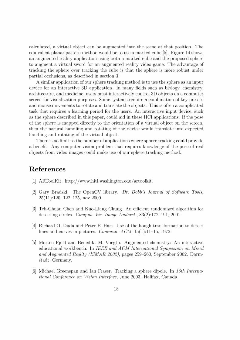
The axis of rotation, R, to align P1 and C1 is computed from the cross product ofthe two unit vectors. The angle of rotation is θ, which is the known angle betweenthe two dots. To explain Figure 9 in more detail, P1 and P2 have been rotated tobecome P1′ and P2′, respectively. Now, P1′ and C1 are aligned, and the new axisof rotation, R, to align P2′ and C2 is the unit vector (C1x,C1y,C1z) through P1′

and C1. Unit vectors through C2 and P2′ are computed using Equation 15. Tocompute the angle of rotation, θ, let the vector u = (ux,uy,uz) be the projectionof (C2x,C2y,C2z) onto R, and the vector v = (vx,vy,vz) be the projection of(P2x

′,P2y′,P2z

′) onto R. Then, manipulating the dot product we have;

|u||v|cos(θ) = (uxvx) + (uyvy) + (uzvz)

θ = cos−1((uxvx) + (uyvy) + (uzvz)

|u||v|) (16)

This rotation aligns the second point. The one item that has yet to be described ishow the virtual sphere is actually rotated by an arbitrary angle, θ, about an arbitraryaxis, R = (Rx,Ry,Rz). The sphere is rotated by rotating the unit vectors thatcorrespond to each of the dots on the sphere surface, one at a time. To rotate a unitvector vi = (x,y, z), the entire space is first rotated about the X-axis to put R inthe XZ plane. Then the space is rotated about the Y-axis to align R with the Z-axis.Then the rotation of vi by θ is performed about the Z-axis, and then the inverse

13

of the previous rotations are performed to return to normal space. This can all beaccomplished by multiplying each unit vector vi by the following rotation matrix; cos(θ) + (1 − cos(θ))Rx

2 (1 − cos(θ))RxRy − Rzsin(θ) (1 − cos(θ))RxRz + Rysin(θ)(1 − cos(θ))RxRy + Rzsin(θ) cos(θ) + (1 − cos(θ))Ry

2 (1 − cos(θ))RyRz − Rxsin(θ)(1 − cos(θ))RxRz − Rysin(θ) (1 − cos(θ))RyRz + Rxsin(θ) cos(θ) + (1 − cos(θ))Rz

2

Once the virtual sphere is aligned to the two chosen points, a score is computed forthis possible orientation. The validity of a given orientation is evaluated based onthe number of visible dots in the perspective projection that align to real dots of thecorrect color on the virtual sphere, as well as how closely the dots align. Visible dotsthat do not align to real dots decrease the score, as do real dots that were not matchedto visible dots. All points are compared using their polar coordinates, and scores arecomputed differently based on the latitude values of the points, since points that arecloser to the center of the sphere projection should contain a smaller error than thosethat are farther from the center. Two points, P1 and C1, are said to match if theangle, θ, between them satisfies the following inequality;

θ < (1 + latc1 ·2

π)(α − β) + β (17)

where α is a high angle threshold for points that are farthest from the center of pro-jection, and β is a low angle threshold for points that are at the center of projection.In our experiments, values of α = 0.4 radians and β = 0.2 radians produces goodresults. Using Equation 17, the number of matched dots is calculated as Nm for agiven orientation. Let Nv be the number of visible dots that are not aligned to realdots, let Nr be the number of real dots that are not matched with visible dots (andyet should have been), and let θi be the angle between the matching pair, i. Thenthe score, σ, is computed as follows;

σ =∑Nm

i=1

[(1 + lati · 2

π)(α − β) + β − θi

]−∑Nv

i=1

[(1 + lati · 2

π)(α − β) + β

]−∑Nr

i=1

[α − (1 + lati · 2

π)(α − β)

] (18)

The orientation that yields the highest score is chosen as the matching orientation forthe sphere in the scene. Figure 10 shows a screenshot of the sphere in an arbitraryorientation with the matching orientation of the virtual sphere shown in the upperleft corner.

3 Occlusion handling

One of the main benefits of our sphere tracking method is that the tracking doesnot fail during partial occlusions. Occlusion is when an object cannot be completely

14

seen by the camera. This normally results from another object coming in betweenthat object and the camera, blocking the view. Section 2.1 explains that the trackingmethod chooses the best-fit circle of the correct hue in the projection of the sceneas the location of the sphere. This means that objects can partially occlude thesphere and yet it may still be chosen as the best-approximated circle. Also, since theminimum enclosing circle is computed from the contour, only the pixels representing180 degrees of the circumference plus one pixel are required in order to determinethe location of the sphere with the correct radius. For this reason, up to half of thesphere projection may be occluded and yet its 3D location will still be computedcorrectly. Furthermore, the tracking process does not require that all of the dots onthe surface of the sphere be visible in order to determine the orientation of the sphere.Since the matched orientation with the best score is chosen, it is possible to occludea small number of the dots and yet still track the orientation correctly. The abilityto correctly handle partial occlusions is very beneficial in a sphere tracking processbecause it allows a person to pick up the sphere and manipulate it with their hands.Figure 11 shows how the sphere tracking does not fail under partial occlusion. In thisscreenshot, the sphere is used in an augmented reality application where a red teapotis being augmented at the location and orientation of the sphere in the scene.

4 Error analysis

The purpose of this section is to determine the accuracy of the sphere tracking methodthat we present. Locating the 3D position of the sphere is not a new technique,however the novelty of this paper lies in the algorithm to determine the 3D orientationof the sphere. Therefore, we will only analyze the performance of that algorithm.

In order to compute an error on the resulting 3D orientation calculation of ourtracking method, the sphere must be manually placed in the scene with a knownorientation. This is a very difficult task because the sphere is a physical object and itis nearly impossible to determine its actual orientation in the scene before performingthe tracking. For this reason, a virtual 3D model of the sphere was built with exactprecision. Then the virtual sphere model was rendered into the scene at a chosenorientation, and the tracking procedure was applied. The actual orientation and thetracked orientation were then compared to determine a tracking error. Specifically,100000 video frames were captured with the virtual sphere inserted at random orien-tations. To avoid additional error due to the weak perspective projection computationdescribed in section 2.1, the virtual sphere was constrained to X and Y values of zero,such that the perspective projection was always in the center of the image plane. TheZ value of the sphere was chosen randomly to simulate different distances from thecamera. The question that remains is how can one 3D orientation be compared to

15

another? It was decided that a particular orientation of the sphere would be definedby the quaternion rotation that transformed the sphere from its standard orientation.A quaternion is a 3D rotation about a unit vector by a specific angle, defined by fourparameters (three for the vector and one for the angle). The two orientations werecompared by analyzing the two quaternions. This produced two errors, one erroron the quaternion axis and one in the angle. The axis error was computed as thedistance between the end points of the two unit vectors which define the quaternions.The angle error was simply the difference between the two scalar angle values. So foreach of the 100000 chosen orientations we have a 6-dimensional vector (4 dimensionsfor the quaternion and 2 for the errors) to describe the tracking error. Visualizingthe error for analysis is a non-trivial task. Even if the errors are analyzed separately,it is still difficult to visualize two 5 dimensional vectors. However, we realize thatthe results of the error analysis will indicate how well the tracking method is able todetermine the best match to the perspective projection of the dots on the surface ofthe sphere. This, in turn, will give some feedback on how well the dots were placedon the sphere and could indicate locations (in polar coordinates) where the dots werenot placed well. So instead of visualizing all four dimensions of a quaternion, thepolar coordinates of the center of the perspective projection were computed for eachorientation. This assumes that a perspective projection of the sphere under any 2Drotation will yield similar errors, which is a reasonable assumption. Now the errorscan be analyzed separately as two 3 dimensional vectors (2 dimensions for the polarcoordinates and one for the error). Figure 12 is a graph of the average error in thequaternion axis over all the polar coordinates, and Figure 13 is a similar graph of theaverage error in quaternion angle. In both graphs, darker points indicate greater errorand white points indicate virtually no error. It is clear to see from Figure 12 thatthe greatest error in quaternion axis is concentrated around the latitude value of −πradians, that is to say, the north pole of the sphere. Figure 13 indicates that the errorin quaternion angle is relatively uniform across the surface of the sphere. Addition-ally, the overall average error in quaternion axis is 0.034, and in quaternion angle is0.021 radians. This analysis shows that the sphere tracking method presented in thispaper has excellent accuracy. These results were obtained on a Pentium 3 processorat 800Mhz using a color Point Grey Dragonfly camera with a resolution of 640x480pixels.

5 Future work

There are a few drawbacks with our sphere tracking method that could benefit fromfuture research. The first problem is with locating the perspective projection ofthe sphere on the image plane. Segmenting the input image by hue value allows

16

continuous tracking under variable lighting conditions. However, if the projection ofanother object with the same hue as the blue ball overlaps the projection of the ballthen the contours of the two objects will merge into a single connected component.This produces an awkward shape in the binary image and tracking will fail. Onesolution to this problem is to segment the input image using standard edge detectiontechniques and then decide which contour most closely represents the sphere, evenunder partial occlusions.

Another problem with the method presented in this paper is that the locationsof the dots on the surface of the sphere were generated randomly and then measuredout and placed on the ball by hand. This technique is prone to human error whichwould lead to errors in the tracking process. A better solution would be to place thedots on the ball first, such that one can visually decide on the locations in order tomaximize the tracking robustness, and then have the system learn the dot locationsfrom the input video.

The final drawback presents the most interesting problem to be solved by futureresearch. The problem is that since the dot locations were generated randomly thereis no way to guarantee that the perspective projection of two different sphere orien-tations are significantly different. If the projection of two different orientations aresimilar then tracking errors will occur. So the question becomes, how can N locationsbe chosen on the surface of a unit sphere such that the perspective projection of thesphere is maximally unique from every viewpoint? However, in practice this situationis rare.

6 Results and applications

We have presented a method to track the 3d position and orientation of a sphere froma real-time video stream. The sphere is a simple blue ball with 32 randomly placedgreen and red dots. Tracking consists of locating the perspective projection of thesphere on the image plane using standard computer vision techniques, and then usingthe projections of the dots to determine the sphere orientation using 3D geometry.

Resolving the 6 DOF pose of a sphere in a real-time video sequence can lead tomany interactive applications. One application that was hinted at in section 3 is inthe field of augmented reality. Augmented reality is the concept of adding virtualobjects to the real world. In order to do this, the virtual objects must be properlyaligned with the real world from the perspective of the camera. The aligning processtypically requires the use of specific markers in the scene that can be tracked in thevideo, for instance, a 2d pattern on a rigid planar object [1]. An alternate way toalign the real world and the virtual objects is to use the marked sphere and trackingmethod described in this paper. Once the location and orientation of the sphere is

17

calculated, a virtual object can be augmented into the scene at that position. Theequivalent planar pattern method would be to use a marked cube [5]. Figure 14 showsan augmented reality application using both a marked cube and the proposed sphereto augment a virtual sword for an augmented reality video game. The advantage oftracking the sphere over tracking the cube is that the sphere is more robust underpartial occlusions, as described in section 3.

A similar application of our sphere tracking method is to use the sphere as an inputdevice for an interactive 3D application. In many fields such as biology, chemistry,architecture, and medicine, users must interactively control 3D objects on a computerscreen for visualization purposes. Some systems require a combination of key pressesand mouse movements to rotate and translate the objects. This is often a complicatedtask that requires a learning period for the users. An interactive input device, suchas the sphere described in this paper, could aid in these HCI applications. If the poseof the sphere is mapped directly to the orientation of a virtual object on the screen,then the natural handling and rotating of the device would translate into expectedhandling and rotating of the virtual object.

There is no limit to the number of applications where sphere tracking could providea benefit. Any computer vision problem that requires knowledge of the pose of realobjects from video images could make use of our sphere tracking method.

References

[1] ARToolKit. http://www.hitl.washington.edu/artoolkit.

[2] Gary Bradski. The OpenCV library. Dr. Dobb’s Journal of Software Tools,25(11):120, 122–125, nov 2000.

[3] Teh-Chuan Chen and Kuo-Liang Chung. An efficient randomized algorithm fordetecting circles. Comput. Vis. Image Underst., 83(2):172–191, 2001.

[4] Richard O. Duda and Peter E. Hart. Use of the hough transformation to detectlines and curves in pictures. Commun. ACM, 15(1):11–15, 1972.

[5] Morten Fjeld and Benedikt M. Voegtli. Augmented chemistry: An interactiveeducational workbench. In IEEE and ACM International Symposium on Mixedand Augmented Reality (ISMAR 2002), pages 259–260, September 2002. Darm-stadt, Germany.

[6] Michael Greenspan and Ian Fraser. Tracking a sphere dipole. In 16th Interna-tional Conference on Vision Interface, June 2003. Halifax, Canada.

18

[7] Euijin Kim, Miki Haseyame, and Hideo Kitajima. A new fast and robust circleextraction algorithm. In 15th International Conference on Vision Interface, May2002. Calgary, Canada.

[8] Robert A. McLaughlin and Michael D. Alder. The hough transform versus theupwrite. IEEE Trans. Pattern Anal. Mach. Intell., 20(4):396–400, 1998.

[9] Gerhard Roth and Martin D. Levine. Extracting geometric primitives. CVGIP:Image Underst., 58(1):1–22, 1993.

[10] Reza Safaee-Rad, Ivo Tchoukanov, Kenneth Carless Smith, and Bensiyon Ben-habib. Three-dimensional location estimation of circular features for machinevision. Transactions on Robotics and Automation, 8(5):624–640, 1992.

[11] Y.C. Shiu and Shaheen Ahmad. 3d location of circular and spherical features bymonocular model-based vision. In IEEE Intl. Conf. Systems, Man, and Cyber-netics, pages 567–581, 1989.

[12] L. Xu, E. Oja, and P. Kultanen. A new curve detection method: randomizedhough transform (rht). Pattern Recogn. Lett., 11(5):331–338, 1990.

[13] H. K. Yuen, J. Illingworth, and J. Kittler. Detecting partially occluded ellipsesusing the hough transform. Image Vision Comput., 7(1):31–37, 1989.

19

(a)

(b)

(c)

Figure 8: Rotation to align the first point. a) standard view; b) with sphere removedfor visualization; c) rotated view for clarity.

20

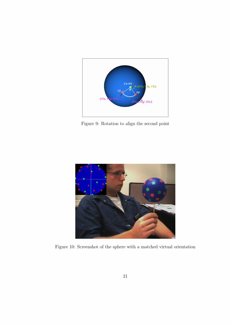
Figure 9: Rotation to align the second point

Figure 10: Screenshot of the sphere with a matched virtual orientation

21

(a) (b)

(c) (d)

Figure 11: Handling partial occlusions. a) un-occluded input; b) un-occluded track-ing; c) occluded input; d) occluded tracking.

22

Figure 12: Analysis of error on quaternion axis

Figure 13: Analysis of error on quaternion angle

23

Figure 14: Augmented reality application of the sphere tracking method

24