1

NSF Energy Project: Overview

"Decision Models for Bulk Energy Transportation Networks"

NSF Grant No. 0527460: 9/1/05-8/31/09

Final Report November 29, 2009

PI/Co-PIs:

James McCalley (EE), Sarah Ryan (IE), Stephen Sapp (Sociology), Leigh Tesfatsion (Economics)

Current Research Assistants: Natalia Frishman (PhD Sociology),

Yang Gu (PhD EE), Eduardo Ibanez (EE), Abhishek Somani (PhD Econ), Yan Wang (PhD Econ)

Graduated Research Assistants

Previously Supported: Ana Quelhas (PhD EE), Esteban Gil (PhD EE),

Junjie Sun (PhD Econ), Yan Wang (MS IE)

NSF Project Home Page: http://www.econ.iastate.edu/tesfatsi/NSFEnergy2005.htm

2

Table of Contents Context................................................................................................................................ 3 Objective ............................................................................................................................. 3 A. Structural Model ............................................................................................................ 4

A.1 Modeling catastrophic events................................................................................... 5 A.1.1: Modeling Improvements:................................................................................. 5 A.1.2 Data gathering ................................................................................................... 7

References for Section A.1 ........................................................................................... 10 A.2 Treatment of uncertainty........................................................................................ 10

A.2.1 Data gathering for 2006 NEES model: ........................................................... 11 A.2.2 Stochastic modeling: ....................................................................................... 11 A.2.2 Uncertainty analysis: To be completed by JDM…......................................... 11

References for Section A.2 ........................................................................................... 12 A.3 Use for economic planning studies ........................................................................ 12

B. Agent-Based Behavioral Model ................................................................................... 13 B.1 Key Features........................................................................................................... 13 B.2 Key Findings .......................................................................................................... 15 References for Section B .............................................................................................. 20

C. Model integration ......................................................................................................... 28 References for Section C: ............................................................................................. 29

D. Impediments to transmission line investment.............................................................. 29

3

Context This work targets what we call the National Electric Energy System (NEES), which is comprised of physical infrastructure, industrial and governmental organizations, individual and corporate decision-making entities, and associated information processing systems for • Electric generation and bulk transmission systems • Natural gas production and pipeline systems • Coal production and rail/barge transportation systems • Water reservoirs and hydroelectric production systems • Influence of carbon dioxide, sulfur dioxide, and nitrogen oxide constraints • Markets and market agents which comprise economic systems for bulk energy trading

Objective The objective of this research is to develop two complementary and related classes of decision models, a structural model & a behavioral model, for the ultimate purpose of addressing the following issues: National Scale (federal government, NERC): (1) Possible improvements in energy flow patterns (2) Effects of catastrophic events (3) Detection of physical infrastructure weaknesses (4) Detection of weaknesses in institutional arrangements (5) Infrastructure enhancements to improve performance (6) Effects of environmental regulations on energy system performance Regional Scale (regional independent system operator): (1) Effects of market design on market (energy system?) performance (2) Sensitivity of market performance to system shocks (3) Potential improvements in market design Local Scale (local electric utility company): (1) Effects of changes in raw fuel production and transportation on the returns from investing in specific types of plants at specific locations (2) Response of energy buyers and sellers to potential new policies designed to improve transparency and ease of trade We are developing two complementary and related classes of decision models, a structural model and an agent-based behavioral model, as illustrated in Fig. 1. Progress on the structural model is described in Section A. Progress on the behavioral model is described in Section B. Progress on integration of the two models is described in Section

4

C. An effort to understand impediments to transmission line investment is described in Section D.

Behavioral Model

Regional Electricity

market

Structural Model

E

Fig. 1: Interaction of structural and behavioral model

A. Structural Model The structural model is based on a generalized network flow model that captures the gas, coal, and water production, storage, and transportation systems and the electricity generation and transmission systems, at a national level. The top part of Fig. 1 provides conceptual illustration of the structural model.

5

The structural model simulates the national energy system. Simulation times are in the order of few months to several years. An important element of the structural model is its ability to integrate the four different energy subsystems (electric, coal, gas, water) in a single model. A key model attribute that facilitates this within our network flow model is the ability to model different portions of the energy system with varying levels of time-step granularity. Figure A.1 illustrates. Input data to the model includes topology (nodes, arcs), supply and demand at gas and coal supply points and electric demand points, respectively, per unit energy flow cost along each arc, and arc capacities and efficiencies, all at each time t. We developed aggregated topologies to represent the national US energy system.

Fig. A.1: Varying Time-Step Modeling for Coal, Gas, Electricity

• The model is solved as the generalized network simplex algorithm (a specialized linear program), which is extremely efficient, capable of handling very high-dimensional problems. We use CPLEX to implement the solutions.

There have been three main areas of progress regarding the structural model: • Modeling catstrophic events, as described in section A.1. • Representing uncertainty, as described in section A.2. • Use for economic planning studies, as described in section A.3.

A.1 Modeling catastrophic events We used the 2005 Katrina/Rita hurricane events to motivate our effort to model and study catastrophic events on the NEES. To this end, several modeling improvements were made relative to what was done in our previous work [A1-1, A1-2], a very large data gathering effort was performed, and valiadation studies were implemented. This work is reported in [A1-3]. This work is supervised by Dr. McCalley.

A.1.1: Modeling Improvements:

6

The modeling improvements are summarized below: 1. Modeling the demand not served: The use of network linear programming to obtain a

minimum-cost pattern of energy movements makes the implicit assumption that the model is able to satisfy the demand. However, due to the effects of a major contingency, the network simplex algorithm used for simulation may not be able to find a feasible solution to the optimization problem. In other words, it may be the case that there is not feasible flow able to either locally or globally satisfy the demand either of electricity or of coal and natural gas for uses other than electricity generation. To overcome the possibility of infeasible solutions, some adjustments to the network model are necessary. The solution implemented is to add a dummy supply node connected to all the electricity and natural gas transshipment nodes by arcs having unlimited capacity in order to satisfy any possible demand.

2. Modeling sequential decisions: In the network model developed in our previous work [A1-1], decisions variables (flows) for every time step are determined simultaneously, that is, the optimization process treats the entire multi-time-period network as a single static network and finds the optimal way to satisfy the demands on that network. This approach implies prior knowledge on any changes in the network parameters, such as the reduction on the capacity of one or more arcs as a result of a disruption. A simple approach to address this issue consists of decoupling the network so that the pre and post contingency decisions are independent. This independence can be achieved by eliminating the arc corresponding to the storage carried out from the period immediately before the contingency and the period immediately after the contingency, and adjusting the demands on the corresponding storage nodes accordingly.

3. Improvements in the demand model: There were two improvements: a. Elasticity: The energy demand is highly inelastic with respect to prices, so the

assumption of inelastic demand as considered in our previous model is appropriate under normal operating conditions. However, under the effects of a major contingency, congestion may lead to large price peaks either locally or globally, and the prices may increase so much that the assumption of demand inelasticity may not hold true. A practical consideration is that with elastic demand the network problem will no longer be linear since the value of an elastic demand would depend on the dual solution of the generalized minimum cost flow problem and thus the optimal solution can not be obtained in a single iteration as done in our previous work. A demand response mechanism was implemented as part of an iterative process to take into account the effect of elasticity. The first iteration uses an initial estimate for the demands at the transshipment node, then solves the problem using the network simplex algorithm, and finally, determines a first estimate for the nodal prices from the dual solution. Before the second run of the network simplex algorithm, the demand response mechanism takes place and new demands are calculated by computing the product of the percent increase in nodal prices (with respect to a base case) and the values for elasticity. With the new values for the demands, a new solution is obtained by using the network simplex algorithm. The process is repeated until convergence.

7

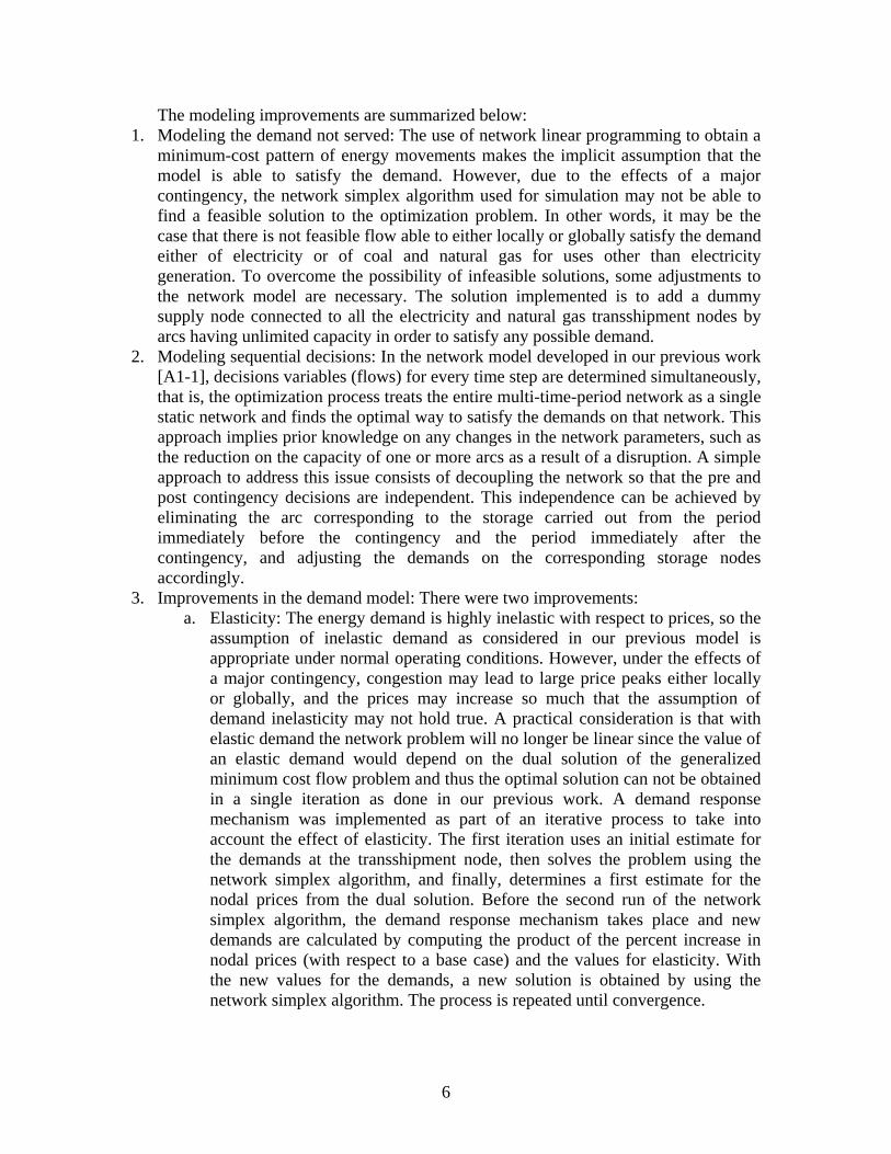
b. Decomposition by demand levels: Simulations in the network model provide results that are aggregated for each time step. That is, energy flows and nodal prices within a given time step are aggregated into a single value, and any variability in the system variables occurring within a time step is lost. The time step used in previous work (a month) might not reflect some effects and interactions that may be important when studying the effects of disruptions, like for example system congestion or price spikes that are especially noticeable during periods of high load. Moreover, since gas fired generation is more expensive than coal-fired generation, typically many natural gas power plants do not operate continuously but only on periods of high demand. If the model is not able to represent periods when high demand occurs, then in the simulation results some of the more expensive generating units will never be used. The consequences of not modeling variation of load level are inaccuracy on the calculation of electricity prices, congestion levels, and fossil fuel use. To solve this issue, the demand for each month and for each node is decomposed as illustrated in Figure A.2.

Figure A.2: Load decomposition

4. DC-Flow representation: In previous work, electric transmission was represented

using a transportation network, i.e., Kirchoff’s laws were not enforced. We have addressed this modeling weakness by implementing a DC power flow representation within the overall transportation model. This modeling improvement is reported in [A1-4].

A.1.2 Data gathering Data was gathered for the electric, natural gas, and coal bulk production and transportation sub-systems. The data reflects the hurricane’s effects in terms of changes in production, transportation, storage, and prices of different energy forms. Where

8

possible, data was gathered to reflect conditions given months or years before and for the months following the hurricanes. Data sources include daily situation reports by the Department of Energy’s Office of Electricity Delivery and Energy Reliability (OE), Energy Information Administration (EIA), Louisiana Public Services Commission, North America Electric Reliability Council (NERC), Mineral Management Service (MMS), Office of Pipeline Safety (OPS), Pipeline and Hazardous Materials Safety Administration (PHMSA), and on-site interviews, news releases, and financial releases offered by energy companies affected by the hurricanes. These data are summarized at http://home.eng.iastate.edu/~jdm/katrina/ and reported in part in []. A.1.3 Validation studies Validation of an earlier version of the NEES network model using 2002 data was carried out and reported in [2], where the reference case was designed with the actual configuration of generation and loads reported on a monthly basis for the year 2002. That is, coal-fired net generation and gas-fired net generation for each region and for each time step were fixed, together with the total emissions for 2002. This approach validated the model’s ability to replicate fuel production and transportation to the generators. This validation effort reported aggregated simulation results, with annual total flows and annual average prices. In the more recent validation effort using the 2005 data (as described in the previous section), instead of fixing all generation as in the 2002 case, only the loads and the total coal-fired net generation per month and per NERC region were fixed. Therefore optimization was performed on the coal, natural gas, and electricity flows. This reference case used for validation is less restrictive since it allows more freedom for the variables to change, especially the variables in the natural gas subsystem which were directly affected by the hurricanes in 2005. The purpose of this validation scheme is to test the ability of the model to reflect the effects of hurricanes Katrina and Rita in the U.S. energy system, and to capture how these effects (in terms of energy prices) propagated across time, space, and subsystems characterizing bulk energy transportation. Results of the simulation are compared to the corresponding actual values in Table A.1.

TABLE A.1: VALIDATION RESULTS FOR 2005 DATA

9

Result Model Actual Difference

NG total production [Bcf] 17,200 18244* -5.52%

NG imports from Canada [Bcf] 4,280 3,700 15.56%

NG production plus imports [Bcf] 21,480 21,944 -2.11%

Coal production [billion short ton] 1.08 1.128 -4.30%

NG consumed by electric sector [Bcf] 5,936 5,869 1.15%

NG consumed for uses other thanpower [Bcf] 14,500 14,500 0%

Gas-fired net generation [MWh] 712.63 757.97 -5.98%

Coal consumed by electric sector[billion short ton] 1 1.038 -3.66%

Cost of NG for electric power [$/Mcf] 9.02 8.49 6.20%

Cost of coal for electric power[$/short ton] 29.61 31.22 -5.20%

Electric energy price [$/MWh] 78.5 81.4 -3.60%

* Dry production Another result of this study is illustrated in Fig. A.3, which shows price variation throughout the nation for the remaining four months of 2005 following the occurrence of the hurricanes. Although the different curves look similar to each other, there are some noteworthy differences, as illustrated in Fig. A.4, which shows the percentage increase in natural gas nodal prices in each month, by region, following the hurricanes. Figure A.3 shows that the node with the larger increase was the Southwest natural gas transshipment node (representing the gulf region and the southwest US), which is reasonable considering that it is the node directly affected by the hurricanes. While still affected in terms of relative increase in nodal prices, the less affected nodes were the Midwest and Northeast nodes, which are the only natural gas transshipment nodes not directly connected by an arc to the Southwest node. This suggests the reasonable indication that the effects of a disruption are more severe in the nodes that are closer to it.

Figure A.3: Effect of hurricanes Katrina and Rita in natural gas nodal prices

10

0%

5%

10%

15%

20%

25%

30%

35%

40%

Sep Oct Nov DecMonth (2005)

Per

cent

age

of in

crea

se (%

)

Western

CentralMidwest

Northeast

Southwest

Southeast

Fig. A.4: Percentage of increase in natural gas nodal price with the hurricanes

References for Section A.1 [A1-] A. Quelhas, E. Gil, J. D. McCalley, and S. M. Ryan, “A Multiperiod Generalized Network Flow Model of the US Integrated Energy System: Part I—Model Description,” Power Systems, IEEE Transactions on, vol. 22, pp. 829-836, 2007. [A1-2] A. Quelhas and J. D. McCalley, “A Multiperiod Generalized Network Flow Model of the US Integrated Energy System: Part II—Simulation Results,” Power Systems, IEEE Transactions on, vol. 22, pp. 837-844, 2007. [A1-3] E. Gil and J. McCalley, “A US Energy System Model for Disruption Analysis: Validation Using Effects of 2005 Hurricanes,” under review. [A1-4] Y. Gu, E. Ibanez, and J. McCalley, “Uncertainty representation in integrated energy systems,” under review for the 11th International Conference on Probabilistic Methods Applied to Power Systems, June 2010, Singapore.

A.2 Treatment of uncertainty

Three main thrusts characterized this effort. In the first, a new set of data was gathered to model the 2006 NEES. In the second, a stochastic programming approach was implemented to capture influential uncertainties in the model. These two thrusts are described in Sections A.2.1 and A.2.2 below and published in [A1-1, A2-2]. This work is

11

supervised by Dr. Ryan. In the third, uncertainty representation is assessed using Monte Carlo simulation. This work is supervised by Dr. McCalley.

A.2.1 Data gathering for 2006 NEES model: The entire data set for the bulk energy transportation network was comprehensively updated for the year 2006. This is a very labor-intensive process that requires accessing data from multiple online sources, followed by substantial processing to compute model parameters in the required format. We systematically verified those 2002 data that were still available, carefully documented the sources and processing involved, and created the corresponding 2006 data set. Some of the electricity subsystem topology changed due to reorganization of NERC regions between 2002 and 2006.

A.2.2 Stochastic modeling: We investigated computational and approximation methods to improve the tractability of a stochastic program for incorporating fuel price and demand uncertainty in the bulk energy transportation network. These include decomposition, scenario aggregation and reduction, scenario sampling, and various combinations of these techniques. We used duality and complementarity concepts in stylized examples to illuminate reasons for the unexpected finding that uncertainty in natural gas prices could increase the proportion of electricity generated from natural gas rather than coal. We conducted a closer examination of the fuel network data to understand why some nodal prices for coal were higher than those for natural gas in the original 2002 data set. Compared to the expected value solution from the deterministic model, the recourse solution found from the stochastic model for 2002 has higher total cost, lower natural gas consumption and less subregional power trade but a fuel mix that is closer to the actual. The comparisons are qualitatively similar but muted in the 2006 case. To improve computational tractability with large numbers of scenarios in the stochastic model, we developed a heuristic importance sampling scheme that integrates well with the rolling horizon solution procedure. This development permitted solution of the full monthly model (without quarterly aggregation previously introduced) and confirmed the qualitative comparison between solutions of the stochastic and deterministic versions of the problem. We also developed a structural scenario reduction method that selects scenarios to retain based on their impact on the first-stage decisions. This accomplished considerable problme size reduction and maintained accuracy of the recourse solutions with less computational effort than general scenario reduction.

A.2.3 Uncertainty analysis using Monte Carlo The uncertainties which are considered in this section are as follows: • Uncertainty in fuel prices • Uncertainty in availability of generation and transmission facilities • Uncertainty in capacities of fuel transportation facilities

12

The algorithm to analyze the operation of integrated energy system using Monte Carlo simulation method is given below: 1) Determine the forecasts of prices of each kind of fuel resources and the load levels. 2) Determine the probability density functions for all of the random uncertainties assessed. For each time step, we obtain:

• The variances of natural gas and oil prices • The forced outage rates of generating units and transmission lines • The variances of normally distributed random input associated with maximum

capacities of transmission lines 3) Generate a number from the probability density functions of each random parameter and compute the value of its corresponding parameters. For parameters associated with fuel prices or maximum flow capacities in fuel transportation lines, we update maximum capacities for each time step; for parameters about availabilities of generating units or transmission lines, we compare the number generated with the standard uniform distribution with forced outage rate of one unit. 4) Run the production cost model of integrated energy system using the inputs and parameters in steps 1, 2 and 3 and save the results. 5) Repeat steps 3 and 4 a large number of times. 6) Analyze the results using statistical methods, e.g. fitting a probability density function to the LMPs generated in step 5 or calculate the mean and variance of LMPs. This method was implemented on a test system and results are reported in [A2-3].

A.3 Use for economic planning studies There has been significant interest over the past 3-4 years in enhancing the planning function so that infrastructure investment is not motivated only by future reliability weaknesses but also by economic opportunity. Thus, we have identified and tested several metrics for identifying such transmission investments. These include congestion rents, branch shadow price, and reduced cost (profit per unit of flow). We have implemented such an economic planning procedure on a test system and reported results in [A2-3].

References for Sections A.2 and A.3 [A2-1] S. Ryan and Y. Wang, “Efficient methods for solving a large-scale multistage stochastic program,” INFORMS Annual Meeting, Seattle, November 2007 [A2-2] Y. Wang and S. Ryan (2009). Effects of uncertain fuel costs on optimal energy flows in U.S. Submitted to Energy Systems, under review. [A2-3] Y. Wang and S. Ryan (2009). Comparison of Efficient Methods for Solving a Large-Scale Multistage Stochastic Program. Proceedings of the Industrial Engineering Research Conference, Miami, FL, May 2009. [A2-3] Y. Gu, E. Ibanez, and J. McCalley, “Uncertainty representation in integrated energy systems,” under review for the 11th International Conference on Probabilistic Methods Applied to Power Systems, June 2010, Singapore.

13

B. Agent-Based Behavioral Model In April 2003 the U.S. Federal Energy Regulatory Commission (FERC) proposed a wholesale power market design for U.S. energy markets featuring the ISO/RTO management of a two-settlement system (real-time and day-ahead markets) with locational marginal pricing to handle congestion on the transmission grid. Over 50% of generation capacity in the U.S. today is now operating under some variant on this design. The primary objective of this part of our NSF project has been to develop AMES, an agent-based wholesale power market test bed capturing core aspects of FERC’s market design, as a commercial overlay for the NEES structural network model. The first version of AMES (V1.31) was released as open-source software at the IEEE PES General Meeting in June 2007. More powerful versions of AMES have since been released, most recently V2.05 formally presented at the IEEE PES General Meeting in July 2009. This work, supervised by Dr. Tesfatsion, is published in the references [B-1]-[B-15]. There have also been two software releases corresponding to this work [B-16, B-17].

B.1 Key Features As indicated in Fig. B.1, AMES models wholesale power market traders as learning agents capable of autonomous goal-seeking behaviors and strategic response to the incentives intentionally or unintentionally built into FERC’s market design. The wholesale power market operates over a transmission grid subject to congestion effects. The ISO handles congestion by the inclusion of congestion cost components in locational marginal prices derived from DC optimal power flow solutions.

Fig. B.1: AMES Modular and Extensible Architecture

14

The activities of the ISO on a typical day D are schematically depicted in Fig. B.2. The indicated timing is adopted from the MISO.

Fig. B.2: AMES ISO activities during a typical day D

As depicted in Fig. B.3, AMES is currently implemented by means of three main Java modules: a learning module for traders; a DC-OPF module for the determination of commitment/LMP solutions for the day-ahead (and real-time) markets; and a graphical user interface (GUI) with separate screens for carrying out many important user functions (e.g., case study creation and modification, customizable output table and chart displays, and setting of stopping rules and other simulation control aspects).

15

Fig. B.3: Illustrative depiction of AMES dynamics on a typical day D for a 5-bus test

case in the absence of shocks or disturbances

B.2 Key Findings First, the AMES wholesale power market test bed has been used to systematically investigate the effects of changes in GenCo learning parameters, demand-bid price sensitivities, and GenCo supply-offer price caps on LMP separation and volatility over time in both 5-bus and 30-bus test cases. The primary objective has been to gain a more fundamental understanding of how learning, network externalities and GenCo pivotal and marginal supplier status interact to determine the distribution of LMPs both across the grid (separation) and over time (volatility). Our key findings to date are as follows: • Using only simple stochastic reinforcement learning, generation companies (GenCos)

quickly learn to tacitly collude on reported marginal cost functions (supply offers) for the day-ahead market that are higher than their true marginal cost functions, resulting in higher locational marginal prices (LMPs).

• This result holds for all tested levels of price sensitivity for the bid-in demand by load-serving entities (LSEs), ranging from 100% fixed demand (no price sensitivity) to 100% price sensitivity.

• However, LMPs are substantially higher the greater the percentage of fixed to price-sensitive demand.

• Supply-offer price caps, i.e., upper bounds imposed on the GenCos’ reported marginal cost functions (supply offers), can decrease average LMP.

• However, the imposition of strongly binding supply-offer price caps can lead to increased LMP spiking and volatility around peak demand hours.

Second, the AMES test bed (for dynamic 5-bus and 30-bus test cases) has been used to explore the market efficiency implications of the net surplus (congestion rents)

16

collected and redistributed by ISOs in restructured wholesale power markets with grid congestion managed by LMP. The AMES simulation findings suggest that these ISO net surplus extractions can be substantial and tend to increase in conditions unfavorable to market efficiency. ISO yearly reports for PJM and other energy regions indicate that actual ISO net surplus extractions are in fact substantial. A practical implication is that a more transparent public oversight of all net surplus extractions and uses in wholesale power markets operating under LMP would be publicly prudent because these extractions are not structurally well-aligned with market efficiency objectives. Third, the AMES test bed has been used to investigate strategic capacity withholding by GenCos in restructured wholesale power markets using dynamic 5-bus test cases. Real-world restructured wholesale power markets are sequential open-ended games for GenCos, so they have a learning-to-learn issue. Consequently, as a preliminary step, the GenCos' learning methods are calibrated to their decision environment. Experiments are then conducted to investigate GenCo economic and physical capacity withholding both separately and in combination. Results indicate that economic capacity strongly dominates physical capacity withholding in terms of permitting GenCos to substantially increase their net earnings. Our key findings from these three types of experiments are more fully explained and illustrated in the following summary paragraphs.

B.3: LMP Separation and Volatility Experiments One key treatment factor considered in these experiments is the ratio R of maximum potential price-sensitive demand to maximum potential total demand. The construction of the R ratio is illustrated in Fig. B.4.

Fig. B. 4: Construction of R ratio for measuring relative demand-bid price

17

A second key treatment factor is a supply-offer price cap. This price cap is an upper bound imposed on the marginal cost functions that GenCos can report to the ISO for the day-ahead market as part of their supply offers; it is not a cap on LMPs per se. Table B.1 reports experimental findings for average outcomes under alternative settings for the R ratio (relative demand-bid price sensitivity) in the absence of a supply-offer price cap and with no GenCo learning. Table B.2 reports results for a repeat of these R experiments for the case in which GenCos learn to report strategic supply offers to the ISO over time.

Table B.1: Average effects of R changes with no supply-offer price cap and no GenCo learning as R varies from 0.0 (no price-sensitive demand)

to R=1.0 (100% price-sensitive demand)

As seen in Table B.1, in the absence of GenCo learning an incremental increase in R starting from the benchmark case R=0.0 (no price-sensitive demand) and terminating at R=1.0 (100% price-sensitive demand) has the usual intuitively-expected effects. Average LMP, average total demand, average operating costs, and the average Lerner Index (LI) measurement for market power all monotonically decline with increases in R. Indeed, except for the presence of binding operating-capacity constraints on GenCos for low R ratio values (i.e., when average total demand is relatively high) and congestion on branch 1-2 leading to LMP separation and out-of-merit-order commitment, all of the average LI outcomes reported in Table B.1 would be zero. GenCos have no learning capabilities and are reporting their true cost and capacity conditions to the ISO each day; they are not making any deliberate efforts to exercise market power. Comparing the no-learning Table B.1 results to the results with GenCo learning reported in Table B.2, it is seen that GenCo learning has strong effects on average outcomes. With GenCo learning, average LMP, average operating costs, and average LI are all dramatically higher for every level of R even though average total demand is lower. The reason is that the profit-seeking GenCos quickly learn to tacitly collude on higher-than-true reported marginal costs even when demand bids are fully price sensitive (R=1.0) and GenCos are competing for limited demand.

18

Table B.2: Average effects of R changes (with standard deviations) with no supply-offer price cap and with GenCo learning

Table B.3 reports average LMP outcomes under four alternative scenarios for PCap, the supply-offer price cap. For the subsequent interpretation of these findings, it is important to recall that PCap is a price cap on GenCo-reported marginal costs and not on LMPs per se. LMPs can separate from all GenCo-reported marginal costs in the presence of binding GenCo operating constraints and branch constraints, thus PCap is not necessarily an upper bound on LMPs.

Table B.3: Average LMP response (with standard deviations) to changes in PCap, the supply-offer price cap, for R=0.0 (no price-sensitive demand)

As intuitively expected, with GenCo learning, average LMP in TableB.3 monotonically decreases as PCap is decreased in increments from an effectively infinite value (No Price Cap) to a low value ($80/MWh). Due to learning and network effects, however, the relationship between PCap and LMP outcomes is more complicated than indicated by this average LMP effect. In particular, note in Table B.3 that average LMP with no price cap is $70.10/MWh whereas average LMP for PCap=$120/MWh is only $65.72/MWh. This finding indicates that the high PCap level $120/MWh is binding on the GenCos' reported marginal costs even though this PCap level is substantially higher than the resulting value $65.72/MWh for average LMP. A similar comment holds for the remaining two PCap levels.

19

The explanation for this finding is that the distribution of LMPs across the 24 hours of a day can exhibit substantial fluctuations that are obscured when only daily average LMP outcomes are considered. In particular, the maximum LMP value attained during peak demand hours can be substantially higher than average LMP calculated across all 24 hours. Thus, the imposition of a price cap can be a binding constraint on GenCo-reported marginal costs during peak demand hours even if not in other hours. Since GenCos are only permitted to report one supply offer per day, a binding constraint on reported marginal costs during peak demand hours translates into a binding supply-offer constraint for every hour. Finally, as shown in Figs. B.6 and B.7 for the tested scenario with no demand-bid price sensitivity (R=0.0) and with GenCo learning, the introduction of a binding PCap level can in some cases induce more fluctuations in hourly LMPs while in other cases fluctuations are dampened. In particular, the introduction of the strongly binding PCap level $80/MWh increases both volatility and spiking whereas the introduction of the more moderately binding PCap levels $120/MWh and $100/MWh have the opposite effect.

Fig. B.5: Average hourly LMP response to changes in PCap, the supply-offer price cap, with R=0.0 (no price-sensitive demand) and with GenCo learning

Fig. B.6: Average LMP volatility and spiking under varied supply-offer price caps

with R=0.0 (no price-sensitive demand) and with GenCo learning

20

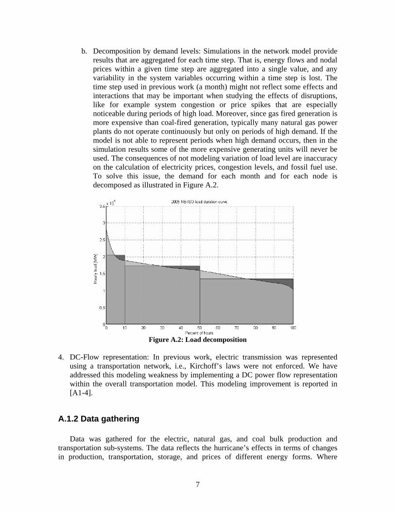
B.4: ISO Net Surplus Extraction Experiments This subsection reports on experiments conducted using dynamic 5-bus and 30-bus test cases to explore the market efficiency implications of the net surplus (congestion rents) collected and redistributed by ISOs in day-ahead energy markets with grid congestion managed by locational marginal pricing (LMP); see Fig. B.7. Demand price sensitivity and generator learning capabilities are taken as treatment factors.

Fig. B.7: Extraction of ISO net surplus in day-ahead energy markets under

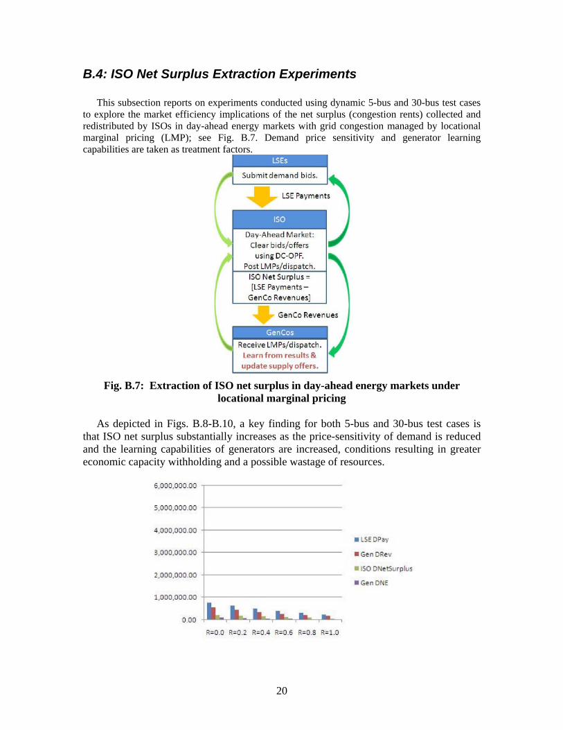
locational marginal pricing As depicted in Figs. B.8-B.10, a key finding for both 5-bus and 30-bus test cases is that ISO net surplus substantially increases as the price-sensitivity of demand is reduced and the learning capabilities of generators are increased, conditions resulting in greater economic capacity withholding and a possible wastage of resources.

21

Fig. B.8: Benchmark (no learning) 5-bus test case: Typical LSE daily payments, GenCo daily revenues, ISO daily net surplus, and GenCo daily net earnings

Fig. B.9: Dynamic 5-bus test case with learning GenCos: Mean LSE daily payments, GenCo daily revenues, ISO daily net surplus, and GenCo daily net

earnings on day 1000 as R varies from R=0.0 to R=1.0.

Fig. B.10: 30-Bus Test Case: Mean ISO net surplus extractions on Day 1000

for R=0.0 (100% fixed demand) Comparisons of empirical ISO/RTO day-ahead market net surplus (congestion rent) extractions with our simulation findings are not straightforward. For example, the congestion costs, congestion charges, and net congestion revenues data presented in the ISO/RTO state-of-the-market and market monitoring reports are in highly aggregated dollar form, and in some cases the explanation of calculation procedures is not fully given. In addition, these dollar amounts should ideally be normalized in some consistent fashion across ISO/RTOs to correct for the size differences among ISO/RTO markets. Despite these difficulties, the following empirical data suggest that ISO net surplus extractions can indeed be large in ISO-managed day-ahead markets: • From PJM 2008 report: Day-ahead congestion cost (ISO net surplus) is $2.66

billion, approximately 7% of total PJM billings listed as $34.3 billion. • From CAISO 2008 report: Day-ahead inter-zonal congestion charges are $176

million. • From ISO-NE 2008 report: Combined 2008 Net Congestion Revenue for real-time

and day-ahead markets is $121 million.

22

• From MISO 2007 report: The congestion cost for day-ahead market is $633 million and the total congestion cost combining both day-ahead and real-time markets is $713 million.

Power market researchers recognize that an important goal of market design is to ensure the structural alignment of participant objectives with socially desirable outcomes, thus reducing the need for oversight of participant behaviors. The main conclusion drawn from the findings reported in this subsection is that net surplus extractions are not structurally well-aligned with market efficiency objectives in ISO-managed wholesale power markets operating under LMP. The immediate practical import is the desirability of encouraging more transparent public reporting and oversight of net surplus extractions and uses to maintain the confidence of both market participants and the public at large.

B.5: Economic and Physical Capacity Withholding Experiments This subsection describes experimental findings for a dynamic 5-bus test case implemented via the AMES Wholesale Power Market Test Bed to investigate strategic capacity withholding by GenCos in restructured wholesale power markets. The strategic behaviors of the GenCos are simulated by means of a simple stochastic reinforcement learning algorithm. The learning GenCos attempt to improve their net earnings over time by strategic selection of their reported supply offers. This strategic selection can involve economic capacity withholding (reporting of higher-than-true marginal costs), physical capacity withholding (reporting of lower-than-true maximum operating capacity), or combinations of the two. As indicated in Table B.4, our findings indicate that the relatively large and expensive GenCo 3 (located at the load-pocket Bus 3) attains much higher mean net earnings relative to the benchmark no-learning case when it is able to exercise economic capacity withholding. This turns out to be the case whether or not GenCo 3 is also able to engage in physical capacity withholding. Conversely, although GenCo 3’s mean net earnings increase when it exercises only physical capacity withholding, increasingly so for successively smaller settings for its minimum possible reported maximum capacity (MPRMCap) value, these gains are substantially smaller. Table B.4: Dynamic 5-bus test case: Mean outcomes (with standard deviations) on day 1000 for GenCo daily net earnings and reported supply offers when GenCo 3

can learn to exercise economic capacity withholding.

23

As indicated in Table B.5, joint learning experimental findings for GenCo 3 and the relatively large but inexpensive baseload GenCo 5 demonstrate that both GenCos attain much higher mean net earnings relative to the benchmark no-learning case when they exercise economic capacity withholding alone or a combination of economic and physical capacity withholding. Conversely, GenCo 3 and GenCo 5 achieve much smaller gains in mean net earnings when they only exercise physical capacity withholding. Also, GenCo 3’s favorable load-pocket location gives it more market power than GenCo 5 because it is a pivotal supplier in almost every hour of every run. GenCo 5’s best capacity withholding choices are affected by GenCo 3’s choices, but GenCo 3’s best capacity withholding choices are largely unaffected by the choices of GenCo 5. Table B.5: Dynamic 5-bus test case: Mean outcomes (with standard deviations) on

day 1000 for GenCo daily net earnings and reported supply offers when both GenCo 3 and GenCo 5 can learn to exercise economic capacity withholding.

24

Figure B.11 depicts GenCo 3’s actual reported maximum capacity versus its optimal reported capacity (ORCap) under a range of different MPRMCap settings for GenCo 3. More precisely, for each given MPRMCap setting, ORCap gives the best possible capacity value that GenCo 3 could report to the ISO in the sense that this reporting leads to the highest mean daily net earnings for GenCo 3. Figure B.11 shows that the mean maximum capacity value that GenCo 3 learns to report to the ISO by day 500 is close to optimal for each MPRMCap setting.

Fig. B.11: Dynamic 5-bus test case: Mean outcomes on day 500 for the learned versus optimal values for GenCo 3’s reported maximum capacity values when GenCo 3 can learn to exercise physical capacity withholding. Results are shown for a range of difference minimum possible reported maximum capacity (MPRMCap) values for GenCo 3. A sampling of some of our joint learning experimental findings for GenCo 3 and the relatively large but inexpensive baseload GenCo 5 are presented in Table B.6. Both GenCos attain much higher mean net earnings relative to the benchmark no-learning case

25

when they exercise economic capacity withholding alone or a combination of economic and physical capacity withholding. Conversely, GenCo 3 and GenCo 5 achieve much smaller gains in mean net earnings when they only exercise physical capacity withholding. Also, GenCo 3’s favorable load-pocket location gives it more market power than GenCo 5 because it is a pivotal supplier in almost every hour of every run. GenCo 5’s best capacity withholding choices are affected by GenCo 3’s choices, but GenCo 3’s best capacity withholding choices are largely unaffected by the choices of GenCo 5.

26

Table B.6: Dynamic 5-bus test case: Mean outcomes (with standard deviations) on day 1000 for GenCo daily net earnings and reported supply offers when GenCo 3

and GenCo 5 can learn to exercise both economic and physical capacity withholding. Results are shown for a fixed MPRMCap setting of 70% for GenCo 5

and a range of MPRMCap settings for GenCo 3.

Overall, our capacity withholding experiments indicate that economic capacity withholding is much more advantageous for GenCos than physical capacity withholding in terms of raising their mean net earnings. However, in these experiments the ISO does not mitigate the exercise of market power by the GenCos in any way. Effective market power mitigation requires monitoring of GenCo reported costs and capacities relative to true. It could be the case that economic capacity withholding is more easily monitored and controlled than physical capacity withholding, because true operating costs can be estimated rather well from publicly available information such as fuel type and fuel prices. Conversely, it could be more difficult to check whether forced outages of generation units are accurately being reported.

References for Section B [B-1] Hongyan Li, Junjie Sun, and Leigh Tesfatsion (2010), "Testing Institutional Arrangements via Agent-Based Modeling: A U.S. Electricity Market Application," in H.

27

Dawid (Ed.), Computational Methods in Economic Dynamics, Springer-Verlag, to appear. [B-2] Hongyan Li and Leigh Tesfatsion (2009), "ISO Net Surplus Extraction in Restructured Wholesale Power Markets", ISU Economics Working Paper No. 09015, August, revise and resubmit requested by the IEEE Transactions on Power Systems. [B-3] Hongyan Li and Leigh Tesfatsion (2009), "Development of Open Source Software for Power Market Research: The AMES Test Bed" , Journal of Energy Markets, Vol. 2, No. 2, Summer 2009, 111-128. [B-4] Hongyan Li and Leigh Tesfatsion (2009), "The AMES Wholesale Power Market Test Bed: A Computational Laboratory for Research, Teaching, and Training", IEEE Proceedings, Power and Energy Society General Meeting, Calgary, Alberta, CA, July 26-30, 2009. [B-5] Leigh Tesfatsion (2009), "Auction Basics for Wholesale Power Markets: Objectives and Pricing Rules", IEEE Proceedings, Power and Energy Society General Meeting, Calgary, Alberta, CA, July 26-30, 2009. [B-6] Hongyan Li and Leigh Tesfatsion (2009), "Capacity Withholding in Restructured Wholesale Power Markets: An Agent-Based Test Bed Study", IEEE Proceedings, Power Systems & Exposition Conference, Seattle, WA, March 15-18, 2009. [B-7] Haifeng Liu, Leigh Tesfatsion, and A. A. Chowdhury (2009), "Derivation of Locational Marginal Prices for Restructured Wholesale Power Markets", Journal of Energy Markets, Vol. 2, No. 1, Spring, 3-27. [B-8] Hongyan Li, Junjie Sun, and Leigh Tesfatsion (2009), "Separation and Volatility of Locational Marginal Prices in Restructured Wholesale Power Markets", ISU Economics Working Paper #09009, June 2009. [B-9] Hongyan Li, Junjie Sun, and Leigh Tesfatsion (2008), "Dynamic LMP Response Under Alternative Price-Cap and Price-Sensitive Demand Scenarios", IEEE Proceedings, Power and Energy Society General Meeting, Pittsburgh, July 20-24. [B-10] Leigh Tesfatsion (2008), “The AMES Wholesale Power Market Test Bed as a Stochastic Dynamic State-Space Game, Working Paper, ISU Economics Department, July 2008. [B-11] Abhishek Somani and Leigh Tesfatsion (2008), “An Agent-Based Test Bed Study of Wholesale Power Market Performance Measures,” IEEE Computational Intelligence Magazine, Vol. 3, No. 4, November, 56-72. [B-12] Junjie Sun and Leigh Tesfatsion (2007), "Dynamic Testing of Wholesale Power Market Designs: An Open-Source Agent-Based Framework," Computational Economics 30, 291-327. [B-13] Junjie Sun and Leigh Tesfatsion (2007), “An Agent-Based Computational Laboratory for Wholesale Power Market Design,” IEEE Proceedings, PES GM, Tampa, FL, June. [B-14] Junjie Sun and Leigh Tesfatsion (2007), “Open-Source Software for Power Industry Research, Teaching, and Training: A DC-OPF Illustration,” Proceedings, IEEE PES GM, Tampa, FL, June. [B-15] Steven Widergren, Junjie Sun, and Leigh Tesfatsion (2006), “Market Design Test Environments,” Proceedings, IEEE PES GM, Montreal, June. [B-16] Hongyan Li, Junjie Sun, and Leigh Tesfatsion, “The AMES Wholesale Power Market Test Bed (Java): A Free Open-Source Computational Laboratory for the Agent-

28

Based Modeling of Electricity Systems.” Version 1.31, released at the IEEE PES GM, June 2007, and Version 2.01 released at the IEEE PES GM 2009. For extensive materials related to AMES, visit the AMES homepage at http://www.econ.iastate.edu/tesfatsi/AMESMarketHome.htm [B-17] Junjie Sun and Leigh Tesfatsion, “DCOPFJ (Java): A Free Open-Source Solver for Bid/Offer-Based DC Optimal Power Flow Problems,” Versions 1.0 and 2.0 released at the IEEE Power and Energy General Meeting, June 2007. For extensive materials related to DCOPFJ, visit: http://www.econ.iastate.edu/tesfatsi/DCOPFJHome.htm

C. Model integration In collaboration with University of Auckland researchers, we investigated equilibrium models for an electricity market broadly modeled after the FERC proposed Wholesale Power Market Platform where the electricity generators are supplied by a minimum cost fuel network as in the bulk energy transportation model. We compared models having different assumptions about the bounded rationality of generators for (i) existence and uniqueness of equilibria, (ii) computational tractability, (iii) electricity generation, transmission, LMPs and welfare measures against those of this project’s agent-based behavioral model, and (iv) their predictions of the effects of infrastructure improvements on social welfare measures. This work, supervised by Dr. Ryan, is described below and has been or will be published in [C1,C2,C3]. We selected an electricity market equilibrium model to achieve an appropriate trade-off between realism and tractability given the size and complexity of the fuel supply network. We developed a game theoretic model that accounts for (1) costs of extracting and transporting finite supplies of fuels across routes with limited capacity, (2) strategic decisions of generators at different locations across a congested electricity transmission network, (3) price-sensitive demands for electricity, and (4) matching of electricity supply and demand across the network to maximize total social welfare subject to physical transmission constraints. Given the fuel and electricity network topology and capacities, fuel supplies and costs, transmission line reactances, and demand functions, the model produces LMPs and quantities of electricity generated and consumed at each location on the grid. These represent a static view of, say, a particular hour in some scenario of cost, capacity and demand. Social welfare measures derived from the electricity prices and quantities in different scenarios indicate the benefit of improving the fuel delivery or electricity transmission infrastructure. We adapted the same five-bus system on which the behavioral (learning agent) model has been tested extensively and fit parameters for a fuel supply network to match the assumed marginal costs. The equilibria were qualitatively similar to the results of the agent simulation in that congestion occurred consistently on the same line and spatial/temporal patterns in LMPs were similar. These equilibria were more competitive, resulting in higher consumer surpluses and lower producer surpluses than in the learning agent model, though the total social welfare was roughly the same. We proved the existence of an equilibrium for the game in which a fuel dispatcher chooses fuel prices, electricity generators inject quantities of electricity, and the ISO determines price premia among nodes. The next objective was to investigate where and how improvements in

29

infrastructure (fuel transportation or electricity transmission) would affect social welfare. Some anomalous behavior has prompted ongoing investigation using 2- and 3-node example networks. We have found instances where (a) increasing the capacity of a low-cost fuel line increases total welfare under a bounded rationality assumption but decreases it if the generators are assumed fully rational; (b) increasing the capacity of a low-cost fuel arc decreases total welfare under bounded rationality but there are infinitely many equilibria under full rationality; or (c) increasing electricity transmission capacity decreases total welfare under bounded rationality but increases it under full rationality. We extended the model to include price-insensitive electricity demand as well as linear demand functions and studied the effect of different fixed demand levels on generator competitiveness as measured by the Lerner Index. Non-monotonic behavior that appears counter-intuitive can be explained by reductions in spatial price separation and by the cost structure derived from the fuel network.

References for Section C: [C1] Ryan, S., “Market Outcomes in a Congested Electricity System with Fuel Supply Network,” Proceedings of the IEEE Power Engineering Society General Meeting, Calgary, July 2009. [C2] S. Ryan, A. Downward, A. Philpott and G. Zakeri (2009). ”Welfare Effects of Expansions in Equilibrium Models of an Electricity Market with Fuel Network,” IEEE Transactions on Power Systems, under review. [C3] S. Ryan, A. Downward, and G. Zakeri (2009). “Price Sensitivity and the Lerner Index in a Congested Electricity System with Fuel Network,” Proceedings of the IEEE Power Engineering Society General Meeting, Minneapolis, July 2010 (to be submitted).

D. Impediments to transmission line investment One viable approach to relieving electric transmission congestion as identified by the National Electric Transmission Congestion Study of 2006 is the construction of additional high voltage transmission lines within designated regions of the United States. In addition, it has become clear recently that the ability to build significant amounts of wind energy resource in the Midwestern US will require that large-scale national overlay transmission be built to move that energy to the coasts. Unfortunately, public support for transmission capacity expansion is not guaranteed and, to some extent, affects support for expansion by critical state-level public and private entities. The sociological component of this project has assessed public opinions about the routing, construction, and operation of additional high voltage transmission lines within selected areas of the Department of Energy and Midwest Independent Service Operator Transmission Expansion Plans. The survey has examined public opinions within Minnesota, West Virginia, Maryland, Iowa, South Dakota. This work is supervised by Dr. Stephen Sapp. The survey data were collected in collaboration with the Center for Survey Statistics and Methodology, Iowa State University. Sample.

30

The sample for this study consisted of a list of 3975 names and addresses (listed

households) purchased from Survey Sampling International. The list included 475 records from each of three Midwestern states, Minnesota, Iowa, and South Dakota. Three eastern states with proposed power line paths, Maryland, New Jersey, and West Virginia, were each divided into two sections, each consisting of specified counties. The sample list included 425 records from each section in those states, for a total of 850 records per state. The records for each area were selected proportionately from the appropriate counties included in the area. Survey Sampling estimated that this sample would have a hit rate of approximately 80%; in other words, 20% of the sample would not have an accurate match of name and address.

The goal was to obtain a minimum of 150 completed surveys from each of the three Midwestern states and a minimum of 100 completed surveys from each of the other six areas, for a total of 1050 completed surveys.

Table 1 below shows the estimated population and number of households for the nine sampled areas based on July 1, 2008 estimates projected forward from the 2000 U.S. Census. It also includes the number of records in the vendor’s frame and the sample size used for each state or area. Table 1. Population, Households, and Sample Size by State and Area.

State/Area Number State County Names FIPS Codes Population Households Records

in Frame Sample

1 Iowa All State FIPS 19 3,001,525 1,227,801 669,470 475

2 Maryland Baltimore 24005 796,598 312,820 165,338 425

3 Maryland Charles, Calvert 24009, 24017 239,093 82,048 42,414 425

4 Minnesota All State FIPS 27 5,246,278 2,089,391 1,136,876 475

5 New Jersey Warren, Sussex, Morris

34041, 34037, 34027 771,413 273,806 142,402 425

6 New Jersey Essex, Union 34013, 34039 1,316,718 461,677 211,770 425

7 South Dakota All State FIPS 46 791,830 319,591 161,669 475

8 West Virginia

Barbour, Braxton, Calhoun, Grant, Hampshire, Hardy, Jefferson, Lewis, Putnam, Roane, Tucker, Upshur

54001, 54007, 54013, 54023, 54027, 54031, 54037, 54041, 54079, 54087, 54093, 54097

259,210 101,609 37,895 425

9 West Virginia Kanawha 54039 192,106 81,163 41,459 425

TOTALS 12,614,498 4,949,906 2,609,293 3975

Data Collection.

The survey used for the study was developed by the principal investigator, with minor adaptations made at the recommendation of CSSM staff. The survey consisted of

31

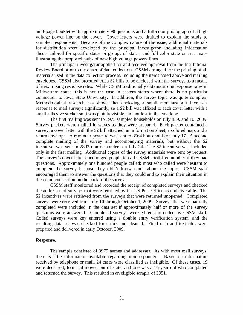
an 8-page booklet with approximately 90 questions and a full-color photograph of a high voltage power line on the cover. Cover letters were drafted to explain the study to sampled respondents. Because of the complex nature of the issue, additional materials for distribution were developed by the principal investigator, including information sheets tailored for specific states or groups of states, and full-color state or area maps illustrating the proposed paths of new high voltage powers lines.

The principal investigator applied for and received approval from the Institutional Review Board prior to the onset of data collection. CSSM arranged for the printing of all materials used in the data collection process, including the items noted above and mailing envelopes. CSSM also procured crisp $2 bills to be enclosed with the surveys as a means of maximizing response rates. While CSSM traditionally obtains strong response rates in Midwestern states, this is not the case in eastern states where there is no particular connection to Iowa State University. In addition, the survey topic was quite complex. Methodological research has shown that enclosing a small monetary gift increases response to mail surveys significantly, so a $2 bill was affixed to each cover letter with a small adhesive sticker so it was plainly visible and not lost in the envelope.

The first mailing was sent to 3975 sampled households on July 8, 9, and 10, 2009. Survey packets were mailed in waves as they were prepared. Each packet contained a survey, a cover letter with the $2 bill attached, an information sheet, a colored map, and a return envelope. A reminder postcard was sent to 3564 households on July 17. A second complete mailing of the survey and accompanying materials, but without the $2 incentive, was sent to 2892 non-responders on July 24. The $2 incentive was included only in the first mailing. Additional copies of the survey materials were sent by request. The survey’s cover letter encouraged people to call CSSM’s toll-free number if they had questions. Approximately one hundred people called; most who called were hesitant to complete the survey because they didn’t know much about the topic. CSSM staff encouraged them to answer the questions that they could and to explain their situation in the comment section on the back of the survey.

CSSM staff monitored and recorded the receipt of completed surveys and checked the addresses of surveys that were returned by the US Post Office as undeliverable. The $2 incentives were retrieved from the surveys that were returned unopened. Completed surveys were received from July 10 through October 1, 2009. Surveys that were partially completed were included in the data set if approximately half or more of the survey questions were answered. Completed surveys were edited and coded by CSSM staff. Coded surveys were key entered using a double entry verification system, and the resulting data set was checked for errors and cleaned. Final data and text files were prepared and delivered in early October, 2009. Response.

The sample consisted of 3975 names and addresses. As with most mail surveys, there is little information available regarding non-responders. Based on information received by telephone or mail, 24 cases were classified as ineligible. Of these cases, 19 were deceased, four had moved out of state, and one was a 16-year old who completed and returned the survey. This resulted in an eligible sample of 3951.

32

Throughout the course of the data collection, 146 surveys were returned by the US Post Office as undeliverable. Sometimes the selected person had moved with no forwarding address or with forwarding expired. Sometimes the address was undeliverable. Because there is no definitive ineligibility for these cases, they are presumed to be eligible for purposes of this report.

A total of 131 people either called the toll-free number to refuse or returned their survey with a note of refusal. Ten respondents were unable to complete the survey due to health reasons, such as advanced age with poor eyesight or Alzheimer’s disease. One survey was returned with “no English” written on it. There was no response at all from 50.7% of the eligible sample (50.4% of the original sample).

Completed surveys were received from 1661 respondents. Six of these removed their ID numbers, so their state or region is unknown.

Response rates for completed surveys are calculated as the percentage of surveys completed out of the eligible sample as defined above. The highest response rates were obtained in Iowa and Minnesota, both at 51.4%. They were followed by South Dakota with 45.0% and West Virginia Area 8 with 43.7%. Response rates in Maryland Area 2 and New Jersey Area 5 were 40.1% and 40.8%, respectively. The lowest response rates were in West Virginia Area 9 (36.9%), Maryland Area 3 (33.8%) and New Jersey Area 6 (31.4%). The overall response rate was 42.0%. Table 2. Sample size, number of cases by outcome, and response rates by state/region.

1 IA

2 MD

3 MD

4 MN

5 NJ

6 NJ

7 SD

8 WV

9 WV TOTAL

Sample 475 425 425 475 425 425 475 425 425 3975

Not Eligible 4 6 2 2 1 1 4 2 2 24

Eligible Sample 471 419 423 473 424 424 471 423 423 3951

Packet returned 15 12 11 11 17 19 14 25 22 146

Refused 13 16 5 19 15 9 22 10 22 131

Health barrier 1 1 1 1 3 1 1 1 10

Language barrier 0 0 0 1 0 0 0 0 0 1

No Response 200 222 264 198 218 260 222 202 222 2002

Completed 242 168 143 243 173 133 212 185 156 1655

Completed with ID removed

6

Total Completed

1661

Response Rate 51.4% 40.1% 33.8% 51.4% 40.8% 31.4% 45.0% 43.7% 36.9% 42.0%

Preliminary Results

33

The initial data were delivered to Dr. Sapp in Mid-October, 2009. The sample weights are being processed by the Center for Survey Statistics and Methodology, and thus far data analysis has limited to just a few descriptive and inferential statistics. Therefore the results presented here are preliminary in nature. Overall, respondents expressed low willingness to comply with either federal or state recommendations for building new high-voltage power lines, with respondents expressing slightly higher willingness to comply with state over federal agencies. These figures vary widely across different states, with higher scores found in the Midwestern states, lower scores within the New England states, and very low scores in West Virginia. A similar pattern of responses was found for expressions of trust in federal and state agencies to do the right thing in building additional high-voltage power lines. Approximately 53% of respondents said they were willing to pay 1% more on their utility bills to support the building of additional high-voltage power lines. Understandably, these figures drop dramatically when respondents are asked about their willingness to pay an additional 3% (38% said "yes"), 5% (24% said "yes"), 10% (10% said "yes"), or 15% (5% said "yes") more on their monthly utility bill. Causal modeling, restricted at this time to ordinary least squares regression analysis, shows that concerns about energy usage, the implementation of eminent domain by federal or state agencies, and feelings of being left out of the decision-making process are the key determinants of people's willingness to support the building of additional high-voltage power lines.