NASA Contractor Report 172199 NASA-CR-172199 19840003088

Finds: A Fault Inferring Nonlinear Detection System-User's Guide

R.E. Lancraft and A.K. Caglayan Bolt Beranek and NewmII'Ilnc. cambridge, MA 02238

Contract NAS1·18579 September 1883

NI\SI\ National Aeronautics and Space Administration

Langley Research Center Hampton, Virginia 23665

1111111111111 1111 11111 1111111111 1111111111111 NF02507

'j r.-~~ ",

L,

https://ntrs.nasa.gov/search.jsp?R=19840003088 2020-04-20T07:52:33+00:00Z

TABLE OF COIITBITS

1 • IITIODUCTIOII

2. PIOGlWI OIGAIIIZ.l.TIOIL

3. DESCRIPTIOR OF IIIPUTS

3.1 Interactive Nature of FINDS 3.2 General Input Parameter File 3.3 Sensor Input Parameter File 3.4 Filter Input Parameter File 3.5 Quick Reference to Input Files 3.6 Sample Input File Specification

4. DBSCIIPTIOR OF OUTPUTS

4.1 Summary File 4.2 Time Line File 4.3 Output File 4.4 Plot File

5. COIiCLUDIIIG COMKBRTS AIID IBCOHMEIID.l.TIOIiS

i

Page

1

3

13

14 17 24 52 55 61

65

65 71 77 81

91

n <DLi - J 1 IS le-#

· APPIIDIX 1. POST-PlOCBSBDG PlOClIAIm

A. 1 Desoription of Program: PRINTD A.2 Desoription of Program: PLOto

6. urBIIICIS

IIDII

ii

93

93 95

97

99

LIST OF FIGURES

FIG. 1. FIG. 2. FIG. 3. FIG. 4. FIG. 5. FIG. 6. FIG. 7. FIG. 8. FIG. 9. FIG. 10.

FUNCTIONAL FLOW DIAGRAM OF FINDS FAULT TOLERANT SYSTEM STRUCTURE INPUT/OUTPUT PERSPECTIVE OF FINDS FINDS INTERACTIVE SESSION FUNCTIONAL BLOCK DIAGRAM OF A GENERIC SENSOR MODEL FUNCTIONAL BLOCK DIAGRAM OF A GENERIC FAILURE MODEL INPUT FILE EXAMPLE SAMPLE SUMMARY FILE SAMPLE TIME LINE FILE

SAMPLE OUTPUT FILE

iii

5 7

11 15 26 30 62 66 76 78

This Page Intentionally Left Blank

LIST or TABLES

TABLE 1. TABLE 2. TABLE 3. TABLE 4. TABLE 5. TABLE 6.

ORDERING CONVENTIONS FOR ARRAYS SENSOR MODULE MNEMONICS SUMMARY OF NAHELIST DESCRIPTIONS SUMMARY OF .INP FILES SUMMARY OF TIME LINE CODES PLOT FILE MNEMONICS

v

9 25 56 58 73 82

This Page Intentionally Left Blank

TCV

MLS

RSDlMU

lAS

lMU

AIC

G&C

DME

RA

NF filter

LR

NL

TOF

LIST OF ABBREYIATIORS

Terminal Configured Vehicle

Microwave Landing System

Redundant Strapdown Inertial Measurement Unit

Indicated Airspeed

Inertial Measurement Unit

Aircraft

Guidance and Control

Distance Measuring Equipment

Radar Altimeter

No-Fail Filter

Likelihood Ratio

Non-Linear

Time of Failure

vii

This Page Intentionally Left Blank

Irw'Yrw'Zrw

Irw, Yrw,zrw

P,Q,R

Azm,El,Rng

NI

NUl

NYMAI

NDISTB

NFMAX

NFT

LIST OF SYMBOLS

Ale position in the runway frame (m)

Ale velocity in the runway frame (m/s)

Ale Euler angles which rotate the body axes into coincidence with the runway frame

Horizontal wind components in the runway frame

Ale acceleration in the body frame

Ale angular rates of change in the body frame

HLS azimuth, elevation, and range

Small misalignment angles

I and Y axis angular rates from two-degree-of-freedom gyro used in the RSDlMU

The total number of NF filter states (estimates)

The total number of NF filter input measurements

The maximum possible number of output measurement types

The total number of NF filter process noises

The total number of sensor types

The total number of sensors used by the NF filter

1. I1TRODUCTION

This report describes the digital computer program FINDS (Fault Inferring

Nonlinear Detection System) version 3.0 developed by Bolt, Beranek, and Newman

Inc. (BBN). 1

The objective of FINDS is to detect, isolate, and compensate for failures

in navigation-aid instruments and on-board flight control and navigation

sensors of a Terminal Configured Vehicle (TCV) aircraft in a Microwave Landing

System (MLS) environment. FINDS also provides sensor fault tolerant estimates

for the aircraft states which are used by an automatic guidance and control

system to land the aircraft along a prescribed path. FINDS monitors for

failures by evaluating all sensor outputs simultaneously and uses analytic

relationships between the various sensor outputs arising from the aircraft

point mass equations of motion. Hence, FINDS is an integrated sensor failure

detection and isolation system.

Although the specific application in this study is concerned with

aircraft sensor failures, the failure detection and isolation algorithm

developed is quite general and applicable to input, component and output

failure identification problems in discrete-time, nonlinear stochastic

systems.

To give somewhat of an historical perspective, it should be mentioned

that several programs were merged together to form the TCV environment in

which FINDS operates. The NASA-supplied program FILCOMP (formerly called

ALERT), was modified to provide the required dynamic environment as well as

lspecial thanks and acknowledgement is given to F.R. Morrell and R. Hueschen for invaluable discussions regarding NASA supplied software used in this program and documented in this report.

the MLS simulation model used. In addition, NASA also furnished a simulation

model of a developmental redundant strapdown inertial measurement unit

(RSDIMU), obtained from the program BVALT. These two programs were combined

with sensor and failure models developed by BBN, to form the simulated TCV

environment.

FINDS is written in FORTRAN-77, and is intended for operation on a

Digital Equipment Corporation's (DEC) VAX 11-780 or 11-750 super mini

computer, using the VMS operating system. The program was written in a modular

and flexible fashion to allow for ease of program verification, and future

modi fica tion.

This volume is intended to serve as a self-contained users guide to FINDS

and it's associated post-processing programs. If the reader is interested in

a more detailed understanding of the theoretical background, then review of

the contract's interim report [1], or final report [2] is recommended.

The organization of this report is as follows: Chapter 2 consists of a

brief overview of the nature of FINDS, along with a discussion on program

organization. It also contains a section which discusses the installation of

the delivered program. Chapter 3 gives a complete description of all program

inputs, as well as a typical example which clearly shows how to generate the

required input files. One feature of this chapter is a quick reference

section. The user can find both consise input specification information, as

well as cross references to very detailed descriptions. Chapter 4 reviews the

outputs available from FINDS by discussing the outputs of the example from

Chapter 3. Concluding remarks are made in Chapter 5. Appendix A consists of

descriptions of the post-processing programs which can be used in conjunction

with FINDS. Finally, a cross-reference list of all important variables and

symbols is included at the end of the report for subsequent quick reference.

2

2. PROGRAM ORGABIZATIOR

The intention of this chapter is to give the reader an overall

understanding of the operation and organization of the FINDS program. FINDS

will be examined from both an input/output point of view as well as from a

functional viewpoint. As mentioned in the introduction, FINDS is an

amalgamation of several computer programs. Since less attention will be

devoted to these NASA-supplied modules in this manual, whenever possible, the

reader will be referred to more detail'ed references. After reading this

chapter, the reader should have a sound idea of the nature of FINDS, and how

it can be used. Further details can be found in the following chapters of

this document and,in the final report [2].

The purpose of FINDS is to detect, isolate, and compensate for failures

in navigation-aid instruments and on-board flight control and navigation

sensors of a TCV aircraft in an MLS environment. FINDS also provides sensor

fault tolerant estimates for the aircraft (A/C) states, which are used by an

automatic guidance and control system to land the A/C along a prescribed path.

The user can analyze the performance of FINDS over many different conditions.

For example, each of the following conditions can be easily simulated by

FINDS:

o different flight paths

o various sensor replications (single, dual or triple redundancy)2

o different sensor parameters (normal operating noise, bias, scale factor, etc.)

2Although FINDS can simulate triple redundancy in the sensor module, the fUter/detector structure has been tested using at most dual redundancy. Therefore, the filter is constrained to use no more the dual redundancy in FINDS version 3.0

3

o different sensor configurations (i.e. ability to specity what physical sensors are used, for example to use an IMU or a RSDIMU)

o different disturbance profiles (shear, gusts, and horizontal winds)

o different failure modes, amplitudes and onset times

o effects of multiple failures or simultaneous failures

o different NF filter configurations (set of operational biases to estimate)

Chapter 3 will explain how the user can specity each of these conditions.

Provisions have been made in the program which enable the user to run the

TCV simulation with guidance and control (G&C) commands generated either from

the no-fail filter state estimates, or the "true", simulated values of these

variables. The option of running the NF filter without failure detectors is

also provided. FINDS can be run in a Monte Carlo fashion to obtain

statistical performance information, or in a comparative fashion (by using the

same noise sequence) to obtain relative performance data.

A functional block diagram of the major modules in FINDS, as well as the

overall program flow, are detailed in Figure 1. The major functional blocks

consist of the following:

o Initialization module to initialize all modules properly

o A module to compute the guidance and control commands required by the A/C simulation

o A facility to save information at the end of a simulation "tick"

o A program stopping criterion (to stop after some maximum elapsed time)

o Integration of the six-degree-of-freedom nonlinear TCV aircraft equations of motion

o A collection of realistic sensor modules (including the NASA-supplied RSDIMU and MLS), which take in the true values of measured variables

4

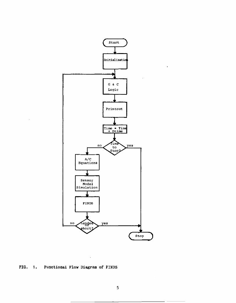
FIG. 1.

no

A/C Equations

Sensor Model

Simulation

FINDS

G & C

Logic

Printout

yes

Functional Flow Diagram of FINDS

5

from the TCV simulation and put out sensor outputs which account for misalignment, measurement noise, bias drift, normal scale factor errors and limits. This block also contains sensor failure models for simulating increased bias, hardover, null, scale factor, ramp, and increased noise type sensor malfunctions.

o FINDS fault tolerant system algorithms. This module essentially looks like a fault tolerant navigator in this diagram (it supplies reliable state estimates to the G&C module).

o Additional program stopping criterion (if the A/C has landed or if the fault tolerant navigator has issued an "abort")

The fault tolerant system module in Figure 1 represents the "heart" of

the program. Figure 2 shows this module broken down into its functional

blocks. The figure is made up of the following parts:

o a nonlinear state estimator (also called NF filter, or fault tolerant navigator) which provides sensor fault tolerant estimates for aircraft position, velocity, at ti tude, and horizontal winds along with normal operating biases for a user-selected sensor subset. This module is separated into "update" and "propagate" cycles in the diagram.

o a bank of detectors which are first-order failure level estimators for estimating bias jump failures in sensor outputs. Each detector operates over a "detection window", which is a fixed integer multiple or decision windows and synched to the start of a decision window.

o a bank or likelihood ratio (LR) computers providing the necessary LR computations for the posed multiple hypothesis testing problem. LR's are computed over a fixed length moving "decision window".

o a Bayesian decision rule which selects the most likely failure mode based on the LR computations. Decisions are made at every simulation "tick", not just at the end of decision windows.

o a sensor healing module which monitors the failed sensors (if any) to determine if they have "healed", or alternatively, if the detection logic had generated a "false alarm" by failing the sensor in the first Place. 3 The healers operate over a fixed length moving window

3The current healer module is only effective for bias, null, or hardover failures.

6

FIG. 2.

Enter

~.F. Filter (Propagate Cycle)

" Bank of

Detectors

Bank of L.R.

Computers

Decision Rules

Fault Tolerant System Structure

7

., Sensor Healing Tests

~figurati(~ Logic

~.F. Filter (update cycle)

Return

which is synched to the decision window. Healing decisions are made ~ at the end of this window.

o a reconfiguration module which performs the necessary reinitialization in the previous five blocks after the detection and isolation of a sensor failure.

More detail on each of these modules can be found in [1], and [2].

At this pOint, it will be useful to develop a set of working descriptions

which we can use throughout the manual to describe various ideas. For

instance, vectors and matrices need to have some sort of symbolic ordering in

the program, Table 1 defines several ordering conventions that were adopted

(the symbols used in the table are defined in the beginning of the manual or

in Table 2 on page 25). The table is organized by "type" and array index.

Notice that the vector length is also symbolically defined in the "type"

section. For example, if, elsewhere in this manual, reference is made to a

vector ordered by "measurement type", then we would know, from Table 1, that

the vector is nominally of length NYMAX=8 and ordered as MLS-azimuth, MLS­

elevation, MLS-range, Indicated Airspeed, IMU-phi, IMU-theta, IMU-psi, and

Radar Altimeter measurements.

Notice from Table 1, the sensor measurements are divided into two groups

(when viewed by the NF filter) called "Inputs" and "measurements". The first

group, which consists of linear accelerometer and rate gyro measurements

(either body mounted or RSDIMU supplied), are referred to as the NF filter's

input measurements or simply as input measurements. The NF filter integrates

these input measurements during the propagate cycle of the filter to obtain

the propagated state estimate. The rest of the sensor measurements are

collectively called the NF filter measurements, or simply filter measurements.

They are treated as measurements in the NF filter, and are used to compensate

the propagated state estimate during the update filter cycle.

The actual input/measurement configuration used by the NF filter is user­

definable. The following rules detail this:

8

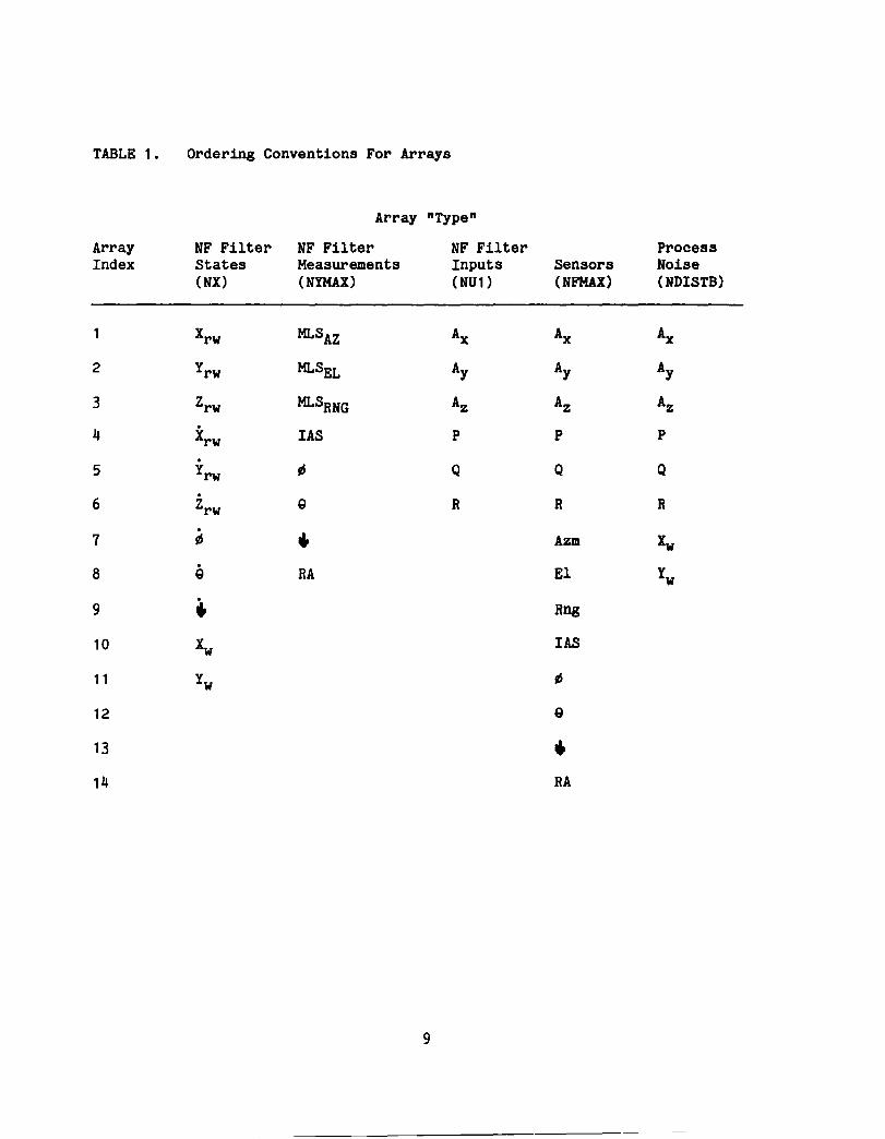
TABLE 1. Ordering Conventions For Arrays

Array "Type"

Array NF Filter NF Filter NF Filter Process Index States Measurements Inputs Sensors Noise

(NX) (NIMAX) (NUl) (NFMAX) (NDISTB)

1 Xrw MLSAZ Ax Ax Ax

2 Yrw MLSEL Ay Ay Ay

3 Zrw MLSRNG Az Az Az

4 Xrw lAS P P P

· 5 Yrw 115 Q Q Q

· 6 Zrw g R R R

· 7 115 .. Azm Xv 8 g RA El Iw

9 .. Rng

10 Iv lAS

11 Yw 115

12 g

13 .. 14 RA

9

o The number of replications of any given sensor used by the NF filter is equal to the number of replications the user has chosen to simulate (none, single, dual or triple redundancy).

o Input measurements can be obtained either from body mounted (flight control quality) sensors, or from an (navigation quality) RSDIHO.

o A single replication of input measurements are used by the NF filter. Additional replications, if simulated, are used as standby equipment.

o Attitude measurements can either be omitted from the filter, obtained from a platform IHO, or from the RSDIMU.

Figure 3 shows an input/output perspective of FINDS from the users

viewpoint. Notice that three disk files supply information to the program,

with additional input from the controlling terminal (interactive responses) or

alternatively from a batch commands file. From an overall point of view, the

three disk files suply parameters for general program control and A/C

simulation purposes, sensor/failure model simulation, and fault tolerant

system parameters, respecti vely. The files were di vided in this manner to

facilitate the Monte Carlo running of FINDS.

described in detail in Chapter 3.

Each of these files will be

On the output side, FINDS generates four disk files of output

information, with a fifth file (FINDS.LOG) created by the batch operating

system if FINDS was run via the batch processor. FINDS automatically assigns

a pre-defined file extension to each of these output files. In as much as the

four output files will be discussed in detail in Chapter 4, we will only give

a quick summary here.

o FINDS. SUM. The .SUM file basically contains a "summary" of the parameters used to generate the run. It is currently organized into a series of five tables which summarize the sensor and fault tolerant system modules.

o FINDS. TLN. The. TLN file is a "Time line" file of major discrete events which occurred during the course of the run. Whenever an "event" occurs, a coded "snapshot" of that point in the run is saved on the file. This file can later be used to obtain statistical information about FINDS failure detection performance.

10

SENSOR.INP FILTER.INP

FINDS.SUM

FINDS.PLT

FINDS. LOG

FIG. 3. Input/Output Perspective of FINDS

11

INTERACTIVE INPUTS OR, . FINDS. COM

FINDS. OUT

o FINDS. PLT • The. PLT file is an unformatted ( binary) file of time history data. The user can select the frequency and variables to be saved. He can also request that this file not be generated. This file can be post-processed to obtain tables of the data or time­history plots.

o FINDS. OUT. The .OUT file is an output file containing complete echo checks on all input file parameters as well as ASCII time history output. Options are available to either eliminate the time history outputs, or to suppress the generation of this file.

o FINDS. LOG. The .LOG file contains useful run time statistics and error messages (if any).

From the above descriptions, we see that FINDS records detailed

(continuous) time history data, discrete event information, and partial or

complete summaries of the input data used to produce the run. Furthermore,

because of the file formats choosen, uniform naming conventions, and the

separa tion of data by type ( i. e. discrete, continuous, summary, etc. ) the

information contained in each run can be post-processed to obtain ensemble as

well as temporal metrics in a convienient fashion. The collection of all runs

can almost be viewed as a distributed data base which can be saved on tape and

re-examined as new post-procesing programs become available. The only

facility missing from FINDS 3.0, which would truly make its outputs part of a

data base, is a common file which logs the names of all the runs created.

This facility is a Simple but important one to add in the future and is

mentioned here, only to draw attention to the fact that if such a facility

were available , nearly the entire post anlaysis phase of a Monte-Carlo study

would be fully automated.

12

3. DESCRIPTION OF IBPUTS

This section describes, in detail, each of the four (4) input files

required by FINDS. As you recall, from Figure 3 and the organizational

discussions of the last chapter, the four input files consist of the

following:

1. "Interactive" responses from the controlling terminal (TT:) or from a batch processor command file. We will refer to the batch command file as the FINDS. COM file.

2. "General" program control and A/C simulation inputs. This file will be referred to as the GENERAL.INP file in the ensuing discussions.

3. "Sensor" module inputs in the SENSOR.INP file.

4. "Filter" and detector module inputs. This file will be called the FILTER.INP file.

In naming each of these files we've adopted arbitrary names which are

valid VAX/VMS file specifications. Where the partial form is: "file-

name. file-extension". Although the VMS operating system allows very large file

specifications (up to 128 characters), FINDS arbitrarily limits the file name

to eight (8) characters, and the file ext. to three (3).

The .INP files are "Namelist" files; that is, they contain only Fortran

namelist style input data. If the reader is not familiar with namelist-

directed read statements, he should review pp. 5-21, 5-22, and 7-18 to 7-22 in

[7] before attempting to generate an .INP file. The basic form of a namelist

input is:

_$namelist name-Ientity=value, ••• ]$-IEND]

where _=space, and [ ••• ] represent optional arguments. Entity is a program

variable name, defined in the Fortran namelist statement. Each .INP file is

made up of several namelist-directed reads. Where all expected namelists muAi

appear within the .INP file, even if no change to the default entity values

are desired.

13

The rest of this chapter is organized as follows: Section 3.1 discusses

the interactive environment and use of the FINDS. COM file. Section

3.2-3.4 define the namelists and their associated entities for each of the

three .INP files. Section 3.2 also explains the general format of the

namelist descriptions used in Section 3.2 - 3.4. The next Section, Section

3.5, is a "quick reference" section which simply reviews, in a very

abbreviated format, all the namelist names and entity names. The last

Section, Section 3.6, contains a descriptive example to demonstrate how the

input files are generated.

3.1 Interaotive Nature ot FINDS

This section discusses FINDS' interactive environment. The program

prompts, as well as expected user responses, will all be enumerated.

The interactive environment of FINDS offers the user various convenient

features. For instance, since the program will normally be run in a Monte­

Carlo fashion, the user is faced with running the same problem over and over,

varying only the random initial conditions. By using an interactive

environment, the user can specify those quantities which are specific to a

particular run, and eliminate unnecessary duplication of the input files.

To show how the interactive environment operates and to enumerate the

user responses, a typical FINDS session is shown in Figure 4. (Note: in the

typescript, line numbers are shown for reference purposes, user responses are

in bold print, and carriage return is noted as <CR>.)

As seen from Figure 4, the interactive environment is fairly self­

explanatory. Each of the user responses are verified by FINDS before the next

question is asked. If a faulty answer is given, FINDS will force the user to

supply an acceptable one. Note that lines 3-4, 14-32, and 34-35 show how the

14

LINE No. INTERACTIONS

$ RUN FIIDS (CI> 2 SpecifY FILE NAME for Program Control Info: GBIBBAL.I1P (CI> 3 Specify FILE NAME for Sensor Hodel Info: SBlSOI.IMP (CI> 4 Can't find File:SENSOR.IMP, TRY AGAIN: SElSOI.I1P (CI> 5 SpecifY FILE NAME for Filter-Detector Info: FILTlT.I1P (CI> 6 SpecifY a GENERIC name for ALL output files 7 File group name: FIIIDSR (CI> 8 TYPE UP TO 15 LINES OF TEXT, END WITH BLANK LINE 9 STAIIDABD SEISOI COIFIOURATIOR(CR> 10 SGLTOR BIAS FAILURES -- level = 10 8~ n.o.b.(CI> 11 TIME= 15 110 150 220 253(CI> 12 TYPE= el-2(CI> 13 <CR>" 14 ANY CHANGES? : Y (CI> 15 > ?(CI> 16 ANSWER : 17 C, D ,I , R ,T , F 18 > (CR> 19 EDITOR COMMANDS ARE: 20 C Change entire title. 21 D Delete an entire line. 22 I Insert title above a line. 23 R Replace one line with another. 24 T Type current title. 25 F Finished editing. 26 NOTES : 27 LINE = 0 : Aborts command and returns to prompt level 28 Currently blank lines of text are NOT allowed 29 > R(CI> 30 LINE NO.:2(CR> 31 "SIRGLTON BIAS FAILURES -- level = 10 Sigma n.o.b.(CI> 32 > F(CR> 33 Input SEED for Random Number Generation (odd #) 0 (CR> 34 Save default variables in .PLT file? OK (CR> 35 ANSWER Y, y, N, n:R(CI>

FIG. 4. FINDS Interactive Session

15

LINE No. INTERACTIONS

36 Indicate (Y,N) which variable groups to save in the PLT file 37 No-Fail filter state est error?: Y <CR> 38 No-Fail filter state est Uncertainty?: Y <CR> 39 Bias filter state est?: Y <CR> 40 No-Fail filter inputs?: N<CR> 41 No-Fail filter Outputs?: N <CR> 42 No-Fail filter residuals?: N (CR> 43 Li, Fi, Ii for detectors?: N <CR> 44 Expanded (& filtered) residuals?: N (CR> 45 A/C latitude & longitude?: N (CR> 46 Ground track info?: Y (CR> 47 True attitudes?: Y <CR> 48 True body accel?: N (CR> 49 Airspeed?: N (CR> 50 Performance measures?: Y (CR> 51 Body P,Q,R info?: N <CR> 52 Control info?: Y (CR> 53 RSDIMU info?: N <CR> 54 Measurement ERROR histories?: N(CR> 55 FORTRAN STOP

FIG. 4. FINDS Interactive Session, concluded

program reacts to improper input and how it allows for user intervention. By

responding to line 33 with a zero input, the program chooses a "random"

initial seed, where the seed value is based on the current time of day. The

last eighteen (18) user responses, lines 36-54, define the set of variables to

be saved in the .PLT file. The implications of YIN responses to these

questions are discussed in Table 6 on page 82. If this file is not requested,

or if the answer to line 34 is Yes, then these questions will not be asked.

If all the user inputs from our interactive session (bolded text) are

saved in a BATCH. COM file, then FINDS can be run in "batch" mode, via the

VAX/VMS batch processor.

16

3.2 General Input Parameter File

This section describes the namelist directed inputs contained in the

GENERAL.INP file. This section, as well as the next two sections, contain

namelist descriptions. The general format for each namelist description will

be as follows:

Description:

co.aents:

Variables:

NlKBLLST: namelist-name

A one- or two-sentence description of the namelist.

Addi tional information, required before the variables can be specified.

A list of the variables (namelist entities), along with their definitions, range, engineering units, type, order (scalar, vector, matrix), and default value.

In order to condense the individual variable descriptions, a shorthand

convention has been adopted. The following rules define this convention:

o Once a variable has been defined, it may be used to define subsequent variables.

o The symbol "=>" should be read "is associated with" or "implies".

o The symbol"-" or "->" should be read "to", for example A(1) -> A(S).

o A variable's engineering units are always given in parenthesis, at the end of the description.

o Standard abbreviations are used for units, if space is confined.

o "Namelist style" repetition factors are used in specifying both the units and default values for vectors and matrices.

o The following coded information is contained within square brackets at the end of each description.

[A,B[=R:C], D=V] where:

17

•

•

A describes the variable type, as: R=> Real I=> Integer L=> Logical (.true. or .false.) A=> Alpha-numeric (character string)

B describes the variables structure and order, where: 4

S=> Scalar V=R=> vector with R rows M=R:C=> matrix with R rows and C columns

D describes V the default value of the variable (if no naaelist entry is made by the user), where:

D=V=> V is the default value.

For example:

Foo: A dummy variable. 0 ~ Foo .i 10.0. (2*cubits,3*furlongs), [R,V=S,D=4*3.0,10.0].

describes a real, vector valued variable of length S, called

program expects the value for Foo to be between 0.0 and 10.0.

RFooR. The

Its default

values are 3.0 cubits for the first two elements, 3.0 furlongs for the next

two elements, and 10.0 furlongs for the last element.

Desoription:

Variables:

DTIME:

FILTER:

PROGCN contains general program control quantities.

The simulation's [R,S,D=O.OS]

integration step size. (seconds),

Flag to indicate whether or not the fault tolerant navigator is to be run, where • True. => run the navigator. (unitless), [L,S,D=.False.]

4Note : by order we mean that portion of the variable which FINDS uses, and must therefore be user specified, ~ necessarily the dimensioned size of a variable.

18

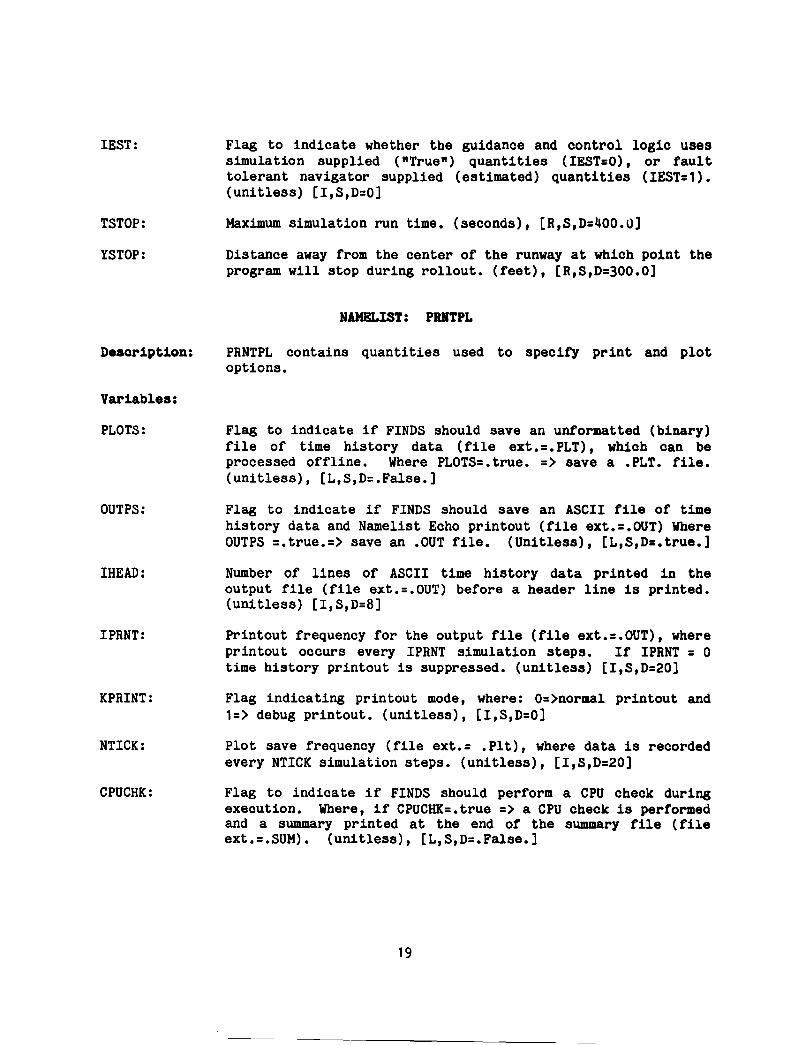
lEST:

TSTOP:

YSTOP:

Desoription:

Variables:

PLOTS:

OUTPS:

lHEAD:

IPRNT:

KPRINT:

NTICK:

CPUCHK:

Flag to indicate whether the guidance and control logic uses simulation supplied ("True") quantities (IEST=O), or fault tolerant navigator supplied (estimated) quantities (IEST=1). (unitless) [I,S,D=O]

Maximum simulation run time. (seconds), [R,S,D=400.0]

Distance away from the center of the runway at which point the program will stop during rollout. (feet), [R,S,D=300.0]

NAHBLIST: PRRTPL

PRNTPL contains quantities used to specify print and plot options.

Flag to indicate if FINDS should save an unformatted (binary) file of time history data (file ext.=.PLT), which can be processed offline. Where PLOTS=. true. => save a .PLT. file. (unitless), [L,S,D=.False.]

Flag to indicate if FINDS should save an ASCII file of time history data and Namelist Echo printout (file ext.=.OUT) Where OUTPS =.true.=> save an .OUT file. (Unitless), [L,S,D=.true.]

Number of lines of ASCII time history data printed in the output file (file ext.=.OUT) before a header line is printed. (unitless) [I,S,D=8]

Printout frequency for the output file (file ext.=.OUT), where printout occurs every lPRNT simulation steps. If IPRNT = 0 time history printout is suppressed. (unitless) [I,S,D=20]

Flag indicating printout mode, where: O=>normal printout and 1=> debug printout. (unitless), [I,S,D=O]

Plot save frequency (file ext.= .Plt), where data is recorded every NTlCK simulation steps. (unitless), [I,S,D=20]

Flag to indica te if FINDS should perform a CPU check during execution. Where, if CPUCHK=.true => a CPU check is performed and a summary printed at the end of the summary file (file ext.=.SUH). (unitless), [L,S,D=.False.]

19

Desoription:

Variables:

PITCH:

ROLL:

YAW:

CG:

RINLO:

RINLA:

AIRSPE:

HIGHT:

WEIGHT:

RHO:

THRUST:

RE:

PDEG:

QDEG:

RDEG:

Desoription:

COllll8nts:

HAHBLIST: ACSTAT

ACSTAT contains the quantities necessary to specity the aircraft's initial conditions.

Pitch angle. (degrees), [R,S,D:O]

Roll angle. (degrees), [R,S,D:O]

Yaw angle. (degrees), [R,S,D:O]

Center of gravity with respect to the mean aerodynamic chord. (feet), [R,S,D:20.0]

Longitude to CG of the A/C (degrees) [R,S,D:O]

Latitude to CG of the A/C (degrees) [R,S,D:O]

Airspeed (knots) [R,S,D:O]

Vertical height measured to the CG of the A/C (feet), [R,S,D:O]

Total initial weight of the A/C (pounds) [R,S,D:90000.0]

Atmospheric density (slugs/ft3) [R,S,D:0.002308119]

Thrust (pounds) [R,S,D:13900.0]

Radius of the earth (feet), [R,S,D:20,925,705.0]

Pitch rate (degrees/second) [R,S,D:O]

Roll rate (degrees/second) [R,S,D:O]

Yaw rate (degrees/second) [R,S,D:O]

HAHBLIST: WIBDAT

WINDAT contains quantities necessary to define the wind models simulated.

See [11] for a discussion of wind models.

20

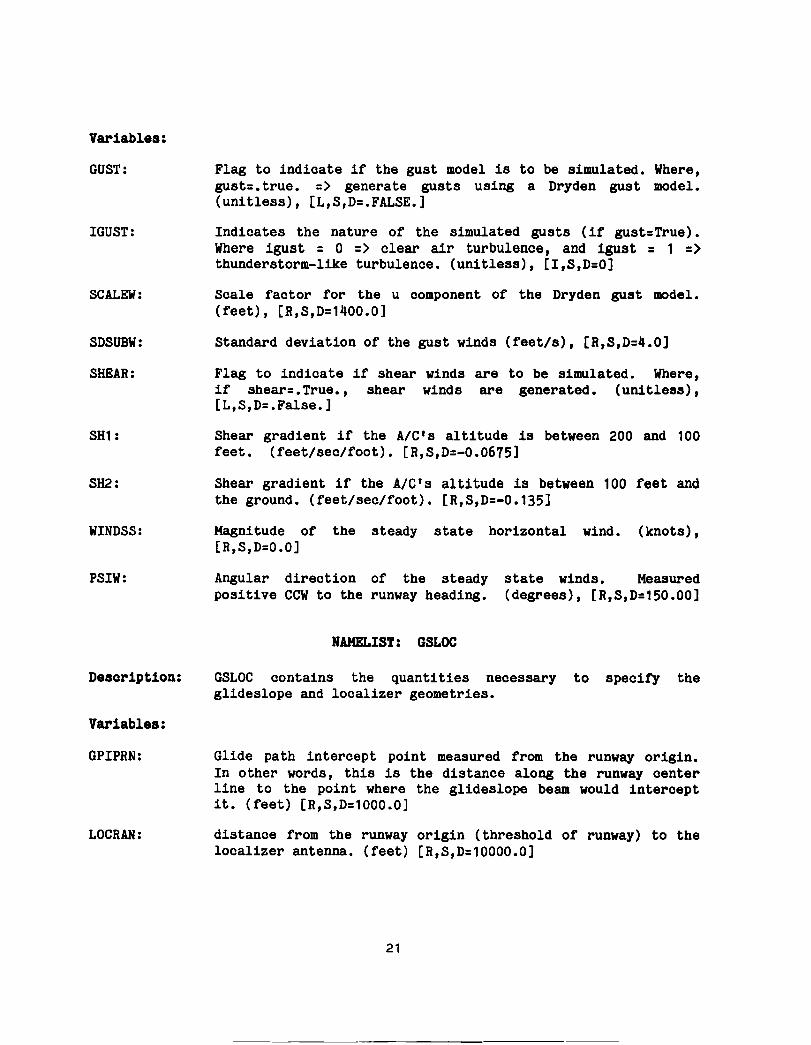
Variables:

GUST:

IGUST:

SCALEW:

SDSUBW:

SHEAR:

SH1:

SH2:

WINDSS:

PSIW:

Description:

Variables:

GPIPRN:

LOCRAN:

Flag to indicate if the gust model is to be simulated. Where, gust=.true. => generate gusts using a Dryden gust model. (unitless), [L,S,D=.FALSE.]

Indicates the nature of the simulated gusts (if gust=True). Where igust = a => clear air turbulence, and igust = 1 => thunderstorm-like turbulence. (unitless), [I,S,D=O]

Scale factor for the u component of the Dryden gust model. (feet), [R,S,D=1400.0]

Standard deviation of the gust winds (feet/s), [R,S,D=4.0]

Flag to indicate if shear winds are to be simulated. Where, if shear=.True., shear winds are generated. (unitless), [L,S,D=.False.]

Shear gradient if the AlC's altitude is between 200 and 100 feet. (feet/sec/foot). [R,S,D=-0.0675]

Shear gradient if the A/C's altitude is between 100 feet and the ground. (feet/sec/foot). [R,S,D=-0.135]

Magnitude of the steady state horizontal wind. (knots), [R,S,D=O.O]

Angular direction of the steady positive CCW to the runway heading.

RAMELIST: GSLOC

state winds. Measured (degrees), [R,S,D=150.00]

GSLOC contains the quantities necessary to specify the glides lope and localizer geometries.

Glide path intercept point measured from the runway origin. In other words, this is the distance along the runway center line to the point where the glideslope beam would intercept it. (feet) [R,S,D=1000.0]

distance from the runway origin (threshold of runway) to the localizer antenna. (feet) [R,S,D=10000.0]

21

PSIR:

THETAG:

Desoription:

CoameDtS:

Runway heading measured positive CCW to true north. (degrees) [R,S,D=O.O]

Glide slope angle measured (positive) from the runway to the glideslope beam. (degrees) [R,S,D=3.0]

HAHBLISt: StARTER

STARTER contains the quantities necessary to specify the desired nominal route the aircraft is to follow.

Nominal route construction is also referred to as waypoint path construction. A waypoint is a point in space which marks a change in the nominal route. In this version of the program, waypoints are only used to mark three conditions:

1. The start of the route. This is required to be the first waypoint. The first leg of the route is further required to be a straight line segment.

2. Changes in AIC heading.

3. The 3-D touchdown pOint, that is, the desired pOint on the runway at touchdown. This waypoint is required to be the last waypoint specified.

How can the user change the nominal altitude or velocity profile? These quantities can be specified at waypoints and a path is determined based on them, ~ they must be assooiated with a change in heading in this version of the program. That is, one cannot institute a change from level flight to one of constant sink rate, unless it also involves heading change. Therefore, one must plan the route carefully, based on the above constraints.

The following preliminary steps are normally required before use of STARTER

1. Draw the desired ground track in the runway (rw) plane, noting the (x,y,z) coordinates of path intercept pOints, along with glideslope and velocity changes.

2. Obtain the latitude, longitude and mean sea level (MSL) to the origin of rw frame.

3. Transform all points in the rw frame to appropriate latitude, longitude and altitude

22

variables:

NW:

WLO:

WLA:

SLO:

SLA:

SHZ:

HG:

VGD:

RT:

NEWPTH:

KPATH:

Additional details on waypoint path construction can be found in [3]-[5].

The total number of waypoints to be specified, where: 2 < NW < 10. (unitless), [I,S,D=none]

Longitude of each waypoint. (degrees), [R,V=NW,D=none]

Latitude of each waypoint. (degrees), [R,V=NW,D=none]

Longitude of Vortac (not used in FINDS 3.0) and HLS frame origins respectively. (degrees), [R,V=2,D=none]

Latitude of Vortac (not used in FINDS 3.0) and HLS frame origins respectively (degrees), [R,V=2,D=none]

Mean sea level altitude of Vortac (not used in FINDS 3.0) and HLS frame origins respectively. (feet), [R,V=2,D=none]

Mean sea level altitude of each waypoint. [R,V=NW,D=none]

(feet) ,

Desired airspeed at each waypoint. NOTE: .IlQt. ground speed. (knots), [R,V=NW,D=none]

Radius of turn at each intermediate waypoint. There are no "RT" items for the first and last waypoints. (feet) , [R,V=NW-2,D=none]

Flag to indicate waypoint modification at transition to HLS coverage, where:

0=> continue with original path after HLS transition (unitless), [I,S,D=O]

1=> introduce a new waypoint at HLS transition and construct a new path to next waypoint

Flag to indicate the type of waypoint path construction used, where:

0=> zero cross-track error method. This attempts to null out the cross track error at the expense of ground track angle errors. Therefore, the Ale is forced to follow the nominal ground track. This method normally exhibits the most oscillatory behavior.

23

IC:

TANLIH:

SNDP:

1=> Tangent path update method. This method attempts to construct a path from the current A/C position to a tangent point on the next waypoint turn circle. This method is smoother than the previous method in general, since it allows for some deviation from nominal. One characteristic of the method is that the total turn angle can be different than the nominal turn angle.

2=> Continued track method. This method extrapolates the current segment and determines its intersection with the next (straight line) segment. It then simply redefines the next waypoint to be the computed intersection point. This method is characteristically the smoothest. (unitless), [I,S,D=none]

Flags which indicate whether the waypoint longitudes and latitudes (WLO & WLA) are to be interpreted as the centers of turns or as the intercept point of the current path with the next path, where: 0 => corner point; 1 => center of turn. (unitless), [I,V=NW-2,D=none]

If KPATH=1, and the distance to the next turn is less than TANLIH at the point of HLS interception, then the program will default to KPATH=O or KPATH=1. [R,S,D=3000.0]

Indicator of the sign of the heading change to each intermediate waypoint path segment. For example, SNDP = -1.0 would indicate that heading will be decreasing (left turn) while turning onto the next path segment. (unitless), [R,V=NW-2,D=none]

3.3 SeDSor Input Parameter File

This section describes the namelist directed inputs contained in the

SENSOR.INP file. Each namelist defines the parameters necessary to simulate

the normal operation or various failure modes of a given sensor.

Since, by design, there is considerable structure and similarity in the

sensor modules, the following table of mnemonics should aid the reader in

better understanding the individual variables to be defined.

24

TABLE 2. Sensor Module Mnemonics

Namelist name prefixes:

MP: FP: FDI:

Model Parameters Failure model Parameters Failure Detection and Isolation

Sensor module identifiers, variable suffixes:

RA: AS: RG: LA: AG: RA: ML or MLS: GR: AR:

Radar Altimeter Indicated Air Speed body mounted Rate Gyro body mounted Linear Accelerometers inertial measurement unit Attitude Gyro Radar Altimeter Microwave Landing System rate Gyros contained in the RSDIMU linear Accelerometers contained in the RSDIMU

Variable name prefixes:

ID: IREP: DT: SDN: SDMN: SDB: SDSF: SLIM: SDTM:

FIN: FIB: FR: FSF: TF:

Initialization iDentifier Integer REPlication factor sample time (dt) Standard Deviation of the white Noise Standard Deviation of the Multiplicative Noise Standard Deviation of the normal operating Biases Standard Deviations of the Scale Factor biases Stop LIMits Standard Deviations of the misalignment Transformation Matrix Failure level for Increased Noise failures Failure level for Increased Bias failures Failure level for Ramp failures Failure levels for Scale Factor failures Time of Failure matrix (scheduled failures)

25

•

Using the l1Ilemonics def ined in Table 2 we will def ine a generic sensor

model, and a generic failure model. The generic sensor model will define the

nomal operation of all but two of the sinulated sensors. '!be two sensor

IOOdules which do not adhere to this model are the MLS and the RSDIKJ sensors.

'!bese two were both NASA-supplied and will therefore be explained separately

and briefly. The failure roodel to be defined is used by sll. the sensor

roodules. Both generic models define features which can be sinulated; however,

not all the sensors utilize the full set of features. Variables defined in

the individual nanelist description will make it clear what subset of the

generic models are actually being simulated for any given sensor.

mltiplicati ~ normal .. Misalignnent --.. or ---. operating .. ... additive r noise bias

.

scale --.. factor ... limiter ... x ... error - .. m

'!he generiC sensor model is shown in a functional block diagram in Figure

5 where we def ine:

26

xt = true value of the quantity to be sensed (veotor variable in general).

Xm = measured value of Xt.

Misalignments are produced via:

Xm = TM - xt

where TM = misalignment transformation matrix of the form (assuming xt is third order):

1

TM =

where each of the small misalignment angles are chosen as:

9 = SDTM if ID=l (i.e., deterministic initialization) or; 9 = SDTM-sample, if ID=2 (i.e., random initialization)

(1)

(2)

"Sample" is a sample from a normal, zero mean unit variance random number

generator.

Multiplicative or additive noises are added to Xm by:

Xm = (l+MNOISE)-Xm or, Xm = Xm + ANOISE

27

(3)

(4)

where MNOISE and ANOISE represent multiplicative and additive noise terms chosen as:

MNOISE = SDMN, and ANOISE = SDN if ID=l or, MNOISE = SDMN*sample, and ANOISE = SDN*sample if ID=2.

Normal operating biases are then added via:

Xm = Xm + BIAS

where BIAS is chosen as:

BIAS = SDB or, BIAS = SDB*sample

if ID=l,

if ID=2.

Scale factor errors are added as:

Xm = (l+SF)Xm

where SF is the scale factor error term chosen as:

SF = .Ol*SDSF or, SF = .Ol*SDSF*sample

if ID=l,

if ID=2.

28

( 5)

(6)

The resulting signal is then processed by either a two-sided symmetric

limiter:

Xm= -SLIM if Xm < -SLIM Xm= Xm if -SLIM ~ Xm ~ SLIM (1) Xm= SLIM if XM > SLIM

or a two-sided anti-symmetric limiter:

Xm = SLIM( 1) if Xm < SLIM(1) Xm = Xm if SLIM(1) ~ Xm ~ SLIM(2) (8) Xm = SLIM(2) if Xm > SLIM(2).

Equations (1)-(8) completely define the general form of the sensor modules.

An important feature of the sensor module defined above, is the parameter

"ID". This parameter allows the user to set the sensor's model paramters in a

random (appropriate for most is instances) or deterministic fashion (useful

for debugging or forcing specific settings).

The generic failure model, mentioned earlier is shown functionally in

Figure 6. Notice that increased noise, bias, scale factor and ramp failures

are processed before the sensor model, while hardover and null failures are

added after the measurement is Simulated. The reason for thiS, as we will

see, is because the firs t four failure types actually modify the sensor's

model parameters used in the simulation.

In order to determine if it is time to simUlate a failure, TF is

monitored by the program at every simulation step. TF determines when , how

and what specific sensor will fail. It therefore serves as a mapping between

sensor type/replication, failure mode and time of failure. This mechanism is

easiest to see by way o~ example. Let us assume we would like to simulate a

bias failure in the second replication of the radar altimeter measurement. We

would see by reading the description of namelist FPRA found on page 36 that

TFRA is a matrix arranged (symbolically) as:

29

FIG. 6.

no

no

Increased Scale Fact

Failure

Ramp Failure

Sensor Model

Simulation

no

Return

Functional Block Diagram of a Generic Failure Model

30

Hardover Failure

Null Failure

NOISE BIAS S.F. HARDOVER NULL

Tfail

Where the elements of TF are desired failure t1aes. The syabol It. It

signifies the default (program supplied) value, whioh is greater than the

desired simulation stopping time. Therefore, if no speoitioation is made by

the user in TF, then no failures will be simulated. To s1aulate a tailure,

the desired failure time (Tfail) should be set into the element ot TFRA, whose

row index oorresponds to the desired failure type/replioation, and whose

oolumn index oorresponds to the desired failure mode.

TFRA(2,2) = Tfail would aooomplish this.

In our example,

The aotual time of failure, used by the program, is determined by:

TF = TF if ID=l ( 9) or TF = ITFI + INTERVAL.USAMPLE if ID = 2, or TF < 0.0

Where SAMPLE is a random sample from a uniform [0,1] distribution, and

INTERVAL is ourrently 6 seoonds. Therefore, if random 1n1tialization is

ohoosen (ID=2) the time of failure will be between TF and TF + 6 seoonds.

Onoe the program has determined that it is time tor a given tailure to

ooour (time L TF(i,j» one of the following operations are pertormed:

o Inoreased noise failure:

31

HNOISE = SDHN.FIN (10)

if multiplicative noise is being simulated or,

ANOISE = SDN.FIN ( 11)

if additive noise is simulated in the sensor model.

o Increased Bias failure:

BIAS = SDB.FIB ( 12)

o Increased Scale factor failure:

SF = SDSF.FSF ( 13)

o Ramp failure:

BIASk+1 = BIASk + DT·FR (14)

where k and k+1 refer to the time scale.

o Hardover failure:

32

Xm = SLIM

Xm = -SLIM

o Null failure

Xm = 0.0

if Xm L 0

if Xm < 0

( 15)

(16)

Equations 9-17 completely describe the generic failure model employed.

The MLS simulation module, developed by NASA, is described in detail in

[3], and [5]. The MLS model is sufficiently complex that it is beyond the

scope of this report; however, in order to give the reader some notion of the

simulation model, a brief description is included.

The MLS ground system basically consists of an azimuth antenna and

elevation antenna. The azimuth antenna is usually located on the runway

centerline beyond the stop end, and the elevation antenna is located on either

side of the runway in the vicinity of the glidepath intercept point (GPIP).

The azimuth beam sweeps "TO" and "FRO", up to +600 about the runway centerline

and the elevation beam sweeps up and down similarly between 0 and 200 of

coverage. The MLS also consists of a DME antenna to give precision range

information which is colocated with the azimuth antenna.

The airborne equipment consists of a receiving antenna, an angle receiver

for the elevation and azimuth signal detection, and a DME receiver for the

range signal. The receiver measurements are digital in nature (- 13 Hz for

Azimuth, 40 Hz for elevation and 30 Hz for range).

The MLS simulation model computes the azimuth, elevation and range

signals based on the aircraft's position and velocity in runway rectangular

33

coordinates. The model also determines whether the AIC is within coverage of

the ground antenna.

The HLS has a time multiplex format in which the antenna scans are not

separated at equal time intervals. This time shift is referred to as

"jitter". The model computes time increments which represent the signal

decoded time relative to current simulation time. Given these time

increments, the aircraft's position is determined for the time when the

receiver decoded the signal. This is done only for the azimuth and elevation

signals. From the position corrected due to time shift, the model computes

the azimuth, elevation and range measurement. Time correlated nOise,

generated by passing Gaussian random numbers with zero mean and standard

deviation one through a linear filter, is added to the various signals along

with a constant bias. These parameters, as well as many of those mentioned in

the previous paragraphs, can be specified by the user at run time.

The model generates frame flags and outlier data (spurious spikes) by use

of a random number generator with uniform distribution. These same frame

flags are also set when the aircraft is out of a given signal coverage.

The RSDlMU is an experimental redundant strapdown inertial measurement

unit developed by NASA Langley Research Center. The unit consists of four

two-degree-of-freedom (TDOF) tuned-rotor gyros, and four TDOF pendulous

accelerometers in a skewed and separable semi-octahedron array. When coupled

to flight computers, the RSDIMU becomes a self-contained, flightworthy

inertial navigation system providing medium range accuracy with fail-opt

fail/op capability as described in [6], [10] and [8].

The RSDlMU sends to the external flight computers gyro and accelerometer

data resolved along the ideal instrument fixed coordinate reference set. Spin

axis velocity and earth-rate terms provided to the lMU from the flight control

computers are used for calibration and compensation.

34

The RSDlMU has its own local failure detection and isolation scheme

(parity checks, edge vector test, or generalized likelihood ratio test) which

can survive two gyro and two accelerometer failures [6], as well as redundancy

management logic.

Desoription:

Variables:

IDRA:

IREPRA:

DTRA:

SDNRA:

SDBRA:

SLIMRA:

HAHELIST: HPH!

MPRA specifies all model parameters necessary for simulation of the radar altimeter sensors.

Flag enabling deterministic or random parameter initialization. Where IDRA=2 normal operating biases are randomly selected, and IDRA=1 & TOF deterministic initialization is performed. (unitless), [I,S,D=2].

The desired number of replications to be simulated. Currently, O~IREPRA~. (unitless), [I,S,D=1].

The desired sample time for radar altimeter measurements. Note: This feature is currently disabled in FINDS version 3.0. (seconds), [R,S,D=DTlHE].

Standard deviations of the additive noises. One value for each replication. (meters), [R,V=IREPRA,D=3.0.3048].

Standard deviations of a zero mean Gaussian distribution from which the normal operating biases are chosen, if IDRA=2. Otherwise, if IDRA=1, SDBRA represents the actual normal operating bias levels. One value for each replication. (meters), [R,V=IREPRA,D=3.0.3048].

Symmetric stop limits on the radar altimeter signal generated. Note: this feature is currently disabled in FINDS version 3.0. However, SLIMRA is used as the hardover failure level. (See NAHELIST FPRA). (meters), [R,S;D=10000.0].

35

Desoription:

Variables:

FINRA:

FIBRA:

FRRA:

TFRA:

Desoription:

Variables:

IDAS:

NAMELIST: FPRA

To specify all the desired failure modes and onset times for the radar altimeter sensors. Currently allowed failure modes include: increased nOise, increased bias, hardover, null and ramp.

Failure level for increased noise type failures. Specified as the number of standard deviations of the normal (1.) noise level of the first replication (SDNRA( 1». Note if SDNRA(1)=0.0 (i.e. noiseless) then FINRA will be interpreted as the actual failure level. (unitless, or meters), [R,S,D=10.0]

Failure level for increased bias type failures. Specified by number of standard directions of the (1.) normal operating bias level of the first replication (SDBRA( 1». Note if SDBRA(1) = 0.0 (i.e., no bias) then FIBRA will be interpreted as the actual failure level. (unitless, or meters), [R,S,D=S.O].

Failure level for ramp failures. Specified by the slope of the ramp failure. (meters/sec) [R,S,D=O.O].

Time of failure matrix used to select the sensor and failure mode to be simulated. Where the rows of TFRA represent the replication number, and the columns represent the failure modes ordered as: increased nOise, bias, hardover, null, and ramp failures respectively. (seconds), [R,H::IREPRA:5, D=1S*(TSTOP+DTlME)]

NAMELIST: MPAS

HPAS specifies all model parameters necessary for simulation of the airspeed sensors.

Flag enabling deterministic or random parameter initialization. If IDAS=2 normal operating biases are randomly selected. If IDAS=1 deterministic initialization is performed. (unitless), [I,S,D=2].

36

IREPAS:

DTAS:

SDMNAS:

SDBAS:

SLlKAS:

Desoription:

Variables:

FINAS:

FIBAS:

FRAS:

The desired number of replications to be simulated. Currently, O~REPAS~. (unitless), [I,S,D=l].

The desired sample time for airspeed measurements. Note: This feature is currently disabled in FINDS version 3.0. (seconds), [R,S,D=DTIME].

Standard deviations of the multiplicative noises. One value for each replication. (percent), [R,V=IREPAS,D=3.2.0].

Standard deviations of a zero mean Gaussian distribution from which the normal operating biases are chosen, if IDAS=2. Otherwise, if IDAS=l, SDBAS represents the agtual normal operating bias levels. One value for each replication. (meters/s), [R,V=IREPAS,D=3.1.0].

Asvmmetric stop limits on the airspeed signal generated. Note: SLIMAS is used as the hardover failure level. (See NAHELIST FPAS). (meters/s), [R,S;D=400.0,100.0].

HAHBLIST: FPAS

To specify all the desired failure modes and onset times for the airspeed sensors. Currently allowed failure modes include: increased noise, increased bias, hardover, null and ramp.

Failure level for increased multioligatiye noise type failures. Specified as the number of standard deviations of the normal (1.) noise level of the first replication (SDNAS(l». Note if SDNAS(l)=O.O (i.e. noiseless) then FINAS will be interpreted as the agtual failure level. (un1tless, or percent), [R,S,D=10.0]

Failure level for increased bias type failures. Specified by number of standard deviations of the (1.) normal operating bias level of the first replication (SDBAS( 1». Hote if SDBAS(l) = 0.0 (i.e., no bias) then FIBAS will be interpreted as the agtual failure level. (unitless, or meters/s), [R,S,D=5.0].

Failure level for ramp failures. Specified by the slope of the ramp failure. (meters/s/s) [R,S,D=O.O].

37

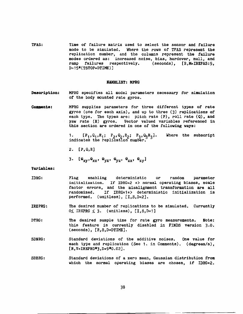
TFAS:

Desoription:

CODIIIents:

Variables:

IDRG:

IREPRG:

DTRG:

SDNRG:

SDBRG:

Time of failure matrix used to select the sensor and failure mode to be simulated. Where the rows of TFAS represent the replication number, and the columns represent the failure modes ordered as: increased noise, bias, hardover, null, and ramp failures respectively. (seconds) , [R, M=IREPAS: 5, D=15*(TSTOP+DTIME)]

NAMELIST: KPRG

MPRG specifies all model parameters necessary for simulation of the body mounted rate gyros.

MPRG supplies parameters for three different types of rate gyros (one for each axis), and up to three (3) replications of each type. The types are: pitch rate (P), roll rate (Q), and yaw rate (R) gyros. vector valued variables referenced in this section are ordered in one of the following ways:

Where the subscript

2. [P,Q,R]

Flag enabling deterministic or random parameter initialization. If IDRG=2 => normal operating biases, scale factor errors, and the misalignment transformation are all randomized. If IDRG=1=> deterministic initialization is performed. (unitless), [I,S,D=2].

The desired number of replications to be simulated. Currently O~ IREPRG ~ 3. (unitless), [I,S,D=1]

The desired sample time for rate gyro measurements. Note: this feature is currently disabled in FINDS version 3.0. (seconds), [R,S,D=DTIME].

Standard deviations of the additive noises. One value for each type and replication (See 1. in Comments). (degrees/s), [R,V=IREPRG*3,D=g*0.02].

Standard deviations of a zero mean, Gaussian distribution from which the normal operating biases are chosen, if IDRG=2.

38

SDSFRG:

SLIHRG:

SDTHRG:

Desoription:

Variables:

FINRG:

FIBRG:

Otherwise, if IDRG=1, SDBRG represents the actual normal operating bias levels. One value for eaoh type and replication (see 3.3. in COllll8nts). (degrees/s), [R,V=IREPRG.3, D=9.0.278E-4].

Standard deviations of a zero mean, Gaussian distribution from which the scale factor errors are chosen, if IDRG=2. Otherwise, if IDRG=1, SDBFRG represents the actual scale factor errors. One value for each type and replication (See 1. in Comments). (percent), [R,V=IREPRG.3,D=0.01].

Symmetric stop limits on the rate gyro each gyro type. (See 2. in Comments). the hardover failure level (See (degrees/s), [R,V=3, D=100.0].

signals. One value for SLIHRG is also used as

also NAMELIST FPRG) •

Standard deviations of a zero mean, Gaussian distribution from which the non-unity elements of the misalignment transformation matrix are chosen, if IDRG=2. Otherwise, if IDRG= 1 , SDTHRG represents the actual elements in the misalignment transformation matrix (See 3. in Comments). (degrees), [R,V=6, D=O.4].

IlAMBLIST: FPRG

FPRG specifies all the desired failure modes and onset times for the rate gyro sensors. Currently allowed failure modes include: increased noise, increased bias, increased scale factor, hardover, null, and ramp.

Failure level for increased noise type failures. Specified as the number of standard deviations of the normal (1.) noise level of the first replication (SDNRG( 1 )-)SDNRG(3». Note: if SDNRG(i)=O.O (i.e. noiseless) then FINRG(i) will be interpreted as the actual failure level. One value for each gyro type. (unitless, or degrees/s), [R,V=3, D=3.10.0].

Failure level for increased bias type failures. Specified as the number of standard deviations of the (1.) normal operating bias level (SDBRG(1)-)SDBRG(3». Note: if SDBRG(i)=O.O (i.e. no bias) then FIBRG(i) will be interpreted as the actual failure level. One value for each gyro type. (unitless, or degrees/s), [R,V=3, D=3.100.0].

39

FRRG:

FSFRG:

TFRG:

Desoript.ion:

COIlll8Dt.s:

Variables:

IDLA:

Failure level for ramp failures. Specified by t.he slope of the ramp failure. One value for each gyro type. (degrees/s/s), [R,V=3, D=O.O].

Failure level for scale factor failures. Specified as the number of standard deviations of the normal (1.) soale faotor error level (SDSFRG( 1 )->SDSFRG(3» • Note: if SDSFRG( i) =0.0 (i.e. no scale factor errors) then FSFRG(i) will be interpreted as the aotual failure level. One value for each gyro type. (unitless, or degrees/s), [R,V=3, D=100.0].

Time of failure matrix used to select the sensor and failure mode to be simulated. Where the rows of TFRG correspond to the sensor type/replication number and the columns represent the failure modes. The rows are ordered as per item 1. on page 38, and the columns are ordered: increased nOise, bias, scale factor, hardover, null, and ramp failures. (seconds), [R,M=IREPRG*3:5, D=54*(TSTOP+DTlME)].

NAMBLIST: MPLA

MPLA specifies all model parameters necessary for simulation of the body mounted linear accelerometers.

MPLA supplies parameters for three different types of linear accelerometers (one for each axis), and up to three (3) replications of each type. The types are: forward (Ax), lateral (Ay), and vertical (Az) accelerometers. Vector valued variables referenoed in this seotion are ordered in one of the following ways:

1. [AX1 , AY1 ,Az1; Ax2, AY2,Az2; Ax3 ,Ay3,AZ3]. subscript indicates the replication number.

2. [Ax,Ay,Az]

Where the

Flag enabling deterministic or random parameter initialization. If IOLA=2 => normal operating biases, scale factor errors, misalignment transformation angles and TOF are all randomized. If IOLA=1=) deterministic initialization is performed. (unitless), [I,S,0=2].

40

IREPLA:

DTLA:

SDNLA:

SDBLA:

SDSFLA:

SLIHLA:

SDTHLA:

Desoription:

Variables:

FINLA:

The desired number of replications to be simulated. Currently O~ IREPLA ~ 3. (un1tless), [I,S,D=l]

The desired sample time for accelerometer measurements. Note: this feature is currently disabled in FINDS version 3.0. (seconds), [R,S,D=DTIHE].

Standard deviations of the additive noises. One value for each type and replication (See 1. in Comments). (g' s) , [R,V=IREPLA·3,D=9·0.01].

Standard deviations of a zero mean, Gaussian distribution from which the normal operating biases are chosen, if IDLA=2. Otherwise, if IDLA=l, SDBLA represents the actual normal operating bias levels. One value for each type and replication (see 1 in Comments). (g' s) , [R, V=IREPLA.3, D=9·0.01].

Standard deviations of a zero mean, Gaussian distribution from which the scale factor errors are chosen, if IDLA=2. Otherwise, if IDLA=l, SDBFLA represents the actual scale factor errors. One value for each type and replication (See 1. in Comments). (percent), [R,V=IREPLA.3,D=O.25].

Symmetric stop limits on the rate gyro signals. One value for each gyro type. (See 2. in Comments). SLIHLA is also used as the hardover failure level (See also NAHELIST FPLA). (g's), [R,V=3, D=2·0.5,2.0].

Standard deviations of a zero mean, Gaussian distribution from which the non-unity elements of the misalignment transformation matrix are chosen, if IDLA=2. Otherwise, if IDLA=l, SDTMLA represents the actual elements in the misalignment transformation matrix (See 3. in Comments). (degrees), [R,V=6, D=O.36].

HAMELIST: FPLA

FPLA specifies all the desired failure modes and onset times for the linear accelerometer sensors. Currently allowed failure modes include: increased nOise, increased bias, increased scale factor, hardover, null, and ramp.

Failure level for increased noise type failures. Specified as

41

FIBLA:

FRLA:

FSFLA:

TFLA:

Desoription:

eo-&nts:

the number of standard deviations of the normal (1.) noise level of the first replication (SDNLA{ 1)-)SDNLA{3». Note: if SDNLA(i)=O.O (i.e. noiseless) then FINLA(i) will be interpreted as the actual failure level. One value for each accelerometer type. (unitless, or gls), [R,V=3, D=3-10.0].

Failure level for increased bias type failures. Specified as the number of standard deviations of the (1.) normal operating bias level (SDBLA(1)-)SDBLA{3». Note: if SDBLA(i)=O.O (i.e. no bias) then FIBLA{i) will be interpreted as the actual failure level. One value for each accelerometer type. (unitless, or g's), [R,V=3, D=3-10.0].

Failure level for ramp failures. Specified by the slope of the ramp failure. One value for each accelerometer type. (giS/S), [R,V=3, D=O.O].

Failure level for scale factor failures. Specified as the number of standard deviations of the normal (1.) scale factor error level (SDSFLA{1)-)SDSFLA{3». Note: if SDSFLA{i)=O.O (i.e. no scale factor errors) then FSFLA{i) will be interpreted as the actual failure level. One value for each accelerometer type. (unitless, or gls), [R,V=3, D=100.0].

Time of failure matrix used to select the sensor and failure mode to be simulated. Where the rows of TFLA represent the sensor type/replication number and the columns represent the failure modes. The rows are ordered as per 1. on page 40, and the columns are ordered: increased noise, bias, scale factor, hardover, null, and ramp failures. (seconds), [R,M=IREPLA-3:5, D=54-(TSTOP+DTlME)].

NAMELIST: HPAG

MPAG specifies all model parameters necessary for simulation of the body mounted attitude gyros.

MPAG supplies parameters for three different types of attitude gyros (one for each axiS), and up to three (3) replications of each type. The types are: pitch (~), roll (9), and yaw (t) attitude gyros. Vector valued variables referenced in this section are ordered in one of the following ways:

Where the subscript

42

Variables:

IDAG:

IREPAG:

DTAG:

SDNAG:

SDBAG:

SLIMAG:

Desoription:

Variables:

FINAG:

Flag enabling deterministic or random parameter initialization. If IDAG=2 => normal operating biases are randomized. If IDAG=1=> deterministic initialization is performed. (unitless), [I,S,D=2].

The desired number of replications to be simulated. Currently O~ IREPAG ~ 3. (unitless), [I,S,D=1]

The desired sample time for attitude gyro measurements. Note: this feature is currently disabled in FINDS version 3.0. (seconds), [R,S,D=DTIME].

Standard deviations of the additive noises. One value for each type and replication (See 1. in Comments). (degrees), [R,V=IREPAG*3,D=9*0.23].

Standard deviations of a zero mean, Gaussian distribution from which the normal operating biases are chosen, if IDAG=2. Otherwise, if IDAG=1, SDBAG represents the actual normal operating bias levels. One value for each type and replication (See 1. in Comments). (degrees), [R,V=IREPAG*3, D=9*0.1].

Symmetric stop limits on the attitude gyro signals. One value for each gyro type. (See 2. in Comments). SLIMAG is also used as the hardover failure level (See also NAMELIST FPAG). (degrees), [R,V=3, D=2*80.0,600.0].

NAHELIST: FPAG

FPAG specifies all the desired failure modes and onset times for the attitude gyro sensors. Currently allowed failure modes include: increased noise, increased bias, hardover, null, and ramp.

Failure level for increased noise type failures. Specified as the number of standard dev ia tions of the normal (1.) noise level of the first replication (SDNAG( 1 )->SDNAG(3». Note: if SDNAG(i)=O.O (i.e. noiseless) then FINAG(i) will be

43

FlBAG:

FRAG:

TFAG:

Desoription:

Co_ents:

interpreted as the actual failure level. One value for each gyro type. (unitless, or degrees), [R,V=3, D=3.10.0].

Failure level for increased bias type failures. Specified as the number of standard deviations of the (1.) normal operating bias level (SDBAG(1)->SDBAG(3». Note: if SDBAG{i)=O.O (i.e. no bias) then FlBAG{i) will be interpreted as the actual failure level. One value for each gyro type. (unitless, or degrees), [R,V=3, D=3.5.0].

Failure level for ramp failures. Specified by the slope of the ramp failure. One value for each gyro type. (degrees/s), [R,V=3, D=O.O].

Time of failure matrix used to select the sensor and failure mode to be simulated. Where the rows of TFAG represent the sensor type/replication number and the columns represent the failure modes. The rows are ordered as per 1 on page 42 and the columns are ordered: increased noise, bias, scale factor, hardover, null, and ramp failures. ( seconds) , [R,M=lREPAG.3:5, D=45·(TSTOP+DTlME)].

NAKBLIST: HPMLS

MPMLS specifies all model parameters necessary for simulation of the microwave landing system (MLS) receivers.

MPMLS supplies parameters for three different MLS measurement types, and up to three ( 3) replications of each type. The types are: MLS azimuth angle (Azm), elevation angle (EI), and range (Rng) • Vector valued variables referenced in this section are ordered in one of the following ways:

1. [Azm1,EI1,Rng1;Azm2,EI2 ,Rng2; Az~,EI3,Rng3]. subscript indicates the replication number.

2. [Azm,EI,Rng]

3. [RNGmin,Qaz' Qel] where

Where the

RNGmin=>minimum distance from the antenna to coverage measured along the runway. RNGmi~O

Qaz=>azimuth coverage of antenna is ±Qaz

Qel=>elevation coverage of antenna is ±Qel

44

Variables:

IDML:

IREPML:

IWHMLS:

DTML:

SDNML:

SDBML:

XAZ:

XEL:

BOUNAZ:

BOUNEL:

BOUNRN:

AC:

Flag enabling deterministic or random parameter initialization. If IDML=2 => normal operating biases & TOF are randomized. If IDML=l=> deterministic initialization is performed. (unitless), [I,S,D=2].

The desired number of replications to be simulated. Currently O~ IREPML ~ 3. (unitless), [I,S,D=l]

Flag to indicate if white or colored MLS noise is desired. Where, IWHMLS=O=> colored noise will be simulated, and IWHMLS~O=> white noise will be used. (unitless), [I,S,D=O].

The desired sample time for MLS measurements. Note: feature is currently disabled in FINDS version (seconds), [R,S,D=DTIME].

this 3.0.

Standard deviations of the additive noises. One value for each type and replication (See 1. in Comments). (2-degrees,m), [R,V=IREPML-3,D=3-{2-0.03,3.0}].

Standard deviations of a zero mean, Gaussian distribution from which the normal opera ting bi~ses are chosen, if IDHL=2. Otherwise, if IDML=1, SDBML represents the actual normal operating bias levels. One value for each type and replication (see 1 in Comments). (2-degrees,m), [R,V=IREPHL-3, D=3-{2-0.03,14.0}].

Location of the MLS azimuth antenna in the runway frame. (feet), [R,V=3, D=8546.8, 2-0.0].

Location of the MLS elevation antenna in the runway frame. (feet), [R,V=3,D=1000.0,254.78,04.7].

Limits on the coverage of the azimuth antenna. Ordered as 3 in comments. (feet,2-degrees), [R,V=3,D=100.0,60.0,20.0].

Limits on the coverage of the elevation antenna. Ordered as 3 in comments. (Feet,2-degrees), [R,V=3,D=50.0,70.0,20.0].

Limits on the coverage of the range antenna. Ordered as 3 in comments. (feet,2-degrees), [R,V=3,D=100.0,60.0,20.0].

Probabili ty of not "dropping" or missing any measurements. This can also be interpreted as the fractional percentage of time when measurements are correctly decoded. AC is also used

45

CA:

Desoription:

Variables:

FINHL:

FIBHL:

FRHL:

TFHL:

as the probability of not taking in a "bad" measurement. Ordered as azimuth, elevation and range measurements. 0.0 ~ AC ~ 1.0. (unitless), [R, V=3 ,D=3*1000.0].

Number of standard deviations of the normal operating bias to be added to the measurement if a "bad" measurement is simulated. Ordered the same as AC. (unitless), [R,V=3,D=3*0.0].

JlANBLIST: FPMLS

FPHL specifies all the desired failure modes and onset times for the HLS sensors. Currently allowed failure modes include: increased nOise, increased bias, nUll, and ramp.

Failure level for increased noise type failures. Specified as the number of standard deviations of the normal (1.) noise level of the first replication (SDNHL( 1)-)SDNHL(3». Note: if SDNHL(i)=O.O (i.e. noiseless) then FINHL(i) will be interpreted as the actual failure level. One value for each HLS type. (unitless, or 2*degrees,m), [R,V=3, D=3*10.0].

Failure level for increased bias type failures. Specified as the number of standard deviations of the (1.) normal operating bias level (SDBML( 1)-)SDBML(3». Note: if SDBHL(i)=O.O (i.e. no bias) then FIBHL(i) will be interpreted as the actual failure level. One value for each HLS type. (unitless, or 2*degrees,m), [R,V=3, D=3*10.0].

Failure level for ramp failures. Specified by the slope of the ramp failure. One value for each HLS type. (2*degrees/s,m/s), [R,V=3,D=0.0].

Time of failure matrix used to select the sensor and failure mode to be simulated. Where the rows of TFHL represent the sensor type/replication number and the columns represent the failure modes. The rows are ordered as per 1. on page 44, and the columns are ordered: increased nOise, bias, scale factor, hardover, null, and ramp failures.(Even though hardover failures are not implemented). (seconds), [R,M=IREPHL*3:S, D=4S*(TSTOP+DTlHE)].

46

Desoription:

Comanta:

Variables:

IooR:

DTGR:

IRSOIK:

SDNGR:

SDBGR:

HAMBLIST: MPGI

KPGR specifies all model parameters necessary for simulation of the redundant strapdown inertial measurement unit's (RSDIHU) two degree of freedom gyros.

KPGR supplies parameters for three different types of rate gyros (one for each axis), and four (4) replications of each type (one for each face of the RSDIHU). The types are: x axis rate (wx)' and y axis rate (W ), where the x and y axis refer to the x and y sensor measur~ent axis on each face of the RSDIHU. (See [6], [S] or [10] for more detailed descriptions of the RSDIHU). Vector valued variables referenced in this section are ordered in one of the following ways:

1 • [.x1 ' .y1 ; .x2'.'£.2;.x3 ' .y~; .x4 ' .y!l] • Where subscript lndicates the~DIKD face or replication number.

the

Flag enabling deterministic or random parameter initialization. If IDGR=2 => normal operating biases, scale factor errors, g-sensitive drift bias, misalignment transformation angles and TOF are all randomized. If IDGR=1=> deterministic initialization is performed. (unitless), [I,S,D=2].

The desired sample time for rate gyro measurements. Note: this feature is currently disabled in FINDS version 3.0. (seconds), [R,S,D=DTIHE].

Flag to indicate if the RSDIMU is to be simulated. If IRSOIK=O=) simulate the RSDIHU, otherwise if IRSDI~O => do not run the RSDIMU module. (unitless), [I,S,D=1].

standard deviations of the additive noises. each type and replication (See 1. (degrees/hour), [R,V=S, D=S*0.125].

One value for in Comments).

standard deviations of a zero mean, Gaussian distribution from which the normal operating biases are chosen, if IDGR=2. OtherWise, if IDGR=1, SDBGR represents the actual normal operating bias levels. One value for each type and replication (See 1. in Comments). (degrees/hour), [R,V=S, D=S*0.015].

47

SDSFGR:

SLIMGR:

SDTMGR:

SDGDGR:

GRQSF:

Description:

Ccmaents:

Variables:

FINGR:

Standard deviations of a zero mean, Gaussian distribution from which the scale factor errors are chosen, if IDGR=2. Otherwise, if IDOR=1, SDBFGR represents the actual soale faotor errors. One value for eaoh type and replioation (See 1. in Comments). (percent), [R,V=8,D=8*O.0075].

Symmetric stop limits on the rate gyro eaoh gyro type. (See 2. in Comments). the hardover failure level (See (degrees/s), [R,V=S, D=S*30.0].

signals. One value for SLIKlR is also used as

also NAMELIST FPOR).

Standard deviations of a zero mean, Gaussian distribution from whioh the mounting misalignment angles are ohosen, if IDGR=2. Otherwise, if IDGR=1, SDTHGR represents the aotual misalignment angles (See 2. in Comments). (degrees), [R,V=16, D=16*O.003333].

Standard deviation of a zero mean, Gaussian distribution from whioh the g-sensi ti ve drift biases are chosen, if IDGR=2. Otherwise, if IDGR=1, SDGDGR represents the aotual g-sensitive drift bias. (degrees/hour), [R,S,D=O.015].

Scale factor for quantization of the This can be interpreted as the number to represent one radian. [R,S,D=1.6241323E+5].

NAMBLIST: FPOR

raw gyro measurements. of quantization levels

(levels/radian),

FPGR specifies all the desired failure modes and onset times for the RSDIMU rate gyro sensors. Currently allowed failure modes include: inoreased noise, inoreased bias, inoreased scale factor, hardover, null, and ramp.

Exoept where noted, the variables defined below are all ordered in aooordance with item 1 in the previous oomments section on page 47

Failure level for increased noise type failures. Specified as the number of standard deviations of the normal (1.) noise level (SDNGR). Note: if SDNGR(i)=O.O (i.e. noiseless) then FINGR(i) will be interpreted as the aotual failure level. (unitless, or degrees/hour), [R,V=8, D=8*5.0].

48

FIBGR:

FRGR:

FSFGR:

TFGR:

Desoription:

Variables:

IPARGR:

IPFOGR:

PFTCGR:

PFKGR:

PFTHGR:

Failure level for increased bias type failures. Specified as the number of standard deviations of the (1.) normal operating bias level (SDBGR). Note: if SDBGR(i)=O.O (i.e. no bias) then FIBGR(i) will be interpreted as the actual failure level. (unitless, or degrees/hour), [R,V=8, D=8.S.0].

Failure level for ramp failures. Specified by the slope of the ramp failure. (degrees/s/s), [R,V=8, D=O.O].

Failure level for scale factor failures. Specified as the number of standard deviations of the normal (1.) scale factor error level(SDSFGR). Note: if SDSFGR(i)=O.O (i.e. no scale factor errors) then FSFGR(i) will be interpreted as the actual failure level. (unitless, or percent), [R,V=8, D=8.100.0].

Time of failure matrix used to select the sensor and failure mode to be simulated. Where the rows of TFGR represent the sensor type/replication number and the columns represent the failure modes. The rows are ordered as per item 1, on page 47 and the columns are ordered: increased noise, bias, scale factor, hardover, null, and ramp failures. (seconds), [R,H=8:5, D=40·(TSTOP+DTIHE)].

RAHBLIST: FDIGi

FDIGR specifies the failure detection and isolation algorithms to be used by the rate gyros in the RSDIHU module.

Flag to indicate what type of parity test to perform. Where: 0=> None, 1=> V parity, 2=> least squares, 3=> edge vector test. (unitless), [I,S,D=3].

Flag to indicate the desired order of the parity filter. Where 0=> No filter, 1=> first order filter, 2=> second order fil ter. For example, if IPFOGR=2, then the fil ter will be: Ha(s)=PFKGR/(s+PFTCGR) •• 2. (unitless), [I,S,D=1].

Parity filter time constant selected by IPFOGR. [R,S,D=1.0].

(Sec),

Gain of the parity filter selected by IPFOGR. [R,S,D=1.0].

(unitless),

Parity test threshold. (degrees/hour), [R,S,D=20.0].

49

Description:

Comaents:

Variable.:

IDAR:

DTAR:

SDNAR:

SDBAR:

SDSFAR:

SLIMAR:

HAMBLlST: MPAB

HPAR specifies all model parameters necessary for simulation of the RSDIHU two-degree-of-freedom linear accelerometers.

HPAR supplies parameters for two (2) different types of linear accelerometers (one for each axis), and four (4) replications of each type. The types are: x axis (Ax), and y axis (Ay), Where x and y axis refers to the x and y accelerometer measurement axis on each face of the RSDIHU. (See [6], [8] or [10] for more detailed descriptions of the RSDIMU).

Vector valued variables referenced in this section are ordered in the following way:

[Ax1,AY1,Ax2,AY2,Ax3,AY3,Ax4,AY4]

Where the subscript indicates the replication number.

Flag enabling deterministic or random parameter initialization. If IDAR=2 => normal operating biases scale factor errors, are all randomized. If IDAR=1=> deterministic initialization is performed. (unitless), [I,S,D=2].

The desired sample time for accelerometer measurements. Note: this feature is currently disabled in FINDS version 3.0. (seconds), [R,S,D=DTlME].

Standard deviations of the additive noises. D=8*1.25E-5] •

(gl s), [R, V=8,

Standard deviations of a zero mean, Gaussian distribution from which the normal operating biases are chosen, if IDAR=2. Otherwise, if IDAR=1, SDBAR represents the actual normal operating bias levels. (gls), [R,V=8, D=8*1.0E-4].

Standard deviations of a zero mean, Gaussian distribution from which the scale factor errors are chosen, if IDAR=2. Otherwise, if IDAR=1, SDBFAR represents the actual scale factor errors. One value for each type and replication (percent), [R,V=8, D=8*0.0015].

SymmetriC stop limits on the rate gyro signals. One value for each gyro type. SLlHAR is also used as the hardover failure level (See also NAHELIST FPAR). (gls), [R,V=8, D=8*10.0].

50

Desoription:

Comaents:

Variables:

FINAR:

FIBAR:

FRAR:

FSFAR:

TFAR:

IIAHILIST: FPO

FPAR specifies all the desired failure modes and onset times for the RSDlHU linear accelerometer sensors. Currently allowed failure modes include: increased nOise, increased bias, increased scale factor, hardover, null, and ramp.

Except where noted, the variables defined below are all ordered in accordance with the previous comments section, on page 50.

Failure level for increased noise type failures. Specified as the number of standard deviations of the normal (1.) noise level of the first replication (SDNAR). Note: if SDNAR(i)=O.O (i.e. noiseless) then FINAR(i) will be interpreted as the actual failure level. (unitless, or g's), [R,V=8, D=8*5.0].

Failure level for increased bias type failures. Specified as the number of standard deviations of the (1.) normal operating bias level (SDBAR). Note: if SDBAR(i)=O.O (i.e. no bias) then FIBAR(i) will be interpreted as the actual failure level. (unitless, or gls), [R,V=8, D=8*5.0].

Failure level for ramp failures. Specified by the slope of the ramp failure. (g's/s), [R,V=8, D=O.O].

Failure level for scale factor failures. Specified as the number of standard deviations of the normal (1.) scale factor error level (SDSFAR). Note: if SDSFAR(i)=O.O (i.e. no scale factor errors) then FSFAR(i) will be interpreted as the actual failure level. (unitless, or g's), [R,V=8, D=8*100.0].

Time of failure matrix used to select the sensor and failure mode to be simulated. Where the rows of TFAR represent the sensor type/replication number and the columns represent the failure modes. The rows are ordered as per the previous comments section, and the columns are ordered: increased noise, bias, scale factor, hardover, null, and ramp failures. (seconds), [R,M=8:5, D=40*(TSTOP+DTlME)].

51

Description:

Variables:

IPFOAR:

PFTCAR:

PFKAR:

PFTHAR:

HAHBLIST: FDIU

FDIAR specifies the failure detection and isolation algorithms to be used by the linear accelerometers in the RSDIHU module.

Flag to indicate what type of parity test to perform. Where O=>none, 1 => V parity, 2=> least squares, 3=> edge vector test. (unitless), [I,S,D=O].

Flag to indicate the desired order of the parity filter. Where 0=> No filter, 1=> first order filter, 2=> second order fil ter. For example, if IPFOGR=2, then the filter will be: Ha(s)=PFKAR/(s+PFTCAR)--2. (unitless), [I,S,D=1].

Parity filter time constant selected by IPFOAR. [R,S,D=1.0].

(Sec),

Gain of the parity filter selected by IPFOAR. (unit less), [R,S,D=1.0].

Parity test threshold. (g's), [R,S,D=0.005].

3.4 Filter Input Paraaeter File

This section describes the namelist directed inputs contained in the

FILTER.INP file. Tbe reader may need to refer back to Chapter 2 for

definitions of some of the variables used in the descriptions below, as well

as to review the overall filter structure. Note that often in the

descriptions, filter parameters are requested by sensor type. This is done so

that the filter can be initialized as a function of the desired sensor

replication specified in the SENSOR.INP file. Note: Although triple

redundancy can be Simulated, FINDS 3.0 uses at most ~ redundancy in the NF

filter and detectors.

52

Description:

COlIIHDtS:

Variable.:

IeNTRL:

lIHUF:

IRSDF:

IRSDFY:

INOBPS:

WINDOW:

KMXEWH:

KMXHLR:

IIAMILIST: 'ILTD

FILTIN contains the quantities needed to initialize the fault tolerant navigator.

To determine the ordering of vectors contained in FILTIN, the reader should refer to Table 1 on page 9.

Flag to indicate mode of operation. Where 0=> normal (full) operation, and 1=> run NF filter without failure detectors (unitless), [I,S,D=O]

Flag to indicate if the NF filter is to utilize measurements from the lHU. Where 0=) don't use lHU, and ,EO => use lHU. (dimensionless), [I,S,D=O]

Flag to indicate if the NF filter is to use body mounted rate gyros and accelerometers (IRSDF=O), or RSDlHU derived quantities (IRSDF,EO). (unitless), [I,S,D=O]

Flag, indicating that computed attitudes from the RSDlHU are to be used in the NF filter. If IRSDFY=O=>don't use it, and if IRSDF,E1 ~ lIHUF=O ~ IRSDFY,E1 then use it. (unitless) [I,S,D=O]

List of all normal operating biases to be identified by the NF filter, where each entry is a coded integer representing the sensor type. In other words, INOBPS( j)=> the j-th bias estimate in the bias filter is of type INOBPS( j). If all elements are 0 (zero), then the bias filter will not be invoked. Note: NBMII is implicitly defined as the number of non-zero elements in INOBPS. (unitless), [I,V=NBMXI, D=O]

Decision window length. Used by the Bayesian decision logic. Window> 0.0. (seconds), [R,S,D=1.0]

Detector estimation window lengths, specified in integer multiples of WINDOW seconds. KHXEWH determines the length of time before which each detector will be reset. KMXEWH > 0 (unitless), [I,V=NFMAX, D=NU1*3,NYMAX*1].

Healing test window length, specified in integer multiples of WINDOW seconds. Healing decisions are made only at the end of the healing window. KMXHLR) 0 (unitless), [I,S,D=3]

53

SIG:

PBFOI:

PBFI(::

SDXle:

SDPIC:

PRIOllI:

PRIOlM:

POSBND:

VELBND:

NF filter prooess noise standard deviations, associated with a single sensor replication. Ordered as prooess nOises, measurement noises, and RSDlMU rate gyro and accelerometer nOise, respectively. SIG 2.. 0.0. (3*m/s/s, 3*deg/s, 2*m/s, 2*deg, m, mis, 3*deg, m, deg/s, mls/s) , [R,V=NDISTB+NYMAX+2, D=SDNLA,SDNRG,2*O.O,SDNML*2, SDNAS(l)*AIRSPE, SDNAG,SDNGR(1),SDNAR(1)].

Initial bias filter oovarianoe, specified as the standard deviation of the diagonal elements. Ordering is by sensor type. PBFOI 2.. 0.0. (3*m/s/s,3*deg/s,2*deg,m,m/s,3*des,m) [R,V=NFMAX, D=3*.3048, 3*.256,2*.09,90.0,1.5,2*.8,2.4,1.0]

Standard deviation of informat~on for the failure level estimators. Ordering is by sensor type. PBFIC 2. 0.0. (3*s*s/m,3*s/deg,2*1/deg,1/m, s/m,3*s/deg, 11m), [R, V=NFMAX, D=3*.1,(NFMAX-3)*0]

statistics for the initial NF filter state estimation error, where eaoh initial estimation error is a random sample from a normal distribution with mean zero, and variance=SDXIC(i)**2. SDXIC is ordered by state index. (3*m,3*m/s,3*deg, 2*m/s), [R,V=NX,D=2*15.0,5.0,3*1.5,2*.1,.2,2*.5]

Standard deviation of the diagonal elements of the initial NF filter estimation error covarianoe. Ordered by state index. (3*m,3*m/s,3*deg,2 I m/s), [R,V=NX,D=2*40.0, 30.0,2*4.0,1.25,2*.5,1.5,2*.75]

A priori probability of a single sensor failure. Used by the LR computers. Ordered by sensor index 0 ~ PRIORI ~ 1.0. (unitless), [R,V=NFMAX,NFMAX*O.00001/22]

A priori probability of a dual sensor failure. Used by the LR oomputers. 0.0 ~ PRIORJ ~ 1.0. Ordered as MLS azimuth, elevation and range. (unitless), [R, V=3, D=3*{(0.00001/22)·*2}].

Position error bound for the NF filter's divergenoe test. The NF fil tel' is declared divergent if the absolute sum of the position errors exceeds POSBND. POSBND 2.. 0.0. (meters), [R,S,D=200.0]

Velocity error bound for NF filter's divergence test. The NF filter is declared divergent if the absolute sum of the velocity errors exceeds VELBND. VELBND 2.. 0.0. (meters/sec), [R,S,D=30.0]

54

ANGBND:

BTHRSH:

FTHRSH:

HRADAl~:

Angular error bound tor the NF tilter's divergenoe test. The NF til ter is deolared divergent it the absolute sum ot the angular errors exceeds ANGBND. ANGBND 2 0.0. (degrees), [R,S,D::10.0]

Maximum expeoted normal operating bias levels tor eaoh sensor. Used by the sensor healing test. Ordered by sensor type. BTHRSH 2 0.0. (3*m/s/s, 3*deg/s, 2*deg,m, m/s,3*deg,m), [R,V=NFMAX, D=3*.3, 3*8.34E-5. 2*.09,9.0,1.7,3*.3,.6]

Minimum expeoted ta:llure levels tor eaoh sensor. Used by the sensor healing test. Ordered by sensor type. FTHRSH 2 0.0. (3*m/s/s,3*deg/s,2*deg,m,m/s,3*deg,m), [R,V=NFMAX,D=3*.5,5*.1,30.0,3.0, 3*.5,1.0]

Altitude, below whioh the radar altimeter measurements oan be reliably used by the NF tilter. (meters), [R,S,D=30.48].

3.5 Quick R.!lterence to Input Files

This seotion oontains two quiok reterenoe tables whioh provide a

convienient cross referenoe to the previous namelist desoriptions, as well as

a concise desoription ot eaoh. The first table lists all required namelist

names, along with the page oontaining their oomplete desoription. The last

table also provides a list of the variable names oontained in eaoh namelist

and their associated lengths in a FORTRAN-like style.

55

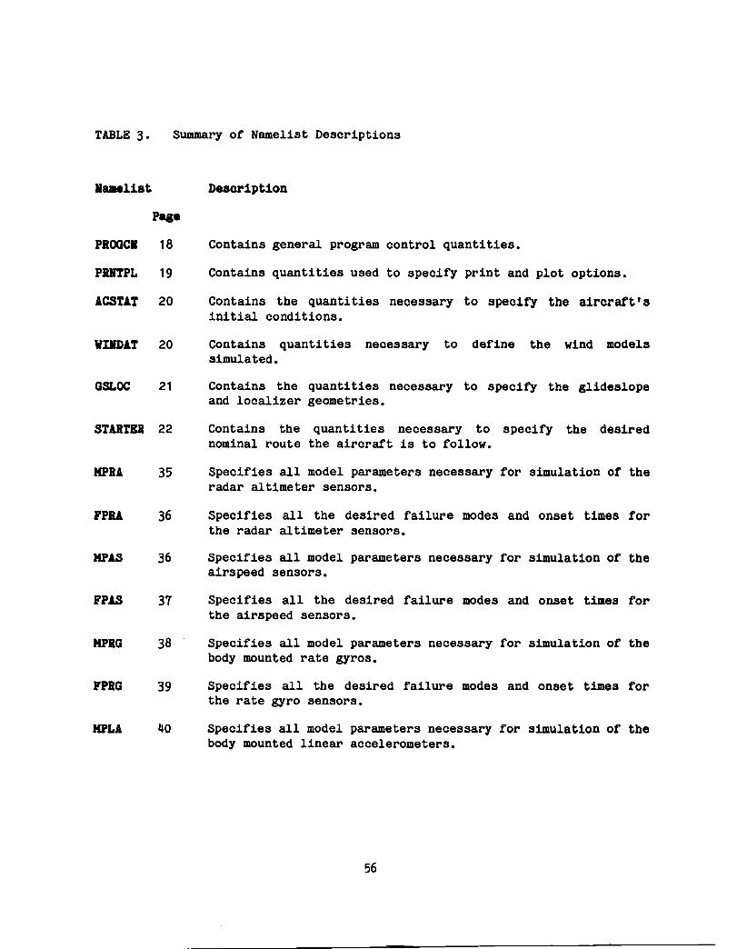
TABLE 3.

1I •• list

PROGCI

PUl'PL

ACSTAT

WIIDAT

GSLOC

STARTBB

MPRA

'PIlA

MPAS

'PAS

MPRG

'PRG

MPLA

Summary of Namelist Descriptions

Page

18

19

20

20

21

22

35

36

36

37

38

39

40

Desoriptioll

Contains general program control quantities.

Contains quantities used to specify print and plot options.

Contains the quantities necessary to specify the aircraft's initial conditions.

Contains quantities necessary to define the wind models simulated.

Contains the quanti ties necessary to specify the glideslope and localizer geometries.

Contains the quantities necessary to specify the desired nominal route the aircraft is to follow.

Specifies all model parameters necessary for simulation of the radar altimeter sensors.

Specifies all the desired failure modes and onset times for the radar altimeter sensors.

Specifies all model parameters necessary for simulation of the airspeed sensors.

Specifies all the desired failure modes and onset times for the airspeed sensors.

Specifies all model parameters necessary for simulation of the body mounted rate gyros.

Specifies all the desired failure modes and onset times for the rate gyro sensors.

Specifies all model parameters necessary for simulation of the body mounted linear accelerometers.

56

Table 3. Summary of Namelist Descriptions, concluded

M ... list Desoription

FPLl

MP1G

FPAG

FPML

MPGR

FPGB

FDIGR

MPlR

FPAR

FDIAB

Page

41

42

43

Specifies all the desired failure modes and onset tiDles for the linear accelerometer sensors.

Specifies all model parameters necessary for simulation of the body mounted attitude gyros.

Specifies all the desired failure modes and onset tiDles for the attitude gyro sensors.

44 Specifies all model parameters necessary for siDlulation of the microwave landing system (HLS) receivers.

46

47

48

49

50

51

52

Specifies all the desired failure modes and onset times for the MLS sensors.

Specifies all model parameters necessary for simulation of the redundant strapdown inertial measurement unit's

Specifies all the desired failure modes and onset tiDles for the RSDIMU rate gyro sensors.

Specifies the failure detection and isolation algorithms to be used by the rate gyros in the RSDIMU module.

Specifies all model parameters necessary for simulation of the RSDIMU two-degree-of-freedom linear accelerometers.

Specifies all the desired failure modes and onset times for the RSDIMU linear accelerometer sensors.

Specifies the failure detection and isolation algorithms to be used by the linear accelerometers

FILTDI 53 Contains the quantities needed to initialize the fault tolerant navigator.

57

TABLE 4. Summary ot • IHP Files

FILl-IAMB VARIABLE NAMES [ (rows,columns) ]

NAHELIST NAKE:

GBIIIlW..DP

ACST!T:

WINDAT:

PROGCN:

PRNTPL:

GSLOC:

STARTER:

SBllSOB.I1P

MPRA:

FPRA:

MPAS:

FPAS:

MPRG:

PITCH, ROLL, YAW, RINLO, RINLA, AIRSPE, HIGHT, WEIGHT, CG, RHO, THRUST, RE, PDEG, QDEG, RDEG

GUST, IGUST, SCALEW, SDSUBW, SHEAR, SH1, SH2, WINDSS, PSIW

TIME, FILTER, lEST, TSTOP, YSTOP

PLOTS, OUTPS, IHEAD, IPRNT, KPRINT, NTICK, CPUCHK

GPIPRN, LOCRAN, PSIR, THETAG

NW, WLO(NW), WLA(NW), SLO(2), SLA(2), SHZ(2), HG(NW), VGD(NW), RT(NW-2), NEWPTH, KPATH, IC, TANLIM, SNDP(NW-2)

IDRA, IREPRA, DTRA, SDNRA(IREPRA), SDBRA(IREPRA), SLIMRA

FINRA, FIBRA, FRRA, TFRA(IREPRA,5)

IDAS, IREPAS, DTAS, SDMNAS(IREPAS), SDBAS(IREPAS), SLlMAS

FINAS, FIBAS, FRAS, TFAS(IREPAS,5)

IDRG, IREPRG, DTRG, SDNRG(IREPRG*3), SDBRG(IREPRG*3), SDSFRG(IREPRG*3), SLIMRG(3), SDTMRG(6)

58

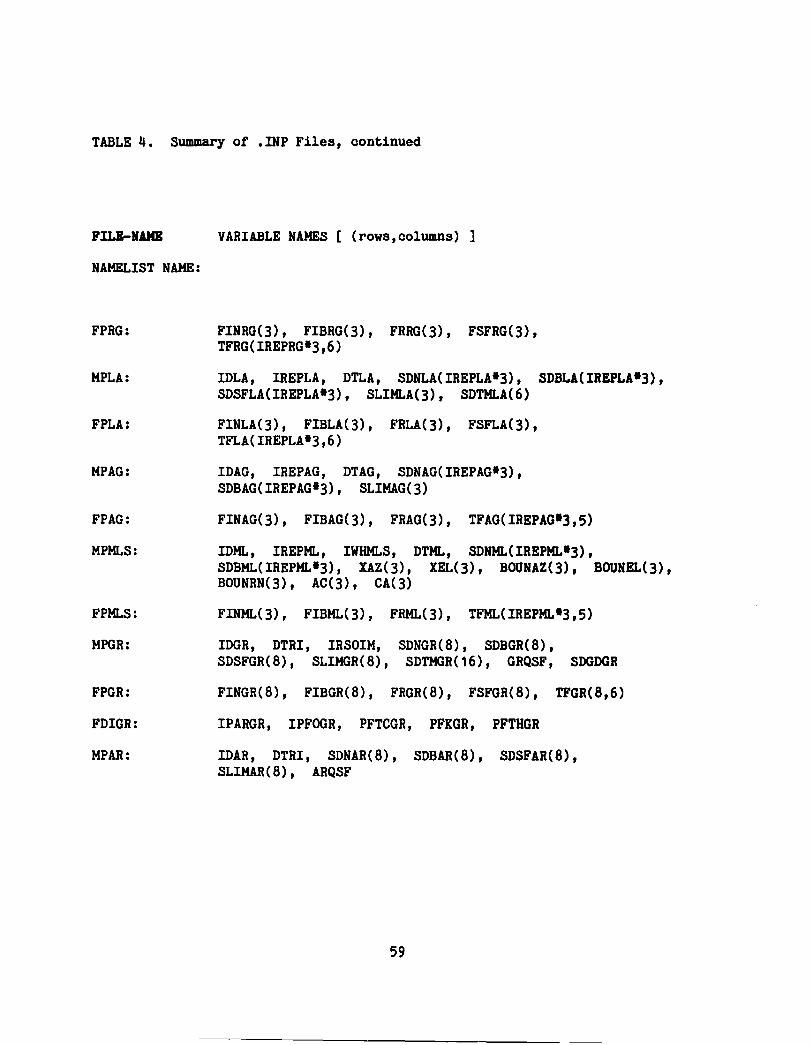
TABLE 4. Summary of .INP Files, continued

FILE-IAMB

NAMELIST NAME:

FPRG:

MPLA:

FPLA:

MPAG:

FPAG:

MPHLS:

FPHLS:

MPGR:

FPGR:

FDIGR:

MPAR:

VARIABLE NAMES [ (rows, columns) ]

FINRG(3), FIBRG(3), FRRG(3), FSFRG(3), TFRG(IREPRG·3,6)

IDLA, IREPLA, DTLA, SDNLA(IREPLA.3), SDBLA(IREPLA.3), SDSFLA(IREPLA.3), SLIHLA(3), SDTHLA(6)

FINLA(3), FIBLA(3), FRLA(3), FSFLA(3), TFLA(IREPLA·3,6)

IDAG, IREPAG, DTAG, SDNAG(IREPAG.3), SDBAG(IREPAG.3), SLIHAG(3)

FINAG(3), FIBAG(3), FRAG(3), TFAG(IREPAG.3,S)

IDHL, IREPHL, IWHHLS, DTHL, SDNHL(IREPHL.3), SDBML(IREPHL·3), XAZ(3), XEL(3), BOUNAZ(3), BOUNEL(3), BOUNRN(3), AC(3), CA(3)

FINHL(3), FIBML(3), FRML(3), TFML(IREPHL.3,S)

IDGR, DTRI, IRSOIM, SDNGR(8), SDBGR(8), SDSFGR(8), SLIMGR(8), SDTMGR(16), GRQSF, SDGDGR

FINGR(8), FIBGR(8), FRGR(8), FSFGR(8), TFGR(8,6)

IPARGR, IPFOGR, PFTCGR, PFKGR, PFTHGR

IDAR, DTRI, SDNAR(8), SDBAR(8), SDSFAR(8), SLIHAR(8), ARQSF

59

TABLE 4. Summary of .INP Files, concluded

NAHELIST NAME:

FPAR:

FDIAR:

FILTlT.IlfP

FILTIN:

VARIABLE NAMES [ (rows,columns) ]

FINAR(8), FIBAR(8), FRAR(8), FSFAR(8), TFAR(8,6)

IPARAR, IPFOAR, PFTCAR, PFKAR, PFTHAR

ICNTRL, lIMOF, IRSDF, IRSDFY, INOBPS(NBMXI), WINDOW, KMXEWH(NFMAX), KMXHLR, SIG(NDISTB+NYMAX+2), PBFOI(NFMAX), PBFIC(NFMAX), SDXIC(NX), SDPIC(NX), PRIORI(NFMAX), PRIORJ(3), POSBND, VELBND, ANGBND, BTHRSH(NFMAX), FTHRSH( NFMAX) , HRADAR

60

3.6 Saaple Input File Speoification

In this section, the input files for a typical FINDS run are given. The

files are discussed by way of interpretive comments attached to various lines

in each of the .INP files. Comments will be separated by w._ and will be in

bolded text in the rest of the section.

allowed in the actual namelist files.

61

Incidentally, comments are .Il2t.

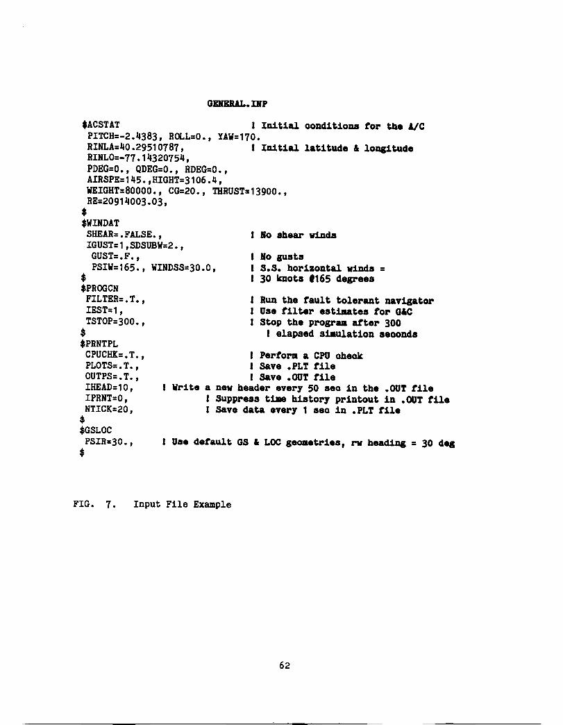
GDBJW..IIIP

$ACSTAT PITCH=-2.4383, ROLL=O.,

I Initial oonditioDB tor the Ale YAW=170.

RINLA=40.2951 0787, RINLO=-77.14320754,

I Initial latitude • 10D81tude

PDEG=O., QDEG=O., RDEG=O., AIRSPE=145.,HIGHT=3106.4, WEIGHT=80000., CG=20., THRUST=13900., RE=20914003.03,

$ $WINDAT SHEAR=.FALSE., IGUST=1,SDSUBW=2., GUST=.F. , PSIW=165., WINDSS=30.0,

$ $PROGCN FILTER=.T., IEST=l, TSTOP=300. ,

$

10 ahear winds

I 10 gusts I S.S. horizontal winds = I 30 knots .165 degrees

I BUD the tault tolerant Il&T1gator I Use tilter estimates tor O&e I Stop the program atter 300

I elapsed simulation aeoonda

I Pertorm a CPU check I SaTe .PLT tile I SaTe • OUT tile

$PRNTPL CPUCH!{= • T. , PLOTS=.T., OUTPS=.T., lHEAD=10, IPRNT=O, NTICK=20,

Write a new header every 50 sea in the .OUT tile

$ $GSLOC PSIR=30. ,

$

I Suppress t1Jle history printout in • OUT tUe I SaTe data eTery 1 sea in .PLT tile

Use detault GS • LOC .eoaetries, rv head1Dg = 30 de.

FIG. 7. Input File Example

62

$STARTER I Define the tU.ght path NEWPTH= 1, NW=4, I Two heac11Dg ohaqes in gd trk WLO(1)=-77.14538380, WLO(2)=-77.13148869, I LoDg1tu4ea ot varpo1D~a WLO(3)=-77.05845224, WLO(4)=-77.02320521, WLA(1)=40.29759451, WLA(2)=40.23788553, WLA(3)=40.20574384, WLA(4)=40.25237254,

I Latitudea ot 1f81POin~s

HG(1)=3263.3,HG(2)=2102.4, I Altitudes ot W8Jpoints HG(3)=953.9,HG(4)=.O, VGD(1)=145.,VGD(2)=135., VGD(3)=125.,VGD(4)=125., RT(1)=7500.,RT(2)=7500., IC(1)=O, IC(2)=O, SNDP=-1. ,-1. , SLO(2)=-77.025, SLA(2)=40.25, SHZ(2)=O.,

I Dea1reci airspeecl • W8JP0ints

I laciiua ot turns WLO " ¥LA are corner points Both turns are lett handed Loag, Lat, " altitude ot HLS

KPATH=2, I Use oontinued track path ooaatruotion TANLIM=O. , I Use UATHa2 at all t1aes $

$MPRG IREPRG=2,

$ $FPRG $ $MPLA

IREPLA=2, $ $FPLA $ $MPAG

IREPAG=2, $ $FPAG $

SEIISOI.DlP

I Two replicatiOns ot rate gyros, all other par_tars are cletaultecl. 110 rate gyro tailures to be s1llulatecl

Two replioatioaa ot linear aooelero.etera

I Two replioations ot attitude gyroa

FIG. 7. Input File Example, continued

63

$MPRA IREPRA=2, $ Tvo replioatiolU1 ot radar al tiMtera $FPRA $ $MPAS IREPAS=2, $ 1 Two replioat101U1 ot airspeed iDd1oatora $FPAS $ $HPGR IRSDIM=l, $ Do not st.ulate the ISDIHD $FPGR $ $FDIGR $ $MPAR $ $FPAR $ $FDIAR $ $HPMLS IREPML=2, 1 Two replloaUolUI ot IlLS SDBML(3)=4.0, SDBHL(6)=4.0, $ 1 Use _ H nob on HLS range $FPMLS FIBML(2)=8.0,TFML(5,2)=75.0, introduoe a 5 s1gaa biaa tailure OD the $ I second replication ot elevation at 75 seo.

FILTRT.DP

$FILTIN IRSDF=O, IFilter uses body aounted inputs and lIHUF=l, 1 inolude. the IHU outputs aa .. aaur_nts. INOBPS=1,2,3,4,5,6,19-0, Ilequest that x,1 and z aooel.

I as well as P,Q,R, gyro biases be identitied SIG(4)=0.0894, SIG(5)=0.0894, SIG(6)=0.0894, I set P,Q,I Doi.e level. SIG(13)=0.251, SIG(14)=0.251, SIG(15)=0.251, 1& IMD noi.es PRIORI=5-4.6E-9, 4.6E-10, 3-3.5E-9, 3.15E-8, I .et prior prob 2-2.25E-8, 2.25E-9, 3.5E-10, 17-0.0, PRIORJ=3-1.225E-19, 7-0.0, $

FIG. 7. Input File Example, concluded

64

4. DESCRIPTION OF OUTPUTS

This chapter examines the outputs available from FINDS. Each of the four

major output files, summarized in Chapter 2, will be discussed in the

succeeding sections. The sections are organized into a discussion section and

a notated sample listing of the file. The comments will be separated by"."

and will appear bolded in this chapter.

4.1 SUIIIIUU"y File

The summary file (file ext=. SUM) is an ASCII text file. It contains a

summary of the key parameters used to generate the run (from the fault

tolerant system's point of view). The file is organized into five tables

which summarize the sensor/failure models and fault tolerant system modules.

If a failure is detected, additional information is printed to clarify the

filter/detector operation at that instant of time. At the end of the listing,

if requested, a CPU summary is provided. This summary simply shows the total

CPU time used by FINDS, along with a breakdown of the fractional contributions

to it by module.

The following notated sample listing, generated by running FINDS using

the input data from section 3.6, further describes this file.

65

FINDS Version 3.0 (d.p.)

14-SEP-83 08:54:29 STANDARD SENSOR CONFIGURATION SINGLETON BIAS FAILURES -- level = 10 sigma n.o.b. TIME= 75 110 150 220 253 TYPE= el-2

Random number seed = • 32069 Integration time interval = 0.050 seconds Guidance & Control logio driven by the FILTER

INPtrT FILES USED: General Program Control:DRAl:[RLANCRAFT.RUNS1GENERAL.INP;2 Sensor Model Data: DRAl: [RLANCRAFT.RUNS1SENSOR.INP;1 Filter-Detector Data: DRAI: [RLANCRAFT.RUNSIFILTRT.INP;2

OUTPUT FILES GENERATED: General Output: Summary Output: Plot output: Time Line Output:

DRAl:[RLANCRAFT.RUNSIFINDSR.OUT;1 DRAl: [RLANCRAFT.RUNS]FINDSR.SUM;l DRA1: IRLANCRAFT.RUNS]FINDSR.PLT;1 DKAl:IRLANCRAfi.RUNS]FINDSR.TLN;1

Steady state winds = 30.000 knots at 165.00 degrees (from North) There are scheduled failures in this run

FIG. 8. Sample Summary File

66

TABLE I : SENSOR MODEL PARAMETERS

:sen;or-rype- Units Noise Level Bias Le.el Scale Factor Stop Limits I Replication (Std. De •. ) ( 7. )

Body Mounted -Accelerometers

X I I mls/s Y I I mlsls Z I I m/sls X I 2 m/sls Y I 2 m/sls Z I 2 mlsls

Body Mounted -­Rate Gyros

P I I Q I I R I 1 P I 2 Q I 2 R I 2

M. L. S • ••• Azml 1 EI I I Rngl 1 Azml 2 EI 12 Rngl 2

deg/s deg/s deg/s deg/s deg/s deg/s

deg des m

deg deg

m

9.8006E-02 9. 8066E-02 9.8006E-02 9.8066E-02 9.8006E-02 9.8066E-02

2.0000E-02 2.0000E-02 2.0000E-02 2.00(K)E-02 2.0000E-02 2.0000E-02

3.000eE-02 3.0000E-02 3.0000E+00 3.0000E-02 3.0000E-02 3.0000E+00

2.014IE-01 6. 6280E-03

-5. 7531E-03 -1.406IE-01 2. 32 16E-02

-I .4968E-0 1

-2. 3726E-05 4.8488E-05

-7. 7594E-06 -4.222IE-05 -2.6633E-05 -I .5924E-05

3. 8437E-02 -4. 4473E-02 7. 4070E+00

-9.8190E-03 5.6108E-02 6. 9795E+00

3. 5479E-0 I -6. 6226E-0 I -\. 9329E-01

1.5305E-02 1.2125E-02

-2. 8674E-0 I

5.1733E-{)4 - \. 4305E-02

1.0958[-02 9.3981E-03 1.4372E-02 4.1667E-03

N/A N/A N/A N/A N/A N/A

4.9033E+00 4. 9033E+00 1.9613E+01 4. 9033E+00 4. 9033E+00 1.9613E+01

I.OOOOE+02 I.OOOOE+02 1.000eE+02 1.0000E+02 I.OOOOE+02 1.0000E+02

N/A N/A N/A N/A N/A N/A

---------------------------------------,----Indicated •••• Airspeed (upper/lower)

2.0578E+02 5.1444E+01

IASI 1 m/s 2.0000E+00 3. 9299E-01 2.0000E+00 2. 5764E-Ol

N/A N/A IASI 2 m/s

I. M. U. phil 1 thel 1 psil 1 phil 2 thel 2 psi! 2

deg des deg des des des

2. 3000E-O 1 2.3000E-01 2.3000[-01 2.3000E-01 2.3000E-01 2. 3000E-O 1

1.8383E-02 6.0136E-02

-5. 4620E-02 7.2554E-02

-8.6147E-02 - 1 • 3620E-0 1

N/A N/A N/A N/A N/A N/A

8.0000E+01 8. OOOOE+O 1 6.0000E+02 8. OOOOE+O 1 8. lJe00E+0 1 6. OfJOOE +02

--------------------------------Radfir Al t imeter RA 11m RA 12m

3. 0480E-0 1 -2.0271E-Ol 3.0480E-01 -3.3161E-01

N/A N/A

N/A N/A

FOOTNOTES TO TABLE I :

• Body mounted accelerometers are also misaligned by the following transformation:

TMLA = 1.0000E+OO -3.6228E-03 3.3961E-03 1.5940E-02 1.0000E+OO 1.421IE-02 2. 5820E-03 1.5736E-03 I.OOOOE+OO

•• Body mounted rate gyros are also misaligned by the following transformation:

TMRG = 1.0000E+OO -7.4602E-03 -7. I 255E-03 -4. 5203E-03 1.0000E+OO -3.4715E-03 -1.5571E-03 -9.6759E-03 I.OOOOE+OO

••• M.L.S. noise is TIME CORRELATED

•••• Since indicated airspeed noise is multiplicati.e. the standard deviation of the noise is expressed in percen t (7.).

FIG. 8. Sample Summary File, continued

67

Failure Type

INC. BIAS

Fai lure Ma,ni tude

2.4000E-01

Ons.t Ti ••

80.571

TABLE II NO-FAIL FILTER STATE INITIAL CONDITIONS

States: x-rw 8.718SE+OO 4.0000E+01 m y-rw 6.4227E+OO . 4.0000E+OI m z-rW -2.2SS9E+OO 3. OOOOE+0 I m x-dot-rw -S.9S24E-01 4.0000E+OO IVS y-dot-rw -1.86SIE+OO 4.0000E+OO m/s z-dol-rw 1.8234E+OO 1.2SOOE+OO mls phi -2. 7424E-02 S.OOO0E-Ol de, theta -1.OS36E-OI S.OOOOE-OI de, psi -7.S294E-03 1.S000E+OO de, x-wind-rw 4.S72IE-02 7.S000E-OI mls y-wind-rw 3. 8239E-O I 7. 50OOE-OI m/s

Avo. Biases: x-aeeel 1.6S7IE-OI 3.0480E-OI m/s/s y-aeeel -1.44S7E-OI 3. 0480E-O I m/s/s z-aeeel 1.IOO9E-02 3. 0480E-O I m/s/s P-,yro 1.7914E-04 2.5600E-OI de,ls Q-gyro -S.SSI9E-OS 2. 56OOE-OI deg/s R-uro -1. 3474E-04 2. 56OOE-O I de,/s

TABLE III NO-FAIL FILTER NOISE AND INITIAL BIAS LEVELS

Variable--- Noise S.D. Ave. Bias Per Repl.

Noises: Process x-aeeel y-aceel z-aeeel P-gyro Q-gyro R-gyro x-wind-rw y-wind-rw

Measurement MLS azim M1.." e I MLS rn, lAS IMU phi IMU the ta IMU psi Radar al I

9. 8066E-02 1.6S71E-OI 9.8066E-02 ·-1.44S7E-OI 9.8066E-02 1.IOO9E-02 8. 9400E-02 1. 79 14E-04 8.9400E-02 -S.SSI9E-OS 8.9400E-02 -I. 3474E-04 O.eoGOE+OO NIA O.OOOOE+OO N/A

Noises: 6.0000E-02 6.0000E-02 6.0000E+OO 1.4919E+OO 2.SIOOE-Ol 2.S100E-OI 2.SIOOE-OI 3.0480E-OI

1.4309E-02 S.8176E-63 7.1933E+OO 3.2S3IE-Ol 4.S469E-02

- 1 .300SE-02 -9.S411E-02

O.OOOOE+OO

Repl iealions Used

1 1 1 1 1 1

N/A NIA

2 2 2 2 2 2 2 0

FIG. 8. Sample Summary File, continued

68

Uni Is

mlsls m/s/s m/s/s deg/s des/s de,ls m/s m/s

de, de, m

m/s de, de, de, m

TABLE IV : DETECI'OIl RESET , AlWlETEIS

Detectors asso.e I.L.S •• oise is COLORED Deteotor Window Le.,th· I.eeeee Secoad.

Sensor T,pe

'priori 'rob ESt. Wi.dow Esli.alio. 0.11.

Sin,olar Failores: x-accel 4.6890£-99 y-accel 4.6890£-99 z-acoel 4.6000E-99 '-,yro 4.6090E-99 Q-,yro 4.6000E-99 R-Iyro 4.6000E-19 illS azi. 3.seoa£-99 illS e I 3. S0OO£-99 illS rn, 3.S000£-99 lAS 3.1500£-98 IIIU phi 2.2500£-98 IIIU theta 2.2509£-98 IIIU psi 2.2590£-99 Radar alt 3.seee£-19

(Iec) I.tor •• tlo.

3.eeeee 3.eeeee 3.00eee 3.eeeee 3.eeeee 3.eoooo I.eoooo I.eoooo I.eoooo I.ooeoo I.eeeee I.ooeoo 1.00000 I.eeeee

(S.D.)

9.2993£-83 9.2993£-83 9.2993£-83 9.9OO9E+ee 9.eeeo£+ee 9.eooe£+ee 9.eeoo£+ee 9.0009E+ee 9.eooe£+00 9.eooe£+00 9.9999E+ee 9.9999E+ee 9.9999E+ee 9.9999E+00

Siloltaneool loltiple Failores: illS azi. 1.2250£-14 illS el 1.22S0£-14 illS rn, 1.2250£-14

TABLE V : SENSOR HEALER , AlWlETEIS

ae.ler Window Len,th • 3.0000e Seeonds

SeDsor Bias Est Failore Est DecisioD Thresold Threshold Threshold

a/s/s a/./. a/s/s de,/. de,/s de,/s de, de, • a/s

de, de, de, •

O.its Type

(Sqoare U.i ts)

I-acoel 2.eeoo£-01 5.0000£-91 -1.1327£-91 a/s/s 1-ac ool 2.0000£-91 5.0000£-01 -1.1327£-01 a/I/S z-accel 2. eooe£-0 I 5.0000£-01 -1.1327£-01 a/s/s P-uro 1.2000E-93 1.2000E-02 -4.71 I IE-83 de,/s Q-nro 1.2000£-03 1.2000£-02 -4.7111£-93 de,/s Ri]yro 1.2000£-03 1.2000£-02 -4.71 11E-03 de,/. II azi. 6.0000E-02 1.S000£-01 -2.I200E-02 de, illS e I 6.0000£-02 I.seee£-Ol -2. I200E-02 de, illS rn, 1.2000E+OI 2.eeooE+OI -2. I 290E+92 • lAS 1.2000E+OO 2.seeo£+00 -1.3197E+01 a/s IIIU phi 2.0000E-OI 5. OOOOE-O I -3. I I 52E-0 I de, IIIU theta 2. OOOOE-O I 5.0000£-01 -3. I I 52E-01 de, IIU psi 2. OOOOE-0 I 5.0000£-01 -3. I I 52E-0 I de, Radar alt 6.1000£-01 l.seee£+OO -5.4799£-01 •

FIG. 8. Sample Summary File, continued

69

DECIDE: Sensor type MLS el • Replication No.2 Failed at time= 81.000 Estimated Failure Level 3.23494907E-03 deg

ALAMDA I. 296D.e2 I. 276D.02 I. 249D+02 I. 4OOD.02 I. 344D+02 I .341 D.02 I. 286D.02 I. 263D.02 I. 286D+02 I. 268D+02 1.26ID+02 1.278D+02 1.296D.02 9.990D+30 1.283D+02 1.039D.e2 1.285D+02 1.266D.02 1.31ID+02 1.276D+02 1.306D+02 9.99OD+30 1.090D+02

ALAMDJ 1.410D+02 1.334D+02 1.41ID+02 PO BEFORE 6.840D+00 7.243D+00 8.686D+00 5.05ID-OI 3. 690D-0 I

5.72ID-01 1.047D-08 1.043D-08 1.05ID-08 4.675D~01 2.936D-OI

V mi :-2. 738D+02-6.853D.0 I 4.260D+03-4.389D+01-2.109D+01 7.766D+02-1.338D-03-7.316D-05-3.090D-053.039D+OI 2.73ID+01-6.716D-01 5.330D+00-1.852D+OI 5.S09D-05

-2.043D-05-2.745D-06 PB BEFORE 2.670D-03 2.837D-03 2.972D-03 6.I54D-II 6.227D-II

6.070D-11 PO AFTER 7.638D+00 7.293D+00 2.017D+02 5.256D-OI 3.737D-OI

6.988D+00 1.049D-08 1.043D-08 1.05ID-08 4.774D-OI 3.0ISD-01

PB AFTER 2.675D-03 3.140D-03 6.620D-03 6.157D-II 6.228D-II 6.070D-II

GLIDESLOPE CAPTURE AT TIME = 157.40

GLIDESLOPE CAPTURE PLUS 10 AT TIME = 167.35

LOCALIZER ONCOURSE AT TIME = 192.25

• BEGIN DECRAB AT TIME = 245.05 • Radar Animeter turn-on at t= 251.70 PO BEFORE 2.31ID+00 1.587D+00 2.632D-OI 2.336D-01 3.233D-01

1.783D-OI 2.207D-09 2.206D-09 2.218D-09 4.967D-03 4.615D-03

V mi O.OOOD+00 O.000D+00 O.000D+OO O.000D+00 O.000D+00 O.OOOD+00 O.OOOD+00 O.000D+00 O.000D+00 O.000D+00 O.OOOD+00 O.000D+OO O.000D+00 O.OOOD+OO O.000D+00 0.000D+00 O.OOOD+OO

PB BEFORE 4.912D-04 5.036D-04 5.530D-04 8.66ID-13 8.665D-13 5.827D-13

PO AFTER 2.31ID+00 1.587D+00 2. 632D-0 I 2. 336D-0 I 3. 233D-01 1.783D-01 2.207D-09 2.206D-09 2.218D-09 4.967D-03 4.6ISD-03

PB AFTER 4.912D-04 5.036D-04 5.530D-04 8.66ID-13 8.665D-13 5.827D-13

CAT II DECISION HEIGHT AIRCRAFT HEIGHT = 99.94 AIRCRAFT LATERAL DEVIATION z -2.15 AIRSPEED ERROR = 0.22 GLIDESLOPE OFFSET = 199.56 TIME = 251.750 SEC

• BEGIN FLARE AT TIME = 257.15 • ENDPOINT DISPERSION DATA HIGHTR = 0.16 XPOS 1324.81 YPOS. -0.54 HOOT = -3.04 AIRSPEED=. 195.49 TIME 264.950 SEC

FINAL POSITION 1.3248E+03 -5. 3835E-0 I -9.8967E+00 END EXECUT ION

FINDS CPU USAGE SUMMARY

Total CPU time spanned = Initialization = A/C simUlation + Plots = Sensor model simulation Faul t tolerant fi Iter =

5622.00 seconds 0.06 7. 4.71 7.

CPU Breakdown for Fault Tolerant Initialization + misc. = No-Fail Filter = . Bank of Detectors + LR compo = Decision. healing. & reconf =

I. 78 7. 93. II 7.

Fi Iter: 0.63 7.

30.41 7. 68.52 7. 0.43 7.

CPU Breakdown for Bank of Detectors & LR computers Initialization and overhead 40.787. Inner loop set-up = 29.58 7. Detectors = 12.767. LR l'omputers = 14.31 7. Multiple detectors + HO 2.577.

FIG. 8. Sample Summary File, concluded

70

'.2 Tta. LiD. rile

The discrete time line file (file ext=.TLH) is a variable length

formatted ASCII file. 5 It attempts to oapture the disorete nature of the

automated approach and landing environment. 'lbe tile oonsists ot ooded

information stored in a fixed format. Whenever an -event- ooours, (suoh as

glideslope capture or a simulated failure) a coded -snapshot- of important

variables are recorded. This file can be used to obtain statistioal

information, (when combined with other .TLH tiles trom a Monte carlo

simulation), about FINDS failure detection performanoe (false alarm rate,

average time to detect, etc.) as well as estimation and slst- performanoe

measures at particular points in the tlight path.

Tbe time line tile is organized into a header record, whioh identities

the file type; a number of records of comment lines (the number is determined

from the header record); and a sequence of three (3) reoord disorete

snapshots. Each "snapshot" consists of the following items:

o Time of occurrence

o A coded integer representing the discrete event

o Four (4) integer descriptors (I.D.) which further olarity the event

o Eighteen (18) floating pOint descriptors (F.P.D.)

Table 5 defines the last three items for each discrete event. However, in

order to interpret the table properly, a few oomments are needed:

o integer descriptor #4 specifies the following: O=>F.P.D.s are

5In order to reduoe disk storage reqUirements (a signifioant oonsideration in Monte Carlo studies), future releases of FINDS should store tbis tile in an unformatted (binary) fashion.

71

absolute values, 1=>F.P.D.s are errors (true-estimated). I.D. ,_ is therefore not included in Table 5.

o The following nbasicn floating point description outputs are available, to choose from (coded A -> F):

A: Xrw,Yrw,Zrw,Zrw,Airspeed

B: Azm,El,Rng

c: Xrw' Yrw ' Zrw

D:Xrw'Yrw'Zrw'Xrw'Yrw'Zrw,-,e,t, ~'Yw,Airsped error from desired, crosstrack error from desired, altitude error from desired

E:D+F.P.D(17) = estimated singular failure level + F.P.V. (18) = uncertainty in estimate

F: D+F.P.D (15) = first multiple failure level, +F.P.D (16) = uncertainty in FPD (15) +F.P.D (17) = second multiple failure level, +F.P.D (18) = uncertainty in F.P.D (17).

o A blank entry in the table signifies the descriptor is not used.

o Failure type is coded as 1=>increased noise, 2=>bias, 3=>scale factor, 4=>hardover, 5=>null, 6=>ramp failures.

o Table 1 on page 9 defines the sensor type index

}

72

TABLE 5. Summar1 or Tille Line Codes

Event Name Event I I.D.I1 I.D.I2 I.D.I3 F.P.D. Format

Begin Run 1 lEST , End Run 2 , MLS Turn-on 3 B

Filter- 4 ICNTRL IDlJF IRSDF C detector Turn-on

RA Turn-on 5 D

G.S. Capture 6 A

G.S. Capture 7 D plus 10

LOE on course 8 D

Begin Decrab 9 D

Begin Flare 10 D

CAT II 11 D Decision height

Not Used 12

Not Used 13

Failure Onset 14 rallure sensor sensor D t1pe t1pe rep.

73

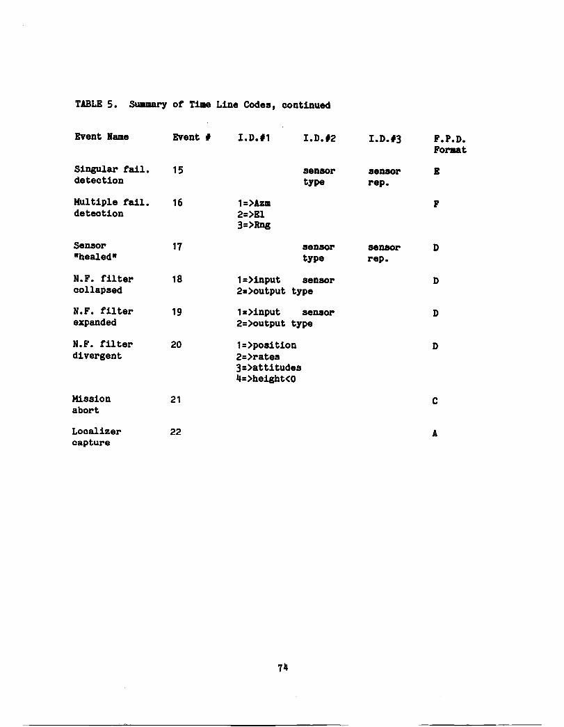
TABLE 5. Suamary ot Time Line Codes, continued

Event Bame Event' I.D.'l I.D.'2 I.D.'3 F.P.D. Forat

Singular tail. 15 sensor sensor E detection type rep.

Mul tiple tail. 16 l=>AZII F detection 2=>El

3=>RDg

Sensor 17 sensor sensor D -healed- type rep.

H.F. filter 18 l=>input sensor D collapsed 2=>output type

B.F. tilter 19 l=>input sensor D expanded 2=>output type

H.F. filter 20 l=>position D divergent 2=>rates

3=>attitudes 4=>he1ght<0

Mission 21 C abort

Localizer 22 A oapture

The following sample time line file, Figure 9, was generated using the

input files defined in Figure 7 on page 62.

To help the reader understand this important file, lets discuss three

snapshots, marked A,B,C in Figure 9.

A

B

C

This snapshot marks the filter/detector algorithm start-up. Notice that the event occurs at Time= 35.25 seconds, and that the A/C's position is: Xrw=-3116 H, Yrw=-9311 H, Zrw=-806 H.

This event represents the simulated increased bias failure of the second replication of HLS elevation. The event happens at Time=80.6 seconds.

Here we see that at 81 seconds the decision logiC has declared the second replication of HLS elevation to be faulty, and removed it from the problem. Notice that the estimated failure level is 0.185 degrees. By compairing C to B we see that it took .4 sec. to detect this failure.

Based on the information contained in this file several useful measures

can be defined. For example, in a single run the following items could be

compaired or computed:

o Time to correctly detect a failure, i.e. time of detection minus time of failure.

o Time to correctly heal a repaired sensor, i.e. time of healing minus time of incorrect failure or repair.

o Total number of false alarms, i.e. detection of a failure that wasn't simulated.

o Total number of missed detections, i.e. failure to correctly detect a failure.

o Total number of incorrect healings.

o State estimation error at various pOints in the run.

o Performance errors at critical points in the run.

By computing the above quantities for each run, and averaging or summing

75

FINDSR.TLN; 1 20-SEP-I983 09:35 Pale 1

TLNI 4 STANDARD SENSOR CONFIGURATION SINGLETON BIAS FAILURES -~ 1eye1 = 10 sigma n.o.b. T IME= 75 110 150 220 253 TYPE- el-2

0.0000 1 1 0 0 0-6.6355E+02-1.1201E+04-9.3696E+023.2496E+00 7.4594E+01 0.0000E+00 0.0000E+00 0.0000E+00 0.0000E+00 0.0000E+00 0.0000E+00 0.0000E+00 0.0000E+00 0.0000E+00 0.0000E+00 0.0000E+00 0.0000E+00 0.0000E+00

35.2500 3 0 0 0 0 5.8184E+01 4.6151E+00 1.0959E+04 0.0000E+00 O.0000E+00 O.0000E+00 O.0000E+00 0.0000E+00 0.0000E+00 O.0000E+00 O.0000E+00 O.0000E+00 O.0000E+00 O.0000E+00 O.0000E+00 O.0000E+00 O.0000E+00 O.0000E+00

35.2500 4 0 1 0 0-3. 1163E+03-9.3111£+03-8.0674E+02 O.0000E+00 ----A O.0000E+00 0.0000E+00 O.0000E+00 O.0000E+00 0.0000E+00 O.0000E+00 0.0000E+00 O.0000E+00 0.0000E+00 O.0000E+00 O.0000E+00 O.0000E+00 O.0000E+00 0.0000E+00

80.6000 14 2 8 2 1 1.5203E+00 1.2454E+01 2.4628E+00-1.7391E-Ol -3.8993E-01-3.0700E-01-6.8313E-02-7.4681E-02 5.5642E-02 1.0018E+Ol-l.0417E+Ol B 8~:~E+~SI.91~5E+0~ 2.1~27E+~2~7~~~8~36~~~4~0~~~2~0e~~;~----

4. 0973E-0 1 2.9930E-02-8.2717E-02-5.9572E-02 1.8718E-Ol 9.9836E+00-1.0438E+01 C -1 . 9697E+00-1 . 9678E+Ol 4. 0353E+00 O. 0000E+00 O. 0000E+00 1. 8535E-Ol 2. 3777E-02

157.4000 6 0 0 0 0-5. 1428E+03-8.0305E+02-3.0122E+02 3.5258E+00 ----6.6te5E+Ol O.0000E+00 0.0000E+00 0.0000E+00 O.0000E+00 O.0000E+00 0.0000E+00 O.0000E+00 O.0000E+00 0.0000E+00 0.0000E+00 O.0000E+00 0.0000E+00 O.0000E+00

167.3500 7 0 0 0 0 4.9751E+00-2.0130E-01-2.3954E+00-6.5165E-01 -3. 2478E-0 1 9.2921E-02-1.3047E-01-3.2320E-02 9.6692E-02 9.4701E+00-9.6710E+00 3.2928E-02-5.9013E-Ol-l.0699E+00 O.0000E+00 O.0000E+00 O.0000E+OO O.0000E+00

192.2500 8 0 0 0 0 2.9448E+00 3.5465E+00-l.6928E+00-7.2610E-01 5. 2285E-0 1 3.8571E-02-1.4277E-01-5.6151E-02 8.7711E-02 9.9642E+00-9.4142E+00 4. 4256E-0 1 5.7629E+00 7.2765E-02 O.0000E+00 O.0000E+00 O.0000E+00 O.0000E+00

245.0500 9 0 0 0 02.2182E+00-2.6317E-01-7.1819E-01-7.7573E-01 -2. 10 49E-01-9.5215E-02 2.4582E-02 6.5698E-02 1. 1209E-02 1.0285E+01-9.0163E+00 8.7472E-02-2.0651E+00-2.9306E-01 O.0000E+00 O.0000E+00 0.0000E+00 O.0000E+00

251.7000 5 0 0 0 1 6. 1919E+00 1.3219E+00-1.8943E-01-7.0267E-01 1.3991E-01-6.3539E-02 4.3436E-02 1.3055E-Ol 2.5067E-02 1.0291E+01-8.9651E+00 3.0494E-Ol 1.9892E+00-4.0475E-01 0.0000F.+00 O.0000E+00 O.0000E+00 O.0000E+00

251.7000 18 2 8 1 1 6. 1919E+00 1.3219E+00-1.8943E-01-7.0267E-01 1.3991E-01-6.3539E-02 4.3436E-02 1.3055E-Ol 2.5067E-02 1.0291E+01-8.9651E+00 3.0494E-01 1. 9892E+00-4. 0475E-Ol 0. 0000E+00 O. 0000E+OO O. 0000E+OO 0. 0000E+OO

251.7000 19 2 14 l' 1 6. 1919E+00 1. 3219E+00-1. 8943E-01-7 .0267E-01 1.3991E-01-6.3539E-02 4.3436E-02 1.3055E-Ol 2.5067E-02 1.0291E+01-8.9651E+00 3.0494E-01 1.9892E+00-4.0475E-Ol O.OOOOE+OO 0.0000E+00 0.0000E+00 O.0000E+OO

2S 1. 7500 11 0 0 0 0 3. 4610E+00 1. 3012E+00-1. 9396E-01-7 .4006E-01 1.2394E-Ol-1.5049E-Ol 8.4812E-02 9.7071E-02-2.0560E-03 1.0291E+01-8.9642E+00 2. 6950E-01 1.9560E+00-2.7817E-Ol 0.0000E+00 O.0000E+OO 0.0000E+00 O.0000E+00

257.1500 10 0 0 0 0 3. 1236E+00 4. 5899E-01-2. 1601E-01-8.0380E-01 -1.6903E-02 2.9301E-02 8.9153E-02 1.0078E-01-5.2041£-03 1.0288E+01-8.9214E+00 2.2618E-Ol-1.0014E+00-6.6519E-01 0.0000E+00 O.e000E+00 O.0000E+OO 0.0000E+00

264.9500 2 0 0 0 0 4.0380E+02-1.6409E-01-3.0165E+00 9.4027E-01 5.9585E+Ol 0.0000E+00 O.0000E+OO 0.0000E+00 O.OOOOE+OO 0.0000E+00 0.0000E+00 O.0000E+OO 0.0000E+00 O.0000E+OO 0.0000E+00 O.0000E+OO 0.0000E+00 0.0000E+09

FIG. 9. Sample Time Line File

76

across an ensemble of like runs, statistical pertormace _asures can be

obtained.

'.3 OUtput File

The output file (file ext=.OUT) is an ASCII text file. It contains a

complete echo check of all namelist and interactive inputs and therefore

completely defines the run. It also contains as an option, a table ot time

history outputs. If OUTPS=.False., this file will not be generated. (The

default for Monte-Carlo simulation study). This file is basically used for

verification purposes.

The following sample output details this file.

11

FINDS Version 3.0 (d.p.)

14-SEP-83 08:54:29 srANDARD SENSOR CONFIGURATION SINGLETON BIAS FAILURES -- leyel - 10 sil.a n.o.b. TIME" 75 110 150 220 253 TYPE" el-2

Rando. nu.ber seed" . 32069 Intearation li.e interyal - 0.950 seconds Guidance a Control loaic driven by the FILTER

INPUT FILES U~~: General Proara. Control:DRAI:IRLANCRAFT.RUNS1GENERAL.INP;2 Sensor Model Data: DRA1:IRLAHCRAFT.RUNSISENSOR.INP;1 Filter-Detector Data: DRA1:IRLANCRAFT.RUNS1FILTRT.INP;2

OUTPUT FILES GENERATED: General Ou tpu t: Su_ary Output: Plot output: Ti •• Line Output:

DRAI:IRLANCRAFT.RUNSIFINDSR.OUT DRAI:IRLANCRAFT.RUNSIFINDSR.SUM DRAI: IRLANCRAFT. RUNS I FINDSR.PLT DRAI: IRLANCRAFT.RUNSIFINDSR.TLN

.ACSfAT PITCH · -2.438300090000000 , ROLL - 9.~E+99, YAW 179.0090999990990 RINLO - -77. I 43207S4099999 RINLA 49.29519787009990 AIRSPE · 145.0000000090000 HIGHT 3196.400000090000 WEIGHT 80000. 000000000e0 CG 20.00000000e00e00 RHO - 2.3081 I90000009000E-03: THRUsr - 13900. OOOOOOOO909 HE -. 20914993.03000000 , PDEG · 9.~E+99, QDEG 0.~E+99, RDEG - 9.~E+99 SEND SWINDAT GUsr - F, IGUsr I, SCALEW .. 1499.099009000009 SDSUBW .. 2.~ SHEAR .. F, SHI • -6. 7499999999999999E-02 , SH2 -9. 13S0000099909909 WINDSS - 39.90900009999009 PSIW 165. 0090999990990 SEND SPROGCN DTIME .. S. 000000000990999E-02 , FILTER .. T, IEsr = I, TsrOP 399.0000e00909990

ysrop 399.0000900009999 SEND .PRNTPL PLOTS T, OUTPS T, I HEAD 10, IPRNT 0, KPRINT .. 0, NTICI 2, CPUCHI • T SEND SGSLOC GPIPRN .. 1099. 0000e0000900 LOCHAN = 19999. 99999999990 PSIR 39.~ THt.'TAG .. 3. 900000000000000 aF.ND

FIG. 10. Sample Output File

78

BODY MOUNTED RATE GYRO MODEL PAlWIETER INPtITS SMPRG IDRG IREPRG DTRG SDNRG SDBRG SDSFRG SLIMRG SDTMRG SEND SFPRGI FINRG FIBRG FRRG FSFRG IFRG TFRG SEND

2, 2,

= 5.~E-02, 9-2. 000000000000000E-02 ,

= ge2.~E-05, = 9-1.~E-02,

3- 100.0000000000000 6-0.400000e000000000

BODY MOUNTED ACCELEROMETER MODEL PARAMETER INPUTS SMPLA IDLA IRErLA 2

DTLA SDNLA SDBLA SDSFLA SLIMLA SDTMLA SEND SFPLAI FINI.A FIBLA FRLA FSFLA .IFLA TFLA SEND

2. 90000900009000O

ATTITUDE GYRO MODEL PARAMETER INPUTS SMPAG IDAG IREPAG

DTAG SDNAG SDBAG SLIMAG SEND SFPAG! FINAG FIBAG FRAG I FAG TFAG SEND

2. 2,

RADAR ALTIMETER MODEL PARAMETER SMPRA lORA IREPRA DTRA SDNRA SDBRA SLIMRA SEND SFPRA! FINRA FIBRA FRRA IFRA TFRA SEND

•

•

•

600. 0000000000000

INPtITS

FIG. 10. Sample Output File, continued

79

$!,"T ARTER NW 4. WLO ,,-77.14538380000900 • -77.13148869900009 •

-77.05845224000000 • -77.92320521000000 • 6-0.~E+89. WLA 40.29759451000000. 40.23788553000000 •

40.20574384000000 • 40.25237254000000 • 6·0.~E.00. SLO = -77.16489400000000 -77 .025e0000000000 SLA 40.40301600000000 40.2S000000009000. SHZ 150.~ O.~E.OO. HG 3263.300000000000. 2102.400000000000

953.9000000000000 • 7-0.~E+00. VGD 145. OOOOOOOOOOOOO • 135. OO0OO0OO0OO00 2-125.0000e00000000 ,6-0.~E+00. RT = 4-7500.000000000000 • 4-0.000000000090000E+00. N~WPTH I. KPATH 2. IC = 4-0, 6-1. TANLIM " 0. 000000000000000E+OO. SNDP 2--1.000000000000090 6-0.000000000000000E+00 SEND SFllTIN ICNTRL " O. IIMlIF I. IRSDF 0, IRSDFY = lI. I NORPS I. 2. 3. 4. 5,

6. 19-0. WINDOW 1.000000000000000 KMXEWH = 6-3, 8-1, 11-0. KMXHLR 3. S I G = 3-9. 8066352000000002E-02, 3-8. 940000000000000E-02 • 2-0.~E.00. 2-6.~E-02. 6.000000000000090

1.491885891300010 • 3-0.2510000000000000 • 0.3048000009000090 • I ,5528249843748540E-04 , 5. 48207573443556 15E-04. 12-0.~E+OO,

PBFO I = 3-0.3048000000000000 • 3-0.2560000009000000 • 2-9. OOOOOOOOOOOOOOOE-02. 90. OOOOO0OOOOOOOO I . S0000OO0OO00000 2-0.8000000000000000 • 2.400000000000000 I • OOOO090000OO0OO I 1-0. 0000001:1000000000E+00. PBFIC = 3-0.loooooe000000OO0 ,27-0.~E.00. SDXIC = 2-15.01l000000000900 • 5.~ • 3- I .50OOO0I1()(lOO0OOO • 2-0. 1000000000000000 ,0. 200000000900090 2*0.500000U00000000 • 14*0. 000000000000000E+OO, SDPIC = Z*40.00000000000000 , 30.00000000000ee0 • Z*4.~ • 1.2SOOO0l10OOOOOOO • 2-0.500000000000000 •

1.500000000000000 ,2-0.7500000000000000 • 14*0.000000000000000E+00. PR lOR I = 5-4. 6OOI:lOO0OOO00OE-09, 4. 60OOOO000OOOOOOE-10. 3*3. 50000OOOOO0OOOOE-09. 3. 1500000000000000E-08. Z-2. 2~E-08. 2.25000000000000~')()E-09. 3.~E-IO. 17*0.~E+00.

PR IORJ 3* I . 2250000000000000E-14 • 7-0. OOOOO0OOOOOOOOOE+OO. POSBND ZOO. 0000000000000 VELBND = 30. OOOOOOOOOOOOOO ANGBND = 10.00000000000000 BTHRSH = 3*0. 21100000000000000 ,3* I • 200000000000000E-03, 2·6. 00000OllOOOOOOO(lOE-02 • 12.00000000000000 • I .200000000000000 • 3-0.2(}()()eO(-)1l1:l0000000 • 0.6100000000000000 • II*O.~E.OO, FTHRSH = 3-0. SOOOOOOOOOOOO9O • 3* I . 2OOOOOOO0OOO0OOE-02. 2-0. 15OOOOIJOOOOOe00 • 20. oooooooeoooooo • 2.500000009000000 • 3-0. soooeoooooooooo ,. I .500000000000000 • 11*0. 000000000000000E+OO. HRADAR 30.48000000000000 .F.NIJ DECIDE: Sensor type MLS el • Replication No.2 Failed at ti •• - 81.000

Estimated Failure Le,el = 3.Z3494907E-03 deg

GLIDESLOPE CAPTURE AT TIME = 157.40

GlIDESLOPE CAPTURE PLUS 10 AT TIME = 167.35

LOCALIZER ONOOURSE AT TIME = 192.25

* BEGIN DECRAB AT TIME = 245.05 • Radar Al timeter turn-oln at t= Z51. 70 CAT II DECISION HEIGHT AIRCRAFT HEIGHT 99.94 AIRCRAFT LATERAL DEVIATION - -2.15 A I RSPEED ERROR = 0 . 22 GL IDESLOPE OFFSET .. 199.56 TIME - 25 I .750 sa:

- BEGIN FLARE AT TIME = 257.15 -ENDPOINT DISPF~ION DATA HI6HTR = 0.16 XPOS 1324.81 Ypas - -0.54 HDOT " -3.04 AIRSPEED=, 195.49 TIME = 264.950 SEC

FIG. 10. Sample Output File, concluded

80

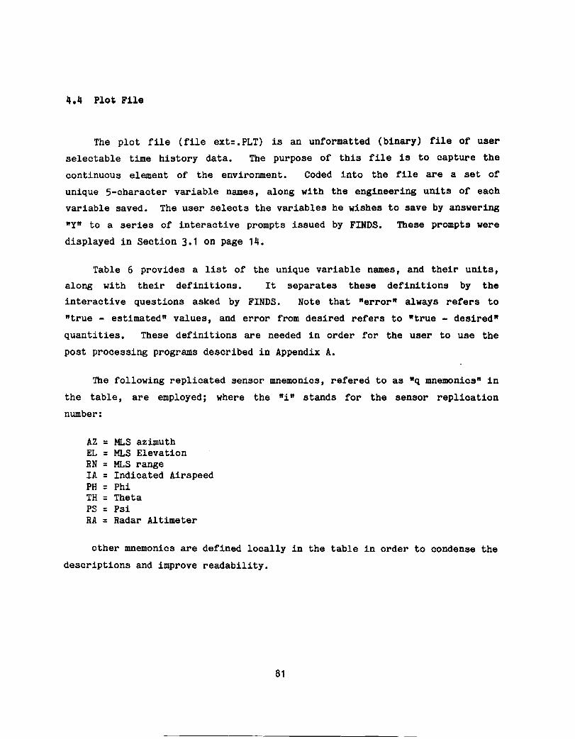
4.4 Plot File

The plot file (file ext=.PLT) is an unformatted (binary) file of user

selectable time history data. The purpose of this file is to capture the

continuous element of the environment. Coded into the file are a set of

unique 5-character variable names, along with the engineering units of each

variable saved. The user selects the variables he wishes to save by answering

"Y" to a series of interactive prompts issued by FINDS. These prompts were

displayed in Section 3.1 on page 14.

Table 6 provides a list of the unique variable names, and their units,

along with their definitions. It separates these definitions by the

interactive questions asked by FINDS. Note that "error" always refers to

"true - estimated" values, and error from desired refers to "true - desired"

quantities. These definitions are needed in order for the user to use the

post processing programs described in Appendix A.

The following replicated sensor mnemonics, refered to as "q mnemonics" in

the table, are employed; where the "in stands for the sensor replication

number:

AZ = MLS azimuth EL = MLS Elevation RN = MLS range IA = Indicated Airspeed PH = Phi TH = Theta PS = Psi RA = Radar Altimeter

other mnemonics are defined locally in the table in order to condense the

descriptions and improve readability.

81

TABLE 6. Plot File Mnemonics

Prompt1ng Question

Variable name Definition

1. No-Fail filter state est error?:

EX Xrw error

EY Yrw error

EZ Zrw error

EXD Xrw error .

EYD Yrw error .

EZD Zrw error

EPHI phi error

ETHE theta error

EPSI psi error

EXW Xw error

EYW Yw error

2. No-Fail filter state est Unoertainty?:

SDXi Standard deviation of the total, updated, state estimation error, i.e., Px(k+1/k+1). Total of eleven (11) items. Ordered by state index. For example, SDX11 => Phi estimation error standard deviation, and the units are degrees.

Since the .PLT file is binary, it must be post-processed. Two programs

are provided to perform this function. Program PRINTD can be used to print

82

TABLE 6. Plot File Mnemonics, continued

Proaptina Question

Variable name Definition

3. Bias tilter .tate •• tiaate?

B-AX

B-AY

B-AZ

B-P

B-Q

B-R

B-Azm

B-El

B-RNG

B-lAS

B-PHl

B-THE

B-PSl

B-RA

SDBi

Ax bias error'

Ay bias error

Az bias error

P bias error

Q bias error

R bias error

Azm bias error

El bias error

Rng bias error

lAS bias error

phi bias error

theta bias error

psi bias error

radar altimeter bias error

Standard deviation of the updated bias filter estimation error covariance. Ordered by sensor index. For example, SDB7 => estimation error standard deviation trom KLS azimuth bias, and the units are degrees.

tables of data, and program PLOTD can be used to make plots of the data. Both

of these post-processing programs are described in Appendix A.

83

TABLE 6. Plot File Mnemonics, continued

Pro.ptiag Question

Variable name Definition

II. Io-Fail filter inputs?

U-AI x accelerometer input to the filter

U-AI

U-AZ

U-P

U-Q

U-R

5. lo-Fa1l

I-AZ

I-El

I-RNG

I-lAS

I-PHI

I-THE

I-PSI

I-RA

y accelerometer input to the

z accelerometer input to the

P gyro input to the filter

Q gyro input to the filter

R gyro input to the filter

filter outputs?:

MLS Azimuth output estimate

MLS Elevation output estimate

MLS Range output estimate

lAS output estimate

Phi output estimate

Theta output estimate

Psi output estimate

filter

filter

Radar Altimeter output estimate

84

TABLE 6. Plot File Mnemonics, continued

Pro.pting QuestioD

Variable name Definition

6. lIo-Fai~ t'i~ ter Residuals?:

RBp No fail filter residuals (using averaged measurements) where p => use same mnemonics as question 5. i.e. RBPSI => residuals for psi measurements.

7. Li, Fi, Ii t'or deteotors?:

L-q

F-q

I-q

L-NF

HYP-I

L-q = a posteriori probability of failure for sensor q (NFT items in all)

F-q = failure level estimate for sensor q (NFT items in all)

I-q = Information in F-q for sensor q (NFT items in all)

L-NF = a posteriori probability no failures have occurred (NFT items in all)

HYP-I = the selected failure hypothesis

q => mnemonics defined on page 81 (i.e. L-P, F-I12, etc.)

8. Expanded (& filtered) residuals?:

RF-m

RN-m

RF-m = non-averaged residuals for sensor m (3 or 6 items in all)

RN-m ;: RF-m fil tered through a colored noise filter, which attempts to remove the time correlation present in all MLS measurements. m = replicated HLS sensor where: AZi => azimuth, ELi => elevation, RNi => range, and i => replication number.

85

TABLE 6. Plot File Mnemonics, continued

Pro.pting Question

Variable name Definition

9. Ale latitude , longitude

ALAT A/C latitude estimate

ALONG A/C longitude estimate

ALATD Latitude rate estimate

ALOND Longitude rate estimate

10. Ground traolc into?

XPOS true Xrw

YPOS true Yrw

ZPOS true Zrw

XVEL true Xrw .

YVEL true Yrw . ZVEL true Zrw

11. True attitudes?

PHI-T true phi

THE-T true theta

PSI-T true psi

86

TABLE 6. Plot File Mnemonios, oontinued

Proapting Queation

Variable name Definition

12. True body aooel?:

Ax-T

Ay-T

Az-T

13. llrapee<l?:

AIRST

AIRSE

true x aoceleration

true y aoceleration

true z aooeleration

true airspeed error from desired

estimated airspeed error from desired

14. Pertormanoe .easurea?:

CTE-T

CTE-E

DH-T

DH-E

true oross traok error from desired (in meters)

estimated oross traok error from desired (in meters)

true vertioal traok error from desired (in meters)

estimated vertioal track error from desired (in meters)

CTEDT true cross track error rate from desired (in m/s)

CTEDE estimated cross track error rate trom desired (in m/s)

15. Bocly P,Q,I into?:

P-T

Q-T

R-T

True pitch rate

True roll rate

True yaw rate

87

TABLE 6. Plot File MnemoniCS, continued

Proaptiag Question

Variable name Definition

16. Control info?:

DELE

DELA

DELR

THRST

elevator input (degrees)

aileron input (degrees)

rudder input (degrees)

thrust (pounds)

17. RSDIMU into?:

Ax-mr RSDlMU estimated Ax measurement

Ay-mr RSDlMU estimated Ay measurement

Az-mr RSDlMU estimated Az measurement

P-mr RSDlMU estimated P measurement

Q-mr RSDlMU estimated Q measurement

R-mr RSDlMU estimated R measurement

PH-mr RSDlMU computed phi from the first navigator

TH-mr RSDlMU computed theta from the first navigator

PS-mr RSDlMU computed psi from the first navigator

PHI-mr RSDlMU computed phi from the first navigator

TH2-mr RSDlMU computed theta from the first navigator

PS2-mr RSDlMU computed psi from the first navigator

PijRI Value of the parity equation for rate gyro combination

88

ij

TABLE 6. Plot File Mnemonics, concluded

Proapting Question

Variable name Definition

PijLA

Li-F

Gi-F

Value of the parity equation for linear accelerometer combination ij (6 variables in all)

Failure flag for linear accelerometers, 0=> ok, 1=> failed. (4 variables in all)

Failure flag fore rate gyros, 0=> ok, 1=> failed. (4 variables in all)

18. Measurement ERROR histories?:

AXE 1

AYE1

AZE1

PE1

QE1

RE1

!ME 1

ELE1

RNE1

ASE1

PHE1

THE1

PSE1

RAE1

simulated X accelerometer error,. (measured (i.e. noisy) - true value, first replication only)

simulated Y accelerometer error

simulated z accelerometer error

simulated P gyro error

simulated Q gyro error

simulated R gyro error

simulated MLS azimuth error

simulated MLS elevation error

simulated MLS range error

simulated indicated airspeed error

simulated phi error

simulated theta error

simulated psi error

simulated radar altimeter error

89

This Page Intentionally Left Blank

5. COICLODIIG COMMBITS AID 1BC0IINBID1'fIOIS

This manual has provided detailed operational information regarding the

program FINDS, version 3.0. In preparing this manual special consideration

was given to be sure that all symbols and user specified variables were

completely defined and crossreferenced in several ways so that this manual

could be used conveniently as a reference vehicle. It is our hope that by

supplying this level of detailed documentation the program can be used

effectively and extended easily. The reader who is interested in an initial

performance evaluation of the program should read the contract's final report

[2].

As is always the case with computer software, there is always room for

improvement. After using the program for an extended period of time, the

following recommendations relating to the "mechanics" of the program are

suggested for future program modification.

deferred to the Final report [2].)

(Performance considerations are

o Save the time line file as a fixed length random access (binary) file to save disk space and increase the file's utility.

o Increase the amount of information stored in each "snapshot" contained in the time line file.

o Have each program run update a common file with information about its generated output files, so that all the output files will be part of a distributed data base. In this way, the post analYSis process can be more fully automated. (See page 12.)

o Generate a program to post-process the time line file and generate the statistics mentioned on page 75.

o Buffer the interactive responses so that they can be typed out onto the log files when running in batch mode. In this way the log file could provide a convenient "audit trail" for each run.

o Move the failure specification, currently in the sensor input file, into the interactive portion of the program. This would reduce the

91

total number of files needed in most instances, and would insure that the failures were set properly at all times.

o Allow the filter/detector portion of FINDS to use up to triple redundancy.

92

APPENDIX A POST-PBOCESSIHG PROGIWfS

As mentioned in Chapter 4, several support programs are available for

processing the unformatted (PLT) file created by FINDS. These programs are

all interactive computer programs and are fairly self-explanatory to use (user

prompts, data validity checks, and error recovery are all performed). Two

programs currently exist. They are: PRINTD, for printing the time history

data, and PLOTO, for plotting the data.

To introduce the user to the capabilities of these programs, brief

descriptions of each will be presented. The rest of the appendix is organized

into two sections which document PRINTD and PLOTO, respectively.

A.1 Description ot Progru: PRIITD

Purpose:

OPERATION:

outputs:

To examine the unformatted (binary) time history data stored in the .PLT file, generated by FINDS. PRINTD can be used to either display selected data in tabular form or compute temporal means and autocorrelations. The results are presented to the user's terminal, the system line printer, or a user-specified data file.

To invoke PRINTD, the user simply types (a t the monitor level) :

$ RUB PRIHTD

PRINTD will then prompt the user for various directive commands. Time history data is identified by a unique name saved in the .PLT file. (See Table 6 on page 82 for a list ot these names).

Either;

93

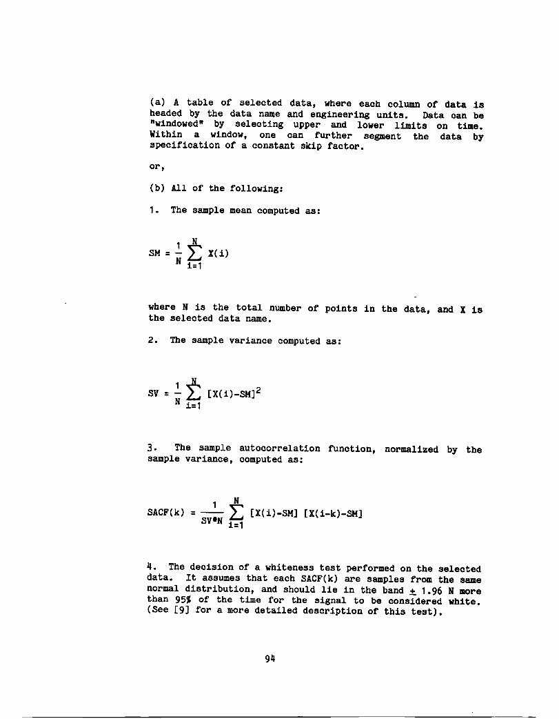
(a) A table of selected data, where each column of data is headed by the data name and engineering units. Data can be "windowed" by selecting upper and lower limits on time. Within a window, one can further segment the data by specification of a constant skip factor.

or,

(b) All of the following:

1. The sample mean computed as:

SM = ..!. t XCi) N i=1

where N is the total number of pOints in the data, and X is the selected data name.

2. Tbe sample variance computed as:

SV = ..!. t [X(i)-SM]2 N i=1

3. The sample autocorrelation function, normalized by the sample variance, computed as:

1 N SACF(k) = -- ~ [X(i)-SM] [X(i-k)-SM]

SV*N i=1

4. The decision of a whiteness test performed on the selected data. It assumes that each SACF(k) are samples from the same normal distribution, and should lie in the band ± 1.96 N more than 95% of the time for the signal to be cons1dered wh1 te. (See [9] for a more detailed description of this test).

94

A.2 Desoription ot Program: PLOro

Purpose:

Operation:

Outputs:

To plot the unformatted (binary) time history data stored in the .PLT file generated by FINDS.

To invoke PLOTD, the user simply types (at the monitor level):

$ ROlf PLOro

PLOTD will then prompt the user for various directive commands. Time history data is identified by a unique name saved in the .PLT file. (See Table 6 on page 82 for a list of these names).

PLOTD can be used to generate plots of one, or several variables versus time, or to create cross plots of one variable vs. another. Currently, PLOTD creates a Single plot/page. The plots can be drawn on any of the following devices or saved in a device independent disk file: TEKTRONIX 4010 or 4014, and RETROGRAPHICS.

95

This Page Intentionally Left Blank

6. RBFBRDCBS

[1] "An Aircraft Sensor Fault Tolerant System", A.K. Caglayan and R.E. Lancraft, NASA CR-165876, April 1982.

[2] "A Fault Tolerant System for an Integrated Avionics Sensor Configuration", A.K. Caglayan and R.E. Lancraft, BBN Report No. 5352, Bolt Beranek and Newman, Inc., Cambridge, HA, October 1983.

[3] "Terminal Area Automatic Navigation, Guidance and Control Research Using the Microwave Landing System (HLS), Part 2 - RNAY/HLS Transition Problems for Aircraft", S. Pines, NASA CR-3511, January 1982.

[4] "Terminal Area Automatic Navigation, Guidance and Control Research USing the Microwave Landing System (HLS, Part 3 - A Comparison of Waypoint Guidance Algorithms for RNAY/HLS TranSitions", S. Pines, NASA CR-3512, January 1982.

[5] "Automated Landing, Rollout, and Turnoff Using HLS and Magnetic Cable Sensors", S. Pines, S.F. SChmidt, and F. Mann, NASA CR-2907, October 1977.

[6] "Design of a Developmental Dual Fail Operational Redundant Strapped Down Inertial Measurem~nt Unit", F.R. Morrell and J.G. Russell, NAECON, May 1980.

[7] "YAX-11 FORTRAN Language Reference Manual. (YMS Y3.0)", Digital Equipment Corporation, 1982

[8] Preliminary Design of a Redundant Strapped Down Inertial Navigation Unit USing Two-Degree-of-Freedom Tuned-Gimbal Gyroscopes", Litton Guidance and Control Systems, NASA CR-145035, October 1976.

[9] "An Innovations Approach to Fault Detection and Diagnosis in Dynamic Systems", R.K. Mehra and J. Peschon, Automatica, Vol. 7, 1971.

[10] "Failure Detection and Isolation Analysis of a Redundant Strapdown Inertial Measurement Unit", P. Motyka, M. Landey, and R. McKern, NASA CR-165658, February 1981.

[11] "Wind Models for Flight Simulator Certification of Landing and Approach Guidance and Control Systems", N.M. Barr, D. Gangaas and D.R. Schaeffer, FAA­RD-74-206, December 1974.

97

This Page Intentionally Left Blank

IBDU

FILTER 18 GUST 21 AC 45 FILTIN 57, 60 ACSTAT 56, 58 FIN 25 HG 23 AG 25 FINAG 43 HIGHT 20 AIRSPE 20 FINAR 51 HRADAR 55 ANGBND 55 FINAS 37 AR 25 FINGR 48 IC 24 AS 25 FINLA 41 ICNTRL 53, 73

FINHL 46 ID 25 BOUNAZ 45 FINRA 36 IDAG 43 BOUNEL 45 FINRG 39 IDAR 50 BOUNRN 45 FP 25 IDAS 36 BTHRSH 55 FPAG 57, 59 IDGR 47

FPAR 57, 60 IDLA 40 CA 46 FPAS 56, 58 IDML 45 CG 20 FPGR 57, 59 IDRA 35 CPUCHK 19 FPLA 57, 59 IDRG 38

FPHL 57 lEST 19, 73 DT 25 FPHLS 59 IGUST 21 DTAG 43 FPRA 56, 58 lHEAD 19 DTAR 50 FPRG 56, 59 IIHUF 53, 73 DTAS 37 FR 25 INOBPS 53 DTGR 47 FRAG 44 IPARGR 49 DTlME 18 FRAR 51 IPFOAR 52 DTLA 41 FRAS 37 IPFOGR 49 DTHL 45 FRGR 49 IPRNT 19 DTRA 35 FRLA 42 IREP 25 DTRG 38 FRHL 46 IREPAG 43

FRRA 36 IREPAS 37 FDI 25 FRRG 40 IREPLA 41 FDIAR 57, 60 FSF 25 IREPHL 45 FDIGR 57, 59 FSFAR 51 IREPRA 35 FIB 25 FSFGR 49 IREPRG 38 FIBAG 44 FSFLA 42 IRSDF 53, 73 FIBAR 51 FSFRG 40 IRSDFY 53 FIBAS 37 FTHRSH 55 IRSOIH 47 FIBGR 49 IWHHLS 45 FIBLA 42 GPIPRN 21 FIBHL 46 GR 25 KHXEWH 53 FIBRA 36 GRQSF 48 KHXHLR 53 FIBRG 39 GSLOC 56, 58 KPATH 23

99

KPRINT 19 QDEG 20 SHEAR 21 SHZ 23

LA 25 RA 25 SIG 54 LOCRAN 21 RDEG 20 SLA 23

RE 20 SLIM 25 HI. 25 RG 25 SLIMAG 43 MP 25 RHO 20 SLlMAR 50 MPAG 51, 59 RINLA 20 SLlMAS 31 MPAR 51, 59 RINLO 20 SLIMGR 48 MPAS 56, 58 ROLL 20 SLIMLA 41 MPGR 51, 59 RT 23 SLIMRA 35 MPLA 56, 59 SLIMRG 39 MPMLS 51, 59 SCALEW 21 SLO 23 MPRA 56, 58 SDB 25 SNDP 24 MPRG 56, 58 SDBAG 43 STARTER 56, 58

SDBAR 50 NDISTB 0 SDBAS 31 TANLIM 24 NEWPTH 23 SDBGR 41 TF 25 NFMAX 0 SDBLA 41 TFAG 44 NFT 0 SDBML 45 TFAR 51 NTICK 19 SDBRA 35 TFAS 38 NUl 0 SDBRG 38 TFGR 49 NW 23 SDGDGR 48 TFLA 42 NX 0 SDMN 25 TFML 46 NYMAX 0 SDMNAS 31 TFRA 36

SDN 25 TFRG 40 OUTPS 19 SDNAG 43 THETAG 22

SDNAR 50 THRUST 20 PBFOI 54 SDNGR 41 TSTOP 19 PBFIC 54 SDNLA 41 PDEG 20 SDNML 45 VELBND 54 PFKAR 52 SDNRA 35 VGD 23 PFKGR 49 SDNRG 38 PFTCAR 52 SDPIC 54 WEIGHT 20 PFTCGR 49 SDSF 25 WINDAT 56, 58 PFTHAR 52 SDSFAR 50 WINDOW 53 PFTHGR 49 SDSFGR 48 WINDSS 21 PITCH 20 SDSFLA 41 WLA 23 PLOTS 19 SDSFRG 39 WLO 23 POSBND 54 SDSUBW 21 PRIORI 54 SDTM 25 XAZ 45 PRIORJ 54 SDTMGR 48 XEL 45 PRNTPL 56, 58 SDTMLA 41 PROGCN 18, 56, 58 SDTHRG 39 YAW 20 PSIR 22 SDXIC 54 YSTOP 19 PSIW 21 SH1 21

SH2 21

100

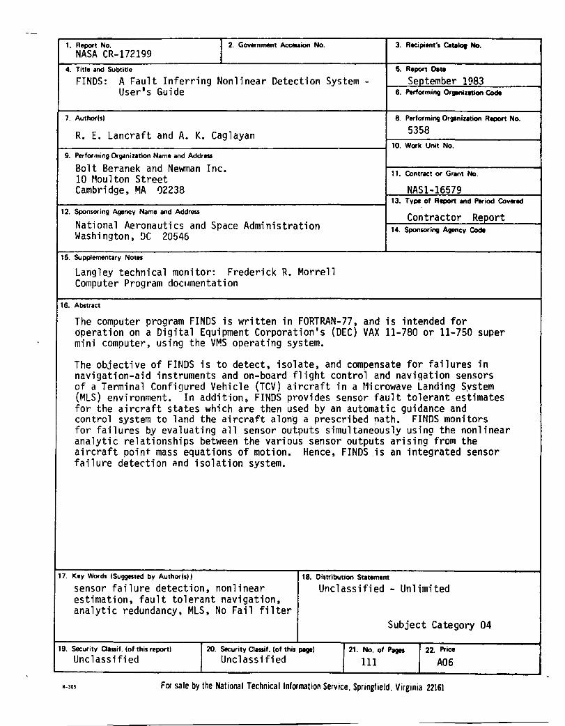
1. Report No. NASA CR-I72199

I 2. Government Ace_ion No. 3. Recipient's c.talot No.

4. Title and Subtitle 5. Report Dlt.

FINDS: A Fault Inferring Nonlinear Detection System -User1s Guide

September 1983 6. Performing Orglnizltion Code

7. Authorls) 8. Performing Organizltion Report No.

R. E. Lancraft and A. K. Caglayan 5358 ...-----------------------------i 10. Work Unit No.

9. Performing Organization Name and Address

Bolt Beranek and Newman Inc. 10 Moulton Street Cambridge, MA 02238

11. Contract or Gr.nt No.

NASI-16579 1-----------------------------4 13. Type of Report and Period Covered

12. Sponsoring Agency Name and Address

National Aeronautics and Space Administration Washington, nc 20546

15. Supplementary Notes

Langley technical monitor: Frederick R. Morrell Computer Program documentation

16. Abstract

Contractor Report 14. Sponsoring Agency Code

The computer program FINDS is written in FORTRAN-77, and is intended for operation on a Digital Equipment Corporation's (DEC) VAX 11-780 or 11-750 super mini computer, using the VMS operating system.

The objective of FINDS is to detect, isolate, and compensate for failures in navigation-aid instruments and on-board flight control and naviqation sensors of a Terminal Configured Vehicle (TCV) aircraft in a t1icrowave Landing System (MLS) environment. In addition, FINDS provides sensor fault tolerant estimates for the aircraft states which are then used by an automatic guidance and control system to land the aircraft along a prescribed !"lath. FINDS monitors for failures by evaluating all sensor outputs simultaneously using the nonlinear analytic relationships between the various sensor outputs arising from the aircraft point mass equations of motion. Hence, FINDS is an integrated sensor failure detection ~nd isolation system.

17. Key Words ISuggested by Authorls)) 18. Oistribution Stltement

sensor failure detection, nonlinear Unclassified - Unlimited estimation, fault tolerant navigation, analytic redundancy, MLS, No Fail filter

19. Security C'S1if. lof this report)

Unclassified 20. Security a.ssif. lof this page)

Unclassified

Subject Category 04

21. No. of Pages

111 22. Price

A06

N-305 For sale by the National Technical Information Service, Springfield. Virginia 22161

End of Document