NuCAD ACG - Adjacent Constraint Graph

for General Floorplans

Hai Zhou and Jia Wang

ICCD 2004, San JoseOctober 11-13, 2004

(2)

Outline

• Floorplan and Constraint Graph

• Adjacent Constraint Graph

• Data Structure and Operations

• Experimental Result

• Summary

(3)

Floorplan

• A floorplan contains non-overlapping modules.

a

bd

c

e

(4)

Constraint Graph

• Horizontal graph represents “left to” relation.

a

b

d

ce

(5)

Constraint Graph

• Vertical graph represents “below” relation.

a

b d

ce

(6)

Constraint Graph

• There is at least one relation between any pair of modules.

a

b

d

ce

(7)

a

b

d

ce

Redundancy in constraint graphs.

• Transitive edges.

(8)

a

b

d

ce

Redundancy in constraint graphs.

• Over-specification: more than one relation between two modules.

(9)

Reduce the redundancy.

• Less edges means less running time and less storage requirement.

• Allow exactly one relation between any pair of modules.

• Remove all the transitive edges.

• Combine horizontal graph and vertical graph together. Two types of edges: H and V.

The remaining edges form a total order!

b a d c e

(10)

Cross

• There are totally O(n2) edges in the two constraint graphs where n is the number of modules.

• Can we get rid of that quadratic boundary by the previous steps?

V H H

H V V

• No. In the graph to the right, we have more than k2 edges where there are only 2k modules.

1

2 k+2

k+1

... ...

... k+2 ...

k k+2 2k• The basic structure could be identified as crosses in the graph.

a b c d

a b c d

(11)

ACG-Adjacent Constraint Graph

• Definitions of ACG Constraint graph.

Exactly one relation between every pair of modules.

No transitive edges.

No cross.

b a d c e

a b c d a c b d

• Observation: in VHH cross, either ‘a’ is below ‘d’ or ‘c’ is below ‘b’. Has similar result for HVV cross.

(12)

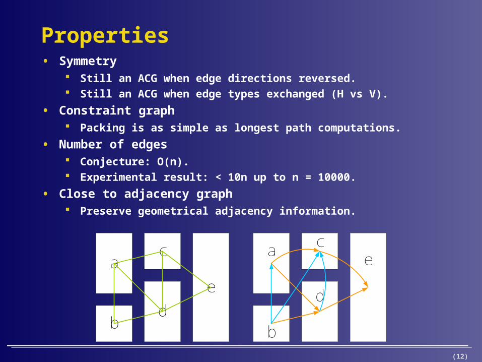
Properties• Symmetry

Still an ACG when edge directions reversed. Still an ACG when edge types exchanged (H vs V).

• Constraint graph Packing is as simple as longest path computations.

• Number of edges Conjecture: O(n). Experimental result: < 10n up to n = 10000.

• Close to adjacency graph Preserve geometrical adjacency information.

a

bd

c

e

a

b

d

ce

(13)

Data structure

• Vertices representing modules are linked as the total order.

• Every vertex maintains 4 lists of edges. Correspond to 4 geometrical relationships (left/right, below/above).

• Every edge keeps its two end vertices.

• Every edge belongs to 2 lists (incoming/outgoing). Edges from one list have a common end vertex. An edge with a closer end vertex to the common vertex comes first.

b a d c e

(14)

Operations

• Guideline Maintain a valid ACG through operations to control the n

umber of edges.

Operation cost (time/space) should be linear to the edges added/deleted.

• Append We could construct an ACG by appending vertices.

• Swap Will introduce crosses into the graph.

Swapping is complete when we allow crosses in ACG.

(15)

new a b c

Append

• Step 1: add edges with the same type. Always follow the first edge of the other type to determine the

next new edge.

new a b c d

• Step 2: add the first edge of the other type. Still follow the first edge of the other type.

(16)

new a b c d e f

Append

• Step 3: add edges whose types alternating. Follow the edge after the edge connecting the other end points

of the two previous added edges.

• Stop when we cannot proceed with step 3.

(17)

Swap

• Step 1: exchange the positions of the two vertices. This won’t affect the edge lists. Suppose we are going to swap b and c.

a b c d e

• Step 2: change the edge type. Need to change the edge direction too, i.e., from b->c to c->b.

a bc d e

(18)

Swap

• Step 3: remove transitive edges. Check c’s outgoing V neighbors and b’s incoming V neighbors.

a bc d e

(19)

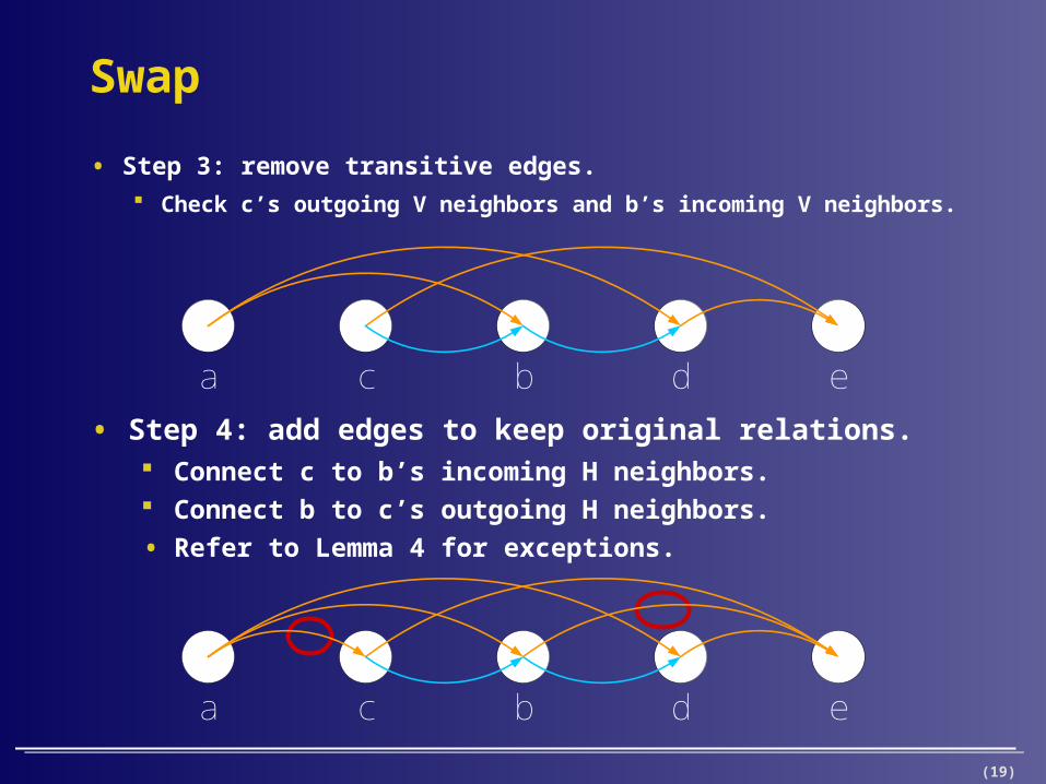
Swap

• Step 3: remove transitive edges. Check c’s outgoing V neighbors and b’s incoming V neighbors.

a bc d e

• Step 4: add edges to keep original relations. Connect c to b’s incoming H neighbors. Connect b to c’s outgoing H neighbors.

• Refer to Lemma 4 for exceptions.

a bc d e

(20)

Experiment Setup

• MCNC benchmarks: apte, hp, xerox, ami33, ami49.

• GSRC benchmarks: n100, n200, n300.

• Create ACG with appending operations.

• Employ the simulated annealing algorithm. Adopt an annealing scheme similar to TCG-S.

Perturbations• Change the orientation of a module.

• Exchange two modules.

• Swapping two adjacent vertices.

Allow crosses in ACG during perturbations.

• Compare running time as well as solution quality to FAST-SP, TCG, TCG-S, and Parquet-2 on area optimization.

• Running on a Sun Ultra 10, running time is in seconds.

(21)

Experimental Result• Compare to FAST-SP, TCG, and TCG-S on all the benchmarks.

• Compare to Parquet-2 on the GSRC benchmarks.

• We cut the number of perturbations by half in our SA.

(22)

Experimental Result (Cont.)

• Number of edges. Min/max edge give the

minimal/maximal number of edges in the graph during SA.

Even we allow crosses, the number keeps small during SA.

• Floorplan for xerox with ACG edges. Most edges are

between adjacent modules.

(23)

Summary

• ACG is a constraint graph.

• ACG is like an adjacency graph due to the fact that the redundancies in the traditional H/V constraint graphs are reduced.

• We have a neat data structure plus efficient operations.

• Future directions. Enforce the no-cross rule in operations. Interconnect estimation and planning (ASP-DAC 2005). Is the number of edges really O(n)?

(24)

Thanks!