null geodesics of the kerr exterior · null geodesics of the kerr exterior samuel e. gralla1, and...
TRANSCRIPT
Null Geodesics of the Kerr Exterior
Samuel E. Gralla1, ∗ and Alexandru Lupsasca2, 3, †
1Department of Physics, University of Arizona, Tucson, Arizona 85721, USA2Center for the Fundamental Laws of Nature, Harvard University, Cambridge, Massachusetts 02138, USA
3Society of Fellows, Harvard University, Cambridge, Massachusetts 02138, USA
The null geodesic equation in the Kerr spacetime can be expressed as a set of integral equationsinvolving certain potentials. We classify the roots of these potentials and express the integrals inmanifestly real Legendre elliptic form. We then solve the equations using Jacobi elliptic functions,providing the complete set of null geodesics of the Kerr exterior as explicit parameterized curves.
I. INTRODUCTION
Null geodesics form perhaps the most important struc-ture possessed by a Lorentzian spacetime. The study ofthe null geodesic equation in the Kerr geometry beganin 1968 with the seminal work of Carter [1], who usedthe separability of its Hamilton-Jacobi formulation to re-duce it to quadratures. Bardeen [2] initiated the detailedstudy of its solution space, which has now been mappedout in impressive detail [3–5]. Many of the relevant inte-grals have previously been expressed in elliptic form (no-tably in Refs. [6–8]), and parameterized solutions usingthe Weierstrass elliptic function were given in Ref. [5].
In this paper, we revisit the problem of the classifica-tion and solution of Kerr null geodesics with the goals ofcompleteness and convenience. Our results are completein that every finite-measure case is considered, and wegive both “integral solutions” (analytic expressions forthe fundamental integrals) as well as explicit parameter-ized trajectories.1 Moreover, our results are convenient inthat: (1) all expressions are manifestly real, with no “can-celing” internal imaginary parts; (2) all trajectories arefully explicit, with no need to solve auxiliary equationsor glue together different solutions at turning points; (3)the parameterized solutions display the initial conditionsexplicitly; and (4) the use of special functions is limitedto the elliptic integrals and Jacobi elliptic functions firstdefined two centuries ago. While previous approachesachieve one or more of these goals, we are unaware ofany previous work that simultaneously attains them all.
Our own interest in this problem was kindled by theneed to understand astronomical observations [9], but wehope that the results presented herein will find a widerrange of applications. Ideally, the Kerr afficionado willlearn something about the general structure of the nullgeodesics, while the busy physicist or astronomer can ob-tain quick answers to definite questions about the prop-agation of light around a rotating black hole.
This paper is organized as follows. In Sec. II, we in-troduce the basic formulas and explain our general ap-proach. In Sec. III, we classify and solve for the different
∗ [email protected]† [email protected]
1We do limit our discussion to the Kerr exterior, however.
types of polar motion, before doing the same for the ra-dial motion in Sec. IV and App. B. We then compare toprevious work in Sec. V. Finally, in Sec. VI, we summa-rize our results and explain how to use them in practice.
II. GENERAL APPROACH
We work with Boyer-Lindquist coordinates (t, r, θ, φ)on the spacetime of a Kerr black hole with mass M andangular momentum J = Ma, and define
Σ(r, θ) = r2 + a2 cos2 θ, ∆(r) = r2 − 2Mr + a2. (1)
The roots of ∆(r) correspond to the outer/inner horizons
r± = M ±√M2 − a2. (2)
We assume 0 < a < M throughout the paper. Takingthe nonrotating limit a→ 0 is generally straightforward,whereas the extremal limit a → M presents some sub-tleties that we defer to future work.
Let pµ denote the four-momentum of a photon, withpt > 0 providing the time orientation. The trajectorypossesses three conserved quantities,
E = −pt, L = pφ, (3)
Q = p2θ − cos2 θ(a2p2t − p2φ csc2 θ
), (4)
corresponding to the energy at infinity,2 angular momen-tum about the spin axis, and Carter integral, respec-tively. Only the sign of the energy has physical meaning,so it is convenient to work with energy-rescaled quantities
λ =L
E, η =
Q
E2. (5)
The four-momentum pµ can then be reconstructed as
Σ
Epr = ±r
√R(r), (6a)
Σ
Epθ = ±θ
√Θ(θ), (6b)
Σ
Epφ =
a
∆
(r2 + a2 − aλ
)+
λ
sin2 θ− a, (6c)
Σ
Ept =
r2 + a2
∆
(r2 + a2 − aλ
)+ a(λ− a sin2 θ
), (6d)
2We exclude the measure-zero set of geodesics with E = 0 exactly.
arX
iv:1
910.
1288
1v3
[gr
-qc]
20
Jul 2
020
2
where we introduced “potentials”
R(r) =(r2 + a2 − aλ
)2 −∆(r)[η + (λ− a)
2], (7)
Θ(θ) = η + a2 cos2 θ − λ2 cot2 θ. (8)
The symbols ±r and ±θ indicate the sign of pr and pθ,respectively. Turning points in the r and θ motions occurat zeros of the radial and angular potentials R(r) andΘ(θ), respectively.
There are two closely related ways to proceed with thesolution of these equations. The first is to introduce anew parameter, the “Mino time” τ [10], defined by3
dxµ
dτ=
Σ
Epµ. (9)
This method converts Eqs. (6) into four decoupled ordi-nary differential equations for xµ(τ). Alternatively, onemay also convert the equations into integral form,
Ir = Gθ, (10)
φo − φs = Iφ + λGφ, (11)
to − ts = It + a2Gt, (12)
where xµs and xµo are “source” and “observer” points, φcan take any real value (with b(φo−φs)/(2π)c the numberof azimuthal windings of the trajectory), and we define
Ir =
ro
rs
dr
±r√R(r)
, (13a)
Iφ =
ro
rs
a(2Mr − aλ)
±r∆(r)√R(r)
dr, (13b)
It =
ro
rs
r2∆(r) + 2Mr(r2 + a2 − aλ
)
±r∆(r)√R(r)
dr, (13c)
Gθ =
θo
θs
dθ
±θ√
Θ(θ), (13d)
Gφ =
θo
θs
csc2 θ
±θ√
Θ(θ)dθ, (13e)
Gt =
θo
θs
cos2 θ
±θ√
Θ(θ)dθ. (13f)
Here, the slash notationffl
indicates that these integralsare to be understood as path integrals along the trajec-tory connecting xµs and xµo , such that the signs ±r and ±θswitch at radial and angular turning points, respectively.In particular, all the integrals Ii and Gi are monotoni-cally increasing along the trajectory.
These two approaches are related by the fact that Irand Gθ are both equal to the elapsed Mino time,4
τ = Ir = Gθ, (14)
3The geodesic xµ(τ) is future/past-directed according to whetherE is positive/negative. Sending τ → −τ reverses the future/pastdirection of the parameterized curve xµ(τ).
4τ is also related to the fractional number of orbits executed [11].
where we set τ = 0 at the source point xµs . The Mino timeapproach is more convenient for analyzing individual tra-jectories, while the integral approach is more useful fordetermining general properties.
The elapsed affine time (satisfying dxµ/dσ = pµ) is
σo − σs = Iσ + a2Gt, (15)
where
Iσ =
ro
rs
r2
±r√R(r)
dr. (16)
Our main results are as follows. First, we systemati-cally classify the roots of the radial and angular poten-tials, and thereby determine the allowed ranges of the rand θ motion as a function of the conserved quantities(λ, η). Then, for each of the cases that may arise, andfor each integral Ii or Gi, we find an antiderivative thatis real and smooth over the relevant range of r or θ. Allof our antiderivatives are reduced to manifestly real Leg-endre elliptic form. That is, they are expressed in termsof the (incomplete) elliptic integrals F (ϕ|k), E(ϕ|k), andΠ(n;ϕ|k) of the first, second, and third kind, respectively,which are real and smooth provided max(k, n) < 1.5
When ϕ = π/2, the integrals become “complete” andare denoted by K(k) = F (π/2|k), or else by Π(n; k) andE(k) with the first argument ϕ omitted.
Our notation for antiderivatives will be a calligraphicversion of the original symbol, and we will choose the plussign in the integrand. For example, the antiderivative Irassociated with Ir in Eq. (13a) will satisfy
dIrdr
=1√R(r)
. (17)
These antiderivatives are useful for both the Mino-timeapproach and the integral approach. For the Mino-timeapproach, we invert the integrals to provide full parame-terized trajectories xµ(τ) in terms of the initial data (ini-tial position xµs as well as the initial signs ±r and ±θ).6For the integral approach, we provide formulas that giveeach of the path integrals (13) as a function of the initialposition, initial sign of momentum, final position, andnumber of turning points.
III. ANGULAR POTENTIAL AND INTEGRALS
We assume that 0 < θ < π to avoid the singularities ofthe spherical coordinate system. In terms of u = cos2 θ,the angular potential (8) is given by
(1− u)Θ(u) = η +(a2 − η − λ2
)u− a2u2. (18)
5Our conventions are listed in App. A of Ref. [8]; these also matchthe built-in implementation in Mathematica 12.
6The full initial derivative can then be reconstructed from Eqs. (6),showing how this initial value problem is equivalent to the originalsecond-order initial value problem for the geodesic equation.
3
The right-hand side is a quadratic polynomial, whoseroots u± are given by
u± = 4θ ±√42θ +
η
a2, 4θ =
1
2
(1− η + λ2
a2
). (19)
The four roots of Θ(θ) are thus arccos(±√u±
), or
θ1 = arccos(√u+), (20)
θ2 = arccos(√u−), (21)
θ3 = arccos(−√u−
), (22)
θ4 = arccos(−√u+
). (23)
Roots coincide when (and only when) u+ = 0, u− = 0,or u+ = u−. These conditions define curves throughthe (λ, η)-plane that divide it up into several regions. Ineach such region, the “character” of the potential—thatis, the number of real roots and the sign of the potentialon either side of them—cannot change. As such, we maydetermine the character by evaluating a single point ineach region.
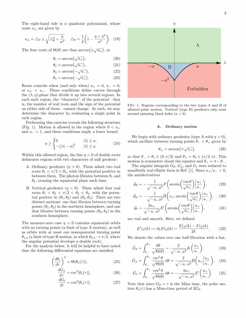
Performing this exercise reveals the following structure(Fig. 1). Motion is allowed in the region where 0 < u+and u− < 1, and these conditions imply a lower bound
η ≥{
0 |λ| ≥ a,−(|λ| − a)
2 |λ| ≤ a. (24)
Within this allowed region, the line η = 0 of double rootsdelineates regions with two characters of null geodesic:
A. Ordinary geodesics (η > 0). These admit two realroots θ1 < π/2 < θ4, with the potential positive inbetween them. The photon librates between θ1 andθ4, crossing the equatorial plane each time.
B. Vortical geodesics (η < 0). These admit four realroots θ1 < θ2 < π/2 < θ3 < θ4, with the poten-tial positive in (θ1, θ2) and (θ3, θ4). There are twodistinct motions: one that librates between turningpoints (θ1, θ2) in the northern hemisphere, and onethat librates between turning points (θ3, θ4) in thesouthern hemisphere.
The measure-zero case η = 0 contains equatorial orbitswith no turning points (a limit of type A motion), as wellas orbits with at most one nonequatorial turning pointθ1,4 (a limit of type B motion, in which θ2,3 → π/2, wherethe angular potential develops a double root).
For the analysis below, it will be helpful to have notedthat the following differential equations are satisfied:
(dθodτ
)2
= Θ(θo(τ)), (25)
dGφdτ
= csc2[θo(τ)], (26)
dGtdτ
= cos2[θo(τ)]. (27)
FIG. 1. Regions corresponding to the two types A and B ofallowed polar motion. Vortical (type B) geodesics only existaround spinning black holes (a > 0).
A. Ordinary motion
We begin with ordinary geodesics (type A with η > 0),which oscillate between turning points θ− < θ+ given by
θ± = arccos(∓√u+
), (28)
so that θ− = θ1 ∈ (0, π/2) and θ+ = θ4 ∈ (π/2, π). Thismotion is symmetric about the equator and θ+ = π−θ−.
The angular integrals Gθ, Gφ, and Gt were reduced tomanifestly real elliptic form in Ref. [8]. Since u+/u− < 0,the antiderivatives
Gθ = − 1√−u−a2
F
(arcsin
(cos θ√u+
)∣∣∣∣u+u−
), (29)
Gφ = − 1√−u−a2
Π
(u+; arcsin
(cos θ√u+
)∣∣∣∣u+u−
), (30)
Gt =2u+√−u−a2
E′(
arcsin
(cos θ√u+
)∣∣∣∣u+u−
), (31)
are real and smooth. Here, we defined
E′(ϕ|k) := ∂kE(ϕ|k) =E(ϕ|k)− F (ϕ|k)
2k. (32)
We denote the values over one half-libration with a hat,
Gθ =
ˆ θ+
θ−
dθ√Θ(θ)
=2√−u−a2
K
(u+u−
), (33)
Gφ =
ˆ θ+
θ−
csc2 θ√Θ(θ)
dθ =2√−u−a2
Π
(u+
∣∣∣∣u+u−
), (34)
Gt =
ˆ θ+
θ−
cos2 θ√Θ(θ)
dθ = − 4u+√−u−a2
E′(u+u−
). (35)
Note that since Gθ = τ is the Mino time, the polar mo-tion θo(τ) has a Mino-time period of 2Gθ.
4
1. Inversion for θo(τ)
Now consider the path integral Gθ = τ beginning fromθ = θs. Before the first turning point is reached, we have
τ = Gθ = νθ(Goθ − Gsθ), νθ = sign(pθs), (36)
where Giθ indicates the antiderivative Gθ evaluated at thesource (i = s) or observer (i = o). This equation can beinverted for θo using the Jacobi elliptic sine function,
sn(F (arcsinϕ|k)) = ϕ, (37)
which is odd in its first argument, sn(−ϕ|k) = − sn(ϕ|k).Combining Eqs. (29), (36), and (37) therefore gives
cos θo√u+
= −νθ sn
(√−u−a2(τ + νθGsθ)
∣∣∣∣u+u−
). (38)
Although Eq. (38) was derived under the assumption thata turning point has not yet been reached, it in fact con-tinues properly through turning points to provide the fullparameterized trajectory θo(τ), as follows. Noting thatsn(ϕ|k) oscillates smoothly between −1 and +1 with half-period 2K(k), we see that Eq. (38) defines a trajectoryθo(τ) that oscillates between θ− and θ+ with half-period
Gθ. Thus, it has the correct quantitative behavior atturning points, and we need only check that it satisfiesthe squared differential equation (25), which is easily ver-ified using the elliptic identities [12]
cn2(ϕ|k) + sn2(ϕ|k) = 1, (39)
dn2(ϕ|k) + k sn2(ϕ|k) = 1. (40)
This completes the proof that Eq. (38) is the unique so-lution for θo(τ) with initial conditions θo(0) = θs andsign[θ′o(0)] = νθ.
2. Path integrals as functions of Mino time
We have Gθ = τ by definition, and the other pathintegrals may be expressed in terms of Mino time τ asfollows. Before a turning point is reached, we have
Gφ = νθ(Goφ − Gsφ
), (41)
Gt = νθ(Got − Gst ). (42)
To manipulate these equations, we will invoke a secondinversion formula,
am(ϕ|k) = arcsin(sn(ϕ|k)), |ϕ| ≤ K(k). (43)
where the Jacobi amplitude am(ϕ|k) is defined as theinverse of the elliptic integral of the first kind F (ϕ|k),
F (am(ϕ|k)|k) = ϕ. (44)
Applying the formula (43) to Eq. (38) yields
arcsin
(cos θo√u+
)= −νθΨτ , (45)
where the (monotonically increasing in τ) amplitude is
Ψτ = am
(√−u−a2(τ + νθGsθ)
∣∣∣∣u+u−
), (46)
and the restriction |ϕ| ≤ K(k) is satisfied on account ofour assumption that a turning point has not yet beenreached. Plugging Eq. (45) into Eqs. (41) and (42) asneeded, and noting that both Π(n;−ϕ|k) = −Π(n;ϕ|k)and E′(−ϕ|k) = −E′(ϕ|k) are odd in ϕ, we then find
Gφ =1√−u−a2
Π
(u+; Ψτ
∣∣∣∣u+u−
)− νθGsφ, (47)
Gt = − 2u+√−u−a2
E′(
Ψτ
∣∣∣∣u+u−
)− νθGst . (48)
Although Eqs. (47) and (48) were derived under the as-sumption that a turning point does not occur, they infact extend properly through turning points to give thecomplete path integrals Gφ and Gt, as follows. Sinceam(ϕ|k), Π(n;ϕ|k) and E′(ϕ|k) are real and smoothfunctions of ϕ provided max(k, n) < 1 (satisfied here fork = u+/u− and n = u+), it follows that the candidateformulas for Gφ and Gt are real and smooth. Thus, weneed only check the differential equations (26) and (27),which is straightforward using the identity (40). Thiscompletes the proof that Eqs. (47) and (48) give the fullpath integrals (13e) and (13f).
Notice that Eq. (38) may also be put in a similar formusing sn(ϕ|k) = sin(am(ϕ|k)),
cos θo(τ) = −νθ√u+ sin Ψτ . (49)
3. Path integrals in terms of turning points
Finally, it is useful for some purposes to express thepath integrals Gi as functions of θs, θo, νθ, and the num-ber of turning points m encountered along the trajectory.A general treatment is given in App. A below. For type Amotion, the antiderivatives Gi are odd under interchangeof + and −,
G+i = −G−i , (50)
where the ± denotes evaluation of Gi at θ = θ±. Thisproperty originates from the equatorial reflection sym-metry Θ(θ) = Θ(π − θ) of the angular potential. Thegeneral result (A10) therefore reduces to
Gi = mGi + νθ[(−1)mGoi − Gsi ], (51)
for i ∈ {θ, φ, t}, in agreement with Eqs. (80) in Ref. [8].

5
It is instructive to examine the relationship betweenthis formula and the above expressions parameterized byMino time. When i = θ, Eq. (51) is the Mino time itself,
τ = mGθ + νθ[(−1)mGoθ − Gsθ ]. (52)
By using the quasiperiodicity properties
am(ϕ+ 2K(k)|k) = am(ϕ|k) + π, k < 1, (53a)
F (ϕ+ π|k) = F (ϕ|k) + 2K(k), (53b)
Π(n;ϕ+ π|k) = Π(n;ϕ|k) + 2Π(n; k), (53c)
E(ϕ+ π|k) = E(ϕ|k) + 2E(k), (53d)
one can plug Eq. (52) into Eqs. (47), (48), and (49) torecover Eq. (51) for i ∈ {φ, t}, and verify that θo(τ) = θo,as required for consistency.
B. Vortical motion
We next turn to vortical geodesics (type B with η < 0),which oscillate within a single hemisphere determined by
h = sign(cos θ). (54)
The motion lies within a cone θ− < θ+ in the north-ern hemisphere (h = +1), or θ+ < θ− in the southernhemisphere (h = −1), with the turning points given by
θ± = arccos(h√u∓), (55)
so that θ−,+ = θ1,2 for h = 1 and θ+,− = θ3,4 for h = −1.The angular integrals Gθ, Gφ, and Gt were reduced to
manifestly real elliptic form in Ref. [8]. Since u+/u− > 0,the antiderivatives
Gθ = − h√u−a2
F
(Υ
∣∣∣∣1−u+u−
), (56)
Gφ = − h
(1− u−)√u−a2
Π
(u+ − u−1− u−
; Υ
∣∣∣∣1−u+u−
), (57)
Gt = −h√u−a2E
(Υ
∣∣∣∣1−u+u−
), (58)
are real and smooth, with
Υ = arcsin
√cos2 θ − u−u+ − u−
. (59)
Their values over one half-libration are
Gθ = h
ˆ θ+
θ−
dθ√Θ(θ)
=1√u−a2
K
(1− u+
u−
), (60)
Gφ = h
ˆ θ+
θ−
csc2 θ√Θ(θ)
dθ
=1
(1− u−)√u−a2
Π
(u+ − u−1− u−
; 1− u+u−
), (61)
Gt = h
ˆ θ+
θ−
cos2 θ√Θ(θ)
dθ =
√u−a2E
(1− u+
u−
), (62)
and Gθ once again denotes the Mino-time half-period ofthe polar motion θo(τ).
1. Inversion for θo(τ)
Now consider the path integral Gθ = τ beginning fromθ = θs. Before the first turning point is reached, we onceagain have Eq. (36), which can yet again be invertedusing Eq. (37) to obtain
√cos2 θo − u−u+ − u−
= −hνθ sn
(√u−a2(τ + νθGsθ)
∣∣∣∣1−u+u−
).
(63)
Solving for cos θo and using the identity (40) yields
cos θo√u−
= hdn
(√u−a2(τ + νθGsθ)
∣∣∣∣1−u+u−
), (64)
where in taking the square root, we chose the branchh = ±1 to obtain the motion in the correct hemispherevia Eq. (54). Although Eq. (64) was derived under the as-sumption that a turning point has not yet been reached,it in fact continues properly past turning points to pro-vide the full parameterized trajectory θo(τ), as before.Noting that when k < 0, dn(ϕ|k) oscillates smoothly be-tween +1 and +
√1− k with period 2K(k), we see that
Eq. (64) defines a trajectory θo(τ) that oscillates between
θ− and θ+ with half-period Gθ. Thus, it has the correctquantitative behavior at turning points, and we need onlycheck that it satisfies the squared differential equation(25) is satisfied, which is easily verified using the ellip-tic identities (39) and (40). This completes the proofthat Eq. (64) is the unique solution for θo(τ) with initialconditions θo(0) = θs and sign[θ′o(0)] = νθ.
2. Path integrals as functions of Mino time
We have Gθ = τ by definition, and the other pathintegrals may be expressed in terms of Mino time τ bythe same method as in the ordinary case above. Beforea turning point is reached, we once again have Eqs. (41)and (42). Applying the formula (43) to Eq. (63) yields
arcsin
√cos2 θo − u−u+ − u−
= −hνθΥτ , (65)
where the (monotonically increasing in τ) amplitude is
Υτ = am
(√u−a2(τ + νθGsθ)
∣∣∣∣1−u+u−
), (66)
and the restriction |ϕ| ≤ K(k) is satisfied on account ofour assumption that a turning point has not yet beenreached. Plugging Eq. (65) into Eqs. (41) and (42) asneeded, and recalling that both Π(n;−ϕ|k) = −Π(n;ϕ|k)and E′(−ϕ|k) = −E′(ϕ|k) are odd in ϕ, we then find
6
Gφ =1
(1− u−)√u−a2
Π
(u+ − u−1− u−
; Υτ
∣∣∣∣1−u+u−
)
− νθGsφ, (67)
Gt =
√u−a2E
(Υτ
∣∣∣∣1−u+u−
)− νθGst . (68)
Although Eqs. (67) and (68) were derived under the as-sumption that a turning point does not occur, they infact extend properly through turning points to give thecomplete path integrals Gφ and Gt, as follows. Sinceam(ϕ|k), Π(n;ϕ|k) and E(ϕ|k) are real and smooth func-tions of ϕ provided max(k, n) < 1 [satisfied here fork = 1 − u+/u− and n = (u+ − u−)/(1 − u−)], it fol-lows that the candidate formulas for Gφ and Gt are realand smooth. Thus, we need only check the differentialequations (26) and (27), which is straightforward usingthe identity (40). This completes the proof that Eqs. (67)and (68) give the full path integrals (13e) and (13f).
Notice that Eq. (64) may also be put in a similar formusing sn(ϕ|k) = sin(am(ϕ|k)) together with Eq. (40),
cos θo(τ) = h
√u− + (u+ − u−) sin2 Υτ . (69)
3. Path integrals in terms of turning points
Finally, it is useful for some purposes to express thepath integrals Gi as functions of θs, θo, νθ, and the num-ber of turning points m encountered along the trajectory.A general treatment is given in App. A below. Therein,it was assumed that x− < x+, so we must take x± = θ±when h = +1 and x± = θ∓ = when h = −1; that is,x± = θ±h. Similarly, we have H± = G± when h = +1and H± = G∓ when h = −1; that is, H± = G±h. Ourchoice of antiderivatives (56), (57), and (58) have theproperty that G+i vanish for both h = ±1. Taking thesefacts into account, Eq. (A9) reduces to
Gi =
{mGi + νθ(Goi − Gsi ) m even,
(m− hνθ)Gi − νθ(Goi + Gsi ) m odd,(70)
=
[m− hνθ
1− (−1)m
2
]Gi + νθ[(−1)mGoi − Gsi ],
for i ∈ {θ, φ, t}, in agreement with Eqs. (81) of Ref. [8](choosing the upper sign therein).
C. Unified inversion formula
In the ordinary case η > 0, we gave antiderivatives(29), (30), and (31) involving elliptic integrals with pa-rameter u+/u−, whereas in the vortical case η < 0, wegave antiderivatives (56), (57), and (58) involving ellipticintegrals with parameter 1− u+/u−.
Since u+ > 0 and sign(u−) = − sign(η), these choicesensure that the parameter of any elliptic integral is al-ways negative, so that the antiderivatives are real andsmooth over the relevant domain. On the other hand, theparameters exceed unity outside their domain, in whichcase the elliptic integrals becomes complex and sufferbranch cut discontinuities. Thus, while an antideriva-tive in one case is also an antiderivative for the other,it is not C1 and cannot (in general) be used to computedefinite integrals.
However, the manipulations carried out to check thatthe inversion formulas (38) and (64) satisfy the squareddifferential equation (25) did not depend on any assump-tions about the sign of η. That is, each of the inversionformulas obeys the correct differential equation in bothcases. If these formulas also obey the correct initial con-ditions θo(0) = θs and sign(θ′o(0)) = νθ in both cases,then we conclude that they in fact remain valid in bothcases. Checking explicitly, we find that the initial valueis correct, while the initial sign of derivative is incorrect.However, this is easily adjusted by a simple sign flip, giv-ing a unified inversion formula,
cos θo(τ) = − sign(η)νθ√u+ sin Ψτ , (71)
where Eq. (49) for Ψτ is extended to the vortical case by
Ψτ = am
(√−u−a2[τ + sign(η)νθGsθ ]
∣∣∣∣u+u−
), (72)
using Eq. (29) for Gsθ . Regardless of the sign of η, Eq. (71)satisfies the differential equation (25) with initial condi-tions θo(0) = θs and sign[θ′o(0)] = νθ, and hence is a cor-rect formula for the full parameterized trajectory θo(τ).This equivalence was first derived globally in Ref. [8] us-ing elliptic identities.
The expressions for θo(τ) correctly extend outside theirdomain because they only involve sn(ϕ|k), which is ameromorphic complex function. On the other hand, thisequivalence breaks down for Gφ and Gt, as they involveelliptic integrals with branch cuts in the complex plane.
IV. RADIAL POTENTIAL
We now turn to the analysis of the radial potentialR(r), which may be expressed as
R(r) =(r2 + a2 − aλ
)2 − ζ∆(r), (73)
with
ζ = η + (λ− a)2 ≥ 0. (74)
The restriction ζ ≥ 0 follows from the constraints (24)on the range of η. The trajectories ζ = 0 saturating thebound (74) are the principal null congruences [4], withconserved quantities
(λ, η) =(a sin2 θ0,−a2 cos4 θ0
). (75)

7
Since principal null geodesics have u± = cos2 θ0, theystay at fixed θ = θ0, where both the angular potential(8) and its derivative vanish, Θ(θ0) = Θ′(θ0) = 0. In thiscase, the roots of the radial potential (73) are simply
r = ±ia cos θ0. (76)
For the remainder of this section, we assume that ζ 6= 0,in which case the bound (74) becomes strict,
ζ > 0. (77)
We now find and classify the roots of the quartic radialpotential (73). We use Ferrari’s method to express thefour roots in a convenient form, and then study the spe-cial cases in which one or more roots coincide. Thesecases define the boundaries between regions of the (λ, η)parameter space in which the roots display different qual-itative behaviors.
A. Calculation of roots
We now solve for the roots of the radial potential (73)in the allowed range (24). The analysis of a quartic poly-nomial usually begins by performing a simple scaling andtranslation to bring it into depressed form,
r4 +Ar2 + Br + C = 0, (78)
which our potential (73) already takes, with coefficients
A = a2 − η − λ2, (79)
B = 2M[η + (λ− a)
2]> 0, (80)
C = −a2η. (81)
Here, the positivity of B follows from Eq. (77). Ferrari’smethod gives the general solution of the quartic (78) as
r =
±1
√2ξ0 ±2
√−(
2A+ 2ξ0 ±1
√2B√ξ0
)
2, (82)
where the four choices of sign ±1,2 yield the four roots,and where ξ0 is any root of the “resolvent cubic”
R(ξ) = ξ3 +Aξ2 +
(A2
4− C
)ξ − B
2
8. (83)
To obtain such a root, we first let ξ = t − A/3 to bringthe resolvent cubic into the depressed form
R(t) = t3 + Pt+Q, (84)
with coefficients
P = −A2
12− C, (85)
Q = −A3
[(A6
)2
− C]− B
2
8. (86)
Cardano’s method then gives
ξ0 = ω+ + ω− −A3, (87)
ξ1 = e2πi/3ω+ + e−2πi/3ω− −A3, (88)
ξ2 = e−2πi/3ω+ + e2πi/3ω− −A3, (89)
as the roots of the original cubic (83), with
ω± =3
√√√√−Q2±√(P
3
)3
+
(Q2
)2
(90)
=3
√
−Q2±√−43
108. (91)
In the last step, we introduced the discriminant 43 ofthe depressed cubic,
43 = −22P3 − 33Q2. (92)
In Eq. (90), 3√x denotes either the real cube root of x,
if x is real, or else, the principal value of the cube rootfunction (that is, the cubic root with maximal real part).
We have chosen this method for solving the cubic be-cause it guarantees that ξ0 is always real and positive,
ξ0 > 0. (93)
To see this, consider separately the cases where 43 < 0and 43 > 0. If 43 < 0, then ω± are real, implying thatξ0 is real and ξ1 = ξ2 are complex conjugates. If 43 > 0,then ω+ = ω− are complex conjugates, implying that allthree roots ξ0, ξ1 and ξ2 are real. In that case, ξ0 isthe largest root, since by the definition of 3
√x, ω+ has a
larger real part than either of the other two cube rootsof ω3
+ (and likewise for ω−); that is, we have Re[ω±] >
Re[e2πi/3ω±] and Re[ω±] > Re[e−2πi/3ω±]. Thus, in allcases, ξ0 is the largest real root. Finally, since the orig-inal polynomial (83) ranges from R(0) = −B2/8 < 0 toR(+∞) = +∞ over the positive real axis, it always ad-mits at least one positive real root. This proves that ξ0is always real and positive (and the largest such root).
We now use this root ξ0 in Ferrari’s formula (82) forthe solution of the quartic. Defining
z =
√ξ02> 0, (94)
the four roots are obtained in the particularly simple form
r1 = −z −√−A
2− z2 +
B4z, (95a)
r2 = −z +
√−A
2− z2 +
B4z, (95b)
r3 = z −√−A
2− z2 − B
4z, (95c)
r4 = z +
√−A
2− z2 − B
4z. (95d)

8
These names are natural because of the ordering of theroots, discussed in Sec. IV B below. Notice that
r1 + r2 + r3 + r4 = 0. (96)
This vanishing of the roots’ sum is a general property ofdepressed quartics (generalized by Vieta’s formulas).
In the special case of extreme Kerr (a = M), the rootscan also be expressed in the simpler form [13]
r = ±14r ±2
√(4r ∓1 M)
2+M(λ− 2M), (97)
4r =1
2
√η + (λ−M)
2=
√B
8M, (98)
where the two independent sign choices ±1 and ±2 givethe four roots, but without a clear ordering.
B. Classification of roots
We now determine the character (real or complex) andordering of the roots {r1, r2, r3, r4} as a function of theconserved quantities λ and η. The boundaries betweenregions of different behaviors correspond to conservedquantities (λ, η) such that one or more roots coincide,so we begin by classifying these critical cases.
The maximally degenerate case of all four roots coin-ciding occurs when the quartic is just proportional to r4,i.e., when
r = 0, λ = a, η = 0. (99)
This is the equatorial principal null geodesic, with ζ = 0and θ0 = π/2 [see Eq. (76)].
Triple roots occur when R′′(r) = R′(r) = R(r) = 0,which straightforwardly implies
r = M
[1−
(1− a2
M2
)1/3]∈ (0, r−), (100)
λ = a− r2(2r − 3M)
Ma, (101)
η = 6r2 − λ2 + a2, (102)
with ζ = 4r3/M > 0 satisfying Eq. (77).Double roots occur when R(r) = R′(r) = 0, i.e., when
0 =(r2 + a2 − aλ
)2− ζ∆(r), (103)
0 = 4r(r2 + a2 − aλ
)− 2ζ(r −M). (104)
If r = M , then these equations are satisfied if and only ifa = M and λ = 2M , corresponding to the superradiantbound of an extreme black hole. This is a very interestingregime that we exclude for present purposes, where weconsider 0 < a < M . Hence, we must have r 6= M , inwhich case Eq. (104) can be solved to find
ζ =2r
r −M(r2 + a2 − aλ
). (105)
Next, plugging back into the first condition (103) yields
(r2 + a2 − aλ
)[r2 + a2 − aλ− 2r∆(r)
r −M
]= 0. (106)
Since ζ 6= 0 by assumption, the first term is not allowedto vanish. Therefore, we are left with
λ = a+r
a
[r − 2∆(r)
r −M
]. (107)
Back-substituting into Eq. (104) then gives
η =r3
a2(r −M)2
[4Ma2 − r(r − 3M)
2]
(108)
=r3
a2
[4M∆(r)
(r −M)2 − r
], (109)
with ζ = 4r2(r −M)−2
∆(r) > 0 satisfying Eq. (77). Theformulas (107) and (108) describe a curve in the (λ, η)-space parameterized by the radius r. We now determinethe portion of this curve within the allowed region (24).
Its edges occur at η ∈ {0,−(λ± a)2} depending on λ:
η = 0 : 4Ma2 − r(r − 3M)2
= 0, (110)
η = −(λ+ a)2 : Ma2 + r2(2r − 3M) = 0, (111)
η = −(λ− a)2 : r = r± (112)
Note r = 0 is also valid for η = 0 and η = −(λ − a)2.The roots of the above cubic polynomials are all real andcan thus be written using the trigonometric formulas
r = 2M + 2M cos
[2πk
3+
2
3arccos
( aM
)], (113)
r =M
2+M cos
[2πk
3+
2
3arcsin
( aM
)], (114)
for k ∈ {0, 1, 2}. Eqs. (113) and (114) are the solutions tothe cubic equations in Eqs. (110) and (111), respectively.
Eqs. (113) and (114) together with r = 0 and r = r±are the complete list of radii where a curve of doubleroots may intersect the edge of the allowed region (24).Examining each case, we find that Eq. (24) is satisfiedonly in the ranges
r ∈ [r2, r3] (outside horizon, defines C+), (115)
r ∈ [ru, r1] (inside horizon, defines C−), (116)
where we introduced special notation for the four relevantroots from Eqs. (113) and (114),
ru =M
2+M cos
[2π
3+
2
3arcsin
( aM
)], (117)
r1 = 2M + 2M cos
[2π
3+
2
3arccos
( aM
)], (118)
r2 = 2M + 2M cos
[4π
3+
2
3arccos
( aM
)], (119)
r3 = 2M + 2M cos
[2
3arccos
( aM
)]. (120)

9
FIG. 2. Regions of conserved quantity space corresponding to different qualitative behaviors of the roots of the radial potential.Here we show the case of spin a/M = 99% and set M = 1. The triple root r is shown with a red dot and the quadruple root rwith a purple dot. In the low-spin limit a→ 0, regions II and IV disappear, while in the high-spin limit a→M the rightmostportion of C− merges with C+, so that region II is adjacent to region I.
These real roots have the ordering
ru < 0 < r < r1 < r− < r+ < r2 < r3. (121)
The ranges (115) and (116) define two disjoint curves C±in (λ, η)-space via λ = λ(r) and η = η(r) [see Fig. 2].Note that the range (115) of C+ is equivalent to η ≥ 0, sothe orbits bound at double roots r outside the horizon allcross the equatorial plane, with the boundary values r2and r3 corresponding to prograde and retrograde circularequatorial (η = 0) orbits, respectively.
Instead of using r as a parameter, we can instead ex-press the curves as η(λ) using Eq. (108) and the inversionof the cubic equation (107). Using the trigonometric cu-bic formula, we write the roots as
r(k)(λ) = M + 2M4λ cos
[2πk
3+
1
3arccos
(1− a2
M2
43λ
)],
4λ =
√
1− a(a+ λ)
3M2, (122)
with k ∈ {0, 1, 2}. For spins a/M ≤ 1/√
2, the relevantinversions are then
C+ : r = r(0)(λ) ∈ [r2, r3], λ(r3) ≤ λ ≤ λ(r2), (123)
C− : r =
{r(2)(λ) ∈ [r, r1], λ(r1) ≤ λ ≤ λ(r),
r(1)(λ) ∈ [ru, r], λ(r) ≤ λ ≤ λ(ru),(124)
where r denotes the triple root of the radial potential,given in Eq. (100) above. When a/M > 1/
√2, the pho-
ton shell intersects the ergosphere, which extends up to
equatorial radius 2M > r2. In that case, C− retains thesame description (124), while C+ requires two segments,
C+ : r =
{r(0)(λ) ∈ [2M, r3], λ(r3) ≤ λ ≤ λe,r(2)(λ) ∈ [r2, 2M ], λe ≤ λ ≤ λ(r2),
(125)
where λe := λ(2M) = −a + 3M2/a denotes the angu-lar momentum of the spherical orbit bound at r = 2M .Plugging these expressions into Eq. (108) for η gives each
segment of the curve as a function η(λ). The curve C−has an inflection point at r = 0 and a kink at r = r [seeright panel in Fig. 2].
The critical curves C± divide the allowed region of pa-rameter space into four subregions as depicted in Fig. 2.Since complex roots appear in conjugate pairs, and allroots must vary smoothly in the (λ, η)-plane, each subre-gion corresponds to a definite number of real roots (eitherzero, two, or four). Furthermore, the expressions (95) forthe roots {r1, r2, r3, r4} are smooth functions in each sub-region, so any real roots retain their ordering throughouta subregion. Moreover, real roots may move through theinner and outer event horizons only via a double root atthe horizon,7 meaning that real roots also retain theirordering relative to the horizons within each subregion.Thus, to determine the character of the roots throughout
7The radial potential is nonnegative at both horizons and positive
at infinity: R(r±) =(r2± + a2 − aλ
)2 ≥ 0 and R(±∞) = +∞. Assuch, there must always be an even number of real roots in each ofthe ranges r < r−, r− < r < r+, and r > r+.

10
FIG. 3. The outer critical curve C+ is the boundary between rays with two roots outside the horizon (region I) and with noroots outside the horizon (regions II, III, IV). As the spin is increased from a = 0 on the left to a = M on the right, the regionof vortical geodesics (lower protrusion) grows in size, while the right side of C+ tucks in and develops a vertical segment. (Thissegment maps to the “NHEKline” on the image of an observer [2, 14].) We have set M = 1 in these plots.
any subregion, it suffices to evaluate the formulas (95) ata single point therein. Doing so results in the generalclassification:
I. Four real roots, two outside horizon:r1 < r2 < r− < r+ < r3 < r4.
II. Four real roots, all inside horizon:r1 < r2 < r3 < r4 < r− < r+.
III. Two real roots, both inside horizon:r1 < r2 < r− < r+ and r3 = r4.
IV. No real roots: r1 = r2 and r3 = r4.
Notice that there are never any real roots between theinner and outer horizons r− and r+. On the critical curveC+, we have r3 = r4 > r+, while on the portion of C−in the upper-half plane (η > 0), we have r3 = r4 < r−,
with r = r2 = r3 = r4 < r− at the triple-root (λ, η).On the portion of C− in the lower-half plane (η < 0), wehave r1 = r2 < r−, with all four roots coinciding at theintersection of C− with the horizontal axis η = 0.
The allowed range(s) of r for each of the four cases canbe determined by checking where the radial potential ispositive for a single choice of conserved quantities in eachregion. Noting that the potential is always positive atr → ±∞, the ranges are: r < r1, r2 < r < r3, and r > r4for cases I and II; r < r1 and r > r2 for case III; and anyvalue of r for case IV. Restricting to motion outside thehorizon, the relevant ranges are thus:
Ia. r+ < r < r3 (white hole to black hole).
Ib. r4 < r <∞ (scattering).
II, III, IV. r+ < r <∞ (fly in or out).
In case Ia, the ray emerges from the white hole, reachesa turning point at r = r3, and falls into the black hole.In case Ib, the ray enters from infinity, reaches a turningpoint at r = r4, and returns to infinity. In cases II, III,and IV, the ray either starts from the white hole horizonand ends at infinity, or starts from infinity and ends atthe black hole horizon. Fig. 3 illustrates these regions.
C. Radial integrals and inversion
The above classification of the radial motions enablesthe radial integrals Ir, Iφ, It, and Iσ to be expressed inmanifestly real elliptic form using standard transforma-tions. The needed transformations group themselves intoyet another logically distinct set of cases, according to theturning point(s) of the maximally extended trajectory:8
(1) Case Ia: r2 < r < r3.
(2) Cases Ib and II: r4 < r <∞.
(3) Case III: r2 < r <∞.
(4) Case IV: −z < r <∞.
For each case (1)-(4), we proceed as with the polar mo-tion above: first, we find smooth real antiderivatives foreach integral; next, we invert Ir = τ to find ro(τ); andfinally, we find expressions for Iφ and It, both as func-tions of τ and expressed in terms of the number of turning
8In Case IV, the trajectory has no turning point (−∞ < r < ∞),but the Legendre form of the antiderivative we give is smooth onlyover the range −z < r <∞, which covers the exterior since z > 0.

11
points. Since the method is essentially the same as in thepolar case (but lengthier), we defer treatment to App. B.The results are summarized in Sec. VI below.
V. COMPARISON TO PREVIOUS WORK
We now compare our results to previous work. For thepolar motion, the formulas for the roots, classification ofmotion types, reduction to elliptic integrals, and inver-sion for θo(τ) have all appeared before in the literature.We provide a unified presentation, introduce a methodof derivation that generalizes to the radial case, and alsogive for the first time the Mino-time parameterizationof the path integrals Gφ(τ) and Gt(τ). For the radialmotion, the roots had not been explicitly solved for, thecomplete list of motion types had not been associatedwith regions of conserved quantity space (Fig. 2), only asubset of the integral reductions and inversions had beenperformed, and formulas for Iφ(τ) and It(τ) had not pre-viously appeared.
We now make a more detailed comparison to a subsetof earlier work. Rauch and Blandford [6] used the stan-dard substitutions [15] (the same ones we use) to reduceIr to Legendre elliptic form in all possible cases. Dexterand Agol [7] reduced Ir and Gθ to Carlson symmetricform and found the inversion formulas r(τ) and θ(τ) in asubset of cases. Esteban & Vasquez [16] expressed a sub-set of the path integrals explicitly in terms of the numberof turning points, and Kapec and Lupsasca [8] obtainedcorresponding (and simplified) expressions for all of theangular path integrals. We go beyond these works by de-lineating the regions of conserved quantity space whereeach case of radial motion applies, by finding explicit or-dered expressions for the radial roots, by finding inversionformulas valid in all cases, and by computing all geodesicintegrals Gθ, Gφ, Gt, Ir, Iφ, It, and Iσ in all cases.
Analytic solutions for xµ(τ) were given previously byHackmann [5] using the Weierstrass elliptic function.These expressions are slightly less explicit than ours,since they require the computation of an integral to re-late to given initial data, need manual gluing at someturning points, and also feature a reference root to befound in each case. (Our explicit solution for the rootssimplifies the latter task.) The solutions of Ref. [5] alsoappear to be less general, since the reference root is as-sumed to be real, and it is not clear whether the resultsextend to case IV, where all roots are complex. However,Hackmann’s approach goes beyond our work in treatingtimelike geodesics as well.
Finally, we note that an approach similar to ourswas followed in Refs. [17, 18] to analyze bound timelikegeodesics in Mino time.
VI. RECIPE FOR TRAJECTORIES
We now explain how to use the results of this paperto construct a parameterized trajectory for a given set ofinitial conditions, excluding certain measure-zero cases.Beginning with the initial position xµs and momentum pµs ,one first determines λ and η via Eqs. (3)–(5). Next, onedetermines the type of polar motion (type A or B) ac-cording to whether η is positive or negative, respectively.One then evaluates the roots {r1, r2, r3, r4} [Eqs. (95)] todetermine the radial case I, II, III, or IV. (One way todo so is the following: If r2 is not real, the motion is caseIV; if r2 is real, then the motion is case III, II, or I if r4is complex, real but inside the horizon, or real and out-side the horizon, respectively.) Next, one determines thesubstitution class (1), (2), (3), or (4) according to the fol-lowing: If case I, choose (1) or (2) according to whetherthe initial radius is less than r3 or greater than r4; if caseII, III, or IV, choose (2), (3), or (4), respectively.
Having determined the appropriate type of polar mo-tion (A or B) and radial motion (1)-(4), the trajectoriesare given in a unified notation in the relevant subsectionsof the paper. As an example, we will consider polar typeA and radial type (2) (rays that enter and leave via thecelestial sphere). The solution is given in the notationxµo (τ), where νθ and νr are the initial signs of the po-lar momentum pθs and radial momentum prs, respectively.The polar motion θo(τ) is given in Eq. (38). The radialmotion ro(τ) is given in Eq. (B46). The azimuthal mo-tion φo(τ) is given by Eqs. (11) and (B2) using Eqs. (B30)and (47). The temporal motion to(τ) is given by Eqs. (12)and (B3) using Eqs. (B30) and (48).
ACKNOWLEDGMENTS
SEG was supported by NSF grant PHY-1752809 tothe University of Arizona. This work was initiated atthe Aspen Center for Physics, which is supported by Na-tional Science Foundation grant PHY-1607611. AL wassupported in part by the Jacob Goldfield Foundation.We thank Torben Frost for identifying some errors in theoriginal manuscript. ds2 = ��
⌃
�dt � a sin2 ✓ d�
�2+
⌃
�dr2 + ⌃ d✓2 +
sin2 ✓
⌃
⇥�r2 + a2
�d�� a dt
⇤2<latexit sha1_base64="x7qfxbJBZUqwTUvvXq/rm2ozk3Q=">AAADD3icbVFdixMxFM2MX2v92K6+6ctoEVZky0wR9EUorg/q04p2d6GZljuZTBs2yQxJRi1hfoT/RfBNfPUn+G9Mpi21XS8EDueec0+4N6s40yaO/wThlavXrt/Yu9m5dfvO3f3uwb1TXdaK0BEpeanOM9CUM0lHhhlOzytFQWScnmUXx75/9pkqzUr5ySwqmgqYSVYwAsZR0+53nJVfaW5zPRm8OsKFAmLxG8oNNBZ/ZDMBDa7AYppH5giwZnIysNjMqRM4Eldz1kwGz1bGpWE9wJuUb7a0V7e+jXxr2iYvU9ZneqsTr2OOoP2ES2um3V7cj9uKLoNkBXpoVSfTg+AY5yWpBZWGcNB6nMSVSS0owwinTQfXmlZALmBGxw5KEFSntl1vEz1xTB4VpXJPmqhl/3VYEFovROaUAsxc7/Y8+b/euDbFy9QyWdWGSrIMKmoemTLyt4pypigxfOEAEMXcXyMyB7c64y7awZJ+IaUQIHN/H7c/n1BWtsGPWqiEzZtmW1dBM05SizktzGEvwYrN5ubpjihTG9F4LUr92pPdJV8Gp4N+EveTD897w9erA+yhh+gxOkQJeoGG6C06QSNEggfBMHgXvA+/hT/Cn+GvpTQMVp77aKvC338BiiH9Hg==</latexit><latexit sha1_base64="x7qfxbJBZUqwTUvvXq/rm2ozk3Q=">AAADD3icbVFdixMxFM2MX2v92K6+6ctoEVZky0wR9EUorg/q04p2d6GZljuZTBs2yQxJRi1hfoT/RfBNfPUn+G9Mpi21XS8EDueec0+4N6s40yaO/wThlavXrt/Yu9m5dfvO3f3uwb1TXdaK0BEpeanOM9CUM0lHhhlOzytFQWScnmUXx75/9pkqzUr5ySwqmgqYSVYwAsZR0+53nJVfaW5zPRm8OsKFAmLxG8oNNBZ/ZDMBDa7AYppH5giwZnIysNjMqRM4Eldz1kwGz1bGpWE9wJuUb7a0V7e+jXxr2iYvU9ZneqsTr2OOoP2ES2um3V7cj9uKLoNkBXpoVSfTg+AY5yWpBZWGcNB6nMSVSS0owwinTQfXmlZALmBGxw5KEFSntl1vEz1xTB4VpXJPmqhl/3VYEFovROaUAsxc7/Y8+b/euDbFy9QyWdWGSrIMKmoemTLyt4pypigxfOEAEMXcXyMyB7c64y7awZJ+IaUQIHN/H7c/n1BWtsGPWqiEzZtmW1dBM05SizktzGEvwYrN5ubpjihTG9F4LUr92pPdJV8Gp4N+EveTD897w9erA+yhh+gxOkQJeoGG6C06QSNEggfBMHgXvA+/hT/Cn+GvpTQMVp77aKvC338BiiH9Hg==</latexit><latexit sha1_base64="x7qfxbJBZUqwTUvvXq/rm2ozk3Q=">AAADD3icbVFdixMxFM2MX2v92K6+6ctoEVZky0wR9EUorg/q04p2d6GZljuZTBs2yQxJRi1hfoT/RfBNfPUn+G9Mpi21XS8EDueec0+4N6s40yaO/wThlavXrt/Yu9m5dfvO3f3uwb1TXdaK0BEpeanOM9CUM0lHhhlOzytFQWScnmUXx75/9pkqzUr5ySwqmgqYSVYwAsZR0+53nJVfaW5zPRm8OsKFAmLxG8oNNBZ/ZDMBDa7AYppH5giwZnIysNjMqRM4Eldz1kwGz1bGpWE9wJuUb7a0V7e+jXxr2iYvU9ZneqsTr2OOoP2ES2um3V7cj9uKLoNkBXpoVSfTg+AY5yWpBZWGcNB6nMSVSS0owwinTQfXmlZALmBGxw5KEFSntl1vEz1xTB4VpXJPmqhl/3VYEFovROaUAsxc7/Y8+b/euDbFy9QyWdWGSrIMKmoemTLyt4pypigxfOEAEMXcXyMyB7c64y7awZJ+IaUQIHN/H7c/n1BWtsGPWqiEzZtmW1dBM05SizktzGEvwYrN5ubpjihTG9F4LUr92pPdJV8Gp4N+EveTD897w9erA+yhh+gxOkQJeoGG6C06QSNEggfBMHgXvA+/hT/Cn+GvpTQMVp77aKvC338BiiH9Hg==</latexit>
Appendix A: Unpacking path integrals
Consider a “trajectory” x(T ) defined between Ts andTo that periodically oscillates in some range x ∈ [x−, x+].Given a function h(x) that is real and smooth in thisrange (and integrable as the edges are approached), wemay define a path integral
H =
ˆ To
Ts
h(x(T ))
∣∣∣∣dx
dT
∣∣∣∣ dT. (A1)
Over any segment between adjacent turning points, theintegrand is simply ±h(x) dx, with ± the sign of dx/dT .
12
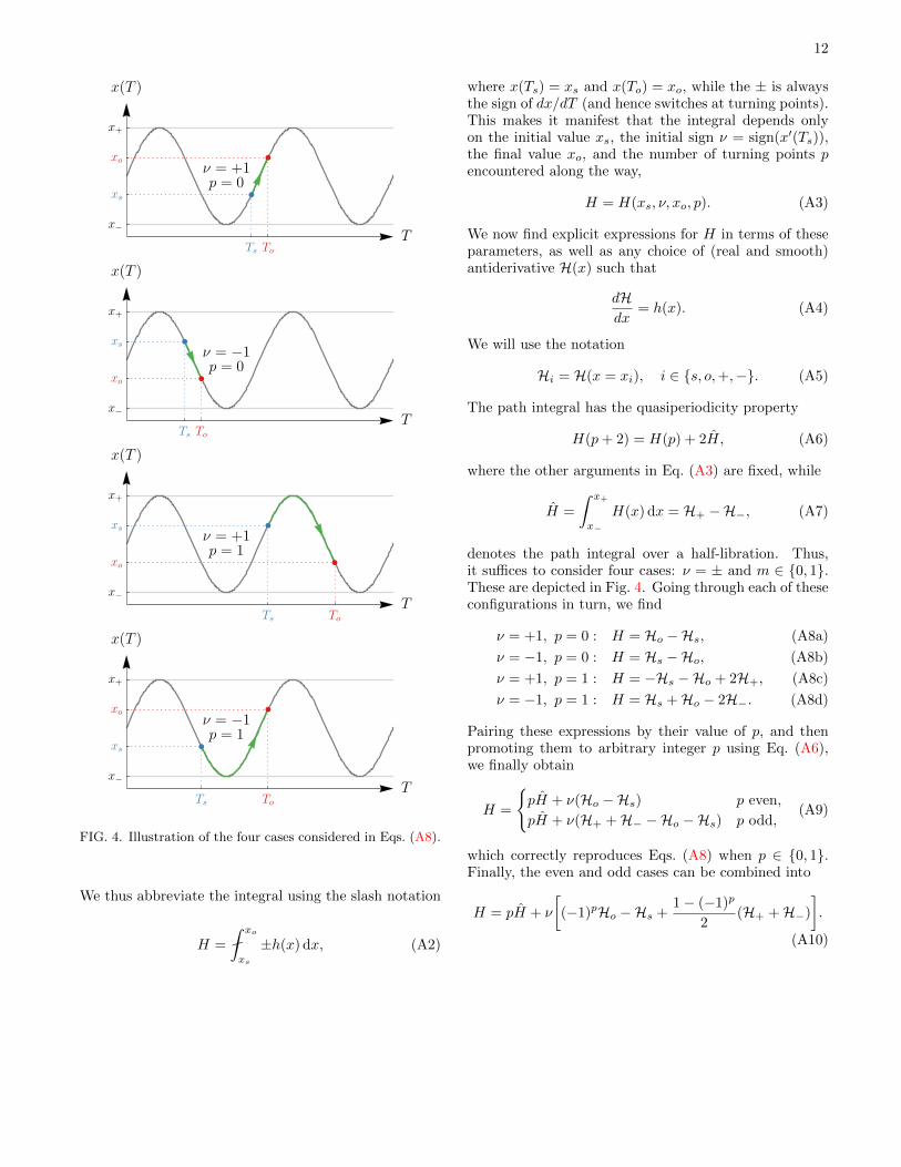
FIG. 4. Illustration of the four cases considered in Eqs. (A8).
We thus abbreviate the integral using the slash notation
H =
xo
xs
±h(x) dx, (A2)
where x(Ts) = xs and x(To) = xo, while the ± is alwaysthe sign of dx/dT (and hence switches at turning points).This makes it manifest that the integral depends onlyon the initial value xs, the initial sign ν = sign(x′(Ts)),the final value xo, and the number of turning points pencountered along the way,
H = H(xs, ν, xo, p). (A3)
We now find explicit expressions for H in terms of theseparameters, as well as any choice of (real and smooth)antiderivative H(x) such that
dHdx
= h(x). (A4)
We will use the notation
Hi = H(x = xi), i ∈ {s, o,+,−}. (A5)
The path integral has the quasiperiodicity property
H(p+ 2) = H(p) + 2H, (A6)
where the other arguments in Eq. (A3) are fixed, while
H =
ˆ x+
x−
H(x) dx = H+ −H−, (A7)
denotes the path integral over a half-libration. Thus,it suffices to consider four cases: ν = ± and m ∈ {0, 1}.These are depicted in Fig. 4. Going through each of theseconfigurations in turn, we find
ν = +1, p = 0 : H = Ho −Hs, (A8a)
ν = −1, p = 0 : H = Hs −Ho, (A8b)
ν = +1, p = 1 : H = −Hs −Ho + 2H+, (A8c)
ν = −1, p = 1 : H = Hs +Ho − 2H−. (A8d)
Pairing these expressions by their value of p, and thenpromoting them to arbitrary integer p using Eq. (A6),we finally obtain
H =
{pH + ν(Ho −Hs) p even,
pH + ν(H+ +H− −Ho −Hs) p odd,(A9)
which correctly reproduces Eqs. (A8) when p ∈ {0, 1}.Finally, the even and odd cases can be combined into
H = pH + ν
[(−1)pHo −Hs +
1− (−1)p
2(H+ +H−)
].
(A10)

13
Appendix B: Radial integrals and inversion
In this appendix, we analyze the radial integrals and trajectories following the approach established in the polarcase in Sec. III. It is convenient to rewrite the radial integrals as
Ir = I0, (B1)
Iφ =2Ma
r+ − r−
[(r+ −
aλ
2M
)I+ −
(r− −
aλ
2M
)I−
], (B2)
It =(2M)2
r+ − r−
[r+
(r+ −
aλ
2M
)I+ − r−
(r− −
aλ
2M
)I−
]+ (2M)2I0 + (2M)I1 + I2, (B3)
where we introduced
I± =
ro
rs
dr
±r(r − r±)√R(r)
, I` =
ro
rs
r` dr
±r√R(r)
, (B4)
for ` ∈ {0, 1, 2}. Note that Ir = I0 and Iσ = I2. The radial trajectory satisfies the squared differential equation
(drodτ
)2
= R(ro(τ)), (B5)
while the radial integrals (B4) satisfy
dI`dτ
= [ro(τ)]`,
dI±dτ
=1
ro(τ)− r±. (B6)
Below we will go through each case (1)-(4) [Sec. IV C], following the basic approach established in our treatmentof the angular integrals in Sec. III above. Each case requires a different substitution of variables to obtain realand smooth antiderivatives for the integrals.9 Many of the relevant substitutions are summarized in §3.145–3.151 ofRef. [19], and full details are presented in §250–267 of Ref. [15]. The antiderivatives can be used to calculate the pathintegrals as functions of rs, ro, νr, and the number of turning points w encountered along the trajectory via
Ii = (−1)wIoi − Isi , (B7)
where Iji indicates the antiderivative Ii evaluated at the source (j = s) or observer (j = o). Here, we assumed thatthe trajectory encounters either no turning points (w = 0) or a single turning point (w = 1), which is appropriate forour restriction to motion in the black hole exterior.
Preliminaries
For the analysis that follows, it is most convenient to think of the radial potential as a quartic in terms of its roots,
R(r) = (r − r1)(r − r2)(r − r3)(r − r4). (B8)
Throughout this section, we use the notation
rij = ri − rj , (B9)
with i, j ∈ {1, 2, 3, 4,+,−} to represent the four roots of the radial potential, as well as the inner and outer horizons.In addition, if r3 = r4 are complex conjugates, then it is useful to set
r3 = b1 − ia1, r4 = b1 + ia1, a1 =
√−r
243
4> 0, b1 =
r3 + r42
= z > 0, (B10)
9Near critical values of the roots, the integrals may be approximated using the method of matched asymptotic expansions [11, 14].
14
where the last equality follows from the explicit expressions (95) for the radial roots, and the following inequalityfrom Eq. (94). Moreover, if r1 = r2 are also complex conjugates, then we likewise set
r1 = b2 − ia2, r2 = b2 + ia2, a2 =
√−r
221
4> 0, b2 =
r1 + r22
= −z < 0. (B11)
Note that the condition r1 + r2 + r3 + r4 = 0 is automatically enforced, as expected from Eq. (96), and also that
b1 > 0 > b2 = −b1, a1 > a2 > 0. (B12)
Lastly, we define once and for all the elliptic parameter
k =r32r41r31r42
. (B13)
Note that if all the roots are real, then their ordering ensures that r32r41 − r31r42 = −r43r21 < 0, and hence that
k ∈ (0, 1). (B14)
On the other hand, if two of the roots are complex, then k ∈ C is a pure complex phase, as can be seen by pluggingin Eqs. (B10) into the definition (B13). When all the roots are complex, then k > 1, as can be seen by plugging inEqs. (B10) and (B11) into the definition (B13). In these cases, another parameter is needed instead.
1. Case (1)
In case (1), all four roots are real and the range of radial motion is r1 < r2 ≤ r ≤ r3 < r4. (In the maximally extendedspacetime, the photon alternates between successive universes.) An appropriate substitution for the evaluation of theintegrals (B4) is then (see Eq. (4) in §3.147 of Ref. [19] and §254 of Ref. [15])
x1(r) =
√r − r2r − r1
r31r32∈ (0, 1]. (B15)
The parameter (B13) is less than unity, k ∈ (0, 1), and the antiderivatives
I0 = F (1)(r), (B16)
I1 = r1F(1)(r) + r21Π
(1)1 (r), (B17)
I2 =
√R(r)
r − r1− r1r4 + r2r3
2F (1)(r)− E(1)(r), (B18)
I± = −Π(1)± (r)− F (1)(r)
r±1, (B19)
are real and smooth, with10
F (1)(r) =2√r31r42
F(
arcsinx1(r)∣∣∣k)≥ 0, (B20)
E(1)(r) =√r31r42E
(arcsinx1(r)
∣∣∣k)≥ 0, (B21)
Π(1)1 (r) =
2√r31r42
Π
(r32r31
; arcsinx1(r)
∣∣∣∣k)≥ 0, (B22)
Π(1)± (r) =
2√r31r42
r21r±1r±2
Π
(r±1r32r±2r31
; arcsinx1(r)
∣∣∣∣k), (B23)
In general, the expression for I2 contains an additional contribution from the antiderivative
r1 + r2 + r3 + r42
(r1F
(1)(r) + r21Π(1)1 (r)
)= 0, (B24)
which in this case vanishes by Eq. (96).
10F (1) ≥ 0, E(1) ≥ 0, and Π(1)1 ≥ 0 because F (ϕ|k) ≥ 0, E(ϕ|k) ≥ 0 and Π(n;ϕ|k) ≥ 0 whenever ϕ ∈
[0, π
2
], k ∈ [0, 1], and n ∈ [0, 1]. On
the other hand, Π(1)± can be negative.
15
a. Inversion for ro(τ)
Before a turning point is reached, the path integral Ir = τ beginning from r = rs is given by
τ = Ir = νr(Ior − Isr ), νr = sign(prs). (B25)
As in the angular analysis of Sec. III, we may use the Jacobi elliptic sine function to invert this equation. Recallingthat Ir = I0 = F (1)(r), Eqs. (37), (B20), and (B25) can be combined to give
x1(ro) = νr sn(X1(τ)
∣∣k), X1(τ) =
√r31r42
2(τ + νrIsr ). (B26)
Solving for ro using Eq. (B15), we then find
r(1)o (τ) =r2r31 − r1r32 sn2
(X1(τ)
∣∣k)
r31 − r32 sn2(X1(τ)
∣∣k) , (B27)
where we write r(1)o to emphasize that this formula for ro(τ) was derived in case (1), even though it will extend to the
other cases with little modification. Although Eq. (B27) was derived under the assumption that a turning point hasnot yet been reached, it in fact continues properly through turning points to provide the full parameterized trajectoryro(τ), as follows. Noting that sn2(ϕ|k) oscillates smoothly between 0 and +1 with period 2K(k), we see that Eq. (B27)defines a trajectory ro(τ) that oscillates between r2 and r3 with period 2K(k). Thus, it has the correct quantitativebehavior at turning points, and we need only check that it satisfies the squared differential equation (B5), which iseasily verified using the elliptic identities (39) and (40). This completes the proof that Eq. (B27) is the unique solutionfor ro(τ) with initial conditions ro(0) = rs and sign[r′o(0)] = νr, which is manifestly real in case (1).
b. Path integrals as a function of Mino time
We have Ir = I0 = τ by definition, and the other path integrals may be expressed in terms of Mino time τ using aslight extension of the method used in Sec. III for the angular case. Before the first turning point is reached, we have
Ii = νr(Ioi − Isi ), (B28)
where the antiderivatives Ii depend on r primarily through the combination arcsinx1(r). Applying the formula (43)to Eq. (B26) extends arcsinx1(r) to the (monotonically increasing in τ) amplitude
arcsinx1(r) = νr am(X1(τ)
∣∣k), (B29)
where X1(τ) is as defined in Eq. (B26), and the restriction |ϕ| ≤ K(k) is satisfied on account of our assumption thata turning point has not yet been reached. Plugging the extension (B29) into Eq. (B28) as needed, we then find
I1 = r1τ + r21Π(1)1,τ , (B30a)
I2 = H(1)τ −
r1r4 + r2r32
τ − E(1)τ , (B30b)
I± = − τ
r±1−Π
(1)±,τ , (B30c)
with
H(1)τ =
r′o(τ)
ro(τ)− r1− νr
√R(rs)
rs − r1, (B31)
E(1)τ =
√r31r42
[E(
am(X1(τ)
∣∣k)∣∣∣k)− νrE
(arcsinx1(rs)
∣∣∣k)], (B32)
Π(1)1,τ =
2√r31r42
[Π
(r32r31
; am(X1(τ)
∣∣k)∣∣∣∣k)− νrΠ
(r32r31
; arcsinx1(rs)
∣∣∣∣k)], (B33)
Π(1)±,τ =
2√r31r42
r21r±1r±2
[Π
(r±1r32r±2r31
; am(X1(τ)
∣∣k)∣∣∣∣k)− νrΠ
(r±1r32r±2r31
; arcsinx1(rs)
∣∣∣∣k)]. (B34)

16
These functions of Mino time vanish at τ = 0 by construction.Although these expressions were derived under the assumption that a turning point does not occur, they in fact
extend properly through turning points to give the complete path integrals Ii, as follows. Since am(ϕ|k), F (ϕ|k),E(ϕ|k), and Π(n;ϕ|k) are real and smooth functions of ϕ provided max(k, n) < 1 (which is the case here), it followsthat the candidate formulas for the Ii are real and smooth. Thus, we need only check the differential equations (B6),which is straightforward using Eq. (B29) together with the quasiperiodicity properties (53). This completes the proofthat these formulas give the full path integrals (B4).
2. Case (2)
In case (2), all four roots are real and the range of radial motion is r1 < r2 < r3 < r4 ≤ r. An appropriatesubstitution for the evaluation of the integrals (B4) is then (see Eq. (8) in §3.147 of Ref. [19] and §258 of Ref. [15])
x2(r) =
√r − r4r − r3
r31r41∈[0,
√r31r41
]⊂ [0, 1). (B35)
The parameter (B13) is less than unity, k ∈ (0, 1), and the antiderivatives
I0 = F (2)(r), (B36)
I1 = r3F(2)(r) + r43Π
(2)1 (r), (B37)
I2 =
√R(r)
r − r3− r1r4 + r2r3
2F (2)(r)− E(2)(r), (B38)
I± = −Π(2)± (r)− F (2)(r)
r±3, (B39)
are real and smooth, with11
F (2)(r) =2√r31r42
F(
arcsinx2(r)∣∣∣k)≥ 0, (B40)
E(2)(r) =√r31r42E
(arcsinx2(r)
∣∣∣k)≥ 0, (B41)
Π(2)1 (r) =
2√r31r42
Π
(r41r31
; arcsinx2(r)
∣∣∣∣k)≥ 0, (B42)
Π(2)± (r) =
2√r31r42
r43r±3r±4
Π
(r±3r41r±4r31
; arcsinx2(r)
∣∣∣∣k), (B43)
In general, the expression for I2 contains an additional contribution from the antiderivative
r1 + r2 + r3 + r42
(r3F
(2)(r) + r43Π(2)1 (r)
)= 0, (B44)
which in this case vanishes by Eq. (96).
a. Inversion for ro(τ)
Before a turning point is reached, the path integral Ir = τ beginning from r = rs is still given by Eq. (B25). Asusual, we may use the Jacobi elliptic sine function to invert this equation. Recalling that Ir = I0 = F (2)(r), Eqs. (37),(B25), and (B40) can be combined to give
x2(ro) = νr sn(X2(τ)
∣∣k), X2(τ) =
√r31r42
2(τ + νrIsr ). (B45)
11F (2) ≥ 0, E(2) ≥ 0, and Π(2)1 ≥ 0 because F (ϕ|k) ≥ 0, E(ϕ|k) ≥ 0 and Π(n;ϕ|k) ≥ 0 whenever ϕ ∈
[0, arcsin 1√
n
], k ∈ [0, 1], and n ≥ 1.
On the other hand, Π(2)± can be negative.

17
Solving for ro using Eq. (B35), we then find
r(2)o (τ) =r4r31 − r3r41 sn2
(X2(τ)
∣∣k)
r31 − r41 sn2(X2(τ)
∣∣k) . (B46)
where we write r(2)o to emphasize that this formula for ro(τ) was derived in case (2), even though it will extend to
the other cases with little modification. Although Eq. (B46) was derived under the assumption that a turning pointhas not yet been reached, it in fact continues properly through the turning point r4 (if encountered) to provide thefull parameterized trajectory ro(τ). (If νr < 0 there is no turning point in the future of the initial data.) Noting thatsn2(ϕ|k) oscillates smoothly between 0 and +1 with period 2K(k), we see that Eq. (B46) defines a trajectory ro(τ)that correctly bounces when r = r4, where sn2(ϕ|k) = 0. Thus, it has the correct quantitative behavior at the turningpoint, and we need only check that it satisfies the squared differential equation (B5), which is easily verified using theelliptic identities (39) and (40). This completes the proof that Eq. (B46) is the unique solution for ro(τ) with initialconditions ro(0) = rs and sign[r′o(0)] = νr, which is manifestly real in case (2).
b. Path integrals as a function of Mino time
We have Ir = I0 = τ by definition, and the other path integrals may be expressed in terms of Mino time τusing the same method as usual. Before the first turning point is reached, we once again have Eq. (B28), wherethe antiderivatives Ii depend on r primarily through the combination arcsinx2(r). Applying the formula (43) toEq. (B45) extends arcsinx2(r) to the (monotonically increasing in τ) amplitude
arcsinx2(r) = νr am(X2(τ)
∣∣k), (B47)
where X2(τ) is as defined in Eq. (B45), and the restriction |ϕ| ≤ K(k) is satisfied on account of our assumption thata turning point has not yet been reached. Plugging the extension (B47) into Eq. (B28) as needed, we then find
I1 = r3τ + r43Π(2)1,τ , (B48)
I2 = H(2)τ −
r1r4 + r2r32
τ − E(2)τ , (B49)
I± = − τ
r±3−Π
(2)±,τ , (B50)
with
H(2)τ =
r′o(τ)
ro(τ)− r3− νr
√R(rs)
rs − r3, (B51)
E(2)τ =
√r31r42
[E(
am(X2(τ)
∣∣k)∣∣∣k)− νrE
(arcsinx2(rs)
∣∣∣k)], (B52)
Π(2)1,τ =
2√r31r42
[Π
(r41r31
; am(X2(τ)
∣∣k)∣∣∣∣k)− νrΠ
(r41r31
; arcsinx2(rs)
∣∣∣∣k)], (B53)
Π(1)±,τ =
2√r31r42
r43r±3r±4
[Π
(r±3r41r±4r31
; am(X2(τ)
∣∣k)∣∣∣∣k)− νrΠ
(r±3r41r±4r31
; arcsinx2(rs)
∣∣∣∣k)]. (B54)
These functions of Mino time vanish at τ = 0 by construction.Although these expressions were derived under the assumption that a turning point does not occur, they in fact
extend properly through the turning point r4 (if encountered) to give the complete path integrals Ii, as follows. Sinceam(ϕ|k), F (ϕ|k), E(ϕ|k), and Π(n;ϕ|k) are real and smooth functions of ϕ provided max(k, n) < 1 (which is the casehere), it follows that the candidate formulas for the Ii are real and smooth. Thus, we need only check the differentialequations (B6), which is straightforward using Eq. (B47) together with the quasiperiodicity properties (53). Thiscompletes the proof that these formulas give the full path integrals (B4).
3. Case (3)
In case (3), only two roots are real and the range of radial motion is r1 < r2 < r− < r+ ≤ ri with r3 = r4. Anappropriate substitution for the evaluation of the integrals (B4) is then (see Eq. (1) in §3.145 of Ref. [19] and §260 of

18
Ref. [15])12
x3(r) =A(r − r1)−B(r − r2)
A(r − r1) +B(r − r2), (B55)
where [recall Eq. (B10)]
A2 = a21 + (b1 − r2)2> 0, B2 = a21 + (b1 − r1)
2> 0, (B56)
and we must choose the same sign for the square root in A and B. Picking the positive branch results in
A =√r32r42 > 0, B =
√r31r41 > 0. (B57)
Moreover, since r3 + r4 = 2z > 0 [Eq. (B10)] and r1 + r2 = −2z < 0 [Eq. (96)], it follows that r3 + r4 > r1 + r2, andhence that B2 −A2 = r21(r3 + r4 − r1 − r2) > 0. Therefore, using the fact that r1 < r2 < r,
B > A > 0, α0 =B +A
B −A > 1, x3(r) =1− B(r−r2)
A(r−r1)
1 + B(r−r2)A(r−r1)
∈(− 1
α0, 1
)⊂ (−1, 1). (B58)
While in this case, the parameter (B13) is a pure phase k ∈ C, we can replace it by a new parameter that is real,positive, and less than unity:
k3 =(A+B)
2 − r2214AB
=1
2
1 +
a21 + (b1 − r1)(b1 − r2)√[a21 + (b1 − r1)(b1 − r2)]
2+ a21r
221
∈ (0, 1). (B59)
We now invoke the results in §341 of Ref. [15] (though note that we use different conventions for the elliptic integrals).After correcting an error in the auxiliary formula §361.54 (their f1 is missing a factor of 1
2 ), we find that whenever
j ∈ (0, 1), α2 > 1, ϕ ∈[0, π − arccos
1
α
), (B60)
so that α2/(α2 − 1
)> j is automatically satisfied, then
R1
(α;ϕ
∣∣j)
=
ˆ F (ϕ|j)
0
du
1 + α cn(u|j) =
ˆ ϕ
0
dt
(1 + α cos t)√
1− j sin2 t(B61)
=1
1− α2
[Π
(α2
α2 − 1;ϕ
∣∣∣∣j)− αf1
], (B62)
R2(α;ϕ|j) =
ˆ F (ϕ|j)
0
du
[1 + α cn(u|j)]2=
ˆ ϕ
0
dt
(1 + α cos t)2√
1− j sin2 t(B63)
=1
α2 − 1
[F(ϕ∣∣j)− α2
j + (1− j)α2
(E(ϕ∣∣j)− α sinϕ
√1− j sin2 ϕ
1 + α cosϕ
)]
+1
j + (1− j)α2
(2j − α2
α2 − 1
)R1
(α;ϕ
∣∣j), (B64)
f1 =p12
log
∣∣∣∣∣p1√
1− j sin2 ϕ+ sinϕ
p1√
1− j sin2 ϕ− sinϕ
∣∣∣∣∣ ≥ 0, p1 =
√α2 − 1
j + (1− j)α2> 0. (B65)
Finally, we also introduce the parameters
α± =Br±2 +Ar±1Br±2 −Ar±1
= − 1
x3(r±). (B66)
12Here, the two references superficially disagree, but they are in fact related by the identity arccosx = 2 arctan
√1−x21+x
, valid for x ∈ (−1, 1].
19
Since the conditions (B60) are satisfied by j = k3, α = α0,±, and ϕ = arccosx3(r), the antiderivatives
I0 = F (3)(r), (B67)
I1 =
(Br2 +Ar1B +A
)F (3)(r) + Π
(3)1 (r), (B68)
I2 =
(Br2 +Ar1B +A
)2
F (3)(r) + 2
(Br2 +Ar1B +A
)Π
(3)1 (r) +
√ABΠ
(3)2 (r), (B69)
I± = − 1
Br±2 +Ar±1
[(B +A)F (3)(r) +
2r21√AB
Br±2 −Ar±1R1
(α±; arccosx3(r)
∣∣∣k3)], (B70)
are real and smooth, with13
F (3)(r) =1√AB
F(
arccosx3(r)∣∣∣k3)> 0, (B71)
Π(3)` (r) =
(2r21√AB
B2 −A2
)`R`
(α0; arccosx3(r)
∣∣∣k3)> 0. (B72)
a. Inversion for ro(τ)
Before a turning point is reached, the path integral Ir = τ beginning from r = rs is still given by Eq. (B25), whichin this case can be inverted using the Jacobi elliptic cosine function cn(ϕ|k). This function satisfies
cn(F (arccosϕ|k)) = ϕ, (B73)
and is even in its first argument, cn(−ϕ|k) = cn(ϕ|k). Recalling that Ir = I0 = F (3)(r), Eqs. (B25), (B71), and (B73)can be combined to give
x3(ro) = cn(X3(τ)
∣∣k3), X3(τ) =
√AB(τ + νrIsr ). (B74)
Solving for ro using Eq. (B55), we then find
r(3)o (τ) =(Br2 −Ar1) + (Br2 +Ar1) cn
(X3(τ)
∣∣k3)
(B −A) + (B +A) cn(X3(τ)
∣∣k3) , (B75)
where we write r(3)o to emphasize that this formula for ro(τ) was derived in case (3), even though it will extend to the
other cases with little modification. This trajectory never encounters a turning point outside the horizon, and henceEq. (B75) is the unique solution for ro(τ) with initial conditions ro(0) = rs and sign[r′o(0)] = νr, which is manifestlyreal in case (3).
b. Path integrals as a function of Mino time
We have Ir = I0 = τ by definition, and the other path integrals may be expressed in terms of Mino time τ usingthe same method as usual. Since there are no turning points, we once again have Eq. (B28), where the antiderivativesIi depend on r primarily through the combination arccosx3(r). We now invoke the inversion formula
am(ϕ|k) = arccos(cn(ϕ|k)), 0 ≤ ϕ ≤ 2K(k). (B76)
Applying it to Eq. (B74) extends arccosx3(r) to the (monotonically increasing in τ) amplitude
arccosx3(r) = am(X3(τ)
∣∣k), (B77)
13F (3) > 0 and Π(3)k > 0 because F (ϕ|j) ≥ 0 and Rk(α;ϕ|j) ≥ 0 whenever ϕ ∈
[0, π − arccos 1
α
], j ∈ (0, 1), and α > 1 (in the case of Rk,
this is manifest from the integrand). Note however that if α < −1, then R1 ≤ 0 changes sign while R2 ≥ 0 does not.
20
where X3(τ) is as defined in Eq. (B74), and the restriction 0 ≤ ϕ ≤ 2K(k) is satisfied on the whole range of motion.Plugging the extension (B77) into Eq. (B28) as needed, we then find
I1 =
(Br2 +Ar1B +A
)τ + Π
(3)1,τ , (B78)
I2 =
(Br2 +Ar1B +A
)2
τ + 2
(Br2 +Ar1B +A
)Π
(3)1,τ +
√ABΠ
(3)2,τ , (B79)
I± = − (B +A)τ + Π(3)±,τ
Br±2 +Ar±1, (B80)
with
Π(3)`,τ =
(2r21√AB
B2 −A2
)`[R`
(α0; am
(X3(τ)
∣∣k3)∣∣∣k3
)− νrR`
(α0; arccosx3(rs)
∣∣∣k3)], (B81)
Π(3)±,τ =
(2r21√AB
Br±2 −Ar±1
)[R1
(α±; am
(X3(τ)
∣∣k3)∣∣∣k3
)− νrR1
(α±; arccosx3(rs)
∣∣∣k3)]. (B82)
These functions of Mino time vanish at τ = 0 by construction. Since a turning point never occurs, these formulasgive the full path integrals (B4).
4. Case (4)
In case (4), there are two pairs r1 = r2 and r3 = r4 of complex conjugate roots and the range of radial motionis unbounded. An appropriate substitution for the evaluation of the integrals (B4) is then (see Eq. (4) in §3.145 ofRef. [19] and §267 of Ref. [15])14
x4(r) =r − b2a2
=r + b1a2
> 0, (B83)
where we used the fact that b2 = −b1 = −z < 0 [Eq. (B11)], so that r > 0 > −b1 outside the horizon; since a2 > 0[Eq. (B12)], this guarantees that x4(r) is positive. In principle, we could have equivalently defined x4(r) = (r − b1)/a1,but then we would also have had to consider negative values of x4(r). The present choice will prove more convenient.
Following Refs. [15, 19], we must also introduce the quantities [recall Eqs. (B10) and (B11)]
C2 = (a1 − a2)2
+ (b1 − b2)2> 0, D2 = (a1 + a2)
2+ (b1 − b2)
2> 0, (B84)
which are well-defined up to a choice of sign in the square root. Picking the positive branch results in
C =√r31r42 > 0, D =
√r32r41 > 0, (B85)
from which it then follows that
k =D2
C2= 1 +
4a1a2
(a1 − a2)2
+ (b1 − b2)2 > 1. (B86)
While the parameter k > 1, we can replace it by a new elliptic parameter that is real, positive, and less than unity:
k4 =4CD
(C +D)2 =
4√k
(1 +√k)2 ∈ (0, 1). (B87)
14Here, the two references superficially disagree, but they are in fact related by the arctangent addition formula. However, the use of thisformula in Ref. [15] introduces a discontinuity in the antiderivative, so we instead use its always continuous form given in Ref. [19].
21
The reduction of the elliptic integrals (B4) to Legendre normal form presented in Refs. [15, 19] further requires15
g0 =
√4a22 − (C −D)
2
(C +D)2 − 4a22
∈ (0, 1), (B88)
with the last inequality rendered manifest by the relations [recall from Eq. (B12) that a1 > a2 > 0]
g20 =1− Z1 + Z
, Z =a21 − a22 + (b1 − b2)
2
CD∈ (0, 1),
√1− Z2 =
2a1(b1 − b2)
CD∈ (0, 1). (B89)
We now invoke the results in §342 of Ref. [15] (though note that we use different conventions for the elliptic integrals).After correcting a typo in the auxiliary formula §361.64 (the second square root in the denominator of f2 should only
include√
1 + α2), we find that whenever
j ∈ (0, 1), α ∈ R, ϕ ∈(−π
2+ arctanα,
π
2+ arctanα
), (B90)
so that(1 + α2
)(1− j + α2
)> 0 is automatically satisfied, then
S1
(α;ϕ
∣∣j)
=
ˆ F (ϕ|j)
0
du
1 + α sc(u|j) =
ˆ ϕ
0
dt
(1 + α tan t)√
1− j sin2 t(B91)
=1
1 + α2
[F(ϕ∣∣j)
+ α2Π(
1 + α2;ϕ∣∣j)− αf2
], (B92)
S2(α;ϕ|j) =
ˆ F (ϕ|j)
0
du
[1 + α sc(u|j)]2=
ˆ ϕ
0
dt
(1 + α tan t)2√
1− j sin2 t(B93)
= − 1
(1 + α2)(1− j + α2)
[(1− j)F
(ϕ∣∣j)
+ α2E(ϕ∣∣j)
+α2√
1− j sin2 ϕ(α− tanϕ)
1 + α tanϕ− α3
]
+
(1
1 + α2+
1− j1− j + α2
)S1
(α;ϕ
∣∣j), (B94)
f2 =p22
log
∣∣∣∣∣1− p21 + p2
1 + p2√
1− j sin2 ϕ
1− p2√
1− j sin2 ϕ
∣∣∣∣∣ ≥ 0, p2 =
√1 + α2
1− j + α2> 0. (B95)
Finally, we also introduce the parameters
g± =g0x4(r±)− 1
g0 + x4(r±). (B96)
Since the conditions (B90) are satisfied by j = k4, α = g0,±, and ϕ = arctanx4(r) + arctan g0, the antiderivatives
I0 = F (4)(r), (B97)
I1 =
(a2g0− b1
)F (4)(r)−Π
(4)1 (r), (B98)
I2 =
(a2g0− b1
)2
F (4)(r)− 2
(a2g0− b1
)Π
(4)1 (r) + Π
(4)2 (r), (B99)
I± =g0
a2[1− g0x4(r±)]
[F (4)(r)− 2
C +D
(1 + g20
g0[g0 + x4(r±)]
)S1
(g±; arctanx4(r) + arctan g0
∣∣∣k4)], (B100)
are real and smooth, with16
F (4)(r) =2
C +DF(
arctanx4(r) + arctan g0
∣∣∣k4)> 0, (B101)
Π(4)` (r) =
2
C +D
[a2g0
(1 + g20
)]`S`
(g0; arctanx4(r) + arctan g0
∣∣∣k4). (B102)
15This definition agrees with Ref. [19] (g0 = tanα) and Ref. [15] (g20 = g21), except that a2 replaces a1 because our x4(r) is (r − b2)/a2
instead of (r − b1)/a1. Unfortunately, g0 = ±√g20 exhibits a sign ambiguity in the choice of branch for the square root. This has led some
authors such as Dexter & Agol [7] to prefer the use of Carlson’s symmetric integrals, which notably do not suffer from this sign ambiguity[20]. However, in the present case, picking the positive branch in the formulas of Ref. [15] always yields the correct answer.
16F (4) > 0 and Π(4)2 > 0 because F (ϕ|j) ≥ 0 and S2(α;ϕ|j) ≥ 0 whenever ϕ ∈
[0, π
2+ arctanα
], j ∈ (0, 1), and α > 0 (in the case of S2, this
is manifest from the integrand). On the other hand, S1 (and therefore Π(4)1 > 0) can in principle be negative as r →∞ and x4(r)→ π
2.

22
a. Inversion for ro(τ)
Before a turning point is reached, the path integral Ir = τ beginning from r = rs is still given by Eq. (B25), which inthis case can be inverted using the Jacobi elliptic tangent function sc(ϕ|k) = sn(ϕ|k)/ cn(ϕ|k). This function satisfies
sc(F (arctanϕ|k)) = ϕ, (B103)
and is odd in its first argument, sc(−ϕ|k) = sc(ϕ|k). Recalling that Ir = I0 = F (4)(r), Eqs. (B25) and (B101) can becombined to give
F(
arctanx4(ro) + arctan g0
∣∣∣k4)
= X4(τ), X4(τ) =C +D
2(νrτ + Isr ). (B104)
At this stage, we need to invoke the arctangent addition formula
arctanx+ arctan y = arctan
(x+ y
1− xy
)+ nπ, n ∈ Z, (B105)
(with the precise value of the integer n depending on the range of x, y ∈ R), to reexpress the last equation as
X4(τ) = F
(arctan
(g0 + x4(ro)
1− g0x4(ro)
)+ nπ
∣∣∣∣k4)
= F
(arctan
(g0 + x4(ro)
1− g0x4(ro)
)∣∣∣∣k4)
+ 2nK(k4), (B106)
where the last step follows from the quasiperiodicity property F (ϕ+nπ|k) = F (ϕ|k) + 2nK(k) of the elliptic integralof the first kind [see Eqs. (53)]. Thus, we have established that
F
(arctan
(g0 + x4(ro)
1− g0x4(ro)
)∣∣∣∣k4)
= X4(τ)− 2nK(k4), (B107)
for some integer n ∈ Z. Applying the formula (B103), it then results that
g0 + x4(ro)
1− g0x4(ro)= sc
(X4(τ)− 2nK(k4)
∣∣∣k4)
= sc(X4(τ)
∣∣k4), (B108)
where in the last step, we used the periodicity property sc(ϕ + 2K(k)|k) = sc(ϕ|k). Solving for ro using Eq. (B83),we then find
r(4)o (τ) = −a2[g0 − sc
(X4(τ)
∣∣k4)
1 + g0 sc(X4(τ)
∣∣k4)]− b1, (B109)
where we write r(4)o to emphasize that this formula for ro(τ) was derived in case (4), even though it will extend to the
other cases with little modification. This trajectory never encounters a turning point outside the horizon, and henceEq. (B109) is the unique solution for ro(τ) with initial conditions ro(0) = rs and sign[r′o(0)] = νr, which is manifestlyreal in case (4).
b. Path integrals as a function of Mino time
We have Ir = I0 = τ by definition, and the other path integrals may be expressed in terms of Mino time τ usingthe same method as usual. Since there are no turning points, we once again have Eq. (B28), where the antiderivativesIi depend on r primarily through the combination arctanx4(r) + arctan g0. We now invoke the inversion formula
am(F (ϕ|k)|k) = ϕ. (B110)
Applying it to Eq. (B104) extends arctanx4(r) + arctan g0 to the (monotonically increasing in τ) amplitude
arctanx4(r) + arctan g0 = am(X4(τ)
∣∣k), (B111)

23
where X4(τ) is as defined in Eq. (B104). Plugging the extension (B111) into Eq. (B28) as needed, we then find
I1 =
(a2g0− b1
)τ −Π
(4)1,τ , (B112)
I2 =
(a2g0− b1
)2
τ − 2
(a2g0− b1
)Π
(4)1,τ + Π
(4)2,τ , (B113)
I± =g0
a2[1− g0x4(r±)]
(τ −Π
(4)±,τ
), (B114)
with
Π(4)`,τ =
2νrC +D
[a2g0
(1 + g20
)]`[S`
(g0; am
(X4(τ)
∣∣k4)∣∣∣k4
)− S`
(g0; arctanx4(rs) + arctan g0
∣∣∣k4)], (B115)
Π(4)±,τ =
2νrC +D
(1 + g20
g0[g0 + x4(r±)]
)[S1
(g±; am
(X4(τ)
∣∣k4)∣∣∣k4
)− S1
(g±; arctanx4(rs) + arctan g0
∣∣∣k4)]. (B116)
These functions of Mino time vanish at τ = 0 by construction. Since a turning point never occurs, these formulasgive the full path integrals (B4).
5. Unified inversion formula
Although the inversion formulas r(i)o (τ) derived in the four cases (1)-(4) appear superficially different, their expres-
sions (B27), (B46), (B75), and (B109) are in fact mathematically equivalent after certain sign flips in νr. Thus, eitherone may be used across all four cases (with appropriate sign flips), even though it is only manifestly real in its owndomain of definition.
To prove this, it suffices to show that for each i ∈ {1, 2, 3, 4}, the function ro(τ) = r(i)o (τ) always satisfies the squared
differential equation (B5) with the correct initial position. One can then check the initial sign of the derivative andsend νr → −νr if necessary. For instance, for the inversion formula (B46) derived in case (2), one has
dr(2)o
dτ=r31r41r43
√r31r42 sn
(X2(τ)
∣∣k)
cn(X2(τ)
∣∣k)
dn(X2(τ)
∣∣k)
[r31 − r41 sn
(X2(τ)
∣∣k)]2 , (B117)
R(r(2)o (τ)
)=r331r
241r
243r42 sn2
(X2(τ)
∣∣k)[
1− sn2(X2(τ)
∣∣k)][
1− k sn2(X2(τ)
∣∣k)]
[r31 − r41 sn
(X2(τ)
∣∣k)]4 . (B118)
These expressions manifestly satisfy Eq. (B5), in light of the elliptic identities (39) and (40). Hence, r(2)o (τ) remains
valid in all cases, up to a possible sign flip in νr.17 We can fix the sign ambiguity in νr by careful examination of
Eq. (B117). By construction, the initial sign of the radial momentum in case (2) is sign(prs) = νr. An explicit buttedious computation reveals this to still hold in cases (3) and (4); on the other hand, a sign flip is required for case(1), in which sign(prs) = −νr. Thus a unified inversion formula holding in all cases is
r(2)o (τ) =r4r31 − r3r41 sn2
(X2(τ)
∣∣k)
r31 − r41 sn2(X2(τ)
∣∣k) , X2(τ) =
√r31r42
2(τ + ανrIsr ). (B119)
where α = −1 in case (1) and α = +1 in all other cases (2)-(4). Here, Isr refers to the case (2) antiderivative (B36).
[1] B. Carter, “Global Structure of the Kerr Family of Gravitational Fields,” Physical Review 174 no. 5, (Oct, 1968)1559–1571.
17An almost identical derivation goes through for r(1)o (τ) and r
(3)o (τ), so we omit it here. We did not analytically complete the proof for
r(4)o (τ), which seems to require complicated elliptic identities, but we have numerically checked that it also remains valid in all cases. On
the other hand, it is easy to explicitly check that r(i)o (0) = rs always holds for all i ∈ {1, 2, 3, 4}.

24
[2] J. M. Bardeen, “Timelike and null geodesics in the Kerr metric.,” in Black Holes (Les Astres Occlus), C. Dewitt andB. S. Dewitt, eds., pp. 215–239. Gordon and Breach Science Publishers, Jan, 1973.
[3] B. O’Neill, The geometry of Kerr black holes. A K Peters, Ltd., 1995.[4] S. Chandrasekhar, The mathematical theory of black holes. Oxford University Press, 1983.[5] E. Hackmann, Geodesic equations in black hole space-times with cosmological constant. PhD thesis, Bremen University,
2010. http://elib.suub.uni-bremen.de/diss/docs/00011880.pdf.[6] K. P. Rauch and R. D. Blandford, “Optical Caustics in a Kerr Spacetime and the Origin of Rapid X-Ray Variability in
Active Galactic Nuclei,” ApJ 421 (Jan, 1994) 46.[7] J. Dexter and E. Agol, “A Fast New Public Code for Computing Photon Orbits in a Kerr Spacetime,” ApJ 696 no. 2,
(May, 2009) 1616–1629, arXiv:0903.0620 [astro-ph.HE].[8] D. Kapec and A. Lupsasca, “Particle motion near high-spin black holes,” arXiv e-prints (May, 2019) arXiv:1905.11406,
arXiv:1905.11406 [hep-th].[9] Event Horizon Telescope Collaboration, K. Akiyama, A. Alberdi, W. Alef, K. Asada, R. Azulay, A.-K. Baczko, D. Ball,
M. Balokovic, and J. Barrett, “First M87 Event Horizon Telescope Results. I. The Shadow of the Supermassive BlackHole,” ApJ 875 no. 1, (Apr, 2019) L1, arXiv:1906.11238 [astro-ph.GA].
[10] Y. Mino, “Perturbative approach to an orbital evolution around a supermassive black hole,” Phys. Rev. D 67 no. 8,(Apr, 2003) 084027, arXiv:gr-qc/0302075 [gr-qc].
[11] S. E. Gralla and A. Lupsasca, “Lensing by Kerr Black Holes.” To appear concurrently.[12] M. Abramowitz and I. A. Stegun, Handbook of Mathematical Functions. United States Department of Commerce,
National Institute of Standards and Technology, 1972.[13] D. Gates, D. Kapec, A. Lupsasca, Y. Shi, and A. Strominger, “Polarization Whorls from M87 at the Event Horizon
Telescope,” arXiv e-prints (Sep, 2018) arXiv:1809.09092, arXiv:1809.09092 [hep-th].[14] S. E. Gralla, A. Lupsasca, and A. Strominger, “Observational signature of high spin at the Event Horizon Telescope,”
MNRAS 475 no. 3, (Apr, 2018) 3829–3853, arXiv:1710.11112 [astro-ph.HE].[15] P. F. Byrd and M. Friedman, “Handbook of Elliptic Integrals for Engineers and Physicists (Ref. U. Wegner),”
Mitteilungen der Astronomischen Gesellschaft Hamburg 5 (Jan, 1954) 99.[16] S. E. Vazquez and E. P. Esteban, “Strong-field gravitational lensing by a Kerr black hole,” Nuovo Cimento B Serie 119
no. 5, (May, 2004) 489, arXiv:gr-qc/0308023 [gr-qc].[17] S. Drasco and S. A. Hughes, “Rotating black hole orbit functionals in the frequency domain,” Phys. Rev. D 69 no. 4,
(Feb, 2004) 044015, arXiv:astro-ph/0308479 [astro-ph].[18] R. Fujita and W. Hikida, “Analytical solutions of bound timelike geodesic orbits in Kerr spacetime,” Classical and
Quantum Gravity 26 no. 13, (Jul, 2009) 135002, arXiv:0906.1420 [gr-qc].[19] I. S. Gradshteyn, I. M. Ryzhik, A. Jeffrey, and D. Zwillinger, Table of Integrals, Series, and Products. Academic Press,
2007.[20] B. C. Carlson, “A table of elliptic integrals,” Mathematics of Computation 59 no. 199, (Jul, 1992) 165–180.