Leftist heap: is a binary tree with the normal heap ordering property, but the tree is

not balanced. In fact it attempts to be very unbalanced!

Definition: the null path length npl(x) of node x is the length of the shortest path

from x to a node without two children.

The null path lengh of any node is 1 more than the minimum of the null path lengths

of its children. (let npl(nil)=-1).

Only the tree on the left is leftist.

Null path lengths are shown in the nodes.

Definition: the leftist heap property is that for every node x in the heap, the null

path length of the left child is at least as large as that of the right child.

This property biases the tree to get deep towards the left. It may generate very

unbalanced trees, which facilitates merging!

It also also means that the right path down a leftist heap is as short as any path in the

heap. In fact, the right path in a leftist tree of N nodes contains at most lg(N+1)

nodes. We perform all the work on this right path, which is guaranteed to be short.

Merging on a leftist heap. (Notice that an insert can be considered as a merge of a

one-node heap with a larger heap.)

1. (Magically and recursively) merge the heap with the larger root (6) with the right

subheap (rooted at 8) of the heap with the smaller root, creating a leftist heap.

Make this new heap the right child of the root (3) of h1.

The resulting heap is not leftest at the root. (The npl of 3's left subtree is less than

the npl of 3's right subtree.) Simply swap the root's left and right children.

Working only on the right paths, the time to merge is the sum of the length of the

right paths. Thus, we obtain a O(lgn) bound.

The time for deleteMin is also O(lgN): destroy the root and merge the two heaps.

The time for building a leftist heap is also O(N).

Skew heap: is another self-adjusting data structure, like the splay tree.

Skew heaps are binary trees with heap order, but no structural constraint. Unlike

leftist heaps, no information is maintained about npl and the right path of a skew

heap can be arbitrarily long at any time.

This implies that the worst case running time of all operations is O(N).

However, m consecutive operations take a total worst case time of O(mlgn), an

amortized cost of O(lgn) per operation.

Merging on skew heaps. Merging is performed exactly as it was with leftist heaps,

with one exception.

For skew heaps we always swap the left and right children, regardless of whether

they satisfy the leftist heap order property (the right paths become the new left path)

with the exception that the largest of all the nodes on the right path does not have its

children swapped.

Skew Heaps H1 and H2:

Merge H2 with H1’s right subheap:

Make this heap the left child of H1 and the old left child of H1 becomes the new

right child:

The result is a leftist tree.

But if we insert 15 into this heap, the result would not be leftist.

Comparing leftist and skew heaps with binary heaps:

- leftist and skew heaps: merge, insert, and deleteMin in effectively O(lgn) time

- binary heaps support insert in constant average time per operation.

Binomial queues: support merge, insert, and deleteMin in worst case O(lgn) time

per operation and insert in constant average time per operation.

A binomial queue is a collection of heap-ordered binomial trees, known as a forest.

Facts about binomial trees:

A binomial tree bk of height k is formed by attaching a binomial tree bk-1 to the root

of another binomial tree, bk-1.

There is at most one binomial tree of every height.

Binomial trees of height k have exactly 2k nodes.

The number of nodes at depth d is the binomial coefficient () = "k choose d" =

k!/(d!(k-d)!)

A priority queue of any size can be represented by a collection of binomial trees.

Example 1: 1310 = 11012 ==> 13 can be represented by the forest b3, b2, b0.

Example 2: 610 = 110 ==> the forest b2, b1.

Binomial queue operations:

findMin:

- sequential search of the roots of all the trees ==> O(lgn) time.

- if we maintain information about the minimum root ==> O(1) time.

Merge: O(lgn) worst case. (Merging two trees takes constant time and there are

O(lgn) binomial trees.)

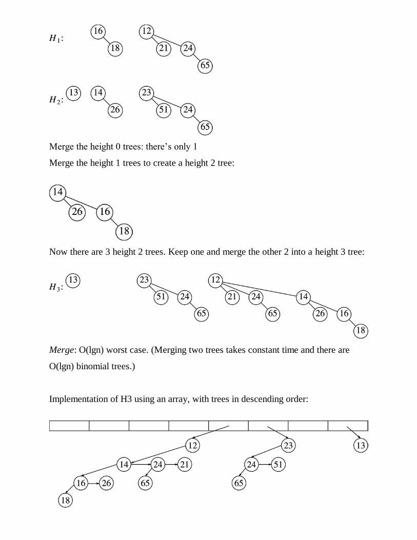
Merge the height 0 trees: there’s only 1

Merge the height 1 trees to create a height 2 tree:

Now there are 3 height 2 trees. Keep one and merge the other 2 into a height 3 tree:

Merge: O(lgn) worst case. (Merging two trees takes constant time and there are

O(lgn) binomial trees.)

Implementation of H3 using an array, with trees in descending order:

insert: a special case of merging a one-node tree.

- O(lgN) worst case. O(1) average case. (Stop when you find a missing Bi tree.)

- Perform N inserts on an initially empty tree in O(N) time.

deleteMin: O(lgN) worst case.

Let H =

Find tree Bk with smallest root (12). Remove Bk from H to form H’.

Remove root from Bk to get H”

Merge H’ and H”:

Series of O(lgN) operations O(lgN).

Splay Trees

Splay trees: instead of maintaining a balanced tree, after a node is accessed, it is

pushed closer to the root, and so are other nodes on the path from the root.

Splaying results in a "flatter" tree - the accessed node is moved to the root, and the

depths of most nodes on the access path are roughly halved. (If a node takes a long

time to access, it will be moved so that it will be accessed quicker next time.)

The splay operations are similar to the AVL rotate operations, but no balancing

information need be maintained.

A single operation in a splay tree may take O(n) time.

However, m consecutive operations are guaranteed to take at most O(mlgn) time.

We say that a splay tree has O(lgn) amortized cost per operation. Over a long

sequence of operations, some may take more, some less.

Example: K5

/ \

K4 F

/ \

K3 E

/ \

K2 D

/ \

A K1

/ \

B C

Access K1: Perform AVL double rotation with K1, K2 (K1’s parent), and K3 (K1’s

grandparent). Move K1 up:

K5 K1

/ \ / \

K4 F K2 K4

/ \ / \ / \

K1 E A B K3 K5

/ \ / \ / \

K2 K3 C D E F

/ \ / \

A B C D

Keep moving K1 up until K1 becomes root. Depth of nodes along access path (from

original root to K1) has roughly been halved. Some shallow nodes were pushed

down two levels, e.g. K5.

Skip Lists Operation Time Complexity

Insertion O(log N)

Removal O(log N)

Contains O(log N)

Enumerate in order

Also:

O(N)

Find the element in the set that is closest to some given value, in O(log N) time.

Find the k-th largest element in the set, in O(log N) time. Requires a simple augmentation

of the the skip list with partial counts.

Count the number of elements in the set whose values fall into a given range, in O(log N)

time. Also requires a simple augmentation of the skip list.

Sorted singly-linked list (O(N)):

Enumerate in order O(N)

Why so slow? It takes so long to get into its middle, so:

=> add a level-2 list that skips every other node.

add a level-3 list that skips every other node in the level-2 list.

…etc

Looks like a binary tree!

Searching is now like a O(lgN) binary search:

first look in the top-most list - move to the right but don’t jump too far.

If can’t move further right on a particular level, drop to the next lower level, which has

shorter jumps.

Search for 8:

Since we landed on a 7, but we were looking for an 8, that means that 8 is not in the set.

How to implement insertions and removals efficiently?

A probabilistic approach: Instead of ensuring that the level-2 list skips every other node, a skip list

is designed in a way that the level-2 list skips one node on average. In some places, it may skip

two nodes, and in other places, it may not skip any nodes

Here is an example of what a skip list may look like:

Insertion: decide how many lists will this node be a part of. With a probability of 1/2,

make the node a part of the lowest-level list only. With 1/4 probability, the node will be a

part of the lowest two lists. With 1/8 probability, the node will be a part of three lists. And

so forth. Insert the node at the appropriate position in the lists that it is a part of.

Deletion: remove the node from all sorted lists that it is a part of.

Contains: we can use the O(log N) algorithm similar described above on multi-level lists.

And, all of these operations are pretty simple to implement in O(log N) time!