nullification of knots and links · june 3, 2011 2:58 wspc/instruction file...

June 3, 2011 2:58 WSPC/INSTRUCTION FILE JKTRnullification6˙2˙11

Journal of Knot Theory and Its Ramificationsc© World Scientific Publishing Company

NULLIFICATION OF KNOTS AND LINKS

YUANAN DIAO

Department of MathematicsUniversity of North Carolina at Charlotte

Charlotte, NC 28223, [email protected]

CLAUS ERNST and ANTHONY MONTEMAYOR

Department of Mathematics and Computer ScienceWestern Kentucky University

Bowling Green, KY 42101, [email protected]

[email protected]

ABSTRACT

It is known that a knot/link can be nullified, i.e., can be made into the trivialknot/link, by smoothing some crossings in a projection diagram of the knot/link. Thenullification of knots/links is believed to be biologically relevant. For example, in DNAtopology, the nullification process may be the pathway for a knotted circular DNA tounknot itself (through recombination of its DNA strands). The minimum number ofsuch crossings to be smoothed in order to nullify the knot/link is called the nullificationnumber. It turns out that there are several different ways to define such a number, sincedifferent conditions may be applied in the nullification process. We show that thesedefinitions are not equivalent, thus they lead to different nullification numbers for aknot/link in general, not just one single nullification number. Our aim is to explore themathematical properties of these nullification numbers. First, we give specific examplesto show that the nullification numbers we defined are different. We provide detailedanalysis of the nullification numbers for the well known 2-bridge knots and links. Wealso explore the relationships among the three nullification numbers, as well as theirrelationships with other knot invariants. Finally, we study a special class of links, namelythose links whose general nullification number equals one. We show that such links existin abundance. In fact, the number of such links with crossing number less than or equalto n grows exponentially with respect to n.

Keywords: knots, links, crossing number, unknotting number, nullification, nullificationnumber.

Mathematics Subject Classification 2000: 57M25

1. Introduction and basic concepts

Although knot theory is a branch of pure mathematics, many questions and studiesthere are motivated by questions from sciences. In fact, the original study of knotsby Lord Kelvin and Tait was motivated by problems from physics. The discovery

1


2 Y. Diao, C. Ernst and A. Montemayor

of DNA knots in recent decades is a late example of a source of many interestingnew questions and research topics in knot theory. It turned out that the topologyof the circular DNA plays a very important role in the properties of the DNA.Various geometric and topological complexity measures of DNA knots that arebelieved to be biologically relevant, such as the knot types, the 3D writhe, theaverage crossing numbers, the average radius of gyration, have been studied. Inthis paper, we are interested in another geometric/topological measure of knotsand links called the nullification number, which is also believed to be biologicallyrelevant [2,11]. Intuitively, this number measures how easily a knotted circular DNAcan unknot itself through recombination of its DNA strands. It turns out that thereare several different ways to define such a number. These different definitions leadto different versions of a nullification number that are related. Our aim is to explorethe mathematical properties of the different versions of the nullification number. Inthis section, we will outline a brief introduction to basic knot theory concepts. InSection 2, we will give precise definitions for three different versions of a nullificationnumber. In Section 3, we will study the nullification number for a well known classof knots called the class of Montesinos knots and links. In Section 4, we explore therelationships among the three versions of a nullification number, as well as theirrelationships with other knot invariants. In particular, we give examples to showthat the three versions of a nullification number defined here are indeed different.In Section 5, we study a special class of links, namely the links whose generalnullification number equals one. There we show that such links exist in abundance.In fact, the number of such links with crossing number less than or equal to n growsexponentially with respect to n.

Let K be a tame link, that is, K is a collection of several piece-wise smoothsimple closed curves in R3. In the particular case that K contains only one com-ponent, it is called a knot instead. However through out this paper a link alwaysincludes the special case that it may be a knot, unless otherwise stated. A link isoriented if each component of the link has an orientation. Intuitively, if one cancontinuously deform a tame link K1 to another tame link K2 (in R3), then K1

and K2 are considered equivalent links in the topological sense. The correspond-ing continuous deformation is called an ambient isotopy, and K1, K2 are said tobe ambient isotopic to each other. The set of all (tame) links that are ambientisotopic to each other is called a link type. For a fixed link (type) K, a link dia-gram of K is a projection of a member K ∈ K onto a plane. Such a projectionp : K ⊂ R3 → D ⊂ R2 is regular if the set of points {x ∈ D : |p−1(x)| > 1} isfinite and there is no x in D for which |p−1(x)| > 2. In other words, in the diagramno more than two arcs of D cross at any point in the projection and there are onlyfinitely many points where the arcs cross each other. A point where two arcs of D

cross each other is called a crossing point, or just a crossing of D. The number ofcrossings in D not only depends on the link type K, it also depends on the geomet-rical shape of the member K representing K and the projection direction chosen.


Nullification of knots and links 3

The minimum number of crossings in all regular projections of all members of Kis called the crossing number of the link type K and is denoted by Cr(K). For anymember K of K, we also write Cr(K) = Cr(K). Of course, by this definition, ifK1 and K2 are of the same link type, then we have Cr(K1) = Cr(K2). However,it may be the case that for a member K of K, none of the regular projections ofK has crossing number Cr(K). A diagram D of a link K ∈ K is minimum if thenumber of crossings in the diagram equals Cr(K). We will often call D a minimumprojection diagram. A link diagram is alternating if one encounters over-passes andunder-passes alternatingly when traveling along the link projection. A diagram D

is said to be reducible if there exists a crossing point in D such that removing thiscrossing point makes the remaining diagram two disconnected parts. D is reducedif it is not reducible. A link is alternating if it has a reduced alternating diagram. Afamous result derived from the Jones polynomial is that the crossing number of analternating link K equals the number of crossings in any of its reduced alternatingdiagram since each diagram is minimum. For example the diagram of the knot K1

in Figure 1 is minimum.

A link K is called a composite link if a member of it can be obtained by cuttingopen two nontrivial links K1 and K2 and reconnecting the strings as shown inFigure 1. The resulting link is written as K = K1#K2 and K1, K2 are called theconnected sum components of K. Of course a link can have more than two connectedsum components. A link K that is not a composite link is called a prime link.

K

+

K1 K2

Fig. 1. A composite knot K = K1#K2.

In the case of alternating links, any two minimum projection diagrams D andD′ of the same alternating link K are flype equivalent, that is, D can be changedto D′ through a finite sequence of flypes [19,20] (see Figure 2).

Let c be a crossing in an alternating diagram D. The flyping circuit of c isdefined as the unique decomposition of D into crossings c1, c2, . . . , cm, m ≥ 1 andtangle diagrams T1, T2, . . . , Tr, r ≥ 0 joined together as shown in Figure 3 such that(i) c = ci for some i and (ii) the Ti are minimum with respect to the pattern.



T

T

Fig. 2. A single flype. T denotes a part of the diagram that is rotated by 180 degrees by theflype.

T1 T2 T3 Tr

c1 c2

Fig. 3. A flyping circuit. Any crossing in the flyping circuit can be flyped to any position betweentangles Ti and Ti+1.

2. Definitions of Nullification Numbers

Let D be a regular diagram of an oriented link K. A crossing in D is said to besmoothed if the strands of D at the crossing are cut and re-connected as shown inFigure 4. If every crossing in D is smoothed, the result will be a collection of disjoint(topological) circles without self intersections. These are called the Seifert circlesof D. Of course the set of Seifert circles of D represents a trivial link diagram.However, it is not necessary to smooth every crossing of D to make it a triviallink diagram. For example, if a diagram has only one crossing, or only two crossingwith only one component, then the diagram is already a trivial link diagram. Sothe minimum number of crossings needed to be smoothed in order to turn D into atrivial link diagram is strictly less than the number of crossings in D. This minimumnumber is called the nullification number of the diagram D, which we will writeas nD. Notice that nD is not a link invariant since different diagrams (of the samelink) may have different nullification numbers. In order to define a number thatis a link invariant, we would have to consider the set of all diagrams of a link.Depending on how we choose to smooth the crossings in the process, we may thenget different versions of nullification numbers. This approach is in a way similar tothe how different versions of unknotting numbers are defined in [9].

Fig. 4. The smoothing of a single crossing.



Let K be an oriented link and D be a (regular) diagram of K. Choose somecrossings in D and smooth them. This results in a new diagram D′ which is likelyof a different link type other than K. Suppose we are allowed to deform D′ (withoutchanging its link type, of course) to a new diagram D1. We can then again choosesome crossings in D1 to smooth and repeat this process. With proper choices of thenew diagrams and the crossings to be smoothed, it is easy to see that this processcan always terminate into a trivial link diagram. The minimum number of crossingsrequired to be smoothed in order to make any diagram D of K into a trivial linkdiagram by the above procedure is then defined as the general nullification numberof K, or just the nullification number of K. We will denote it by n(K).

On the other hand, if in the above nullification procedure, we require that thediagrams used at each step be minimum diagrams (of their corresponding linktypes), then the minimum number of crossings required to be smoothed in orderto make any minimum diagram D of K into a trivial link diagram is defined as therestricted nullification number of K, which we will denote by nr(K).

In the case that D is a minimum diagram of K, we have already defined the nul-lification number nD for the diagram D, namely the minimum number of smoothingmoves needed to change D into a trivial link diagram. If we take the minimum ofnD over all minimum diagrams of K, then we obtain a third nullification numberof K, which we will call the diagram nullification number of K and will denoted itby nd(K).

By the above definitions, clearly we have

n(K) ≤ nr(K) ≤ nd(K).

We shall see later that these definitions of nullification numbers are indeed alldifferent. Of the three nullification numbers, the diagram nullification number nd(K)has been studied in [6,24]. Specifically, in [24] it is shown that for an alternatinglink K, the diagram nullification number nd(K) can be computed from any reducedalternating diagram D of K using the following formula:

nd(K) = Cr(D)− s(D) + 1, (2.1)

where s(D) is the number of Seifert circles in D. This allows us to express thegenus g(K) of an alternating link K in terms of the number of Seifert circles andthe nullification number by

g(K) =12(nd(K)− µ + 1), (2.2)

where µ is the number of components of K. On the other hand, the diagram nullifi-cation number nd for alternating links is closely related to the HOMFLY polynomialby the following lemma. This provides an expression of nd without having to makereference to a particular diagram.



Lemma 2.1. Let K be an alternating non-split link, then nD(K) = βz, where βz isthe maximum degree of the variable z in the HOMFLY polynomial PK(v, z) of K.

The result of Lemma 2.1 is given in [24]. In the following we give a short proofof the lemma, since a proof was not given in [24]. For more and detailed informationregarding HOMFLY polynomial and other facts in knot theory, please refer to astandard text in knot theory such as [8].

Proof. For any link K with diagram D we have the inequality βz ≤ Cr(D) −s(D)+1. The Conway polynomial CK(z) of K is related to PK(v, z) by the equationCK(z) = PK(1, z). It follows that the maximum degree αz of z in CK(z) is at mostβz. Since K is alternating, αz = 2g(K) + µ − 1, where g(K) is the genus of K andµ is the number of components of K. Using the Seifert algorithm on a reducedalternating diagram of K we get

g(K) =12(Cr(D)− s(D)− µ) + 1.

Now it follows that

αz = 2g(K) + µ− 1

= (Cr(D)− s(D)− µ) + µ + 1

= Cr(D)− s(D) + 1

≥ βz.

Thus βz = αz = Cr(D)− s(D) + 1 = nD(K).

In general, if D is a diagram of some non-alternating link, then we have nD ≤Cr(D)− s(D) + 1, but the precise determination of nD (hence nd(K)) is far moredifficult. In the following we propose a different inequality concerning nD usingthe concept of parallel and anti-parallel crossings. A flyping circuit is said to benontrivial if it either contains more than one crossing or more than one tangle.Otherwise it is called a trivial flyping circuit. If a crossing is part of a nontrivialflyping circuit then the crossing belongs to a unique flyping circuit [4]. If there ismore than one crossing in a flyping circuit of an oriented link diagram, then thecrossings in the flyping circuit are called parallel or anti-parallel as shown in Figure5.

Fig. 5. Parallel (left) and anti-parallel (right) crossings in a nontrivial flyping circuit.



Note that we can assign the notion of parallel or anti-parallel even to a singlecrossing as long as the flyping circuit has at least two tangles. For trivial flypingcircuits that consist of a single crossing and a single tangle there is no obvious wayof assigning a notion of parallel or anti-parallel to it. A nontrivial flyping circuit hasthe special property that all the crossings in it can be eliminated by nullifying (i.e.smoothing) a single crossing if the crossings are anti-parallel, while all crossings init have to be smoothed (in order to eliminate them with nullifying moves withinthe circuit) when the crossings are parallel. Let P1, P2, ..., Pm be the nontrivialflyping circuits with parallel crossings and let |Pi| be the number of crossings in Pi.Let A be number of nontrivial flyping circuits with anti-parallel crossings and S bethe total number of crossings in all trivial flyping circuits. We conjecture that forany link diagram D

nD ≤∑

1≤i≤m

(|Pi| − 1) + A + S + c, (2.3)

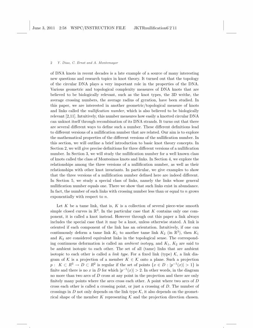
where c ≤ 1 is an additional constant depending on the link type of D. For alter-nating diagrams, we expect an almost equality in (2.3), while for non-alternatingdiagrams (2.3) may still be a large overestimate. Figure 6 shows the case of a mini-mum diagram for the knot 11a263. There are four visible nontrivial flyping circuits(three of which have 3 crossings and one with two crossings) and all crossings inthe circuits are parallel and each crossing belong to one such circuit. It follows thatA = S = 0 and

∑1≤i≤4(|Pi|− 1)+A+S = 7. Thus (2.3) becomes an equality with

the choice of c = 1 since nD = 8. This example shows that it is necessary for us tohave the constant c term in general.

Fig. 6. A minimum diagram knot 11a263 with nD = 8. It has four parallel nontrivial flypingcircuits and each crossing belongs to one of these circuits.

3. Diagram Nullification Numbers of 4-plats and Montesinos Links

In this section we discuss the nullification number nD of 4-plats and Montesinoslinks. The goal is to show that the inequality in (2.3) holds for these links.



A 4-plat is a link with up to two components that admits a minimum alter-nating diagram as shown in Figure 7 where a grey box marked by ci indicates arow of ci horizontal half-twists. Such a link is completely defined by such a vec-tor (c1, c2, . . . , ck) of positive integer entries. Obviously, two vectors of the form(c1, c2, . . . , ck) and (ck, ck−1, . . . , c1) define the same link. However, it is much lessobvious that two such vectors define different 4-plats if they are not reversal ofeach other. For a detailed discussion on the classification of 4-plats see [3,8]. In astandard 4-plat diagram there is an obvious way to assign the notion of parallel oranti-parallel to a single crossing, based on if both strings move in the same right-leftdirection.

c1

c3

ck

ck-1

c2

Fig. 7. A typical 4-plat template. A gray box with label ci represents a horizontal sequence ofci crossings.

A similar schema based on a vector T = (a1, a2, . . . , an) is used to classifyrational tangles. A tangle T is part of a link diagram that consists of a disk thatcontains two properly embedded arcs. For a typical rational tangle diagram seeFigure 8 where the rectangular box contains either horizontal or vertical half-twists.A horizontal (vertical) rectangle labeled ai contains |ai| horizontal (vertical) half-twists and horizontal and vertical rectangles occur in an alternating fashion. Allrational tangles end with an horizontal twists on the right. The ai’s are either allpositive or all negative, with the only exception that an may equal to zero. For aclassification and precise definition of such tangles see [3,8]. We assign the notionof parallel or anti-parallel to a single crossing, based on if both strings move in thesame right-left direction for a horizontal crossing and based on if both strings movein the same up-down direction for a vertical crossing.

Each rational tangle T = (a1, a2, . . . , an) defines a rational number β/α usingthe continued fraction expansion:

β

α= an +

1an−1 + 1

an−1+···+ 1a1

.

Rational tangles are the basic building blocks of a large family of links calledMontesinos links. A Montesinos link admits a diagram that consists of rationaltangles Ti strung together as shown in Figure 9 together with a horizontal number



a1

a2

a3

a4

a5

a6

a1 a2

a3

a4

a5

Fig. 8. A rational tangle diagram T given by the vector T = (a1, a2, . . . , an). On the left is adiagram with n odd (n = 5) and on the left is a diagram with n even (n = 6). A small rectanglewith label ai contains |ai| half-twists, where ai’s are either all positive or all negative, with theonly exception that an may equal to zero.

of |e| half-twists (as indicated by the rectangle in the figure). Such a diagram iscalled a Montesinos diagram. We say that a Montesinos diagram is of type I ifthe orientations between the two arcs connecting any two adjacent tangles in thediagram are parallel. In this case the orientations between the two arcs connectingany two other adjacent tangles in the diagram must be parallel as well. We say thatdiagram is of type II otherwise.

A1A2 As

e

Fig. 9. An illustration of a Montesinos link diagram D = K(T1, T2, . . . , Tt, e) where each Ti is arational tangle.

Let βi

αibe the rational number whose continued fraction expansion is the vector

that defines the rational tangle Ti. We will sometimes write K(T1, T2, . . . , Tt, e)as K( β1

α1, β2

α2, . . . , βt

αt, e). It is known that a Montesinos link admits a Montesinos

diagram satisfying the following additional condition: | βi

αi| < 1 for each i (hence the

continued fraction of βi

αiis of the form (ai,1, ai,2, · · · , ai,ni , 0), where ai,j > 0). See

[3] for an explanation of this and the classification of Montesinos links in general.For a Montesinos link K, let DK be a Montesinos diagram of K that satisfies thiscondition and let Pi be the set of indices i such that ai,j consists of parallel crossingsand Ai be the set of indices i such that ai,j consists of anti-parallel crossings. Wehave the following theorem.

Theorem 3.1. Let K be a Montesinos link with Montesinos diagram DK =



K( β1α1

, β2α2

, . . . , βt

αt, e), where | βi

αi| < 1. Then the number of Seifert circles in DK

is given by the following formula

s(DK) =

{∑ti=1(

∑j∈Ai

(|ai,j | − 1) + |Pi|) + 2 if DK is of type I,∑ti=1(

∑j∈Ai

(|ai,j | − 1) + |Pi|) + |e|+ c if DK is of type II,

where c = 2 if e = 0 and all tangles end with anti-parallel vertical twists, and c = 0otherwise.

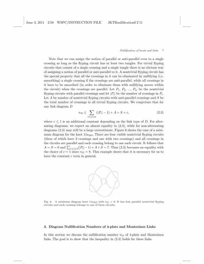
Proof. Consider one of the tangle diagrams βi

αi= (ai,1, ai,2, · · · , ai,ni

, 0). If thecrossings corresponding to ai,j have parallel orientation, then the crossings corre-spond to ai,j−1 and ai,j+1 must have anti-parallel orientation. This can be seen asfollows: Assume that ai,j represents |ai,j | vertical twists with a parallel orientation,see Figure 10. Assume further that both strings are oriented upwards. Then we havetwo strands entering the tangle marked by the dashed oval in Figure 10 from below.Therefore the other two strands of that tangle must have an exiting orientation.This implies that the half-twists at ai,j−1 and ai,j+1 must be anti-parallel. A similarargument holds if ai,j represents horizontal twists with a parallel orientation.

P

A

A

ai,j

ai,j+1

ai,j-1

Fig. 10. The local structure of parallel and anti-parallel orientations and the Seifert circle struc-ture resulting from nullification under the assumption that ai,j is vertical and has parallel orien-tation .

Moreover, there is a Seifert circle that uses the boxes of all three entries ai,j−1,ai,j and ai,j+1 as shown in the Figure 10. This implies that the dashed arcs at thetop left and bottom left of the tangle marked by the dashed oval in Figure 10 mustbelong to the same Seifert circle. It is easy to see that these properties are the sameif ai,j consists of horizontal twists.

Note that after nullification the two arcs in the tangle Ti are changed to a set ofdisjoint Seifert circles and two disjoint arcs connecting two of the four endpoints ofthe tangle. The Seifert circles generated be nullification can be grouped into threedifferent categories. The first group consists of the small Seifert circles, namelythose generated by two consecutive half-twists that are anti-parallel. Clearly, if



|ai,j | > 1 and the corresponding crossings are anti-parallel, then there are |ai,j | − 1such small circles. The second group consists of the medium sized Seifert circles,namely the Seifert circles that are not small but are contained within one of tanglesTi. The two Seifert circles shown in Figure 10 are medium sized ones since they arecontained in a tangle and involve parallel crossings. The third group consists of therest of the Seifert circles. These are Seifert circles that involve more than one tangleand are called large Seifert circles. Figure 10 also shows that for each ai,j that isparallel, one of the two arcs after nullification belongs to a medium Seifert circleand the other belongs to a large Seifert circle. The only exception occurs when ai,j

consists of parallel half twists and is the last nonzero entry of the tangle, that isj = ni. In this case both arcs belong to large Seifert circles.

We have thus shown the following:

(i) There are∑t

i=1

∑j∈Aj

(|ai,j | − 1) small Seifert circles.

(ii) There are −p+∑t

i=1 |Pi|medium Seifert circles where p is the number of tanglesTi where ai,ni consists of parallel half twists.

If DK is of type I, then each ai,ni consists of anti-parallel twists and p = 0.Furthermore, e consists of parallel twists as well and it is easy to see that there areexactly two large Seifert circles. (One passes through all the tangles at the bottomand the other weaves through all tangles in a more complex path). This proves thefirst case of the theorem.

Now assume that DK is of type II. If a tangle Ti ends with parallel (anti-parallel)vertical twists then after nullification the arc with one end at the NW corner willconnect to the SW corner (NE) corner. If we assume that e = 0 then we can seethat after nullification there will be exactly p of the large Seifert circles when p isnonzero and exactly 2 if p = 0. If e 6= 0 then there will be an additional |e| − 1small circles and the number of large Seifert circles changes by minus one if p = 0and increases by plus one if p 6= 0. This proves the second case of the theorem.

Corollary 3.2. Let K be the Montesinos link represented by the diagram DK =K( β1

α1, β2

α2, . . . , βt

αt, e), where | βi

αi| < 1 and e is an integer. Then we have

nd(K) ≤{∑t

i=1(∑

j∈Pi(|ai,j | − 1) + |Ai|) + |e| − 1 if DKis of type I,∑t

i=1(∑

j∈Pi(|ai,j | − 1) + |Ai|)− c + 1 if DKis of type II,

where c = 2 if e = 0 and all tangles end with anti-parallel vertical twists, and c = 0otherwise. Moreover if DK is alternating, then we have equality.

Proof. It suffices to prove the statement of equality for an alternating Montesinoslink. In this case the Corollary follows from Theorem 3.1 and the relationshipnD(K) = Cr(D)−s(D)+1 for any alternating reduced diagram D of the alternatingK.



Since a 4-plat is a Montesinos link that contains only one rational tangle, wehave the following. (Note that a 4-plat is also obtained if there are two rationaltangles in the Montesinos link. However this is not important in this context, see[3].)

Corollary 3.3. Let K be the 4-plat defined by the vector (a1, a2, . . . , an), P be theset of indices i such that ai consists of parallel crossings and A be the set of indicesi such that ai consists of anti-parallel crossings. Then

nd(K) =∑

i∈P

(|ai| − 1) + |A|.

Proof. Consider the 4-plat as the Montesinos link given by DK = K( β1α1

, e), whereβ1α1

= (a1, a2, . . . , an−1, 0) and e = an. If an−1 is zero then K is just an (e, 2) toruslink and the statement is true. If an−1 is not zero then we apply Corollary 3.2. IfDK is of type I then e is parallel and in the formula of Corollary 3.2 we count e asparallel and |e| − 1 = |an| − 1 in the formula of the Corollary. If DK is of type IIthen e is anti-parallel and will be counted as the +1 in Formula in Corollary 3.2.

4. The Nullification Numbers and other Link Invariants

In this section we explore further the relationships among the three nullificationnumbers n(K), nr(K) and nd(K), as well as their relationships with some other linkinvariants.

4.1. The case of alternating links.

First let us consider the alternating links. We have the following theorem.

Theorem 4.1. If K is an alternating link then we have nd(K) = nr(K).

Proof. Since we already have nr(K) ≤ nd(K), it suffices to show that nr(K) ≥nd(K). Let cr(K) = n. Assume that nr(K) is obtained by smoothing crossings c1,c2,..., cm first in a reduced alternating diagram D of K. This results in a diagramD1 with n − m crossings that is still alternating. Assume further that nr(K) isobtained by deforming D1 to a minimum diagram D2 and some crossings in it arethen smoothed. D2 is necessarily alternating since D1 is alternating and D2 sharethe same knot type with D1. On the other hand, D1 can be changed to a reducedalternating diagram D′

1 by performing all possible reduction moves as shown inFigure 11. D′

1 is also minimum since it is reduced and is alternating. Thus it isflype equivalent to the diagram D2. Note that for each crossing reduction move as



shown in Figure 11, one crossing is removed and the number of Seifert circles isreduced by one at the same time. Thus m + nD2 = m + Cr(D2)− s(D2) + 1 = m +Cr(D′

1)−s(D′1)+1 = s+Cr(D1)−s(D1)+1 = Cr(D)−s(D)+1 = nd(K). Therefore

no reduction in the number of nullification steps can be gained by moving to thediagram D2. Since D2 is still alternating, moving to other minimum diagrams aftersmoothing some crossings in it will not result in a nullification number reductioneither by the same argument.

A B

Fig. 11. A reducible alternating diagram contains a single crossing that splits the diagram intotwo parts. Rotation of one part (either A or B) in a proper direction by 180◦ will eliminate onecrossing while preserving the alternating property of the diagram.

On the other hand, even for alternating links, the difference between n(K) andnr(K) can be as large as one wants.

Theorem 4.2. For any given positive integer m, there exists an alternating knotK such that nr(K)− n(K) = nd(K)− n(K) > m.

Proof. As shown in Figure 12, the 4-plats of the vector form (−k,−2,−1, 2, k) allhave general nullification number one, where k is any positive integer.

Fig. 12. The 4-plats (−k,−2,−1, 2, k) have nullification number one. Here an example with k = 3is shown. Smoothing the crossing in the center realizes n(K) = 1.

Notice that (−k,−2,−1, 2, k) can be isotoped to (1, k − 1, 3, 1, k) as shown inFigure 13, which is alternating. Thus we have an alternating knot K with generalnullification number one. For the minimum diagram of K given in Figure 13 we have,by Corollary 3.3 or equation 2.1, nr(K) = nd(K) = (2k + 4) − 5 + 1 = 2k. So thedifference between the diagram nullification number and the general nullificationnumber is > m if k > (m + 1)/2.



Fig. 13. The 4-plat of Figure 12 in a minimum diagram with vector form (1, k − 1, 3, 1, k) fork = 3.

4.2. The case of non-alternating links.

In order to show that nr(K) and nd(K) are indeed different in general, we need todemonstrate the existence of knots/links K such that nr(K) < nd(K). Because ofTheorem 4.1, such examples can only be found in non-alternating knots and links.Worse, there are no known methods or easy approaches in finding such examples.This subsection is thus devoted to the construction of one single such example.

First, let us observe that the knot 820 has the following special property. Theleft of Figure 14 shows that nd(820) = nr(820) = nd(820) = 1. However, afterapplying a simply isotopy as shown on the right side of Figure 14, the new diagramcan no longer be nullified by smoothing only one crossing. One has to smooth twocrossings.

Fig. 14. Left: A minimum knot projection M of the knot 820 that can be nullified by smoothingthe crossing circled. Right: A non-minimum diagram N of 820 that requires the smoothing of twocrossings in order to be nullified (two such crossings are marked with circles).

Now we would like to construct an example using this observation. We constructa three component link L by adding two simple closed curves to N as shown inFigure 15 (drawn by thickened lines). The diagram DL of Figure 15 can be shownto be adequate hence is minimum [8]. Assign the orientations to the components asshown in Figure 15.

It is easy to see that nullifying the two adjacent crossings marked in Figure 15allows the new components to be removed by an ambient isotopy. The resultingdiagram is N which can be further isotoped to M . Thus by the definition of nr we



Fig. 15. A 3-component link L with nr(L) ≤ 3 and nd(L) = 4.

have nr(L) ≤ 3.

Lacking a more elegant method, we took a programmatic approach for the con-firmation that nD(L) > 3. First, we observe that the diagram of Figure 15 is theonly minimum diagram of L up to trivial isotopies. This follows from the fact thatif we remove either one of the new components we obtain an alternating and henceminimum diagram that admits no flypes. Thus any diagram of such a two com-ponent link has to look like the one shown. The two additional components are“parallel” and therefore the only change we can make is to exchange them. Thishowever does not change the diagram. We then implemented the nullification pro-cedure which yielded all knot/link diagrams obtained by all possible combinationsof 3 or less crossing smoothing steps on DL. Using a Gauss code modification pro-gram and the Mathematica c©KnotTheory package’s Jones polynomial computationwe were able to verify that none of these resulted in a knot/link with the polynomialof a trivial knot/link. Since nd(L) ≤ 4 by our construction of L, we have shownthat nd(L) = 4. Thus we have shown an example of a three component link L withnr(L) ≤ 3 and nd(L) = 4.

4.3. The genus, unknotting number and the signature vs n(K).

There is a simple inequality between the nullification number and the unknottingnumber:

Lemma 4.3. Let K be any knot then n(K) ≤ 2u(K), where u denotes the unknottingnumber of a knot.

Proof: It suffices to show that a strand passage can be realized by two nullifi-cation moves. This is shown in Figure 16.



Fig. 16. Nullifying two crossings is equivalent to a strandpassage.

The next theorem shows that an inequality as given in Lemma 4.3 does notexist the other way around, that is the unknotting number can not be bound fromabove by a multiple of the general nullification number.

Theorem 4.4. For any given positive integer m, (1) there exists an alternatingknot K such that g(K) − n(K) > m where g(K) is the genus of K and (2) thereexists a link K such that u(K)−n(K) > m. In other words, the general nullificationnumber does not impose a general upper bound on the genus and the unknottingnumber of a link.

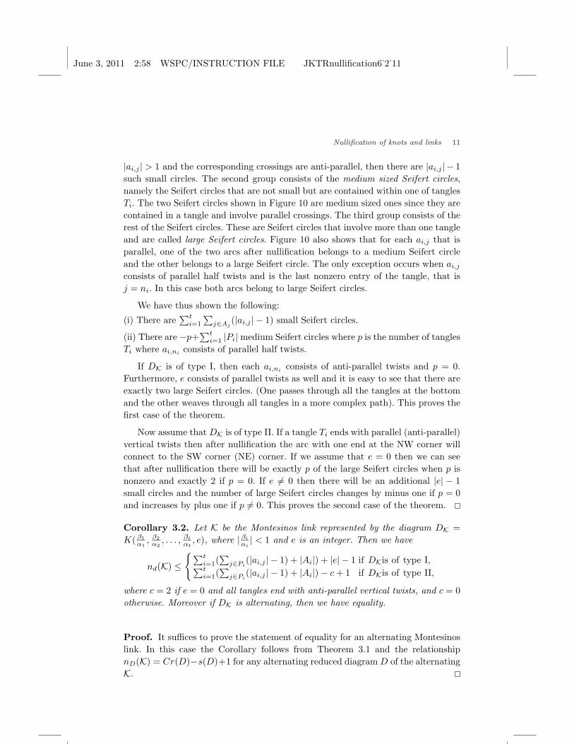
Proof. Notice that the genus of the knot K in Figure 13 is k. Thus if k > m + 1,then g(K)−n(K) = k−1 > m. For the second part of the theorem, consider the toruslink T (3n, 3) (n is an arbitrary positive integer) as shown in Figure 17, in whichtwo of the three components are oriented in parallel (say clockwise) and the thirdcomponent is oriented in the other direction (say counterclockwise). By nullifyingany one of the crossings between two components with opposite orientations inFigure 17 we obtain the unlink. Thus n(T (3n, 3)) = 1. On the other hand, by theBennequin Conjecture [1,27], the unknotting number of T (3n, 3) is 3n and the resultof the second part of the theorem follows.

The signature σ(K) of a link K is defined as the signature of the matrix M +MT where M is the Seifert matrix obtained from any regular diagram of K. Thedefinition and computation of a Seifert matrix is beyond the scope of this paperand we refer the reader to any standard text in knot theory such as [3,8].

Theorem 4.5. For any oriented link K we have n(K) ≥ |σ(K)|.

Proof. We use an approach similar to the one used in the proof of Theorem 6.8.2in [8] (where the relationship between the signature and the unknotting number isinvestigated). We will need the following lemma 4.6 from [14]. A σ-series of an n×n

matrix of rank r is a sequence of submatrices ∆i such that (i) ∆i is an i× i matrix;(ii) ∆i is obtained from ∆i+1 by removing a single row and a single column; and(iii) no two consecutive matrices ∆i and ∆i+1 are singular when i < r.



Fig. 17. The torus link T (3n, 3) with one component of reverse orientation has nullificationnumber one and unbounded unknotting number. The special case n = 3 is shown here.

Lemma 4.6. [14] Let A be a symmetric n× n matrix with a σ-series as describedabove. Put ∆i = 1. Then the signature of A is given by

σ(A) =n∑

i=1

sgn(det(δi−1) det(δi)),

where sgn() is the sign function.

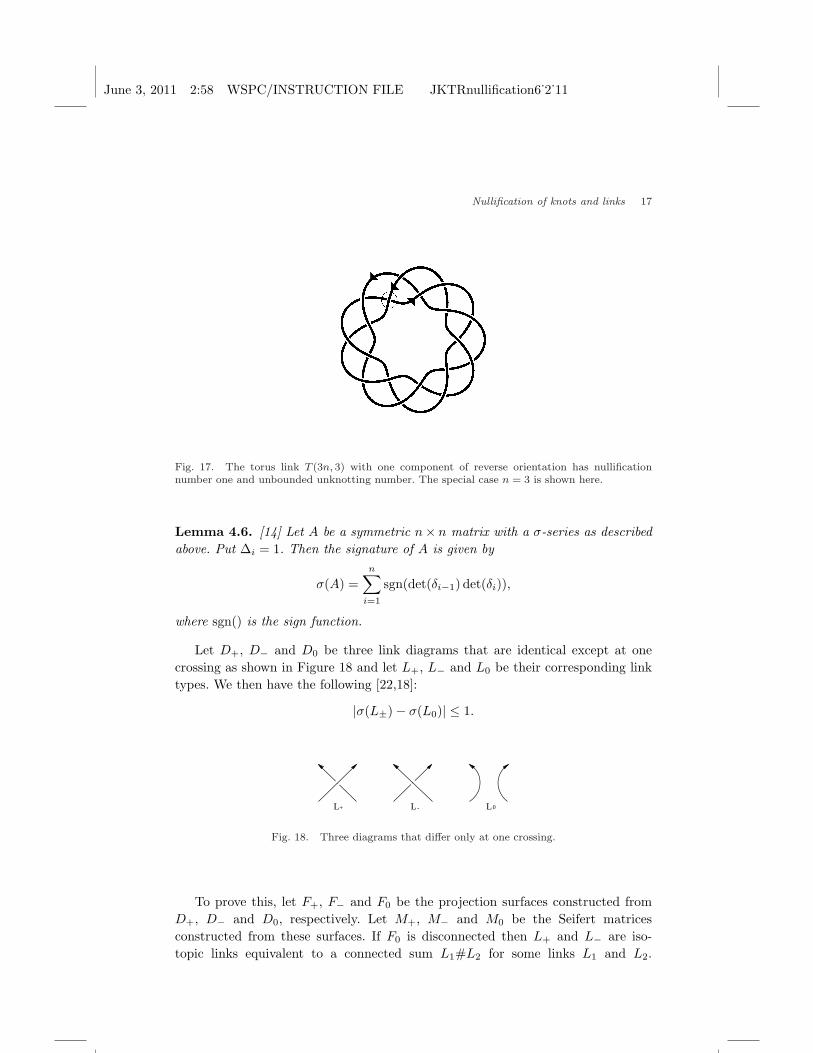
Let D+, D− and D0 be three link diagrams that are identical except at onecrossing as shown in Figure 18 and let L+, L− and L0 be their corresponding linktypes. We then have the following [22,18]:

|σ(L±)− σ(L0)| ≤ 1.

L L L+ - 0

Fig. 18. Three diagrams that differ only at one crossing.

To prove this, let F+, F− and F0 be the projection surfaces constructed fromD+, D− and D0, respectively. Let M+, M− and M0 be the Seifert matricesconstructed from these surfaces. If F0 is disconnected then L+ and L− are iso-topic links equivalent to a connected sum L1#L2 for some links L1 and L2.



Therefore in this case σ(L1#L2) = σ(L1) + σ(L2) = σ(L1 t L2) = σ(L0) andσ(L+)− σ(L0) = σ(L−)− σ(L0) = 0.

If F0 is connected then F+ and F− are obtained from F0 by adding a twistedrectangle at the crossing that is switched or eliminated. Therefore the Seifert ma-trices M+ and M− have one additional column and row added to the Seifert matrixM0 as shown below for M+ where b is an additional loop that passed through theadded rectangle and back through the rest of the surface F0 and (a1, · · · , an) is abasis for H1(F0).

a+1 · · · a+

n b+

a1 v1

... M0

...an v1

b λ+1 · · · λ+

n β

We write A∗ = M∗ + MT∗ where ∗ = +,− or 0. The matrices A∗ may not be

singular, however they are non-singular if the corresponding L∗ is a knot. In eithercase we can use Lemma 4.6 to obtain that:

σ(A±)− σ(A0) = sign(det(A±) det(A0)) = δ,

where ∗ = + or − and from this it follows that δ = ±1 or 0.

This result implies that in any nullification sequence of K, the smoothing of acrossing can only change the signature by at most one. Since the signature of thetrivial link is zero and n(K) is the minimum number of smoothing moves neededto change K to a trivial link, it follows that |σ(K)| ≤ n(K).

Corollary 4.7. Let K be any knot then |σ(K)| ≤ n(K) ≤ 2u(K). In particular if|σ(K)| = 2u(K), then |σ(K)| = n(K) = 2u(K).

Note that the above Corollary is quite powerful if one wants to determine theactual general nullification number for small knots in the knot table. In [10] thegeneral nullification number of all but two knots of up to 9 crossings is determined.The following corollary is an immediate consequence of Theorem 4.5 and the factthat all knots have even signatures [21].

Corollary 4.8. If K is a knot and n(K) = 1, then σ(K) = 0.

In [13] the signature of an oriented alternating link K is related to the writhevia the concept of nullification writhe. Let D be a reduced alternating diagram ofK and in this diagram we have a nullification sequence of crossings c1, c2, ... , ck,where k = nD = nd(K), then the nullification writhe introduced in [6] is defined as



the sum of the signs of the crossings c1, c2, ... , ck and is denoted by Wr(nD). Wehave:

Theorem 4.9. [13] For an alternating oriented link σ(K) + Wr(nD) = 0.

The example of the 4-plat given in Figures 12 and 13 (with k = 3) representsthe knot 1022. This knot has σ(1022) = 0 (In fact we can see that a nullificationsequence for the diagram in Figure 13 has a nullification sequence of three positiveand three negative crossings.) On the other hand we see that the inequality inTheorem 4.5 is strict since n(1022) = 1. Note that the signature of a 4-plat can becomputed by the following explicit formula.

Theorem 4.10. [25] Let K be a 4-plat knot then

σ(K) =2g∑

i=1

(−1)i−1sign(ai),

where the vector (a1, a2, ..., a2g) is a continued fraction expansion of K using onlyeven integers. (Such a continued fraction expansion is called an even continuedfraction expansion.)

In fact, the length of the even continued fraction expansion is 2g where g is thegenus of K [8]. We also have the following two corollaries:

Corollary 4.11. If D is a reduced alternating diagram of an alternating orientedlink K such that all crossings in a nullification sequence of D have the same sign,i.e., |Wr(nD)| = nD, then nd(K) = n(K).

Proof. We have |σ(K)| = |Wr(nD)| = nD = nd(K) ≥ n(K) ≥ |σ(K)|. Thus theequality holds.

Corollary 4.12. For any even positive integer k the number of knots K with Cr(K)crossings and |n(K)| ≥ k grows exponentially with

√Cr(K).

Proof. Let us assume for simplicity that m = Cr(K) is odd and consider the 4-plats K with a vector form (a1, a2, ..., a2g) such that ai is even and aiai+1 < 0 forall i. Then σ(K) = 2g. The crossing number Cr(K) is given by [8]

Cr(K) = (2g∑

i=1

|ai|)− 2g + 1.

If m = Cr(K) is sufficiently large then we can generate such a vector by partitioningthe positive integer m + 2g − 1 into 2g even integers bi where bi ≥ 2. Here we set



ai = (−1)i+1 · bi. This is equivalent to partitioning the integer m − 2g − 1 into 2g

even integers ci where ci ≥ 0 which in turn is equivalent to the number of partitionsof the integer (m− 1)/2− g into 2g integers di where di ≥ 0. A standard result innumber theory about the number of partitions then implies the result.

5. Nullification Number One Links

In this section we explore the special family of links whose general nullificationnumber is one. The first question is about the number of such links. In the followingwe will give a partial answer to this question. Let (a1, a2, . . . , ak) be the standardvector form of a rational link K corresponding to the rational number p

q . Considerthe rational link K′ defined by the vector (a1, a2, . . . , ak, ε,−ak, . . . ,−a1), whereε = ±1. Let a

b be the fraction for K′, then we can get ab = p2

(ε+pq) by using amethod from [23]. Furthermore, when K is a knot, K′ is also a knot and has generalnullification number 1.

Two fractions p2

(ε1+pq) and p2

(ε2+pq′) represent the same knot iff ε1 + pq ≡ ε2 +pq′

(mod p2

)or (ε1 + pq) (ε2 + pq′) ≡ 1

(mod p2

). If ε1 = ε2 then this yields pq ≡

pq′(mod p2

)or pq ≡ −pq′

(mod p2

). So q ≡ q′ (mod p) or q ≡ −q′ (mod p). This

implies that different fractions pq result in different 4-plats p2

(ε1+pq) (up to mirrorimages).

Thus we have shown that for each rational knot K, there exists a rational knot K′(unique up to mirror image) with nullification number one. Furthermore, Cr(K′) =2

∑ki=1 ai = 2Cr(K). Since the number of rational knots grows exponentially, we

have shown the following theorem.

Theorem 5.1. The number of knots K with n(K) = 1 and Cr(K) ≤ n growsexponentially in terms of n.

We would like to point out that the rational knots considered above do notcontain all nullification number one rational knots. We give two additional exampleof 4-plat knot families with nullification number one. In the two examples we donot follow the usual vector notation for rational knots such as in [3]. Instead weadopt the sign assignment convention as shown in Figure 19 for the crossings thatare in the boxes in Figures 20 and 21. Here the crossings have two ends marked ason the bottom and the other two ends as on the top and therefore the crossings inFigure 19 can not be rotated by 90 degrees.

Example 5.2. Consider the rational knot defined by a vector of the form(−2a,−2,−2b, 2, 2a, 2b), where the first 2a means a sequence of 2a positive cross-ings between the first and second strings using the sign convention given in Figure



_

(b)(a)

+

Fig. 19. Crossing (a) is positive and crossing (b) is negative. Notice that this is not how the signof a crossing in a rational knot is assigned and is only used for the examples here.

19, and so on, as shown in the first diagram of Figure 20. Note that the actualsign convention of the crossings in the boxes does not matter, as long as boxes withopposite signs have twists that are mirror images of each other. By a rotation in-volving the two top boxes in the first diagram, followed by a proper flype involvingthe resulting two boxes and some other isotopes, one can see that the first diagramis equivalent to the second one. From there it is relatively easy to see the seconddiagram can be isotoped to the third diagram. If we smooth the crossing as markedin the third diagram, we end up with the fourth diagram. It is not too hard to seethat the fourth diagram is the trivial knot. Thus this family of rational knots is alsoof general nullification number one. The details of the isotopies used are left to thereader as an exercise.

−2a

−2b

2b −2b2b2b 2b −2b

−2b

2a−

2a

2a−

2a

2a

−2a

2a

Fig. 20. The family of rational knots with the vector form (−2a,−2,−2b, 2, 2a, 2b) using the signconvention as defined in Figure 19. These knots have general nullification number one, where thesigned number on a box indicates the number of half twists with the shown sign.

Example 5.3. The second example (of other nullification number one rationalknots) is similarly constructed. Here the knot family consists of rational knots de-fined by vectors of the form (−2b,−2,−2a, 2b, 2, 2a) as shown in the first diagramof Figure 21. The isotopes leading to the single nullification crossing of the knot are



illustrated in the rest of the figure.

2a

2b−

2a−

2b2a

2a −2a

−2b 2b

2a −2a

−2b 2b

−2b

−2a

2b

Fig. 21. Another family of rational knots (defined by vectors of form (−2b,−2,−2a, 2b, 2, 2a)using the sign convention as defined in Figure 19) with general nullification number one.

Note that the actual sign convention as shown in in Figure 19 does not matteras long as the the crossings in the two boxes with the same label have oppositehandedness. These three families of rational knots have one interesting property incommon, namely that they are all ribbon knots (to be defined next). In fact it wasconjectured in [5] that these were the only rational ribbon knots. This conjecturewas recently proven in [17].

Let K be a link in S3, and b : I × I → S3 be an imbedding such that b (I × I)∩K = b (I × ∂I). Let Kb = {K \ b(I × ∂I)} ∪ b (∂I × I). If Kb is a link with anorientation compatible with K then Kb is called a banding of K, or is obtainedfrom K by band surgery (along b). It turns out that nullification and banding areequivalent operations. See Figure 22.

Fig. 22. Top: Nullification via banding. Bottom: Banding via nullification.



A knot K is a ribbon knot if it is a knot obtained from a trivial (m+1)-componentlink by band surgery along m bands for some m. The minimum of such number m

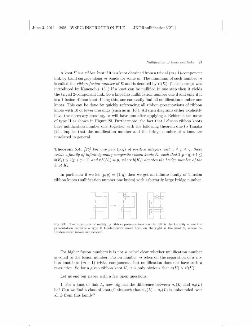
is called the ribbon-fusion number of K and is denoted by rf(K). (This concept wasintroduced by Kanenobu [15].) If a knot can be nullified in one step then it yieldsthe trivial 2-component link. So a knot has nullification number one if and only if itis a 1-fusion ribbon knot. Using this, one can easily find all nullification number oneknots. This can be done by quickly referencing all ribbon presentations of ribbonknots with 10 or fewer crossings (such as in [16]). All such diagrams either explicitlyhave the necessary crossing, or will have one after applying a Reidemeister moveof type II as shown in Figure 23. Furthermore, the fact that 1-fusion ribbon knotshave nullification number one, together with the following theorem due to Tanaka[26], implies that the nullification number and the bridge number of a knot areunrelated in general.

Theorem 5.4. [26] For any pair (p, q) of positive integers with 1 ≤ p ≤ q, thereexists a family of infinitely many composite ribbon knots Ki such that 2(p+q)+1 ≤b(Ki) ≤ 2(p+ q +1) and rf(Ki) = p, where b(Ki) denotes the bridge number of theknot Ki.

In particular if we let (p, q) = (1, q) then we get an infinite family of 1-fusionribbon knots (nullification number one knots) with arbitrarily large bridge number.

Fig. 23. Two examples of nullifying ribbon presentations: on the left is the knot 61 where thepresentation requires a type II Reidemeister move first, on the right is the knot 89 where noReidemeister moves are needed.

For higher fusion numbers it is not a priori clear whether nullification numberis equal to the fusion number. Fusion number m relies on the separation of a rib-bon knot into (m + 1) trivial components, but nullification does not have such arestriction. So for a given ribbon knot K, it is only obvious that n(K) ≤ rf(K).

Let us end our paper with a few open questions.

1. For a knot or link L, how big can the difference between nr(L) and nd(L)be? Can we find a class of knots/links such that nd(L)− nr(L) is unbounded overall L from this family?



2. If D′ is a diagram obtained from an alternating (reduced) diagram D byone crossing change (so D′ is no longer alternating and it may even be the trivialknot/link), how much smaller is nD′ compared to nD? For alternating knots withunknotting number one, nD′ is simply zero hence this difference can be as largeas one wants. However, is there a way to relate this problem with the unknottingnumbers in general?

3. By nullifying one crossing in a diagram D (not necessarily minimum) of aknot/link K, we obtain a new knot/link. How many different knots/links can beobtained this way? In particular, is this number bounded above by Cr(K)?

Acknowledgments

Y. Diao is currently supported by NSF Grants #DMS-0920880 and #DMS-1016460,C. Ernst was partially supported by an internal summer grant from WKU in 2010and is currently supported NSF grant #DMS-1016420.

References

[1] D. Bennequin, L’instanton gordien (d’apres P.B. Kronheimer et T.S. Mrowka), As-terisque 216 (1993), pp. 233-277.

[2] D. Buck and C. V. Marcotte, Classification of tangle solutions for integrases, a proteinfamily that changes DNA topology, J. Knot Theory Ramifications 16(8) (2007), pp.969-995.

[3] G. Burde and H. Zieschang, Knots, de Gruyter, Berlin, 1986.[4] J. Calvo, Knot enumeration through flypes and twisted splices, J. Knot Theory Rami-

fications 6 (1997), pp. 785–798.[5] A. J. Casson and C. McA. Gordon, Cobordism of classical knots, In ‘A la recherche

de la topologie perdue, volume 62 of Progr. Math., pp. 181-199. Birkhauser, Boston,1986.

[6] C. Cerf, Nullification writhe and chirality of links, J. Knot Theory Ramifications 6(1997), pp. 621–632.

[7] C. Cerf and A. Stasiak, A topological invariant to predict the three-dimensional writheof ideal configurations of knots and links, PNAS 97(8) (2000), pp. 3795–3798.

[8] P. Cromwell, Knots and Links, Cambridge University Press, 2004.[9] Y. Diao, C. Ernst and A. Stasiak, A Partial Ordering of Knots Through Diagrammatic

Unknotting, Journal of Knot Theory and its Ramifications 18(4) (2009), 505–522.[10] C. Ernst, A. Montemayor and Andrzej Stasiak, Nullification of Small knots, preprint

(2010).[11] I. Grainge, M. Bregu, M. Vazquez, V. Sivanathan, S. C. Ip and D. J. Sherratt, Un-

linking chromosome catenanes in vivo by site-specific recombination, EMBO Journal26 (2007), pp. 4228-4238.

[12] J. Hoste and M. Thistlethwaite, Knotscape, www.math.utk.edu/∼morwen/knotscape.[13] C. V. Q. Hongler, On the nullification writhe, the signature and the chirality of al-

ternating links, Journal of Knot Theory and its Ramifications 10(4) (2001), 537–545.[14] B. W. Jones, The arithmetic theory of quadratic forms, Carus Math. Monographs,

1950.



[15] T. Kanenobu, Band surgery on knots and links, OCAMI Preprint Series, 2009.http://math01.sci.osaka-cu.ac.jp/OCAMI/preprint/2009/09 08.pdf.

[16] A. Kawauchi, A Survey of Knot Theory, Birkhauser, Basel, 1996.[17] P. Lisca, Lens spaces, rational balls and the ribbon conjecture, Geom. Topol. 11

(2007), pp. 429-472.[18] C. Manolescu and P. Ozsvath, On the Khovanov and knot Floer homologies of quasi-

alternating links, Proceedings of Gokova Geometry/Topology Conference (GGT)2007, Gokova (2008), pp. 60–81.

[19] W. Menasco and M. Thistlethwaite, The Tait flyping conjecture, Bull. Amer. Math.Soc., 25 (1991), pp. 403–412.

[20] W. Menasco and M. Thistlethwaite, The classification of alternating links, Ann.Math., 138 (1993), pp. 113–171.

[21] K. Murasugi, Knot Theory and Its Applications, Birkhauser, Boston 1996.[22] K. Murasugi, On a certain numerical invariant of link types, Trans. Amer. Soc. 117

(1965), pp. 387–422.[23] L. Siebenman, Exercices Sur Les Noeuds Rationnels, preprint, Orsay, 1975.[24] D. Sola, Nullification number and flyping conjecture, Rend. Sem. Mat. Univ. Padova,

86 (1991), pp. 1–16.[25] A. Stoimenow, Generating functions, Fibonacci numbers and rational knots, Journal

of Algebra 310(2) (2007), pp. 491–525.[26] T. Tanaka, On bridge numbers of composite ribbon knots, Journal of Knot Theory

and Its Ramifications, 9(3)(2000), pp.423-430.[27] E. W. Weisstein, CRC Concise Encyclopedia of Mathematics, Chapman and Hill

(2002).

nullification of knots and links · june 3, 2011 2:58 wspc/instruction file...

Documents