Mohd Nor Azmi Bin Ab. Patar

TSE

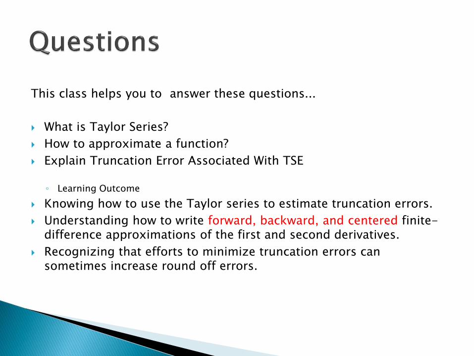
This class helps you to answer these questions...

What is Taylor Series?

How to approximate a function?

Explain Truncation Error Associated With TSE

◦ Learning Outcome

Knowing how to use the Taylor series to estimate truncation errors.

Understanding how to write forward, backward, and centered finite-difference approximations of the first and second derivatives.

Recognizing that efforts to minimize truncation errors can sometimes increase round off errors.

http://numericalmethods.eng.usf.edu 3

Some examples of Taylor series which you must have seen

!6!4!2

1)cos(642 xxx

x

!7!5!3

)sin(753 xxx

xx

!3!2

132 xx

xe x

http://numericalmethods.eng.usf.edu 4

The general form of the Taylor series is given by

32

!3!2h

xfh

xfhxfxfhxf

provided that all derivatives of f(x) are continuous and exist in the interval [x,x+h]

What does this mean in plain English?

As Archimedes would have said, “Give me the value of the function at a single point, and the value of all (first, second, and so on) its derivatives at that single point, and I can give you the value of the function at any other point” (fine print

excluded)

http://numericalmethods.eng.usf.edu 5

Find the value of 6f given that ,1254 f ,744 f

,304 f 64 f and all other higher order derivatives

of xf at 4x are zero.

Solution:

!3!2

32 hxf

hxfhxfxfhxf

4x

246 h

http://numericalmethods.eng.usf.edu 6

Solution: (cont.)

Since the higher order derivatives are zero,

!3

24

!2

2424424

32

fffff

!3

26

!2

2302741256

32

f

860148125

341

Note that to find 6f exactly, we only need the value

of the function and all its derivatives at some other point, in this case

4x

Non-elementary functions such as trigonometric, exponential,

and others are expressed in an approximate fashion using Taylor

series when their values, derivatives, and integrals are computed.

Any smooth function can be approximated as a polynomial.

Taylor series provides a means to predict the value of a function

at one point in terms of the function value and its derivatives at

another point.

Cos(x)

Sin(x)

Example:

To get the cos(x) for small x:

If x=0.5

cos(0.5) =1-0.125+0.0026041-0.0000127+ …

=0.877582

From the supporting theory, for this series, the error is no greater

than the first omitted term.

!6!4!2

1cos642 xxx

x

0000001.05.0!8

8

xforx

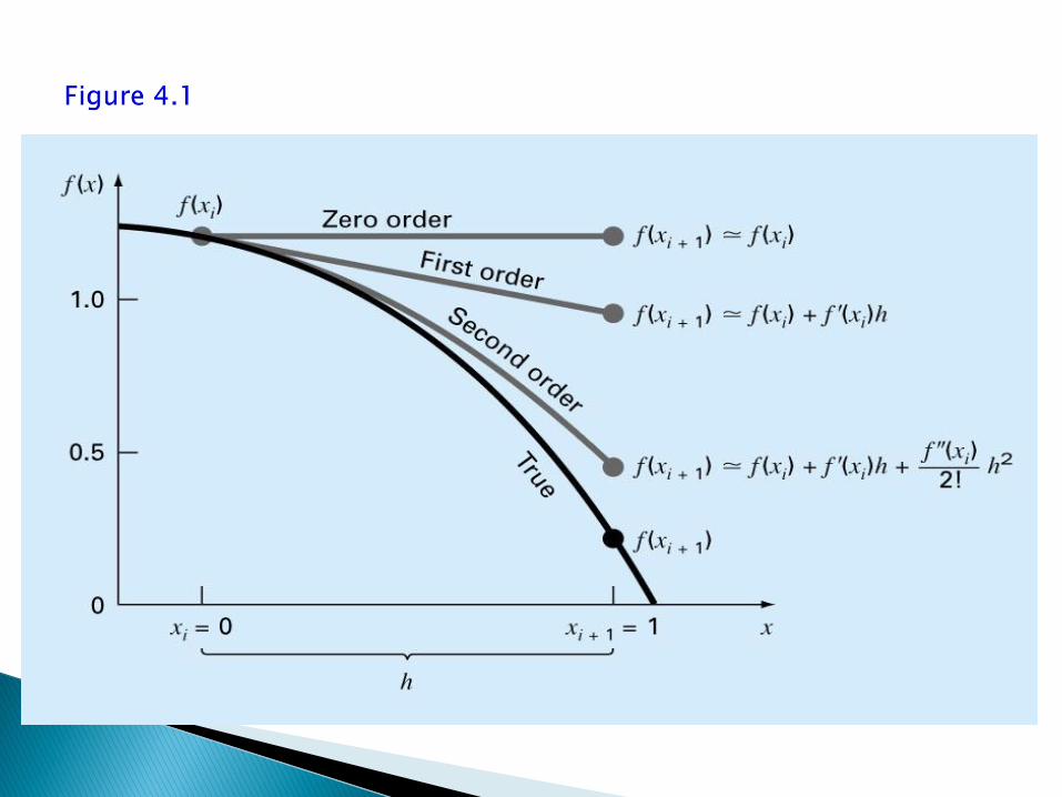
Any smooth function can be approximated as a polynomial.

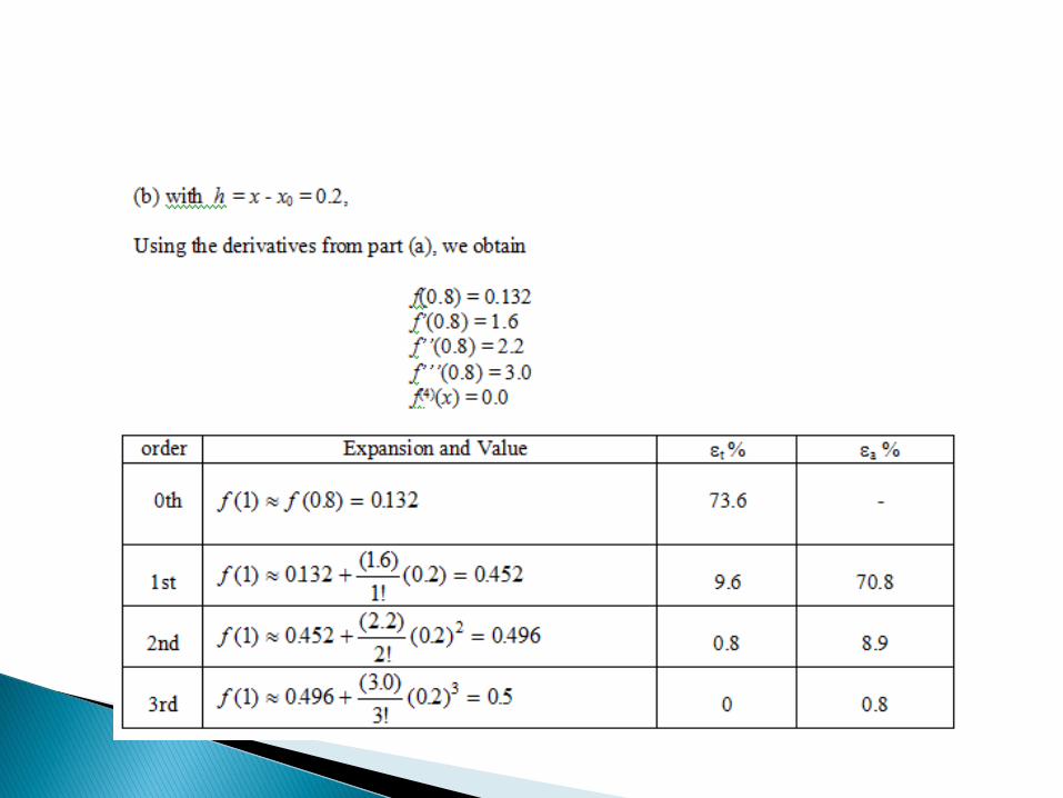
f(xi+1) ≈ f(xi) zero order approximation, only true if xi+1 and xi are very close to each other.

f(xi+1) ≈ f(xi) + f′(xi) (xi+1-xi) first order approximation, in form of a straight line

n

n

ii

n

iiiiiii

Rxxn

f

xxf

xxxfxfxf

)(!

)(!2

))(()()(

1

)(

2

111

(xi+1-xi)= h step size (define first)

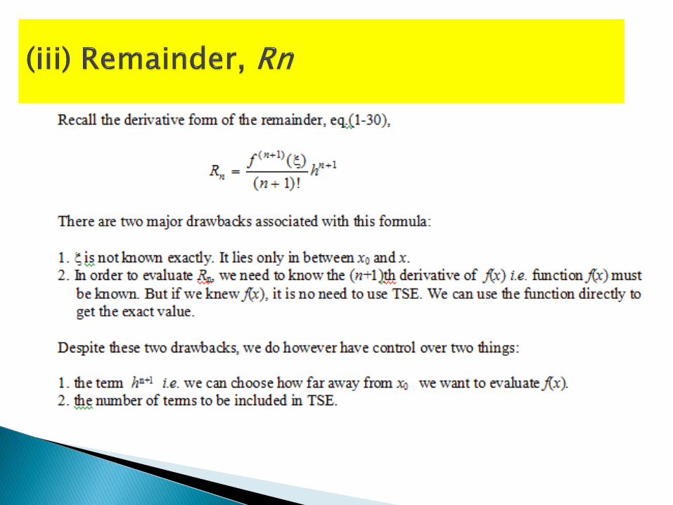
)1()1(

)!1(

)(

n

n

n hn

fR

• Reminder term, Rn, accounts for all terms

from (n+1) to infinity.

nth order approximation

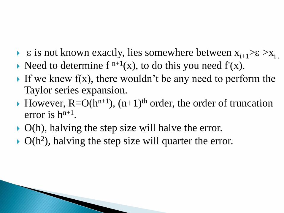
is not known exactly, lies somewhere between xi+1> >xi .

Need to determine f n+1(x), to do this you need f'(x).

If we knew f(x), there wouldn’t be any need to perform the Taylor series expansion.

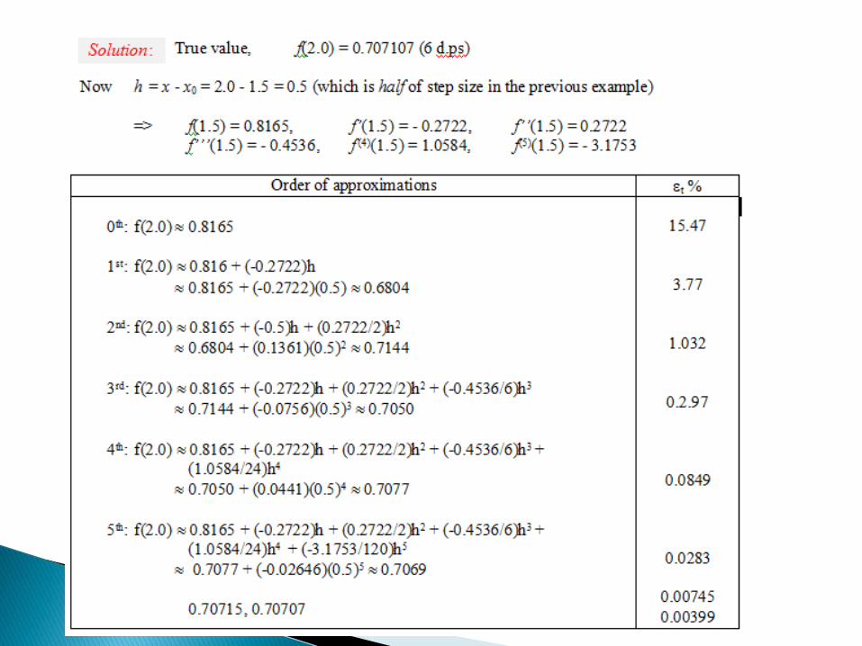
However, R=O(hn+1), (n+1)th order, the order of truncation error is hn+1.

O(h), halving the step size will halve the error.

O(h2), halving the step size will quarter the error.

Truncation error is decreased by addition of terms to the Taylor

series.

If h is sufficiently small, only a few terms may be required to

obtain an approximation close enough to the actual value for

practical purposes.

Example:

Calculate series, correct to the 3 digits.

4

1

3

1

2

11

(i) Taylor Series Expansion (TSE)

Note: Polynomial is an expression of finite length constructed from variables (also known as indeterminates) and

constants, using only the operations of addition, subtraction, multiplication, and non-negative, whole-number exponents.

For example, x2 − 4x + 7 is a polynomial, but x2 − 4/x + 7x3/2 is not, because its second term involves division by the

variable x and because its third term contains an exponent that is not a whole number.

Source: Wikipedia

Note: In mathematics, especially in order theory, an upper bound of a subset S of some partially ordered set (P, ≤) is an element of P

which is greater than or equal to every element of S. Example: 2 and 5 are both lower bounds for the set { 5, 10, 34, 13934 }, but 8 is not.

42 is both upper and lower bound for the set { 42 }; all other numbers are either an upper bound or a lower bound for that set.

Note:

Taylor series provides a means to predict a

function value at one point in terms of the function

values and its derivatives at another point.

A useful way to gain insight into the Taylor series is to build it term by term.

For example, The first term of

the series

For example called the zero-order approximations, indicates that the value of ƒ at the new point is the same as its value at the old point.

This term provides a perfect estimate if the function being approximated is, constant.

However, if the function changes at all over the interval, additional terms of the Taylor series are required to provide a better estimate.

Truncations Errors: error that result from using an approximation in place

of an exact mathematical procedures.

The Mean Value Theorem states that if f(x) is continuous

on [a,b] and differentiable on (a,b) then there exists a

number c between a and b such that

The following applet can be used to approximate the

values of c that satisfy the

conclusion of the Mean Value Theorem.

Simply enter the function f(x) and the values a, b and c.

errorTruncation

ionapproximatorder

ii

st

ii

iii

xx

R

xx

xfxfxf

1

1

1

1

1

)()()('

It is termed a “forward” difference because it utilizes data and to estimate the derivatives.i 1i

A simple steel beam with one end fixed and the other end free has a 30ft length. The beam carries a uniform load of 50 lb/ft, including its own weight. Given that the modulus of elasticity, E and the moment of inertia, I are 1.5 x 108 lb/ft2 and 0.06 ft4, respectively. While associated errors, ∆ of the variables involved are 2 lb/ft, 0.1 ft, 0.01 x 108 lb/ft2 and 0.0006 ft4. Estimate the resulting error in the maximum defection, y. (Hint: Refer to Appendix A)

Appendix A